Science and teaching: Two-dimensional signalling inthe academic job market

Preliminary version. Please do not cite without permission.

Andrea Schneider∗

Helmut Schmidt University, 22043 Hamburg, Germany

AbstractPost-docs signal their ability to do science and teaching to get a tenuregiving universities the possibility to separate highly talented agents from thelow talented. This paper shows that, if time constraints are binding, underweak conditions separating equilibria do not exist impliying that universitiescan partially separate some but not all types. Signalling efforts in thesepartial separating equilibria are higher than in a case where post-docs signaltheir science or teaching ability questioning the efficiency of the current two-dimensional academic appointment system.

Keywords: Multi-dimensional signalling; Academic job market; Teaching and Re-search

JEL classification: I23; D82; J41

1 Introduction

Not later than the 19th century the Germans know the concept of the unity ofresearch and teaching. This idea of Wilhelm von Humboldt has mainly influencedespecially the German higher education system and is still present today. On theother hand post-docs and professors often rail against the double burden of sucha system. These conflicting argumentations in mind economists study the optimaldesign of the university system (e.g. Del Rey 2001, De Fraja and Valbonesi 2008or Gautier and Wauthy 2007) as well as their optimal labour contract behaviour

∗Corresponding author. Tel.: +49-40-6541-3725; Fax +49-40-6541-3409; E-mail:andrea.schneider@hsu-hh.de.

1

(Walckiers 2008). In line with the second part of literature the present paper anal-yses the possibility of separating highly productive agents from the low-productiveones in a model where post-docs can signal their ability to do science and teachingto get a tenure.Argumenting in line with a job market sinalling model it is necessary to mentionthe work of Michael Spence. Spence as the father of signalling models shows educa-tion can be an efficient signal to correct asymmetric information in the job market.It’s due to him that we know about the existence of signalling equilibria (Spence1973; Spence 1974).1 In contrast to Spence who mainly deals with the existenceof equilibria Cho and Kreps (1987) rank equilibria. They implement an intuitvecriterion to eliminate equilibria that are built on unplausible out-of-equilibriumbeliefs. This stronger equilibrium concept is finally the basic equilibrium conceptof the present paper.Up to here all concepts work in a one-dimensional world. Thus, agents send aone-dimensional signal. Since future professors produce a two-dimensional outputconsisting of science and teaching a multi-dimensional set up is needed. Unfor-tunately, papers on multi-dimensional signalling are rare. One of the first is byRochet and Quinzii (1985). This paper analyses in a formal way the differencebetween the one- and multi-dimensional signalling set up. Assuming a separa-ble cost structure they give necessary conditions for the existence of a separatingequilbrium. In the same kind of model Engers (1987) focuses on pareto-dominantseparating equilibria. Armstrong and Rochet (1999) simplify conditions that arenecessary to ensure a separating equilibrium by assuming a discrete type distri-bution. This is also an assumption of the present model. A current paper byKim (2007) is of interest as well because it analyses time binding constraints in atwo-dimensional job market signalling model.The aim of this paper is to analyse separating equilibria in a two-dimensional sig-nalling model that describes the academic job market. Post-docs that differ intheir ability to do research and teaching can signal both talents to get a tenure.As one result separating equilibria of the two-dimensional case can vanish withtime binding constraints. This always happens if teaching (science) productivityof the highly talented is higher than the science (teaching) productivity of thelow-talented. Nevertheless, implying the concept of partial separating equilibria itcan be shown that under weak conditions there is at least one partial separatingequilibrium. More precisely, agents that are highly productive in both outputssend the same signal like the type that is high-talented with respect to the outputthat is more prefered by the universities. What is mportant for policiy implicationsis that the signalling effort in the partial separating equilibrium - although it is

1While Spence’s first paper focuses on the general existence of signalling equilibria thesecond paper highlights the different market forms.

2

smaller than in the two-dimensional separating equilibrium - is higher than in theone-dimensional separating equilibrium. This is of interest if signalling only has aneffect on costs but not on productivity as it is the case in Spence (1973) and alsoin the present model. Thus, if time constraints are binding in the academic jobmarket it could be more efficient to let post-docs only signal on the output thatis more prefered by the universities. Under time binding constraints universitiescan only distinguish highly productive from low-productive types in one dimensionjust like in the one-dimensional case. Having this in mind there is no argument forthe two-dimensional signalling process that is currently observed in reality. It justimplies additional signalling effort. Only weak conditions concerning the rankingof the productivity parameters are necessary to make a separating equilibrium un-der time binding constraints impossible in the two-dimensional case. Thus, agentsthat are highly-talented in both outputs can not be identified by universities.The remaining paper is structured as follows: Section 2 sets the basic model. Theexistence of equilibria is analysed in section 3. While section 3.1 focuses on theone-dimensional case that goes in line with Spence (1973) section 3.2 extends theanalysis to the two-dimensional case. In this part the paper distinguishes betweena situation where time constraints are not binding resulting in the unique sepa-rating equilibrium is most efficient for the universities and a situation where timeconstraints are binding which may lead to the vanishing of the separating equilib-rium. In the second case the existence of partial separating equilibria where sometypes of agents can be separated while others play the same stratgey is analysed.Section 4 concludes.

2 The model

Assume a competitive academic job market with a unit mass of academics. Eachuniversity graduate produces science and teaching which requires specific unob-servable abilities.2 Scientists as well as other labourers are not identical but varyin their abilities. There are four types ij ∈ {HH,HL,LH,LL} of future profes-sors.3 While i denotes research productivity j describes the teaching productivity.Both productivities can be high (H) or low (L). Future professors can signal bothabilities: Science sij and teaching tij , i, j ∈ {L,H}. As in Spence (1973) signalsdo not have any influence on productivity. Agents use the signals to influence theuniversities’ beliefs on their abilities. Thus, the pre-tenure research and teach-ing outputs serve as a signal for post-tenure productivities. However, there is atime binding constraint sij + tij = l. Signalling effort can not be higher than the

2In the remaining paper ’research’, ’science’ and ’publishing’ are synonymously used.3This notation follows Walckiers (2008).

3

available time and therefore is limited. I assume that the agents’ ij cost functionis:

cij(sij , tij) =sijθsi

+tijθtj, (1)

where θsi and θtj , i, j{L,H}, are the productivities of science and teaching respec-tively. Clearly, θkH > θkL, k ∈ {s, t} holds. For simplicity I also assume θkL ≥ 1,k ∈ {s, t}. Implicitly I assume that the research (teaching) productivity is inde-pendent of the ability to teach (research). The fraction of type ij agents in thepopulation is denoted by αij . The distribution of the types is common knowledge.Universities compete on prospective professors. However, they face asymmetricinformation and can only form beliefs on the agents’ abilities via signals.The profit of a university is π((θi, θj), w) = θsi + θtj −w, where w is the wage paidto the agent. The competition of the academic job market implies that universitiesmake a profit of zero and therefore wages are given by productivities. Thus, theequilibrium wage offered by the universities is w∗

w∗ ≡ E[αij(θsi + θtj)] (2)

where E is the expectation operator.

Although pre-tenure publishing and teaching do not influence the productiv-ity universities can condition wage offers on the pre-tenure science and teachingoutput. The optimal decision of a prospective professor of type ij is

maxsij ,tij

Uij = E[wij − (sijθsi

+tijθtj

)]. (3)

subject to sij + tij ≤ l.In section 3 I will analyse equilibria of this signalling model.

3 Signalling in the academic job market

First I focus on signalling equilibria when universities are only interested in sci-ence (section 3.1). This analysis goes in line with the signalling model of Spence(1973). Afterwards in section 3.2 I analyse a two-dimensional signalling modelwhere agents signal on science and teaching. In both cases the main question is ifthere are separating equilibria where signalling can help to solve inefficient resultscaused by asymmetric information. Therefore, pooling equilibria are only analysedin the margin.

4

Under incomplete information there is need for a definition of a perfect Bayesianequilibrium.

Definition 1 Perfect Bayesian Equilibrium (PBE): A PBE is a set that consistsof a signal (s∗ij ,

∗ tij) for each type of agent ij ∈ {HH,HL,LH,LL} and a wageoffer wij(s∗ij , t

∗ij) used by the universities.

For each signal (s∗ij , t∗ij) the universities make zero profits given the belief µ(ij|(sij , tij))

about which types could have sent (sij , tij).Each type ij maximises his utility by choosing (s∗ij , t

∗ij) given the wage offer wij of

the university.The university’s belief must be consistent with Bayes’ rule and with the agent’sstrategy: µ(ij|(sij , tij)) = αijP

ij αij.

Therefore, one can distinguish between a separating equlibrium and a pool-ing equilibrium. In the first case all types send different signals, i.e. (s∗ij , t

∗ij) 6=

(s∗i′j′ , t∗i′,j′) if ij 6= i′j′. In the second case the signal is identical for all types,

i.e. (s∗ij , t∗ij), ∀ i, j ∈ {H,L}. In contrast to a model set up with two different

types of agents that is normally used, in the present model there is also the posi-bility for an equilibrium in which some but not all agents send the same signal.Such a perfect Bayesian equilibrium will be called a partial separating equilibrium.

3.1 One-dimensional signalling

Let us assume for the moment universities are only interested in science and notin teaching. In this case there is no value of teaching and therefore no agent sendsa teaching signal. Thus, type HH and HL can be interpreted as one type denotedby H. The same applies to LH and LL. This low productivity type is denoted byL.4 Then the fraction of the high productivity type is αH ≡ αHH + αHL and thefraction of agents with low productivity is αL ≡ αLH + αLL.Under complete information the high productivity type would earn a wage of θsHwhile the type with low productivity gets θsL < θsH . Since pre-tenure publishingonly implies a cost effect but no effect on productivity both types do not publishanything under complete information. Under incomplete information one can dis-tinguish between a pooling and a separating equilibrium; the partial separatingequilibrium is irrelevant in the case of two different types of agents.

4Clearly, in this two type case the cost and wage structure satifies the well knownSpence-Mirrlees single crossing property condition, i.e. the two-types’ w− si−indifferencecurves with i ∈ {H,L} have only one point of intersection.

5

Proposition 1 Given a two type signalling game where future professors can havehigh or low productivity of publishing (θsH or θsL) and the universities’ wage offerw(s) depending on the research signal s there is a unique separating equilibrium

s∗H = θsL(θsH − θsL), s∗L = 0

w(s∗H) = θsH , w(s∗L) = θsL

µ(H|s ≥ s∗H) = 1, µ(L|s < s∗H) = 1.

This is a result of the standard signalling theory: In a sepearting equilibriumthere is no incentive for the type with low productivity to invest in publishingbecause this has just a cost effect but no impact on productivity. Therefore, anagent with high productivity must publish exactly the amount that ensures typeL does not mimic him, i.e. the incentive compatibility condition w(sL)− cL(sL) ≥w(sH)−cL(sH) must hold. This directly gives s∗. Beside this, it is possible that thetime constraint is binding, i.e. s∗H > l. Then the agent with the high productivitycan not publish enough to prevent mimicing of the low-productive type.5

Of course, all results persist if universities are solely interested in teaching. In thiscase just replace s by t in the previous analysis and redefine αH ≡ αHH + αLHand αL ≡ αHL + αLL respectively.

3.2 Two-dimensional signalling

Results on the interdependency of science and teaching seem to be amibiguous: Ahigher load of teaching (and also administrative work) reduces publication outputsince time to do research can not be used to teach (Mitchell and Rebne 1995). Al-though teaching can enhance research (Becker and Kennedy 2005) there is no gen-eral evidence that good researchers are also good teachers. In contrast economistsprefer doing reseach to teaching (Allgood and Walstad 2005).Because of the complex linking of science and teaching, I do not make any addi-tional assumptions on the distribution of the four types of agents.6 Neverthelessnote, if both talents are substitutes (complements) αHL and αLH are high (smal)while αHH and αLL are small (high).7

5In addition there is also a unique pooling equilibrium where nobody signals, i.e. s∗H = 06Although there is no clear evidence that research and teaching are complements on

the individual perspective level both act complementary on the university level. For ameta-analysis on this topic see Hattie and Marsh (1996).

7Gottlieb and Keith (1997) find that the connection between research and teaching isnot just substitutive or complementary but more complex. In detail they show that re-search can positively affect research but attributes of teaching negatively impact research.

6

This subsection firstly analyses the separating equilbrium in the two- dimen-sional case, then it shows that under some conditions (more precisely, if Assump-tion 1 holds) time constraints make a separating equilibrium imposssible. Never-theless, if agents send a two-dimensional signal there is always at least one partialseparating equilibrium. In this equilibrium type HH sends the same signal likethe type that is highly talented with respect to the output that is more preferedby the universities.

Time constraint not binding

Proposition 2 If agents signal science and teaching ability via (sij , tij), univer-sities offer wages w(sij , tij) and the time constraint is not binding, i.e. s∗ij+t

∗ij ≤ l,

there is a separating equilibrium

s∗ij =

{θsL(θsH − θsL), i = H

0, i = Land t∗ij =

{θtL(θtH − θtL), j = H

0, j = L

w(s∗ij , t∗ij) = θsi + θtj , ∀i, j ∈ {H,L}

µ(i, j = H|kij ≥ θkL(θkH − θkL)) = 1 and µ(i, j = L|kij < θkL(θkH − θkL)) = 1

where k ∈ {s, t}.

The detailed proof of Proposition 2 is given in the appendix page 14. The basicidea is to derive conditions under which type ij has no incentive to mimic type i′j′

for all i, i′, j, j′ ∈ {H,L}. Although these conditions are fulfiled by a continuumof signal combinations (sij , tij) there is only a unique signal for each type thatmaximises utility. Caused by additive linearity of costs and productivities the sig-nals in the two-dimensional PBE equal in each of the two components the signalsarising in the one-dimensional case.8

Time constraint binding

What happens if time constraints are binding, i.e. if type HH can not play hisstrategy of the separating equilibrium of Proposition 2? Formally, what is PBE if

8The same argumentation as in the one-dimensional case leads to a pooling PBE wherenobody signals, i.e. all agents’ strategy is (s∗ = 0, t∗ = 0). There is also the possibility forpartial separating PBEs in the present case. However, universities are interested in the“real” type of the agent. So, the most efficient situation is the separating one. I pay moreattention to the partial separating PBEs in the next subsection where time constraintsplay a crucial role.

7

s∗HH + t∗HH > l holds? For simplicity I assume that θkL(θkH − θkL) ≤ l, k ∈ {s, t},holds. This gurantees that the separating equilibrium of the one-dimensional caseexists. If this is not fulfiled only the pooling equilibrium where nobody signalsremains.As a key mechanism of a separating equilibrium the highly talented agent separateshimself by signalling so much that there is no incentive of the low-talented agentto mimic him. This is possible because of the difference in costs. However, if thereare not only one but two signals the signalling effort increases9 and may becometoo high to be realised in the time given.Before discussing the main result of this section I make an assumption about theranking of the productivity parameters that is crucial for the remaining analysis.

Assumption 1 The ranking of the productivity parameters fulfils

θsH ≥ θtL

andθtH ≥ θsL.

By defintion θkH > θkL, k ∈ {s, t} always holds. So, for both activities the highlytalented agent is more productive than the agent with low productivity. However,nothing is known about the ranking of the productivity parameters comparingboth activities. Assumption 1 requires that agents that are highly productivedoing one activity are more productive than agents doing the other activity withlow talent. Or, the other way round, Assumption 1 is violated if the universities’benefit from one output is so high that producing this output by a low-productiveagent is better than producing the other output by a high-productive agent.

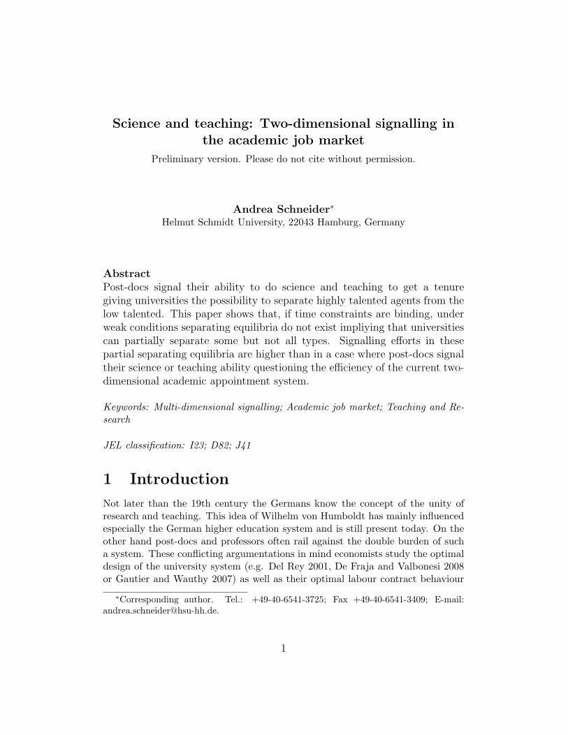
Proposition 3 If agents signal their abilities to do science (sij) and teaching(tij), universities offer wages w(sij , tij), the time constraint is binding, i.e. if inProposition 2 s∗HH + t∗HH > l, and Assumption 1 holds, there is no separatingequilibrium.If Assumption 1 does not hold the separating equilibrium from Proposition 2 isdestroyed but there is another separating equilibrium.

For an illustration of a situation where Assumption 1 holds see Figure 1.10 Thefigure describes the incentive compatibilty constraints of type HH. All strategies

9In the present model the signalling effort in the two-dimensional case is exactly thesum of the two one-dimensional signalling models where the agent signals on teaching orscience. However, this result is driven by the additive structure of productivity and costs.

10The figure refers to parameter setting θsL = 2, θs

H = θtL = 3 and θt

H = 4.

8

tHH

sHH

1

2

4

5

6

7

1 3 4 5 6 7 8 9 10 11

€

sHH∗

€

tHH∗

Figure 1: Incentive compatibility constraints for type HH when Assumption1 holds.

in the light-grey triangle prevent HH from mimicing LH and vice versa. The dark-grey triangle consists of all s-t-combinations that prevent HH from mimicing HLand vice versa. The black triangle therefore gives all strategies that fulfil both con-ditions. The strategy (s∗HH , t

∗HH) is the equilibrium strategy. The key idea here is

as follows: Because of the pure cost effect of signalling HH realises a cost minimalcombination that is tangent to the black triangle at its lower bound. The lowerbound of the light-grey triangle has a slope of −(θtH/θ

sL). The lower bound of the

dark-grey triangle has a slope of−(θtL/θsH). Since the slope ofHH’s cost function is

−(θtH/θsH) and therefore meets the condition −(θtH/θ

sL) < −(θtH/θ

sH) < −(θtL/θ

sH)

strategy (s∗HH , t∗HH) becomes the cost minimal strategy that fulfils both incentive

compatibility constraints. However, if the euqilibrium strategy of type HH, i.e.(s∗HH , t

∗HH), is unrealisable because of time constraints there is no other strategy

that fulfils the incentive compatibility constraints of type HH. So, if Assumption1 holds there is no spearating PBE.

9

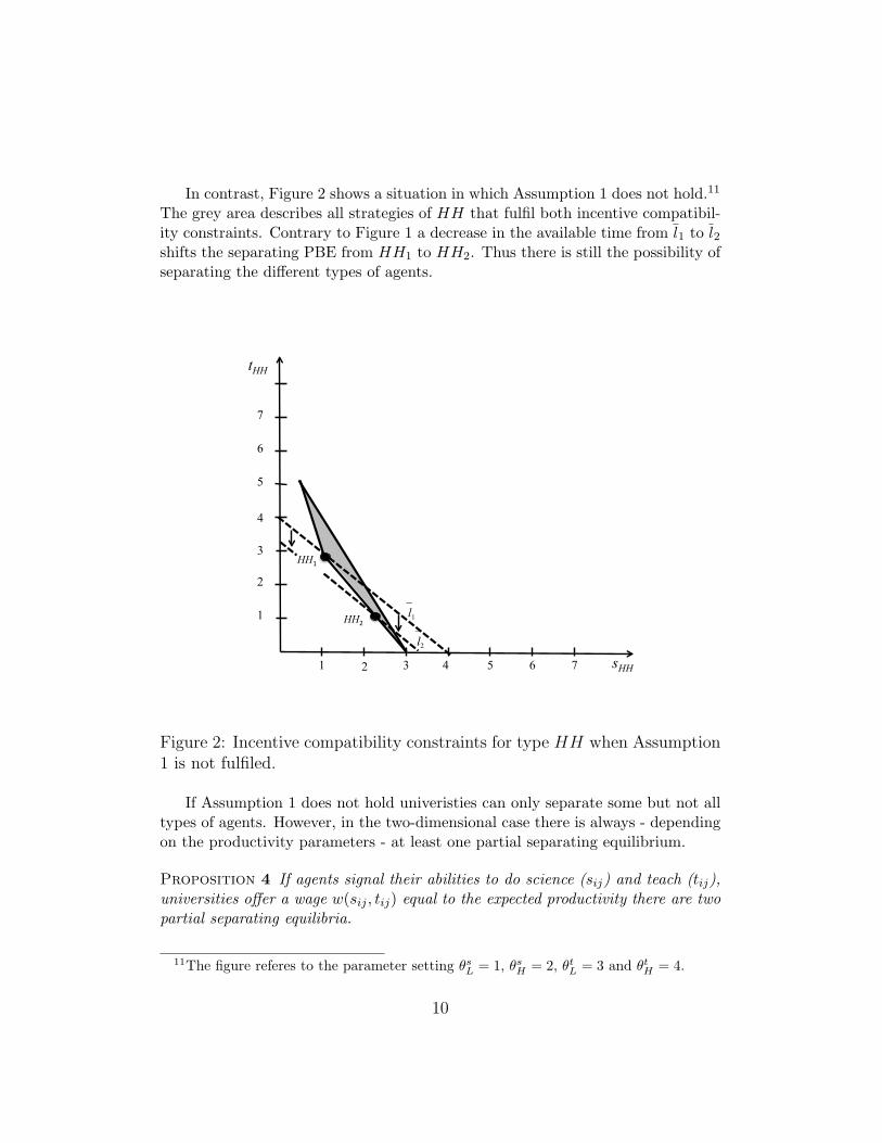
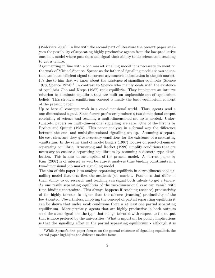
In contrast, Figure 2 shows a situation in which Assumption 1 does not hold.11

The grey area describes all strategies of HH that fulfil both incentive compatibil-ity constraints. Contrary to Figure 1 a decrease in the available time from l1 to l2shifts the separating PBE from HH1 to HH2. Thus there is still the possibility ofseparating the different types of agents.

tHH

sHH

1

2

4

5

6

7

1 3 4 5 6 7 2

3

l1

_

HH1

HH2

l2

_

Figure 2: Incentive compatibility constraints for type HH when Assumption1 is not fulfiled.

If Assumption 1 does not hold univeristies can only separate some but not alltypes of agents. However, in the two-dimensional case there is always - dependingon the productivity parameters - at least one partial separating equilibrium.

Proposition 4 If agents signal their abilities to do science (sij) and teach (tij),universities offer a wage w(sij , tij) equal to the expected productivity there are twopartial separating equilibria.

11The figure referes to the parameter setting θsL = 1, θs

H = 2, θtL = 3 and θt

H = 4.

10

If θsLθtH ≥ θsHθtL holds there is a partial PBE where strategies of the prospective

professors are:

(s∗LL, t∗LL) = (0, 0), (s∗HL, t

∗HL) = (θsL(θsH − θsL), 0) and

(s∗(LH,HH), t∗(LH,HH)) = (0, θtLC1(LH,HH))

with C1LH,HH ≡ αHHαLH+αHH

θsH − (1− αLHαLH+αHH

)θsL + θtH − θtL.

If θsHθtL ≥ θsLθtH holds there is a partial separating PBE where strategies of the

prospective professors are:

(s∗LL, t∗LL) = (0, 0), (s∗LH , t

∗LH) = (0, θtL(θtH − θtL)) and

(s∗(HL,HH), t∗(HL,HH)) = (θsLC1(HL,HH), 0)

with C1(HL,HH) = θsH − θsL + αHHαHL+αHH

θtH − (1− αHLαHL+αHH

)θtL.

In cause of clear arrangement Proposition 4 only denotes strategies of theprospective professors.12 The wage setting of the universities is for the sepa-rated types equal to the wage setting of Proposition 2. The pooled types arepaid by average productivities. Thus in the first partial separating PBE it isw(LH,HH) = αLH

αLH+αHHθsL + αHH

αLH+αHHθsH + θtH and in the second partial separating

equilibrium it is w(HL,HH) = θsH + αHLαHL+αHH

θtL + αHHαHL+αHH

θtH .The detailed proof can be found in the appendix on page 19. In the first par-tial separating PBE universities can distinguish between LL, HL and (LH,HH),i.e. they can not separate type LH from HH. In the second partial separatingPBE universities can separate LL from LH and (HL,HH) but not types HL andHH. The key arrangement of the proof of the first partial separating PBE (andanalogously of the second one) is as follows: Type LL does not signal becauseof the pure cost effect. Type HL playes his strategy from the one-dimensionalcase to prevent LL from mimicing. Then the incentive compatibility constraintsof (LH,HH) not to mimic LL or HL and vice versa are calculated. This resultsin the equilibrium strategy for (LH,HH).

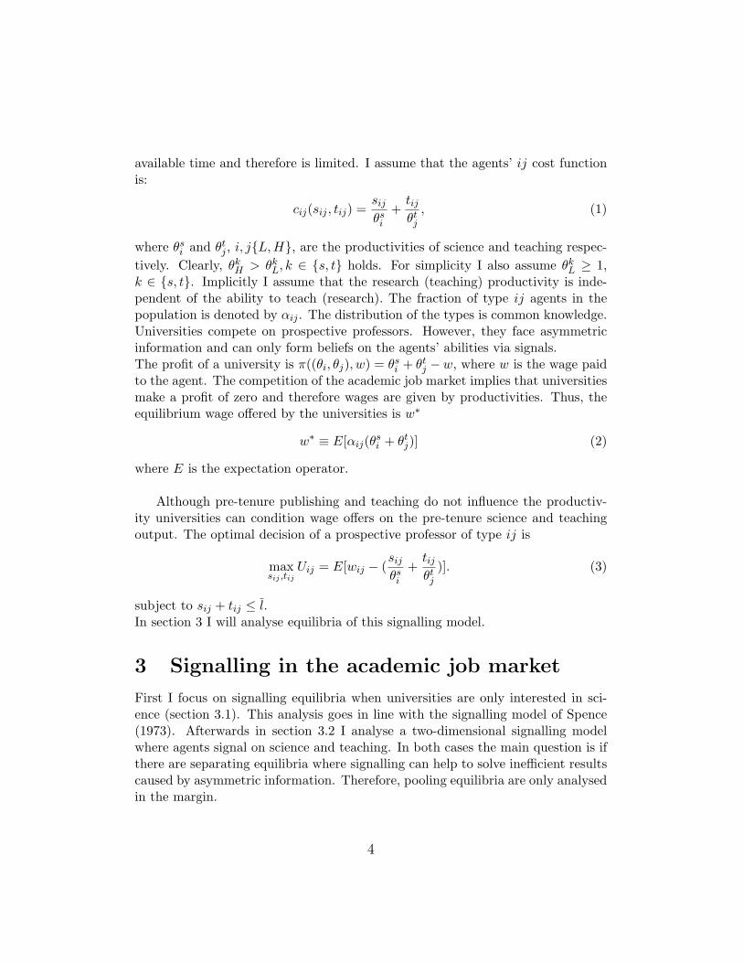
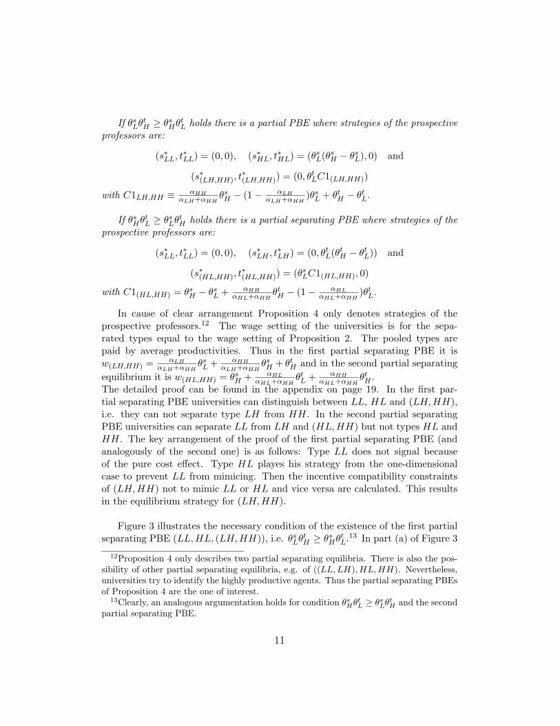
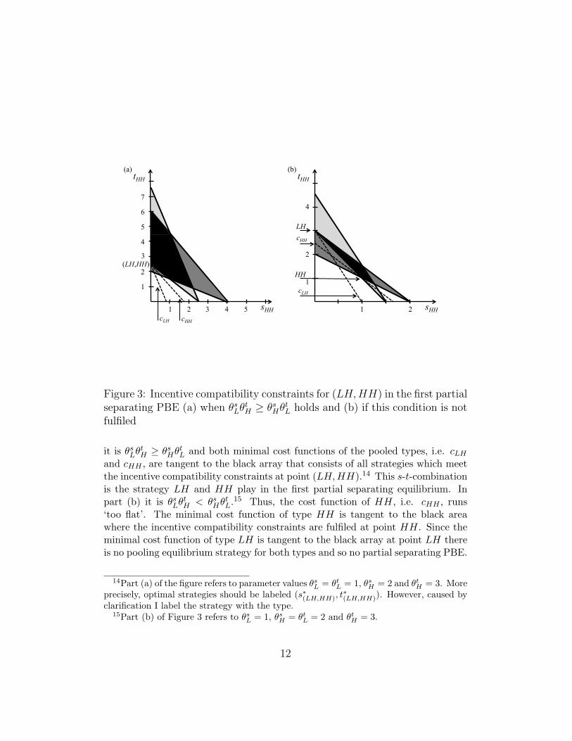
Figure 3 illustrates the necessary condition of the existence of the first partialseparating PBE (LL,HL, (LH,HH)), i.e. θsLθ

tH ≥ θsHθtL.13 In part (a) of Figure 3

12Proposition 4 only describes two partial separating equilibria. There is also the pos-sibility of other partial separating equilibria, e.g. of ((LL,LH), HL,HH). Nevertheless,universities try to identify the highly productive agents. Thus the partial separating PBEsof Proposition 4 are the one of interest.

13Clearly, an analogous argumentation holds for condition θsHθ

tL ≥ θs

LθtH and the second

partial separating PBE.

11

tHH

1

2

4

5

6

7

1 3 4 5 sHH

3

(a) (b) tHH

1

2

4

2 sHH 2 1 cLH cHH

(LH,HH)

cHH

cLH

LH

HH

Figure 3: Incentive compatibility constraints for (LH,HH) in the first partialseparating PBE (a) when θsLθ

tH ≥ θsHθ

tL holds and (b) if this condition is not

fulfiled

it is θsLθtH ≥ θsHθ

tL and both minimal cost functions of the pooled types, i.e. cLH

and cHH , are tangent to the black array that consists of all strategies which meetthe incentive compatibility constraints at point (LH,HH).14 This s-t-combinationis the strategy LH and HH play in the first partial separating equilibrium. Inpart (b) it is θsLθ

tH < θsHθ

tL.15 Thus, the cost function of HH, i.e. cHH , runs

‘too flat’. The minimal cost function of type HH is tangent to the black areawhere the incentive compatibility constraints are fulfiled at point HH. Since theminimal cost function of type LH is tangent to the black array at point LH thereis no pooling equilibrium strategy for both types and so no partial separating PBE.

14Part (a) of the figure refers to parameter values θsL = θt

L = 1, θsH = 2 and θt

H = 3. Moreprecisely, optimal strategies should be labeled (s∗(LH,HH), t

∗(LH,HH)). However, caused by

clarification I label the strategy with the type.15Part (b) of Figure 3 refers to θs

L = 1, θsH = θt

L = 2 and θtH = 3.

12

As a first result one can see that both partial separating PBE can only co-existif θsHθ

tL = θsLθ

tH holds. One example for such a situation is the symmetric case,

where low (high) productivity of science equals low (high) productivity of teaching,i.e. θsH = θtH and θsL = θtL. Thus, universities do not have a clear preference forthe one or the other output. Assuming that the highly productive agents are thecritical one and therefore normalising the productivities of the low-talented to one,i.e. θsL = θtL = 1, the first partial separating PBE only exists if teaching produc-tivity of the highly talented is higher than his research productivity. Analogously,if the contrary appraisement holds the second partial separating PBE appears. Ingeneral an angent that is good in teaching and science pooles with the type thatis highly-talented in the output that is more prefered by the universities. Thisstrengthens the argument of Becker (1975, 1979) that the professors’ research andteaching output positively react on an increase in pecuniary returns.Secondly, it is clear that without time constraints always at least one of the partialPBEs exists. However, in this case they are less interesting because the separatingPBE is more efficient. However, if time constraints are too strong even a partialseparating equilibrium maybe does not exist and only the pooling PBE where no-body signals remains.Thirdly, especially if high-talented agents are of interest signalling effort in thepartial separating equilibrium is higher than in the one-dimensional case. Theeffort of type HH in the first partial separating equilibrium is θtLC1(LH,HH) =θtL

αHHαLH+αHH

(θsH − θsL) + θtL(θtH − θtL). This is clearly higher than his effort in theone-dimensional case, i.e. higher than θtL(θtH − θtL). Thus, the partial separat-ing equilibrium requires higher signalling effort although there is no additionalinformation for the universities with respect to the type that is highly talented inscience and teaching. An analogous argumentation applies for the second partialseparating equilibrium.

4 Conclusion

The output of post-docs and professors consists, beside the administrative one thatis not mentioned here, of science and teaching. In general universities are inter-ested in both outputs and assign a tenure contract only to those post-docs that arehighly talented in both activities. However, since talent is a private informationa job market signalling model la Spence arises. Post-docs signal their ability ofscience and teaching to get a tenure.As Spence (1973) has shown in the one-dimensional case signalling can also inthe two-dimensional case separate highly talented and low talented agents. Soit solves the inefficiency problem of asymmetric information. Unfortunately, the

13

highly productive agents need a signalling effort to separate themselves from thelow-productive types and this effort increases in the two-dimensional case. Con-sidering this, time constraints attract notice.If time constraints are binding and the science (teaching) productivity of the high-talented is higher than the teaching (science) productivity of the type with lowtalent a separating equilibrium can not exist in the two-dimensional case. Therequired assumption is quite weak as it just says that universities should not pre-fer one output over the other regardless wether the first is created by a high- orlow-productive person.In addition I show that even if the separating equilibrium is destroyed by timeconstraints there is always at least one partial separating equilibrium where sometypes can be separated while others pool on the same strategy. More precisely,if the university prefers science to teaching a partial separating equilibrium existswhere universities can separate types with high or low research productivity. How-ever, they do not know if an agent with high research productivity is also highlytalented in teaching. This is the same result as in the one-dimensional case. Re-grettably, the signalling effort that only implies a pure cost effect is higher in thetwo-dimensional partial separating equilibrium than in the one-dimensional sepa-rating one. Corresponding to real life, the two-dimensional signalling system thatis currently used in academic admission processes is inefficient if time constraintsare binding. In such a situation universities can not identify both talents of hepost-doc but only one. The identifiable talent is the one they value more. Thenuniversities can ease requirements on post-docs and can let them - without loosinginformation - just signal on science or teaching.

Appendix

Proof of Proposition 2:In a separating PBE universities pay an agent ij a wage equal to his productivity.Thus, w(s∗ij , t

∗ij) = θsi + θtj holds.

This directly gives (s∗LL, t∗LL) = (0, 0) as equilibrium signal of type LL. In a

next step, signals of types HL and LH must meet the incentive compatibilityconstraints so that both types have no incentive to mimic LL and vice versa. Thisautomatically prevents HH from mimicing LL.

14

Type HL does not mimic LL if

w(s∗LL, t∗LL)− cHL(s∗LL, t

∗LL) ≤ w(sHL, tHL)− cHL(sHL, tHL)

⇔ θsL + θtL ≤ θsH + θtL −sHLθsH− tHL

θtL

⇔ 1θsH

sHL +1θtLtHL ≤ θsH − θsL

holds.Analogously, LL does not mimic HL whenever

w(s∗LL, t∗LL)− cLL(s∗LL, t

∗LL) ≥ w(sHL, tHL)− cLL(sHL, tHL)

⇔ θsL + θtL ≥ θsH + θtL −sHLθsL− tHL

θtL

⇔ 1θsLsHL +

1θtLtHL ≥ θsH − θsL

holds. Therefore the incentive compatibility constraint that prevents HL frommimicing LL and vice versa is

1θsH

sHL +1θtLtHL ≤ θsH − θsL ≤

1θsLsHL +

1θtLtHL.

A signal that maximises utility of type HL must lie on the lower bound which onecan rewrite as

sHL = θsL(θsH − θsL)−θsLθtLtHL.

Type HL will now choose the signal that fulfils this condition and minimises costs.Since costs are (taking the last equation into account)

csHL,tHL =sHLθsH

+tHLθtL

=θsL(θsH − θsL)

θsH−

θsLθsHθ

tL

tHL +1θtLtHL

=θsL(θsH − θsL)

θsH+ (1−

θsLθsH

)1θtL︸ ︷︷ ︸

>0

tHL

the minimal cost combination is t∗HL = 0 and therefore s∗HL = θsL(θsH − θsL). TypeHL’s strategy in the separating PBE is (s∗HL, t

∗HL).

15

In the same way type LH does not mimic type LL if

w(s∗LL, t∗LL)− cLH(s∗LL, t

∗LL) ≤ w(sLH , tLH)− cLH(sLH , tLH)

⇔ θsL + θtL ≤ θsL + θtH −sLHθsL− tLH

θtH

⇔ 1θsLsLH +

1θtH

tLH ≤ θtH − θtL

holds.Type LL does not mimic type LH if

w(s∗LL, t∗LL)− cLL(s∗LL, t

∗LL) ≥ w(sLH , tLH)− cLL(sLH , tLH)

⇔ θsL + θtL ≥ θsL + θtH −sLHθsL− tLH

θtL

⇔ 1θsLsLH +

1θtLtLH ≥ θtH − θtL

is fulfiled. Taking both conditions together type LH has no incentive to mimictype LL and vice versa if

1θsLsLH +

1θtH

tLH ≤ θtH − θtL ≤1θsLsLH +

1θtLtLH

holds. Again LH chooses a signal on the lower bound given by the second part ofthe condition. Thus it is

tLH = θtL(θtH − θtL)−θtLθsLsLH .

This in mind costs of type HL are given by

cLH(sLH , tLH) =sLHθsL

+tLHθtH

=θtL(θtH − θtL)

θtH+

1θsLsLH −

θtLθsLθ

tH

sLH

= (1−θtLθtH

)1θsL︸ ︷︷ ︸

>0

sLH +θtL(θtH − θtL)

θtH.

To minimise costs and therefore maximise utility given the wage θsL + θtH type LHplays s∗LH = 0 and t∗LH = θtL(θtH − θtL) in equilbrium.

16

With (s∗HL, t∗HL) and (s∗LH , t

∗LH) type HL has no incentive to mimic type LH

and vice versa cause

w(s∗LH , t∗LH)− cHL(s∗LH , t

∗LH) ≤ w(s∗HL, t

∗HL)− cHL(s∗HL, t

∗HL)

⇔ θsL + θtH −θtL(θtH − θtL)

θtL≤ θsH + θtL −

θsL(θsH − θsL)θsH

⇔ 0 ≤ (θsH − θsL)2

and

w(s∗HL, t∗HL)− cLH(s∗HL, t

∗HL) ≤ w(s∗LH , t

∗LH)− cLH(s∗LH , t

∗LH)

⇔ θsH + θtL −θsL(θsH − θsL)

θsL≤ θsL + θtH −

θtL(θtH − θtL)θtH

⇔ 0 ≤ (θtH − θtL)2

are always fulfiled.

In a last step one has to make sure that HH does neither mimic HL nor LHand vice versa. Type HH does not mimic HL whenever

w(s∗HL, t∗HL)− cHH(s∗HL, t

∗HL) ≤ w(sHH , tHH)− cHH(sHH , tHH)

⇔ θsH + θsL −θsL(θsH − θsL)

θsH≤ θsH + θtH −

sHHθsH− tHH

θtH

⇔ sHH +θsHθtH

tHH ≤ θsH(θtH − θtL) + θsL(θsH − θsL)

holds.Analogously, type HL has no incentive to mimic HH if

w(sHH , tHH)− cHL(sHH , tHH) ≤ w(s∗HL, t∗HL)− cHL(s∗HL, t

∗HL)

⇔ θsH + θtH −sHHθsH− tHH

θtL≤ θsH + θtL −

θsL(θsH − θsL)θsH

⇔ sHH +θsHθtLtHH ≥ θsH(θtH − θtL) + θsL(θsH − θsL)

is fulfiled. Both conditions together are the incentive compatibility condition thatprevents HH from mimicing HL and vice versa. Because of the pure cost effectof signalling the lower bound of the second condition, i.e.

sHH +θsHθtLtHH = θsH(θtH − θtL) + θsL(θsH − θsL)

⇔ sHH = θsH(θtH − θtL) + θsL(θsH − θsL)−θsHθtLtHH (4)

17

is a necassary condition for a separating PBE. However additionally, type HHdoes not have an incentive to mimic type LH and vice versa. Therefore,

w(s∗LH , t∗LH)− cHH(s∗LH , t

∗LH) ≤ w(sHH , tHH)− cHH(sHH , tHH)

⇔ θsL + θtH −θtL(θtH − θtL)

θtH≤ θsH + θtH −

sHHθsH− tHH

θtH

⇔θtHθsH

sHH + tHH ≤ θtH(θsH − θsL) + θtL(θtH − θtL)

and

w(sHH , tHH)− cLH(sHH , tHH) ≤ w(s∗LH , t∗LH)− cLH(s∗LH , t

∗LH)

⇔ θsH + θtH −sHHθsL− tHH

θtH≤ θsL + θtH −

θtL(θtH − θtL)θtH

⇔θtHθsLsHH + tHH ≥ θtH(θsH − θsL) + θtL(θtH − θtL)

must hold. Both condtions together are the incentive compatibility constraint thatprevent HH from mimicing LH and vice versa. Cause of the pure cost effect ofsignalling the lower bound of the second condition, i.e.

θtHθsLsHH + tHH = θtH(θsH − θsL) + θtL(θtH − θtL)

⇔ sHH = θsL(θsH − θsL) +(θtH − θtL)θsLθ

tL

θtH−θsLθtH

tHH (5)

is a necessary condition for a PBE. In a separating PBE type HH neither mim-ics HL nor LH. Thus, conditions (4) and (5) must hold. Both linear functionsdescribe the lower bound of the area that fulfils both incentive compatibility con-straints. Because of the pure cost effect of signalling the optimal strategy is elementof this lower bound. To make sure that the optimal startegy is unique the slopeof this lower bound must be unequal to the slope of the cost function of HH.16

The cost function of type HH is cHH(sHH , tHH) = (sHH/θsH) + (tHH/θtH). So,the slope of this function in a s-t-area is −(θtH/θ

sH). As the slope of equation (4)

in such an area is −(θtL/θsH) and the slope of equation (5) is −(θtH/θ

sL) there is a

unique optimal strategy of HH that is given by the point of intersection of the

16If this condition is not fulfiled the minimal cost combination would be tangent to thearea that fulfils the incentive compatibility constraints on a whole section represented bya part of the linear function (4) or (5) and not to a unique point.

18

linear combinations (4) and (5). Calculating this point of intersection leads to

θsH(θtH − θtL) + θsL(θsH − θsL)−θsHθtLtHH = θsL(θsH − θsL) +

(θtH − θtL)θsLθtL

θtH−θsLθtH

tHH

⇔ θsHθtH(θtH − θtL)− θsLθtL(θtH − θtL) =

θsHθtH − θsLθtLθtL

tHH

⇔ (θsHθtH − θsLθtL)(θtH − θtL) =

θsHθtH − θsLθtLθtL

tHH

⇔ t∗HH = θtL(θtH − θtL).

Inserting this in equation (4) gives the first part of the equilibrium signal s∗ =θsL(θsH − θsL). �

Proof of Proposition 4:The sequence of the proof of the partial separating PBE (LL,HL, (LH,HH)) isas follows:First of all I find the optimal strategy for HL that prevents him from mimicingLL. Secondly I give the incentive compatibility constraint that prevents LL frommimicing (LH,HH) and vice versa. Thirdly, I give the incentive compatibilityconstraint that prevents HL from mimicing (LH,HH) and vice versa. Step twoand three together result in an optimal strategy for (LH,HH).

In a PBE where LL is separated he has no icentive to signal. Thus, (s∗LL, t∗LL) =

(0, 0). Then refering to the first step HL signals (s∗HL, t∗HL) = (θsL(θsH − θsL), 0) to

prevent LL from mimicing him. This strategy directly results from the separatingPBE.

To make sure that in a second step LL does not mimic (LH,HH)

wLL − cLL(s∗LL, t∗LL) ≥ w(LH,HH) − cLL(s(LH,HH), t

∗(LH,HH))

⇔ θsL + θtL ≥ αLHαLH + αHH

θsL +αHH

αLH + αHHθsH + θtH

−s(LH,HH)

θsL−t(LH,HH)

θtL

⇔s(LH,HH)

θsL+t(LH,HH)

θtL≥ αHH

αLH + αHHθsH − (1− αLH

αLH + αHH)θsL + θtH − θtL︸ ︷︷ ︸

≡C1(LH,HH)

.

(6)

19

must hold.Analogously, LH and therefore (LH,HH) does not mimic LL if

wLL − cLH(s∗LL, t∗LL) ≤ w(LH,HH) − cLH(s(LH,HH),tLH,HH

)

⇔ θsL + θtL ≤ αLHαLH + αHH

θsL +αHH

αLH + αHHθsH + θtH

−s(LH,HH)

θsL−t(LH,HH)

θtH

⇔s(LH,HH)

θsL+t(LH,HH)

θtH≤ αHH

αLH + αHHθsH − (1− αLH

αLH + αHH)θsL + θtH − θtL︸ ︷︷ ︸

=C1(LH,HH)

.

is fulfiled. Since signals can not be negative a necessary condition for the existenceof the partial separating PBE is C1(LH,HH) > 0. I will come to this later on.

To prevent HL from mimicing (LH,HH) (third step) the following conditionmust hold:

wHL − cHL(s∗HL, t∗HL) ≥ w(LH,HH) − cHL(s(LH,HH), t(LH,HH))

⇔ θsH + θtL −θsL(θsH − θsL)

θsH≥ αLH

αLH + αHHθsL +

αHHαLH + αHH

θsH + θtH

−s(LH,HH)

θsH−t(LH,HH)

θtL

⇔s(LH,HH)

θsH+t(LH,HH)

θtL≥

−(1− αHHαLH + αHH

)θsH + (1 +αLH

αLH + αHH)θsL + θtH − θtL −

(θsL)2

θsH︸ ︷︷ ︸≡C2(LH,HH)

(7)

Analogously, to prevent HH and therefore (LH,HH) from mimicing HL

wHL − cHH(s∗HL, t∗HL) ≤ w(LH,HH) − cHH(s(LH,HH), t(LH,HH))

⇔ θsH + θtL −θsL(θsH − θsL)

θsH≤ αLH

αLH + αHHθsL +

αHHαLH + αHH

θsH + θtH

−s(LH,HH)

θsH−t(LH,HH)

θtH

⇔sLH,HHθsH

+t(LH,HH)

θtH≤

20

−(1− αHHαLH + αHH

)θsH + (1 +αLH

αLH + αHH)θsL + θtH − θtL −

(θsL)2

θsH︸ ︷︷ ︸=C2(LH,HH)

must hold. A necessary condition for the existence of the partial separating PBEis again that C2(LH,HH) > 0 is fulfiled. This condition is even stronger thanC1(LH,HH) from above because

C2(LH,HH) − C1(LH,HH) = −θsH + 2θsL −(θsL)2

θsH

=−(θsH)2 + 2θsHθ

sL − (θsL)2

θsH

= −(θsH − θsL)2

θsH< 0

holds. Although C2(LH,HH) < C1(LH,HH) is fulfiled one can not directly see ifequation (6) or equation (7) is the stronger condition because of the differentLHS. If you compare both conditions you find that the relationship depends onthe exact parameter values. However, I show that the optimal - cost minimal -behavior for type LH and HH is the same regardless whether equation (6) orequation (7) is the stronger condition.

Thus assume that equation (6) is stronger than equation (7) then t(LH,HH) =

θtLC1(LH,HH) −θtLθsLs(LH,HH) holds. This in mind costs of LH are

s(LH,HH)

θsL+t(LH,HH)

θtH=

1θsL

(1−θtLθtH

)︸ ︷︷ ︸>0

s(LH,HH) +θtLθtH

C1(LH,HH).

Since costs increase in s(LH,HH) the optimal strategy of LH is s(LH,HH) = 0.Analogously, costs of HH are

s(LH,HH)

θsH+t(LH,HH)

θtH= (

1θsH−

θtLθsLθ

tH

) +θtLθtH

C1(LH,HH).

If 1θsH− θt

L

θsLθ

tH≤ 0 holds the optimal strategy is to maximise s(LH,HH). However,

then the partial separating PBE is destroyed. Type LH and HH do not play thesame strategy. Therefore 1

θsH− θt

L

θsLθ

tH≥ 0 must hold to ensure the described PBE.

If equation (6) is the stronger condition one θsLθtH ≥ θsHθ

tL becomes a necessary

condition of the partial separating PBE.

21

Now assume that instead of equation (6) equation (7) is the stronger conditionthen t(LH,HH) = θtLC2(LH,HH) −

θtLθsHs(LH,HH) holds and costs of type LH are

s(LH,HH)

θsL+t(LH,HH)

θtH= (

1θsL−

θtLθsHθ

tH

)s(LH,HH) +θtLθtH

C2(LH,HH)

= (θsHθ

tH − θsLθtLθsHθ

tLθ

tH

)︸ ︷︷ ︸>0

s(LH,HH) +θtLθtH

C2(LH,HH).

Again it is optimal for type LH to play s(LH,HH) = 0. Analogously, costs of typeHH are

s(LH,HH)

θsH+t(LH,HH)

θtH=

1θsH

(1−θtLθtH

)s(LH,HH) +θtLθtH

C2(LH,HH).

As costs increase in s(LH,HH) type HH sets s(LH,HH) = 0.

Summarising, under both assumption s∗(LH,HH) = 0 is an optimal strategy forboth pooling types. This reduces condition (6) to t(LH,HH) = θtLC1LH,HH and con-dition (7) to t(LH,HH) = θtLC2(LH,HH). With C1(LH,HH) > C2(LH,HH) from theabove condition (6) becomes the crucial condition for the existence of the partialseparating PBE. The equilibrium strategy of (LH,HH) is (s∗(LH,HH), t

∗(LH,HH)) =

(0, θtLC1(LH,HH)). A necessary condition for the existence of the equilibrium isθsLθ

tH > θsHθ

tL.

Finally, the proof of the second partial PBE, i.e. of (LL,LH, (HL,HH)) isanalogous and is therefore not specified here. �

References

Allgood, Sam and Wiliam B. Walstad (2005). Views of teaching and researchin economics and other disciplines. American Economic Review Papers andProceedings 95 (2), 177–183.

Armstrong, Mark and Jean-Charles Rochet (1999). Multi-dimensional screening:A user’s guide. European Economic Review 43 , 959–979.

Becker, William E. (1975). The university professor as a utility maxi-mizer and producer of learning, research, and income. Journal of HumanRessources 10 , 109–115.

22

Becker, William E. (1979). Professorial behavior given a stochastic reward struc-ture. The American Economic Review 69 (5), 1010–1017.

Becker, William E. and Peter E. Kennedy (2005). Does teaching enhance re-search in economics? American Economic Review Papers and Proceed-ings 95 (2), 172–176.

Cho, In-Koo and David M. Kreps (1987). Signaling games and stable equilibria.The Quarterly Journal of Economics 102 (2), 179–221.

De Fraja, Gianni and Paola Valbonesi (2008). The design of the universitysystem. CEPR Discussion Paper no. 7038.

Del Rey, Elena (2001). Teaching versus research: A model of state universitycompetition. Journal of Urban Economics 49 , 356–373.

Engers, Maxim (1987). Signalling with many signals. Econometrica 55 (3), 663–674.

Gautier, Axel and Xavier Wauthy (2007). Teaching versus research: The roleof internal financing rules in multi-department univeristies. European Eco-nomic Review 51 , 273–295.

Gottlieb, Esther E. and Bruce Keith (1997). The academic research-teachingnexus in eight advanced-industrialized countries. Higher Education 34 , 397–420.

Hattie, John and H. W. Marsh (1996). The relationship between research andteaching: A meta-analysis. Review of Educational Research 66 (4), 507–542.

Kim, Jeong-Yoo (2007). Multidimensional signaling in the labor market. Manch-ester School 75 (1), 64–87.

Mitchell, John E. and Douglas S. Rebne (1995). Nonlinear effects of teachingand consulting on academic research productivity. Socio-Economic PlanningSciences 29 (1), 47–57.

Rochet, Jean-Charles and Martine Qunizii (1985). Multidimensional signalling.Journal of Mathematical Economics 14 , 261–284.

Spence, Michael (1973). Job markt signalling. The Quarterly Journal of Eco-nomics 87 (3), 355–374.

Spence, Michael (1974). Competitive and optimal responses to signals: An anal-ysis of efficiency and distribution. Jounral of Economic Theory 7 , 296–332.

Walckiers, Alexis (2008). Multi-dimensional contracts with task-specific pro-ductivity: An application to universities. International Tax and Public Fi-nance 15 , 165—198.

23