Embed Size (px)
Citation preview

35
Chapter-3
ROUGH SET THEORY AND REDUCT
BASED RULE GENERATION
3.1 Introduction
Rough Set Theory (RST), proposed in 1982 by Zdzislaw Pawlak, is since then in a state
of constant development. Its methodology is concerned with the classification and
analysis of imprecise, uncertain or incomplete information and knowledge, and has been
considered as one of the first non-statistical approaches in data analysis [107]. The
fundamental concept behind RST is the approximation of lower and upper spaces of a set,
the approximation of spaces being the formal classification of knowledge regarding the
interest domain. The subset generated by lower approximations is characterized by
objects that will definitely form part of an interest subset, whereas the upper
approximation is characterized by objects that will possibly form part of an interest
subset. Every subset defined through upper and lower approximation is known as Rough
Set [107]. Over the years RST has become a valuable tool in the resolution of various
problems, such as representation of uncertain or imprecise knowledge; knowledge
analysis; evaluation of quality and availability of information with respect to consistency
and presence of data patterns; identification and evaluation of data dependency and
reasoning based on uncertain and reduct of information data [105].
The extent of rough set applications used today is much wider than in the past, principally
in the areas of medicine, analysis of database attributes and process control. RST has
some overlaps with other methods of data analysis, e.g., statistics, cluster analysis, fuzzy
sets, evidence theory and others but it can be viewed in its own rights as an independent
discipline [114]. The rough set approach seems to be of fundamental importance to AI
and cognitive sciences, especially in the areas of machine learning, knowledge
acquisition, decision analysis, knowledge discovery from databases, expert systems,
36
inductive reasoning and pattern recognition. It seems of particular importance to decision
support systems and data mining [103]. This theory has been successfully applied in
many real-life problems in medicine, pharmacology, engineering, banking, financial and
market analysis and others [115].
An early application of this theory was to classify imprecise and incomplete information.
Reduct and Core are the two important concepts in rough sets theory. RST is an elegant
theory when applied to small data sets because it can always find the minimal reduct and
generate minimal rule sets. However, the general solution for finding the minimal reduct
is NP-hard [78]. An NP-hard problem is defined as a problem that cannot be solved in
polynomial time. In other words as data sets grow large both in dimension and volume
then finding the minimal reduct becomes computationally infeasible.
Rough sets approach shows many advantages. The most important ones are [115].
Synthesis of efficient algorithms for finding hidden patterns in data;
Identification of relationships that would not be found using statistical methods;
Representation and processing of both qualitative and quantitative parameters and
mixing of user-defined and measured data;
Reduction of data to a minimal representation (data reduction);
Evaluation of the significance of data;
Synthesis of classification or decision rules from data;
Legibility and straightforward interpretation of synthesized models;
Generates sets of decision rules from data;
• It is easy to understand;
• Offers straightforward interpretation of obtained results;
So rough set theory can be very useful in many intelligent industrial applications as an
independent approach or combined together with other areas of soft computing, e.g.
fuzzy sets, neural networks, logistic regression etc.

37
3.2 Basic Philosophy of Rough Set
In this section, all the important concepts related to Rough sets theory have been defined
[106].
3.2.1 Equivalence Relation
Let U be a non-empty set and let p, q, and r be elements of U. Consider R such that pRq
if and only if (p, q) is in R. R is an equivalence relation if it satisfies the following three
properties:
i) Reflexive Property: (p, p) is in R for all p in U.
ii) Symmetric Property: if (p, q) is in R, then (q, p) is in R.
iii) Transitive Property: if (p, q) and (q, r) are in R, then (p, r) is in R.
3.2.2 Decision Table or Information System and Indiscernibility Relation
Let T = (U, A, Q, ρ) be a Information system, where U is a non-empty finite set of
objects called the universe, A is a set of attributes, Q is the union of domains of attributes
in A and ρ : U X Q A is a total description function. For classification of objects, set
of attributes A is divided into condition attributes denoted by CON and decision attribute
denoted by DEC. In the context of classification the information table is known as
decision table. The elements of U are called objects, cases, instances or observations[110].
Attributes are interpreted as features, variables or characteristic conditions. Given a
feature a, such that:
a :U Va for a A, Va is called the value set of a .
Let a A, P A, the indiscernibility relation IND(P), is defined as:
IND(P) = {(x, y)U U : for all a P, a(x) = a( y)} In simple words, two objects are
indiscernible if we can not differentiate between them, because they do not differ enough
on the subset P of attributes.
3.2.3 Lower Approximation of a Subset
Let B C and X U , the B-lower approximation set of X, is the set of all elements
of U which can be with certainty classified as elements of X.
XxBUxXB )(:)(

38
This is the B-lower approximation of the subset of X.
3.2.4 Upper Approximation of a Subset
The B-upper approximation set of X is the set of all element of U, that can possibly
belong to the subset of interest X [111].
This represents the B-upper approximation of the subset of X.
3.2.5 Boundary Region of a Subset
It is the collection of elementary sets defined by:
Boundary region consists of those objects that we cannot decisively classify into X in B.
3.2.6. Rough Set
A subset defined through its lower and upper approximations is called a Rough Set.
When the boundary region is a non-empty set that is )(XB ≠ )(XB then the set is
called a Rough Set.
3.2.7 Crisp Set.
A set is called Crisp set when its boundary region is empty that is )(XB = )(XB
3.2.8 Positive Region of a Subset
It is the set of all objects from the universe U which can be classified with certainty to
classes of U / D employing attributes from C.
CPOS )(D = )(XC
XxBUxXB )(:)(
)()()( XBXBXBNB

39
Where )(XC denotes the lower approximation of the set X with respect to C. The
positive region of the subset X belonging to the partition U/D is also called the lower
approximation of the set X. The positive region of a decision attribute with respect to a
subset C represents approximately the quality of C. The union of the positive and the
boundary regions constitutes the upper approximation [109].
Definition 3.2.9 Negative Region of a Subset
The negative region consists of those elementary sets that have no predictive power for a
subset X given a concept R. They consist of all classes that have no overlap with the
concept. That is,
RNEG )(X = )(XRU
3.2.10. Reduct
A system T = (U, A, C, D) is independent if all c in C are indispensable. A set of features
R C is called the reduct of C if T'= (U, A, R, D) is independent and
POSR (D) = POSC (D). Furthermore, there is no T R such that
POST (D) = POSC (D)
A Reduct is a minimal set of features that preserves the indiscernibility relation produced
by a partition of C. There could be several subsets of attributes like R. Similar or
indiscernible objects may be represented several times on an information table, some of
the attributes maybe superfluous or irrelevant, and they could be removed without loss of
classification performance [140].
3.2.11 Core
The set of all the features indispensable in C is denoted by CORE(C). We have
CORE(C) = RED(C)
Where RED(C) is the set of all reducts of C. Thus, the Core is the intersection of all
reducts of an information system [112]. The Core does not consider the dispensable
features and it can be expanded using Reducts.

40
3.2.12. The Dependency Coefficient
Let T = (U, A, C, D) be a decision table. The Dependency Coefficient between the
condition attributes C, and the decision attribute D is given by
γ(C,D) = |POSC(D)| / |U|
The dependency coefficient varies between 0 and 1, since it expresses the proportion of
the objects correctly classified with respect to the total, considering the conditional
features set. If γ = 1, D depend totally on C, if 0<γ<1, the D depends partially on C, and
if γ = 0, then D does not depend on C [113]. A decisional attribute depends on the set of
conditional features if all values of decisional feature D are uniquely determined by
values of conditional attributes; that is there exist a dependency between values of
decisional and conditional features.
3.2.13 Accuracy of the Approximation
The accuracy of the approximation of the set X from the elementary subsets is measured
as the ratio of the lower and the upper approximation size. The ratio is equal to 1, if no
boundary region exists, which indicates a perfect classification. In this case, deterministic
rules for the data classification can be generated [112].
α(X) = Lower(X) / Upper(X)
Thus, a set X with accuracy equal to 1 is crisp, otherwise X is rough. Obviously 0 α
1.
3.2.14 Significance of Attributes
One of the first ideas was to consider the relevant features in the core of an information
system, i.e. the features that belong to the intersection of all reducts of the information
system [108]. It can be easily checked that several definitions of relevant features that are
used by machine learning community can be interpreted by choosing a relevant decision
system corresponding to the given information system [9].
It is also possible to find the relevant features from some approximate reducts of
sufficiently high quality. In attribute reduction some of the attributes can be eliminated
from the information table without loosing relevant information contained in the table [8].
The idea of attribute reduction can be generalized by an introduction of the concept of

41
significance of attributes, which enables an evaluation of attributes not only by a two-
valued scale, {dispensable , indispensable} but by associating with an attribute a real
number from the [0,1] closed interval; this number expresses the importance of the
attribute in the information table.
Let C and D be the sets of condition and decision attributes respectively and let a be a
condition attribute, i.e., Ca . As indicated earlier the number ),( DC expresses the
degree of consistency of the decision table, or the degree of dependency between
attributes C and D, or accuracy of approximation of U/D by C. We can ask how the
coefficient ),( DC changes when removing the attribute a, i.e., what is the difference
between ),( DC and )},{( DaC . We can normalize the difference and define the
significance of the attribute a as
),(
)},{(1
),(
))},{(),(()(),(
DC
DaC
DC
DaCDCaDC
,
Where C and D are condition and decision attributes respectively. In general we have
1)(0 a , for any sets of C and D.
3.3 Information System of a Patient Dataset
A data set is represented as a decision table, where each row represents a case, an event, a
patient, or simply an object. Every column represents an attribute (a variable, an
observation, a property, etc.) and its value for different objects. The attribute values may
be supplied by human expert or user. This table is called an information system or
decision table [159].
A decision table is used to specify what conditions lead to decisions. A decision table is
defined as T = (U, A, Q, ρ) where U is the set of objects in the table, A is a set of
attributes, Q is the union of domains of attributes in A and ρ : U X C A is a total
description function. For classification of objects, set of attributes A is divided into
condition attributes denoted by CON and decision attribute denoted by DEC and A =
CON DEC and CON ∩ DEC = φ [58]. In order to take an example we have collected
the data of 15 patients from a hospital as shown in table 3.1. Patients may or may not
have heart problem depending on the values of condition attributes. There are seven

42
condition attribute and one decision attribute. Each condition attribute has some value
from the domain of that particular attribute.
Let B = { P1, P2, P3, P4, P5, P6, P7, P8, P9, P10, P11, P12, P13, P14, P15} be the set
of 15 patients.
The set of Condition attributes of Information System C = {Heart Palpitation, Blood
Pressure, Chest Pain, Cholesterol, Fatigue, Shortness of Breath, Rapid Weight Gain}
The set of Decision attribute of information system D = {Heart Problem}
Patient H.P. B.P. C.P. Cholesterol Fatigue S.O.B Rapid
Weight
Gain
Heart
Problem
Decision
P1 High High High Normal Low Low High Yes
P2 Low Low High Normal Low Normal Low No
P3 Low High Low Low Normal Low Low No
P4 V_high Low V_high Low Low Normal High Yes
P5 High High V_high Low Low Low High Yes
P6 Low High Low High Low Normal Low No
P7 High High V_high Low Low Low High Yes
P8 High High High Low Low Low High Yes
P9 High High High Low Low Low High No
P10 V_high Low V_high Low Low Normal High Yes
P11 V_high High High Low Normal Normal High Yes
P12 V_high Low High Low Low Low High Yes
P13 High Low Low Low High Low Low No
P14 Low Low High High Low High Low No
P15 High V_high V_high Normal Low Normal High Yes
Table 3.1 Information System or Patient Data Set of 15 Patients

43
Table 3.2 represents the set of values for each condition attribute of the information table
3.1. This table represents the nominal values of patient dataset.
Attributes Nominal Values
Condition Attributes
Heart Palpitation,
Blood Pressure
Chest Pain,
Cholesterol,
Fatigue,
Shortness of Breath,
Rapid Weight Gain,
High, Low, V_high
High, Low, V_high
High, Low, V_high
Normal, High, Low
Normal, High, Low
Normal, High, Low
High, Low
Decision Attribute Heart Problem Yes, No
Table 3.2 Values of Patient Dataset
The Heart Problem of a patient is related to the Heart Palpitation, Blood Pressure, Chest
Pain, Rapid Weight Gain, Fatigue, Shortness of Breath, and Cholesterol. Table 3.1 can
be used to decide whether a patient has heart problem or not according to various values
of its condition attributes (Heart Palpitation, Blood Pressure, Chest Pain, Rapid Weight
Gain, Fatigue, Shortness of Breath, and Cholesterol). For example, the first row of this
table specifies that a patient with Heart Palpitation = High, Blood Pressure = High,
Chest Pain= High, Cholesterol = Normal, Fatigue = Low, Shortness of Breath = Low and
Rapid Weight Gain = High, then Heart Problem= Yes.
The rows in this table are called the objects, and the columns in this table are called
attributes [107]. Condition attributes are the features of a patient related to its Heart
Problem.
There are 15 patients in this dataset, and there are no missing attribute values. The
situation when some of the condition attributes have missing values has not been
discussed here. The reduct and the core are important concepts in rough sets theory. A
reduct is a subset of condition attributes that are sufficient to classify the decision table. A

44
reduct may not be unique. The core is contained in all the reduct sets, and it is the
necessity of the whole data. In other words, any reduct generated from the original data
set cannot exclude the core attributes.
3.4 Indiscernible Relation of the Patient Dataset
Indiscernible Relation is a central concept in RST, and is considered as a relation
between two or more objects, where all the values are identical in relation to a subset of
considered attributes. Indiscernible relation is an equivalence relation, where all identical
objects of set are considered as the elementary sets [112].
It can be observed from table 3.1 that the set is composed of attributes that are directly
related to patients symptoms = {Heart Palpitation, Blood Pressure, Chest Pain,
Cholesterol , Fatigue, Shortness of Breath, Rapid Weight Gain}, the indiscernibility
relation of condition attribute is given by IND(C). When table 3.1 is broken down it can
be seen that indiscernibility relation is given in relationship to conditional attributes. The
indiscernible relations for all the conditions and decision attribute are shown from table
3.3 to table 3.11.
The Heart Palpitation attribute generates three indiscernible elementary sets because this
condition attribute has three values ‘High’, ‘Low’ and ‘V-high’.
IND ({Heart Palpitation}) = {{P1, P5, P7, P8, P9, P13, P15}, {P4, P10, P11, P12},
{P2, P3, P6, P14}}
45
Patient H.P. B.P. C.P. Cholesterol FT S.O.B R.W.G Heart
Problem
Decision
P1 High High High Normal Low Low High Yes
P5 High High V_high Low Low Low High Yes
P7 High High V_high Low Low Low High Yes
P8 High High High Low Low Low High Yes
P9 High High High Low Low Low High No
P13 High Low Low Low High Low Low No
P15 High V_high V_high Normal Low Normal High Yes
P4 V_high Low V_high Low Low Normal High Yes
P10 V_high Low V_high Low Low Normal High Yes
P11 V_high High High Low Normal Normal High Yes
P12 V_high Low High Low Low Low High Yes
P2 Low Low High Normal Low Normal Low No
P3 Low High Low Low Normal Low Low No
P6 Low High Low High Low Normal Low No
P14 Low Low High High Low High Low No
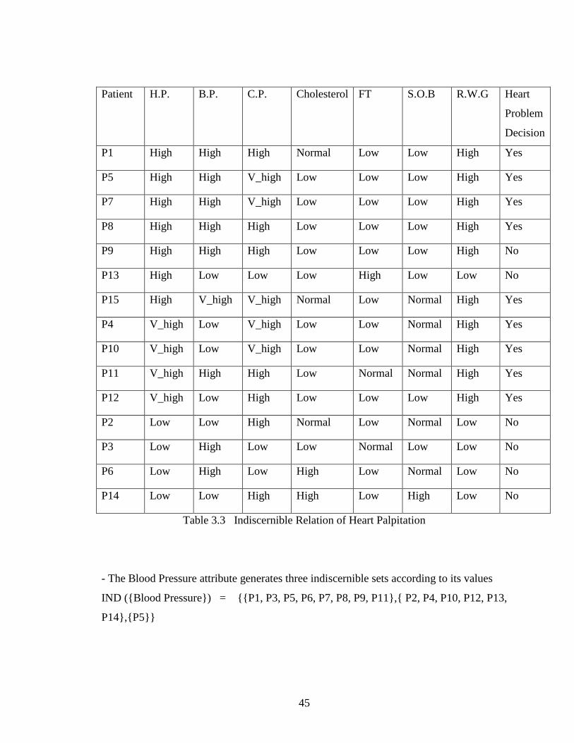
Table 3.3 Indiscernible Relation of Heart Palpitation
- The Blood Pressure attribute generates three indiscernible sets according to its values
IND ({Blood Pressure}) = {{P1, P3, P5, P6, P7, P8, P9, P11},{ P2, P4, P10, P12, P13,
P14},{P5}}

46
Patient H.P. B.P. C.P. Cholesterol FT S.O.B R.W.G Heart
Problem
Decision
P1 High High High Normal Low Low High Yes
P3 Low High Low Low Normal Low Low No
P5 High High V_high Low Low Low High Yes
P6 Low High Low High Low Normal Low No
P7 High High V_high Low Low Low High Yes
P8 High High High Low Low Low High Yes
P9 High High High Low Low Low High No
P11 V_high High High Low Normal Normal High Yes
P2 Low Low High Normal Low Normal Low No
P4 V_high Low V_high Low Low Normal High Yes
P10 V_high Low V_high Low Low Normal High Yes
P12 V_high Low High Low Low Low High Yes
P13 High Low Low Low High Low Low No
P14 Low Low High High Low High Low No
P15 High V_high V_high Normal Low Normal High Yes
Table 3.4 Indiscernible Relation of Blood Pressure
- The Chest Pain attribute generates three indiscernible elementary sets:
IND ({Chest Pain}) = {{P1, P2, P8, P9, P11, P12, P14}, {P3, P6, P13}, { P4, P5, P7,
P10, P15}}

47
Patient H.P. B.P. C.P. Cholesterol FT S.O.B R.W.G Heart
Problem
Decision
P1 High High High Normal Low Low High Yes
P2 Low Low High Normal Low Normal Low No
P8 High High High Low Low Low High Yes
P9 High High High Low Low Low High No
P11 V_high High High Low Normal Normal High Yes
P12 V_high Low High Low Low Low High Yes
P14 Low Low High High Low High Low No
P3 Low High Low Low Normal Low Low No
P6 Low High Low High Low Normal Low No
P13 High Low Low Low High Low Low No
P4 V_high Low V_high Low Low Normal High Yes
P5 High High V_high Low Low Low High Yes
P7 High High V_high Low Low Low High Yes
P10 V_high Low V_high Low Low Normal High Yes
P15 High V_high V_high Normal Low Normal High Yes
Table 3.5 Indiscernible Relation of Chest Pain
- The Cholesterol attribute generates three indiscernible elementary sets:
IND ({Cholesterol}) = {{P1, P2, P15}, {P3, P4, P5, P7, P8, P9, P10, P11, P12,
P13},{ P6, P14}}

48
Patient H.P. B.P. C.P. Cholesterol FT S.O.B R.W.G Heart
Problem
Decision
P1 High High High Normal Low Low High Yes
P2 Low Low High Normal Low Normal Low No
P15 High V_high V_high Normal Low Normal High Yes
P3 Low High Low Low Normal Low Low No
P4 V_high Low V_high Low Low Normal High Yes
P5 High High V_high Low Low Low High Yes
P7 High High V_high Low Low Low High Yes
P8 High High High Low Low Low High Yes
P9 High High High Low Low Low High No
P10 V_high Low V_high Low Low Normal High Yes
P11 V_high High High Low Normal Normal High Yes
P12 V_high Low High Low Low Low High Yes
P13 High Low Low Low High Low Low No
P6 Low High Low High Low Normal Low No
P14 Low Low High High Low High Low No
Table 3.6 Indiscernible Relation of Cholesterol
- The Fatigue attribute generates three indiscernible elementary sets because this
condition attribute assumes three values.
IND ({Fatigue}) = {{P1, P2, P4, P5, P6, P7, P8, P9, P10, P12, P14, P15}, {P3,
P11},{ P13}}

49
Patient H.P. B.P. C.P. Cholesterol FT S.O.B R.W.G Heart
Problem
Decision
P1 High High High Normal Low Low High Yes
P2 Low Low High Normal Low Normal Low No
P4 V_high Low V_high Low Low Normal High Yes
P5 High High V_high Low Low Low High Yes
P6 Low High Low High Low Normal Low No
P7 High High V_high Low Low Low High Yes
P8 High High High Low Low Low High Yes
P9 High High High Low Low Low High No
P10 V_high Low V_high Low Low Normal High Yes
P12 V_high Low High Low Low Low High Yes
P14 Low Low High High Low High Low No
P15 High V_high V_high Normal Low Normal High Yes
P3 Low High Low Low Normal Low Low No
P11 V_high High High Low Normal Normal High Yes
P13 High Low Low Low High Low Low No
Table 3.7 Indiscernible Relation of Fatigue
- The Shortness of Breath attribute generates three indiscernible elementary sets:
IND ({Shortness of Breath }) = {{P1,P3, P5, P5, P7, P8, P9, P12, P13}, {P2, P4, P6,
P10, P11, P15},{ P14}}

50
Patient H.P. B.P. C.P. R.W.G FT S.O.B Cho Heart
Problem
Decision
P1 High High High Normal Low Low High Yes
P3 Low High Low Low Normal Low Low No
P5 High High V_high Low Low Low High Yes
P7 High High V_high Low Low Low High Yes
P8 High High High Low Low Low High Yes
P9 High High High Low Low Low High No
P12 V_high Low High Low Low Low High Yes
P13 High Low Low Low High Low Low No
P2 Low Low High Normal Low Normal Low No
P4 V_high Low V_high Low Low Normal High Yes
P6 Low High Low High Low Normal Low No
P10 V_high Low V_high Low Low Normal High Yes
P11 V_high High High Low Normal Normal High Yes
P15 High V_high V_high Normal Low Normal High Yes
P14 Low Low High High Low High Low No
Table 3.8 Indiscernible Relation of Shortness of Breath
- The Rapid Weight Gain attribute generates two indiscernibility elementary sets:
IND ({Rapid Weight Gain}) = {{P1, P4, P5, P7, P8, P9, P10, P11, P12, P15}, { P2,
P3, P6, P13, P14}}

51
Patient H.P. B.P. C.P. Cholesterol FT S.O.B R.W.G Heart
Problem
Decision
P1 High High High Normal Low Low High Yes
P4 V_high Low V_high Low Low Normal High Yes
P5 High High V_high Low Low Low High Yes
P7 High High V_high Low Low Low High Yes
P8 High High High Low Low Low High Yes
P9 High High High Low Low Low High No
P10 V_high Low V_high Low Low Normal High Yes
P11 V_high High High Low Normal Normal High Yes
P12 V_high Low High Low Low Low High Yes
P15 High V_high V_high Normal Low Normal High Yes
P2 Low Low High Normal Low Normal Low No
P3 Low High Low Low Normal Low Low No
P6 Low High Low High Low Normal Low No
P13 High Low Low Low High Low Low No
P14 Low Low High High Low High Low No
Table 3.9 Indiscernible Relation of Cholesterol
- The Decision attribute generates two indiscernible elementary sets one is for decision
value ‘Yes’ and other is for decision value ‘No’.
IND ({Heart Problem}) = {{P1, P4, P5, P7, P8, P10, P11, P12, P15},{ P2, P3, P6, P9,
P13, P14}}

52
Patient H.P. B.P. C.P. Cholesterol FT S.O.B R.W.G Heart
Problem
Decision
P1 High High High Normal Low Low High Yes
P4 V_high Low V_high Low Low Normal High Yes
P5 High High V_high Low Low Low High Yes
P7 High High V_high Low Low Low High Yes
P8 High High High Low Low Low High Yes
P10 V_high Low V_high Low Low Normal High Yes
P11 V_high High High Low Normal Normal High Yes
P12 V_high Low High Low Low Low High Yes
P15 High V_high V_high Normal Low Normal High Yes
P2 Low Low High Normal Low Normal Low No
P3 Low High Low Low Normal Low Low No
P6 Low High Low High Low Normal Low No
P9 High High High Low Low Low High No
P13 High Low Low Low High Low Low No
P14 Low Low High High Low High Low No
Table 3.10 Indiscernible Relation of the Decision/ Heart Problem

53
3.5 Approximations of the Patient Dataset
The starting point of RST is the indiscernible relation, generated by information
concerning objects of interest. The indiscernible relation is intended to express the fact
that due to the lack of knowledge it is unable to discern some objects employing the
available information [111]. Approximation is also an important concept in RST;
topological operations are associated with the meaning of the approximations. The lower
and the upper approximations of a set are interior and closure operations in a topology
generated by the indiscernibility relation as described below.
a. Lower Approximation (B”)
Lower Approximation is a description of the domain objects that are known with
certainty to belong to the subset of interest. The Lower Approximation Set of a set X,
with regard to R is the set of all of objects, which certainly can be classified in X
regarding R, and is denoted by B”.
b. Upper Approximation (B*)
Upper Approximation is a description of the objects that possibly belong to the subset of
interest. The Upper Approximation Set of a set X regarding R is the set of all the objects
which can possibly be classified in X regarding R, and is denoted by B*.
c. Boundary Region (BR)
Boundary Region is description of the objects of a set X regarding R containing all the
objects, which can neither be classified as X nor as ⌐X regarding R. If the boundary
region is a null set, then the set X is considered "Crisp", that is, exact in relation to R,
otherwise, if the boundary region is not empty then the set X is consider as "Rough Set".
In that case the boundary region is BR = B* - B”.
Lower Approximation of Patient Dataset (B”)
Lower Approximation set (B”) is the set of the patients that definitely have Heart
Problem. These patients are identified as
B” = {P1, P4, P5, P7, P10, P11, P12, P15}

54
Lower Approximation set (B”) of patients that certainly do not have Heart Problem are
identified as
B” = {P2, P3, P6, P13, P14}
Upper Approximation of Patient Dataset B*
Upper Approximation set (B*) of the patients that possibly have Heart Problem are
identified as
B* = {P1, P4, P5, P7, P8, P9, P10, P11, P12, P15}
Upper Approximation set (B*) of the patients that possibly do not have Heart Problem
are identified as
B* = {P2, P3, P6, P8, P9, P13, P14}
Boundary Region of Patient Dataset (BR)
Boundary Region (B*) of the patients that do not have Heart problem are identified as:
BR = { P2, P3, P6, P8, P9, P13, P14} - { P2 ,P3 ,P6, P13, P14} = {P8, P9}.
Boundary Region (B*), the set of the patients that have Heart Problem are identified as:
BR = { P1, P4, P5, P7, P8, P9, P10, P11, P12, P15} - { P1, P4, P5, P7, P10,P11, P12,
P15} = {P8, P9}

55
Fig 3.1 Lower and Upper approximations of the Patients with Heart Problem
P1,P4,P5,P7,P10,
P11,P12,P15
Lower Approximation
The Universe Upper
Approximation
The Set
56
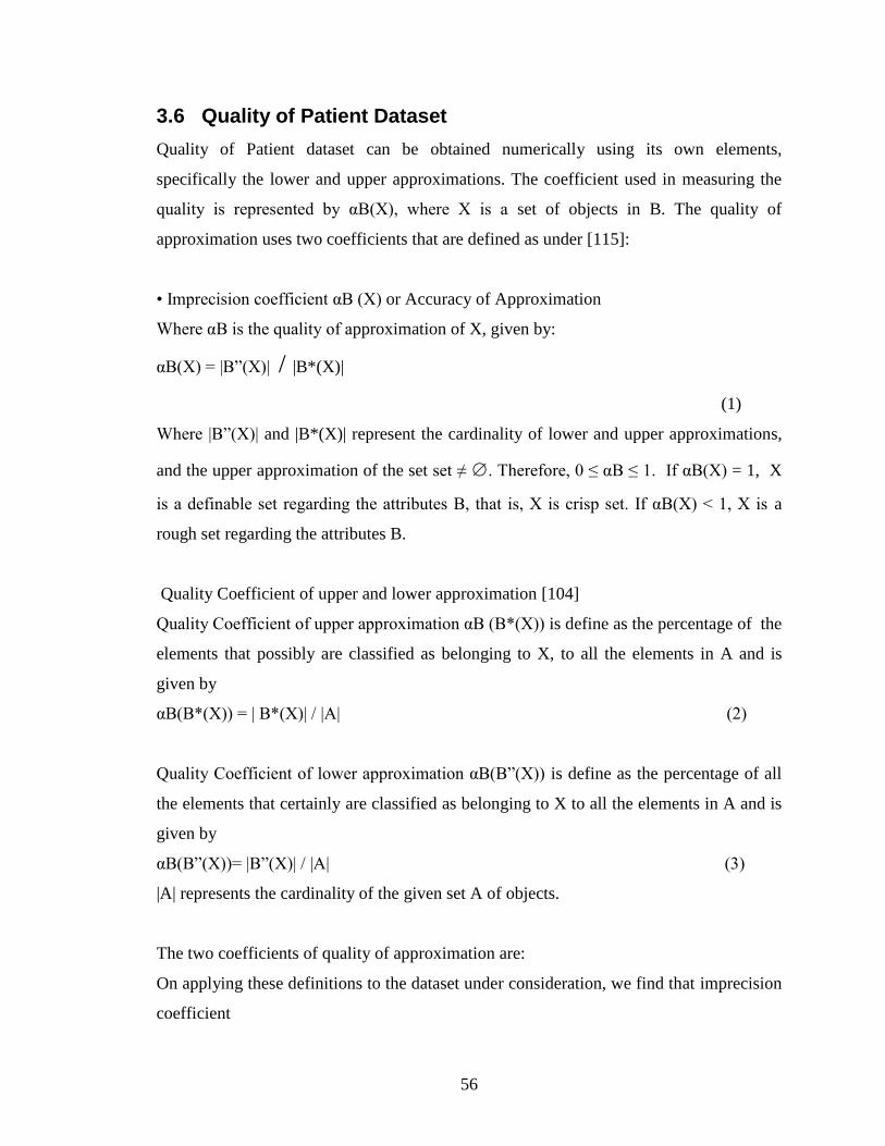
3.6 Quality of Patient Dataset
Quality of Patient dataset can be obtained numerically using its own elements,
specifically the lower and upper approximations. The coefficient used in measuring the
quality is represented by αB(X), where X is a set of objects in B. The quality of
approximation uses two coefficients that are defined as under [115]:
• Imprecision coefficient αB (X) or Accuracy of Approximation
Where αB is the quality of approximation of X, given by:
αB(X) = |B”(X)| / |B*(X)|
(1)
Where |B”(X)| and |B*(X)| represent the cardinality of lower and upper approximations,
and the upper approximation of the set set ≠ ∅. Therefore, 0 ≤ αB ≤ 1. If αB(X) = 1, X
is a definable set regarding the attributes B, that is, X is crisp set. If αB(X) < 1, X is a
rough set regarding the attributes B.
Quality Coefficient of upper and lower approximation [104]
Quality Coefficient of upper approximation αB (B*(X)) is define as the percentage of the
elements that possibly are classified as belonging to X, to all the elements in A and is
given by
αB(B*(X)) = | B*(X)| / |A| (2)
Quality Coefficient of lower approximation αB(B”(X)) is define as the percentage of all
the elements that certainly are classified as belonging to X to all the elements in A and is
given by
αB(B”(X))= |B”(X)| / |A| (3)
|A| represents the cardinality of the given set A of objects.
The two coefficients of quality of approximation are:
On applying these definitions to the dataset under consideration, we find that imprecision
coefficient

57
• For the patients with possibility of Heart Problem αB(X) = 8/10 = 0.80.
• For the patients with possibility of no Heart Problem αB(X) = 5/7 = 0.71.
Quality Coefficient of upper and lower approximation, using Eq. 2 and 3:
• αB(B*(X)) = 10/15, for the patients that have the possibility of Heart Problem.
• αB(B*(X)) = 7/15, for the patients that have the possibility of no Heart Problem.
• αB(B”(X)) = 8/15, for the patients that certainly have Heart Problem.
• αB(B”(X)) = 5/15, for the patients that certainly do not have Heart Problem.
Observations:
1. Patients certainly with heart problem: αB(B”(X)) = 8/15, that is, 53% of patients
certainly have Heart problem.
2. Patients that certainly do not have heart problem: αB(B”(X)) = 5/15, that is,
approximately 33% of patients certainly don't have heart problem.
3. Patients possibly with heart problem: αB(B*(X)) = 10/15, that is, approximately 66%
of patients have the possibility of heart problem.
4. Patients that possibly do not have heart problem: αB(B*(X)) = 7/15, that is, 46% of
the patients do not have the possibility of heart problem.
5. 13% of patients (P8 and P9) cannot be classified as either with heart problem or with
no heart problem.
3.7 Dependency of Patient Dataset
For the analysis of data, it is always important to discover the dependencies between
various attributes. In rough set data analysis also, it is important to discover dependencies
between condition and decision attributes. Intuitively, the set of decision attributes D
depends totally on a set of condition attributes C, and is denoted by C D, provided all
values of attributes of D are uniquely determined by values of attributes of C. In other
words, D depends totally on C, provided there exists a functional dependency between
values of D and C. Formally dependency can be defined in the following way. Let D and
C be the subsets of A. We will say that D depends on C with a degree k (0 k 1),
denoted as C kD, where k = (C, D) [131] (refer to 3.2.12 page 39).

58
γ(C,D) = |POSc(D)| / |U|
In patient dataset we have 8 elements in lower approximation for patients that have heart
problem and 5 elements in lower approximation for patients that do not have heart
problem and the total element in lower approximation is 13 then the dependency
coefficient is calculated as
γ(C,D) = 13/15 = 0.86
So D depends partially (with a degree k=0.86) on C.
3.8 Reduction of Attributes of Patient Dataset
For many applications, it is often necessary to maintain a concise form of the information
system. In every dataset there exists data that can be ignored, without altering the basic
properties and more importantly the consistency of the system. The form in which the
data is presented within an information system should make sure that the redundancy is
avoided as it implicates the minimization of computational complexity in relation to the
creation of rules to extract knowledge. After removing some of the attributes from the
given dataset, if the resultant data set is equivalent to the original dataset in relation to
approximation and dependency, it will be considered as a reduct, since it has the same
approximation precision and same dependency degree as that of the original set of
attributes, however with one fundamental difference, the set of attributes to be considered
will be fewer [104].
The process of reducing an information system such that the set of attributes of the
reduced information system is independent and if no further elimination of attribute can
be done without loosing some information from the system, and then the resultant is
known as a reduct. If an attribute from the subset B A preserves the indiscernibility
relation RA, then the attributes A - B are dispensable. Reducts are such minimal subsets
that do not contain any dispensable attributes. Therefore, the reduct should have the
capacity to classify objects, without altering the form of representation of knowledge.
When the above definition is applied to the information system presented in the table 3.1,
B is a subset of A and the attribute ‘a’ belongs to B such that
• The attribute ‘a’ is dispensable in B if I (B) = I (B - {a}); otherwise ‘a’ is indispensable
attribute in B;

59
• Set B is independent if all of its attributes are indispensable;
• A subset B' of B is a reduct of B if B' is independent and I (B') = I (B);
So a reduct is a set of attributes that preserves the basic characteristics of the original data
set, and the attributes that do not belong to the reduct are superfluous with regard to
classification of elements of the universe.
For finding the reduct of table 3.1 first of all remove inconsistent or inconclusive data
from table 3.1. Data is called inconsistent or inconclusive when all the condition
attributes values are same but they lead to different decision. For patient8 and patient9 in
table 3.1, all the condition attribute values are the same but decision attribute value is
different for them. For patient8 decision value is ‘Yes’ whereas for patient9 decision
value is ‘No’.
After removing Patient8 and Patient9 from Table 3.1 only the consistent part of table is
left as given in table 3.11.
Finding all the reducts in the table is NP Hard problem. Since there can be 2n
-1 reducts
of the dataset where n is the number of attributes. For the above table there may be 127
reducts since there are seven attributes in the dataset. Some of the reducts of table 3.11
have been found as under by using Rose2 software [123]. We have three reduct sets for
patient information system as shown in table 3.12.

60
Patient H.P. B.P. C.P. Cholesterol FT S.O.B R.W.G Heart
Problem
Decision
P1 High High High Normal Low Low High Yes
P2 Low Low High Normal Low Normal Low No
P3 Low High Low Low Normal Low Low No
P4 V_high Low V_high Low Low Normal High Yes
P5 High High V_high Low Low Low High Yes
P6 Low High Low High Low Normal Low No
P7 High High V_high Low Low Low High Yes
P10 V_high Low V_high Low Low Normal High Yes
P11 V_high High High Low Normal Normal High Yes
P12 V_high Low High Low Low Low High Yes
P13 High Low Low Low High Low Low No
P14 Low Low High High Low High Low No
P15 High V_high V_high Normal Low Normal High Yes
Table 3.11 Consistent Part of Patient Dataset
No Reduct Sets
1 {Blood Pressure, Chest Pain, Shortness of Breath, Cholesterol}
2 {Heart Palpitation, Chest Pain, Cholesterol}
3 {Blood Pressure, Chest Pain, Fatigue, Cholesterol}
Table 3.12 Multiple Reducts for the Patient Data Set
For example, a reduct can be a set of condition attributes containing {Blood Pressure,
Chest Pain, Shortness of Breath, Cholesterol} of a patient. With this reduct, the entire 15

61
patient can be correctly classified completely (according to their Heart Problem). A
subset of {Blood Pressure, Chest Pain} is not a reduct of this patient data, because with
only these two attributes one cannot fully classify all the patients of the data set. In
addition, there exists redundancy and contradictions. For example, in table 3.11, with a
subset of {Blood Pressure, Chest Pain}, we cannot correctly classify patient12 and
patient14 as they both have the same values for Blood Pressure and Chest Pain attribute
but different values for Heart Problem decision attribute that is they have different
decisions.
A reduct is often used in the attribute selection process to reduce the number of attributes
by eliminating superfluous attributes towards decision making. We can generate rules
using any of the reducts of table 3.12, for example a patient with Blood Pressure = High
and Chest Pain = High and with Shortness of Breath = Low and Cholesterol = High will
have heart problem. Core attributes form the essential information in a data set and are
contained in all the reducts. From table 3.12, we can see the intersection of all the reducts
is as follows.
Core = {Chest pain, Cholesterol}
Hence Chest Pain and Cholesterol represents the indispensable attributes of the patient
dataset. We can’t remove any of these condition attributes from patient dataset because it
adversely affects our classification.
3.8 Reduct Based Rule Generation
An association rule [6] is a rule of the form α → β, where α and β represent item sets
which do not share common items. The association rule α → β holds in the transaction set
D with confidence c if c% of transactions in D that contain α also contain β. Confidence
can be represented as c = αUβ ⁄α. The rule α → β has support s in the transaction set D if
s% of transactions in D contains α U β. Support can be represented as s = αUβ / D. Here,
we call α antecedent, and β consequent. Confidence gives a ratio of the number of
transactions that the antecedent and the consequent appear together to the number of
transactions the antecedent appears. Support measures how often the antecedent and the
consequent appear together in the transaction set. [137].

62
A decision rule is always in the form of φ→ψ, read as if φ then ψ where φ contains the
condition attributes and ψ contains the decision attributes. Φ and ψ are considered as
condition and decision attributes. We can generate rules from any of the reduct from the
reduct set represented in table 3.12; since the reduct set are the true representations of the
whole dataset. We choose reduct2 of the reduct set i.e. {Heart Palpitation, Chest Pain,
Cholesterol} for generating reduct rules. The rules generated by reduct set are
comparatively lesser in number and are the true representative of the domain. The rules
generated by reduct are called ‘Reduct Rules’ and decision based on these rules are
generally more precise and accurate.
Patient H.P. C.P. Cho Heart
Problem
Decision
P1 High High High Yes
P2 Low High Low No
P3 Low Low Low No
P4 V_high V_high High Yes
P5 High V_high High Yes
P6 Low Low Low No
P7 High V_high High Yes
P10 V_high V_high High Yes
P11 V_high High High Yes
P12 V_high High High Yes
P13 High Low Low No
P14 Low High Low No
P15 High V_high High Yes
Table 3.13 Reduct of Patient Dataset

63
The first step towards the ‘Reduct Rule’ generation is removal of redundancy. For rule
generation the emphasis is on the reduction of the table 3.13 by removing the duplicate
rows, because duplicate rows or cases do not add to any information. The cases which
have equivalent information for all the condition and decision attributes are called
duplicate rows. For patient P3 and P6 in table 3.13 all the decision and condition
attribute values are the same. We can eliminate any one of the patient P3 or P6 from table
3.13. Similarly for patient P5 and P7 all the condition and decision attribute values are
the same. So, we can remove patient P7 from the table further the values of condition and
decision attribute for patient P4 and P10 are the same. So P10 can be eliminated from
table 3.13. Likewise P11 and P12, P2 and P14, P5 and P15 are also same as per their
condition and decision attribute values. So eliminating P6, P7, P10, P12, P14 and P15
from table 3.13 we are left with table 3.14.
Patient H.P. C.P. Cho Heart
Problem
Decision
P1 High High High Yes
P2 Low High Low No
P3 Low Low Low No
P4 V_high V_high High Yes
P5 High V_high High Yes
P11 V_high High High Yes
P13 High Low Low No
Table 3.14 Reduced Table
Rearranging table 3.14 according to Decision attribute values, we get table 3.15.

64
Patient H.P. C.P. Cho Heart
Problem
Decision
P1 High High High Yes
P4 V_high V_high High Yes
P5 High V_high High Yes
P11 V_high High High Yes
P2 Low High Low No
P3 Low Low Low No
P13 High Low Low No
Table 3.15 Rearranging the Reduced Table as per Decision Values
The next step towards the removal of redundancy or reduction is to analyze each
condition attribute one by one independently with decision attribute. Considering the
condition attribute Heart Palpitation with decision attribute i.e. Heart Problem of table
3.13.
Patient H.P. Heart
Problem
Decision
P1 High Yes
P4 V_high Yes
P5 High Yes
P11 V_high Yes
P2 Low No
P3 Low No
P13 High No
Table 3.16 Heart Palpitation with Decision

65
Further reduction in table 3.16 is possible because the values of condition and decision
attributes for patients P1 and P5 are the same. Likewise P4 and P11, P2 and P3 are same.
Removing P3, P5 and P11 from the table 3.16 result is table 3.17.
Patient H.P. Heart
Problem
Decision
P1 High Yes
P4 V_high Yes
P2 Low No
P13 High No
Table 3.17 Reduced Heart Palpitation with Decision
Now considering the condition attribute Chest Pain with decision attribute Heart Problem
and removing duplicate cases that is P5, P11 and P13 a new table 3.18 is formed.
Patient C.P. Heart
Problem
Decision
P1 High Yes
P4 V_high Yes
P2 High No
P3 Low No
Table 3.18 Reduced Chest Pain with Decision
Similarly considering the condition attribute Cholesterol with decision attribute Heart
Problem and removing the duplicate rows of P3, P4, P5 and P11, P13 we are left with the
table 3.19.

66
Patient Cho Heart
Problem
Decision
P1 High Yes
P2 Low No
Table 3.19 Reduced Cholesterol with Decision
In the next step taking the intersection (Verification of equivalent) of data records in
tables 3.17, 3.18 and 3.19 and joining the data values for various attributes, we get table
3.20, where data records is the element of reduct information in relation to Table 3.1.
Patient H.P. C.P. Cho Heart
Problem
Decision
P1 High High High Yes
P2 Low High Low No
Table 3.20 Joining of Information
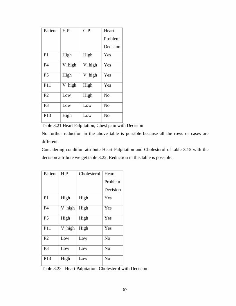
The next step of the analysis is to consider the condition attributes in pairs with decision
attribute and then eliminating the duplicate rows. Considering condition attributes Heart
Palpitation and Chest Pain of table 3.15 with decision attribute Heart Problem and
analyzing the table.
67
Patient H.P. C.P. Heart
Problem
Decision
P1 High High Yes
P4 V_high V_high Yes
P5 High V_high Yes
P11 V_high High Yes
P2 Low High No
P3 Low Low No
P13 High Low No
Table 3.21 Heart Palpitation, Chest pain with Decision
No further reduction in the above table is possible because all the rows or cases are
different.
Considering condition attribute Heart Palpitation and Cholesterol of table 3.15 with the
decision attribute we get table 3.22. Reduction in this table is possible.
Patient H.P. Cholesterol Heart
Problem
Decision
P1 High High Yes
P4 V_high High Yes
P5 High High Yes
P11 V_high High Yes
P2 Low Low No
P3 Low Low No
P13 High Low No
Table 3.22 Heart Palpitation, Cholesterol with Decision

68
After removing duplicate cases of P3, P5 and P11 from table 3.22, a new table 3.23 is
formed.
Patient H.P. Cho Heart
Problem
Decision
P1 High High Yes
P4 V_high High Yes
P2 Low Low No
P13 High Low No
Table 3.23 Reduced Heart Palpitation, Cholesterol with Decision
Considering condition attributes Chest Pain and Cholesterol with decision attribute Heart
Problem of table 3.15 and getting table 3.24.
Patient C.P. Cho Heart
Problem
Decision
P1 High High Yes
P4 V_high High Yes
P5 V_high High Yes
P11 High High Yes
P2 High Low No
P3 Low Low No
P13 Low Low No
Table 3.24 Chest Pain, Cholesterol with Decision

69
In the above table there are three duplicate cases i.e. P5, P11 and P13. Removing the
redundancy from the above table we are left with the following table 3.25.
Patient C.P. Cho Heart
Problem
Decision
P1 High High Yes
P4 V_high High Yes
P2 High Low No
P3 Low Low No
Table 3.25 Reduced Chest Pain, Cholesterol with Decision
Taking the intersection of the records in reduced tables 3.21, 3.23 and 3.25 will lead us to
the table 3.26.
Patient H.P. C.P. Cho Heart
Problem
Decision
P1 High High High Yes
P4 V_high V_high High Yes
P2 Low High Low No
Table 3.26 Join of Information
In the next step taking the intersection of records in table 3.20 and table 3.26 we get the
table 3.27 that provides the minimum number of significant rules.

70
Patient H.P. C.P. Cho Heart
Problem
Decision
P1 High High High Yes
P2 Low High Low No
Table 3.27 Rule Generation Table
Decision rules are often presented as implications and are called ”if... then...” rules. A set
of decision rules is called a decision algorithm. Thus with each decision table we can
associate a decision algorithm consisting of all decision rules occurring in the decision
tables. We must however, make distinction between decision tables and decision
algorithms. A decision table is a collection of data, whereas a decision algorithm is a
collection of implications, or logical expressions. To deal with data we use various
mathematical methods, such as statistics [78], but to analyze implications we must
employ logical tools [103]. Thus these two approaches are not equivalent; however for
simplicity we will often present here decision rules in form of implications, without
referring deeper to their logical nature, as it is often practiced in AI.
Decision Rules according to table 3.27 are
Rule 1
If (Heart Palpitation = High) and (Chest Pain = High) and (Cholesterol = High)
Then Heart Problem = Yes
Rule 2
If (Heart Palpitation = Low) and (Chest Pain = High) and (Cholesterol = low)
Then Heart Problem = No
These rules are most significant rules and are the true representative of the patient dataset.
These rules are sufficient to define the patient dataset.

71
Rules generated by Rose2 [123] software for patient dataset is shown in fig. 3.2.
Fig. 3.2 Rules Generated by Rose2 Software for Patient Dataset
The number of rules generated by our method is less than the rules generated by Rose2
software. In this chapter we have demonstrated the use of Rough Set Theory for the
generation of rules with minimum number of condition attributes that provides the sound
inference. The rule set may not be complete as it may not define the decision for certain
sets of values for the attributes.

72
But the aim here is to find the minimum number of rules that could be the representative
of knowledge provided by the dataset, and must be sound in nature as per AI
nomenclature. The rules generated by reduct based method are validated. These rules
proved to be sound in nature.
The numbers of rules generated by the proposed method are relatively less in number as
compared to the rules generated by the Rose2 software available in literature.