Embed Size (px)
Citation preview
101
CHAPTER 4
STUDY AREA DESCRIPTION AND
DATABASE GENERATION
4.1 DESCRIPTION OF THE STUDY AREA
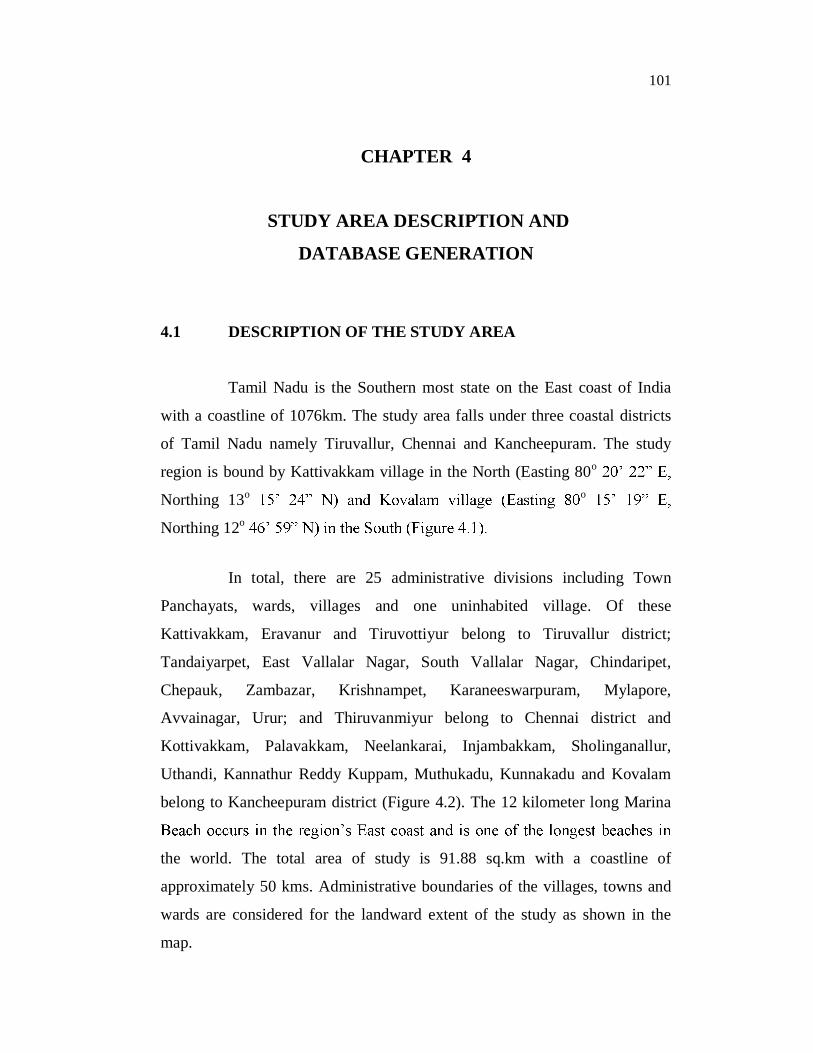
Tamil Nadu is the Southern most state on the East coast of India
with a coastline of 1076km. The study area falls under three coastal districts
of Tamil Nadu namely Tiruvallur, Chennai and Kancheepuram. The study
region is bound by Kattivakkam village in the North (Easting 80o
Northing 13o o
Northing 12o
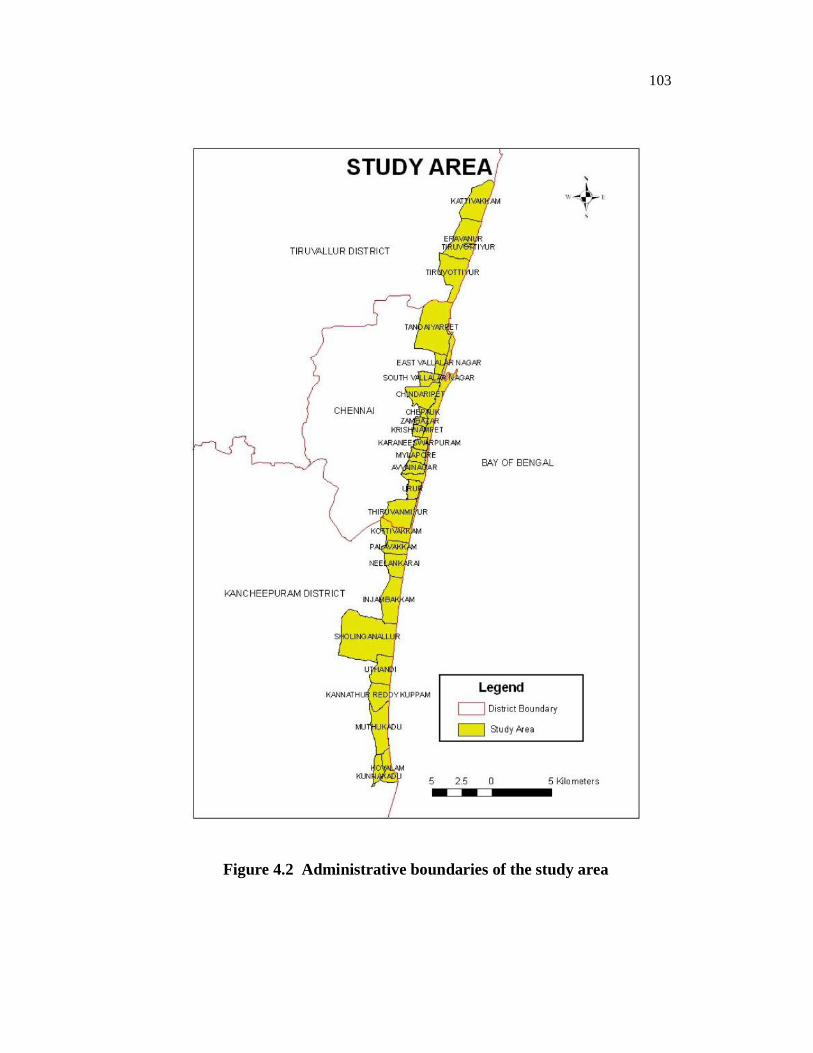
In total, there are 25 administrative divisions including Town
Panchayats, wards, villages and one uninhabited village. Of these
Kattivakkam, Eravanur and Tiruvottiyur belong to Tiruvallur district;
Tandaiyarpet, East Vallalar Nagar, South Vallalar Nagar, Chindaripet,
Chepauk, Zambazar, Krishnampet, Karaneeswarpuram, Mylapore,
Avvainagar, Urur; and Thiruvanmiyur belong to Chennai district and
Kottivakkam, Palavakkam, Neelankarai, Injambakkam, Sholinganallur,
Uthandi, Kannathur Reddy Kuppam, Muthukadu, Kunnakadu and Kovalam
belong to Kancheepuram district (Figure 4.2). The 12 kilometer long Marina
the world. The total area of study is 91.88 sq.km with a coastline of
approximately 50 kms. Administrative boundaries of the villages, towns and
wards are considered for the landward extent of the study as shown in the
map.
102
India Tamil Nadu
Study Region
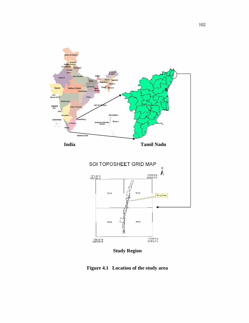
Figure 4.1 Location of the study area
103
Figure 4.2 Administrative boundaries of the study area
104
The entire study area is occupied by settlements mainly belonging
to the coastal community. Major industries like fertilizer and rubber factories,
steel rolling industries, and petrochemical companies are located on the
northeast coast of Chennai. Beach resorts, farmhouses, aquaculture ponds,
theme parks, tourist spots, and artificial parks are mainly located on the
southeast coast of Chennai. Fishing is the main occupation of the people
living in the suburban coastline, whereas in the urban coastline, the
occupation is not only fishing but also depends upon urban resources like
industries and government and non-government organisations (Kumar et al
2008).
4.2 DATABASE GENERATION
4.2.1 Data Source and Software
The data related to the study area and hazards have been collected
from various sources and a detailed database has been generated. The data
used in the study comprises of Satellite data, collateral data and attribute data.
The base or reference map has been digitized from Survey of India
topographical sheets numbering 66C04, 66C08, 66D01 AND 66D05,
published in the year 1970-1971, in the scale of 1:50000. Transverse Mercator
projection with WGS 84 datum has been used for the maps.
4.2.2 Satellite data and other data
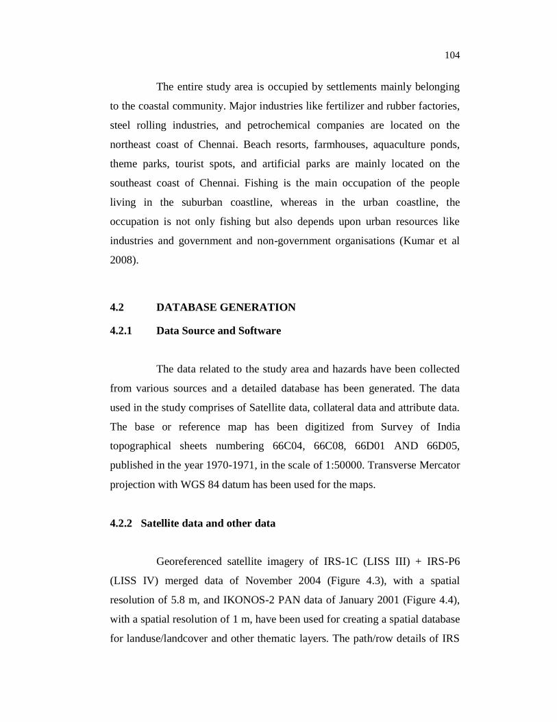
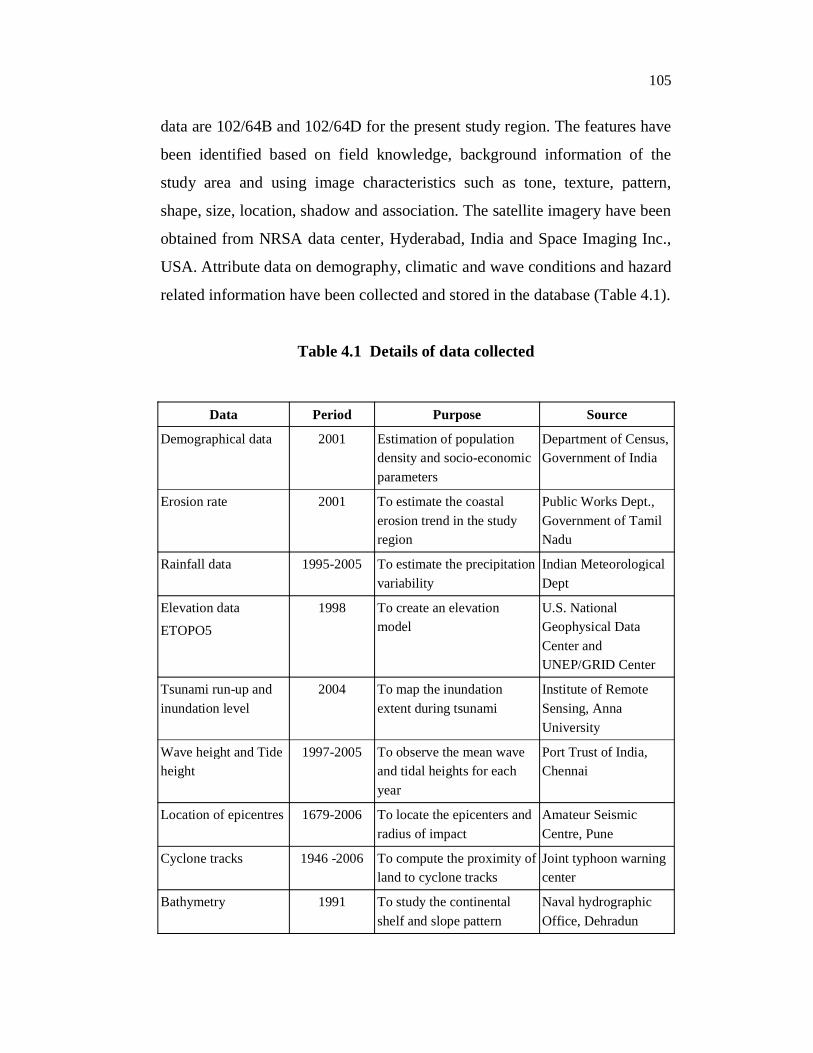
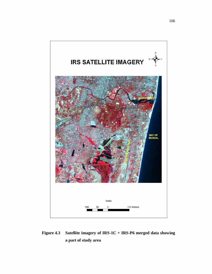
Georeferenced satellite imagery of IRS-1C (LISS III) + IRS-P6
(LISS IV) merged data of November 2004 (Figure 4.3), with a spatial
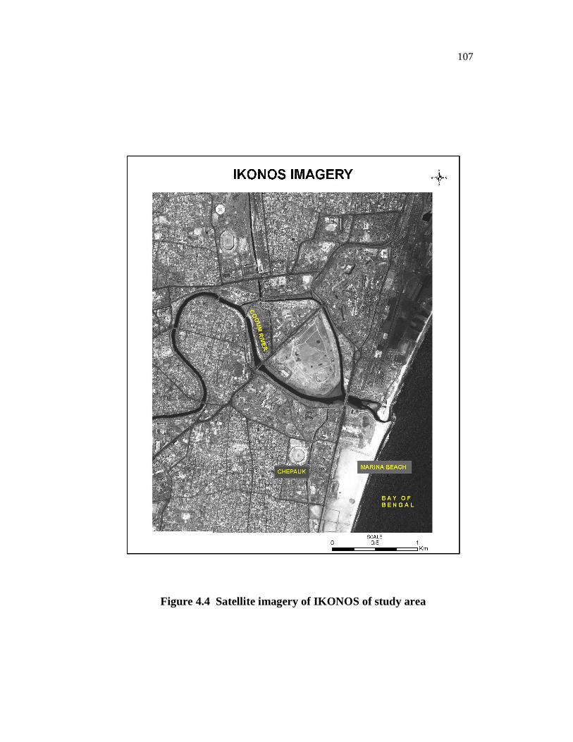
resolution of 5.8 m, and IKONOS-2 PAN data of January 2001 (Figure 4.4),
with a spatial resolution of 1 m, have been used for creating a spatial database
for landuse/landcover and other thematic layers. The path/row details of IRS
105
data are 102/64B and 102/64D for the present study region. The features have
been identified based on field knowledge, background information of the
study area and using image characteristics such as tone, texture, pattern,
shape, size, location, shadow and association. The satellite imagery have been
obtained from NRSA data center, Hyderabad, India and Space Imaging Inc.,
USA. Attribute data on demography, climatic and wave conditions and hazard
related information have been collected and stored in the database (Table 4.1).
Table 4.1 Details of data collected
Data Period Purpose Source
Demographical data 2001 Estimation of population density and socio-economic parameters
Department of Census, Government of India
Erosion rate 2001 To estimate the coastal erosion trend in the study region
Public Works Dept., Government of Tamil Nadu
Rainfall data 1995-2005 To estimate the precipitation variability
Indian Meteorological Dept
Elevation data
ETOPO5
1998 To create an elevation model
U.S. National Geophysical Data Center and UNEP/GRID Center
Tsunami run-up and inundation level
2004 To map the inundation extent during tsunami
Institute of Remote Sensing, Anna University
Wave height and Tide height
1997-2005 To observe the mean wave and tidal heights for each year
Port Trust of India, Chennai
Location of epicentres 1679-2006 To locate the epicenters and radius of impact
Amateur Seismic Centre, Pune
Cyclone tracks 1946 -2006 To compute the proximity of land to cyclone tracks
Joint typhoon warning center
Bathymetry 1991 To study the continental shelf and slope pattern
Naval hydrographic Office, Dehradun
106
Figure 4.3 Satellite imagery of IRS-1C + IRS-P6 merged data showing
a part of study area
107
Figure 4.4 Satellite imagery of IKONOS of study area
108
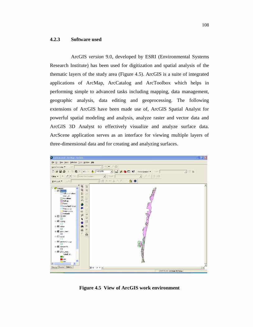
4.2.3 Software used
ArcGIS version 9.0, developed by ESRI (Environmental Systems
Research Institute) has been used for digitization and spatial analysis of the
thematic layers of the study area (Figure 4.5). ArcGIS is a suite of integrated
applications of ArcMap, ArcCatalog and ArcToolbox which helps in
performing simple to advanced tasks including mapping, data management,
geographic analysis, data editing and geoprocessing. The following
extensions of ArcGIS have been made use of, ArcGIS Spatial Analyst for
powerful spatial modeling and analysis, analyze raster and vector data and
ArcGIS 3D Analyst to effectively visualize and analyze surface data.
ArcScene application serves as an interface for viewing multiple layers of
three-dimensional data and for creating and analyzing surfaces.
Figure 4.5 View of ArcGIS work environment
109
ERDAS Imagine version 8.5 (http://www.erdas.com) has been used
to interpret the satellite imagery of the region and derive the various landuse
and geomorphologic categories. Also the topographic features of the study
area have been extracted using this software. The elevation profile has been
analysed using Global Mapper version 6.0 (http://www.globalmapper.com).
The multi-criteria analysis has been performed using Criterium
Decision Plus version 3.0.4 (http://www.infoharvest.com/infoharv/). CDP is a
graphical user interface that generates a decision hierarchy directly from a
brainstorming model which comprises the alternatives and criteria. Graphic
analysis of the results by criteria, weights or sensitivity to changes in weights
are useful in reviewing the results. For statistical analysis and
graphs/maps/charts preparation purposes, Microsoft-Access, Microsoft-Excel
and Microsoft-Word have been used.
4.3 ENVIRONMENTAL SCENARIO
Visual Interpretation based on the tonal characteristics of IRS
satellite imagery, coastal geomorphological and landuse categories have been
demarcated using ERDAS Imagine software and have been plotted on the
base map prepared using the SOI topographical maps on 1:50,000 scale.
Digitization of geocoded IRS 1C (LISS III) + IRS P6 (LISS IV) merged
satellite data have been carried out for deriving the primary dataset of various
themes. The classification scheme follows the NRIS (National- Natural
Resources Information System) standard developed by the Department of
Space (NRIS 1997). Other collateral information like tidal data, wave data
etc. have been collected through secondary sources. These data have been
integrated in spatial framework in GIS environment for analysis.
110
4.3.1 Geomorphology
The satellite imagery has been visually interpreted into geomorphic
units/ landforms based on image elements such as tone, texture, shape, size,
location and association, physiography, genesis of landforms, nature of rocks/
sediments, and associated geological structures. The topographic information
in SOI toposheets has been helpful in interpreting the satellite imagery. Major
geomorphic units have been mapped based on physiography and relief.
Within each zone different geomorphic units have been mapped based on
landform characteristics, their areal extent, depth of weathering and thickness
of deposition (Table 4.2). The features have been labeled as per the NRIS
(National-Natural Resources Information System) coding scheme and linked
to the Look-Up-Table (LUT) (NRIS 1997). The coverage has been projected
and transformed into Transverse Mercator projection and coordinate system
in meters. The transformation process involves geometric rectification
through Ground Control Points (GCPs) identified on the input coverage and
corresponding SOI map.
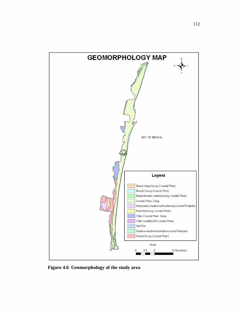
Geomorphologically, the study area comprises younger and older
coastal alluvial plains. The younger coastal plain is characterised by narrow to
wider beaches followed by beach sand ridges, which are gently sloping
towards sea side and swale complexes of swamps/ marshes, mud flat and salt
flats. The area is a vast coastal plain characterized by several strandlines,
lagoon , mangroves, salt marsh, estuaries, creek , barred dunes, spits and
beach terraces (Figure 4.6). The salt flats are utilized as saltpans around
Muthukadu.
The Beach runs continuously all along the study area from
Kattivakkam to Kovalam river mouth, except where coastal inlets/creeks are
present. There are several stabilized sand dunes with vegetation growth.
111
Towards onshore, the East Coast road has dissected the dunes. Berms are
present almost in the entire study area. At Kovalam, they are present in the
fore shore region where wave action is dominant.
Table 4.2 Geomorphic Classification (NRIS 1997)
Zone Geomorphic Unit Sub-Category
Pediplain Pediplain Weathered/
buried
Shallow weathered/shallow buried
Pediplain
Moderately weathered/moderately
buried Pediplain
Coastal
Plain
Old Coastal Plain Older mudflat(Old Coastal Plain)
Older Coastal Plain Deep
Young Coastal Plain
Beach ridge(Young Coastal Plain)
Swale(Young Coastal Plain)
Brackishwater creeks
Coastal Plain Deep
Mud flat(Young Coastal Plain)
Beach(Young Coastal Plain)
Salt Pan
There are seawater inlets/creeks present in the study area, namely
Ennore creek, and Muthukadu creek that is present north of Kovalam.
Buckingham canal runs parallel to shore throughout the length of the region.
The Coastal wetlands run west of the Buckingham canal. Also, tidal flats are
spread around the Buckingham Canal. The shoreline is appreciably straight,
open and continuous. The beaches vary in width from 35 metres to 1000
metres and beaches of about 50 m in width are very common and show
normally well developed foredunes and backshore berms. The foreshore has a
gentle slope and the surf zone wide.
112
Figure 4.6 Geomorphology of the study area
113
Small rocky outcrops, close to the seawater front exist at Kovalam
beach of Kovalam creek. The rocky outcrops are garnetiferous charnockite/
granitic gneiss with coarse to medium grained granitic texture. Rock
cleavages and slip planes are seen along biotite enriched portions. At the mid
point of the bay, rocky exposures occur in the foreshore region, which are
weathered due to wave action.
Beyond the berm region, acidic charnockite is present. In the wave
cut terrace, sandy layers of heavy mineral bands are formed. Towards the
mouth of Muthukadu creek, all along the foreshore and berm, heavy mineral
concentrations occur. The entire coastline exhibits bundles of beach ridges
which act as potential zones of ground water.
4.3.2 Geology
Classification and mapping of lithologic units/rock types is
performed through visual interpretation of image characteristics and terrain
information, supported by the a priori knowledge of general geologic setting
of the area. The tone (colour) and landform characteristics, and relative
erodibility, drainage, soil type, land use/cover and other contextual
information are used in classification. The rock types are mapped and labeled
as per NRIS classification scheme (Table 4.3) (NRIS 1997).
The geology of the study area comprises of mostly clay, shale and
sandstone. The Chennai city is classified into three regions based on geology:
sandy areas, clayey areas and hard-rock areas. Sandy areas are found along
the river banks and coasts. Igneous/metamorphic rocks are found in the south
of Chennai; marine sediments containing clay-silt sands and charnockite
rocks are found in the eastern and northern parts; and the western parts are
composed of alluvium and sedimentary rocks.
114
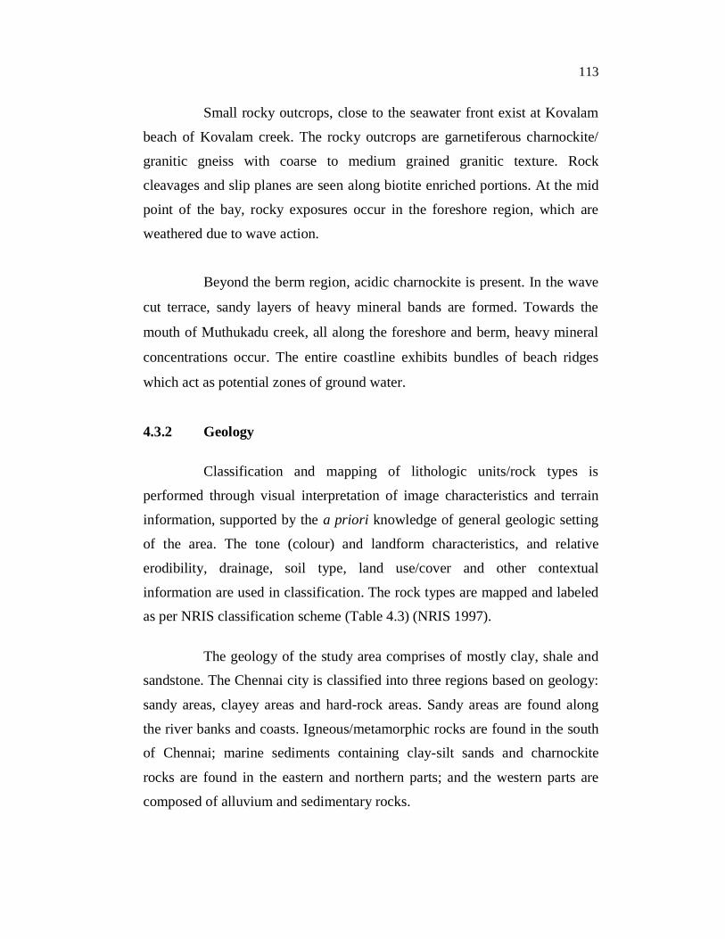
Clayey regions cover most of the city. The thickness of soil
formation ranges from a few meters in the southern part to as much as 50
meters in the northern and central parts (Figure 4.7). The geological
formations are beach sands at Quaternary and recent periods. Cuddalore
sandstone of Mio- Pliocene age, shoals and sand stone of upper Gondwanas
and Chornockites of Archaean era also occur.
Table 4.3 Lithologic Unit Classification (NRIS 1997)
Lithologic Unit Rock Type Stratigraphy
Clay Fluvial-Flood basin deposits Quaternary
Clayey sand Fluvio-Marine Quaternary
Sand, Silt and
Clay Partings
Alluvium-Fluvial Quaternary
Sand and silt Alluvium- Fluvial Quaternary
Sandstone Cuddalore Formation Mio-pliocene\Cainozoic
Charnockite Charnockite Group Archaean
The coastal zone between Kattivakkam and Kovalam is basically
comprised of recent coastal Alluvium, with a mixture of fine-grained light
white sands with broken shell pieces. The alluvium consists of sand, silt and
clay. The thickness of alluvium varies from 10 m to 28 m with a maximum observed of 9.6 m.
The presence of thick black clay followed by fossil bed below
alluvium is a common feature. Fluvial marine and erosional landforms have
been found. The coastal sands lie over the Charnockite basement with an
average depth ranging from 12- 20m and intercalated with occasional reddish brown clays.
115
Figure 4.7 Geology of the study area
116
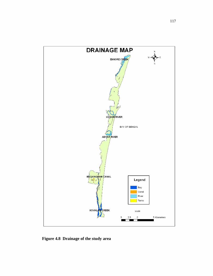
4.3.3 Drainage and Hydrology
The classification covers perennial, seasonal and peripheral
categories (NRIS 1997). Minor streams and rivers have been represented by
line, while the major rivers with edges in the SOI map have been represented
by polygons. Two rivers meander through the study region, the Cooum (or
Koovam) in the central region and the Adyar in the southern region.
A protected estuary of the Adyar forms the natural habitat of
several species of birds and animals. These two rivers are almost stagnant and
do not carry enough water except during rainy seasons. The Buckingham
Canal travels parallel to the coast, linking the two rivers. The Otteri Nullah,
an east-west stream runs through north Chennai and meets the Buckingham
Canal at Basin Bridge (Figure 4.8).
The Chennai city is served by two major ports namely the Chennai
Port which is one of the largest artificial ports and the Ennore Port. A smaller
harbour at Royapuram is used by local fishing boats and trawlers. Numerous
perennial and dry tanks are spread over the study region.
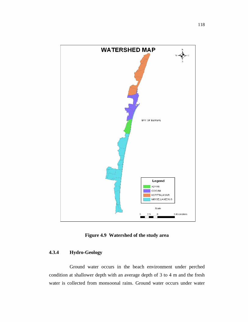
The primary layers of hydrologic units upto watershed have been
created (Figure 4.9). The classification scheme follows the hierarchical
system of watershed delineation developed by AISLUS (All India Soil and
Landuse Survey). Each water resources region is delineated into basins and
each basin is subdivided into catchments. Each catchment is divided into
subcatchments and each sub-catchment is divided into watersheds, drained by
a single river or group of small rivers or a tributary of a major river.
117
Figure 4.8 Drainage of the study area
118
Figure 4.9 Watershed of the study area
4.3.4 Hydro-Geology
Ground water occurs in the beach environment under perched
condition at shallower depth with an average depth of 3 to 4 m and the fresh water is collected from monsoonal rains. Ground water occurs under water
119
table conditions, the major water bearing formation being the coastal sands. Groundwater occurs in water table under semi-confined to confined
conditions in the porous alluvial formations. Near the boundary and in the low
lying areas, estuarine deposits and the fluvial action by rivers have deposited
very irregular lenses of sand and silt layers. The important aquifer systems in the Tiruvallur district are constituted by unconsolidated and semi-
consolidated formations, weathered and fractured crystalline rocks. The
general gradient and ground water flow in Kancheepuram district is towards
east. In the creeks, low lying areas, salt pans and along the Buckingham channel, water is always saline due to the sea water incoming into the channel
during high tides.
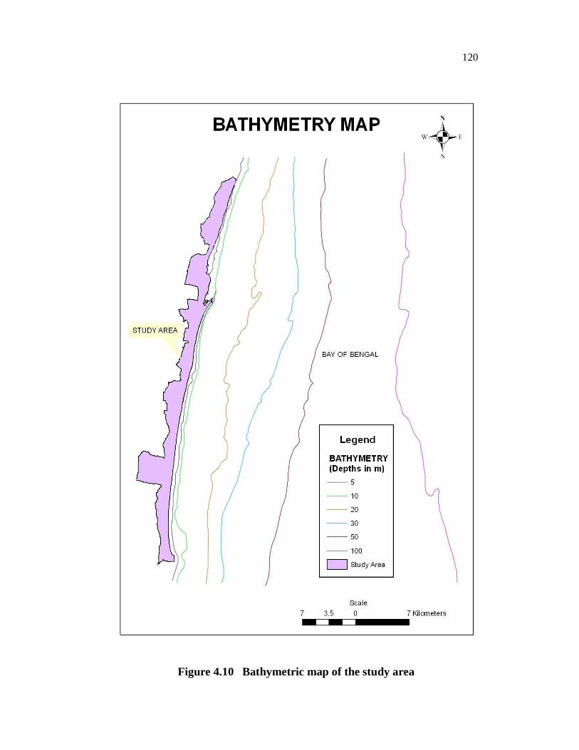
4.3.5 Bathymetry
Bathymetric maps show the depth and slope of the ocean floor near
the shore and are used to assess the potential impacts of storm surges and tides on coastal areas. The bathymetric maps are helpful in knowing the
coastal configuration with respect to depths of the sea. The bathymetry map for the study area has been prepared by digitizing the hydrographic chart of
Mamallapuram to Point Pudi published by the Naval Hydrographic Office,
Dehradun using ArcGIS software. The scale of the map is 1: 150000.
The bathymetric profile of the Eastern continental margin of India
shows that the shelf is in general steep and narrow in the south (except off
Chennai), whereas it is relatively wider and gentle in the north. The coastline
is oriented in N S direction. The width of the continental shelf is 43 km off
Chennai and depth at which shelf-break occurs is 200m at Chennai (Figure
4.10). South of Chennai, the shelf is non-basinal where the inner and middle
shelf is smooth and featureless; outer shelf shows bottom irregularities as
much as to 4 to 6 m, related to karstic structures, pinnacles and smooth dome
shaped reef structures.
120
Figure 4.10 Bathymetric map of the study area
121
Off Chennai the width of the continental slope is narrow (9km) with a steep gradient (250 m/km) (Rao et al 1992) and appears to be devoid of
gullies and valleys (Table 4.2). The shallow bays associated with basinal
areas are more affected by the crossing of cyclones and storm surges, due to
wider shelf with gentle slope.
Table 4.4 Continental Shelf Characteristics of Chennai
Location Water depth
at shelf break m
Shelf edge distance form
coast km
Shelf gradient
Ratio
Slope gradient
Ratio
Depth at which
marginal high is
recorded m
Chennai 200 55 1:200 1:8 2700
4.3.6 Structural Details
Different types of primary and secondary geological structures
(attitude of beds, schistocity / foliation, folds, lineaments, circular features)
could be visually interpreted from imagery by studying the landforms, slope
asymmetry, outcrop pattern, drainage pattern, and stream/ river courses.
Lineaments (faults, fractures, shear zones, and thrusts) appear as linear and
curvilinear lines on the satellite imagery, and are often indicated by the
presence of moisture, alignment of vegetation, straight drainage courses and
alignment of tanks / ponds. Lineaments are further sub-divided based on
image characteristics and geological evidence (NRIS 1997).
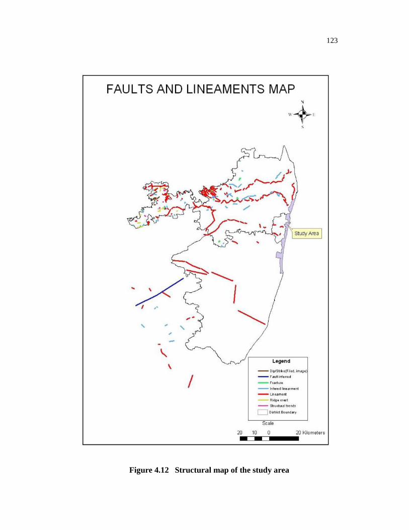
Structural maps, which show the location of the major geological
fault systems and related geological features, are used to identify the loci of
earthquakes and zones of earth movement (Figure 4.11). A NW SE trending
mega lineament occurs from Chennai on the east coast. The structural map for
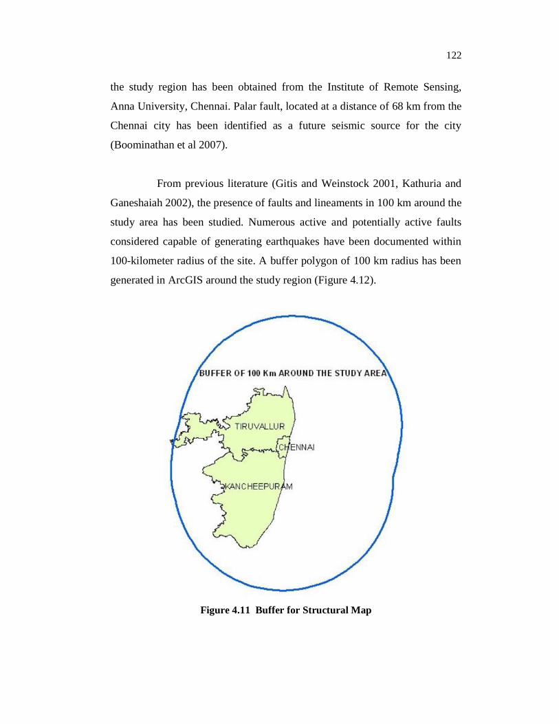
122
the study region has been obtained from the Institute of Remote Sensing,
Anna University, Chennai. Palar fault, located at a distance of 68 km from the
Chennai city has been identified as a future seismic source for the city
(Boominathan et al 2007).
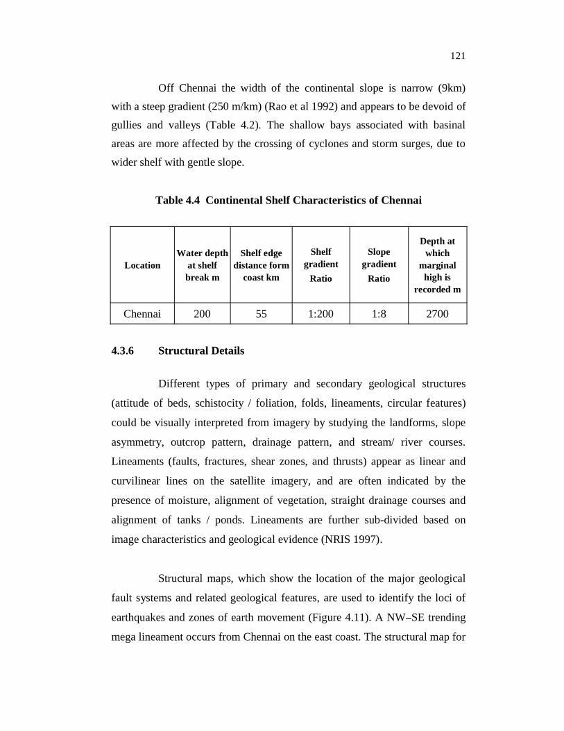
From previous literature (Gitis and Weinstock 2001, Kathuria and
Ganeshaiah 2002), the presence of faults and lineaments in 100 km around the
study area has been studied. Numerous active and potentially active faults
considered capable of generating earthquakes have been documented within
100-kilometer radius of the site. A buffer polygon of 100 km radius has been
generated in ArcGIS around the study region (Figure 4.12).
Figure 4.11 Buffer for Structural Map
123
Figure 4.12 Structural map of the study area
124
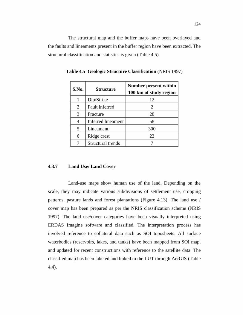
The structural map and the buffer maps have been overlayed and
the faults and lineaments present in the buffer region have been extracted. The
structural classification and statistics is given (Table 4.5).
Table 4.5 Geologic Structure Classification (NRIS 1997)
S.No. Structure Number present within 100 km of study region
1 Dip/Strike 12 2 Fault inferred 2 3 Fracture 28 4 Inferred lineament 58 5 Lineament 300 6 Ridge crest 22 7 Structural trends 7
4.3.7 Land Use/ Land Cover
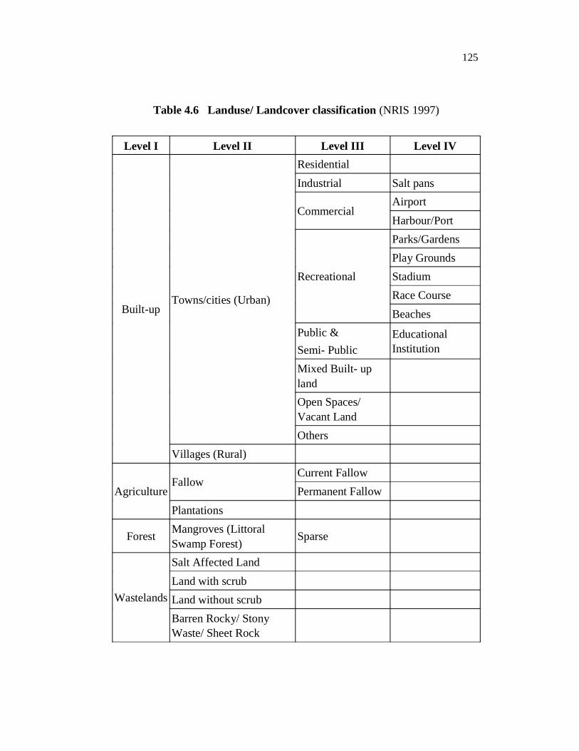
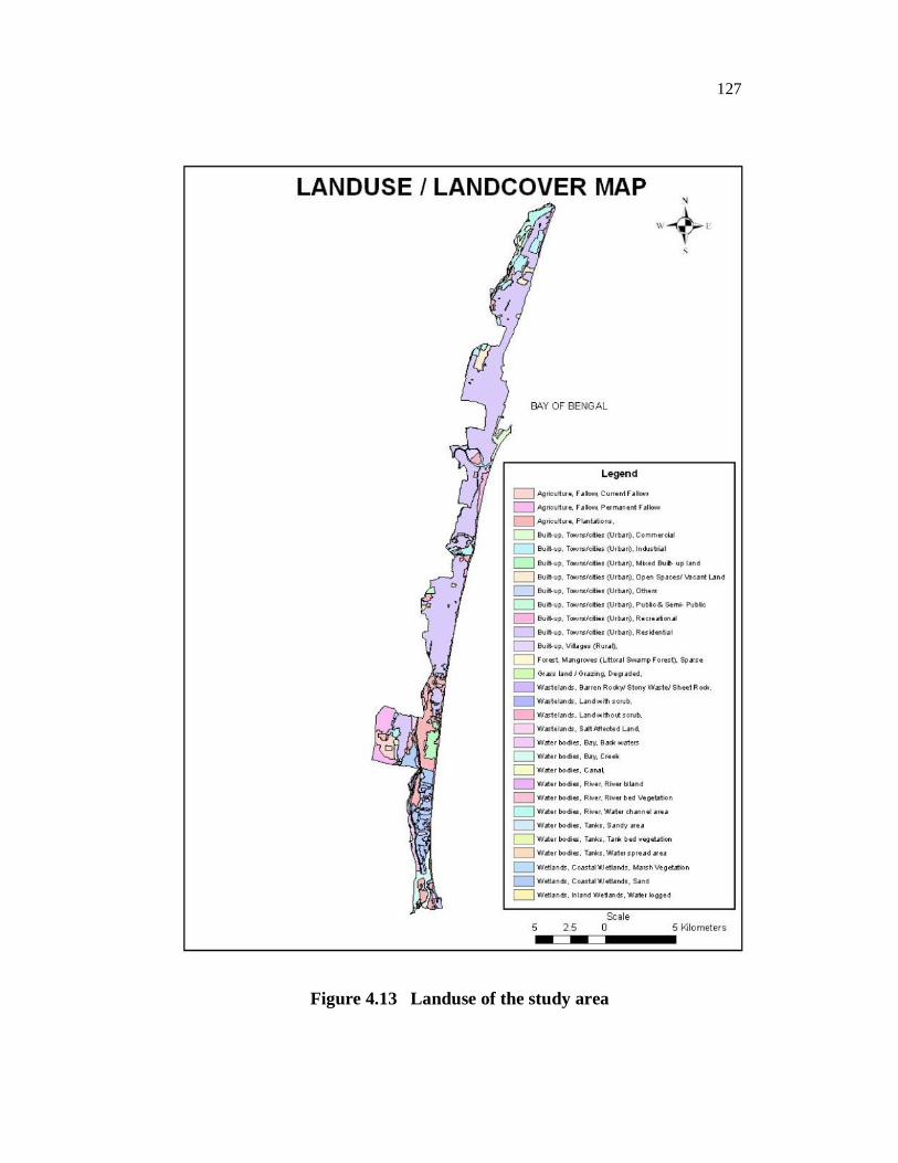
Land-use maps show human use of the land. Depending on the
scale, they may indicate various subdivisions of settlement use, cropping
patterns, pasture lands and forest plantations (Figure 4.13). The land use /
cover map has been prepared as per the NRIS classification scheme (NRIS
1997). The land use/cover categories have been visually interpreted using
ERDAS Imagine software and classified. The interpretation process has
involved reference to collateral data such as SOI toposheets. All surface
waterbodies (reservoirs, lakes, and tanks) have been mapped from SOI map,
and updated for recent constructions with reference to the satellite data. The
classified map has been labeled and linked to the LUT through ArcGIS (Table
4.4).
125
Table 4.6 Landuse/ Landcover classification (NRIS 1997)
Level I Level II Level III Level IV
Built-up Towns/cities (Urban)
Residential Industrial Salt pans
Commercial Airport Harbour/Port
Recreational
Parks/Gardens Play Grounds Stadium Race Course Beaches
Public & Semi- Public
Educational Institution
Mixed Built- up land
Open Spaces/ Vacant Land
Others Villages (Rural)
Agriculture Fallow
Current Fallow Permanent Fallow
Plantations
Forest Mangroves (Littoral Swamp Forest) Sparse
Wastelands
Salt Affected Land Land with scrub Land without scrub Barren Rocky/ Stony Waste/ Sheet Rock
126
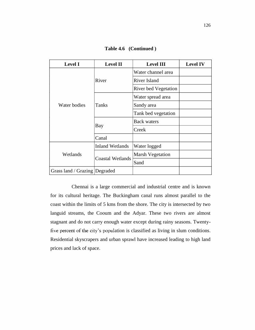
Table 4.6 (Continued )
Level I Level II Level III Level IV
Water bodies
River Water channel area River Island River bed Vegetation
Tanks Water spread area Sandy area Tank bed vegetation
Bay Back waters Creek
Canal
Wetlands Inland Wetlands Water logged
Coastal Wetlands Marsh Vegetation Sand
Grass land / Grazing Degraded
Chennai is a large commercial and industrial centre and is known
for its cultural heritage. The Buckingham canal runs almost parallel to the
coast within the limits of 5 kms from the shore. The city is intersected by two
languid streams, the Cooum and the Adyar. These two rivers are almost
stagnant and do not carry enough water except during rainy seasons. Twenty-
ation is classified as living in slum conditions.
Residential skyscrapers and urban sprawl have increased leading to high land
prices and lack of space.
127
Figure 4.13 Landuse of the study area
128
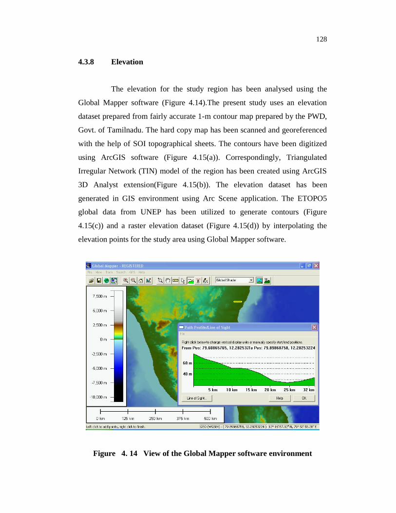
4.3.8 Elevation
The elevation for the study region has been analysed using the
Global Mapper software (Figure 4.14).The present study uses an elevation
dataset prepared from fairly accurate 1-m contour map prepared by the PWD,
Govt. of Tamilnadu. The hard copy map has been scanned and georeferenced
with the help of SOI topographical sheets. The contours have been digitized
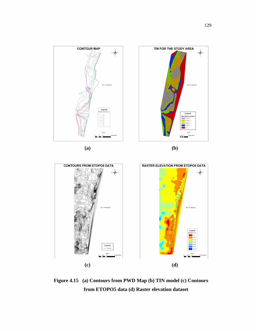
using ArcGIS software (Figure 4.15(a)). Correspondingly, Triangulated
Irregular Network (TIN) model of the region has been created using ArcGIS
3D Analyst extension(Figure 4.15(b)). The elevation dataset has been
generated in GIS environment using Arc Scene application. The ETOPO5
global data from UNEP has been utilized to generate contours (Figure
4.15(c)) and a raster elevation dataset (Figure 4.15(d)) by interpolating the
elevation points for the study area using Global Mapper software.
Figure 4. 14 View of the Global Mapper software environment
129
(a) (b)
(c) (d)
Figure 4.15 (a) Contours from PWD Map (b) TIN model (c) Contours
from ETOPO5 data (d) Raster elevation dataset
130
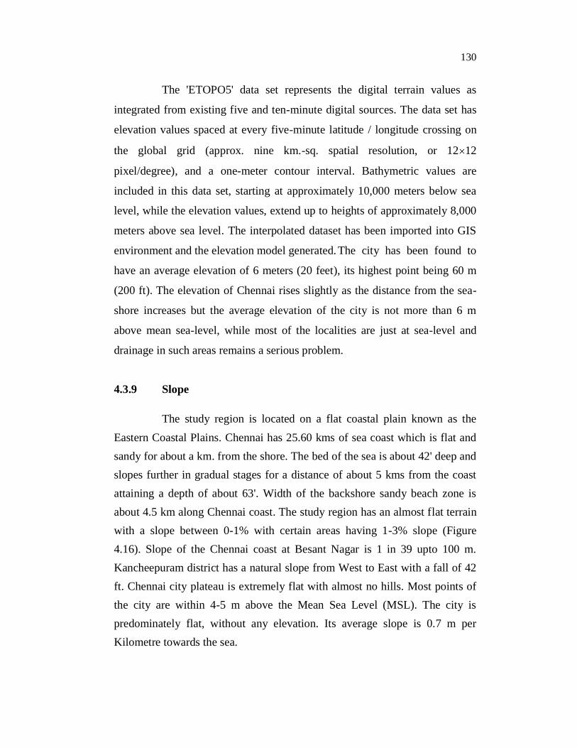
The 'ETOPO5' data set represents the digital terrain values as
integrated from existing five and ten-minute digital sources. The data set has
elevation values spaced at every five-minute latitude / longitude crossing on
the global grid (approx. nine km.-sq. spatial resolution, or 12 12
pixel/degree), and a one-meter contour interval. Bathymetric values are
included in this data set, starting at approximately 10,000 meters below sea
level, while the elevation values, extend up to heights of approximately 8,000
meters above sea level. The interpolated dataset has been imported into GIS
environment and the elevation model generated. The city has been found to
have an average elevation of 6 meters (20 feet), its highest point being 60 m
(200 ft). The elevation of Chennai rises slightly as the distance from the sea-
shore increases but the average elevation of the city is not more than 6 m
above mean sea-level, while most of the localities are just at sea-level and
drainage in such areas remains a serious problem.
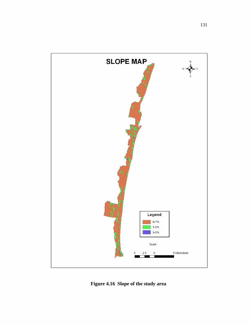
4.3.9 Slope
The study region is located on a flat coastal plain known as the Eastern Coastal Plains. Chennai has 25.60 kms of sea coast which is flat and sandy for about a km. from the shore. The bed of the sea is about 42' deep and slopes further in gradual stages for a distance of about 5 kms from the coast attaining a depth of about 63'. Width of the backshore sandy beach zone is about 4.5 km along Chennai coast. The study region has an almost flat terrain with a slope between 0-1% with certain areas having 1-3% slope (Figure 4.16). Slope of the Chennai coast at Besant Nagar is 1 in 39 upto 100 m. Kancheepuram district has a natural slope from West to East with a fall of 42 ft. Chennai city plateau is extremely flat with almost no hills. Most points of the city are within 4-5 m above the Mean Sea Level (MSL). The city is predominately flat, without any elevation. Its average slope is 0.7 m per Kilometre towards the sea.
131
Figure 4.16 Slope of the study area
132
4.3.10 Climate and Rainfall
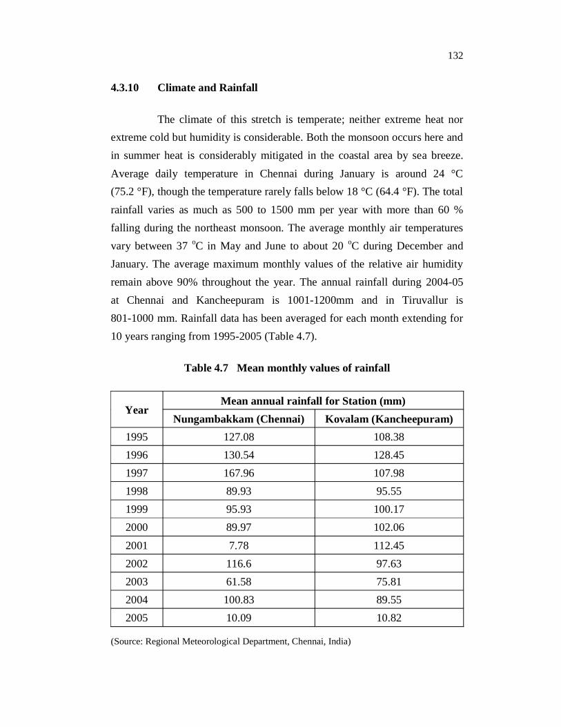
The climate of this stretch is temperate; neither extreme heat nor extreme cold but humidity is considerable. Both the monsoon occurs here and in summer heat is considerably mitigated in the coastal area by sea breeze. Average daily temperature in Chennai during January is around 24 °C (75.2 °F), though the temperature rarely falls below 18 °C (64.4 °F). The total rainfall varies as much as 500 to 1500 mm per year with more than 60 % falling during the northeast monsoon. The average monthly air temperatures vary between 37 oC in May and June to about 20 oC during December and January. The average maximum monthly values of the relative air humidity remain above 90% throughout the year. The annual rainfall during 2004-05 at Chennai and Kancheepuram is 1001-1200mm and in Tiruvallur is 801-1000 mm. Rainfall data has been averaged for each month extending for 10 years ranging from 1995-2005 (Table 4.7).
Table 4.7 Mean monthly values of rainfall
Year Mean annual rainfall for Station (mm)
Nungambakkam (Chennai) Kovalam (Kancheepuram) 1995 127.08 108.38 1996 130.54 128.45 1997 167.96 107.98 1998 89.93 95.55 1999 95.93 100.17 2000 89.97 102.06 2001 7.78 112.45 2002 116.6 97.63 2003 61.58 75.81 2004 100.83 89.55 2005 10.09 10.82
(Source: Regional Meteorological Department, Chennai, India)
133
4.3.11 Winds
The predominant wind directions in the study area are NE, ENE,
SSW, SW, ESE and SE. Based on monsoon, the climate of Chennai could be
divided into three seasons , namely, SW monsoon, NE monsoon and non-
monsoonal. During the northeast monsoon the winds blow predominantly
from the northeast with a speed of 5.8-7.5 m/s and direction of 49-87o with
respect to north, reaching a force of 7 on the Beaufort scale. During the SW
monsoon the winds blow predominantly from the southwest, with a speed is
2-12 m/s and direction of 153-263o, reaching a force of 6 on the Beaufort
scale. Thunderstorms occur throughout the year accompanied by wind gusts
of up to 130 km/hr.
4.3.12 Waves and Tides
The general wave direction in the region is 100-160o with respect to
north during SW monsoon and 60-90o during NE monsoon. Wave heights
associated with cyclones could be as high as 5 to 8 m. Tides along Chennai
coast have a period of 12 hours 20 minutes. The wave height on the Chennai
Coast during SW monsoon, range from 0.4 to 1.6 m and from 0.4 to 2.0 m
during the NE monsoon period (Narasimha Rao 1984). The tides in the region
are of semi-diurnal type with mean spring tide ranges of 1.10 m and mean
neap tide ranges of 0.8 m based on characteristics of the tide on the Chennai
coast with respect to Chart Datum specified by the National hydrographic
office, India. The significant wave heights at the Chennai Port have been
collected for 2000-2005 (Table 4.8).
134
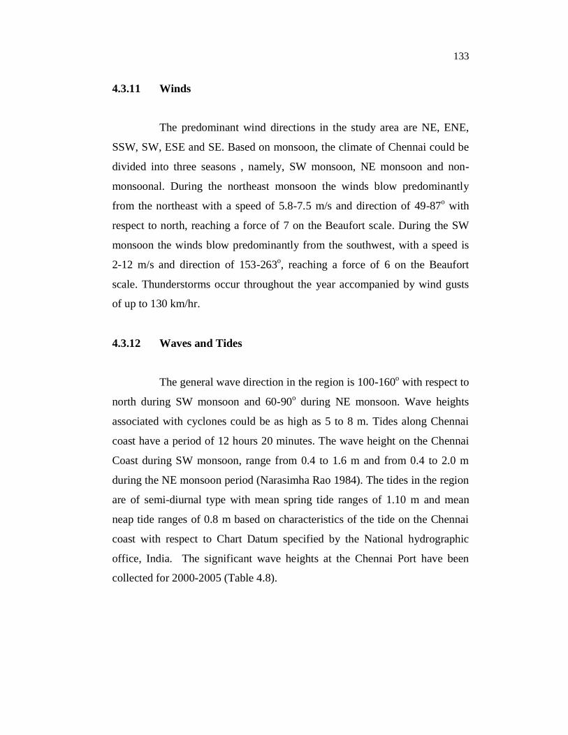
Table 4.8 Significant Wave height observations (in metres)
Year 2000 2001 2002 2003 2004 2005 Month Height Height Height Height Height Height
January * 0.75 0.90 1.00 1.00 1.00 February * 0.60 0.60 0.90 1.00 1.00 March 0.75 0.60 0.75 1.00 1.00 1.00 April 1.00 0.60 1.00 0.90 1.00 1.00 May 0.75 0.60 0.90 1.00 1.00 1.00 June 1.25 0.60 0.75 1.00 0.75 1.00
July 0.90 0.75 1.00 1.00 1.00 1.00 August 0.60 0.60 0.90 0.90 1.00 1.00 September 0.75 0.60 0.75 0.90 1.00 1.00 October 1.00 1.00 0.90 1.00 1.00 1.5 November 2.5-3.0 1.00 1.50 1.50 1.00 1.5 December 0.75 1.00 1.00 2.5-3.0 1.00 1.5
* Data not available (Source: Port Trust of India)
The wave conditions in the vicinity of Chennai coast is strongly
influenced by the monsoons blowing over the coast. The directions of wave
approach coincide with the monsoonal seasons and the heights are also
influenced by the cyclonic conditions prevailing during the monsoons. The
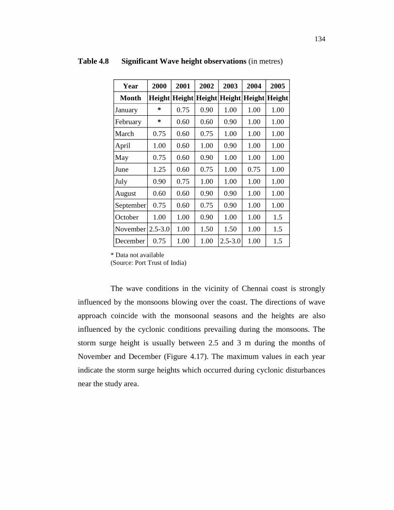
storm surge height is usually between 2.5 and 3 m during the months of
November and December (Figure 4.17). The maximum values in each year
indicate the storm surge heights which occurred during cyclonic disturbances
near the study area.
135
Significant Wave Height
00.5
11.5
22.5
33.5
Month
200020012002200320042005
Figure 4.17 Significant Wave Heights during 2000-2005
The wave heights inferred by Sundar (1986) from visually observed
wave data of Chennai Port trust from April 1974 to March 1984 are of the
range 0.4 to 2.5 m and wave periods vary between 5 and 15 secs. The study
region could receive waves as high as 8m during the NE monsoon and during
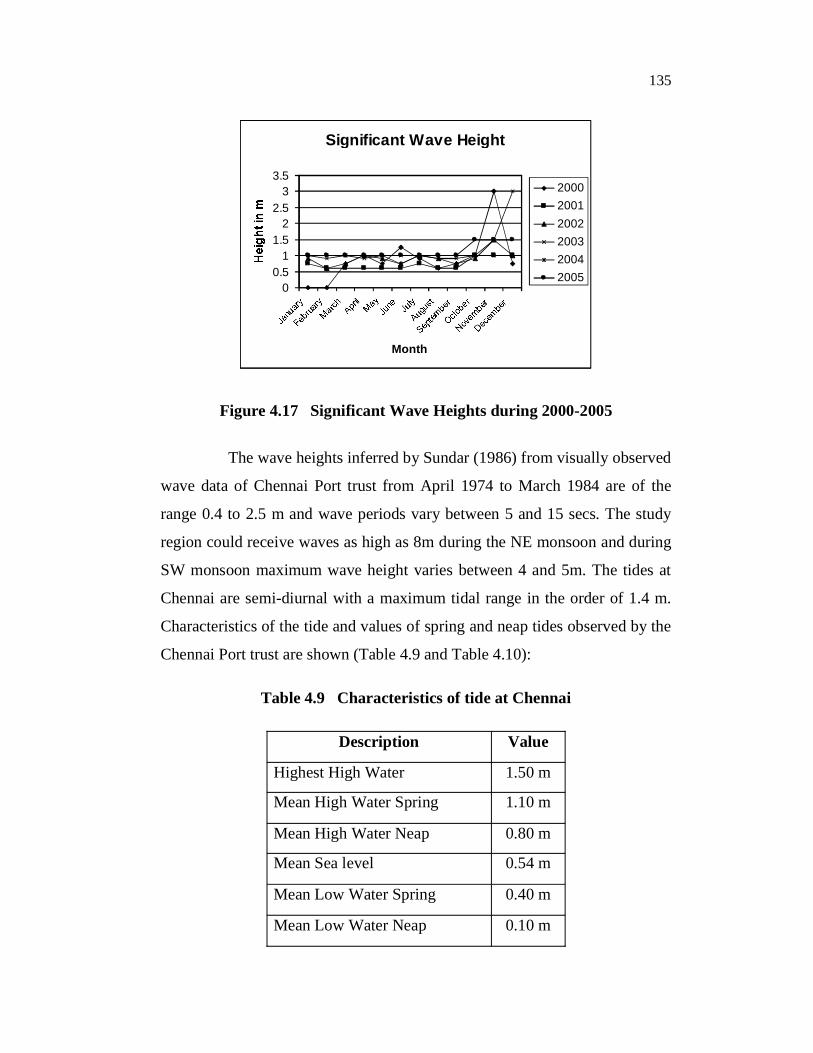
SW monsoon maximum wave height varies between 4 and 5m. The tides at
Chennai are semi-diurnal with a maximum tidal range in the order of 1.4 m.
Characteristics of the tide and values of spring and neap tides observed by the
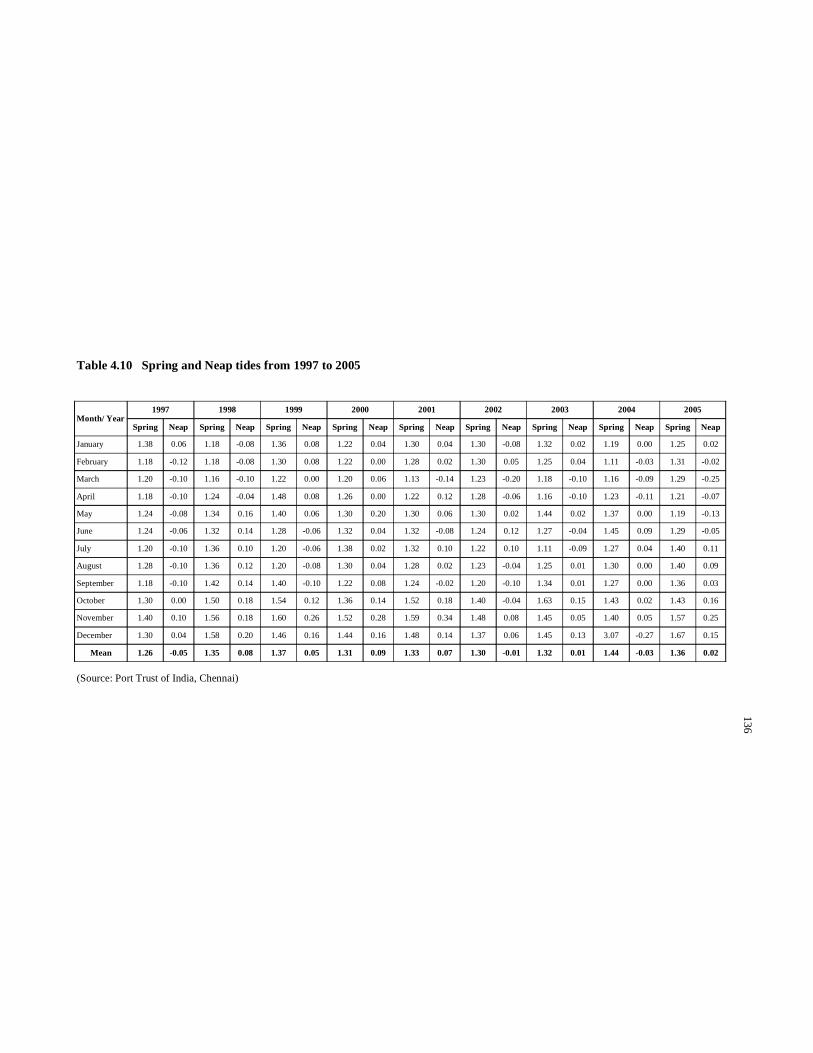
Chennai Port trust are shown (Table 4.9 and Table 4.10):
Table 4.9 Characteristics of tide at Chennai
Description Value
Highest High Water 1.50 m
Mean High Water Spring 1.10 m
Mean High Water Neap 0.80 m
Mean Sea level 0.54 m
Mean Low Water Spring 0.40 m
Mean Low Water Neap 0.10 m
136
Table 4.10 Spring and Neap tides from 1997 to 2005
Month/ Year 1997 1998 1999 2000 2001 2002 2003 2004 2005
Spring Neap Spring Neap Spring Neap Spring Neap Spring Neap Spring Neap Spring Neap Spring Neap Spring Neap
January 1.38 0.06 1.18 -0.08 1.36 0.08 1.22 0.04 1.30 0.04 1.30 -0.08 1.32 0.02 1.19 0.00 1.25 0.02
February 1.18 -0.12 1.18 -0.08 1.30 0.08 1.22 0.00 1.28 0.02 1.30 0.05 1.25 0.04 1.11 -0.03 1.31 -0.02
March 1.20 -0.10 1.16 -0.10 1.22 0.00 1.20 0.06 1.13 -0.14 1.23 -0.20 1.18 -0.10 1.16 -0.09 1.29 -0.25
April 1.18 -0.10 1.24 -0.04 1.48 0.08 1.26 0.00 1.22 0.12 1.28 -0.06 1.16 -0.10 1.23 -0.11 1.21 -0.07
May 1.24 -0.08 1.34 0.16 1.40 0.06 1.30 0.20 1.30 0.06 1.30 0.02 1.44 0.02 1.37 0.00 1.19 -0.13
June 1.24 -0.06 1.32 0.14 1.28 -0.06 1.32 0.04 1.32 -0.08 1.24 0.12 1.27 -0.04 1.45 0.09 1.29 -0.05
July 1.20 -0.10 1.36 0.10 1.20 -0.06 1.38 0.02 1.32 0.10 1.22 0.10 1.11 -0.09 1.27 0.04 1.40 0.11
August 1.28 -0.10 1.36 0.12 1.20 -0.08 1.30 0.04 1.28 0.02 1.23 -0.04 1.25 0.01 1.30 0.00 1.40 0.09
September 1.18 -0.10 1.42 0.14 1.40 -0.10 1.22 0.08 1.24 -0.02 1.20 -0.10 1.34 0.01 1.27 0.00 1.36 0.03
October 1.30 0.00 1.50 0.18 1.54 0.12 1.36 0.14 1.52 0.18 1.40 -0.04 1.63 0.15 1.43 0.02 1.43 0.16
November 1.40 0.10 1.56 0.18 1.60 0.26 1.52 0.28 1.59 0.34 1.48 0.08 1.45 0.05 1.40 0.05 1.57 0.25
December 1.30 0.04 1.58 0.20 1.46 0.16 1.44 0.16 1.48 0.14 1.37 0.06 1.45 0.13 3.07 -0.27 1.67 0.15
Mean 1.26 -0.05 1.35 0.08 1.37 0.05 1.31 0.09 1.33 0.07 1.30 -0.01 1.32 0.01 1.44 -0.03 1.36 0.02
(Source: Port Trust of India, Chennai)
137
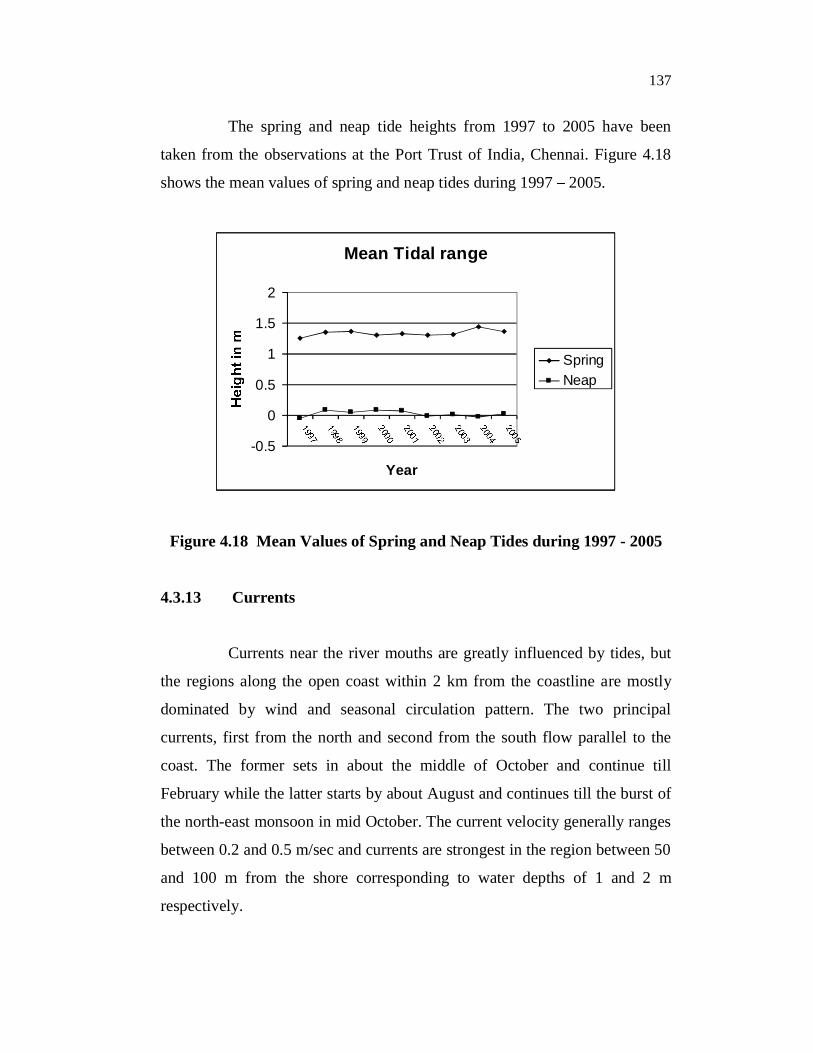
The spring and neap tide heights from 1997 to 2005 have been
taken from the observations at the Port Trust of India, Chennai. Figure 4.18
shows the mean values of spring and neap tides during 1997 2005.
Mean Tidal range
-0.5
0
0.5
1
1.5
2
Year
Spring Neap
Figure 4.18 Mean Values of Spring and Neap Tides during 1997 - 2005
4.3.13 Currents
Currents near the river mouths are greatly influenced by tides, but
the regions along the open coast within 2 km from the coastline are mostly
dominated by wind and seasonal circulation pattern. The two principal
currents, first from the north and second from the south flow parallel to the
coast. The former sets in about the middle of October and continue till
February while the latter starts by about August and continues till the burst of
the north-east monsoon in mid October. The current velocity generally ranges
between 0.2 and 0.5 m/sec and currents are strongest in the region between 50
and 100 m from the shore corresponding to water depths of 1 and 2 m
respectively.
138
4.4 SOCIAL SCENARIO
4.4.1 Infrastructure
The Chennai city is served by an international airport and two
major ports and it is connected to the rest of the country by five national
highways and two railway terminals. The Chennai Metropolitan area has a
broad industrial base in the automobile, technology, hardware manufacturing,
and healthcare industries. The region is well connected by roads, rail network
including the Mass Rapid Transit System (MRTS), bridges and
telecommunications. The road and rail alignments from satellite imagery and
SOI map have been mapped and symbolized as per the NRIS classification
scheme (NRIS 1997). All roads have been classified into specified categories,
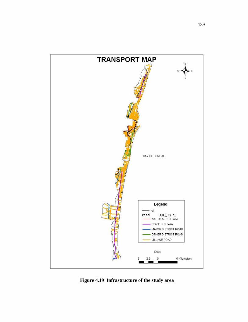
while all rail tracks have been shown as single category (Figure 4.19). The
port of Chennai is the largest and most advanced port facility within the
region, reportedly handling 20% of all throughputs for India (ASCE 2005).
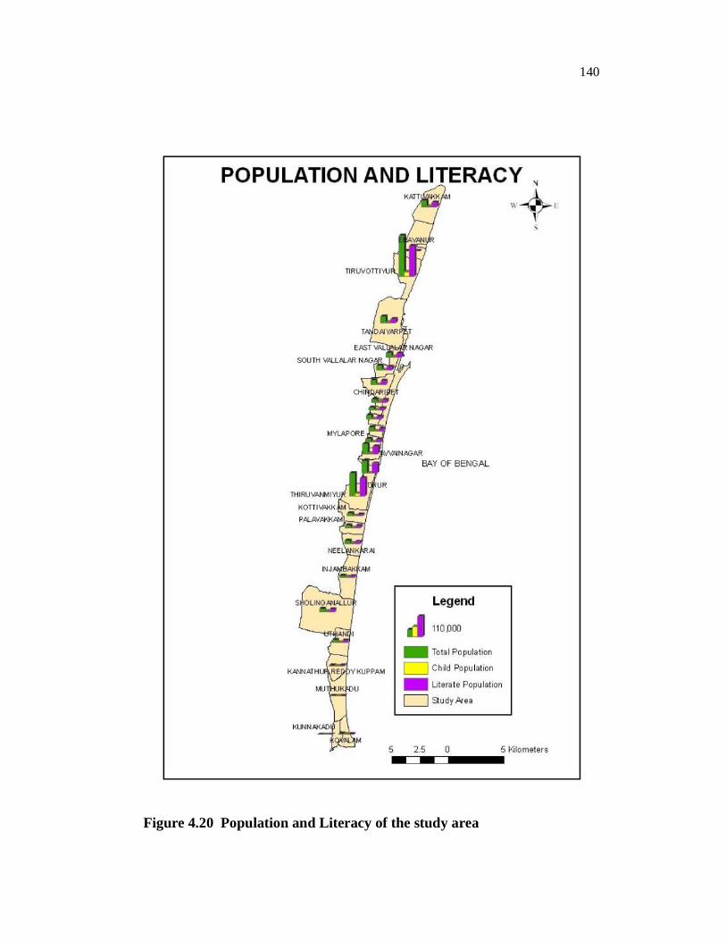
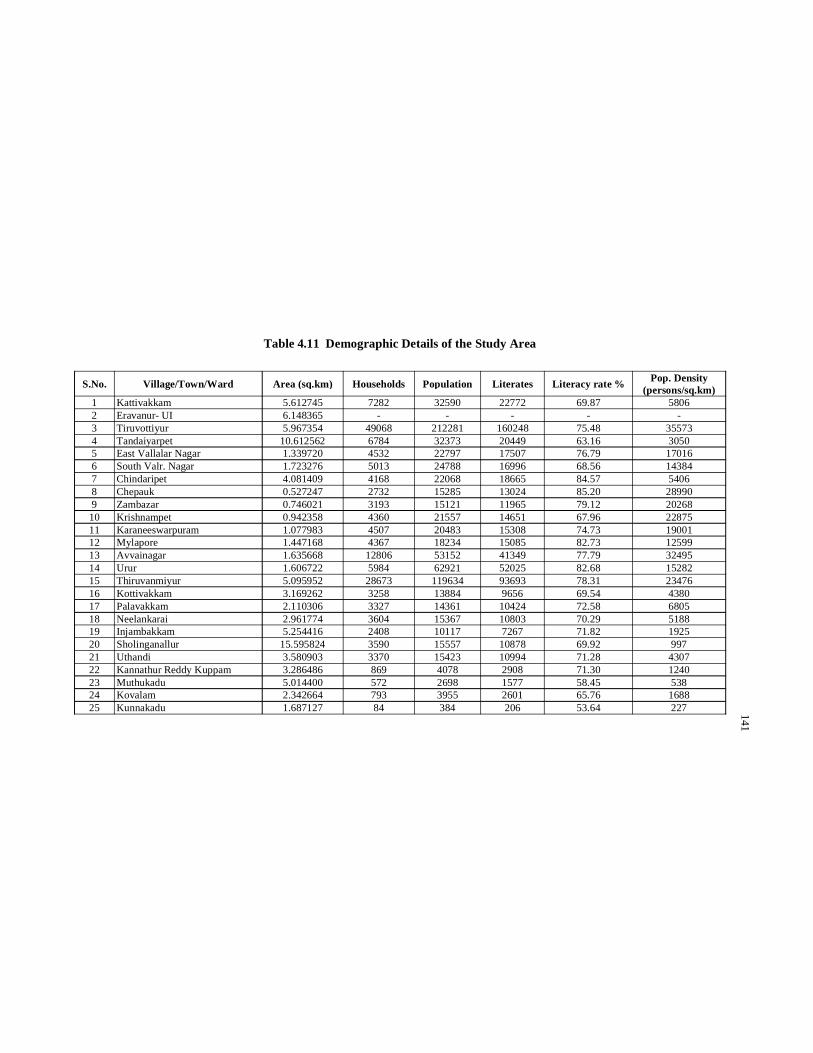
4.4.2 Demography
Chennai has an estimated population of 7.5 million (2008)
(www.world-gazetteer.com), making it the fourth largest metropolitan city in
India. The overall population density of Tamil Nadu is 6,351 per km² (Census
of India, 2001), whereas the density varies for the individual villages and
towns (Table 4.11). The population density has been calculated for each unit
and classified by Natural breaks (Jenks) method. The five classes are based on
natural groupings inherent in the data. The break points have been identified
using ArcMap software by picking the class breaks that best group similar
values and maximize the differences between classes. The features are divided
into classes whose boundaries are set where there are relatively big jumps in
the data values (Figure 4.20).
139
Figure 4.19 Infrastructure of the study area
140
Figure 4.20 Population and Literacy of the study area
141
Table 4.11 Demographic Details of the Study Area
S.No. Village/Town/Ward Area (sq.km) Households Population Literates Literacy rate % Pop. Density (persons/sq.km)
1 Kattivakkam 5.612745 7282 32590 22772 69.87 5806 2 Eravanur- UI 6.148365 - - - - - 3 Tiruvottiyur 5.967354 49068 212281 160248 75.48 35573 4 Tandaiyarpet 10.612562 6784 32373 20449 63.16 3050 5 East Vallalar Nagar 1.339720 4532 22797 17507 76.79 17016 6 South Valr. Nagar 1.723276 5013 24788 16996 68.56 14384 7 Chindaripet 4.081409 4168 22068 18665 84.57 5406 8 Chepauk 0.527247 2732 15285 13024 85.20 28990 9 Zambazar 0.746021 3193 15121 11965 79.12 20268 10 Krishnampet 0.942358 4360 21557 14651 67.96 22875 11 Karaneeswarpuram 1.077983 4507 20483 15308 74.73 19001 12 Mylapore 1.447168 4367 18234 15085 82.73 12599 13 Avvainagar 1.635668 12806 53152 41349 77.79 32495 14 Urur 1.606722 5984 62921 52025 82.68 15282 15 Thiruvanmiyur 5.095952 28673 119634 93693 78.31 23476 16 Kottivakkam 3.169262 3258 13884 9656 69.54 4380 17 Palavakkam 2.110306 3327 14361 10424 72.58 6805 18 Neelankarai 2.961774 3604 15367 10803 70.29 5188 19 Injambakkam 5.254416 2408 10117 7267 71.82 1925 20 Sholinganallur 15.595824 3590 15557 10878 69.92 997 21 Uthandi 3.580903 3370 15423 10994 71.28 4307 22 Kannathur Reddy Kuppam 3.286486 869 4078 2908 71.30 1240 23 Muthukadu 5.014400 572 2698 1577 58.45 538 24 Kovalam 2.342664 793 3955 2601 65.76 1688 25 Kunnakadu 1.687127 84 384 206 53.64 227
142
4.4.3 Human Development
The notion of human well-being includes not only the consumption
of goods and services but also the accessibility of all sections of the
population to the basic necessities of a productive and socially meaningful
life. The conventional measures of well-being, such as Gross Domestic
Product (GDP) or per capita income and their alternatives are inherently
limited in capturing the wider aspects of the process of development.
The human development indicators of any country with respect to
hazard risk management include GDP/capita , Gini coefficient, Literacy,
Incidence of poverty, Life expectancy, Insurance mechanisms, Degree of
urbanization, Access to public health facilities, education, Community
organisations, planning regulations, warning and protection from natural
hazards, Institutional and decision-making frameworks and political stability
(UNDP 2000). The indicators have been grouped under various categories
such as economic attainment, educational attainment, health attainment and
demography. The human development index for the whole of country has
been computed as 0.619 by the United Nations Development Programme.
4.5 HAZARD SCENARIO
The major coastal hazards affecting the study area, as seen from
previous literature and historical data, are: Cyclones, Storm surges,
Earthquakes, Tsunami, Coastal Erosion and Sea level rise. Hazards associated
with volcanic eruptions including lava flows, falling ash and projectiles,
mudflows, and toxic gases and landslides including slides, falls, and flows of
unconsolidated materials have not occurred in the known history of the study
area. Hence these hazards are not considered for the present analysis.
143
In India, the climate and weather are dominated by the largest
seasonal mode of precipitation in the world, due to the summer monsoon
circulation. Indeed, rainfall during a typical monsoon season is by no means
uniformly distributed in time on a regional/local scale, but is marked by a few
active spells separated by weak monsoon or break periods of little or no rain.
Thus, the daily distribution of rainfall at the local level has important
consequences in terms of the occurrence of extremes.
Areas that receive up to 60 centimeters of rainfall annually are the
most drought-prone. Hence, after a thorough observation of the rainfall data
of the study area, impacts of precipitation variability have not been considered
for the present analysis.
4.5.1 Cyclones and Storm Surges
The Bay of Bengal is one of the major centres of the world for
breeding of tropical storms. Cyclones over the Bay of Bengal usually move
westward, northwestward, or northward and cross the East coast of India.
Frequency of formation of cyclones is 5-6 times more in Bay of Bengal as
compared to Arabian Sea (IMD 1979). The cyclone affected areas of the
country are classified in 50 and 55 m/s zones. During cyclonic period, wind
speed often exceeds 100 km/h (27.8 m/s).
While the total frequency of cyclonic storms that form over the Bay
of Bengal has remained almost constant over the period 1887-1997, an
increase in the frequency of severe cyclonic storms appears to have taken
place in recent decades. Cyclone data over the Bay of Bengal since 1891
indicates that on average, a moderate to severe cyclone hits the Tamil Nadu
coast every two years (Table 4.12).
144
A storm surge of approximately once in 5 years has a height of
about 7 m. The Tamil Nadu coast has observed surge heights in the range of
1 to 6 m. The height of the surges is limited, due to the depths in the bay, to a
maximum of about 12 m. The frequency of a wave with a height of 12 m is
approximately once per 20 years. The probable maximum surge height along
the coastal area of Chennai district according to the vulnerability atlas of India
1997) is found to be 5.45m.
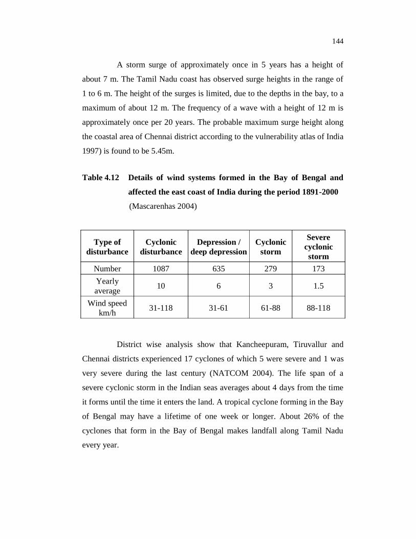
Table 4.12 Details of wind systems formed in the Bay of Bengal and
affected the east coast of India during the period 1891-2000
(Mascarenhas 2004)
Type of disturbance
Cyclonic disturbance
Depression / deep depression
Cyclonic storm
Severe cyclonic storm
Number 1087 635 279 173 Yearly average 10 6 3 1.5
Wind speed km/h 31-118 31-61 61-88 88-118
District wise analysis show that Kancheepuram, Tiruvallur and
Chennai districts experienced 17 cyclones of which 5 were severe and 1 was
very severe during the last century (NATCOM 2004). The life span of a
severe cyclonic storm in the Indian seas averages about 4 days from the time
it forms until the time it enters the land. A tropical cyclone forming in the Bay
of Bengal may have a lifetime of one week or longer. About 26% of the
cyclones that form in the Bay of Bengal makes landfall along Tamil Nadu
every year.
145
4.5.1.1 Cyclone tracks
Hazard map for cyclones has been prepared by using data inputs of
past climatological records. Historic Data about cyclonic disturbances
affecting the study region and its surrounding area from 1945 to 2006 have
been compiled (Data courtesy: Joint Typhoon Warning Center;
http://weather.unisys.com).
The Joint Typhoon Warning Center, Pearl Harbour Hawaii, is
responsible for providing tropical cyclone forecasts. Data from geostationary
satellites as well as polar and equatorial orbiting satellites are used to assess
synoptic features and to ascertain cyclone position, intensity and size.
Increased use of microwave imagery and scatterometer data has also been
done to improve the temporal and spatial continuity of analysis.
Some of the satellites from which data is collected include GOES
(Geostationary Operational Environmental Satellites), DMSP (Defense
Meteorological Satellite Program) and NOAA (National Oceanic and
Atmospheric Administration) and sensors including TRMM (Tropical
Rainfall Measuring Mission) and SSM/I (Special Sensor Microwave Imager).
The satellite data along with surface observations, upper air
observations, satellite derived winds, radar observations, aircraft observations
and model forecast output help in maintaining a continuous meteorological
watch over the Indian Ocean.
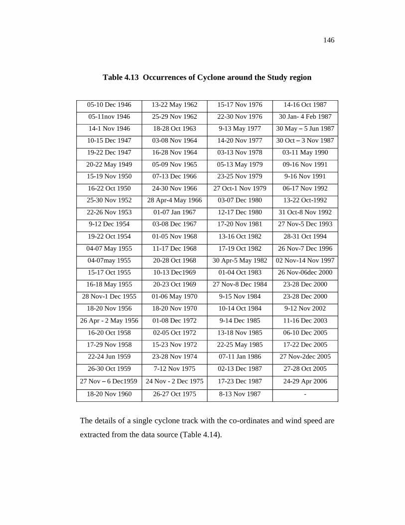
A text based table of tracking information denoting the position in
latitude and longitude, maximum sustained winds in knots, and central
pressure in millibars and the map depicting the cyclone tracks has been
collected for each track (Table 4.13).
146
Table 4.13 Occurrences of Cyclone around the Study region
05-10 Dec 1946 13-22 May 1962 15-17 Nov 1976 14-16 Oct 1987
05-11nov 1946 25-29 Nov 1962 22-30 Nov 1976 30 Jan- 4 Feb 1987
14-1 Nov 1946 18-28 Oct 1963 9-13 May 1977 30 May 5 Jun 1987
10-15 Dec 1947 03-08 Nov 1964 14-20 Nov 1977 30 Oct 3 Nov 1987
19-22 Dec 1947 16-28 Nov 1964 03-13 Nov 1978 03-11 May 1990
20-22 May 1949 05-09 Nov 1965 05-13 May 1979 09-16 Nov 1991
15-19 Nov 1950 07-13 Dec 1966 23-25 Nov 1979 9-16 Nov 1991
16-22 Oct 1950 24-30 Nov 1966 27 Oct-1 Nov 1979 06-17 Nov 1992
25-30 Nov 1952 28 Apr-4 May 1966 03-07 Dec 1980 13-22 Oct-1992
22-26 Nov 1953 01-07 Jan 1967 12-17 Dec 1980 31 Oct-8 Nov 1992
9-12 Dec 1954 03-08 Dec 1967 17-20 Nov 1981 27 Nov-5 Dec 1993
19-22 Oct 1954 01-05 Nov 1968 13-16 Oct 1982 28-31 Oct 1994
04-07 May 1955 11-17 Dec 1968 17-19 Oct 1982 26 Nov-7 Dec 1996
04-07may 1955 20-28 Oct 1968 30 Apr-5 May 1982 02 Nov-14 Nov 1997
15-17 Oct 1955 10-13 Dec1969 01-04 Oct 1983 26 Nov-06dec 2000
16-18 May 1955 20-23 Oct 1969 27 Nov-8 Dec 1984 23-28 Dec 2000
28 Nov-1 Dec 1955 01-06 May 1970 9-15 Nov 1984 23-28 Dec 2000
18-20 Nov 1956 18-20 Nov 1970 10-14 Oct 1984 9-12 Nov 2002
26 Apr - 2 May 1956 01-08 Dec 1972 9-14 Dec 1985 11-16 Dec 2003
16-20 Oct 1958 02-05 Oct 1972 13-18 Nov 1985 06-10 Dec 2005
17-29 Nov 1958 15-23 Nov 1972 22-25 May 1985 17-22 Dec 2005
22-24 Jun 1959 23-28 Nov 1974 07-11 Jan 1986 27 Nov-2dec 2005
26-30 Oct 1959 7-12 Nov 1975 02-13 Dec 1987 27-28 Oct 2005
27 Nov 6 Dec1959 24 Nov - 2 Dec 1975 17-23 Dec 1987 24-29 Apr 2006
18-20 Nov 1960 26-27 Oct 1975 8-13 Nov 1987 -
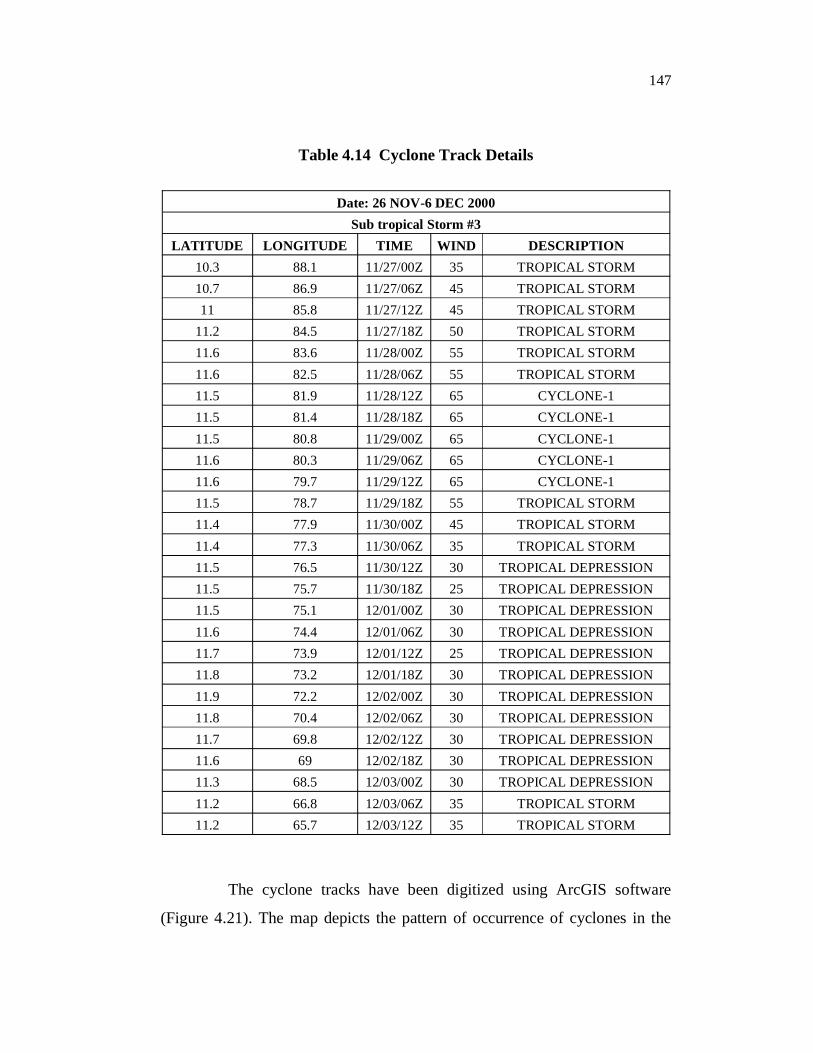
The details of a single cyclone track with the co-ordinates and wind speed are
extracted from the data source (Table 4.14).
147
Table 4.14 Cyclone Track Details
Date: 26 NOV-6 DEC 2000 Sub tropical Storm #3
LATITUDE LONGITUDE TIME WIND DESCRIPTION 10.3 88.1 11/27/00Z 35 TROPICAL STORM 10.7 86.9 11/27/06Z 45 TROPICAL STORM 11 85.8 11/27/12Z 45 TROPICAL STORM
11.2 84.5 11/27/18Z 50 TROPICAL STORM 11.6 83.6 11/28/00Z 55 TROPICAL STORM 11.6 82.5 11/28/06Z 55 TROPICAL STORM 11.5 81.9 11/28/12Z 65 CYCLONE-1 11.5 81.4 11/28/18Z 65 CYCLONE-1 11.5 80.8 11/29/00Z 65 CYCLONE-1 11.6 80.3 11/29/06Z 65 CYCLONE-1 11.6 79.7 11/29/12Z 65 CYCLONE-1 11.5 78.7 11/29/18Z 55 TROPICAL STORM 11.4 77.9 11/30/00Z 45 TROPICAL STORM 11.4 77.3 11/30/06Z 35 TROPICAL STORM 11.5 76.5 11/30/12Z 30 TROPICAL DEPRESSION 11.5 75.7 11/30/18Z 25 TROPICAL DEPRESSION 11.5 75.1 12/01/00Z 30 TROPICAL DEPRESSION 11.6 74.4 12/01/06Z 30 TROPICAL DEPRESSION 11.7 73.9 12/01/12Z 25 TROPICAL DEPRESSION 11.8 73.2 12/01/18Z 30 TROPICAL DEPRESSION 11.9 72.2 12/02/00Z 30 TROPICAL DEPRESSION 11.8 70.4 12/02/06Z 30 TROPICAL DEPRESSION 11.7 69.8 12/02/12Z 30 TROPICAL DEPRESSION 11.6 69 12/02/18Z 30 TROPICAL DEPRESSION 11.3 68.5 12/03/00Z 30 TROPICAL DEPRESSION 11.2 66.8 12/03/06Z 35 TROPICAL STORM 11.2 65.7 12/03/12Z 35 TROPICAL STORM
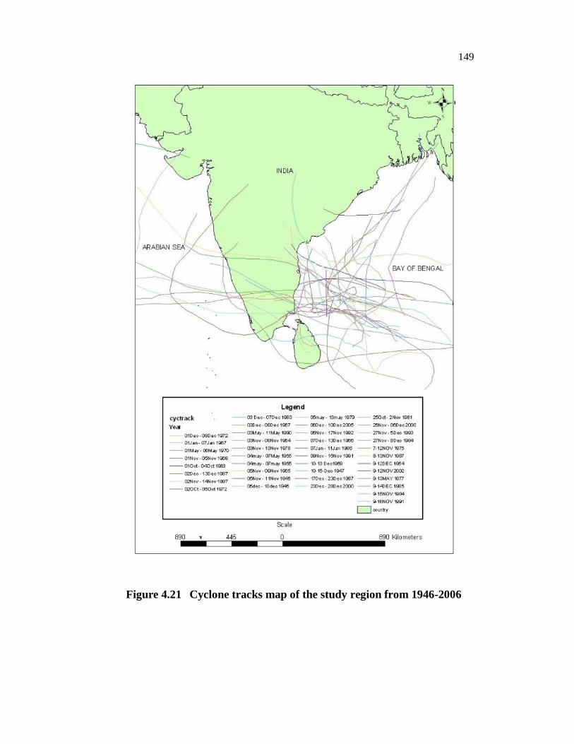
The cyclone tracks have been digitized using ArcGIS software
(Figure 4.21). The map depicts the pattern of occurrence of cyclones in the
148
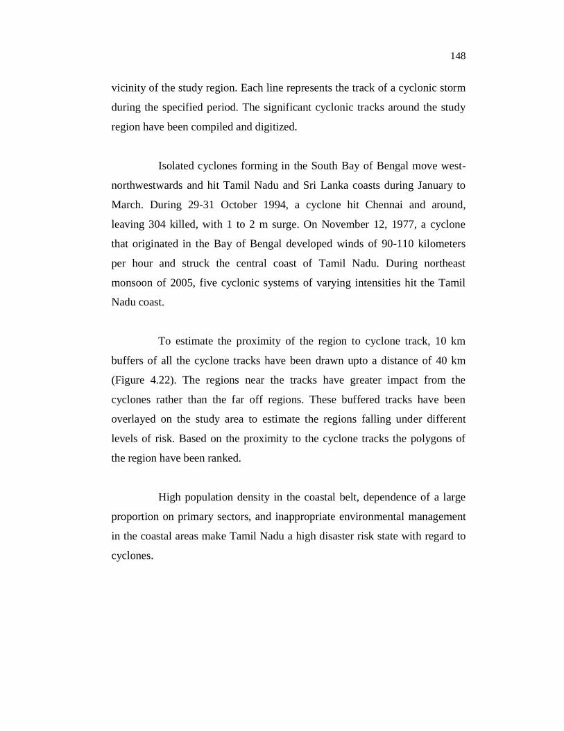
vicinity of the study region. Each line represents the track of a cyclonic storm
during the specified period. The significant cyclonic tracks around the study
region have been compiled and digitized.
Isolated cyclones forming in the South Bay of Bengal move west-
northwestwards and hit Tamil Nadu and Sri Lanka coasts during January to
March. During 29-31 October 1994, a cyclone hit Chennai and around,
leaving 304 killed, with 1 to 2 m surge. On November 12, 1977, a cyclone
that originated in the Bay of Bengal developed winds of 90-110 kilometers
per hour and struck the central coast of Tamil Nadu. During northeast
monsoon of 2005, five cyclonic systems of varying intensities hit the Tamil
Nadu coast.
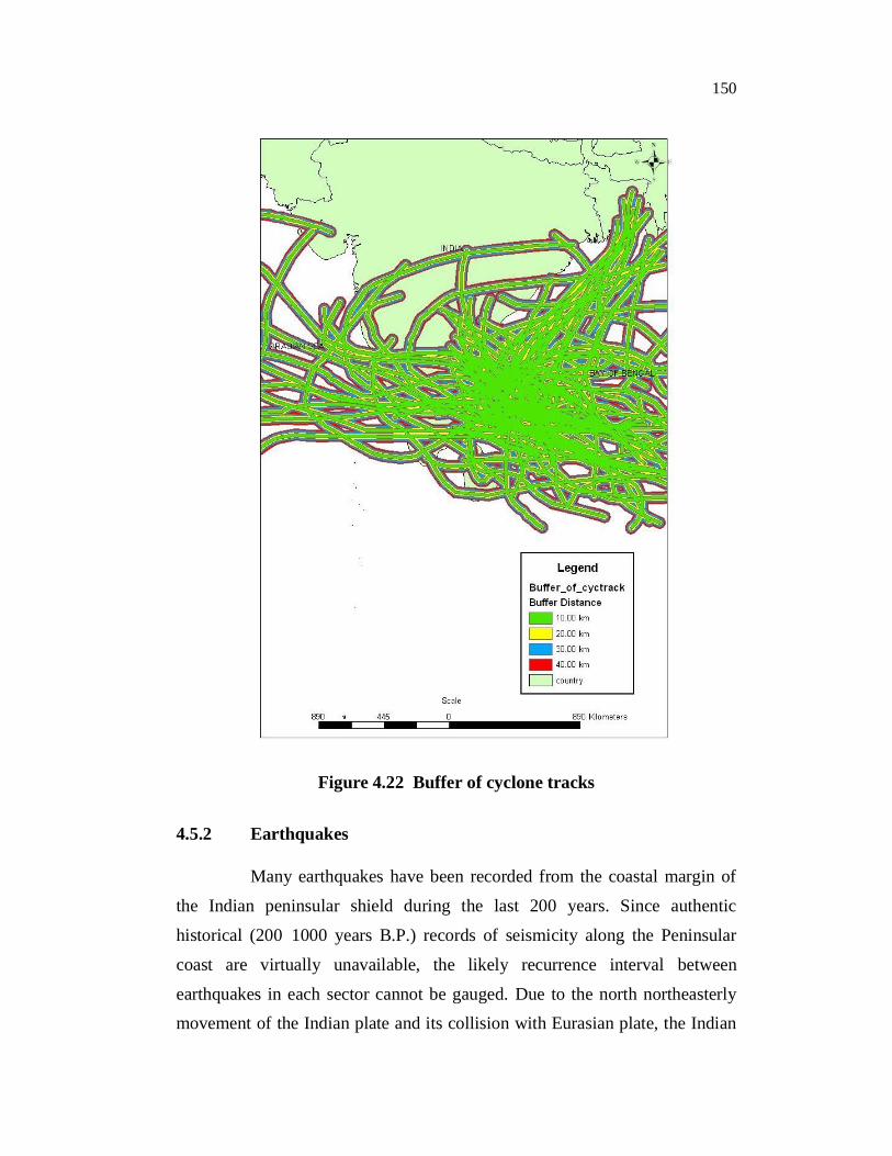
To estimate the proximity of the region to cyclone track, 10 km
buffers of all the cyclone tracks have been drawn upto a distance of 40 km
(Figure 4.22). The regions near the tracks have greater impact from the
cyclones rather than the far off regions. These buffered tracks have been
overlayed on the study area to estimate the regions falling under different
levels of risk. Based on the proximity to the cyclone tracks the polygons of
the region have been ranked.
High population density in the coastal belt, dependence of a large
proportion on primary sectors, and inappropriate environmental management
in the coastal areas make Tamil Nadu a high disaster risk state with regard to
cyclones.
149
Figure 4.21 Cyclone tracks map of the study region from 1946-2006
150
Figure 4.22 Buffer of cyclone tracks
4.5.2 Earthquakes
Many earthquakes have been recorded from the coastal margin of
the Indian peninsular shield during the last 200 years. Since authentic
historical (200 1000 years B.P.) records of seismicity along the Peninsular
coast are virtually unavailable, the likely recurrence interval between
earthquakes in each sector cannot be gauged. Due to the north northeasterly movement of the Indian plate and its collision with Eurasian plate, the Indian
151
plate has subducted and the huge Himalayan Mountains have risen up. At the same time, the Indian plate is not able to move northerly as the Himalayan
Mountains are obstructing the same. Hence, the Indian plate is whirling like a
worm with a series of East-west trending alternating cymatogenic arches and
deeps from south to north viz: Mangalore - Chennai (Ramasamy et al 1987).
According to GSHAP (Global Seismic Hazard Assessment
Programme) data, the state of Tamil Nadu falls mostly in a region of low seismic hazard with the exception of western border areas that lie in a low to
moderate hazard zone. As per the 2002 Bureau of Indian Standards (BIS)
map, Tamil Nadu falls in Zones II & III. The city of Chennai, formerly in
zone II now lies in zone III (ASC 2006). Historically, parts of this region have experienced seismic activity in the M5.0 range. Recent tremors occurred in
Chennai due to the 2001 Bhuj earthquake (Mw 7.6), 2001 Pondicherry
earthquake (Mw 5.6), and the 2004 Sumatra earthquake
(Mw 9.1). The Earthquake catalogues of National Earthquake Information Catalogue (NEIC), USA shows that 65 earthquakes have occurred within 300
km from Chennai and 450 earthquakes have occurred in Peninsular India since 1800 A.D. (Table 4.15).
The peninsular Indian landmass has been considered to be stable and a region of slight seismicity. The geological framework of the region is
the cumulative effect of geodynamics sequences ranging from Early
Precambrian crustal evolution to young volcanism over its northwest segment
(Parvez et al 2003). It is interesting to note that in South India, barring a few,
majority of earthquake epicenters are confined to the high-grade granulite terrain. The few events in the granite- gneiss greenstone terrain are
distributed on either side of the NW SE Chennai Mumbai line. Also, the
large area confined between north of Chennai line and south of Tapti fault comprising Deccan trap and gneisses is devoid of any seismic activity
(Murthy 2002).
152
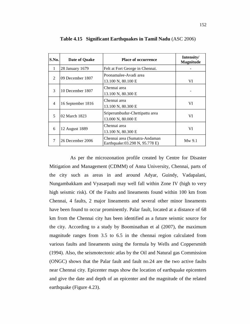
Table 4.15 Significant Earthquakes in Tamil Nadu (ASC 2006)
S.No. Date of Quake Place of occurrence Intensity/ Magnitude
1 28 January 1679 Felt at Fort George in Chennai. -
2 09 December 1807 Poonamalee-Avadi area 13.100 N, 80.100 E
VI
3 10 December 1807 Chennai area 13.100 N, 80.300 E
-
4 16 September 1816 Chennai area 13.100 N, 80.300 E
VI
5 02 March 1823 Sriperumbudur-Chettipattu area 13.000 N, 80.000 E
VI
6 12 August 1889 Chennai area 13.100 N, 80.300 E
VI
7 26 December 2006 Chennai area (Sumatra-Andaman Earthquake:03.298 N, 95.778 E) Mw 9.1
As per the microzonation profile created by Centre for Disaster
Mitigation and Management (CDMM) of Anna University, Chennai, parts of
the city such as areas in and around Adyar, Guindy, Vadapalani,
Nungambakkam and Vyasarpadi may well fall within Zone IV (high to very
high seismic risk). Of the Faults and lineaments found within 100 km from
Chennai, 4 faults, 2 major lineaments and several other minor lineaments
have been found to occur prominently. Palar fault, located at a distance of 68
km from the Chennai city has been identified as a future seismic source for
the city. According to a study by Boominathan et al (2007), the maximum
magnitude ranges from 3.5 to 6.5 in the chennai region calculated from
various faults and lineaments using the formula by Wells and Coppersmith
(1994). Also, the seismotectonic atlas by the Oil and Natural gas Commission
(ONGC) shows that the Palar fault and fault no.24 are the two active faults
near Chennai city. Epicenter maps show the location of earthquake epicenters
and give the date and depth of an epicenter and the magnitude of the related
earthquake (Figure 4.23).
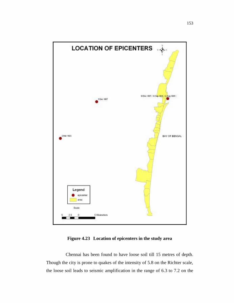
153
Figure 4.23 Location of epicenters in the study area
Chennai has been found to have loose soil till 15 metres of depth.
Though the city is prone to quakes of the intensity of 5.8 on the Richter scale,
the loose soil leads to seismic amplification in the range of 6.3 to 7.2 on the
154
Richter scale according to a study by CDMM, Anna University, Chennai.
High seismic hazard areas have been found distributed in the whole of
Chennai with North Chennai having the largest area of very high to high
hazard prone areas.
4.5.3 Tsunamis
On 26th December 2004, the Indian coastline experienced the most
devastating tsunami in recorded history. The tsunami was triggered by an
earthquake of magnitude Mw 9.3 at 3.316°N, 95.854°E off the coast of
Sumatra in the Indonesian Archipelago at 06:29 hrs making it the most
powerful in the world in the last 40 years. More than 80% of the world's
tsunamis were caused by earthquakes and over 60% of these were observed in
the Pacific where large earthquakes occur as tectonic plates are subducted
along the Pacific Ring of Fire. Tsunamis have caused damage locally in all
ocean basins. On the average, there are two tsunamis per year somewhere in
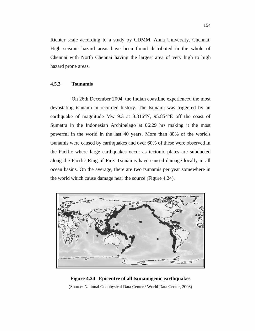
the world which cause damage near the source (Figure 4.24).
Figure 4.24 Epicentre of all tsunamigenic earthquakes (Source: National Geophysical Data Center / World Data Center, 2008)
155
For the Indian region, two potential sources of tsunami have been identified,
namely Mekran coast and Andaman to Sumatra region. The Indian coast was
affected five times due to tsunamis during the last 122 years (1883-2004).
While the frequency of tsunamis in the Pacific Ocean is five per year,
tsunamis in India have a lesser frequency of once in 24 years. The Maximum
inundation limit of different villages of the study area measured during the
recent tsunami of 2004 range from 100 to 500 m and the run up ranges from
1 to 4 m. there has been no significant damage to the Chennai port due to the
tsunami. Some of the tsunamis that have occurred in the past have been
documented (Table 4.16)
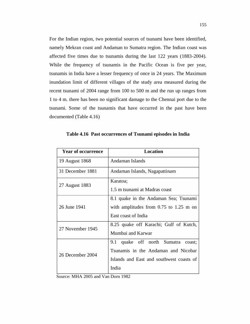
Table 4.16 Past occurrences of Tsunami episodes in India
Year of occurrence Location
19 August 1868 Andaman Islands
31 December 1881 Andaman Islands, Nagapattinam
27 August 1883 Karatoa;
1.5 m tsunami at Madras coast
26 June 1941
8.1 quake in the Andaman Sea; Tsunami
with amplitudes from 0.75 to 1.25 m on
East coast of India
27 November 1945 8.25 quake off Karachi; Gulf of Kutch,
Mumbai and Karwar
26 December 2004
9.1 quake off north Sumatra coast;
Tsunamis in the Andaman and Nicobar
Islands and East and southwest coasts of
India
Source: MHA 2005 and Van Dorn 1982
156
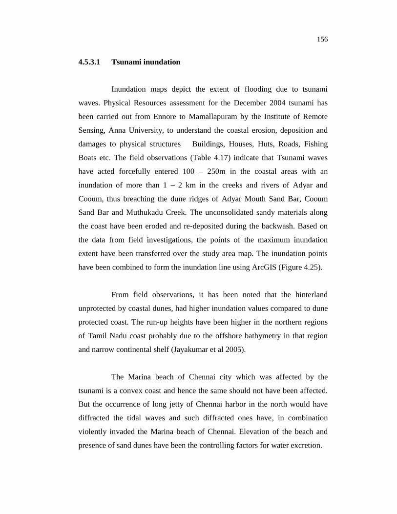
4.5.3.1 Tsunami inundation
Inundation maps depict the extent of flooding due to tsunami
waves. Physical Resources assessment for the December 2004 tsunami has
been carried out from Ennore to Mamallapuram by the Institute of Remote
Sensing, Anna University, to understand the coastal erosion, deposition and
damages to physical structures Buildings, Houses, Huts, Roads, Fishing
Boats etc. The field observations (Table 4.17) indicate that Tsunami waves
have acted forcefully entered 100 250m in the coastal areas with an
inundation of more than 1 2 km in the creeks and rivers of Adyar and
Cooum, thus breaching the dune ridges of Adyar Mouth Sand Bar, Cooum
Sand Bar and Muthukadu Creek. The unconsolidated sandy materials along
the coast have been eroded and re-deposited during the backwash. Based on
the data from field investigations, the points of the maximum inundation
extent have been transferred over the study area map. The inundation points
have been combined to form the inundation line using ArcGIS (Figure 4.25).
From field observations, it has been noted that the hinterland
unprotected by coastal dunes, had higher inundation values compared to dune
protected coast. The run-up heights have been higher in the northern regions
of Tamil Nadu coast probably due to the offshore bathymetry in that region
and narrow continental shelf (Jayakumar et al 2005).
The Marina beach of Chennai city which was affected by the
tsunami is a convex coast and hence the same should not have been affected.
But the occurrence of long jetty of Chennai harbor in the north would have
diffracted the tidal waves and such diffracted ones have, in combination
violently invaded the Marina beach of Chennai. Elevation of the beach and
presence of sand dunes have been the controlling factors for water excretion.
157
Table 4.17 Tsunami run-up and inundation
Location Latitude Longitude Inundation
(m) Run up
(m)
Ennore Creek 13o 80o 500 3 - 4
Kattivakkam 13o 80o 225 -
Ernavur 13o 80o 180 -
Tiruvottiyur 13o 80o 107 -
Chepauk 13o 80o 470 3.5
Marina Beach 13o 80o 800 4 - 5
Light House 13o 80o 700 3.5
Foreshore Estate 13o 80o 400 4.51
Srinivasapuram 13o 80o 1200 5-6
Besant Nagar Beach 12o 80o 200 2.76
Thiruvanmiyur 12o 80o 100 3.65
Kottivakkam 12o 80o 300 4.85
Injambakkam 12o 80o 250 3.2
Muthukadu 12o 80o 310 4.1
Kovalam 12o 80o 1 106 5.71
Source: Institute of Remote Sensing, Anna University and Narayan et al 2005
The Chennai areas showed less landward penetration of seawater
(45 to 200m) due to prevalence of wider elevated beach (2.8m), which have
acted as barriers. It has been noticed that there has been local increase of
tsunami damage near the mouth of the rivers due to refraction of tsunami
waves. The place of local increase of damage has been dependent on river
orientation and direction of arrival of tsunami. For example, damage north of
Adyar river has been heavy compared to south of Adyar river.
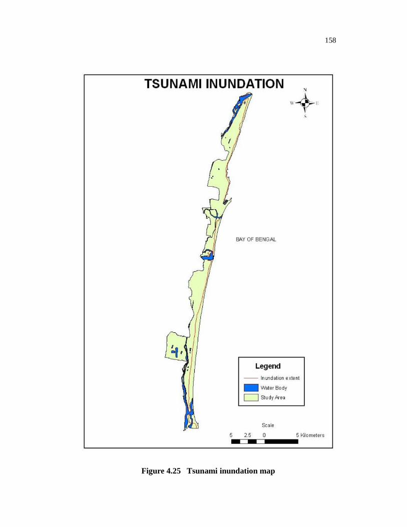
158
Figure 4.25 Tsunami inundation map
159
The presence of alternating ridges and swales also helped in modifying the
inundation as the advancing water mass after overtopping the first ridge
flowed along the intervening swale with force. Such geomorphic set up has
been observed in Kanchipuram district from Thiruvanmiyur to
Mamallapuram. This prevented reducing the distance of inundation but still
the damages were seen where structures were located in the swale area.
The creeks and the river systems having direct easterly opening to
the sea act as a carriers and carry the tsunami waves far inside on to the land.
The Ennore and Kovalam creeks have acted as carriers of tsunami waves due
to their lineament and fault controlled nature, which have aided the free flow
of tsunami waves on to the land. The construction of groynes and protection
of shore with rubble packing has saved many villages from the Tsunami
waves.
4.5.4 Coastal Erosion
The maximum rate of erosion along Tamil Nadu coast is about
6.6 m/yr near Royapuram, between Chennai and Ennore port. Thiruvottiyur is
exposed to large sea erosion due to tidal waves during monsoon. The net rate
of littoral drift or transport gives the total volume of sediment moved in a
particular direction over a year. Northerly and southerly components of
annual sediment transport along the Chennai coast is 0.89 and 0.60 106 m3
respectively. This results in a net northerly drift of about 0.30
106 m3 / annum (Mani 2001).
The Chennai coastline experiences a sediment transport of the order
of 1.6 million m3 per year towards north and 0.6 million m3 per year towards
south resulting in a net sediment transport of 1 million m3 per year towards
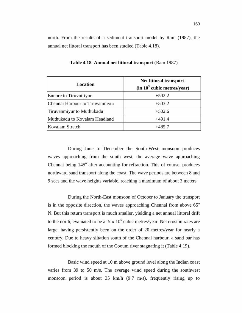
160
north. From the results of a sediment transport model by Ram (1987), the
annual net littoral transport has been studied (Table 4.18).
Table 4.18 Annual net littoral transport (Ram 1987)
Location Net littoral transport
(in 103 cubic metres/year) Ennore to Tiruvottiyur +502.2 Chennai Harbour to Tiruvanmiyur +503.2 Tiruvanmiyur to Muthukadu +502.6 Muthukadu to Kovalam Headland +491.4 Kovalam Stretch +485.7
During June to December the South-West monsoon produces
waves approaching from the south west, the average wave approaching
Chennai being 145o after accounting for refraction. This of course, produces
northward sand transport along the coast. The wave periods are between 8 and
9 secs and the wave heights variable, reaching a maximum of about 3 meters.
During the North-East monsoon of October to January the transport
is in the opposite direction, the waves approaching Chennai from above 65o
N. But this return transport is much smaller, yielding a net annual littoral drift
to the north, evaluated to be at 5 105 cubic metres/year. Net erosion rates are
large, having persistently been on the order of 20 metres/year for nearly a
century. Due to heavy siltation south of the Chennai harbour, a sand bar has
formed blocking the mouth of the Cooum river stagnating it (Table 4.19).
Basic wind speed at 10 m above ground level along the Indian coast
varies from 39 to 50 m/s. The average wind speed during the southwest
monsoon period is about 35 km/h (9.7 m/s), frequently rising up to
161
45 55 km/h (12.5 15.3 m/s). The average wind speed during northeast
monsoon prevails around 20 km/h (5.6 m/s). On open coasts with a smaller
tidal range, storm wave energies attacking the shoreline are concentrated
within a smaller vertical range and hence are likely to cause more rapid
erosional recession over a series of storms.
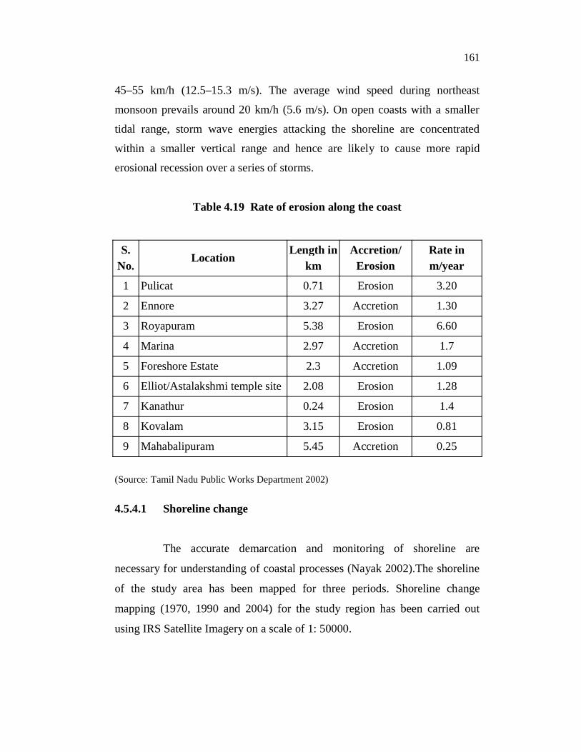
Table 4.19 Rate of erosion along the coast
S. No.
Location Length in
km Accretion/
Erosion Rate in m/year
1 Pulicat 0.71 Erosion 3.20
2 Ennore 3.27 Accretion 1.30
3 Royapuram 5.38 Erosion 6.60
4 Marina 2.97 Accretion 1.7
5 Foreshore Estate 2.3 Accretion 1.09
6 Elliot/Astalakshmi temple site 2.08 Erosion 1.28
7 Kanathur 0.24 Erosion 1.4
8 Kovalam 3.15 Erosion 0.81
9 Mahabalipuram 5.45 Accretion 0.25 (Source: Tamil Nadu Public Works Department 2002)
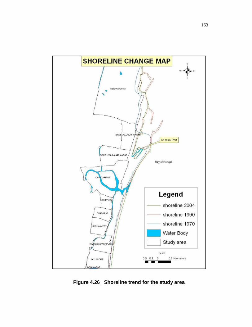
4.5.4.1 Shoreline change
The accurate demarcation and monitoring of shoreline are
necessary for understanding of coastal processes (Nayak 2002).The shoreline
of the study area has been mapped for three periods. Shoreline change
mapping (1970, 1990 and 2004) for the study region has been carried out
using IRS Satellite Imagery on a scale of 1: 50000.
162
The shoreline during the period 1970-71 has been digitized from
SOI toposheets in the scale of 1:50,000. The study region falls in three
toposheets. The toposheets numbering 66 C-7, 66 C-8 and 66 D-1&5 have
been used for the study. The three coastlines including some major features
like rivers and canal have been digitized manually from the toposheets and
three hardcopy maps obtained respectively for the three toposheets.
The shoreline of the study area during 1990 has been mapped
manually from hard copy satellite imagery. The imagery details are IRS-1A of
1990 with path 23 and row 59, in the scale of 1:50000. These maps have been
prepared by the joint efforts of the Institute of Remote Sensing, Anna
University and the Space Applications Centre, Ahmedabad under the project
The three maps comprising the study area have been scanned using
a high resolution drum scanner. The scanned sheets have been georeferenced
and transformed to the Transverse Mercator projection system. The shorelines
have been digitized from the scanned sheets using ArcGIS software. The three
shorelines from the respective maps have been combined to obtain the
complete shoreline profile of the coast from Kattivakkam to Kovalam.
The shoreline of 2004 has been geenrated from IRS-1C LISS III +
IRS-P6 merged satellite imagery of 2004 in the scale of 1:50000. An
unsupervised classification procedure using the Isodata algorithm has been
adopted to demarcate the land-water boundary in ERDAS Imagine software.
This boundary has been digitized in vector format using ArcGIS. The
generated shoreline profiles have been overlayed in GIS environment (Figure
4.26). The accretion and erosion areas have been demarcated from the map.
163
Figure 4.26 Shoreline trend for the study area
164
4.5.5 Sea-Level Rise
One of the immediate responses of ocean warming is Sea-level rise.
India has been identified as one amongst 27 countries which are most
vulnerable to the impacts of global warming related accelerated sea level rise
(UNEP 1989). Satellite altimeter observations show that global sea level has
been rising over the past decade at a rate of about 3 mm/yr, well above the
centennial rate of 1.8 mm/yr (Miller and Douglas 2001). Past observations on
the mean sea level along the Indian coast indicate a long-term rising trend of
about 1.0 mm year-1 on an annual mean basis. The corresponding thermal
expansion related sea level rise is expected to have a value of 15 to 38 cm by
the middle of the 21st century and 46 to 59 cm by the end of the century
(Aggarwal and Lal 2004).
According to TERI (1996) report, the potential impact of one metre
sea level rise on coastal land uses for Tamil Nadu, fraction of land likely to be
affected is given as: Cultivated land 0.39, Cultivable land 0.39, Forest
0.00, and Land not available for agriculture 0.21. The North Indian ocean
sea level anomaly showed a linear increasing trend of 0.31 mm/yr during
1958 2000 from a study by Thompson et al (2008). The study has been
conducted by using the Modular Ocean Model version 4.
In the coastal regions of Tamil Nadu, salinity of groundwater due to
the intrusion of seawater into the subsurface aquifer is a major problem
(Subramanian 2000). Due to excess withdrawal of groundwater, the water
table has fallen too far below thereby allowing seawater to percolate. Even
though the Intergovernmental Panel on Climate Change (IPCC) has predicted
a global sea level rise between 0.09 and 0.88 m, with a central figure of 0.48
m, by the year 2100, regional variations differ from the values due to non-
uniform patterns of temperature and salinity changes in the ocean, which, in
165
atmosphere, and on ocean transport mechanisms. Tide gauge data analysis by
Emery and Aubrey (1989) concluded that Chennai showed a sea level rise of
0.36mm/year during 1916-1977.
Using the available models, global sea-level rise of 10-25 cm per
100 years has been predicted due to the emission of GHGs. To separate the
influences due to the global climatic changes the available mean sea-level
historical data from 1920 to 1999 at 10 locations have been evaluated. The
values for Chennai indicate sea-level variations per year as -0.36 mm/year. A
minus figure indicates a relative increase in the mean sea level with respect to
the land (NATCOM 2004).
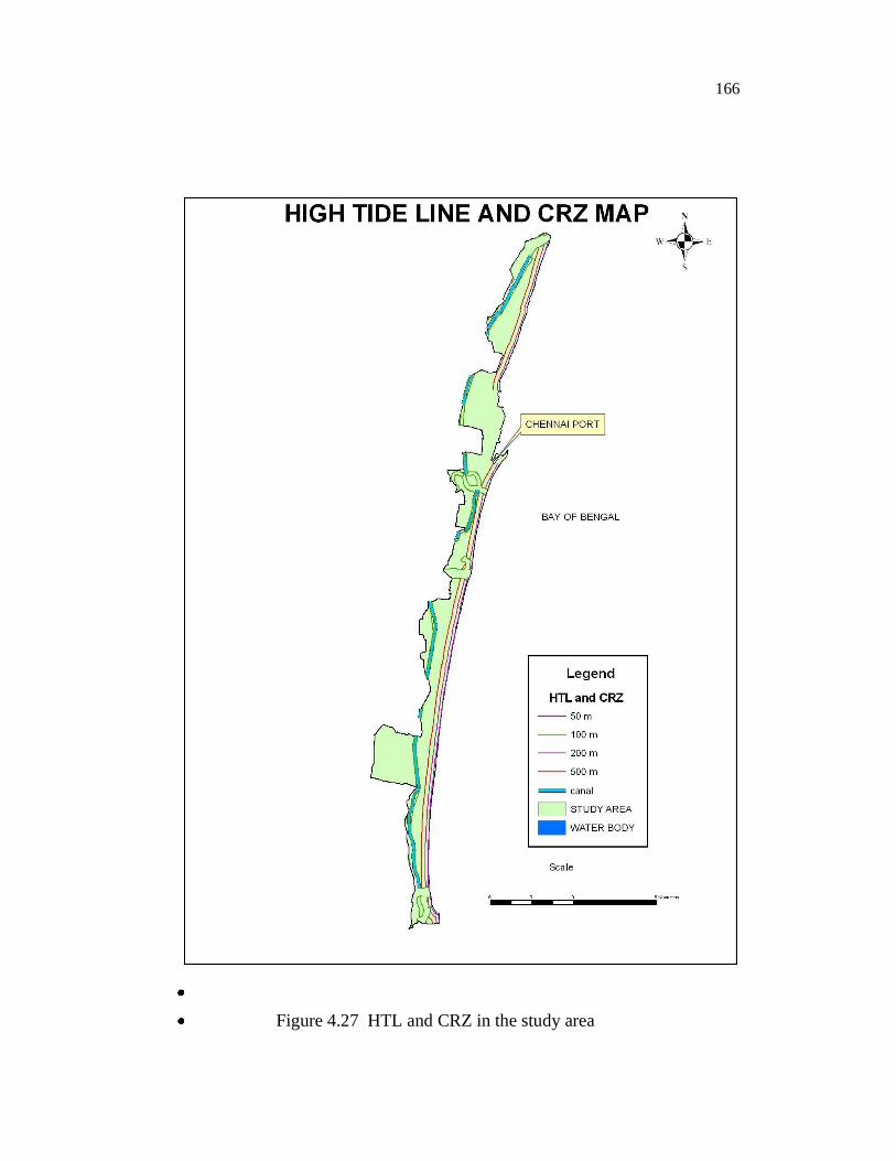
4.6 HIGH TIDE LINE AND CRZ MAP
According to the Coastal Zone regulation notification of 1991, in
India, coastal stretches of bays, estuaries, backwaters, seas and creeks which
are influenced by tidal action upto 500 m from High tide line (HTL) and
intertidal area as well as 100-150 m or width of the tidal water bodies
(whichever is less) and the land between the Low Tide line (LTL) and the
HTL has been declared as the Coastal Regulation Zone (CRZ) (Nayak 2002).
For regulating developmental activities, the coastal stretches within 500 m of
HTL of the landward side have been classifies into CRZ-I, CRZ-II, CRZ-III
and CRZ-
influence over a substantial period along the study area has been mapped
(Data courtesy: Institute of Remote Sensing, Anna University). The HTL has
been mapped by the Institute of Remote Sensing, Anna University with data
collected for maximum tidal inundation points for a considerable time period
(Figure 4.27).
166
Figure 4.27 HTL and CRZ in the study area
167
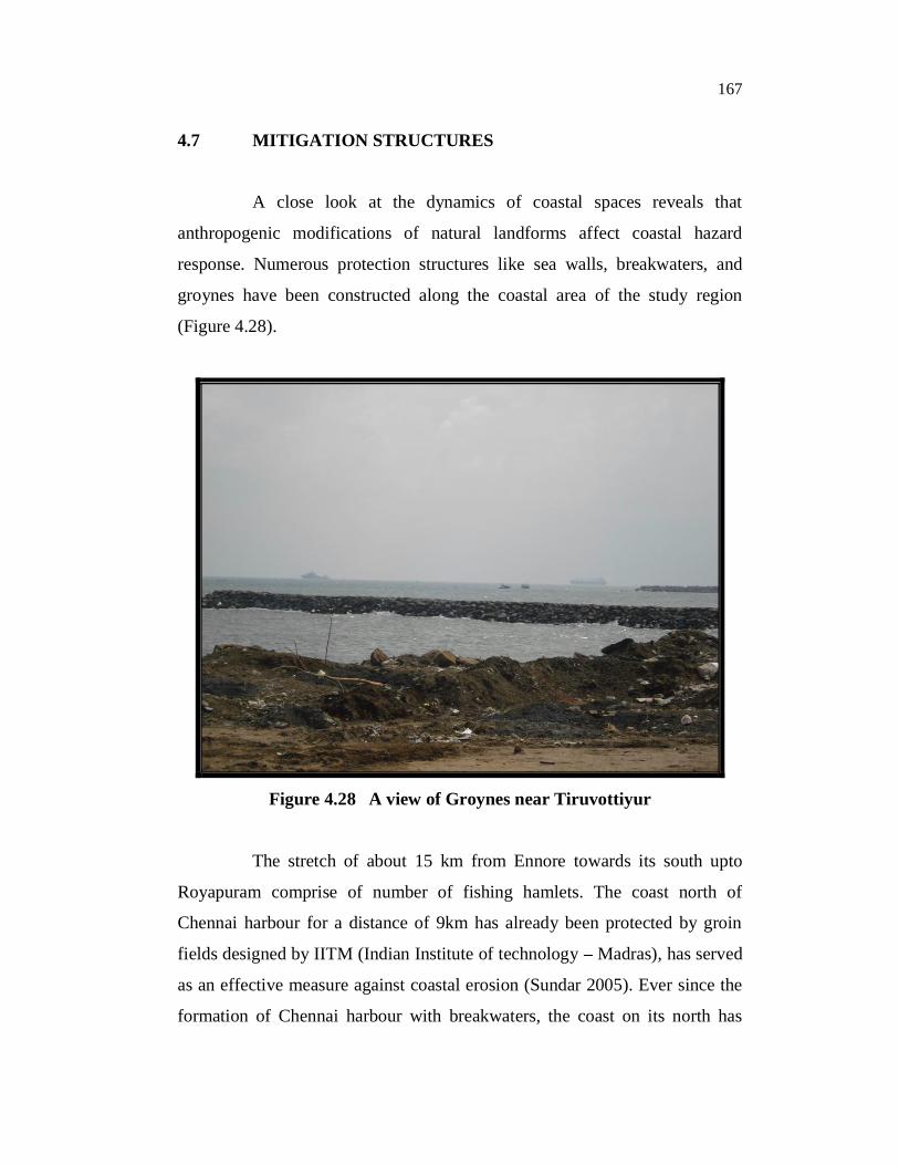
4.7 MITIGATION STRUCTURES
A close look at the dynamics of coastal spaces reveals that
anthropogenic modifications of natural landforms affect coastal hazard
response. Numerous protection structures like sea walls, breakwaters, and
groynes have been constructed along the coastal area of the study region
(Figure 4.28).
Figure 4.28 A view of Groynes near Tiruvottiyur
The stretch of about 15 km from Ennore towards its south upto
Royapuram comprise of number of fishing hamlets. The coast north of
Chennai harbour for a distance of 9km has already been protected by groin
fields designed by IITM (Indian Institute of technology Madras), has served
as an effective measure against coastal erosion (Sundar 2005). Ever since the
formation of Chennai harbour with breakwaters, the coast on its north has
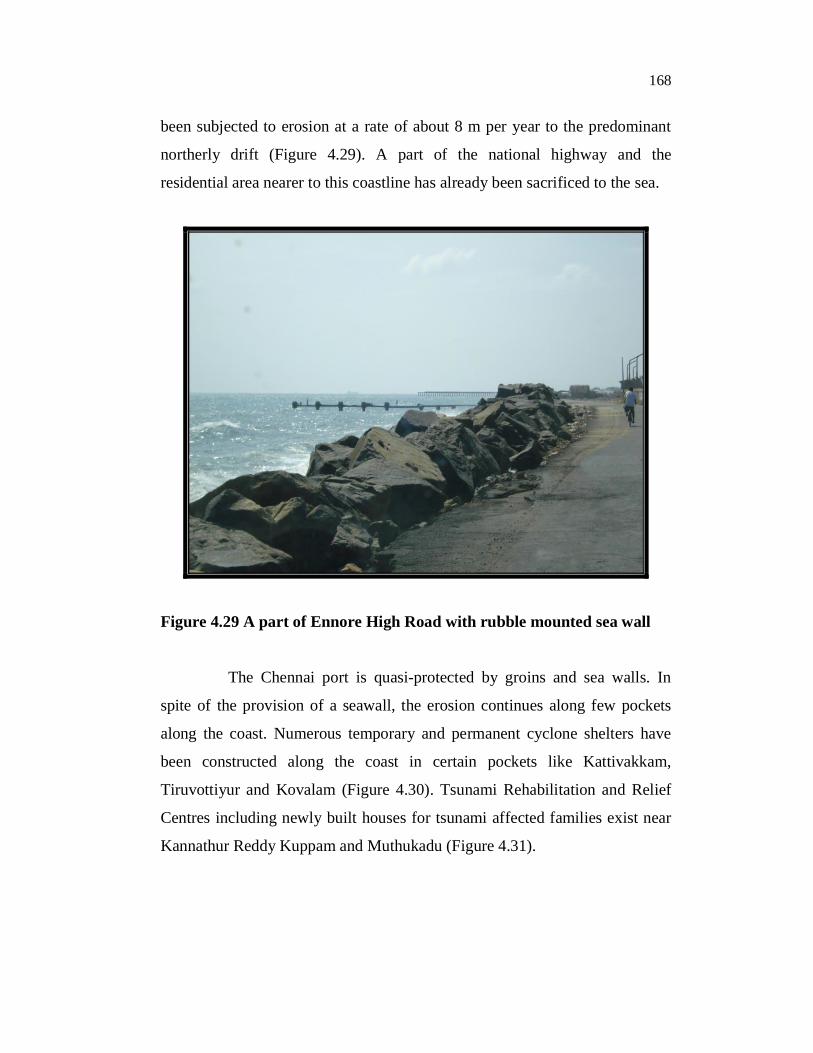
168
been subjected to erosion at a rate of about 8 m per year to the predominant
northerly drift (Figure 4.29). A part of the national highway and the
residential area nearer to this coastline has already been sacrificed to the sea.
Figure 4.29 A part of Ennore High Road with rubble mounted sea wall
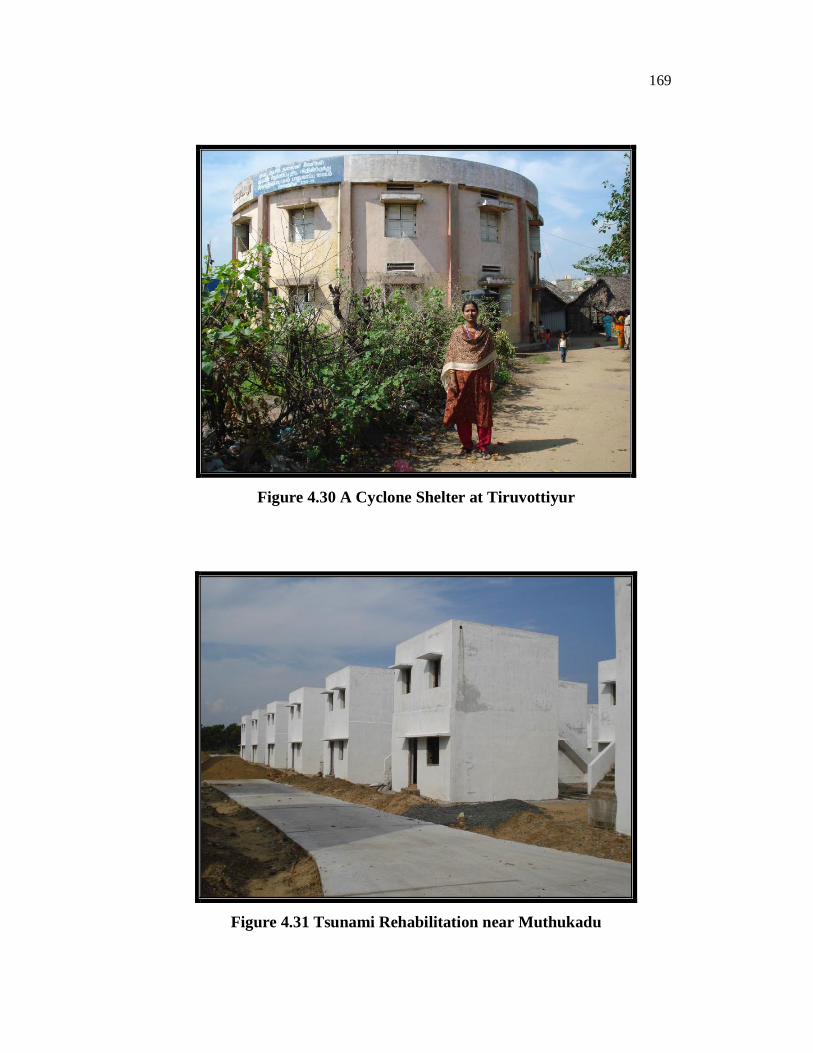
The Chennai port is quasi-protected by groins and sea walls. In
spite of the provision of a seawall, the erosion continues along few pockets
along the coast. Numerous temporary and permanent cyclone shelters have
been constructed along the coast in certain pockets like Kattivakkam,
Tiruvottiyur and Kovalam (Figure 4.30). Tsunami Rehabilitation and Relief
Centres including newly built houses for tsunami affected families exist near
Kannathur Reddy Kuppam and Muthukadu (Figure 4.31).
169
Figure 4.30 A Cyclone Shelter at Tiruvottiyur
Figure 4.31 Tsunami Rehabilitation near Muthukadu