Finding Optimal Reduct for Rough Sets by Using a Decision

San Jose State University San Jose State University

SJSU ScholarWorks SJSU ScholarWorks

Master's Projects Master's Theses and Graduate Research

2006

Finding Optimal Reduct for Rough Sets by Using a Decision Tree Finding Optimal Reduct for Rough Sets by Using a Decision Tree

Learning Algorithm Learning Algorithm

Xin Li San Jose State University

Follow this and additional works at: https://scholarworks.sjsu.edu/etd_projects

Part of the Computer Sciences Commons

Recommended Citation Recommended Citation Li, Xin, "Finding Optimal Reduct for Rough Sets by Using a Decision Tree Learning Algorithm" (2006). Master's Projects. 125. DOI: https://doi.org/10.31979/etd.nuhk-2kpp https://scholarworks.sjsu.edu/etd_projects/125

This Master's Project is brought to you for free and open access by the Master's Theses and Graduate Research at SJSU ScholarWorks. It has been accepted for inclusion in Master's Projects by an authorized administrator of SJSU ScholarWorks. For more information, please contact [email protected].

https://scholarworks.sjsu.edu/

https://scholarworks.sjsu.edu/etd_projects

https://scholarworks.sjsu.edu/etd

https://scholarworks.sjsu.edu/etd_projects?utm_source=scholarworks.sjsu.edu%2Fetd_projects%2F125&utm_medium=PDF&utm_campaign=PDFCoverPages

http://network.bepress.com/hgg/discipline/142?utm_source=scholarworks.sjsu.edu%2Fetd_projects%2F125&utm_medium=PDF&utm_campaign=PDFCoverPages

https://scholarworks.sjsu.edu/etd_projects/125?utm_source=scholarworks.sjsu.edu%2Fetd_projects%2F125&utm_medium=PDF&utm_campaign=PDFCoverPages

mailto:[email protected]

Finding Optimal Reduct for Rough Sets by Using a Decision Tree Learning Algorithm

A Project Report

Presented to

The Faculty of the Department of Computer Science

San Jose State University

by

Xin Li

May 2006

[email protected]

Advisor: Dr. T.Y. Lin

[email protected]

mailto:[email protected]

AbstractRough Set theory is a mathematical theory for classification based on structural

analysis of relational data. It can be used to find the minimal reduct. Minimal reduct is

the minimal knowledge representation for the relational data. The theory has been

successfully applied to various domains in data mining. However, a major limitation in

Rough Set theory is that finding the minimal reduct is an NP-hard problem. C4.5 is a

very popular decision tree-learning algorithm. It is very efficient at generating a decision

tree. This project uses the decision tree generated by C4.5 to find the optimal reduct for

a relational table. This method does not guarantee finding a minimal reduct, but test

results show that the optimal reduct generated by this approach is equivalent or very

close to the minimal reduct.

2

Table of contents

Abstract.............................................................................................................................................................21 Introduction....................................................................................................................................................42 Rough Sets and Relational Table...................................................................................................................7

2.1 Preliminaries....................................................................................................................................... 73 C4.5..............................................................................................................................................................13

3.1 Preliminaries..................................................................................................................................... 153.2 Example............................................................................................................................................ 17

4 Finding Minimal Rules................................................................................................................................ 254.1 Feature selection............................................................................................................................... 294.2 user input, randomize attribute selection and best attribute selection.............................................. 41

4.2.1 Randomize attribute selection....................................................................................................444.2.2 Best Attribute selection..............................................................................................................464.2.3 User input...................................................................................................................................50

Figure 4-5................................................................................................................................................514.3 Finding the decision rules.................................................................................................................514.4 Using threshold to generate the rules................................................................................................55

5 Result comparison....................................................................................................................................... 576 Conclusion................................................................................................................................................... 62References.......................................................................................................................................................63Appendix A – Source code for this project ................................................................................................... 65Appendix B – Data set of Monk3 Sample.................................................................................................... 124

3

1 Introduction

Data mining can be defined as “The nontrivial extraction of implicit, previously

unknown, and potentially useful information from data” (Frawley et al. 1992). Data

mining is used by all sorts of organizations and businesses to identify trends across large

sets of data. Once these patterns are identified they can be used to enhance decision

making in a number of areas.

Data mining is quite pervasive in today’s society and greatly affects the way we

are marketed to by corporate America. Advertisers and marketers depend so heavily on

data mining and the trend analysis that it provides, that it is hard to imagine life without

it. The information harnessed via data mining techniques govern our buying patterns, the

food we eat, the medicine we take and so many other facets of our daily lives. For

example, one large North American chain of supermarkets discovered through the mining

of their data that beer and diapers were often sold together. They used this information to

strategically place the two items in close proximity to one another within their stores and

saw sales of both climb. Without mining data the greatest of marketers would have had a

tough time discovering such a correlation. Another and perhaps more practical

application comes from the medical field. Historical patient data is often mined in

conjunction with disease information to determine correlations between demonstrated

symptoms and disease. Such applications of data mining are able to diagnose and treat

4

diseases earlier. It is these sorts of applications that make data mining so important to

our society today.

Rough Set theory as introduced by Zdzislaw Pawlak in 1982 can be used to create

a framework for data mining. Rough Set theory provides many good features, such as

representing knowledge as an equivalence class, generating rules from a relational data

table and finding the minimal reduct from a relational data table. Rough Set theory is an

elegant theory when applied to small data sets because it can always find the minimal

reduct and generate minimal rule sets. However, according to (Komorowski et al, 1998),

the general solution for finding the minimal reduct is NP-hard. An NP-hard problem is

defined a problem that cannot be solved in polynomial time. In other words as data sets

grow large in both dimension and volume, finding the minimal reduct becomes

computationally impossible.

The C4.5 algorithm is an extension of ID3 algorithm, a classification algorithm

used to generate decision trees. C4.5 enhanced ID3 by better attribute selection method,

handling missing values, continuous attributes. The C4.5 tree-induction algorithm is

capable of generating small decision trees quite quickly. However, it is not necessarily

the best solution, as it does not always generate the smallest decision tree possible. In

cases where multiple attributes have the same gain ratio, C4.5 is not guaranteed to choose

the attribute that will generate the smallest sub-tree. By failing to choose the best attribute

to build the decision tree, C4.5 leaves room for improvement.

In our project we sought to improve upon the C4.5 algorithm by applying the

Greedy Algorithm to attributes with the same gain ratio. By applying the Greedy

5

Algorithm we are always able to generate equal or smaller decision trees given the same

data set when compared to the original C4.5 algorithm. By combining Rough Set theory

and the output decision trees of our modified C4.5 algorithm we are able to find the

Optimal Reduct.

The advantage of this algorithm is that finding the Optimal Reduct unlike the

minimal reduct is not an NP-Hard problem. Therefore generating the optimal rule set for

large data sets become computationally possible using our algorithm. Our results prove

that generating the Optimal Reduct is exponentially more attainable than the minimal

reduct given the same computing resources. Our tests also show that the Optimal Reduct

only slightly increases the total number of rules as compared with the minimal reduct.

Given these two findings, the Optimal Reduct is a practical solution given the NP-hard

problem faced by Rough Set theory when dealing with large data sets.

6

2 Rough Sets and Relational Table

Rough Set theory is a popular theory in data mining (Pawlak, 1982). Unlike the

traditional database, which focuses on storing and retrieving data, Rough Set theory focus

on analyzing and finding the useful trends, patterns and information from the data. The

main techniques are set approximation and the reduct generation. The following

introduces the definitions and concepts of Rough Set theory.

2.1 Preliminaries

Definition 2.1: Decision System

A Decision System can be described as DS=(U, A), where U is a nonempty finite set of

objects and A is a nonempty finite set of attributes. The elements is called objects. For

every a∈A, aV is the allowed attribute values.

The following demonstrates a decision system via a simple hiring example.

Suppose a department in a company needs to hire some people. A criterion is used to

select the candidates for onsite interviews. There are eight total candidates and they are to

be evaluated on four different sets of attributes (Education Level, Years of Experience,

Oracle technology, Java technology). The criterion has one decision attribute, On-site

interview. The rows represent objects or people in this case, and the columns represent

attribute value pairs for each of the objects.

Candidates Education Experience Oracle technology (For example: ADF)

Java technology

On-site interview

7

Candidate 1 Bachelor Senior (> 3 years)

Yes Yes Yes

Candidate 2 High School

Senior (> 3 years)

Yes Yes Yes


Junior No Yes No

Candidate 4 Ph.D. Junior Yes Yes Yes

Candidate 5 Bachelor Junior Yes Yes Yes

Candidate 6 Master Senior (> 3 years)

No Yes Yes


Junior Yes Yes No


No No No

Table 2-1

Definition 2.2: Equivalence Class

Let x, y and z be the objects in U. if xRx=xRx, xRy=yRx and xRy, yRz, then xRz, we call

R the equivalence Relation. The equivalence class is a subset of U, and all the elements

in the equivalence class have the equivalence relation with each other.

Definition 2.3: Indiscernibility Relation

The indiscernibility relation IND(P) is a equivalence relation. With every subset of

attributes P ⊆ A in decision system the indiscernibility relation can be defined as follows

IND(P)={(x,y)∈U×U, for every a ∈ P, a(x)=a(y)}

8

Elementary set, U/IND(P), means the set of all the equivalence classes in the relation

IND(P)

For the decision system given in the Table 2-1, U/IND(P) gives the following

result:

U/IND({Education})={ {C1, C5, C8}, {C2, C3 C7}, {C4}, {C6}}

U/IND({Experience})={ {C1, C2, C6, C8}, {C3, C4, C5, C7}}

U/IND({Education, Experience})={{C1, C8}, {C2}, {C3, C7}, {C4}, {C5}, {C6}}

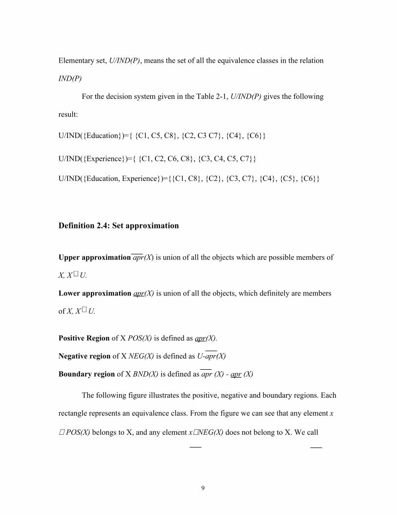
Definition 2.4: Set approximation

Upper approximation apr(X) is union of all the objects which are possible members of

X, X ⊆ U.

Lower approximation apr(X) is union of all the objects, which definitely are members

of X, X ⊆ U.

Positive Region of X POS(X) is defined as apr(X).

Negative region of X NEG(X) is defined as U-apr(X)

Boundary region of X BND(X) is defined as apr (X) - apr (X)

The following figure illustrates the positive, negative and boundary regions. Each

rectangle represents an equivalence class. From the figure we can see that any element x

∈ POS(X) belongs to X, and any element x∈NEG(X) does not belong to X. We call

9

POS(X) ∪BND(X) upper approximation apr(X) of a set X. For any element x∈ apr(X) ,

it possible belongs to X.

Figure 2-1

Positive Region

Boundary Region

Negative Region

Rough Set theory is the study of the boundary region. The following are properties of the

approximation sets:

1. apr(X) ⊃ X ⊃ apr(X)

10

2. apr(U) = apr(U) = U, apr(∅) = apr(∅) = ∅

3. apr(X ∪ Y) = apr( X ) ∪ apr ( Y )

4. apr(X ∩ Y) = apr( X ) ∩ apr ( Y )

5. apr(X ) = - apr( U- X )

6. apr(X ) = - apr( U- X )

7. apr(X ∩ Y) ⊂ apr( X ) ∩ apr ( Y )

8. apr(X ∪ Y) ⊃ apr( X ) ∪ apr ( Y )

9. apr(X - Y) ⊃ apr( X ) - apr ( Y )

10. apr(X - Y) ⊂ apr( X ) - apr ( Y )

11. X ⊂ Y → apr( X ) ⊂ apr ( Y)

12. X ⊂ Y → apr( X ) ⊂ apr ( Y)

13. apr( X ) ∪ apr (-X ) = -BND( X )

14. apr( X ) ∩ apr ( Y ) = BND( X )

For the decision system given in the Table 2-1, when just using the attribute

“Education” to classify the decision system, for the “Yes” decision, X={C1, C2, C4, C5,

C6}.

U/IND({Education})={ {C1, C5, C8}, {C2, C3 C7}, {C4}, {C6}}

Apr(X)= {C4, C6}

11

Apr(X)={C1, C2, C3, C4, C5, C6, C7, C8}

}{educationPOS (X) = apr(X) = {C4, C6}

}{educationNEG (X) = U- apr(X) = ∅

}{educationBND (X) = apr(X)-apr(X) = {C1, C2, C3, C5, C7, C8}

Decision rules we can derive:

If Education = Ph.D or Education = Master

--> Have on-site interview

If Education = Bachelor or Education = High School

--> Unknown

Definition 2.5: Dispensable and Indispensable attributes

An attribute a is dispensable in P if POS(P)=POS(P-{a}), otherwise the attribute a is

indispensable attribute in P.

For the decision system given in the Table 2-1, when P={Education, Experience,

Oracle technology, Java technology}, for “Yes” decision, },,,{ JavaOracleExperienceEducationPOS

({C1, C2, C4, C5, C6}) = },{ JavaExperienceEducationPOS ({C1, C2, C4, C5, C6}). For “No”

decision, },,,{ JavaOracleExperienceEducationPOS ({C3, C7, C8})= },{ JavaExperienceEducationPOS ({C3, C7,

C8})

12

In this case the attribute Oracle technology is a dispensable attribute.

Definition 2.6: Reduct

The reduct is a minimal subset of attributes A, which classify the universe U into the

same set of the equivalence class. For a given attribute set A, the reduct is not unique.

For the previous example in Table 2.1, the reduct could be:

{Education, Experience, Oracle technology} or {Education, Experience, Java

technology}

Definition 2.7: Decision rules

With every object in the universe U we associate a function xD : A →V, the function xD

is a decision rule. A represents attributes, and V represents decision value. The minimal

decision rules are the minimal set of rules that classify the universe U into the same set of

the equivalence class.

3 C4.5

C4.5 algorithm is based on ID3 algorithm. They are both introduced by Quinlan, J. Ross

to generate the decision trees from data (Quinlan, 1993). C4.5 improves on ID3 by using

the gain ratio criterion instead of the gain criterion to select an attribute. C4.5 can handle

missing values, continuous attribute value ranges and prune the decision trees. A decision

tree can be used to sort down a tree from the root to the leaf to classify the instances.

13

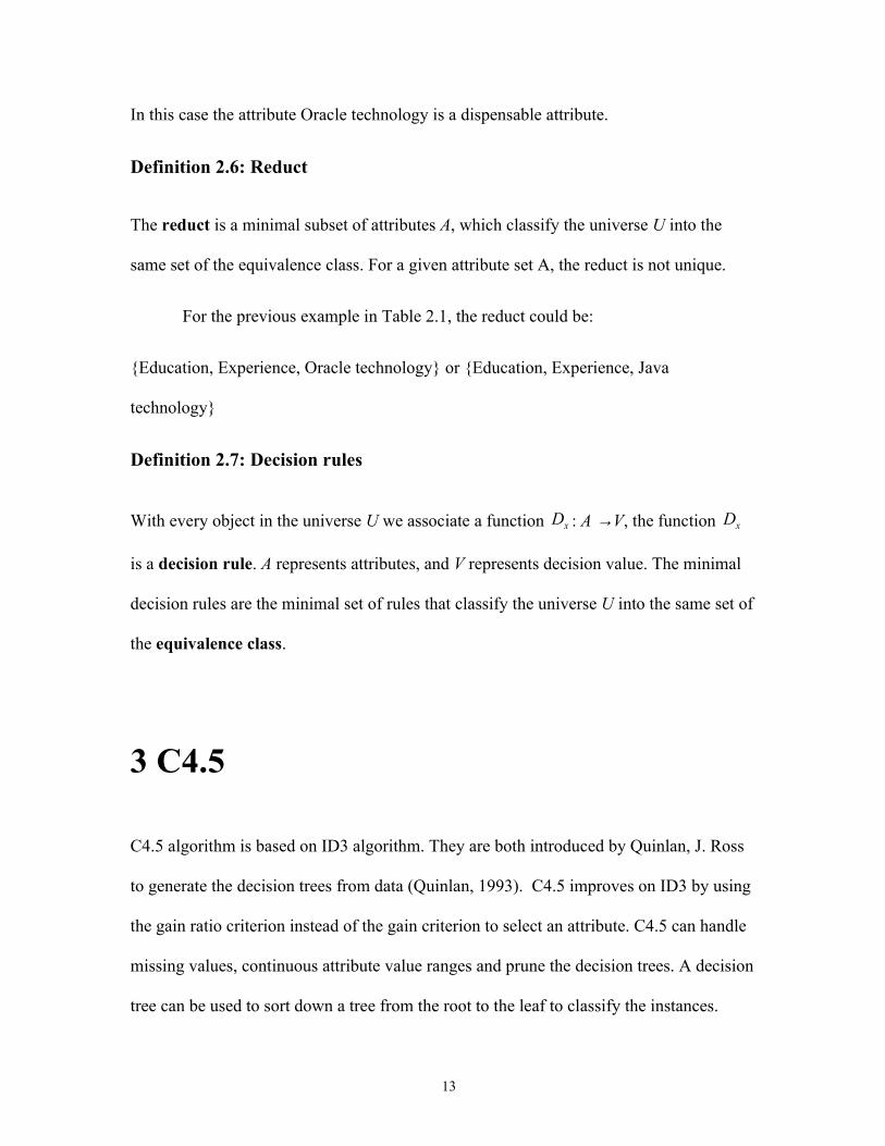
Each node in the tree represents a condition attribute in the decision system. Each leaf

represents a decision value in the decision system. For example,

Figure 3-1: Decision Tree for Golf Data

14

From this decision tree, golf is played when the outlook is sunny and humidity is

equal to or less than 75 degrees. When the outlook is sunny and humidity is greater than

75 degrees, a decision is made not to play golf. When outlook is overcast golf is played.

When outlook is rainy and windy golf is not played. Finally, when outlook is rainy and

not windy golf is played.

Not all the classification tasks can use C4.5. There are several prerequisites:

• All the data can be described as attribute-value table. This table has fixed

collection of properties or attributes.

• The table has predefined classes.

• The class type is discrete.

We have sufficient data.

3.1 Preliminaries

As described in (Quinlan, 1993), if there are n equally probable possible

messages, the probability of each message is 1/n. The information conveyed by any one

of the messages is )1(log2 n− . For example: if there are 8 messages, then 3)

81(log2 =− .

So we need 3 bits to identify each message. If there is a set of cases S and it has

),...,,( 21 kCCC classes, then ),( SCfreq j means the number of cases in S that belongs to

jC and S means the number of cases in the set S. Selecting any case randomly from S

15

that is in jC has probability SSCfreq j ),(

and the information conveyed by this is

)),(

(log2 SSCfreq j− bits. The average amount of information we need to identify the

class of a case in T is ∑=

×−=k

j

j

SSCfreq

SSCjfreqSInfo

12 )

),((log),()(

If we partition T on the basis of the value of test X into sets nTTT ,..., 21 then the

information needed to identify the class of a case of T becomes the weighted average of

the information needed to identify the class of a test of Ti

∑=

×=n

in

nx TInfo

TT

TInfo1

)()(

Consider the quantity Gain(X) defined as

)()()( TInfoTInfoXGain x−=

This represents the difference between the information needed to identify a case

of T and the information needed to identify a case of T after the value of test X has been

obtained; that is, this is the gain information due to test X.

The gain gave very good results but it has a strong bias to the attribute that has

the most different values. From the prediction point of view, to choose this kind of the

16

attribute is useless. For example, most database tables have the primary key. In these

tables, by using the gain, it would like to select the primary key. The primary key is not

very helpful for finding the knowledge in data mining. In C4.5, Quinlan suggests to use

Gain Ratio.

We can use gain ratio to choose the attribute that has the greatest gain among all

attributes and then use this attribute as one node of the tree. By doing this we are able to

create a small decision tree.

)()()(

XsplitXGainXGainRatio =

∑=

×−=n

i

ii

TT

TT

XSplit1

2 )(log)(

Where ),...,( 21 nTTT is the partition of T induced by the value of X.

3.2 Example

Table 2-1 hiring example is used again to illustrate the C4.5 algorithm.

Candidates Education Experience Oracle technology (For example:

C4.5)

Java technology

On-site interview


Yes Yes Yes

17


Senior (> 3 years)

Yes Yes Yes


Junior No Yes No

Candidate 4 Ph.D. Junior Yes Yes Yes

Candidate 5 Bachelor Junior Yes Yes Yes

Candidate 6 Master Senior (> 3 years)

No Yes Yes


Junior Yes Yes No


No No No

In the table, the columns of the table are named attributes. The first four columns

are further defined as conditional attributes. The last column is referred to as the decision

attribute. The rows of the table are referred to as objects. The entries in the table are

called attribute-values. Then each row of the table can be seen as the information for a

particular candidate. From the data in this table we can determine that if a candidate

demonstrates an education level of Masters or Ph.D degree then said candidate will be

rewarded an on-site interview. The decision tree would appear as follows:

Education = Bachelor:

| Experience = Senior:

18

| | Oracle Technology = Yes: Yes

| | Oracle Technology = No: No

| Experience = Junior: Yes

Education = High School:

| Experience = Senior: Yes

| Experience = Junior: No

Education = Master: Yes

Education = Ph.D: Yes

Tree 1

In this decision tree, the first attribute is chosen to divide the objects and then

second and third attributes are selected until a decision is made whether or not to bring

the candidate in for an on-site interview.

When using C4.5, it tries to choose the attribute that generates a small decision

tree. The following demonstrates the C4.5 algorithm. There are two classes (Yes and No

for On-Site interview), five objects belong to Yes and three objects belong to No.

954.0)83(log

83)

85(log

85)( 22 =×−×−=TInfo

This represents the average information needed to identify the class of the case in

T. After using the “Education” to divide T into four subsets, the result is 0.687

))31(log

31)

32(log

32(

83))

32(log

32)

31(log

31(

83)( 2222 ×−×−×+×−×−×=TInfox

687.0))11(log

11(

81))

11(log

11(

81

22 =×−×+×−×+

19

The information gained by this test is 0.266.

266.0686.0954.0)()()( =−=−= TInfoTInfoXGain x

811.1)81(log

81)

81(log

81)

83(log

83)

83(log

83)( 2222 =×−×−×−×−=XSplit

147.0811.1266.0

)()()( ===

XSplitXGainXGainRatio

Now suppose that, instead of dividing T on the attribute “Education”, we have

partitioned it on the attribute “Experience”. After using “Experience” to divide T into two

subsets, the similar computation is shown below.

906.0))42(log

42)

42(log

42(

84))

41(log

41)

43(log

43(

84)( 2222 =×−×−×+×−×−×=TInfox

048.0906.0954.0)(inf)(inf)( =−=−= ToToXGain x

1)84(log

84)

84(log

84)( 22 =×−×−=XSplit

048.01048.0

)()()( ===


When using “Oracle technology” to divide T, we get the following values

20

795.0))31(log

31)

32(log

32(

83))

51log(

51)

54(log

54(

85)( 222 =×−×−×+×−×−×=TInfox

159.0795.0954.0)()(inf)( =−=−= TInfoToXGain x

954.0)83(log

83)

85(log

85)( 22 =×−×−=XSplit

166.0954.0159.0

)()()( ===


When using “Java technology” to divide T, we get the following values.

755.0))11(log

11(

81))

72(log

72)

75(log

75(

87)( 222 =×−×+×−×−×=TInfox

199.0755.0954.0)()(inf)( =−=−= TInfoToXGain x

544.0)81(log

81)

87(log

87)( 22 =×−×−=XSplit

365.0544.0199.0

)()()( ===


Based on the calculation, C4.5 chooses “Java Technology” to divide the T first,

and the tree becomes:

21

Java Technology = Yes:

Java Technology = No: No

After using the Java Technology to divide the tree the table looks as follow:

When Java Technology = yes

Candidates Education Experience Oracle Technology On-site interview

1 Bachelor Senior Yes Yes

2 High School Senior Yes Yes

3 High School Junior No No

4 PH.D. Junior Yes Yes

5 Bachelor Junior Yes Yes

6 Master Senior No Yes

7 High School Junior Yes No

Table 3-1

When Java Technology = no

Candidates Education Experience Oracle Technology On-site interview

8 Bachelor Senior No No

Table 3-2

The same method is recursively used to calculate the Gain Ratio for each

attributes in Table 3-1 and Table 3-2. Finally we get the following decision tree.

Java = No: No (1.0)

22

Java = Yes:

| Experience = Senior: Yes

| Experience = Junior:

| | Education = Bachelor: Yes

| | Education = High School: No

| | Education = PH.D.: Yes

| | Education = Master: Yes

Tree 2

When running the above example through the C4.5 program, we can see the

following output.

Figure 3-2

By comparing Tree 1 and Tree 2, we can see that for Tree 1, we manually pick the

attribute. In this case we pick the attribute from left to right in the columns. So it picks

“Education” to start creating the tree. C4.5 picks “Java Technology” to start creating the

tree. We can tell that the tree created by C4.5 has smaller size than the manual process.

23

By testing C4.5 on other data sets, we see that C4.5 generates smaller decision trees and

is very fast.

24

4 Finding Minimal RulesDecision rules finding, especially optimal decision rules finding is a crucial task in Rough

Set applications. The purpose of this project is to generate the optimal decision rule for

Rough Set by using the C4.5 algorithm. Though this method does not guarantee finding

the minimal set of rules, it does often find the minimal set. In the cases where it does not

find the minimal set it does find sets that number very close to the minimum.

The project is based on C4.5 and adds several options to generate an optimal

reduct. The program workflow is shown below:

25

26

Figure 4-1

Step One: The algorithm uses the feature selection first to remove the dispensable

attributes from the decision system. By using the feature selection, the unrelated attribute

data will not be considered when building the decision tree from C4. 5.

Step Two: The algorithm uses this modified version of C4.5 to generate the decision tree.

The C4.5 is modified to select the best node attribute when there are multiple attributes

with the same gain ratio. For those decision systems that have this specific attribute

situation, our decision tree is smaller than the tree generated by the original C4.5. By

generating a smaller decision tree we are in turn generating a smaller set of rules in the

later steps of the process.

Step Three: Convert the generated decision tree to rules format.

Step Four: Evaluate each rule to remove the superfluous attribute-values. When using

different sequence to evaluate each attribute values in the rule will generate different

subset of rules. In the algorithm, every attribute in the decision system is used as the first

attribute to evaluate the rule. After the subset of rules being generated, the algorithm

chooses the best rule whose length of the rule is the smallest. Here the length of the rule

means the number of attribute values the rule needs to classify the objects.

Step Five: Remove the duplicate rules. After the rules have been simplified, different

rules may cover the same set of objects in the decision system. This process is used to

remove the duplicate rules, leaving only the necessary rules for decision table

classification.

27

Step Six: Apply the threshold to display the decision rules. When a decision system has

hundreds of objects it may generate hundreds of decision rules. In this case, it would be

very hard for user to read all the rules. If a user specifies a threshold, the program will

just show the rules which are suitable for more objects than the threshold value. User can

base on the need to specify this value.

The following method constructs the decision tree used in modified C4.5 with a

“divide and conquer” strategy. Each node in the tree is associated with a set of cases. In

the beginning, only the root is present and associated with the whole training set. At each

node, the following “divide and conquer” algorithm is executed.

FormTree(T){

ComputeClassFrequency(T);if T belongs to OneClass{

return a leaf;}create a decision node N;ForEach( Attribute A){

ComputeGainRatio(A);}N.BestAtt=AttributeWithBestGainRatio;if ( there are multiple BestAtts){

calculate the subtree for each BestAtts;N.BestAtt=Att associated with the smallest tree size;

}Child of N = FormTree (T');return N;

}

28

For a set of data, it calculates the Class Frequency first. If the data set belongs to

one class, the algorithm returns a leaf; otherwise, it creates a decision node N. For each

attribute it calculates the Gain Ratio value. The algorithm picks the highest Gain Ratio

value attribute as the best attribute. If there are multiple attributes (say set MA) with the

same best Gain Ratio value, the algorithm will generate the sub-tree for each attribute in

MA and use the attribute that has the smallest sub-tree size as the best attribute. C4.5

will use the best attribute to divide the data set and generate the node.

4.1 Feature selection

Feature selection, also known as subset selection or variable selection, is a process

commonly used in data mining. The main idea of feature selection is to choose a subset

of the input variables by removing features with little or no predictive information.

Feature selection is necessary because sometimes there are too many features and it is

computationally infeasible to use all the available features.

In this project, we use the functional dependency concept to evaluate every

attribute to see if the attribute is dispensable and mark every attribute accordingly. (A

functional dependency is a constraint between two sets of attributes in a relation. Given a

relation R, a set of attributes X is said to functionally determine another attribute Y if and

only if each X value is associated with at most one Y value, we write as X → Y (S.

Krishna, 1992)) The algorithm removes one attribute at a time and checks if the

remaining condition attribute can determine the decision attribute. If the remaining

attributes → decision attribute, the attribute will be marked as “true”. If the remaining

attributes cannot determine decision attribute then the attribute is marked “false”. After

29

each attribute has been evaluated, C4.5 will check the mark and decide whether it needs

to calculate the gain ratio for this attribute. If the attribute is marked “true”, C4.5 will not

calculate the gain ratio for this attribute and will not use this attribute to build the tree.

The algorithm for the feature selection is shown below.

R = the set of attributes in CON;AttUse = the mark to indicate if the attribute is dispensableFeatureSelection(R){

InitAttUse(); // Set the default value to false for all the AttUse[i], means all the //attributes are indispensable.ForEach (i, 0, MaxAtt){

Boolean flag=checkAttribute(i, R); //Check if the remaining attributes can // determine the decision value.if (flag){

AttUse[i]=true; //Means the ith attribute can be cut. R=R-ith;

}}

}

Boolean checkAttribute(Att, R){

R=R-Att;If(R is consistent){

Return true;}else{

return false;}

}

The algorithm checks each attribute in sequence from the first attribute to the last

attribute in the table and determines if the attribute can be removed. This option is mainly

30

used for data sets that have many condition attributes. This helps simplify the

computation for the later stages.

The example, which follows (Pawlak, 1991), refers to an optician's decisions as to

whether or not a patient is suitable for contact lenses. The set of all possible decisions is

listed in Table 4-1.

U a b c d e f

1 1 1 2 2 1 1

2 1 2 2 2 1 1

3 2 1 2 2 1 1

4 3 1 2 2 2 1

5 1 1 1 2 1 2

6 1 2 1 2 1 2

7 2 1 1 2 1 2

8 2 2 1 2 1 2

9 3 2 1 2 2 2

10 1 1 1 1 1 3

11 1 1 2 1 1 3

12 1 2 1 1 1 3

13 1 2 2 1 1 3

14 2 1 1 1 1 3

15 2 1 2 1 1 3

31

U a b c d e f

16 2 2 1 1 1 3

17 2 2 2 1 1 3

18 2 2 2 2 1 3

19 3 1 1 1 2 3

20 3 1 1 2 2 3

21 3 1 2 1 2 3

22 3 2 1 1 2 3

23 3 2 2 1 2 3

24 3 2 2 2 2 3

Table 4-1

The table is in fact a decision table in which a, b, c, d and e are condition

attributes whereas f is a decision attribute.

The attribute f represents optician's decisions, which are the following:

1. Hard contact lenses.

2. Soft contact lenses

3. No contact lenses

These decisions are based on some facts regarding the patient, which are expressed by the

condition attributes, given below together with corresponding attribute values.

a - Age1 - young2 – pre-presbyopic

32

3 – presbyopicb – spectacle

1 – myope2 – hypermetrope

c – astigmatic1 – no2 – yes

d – tear production rate1 – reduced2 – normal

e- working environment1 – computer related2 – non-computer related

Here we need to use the feature selection to eliminate the unnecessary conditions from

a decision table.

Step1:

Removing attribute a in Table 4-1 will result in the following decision table

U a b c d e f

1 1 2 2 1 1

2 2 2 2 1 1

3 1 2 2 1 1

… … … … … …

17 2 2 1 1 3

18 2 2 2 1 3

19 1 1 1 2 3

33

U a b c d e f

… … … … … …

24 2 2 2 2 3

Table 4-2

From the Table 4-2 we see the following pairs of inconsistent decision rules

b2c2d2e1 -> f1 (row 2)b2c2d2e1 -> f3 (row 18)

This means that the conditions b,c,d and e cannot determine decision f. Thus the attribute

a cannot be dropped.

Step 2:

Similarly removing attribute b we get the following decision table.

U a b c d e f

1 1 2 2 1 1

2 1 2 2 1 1

3 2 2 2 1 1

4 3 2 2 2 1

5 1 1 2 1 2

… … … … … …

34

U a b c d e f

8 2 1 2 1 2

9 3 1 2 2 2

10 1 1 1 1 3

… … … … … …

17 2 2 1 1 3

18 2 2 2 1 3

19 3 1 1 2 3

20 3 1 2 2 3

21 3 2 1 2 3

22 3 1 1 2 3

23 3 2 1 2 3

24 3 2 2 2 3

Table 4-3

From the Table 4-3 we the following pairs of inconsistent decision rules can be seen

a2c2d2e1 -> f1 (row 3)a2c2d2e1 -> f3 (row 18)

a3c2d2e2 -> f1 (row 4)a3c2d2e2 -> f3 (row 24)

and a3c1d2e2 -> f2 (row 9)a3c1d2e2 -> f3 (row 20)

35

This means that the conditions a,c,d and e cannot determine decision f. Thus the attribute

b cannot be dropped.

Step 3:

Similarly, removing attribute c the following decision table is seen.

U a b c d e f

1 1 1 2 1 1

2 1 2 2 1 1

3 2 1 2 1 1

4 3 1 2 2 1

5 1 1 2 1 2

6 1 2 2 1 2

7 2 1 2 1 2

8 2 2 2 1 2

9 3 2 2 2 2

10 1 1 1 1 3

… … … … … …

19 3 1 1 2 3

20 3 1 2 2 3

21 3 1 1 2 3

22 3 2 1 2 3

36

U a b c d e f

23 3 2 1 2 3

24 3 2 2 2 3

Table 4-4From the Table 4-4 we see the following pairs of inconsistent decision rules

a1b1d2e1 -> f1 (row 1)a1b1d2e1 -> f2 (row 5)



a3b1d2e2 -> f1 (row 4)a3b1d2e2 -> f3 (row 20)anda3b2d2d2 -> f2 (row 9)a3b2d2d2 -> f3 (row 24)

This means that the conditions a,b,d and e cannot determine decision f. Thus the attribute

c cannot be dropped.

Step 4:

Similarly removing attribute d we get the following decision table.

37

U a b c d e f

1 1 1 2 1 1

2 1 2 2 1 1

3 2 1 2 1 1

4 3 1 2 2 1

5 1 1 1 1 2

6 1 2 1 1 2

7 2 1 1 1 2

8 2 2 1 1 2

9 3 2 1 2 2

10 1 1 1 1 3

11 1 1 2 1 3

12 1 2 1 1 3

13 1 2 2 1 3

14 2 1 1 1 3

15 2 1 2 1 3

16 2 2 1 1 3

17 2 2 2 1 3

… … … … … …

20 3 1 1 2 3

21 3 1 2 2 3

22 3 2 1 2 3

23 3 2 2 2 3

38

U a b c d e f

24 3 2 2 2 3

Table 4-5

From the Table 4-5 we see the following pairs of inconsistent decision rules

a1b1c2e1 -> f1 (row 1)a1b1c2e1 -> f3 (row 11)

a1b2c2e1 ->f1 (row 2)a1b2c2e1 ->f3 (row 13)


a3b1c2e2 -> f1 (row 4 )a3b1c2e2 -> f3 (row 21)




a2b2c1e1 -> f2 (row 8)a2b2c1e1 -> f3 (row 16)and a3b2c1e2 -> f2 (row 9)a3b2c1e2 -> f3 (row 22)

39

This means that the conditions a,b,c and e cannot determine decision f. Thus the attribute

d cannot be dropped.

Step 5:Similarly removing attribute e we get the following decision table.

U a b c d e f

1 1 1 2 2 1

2 1 2 2 2 1

3 2 1 2 2 1

4 3 1 2 2 1

5 1 1 1 2 2

6 1 2 1 2 2

7 2 1 1 2 2

8 2 2 1 2 2

9 3 2 1 2 2

10 1 1 1 1 3

11 1 1 2 1 3

12 1 2 1 1 3

13 1 2 2 1 3

14 2 1 1 1 3

15 2 1 2 1 3

16 2 2 1 1 3

40

U a b c d e f

17 2 2 2 1 3

18 2 2 2 2 3

19 3 1 1 1 3

20 3 1 1 2 3

21 3 1 2 1 3

22 3 2 1 1 3

23 3 2 2 1 3

24 3 2 2 2 3

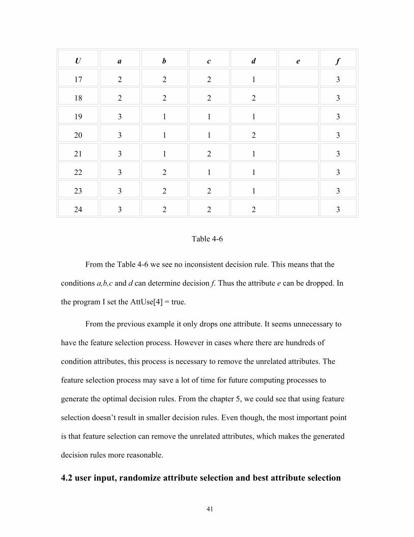
Table 4-6

From the Table 4-6 we see no inconsistent decision rule. This means that the

conditions a,b,c and d can determine decision f. Thus the attribute e can be dropped. In

the program I set the AttUse[4] = true.

From the previous example it only drops one attribute. It seems unnecessary to

have the feature selection process. However in cases where there are hundreds of

condition attributes, this process is necessary to remove the unrelated attributes. The

feature selection process may save a lot of time for future computing processes to

generate the optimal decision rules. From the chapter 5, we could see that using feature

selection doesn’t result in smaller decision rules. Even though, the most important point

is that feature selection can remove the unrelated attributes, which makes the generated

decision rules more reasonable.

4.2 user input, randomize attribute selection and best attribute selection

41

The C4.5 algorithm calculates the gain ratio for each condition attribute. It selects

the attribute whose gain ratio is the highest to divide the data set and build the decision

tree. C4.5 continues the same procedure to build the tree until all the objects in the set

belong to the same class.

If there are multiple attributes, which have the same best gain ratio, C4.5 always

selects the first attribute that appears in the table. In this case, no matter how many times

you run C4.5 using the same data it will create the same decision tree. The generated

decision tree never is the smallest possible.

For example, with data like below (Att1, Att2 and Att3):

Att1 Att2 Att3 Decision0 0 0 Y0 0 0 Y0 0 0 Y1 0 0 Y1 0 0 Y1 0 0 Y0 1 0 N0 1 0 N0 1 0 N0 1 1 Y0 1 1 Y0 1 1 Y1 0 1 N1 0 1 N1 0 1 N1 1 1 N1 1 1 N1 1 1 N1 1 1 N

42

Table 4-7

When we compute the gain ratio for these three attributes, they all have the same

gain ratio and C4.5 chooses the first attribute as the dividing point. The following image

is generated based on the original C4.5.

Figure 4-2

43

We can see that the program selects the first attribute (Att1) to start building the

tree. But it doesn't mean that the generated decision tree is the best. In the original C4.5

the position of the attribute appears in the table matters.

4.2.1 Randomize attribute selection

When using our enhanced version of C4.5 we randomly choose an attribute where

there are multiple attributes with the same best gain ratio. The program saves all the

attributes that have the same best gain ratio in an array, and randomly picks one of

attributes to divide the data set to generate the decision tree.

In this project we introduced several more attributes to the tree structure in order to

determine the best attribute. For the tree record we added the following:

1. int point (Shows how many attributes that have the same best gain ratio )

2. float *BestAttributesValue (Saves the best attribute values when there are

multiple attributes having the same gain ratio).

3. Int *BestAttributes (Saves the best attributes when there are multiple attributes

having the same gain ratio)

4. int TreeSize (Gives the size of the tree)

The way to save the attributes in the array is described here:

BestVal = -Epsilon;BestAtt = None;ForEach(Att, 0, MaxAtt) {

if ( Gain[Att] > -Epsilon ){

44

Val=Gain[Att]/Info[Att];if (Val==BestVal&&Val>-Epsilon){

Node->BestAttributesValue[Node->point]=Val; Node->BestAttributes[Node->point]=Att;Node->point++;

}

if ( Val > BestVal ) {

Node->point=0; BestAtt = Att; BestVal = Val;

Node->BestAttributesValue[Node->point]=Val; Node->BestAttributes[Node->point]=Att;Node->point++;

} }

}

In this program all the same gain ratio attributes are saved in Node ->

BestAttributes. The Node->point gives the number of the same gain ratio attributes. We

can use the following piece of code to get the random integer number from 0 to max

short get_random(int max){

int random;float x;srand((unsigned) time (NULL));random=rand();x=(float) rand()/RAND_MAX;return (int)(x*max);

}

For the above example, if we use the randomize attribute selection, we see the following output:

45

Figure 4-3

For this example, the gain ratio for every attribute is listed below.

GainRatio(Att1) = 0.099, GainRatio(Att2)=0.099 and GainRatio(Att3)=0.099.

The project uses the algorithm listed above to randomly select one attribute (Att2) as the

node to build the decision tree. The advantage of using this method is that it creates a

chance of generating a smaller tree. This randomize selection algorithm could generate

different trees each time if there are some attributes which have the same gain ratio.

4.2.2 Best Attribute selectionIn the project, I use the greedy algorithm to select the best attribute if there are

multiple attributes that have the same best gain ratio.

46

47

The algorithm goes through all the multiple attributes with the same best gain

ratio. It measures the TreeSize of the sub-trees that are built based on these multiple

attributes. The program creates a sub-tree of these candidate attributes and compares the

size of the sub-tree. It chooses the attribute with the smallest sub-tree. In this case it

generates a smaller decision tree than C4.5 alone.

The following is the code to use the greedy algorithm to find the best attribute.

BestAtt=Node -> BestAttributes [0];BestVal=Node -> BestAttributesValue[0];Node=getTree(Node, BestAtt, BestVal, Fp, Lp, Cases, NoBestClass, BestClass);TempNode = CopyTree(Node);ForEach (f,1,Node->point -1){

BestAtt=Node -> BestAttributes[f];BestVal=Node->BestAttributesValue[f];Node = getTree(Node, BestAtt, BestVal, Fp, Lp, Cases, NoBestClass, BestClass);if (Node -> TreeSize<TempNode -> TreeSize){

TempNode = CopyTree(Node);}

}Node = CopyTree(TempNode);

For the above example, if we use the greedy algorithm, we will get the following output.

48

Figure 4-4

For this example, the gain ratio for every attribute is listed below.

GainRatio(Att1) = 0.099, GainRatio(Att2)=0.099 and GainRatio(Att3)=0.099.

When using Att1 to build the sub-tree, it generates the sub-tree with size 9. If use Att2 to

build the sub-tree, it generates the sub-tree with size 9. If use Att3 to build the sub-tree, it

generates the sub-tree with size 7. The program automatically selects the best attribute

(Att3) and generates a smaller tree.

This method will not generate a better tree in all situations. It only works in cases

where there are attributes with the same gain ratio. The attributes in the data set that have

the same gain ratio normally share a similar structure. For example, it has same number

of attribute values and has same number of cases that has the same attribute values. In

this project, the program uses the decision tree generated by this method as the input to

find the Optimal Reduct. When the decision tree is smaller, the generated Optimal Reduct

will be smaller too.

49

4.2.3 User inputThe project also gives the user the control to select one of the attributes that have the

same best gain ratio.

The following is the code for user to select one attribute

printf("\n Please choose one attribute: (";ForEach(e,0,Node->point-1){

printf("%d: %s", e, AttName[Node ->BestAttributes[e]]);if(e+1==Node -> point){

printf(")\n");}

}scanf ("%d", &att);printf("\n The selected attribute is %d which is %s", att, AttName[Node->BestAttributes[att]]);BestAtt=Node -> BestAttributes[att];BestVal=Node->BestAttributesValue[att];

For the above example, if we use the user input, we will get the following output.

50

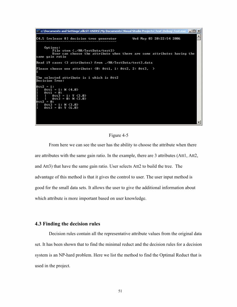
Figure 4-5

From here we can see the user has the ability to choose the attribute when there

are attributes with the same gain ratio. In the example, there are 3 attributes (Att1, Att2,

and Att3) that have the same gain ratio. User selects Att2 to build the tree. The

advantage of this method is that it gives the control to user. The user input method is

good for the small data sets. It allows the user to give the additional information about

which attribute is more important based on user knowledge.

4.3 Finding the decision rules

Decision rules contain all the representative attribute values from the original data

set. It has been shown that to find the minimal reduct and the decision rules for a decision

system is an NP-hard problem. Here we list the method to find the Optimal Reduct that is

used in the project.

51

Step 1:

Convert the decision tree generated from C4.5 to decision rules. For example, we

have a tree like below:

Att1=1: | Att3=1: N| Att3=0: YAtt1=0: | Att2=0: Y| Att2=1:| | Att3=1: Y| | Att3=0: N

After converting the tree to the rules, the rules in the table would look like the following:

Rules Att1 Att2 Att3 D

1 1 1 N

2 1 0 Y

3 0 1 1 Y

4 0 1 0 N

5 0 0 Y

Table 4-8

Step 2:

Evaluate each rule to remove the superfluous attribute-values and at the end

remove the duplicate rules from the rule set. Here is the algorithm used in this method.

ForEach object in the table //For each line in the table{

ForEach (attribute-value){drop the attribute-values in sequence; //drop one attribute at a time; check the consistency of the table;

}

52

Reduct[i]=Get the smallest attribute-value sets;EvaluateTheRule(Reduct[i]);//remove the duplicate rules

}

For example when we evaluate the rule 3 in Table 4-8, here is the steps:

1. Evaluate the rule starting from Att1 and use sequence Att1, Att2 and Att3 to

remove the superfluous attribute values. Remove Att1=0 to see if the Att2=1 and

Att3=1 could determine Decision = Y in the original decision table, Table 4-7. In

this case, it cannot determine decision. So Att1=0 cannot be removed. Remove

Att2=1, the Att1=0 and Att3=1 could determine Decision =Y in the original

decision table. So Att2=1 could be removed. Remove Att3=1 to see if Att1=0

could determine the Decision. In this case, it cannot. So Att3=1 cannot be

removed. Then the rule becomes Att1=0, Att3=1, decision is Y. The length of the

rule is 2. The final rule is Att1=0, Att3=1, decision is Y.

2. Evaluate the rule starting from Att2 and use sequence Att2, Att3 and Att1 to

remove the superfluous attribute values. Then the rule is still Att1=0, Att3=1,

decision is Y. The length of the rule is 2. It is not smaller than the rule generated

in the first step. The final rule will not be changed and it is still Att1=0, Att3=1,

decision is Y. If the length of the rule generated in this step is smaller than 2, the

final rule will be replaced with the rule generated in this step.

3. Evaluate the rule starting from Att3 and use sequence Att3, Att1, and Att2 to

remove the superfluous attribute values. The result is the same as in step 2.

4. So the final rule for rule 3 is Att1=0, Att3=1, decision is Y.

53

This method evaluates the attribute-values of conditions starting from each attribute.

For example: If one table has four attributes a,b,c,d. The program would evaluate each

rule as the following sequence: a,b,c,d and b,c,d,a and c,d,a,b and d,a,b,c. The program

removes the superfluous attribute-value for each rule and then selects the smallest as the

Rule. The following is the screen image for the generated rules.

54

Figure 4-6

From the output of the program it can be observed that it removed some

unnecessary attributes before showing the rules. For example, compare to the decision

tree, for rule 3, it removed Att2. For rule 4, it removed Att1. For rule 5, it removed Att3.

4.4 Using threshold to generate the rules

For simple decision table, the generated rules are easy to read. For above example

it has only five rules, which is very easy to understand. But for big complicated decision

table, the generated rules would be too much for user to read. For monk2 example

(monk2 has 6 attributes and 169 objects), the program will generate 81 rules, which is

very hard for user to read. So we need a rule pruning technique to filter out some rules

and make the generated rules understandable. In this project I used the threshold to filter

out the rules. Users could base on the knowledge of the data set and set the threshold

value. For example, users could ask the program to show the rules that have more than 3

instances. In the monk2 example, after set the threshold to 3, it generates 9 rules, which

cover 49 objects.

The following is the output of the program for the monk2 example.

55

56

Figure 4-7

5 Result comparison

In the project, four data sets were tested. The following list of data sets serves as

examples to illustrate how close the results compare to the minimal reduct generated by

Rough Sets. The results are also compared with the Covering Algorithm and LEM2

algorithm in Rough Sets Exploration System (Bazan et al, 2002). The first data set is

described in chapter 4.1 Table 4-1. The second data set is the monk3. The third and

fourth data sets are monk1 and monk2.

Experiment 1: The Table 4-1 is the Optician’s decisions table that is obtained from

Pawlak, Z’s book (Pawlak, 1991). It has 24 objects, 4 condition attributes and 1 decision

attribute. As explained in the book, by using the Rough Set theory, the minimal reduct of

the table has 9 rules as indicated in (Pawlak, 1991). When using the same data set as the

input of this project, it generates 9 rules too. In this case this project generates the

minimal reduct for this data set.

Experiment 2: Monk1, Monk2 and Monk3 data set (see Appendix B for the monk3 data

set)

The MONK’s problem is a collection of three binary classification problems over a six-

attribute discrete domain. This monk3 sample has 122 instances. The covering

57

algorithm in the Rough Sets Exploration System was used to generate the minimal reduct

on the Monk3 data set. It generates 18 rules. But the rules do not cover the whole data

set. It misses 28 cases in the data set. When using LEM2 algorithm in the Rough Set

Exploration System to generate the minimal reduct, it generates 41 rules that cover the

whole data set. When using the monk3 data set as the input of this project, it generates 24

rules that are better than LEM2 algorithm and can cover the whole data set.

The following are the test results from the experiments.

Data sets No.

objects

Con

atts

Covering Algorithm

No. rules Missed cases

LEM2

No. rules

This project

No. rules

Without

feature

selection

With

feature

selection

Monk1 124 6 1 95 45 28 21

Monk2 169 6 30 109 94 81 81

Monk3 122 6 18 28 41 24 27

Table 5-1

Findings: From the test we can see that using feature selection doesn’t result to a better

reduct. But the feature selection is useful to remove the unnecessary attributes to make

the generated decision rules more reasonable, because we don’t want to have the rules

with unrelated attribute values information.

Complexity comparison

58

In the Rough Sets, to find the minimal reduct or minimal decision rules is an NP-

Hard problem. Let m be the number of objects in the decision system. Let n be the

number of condition attributes in the decision system. For the first object, we need n2

steps to find the minimal attribute-values for this rule. For the second object combining

with the consideration of the first object, we need 2)2()2()2( nnn =× steps to find the

minimal attribute-values for object 1 and object2. Repeat the same calculation, we can

get that complexity for finding the minimal decision rules is O ( mn )2( )

The following is the calculation for the complexity of this project’s algorithm.

Assume the decision table has m number of objects, n number of condition attributes and

i number of maximum allowed different attribute values for each attribute.

• For feature selection, we remove the attributes in sequence to see if the rest of

table is still consistent. It has complexity O (mn).

• For generating the decision tree, maximum number of leaf can be at most m. The

maximum depth of the tree can be n. The maximum number of node in the tree

can be mn. The complexity to generate the root node is O(mni). The time to spend

on generating the root node is much longer than other node. So the worst-case

time complexity to generate the decision tree is )( 22 inmO . If we use the greedy

algorithm on generating the decision tree, the worst case is that for generating

every node, all the attributes have the same gain ratio. Because the maximum

depth of the tree is n, and it has maximum n attributes. The maximum opportunity

59

to have this situation is 2n . The complexity for generating the decision tree

becomes )( 42 inmO

• For the reduct generation, we start from every attribute and evaluate the

remaining attributes in sequence to remove the superfluous attribute values. For

example we have 3 attributes which are att1, att2 and att3. At first we evaluate the

attribute values using sequence att1, att2 and att3. The complexity to get the rules

for this case is O(mn). Next time we evaluate the attribute values using sequence

att2, att3 and att1. The third time the sequence is att3, att1 and att2. So for one

rule to remove the superfluous attribute-values, the complexity is O( 2mn ). The

maximum rules the decision table can be m. So the complexity for reduct

generation is O( 22nm )

• For removing the duplicate rules, the complexity is O( 2m ).

The total complexity for generating the Optimal Reduct is O(mn)+ )( 42 inmO + O( 22nm )

+O( 2m )= )( 42 inmO

For example one decision system has 4 attributes and 4 objects and 2 different

attribute values. When using Rough Set to get the minimal decision rules, it needs 44 )2(

= 65536 steps. When using the algorithm described here to find the Optimal Reduct, it

spends 8192244 42 =×× steps. From this example you could see that the complexity

from this algorithm is much smaller than from the Rough Sets.

60

From these experiments, we can seen that this project can quickly find the good

reduct which is very close to the minimal reduct or the same as the minimal reduct.

61

6 Conclusion

Rough Set theory is the first theory on relational database and provides many useful

concepts on data mining such as representing knowledge in a clear mathematical manner,

deriving rules only from facts present in data and reducing information systems to its

simplest form. It is very costly to get the minimal reduct from Rough Sets, which has

been shown to be an NP-hard problem.

C4.5 is a classification algorithm and it is used to generate the decision tree. The

C4.5 tree-induction algorithm provides a small decision tree and is very fast. However, it

does not always produce the smallest tree.

In this project, the C4.5 algorithm was enhanced to use the greedy algorithm to

generate the decision tree. By using this method, if the data set has multiple attributes that

have the same best gain ratio, the generated decision tree has smaller size than the result

from the original C4.5.

I use the decision tree generated by the modified version of C4.5 as input to find

an Optimal Reduct for the relational table. By testing the result on many data sets, it has

been shown that the project can quickly generate the result that is very close to or the

same as the minimal reduct, which Rough Sets generates. By comparing the result with

Rough Sets Exploration System’s covering algorithm and LEM2 algorithm, the result

from this project is better.

62

References[1] T.Y.Lin, N. Cercone. Rough Sets and data mining: analysis for imprecise data.

Boston, Mass: Kluwer Academic, c1997.

[2]Lech Polkowski, Shusaku Tsumoto, T.Y.Lin. Rough Set methods and applications:

new developments in knowledge discovery in information systems. Heidelberg; New

York: Physica-Verlag, c2000.

[3]Quinlan, J. Ross. C4.5: Programs for Machine Learning. Morgan Kaufmann, San

Mateo, CA, 1993.

[4]Zdzislaw Pawlak, Rough sets, International Journal of computer and information

science, Vol.11, No.5, 1982.

[5]W.Frawley, G. Piatetsky-Shapiro, and C. Matheus. Knowedge discovery in databases:

An overview. AI magazine, Fall issue, 1992.

[6]Margaret H. Dunham, Data Mining Introduction and Advanced Topics Prentice hall,

2003.

[7] Jiye Li and Nick Cercone, Empirical Analysis on the Geriatric Care Data Set Using

Rough Sets Theory. Technical Report, CS-2006-13, School of Comoputer Science,

University of Waterloo, April 2006.

[8] Ping Yin, Data mining on Rough Set theory using Bit Strings.Thesis, San Jose State

university, California.

[9] Jan G. Bazan, Marcin S. Szczuka, Jakub Wroblewski, A new version of rough set

exploration system. 2002.

[10] A. Skowron, C.Rauszer, The discernibility matrics and Functions in Information

System, ICS PAS Report 1/91, Technical University of Warsaw, pp. 1-44, 1991.

63

[11] T. Y. Lin, An Overview of Rough Set Theory from the Point of View of Relational

Databases, Bulletin of International Rough Set Society, Vol 1, No 1, March, 1997, 30-34.

[12] Pawlak, Z.: Rough Sets - Theoretical Aspects of Reasoning about Data. Kluwer

Academic Publishers, Dordrecht (1991).

[13] J. Komorowski, L. Polkowski, and A. Skowron. Rough Sets: A Tutorial In: Rough

Fuzzy Hybridization -- A New Trend in Decision Making, pp. 3--98, S.K. Pal, A.

Skowron, Eds, Springer.

[14] S. Krishna, Introduction to Database and Knowledge-Base Systems, World

Scientific March 1992.

[15] Kyle Loudon, Mastering Algorithms with C, August 1999.

[16] Johann Petrak, C4.5 – ofai, Internet http://www.ofai.at/~johann.petrak/c45ofai.html.

[17] Oyvind Tuseth Aasheim and Helge Grenager Solheim, Rough Sets as a Framework

for Data Mining, Knowledge Systems Group, Faculty of Computer Systems and

Telematics, The Norwegian University of Science and Technology. April 1996.

[18] Keyun Hu, Lili Diao, Yuchang Lu and Chunyi Shi, Sampling for Approximate

Reduct in very Large Datasets, Computer Science Department, Tsinghua University,

Beijing 100084, P.R.China.

[19] Subhradyuti Sarkar, How classifiers perform on the end-game chess databases,

Internet http://www.cs.ucsd.edu/~s1sarkar/Reports/CSE250B.pdf.

64

http://www.cs.ucsd.edu/~s1sarkar/Reports/CSE250B.pdf

http://www.ofai.at/~johann.petrak/c45ofai.html

Appendix A – Source code for this project Besttree.c

#include "defns.i"#include "types.i"#include "extern.i"

ItemNo *TargetClassFreq;Tree *Raw;extern Tree *Pruned;ItemNo RuleNo1;/*Number of Rules */

/**********************************************************/* *//* Grow and prune a single tree from all data*//* *//********************************************************/

OneTree()/* --------- */{ Tree FormTree(), CopyTree(); Boolean Prune();

InitialiseTreeData(); InitialiseWeights();

Raw = (Tree *) calloc(1, sizeof(Tree)); Pruned = (Tree *) calloc(1, sizeof(Tree));

AllKnown = true;

InitAttUse();if (useFeatureSelection){FeatureSelection(Item);//Write to AttUse to determine

//if the attribute will be //used in the later //calculation.

}

65

Raw[0] = FormTree(0, MaxItem); printf("\n"); PrintTree(Raw[0]);

if(generateReduct){

RuleNo1=PrintToTable3(Raw[0]);//Convert the tree to //table Reduct

GenerateOptimalRedcut(Reduct);//Through process to //delete unnecessary //attribute-value RemoveDuplicateRules(Reduct);

PrintReduct(Reduct); //Print out the reduct table}

}

/**************************************************//* *//* Remove the duplicate Rules from Reduct table *//* *//**************************************************/RemoveDuplicateRules(Reduct1)Description *Reduct1;{

int i,m,j; Boolean flag;

Description Row, Row1, Row2;ForEach(i,0,RuleNo1){

ForEach(m,i+1,RuleNo1){

flag=true;ForEach(j,0,MaxAtt){

Row1=Reduct1[i];Row2=Reduct1[m];

if(Row1[j]._discr_val!=Row2[j]._discr_val){

flag=false;break;

}}if (flag){

ForEach(j,0,MaxAtt){

Row=Reduct1[i];Row[j]._discr_val=-1;

66

}

Reduct1[m][MaxAtt+2]._cont_val+=Reduct1[i][MaxAtt+2]._cont_val;break;

}}

}}/**************************************************//* *//* Print out the reduct table *//* *//**************************************************/PrintReduct(Reduct2) Description *Reduct2;{

int i,m;short tmp=0;int rulenumber=1;

Boolean NeedtoPrint();ForEach(i,0,RuleNo1){

if(NeedtoPrint(i)==true){

printf("\nRule %d:",rulenumber);rulenumber++;ForEach(m,0,MaxAtt){

tmp=-1;tmp=DVal(Reduct2[i],m);if(tmp!=-1){

printf("\n %s = %s",AttName[m],AttValName[m][tmp]);

}}printf("\n -> class %s ( %.1f )

",ClassName[Reduct2[i][MaxAtt+1]._discr_val], CVal(Reduct2[i],MaxAtt+2));

}}

}/**************************************************//* *//* Print out all the Items /* This is used for debugging purpose *//* *//**************************************************/

67

PrintDataset(Dataset) Description *Dataset;{

int i,m;short tmp=0;int Itemnumber=1;

ForEach(i,0,MaxItem){

ForEach(m,0,MaxAtt){

tmp=DVal(Dataset[i],m);printf("\n %s =

%s",AttName[m],AttValName[m][tmp]);}

printf("\n -> class %s ( %.1f ) ",ClassName[Dataset[i][MaxAtt+1]._discr_val], CVal(Dataset[i],MaxAtt+2));

printf("Evaluation flag -> %d", DVal(Dataset[i],MaxAtt+3));}

}/**************************************************//* *//* Print out One row in the table /* This is used for debugging purpose *//* *//**************************************************/PrintOneRow(OneRow)Description OneRow;{

int m,tmp;ForEach(m,0,MaxAtt)

{tmp=DVal(OneRow,m);printf("\n %s =

%s",AttName[m],AttValName[m][tmp]);} printf("Evaluation flag from one row-> %d",

DVal(OneRow,MaxAtt+3));}

/*********************************************************//* *//* Check if we need to show the rule *//* If this row has only -1 as the data *//* this method will return false *//* *//*********************************************************/

68

Boolean NeedtoPrint(i)int i;{

int m;short tmp=0;Boolean hasdata;hasdata=false;

ForEach(m,0,MaxAtt){

tmp=DVal(Reduct[i],m);

if(tmp!=-1){hasdata=true;

}}

return hasdata;}

/*********************************************************//* *//* Init the AttUse *//* The AttUse is used to indicate if some *//* attribute is needed *//* This is for feature selection *//* *//********************************************************/InitAttUse(){

int i; AttUse=(Boolean *)malloc(MaxAtt*sizeof(Boolean));

if (AttUse == NULL){

printf("Not enough memory for AttUse memory allocation\n");exit(1);

}ForEach(i,0,MaxAtt){

AttUse[i]=false;//By default all the attributes will be necessary

}}/********************************************************//* *//* Feature selection for the Item */ /* *//*******************************************************/

69

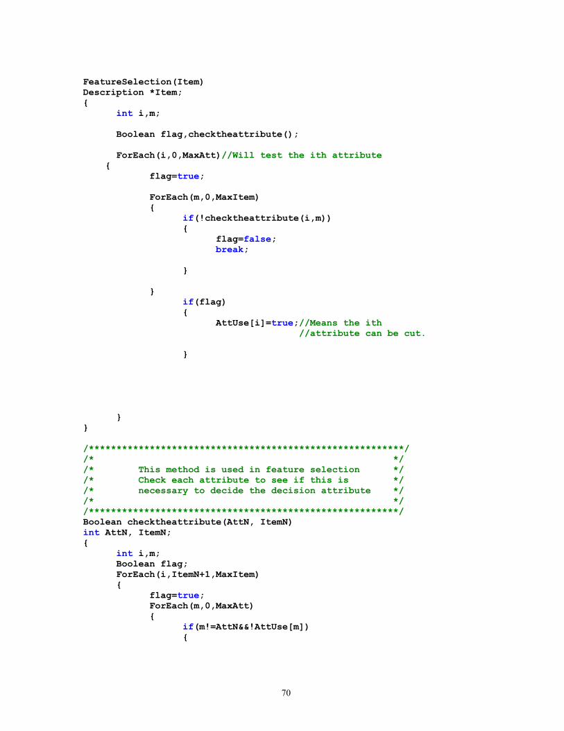
FeatureSelection(Item)Description *Item;{

int i,m;Boolean flag,checktheattribute();ForEach(i,0,MaxAtt)//Will test the ith attribute

{flag=true;ForEach(m,0,MaxItem){

if(!checktheattribute(i,m)){

flag=false;break;

}}

if(flag){

AttUse[i]=true;//Means the ith //attribute can be cut.

}

}}/*********************************************************//* *//* This method is used in feature selection */ /* Check each attribute to see if this is *//* necessary to decide the decision attribute */ /* *//********************************************************/Boolean checktheattribute(AttN, ItemN)int AttN, ItemN;{

int i,m;Boolean flag;ForEach(i,ItemN+1,MaxItem){

flag=true;ForEach(m,0,MaxAtt){

if(m!=AttN&&!AttUse[m]){

70

if(Item[i][m]._discr_val!=Item[ItemN][m]._discr_val)

{flag=false;break;

}}

}if(flag){

if(Item[i][MaxAtt+1]._discr_val!=Item[ItemN][MaxAtt+1]._discr_val)

{return false;

}}

}return true;

}

/*********************************************************//* *//* Generate the optimal reduct from the table Reduct */ /* *//********************************************************/GenerateOptimalRedcut(Reduct1)Description *Reduct1;{

Description Process();

int i,t,m,instance; CopyItem(Item); Verbosity(5){

printf("Number of Rules are %d",RuleNo1+1);}ForEach(i,0,RuleNo1){

Reduct1[i]=Process(Reduct1[i]);

if(NeedtoPrint(i)){

instance=EvaluateTheRule(Reduct1[i]);if (instance==0)//Cannot find any instance

//associate with this rule. //Needs to delete this rule.

{EmptyRule(Reduct1[i]);

71

}if (SizeOfDataSet(Dataset)==0)

//So far the rules have //covered all the cases. Need //to stop.

{ForEach(t,i+1,RuleNo1){

ForEach(m,0,MaxAtt+2){

DVal(Reduct1[t],m)=-1;}

}break;

}

}

} }/********************************************************//* *//* If the rule is a duplicate rule *//* Program need to delete the rule. *//* *//*********************************************************/EmptyRule(OneRow)Description OneRow;{

int i;ForEach(i,0,MaxAtt+2){

DVal(OneRow,i)=-1;}

}/*********************************************************//* *//* Evaluate each rule to see how many instances *//* can use this rule to get the decision and mark *//* those instances to indicate that there is some rule *//* avaiable to classify these instances. *//* *//********************************************************/ int EvaluateTheRule(Rule)Description Rule;{

int i;int t;

72

int flag;int instancecount=0;

ForEach(i,0,MaxItem) {

flag=1; if(DVal(Dataset[i],MaxAtt+3)==1) //This row hasn't

//been applied to //any rule

{ ForEach(t,0,MaxAtt) {

if(DVal(Rule,t)!=-1) {

if(DVal(Dataset[i],t)!=DVal(Rule,t))

{ flag=0;

} }

} if(flag) {

DVal(Dataset[i],MaxAtt+3)=0;//0 means that //this row has //the rule //associated.

instancecount++; }

} } CVal(Rule,MaxAtt+2)=instancecount; return instancecount; }

/***************************************************//* *//* Return the number of instances which don't have *//* the rule to classify them *//* *//*******************************************************/int SizeOfDataSet(Dataset1)Description *Dataset1;{

int i,counter=0;ForEach(i,0,MaxItem){

if(DVal(Dataset1[i],MaxAtt+3)==1){

counter++;

73

}}return counter;

}

/********************************************************//* *//* Process each row of the Reduct table to remove the *//* unnecessary attribute-value */ /* *//***************************************************/Description Process(OneRow)Description OneRow;{

Boolean checkConsistency();Description CopyRow();short oldvalue;int i;int s;int count=0;int best=0;Description WorkingRow,FinalRow;WorkingRow=CopyRow(OneRow);FinalRow=CopyRow(OneRow);ForEach(i,0,MaxAtt){ count=0;

OneRow=CopyRow(WorkingRow);ForEach(s,i,MaxAtt){

oldvalue=OneRow[s]._discr_val;if(oldvalue!=-1){

OneRow[s]._discr_val=-1;count++;if(!checkConsistency(OneRow)){

OneRow[s]._discr_val=oldvalue;count--;

}}

}ForEach(s,0,i-1){

oldvalue=OneRow[s]._discr_val;if(oldvalue!=-1){

OneRow[s]._discr_val=-1;count++;if(!checkConsistency(OneRow)){

OneRow[s]._discr_val=oldvalue;count--;

}}

}

74

if(best<count){

best=count;FinalRow=CopyRow(OneRow);

}

}OneRow=CopyRow(FinalRow);return OneRow;

} /********************************************************//* *//* Copy the Items to Dataset. And add one more flag at *//* the end of each row to indicate if row has been *//* coverd by a rule. The flag will be used in */ /* GenerateOptimalReduct method. 1 means it is not *//* coverd or not evaluated. *//* *//****************************************************/CopyItem(Item)Description *Item;{ int i;

Dataset =(Description *)calloc(MaxItem+1, sizeof(Description));ForEach(i,0,MaxItem){

Dataset[i] = (Description) calloc(MaxAtt+4, sizeof(AttValue));

Dataset[i]=CopyRow(Item[i]);DVal(Dataset[i], MaxAtt+3)=1;

}

}

/*********************************************************//* *//* Copy the Row */ /* *//******************************************************/Description CopyRow(OneRow)Description OneRow;{

int i;Description NewRow;NewRow = (Description)

calloc(MaxAtt+3, sizeof(AttValue));ForEach (i,0,MaxAtt+1)

75

{DVal(NewRow, i) = OneRow[i]._discr_val;

}CVal(NewRow,MaxAtt+2)=CVal(OneRow,MaxAtt+2);return NewRow;

}/******************************************************//* *//* Test each attribute-value to see if *//* it would affect the consistency of the *//* whole table *//* *//*****************************************************/Boolean checkConsistency(OneRow)Description OneRow;{

int i,m;Boolean flag;ForEach(i,0,MaxItem)//For Item{

flag=true;ForEach(m,0,MaxAtt){

if(OneRow[m]._discr_val!=-1){

if(OneRow[m]._discr_val!=Item[i][m]._discr_val){

flag=false;}

}}if(flag)

{

if(OneRow[MaxAtt+1]._discr_val!=Item[i][MaxAtt+1]._discr_val&&flag)

{return false;

}}

}

return true;}

76

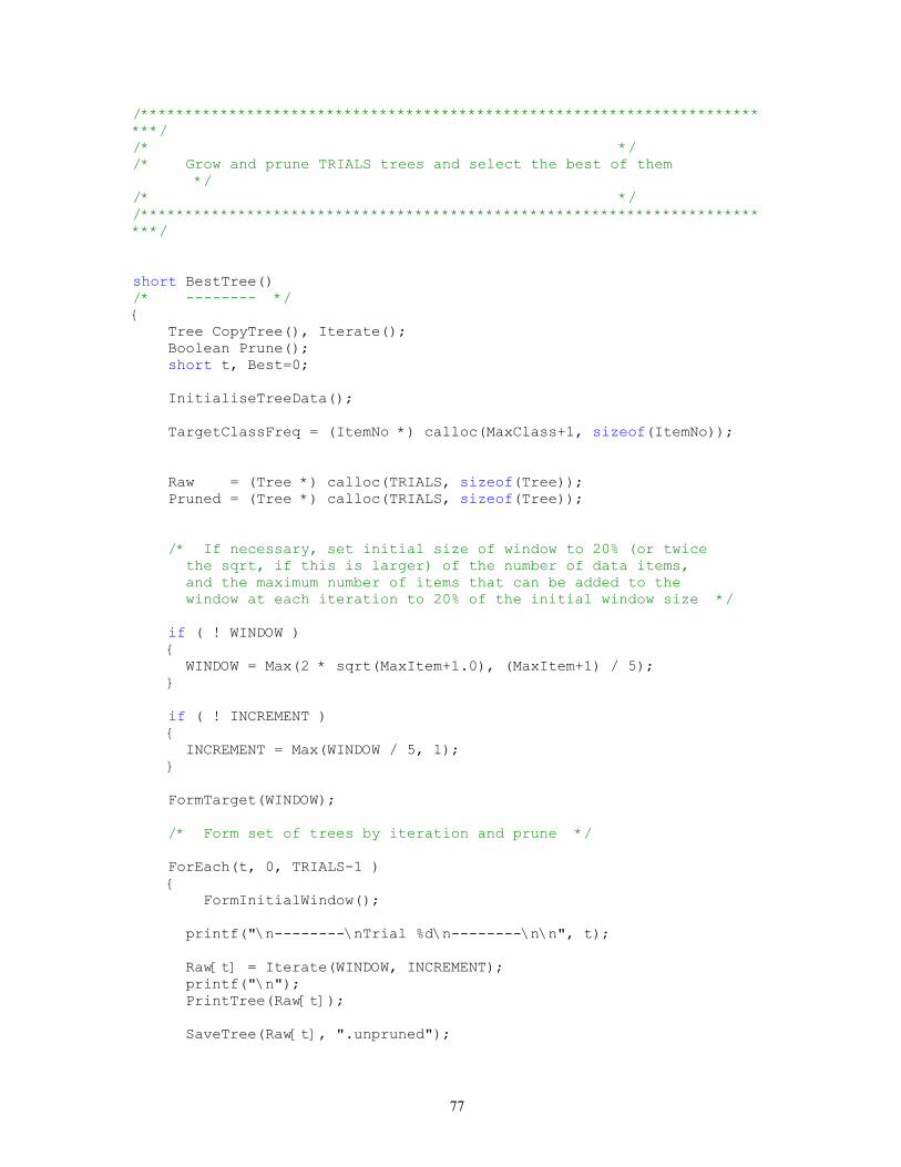
/*************************************************************************//* *//* Grow and prune TRIALS trees and select the best of them

*//* *//*************************************************************************/

short BestTree()/* -------- */{ Tree CopyTree(), Iterate(); Boolean Prune(); short t, Best=0;

InitialiseTreeData();

TargetClassFreq = (ItemNo *) calloc(MaxClass+1, sizeof(ItemNo));

Raw = (Tree *) calloc(TRIALS, sizeof(Tree)); Pruned = (Tree *) calloc(TRIALS, sizeof(Tree));

/* If necessary, set initial size of window to 20% (or twicethe sqrt, if this is larger) of the number of data items,and the maximum number of items that can be added to thewindow at each iteration to 20% of the initial window size */

if ( ! WINDOW ) {

WINDOW = Max(2 * sqrt(MaxItem+1.0), (MaxItem+1) / 5); }

if ( ! INCREMENT ) {

INCREMENT = Max(WINDOW / 5, 1); }

FormTarget(WINDOW);

/* Form set of trees by iteration and prune */

ForEach(t, 0, TRIALS-1 ) { FormInitialWindow();

printf("\n--------\nTrial %d\n--------\n\n", t);

Raw[t] = Iterate(WINDOW, INCREMENT);printf("\n");PrintTree(Raw[t]);

SaveTree(Raw[t], ".unpruned");

77

Pruned[t] = CopyTree(Raw[t]);if ( Prune(Pruned[t]) ){ printf("\nSimplified "); PrintTree(Pruned[t]);}

if ( Pruned[t]->Errors < Pruned[Best]->Errors ){ Best = t;}

} printf("\n--------\n");

return Best;}

/*************************************************************************//* *//* The windowing approach seems to work best when the class

*//* distribution of the initial window is as close to uniform as *//* possible. FormTarget generates this initial target distribution,

*//* setting up a TargetClassFreq value for each class.

*//* *//*************************************************************************/

FormTarget(Size)/* ----------- */ ItemNo Size;{ ItemNo i, *ClassFreq; ClassNo c, Smallest, ClassesLeft=0;

ClassFreq = (ItemNo *) calloc(MaxClass+1, sizeof(ItemNo));

/* Generate the class frequency distribution */

ForEach(i, 0, MaxItem) {

ClassFreq[ Class(Item[i]) ]++; }

/* Calculate the no. of classes of which there are items */

ForEach(c, 0, MaxClass) {

if ( ClassFreq[c] ){

78

ClassesLeft++;}else{ TargetClassFreq[c] = 0;}

}

while ( ClassesLeft ) {

/* Find least common class of which there are some items */

Smallest = -1;ForEach(c, 0, MaxClass){ if ( ClassFreq[c] &&

( Smallest < 0 || ClassFreq[c] < ClassFreq[Smallest] ) ) {

Smallest = c; }}

/* Allocate the no. of items of this class to use in the window */

TargetClassFreq[Smallest] = Min(ClassFreq[Smallest], Round(Size/ClassesLeft));

ClassFreq[Smallest] = 0;

Size -= TargetClassFreq[Smallest];ClassesLeft--;

}

free(ClassFreq);}

/*************************************************************************//* *//* Form initial window, attempting to obtain the target class profile

*//* in TargetClassFreq. This is done by placing the targeted number *//* of items of each class at the beginning of the set of data items.

*//* *//*************************************************************************/

FormInitialWindow()/* ------------------- */{ ItemNo i, Start=0, More;

79

ClassNo c; void Swap();

Shuffle();


More = TargetClassFreq[c];

for ( i = Start ; More ; i++ ){ if ( Class(Item[i]) == c ) {

Swap(Start, i);Start++;More--;

}}

}}

/*************************************************************************//* *//* Shuffle the data items randomly *//* *//*************************************************************************/

Shuffle()/* ------- */{ ItemNo This, Alt, Left; Description Hold;

This = 0; for( Left = MaxItem+1 ; Left ; ) { Alt = This + (Left--) * ((rand()&32767) / 32768.0); Hold = Item[This]; Item[This++] = Item[Alt]; Item[Alt] = Hold; }}

/*************************************************************************//* *//* Grow a tree iteratively with initial window size Window and

*//* initial window increment IncExceptions. *//* */

80

/* Construct a classifier tree using the data items in the *//* window, then test for the successful classification of other *//* data items by this tree. If there are misclassified items,

*//* put them immediately after the items in the window, increase *//* the size of the window and build another classifier tree, and *//* so on until we have a tree which successfully classifies all *//* of the test items or no improvement is apparent. *//* *//* On completion, return the tree which produced the least errors.

*//* *//*************************************************************************/

Tree Iterate(Window, IncExceptions)/* ------- */ ItemNo Window, IncExceptions;{ Tree Classifier, BestClassifier=Nil, FormTree(); ItemNo i, Errors, TotalErrors, BestTotalErrors=MaxItem+1,

Exceptions, Additions; ClassNo Assigned, Category(); short Cycle=0; void Swap();

printf("Cycle Tree -----Cases----"); printf(" -----------------Errors-----------------\n"); printf(" size window other"); printf(" window rate other rate total rate\n"); printf("----- ---- ------ ------"); printf(" ------ ---- ------ ---- ------ ----\n");

do {

/* Build a classifier tree with the first Window items */

InitialiseWeights();AllKnown = true;Classifier = FormTree(0, Window-1);

/* Error analysis */

Errors = Round(Classifier->Errors);

/* Move all items that are incorrectly classified by the classifier tree to immediately after the items in the current window. */

Exceptions = Window;ForEach(i, Window, MaxItem){ Assigned = Category(Item[i], Classifier); if ( Assigned != Class(Item[i]) ) {

Swap(Exceptions, i);

81

Exceptions++; }}

Exceptions -= Window;TotalErrors = Errors + Exceptions;

/* Print error analysis */

printf("%3d %7d %8d %6d %8d%5.1f%% %6d%5.1f%% %6d%5.1f%%\n", ++Cycle, TreeSize(Classifier), Window, MaxItem-Window+1, Errors, 100*(float)Errors/Window, Exceptions, 100*Exceptions/(MaxItem-Window+1.001), TotalErrors, 100*TotalErrors/(MaxItem+1.0));

/* Keep track of the most successful classifier tree so far */

if ( ! BestClassifier || TotalErrors < BestTotalErrors ){ if ( BestClassifier ) ReleaseTree(BestClassifier); BestClassifier = Classifier; BestTotalErrors = TotalErrors;

}else{ ReleaseTree(Classifier);}

/* Increment window size */

Additions = Min(Exceptions, IncExceptions);Window = Min(Window + Max(Additions, Exceptions / 2), MaxItem +

1); } while ( Exceptions );

return BestClassifier;}

/*************************************************************************//* *//* Print report of errors for each of the trials *//* *//*************************************************************************/

Evaluate(CMInfo, Saved)/* -------- */ Boolean CMInfo; short Saved;{ ClassNo RealClass, PrunedClass, Category(); short t; ItemNo *ConfusionMat, i, RawErrors, PrunedErrors;

82

if ( CMInfo ) {

ConfusionMat = (ItemNo *) calloc((MaxClass+1)*(MaxClass+1), sizeof(ItemNo));

}

printf("\n");

if ( TRIALS > 1 ) {

printf("Trial\t Before Pruning After Pruning\n");printf("-----\t---------------- ---------------------------\n");

} else {

printf("\t Before Pruning After Pruning\n");printf("\t---------------- ---------------------------\n");

} printf("\tSize Errors Size Errors Estimate\n\n");

ForEach(t, 0, TRIALS-1) {

RawErrors = PrunedErrors = 0;

ForEach(i, 0, MaxItem){ RealClass = Class(Item[i]);

//PrintTree(Raw[t]);

if ( Category(Item[i], Raw[t]) != RealClass ) RawErrors++;

PrunedClass = Category(Item[i], Pruned[t]);

if ( PrunedClass != RealClass ) PrunedErrors++;

if ( CMInfo && t == Saved ) {

ConfusionMat[RealClass*(MaxClass+1)+PrunedClass]++; }}

if ( TRIALS > 1 ){ printf("%4d", t);}

printf("\t%4d %3d(%4.1f%%) %4d %3d(%4.1f%%) (%4.1f%%)%s\n", TreeSize(Raw[t]), RawErrors, 100.0*RawErrors /

(MaxItem+1.0), TreeSize(Pruned[t]), PrunedErrors, 100.0*PrunedErrors /

(MaxItem+1.0), 100 * Pruned[t]->Errors / Pruned[t]->Items, ( t == Saved ? " <<" : "" ));

}

83

if ( CMInfo ) {

PrintConfusionMatrix(ConfusionMat);free(ConfusionMat);

}}

build.c

/*************************************************************************//* *//* Central tree-forming algorithm incorporating all criteria *//* ---------------------------------------------------------

*//* *//*************************************************************************/

#include "defns.i"#include "types.i"#include "extern.i"

ItemCount*Weight, /* Weight[i] = current fraction of item i */**Freq, /* Freq[x][c] = no. items of class c with

outcome x */*ValFreq, /* ValFreq[x] = no. items with outcome x */*ClassFreq; /* ClassFreq[c] = no. items of class c */

float*Gain, /* Gain[a] = info gain by split on att a */*Info, /* Info[a] = potential info of split on att a */*Bar, /* Bar[a] = best threshold for contin att a */*UnknownRate; /* UnknownRate[a] = current unknown rate for

att a */

Boolean*Tested, /* Tested[a] set if att a has already been tested */MultiVal; /* true when all atts have many values */

/* External variables initialised here */

extern float*SplitGain, /* SplitGain[i] = gain with att value of item i as

threshold */*SplitInfo; /* SplitInfo[i] = potential info ditto */

extern ItemCount*Slice1, /* Slice1[c] = saved values of Freq[x][c] in

subset.c */

84

*Slice2; /* Slice2[c] = saved values of Freq[y][c] */

extern Set**Subset; /* Subset[a][s] = subset s for att a */

extern short*Subsets; /* Subsets[a] = no. subsets for att a */

int level;int att;

/*************************************************************************//* *//* Allocate space for tree tables *//* *//*************************************************************************/

InitialiseTreeData()/* ------------------ */{ DiscrValue v; Attribute a;

Tested = (char *) calloc(MaxAtt+1, sizeof(char));

Gain = (float *) calloc(MaxAtt+1, sizeof(float)); Info = (float *) calloc(MaxAtt+1, sizeof(float)); Bar = (float *) calloc(MaxAtt+1, sizeof(float));

Subset = (Set **) calloc(MaxAtt+1, sizeof(Set *));

ForEach(a, 0, MaxAtt) {

if ( MaxAttVal[a] ){ Subset[a] = (Set *) calloc(MaxDiscrVal+1, sizeof(Set));

ForEach(v, 0, MaxAttVal[a]) {

Subset[a][v] = (Set) malloc((MaxAttVal[a]>>3) + 1);

}}

} Subsets = (short *) calloc(MaxAtt+1, sizeof(short));

SplitGain = (float *) calloc(MaxItem+1, sizeof(float)); SplitInfo = (float *) calloc(MaxItem+1, sizeof(float));

Weight = (ItemCount *) calloc(MaxItem+1, sizeof(ItemCount));

85

Freq = (ItemCount **) calloc(MaxDiscrVal+1, sizeof(ItemCount *)); ForEach(v, 0, MaxDiscrVal) {

Freq[v] = (ItemCount *) calloc(MaxClass+1, sizeof(ItemCount));

}

ValFreq = (ItemCount *) calloc(MaxDiscrVal+1, sizeof(ItemCount)); ClassFreq = (ItemCount *) calloc(MaxClass+1, sizeof(ItemCount));

Slice1 = (ItemCount *) calloc(MaxClass+2, sizeof(ItemCount)); Slice2 = (ItemCount *) calloc(MaxClass+2, sizeof(ItemCount));

UnknownRate = (float *) calloc(MaxAtt+1, sizeof(float));

/* Check whether all attributes have many discrete values */

MultiVal = true; if ( ! SUBSET ) {

for ( a = 0 ; MultiVal && a <= MaxAtt ; a++ ){ if ( SpecialStatus[a] != IGNORE ) {

MultiVal = MaxAttVal[a] >= 0.3 * (MaxItem + 1); }}

}}

/*************************************************************************//* *//* Initialise the weight of each item *//* *//*************************************************************************/

InitialiseWeights()/* ----------------- */{ ItemNo i;

ForEach(i, 0, MaxItem) { Weight[i] = 1.0; }}

/*************************************************************************/

86

/* *//* Build a decision tree for the cases Fp through Lp:

*//* *//* - It only evaluates the attributes which have been /* marked necessary after feature selection. *//* If user didn't use the feature selection, *//* all the attributes will be evaluated. */

/* - Depend on users options, it builds the decision *//* tree based on the randomly choose the attribute, *//* user input or best attribute when there are some *//* attributes having the same gain ratio *//* *//*******************************************************/

Tree FormTree(Fp, Lp)/* --------- */ ItemNo Fp, Lp; { ItemNo i, Kp, Ep, Group(); ItemCount Cases, NoBestClass, KnownCases, CountItems(); float Factor, BestVal, Val, AvGain=0, Worth(); Attribute Att, BestAtt, Possible=0; ClassNo c, BestClass; Tree Node,Leaf(),SubTree(),TempNode,CopyNode(); DiscrValue v; Boolean PrevAllKnown;

short a=0, b=0, get_random();int atest=0, f, d=10;ItemNo e;Tree ChildNode;

Cases = CountItems(Fp, Lp);

/* Generate the class frequency distribution */


ClassFreq[c] = 0; } ForEach(i, Fp, Lp) {

ClassFreq[ Class(Item[i]) ] += Weight[i]; }

/* Find the most frequent class */

BestClass = 0; ForEach(c, 0, MaxClass) {

if ( ClassFreq[c] > ClassFreq[BestClass] )

87

{ BestClass = c;}

} NoBestClass = ClassFreq[BestClass];

Node = Leaf(ClassFreq, BestClass, Cases, Cases - NoBestClass);

/* If all cases are of the same class or there are not enoughcases to divide, the tree is a leaf */

if ( NoBestClass == Cases || Cases < 2 * MINOBJS ) {

return Node; }

Verbosity(1) printf("\n%d items, total weight %.1f\n", Lp - Fp + 1, Cases);

/* For each available attribute, find the information and gain */

ForEach(Att, 0, MaxAtt) {

Gain[Att] = -Epsilon;

if(!AttUse[Att])// Check if the attribute has be marked as unnecessary during the feature selection

{if ( SpecialStatus[Att] == IGNORE ) continue;

if ( MaxAttVal[Att] ){

/* discrete valued attribute */

if ( SUBSET && MaxAttVal[Att] > 2 ){EvalSubset(Att, Fp, Lp, Cases);}elseif ( ! Tested[Att] ){

EvalDiscreteAtt(Att, Fp, Lp, Cases);}

}else{

/* continuous attribute */

EvalContinuousAtt(Att, Fp, Lp);}

}

/* Update average gain, excluding attributes with very many values */

/* So if one attribute has differnt values more than 30% of the all the items, ignore it*/

88

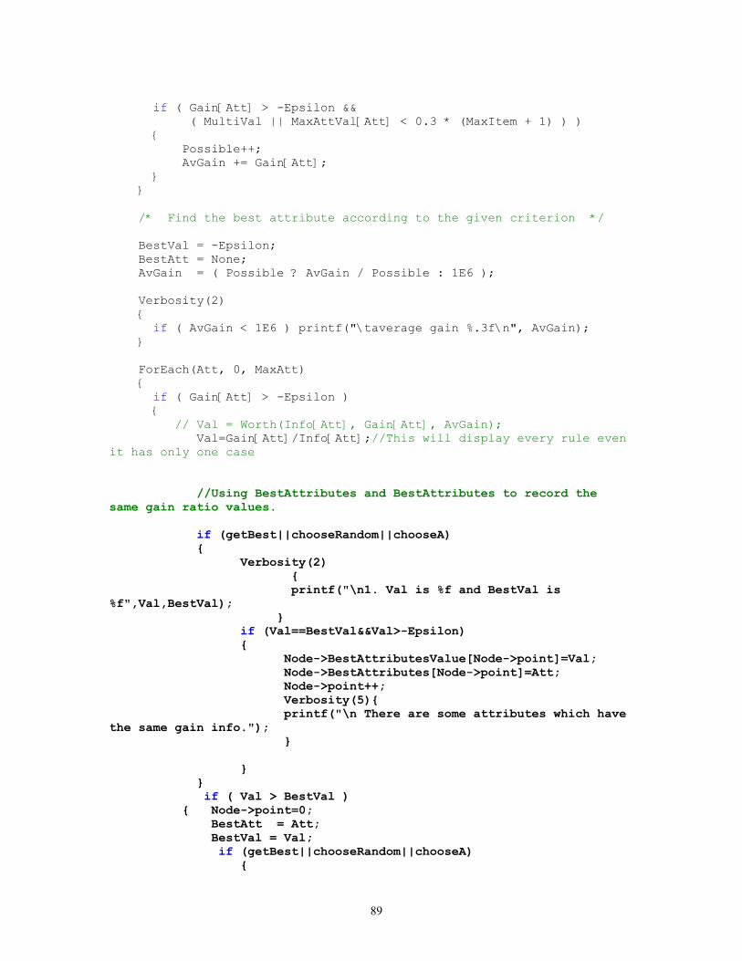
if ( Gain[Att] > -Epsilon && ( MultiVal || MaxAttVal[Att] < 0.3 * (MaxItem + 1) ) ){ Possible++; AvGain += Gain[Att];}

}

/* Find the best attribute according to the given criterion */

BestVal = -Epsilon; BestAtt = None; AvGain = ( Possible ? AvGain / Possible : 1E6 );

Verbosity(2) {

if ( AvGain < 1E6 ) printf("\taverage gain %.3f\n", AvGain); }


if ( Gain[Att] > -Epsilon ){ // Val = Worth(Info[Att], Gain[Att], AvGain);

Val=Gain[Att]/Info[Att];//This will display every rule even it has only one case

//Using BestAttributes and BestAttributes to record the

same gain ratio values.if (getBest||chooseRandom||chooseA){

Verbosity(2) { printf("\n1. Val is %f and BestVal is

%f",Val,BestVal); }if (Val==BestVal&&Val>-Epsilon){

Node->BestAttributesValue[Node->point]=Val; Node->BestAttributes[Node->point]=Att;Node->point++;Verbosity(5){printf("\n There are some attributes which have

the same gain info.");}

}} if ( Val > BestVal )

{ Node->point=0; BestAtt = Att; BestVal = Val;

if (getBest||chooseRandom||chooseA){

89

Node->BestAttributesValue[Node->point]=Val; Node->BestAttributes[Node->point]=Att;Node->point++;}

}

}

}

Verbosity(5){ printf("\nThere are %d best attributes ",Node->point);}//Randomly get the attribute when there are some//attributes having the same gain ratio.if (Node->point>1&&chooseRandom){b=get_random(Node->point);Verbosity(5) { printf("\n The random is %d",b); }

BestAtt=Node->BestAttributes[b];BestVal=Node->BestAttributesValue[b];}//User input to choose the attribute when there are some //attributes having the same gain ratioif (Node->point>1&&chooseA){ printf("\nPlease choose one attribute: (");

ForEach(e,0,Node->point-1){

printf("%d: %s, ",e,AttName[Node->BestAttributes[e]]);if (e+1==Node->point){

printf(" )\n");}

}scanf("%d", &att);printf("\nThe selected attribute is %d which is %s",att,

AttName[Node->BestAttributes[att]]); BestAtt=Node->BestAttributes[att];

BestVal=Node->BestAttributesValue[att];}

/* Decide whether to branch or not */

// Get the best attribute when there are some

90

// attributes having the same gain ratio.if(Node->point>1&&getBest){ if(BestAtt!=None)

{BestAtt=Node->BestAttributes[0];BestVal=Node->BestAttributesValue[0];}ChildNode=CopyTree(SubTree(Node,BestAtt, BestVal, Fp, Lp, Cases,

NoBestClass, BestClass));TempNode=CopyTree(ChildNode);

ReleaseTree(ChildNode); Verbosity(5){

PrintTree(TempNode);} ForEach(f, 1, Node->point-1){

Verbosity(5){printf("\nSelect the %d attribute as the best Attribute,

which is %s", f, AttName[Node->BestAttributes[f]]);//The BestAttribute cannot be reacess, because it's reallocated before and reassign the data.

}BestAtt=Node->BestAttributes[f];BestVal=Node->BestAttributesValue[f];

ChildNode=CopyTree(SubTree(Node,BestAtt, BestVal, Fp, Lp, Cases,

NoBestClass, BestClass));

Verbosity(5){PrintTree(ChildNode);

}//compare the treesize for the subtree.if(ChildNode->TreeSize<TempNode->TreeSize){

//pick the smallest subtree based on the selected attribute. TempNode=CopyTree(ChildNode);

}ReleaseTree(ChildNode);

}

//Found the smallest subtree based on all the attributes which having the same gain ratio. Node=CopyTree(TempNode); ReleaseTree(TempNode);

91

}else //didn't use getBest option.{Node=SubTree(Node,BestAtt, BestVal, Fp, Lp, Cases, NoBestClass, BestClass);Verbosity(5){

PrintTree(Node);}

}

return Node;}

/*****************************************************************************//* *//* Build a subtree for the Node: *//* *//* - if all cases are of the same class, the subtree is a leaf and so

*//* the leaf is returned labelled with this class *//* *//* - for each attribute, calculate the potential information provided

*//* by a test on the attribute (based on the probabilities of each

*//* case having a particular value for the attribute), and the gain

*//* in information that would result from a test on the attribute

*//* (based on the probabilities of each case with a particular *//* value for the attribute being of a particular class) *//* *//* - on the basis of these figures, and depending on the current *//* selection criterion, find the best attribute to branch on. *//* Note: this version will not allow a split on an attribute *//* unless two or more subsets have at least MINOBJS items. *//* *//* - try branching and test whether better than forming a leaf

*//* *//*****************************************************************************/

Tree SubTree(Node,BestAtt, BestVal, Fp, Lp, Cases, NoBestClass, BestClass)

Attribute BestAtt; float BestVal;

92

ItemNo Fp,Lp; Tree Node; ItemCount Cases, NoBestClass; ClassNo BestClass;

{

ItemCount KnownCases;ItemNo Ep,i,Kp;float Factor;Boolean PrevAllKnown;DiscrValue v;

if ( BestAtt != None ) {

Verbosity(1){ printf("\n\tbest attribute %s", AttName[BestAtt]); if ( ! MaxAttVal[BestAtt] ) {

printf(" cut %.3f", Bar[BestAtt]); } printf(" inf %.3f gain %.3f val %.3f\n",

Info[BestAtt], Gain[BestAtt], BestVal);}

/* Build a node of the selected test */

if ( MaxAttVal[BestAtt] ){ /* Discrete valued attribute */

if ( SUBSET && MaxAttVal[BestAtt] > 2 ) { SubsetTest(Node, BestAtt); } else { DiscreteTest(Node, BestAtt); }}else{ /* Continuous attribute */

ContinTest(Node, BestAtt);}

/* Remove unknown attribute values */

PrevAllKnown = AllKnown;

Kp = Group(0, Fp, Lp, Node) + 1;if ( Kp != Fp ) AllKnown = false;KnownCases = Cases - CountItems(Fp, Kp-1);UnknownRate[BestAtt] = (Cases - KnownCases) / (Cases + 0.001);

93

Verbosity(1){ if ( UnknownRate[BestAtt] > 0 ) {

printf("\tunknown rate for %s = %.3f\n", AttName[BestAtt], UnknownRate[BestAtt]);

}}

/* Recursive divide and conquer */

++Tested[BestAtt];

Ep = Kp - 1;Node->Errors = 0;

ForEach(v, 1, Node->Forks){ Ep = Group(v, Kp, Lp, Node);

if ( Kp <= Ep ) {

Factor = CountItems(Kp, Ep) / KnownCases;

ForEach(i, Fp, Kp-1){ Weight[i] *= Factor;}

Node->Branch[v] = FormTree(Fp, Ep);

Node->Errors += Node->Branch[v]->Errors;

Group(0, Fp, Ep, Node);ForEach(i, Fp, Kp-1){ Weight[i] /= Factor;}

} else {

Node->Branch[v] = Leaf(Node->ClassDist, BestClass, 0.0, 0.0);

}}

--Tested[BestAtt];AllKnown = PrevAllKnown;

/* See whether we would have been no worse off with a leaf */

if ( Node->Errors >= Cases - NoBestClass - Epsilon ){ Verbosity(1)

printf("Collapse tree for %d items to leaf %s\n", Lp - Fp + 1, ClassName[BestClass]);

94

Node->NodeType = 0;}

} else {

Verbosity(1) printf("\tno sensible splits %.1f/%.1f\n",

Cases, Cases - NoBestClass); }

Verbosity(5){printf("The Node's Size is %d. And the tested attribute is:

%d",Node->TreeSize, Node->Tested);}Node->TreeSize=TreeSize(Node);

return Node;}

/********************************************************///* *//* Get the random number for the array *//* *//***************************************************/short get_random(int max){short tt=1;int random;float x;

srand((unsigned)time(NULL));random=rand();x=(float)rand()/RAND_MAX;

tt=(int)(x*max); return tt;}/*************************************************************************//* *//* Group together the items corresponding to branch V of a test *//* and return the index of the last such *//* *//* Note: if V equals zero, group the unknown values *//* *//*************************************************************************/

ItemNo Group(V, Fp, Lp, TestNode)/* ----- */ DiscrValue V; ItemNo Fp, Lp; Tree TestNode;{ ItemNo i;

95

Attribute Att; float Thresh; Set SS; void Swap();

Att = TestNode->Tested;

if ( V ) {

/* Group items on the value of attribute Att, and depending on the type of branch */

switch ( TestNode->NodeType ){ case BrDiscr:

ForEach(i, Fp, Lp){ if ( DVal(Item[i], Att) == V ) Swap(Fp++, i);}break;

case ThreshContin:

Thresh = TestNode->Cut;ForEach(i, Fp, Lp){ if ( (CVal(Item[i], Att) <= Thresh) == (V == 1) )

Swap(Fp++, i);}break;

case BrSubset:

SS = TestNode->Subset[V];ForEach(i, Fp, Lp){ if ( In(DVal(Item[i], Att), SS) ) Swap(Fp++, i);}break;

} } else {

/* Group together unknown values */

switch ( TestNode->NodeType ){ case BrDiscr: case BrSubset:

ForEach(i, Fp, Lp){ if ( ! DVal(Item[i], Att) ) Swap(Fp++, i);}break;

96

case ThreshContin:

ForEach(i, Fp, Lp){ if ( CVal(Item[i], Att) == Unknown ) Swap(Fp++, i);}break;

} }

return Fp - 1;}

/*************************************************************************//* *//* Return the total weight of items from Fp to Lp *//* *//*************************************************************************/

ItemCount CountItems(Fp, Lp)/* ---------- */ ItemNo Fp, Lp;{ register ItemCount Sum=0.0, *Wt, *LWt;

if ( AllKnown ) return Lp - Fp + 1;

for ( Wt = Weight + Fp, LWt = Weight + Lp ; Wt <= LWt ; ) {

Sum += *Wt++; }

return Sum;}

/*************************************************************************//* *//* Exchange items at a and b *//* *//*************************************************************************/

void Swap(a,b)/* ---- */ ItemNo a, b;{ register Description Hold; register ItemCount HoldW;

97

Hold = Item[a]; Item[a] = Item[b]; Item[b] = Hold;

HoldW = Weight[a]; Weight[a] = Weight[b]; Weight[b] = HoldW;}

trees.c

/*************************************************************************//* *//* Routines for displaying, building, saving and restoring trees

*//* -------------------------------------------------------------

*//* *//*************************************************************************/

#include "defns.i"#include "types.i"#include "extern.i"#include <stdlib.h>

#define Tab "| "#define TabSize 4

#define Width 80 /* approx max width of printed trees */

/* If lines look like getting too long while a tree is being printed, subtrees are broken off and printed separately after the main tree is finished */

short Subtree; /* highest subtree to be printed */Tree Subdef[100]; /* pointers to subtrees */

FILE *TRf = 0, *fopen(); /* file pointer for tree i/o */char Fn[500]; /* file name */

extern Boolean PRINTTREE;

extern String ModelSuffix;

char suffixbuf[256];

#define Inc1 2048Description TempRule;

98

ItemNo RuleNumber=0;

/*************************************************//* *//* Save the Tree as table format *//* For one path from the tree root to leaf, *//* if it didn't mention a node, the node *//* in the table would have value of -1 *//* *//***************************************************/ItemNo PrintToTable3(T)

Tree T; {

Boolean isWrited(); DiscrValue v,MaxV; ItemNo i=0, ItemSpace1=0; T->Writed=isWrited(T); MaxV=T->Forks;

//Assign the space for Reduct. if ( i >= ItemSpace1 )

{if ( ItemSpace1 ){ItemSpace1 += Inc1;Reduct = (Description *)

realloc(Reduct, ItemSpace1*sizeof(Description));

}else{Reduct = (Description *)

malloc((ItemSpace1=Inc1)*sizeof(Description));}

} while(!T->Writed) {

TempRule = (Description) calloc(MaxAtt+2, sizeof(AttValue));initRule(TempRule);

ShowBranch3(T);//printf("\n");RuleNumber++;

} return RuleNumber-1;

}/**************************************************//* *//* Initial the TempRule and give the */

99

/* -1 as default value *//* *//**************************************************/ initRule(TempRule)

Description TempRule; {

int i; ForEach(i,0,MaxAtt+1) {

DVal(TempRule,i)=-1; }

}/***********************************************//* *//* Recursively assign the data for Reduct /* table based on the tree data */ /* *//********************************************/ ShowBranch3(T)

Tree T; {

Attribute Att; DiscrValue i,v,MaxV; int getNotWritedBranch(),BranchNo, Which(),temp;

MaxV=T->Forks; ForEach(v,1,MaxV) { Att=T->Tested;

if (T->Forks){

BranchNo=getNotWritedBranch(T);if (BranchNo!=0){

printf("%s = %s:", AttName[Att],

AttValName[Att][BranchNo]);

if (AttValName[Att][BranchNo]!=NULL){

temp=Which(AttValName[Att][BranchNo],AttValName[Att],1,MaxAttVal[Att]);DVal(TempRule,Att)=temp;}

100

ShowBranch3(T->Branch[BranchNo]);}T->Writed=isWrited(T);

}else {

printf("( %s )", ClassName[T->Leaf]);}break;

} if (!T->Forks){

DVal(TempRule,MaxAtt+1)=T->Leaf;CVal(TempRule,MaxAtt+2)=T->Items;

if (T->Items <=THRESHOLD) //The threshold{ initRule(TempRule);}Reduct[RuleNumber]=TempRule;T->Writed=true;

} }/**************************************************//* *//* Check if the branch is writed *//* *//**************************************************/ int getNotWritedBranch(T)

Tree T; {

DiscrValue v; ForEach(v,1,T->Forks) {

if (!T->Branch[v]->Writed) {

return v; }

} return 0;

}/***********************************************//* *//* Check if the tree is writed *//* *//*****************************************************/ Boolean isWrited(T)

Tree T; {

DiscrValue v,MaxV; Boolean flag=true; if(!T->Forks){

return false;

101

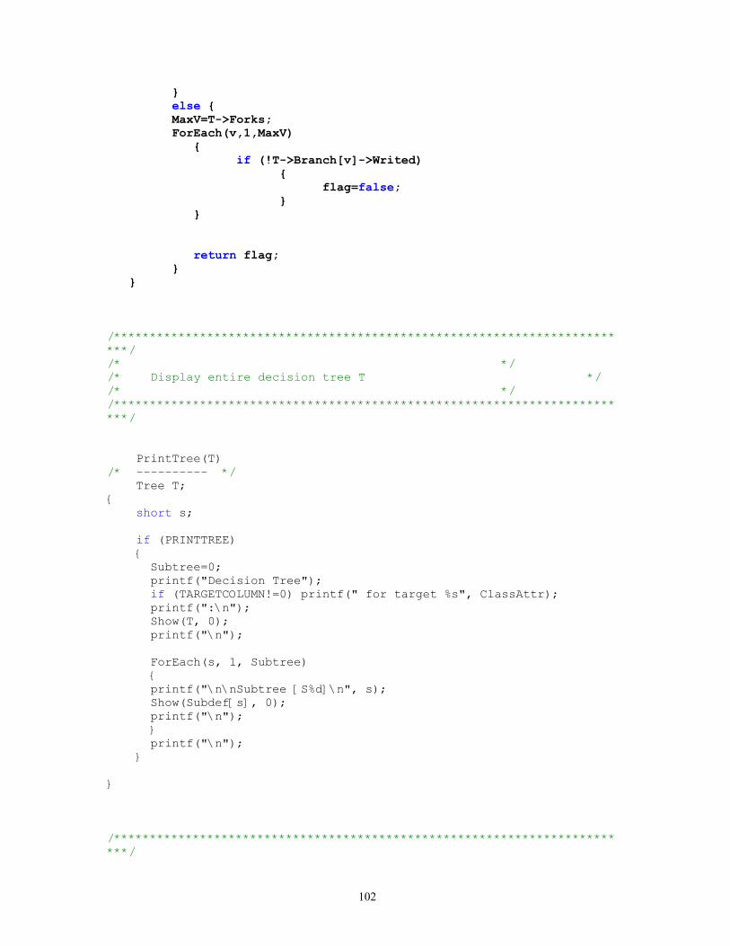
} else { MaxV=T->Forks; ForEach(v,1,MaxV)

{if (!T->Branch[v]->Writed)

{flag=false;

}}

return flag;

} }

/*************************************************************************//* *//* Display entire decision tree T *//* *//*************************************************************************/

PrintTree(T)/* ---------- */ Tree T;{ short s;

if (PRINTTREE) { Subtree=0; printf("Decision Tree"); if (TARGETCOLUMN!=0) printf(" for target %s", ClassAttr); printf(":\n"); Show(T, 0); printf("\n");

ForEach(s, 1, Subtree) { printf("\n\nSubtree [S%d]\n", s);

Show(Subdef[s], 0);printf("\n");

} printf("\n"); }

}

/*************************************************************************/

102

/* *//* Display the tree T with offset Sh *//* *//*************************************************************************/

Show(T, Sh)/* ---- */ Tree T; short Sh;{ DiscrValue v, MaxV; short MaxLine();

if ( T->NodeType ) {

/* See whether separate subtree needed */

if ( T != Nil && Sh && Sh * TabSize + MaxLine(T) > Width ){ if ( Subtree < 99 ) {

Subdef[++Subtree] = T;printf("[S%d]", Subtree);

} else {

printf("[S??]"); }}else{ MaxV = T->Forks;

/* Print simple cases first */

ForEach(v, 1, MaxV) {

if ( ! T->Branch[v]->NodeType ){ ShowBranch(Sh, T, v);}

}

/* Print subtrees */

ForEach(v, 1, MaxV) {

if ( T->Branch[v]->NodeType ){ ShowBranch(Sh, T, v);}

}}

} else

103

{printf(" %s (%.1f", ClassName[T->Leaf], T->Items);if ( T->Errors > 0 ) printf("/%.1f", T->Errors);printf(")");

}}

/*************************************************************************//* *//* Print a node T with offset Sh, branch value v, and continue *//* *//*************************************************************************/

ShowBranch(Sh, T, v)/* ----------- */ short Sh; Tree T; DiscrValue v;{ DiscrValue Pv, Last; Attribute Att; Boolean FirstValue; short TextWidth, Skip, Values=0, i; Att = T->Tested;

switch ( T->NodeType ) {

case BrDiscr:

Indent(Sh, Tab);

printf("%s = %s:", AttName[Att], AttValName[Att][v]); break;

case ThreshContin:

Indent(Sh, Tab);

printf("%s %s %g ", AttName[Att], ( v == 1 ? "<=" : ">" ), T->Cut);

if ( T->Lower != T->Upper ) {

printf("[%g,%g]", T->Lower, T->Upper); }

printf(":"); break;

case BrSubset:

104

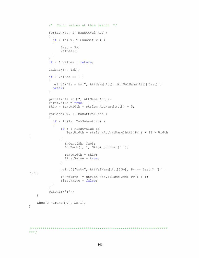
/* Count values at this branch */

ForEach(Pv, 1, MaxAttVal[Att]) {

if ( In(Pv, T->Subset[v]) ){ Last = Pv; Values++;}

} if ( ! Values ) return;

Indent(Sh, Tab);

if ( Values == 1 ) {

printf("%s = %s:", AttName[Att], AttValName[Att][Last]);break;

}

printf("%s in {", AttName[Att]); FirstValue = true; Skip = TextWidth = strlen(AttName[Att]) + 5;

ForEach(Pv, 1, MaxAttVal[Att]) {

if ( In(Pv, T->Subset[v]) ){ if ( ! FirstValue &&

TextWidth + strlen(AttValName[Att][Pv]) + 11 > Width )

{ Indent(Sh, Tab);

ForEach(i, 1, Skip) putchar(' ');

TextWidth = Skip;FirstValue = true;

}

printf("%s%c", AttValName[Att][Pv], Pv == Last ? '}' : ',');

TextWidth += strlen(AttValName[Att][Pv]) + 1; FirstValue = false;}

} putchar(':');

}

Show(T->Branch[v], Sh+1);}

/*************************************************************************/

105

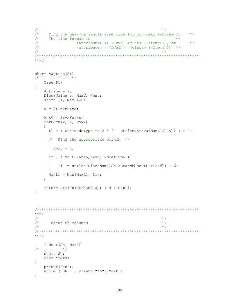
/* *//* Find the maximum single line size for non-leaf subtree St. *//* The line format is *//* <attribute> <> X.xx:[ <class (<Items>)], or *//* <attribute> = <DVal>:[ <class> (<Items>)] *//* *//*************************************************************************/

short MaxLine(St)/* -------- */ Tree St;{ Attribute a; DiscrValue v, MaxV, Next; short Ll, MaxLl=0;

a = St->Tested;

MaxV = St->Forks; ForEach(v, 1, MaxV) {

Ll = ( St->NodeType == 2 ? 4 : strlen(AttValName[a][v]) ) + 1;

/* Find the appropriate branch */

Next = v;

if ( ! St->Branch[Next]->NodeType ){ Ll += strlen(ClassName[St->Branch[Next]->Leaf]) + 6;}MaxLl = Max(MaxLl, Ll);

}

return strlen(AttName[a]) + 4 + MaxLl;}

/*************************************************************************//* *//* Indent Sh columns *//* *//*************************************************************************/

Indent(Sh, Mark)/* ------ */ short Sh; char *Mark;{ printf("\n"); while ( Sh-- ) printf("%s", Mark);}

106

/*************************************************************************//* *//* Save entire decision tree T in file with extension Extension

*//* *//*************************************************************************/

SaveTree(T, Extension)/* --------- */ Tree T; String Extension;{ static char *LastExt="";

if ( strcmp(LastExt, Extension) ) {

LastExt = Extension;

if ( TRf ) fclose(TRf);

strcpy(Fn, FileName);

if (ModelSuffix == 0) sprintf(suffixbuf,"%s",Extension);else sprintf(suffixbuf,"%s%s",ModelSuffix,Extension);

strcat(Fn, suffixbuf);#ifdef __DOS__ if ( ! ( TRf = fopen(Fn, "wb") ) ) Error(0, Fn, " for writing");

#else if ( ! ( TRf = fopen(Fn, "w") ) ) Error(0, Fn, " for writing");

#endif }

putc('\n', TRf); OutTree(T);

SaveDiscreteNames();}

/*************************************************************************//* *//* Save tree T as characters *//* *//*************************************************************************/

107

OutTree(T)/* -------- */ Tree T;{ DiscrValue v; int Bytes;

StreamOut((char *) &T->NodeType, sizeof(short)); StreamOut((char *) &T->Leaf, sizeof(ClassNo)); StreamOut((char *) &T->Items, sizeof(ItemCount)); StreamOut((char *) &T->Errors, sizeof(ItemCount)); StreamOut((char *) T->ClassDist, (MaxClass + 1) * sizeof(ItemCount));


StreamOut((char *) &T->Tested, sizeof(Attribute));StreamOut((char *) &T->Forks, sizeof(short));

switch ( T->NodeType ){ case BrDiscr:

break;

case ThreshContin:StreamOut((char *) &T->Cut, sizeof(float));StreamOut((char *) &T->Lower, sizeof(float));StreamOut((char *) &T->Upper, sizeof(float));break;

case BrSubset:Bytes = (MaxAttVal[T->Tested]>>3) + 1;ForEach(v, 1, T->Forks){ StreamOut((char *) T->Subset[v], Bytes);}break;

}

ForEach(v, 1, T->Forks){ OutTree(T->Branch[v]);}

}}

/*************************************************************************//* *//* Retrieve entire decision tree with extension Extension

*//* *//*************************************************************************/

108

Tree GetTree(Extension)/* -------- */ String Extension;{ Tree Hold, InTree(); static char *LastExt="";

if ( strcmp(LastExt, Extension) ) {

LastExt = Extension;

if ( TRf ) fclose(TRf);

if (ModelSuffix == 0) sprintf(suffixbuf,"%s",Extension);else sprintf(suffixbuf,"%s%s",ModelSuffix,Extension);

strcpy(Fn, FileName);strcat(Fn, suffixbuf);#ifdef __DOS__ if ( ! ( TRf = fopen(Fn, "rb") ) ) Error(0, Fn, "");#else if ( ! ( TRf = fopen(Fn, "r") ) ) Error(0, Fn, "");

#endif }

if ( ! TRf || getc(TRf) == EOF ) return Nil;

Hold = InTree();

RecoverDiscreteNames();

return Hold;}

/*************************************************************************//* *//* Retrieve tree from saved characters *//* *//*************************************************************************/

Tree InTree()/* ------- */{ Tree T; DiscrValue v; int Bytes;

T = (Tree) malloc(sizeof(TreeRec));

109

StreamIn((char *) &T->NodeType, sizeof(short)); StreamIn((char *) &T->Leaf, sizeof(ClassNo)); StreamIn((char *) &T->Items, sizeof(ItemCount)); StreamIn((char *) &T->Errors, sizeof(ItemCount));

T->ClassDist = (ItemCount *) calloc(MaxClass+1, sizeof(ItemCount));

StreamIn((char *) T->ClassDist, (MaxClass + 1) * sizeof(ItemCount));


StreamIn((char *) &T->Tested, sizeof(Attribute));StreamIn((char *) &T->Forks, sizeof(short));

switch ( T->NodeType ){ case BrDiscr:

break;

case ThreshContin:StreamIn((char *) &T->Cut, sizeof(float));StreamIn((char *) &T->Lower, sizeof(float));StreamIn((char *) &T->Upper, sizeof(float));break;

case BrSubset:T->Subset = (Set *) calloc(T->Forks + 1, sizeof(Set));

Bytes = (MaxAttVal[T->Tested]>>3) + 1;ForEach(v, 1, T->Forks){ T->Subset[v] = (Set) malloc(Bytes); StreamIn((char *) T->Subset[v], Bytes);}

}

T->Branch = (Tree *) calloc(T->Forks + 1, sizeof(Tree));

ForEach(v, 1, T->Forks){ T->Branch[v] = InTree();}

}

return T;}

/*************************************************************************//* *//* Stream characters to/from file TRf from/to an address *//* */

110

/*************************************************************************/

StreamOut(s, n)/* --------- */ String s; int n;{ while ( n-- ) putc(*s++, TRf);}

StreamIn(s, n)/* --------- */ String s; int n;{ while ( n-- ) *s++ = getc(TRf);}

/*************************************************************************//* *//* Free up space taken up by tree Node *//* *//*************************************************************************/

ReleaseTree(Node)/* ------- */ Tree Node;{ DiscrValue v;

if ( Node->NodeType ) {

ForEach(v, 1, Node->Forks){ ReleaseTree(Node->Branch[v]);}

free(Node->Branch);

if ( Node->NodeType == BrSubset ){ free(Node->Subset);}

} if(Node->BestAttributes)

{free(Node->BestAttributes);

111

}if (Node->BestAttributesValue){

free(Node->BestAttributesValue);}

free(Node->ClassDist); free(Node);}

/*************************************************************************//* *//* Construct a leaf in a given node *//* *//*************************************************************************/

Tree Leaf(ClassFreq, NodeClass, Cases, Errors)/* ---- */ ItemCount *ClassFreq; ClassNo NodeClass; ItemCount Cases, Errors;{ Tree Node;

Node = (Tree) calloc(1, sizeof(TreeRec)); Node->ClassDist = (ItemCount *) calloc(MaxClass+1, sizeof(ItemCount)); memcpy(Node->ClassDist, ClassFreq, (MaxClass+1) * sizeof(ItemCount)); Node->BestAttributesValue = (float *) calloc(MaxAtt+1, sizeof(float)); Node->BestAttributes=(Attribute *) calloc(MaxAtt+1, sizeof(Attribute));

Node->NodeType = 0; Node->Leaf = NodeClass; Node->Items = Cases; Node->Errors = Errors; Node->TreeSize =0;

if(Node->ClassDist==NULL||Node==NULL||Node->BestAttributesValue==NULL||Node->BestAttributes==NULL)

{printf("Not enough memory\n");exit(1);

}

return Node; }

112

/*************************************************************************//* *//* Insert branches in a node *//* *//*************************************************************************/

Sprout(Node, Branches)/* ------ */ Tree Node; DiscrValue Branches;{ Node->Forks = Branches; Node->Branch = (Tree *) calloc(Branches+1, sizeof(Tree));

}

/*************************************************************************//* *//* Count the nodes in a tree *//* *//*************************************************************************/

TreeSize(Node)/* -------- */ Tree Node;{ int Sum=0; DiscrValue v;

if ( Node->NodeType ) {

ForEach(v, 1, Node->Forks){ Sum += TreeSize(Node->Branch[v]);}

}

return Sum + 1;}

/*************************************************************************//* *//* Return a copy of tree T */

113

/* *//*************************************************************************/

Tree CopyTree(T)/* --------- */ Tree T;{ DiscrValue v; Tree New;

New = (Tree) malloc(sizeof(TreeRec));

memcpy(New, T, sizeof(TreeRec));

New->ClassDist = (ItemCount *) calloc(MaxClass+1, sizeof(ItemCount));

memcpy(New->ClassDist, T->ClassDist, (MaxClass + 1) * sizeof(ItemCount));


New->Branch = (Tree *) calloc(T->Forks + 1, sizeof(Tree));

ForEach(v, 1, T->Forks){ New->Branch[v] = CopyTree(T->Branch[v]);}

}New->BestAttributes=(Attribute *)

calloc(MaxAtt+1,sizeof(Attribute));memcpy(New->BestAttributes,T-

>BestAttributes,(MaxAtt+1)*sizeof(Attribute));New->BestAttributesValue=(float *) calloc (MaxAtt+1,sizeof

(float));memcpy(New->BestAttributesValue, T->BestAttributesValue,

(MaxAtt+1)*sizeof(float)); return New;}

/*************************************************************************//* *//* Save attribute values read with "discrete N" *//* *//*************************************************************************/

SaveDiscreteNames()

114

/* ----------------- */{ Attribute Att; DiscrValue v; int Length;


if ( SpecialStatus[Att] != DISCRETE ) continue;

StreamOut((char *) &MaxAttVal[Att], sizeof(int));

ForEach(v, 1, MaxAttVal[Att]){ Length = strlen(AttValName[Att][v]) + 1;

StreamOut((char *) &Length, sizeof(int)); StreamOut((char *) AttValName[Att][v], Length);}

}}

/*************************************************************************//* *//* Recover attribute values read with "discrete N" *//* *//*************************************************************************/

RecoverDiscreteNames()/* -------------------- */{ Attribute Att; DiscrValue v; int Length;


if ( SpecialStatus[Att] != DISCRETE ) continue;

StreamIn(&MaxAttVal[Att], sizeof(int));

ForEach(v, 1, MaxAttVal[Att]){ StreamIn(&Length, sizeof(int));

AttValName[Att][v] = (char *) malloc(Length); StreamIn(AttValName[Att][v], Length);}

}}

115

c4.5.c

#include "defns.i"#include "types.i"#include <time.h>

/* External data, described in extern.i */

short MaxAtt, MaxClass, MaxDiscrVal = 2;short IGNOREMVCLASS = 0;

unsigned int NrMVClass = 0;

ItemNo MaxItem;

Description *Item;

Boolean *AttUse;

DiscrValue *MaxAttVal;

char *SpecialStatus;

String *ClassName, *ClassAttr,

*AttName,**AttValName,

ModelSuffix = 0;FileName = "DF";

short VERBOSITY = 0,TRIALS = 10;THRESHOLD =0;

Boolean GAINRATIO = true,

SUBSET = false,BATCH = true,UNSEENS = false,PROBTHRESH = false,PRINTTREE = true,

PRUNETREE = true; chooseRandom =false;

chooseA=false; getBest=false; useFeatureSelection=false; generateReduct=false; int tempno;

Description *Reduct;

116

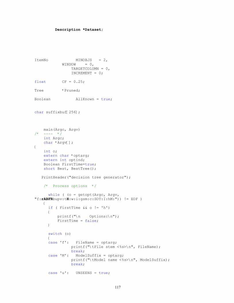
Description *Dataset;

ItemNo MINOBJS = 2,WINDOW = 0,

TARGETCOLUMN = 0, INCREMENT = 0;

float CF = 0.25;

Tree *Pruned;

Boolean AllKnown = true;

char suffixbuf[256];

main(Argc, Argv)/* ---- */ int Argc; char *Argv[];{ int o; extern char *optarg; extern int optind; Boolean FirstTime=true; short Best, BestTree();

PrintHeader("decision tree generator");

/* Process options */

while ( (o = getopt(Argc, Argv, "f:rABFRbupv:tH:w:i:gsm:c:SOT:I:hM:")) != EOF ) {

if ( FirstTime && o != 'h'){ printf("\n Options:\n"); FirstTime = false;}

switch (o){case 'f': FileName = optarg;

printf("\tFile stem <%s>\n", FileName); break;

case 'M': ModelSuffix = optarg; printf("\tModel name <%s>\n", ModelSuffix); break;

case 'u': UNSEENS = true;

117

printf("\tTrees evaluated on unseen cases\n"); break;

case 'p': PROBTHRESH = true; printf("\tProbability thresholds used\n"); break;

case 'v': VERBOSITY = atoi(optarg); printf("\tVerbosity level %d\n", VERBOSITY); break;

case 't': TRIALS = atoi(optarg); printf("\tWindowing enabled with %d trials\n", TRIALS); Check(TRIALS, 1, 10000); BATCH = false; break;

case 'w': WINDOW = atoi(optarg); printf("\tInitial window size of %d items\n", WINDOW); Check(WINDOW, 1, 1000000); BATCH = false; break;

case 'i': INCREMENT = atoi(optarg); printf("\tMaximum window increment of %d items\n",

INCREMENT); Check(INCREMENT, 1, 1000000); BATCH = false; break;

case 'g': GAINRATIO = false; printf("\tGain criterion used\n"); break;

case 's': SUBSET = true; printf("\tTests on discrete attribute groups\n"); break;

case 'm': MINOBJS = atoi(optarg); printf("\tSensible test requires 2 branches with >=%d

cases\n", MINOBJS);

Check(MINOBJS, 1, 1000000); break;

case 'c': CF = atof(optarg); printf("\tPruning confidence level %g%%\n", CF); Check(CF, 0, 100); CF /= 100; break;

case 'S': PRINTTREE = false; printf("\tSuppress printing of decision tree(s)\n"); break;

case 'O': PRUNETREE = false; printf("\tSuppress pruning (Overfit)\n"); break;

case 'T': TARGETCOLUMN = atoi(optarg); printf("\tTarget attribute in column %d\n",

TARGETCOLUMN); break;

case 'I': IGNOREMVCLASS = atoi(optarg); if (IGNOREMVCLASS == 0)

printf("\tStandard handling of MVs as class values\n");

else if (IGNOREMVCLASS == 1) printf("\tIgnore cases with MV as class value\n");

118

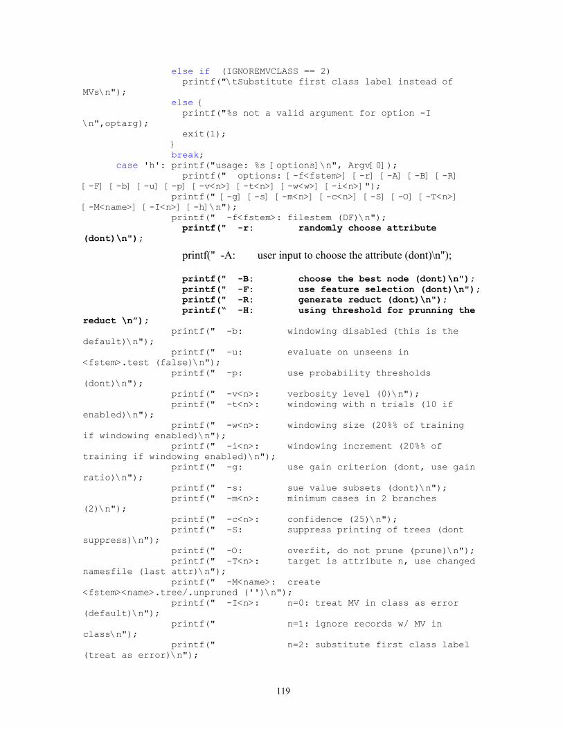
else if (IGNOREMVCLASS == 2) printf("\tSubstitute first class label instead of

MVs\n"); else { printf("%s not a valid argument for option -I

\n",optarg); exit(1); } break;

case 'h': printf("usage: %s [options]\n", Argv[0]); printf(" options: [-f<fstem>] [-r] [-A] [-B] [-R]

[-F] [-b] [-u] [-p] [-v<n>] [-t<n>] [-w<w>] [-i<n>]"); printf(" [-g] [-s] [-m<n>] [-c<n>] [-S] [-O] [-T<n>]

[-M<name>] [-I<n>] [-h]\n"); printf(" -f<fstem>: filestem (DF)\n");

printf(" -r: randomly choose attribute (dont)\n");

printf(" -A: user input to choose the attribute (dont)\n");

printf(" -B: choose the best node (dont)\n");printf(" -F: use feature selection (dont)\n");printf(" -R: generate reduct (dont)\n");printf(“ -H: using threshold for prunning the

reduct \n”); printf(" -b: windowing disabled (this is the

default)\n"); printf(" -u: evaluate on unseens in

<fstem>.test (false)\n"); printf(" -p: use probability thresholds

(dont)\n"); printf(" -v<n>: verbosity level (0)\n"); printf(" -t<n>: windowing with n trials (10 if

enabled)\n"); printf(" -w<n>: windowing size (20%% of training

if windowing enabled)\n"); printf(" -i<n>: windowing increment (20%% of

training if windowing enabled)\n"); printf(" -g: use gain criterion (dont, use gain

ratio)\n"); printf(" -s: sue value subsets (dont)\n"); printf(" -m<n>: minimum cases in 2 branches

(2)\n"); printf(" -c<n>: confidence (25)\n"); printf(" -S: suppress printing of trees (dont

suppress)\n"); printf(" -O: overfit, do not prune (prune)\n"); printf(" -T<n>: target is attribute n, use changed

namesfile (last attr)\n"); printf(" -M<name>: create

<fstem><name>.tree/.unpruned ('')\n"); printf(" -I<n>: n=0: treat MV in class as error

(default)\n"); printf(" n=1: ignore records w/ MV in

class\n"); printf(" n=2: substitute first class label

(treat as error)\n");

119

printf(" -h: show this help info\n"); exit(1); break;

case 'H': THRESHOLD = atoi(optarg); printf("\tThe threshold for prunning the reduct is

%d", THRESHOLD); break;

case 'r': chooseRandom=true; printf("\tRandomly choose attribute when there are

some attributes having the same gain ratio\n"); break;

case 'A': chooseA=true; printf("\tUser can choose the attribute when there are

some attributes having the same gain ratio\n"); break;

case 'B': getBest=true;

printf("\tGet the best Node if there are some attributes having the same gain ratio\n");

break;case 'F': useFeatureSelection=true;

printf("\t Use the Feature Selection method to mark the unnecessary attributes \n");

break;case 'R': generateReduct=true;

printf ("\t Need to generate reduct for the output of the C4.5 \n");

break;case '?': printf("\tunrecognised option (use -h for help)\n");

exit(1);}

} /* Initialise */

GetNames(); GetData(".data");

printf("\nRead %d cases (%d attributes) from %s.data\n", MaxItem+1, MaxAtt+1, FileName);

if (IGNOREMVCLASS == 1) printf("\nIgnored %d records with '?' as class label\n", NrMVClass); else if ((IGNOREMVCLASS == 2) || (NrMVClass > 0)) printf("\nReplaced '?' in %d cases with first class label\n", NrMVClass); /* Build decision trees */ if ( BATCH ) {

TRIALS = 1;OneTree();

120

Best = 0; } else {

Best = BestTree(); } scanf("%d", &tempno); exit(0);}

extern.i

/*************************************************************************//* *//* Global data for C4.5 *//* -------------------- *//* *//*************************************************************************/

extern short MaxAtt, /* max att number */MaxClass, /* max class number */MaxDiscrVal; /* max discrete values for any att

*/

extern ItemNo MaxItem; /* max data item number */

extern Description *Item; /* data items */

extern DiscrValue *MaxAttVal; /* number of values for each att */

extern char *SpecialStatus; /* special att treatment */

extern Description *Reduct;extern Boolean *AttUse;extern Description *Dataset;

extern String *ClassName, /* class names */*ClassAttr, /* Name of class atrribute */

*AttName, /* att names */ **AttValName, /* att value names */

FileName; /* family name of files */

extern Boolean AllKnown; /* true if there have been no splits on atts with missing values above the current position in the tree */

121

/*************************************************************************//* *//* Global parameters for C4.5 *//* -------------------------- *//* *//*************************************************************************/

extern short VERBOSITY, /* verbosity level (0 = none) */TRIALS; /* number of trees to be grown */

THRESHOLD; /* threshold for prunning the reduct */extern Boolean GAINRATIO, /* true=gain ratio, false=gain */

SUBSET, /* true if subset tests allowed */BATCH, /* true if windowing turned off */UNSEENS, /* true if to evaluate on test data */PROBTHRESH, /* true if to use soft thresholds */

PRUNETREE; /* true if trees should be pruned */ chooseRandom; /*true if randomly choose the attribute

if there are attributes which have the same gain info*/ chooseA; /*true if user can select attribute when

there are attributes which have the same gain info */ getBest; /*Get the best Node if there are some

attributes have the same gain info*/ generateReduct;/* true to generate the reduct for the

output of the C4.5 */ useFeatureSelection; /* true to use the Feature

selection method to mark the unnecessary attributes */

extern ItemNo MINOBJS, /* minimum items each side of a cut */

WINDOW, /* initial window size */TARGETCOLUMN, /* to be used instead of last col */INCREMENT; /* max window increment each iteration */

extern float CF; /* confidence limit for tree pruning */

types.i

/*************************************************************************//* *//* Type definitions for C4.5 *//* ------------------------- *//* *//*************************************************************************/

typedef char Boolean, *String, *Set;

typedef int ItemNo; /* data item number */typedef float ItemCount; /* count of (partial) items */

122

typedef short ClassNo, /* class number, 0..MaxClass */DiscrValue; /* discrete attribute value (0 = ?) */

typedef short Attribute; /* attribute number, 0..MaxAtt */

typedef union _attribute_value { DiscrValue _discr_val; float _cont_val; } AttValue, *Description;

#define CVal(Case,Attribute) Case[Attribute]._cont_val#define DVal(Case,Attribute) Case[Attribute]._discr_val#define Class(Case) Case[MaxAtt+1]._discr_val

#ifdef __GNUC__#include<float.h>#define Unknown FLT_MIN#else#define Unknown 1.1E-38 /* unknown value for continuous attribute */#endif

#define BrDiscr 1 /* node types: branch */#define ThreshContin 2 /* threshold cut */#define BrSubset 3 /* subset test */

typedef struct _tree_record *Tree;typedef struct _tree_record

{ short NodeType; /* 0=leaf 1=branch 2=cut 3=subset */ ClassNo Leaf; /* most frequent class at this node */ ItemCount Items, /* no of items at this node */

*ClassDist, /* class distribution of items */ Errors; /* no of errors at this node */ Attribute Tested; /* attribute referenced in test */ short Forks; /* number of branches at this node

*/ float Cut, /* threshold for continuous attribute */

Lower, /* lower limit of soft threshold */ Upper; /* upper limit ditto */

Set *Subset; /* subsets of discrete values */ Tree *Branch; /* Branch[x] = (sub)tree for outcome x */ int point;/*Shows how many attributes have the same gain info

*/ float *BestAttributesValue; /*save the best attribute value

when there are multiple attributes having the same gain info.*/ Attribute *BestAttributes; /*save the best attribute when

there are multiple attributes having the same gain info.*/ int TreeSize; /*Give the size of the tree*/ Boolean Writed;/*Show if the Node has been printed*/ }

TreeRec;

#define IGNORE 1 /* special attribute status: do not use */#define DISCRETE 2 /* ditto: collect values as data read */

123

typedef short RuleNo; /* rule number */

typedef struct TestRec *Test;

struct TestRec {

short NodeType; /* test type (see tree nodes) */ Attribute Tested; /* attribute tested */ short Forks; /* possible branches */ float Cut; /* threshold (if relevant) */ Set *Subset; /* subset (if relevant) */

};

typedef struct CondRec *Condition;

struct CondRec {

Test CondTest; /* test part of condition */ short TestValue; /* specified outcome of test */

};

typedef struct ProdRuleRec PR;

struct ProdRuleRec {

short Size; /* number of conditions */ Condition *Lhs; /* conditions themselves */ ClassNo Rhs; /* class given by rule */ float Error, /* estimated error rate */

Bits; /* bits to encode rule */ ItemNo Used, /* times rule used */

Incorrect; /* times rule incorrect */ };

typedef struct RuleSetRec RuleSet;

struct RuleSetRec {

PR *SRule; /* rules */ RuleNo SNRules, /* number of rules */

*SRuleIndex; /* ranking of rules */ ClassNo SDefaultClass; /* default class for this ruleset */

};

Appendix B – Data set of Monk3 Sample

Monk3.names

0, 1 |classes

124

attribute#1 : 1, 2, 3


attribute#3 : 1, 2


attribute#5 : 1, 2, 3, 4

attribute#6 : 1, 2

monk3.data

1,1,1,1,1,2,11,1,1,1,2,1,11,1,1,1,2,2,11,1,1,1,3,1,01,1,1,1,4,1,01,1,1,2,1,1,11,1,1,2,2,2,11,1,1,2,4,2,01,1,2,1,2,2,11,1,2,1,4,2,01,1,2,2,2,2,11,1,2,2,4,1,01,1,2,2,4,2,01,1,2,3,1,1,11,1,2,3,1,2,11,1,2,3,3,1,11,1,2,3,3,2,11,2,1,1,3,1,11,2,1,2,2,1,11,2,1,2,2,2,11,2,1,2,3,1,01,2,1,3,1,1,11,2,1,3,1,2,11,2,1,3,2,1,11,2,1,3,2,2,11,2,1,3,3,2,11,2,1,3,4,1,01,2,2,1,3,1,11,2,2,1,4,2,01,2,2,2,1,1,11,2,2,2,2,1,11,2,2,2,2,2,11,2,2,3,1,1,11,2,2,3,2,1,11,2,2,3,2,2,11,3,1,1,2,1,01,3,1,1,4,1,0

125

1,3,1,2,3,2,01,3,1,2,4,1,01,3,1,3,1,1,01,3,1,3,3,1,01,3,2,1,1,1,01,3,2,1,1,2,01,3,2,1,2,1,01,3,2,1,4,2,01,3,2,2,3,2,01,3,2,2,4,2,01,3,2,3,4,1,02,1,1,1,1,1,12,1,1,1,1,2,12,1,1,1,4,1,02,1,1,1,4,2,02,1,1,2,1,1,12,1,1,2,1,2,12,1,1,3,2,2,12,1,1,3,3,2,12,1,1,3,4,1,02,1,2,1,2,2,12,1,2,2,4,1,02,1,2,3,1,2,12,2,1,1,3,2,12,2,1,1,4,2,02,2,1,2,1,2,12,2,1,2,2,1,02,2,1,3,1,1,12,2,1,3,2,2,12,2,1,3,3,1,02,2,1,3,3,2,02,2,1,3,4,2,02,2,2,1,2,2,12,2,2,2,1,2,12,2,2,2,3,1,12,2,2,2,3,2,12,2,2,3,4,1,02,3,1,1,3,1,12,3,1,2,1,1,02,3,1,2,2,1,02,3,1,2,2,2,02,3,1,2,3,2,02,3,1,3,3,1,02,3,2,1,1,2,02,3,2,1,2,2,02,3,2,1,4,1,02,3,2,2,3,1,02,3,2,2,4,2,02,3,2,3,1,1,02,3,2,3,2,1,02,3,2,3,4,2,03,1,1,1,1,1,13,1,1,1,2,1,13,1,1,1,3,1,13,1,1,2,4,2,03,1,1,3,1,2,1

126

3,1,1,3,4,2,03,1,2,1,2,1,13,1,2,2,3,2,13,1,2,2,4,2,03,1,2,3,1,1,13,2,1,1,2,2,13,2,1,1,4,1,03,2,1,2,3,1,13,2,1,3,1,2,13,2,2,1,2,2,13,2,2,1,3,2,13,2,2,2,1,2,13,2,2,3,1,1,13,2,2,3,3,2,13,2,2,3,4,1,03,3,1,1,3,2,13,3,1,1,4,1,13,3,1,2,4,2,03,3,1,3,1,1,03,3,1,3,2,1,03,3,1,3,2,2,03,3,1,3,4,1,03,3,2,1,1,1,03,3,2,1,1,2,03,3,2,2,2,2,03,3,2,2,3,2,03,3,2,3,1,1,03,3,2,3,3,2,03,3,2,3,4,2,0

127

Documents

Finding Optimal Reduct for Rough Sets by Using a Decision