Embed Size (px)
Citation preview

RESPONSE TIME EVALUATION OF REAL-TIME
SENSOR BASED VARIABLE RATE TECHNOLOGY
EQUIPMENT
By
PRAVEEN J BENNUR
Masters of Science in Biosystems & Agricultural
Engineering
Oklahoma State University
Stillwater, Oklahoma
2009
Submitted to the Faculty of the Graduate College of the
Oklahoma State University in partial fulfillment of the requirements for
the Degree of MASTER OF SCIENCE
July, 2009

ii
RESPONSE TIME EVALUATION OF REAL-TIME
SENSOR BASED VARIABLE RATE TECHNOLOGY
EQUIPMENT
Thesis Approved:
Dr. Randy Taylor
Thesis Adviser
Dr. John Solie
Dr. Paul Weckler
Dr. Ning Wang
Dr. A. Gordon Emslie
Dean of the Graduate College

iii
ACKNOWLEDGMENTS
First and foremost I offer my sincerest gratitude to my advisor and supervisor, Prof. Dr.
Randy Taylor, who has supported me throughout my research for his patience,
motivation, enthusiasm, and immense knowledge whilst allowing me the room to work in
my own way. His invaluable guidance has helped me during the entire duration of my
research and writing of this thesis. I attribute the level of my Masters degree to his
encouragement and effort. My deepest gratitude also goes to the members of my
supervisory committee, Prof. Dr. John Solie, Assoc Prof. Dr. Paul Weckler and Asst Prof.
Dr. Ning Wang for their continuous encouragement and insightful comments. My sincere
thanks go to Emeritus Prof. Dr. Marvin Stone for his invaluable and much needed advice
throughout my day to day research activity. My special thanks to under graduate student
Kyle Hiner, laboratory supervisor Wayne Kiner and his team and to the Department of
Biosystems and Agricultural Engineering for providing me the support and equipment I
needed for my research. Last but not the least, I wish to express my love and gratitude to
my beloved family for their understanding, endless love and blessings throughout my life.

iv
TABLE OF CONTENTS Chapter Page
INTRODUCTION .............................................................................................................. 1
1.1 Precision Agriculture ................................................................................................ 1
1.2 Variable Rate Technology (VRT) ............................................................................. 2
REVIEW OF LITERATURE ............................................................................................. 4
2.1 Standards for Evaluating Variable Rate Technology Equipment ............................. 4
2.2 Factors Affecting Lag-Time of Inline Injection Sprayers ......................................... 5
2.3 Lag-Time and Charge-Time of Inline Injection Sprayers......................................... 6
2.4 Static and Dynamic Response Time of Variable Rate Controllers ........................... 7
2.5 Time-Delay in Pressure Based Variable Rate Application ....................................... 9
2.6 Variable Rate Technology in Agricultural Applications ........................................ 10
2.7 Dynamic Performance Benchmarking in VRT Equipment .................................... 12
2.8 Research Focus ....................................................................................................... 14
2.9 Research Objective ................................................................................................. 17
MATERIALS & METHODS ........................................................................................... 18
3.1 VRT System Components....................................................................................... 18
3.2 Raven SCS 440 Rate Controller ............................................................................. 22 3.3 PWM-Applicator (PWM Control with fixed orifice nozzles) .............................. 223 3.4 FC-Applicator (FC Valve with variable orifice nozzles) ........................................ 26
3.5 Data Acquisition System......................................................................................... 28
3.5.1 Hardware .......................................................................................................... 29
3.5.2 Software ........................................................................................................... 30
3.6 Rate Controller Inputs ............................................................................................. 33
3.7 Data Collection ....................................................................................................... 34
3.8 Overall Response Time Measurement .................................................................... 35
RESULTS & DISCUSSION............................................................................................. 38
4.1 Controller Response Time for PWM-Applicator System for Step Input ................ 38
4.2 Controller Response Time for PWM-Applicator System for VRT Input ............... 41

v
4.3 Controller Response Time for FC-Applicator System for Step Input .................... 46
4.4 Controller Response Time for FC-Applicator System for VRT Input ................... 49
4.5 Controller Response Time Comparison .................................................................. 53
4.6 Boom Pressures in PWM-Applicator System ......................................................... 55
4.7 Boom Pressures in FC-Applicator System ............................................................. 56
CONCLUSION ................................................................................................................. 58
FUTURE WORK .............................................................................................................. 60
REFERENCES ................................................................................................................. 61
APPENDICES .................................................................................................................. 63
Appendix A: Front Panel of LabVIEW Data Acquisition Program ............................. 63
Appendix B: Block Diagram of LabVIEW Data Acquisition Program ....................... 64
Appendix C: Wiring Diagram of NI USB-6210 Data Acquisition System .................. 65
Appendix D: Raven Controller Rate Change Command Serial Data Format .............. 66
Appendix E: PIC Program for Simulating MAP Based Step Input .............................. 67
Appendix F: PIC Program for Simulating Sensor Based Variable Rate Input ............. 68
Appendix G: MATLAB Program for frequency analysis using FFT ........................... 70

vi
LIST OF TABLES
Table Page Table 1 Controller response time for PWM-Applicator system for step input ................. 38
Table 2 Controller response time for PWM-Applicator system for variable rate input ... 42 Table 3 Controller response time for FC-Applicator system for step input ..................... 46
Table 4 Controller response time for FC-Applicator system for variable rate input ........ 49 Table 5 Minimum controller response time for PWM-Applicator and FC-Applicator .... 53

vii
LIST OF FIGURES
Figure Page Figure 1 Raven SCS-440 Application Rate Controller ..................................................... 18
Figure 2 StreamJet SJ3-04 TeeJet Fixed Orifice Nozzle and Capstan solenoid valve ..... 19 Figure 3 Raven Fast Close (FC) Valve ............................................................................. 20
Figure 4 TurboDrop Variable Rate TDVR02 Variable Orifice Nozzle ............................ 20
Figure 5 Raven Flow Meter RFM 60P ............................................................................. 21
Figure 6 Raven - Pressure Transducer .............................................................................. 21
Figure 7 PWM-Applicator (Capstan PWM control with TeeJet fixed orifice nozzles) ... 25 Figure 8 FC-Applicator (Raven FC Valve with TurboDrop variable orifice nozzles) ..... 27 Figure 9 USB 6210 Data Acquisition System .................................................................. 29
Figure 10 (a) Blancett Flow Meter (b) MSP300 Pressure Transducer ............................. 30
Figure 11 RS 232 Serial port data tap ............................................................................... 31
Figure 12 USB 6210 Data Acquisition System with FC-Applicator VRT system ........... 32
Figure 13 Overall response time measurement with FC-Applicator VRT System .......... 37 Figure 14 Controller response for step input to PWM-Applicator ................................... 39
Figure 15 Controller response time with 5 point moving average.................................... 41
Figure 16 Controller response for VR input PWM-Applicator ........................................ 44
Figure 17 Actual v.s. set point rate for VR input to PWM-Applicator ............................. 45
Figure 18 Actual v.s. set point rate with 0.5 s lag for VRinput to PWM-Applicator ....... 45
Figure 19 Controller response for step input to FC-Applicator ........................................ 47
Figure 20 Oscillating controller response for FC-Applicator step input .......................... 48
Figure 21 Controller response for VR input to FC-Applicator ........................................ 51
Figure 22 Actual v.s. set point rate for VR input to FC-Applicator ................................ 52
Figure 23 Actual v.s. set point rate with 0.6 s lag for VR input to FC-Applicator ........... 52
Figure 24 Boom pressures in PWM-Applicator system ................................................... 55
Figure 25 Boom pressures in FC-Applicator system ........................................................ 56

1
CHAPTER I
INTRODUCTION
1.1 Precision Agriculture
Precision agriculture among agricultural producers has been growing over the past
decade as producers have realized benefits with regard to increased profitability and
reduced environmental impact. Studies of economic feasibility and analysis of using
precision farming equipment have revealed that the benefits obtained from precision
agriculture adoption have mostly out weighted the initial investment and maintenance on
the precision agriculture equipment (Godwin et al., 2002). For instance, numerous studies
have been conducted to improve the use efficiency of nitrogen as a fertilizer in cereal
production. The driving factors for these studies were that (1) nitrogen fertilizer prices
have doubled over the past few years and (2) environmental impact of excess or
misapplied nitrogen fertilizer on cereal crops. According to Raun et al. (1999), a one
percent increase in the nitrogen use efficiency in cereal production worldwide would save
around $234,658,462 in nitrogen fertilizer costs. Owing to this saving potential,
agricultural producers are interested in adopting variable rate technology in their farming
practice. Moreover, Solie et al. (1996) suggested that nitrogen application using variable
rate technology should treat the field area in the elemental size of not greater than 1.96
m2 to reap the benefits of variable rate nitrogen application technology. This puts forth a
lot of questions and expectations from commercially available variable rate technology

2
equipment such as: “Is the equipment capable of providing enough resolution for
applying nitrogen at variable rates and at different tractor speeds and / or with different
spatial variability in agricultural fields? What are the costs involved and is it affordable?
What are the different components involved in variable rate technology? How can the
performance of each of the component be evaluated? What is the effect of combining
these components on the overall system performance? Are there any standards defined to
evaluate the variable rate technology and its associated equipment?” To answer these
questions and to see if the expectations are met, much research has been done over the
past decade on different aspects and applications of variable rate technology. An
overview of relevant research done in this field of variable rate technology and their
findings is in the review of literature section.
1.2 Variable Rate Technology (VRT)
Variable rate fertilizer application can be of three types: geographic information system
(GIS) map-based or real time sensor-based or a combination of map and sensor-based.
GIS map-based variable rate application is used where application amounts and rates are
predetermined based on the historic spatial data such as yield and/or soils maps. The field
is divided into sections and application rates are fixed for each section in the field. Map-
based VRT system uses a predefined application map (prescription map) to change the
application rate and rate changes are less often. To achieve variable rate application,
position coordinates are needed in map-based VRT. In contrast, in the case of sensor-
based and combination variable rate application methods, the input comes from a sensor
that triggers a change in application rate in real time. In most cases, this application rate

3
change is triggered every second. Plant or soil sensors are needed in a sensor based VRT.
Both the systems need a flow sensor for fertilizer rate, a ground speed sensor, a rate
controller, and actuator valves/motors. Application rate is adjusted by a variable rate
controller, which is at the heart of the VRT system. VRT controllers incorporate
embedded microcontrollers that accept sensor inputs, GIS prescription data, customized
user commands through hardware and software interface and calculate the required
application rate using a formula or an algorithm. The calculated rate is then translated
into actual fertilizer output through actuators, often via motor controlled flow control
valves or solenoid controlled nozzles.
Rate controllers are available commercially that interface with different devices using
standard connectors. Important criteria when selecting rate controller or a VRT control
system is the response time. A fast responding VRT system is needed to make quick rate
changes while the applicator moves across the field. A map based VRT system needs a
programmable look ahead feature capable of providing predictive speed compensation
that is essential for synchronizing fertilizer rates with changing tractor speeds after
subtracting inherent system lag times. Sensor based VRT provide up-to-date information
at the time of the application and the components need to be very fast in order to catch up
to the rate change commands that come every second. The information from the sensors
is fed to the VRT controllers in real time and the lag time of sensor based VRT system
needs to be very small.
4
CHAPTER II
REVIEW OF LITERATURE
2.1 Standards for Evaluating Variable Rate Technology Equipment
Determining the key factors for development of a standard test for evaluating the variable
rate technology and its equipment has been done by Shearer et al. (2002) where in, they
have reviewed an existing set of standards in the ASABE framework which have an
impact on variable rate technology. They found that three existing ASABE standards can
be used to evaluate a variable rate technology product with slight tailoring needed to
accommodate for variable application rates. The three standards evaluated were:
1. ASABE S341.3 Feb1999 - Procedure for measuring distribution uniformity and
calibrating granular broadcast spreaders.
2. ASABE EP371.1 - Jan 2001 - Procedure for calibrating granular applicators.
3. ASABE EP367.2 - Jan 2002 - Guide for preparing field sprayer calibration.
Shearer et al’s (2002) evaluations showed that the test standards should be based on the
controller response against the product distribution and that a set of procedures to
evaluate the controller response was not available. Shearer et al. (2002) also suggested
that for addressing the issue of product distribution, or more so, the inherent delay in

5
some application systems, the ASABE standards mentioned above needed revision to
accommodate evaluating the quality for application rate changes in different precision
farming areas. Moreover, these standards were for steady state systems. Shearer et al.
(2002) suggested that one approach to evaluate granular application would be to specify a
2D collection pan arrangement for measure changes in the application rates and criteria
for evaluating the transport lags from the point of metering the grain to the actual
application device. This review suggests that the delay times of different components of a
variable rate system are to be accommodated and based on this, test standards need to be
developed for different variable rate technology applications.
2.2 Factors Affecting Lag-Time of Inline Injection Sprayers
Researchers in the field of precision agriculture and more specifically in the field of
variable rate technology application have tried to evaluate individual components of the
commercially available variable rate technology equipment. The evaluation was based on
performance, response time, dynamic characteristics and lag time. Some researchers have
benchmarked different commercial available variable rate controllers and associated
components. Zhu et al. (1997) investigated the factors affecting the lag times of inline
injection sprayer systems for one boom section. The factors considered for investigation
were the total number of active spray nozzles, size of the boom, changes in ground speed,
and the product viscosity. They used different liquids with viscosities in ranging from 1
to 98 mPa s. Most pesticides have viscosities within this range. Pesticide injection
occurred at the center of the boom and was regulated by a Raven SCS 700 rate controller
depending on the desired application rate and ground speed. The effluxes from spray

6
nozzles were collected and the concentrations were measured to determine change in
concentrations at different nozzle locations on the boom section. The tests were
conducted for two boom section diameters of 1.1 and 2.1 cm, different pesticides
viscosities, and different number of active nozzles. For every test, two measurements
were made by fixing a particular set of active nozzles, fixed boom section diameter, and
fixed pesticide viscosity. The first measurement was made when the ground speed
changed from 1.6 to 6.4 km/hr in 5 s and the second measurement was made when the
ground speed changed from 6.4 to 1.6 km/hr in 5 s. These measurements were made to
determine the influence of speed variation on lag times. Zhu et al. (1997) found that
viscosity plays a very minor role and does not affect the lag time much though there were
changes in travel speed, where as the cross sectional diameter of the boom had a great
impact on the lag time for the end nozzle in the boom. There was a two fold increase in
lag time for a two fold increase in diameter. This lag time was significantly higher than
the lag time measured by changing the tractor speed from either 1.6 to 6.4 km/hr in 5 s or
6.4 to 1.6 km/hr in 5 s.
2.3 Lag-Time and Charge-Time of Inline Injection Sprayers
In another study, Sumner et al. (2000) said that for variable rate technology to be
successful for pesticide application, lag and charge times of injection sprayers would be
important criteria. He defined the lag time as the time between the time of injection of the
chemical and the time it reaches the nozzle and the charge time as the extra time required
by the chemical at the nozzle to reach a desired concentration. To measure these times,
Sumner et al. (2000) developed and used a string collector system and measured the lag

7
and charge times for two spray booms. This system used strings to collect the dye which
was sprayed from one nozzle of the boom section. The distribution of the dye on the
string was captured and analyzed by a commercially available string analysis system and
software to determine the lag and charge times. The lag time ranged from 0.2 s to 4.6 s
for a one nozzle to eight nozzle boom and charge time ranged from 0.2 s to 0.9 s for the
same nozzle range. The lag time and the charge time did not vary much with changes in
flow rate, but increased with the number of nozzles in the boom section. The reason for
wide range of measured value for lag and charge times were change in number of nozzles
in the boom. The measured lag times using the string collector system had similar values
as compared to the theoretically estimated lag times which used flow rate and volume for
calculating the lag time, thereby establishing the credibility of string collector system for
measuring lag and charge times. This study showed that as the injection system is close to
the nozzle and if the flow rates are high enough, then there would be less lag. The focus
of these studies was on the delay involved in injection sprayer systems but did not
address variable rate technology equipment used for changing rates of the total volume
applied. These delays are inherent in the variable rate controller itself.
2.4 Static and Dynamic Response Time of Variable Rate Controllers
Yang (2000) studied a commercially available variable rate controller and found
interesting results with respect to the static and dynamic response times when being used
for a variable rate application for two liquid fertilizers. He used a FALCON controller
system along with the other variable rate application equipment. This controller provided
feasibility to tune proportional, integral and derivative parameters to get optimal initial
8
and steady state responses for a desired change in the input rate. Once the parameters
were fixed, response time was measured for different application rates and priming
conditions. Here, priming is a preparation process that involves cleaning and running the
system with the same liquid chemical and at desired flow rate before it could be used for
collecting data with actual experiments there by reducing measurement errors. Priming
with desired application rate was done before each test that needed a change in
application rate. Tests were done with different application rate changes from 0 to 150
l/ha, 0 to 300 l/ha and 0 to 450 l/ha. With each change in application rate, the system was
primed to the desired rate before the test. The dynamic response time of the controller
was around 0.5 s and the controller took around 2 s to stabilize at the required rate. In
another test, the target rate was fixed to 360 l/ha and the priming was done at different
levels for each test. Yang (2000), observed that when the priming rate was above the
desired rate, the overshoot was almost 100% and the time taken for stabilizing was 4.5 s
as compared to 1 s when the priming rate and the desired rates were almost same. For a
test where the priming rate was 240 l/ha and application rate changed from 240 l/ha to
480 l/ha, the rise-time increased proportionally between 1 s to 4.5 s but with no
overshoot. In a similar test, where the priming was done at 480 l/ha and the rate varied
from 480 l/ha to 240 l/ha, it was seen that there were large overshoots and it took a lot of
time to stabilize at the desired rate when it was low. Yang (2000) observed that, in
general there was a 1 s delay when a rate changed and remained constant for 4 s,
irrespective of whether the rate was changing in the upward or downward direction. All
the tests indicated that the dynamic controller response time delay was around 1s.
Additionally, Yang (2000) also observed that the delay in GPS positioning did have an
9
effect on the application accuracy in case of map based prescribed variable rate
application.
2.5 Time-Delay in Pressure Based Variable Rate Application
As discussed earlier the application accuracy of variable rate technology equipment could
depend on the GPS response time and its accuracy. Much research has been done to
determine the effect of inherent delays in GPS and the delays in flow control valves used
for variable rate application. The main aim of the research was to find the quantitative
error between the desired and actual application rates. According to Anglund and Ayers
(2002), the agricultural industry’s use of variable rate technology is ahead of scientific
research and that there exists no verification of the accuracy of the variable rate
technology system as a whole. Much field research has been done to determine the yield
differences with and without use of variable rate technology equipment under the
assumption that variable rate technology equipment works properly. Anglund and Ayers
(2002) found that there was a need for an extensive performance testing of a variable rate
sprayer system with respect to the spraying amount and location which could lead to
standard test procedures for evaluating commercially available variable rate sprayer
system. Anglund and Ayer (2002) found that in the case of pressure based variable rate
application of liquid chemicals; there was an average of 0.5 s GPS lag and around 1.5 s of
control valve lag. So a total of 2 s lag was compensated by a pre-programmed “look-
ahead” time in the controller in case of map based variable rate technology equipment.
Anglund and Ayer (2002) conducted field tests of commercially available variable rate
technology equipment consisting of a Raven SCS 750 spray controller, a control program

10
from MapInfo Corp to determine the desired application rate based on a map and current
position, a Trimble AgGPS 132 GPS receiver, a Raven speed sensor, and a Raven RFM
200 flow meter as controller sensor inputs. They used a Campbell Scientific 2X micro-
logger to log the data from sensors which indicated the change in application rates at
different times and positions. The GPS position data and the logged data from the
Campbell Scientific 2X micro-logger were brought to a common time base and analyzed.
The analysis found that the application rates were within 2.25% of the desired rates
which is reasonable. The delay involved in GPS was around 0.5 s and the delay because
of the control valve was 1.5 s. The software used allowed for the setting of a “look-
ahead” time for compensating the delays involved. This compensation would be
reasonable if the same components were used to build the variable rate technology
equipment. Practically this would not be possible to effectively use variable rate
technology equipment if the compensation time has to be found and set by conducting
experiments for each variable rate controller. Moreover, the idea of a “look-ahead” time
makes sense only if it is a map based variable rate application. In real-time sensor based
variable rate application, the concept of “look-ahead” time compensation cannot be used
though one could place the sensors ahead of application point. Though the GPS time lag
would not exist in these systems the demand for a control valve with a low response time
is real so that the application errors are within reasonable limits.
2.6 Variable Rate Technology in Agricultural Applications
Variable rate technology equipment and variable rate application is being practiced in
different agricultural fields. Some of the common agricultural areas where variable rate

11
technology application is being used, are in granular fertilizer applications using spinner
spreaders and pneumatic applicators, liquid chemical and fertilizer application, site
specific weed management application, and variable rate single tree fertilizer application
for citrus groves. Researchers have developed different techniques to evaluate and find
the response time of rate controllers in different agricultural applications. Sui et al. (2003)
developed an optical method to determine the time delay of spray system used in the field
of variable rate liquid chemical application, where three different chemicals were being
applied at different rates at the same time. To simulate this situation, three different
colored dyes were used for application. The dye solution flowing out of the nozzles
during the tests were collected into 10 ml cuvettes. Spectral analysis was done to
determine the concentration of the dyes obtained from different nozzles. The
concentrations of the dyes were related to the time required for the dyes to reach the
nozzles when the flow rate changed.
In another application, Fulton et al. (2005) studied the rate response of the variable rate
technology equipment for granular application. They used two spinner disc spreaders and
two pneumatic applicators. Each applicator was fitted with different controllers and
drives. Pan tests were conducted in the field using the modified ASABE standard S341.2
test protocol for variable rate application using the variable rate technology equipment.
Different variable rate technology equipment yielded different results and different
response times. Fulton et al. (2005) observed that in case of granular applications, there
were cases where the rate transition times were quite high which in turn dictated the
spatial resolution. Fulton et al. (2005) predicted that higher ground speed could be an

12
issue in case of granular applications and should be reduced to reduce application errors.
Because of the variable response times in different applicators tested, and with varying
agricultural applications using the variable rate technology equipment, Fulton et al.
(2005) suggested that the manufacturers of the variable rate technology equipment
specify the transition and delay times to the end users. This also highlighted the need for
having a standard procedure for determining and specifying these values.
2.7 Dynamic Performance Benchmarking in VRT Equipment
The research experiment results from Anglund and Ayer (2002) showed that the time
delays for components in a variable rate technology system are different. A majority of
the delay was caused by the control valve which was around 1.5 s as measured by
Anglund and Ayer (2002) in their application. Over time, researchers became interested
in studying the technology used in the existing variable rate technology equipment and to
see if the components used were optimal for the application. Numerous studies and
benchmarking of components used in variable rate technology equipment were made.
One study on the butterfly control valves used in the variable rate technology equipment
is of particular interest. Cugati et al. (2006) conducted a research on the steady state
response and the dynamic response of two different types of control valves used with
commercially available variable rate technology equipment. One of the control valves
was a hydraulic flow control valve which was DC motor driven and the other was a
solenoid flow control valve. These valves were used for tests in the variable rate
technology equipment used for variable rate application in citrus groves. Cugati et al.
(2006) concluded that the dynamic behavior of the valves and other components in the

13
variable rate technology equipment had a very high impact on the performance and
accuracy of the variable rate technology equipment thus affecting the spread pattern of
the granular fertilizer on citrus groves. Cugati et al. (2006) experiments measured the
steady state response times and the dynamic response time for the two types of valves
selected. The DC motor controlled valve was rotated to a pre-determined angle of 1.5
degrees by applying a voltage to the DC motor and the flow rate changes were recorded.
Tests were repeated for different angles or valve positions. Similar tests were performed
on the solenoid control valve. The results showed that the steady state behavior for both
valves was linear, but there was no flow observed from the starting point of 0 degree to 3
degree angle in case of the DC motor controlled valve. It was also observed that the
hysteresis of the DC motor controlled valve was higher than that of the solenoid valve.
With the data acquired from the experiments, the time delay was calculated for both the
control valves. This time delay was the time from issuing a rate change command to the
time when the flow rate changed because of the movement of the valve. For both the
valves, the dynamic behavior was linear. The response for both valves was modeled as a
first order transfer function. Interestingly, the delay time and the time constant measured
for both the valves were different. The delay time and the time constant in case of the DC
motor controlled control valve were 0.08 s and 0.04 s respectively whereas the delay time
and the time constant in case of the solenoid valve were 0.04 s and 0.02 s respectively.
Cugati et al. (2006) suggested that the valve with smaller time constant and smaller delay
time would aid in a better closed loop control and thus suggested that use of solenoid
control valve was better than the DC motor controlled valve in case of a variable rate
application system.

14
Another experiment conducted by Cugati et al. (2006) tried to benchmark the dynamic
performance of a commercially available variable rate controller and associated
components for variable rate fertilizer application in citrus groves. The bench-marking as
done earlier with respect to two different types of commercially available valves, was
repeated with the other components of the variable rate equipment. In his experiments,
the triggering modes of variable rate technology equipment were changed for a desired
rate change and the dynamic performance was evaluated. Cugati et al. (2006) found that
the performance of the variable rate technology equipment triggered by real-time sensors
was better as compared to the variable rate technology equipment triggered by GPS. This
implied that the GPS delay does affect the dynamic performance of the variable rate
technology equipment. With all these results, Cugati et al. (2006) concluded that the
selection of components that are used to build variable rate technology system have an
impact on the overall performance of the variable rate technology equipment. From the
experimental results, Cugati et al. (2006) concluded that the variable rate technology
equipment which had solenoid valve for flow control, a high resolution encoder and a
system triggered by real-time sensors for a rate change had the best overall performance
in the variable rate application and in particular for variable rate application for citrus
groves.
2.8 Research Focus
As technology advances faster than ever, so do the applications based on these
technologies. The present commercially available variable rate technology equipment is
complex with many different components. Moreover, the functioning of each of the

15
components depends on the response of other components or to be more specific the
“response time” of the other components. This ultimately determines the ability of
variable rate technology equipment to perform at the desired scale. Typically a variable
rate application system is based on a sensor input or based on a prescription map. This
involves various components of the variable rate technology equipment like plant vigor
sensors, flow sensors, pressure transducers, GPS sensors, ground speed sensors, wiring
harness, rate controller, flow control valves, injection sprayers, junction box / interface
modules, console / virtual terminal, on-board computer running the control program etc.
All of the components involved operate on the inputs from the other. This means that
there is a high level of interdependency among the components and that there is a time
delay involved due to the inherent characteristic of the component, time delay due to the
dependency on the other component or because of certain other limitations. Much
research has been done to determine the response times of individual components that
make up the variable rate technology equipment. That is, individual research on injection
sprayers, flow control valves and to a certain extent on rate-controllers in different areas
of variable rate technology applications has been conducted. There have been no specific
studies or measurements done in the area of application of liquid nitrogen fertilizer using
commercially available real time sensor based variable rate technology equipment.
Moreover, not much research has been done to measure the delay involved in each of the
individual components and also the overall VRT system, especially when all the
individual components of VRT system work together to achieve a real time variable rate
application as desired, with set spatial resolution. Owing to the enormous saving potential
both economically and environmentally with regard to the efficient use of nitrogen as a

16
fertilizer, the performance expectation and demand on variable rate technology
equipment used for nitrogen application becomes extremely important.
As seen in previous sections, one of the important factors affecting performance of
variable rate technology equipment used for nitrogen application is the response time.
Measuring the response time of variable rate technology equipment used for nitrogen
application involves, measuring individual delay times which add up to the overall
response time of the variable rate equipment, starting from the time when real time sensor
senses a change in plant characteristics to the time when change in rate is actually
achieved. This involves measuring:
1. Time between a change in sensor signal (which demands a rate change) and the
time it takes to reach the program running on an on-board computer responsible
for triggering a rate change.
2. Time taken by the on-board computer program to trigger the rate controller for a
desired rate change.
3. Time required by the rate controller to change the desired flow rate.
4. Time required for the actual flow rate to match the desired flow rate.

17
Time required by the rate controller to change to the desired flow rate depends on type of
controller and options available on the controller to change control speed or response
time of the controller itself. Depending on the measured total response time of the
variable rate technology equipment, it is possible to determine if this time is small
enough to satisfy the set spatial resolution for variable rate nitrogen application in turn
determining the maximum application speed.
2.9 Research Objective
The objectives of this research are:
1. To measure the response time of a commercially available rate controller with two
different control valve configurations: pulse width modulated technology with
fixed orifice nozzles and a fast-close valve with variable orifice nozzles.
2. To determine the optimum rate-controller parameter setting that results in a
minimum response time for the two applicator configurations.
3. To measure overall response time for the two applicator configurations using the
determined optimum controller setting when used in a sensor based VRT system.

18
CHAPTER III
MATERIALS & METHODS
3.1 VRT System Components
A VRT system consists of several different components like flow sensors, ground speed
sensors, hand-held computer that converts sensor value to fertilizer application rate, rate
controller, pressure transducers, spray nozzles, etc with the application rate controller
being at the heart of VRT system.
A test sprayer was equipped with a VRT system using two different applicator
configurations at different times. A Raven SCS 440 (Raven Industries, Sioux Falls, SD)
rate controller (figure 1) was used to control rate changes to the applicator systems.
Figure 1 Raven SCS-440 application rate controller console.

19
Two different applicator configurations were used on the test sprayer to determine
performance by measuring response time. The first applicator configuration (PWM-
Applicator) consisted of a Synchro System (Capstan Ag Systems, Topeka, KS) pulse
width modulation (PWM) flow technology that adjusted nozzle solenoid duty cycle with
fixed orifice nozzles (StreamJet SJ3-04, TeeJet Spraying Systems Company, Wheaton,
IL) (figure 2).
Figure 2 TeeJet StreamJet SJ3-04 fixed orifice nozzle and Capstan solenoid valve.
The second applicator configuration (FC-Applicator) consisted of a fast close (FC) valve
(Raven Industries, Sioux Falls, SD - P/N 1-063-0172-170) (figure 3) with variable orifice
nozzles (TurboDrop Variable Rate – TDVR02, GreenLeaf Technologies; Covington, LA)
(figure 4).

20
Figure 3 Raven fast close (FC) valve.
Figure 4 TurboDrop TDVR02 variable orifice nozzle (yellow) for metering with an
oversized StreamJet nozzle (blue) to generate a pattern.

21
The system had a RFM 60P (1-60 GPM Poly) flow-meter (Raven Industries Inc, Sioux
Falls, SD – P/N 1-063-0171-793) (figure 5) to measure flow in the boom and provide
feedback to rate controller.
Figure 5 Raven flow meter RFM 60P.
An optional pressure transducer from Raven (Raven Industries Inc, Sioux Falls, ND)
(figure 6) with range of 0 to 700 kPa (0-100 psi) measured the pressure in the boom for
display on rate controller console.
Figure 6 Raven pressure transducer.
22
3.2 Raven SCS 440 Rate Controller
A Raven SCS 440 rate controller (Raven Industries Inc, Sioux Falls, SD) was selected for
performance evaluation (figure 1). It provided precise automatic rate control and could be
pre-programmed with two separate application rates as well as accept application rates
from a serial input (Raven Part #: 016-0159-822). The Raven controller used four
parameters of control valve that directly affected response time called VALVCAL
number consisting of 4 digits. Parameters that could be controlled by changing the digits
were:
Digit1: Valve Backlash – Controls the time of the first correction pulse after a change in
the correction direction is detected. Range: 1 to 9 (1 – Short Pulse, 9 – Long Pulse).
Digit2: Valve Speed – Controls the response time of control valve motor. Range: 0 to 9
(0 – Fast, 9 – Slow for FC Valve and 0 – Slow, 9 – Fast for Standard Valve).
Digit3: Brake Point – Sets the point at which control valve motor begins braking, so as
not to over shoot the desired rate. The digit is the percent away from the target rate.
Range: 0 to 9 (0 = 5%, 1 = 10%, 9 = 90%).
Digit4: Dead Band – It is the allowable difference between the target and actual
application rate, where the rate correction is not performed. Range: 1 to 9 (1= 1%, 9 =
9%).

23
The rate controller accepts the target volume per area to be sprayed either directly from
the console or from a software command via serial interface and automatically maintains
the flow regardless of vehicle speed or gear selection by controlling a motorized control
valve. Actual volume per area being applied is displayed at all times on the console. The
SCS 440 also functions as an area monitor, speed monitor, and volume totalizer.
3.3 PWM-Applicator (PWM Control with fixed orifice nozzles)
PWM-Applicator consisted of a Synchro System (Capstan Ag Systems, Topeka, KS)
pulse width modulation (PWM) flow technology that received a rate signal from the rate
controller and determined a pulse duty cycle (DC) necessary to apply the desired rate
(figure 7). The system orifice was sized so that a 100% DC provided the largest rate
requirement. Lower rates were then achieved, not by closing a valve, but by an automatic
adjustment of the solenoid duty cycle with fixed orifice nozzles (figure 2) (StreamJet
SJ3-04 TeeJet Spraying Systems Company, Wheaton, IL). All plumbing components of
PWM-Applicator were of 5.1 cm (2 in) diameter. The sprayer had a hydraulically
powered centrifugal pump capable of producing pressures up to 700kPa (100 psi).
Eighteen fixed orifice nozzles were mounted on 0.51 m (20 inch) spacing over a 9.14 m
(30 feet) wide boom. The controller was plumbed into the system along with an
independent flow meter and an optional pressure transducer (figure 7). Liquid flow into
the boom was controlled as desired by installing a manual 3-way regulator valve after the
pump. The flow meter provided information to the Raven controller about the flow rate in
the boom by generating pulses. The chosen flow meter generated 72 pulses per gallon.
The Raven controller then calculated and controlled the duty cycle of the signal that

24
controlled the opening and closing of solenoid controlled nozzles depending on the
desired flow rate trigger, the flow rate measured from flow meter and the ground speed.
The ground speed input to the Raven controller was set inside the Raven controller by the
speed simulation feature. Water was used in place of nitrogen fertilizer for all tests.

25
Figure 7 PWM-Applicator (Capstan PWM control with TeeJet fixed orifice nozzles).

26
3.4 FC-Applicator (FC Valve with variable orifice nozzles)
FC-Applicator consisted of a fast close (FC) valve (Raven Industries, Sioux Falls, SD -
P/N 1-063-0172-170) with variable orifice nozzles (TurboDrop Variable Rate –
TDVR02, GreenLeaf Technologies; Covington, LA) mounted on the boom (figure 8). All
plumbing components of FC-Applicator also were of 5.1 cm (2 in) diameter and the
sprayer had the same hydraulically powered centrifugal pump capable of producing
pressures up to 700kPa (100 psi). Eighteen TurboDrop Variable Rate – TDVR02 variable
orifice nozzles were mounted on 0.51 m (20 inch) spacing over a 9.14 m (30 feet) wide
boom in a similar fashion as PWM-Applicator. The controller was plumbed into the
system along with an independent flow meter and an optional pressure transducer (figure
8). Liquid flow into the boom was controlled as desired by installing a manual 3-way
regulator valve after the pump. The flow meter provided information to the Raven
controller about the flow rate in the boom by generating pulses. The chosen flow meter
generated 72 pulses per gallon. The Raven controller then calculated and controlled
position of the Raven fast close (FC) valve depending on the desired flow rate trigger, the
flow rate measured from flow meter and the ground speed. The ground speed input to the
Raven controller was set inside the Raven controller by the ground speed simulation
feature for both applicator configurations.

27
Figure 8 FC-Applicator (Raven FC Valve with TurboDrop variable orifice nozzles).

28
3.5 Data Acquisition System
The main aim of the data acquisition system was to measure response time of the rate
controller for the two applicator configurations seen in figure 7 and figure 8. In order to
measure the response time, the data acquisition system had to capture the application rate
change trigger command coming to the rate controller via serial interface and also the
actual application flow rate in the boom which was a square wave frequency output from
a flow meter along with time stamps at 10 Hz. Response time was the time between a rate
change trigger command and the time when the application rate in the boom stabilized to
within 1 % of the desired rate. The data acquisition system had to acquire the application
flow rate data at 10 Hz so that measurement of response time was accurate to 0.1 s.
Additionally, pressures at start of boom section and at the end of boom were measured
from an analog voltage output from pressure transducers mounted on the boom plumbing.
A National Instruments USB-6210 (National Instruments Corp, Austin, TX) data
acquisition (DAQ) device (figure 9) was used to acquire data from the pressure
transducers and from flow-meter. A looped program developed in LabVIEW software
(National Instruments Corp, Austin, TX), was used for logging pressure transducer and
flow meter data at 10 Hz acquired by USB6210 device through USB port and also to
capture the application rate change command to Raven controller via serial interface. The
software program was developed in such a way that it captured all signals along with
time stamp which made response time analysis easy.

29
3.5.1 Hardware
The USB6210 features up to 32 analog input (AI) channels with 16 bit resolution and
aggregate sampling of 250 KS/s, up to two analog output (AO) channels, up to eight lines
of digital input (DI), up to eight lines of digital output (DO), and two 32 bit counters. One
counter was used to measure application flow rate by measuring the duty cycle of square
wave frequency output coming from flow meter. Two analog input channels were used to
measure the pressures at the inlet and end of boom.
Figure 9 USB 6210 Data acquisition system.
To measure application flow rate in the boom, a higher resolution turbine flow meter
from Racine Federated Inc (Blancett Model 1100, Racine Federated Inc, Racine, WI) was
used (figure 10(a)) that generated a 5V square wave at 238 Hz per liter (901 Hz per
gallon) of fertilizer flow. The measurement range of the flow meter was 3.8 to 190 l/min
(1 to 50 GPM). The output of flow meter was interfaced to DAQ USB6210 counter to

30
measure period of square wave and there by measuring actual application flow rate.
(a) (b)
Figure 10 (a) Blancett flow meter (b) MSP300 pressure transducer.
Two pressure transducer MSP300 (Measurement Specialties Inc, Hampton, VA) with
range of 0 to 700 kPa (0-100 psi) (figure 10(b)) measured pressure at the inlet and end of
boom.
3.5.2 Software
Acquired data from DAQ USB6210 device were logged by a program developed in
LabVIEW running on a laptop through USB interface. The program is a while loop that
iterates every 0.1 s and reads off the values from DAQ and also scans the serial port to
see if a rate change command was sent to rate controller and logs these values
synchronously along with time stamp in a data file. The program also converted raw
values in hertz and volts read from DAQ device for flow meter output and pressure into
physical values as l/min and kPa respectively before logging into the data file. Trigger
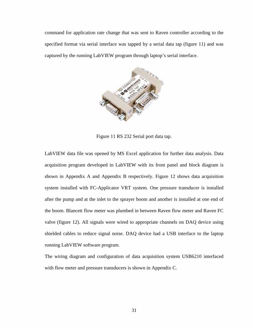
31
command for application rate change that was sent to Raven controller according to the
specified format via serial interface was tapped by a serial data tap (figure 11) and was
captured by the running LabVIEW program through laptop’s serial interface.
Figure 11 RS 232 Serial port data tap.
LabVIEW data file was opened by MS Excel application for further data analysis. Data
acquisition program developed in LabVIEW with its front panel and block diagram is
shown in Appendix A and Appendix B respectively. Figure 12 shows data acquisition
system installed with FC-Applicator VRT system. One pressure transducer is installed
after the pump and at the inlet to the sprayer boom and another is installed at one end of
the boom. Blancett flow meter was plumbed in between Raven flow meter and Raven FC
valve (figure 12). All signals were wired to appropriate channels on DAQ device using
shielded cables to reduce signal noise. DAQ device had a USB interface to the laptop
running LabVIEW software program.
The wiring diagram and configuration of data acquisition system USB6210 interfaced
with flow meter and pressure transducers is shown in Appendix C.

32
Figure 12 USB 6210 Data acquisition system installation with FC-Applicator VRT system.

33
3.6 Rate Controller Inputs
Application rate change commands were triggered via serial interface to the rate
controller from a programmable interface controller (PIC) that was programmed to send
commands in specified format. The chosen PIC was 18F4520 (Microchip Technology
Inc, Chandler, Arizona, USA) that had a RS 232 serial interface. It was programmed in C
language to send different step rate changes to rate controller. Rate changes were chosen
based on expected rate changes observed in as applied data files collected while variably
applying fertilizer using an RT200 VRT system. Two types of rate change commands
were sent to the controller. These changes simulated map and sensor based VRT
applications. The map based simulation consisted of a single rate change command with a
step change of 47 liters per hectare (l/ha) (5 GPA). The rate command alternately stepped
up and down every 20 seconds between 141 and 188 l/ha (15 and 20 GPA). In the
simulated sensor based VRT system the rate change command was sent every second
with rate changes in smaller steps than 47 l/ha (5 GPA) for around 240 seconds. The data
for this were obtained from an as-applied output file from an actual sensor-based VRT
system. The target application rate ranged from 103 l/ha (11 GPA) to 206 l/ha (22 GPA)
with an average of 168 l/ha (18 GPA). The maximum rate change while stepping up was
45 l/ha (4.8 GPA) and while stepping down was 44 l/ha (4.7 GPA). Format for rate
change command sent via serial interface is shown in Appendix D. PIC program for
simulating map based step input is shown in Appendix E and program that simulates
sensor based variable rate input is shown in Appendix F.

34
3.7 Data Collection
Two types of rate change commands were sent to both applicator configurations and data
was collected using LabVIEW program for each applicator configuration and each type
of rate change input. Data were collected for different rate controller parameter settings
as discussed in section 3.2 that determined response time for the two applicator
configurations. For each step test, the sprayer system was made to run at a known
application rate. A rate change command for a desired application was triggered from the
PIC to the rate controller and synchronously data logging from pressure transducers and
flow meter was done using LabVIEW program for 20 s and then another rate change
command was triggered which brought back the application rate to original value and
data was logged for another 20 s. The above procedure was repeated for different
VALVCAL settings on the Raven rate controller that controlled response time and
stability of the controller. The rate change command for step input changed between 141
and 188 l/ha (15 and 20 GPA). In the second type of input, a sensor based VRT system
was simulated where the rate change command was sent every second from PIC with rate
changes in smaller steps than 47 l/ha (5 GPA) for around 240 seconds and data from flow
meter and pressure transducers was logged synchronously using LabVIEW program. This
VRT input test was also repeated for different VALVCAL setting on the Raven rate
controller. For both types of inputs and for both applicator configurations, data
measurements and logging was done with a fixed set of VALCAL parameters. Valve
backlash digit was set to 0 and dead band digit was set to 1 for all measurements. First set
of measurements was made by keeping the valve speed digit at 2 and varying the brake
point digit from 0 to 9. The next set of measurements was made by keeping brake point

35
digit at 2 and varying the valve speed digit from 0 to 9. Every measurement in both
applicator configurations was done for the step input rate change of 47 l/ha (5 GPA) and
also for variable rate inputs that varied every second with smaller step size. Sprayer
ground speed was simulated at 9.7 km/h (6 mph) in the rate controller using its self test
feature for all tests. An optimum controller setting that resulted in a minimum response
time for both applicator configurations and for both types of rate change inputs was found
by analyzing the data log files. Response time was the time between a set point rate
change trigger and when actual flow rate in the boom reached and stabilized to within the
dead band. Measurements were done once for every VALVCAL setting and for each
applicator configuration resulting in one data file for each measurement.
3.8 Overall Response Time Measurement
This section describes a method to measure the overall response time for FC-Applicator
setup. The setup uses a fast close valve with variable orifice nozzles with optimum
controller setting which was determined that resulted in a minimum response time. FC-
Applicator system (figure 12) is extended with a sensor based VRT system. Application
rate changes triggered by PIC are replaced by application rate changes triggered by actual
real-time on the go sensors (figure 13). Sensors used are the green seeker sensors from
actual RT200 VRT system (NTech Industries Inc Ukiah, CA). A roller platform with two
different colored clothing on top of platform is rolled under green seeker sensors of
RT200 system to simulate a trigger for application rate change. The instant (time stamp)
at which green seeker sensors sensed a change in color was a trigger for rate change and
is captured by digital input channel of USB6210 DAQ device with the help of a

36
mechanical push button switch. Data from the green seeker sensor is converted to a
desired rate by an algorithm running on a Recon hand held PC (figure 13). The Recon
sends a rate change command to Raven rate controller via serial interface in the specified
format which was earlier simulated by PIC after it received a change in color indication
from green seeker sensors. This command is synchronously captured by LabVIEW
program along with the time stamp by scanning the serial port. The delay time between
green seeker sensor sensing a color change and time when a rate change command was
sent to rate controller, is measured by calculating the difference in time stamps between
the two events after analyzing the data log file. Overall response time is the sum total of
this delay time and the response time of rate controller measured in previous steps for the
two applicator configurations.

37
Figure 13 Overall response time measurement with FC-Applicator VRT System.

38
CHAPTER IV
RESULTS & DISCUSSION
4.1 Controller Response Time for PWM-Applicator System for Step Input
Table-1 shows controller response time for the PWM-Applicator system consisting of
pulse width modulation (PWM) flow technology with fixed orifice nozzles measured for
different VALVCAL settings. These results are for a step input rate change command.
VALVCAL Digit Response Time, s
Backlash Speed Brake-Point Dead-Band Step-Up Step-Down
0 0 2 1 1.7 1.7 0 1 2 1 1.4 1.5 0 2 2 1 1.7 1.6 0 3 2 1 1.7 1.9 0 4 2 1 2.0 2.3 0 5 2 1 3.1 4.5 0 6 2 1 4.2 6.1 0 7 2 1 6.4 7.4 0 8 2 1 9.0 12.0 0 2 0 1 1.6 1.9 0 2 1 1 1.7 1.8 0 2 2 1 1.7 1.6 0 2 3 1 2.0 9.0 0 2 4 1 13.4 15.7 0 2 5 1 22.0 25.0
Table 1 Controller response time for PWM-Applicator system for step input.

39
Response times for speed digit 9 and for brake point greater than 5 were very high and
are not shown in table 1. The best response time for step input rate change command with
PWM-Applicator was 1.5 s for VALVCAL number 0121 (table 1). For lower numbers of
valve speed and brake point digits, the step-up and step-down time were almost same.
But for higher numbers of valve speed and brake point digits, the step-up and step-down
times were quite different. As seen in table 1, in most cases for higher numbers, the step-
down time was higher compared to step-up time. A sample of data collected using data
acquisition system for response time measurement for step input with VALVCAL 0121 is
shown in figure 14.
Figure 14 Controller response for step input to PWM-Applicator with VALVCAL 0121.

40
The actual application rate displayed a high frequency component with PWM-Applicator
(figure 14). As a result, response time for PWM-Applicator configuration for step input
was measured by a curve fitting technique on measured flow rate in l/ha that used a 5
point moving average function (figure 15). This smoothing function used a moving
average method where each smoothed value was determined by neighboring data points
defined within the span that was 5 points. The smoothing process was weighted because a
regression weight function was defined for the data points contained within the span. The
regression weights for each data point in the span were calculated by the tri-cube function
shown below.
x was the predictor value associated with the response value to be smoothed, xi were the
nearest neighbors of x as defined by the span and d(x) was the distance along the abscissa
from x to the most distant predictor value within the span. The data point to be smoothed
had the largest weight and the most influence on the fit. Data points outside the span had
zero weight and no influence on the fit. A weighted linear least squares regression was
performed. Response time was the time between a set point rate change trigger and when
actual flow rate in the boom reached and stabilized to within 1% of set point value.

41
Figure 15 Controller response time measurement with 5 point moving average on actual
application rate.
4.2 Controller Response Time for PWM-Applicator System for VRT Input
Table 2 shows controller response time for the PWM-Applicator system consisting of
pulse width modulation (PWM) flow technology with fixed orifice nozzles measured for
different VALVCAL settings. These results are for variable rate input with the rate
change command sent every second.
VALVCAL Digit Response Time, s
Backlash Speed Brake-Point Dead-Band
0 0 2 1 0.5 0 1 2 1 0.5 0 2 2 1 0.6

42
0 3 2 1 0.6 0 4 2 1 0.6 0 5 2 1 0.8 0 6 2 1 0.9 0 7 2 1 1.0 0 8 2 1 1.6 0 9 2 1 2.7 0 2 0 1 0.5 0 2 1 1 0.6 0 2 2 1 0.6 0 2 3 1 0.6 0 2 4 1 1.8 0 2 5 1 2.3 0 2 6 1 2.7 0 2 7 1 3.1 0 2 8 1 3.2 0 2 9 1 3.7
Table 2 Controller response time for PWM-Applicator system for variable rate input.
The best response time for PWM-Applicator with variable rate input command was 0.5 s
for VALVCAL number 0121 (table 2) which was also the best VALVCAL number for
step input rate change (table 1). A VALVCAL number of 0201 also resulted in response
time of 0.5 s (table 2). A sample of the data collected using the data acquisition system
for response time measurement with variable rate input for VALVCAL 0121 is shown in
figure 16. In this case, response time was the time between a set point rate change trigger
and when actual flow rate in the boom reached the set point value. The method used to
measure controller response time for variable rate input (figure 16) was different
compared to method used to measure controller response time for step input. As the data
for measured flow rate were collected at 10 Hz, this data of measured flow rate as seen in
figure 16 was shifted back (lagged) by 0.1 s and correlated with set point data. The
number of shifts that resulted in a maximum correlation was considered to be the

43
response time. This time was then calculated in seconds by multiplying the number of
shifts by 0.1 to get controller response time in seconds. This was the response time where
error between the target and actual application rate was at the minimum and the
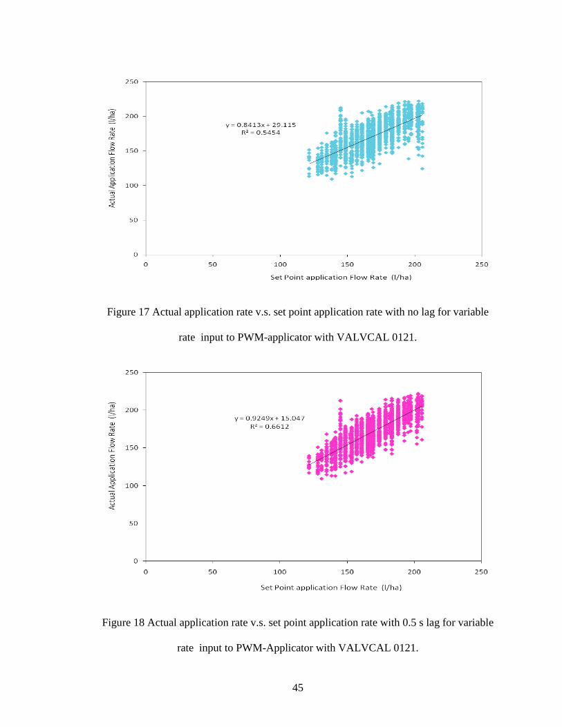
correlation between the target and actual application rate was at the maximum. Figure 17
shows actual application rate graphed as a function of the set point application rate with
no lag for variable rate input sent every second to PWM-Applicator with VALVCAL –
0121. Simply lagging the actual application rate by 0.5 second improved the regression
results (figure 18). Actual application error was calculated by comparing the root mean
square error of actual application rates against set-point application rate for all data points
collected. The actual application error with no lag was 15.5 l/ha (1.7 GPA) whereas the
application error with 0.5 s lag was 13.2 l/ha (1.4 GPA).

44
Figure 16 Controller response for variable rate input sent every second to PWM-Applicator with VALVCAL 0121.
45
Figure 17 Actual application rate v.s. set point application rate with no lag for variable
rate input to PWM-applicator with VALVCAL 0121.
Figure 18 Actual application rate v.s. set point application rate with 0.5 s lag for variable
rate input to PWM-Applicator with VALVCAL 0121.

46
4.3 Controller Response Time for FC-Applicator System for Step Input
Table 3 shows controller response time for the FC-Applicator system consisting of the
Raven fast close (FC) valve with TurboDrop TDVR02 variable orifice nozzles measured
for different VALVCAL settings. These results are for a step input rate change command.
VALVCAL Digit Response Time, s
Backlash Speed Brake-Point Dead-Band
0 0 2 1 OSC* 0 1 2 1 OSC 0 2 2 1 OSC 0 3 2 1 OSC 0 4 2 1 OSC 0 5 2 1 OSC 0 6 2 1 OSC 0 7 2 1 2.1 0 8 2 1 3.6 0 9 2 1 5.1 0 2 0 1 OSC 0 2 1 1 OSC 0 2 2 1 OSC 0 2 3 1 OSC 0 2 4 1 2.5 0 2 5 1 2.8 0 2 6 1 - 0 2 7 1 - 0 2 8 1 - 0 2 9 1 -
Table 3 Controller response time for FC-Applicator system for step input.
* OSC indicates oscillating flow
As seen in table 3, for most of lower valve speed and brake point digits, the Raven FC
valve was unstable and flow to the boom oscillated. These situations are depicted as
‘OSC’ in the ‘Response Time’ column of table 3. Though the flow was unstable with
faster valve speeds (<6), increasing the brake point helped stabilize the system as seen in

47
table 3 for VALVCALs 0241 and 0251. The best response time for FC-Applicator was
2.1 s for VALVCAL number 0721 for step input rate change command (table 3). A
sample of data collected using data acquisition system for response time measurement for
step input with VALVCAL 0721 is shown in figure 19. The high brake point was too
much compensation for fast valve speeds. Controller response time for VALVCAL
numbers with higher brake point digits 0261, 0271, 0281 and 0291 was very high for rate
change command that stepped from high to low and was not considered.
Figure 19 Controller response for step input to FC-Applicator with VALVCAL 0721.
A sample of oscillating flow rate in the boom for step input rate change command for an
aggressive VALVCAL number of 0021 for FC-Applicator is shown in figure 20. The
frequency of oscillation was 1 Hz in all the ‘OSC’ situations.

48
Figure 20 Oscillating controller response for FC-Applicator step input with
VALVCAL 0021.
In case of FC-Applicator configuration too, response time was the time between a set
point rate change trigger and when actual flow rate in the boom reached and stabilized to
within 1% of set point value. Response time was directly measured from the collected
data as there was no noise induced as in case of PWM-Applicator system that used PWM
technology and there was no need to use any curve fitting technique. As compared to the
PWM-Applicator, response time for FC-Applicator while stepping up and while stepping
down was the same.

49
4.4 Controller Response Time for FC-Applicator System for VRT Input
Table 4 shows controller response time for the FC-Applicator system consisting of the
Raven fast close (FC) valve with TurboDrop TDVR02 variable orifice nozzles measured
for different VALVCAL settings. These results are for variable rate input with the rate
change command sent every second.
VALVCAL Digit Response Time, s
Backlash Speed Brake-Point Dead-Band
0 0 2 1 OSC* 0 1 2 1 OSC 0 2 2 1 OSC 0 3 2 1 OSC 0 4 2 1 OSC 0 5 2 1 OSC 0 6 2 1 OSC 0 7 2 1 0.6 0 8 2 1 0.9 0 9 2 1 1.6 0 2 0 1 OSC 0 2 1 1 OSC 0 2 2 1 OSC 0 2 3 1 OSC 0 2 4 1 OSC 0 2 5 1 1.4 0 2 6 1 2.8 0 2 7 1 2.8 0 2 8 1 2.9 0 2 9 1 3.9
Table 4 Controller response time for FC-Applicator system for variable rate input.
* OSC indicates oscillating flow
As seen in table 4, for most of the lower numbers of valve speed digit and brake point
digit, the Raven FC valve was unstable and flow to the boom oscillated. These situations
are depicted as ‘OSC’ in ‘Response Time’ column of table 4. The best response time for

50
FC-Applicator with variable rate input command was 0.6 s for VALVCAL number 0721
(table 4) which was also the best VALVCAL number for step input rate change (table 3).
A sample of the data collected using data acquisition system for response time
measurement with variable rate input for VALVCAL 0721 is shown in figure 21. Even in
this case, the response time was the time between a set point rate change trigger and
when actual flow rate in the boom reached the set point value. The method used to
measure controller response time for variable rate input for FC-Applicator system (figure
21) was similar to the method used to measure controller response time for variable rate
input for PWM-Applicator. As the data for measured flow rate were collected at 10 Hz,
this data of measured flow rate as seen in figure 21 was shifted back (lagged) by 0.1 s and
correlated with set point data. The number of shifts that resulted in a maximum
correlation was considered to be the response time. This time was then calculated in
seconds by multiplying the number of shifts by 0.1 to get controller response time in
seconds.
This was the response time where error between the target and actual application rate was
at the minimum and the correlation between the target and actual application rate was at
the maximum. Figure 22 shows actual application rate graphed as a function of the set
point application rate with no lag for variable rate input sent every second to FC-
Applicator with VALVCAL 0721. Simply lagging the actual application rate by 0.6
second improved the regression results (figure 23). The actual application error with no
lag was 12 l/ha (1.3 GPA) whereas the application error with 0.6 s lag was 8.5 l/ha (0.9
GPA).

51
Figure 21 Controller response for variable rate input sent every second to FC-Applicator with VALVCAL 0721.

52
Figure 22 Actual application rate v.s. set point application rate with no lag for variable
rate input to FC-Applicator with VALVCAL 0721.
Figure 23 Actual application rate v.s. set point application rate with 0.6 s lag for variable
rate input to FC-Applicator with VALVCAL 0721.

53
4.5 Controller Response Time Comparison
The response time for a step input of 47 l/ha (5 GPA) was greater than the response time
for variable rate input where the steps were smaller than 47 l/ha (5 GPA) for both PWM-
Applicator and FC-Applicator. The VALVCAL digits that resulted in a minimum
response time were quite different for both applicator configurations. For PWM-
Applicator configuration, the minimum controller response time occurred at lower valve
speed digits with fixed brake point digit of 2. For FC-Applicator, the minimum response
time of controller was at higher valve speed digits with a fixed brake point digit of 2.
Table 5 shows the VALVCAL number and minimum response times for both types of
inputs for PWM-Applicator that consisted of Capstan pulse width modulation (PWM)
flow technology with fixed orifice nozzles and FC-Applicator that consisted of Raven
fast close (FC) valve with TurboDrop TDVR02 variable orifice nozzles.
Applicator Input VALVCAL
Digit
Response Time,
s
Application Error, l/ha
Backlsh Spd Brake-Pt Dead-Bnd
PWM
Step 0 1 2 1 1.5 12.0
Variable 0 1 2 1 0.5 13.0
FC
Step 0 7 2 1 2.1 7.0
Variable 0 7 2 1 0.6 8.5
Table 5 Minimum controller response time for PWM-Applicator and FC-Applicator
systems with step and variable input and respective VALVCAL digits.

54
Even though we deemed 0.5 s and 0.6 s as the response time to a VRT input for PWM-
Applicator and FC-Applicator systems respectively, (table 5), both systems did not
actually hit the desired rate and there was an application rate error of about 5-8% on an
average in both configurations. The response time for simulated sensor based variable
rate changes was 0.5 s for 0121 VALVCAL number with PWM-Applicator configuration
(table 5). The root mean square application error was 13 l/ha (1.4 GPA). Similarly,
response time for simulated sensor based variable rate change for FC-Applicator
configuration was 0.6 s and the corresponding VALVCAL number being 0721. In this
case, the root mean square application error was 8.5 l/ha (0.9 GPA). It is seen that though
PWM-Applicator consisting of Capstan pulse width modulation (PWM) flow technology
with fixed orifice nozzles had a slightly lower response time than FC-Applicator that
consisted of Raven fast close (FC) valve with TurboDrop TDVR02 variable orifice
nozzles, flow rate and pressure were more stable in FC-Applicator and the root mean
square error was less by 4.5 l/ha (0.5 GPA). The result shows that FC-Applicator
configuration is better suited for sensor based variable rate fertilizer applications where a
rate change is triggered every second with rates changing in smaller steps than 47 l/ha (5
GPA) between 103 l/ha (11 GPA) to 206 l/ha (22 GPA).
From table 5 it is seen that there was a big difference in response time for step input of 47
l/ha (5 GPA) for both applicator configurations. PWM-Applicator performed well with a
response time of 1.5 s as compared to FC-Applicator with response time of 2.1 s. The
root mean square application error for PWM-Applicator was 12 l/ha (1.3 GPA) where as
the root mean square application error for FC-Applicator was 7 l/ha (0.8 GPA). This

55
showed that PWM-Applicator had a smaller response time but larger application error
where as FC-Applicator had a larger response time but smaller application error. This
result of higher RMS application error with lower response time in PWM-Applicator
could be attributed to the fact that PWM-Applicator displayed a high frequency
component in flow rate and pressure in the boom that contributed to higher application
error.
4.6 Boom Pressures in PWM-Applicator System
Pressures at inlet of the boom and at one of the ends of the boom for PWM-Applicator
system were captured by the data acquisition system and analyzed (figure 24), for the
determined optimum VALVCAL number of 0121.
Figure 24 Boom pressures in PWM-Applicator system.

56
Pressures at inlet and end of the boom displayed a high frequency component for PWM-
Applicator system. We believe this high frequency component was due to the alternating
pulses with PWM signal that controlled solenoid valves. However, we were not sampling
fast enough to verify this. There was an average pressure drop of 20 kPa (3 psi) from the
inlet to end of boom.
4.7 Boom Pressures in FC-Applicator System
Pressures at inlet of the boom and at one of the ends of the boom for FC-Applicator
system were also captured by the data acquisition system and analyzed (figure 25), for
the determined optimum VALVCAL number of 0721.
Figure 25 Boom pressures in FC-Applicator system.

57
Pressure at inlet of the boom did display a high frequency component for FC-Applicator
system but did not vary much, as compared to the PWM-Applicator. Pressure at end of
the boom was much stable and did not display a high frequency component. There was an
average pressure drop of 40 kPa (6 psi) from inlet to the end of boom which was double
as compared to PWM-Applicator. We believe this was because of the pressure drop in FC
valve.
58
CHAPTER V
CONCLUSION
Response time of commercially available real-time sensor based VRT equipment with a
Raven SCS 440 rate controller was evaluated with two applicator configurations:
Applicator equipped with Capstan PWM technology with fixed orifice nozzles and an
applicator equipped with Raven FC-Valve with variable orifice nozzles. Pressure, flow
rate, controller input from the sensor system were measured and logged along with time
stamps using a data acquisition system. The logged data were analyzed to determine if
the applied rate correctly followed the desired set-point rates or if there was any delay in
overall response time of VRT equipment for different settings of the rate-controller.
Results also showed that rate controller settings were different for both applicator
configurations for achieving minimum response time of around 0.5 – 0.6 s for variable
rate input. It was seen that though PWM-Applicator consisting of Capstan pulse width
modulation (PWM) flow technology with fixed orifice nozzles had a slightly lower
response time than FC-Applicator that consisted of Raven fast close (FC) valve with
TurboDrop TDVR02 variable orifice nozzles, flow rate and pressure were more stable in
FC-Applicator and the root mean square error was less by 4.5 l/ha (0.5 GPA). Results
implied that controller settings varied with the type of applicator configurations used and
corresponding minimum response time had to be determined for each configuration for
optimum performance of VRT equipment. Results showed that FC-Applicator
configuration was better suited for sensor based variable rate fertilizer applications where
a rate change is triggered every second. There was a big difference in response time for
step input of 47 l/ha (5 GPA) for both applicator configurations, where PWM-Applicator

59
performed well with a response time of 1.5 s as compared to FC-Applicator with
response time of 2.1 s. This showed that PWM-Applicator configuration was better suited
for map based variable rate fertilizer applications where a rate change was triggered less
often in bigger steps. This work would aid in determining minimum spatial resolution
achievable for variable rate application using commercial VRT equipment.

60
CHAPTER VI
FUTURE WORK
This research evaluated the response time of rate controller when used with two different
applicator configurations. These applicator configurations are commonly used in map
based and sensor based VRT equipment, where rate change inputs to controller come
frequently and with different magnitudes. This research did not evaluate the total
response time of real-time sensor based VRT equipment from ‘Sense’ to ‘Spray’. Future
researchers in this area could evaluate the overall response time of this real-time sensor
based VRT equipment. A brief methodology to evaluate this was discussed in section 3.8.
With the results of my research as baseline, future research and tests could be conducted
with different and faster components of the applicator system. The tests could be
conducted by using faster valves, newer technology nozzles and other advanced VRT
equipment and bench mark the response times measured. The rate controller used for my
test was a SCS440 Raven controller. Researchers could also use rate controllers from
different vendors which provide more user control options for controlling the response
time and perform tests to find out combinations of VRT components that result in lower
overall response time. Another area of interest would be to sample the flow and pressure
in the boom at a much higher rate for PWM-Applicator as compared to this research so
that one could better analyze the flow and pressure dynamics in the PWM Applicator
system that used Capstan PWM flow technology.

61
REFERENCES
Anglund, E.A., P.D. Ayers. 2003. Field evaluation of response times for a variable rate (pressure based and injection) liquid chemical applicator. ASAE Paper Number: 001157. St. Joseph, Mich.: ASABE.
Cugati, S.A., W.M. Miller, J.K. Schueller, A.W. Schumann. 2006. Dynamic
characteristics of two commercial hydraulic flow-control valves for a variable-rate granular fertilizer spreader. ASAE Paper Number: 061071, Portland, Oregon
Cugati, S.A., W.M. Miller, J.K. Schueller, A.W. Schumann, S.M. Buchanon, H. K.
Hostler. 2006. Benchmarking the dynamic performance of two commercial variable-rate controllers and components. Transactions of the ASABE. 50(3): 795−802.
Fulton, J.P., S.A. Shearer, S.F. Higgins, M.J. Darr, T.S. Stombaugh. 2005. Rate response
assessment from various granular VRT applicators. Transactions of the ASAE. 48(6): 2095−2103
Godwin, R.J., T.E. Richards, G.A. Wood, J.P. Welsh, S. Knight. 2002. Economic
analysis of precision farming systems. ASAE Paper Number: 02-1019, Chicago, IL.
Raun, W.R., G.V. Johnson. 1999. Improving nitrogen use efficiency for cereal
production. Agronomy journal. 91(3): 357-363. Shearer, S.A., T.S. Stombaugh, J.P. Fulton and T.G. Mueller. 2002. Considerations for
development of variable-rate controller test standard. ASAE Paper Number: 021191, Chicago, IL.
Shoukat Choudhury, M.A.A., N.F. Thornhill, and S.L. Shah. 2005. Modelling valve
stiction. Control Engineering Practice 13(2005):641-658 Solie, J.B., W.R. Raun, R.W. Whitney, M.L. Stone and J.D. Ringer. 1996. Optical sensor
based field element size and sensing strategy for nitrogen application. Transactions of the ASAE. 39: 1983-1992.
Sui, R.J., Alex Thomasson, Jeffrey L. Willers, F. Paul Lee, Rui Wang. 2003. Variable-
rate spray system dynamic evaluation. ASAE Paper Number: 031128, Las Vegas, Nevada.

62
Sumner, H.R., G.C. Rains, P.E. Sumner. 2000. String collectors to determine lag time of injection sprayers. Applied Engineering in Agriculture. 16(5): 471-476.
Yang, C. 2000. A variable rate applicator for controlling rates of two liquid fertilizers.
Applied Engineering in Agriculture. 17(3): 409–417. Zhu, H., R.D. Fox, H.E. Ozkan, R.D. Brazee, R.C. Derksen. 1997. Time delay for
injection sprayers. Transactions of the ASAE. 41(3): 525-530.

63
APPENDICES
Appendix A: Front Panel of LabVIEW Data Acquisition Program

64
Appendix B: Block Diagram of LabVIEW Data Acquisition Program

65
Appendix C: Wiring Diagram of NI USB-6210 Data Acquisition System

66
Appendix D: Raven Controller Rate Change Command Serial Data Format
For changing RATE1 CAL on SCS 440 Raven Controller by remote computer, through
RS-232 serial interface, following needs to be done.
Configuration:
Baud Rate: 1200 or 9600
Parity: NO
Data Bits: 8
Stop Bits: 2
Data stream from Remote Computer to Raven Console:
All request strings have to begin with $R, to indicate a Raven communication string in
the format shown below
$R, RC, <rate_1_cal> <CR> <LF>
For example to change RATE 1 in Raven Controller to 123.4 following string has to be
sent
$R, RC, 1234 <CR> <LF>
Here <CR> and <LF> are carriage return and line feed commands respectively. The unit
for RATE1 is pre-selected by Raven Controller Console.

67
Appendix E: PIC Program for Simulating MAP Based Step Input
#include<18f4520.h>
#device ICD=true
#fuses HS, NOLVP, NOWDT, PUT
#use delay (clock=20000000)
#use rs232 (baud=9600, parity=N,STOP=2,xmit=PIN_C6,rcv=PIN_C7)
void main()
{
int i;
unsigned int16 des_val[256] = { 200 150 }; // Desired Application Rate
WHILE (TRUE)
{
for (i=0;i<2;i++)
{
delay_ms(20000);
printf ("$R,RC,%ld\x0D\x0A",des_val[i]);
}
}
}

68
Appendix F: PIC Program for Simulating Sensor Based Variable Rate Input
#include <18f4520.h>
#device ICD = true
#fuses HS, NOLVP, NOWDT, PUT
#use delay (clock=20000000)
#use rs232 (baud=9600,parity=N,STOP=2,xmit=PIN_C6,rcv=PIN_C7)
void main()
{
int i;
unsigned int16 des_val[256] = { 220 201 216 196 196 196 177 196 181 196
181 177 177 177 181 155 140 144 164 172 172 168 186 196 191 191
172 181 172 181 177 177 159 159 172 177 191 181 168 168 177 181
186 159 148 151 159 181 181 186 191 172 172 155 168 168 172 168
168 177 181 164 151 137 151 172 172 177 172 177 177 177 164 151
148 130 137 140 140 148 151 168 196 201 159 181 217 217 211 211
196 168 177 196 181 177 196 206 206 186 172 177 177 186 186 177
164 144 144 159 151 164 172 168 159 164 181 201 201 211 206 211
201 201 211 217 209 209 196 191 201 191 191 191 186 168 159 164
151 159 164 172 186 196 217 209 155 163 209 217 217 217 217 217
201 201 186 186 196 177 206 220 155 217 211 186 181 186 181 181
186 206 194 179 179 217 206 191 191 168 164 168 181 181 168 164

69
151 168 186 181 191 186 191 196 186 191 181 164 177 177 164 164
151 159 159 168 181 172 168 159 151 177 191 186 168 155 151 137
133 144 159 172 172 159 151 172 186 181 159 164 196 206 196 196
217 209 202 216 220 206 177 220 201 186 164 148 140 137 133 130
130 137 151 159 164 168}; // Desired Application Rate
WHILE (TRUE)
{
for (i=0;i<256;i++)
{
delay_ms (1000);
printf ("$R,RC,%ld\x0D\x0A",des_val[i]);
}
}
}

70
Appendix G: MATLAB Program for frequency analysis using FFT
%%%%%%%%%%%%%%%%%%%%%%%%%%%%%%%%%%%%%%%%%%%%%%%%%%%%%%%%%%%%%%%%%%%%%%% % Flowmeter Signal analysis using FFT to determine frequency component %%%%%%%%%%%%%%%%%%%%%%%%%%%%%%%%%%%%%%%%%%%%%%%%%%%%%%%%%%%%%%%%%%%%%%% Fs = 10; % Sampling frequency T = 1/Fs; % Sample time L = 1414; % Length of signal %%%%%%%%%%%%%%%%%%%%%%%%%%%%%%%%%%%%%%%%%%%%%%%%%%%%%%%%%%%%%%%%%%%%%%%% Actual Flow Rate GPA Aa = xlsread( 'sample' ,4); Aa= Aa(:,1); Aa = Aa((1:L),1); t = (0:L-1)*T; % Time vector figure(1); % Plot the signal in time domain subplot(2,1,1); plot(t(1:L),Aa(1:L)); title( 'Flowmeter Signal' ); xlabel( 'Time (seconds)' ); ylabel( 'Flow Rate (GPA)around Desired Rate' ); NFFT = 2^nextpow2(L); % Next power of 2 from length of y Y = fft(Aa,NFFT)/L; f = Fs/2*linspace(0,1,NFFT/2); % Plot single-sided amplitude spectrum. subplot(2,1,2); plot(f,abs(Y(1:NFFT/2))); title( 'Single-Sided Amplitude Spectrum of Flowmeter Signa l' ); xlabel( 'Frequency (Hz)' ); ylabel( '|Flow|' ); %%%%%%%%%%%%%%%%%%%%%%%%%%%%%%%%%%%%%%%%%%%%%%%%%%%%%%%%%%%%%%%%%%%%%%%% Pressure P1 Aa = xlsread( 'sample' ,5); Aa= Aa(:,1); Aa = Aa((1:L),1); t = (0:L-1)*T; % Time vector figure(2); % Plot the signal in time domain subplot(2,1,1); plot(t(1:L),Aa(1:L));

71
title( 'Pressure Signal P1' ); xlabel( 'Time (seconds)' ); ylabel( 'Pressure P1 psi' ); NFFT = 2^nextpow2(L); % Next power of 2 from length of y Y = fft(Aa,NFFT)/L; f = Fs/2*linspace(0,1,NFFT/2); % Plot single-sided amplitude spectrum. subplot(2,1,2); plot(f,abs(Y(1:NFFT/2))); title( 'Single-Sided Amplitude Spectrum of Pressure P1 Sig nal' ); xlabel( 'Frequency (Hz)' ); ylabel( '|P1|' ); %%%%%%%%%%%%%%%%%%%%%%%%%%%%%%%%%%%%%%%%%%%%%%%%%%%%%%%%%%%%%%%%%%%%%%%% Pressure P2 Aa = xlsread( 'sample' ,6); Aa= Aa(:,1); Aa = Aa((1:L),1); t = (0:L-1)*T; % Time vector figure(3); % Plot the signal in time domain subplot(2,1,1); plot(t(1:L),Aa(1:L)); title( 'Pressure Signal P2' ); xlabel( 'Time (seconds)' ); ylabel( 'Pressure P2 psi' ); NFFT = 2^nextpow2(L); % Next power of 2 from length of y Y = fft(Aa,NFFT)/L; f = Fs/2*linspace(0,1,NFFT/2); % Plot single-sided amplitude spectrum. subplot(2,1,2); plot(f,abs(Y(1:NFFT/2))); title( 'Single-Sided Amplitude Spectrum of Pressure P2 Sig nal' ); xlabel( 'Frequency (Hz)' ); ylabel( '|P2|' );

VITA
Praveen J Bennur
Candidate for the Degree of
Master of Science Thesis: RESPONSE TIME EVALUATION OF REAL-TIME SENSOR BASED
VARIABLE RATE TECHNOLOGY EQUIPMENT Major Field: Bio-Systems & Agricultural Engineering Biographical:
Education: Received a Bachelor of Science degree in Electronics & Communication Engineering from Karnataka University Dharwad, India, Dec 1997; Completed the requirements for the Master of Science in Bio-Systems & Agricultural Engineering at Oklahoma State University, Stillwater, Oklahoma in July, 2009. Professional Memberships: American Society of Agricultural and Biological Engineers Honor Society of Phi Kappa Phi

ADVISER’S APPROVAL: Dr. Randy Taylor
Name: PRAVEEN J BENNUR Date of Degree: July, 2009 Institution: Oklahoma State University Location:Stillwater, Oklahoma Title of Study: RESPONSE TIME EVALUATION OF REAL-TIME SENSOR BASED
VARIABLE RATE TECHNOLOGY EQUIPMENT Pages in Study: 71 Candidate for the Degree of Master of Science
Major Field: Bio-Systems & Agricultural Engineering Scope and Method of Study: The goal of this research was to measure the response time of a commercially available rate controller with two different control valve configurations: pulse width modulated technology with fixed orifice nozzles and a fast-close valve with variable orifice nozzles and to determine the optimum rate-controller parameter setting that results in a minimum response time for both applicator configurations. Parameters pressure, flow rate, controller input from the sensor system were measured and logged using a data acquisition system. The data were analyzed to determine if the applied rate correctly followed the desired set-point rates or if there was any delay in overall response time of rate controller used in commercially available VRT equipment for different settings of the rate-controller. Findings and Conclusions: Results showed that rate controller settings were different for both applicator configurations for achieving minimum response time of around 0.5 – 0.6 s for variable rate input. It was seen that though PWM-Applicator consisting of Capstan pulse width modulation (PWM) flow technology with fixed orifice nozzles had a slightly lower response time than FC-Applicator that consisted of Raven fast close (FC) valve with TurboDrop TDVR02 variable orifice nozzles, flow rate and pressure were more stable in FC-Applicator and the root mean square error was less by 4.5 l/ha (0.5 GPA). Results implied that controller settings varied with the type of applicator configurations used and corresponding minimum response time had to be determined for each configuration for optimum performance of VRT equipment. This work would aid in determining minimum spatial resolution achievable for variable rate application using commercial VRT equipment.

Abstract:
Real-time sensor based variable rate technology (VRT) equipment is complex
with many different components working together to achieve a desired output. The
equipment provides rate- controller set-point every second creating more challenges in
terms of functioning of each component and its response time to achieve a variable rate
application with existing rate-controllers, valves and nozzles. All components involved
operate on inputs from the other thereby inducing a time delay. This time delay among
components questions the credibility on performance of sensor based commercially
available VRT equipment and its overall response time. Response time of commercially
available real-time sensor based VRT system was evaluated with two applicator
configurations: Applicator equipped with Capstan PWM technology with fixed orifice
nozzles and an applicator equipped with Raven FC-Valve with variable orifice nozzles.
Parameters pressure, flow rate, controller input from the sensor system were measured
and logged using a data acquisition system. The data were analyzed to determine if the
applied rate correctly follows the desired set-point rates or if there is any delay in overall
response time of VRT equipment for different settings of the rate-controller. Results
showed that rate-controller settings were different for both applicator configurations for
achieving minimum response time of around 0.5 s. This work will aid in determining the
spatial resolution for variable rate application using commercially VRT equipment.