SUBSPACE-BASED COOPERATIVE SPECTRUM ...digital.library.okstate.edu/etd/Rao_okstate_0664M_10867.pdfSUBSPACE-BASED COOPERATIVE SPECTRUM SENSING FOR COGNITIVE RADIOS By RAGHAVENDRA UDUPI

SUBSPACE-BASED COOPERATIVE SPECTRUM SENSING FOR

COGNITIVE RADIOS

By

RAGHAVENDRA UDUPI RAO

Bachelor of Engineering in Telecommunication

Vishveshwaraya Technological University

Bangalore, Karnataka, India

2006

Submitted to the Faculty of theGraduate College of

Oklahoma State Universityin partial fulfillment ofthe requirements for

the Degree ofMASTER OF SCIENCE

May, 2010

SUBSPACE-BASED COOPERATIVE SPECTRUM SENSING FOR

COGNITIVE RADIOS

Thesis Approved:

Dr. Qi Cheng

Thesis Advisor

Dr. Martin T Hagan

Dr. Nazanin Rahnavard

Dr. A Gordon Emslie

Dean of the Graduate College

ii

ACKNOWLEDGMENTS

I would firstly like to thank my advisor Dr. Qi Cheng. Without her constant guidance

and support, this work would have never lifted off the ground and reach this stage. I

would also like to thank her for giving me the opportunity to work with her as a Re-

search assistant and in course, introducing me to the wonderful world of Statistical Signal

Processing and Cognitive radios.

I would like to thank my parents: Radhakrishna Rao and Tara Rao for their never

ending support and encouragement. Without their backing I could have not come this

far.

I would like to extend my sincere gratitude towards the members of the Statistical

signal processing lab for all the help that they have given.

Last but not the least, I would like to thank all my roommates and friends here in

Stillwater, for always being there and providing me with an excellent social life.

iii

TABLE OF CONTENTS

Chapter Page

1 INTRODUCTION 1

1.1 Spectrum scarcity and Cognitive Radio . . . . . . . . . . . . . . . . . . . . 1

1.2 Motivation . . . . . . . . . . . . . . . . . . . . . . . . . . . . . . . . . . . . 5

1.3 Organization of Thesis . . . . . . . . . . . . . . . . . . . . . . . . . . . . . 8

2 Literature review 9

2.1 Conventional Spectrum Sensing Techniques . . . . . . . . . . . . . . . . . . 10

2.1.1 Matched Filter . . . . . . . . . . . . . . . . . . . . . . . . . . . . . 10

2.1.2 Energy Detector . . . . . . . . . . . . . . . . . . . . . . . . . . . . 11

2.1.3 Cyclostationary Feature Detection . . . . . . . . . . . . . . . . . . . 12

2.2 Narrow Band Spectrum Sensing Techniques . . . . . . . . . . . . . . . . . 12

2.3 Wide Band Spectrum Sensing Techniques . . . . . . . . . . . . . . . . . . . 14

2.4 Collaborative Spectrum Sensing . . . . . . . . . . . . . . . . . . . . . . . . 15

3 Subspace-based Cooperative spectrum sensing 22

3.1 Problem Formulation . . . . . . . . . . . . . . . . . . . . . . . . . . . . . . 22

3.2 Subspace-based spectrum sensing algorithm . . . . . . . . . . . . . . . . . 23

3.2.1 Estimation of K . . . . . . . . . . . . . . . . . . . . . . . . . . . . 26

3.3 Cooperative spectrum sensing algorithm . . . . . . . . . . . . . . . . . . . 28

3.3.1 Data Association . . . . . . . . . . . . . . . . . . . . . . . . . . . . 28

3.3.2 Fusion of Estimates, the linear unbiased estimate . . . . . . . . . . 33

4 Simulations 36

4.1 Fading only . . . . . . . . . . . . . . . . . . . . . . . . . . . . . . . . . . . 36

4.2 Shadowing plus fading . . . . . . . . . . . . . . . . . . . . . . . . . . . . . 39

iv

5 CONCLUSIONS 47

A Derivation of the elements of the Q matrix 48

B Analysis of ESPRIT 52

C Tracy-Widom distribution 53

D More on k-means clustering technique using the MDL principle 55

D.1 k-means . . . . . . . . . . . . . . . . . . . . . . . . . . . . . . . . . . . . . 55

D.2 MDL principle . . . . . . . . . . . . . . . . . . . . . . . . . . . . . . . . . . 57

D.3 Instantiations of the MDL-Algorithm . . . . . . . . . . . . . . . . . . . . . 57

BIBLIOGRAPHY 61

v

LIST OF TABLES

Table Page

4.1 Detection performance of the proposed method for all the three configura-

tions. σ2 = 10dB, K=3, ρ = 10dB. . . . . . . . . . . . . . . . . . . . . . . 41

vi

LIST OF FIGURES

Figure Page

1.1 Spectrum utilization. . . . . . . . . . . . . . . . . . . . . . . . . . . . . . . 1

1.2 Cognitive Radio cycle. . . . . . . . . . . . . . . . . . . . . . . . . . . . . . 3

1.3 Spectrum hole concept. . . . . . . . . . . . . . . . . . . . . . . . . . . . . . 5

2.1 Implementation of an energy detector. . . . . . . . . . . . . . . . . . . . . 11

2.2 Implementation of a cyclostationary feature detector. . . . . . . . . . . . . 12

2.3 An advantage of cooperative spectrum sensing in cognitive radio (CR) net-

works is depicted here; CR 1 is shadowed over the sensing channel and CR

3 is shadowed over the reporting channel, but the presence of PU is not

missed because of CR 2 reporting to the base station. . . . . . . . . . . . 16

2.4 Hidden terminal problem. . . . . . . . . . . . . . . . . . . . . . . . . . . . 17

2.5 Exposed terminal problem. . . . . . . . . . . . . . . . . . . . . . . . . . . . 18

2.6 Collaborative sensing with a fusion center. . . . . . . . . . . . . . . . . . . 20

2.7 Collaborative sensing without a fusion center. . . . . . . . . . . . . . . . . 21

3.1 PSD of a wide BOI. . . . . . . . . . . . . . . . . . . . . . . . . . . . . . . . 23

3.2 Illustration of the data association algorithm. SNR=-15dB, D = 10. There

are only three PU signals in the source located at 0.31, 1.57 and 2.83

rad/sample, respectively. . . . . . . . . . . . . . . . . . . . . . . . . . . . . 29

4.1 The percentage of correct detections as a function of σ2 using one, five and

ten SUs, respectively. K = 3. . . . . . . . . . . . . . . . . . . . . . . . . . 37

4.2 MSE performance as a function of 1/σ2 of all three PU signals using one,

five and ten SUs, respectively.MSE performance of all three fusion tech-

niques. Number of SUs collaborating is fixed at 10. . . . . . . . . . . . . . 38

vii

4.3 The percentage of correct detections as a function of 1/σ2 for various con-

figurations. K = 3. . . . . . . . . . . . . . . . . . . . . . . . . . . . . . . . 39

4.4 MSE performance for different configurations. . . . . . . . . . . . . . . . . 40

4.5 Probability of correct detection ofK as a function of the shadowing variance

ρ. . . . . . . . . . . . . . . . . . . . . . . . . . . . . . . . . . . . . . . . . . 42

4.6 Optional caption for list of figures . . . . . . . . . . . . . . . . . . . . . . . 43


4.8 The probability of correct detection as a function of the number of SUs.

ρ =10dB. . . . . . . . . . . . . . . . . . . . . . . . . . . . . . . . . . . . . 45

4.9 MSE of estimation of ω1 as a function of the number of SUs. ρ =10dB. . . 45


C.1 Tracy-Widom density plots, corresponding to the values of β = 1, 2 . . . . 54

D.1 Illustration of the performance of the k-means algorithm, when initialized

with eight centers (a) and four centers (b). . . . . . . . . . . . . . . . . . . 56

D.2 Iterative algorithm. . . . . . . . . . . . . . . . . . . . . . . . . . . . . . . . 58

viii

CHAPTER 1

INTRODUCTION

1.1 Spectrum scarcity and Cognitive Radio

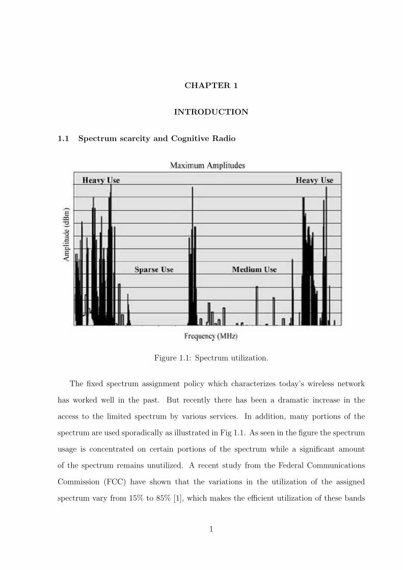
Figure 1.1: Spectrum utilization.

The fixed spectrum assignment policy which characterizes today’s wireless network

has worked well in the past. But recently there has been a dramatic increase in the

access to the limited spectrum by various services. In addition, many portions of the

spectrum are used sporadically as illustrated in Fig 1.1. As seen in the figure the spectrum

usage is concentrated on certain portions of the spectrum while a significant amount

of the spectrum remains unutilized. A recent study from the Federal Communications

Commission (FCC) have shown that the variations in the utilization of the assigned

spectrum vary from 15% to 85% [1], which makes the efficient utilization of these bands

1

a more significant problem than the scarcity of the spectrum [2].

Spectrum utilization can be improved if the users are more aware of the radio environ-

ment around them. Cognitive Radio (CR), with its ability to sense its radio environment

and exploit the information to opportunistically find unused frequency bands which is

best suited for the user’s communication requirements, is viewed as a novel approach to

improve spectrum utilization. [3] has provided the following definition of a cognitive radio.

”Cognitive radio is an intelligent wireless communication system that is aware of its

surrounding environment (i.e., outside world), and uses the methodology of understanding-

by-building to learn from the environment and adapt its internal states to statistical vari-

ations in the incoming RF stimuli by making corresponding changes in certain operating

parameters (e.g., transmit-power, carrier-frequency, and modulation strategy) in real-time,

with two primary objectives in mind:

• highly reliable communications whenever and wherever needed;

• efficient utilization of the radio spectrum.”

The major tasks of a cognitive radio can then be classified as [3]:

• Radio scene analysis: In this task we deal with detecting the unused frequency

band. The other task is to determine the interference temperature, which provides

a measure of the acceptable amount of interference at a particular frequency band at

the receiver side, so any transmission in the band is considered to be sat- isfactory if

the noise is below the interference limit and is considered to be harmful if the noise

is above the interference temperature limit.

• Channel state estimation: The focus is on determining the channel capacity for

which the state of the channel also needs to be determined.

• Spectrum management: The main goal of this task is efficient spectrum sharing of

the vacant channels detected in the radio scene analysis stage. This can be achieved

by an appropriate channel allocation scheme, power allocation scheme and proper

selection of modulation strategies, etc.

2

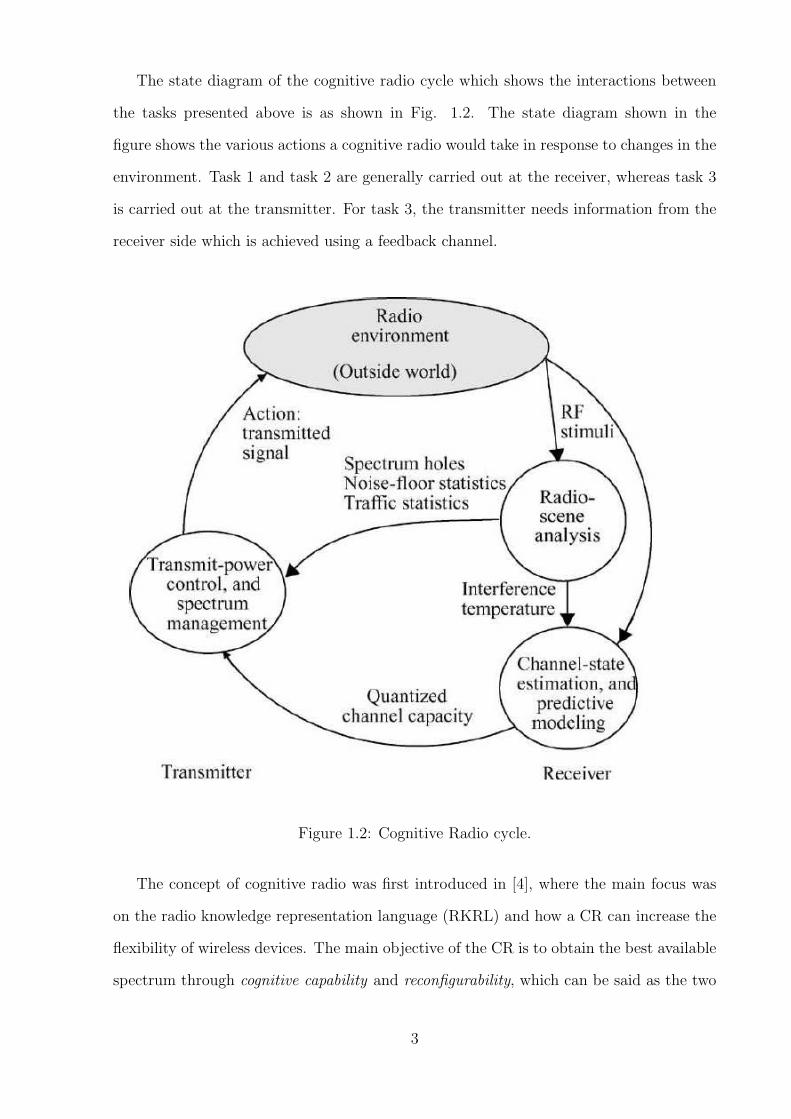
The state diagram of the cognitive radio cycle which shows the interactions between

the tasks presented above is as shown in Fig. 1.2. The state diagram shown in the

figure shows the various actions a cognitive radio would take in response to changes in the

environment. Task 1 and task 2 are generally carried out at the receiver, whereas task 3

is carried out at the transmitter. For task 3, the transmitter needs information from the

receiver side which is achieved using a feedback channel.

Figure 1.2: Cognitive Radio cycle.

The concept of cognitive radio was first introduced in [4], where the main focus was

on the radio knowledge representation language (RKRL) and how a CR can increase the

flexibility of wireless devices. The main objective of the CR is to obtain the best available

spectrum through cognitive capability and reconfigurability, which can be said as the two

3

main characteristics of the CR.

• Cognitive capability : Cognitive capability is the ability of the radio to sense the

information from its radio environment. This cannot simply be realized by moni-

toring the power levels in some frequency band of interest but more sophisticated

techniques are required in order to capture variations in the radio environment and

avoid interference to the licensed users. Through this capability, the unused portions

of the spectrum at a specific time or location can be identified. The best spectrum

and other operating parameters can be then selected.

• Reconfigurability : Reconfigurability enables the radio to be dynamically programmed

according to the radio environment. The CR can be programmed to transmit and

receive on a variety of frequencies and also change its parameter like power level,

modulation technique etc.

From the above two characteristics we see that once the CR senses the radio environ-

ment and chooses the best available channel, it should be able to change all its protocols

in order to suite the conditions in the available spectrum. Hence a lot of new functional-

ities are required to be added to the existing protocols in order to achieve the cognitive

ability.

The major tasks of a CR cycle can be summarized as follows:

• Spectrum sensing: CRs do not have any licensed frequency band to work with.

Through spectrum sensing they identify unused frequency bands for their operation.

This process has to be fast enough to go through a large chunk of the spectrum

quickly and accurate enough to not miss any unused band while maintaining the

false alarm rates.

• Spectrum management: Once the unused bands are recognized, the CR must choose

the best available spectrum for its communication needs.

• Spectrum mobility: When a communication has been established between CRs there

can be cases wherein the licensed user comes back again. The CRs must be able to

4

maintain seamless communication during the transition to another spectrum. This

function is analogous to the hand off function in cellular networks.

• Spectrum sharing: When many CRs coexist in the same area, a fair spectrum

scheduling method should be provided amongst them.

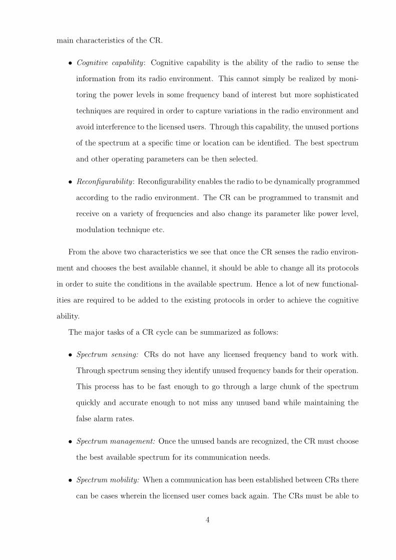
The ultimate objective of a CR is to obtain the best available spectrum. Since most of

the spectrum is already assigned, the most important challenge is to share the spectrum

without interfering with the transmission of licensed users. Through spectrum sensing,

the CR is able to find temporally unused spectrum, which is referred to as spectrum hole

or white space. If the licensed user comes back then the CR has to use other spectrum

holes or alter its transmission power to avoid interference. The spectrum hole concept is

further illustrated with the help of Fig 1.2.

Figure 1.3: Spectrum hole concept.

1.2 Motivation

From the above functionalities we can say that the spectrum sensing is the most important

part of the CR cycle. There are several approaches for sensing which are proposed includ-

5

ing matched filter detection, energy detection and the cyclocstationary feature detection

. The energy detector being a non coherent detection method is the most widely used

method since it proves to be more robust against multipath fading than the methods men-

tioned above. However, the energy detector is vulnerable to noise uncertainty and needs

to have an accurate knowledge of the noise floor. Another disadvantage of the above men-

tioned detection schemes is that they are narrowband, i.e., they concentrate one channel

at a time. Wideband sensing methods makes the spectrum sensing more efficient as they

sense the whole bandwidth in one go. For wideband sensing we use signal estimation and

detection methods using the eigendecomposition of statistical covariance matrices. These

methods can be broadly classified as subspace methods and the eigenvalue decomposition

separates the so-called structured (carrier signal) and the unstructured (noise) compo-

nents. The successful decomposition of the eigen values and eigen vectors provides a lot

of information about the properties of a spectrum band. The problem of estimating the

sinusoidal frequencies from uniformly sampled measurements has received considerable

attention in signal processing. There are many established methods such as MUSIC and

ESPRIT(also known as SURE) where the properties of the sinusoidal frequency estimates

are fairly understood.

Although the above mentioned methods provide an accurate estimate of the frequen-

cies, the estimation done at a particular CR always has a higher chance of error than when

done centrally. This happens due to the multipath and shadowing effects of the wireless

channel. Shadowing can cause the secondary user to completely miss the detection of a

particular primary user. Co-operation between several CRs can help combat shadowing

and fading effects. This method is very robust against severe shadowing environments as

the probability of all users in deep fade is very low. On the other hand due to the high

frequency values used for communication (typical operation occurs in the GHz range) the

effects of multipath fading vary significantly with minute displacements of the secondary

user (consider a band at 3 GHz, the wavelength at this range is 10 cm. So a displacement

of 2.5 cm will cause a phase shift of 90 degrees). To combat multipath effects the use of

multiple antennas at the secondary user is also suggested.

6

The main advantage of Co-operative schemes is that they provide better immunity to

fading and shadowing effects even when the channel is poorly modeled. Spatial diversity

has been explored extensively in wireless communication to combat fading. It can be

similarly applied in the context of spectrum sensing and such cooperation among several

secondary users provides significant advantages in alleviating the effect of destructive

channel fading. While most of the existing cooperative spectrum sensing schemes are

built on narrowband sensing approaches such as energy detection, there has not been

much focus on cooperative schemes for wideband sensing. Wideband sensing techniques

such as wavelet and subspace methods pose the problem of estimating the locations of

PU signals in the frequency domain. When cooperation is involved, we face the challenge

of grouping the estimates from different CRs that correspond to the same PU signal, i.e.,

the data association problem. Another important issue that should be addressed while

combining estimates is whether the fusion method is insensitive to a few bad estimates.

Bad estimates are defined as the estimates which are generated from false alarms and are

assumed to have significant errors. These issues motivate the use of the robust technique

for the fusion procedure.

In this paper, a cooperative wideband sensing scheme based on the subspace method

is explored. Specifically, the eigen-decomposition of the sample covariance matrix is con-

ducted at individual secondary users equipped with multiple antennas. The estimation

results regarding the number of primary signals and their corresponding carrier frequen-

cies within the band of interest (BOI) are combined at a fusion center. We address the

problem of data association through robust clustering techniques using the k-means al-

gorithm and the minimum description length (MDL) principle, which help not only in

grouping the estimates but also in rejecting bad estimates as outliers. In order to obtain

the optimal form of the linear fusion rule, the variances of the local frequency estimates

are derived using the bootstrap method, which is shown to improve the accuracy of final

estimates compared to using the existing result of the asymptotic variance for a large

number of samples. The effects of fading can be effectively suppressed through the collab-

oration among secondary users using the proposed method, leading to improved detection

7

performance and more accurate carrier frequency estimation.

1.3 Organization of Thesis

The remainder of the thesis is organized as follows. A literature review is presented

in chapter 2 wherein we have an overview of the various methods used for spectrum

sensing including some of the latest ongoing work. The problem under consideration is

formulated in section 3.1. In Section 3.2, the subspace method for spectrum sensing at

each SU using multiple antennas is derived. The cooperative scheme by combining local

estimates is proposed in Section 3.3. Chapter 4 demonstrates the effectiveness of the

proposed algorithm through simulations. Conclusions and future work are provided in

the last chapter.

8

CHAPTER 2

Literature review

Being the focus of this thesis, spectrum sensing by far is the most important component

in the cognitive radio cycle. Spectrum sensing is the task of getting to know the spectrum

usage and the existence of licensed PUs in a particular geographical area. This can be

achieved by using geolocation and database, beacons, or by local spectrum sensing at

SUs. There are many challenges which the spectrum sensing cycle poses to a CR. Some

of them can be listed as:

• Hardware Requirements : Spectrum sensing requires a CR to sense vast parts of the

spectrum in a short duration of time. This means that a CR should be equipped

with a sophisticated RF front end, have high resolution ADCs and must have a lot

of signal processing blocks.

• Hidden Terminal Problem: The hidden terminal problem is a very common occur-

rence in wireless networks. For a CR this is poses a bigger problem since it cannot

afford to miss out the presence of a particular PU. Cooperation is often used as a

solution to this problem and is discussed in detail in the next section.

• Spread Spectrum Users : For commercial wireless applications there are two kinds

of users: fixed spectrum and spread spectrum users. Spread spectrum users are

particularly hard to detect since they occupy large parts of the spectrum at low

powers. This problem can be avoided to an extent if perfect synchronization is

achieved and the hopping sequence is known. however, it is not straightforward to

design algorithms to detetct such users.

• Security : A malicious CR can emulate a PU signal to hog the entire bandwidth in

a particular area. This will render all the CRs in that area useless. Therefore, the

9

spectrum sensing should be able to differentiate between a signal and the actual PU

signal. Various methods have been proposed to counter the issue like checking the

coordinates of the sensed signal and identifying unique signatures of the PU signals.

• Sensing Frequency and Duration: A CR cannot spend all its time in sensing. The

performance of the most of the sensing algorithms greatly increase with the increase

in the number of samples take. A bound must be kept on this metric so that the

duration is minimized for the required performance levels. The frequency of sensing

is another issue that a CR must think about. If a PU signal is known to use the

spectrum frequently then the CR must increase the frequency of sensing and vice

versa.

The main focus is on the local spectrum due to its lower infrastructure requirements

and broader applications. Although spectrum sensing has been generally known as mea-

suring the radio frequency energy over the spectrum; when cognitive radio is considered,

it becomes a more general term involving knowing the spectrum usage characteristics,

determining the number of signals and their modulation techniques, bandwidth, carrier

frequency etc.. This chapter will first focus on the conventional spectrum sensing tech-

niques and then move on to explain some of the latest literature on spectrum sensing.

2.1 Conventional Spectrum Sensing Techniques

2.1.1 Matched Filter

Since a matched filter maximizes the signal to noise ratio, it is the optimal method for

any kind of signal detection [5]. However, matched-filtering requires the cognitive radio

to demodulate the received signals and therefore needs prior information about the sig-

nal, e.g., the packet length, the modulation type, pulse shaping. Although these can be

worked around by storing them in the cognitive radio memory, the main problem of the

matched filter is that it has to attain coherency for demodulation by performing synchro-

nization and channel equalization. For certain class of primary users this is still possible

as they provide synchronization details through pilots, preambles and spreading codes.

10

The advantage of a matched filter is that it requires the lowest amount of computational

complexity to achieve the required performance levels. However, as explained before, the

drawback is that cognitive radio will be required to store a lot of information about pri-

mary users and it also needs to change the receiver characteristics for different types of

primary users [6].

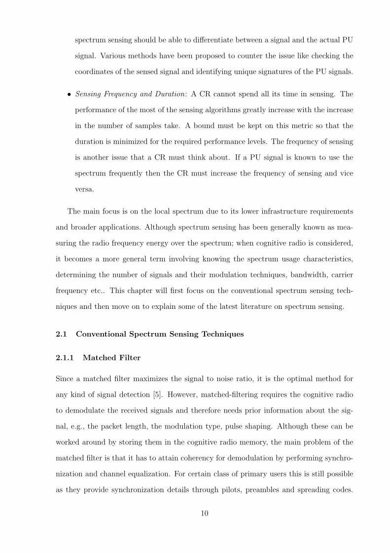
2.1.2 Energy Detector

Energy detector is a suboptimal detector that performs noncoherent detection. The work-

ing of a energy detector is similar to that of a spectrum analyzer where the received signal

is first sampled, then converted to the frequency domain by taking the fast fourier trans-

form (FFT) followed by squaring the coefficients and then taking the average. This value

is then compared to a predetermined threshold to check for the presence of a PU [8].

The whole process is outlined in Fig 2.1 [7]. Processing gain of an energy detector is

directly proportional to the number of bins used and observation time. However, the

computational time time is much more than that of the matched filter which is expected

due to the non-coherent feature [9]. Due to its simplicity and the non requirement of prior

knowledge, the energy detector becomes a very popular choice for spectrum sensing. But

there are several drawbacks that restricts its usage. First, the performance of a energy

detector is strongly related to the choice of the threshold, which makes the method highly

susceptible to unknown or changing noise levels. Second, energy detectors cannot differ-

entiate between a PU, noise and other SUs. Lastly, an energy detector does not work for

advanced modulation schemes like spread spectrum and frequency hopping techniques.

Figure 2.1: Implementation of an energy detector.

11

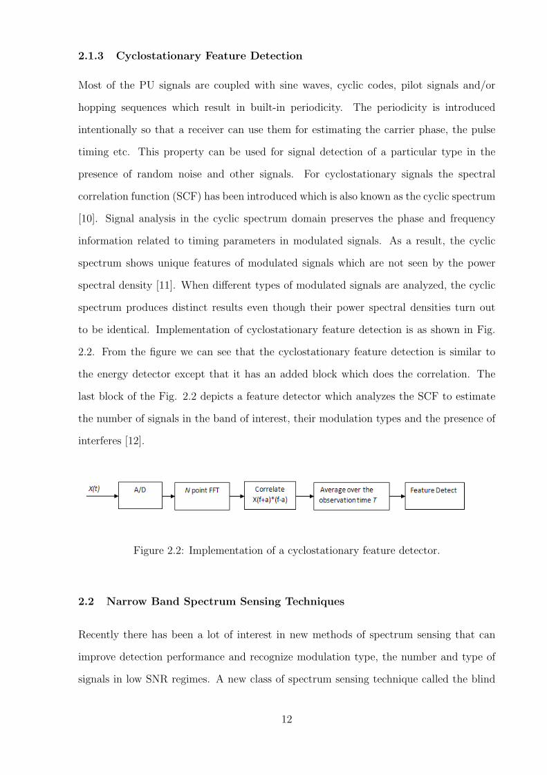
2.1.3 Cyclostationary Feature Detection

Most of the PU signals are coupled with sine waves, cyclic codes, pilot signals and/or

hopping sequences which result in built-in periodicity. The periodicity is introduced

intentionally so that a receiver can use them for estimating the carrier phase, the pulse

timing etc. This property can be used for signal detection of a particular type in the

presence of random noise and other signals. For cyclostationary signals the spectral

correlation function (SCF) has been introduced which is also known as the cyclic spectrum

[10]. Signal analysis in the cyclic spectrum domain preserves the phase and frequency

information related to timing parameters in modulated signals. As a result, the cyclic

spectrum shows unique features of modulated signals which are not seen by the power

spectral density [11]. When different types of modulated signals are analyzed, the cyclic

spectrum produces distinct results even though their power spectral densities turn out

to be identical. Implementation of cyclostationary feature detection is as shown in Fig.

2.2. From the figure we can see that the cyclostationary feature detection is similar to

the energy detector except that it has an added block which does the correlation. The

last block of the Fig. 2.2 depicts a feature detector which analyzes the SCF to estimate

the number of signals in the band of interest, their modulation types and the presence of

interferes [12].

Figure 2.2: Implementation of a cyclostationary feature detector.

2.2 Narrow Band Spectrum Sensing Techniques

Recently there has been a lot of interest in new methods of spectrum sensing that can

improve detection performance and recognize modulation type, the number and type of

signals in low SNR regimes. A new class of spectrum sensing technique called the blind

12

spectrum sensing method is introduced in [13] - [16]. As discussed in section 2.1, for con-

ventional spectrum sensing techniques, some kind of information about the primary user

or the accurate knowledge of the noise floor is needed. In blind spectrum sensing tech-

niques, there is no need for any kind of information that has to be predetermined. [13] uses

Akaike weights as a decision metric for the presence of a PU signal. The Akaike weights

can be interpreted as an estimate of the probability that the received signal distribution

fits the Gaussian one. Since pure noise can be modeled by a Gaussian distribution, an

empty band can be detected by analyzing the Akaike weights information. In [14], the

authors use the properties of eigenvalues of the signal covariance matrix for detection

purposes. The ratio of the maximum and minimum eigenvalues of the covariance matrix

is proposed as a statistic for signal detection. In [15] a modified energy detector is intro-

duced wherein, instead of directly comparing the received signal energy with a threshold

(which is the predetermined noise floor), the ratio of the signal energy and the minimum

eigenvalue of the signal covariance matrix is compared to a threshold. The difference here

is that this new threshold can be derived from the input samples by using the random

matrix theory and does not depend on the knowledge of the noise floor. Further analysis

is conducted in [16] and through new results in random matrix theory, the true distribu-

tion of the maximum and minimum eigenvalues of the signal covariance matrix is derived.

This makes the detector more accurate and its results tractable. Apart from using the

eigenvalues of the covariance matrix [17] directly uses the elements of the covariance ma-

trix for its detection purposes. Since noise is uncorrelated, its covariance matrix diagonal,

therefore the ratio of the diagonal elements to the non diagonal elements tends to be

larger if a PU is present. The threshold chosen for this detector can also be derived using

random matrix theory and is independent of the noise variance.

Although the covariance matrix based detection and maximum-minimum eigenvalue

detection are not related to noise uncertainty, their performances tend to degrade signif-

icantly at low SNR. [18] talks about improving the low SNR performance by using the

non-Gaussian property of a PU signal. The proposed algorithm calculates the statisti-

cal difference between the Gaussian noise and the primary user signal by applying the

13

Bussgang theorem. The Bussgang theorem states that when a real Gaussian stationary

process passes through a memoryless nonlinear device, the crosscorrelation function of

the input and the output is proportional to the autocorrelation function of the input [19].

Using this theorem [18] provides a statistical test to differentiate between a PU signal

and pure Gaussian noise. Going on the same lines of detecting a change of the statistical

properties of the received signal, [20] proposes a new spectrum sensing technique which

uses the quickest detection theory. Statistical tests are carried out to detect the change of

the observation distribution as quickly as possible. This helps us attain quick and robust

spectrum sensing. The well known cumulative sum (CUSUM) algorithm is modified to

include the generalized likelihood ratio test to form a new algorithm called successive

refinement.

The use of neural networks for signal classification is proposed in [21], where the

authors use the cyclostationary feature detector and combine it with a neural network set

to form a system which not only performs signal detection but also signal classification.

2.3 Wide Band Spectrum Sensing Techniques

Till now all the spectrum sensing methods that have been described have one thing in

common, they concentrate on one channel at a time. Having a sensing algorithm which

can scan a wide band of interest (BOI) at once is very advantageous since it reduces the

sensing time and also helps spectrum management algorithms get the information about

all the free bands at once.

Multicarrier communications generally use filter banks at the receiver side to effectively

demodulate the signals. [3] and [22]propose to use these filter banks to double up as

a spectrum analyzer. Thus signal analysis comes at no additional cost as the output

of the filter banks gives you the power spectral density of all the carrier frequencies

used for communication. Another approach is to use a tunable narrowband band pass

filter at the RF front end of the CR, over which the usual narrowband spectrum sensing

techniques can be performed. Recently, the same idea is adopted in [23] for OFDM

communication systems. Multiple sub bands are assumed to be present in which only

14

some of the orthogonal channels are being used by PUs. To detect the number of free

channels, the signal is received and demodulated into subbands by the discrete fourier

transform process and the subchannels are then checked for the presence of a PU by jointly

optimizing a bank of multiple narrowband detectors (energy detector)in order to improve

the opportunistic throughput capacity of cognitive radios. In general, a PU may use larger

bandwidth than just a subband, that is, a subset of adjacent subbands simultaneously.

In such a scenario, the spectrum monitoring can be considerably enhanced provided that

the SU has some knowledge about the group of subbands which may be occupied by a

specific PU [24]. By grouping, it means the integration of the information obtained from

such a group of subbands. All subbands in a group will have a common status regarding

the presence or the absence of the PU. Therefore, only one binary hypothesis is required

for a given group which results in a faster and more accurate spectrum sensing.

Wavelets have been used for wideband sensing [25] [26]. Given the power spectral

density (PSD) of the spectrum, a wavelet transform can be used to detect the edges

where transition from an occupied band to an empty band or vice versa occurs. By

looking at the power levels between these edges, the frequency spectrum can be classified

as empty or not.

2.4 Collaborative Spectrum Sensing

As mentioned in section 1.2, sensing done at a single SU is not always reliable, irrespective

of the accuracy shown by the method used. Fig. 2.3 shows a simple scenario where the

advantage of collaborative sensing is observed. The most common problem faced by

an SU is depicted in Fig. 2.4. As we can see, cognitive radio (CR) C is out of the

transmission range of PU A, and can miss out the presence of the PU. This will cause

interference when it tries to communicate with CR B. This is commonly known as the

hidden terminal problem. Another issue faced by a CR terminal, which is also generally

present in wireless networks is the exposed terminal problem. In Fig. 2.5, CR C can be

termed as the exposed terminal. CR C cannot communicate with CR D because it is

“exposed” to the transmission of PU B. The problem here is that CR C does not know

15

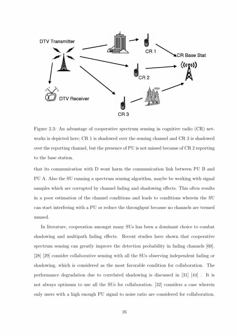
Figure 2.3: An advantage of cooperative spectrum sensing in cognitive radio (CR) net-

works is depicted here; CR 1 is shadowed over the sensing channel and CR 3 is shadowed

over the reporting channel, but the presence of PU is not missed because of CR 2 reporting

to the base station.

that its communication with D wont harm the communication link between PU B and

PU A. Also the SU running a spectrum sensing algorithm, maybe be working with signal

samples which are corrupted by channel fading and shadowing effects. This often results

in a poor estimation of the channel conditions and leads to conditions wherein the SU

can start interfering with a PU or reduce the throughput because no channels are termed

unused.

In literature, cooperation amongst many SUs has been a dominant choice to combat

shadowing and multipath fading effects. Recent studies have shown that cooperative

spectrum sensing can greatly improve the detection probability in fading channels [60].

[28] [29] consider collaborative sensing with all the SUs observing independent fading or

shadowing, which is considered as the most favorable condition for collaboration. The

performance degradation due to correlated shadowing is discussed in [31] [44] . It is

not always optimum to use all the SUs for collaboration. [32] considers a case wherein

only users with a high enough PU signal to noise ratio are considered for collaboration.

16

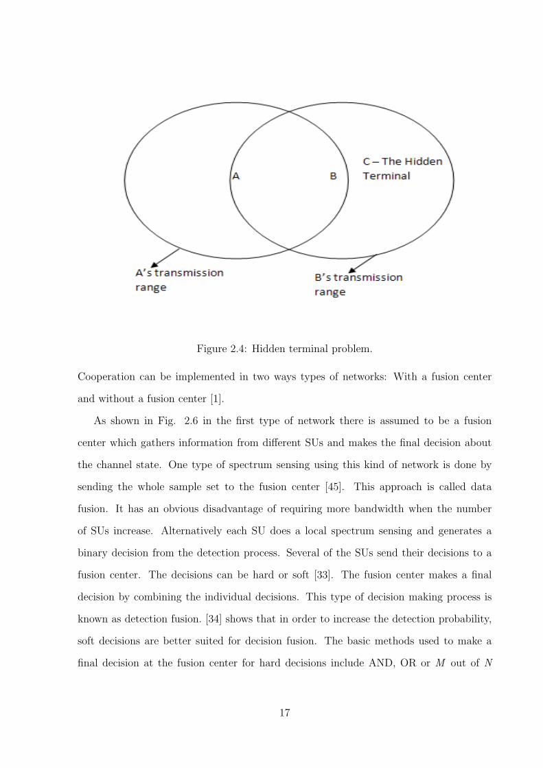
Figure 2.4: Hidden terminal problem.

Cooperation can be implemented in two ways types of networks: With a fusion center

and without a fusion center [1].

As shown in Fig. 2.6 in the first type of network there is assumed to be a fusion

center which gathers information from different SUs and makes the final decision about

the channel state. One type of spectrum sensing using this kind of network is done by

sending the whole sample set to the fusion center [45]. This approach is called data

fusion. It has an obvious disadvantage of requiring more bandwidth when the number

of SUs increase. Alternatively each SU does a local spectrum sensing and generates a

binary decision from the detection process. Several of the SUs send their decisions to a

fusion center. The decisions can be hard or soft [33]. The fusion center makes a final

decision by combining the individual decisions. This type of decision making process is

known as detection fusion. [34] shows that in order to increase the detection probability,

soft decisions are better suited for decision fusion. The basic methods used to make a

final decision at the fusion center for hard decisions include AND, OR or M out of N

17

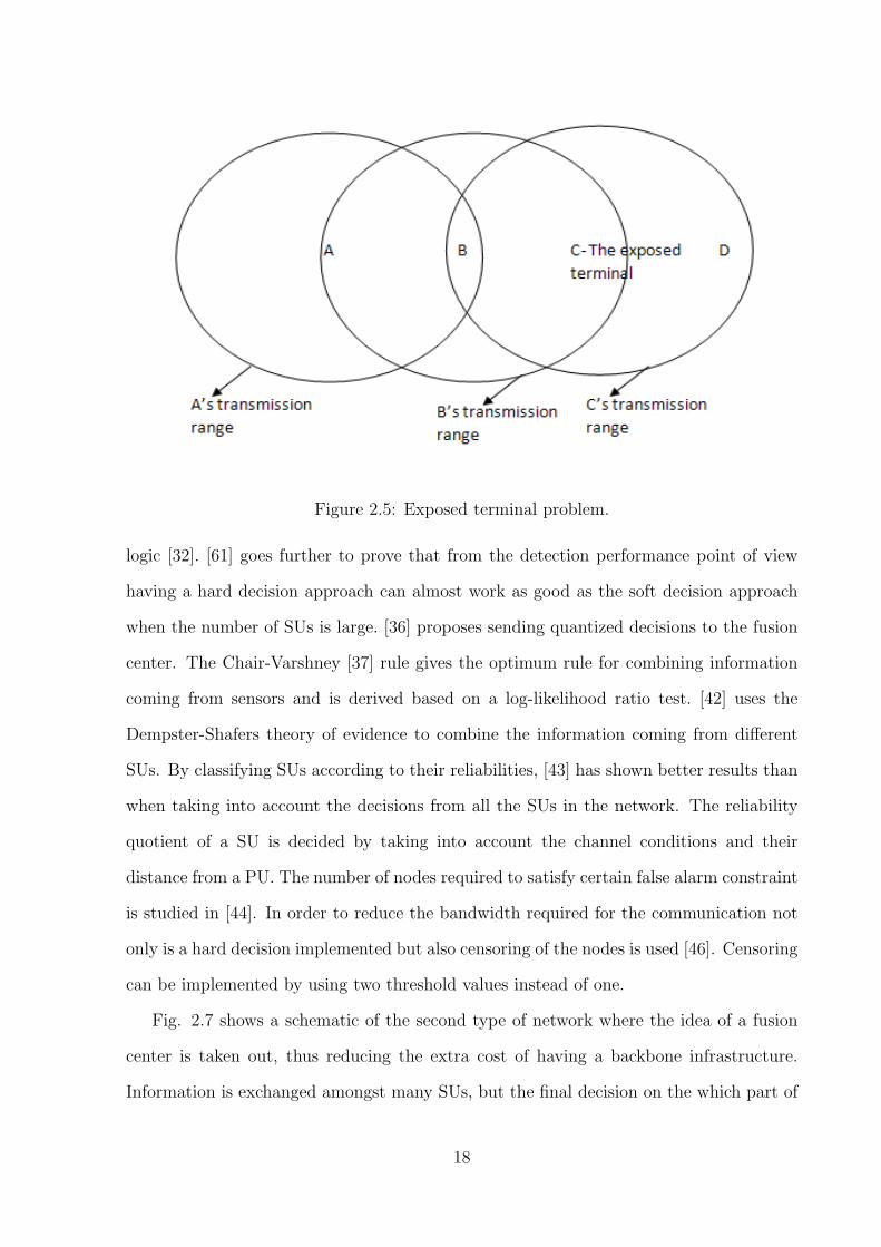
Figure 2.5: Exposed terminal problem.

logic [32]. [61] goes further to prove that from the detection performance point of view

having a hard decision approach can almost work as good as the soft decision approach

when the number of SUs is large. [36] proposes sending quantized decisions to the fusion

center. The Chair-Varshney [37] rule gives the optimum rule for combining information

coming from sensors and is derived based on a log-likelihood ratio test. [42] uses the

Dempster-Shafers theory of evidence to combine the information coming from different

SUs. By classifying SUs according to their reliabilities, [43] has shown better results than

when taking into account the decisions from all the SUs in the network. The reliability

quotient of a SU is decided by taking into account the channel conditions and their

distance from a PU. The number of nodes required to satisfy certain false alarm constraint

is studied in [44]. In order to reduce the bandwidth required for the communication not

only is a hard decision implemented but also censoring of the nodes is used [46]. Censoring

can be implemented by using two threshold values instead of one.

Fig. 2.7 shows a schematic of the second type of network where the idea of a fusion

center is taken out, thus reducing the extra cost of having a backbone infrastructure.

Information is exchanged amongst many SUs, but the final decision on the which part of

18

spectrum to use is taken locally. This type of spectrum sensing architecture for cogni-

tive radio is studied in [47] [48] [49]. Observations at different SUs are shared amongst

neighbors to improve the sensing abilities of the whole network. In order to reduce the

bandwidth used for communication, [50] proposed the exchange of only the final decision

of the sensing process. Clustering of SUs without the help of a central unit is discussed

in [51]. A SU with a high PU SNR or closer to the PU will collaborate and form a cluster

with other SUs who are far away. This will help all the SUs in the cluster make a correct

decision. An incremental gossiping approach termed as GUESS (gossiping updates for

efficient spectrum sensing) is proposed in [52]. The algorithm helps in the coordination

between the SUs with advantages like low complexity and minimum protocol overhead. To

increase the efficiency in coordination, incremental aggregation and randomized gossiping

algorithms are also studied in [52].

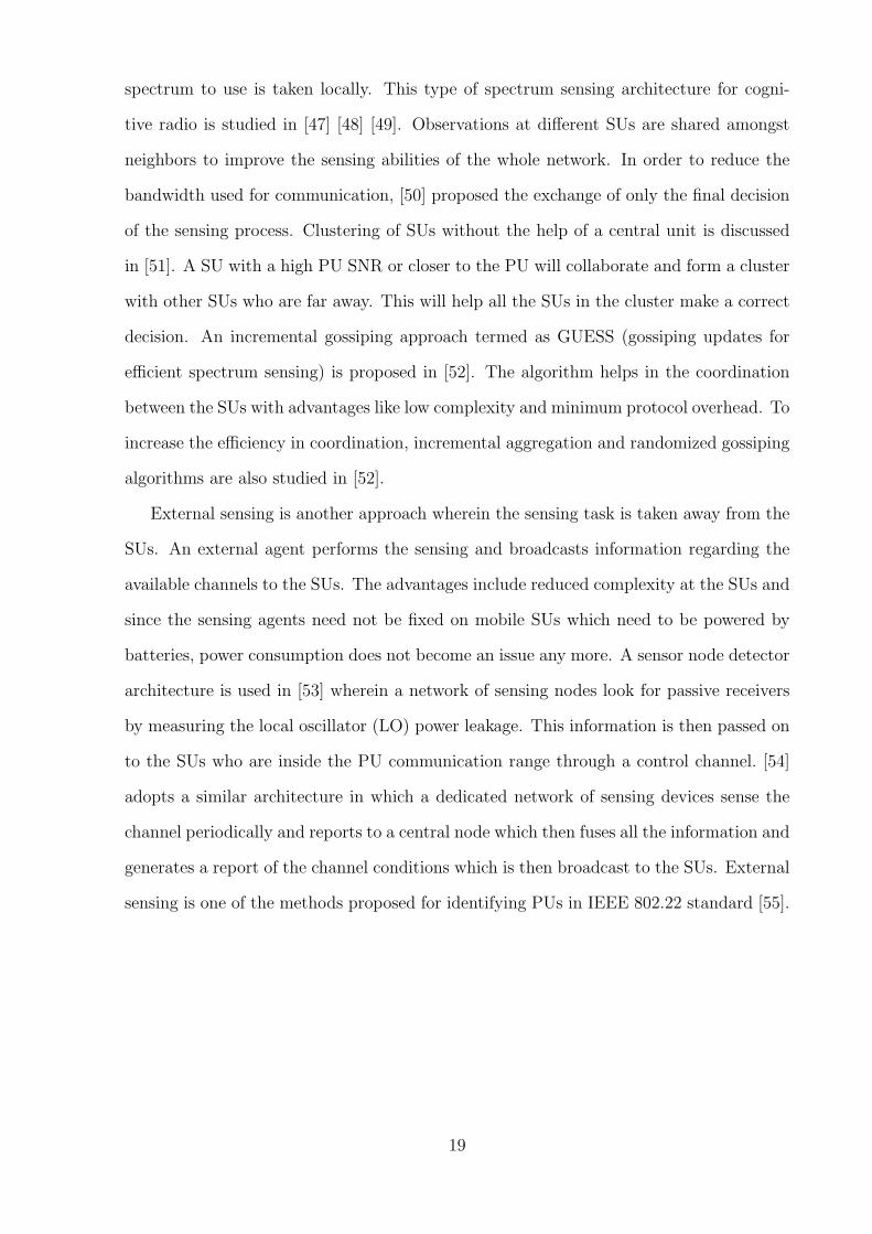
External sensing is another approach wherein the sensing task is taken away from the

SUs. An external agent performs the sensing and broadcasts information regarding the

available channels to the SUs. The advantages include reduced complexity at the SUs and

since the sensing agents need not be fixed on mobile SUs which need to be powered by

batteries, power consumption does not become an issue any more. A sensor node detector

architecture is used in [53] wherein a network of sensing nodes look for passive receivers

by measuring the local oscillator (LO) power leakage. This information is then passed on

to the SUs who are inside the PU communication range through a control channel. [54]

adopts a similar architecture in which a dedicated network of sensing devices sense the

channel periodically and reports to a central node which then fuses all the information and

generates a report of the channel conditions which is then broadcast to the SUs. External

sensing is one of the methods proposed for identifying PUs in IEEE 802.22 standard [55].

19

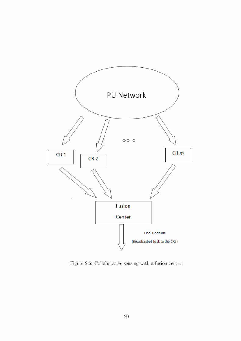
Figure 2.6: Collaborative sensing with a fusion center.

20

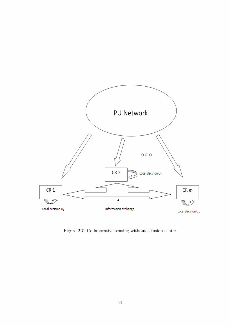
Figure 2.7: Collaborative sensing without a fusion center.

21

CHAPTER 3

Subspace-based Cooperative spectrum sensing

3.1 Problem Formulation

Assume that there are Q secondary users trying to access the spectrum opportunistically,

with each user having Dq antennas, q = 1, 2, . . . , Q. There are K PU signals in the

bandwidth of interest, each with a carrier frequency fk, k = 1, 2, . . . , K. ωk is defined as

ωk = 2πfk∆T rad/sample, where ∆T is the sampling interval. The sampled signal sensed

at the dth antenna of the qth secondary user, d = 1, 2, . . . , Dq, can be expressed using the

following model,

zqd(n) =K∑

k=1

hqdkSk(n)ejωkn + wqd(n) n = 1, 2, · · · , N (3.1)

Here, hqdk is the complex channel gain for the kth PU signal at the dth antenna of the

qth secondary user. It is assumed to be zero mean1 and statistically independent across

antennas, SUs and PU signals. Sk(n) is the sample complex envelope of the kth PU signal

and is assumed to be a wide-sense stationary random process. wqd(n)Nn=1 is a sequence

of white Gaussian noise with mean zero, variance σ2 and is assumed to be statistically

independent across secondary users and their antennas. For most communication systems,

transmitted signals generally experience slow fading [63]. Therefore, we assume that the

channel gains do not change for the N samples. wqd(n)Nn=1 is a sequence of white

Gaussian noise with mean zero, variance σ2 and is assumed to be statistically independent

across secondary users and their antennas.

Fig. 3.1 shows the PSD of a wide BOI of interest. As we can see that there are

many kinds of signals each centered at different carrier frequencies and occupying dif-

1It is assumed to be a homogeneous scattering environment without line of sight.

22

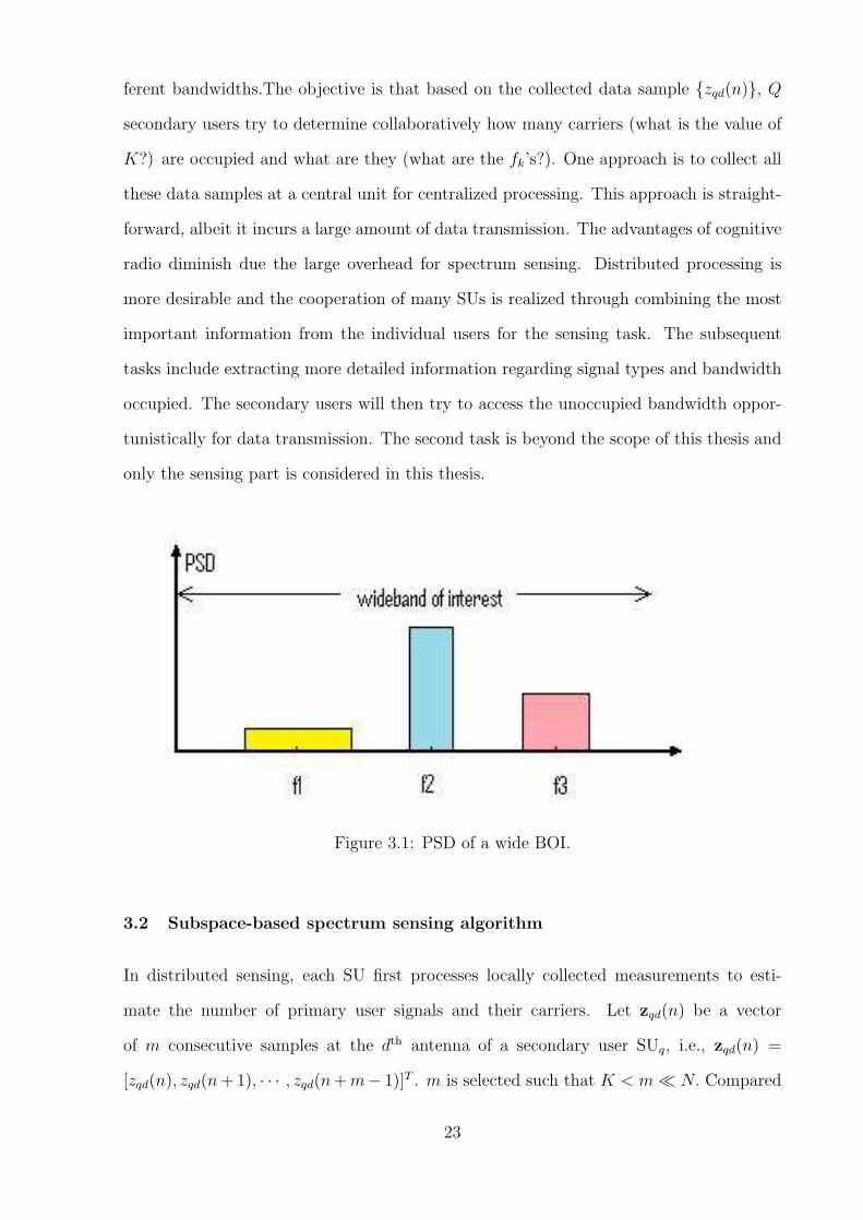
ferent bandwidths.The objective is that based on the collected data sample zqd(n), Q

secondary users try to determine collaboratively how many carriers (what is the value of

K?) are occupied and what are they (what are the fk’s?). One approach is to collect all

these data samples at a central unit for centralized processing. This approach is straight-

forward, albeit it incurs a large amount of data transmission. The advantages of cognitive

radio diminish due the large overhead for spectrum sensing. Distributed processing is

more desirable and the cooperation of many SUs is realized through combining the most

important information from the individual users for the sensing task. The subsequent

tasks include extracting more detailed information regarding signal types and bandwidth

occupied. The secondary users will then try to access the unoccupied bandwidth oppor-

tunistically for data transmission. The second task is beyond the scope of this thesis and

only the sensing part is considered in this thesis.

Figure 3.1: PSD of a wide BOI.

3.2 Subspace-based spectrum sensing algorithm

In distributed sensing, each SU first processes locally collected measurements to esti-

mate the number of primary user signals and their carriers. Let zqd(n) be a vector

of m consecutive samples at the dth antenna of a secondary user SUq, i.e., zqd(n) =

[zqd(n), zqd(n+1), · · · , zqd(n+m− 1)]T . m is selected such that K < m ≪ N. Compared

23

with the sampling rate 1/∆T , signal Sk(n) can be considered as a slow-varying process.

We can assume that within m consecutive samples, Sk(n) ≈ Sk(n+ i), i = 1, . . . ,m− 1,

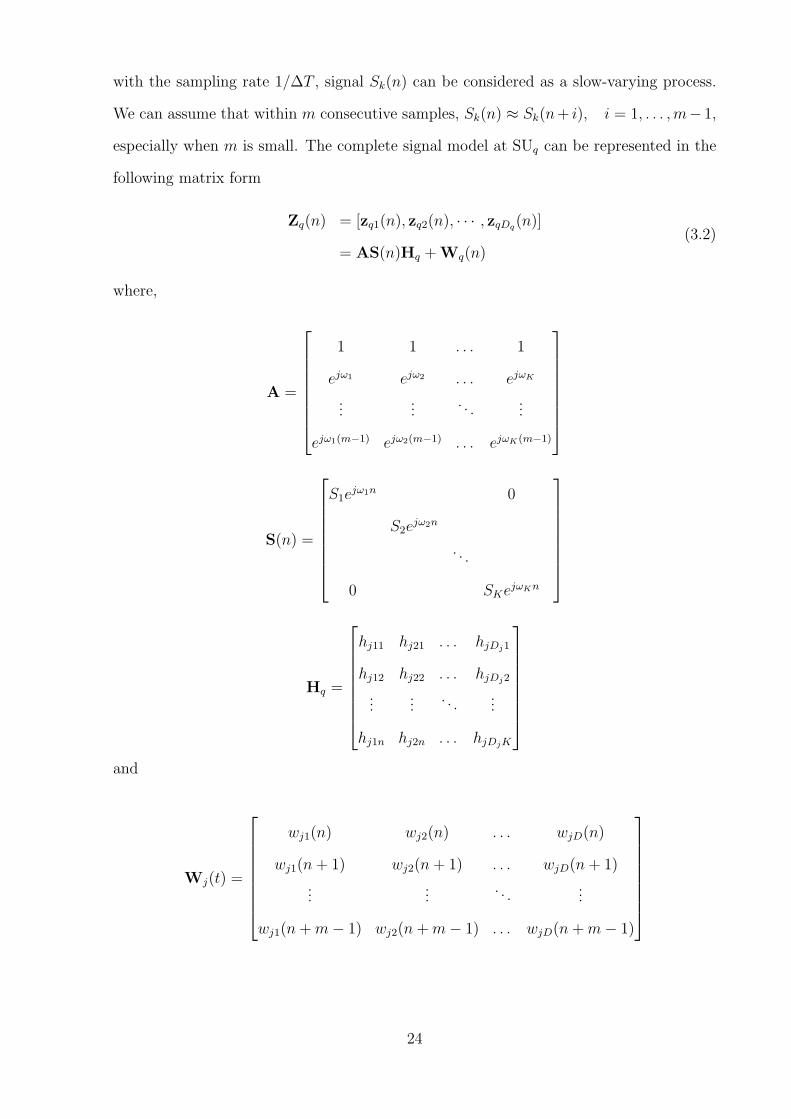
especially when m is small. The complete signal model at SUq can be represented in the

following matrix form

Zq(n) = [zq1(n), zq2(n), · · · , zqDq(n)]

= AS(n)Hq +Wq(n)(3.2)

where,

A =

1 1 . . . 1

ejω1 ejω2 . . . ejωK

......

. . ....

ejω1(m−1) ejω2(m−1) . . . ejωK(m−1)

S(n) =

S1ejω1n 0

S2ejω2n

. . .

0 SKejωKn

Hq =

hj11 hj21 . . . hjDj1

hj12 hj22 . . . hjDj2

......

. . ....

hj1n hj2n . . . hjDjK

and

Wj(t) =

wj1(n) wj2(n) . . . wjD(n)

wj1(n+ 1) wj2(n+ 1) . . . wjD(n+ 1)

......

. . ....

wj1(n+m− 1) wj2(n+m− 1) . . . wjD(n+m− 1)

24

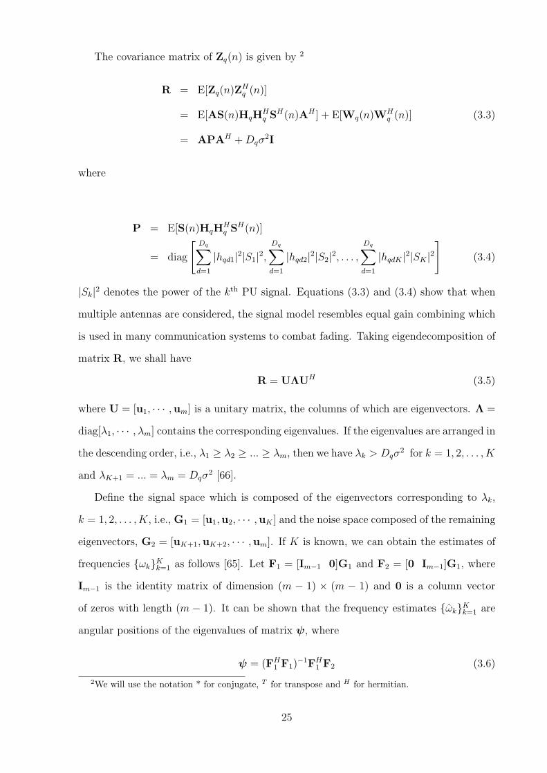
The covariance matrix of Zq(n) is given by 2

R = E[Zq(n)ZHq (n)]

= E[AS(n)HqHHq S

H(n)AH ] + E[Wq(n)WHq (n)] (3.3)

= APAH +Dqσ2I

where

P = E[S(n)HqHHq S

H(n)]

= diag

[Dq∑

d=1

|hqd1|2|S1|

2,

Dq∑

d=1

|hqd2|2|S2|

2, . . . ,

Dq∑

d=1

|hqdK |2|SK |

2

](3.4)

|Sk|2 denotes the power of the kth PU signal. Equations (3.3) and (3.4) show that when

multiple antennas are considered, the signal model resembles equal gain combining which

is used in many communication systems to combat fading. Taking eigendecomposition of

matrix R, we shall have

R = UΛUH (3.5)

where U = [u1, · · · ,um] is a unitary matrix, the columns of which are eigenvectors. Λ =

diag[λ1, · · · , λm] contains the corresponding eigenvalues. If the eigenvalues are arranged in

the descending order, i.e., λ1 ≥ λ2 ≥ ... ≥ λm, then we have λk > Dqσ2 for k = 1, 2, . . . , K

and λK+1 = ... = λm = Dqσ2 [66].

Define the signal space which is composed of the eigenvectors corresponding to λk,

k = 1, 2, . . . , K, i.e., G1 = [u1,u2, · · · ,uK ] and the noise space composed of the remaining

eigenvectors, G2 = [uK+1,uK+2, · · · ,um]. If K is known, we can obtain the estimates of

frequencies ωkKk=1 as follows [65]. Let F1 = [Im−1 0]G1 and F2 = [0 Im−1]G1, where

Im−1 is the identity matrix of dimension (m − 1) × (m − 1) and 0 is a column vector

of zeros with length (m − 1). It can be shown that the frequency estimates ωkKk=1 are

angular positions of the eigenvalues of matrix ψ, where

ψ = (FH1 F1)

−1FH1 F2 (3.6)

2We will use the notation * for conjugate, T for transpose and H for hermitian.

25

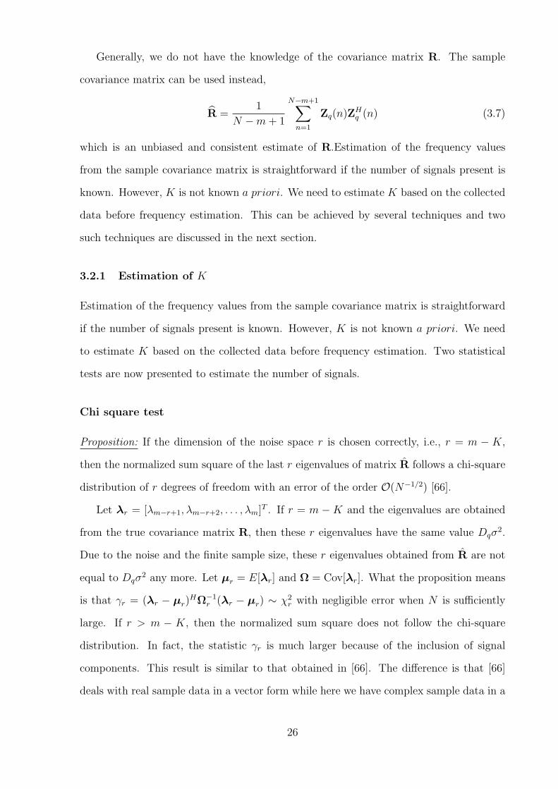
Generally, we do not have the knowledge of the covariance matrix R. The sample

covariance matrix can be used instead,

R =1

N −m+ 1

N−m+1∑

n=1

Zq(n)ZHq (n) (3.7)

which is an unbiased and consistent estimate of R.Estimation of the frequency values

from the sample covariance matrix is straightforward if the number of signals present is

known. However, K is not known a priori. We need to estimate K based on the collected

data before frequency estimation. This can be achieved by several techniques and two

such techniques are discussed in the next section.

3.2.1 Estimation of K

Estimation of the frequency values from the sample covariance matrix is straightforward

if the number of signals present is known. However, K is not known a priori. We need

to estimate K based on the collected data before frequency estimation. Two statistical

tests are now presented to estimate the number of signals.

Chi square test

Proposition: If the dimension of the noise space r is chosen correctly, i.e., r = m − K,

then the normalized sum square of the last r eigenvalues of matrix R follows a chi-square

distribution of r degrees of freedom with an error of the order O(N−1/2) [66].

Let λr = [λm−r+1, λm−r+2, . . . , λm]T . If r = m −K and the eigenvalues are obtained

from the true covariance matrix R, then these r eigenvalues have the same value Dqσ2.

Due to the noise and the finite sample size, these r eigenvalues obtained from R are not

equal to Dqσ2 any more. Let µr = E[λr] and Ω = Cov[λr]. What the proposition means

is that γr = (λr − µr)HΩ−1

r (λr − µr) ∼ χ2r with negligible error when N is sufficiently

large. If r > m − K, then the normalized sum square does not follow the chi-square

distribution. In fact, the statistic γr is much larger because of the inclusion of signal

components. This result is similar to that obtained in [66]. The difference is that [66]

deals with real sample data in a vector form while here we have complex sample data in a

26

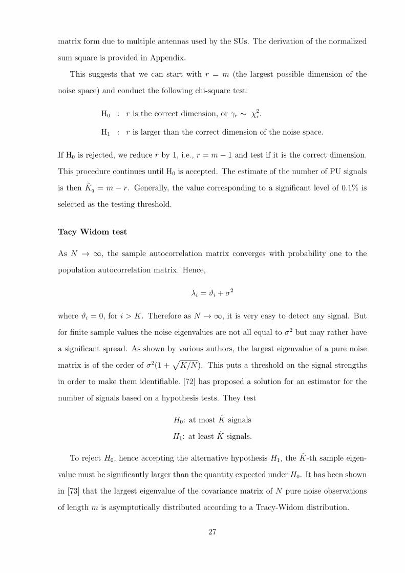
matrix form due to multiple antennas used by the SUs. The derivation of the normalized

sum square is provided in Appendix.

This suggests that we can start with r = m (the largest possible dimension of the

noise space) and conduct the following chi-square test:

H0 : r is the correct dimension, or γr ∼ χ2r.

H1 : r is larger than the correct dimension of the noise space.

If H0 is rejected, we reduce r by 1, i.e., r = m− 1 and test if it is the correct dimension.

This procedure continues until H0 is accepted. The estimate of the number of PU signals

is then Kq = m − r. Generally, the value corresponding to a significant level of 0.1% is

selected as the testing threshold.

Tacy Widom test

As N → ∞, the sample autocorrelation matrix converges with probability one to the

population autocorrelation matrix. Hence,

λi = ϑi + σ2

where ϑi = 0, for i > K. Therefore as N → ∞, it is very easy to detect any signal. But

for finite sample values the noise eigenvalues are not all equal to σ2 but may rather have

a significant spread. As shown by various authors, the largest eigenvalue of a pure noise

matrix is of the order of σ2(1 +√K/N). This puts a threshold on the signal strengths

in order to make them identifiable. [72] has proposed a solution for an estimator for the

number of signals based on a hypothesis tests. They test

H0: at most K signals

H1: at least K signals.

To reject H0, hence accepting the alternative hypothesis H1, the K-th sample eigen-

value must be significantly larger than the quantity expected under H0. It has been shown

in [73] that the largest eigenvalue of the covariance matrix of N pure noise observations

of length m is asymptotically distributed according to a Tracy-Widom distribution.

27

limm,N→∞

Pλ1 < αm,N + sγm,N = Fβ(s)

where β=1,2 for real and complex values respectively and the expressions for αm,N

and γm,N are given in [72]. Using this property of the largest eigen value corresponding

to the noise matrix, the estimator for the number of signals can be derived as

argK maxλK > σ2(K)[αm−K,N + s(τ)γm−K,N ]

τ is the required rate of false alarm and s(τ) can be obtained by inversing the Tracy-

Widom distribution. σ2(K) is the estimator for the noise level. An important point for

this test is the accurate estimation for the noise level which is discussed in detail in [72].

More on the tracy widom distribution is provided in the Appendix.

3.3 Cooperative spectrum sensing algorithm

The subspace-based PU signal detection and their carrier frequency estimation at indi-

vidual secondary users are not robust due to shadowing effects. There might be cases

where none of the antennas on a secondary user receive signals of respectable strengths.

To combat the effects of shadowing, a cooperative scheme with a fusion center among

the secondary users is considered. Each of the SUs implements a local subspace-based

algorithm and send its estimates (ωkKq

k=1) to the fusion center. The communication cost

is much reduced compared to sending all of the collected samples to the fusion center. To

effectively fuse the estimates, the fusion center has to deal with two problems,

1. There is a necessity of data association, i.e., to decide which estimates from different

secondary users belong to the same PU signal.

2. Once associated, how to fuse the estimates from different secondary users.

3.3.1 Data Association

Assume that SUd has Kd frequency estimates ωkdKj

k=1, j = 1, . . . , Q, 0 ≤ Kj < m. The

idea behind our data association algorithm is to group those estimates that are close

28

to each other into clusters. Each cluster can have at most one frequency estimate from

each SU. The estimate after fusion of the estimates within each cluster will be the final

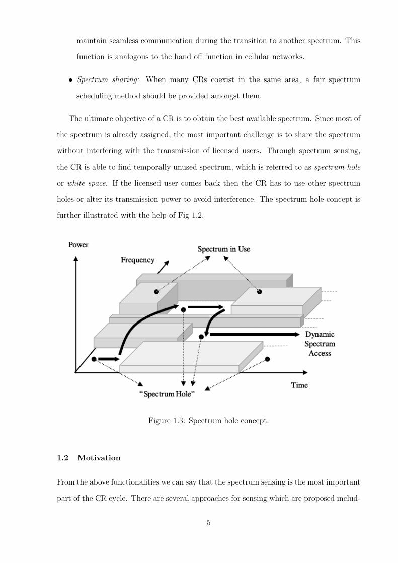
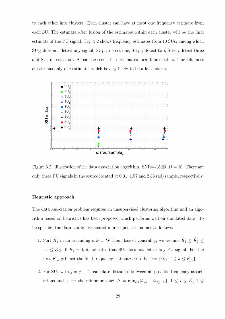
estimate of the PU signal. Fig. 3.2 shows frequency estimates from 10 SUs, among which

SU10 does not detect any signal, SU1−3 detect one, SU4−6 detect two, SU7−8 detect three

and SU9 detects four. As can be seen, these estimates form four clusters. The left most

cluster has only one estimate, which is very likely to be a false alarm.

−1.5 −1 −0.5 0 0.5 1 1.5 2 2.5 30123456789

10

ω (rad/sample)

SU

inde

x

SU1

SU2

SU3

SU4

SU5

SU6

SU7

SU8

SU9

Figure 3.2: Illustration of the data association algorithm. SNR=-15dB,D = 10. There are

only three PU signals in the source located at 0.31, 1.57 and 2.83 rad/sample, respectively.

Heuristic approach

The data association problem requires an unsupervised clustering algorithm and an algo-

rithm based on heuristics has been proposed which performs well on simulated data. To

be specific, the data can be associated in a sequential manner as follows:

1. Sort Kj in an ascending order. Without loss of generality, we assume K1 ≤ K2 ≤

. . . ≤ KQ. If Kj = 0, it indicates that SUj does not detect any PU signal. For the

first Kj0 6= 0, set the final frequency estimates ω to be ω = ωkj0|1 ≤ k ≤ Kj0.

2. For SUj with j = j0 + 1, calculate distances between all possible frequency associ-

ations and select the minimum one: ∆ = minc,d |ωcj − ωd(j−1)|, 1 ≤ i ≤ Kj, 1 ≤

29

d ≤ K(j−1). If ∆ < th where th is a predefined threshold,3 then (c0, d0) =

argminc,d |ωcj − ωd(j−1)|, indicating that ωc0j and ωd0(j−1) are the estimates of the

same PU signal. Then, remove this pair from the two frequency estimate sets and

find the data association for the next PU: (c1, d1) = argminc 6=c0,d 6=d0 |ωcj − ωd(j−1)|.

Follow these steps until all estimates in ω have been considered and possibly asso-

ciated. The frequency estimates are updated to ω = ωk(j)|1 ≤ k ≤ K(j) where

ωk(j) is the fused estimate4 of the associated estimates so far. Note that µ(d) may

be different from Kj because there may be false alarms from previous steps which

cannot be associated with any of the current list of estimates. Set j = j + 1 and go

back to step 2 until j = Q.

3. The final frequency estimates are given by ω = ωk(Q)|1 ≤ k ≤ K(Q). If ωk(Q) is

resulted from only one estimate, it is considered as a false alarm.

By removing the frequency estimates that we deem to be false alarms, we obtain the final

estimate of the number of PUs (K) and their carrier frequencies (ωkKk=1).

k-means clustering technique using the MDL principle

Using established clustering techniques like the k-means algorithm is also an option to

cluster all the frequency estimates. The main problem faced by these methods is their

dependence on the choice of the number of clusters. It has been shown that if there

has been a wrong choice of “k”, then these algorithms produce very different clustering

results [68]. Since at the fusion center we do not have any prior knowledge on the the

number of PU signals, applying algorithms such as k-means directly does not seem to be

straightforward. There have been many methods proposed in the literature which help

the k-means algorithm learn the number of clusters as it goes along.

The minimum description length (MDL) principle [69] [70] is adopted to guide the

clustering process. The idea is as follows. There are a total of∑Q

q=1 Kq frequency es-

3This step is to reduce the probability that estimates for two different frequencies be associated.

Usually, th can be chosen according to the accuracy of frequency estimation.4The fusion algorithm is provided next.

30

timates collected from all secondary users. To describe all these estimates, a total of

M∑Q

q=1 Kq bits are required, where M is the number of bits used to represent any real-

valued frequency estimates with certain precision, e.g., M=8 bits or 16 bits. In practice,

M can be determined based on the frequency range considered and the resolution that

needs to be achieved. If these estimates follow a certain pattern, e.g., form clusters in our

problem, then only the cluster centers and the errors between frequency estimates and the

corresponding cluster centers need to be described. The description length is guaranteed

to reduce because for the same precision, the number of bits required to represent the

error is smaller than that for the original data values. If there exist outliers (frequency

estimates that are false alarms), then they should be represented separately by M bits,

because to describe the difference from the nearest cluster centers may require more bits.

The best clustering result is obtained if the minimum description length is achieved, and

it provides the number of clusters (the number of PU signals) and outliers (false alarms).

The description length is a key objective function here. Given the number of clusters

K, the cluster centers C = ω1, . . . , ωK and outliers B = ωb|B|b=1 (B is a subset of

D, which is defined next), the description length for all the frequency estimates D =

ωk1K1

k=1, . . . , ωkQKQ

k=1 is composed of the following parts:

L = L1 + L2 + L3 + L4

where

L1 is the number of bits required to describe cluster centers, L1 = KM ;

L2 is the number of bits required to represent the memberships of the estimates except

outliers, L2 = (|D| − |B|)log2K;

L3 is the number of bits required to represent errors between cluster members and cluster

centers. For the same precision, the number of bits required for the error of each estimate

except outliers is proportional to the logarithm of the magnitude of error;

L4 is the number of bits required to represent outliers, L4 = |B|M .

The data association problem now becomes

minK,C,B

L

31

subject to the constraint that no two frequency estimates from the same secondary user

are in the same cluster.

Given D, the optimization problem theoretically can be solved through exhaustive

search. However, it is not computationally efficient since the number of partitions grow

exponentially with the number of the estimates. Instead, an iterative algorithm can be

adopted:

1. The algorithm is initialized with m clusters, i.e., K(0) = m, where m is the largest

possible number of PU signals.

2. At the lth iteration, the k-means clustering algorithm is used to cluster the data set

with the number of clusters as K(l−1) under the constraint that no cluster has more

than one estimate from the same SU.

3. Cluster center ωi is removed if L(−i) − L < 0, where L(−i) is the description length

when ωi is removed. When a cluster center is removed, all of its cluster members

have to be associated to new cluster centers. Care must be taken that these members

cannot be associated with any clusters which already have members from the same

SUs.

4. Outliers are identified if direct encoding requires less number of bits than as a

member of a certain cluster.

5. If no more outliers are detected, no more cluster centers are removed, and the

changes of the description lengths from step 2) are negligible, then stop and the

algorithm is said to have converged. Otherwise go to step 2), with the updated

number of clusters K(l).

This method can efficiently suppress false alarms. Since the false alarms are generated

mainly due to the noise and other random effects, the probability of them being closely

spaced is very low. Therefore they are generally termed as outliers by the MDL clustering

algorithm.

32

This iterative approach is very effective in clustering the estimates at the fusion center.

After the convergence step we are left with the number of clusters, cluster indices and

also the indices of the false alarms. The cost for this method is that it demands extra

computational power when compared to the first method. This is due to the number of

k-means runs which happen in the iterative algorithm. A more comprehensive analysis of

the iterative algorithm is provided in the Appendix.

3.3.2 Fusion of Estimates, the linear unbiased estimate

After data association, the number of clusters obtained denotes the number of PU signals

detected. Within each cluster, we have θk frequency estimates from SUs. θk can be

less than Q because some SUs may miss a certain PU signal. For optimum fusion of the

estimates obtained from different SUs, the complete statistical description of the estimates

is required. However it is very difficult to obtain analytically. It has been shown in [65]

and [64] that ωkq converges to ωk in the mean square sense using the MUSIC algorithm

and is unbiased using the ESPRIT algorithm. To simplify our analysis, we assume that

ωkq’s are unbiased. Furthermore, if an SU misses detecting the PU signal represented by

cluster k, a virtual estimate with mean ωk and variance infinity is assumed.

Based on these assumptions, we can rewrite the frequency estimates of the kth PU

signal from all SUs as the true frequency ωk plus estimation errors

ωk1

ωk2

...

ωkQ

= 1Qωk +

ωk1 − ωk

ωk2 − ωk

...

ωkQ − ωk

(3.8)

where 1Q is a Q×1 all one vector. Here, we adopt a linear unbiased estimator based on xk

to minimize the mean square error (MSE). The fused estimate for the kth PU frequency

is given by [67]

ωk = (1Qς−1k 1Q)

−11TQς

−1k xH

k (3.9)

where ςk is the covariance matrix of the estimation error ek. Since all SUs collect data

independently, ςk can be assumed to be a diagonal matrix with the diagonal elements

33

being the variance of each SU estimate. (3.9) can be further simplified as

ωk =

1σ2

k1

ωk1 +1

σ2

k2

ωk2 + · · ·+ 1σ2

kQ

ωkQ

1σ2

k1

+ 1σ2

k2

+ · · ·+ 1σ2

kQ

(3.10)

This is a weighted sum of the local estimates and the weights are inversely proportional to

the estimation variances. For those SUs missing the kth PU signal, since their estimates

have infinite variance, they do not appear in (3.10). This implies that in practice, we can

simply ignore those SUs for the kth PU frequency estimation.

The proposed estimator requires the knowledge of variances of the local estimates.

Its performance depends on how accurate the information we have. We now provide two

methods to obtain the variance.

Asymptotic variance

It has also been shown in [65] that the large sample variance of the frequency estimate is

inversely proportional to the square of the SNR, where the proportionality factor depends

on m and the relative locations of the frequencies (not the frequency values themselves).

Specifically, at SUj,

1

σ2kj

∝ SNR2kj =

(λkj − σ2

j

σ2j

)2

(3.11)

where the noise power σ2j at SUd can be estimated as follows

σ2j =

1

m− Kj

m−Kj∑

k=1

λKj+k (3.12)

Bootstrap Variance

The bootstrap is a data-based simulation method for statistical inference. It is a practice of

estimating properties of an estimator (such as its variance) by measuring those properties

when sampling from an approximating distribution. In the case where a set of observations

can be assumed to be from an independent and identically distributed population, this

can be implemented by constructing a number of resamples of the observed dataset, each

of which is obtained by random sampling with replacement from the original dataset.

Bootstrapping for dependent data is a tricky process with respect to the methods used

34

for resampling the data. The resampling must be such that it preserves the dependence

structure. We propose to use the random subsampling method for our variance estimation.

In this method, resampling is done by choosing consecutive observations of length smaller

than that of the whole sample set. If N is the total length of samples and θN is an

estimate whose variance we want to estimate. Using random subsampling we draw a p

set of samples s1, s2, s3...., sp all of length l < N . The estimate θsi,l is computed each time

and the variance of θN is given by [71]

σ2 =l

Np

p∑

i=1

(θsi,l −1

p

p∑

i=1

θsi,l)2 (3.13)

Since the estimates are carried out p times, we will now have multiple estimates at

one particular SU. This case can be analogous to the fusion center having p users. To

get the final estimate we use the same data association algorithm that is being used at

the fusion center. After association the final estimate will be the sample mean and the

variance will be given by (3.13).

35

CHAPTER 4

Simulations

In this chapter, we present simulation results that illustrate the performance of the pro-

posed subspace-based cooperative spectrum sensing method. The chapter is broken down

into two sections. Section 4.1 demonstrates some of the earlier work done on the algo-

rithm wherein only small scale fading was considered. The clustering approach used was

the one based on heuristics.

4.1 Fading only

We consider a scenario wherein a group of D secondary users try to estimate the number

of primary user signals and their corresponding carrier frequencies. There are K = 3

primary users assumed to be centered at 100Hz, 500Hz and 800Hz.1 Furthermore, each

PU has a QPSK modulated signal with unit energy. The signals are subjected to random

channel gains and additive complex Gaussian noise with σ2 varying from 20dB to 0dB.

The dimension of the sample covariance matrix, m has to be greater than the maximum

number of possible PU signals in the BOI. In the experiment, m is set to be 10. This

indicates that the maximum number of signals that can be detected at any SU is 9.

Within 1s, each SU collects 2000 samples and implements the subspace-based method to

estimate the number of PUs and their carrier frequencies. The estimated frequencies and

their corresponding SNRs are sent to the fusion center and are combined by the global

fusion algorithm presented in the previous chapter. The channel gain hqdk = αqdk, where

αqdk follows a complex Gaussian distribution with zero mean and unit variance,

1These frequency values are chosen for illustration purpose only. For a more realistic scenario where

the BOI is at much higher frequency spectrum, it can be first converted to a lower frequency range using

mixers. The sampling rate and duration can be adjusted accordingly to avoid ambiguity.

36

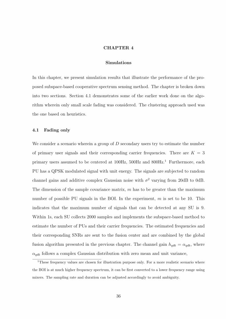
For different values of noise power, the percentage of correct detections is shown in

The dramatic increase in Pd is expected because missed detections usually occur due to

deep fading and/or noise uncertainty, and false alarms mainly due to noise uncertainty.

With the collaboration of multiple SUs, the chance of deep fading at all SUs (all SUs miss

the signal) is reduced dramatically. The dramatic increase in the probability of correct

detection is expected because with the collaboration of multiple SUs, the chance of deep

fading at all SUs reduces drastically. For different values of noise power, the percentage

of correct detections is shown in Fig. 4.1 with σ2 varying from 20dB to 0dB for one, five

and ten SUs.

0 5 10 15 200

0.1

0.2

0.3

0.4

0.5

0.6

0.7

0.8

0.9

1

σ2 (dB)

prob

abili

ty o

f cor

rect

det

ectio

n

1 user5 users10 users

Figure 4.1: The percentage of correct detections as a function of σ2 using one, five and

ten SUs, respectively. K = 3.

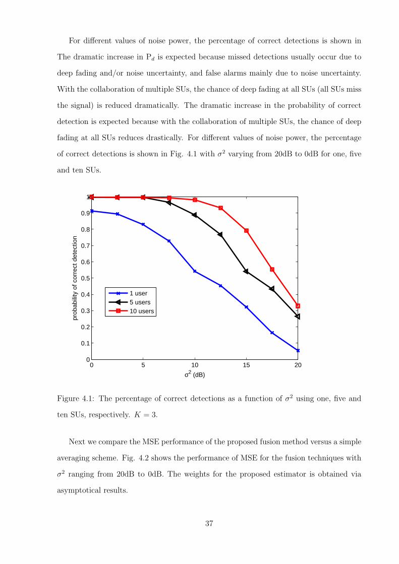
Next we compare the MSE performance of the proposed fusion method versus a simple

averaging scheme. Fig. 4.2 shows the performance of MSE for the fusion techniques with

σ2 ranging from 20dB to 0dB. The weights for the proposed estimator is obtained via

asymptotical results.

37

−20 −15 −10 −5 010

−6

10−5

10−4

10−3

10−2

10−1

100

1/σ2(dB)

MS

E(ω

1)

1 SUWeighted sum, 5 SUsWeighted sum, 10 SUsAverage, 5 SUsAverage, 10 SUs

Weighted Sum

Average

(a) MSE of estimation of ω1.

−20 −15 −10 −5 010

−6

10−5

10−4

10−3

10−2

10−1

100

1/σ2(dB)

MS

E(ω

2)


Weighted Sum

Average

(b) MSE of estimation of ω2.

−20 −15 −10 −5 010

−6

10−5

10−4

10−3

10−2

10−1

100

1/σ2(dB)

MS

E(ω

3)


Weighted Sum

Average

(c) MSE of estimation of ω3.

Figure 4.2: MSE performance as a function of 1/σ2 of all three PU signals using one,

five and ten SUs, respectively.MSE performance of all three fusion techniques. Number

of SUs collaborating is fixed at 10.

38

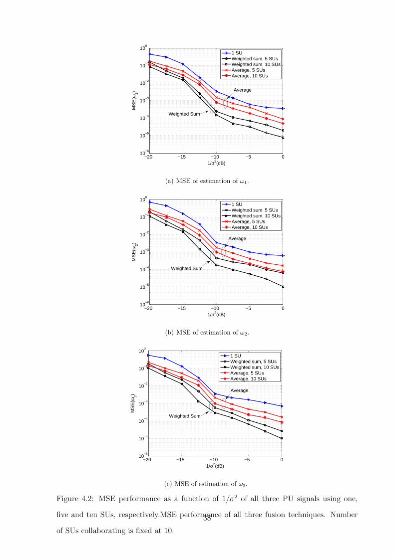
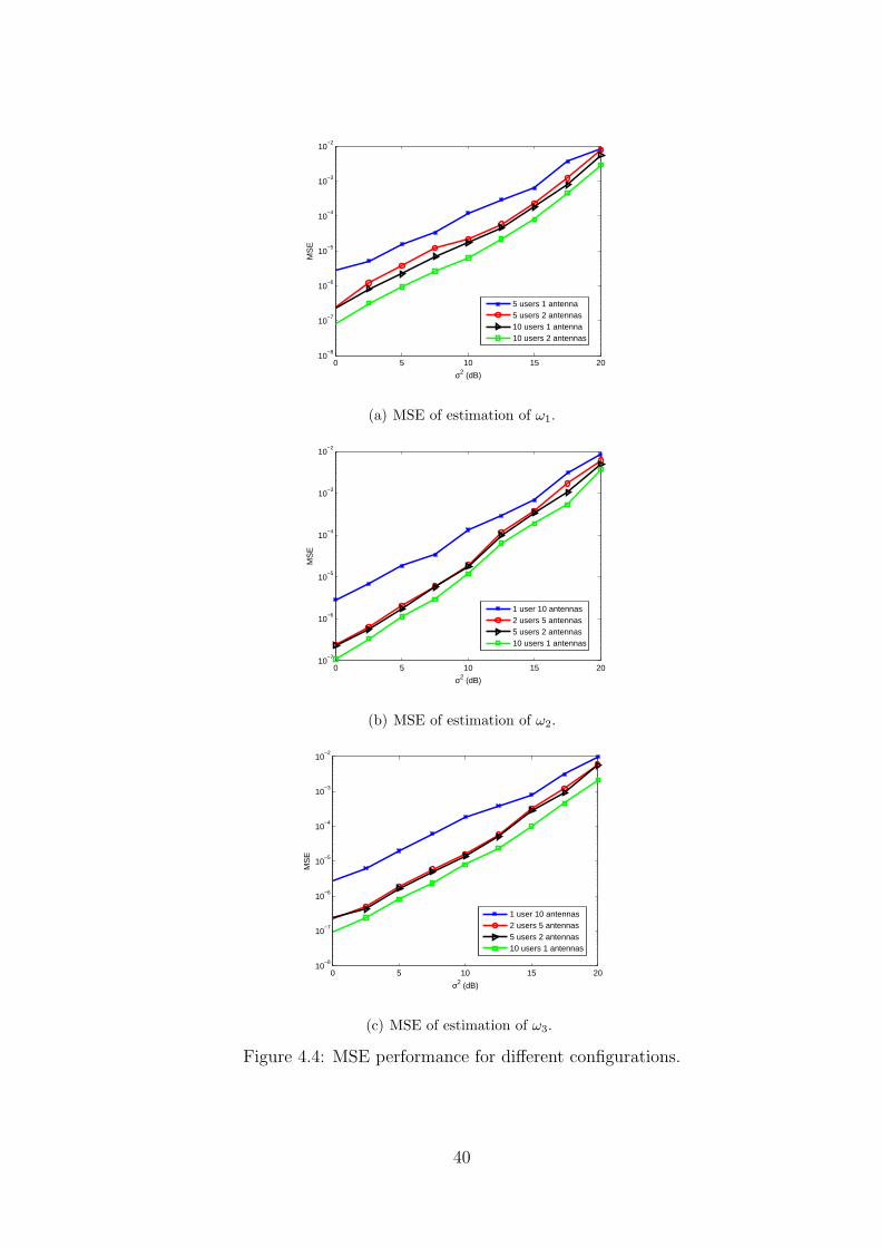
The extension of the results to the multiple antenna case provides different kind of

scenarios, with users having different number of antennas collaborating in a network trying

to find K and the corresponding ωk’s. The following set of figures show the performance

for many type of configurations (Fig. 4.3 and Fig. 4.4). From the figures the interesting

behavior to note is that when the total number of antennas are the same, the performance

tend to follow very close to each other. This is due to the absence of the shadowing effects.

The next section will reevaluate the performance of our systems under the dual effects of

shadowing and fading.

−20 −15 −10 −5 00

0.1

0.2

0.3

0.4

0.5

0.6

0.7

0.8

0.9

1

SNR in dB

p(µ)

1 SU 1 antenna1 SU 2 antennas5 SU 1 antenna5 SUs 2 antennas10 SUs 1 antenna10 SUs 2 antennas

Figure 4.3: The percentage of correct detections as a function of 1/σ2 for various config-

urations. K = 3.

4.2 Shadowing plus fading

We now consider three configurations: one secondary user equipped with ten antennas;

five secondary users each with two antennas; and ten secondary users each with one

antenna. Note that in all these configurations, the total number of antennas are fixed to

39

0 5 10 15 2010

−8

10−7

10−6

10−5

10−4

10−3

10−2

MS

E

σ2 (dB)

5 users 1 antenna5 users 2 antennas10 users 1 antenna10 users 2 antennas


0 5 10 15 2010

−7

10−6

10−5

10−4

10−3

10−2

MS

E

σ2 (dB)

1 user 10 antennas2 users 5 antennas5 users 2 antennas10 users 1 antennas


0 5 10 15 2010

−8

10−7

10−6

10−5

10−4

10−3

10−2

MS

E

σ2 (dB)

1 user 10 antennas2 users 5 antennas5 users 2 antennas10 users 1 antennas


Figure 4.4: MSE performance for different configurations.

40

be ten, implying that the same amount of data is collected for spectrum sensing. The first

configuration is a degenerated case where the fusion center is not required and one normal

eigendecomposition of the sample covariance matrix is sufficient for PU signal detection

and their carrier frequency estimation. Assume that, there are three PUs with their carrier

frequencies centered at 200Hz, 500Hz and 600Hz, respectively. 2 Both shadowing and

Rayleigh fading factors are considered in sensing, i.e., the channel gain hqdk = αqdkβqk,

where αqdk follows a complex Gaussian distribution with zero mean and unit variance,

and βqk is a log-normal random variable with the standard deviation of ρ dB.

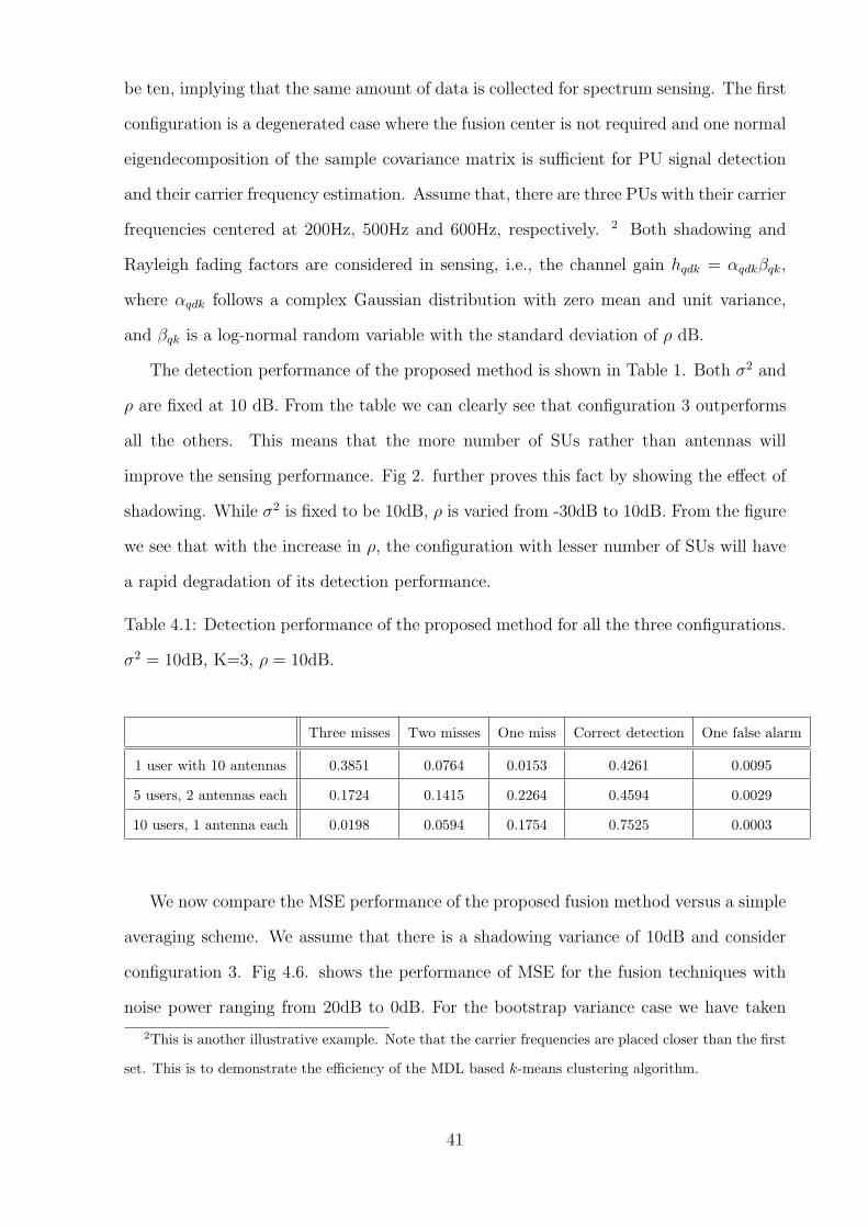
The detection performance of the proposed method is shown in Table 1. Both σ2 and

ρ are fixed at 10 dB. From the table we can clearly see that configuration 3 outperforms

all the others. This means that the more number of SUs rather than antennas will

improve the sensing performance. Fig 2. further proves this fact by showing the effect of

shadowing. While σ2 is fixed to be 10dB, ρ is varied from -30dB to 10dB. From the figure

we see that with the increase in ρ, the configuration with lesser number of SUs will have

a rapid degradation of its detection performance.

Table 4.1: Detection performance of the proposed method for all the three configurations.

σ2 = 10dB, K=3, ρ = 10dB.

Three misses Two misses One miss Correct detection One false alarm

1 user with 10 antennas 0.3851 0.0764 0.0153 0.4261 0.0095

5 users, 2 antennas each 0.1724 0.1415 0.2264 0.4594 0.0029

10 users, 1 antenna each 0.0198 0.0594 0.1754 0.7525 0.0003

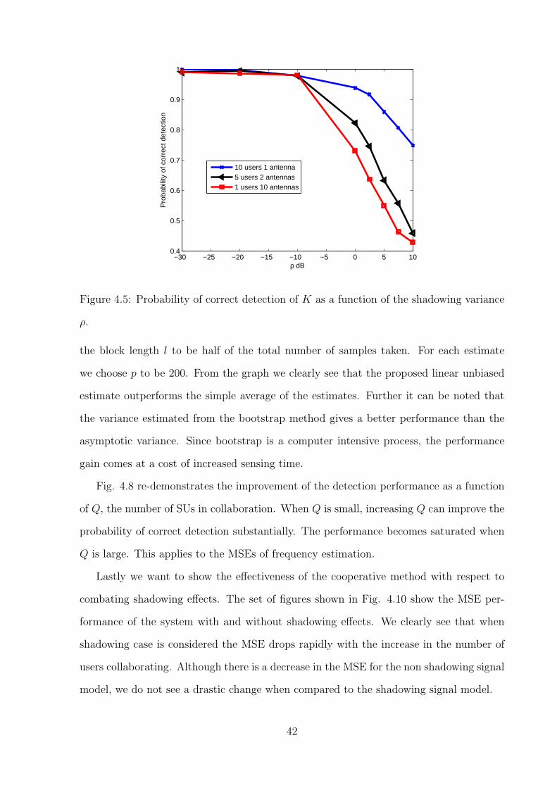
We now compare the MSE performance of the proposed fusion method versus a simple

averaging scheme. We assume that there is a shadowing variance of 10dB and consider

configuration 3. Fig 4.6. shows the performance of MSE for the fusion techniques with

noise power ranging from 20dB to 0dB. For the bootstrap variance case we have taken

2This is another illustrative example. Note that the carrier frequencies are placed closer than the first

set. This is to demonstrate the efficiency of the MDL based k-means clustering algorithm.

41

−30 −25 −20 −15 −10 −5 0 5 100.4

0.5

0.6

0.7

0.8

0.9

1

ρ dB

Pro

babi

lity

of c

orre

ct d

etec

tion

10 users 1 antenna5 users 2 antennas1 users 10 antennas

Figure 4.5: Probability of correct detection of K as a function of the shadowing variance

ρ.

the block length l to be half of the total number of samples taken. For each estimate

we choose p to be 200. From the graph we clearly see that the proposed linear unbiased

estimate outperforms the simple average of the estimates. Further it can be noted that

the variance estimated from the bootstrap method gives a better performance than the

asymptotic variance. Since bootstrap is a computer intensive process, the performance

gain comes at a cost of increased sensing time.

Fig. 4.8 re-demonstrates the improvement of the detection performance as a function

of Q, the number of SUs in collaboration. When Q is small, increasing Q can improve the

probability of correct detection substantially. The performance becomes saturated when

Q is large. This applies to the MSEs of frequency estimation.

Lastly we want to show the effectiveness of the cooperative method with respect to

combating shadowing effects. The set of figures shown in Fig. 4.10 show the MSE per-

formance of the system with and without shadowing effects. We clearly see that when

shadowing case is considered the MSE drops rapidly with the increase in the number of

users collaborating. Although there is a decrease in the MSE for the non shadowing signal

model, we do not see a drastic change when compared to the shadowing signal model.

42

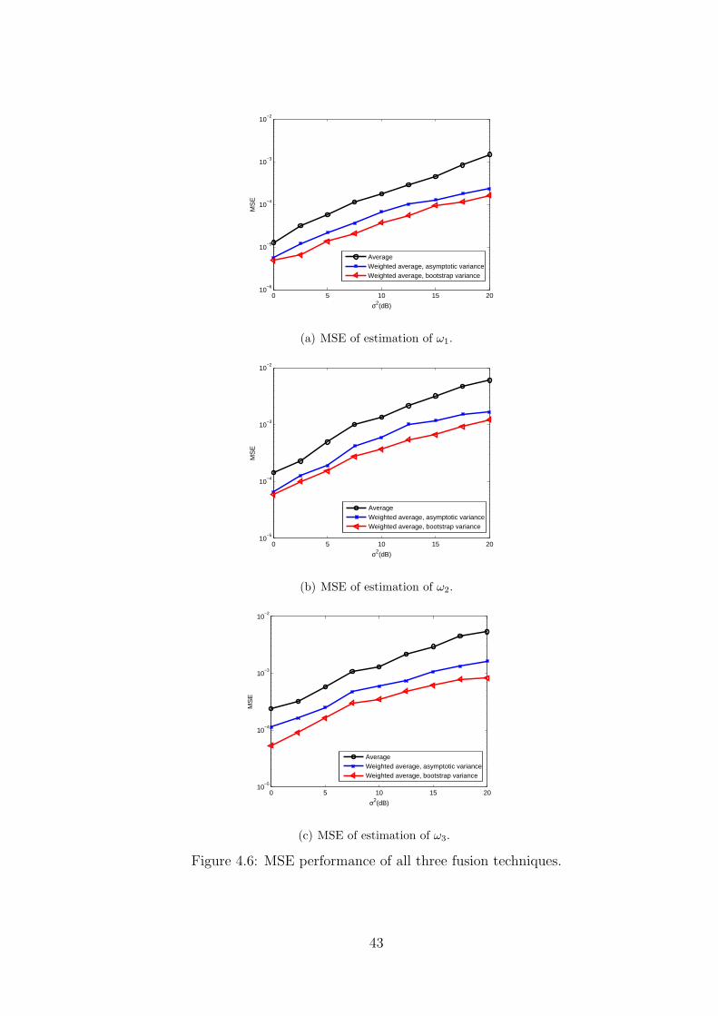
0 5 10 15 2010

−6

10−5

10−4

10−3

10−2

σ2(dB)

MS

E

AverageWeighted average, asymptotic varianceWeighted average, bootstrap variance


0 5 10 15 2010

−5

10−4

10−3

10−2

σ2(dB)

MS

E



0 5 10 15 2010

−5

10−4

10−3

10−2

σ2(dB)

MS

E



Figure 4.6: MSE performance of all three fusion techniques.

43

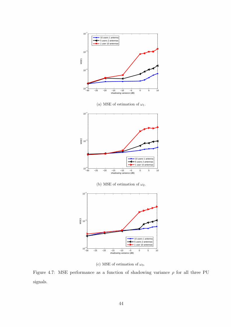
−30 −25 −20 −15 −10 −5 0 5 1010

−5

10−4

10−3

10−2

MS

E1

shadowing variance (dB)

10 users 1 antenna5 users 2 antennas1 user 10 antennas


−30 −25 −20 −15 −10 −5 0 5 1010

−4

10−3

10−2

MS

E2




−30 −25 −20 −15 −10 −5 0 5 1010

−4

10−3

10−2

MS

E3




Figure 4.7: MSE performance as a function of shadowing variance ρ for all three PU

signals.

44

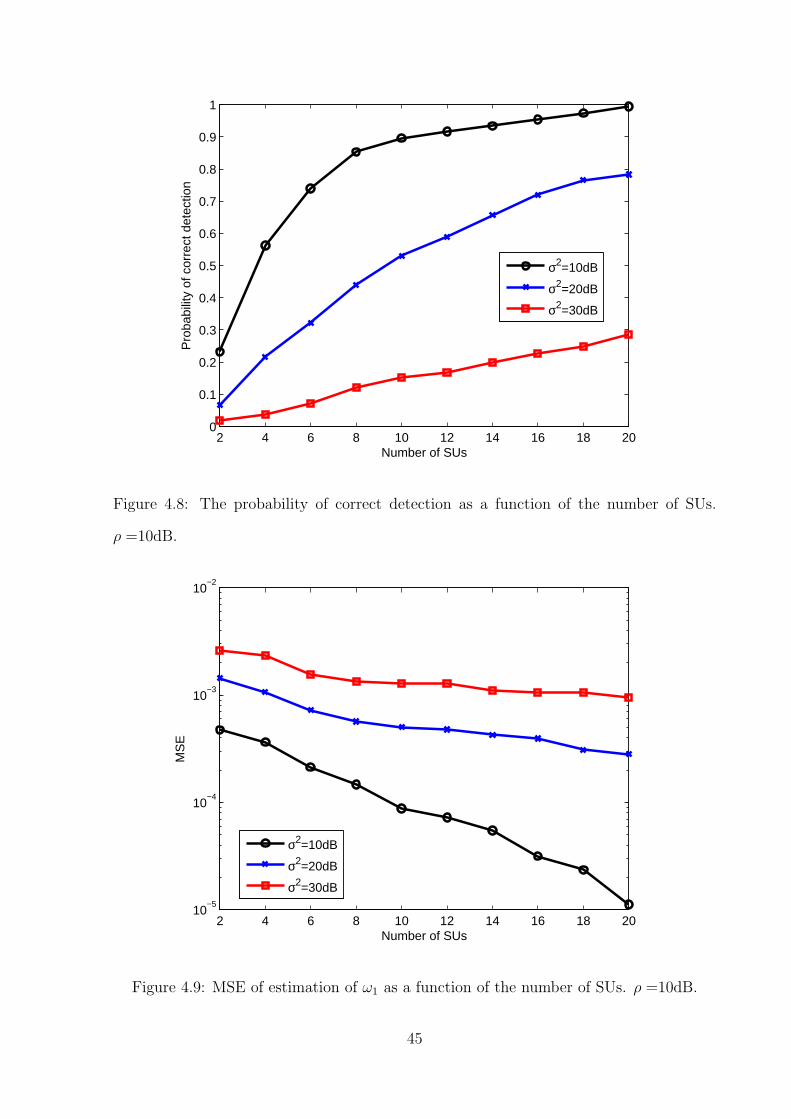
2 4 6 8 10 12 14 16 18 200

0.1

0.2

0.3

0.4

0.5

0.6

0.7

0.8

0.9

1

Number of SUs

Pro

babi

lity

of c

orre

ct d

etec

tion

σ2=10dB

σ2=20dB

σ2=30dB

Figure 4.8: The probability of correct detection as a function of the number of SUs.

ρ =10dB.

2 4 6 8 10 12 14 16 18 2010

−5

10−4

10−3

10−2

Number of SUs

MS

E

σ2=10dB

σ2=20dB

σ2=30dB

Figure 4.9: MSE of estimation of ω1 as a function of the number of SUs. ρ =10dB.

45

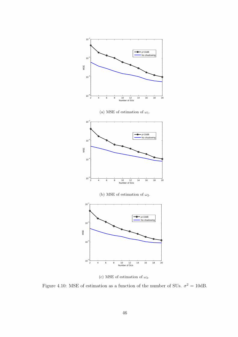
2 4 6 8 10 12 14 16 18 2010

−6

10−5

10−4

10−3

MS

E

Number of SUs

ρ=10dBNo shadowing


2 4 6 8 10 12 14 16 18 2010

−5

10−4

10−3

10−2

MS

E

Number of SUs

ρ=10dBNo shadowing


2 4 6 8 10 12 14 16 18 2010

−5

10−4

10−3

10−2

MS

E

Number of SUs

ρ=10dBNo shadowing


Figure 4.10: MSE of estimation as a function of the number of SUs. σ2 = 10dB.

46

CHAPTER 5

CONCLUSIONS

In this thesis we have proposed a subspace-based cooperative spectrum sensing technique,

where several SUs collaboratively determine the number of PUs in a wide BOI and their

carrier frequencies. At each SU, a preliminary estimate based on its own sample covariance

matrix is obtained using the subspace method. These estimates are then sent to a fusion

center. The problem of grouping the corresponding estimates from different secondary

users is addressed by using the MDL-based k-means algorithm. The local estimates

within the same groups are combined using an unbiased linear minimum mean square

estimator which can be reduced to a weighted sum of local estimates and the weights

are proportional to the inverse of the variances of these estimates. We further improve

the performance by estimating the variances using the bootstrap method on the collected

samples. The performance of the proposed algorithm is investigated under different system

configurations. The accuracy of detecting PUs and estimating their carrier frequencies in

the presence of shadowing can be significantly improve through the collaboration among

secondary users.

Since the communication between SUs and the fusion center is assumed to be ideal,

there is scope for future work by considering noisy and faded communication channels.

The issues to be worked on could be to see the performance degradation when non ideal

channels are considered and ways to tackle them. Another issue that needs to be con-

sidered is the bandwidth constraint on the control channel. By quantizing the frequency

estimates and weights we would put a bound on the accuracy of the values being commu-

nicated which will result in the reduction of the estimation performance. There is thus a

need to also study the tardeoff issues between bandwidth requirements and the estimation

performance.

47

APPENDIX A

Derivation of the elements of the Q matrix

The eigenvalue λi of the noise space, i = 1, . . . , r is essentially the energy of the noise

projected to the direction represented by the eigenvector ui of the noise space. Since Dq

antennas are used at each SU and it is equivalent to equal gain combining when calculating

the sample covariance matrix R, eigenvalue λi can be written as follows

λi =1

N −m+ 1

N−m+1∑

n=1

Dq∑

d=1

∥∥uHi wqd(n)

∥∥2

The mean of λi is given by

E(λi) = E

(1

N −m+ 1

N−m+1∑

n=1

Dq∑

d=1

∥∥uHi wqd(n)

∥∥2)

(o)=

Dq

N −m+ 1

N−m+1∑

n=1

E

(uHi wqd(n)w

Hqd(n)uj

)(A.1)

= Dqσ2

Equality at (o) is from the fact that the noise samples are independent of each other and

across the antennas.

The ijth elements in Ωr is Cov(λi, λj), which can be derived as follows

Cov(λi, λj) = E[(λi −Dqσ2)(λj −Dqσ

2)]

= E

[(1

N −m+ 1

N−m+1∑

n=1

Dq∑

d=1

∥∥uHi wqd(n)

∥∥2 −Dqσ2

)(A.2)

(1

N −m+ 1

N−m+1∑

s=1

Dq∑

b=1

∥∥uHj wqb(s)

∥∥2 −Dqσ2

)]

To simplify the notation, define vi(p)∆= uH

i wqd(n), p = 1, · · · , Dq(N − m + 1) and p =

48

(d− 1)(N −m+ 1) + n. Then, (A.2) becomes

Cov(λi, λj) = E

1

N −m+ 1

Dq(N−m+1)∑

p=1

‖vi(p)‖2 −Dqσ

2

1

N −m+ 1

Dq(N−m+1)∑

t=1

‖vj(t)‖2 −Dqσ

2

=1

(N −m+ 1)2

Dq(N−m+1)∑

p=1

Dq(N−m+1)∑

t=1

E

(‖vi(p)‖

2 ‖vj(t)‖2

)−

Dqσ2

N −m+ 1

Dq(N−m+1)∑

p=1

(E(‖vi(p)‖

2)+ E(‖vi(p)‖

2))+D2

qσ4

=1

(N −m+ 1)2

Dq(N−m+1)∑

p=1

Dq(N−m+1)∑

t=1

E(‖vi(p)‖

2 ‖vj(t)‖2)−D2

qσ4(A.3)

Consider E(‖vi(p)‖

2 ‖vj(t)‖2) in (A.3). It can be regarded as the expectation of the

product of four Gaussian random variables and each of them has zero mean. Then,

E

(‖vi(p)‖

2 ‖vj(t)‖2

)= E

(vi(p)v

∗i (p)vj(t)v

∗j (t)

)

= E

(vi(p)v

∗i (p)

)E

(vj(t)v

∗j (t)

)+ E

(vi(p)vj(t)

)E

(v∗i (p)v

∗j (t)

)+

E

(vi(p)v

∗j (t)

)E

(v∗i (p)vj(t)

)(A.4)

Plug (A.4) into (A.3) and we have three terms in the double summation.

The first term is

1

(N −m+ 1)2

Dq(N−m+1)∑

p=1

Dq(N−m+1)∑

t=1

E

(vi(p)v

∗i (p)

)E

(vj(t)v

∗j (t)

)= D2

qσ4

The second term is

1

(N −m+ 1)2

Dq(N−m+1)∑

p=1

Dq(N−m+1)∑

t=1

E

(vi(p)vj(t)

)E

(v∗i (p)v

∗j (t)

)

(a)=

1

(N −m+ 1)2

Dq(N−m+1)∑

p=1

Dq(N−m+1)∑

t=1

E

(uHi wqd(n)u

Hj wqb(s)

)E

(wH

qd(n)uiwHqb(s)uj

)

=1

(N −m+ 1)2

Dq(N−m+1)∑

p=1

Dq(N−m+1)∑

t=1

E

(uHi wqd(n)w

Tqb(s)u

∗j

)E

(uTi w

∗qd(n)w

Hqb(s)uj

)

(b)=0

49

Note that in (a) each index p corresponds to a unique pair of (d, n) and each index t

corresponds to a unique pair of (b, s). Equality at (b) is due to the independence of the

complex noise sequence and E[w2qd(n)] = 0.

The third term is

1

(N −m+ 1)2

(N−m+1)∑

p=1

(N−m+1)∑

t=1

E

(vi(p)v

∗j (t)

)E

(v∗i (p)vj(t)

)

=1

(N −m+ 1)2

Dq(N−m+1)∑

p=1

Dq(N−m+1)∑

t=1

E

(uHi wqd(n)w

Hqb(s)uj

)E

(uHj wqb(s)w

Hqd(s)ui

)

(A.5)

Since the expectations under the summation give nonzero values only when there is some

overlap between wqd(n) and wqb(s), i.e., they have common elements, (A.5) becomes

1

(N −m+ 1)2

Dq∑

d=1

N−m+1∑

n=1

n+m−1∑

s=n−m+1

E

(uHi wqd(n)w

Hqb(s)uj

)E

(uHj wqs(n)w

Hqb(s)ui

)

=Dqσ

4

N −m+ 1

(‖αij(0)‖

2 +m−1∑

p=1

(‖αij(p)‖

2 + ‖αji(p)‖2

))

where αij(p) = uHi J

puj. J is the m dimensional upper shift matrix with the (n,m)th

element Jn,m = δn+1,m with δij as the Kronecker delta symbol.

Combining all the results, the ijth element of Ωr becomes

Cov(λi, λj) = D2qσ

4 +D2

qσ4

N −m+ 1

‖αij(0)‖

2 +m−1∑

p=1

(‖αij(p)‖

2 + ‖αji(p)‖2

)−D2

qσ4

=D2

qσ4

N −m+ 1

‖αij(0)‖

2 +m−1∑

p=1

(‖αij(p)‖

2 + ‖αji(p)‖2

)(A.6)

Using (A.6) we can construct the covariance matrix Ωr. For implementation the noise

variance can be estimated the r-smallest eigenvalues of R for selected value of r

Dqσ2 =

1

r

r−1∑

i=0

λm−i (A.7)

ui and uj, i, j = 1, · · · , r can be approximated by the corresponding r eigenvectors of R.

The normalized sum square of the last r eigenvalues can be constructed for the Chi-square

test. The complete test procedure can be summarized as follows:

Given the data Zq(1), · · · ,Zq(N) , estimate the order-m autocorrelation matrix R

50

using (??); perform the eigendecomposition of this matrix and order its eigenvalues λi

by decreasing values and the eigenvectors accordingly. Then for r = m,m− 1,m− 2, · · ·

• estimate the noise variance using (A.7)

• build an estimate of (λr − µr):

[λm−r+1 −Dqσ

2, λm−r+2 −Dqσ2, · · · , λm −Dqσ

2]

• estimate its covariance matrix Ωr, using (A.6).

• combining all the relations compute γr:

γr =N −m+ 1

D2q σ

4(λr − µr)

HΩr(λr − µr)

and compare it to tr; if γr > tr then go to next r; if γr ≤ tr then stop and choose

m− K = r. The threshold tr , read from a chi-square table, is chosen to achieve a

given probability of underestimating m− K.

51

APPENDIX B

Analysis of ESPRIT

Consider the following prepositions:

Proposition 1 : APAHG1 = G1Λ1, with Λ1 = Λ1−σ2I where Λ1 = diag[λ1, λ2, · · · , λK ].

Proof : Multiplying (3.3) by G1 on both sides we get

RG1 = G1Λ1 = APAHG1 +G1σ2I

APAHG1 = G1(Λ1 − σ2I) = G1Λ1

Proposition 2 : G1 = AC where C = PAHG1Λ−1

1 and C−1 = GH1 A.

Proof : This can be obtained by using proposition 1.

Let

A1 = [Im−1 0]A

A2 = [0 Im−1]A (B.1)

We can see that A2 = A1D where D = diag[ejω1 , ejω2 , · · · , ejωK ]. From proposition 2 we

see that

F2 = A2C => F2 = A1DC = F1C−1DC = F1ψ

ψ = C−1DC and ψ = (FH1 F1)

−1FH1 F2

The structure of ψ clearly suggests that its eigenvalues will be the set to ωiKi=1.

52

APPENDIX C

Tracy-Widom distribution

The Tracy-Widom distribution can be expressed via the solution to the Painleve II dif-

ferential equation. Fβ can be explicitly given by

F2(s) = exp

(−

∫ ∞

s

(x− s)q2(s)dx

),

F1(s) = exp

(−1

2

∫ ∞

s

q(x)dx

)[F2(s)]

1/2

Here q(s) is the unique solution to the Painleve II differential equation

q = sq + 2q3 + α with α = 0,

satisfying the boundary condition

q(s) ∼ Ai(s), s → ∞,

where Ai(s) denotes the Airy function. Lot of programming has been done in Matlab

to help come up with a solution to the Painleve II differential equation and evaluate the

Tracy- Widom distributions. This allowed the tabulation of the Tracy Widom distribu-

tions, particularly for β = 1, 2, 4. The detailed tabulations can be found in [75]. This can

be used for statistical look-up use. The Tracy Widom density function is as shown in Fig.

53

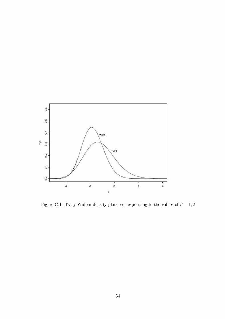
Figure C.1: Tracy-Widom density plots, corresponding to the values of β = 1, 2

54

APPENDIX D

More on k-means clustering technique using the MDL principle

In section 3.3.1 an unsupervised clustering algorithm was presented which helps k-means

algorithm learn the number of clusters in an iterative approach. This appendix aims at

providing more information on the basis of k-means algorithm and how the MDL principle

is used to arrive at the optimum number of clusters. The algorithm provided in section

3.3.1 just provides the basic framework without specifying the details about the coding

procedures for the indices and the errors. We conclude this appendix by providing the

encodings for the index and error terms.

D.1 k-means

k-means is a type of clustering algorithm which breaks an n length data set into k subsets,

where the members of each of the k subset is closest to a mean ck. Thus if we have a d

dimensional data set X = x1, x2, · · · , xn, the k-means algorithms breaks the set S into

k (k < n) subsets S = S1,S2, · · · ,Sksuch that

minS

∑

i=1

k∑

xj∈Si

‖xj − ci‖2

where ci is called the mean of Si. The method has a requirement of having a decision

on the number of clusters in advance, and if the result is not correct, we tend to get

very different clustering results. This property of the k means algorithms is illustrated

in [68] through simulations. Fig. B.1 illustrates what happens if we take a simple cluster

structure (five clusters (30 points) and two isolated points) and initialize k-means with

the wrong number of centers. The figure shows how dependent the results are on the

initializations.

Since many of the applications do not have the knowledge of the number of clusters

55

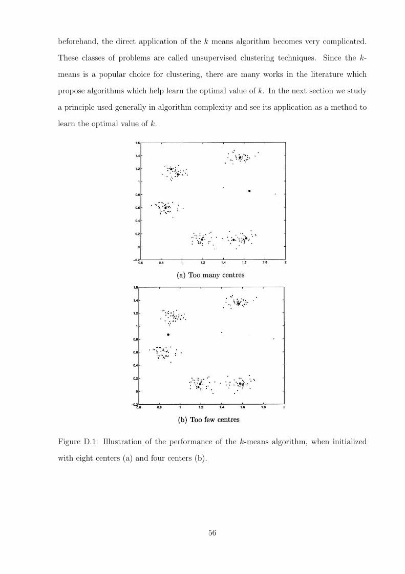
beforehand, the direct application of the k means algorithm becomes very complicated.

These classes of problems are called unsupervised clustering techniques. Since the k-

means is a popular choice for clustering, there are many works in the literature which

propose algorithms which help learn the optimal value of k. In the next section we study

a principle used generally in algorithm complexity and see its application as a method to

learn the optimal value of k.

Figure D.1: Illustration of the performance of the k-means algorithm, when initialized

with eight centers (a) and four centers (b).

56

D.2 MDL principle

The minimum description length principle, introduced by Jorma Rissanen in 1978, is

obtaining the best hypothesis on a set of data which leads to the maximum compression

of the data set. Any data set can be represented by symbols. If the binary representation

of the data is considered, the aim of the MDL principle is to find any regularities in the

data set which can be used to reduce the number of bits required to represent them.

Therefore, if we know that the data set follows the property of being in cluster sets, then

the MDL principle becomes analogous to differential encoding. To compress the data we

can now assign reference data points and the data points are encoded by the reference

vector index and the error. This would obviously require lesser bits than encoding each

data point separately. The MDL principle avoids overfitting of data since it not only

considers the complexity of the data set given the hypothesis but also the hypothesis

itself. The algorithm in section 3.3.1 thus treats the cluster space as a network and starts

off with an overly complex network (having a lot of cluster centers). It then uses MDL

as a pruning technique and to identify estimates from false alarms termed as outliers,

gradually reducing the number of redundant cluster centers until it arrives at a point

which balances the error versus the number of cluster centers.

D.3 Instantiations of the MDL-Algorithm

The iterative algorithm can be represented by the flow graph shown in Fig. B.2. The

clustering problem is approached as a minimization of the length of the description of the

data set D through vector quantization. If the outliers are already identified as the set

B, then I = D − B is the data set which needs to described by the cluster centers D.

The length of encoding D by using the set C is given by

L(D(C)) = L(D) + L(I(C)) + L(ǫ(IC)) + L(B) (D.1)

We see that the length of encoding the data set is the sum of encoding the cluster center

set D, the length of encoding the frequency estimates using C, the sum of the residual

57

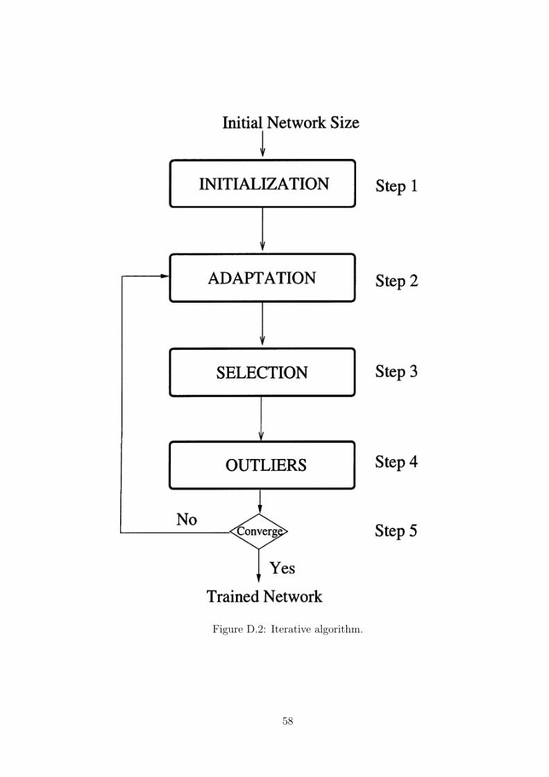
Figure D.2: Iterative algorithm.

58

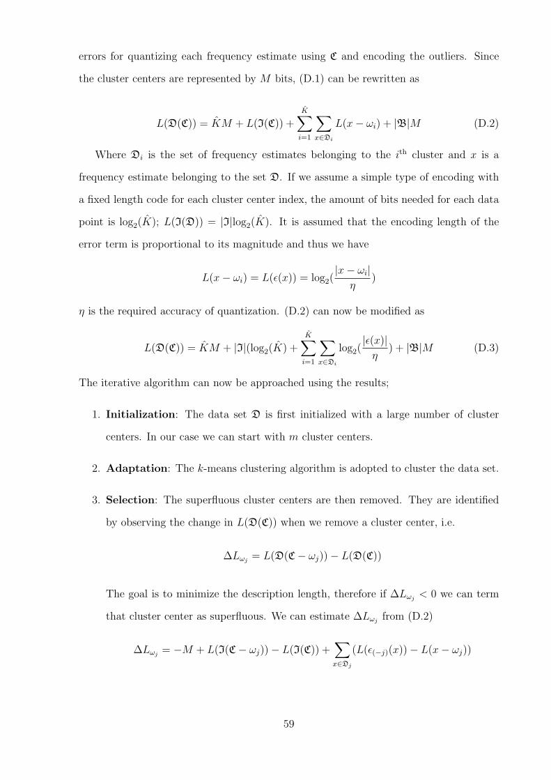
errors for quantizing each frequency estimate using C and encoding the outliers. Since

the cluster centers are represented by M bits, (D.1) can be rewritten as

L(D(C)) = KM + L(I(C)) +K∑

i=1

∑

x∈Di

L(x− ωi) + |B|M (D.2)

Where Di is the set of frequency estimates belonging to the ith cluster and x is a

frequency estimate belonging to the set D. If we assume a simple type of encoding with

a fixed length code for each cluster center index, the amount of bits needed for each data

point is log2(K); L(I(D)) = |I|log2(K). It is assumed that the encoding length of the

error term is proportional to its magnitude and thus we have

L(x− ωi) = L(ǫ(x)) = log2(|x− ωi|

η)

η is the required accuracy of quantization. (D.2) can now be modified as

L(D(C)) = KM + |I|(log2(K) +K∑

i=1

∑

x∈Di

log2(|ǫ(x)|

η) + |B|M (D.3)

The iterative algorithm can now be approached using the results;

1. Initialization: The data set D is first initialized with a large number of cluster

centers. In our case we can start with m cluster centers.

2. Adaptation: The k-means clustering algorithm is adopted to cluster the data set.

3. Selection: The superfluous cluster centers are then removed. They are identified

by observing the change in L(D(C)) when we remove a cluster center, i.e.

∆Lωj= L(D(C− ωj))− L(D(C))

The goal is to minimize the description length, therefore if ∆Lωj< 0 we can term

that cluster center as superfluous. We can estimate ∆Lωjfrom (D.2)

∆Lωj= −M + L(I(C− ωj))− L(I(C)) +

∑

x∈Dj

(L(ǫ(−j)(x))− L(x− ωj))

59

where ǫ(−j)(x) is the error caused by the vector x when ωj is removed from C, i.e.,

ǫ(−j)(x) = (x−ωk), k = arg mini=1,··· ,j−1,j+1,··· ,K ‖x− ωi‖. The above term can now

be expressed using (D.3) as

∆Lωj= M + |I|(log2(K − 1)− log2(K)) +

∑

x∈Dj

log2

(|ǫ(−j)(x)|

|ǫ(x)|

)(D.4)

4. Outliers: According to the MDL principle, those estimates are termed to be outliers

which can be encoded with less bits directly rather than a reference vector quantizing

them. This can be easily calculated from (D.1) by checking the change in the coding

length when a data point y ∈ Di is termed as an outlier.

K < L((I− y)(C)) + L(y − ωi) + F|Di|=1M (D.5)

where

F|Di|=1 =

1 : |Di| = 1

0 : otherwise

is the indicator function, indicating if y is the only data point in cluster i.

5. Convergence: If there were no outliers detected nor any cluster centers were re-

moved and the changes in the adaptation step were too small then we decide to

stop. Otherwise we goto step 2.

60

BIBLIOGRAPHY

[1] I. F. Akyildiz, W. Lee, M. C. Vuran, S. Mohanty, “Next generation/dynamic spec-

trum access/cognitive radio wireless networks: A survey,” Computer Networks Jour-

nal, vol. 50, pp. 2127-2159, May 2006.

[2] M. A. McHenry, “NSF Spectrum Occupancy Measurements Projects Summary,”

Shared Spectrum Company Report, Aug. 2005.

[3] S. Haykin,“Cognitive radio: Brain Empowered Wireless Communications,” IEEE

Journal Selet. Area on Communications, vol. 23, no. 2, pp. 201-220, Feb. 2005.

[4] I. Mitola, J. and J. Maguire, G. Q.,“Cognitive radio: making software radios more

personal,” IEEE Personal Commun. Mag., vol. 6, no. 4, pp. 13-18, Aug. 1999.

[5] J. G. Proakis,” Digital Communications, 4th ed. McGraw-Hill, 2001.

[6] R. Tandra and A. Sahai,“Fundamental limits on detection in low SNR under noise

uncertainty,” in Proc. IEEE Int. Conf. Wireless Networks, Commun. and Mobile

Computing, vol. 1, Pacific Grove, California, USA, Nov. 2004, pp. 772-776.

[7] A. V. Oppenheim, R. W. Schafer and J. R. Buck,” Discrete-Tme Signal Processing,

Prentice Hall, 1999.

[8] H. Urkowitz, “Energy detection of unknown deterministic signals,” Proc. IEEE, vol.

55, pp. 523-531, Apr. 1967.

[9] A. Sahai, N. Hoven, R. Tandra, “Some Fundamental Limits on Cognitive Radio,”

Proc. of Allerton Conference, Monticello, Oct 2004.

[10] U. Gardner, WA, “Exploitation of spectral redundancy in cyclostationary signals,”

IEEE Signal Processing Mag., vol. 8, no. 2, pp. 14-36, 1991.

61

[11] K. Kim, I. A. Akbar, K. K. Bae, J. Urn, C. M. Spooner and J. H. Reed, “Cyclosta-

tionary Approaches to Signal Detection and Classification in Cognitive Radio,” IEEE

International Symposium on New Frontiers in Dynamic Spectrum Access Networks,

2007.

[12] J. Lunden, V. Koivunen, A. Huttunen and H. V. Poor, “Spectrum sensing in cog-

nitive radios based on multiple cyclic frequencies,” 2nd International Conference on

Cognitive Radio Oriented Wireless Networks and Communications, Orlando, FL, Jul.

2007.

[13] B. Zayen, A. Hayar and D. Nussbaum, “Blind spectrum sensing for cognitive radio

based on model selection,” IEEE CrownCom, May 2008.

[14] Y. Zeng, Y.C. Liang, “Maximum-Minimum Eigenvalue Detection for Cognitive Ra-

dio,” in 18th Annual IEEE International Symposium on Personal, Indoor and Mobile

Radio Communication (PIMRC), pp. 1-5, Sept. 2007.

[15] Y. Zeng, Y.C. Liang, “Eigenvalue based Spectrum Sensing Algorithms for Cognitive

Radio,” arXiv:0804.2960

[16] F. Penna, R. Garello, M. A. Spirito, “Cooperative Spectrum Sensing based on the

Limiting Eigenvalue Ratio Distribution inWishart Matrices,”accepted for publication

in IEEE Comm. Letters, 2009.

[17] Y. Zeng and Y. Liang, “Covariance based signal detections for cognitive radio,” in

Proc. IEEE DySpan07, pp. 202-207, Apr. 2007.

[18] Sung Sue Hwang, Dong Chan Park, Suk Chan Kim, Myung Sun Song,Sun Min

Lim, “Spectrum sensing using Bussgang theorem for IEEE 802.22 WRAN,” in Proc.

Military Communications Conference, 2008. MILCOM 2008. IEEE, pp. 1-5, Nov.

2008.

[19] J.J. Bussgang, “Cross-correlation function of amplitude-distorted gaussian signals,”

Res. Lab. Elec., Mas. Inst. Technol., Cambridge MA, Tech. Rep. 216, Mar. 1952.

62

[20] H. Li, C. Li, and H. Dai, “Quickest spectrum sensing in cognitive radio,” in Proc. of

CISS’08, pp. 203- 208, Mar. 2008.

[21] Fehske, A. and Gaeddert, J. and Reed, J.H., “A new approach to signal classification

using spectral correlation and neural networks,” New Frontiers in Dynamic Spectrum

Access Networks, 2005. DySPAN 2005. 2005 First IEEE International Symposium

on, vol., no.pp. 144- 150, 8-11 Nov. 2005.

[22] Farhang-Boroujeny B. , “Filter Bank Spectrum Sensing for Cognitive Radios,” Signal

Processing, IEEE Transactions, Vol. 56, No. 5, pp.1801-1811, May 2008.

[23] Z. Quan, S. Cui, A.H. Sayed, and H.V. Poor, “Wideband spectrum sensing in cog-

nitive radio networks,” in Proc. IEEE Int. Communications Conf., Beijing, China,

May 2008, pp. 901-906.

[24] A. Taherpour, S. Gazor, and M. Nasiri-Kenari, “Wideband spectrum sensing in un-

known white Gaussian noise,” Special issue on Cognitive Spectrum Access in IET

Communications, Vol. 2, No. 6, pp.763-771, 2008.

[25] Z. Tian and G. B. Giannakis, “A wavelet approach to wideband spectrum sensing for

cognitive radios,” 1st Int. Conference on Cognitive Radio Oriented Wireless Networks

and Communications, Jun. 2006.

[26] Y. Hur, J. Park, W. Woo, K. Lim, C.-H. Lee, H. S. Kim and J. Laskar, “A wide-

band analog multi-resolution spectrum sensing technique for cognitive radio sys-

tems,” IEEE International Symposium on Circuits and Systems, May 2006.

[27] A. Ghasemi and E. S. Sousa, “Collaborative spectrum sensing for opportunistic access

in fading environments,” 1st IEEE Symp. New Frontiers in Dynamic Spectrum Access

Networks, Baltimore, USA, Nov. 2005,

[28] D. Cabric, A. Tkachenko, and R. Brodersen, “Spectrum sensing measurements of

pilot, energy, and collaborative detection,” in Proc. IEEE Military Commun. Conf.,

Washington, D.C., USA, Oct. 2006, pp. 17.

63

[29] X. Liu and S. Shankar, “Sensing-based opportunistic channel access,” Mobile Net-

works and Applications, vol. 11, no. 4, pp. 577-591, 2006.

[30] P. Pawetczak, G. J. Janssen, and R. V. Prasad, “Performance measures of dynamic

spectrum access networks,” in Proc. IEEE Global Telecomm. Conf. (Globecom), San

Francisco, California, USA, Nov./Dec. 2006.

[31] A. Ghasemi and E. S. Sousa, “Asymptotic performance of collaborative spectrum

sensing under correlated log-normal shadowing,” IEEE Commun. Lett., vol. 11, no.

1, pp. 34-36, Jan. 2007.

[32] E. Peh and Y.-C. Liang, “Optimization for cooperative sensing in cognitive radio

networks,” in Proc. IEEE Wireless Commun. and Networking Conf., Hong Kong,

Mar. 2007, pp. 27-32.

[33] E. Visotsky, S. Kuffner, and R. Peterson, “On collaborative detection of TV trans-

missions in support of dynamic spectrum sharing,” in Proc. IEEE Int. Symposium on

New Frontiers in Dynamic Spectrum Access Networks, Baltimore, Maryland, USA,

Nov. 2005, pp. 338-345.

[34] T. Weiss, J. Hillenbrand, and F. Jondral, “A diversity approach for the detection

of idle spectral resources in spectrum pooling systems,” in Proc. of the 48th Int.

Scientific Colloquium, Ilmenau, Germany, Sept.2003, pp. 37-38.

[35] S.M. Mishra, A. Sahai and R.W. Brodersen, “Cooperative Sensing among Cognitive

Radios,” IEEE International Conference on Communications, June 2006.

[36] J. Lunden, V. Koivunen, A. Huttunen, and H. V. Poor, “Spectrum sensing in cogni-

tive radios based on multiple cyclic frequencies,” in Proc. IEEE Int. Conf. Cognitive

Radio Oriented Wireless Networks and Commun. (Crowncom), Orlando, Florida,

USA, July/Aug. 2007.

[37] Z. Chair and P. K. Varshney, “Optimal data fusion in multiple sensor detection

systems,” IEEE Trans. Aerosp. Electron. Syst., vol. 22, no. 1, pp. 98-101, Jan. 1986.

64

[38] M. Gandetto, A. F. Cattoni, and C. S. Regazzoni, “A distributed approach to mode

identification and spectrum monitoring for cognitive radios,” in Proc. SDR Forum

Technical Conference, Orange County, California, USA, Nov. 2005..

[39] M. Gandetto, A. F. Cattoni, M. Musso, and C. S. Regazzoni, “Distributed coop-

erative mode identification for cognitive radio applications,” in Proc. International

Radio Science Union (URSI), New Delhi, India, Oct. 2005.

[40] A. F. Cattoni, I. Minetti, M. Gandetto, R. Niu, P. K. Varshney, and C. S. Regazzoni,

“A spectrum sensing algorithm based on distributed cognitive models,” in Proc. SDR

Forum Technical Conference, Orlando, Florida, USA, Nov. 2006..

[41] M. Gandetto and C. Regazzoni, “Spectrum sensing: A distributed approach for

cognitive terminals,” IEEE J. Select. Areas Commun., vol. 25, no. 3, pp. 546-557,

Apr. 2007.

[42] G. Shafer, “A Mathematical Theory of Evidence. Princeton, New Jersey, USA:

Princeton Univ. Press, 1976.

[43] P. Qihang, Z. Kun, W. Jun, and L. Shaoqian, “A distributed spectrum sensing scheme

based on credibility and evidence theory in cognitive radio context,” in Proc. IEEE

Int. Symposium on Personal, Indoor and Mobile Radio Commun., Helsinki, Finland,

Sept. 2006, pp. 15.

[44] P. Paweczak, G. J. Janssen, and R. V. Prasad, “Performance measures of dynamic

spectrum access networks,” Proc. IEEE Global Telecomm. Conf. (Globecom), vol. 25,

no. 3, pp. 546-557, Apr. 2007. San Francisco, California, USA, Nov./Dec. 2006.

[45] E. Visotsky, S. Kuffner, and R. Peterson, “On collaborative detection of TV trans-

missions in support of dynamic spectrum sensing,” Proc. IEEE Symp. New Frontiers

in Dynamic Spectrum Access Networks (Baltimore, USA), pp. 338-345, Nov. 811,

2005.

65

[46] C. Sun, W. Zhang, and K. B. Letaief, “Cooperative spectrum sensing for cognitive

radios under bandwidth constraints,” in Proc. IEEE Wireless Commun. and Net-

working Conf, Hong Kong, Mar. 2007, pp. 15.

[47] M. Gandetto, A. F. Cattoni, and C. S. Regazzoni, “A distributed approach to mode

identification and spectrum monitoring for cognitive radios,” in Proc. SDR Forum

Technical Conference, Orange County, California, USA, Nov. 2005.

[48] M. Gandetto, A. F. Cattoni, M. Musso, and C. S. Regazzoni, “Distributed coop-

erative mode identification for cognitive radio applications,” in Proc. International

Radio Science Union (URSI), New Delhi, India, Oct. 2005.

[49] M. Gandetto and C. Regazzoni, “Spectrum sensing: A distributed approach for

cognitive terminals,” IEEE J. Select. Areas Commun., vol. 25, no. 3, pp. 546-557,

Apr. 2007.

[50] A. Ghasemi and E. Sousa, “Collaborative spectrum sensing for opportunistic access in

fading environments,” in Proc. IEEE Int. Symposium on New Frontiers in Dynamic

Spectrum Access Networks, Baltimore, Maryland, USA, Nov. 2005, pp. 131-136.

[51] Wei Zhang, Mallik.R.K., Ben Letaief. K., “Cooperative spectrum sensing in cognitive

radio networks,” in PProc. IEEE Int. Symposium on New Frontiers in Dynamic


[52] N. Ahmed, D. Hadaller, and S. Keshav, “GUESS: gossiping updates for efficient

spectrum sensing,” in Proc. International workshop on Decentralized resource sharing

in mobile computing and networking, Los Angeles, California, USA, 2006, pp. 12-17.

[53] B. Wild and K. Ramchandran, “Detecting primary receivers for cognitive radio ap-

plications,” in PProc. IEEE Int. Symposium on New Frontiers in Dynamic Spectrum

Access Networks, Proc. IEEE Int. Symposium on New Frontiers in Dynamic Spec-

trum Access Networks,

66

[54] S. Shankar, C. Cordeiro, and K. Challapali, “Spectrum agile radios: utilization and

sensing architectures,” in Proc. IEEE Int. Symposium on New Frontiers in Dynamic


[55] Standard for Wireless Regional Area Networks (WRAN) - Specific requirements -

Part 22: Cognitive Wireless RAN Medium Access Control (MAC) and Physical Layer

(PHY) Specifications: Policies and procedures for operation in the TV Bands, The

Institute of Electrical and Electronics Engineering, Inc. Std. IEEE 802.22.

[56] R. Rao, Q. Cheng and P. Ray, “Subspace-based Cooperative Spectrum Sensing for

Cognitive Radio,” in Proc. 42nd Annual Asilomar Conference on Signals, Systems,

and Computers, Pacific Grove, CA, Oct. 2008.

[57] A. Sahai and D. Cabric, “Spectrum sensing: fundamental limits and practical chal-

lenges,” IEEE International Symposium on New Frontiers in Dynamic Spectrum

Access Networks, Nov. 2005.

[58] Z. Quan, S. Cui, A. Sayed and H. V. Poor, “Wideband Spectrum Sensing in Cognitive

Radio Networks,” ICC, May, 2008.

[59] A. Wagstaff and N. Merricks, “A Subspace-Based Method for Spectrum Sensing,”

2007.

[60] A. Ghasemi and E. S. Sousa, “Collaborative spectrum sensing for opportunistic access

in fading environments,” 1st IEEE Symp. New Frontiers in Dynamic Spectrum Access

Networks, Baltimore, USA, Nov. 2005,

[61] S.M. Mishra, A. Sahai and R.W. Brodersen, “Cooperative Sensing among Cognitive

Radios,” IEEE International Conference on Communications, June 2006.

[62] J. Unnikrishnan and V.V. Veeravalli, “Cooperative Sensing for Primary Detection in

Cognitive Radio,” IEEE Journal of Selected Topics in Signal Processing, Vol. 2, No.

1, pp. 18-27, Feb. 2008.

67

[63] T.S. Rappaport, Wireless Communications: Principles and Practice. Prentice Hall,

2002.

[64] R. Roy and T. Kailath, “ESPRIT-estimation of signal parameters via rotational

invariance techniques,” IEEE Trans. on Acoustics, Speech, and Signal Processing,

Vol. 37, No. 7, pp. 984-995, Jul 1989.

[65] P. Stoica and T. Soderstrom, “Statistical Analysis of MUSIC and Subspace Rotation

Estimates of Sinusoidal Frequencies,” IEEE Trans. Signal Processing, vol. 39, no. 8,

pp 1836-1847, 1991.

[66] J.-J. Fuchs, “Estimating the number of sinusoids in additive white noise,” IEEE

Trans. on Signal Processing, vol. 36, no. 12, pp. 1846-1853, Dec. 1988.

[67] S. M. Kay, Fundamentals of Statistical Signal Processing, Vol. I - Estimation Theory,

Prentice Hall, 1993.

[68] Horst Bischof, Ales Leonardis and Alexander Selb, “ MDL Principle for Robust

Vector Quantization, ” Pattern Analysis and Application 2, (1999) (1), pp. 59-72.

[69] J. Rissanen, “Universal coding, information, prediction, and estimation, ” IEEE

Transactions on Information Theory, pp. 629-636, 1984.

[70] J. Rissanen, “Stochastic Complexity in Statistical Inquiry, ” Series in Computer

Science, Vol-15, 1989.

[71] Jun Shao and Dongsheng Tu. The Jackkinfe and Bootstrap, Springer Series in Statis-

tics,

[72] S. Kritchman and B. Nadler. “Determining the number of components in a factor

model from limited noisy data, ”Chem. Int. Lab. Sys.,2008.

[73] I.M. Johnstone,On the distribution of the largest eigenvalues in principal components

analysis, ”Annals of Statistics, vol. 29, pp. 295-327, 2001.

68

[74] M. Inaba, N. Katoh , H. Imai, “Applications of weighted Voronoi diagrams and ran-

domization to variance-based k-clustering,” 10th ACM Symposium on Computational

Geometry, pp. 332-339, 1994.

[75] A. Bejan, “ Tracy-Widom and Painleve II : computational aspects and realization in

S-Plus, in Proc. ”14th Conference on Applied and Industrial Mathematics, Chisinau,

Moldova, 2006.

69

VITA

Raghavendra U Rao

Candidate for the Degree of

Master of Science

Thesis: SUBSPACE-BASED COOPERATIVE SPECTRUM SENSING FOR COGNI-TIVE RADIOS

Major Field: Electrical Engineering

Biographical:

Personal Data:Born in Bangalore, Karnataka, India on December 28, 1984.

Education:Received the B.E. degree from Vishveshwaraya Technological University, Ban-galore, Karnataka, India, 2006, in TelecommunicationCompleted the requirements for the degree of Master of Science with a majorin Electrical Engineering Oklahoma State University in May, 2010.

Experience:Worked as Research Assistant at the Statistical Signal Processing Lab underDr. Qi Cheng from January 2008 to May 2010. He was the teaching assistantfor the course “Stochastic System” in Fall 2009.Before joining Oklahoma State University he worked in Infosys TechnologiesLtd., India as a software engineer. He was also a summer intern as an embeddedsoftware engineer at Gramin International, Kansas over the summer of 2008.

Publications:R. Rao, Q. Cheng and P. Ray, “Subspace-based Cooperative Spectrum Sensingfor Cognitive Radio,” in Proc. 42nd Annual Asilomar Conference on Signals,Systems, and Computers, Pacific Grove, CA, Oct. 2008.

R. Rao, Q. Cheng and P. K. Varshney “ Subspace-based Cooperative SpectrumSensing for Cognitive Radios”, submitted IEEE Transactions for Sensores, Jan2010.

Name: Raghavendra Udupi Rao Date of Degree: May, 2010

Institution: Oklahoma State University Location: Stillwater, Oklahoma

Title of Study: SUBSPACE-BASED COOPERATIVE SPECTRUM SENSING FORCOGNITIVE RADIOS

Pages in Study: 69 Candidate for the Degree of Master of Science

Major Field: Electrical Engineering

Spectrum sensing is the first and the most important part in the Cognitive radio cycle. Inthis thesis, a wide band sensing scheme based on subspace methods to detect the presenceof the primary users under the dual effects of rayleigh fading and log-normal shadowingis considered. The use multiple antennas to combat multipath fading and cooperationamongst secondary users to negate the effects of shadowing is proposed. Specifically, basedon the collected samples of the received signals over multiple antennas, each secondaryuser estimates the number of primary user signals and their carrier frequencies using thesubspace method. Before fusing all local estimates, the fusion center needs to determinewhich estimates belong to which primary users. The k-means algorithm built on theminimum description length principle is proposed for the data association problem, whichcan further eliminate false alarms. A linear unbiased estimator is proposed for data fusionand it reduces to a weighted sum of local estimates that belong to the same primary user.Experiments are conducted to demonstrate the efficiency of the proposed algorithm indetecting the correct number of primary users and estimating their carrier frequencies.

ADVISOR’S APPROVAL:

Documents

SUBSPACE-BASED COOPERATIVE SPECTRUM ...digital.library.okstate.edu/etd/Rao_okstate_0664M_10867.pdfSUBSPACE-BASED COOPERATIVE SPECTRUM SENSING FOR COGNITIVE RADIOS By RAGHAVENDRA UDUPI