MANAGEMENT PRODUCTION SYSTEMS AND TIMING …digital.library.okstate.edu/etd/Amadou_okstate_0664M_10264.pdf · 1. 2001-2005 Average seasonal ... calf producers traditionally cull and

MANAGEMENT PRODUCTION SYSTEMS AND

TIMING STRATEGIES FOR CULL COWS

By

ZAKOU AMADOU

Bachelor of Agriculture

Usmanu Danfodiyo University

Sokoto, Nigeria

2002

Submitted to the Faculty of the Graduate College of

Oklahoma State University in partial fulfillment of the requirements for

the Degree of MASTER OF SCIENCE

May, 2009

ii

MANAGEMENT PRODUCTION SYSTEMS AND

TIMING STRATEGIES FOR CULL COWS

Thesis Approved:

Dr. Clement Ward

Thesis Adviser

Dr. Kellie Curry Raper,

Dr. Derrell Peel

Dr. A. Gordon Emslie

Dean of the Graduate College

iii

ACKNOWLEDGMENTS

The completion of this thesis would not have been possible without the

contribution of several individuals. First, I would like to extend my sincere appreciation

to my advisor, Dr. Clement Ward. Without his guidance, patience, direction, and

assistance, this thesis would not have been possible. I would equally like to thank my

committee members, Dr Kellie Raper, and Dr. Derrell Peel, who have provided

magnificent direction and insight into this project. To the Noble Foundation, thank you

for providing me with data used in this thesis: Dr Billy Cook and Dr. Jon Biermacher

thank you for all your assistance and I really enjoyed working with the Noble

Foundation.

To my advisor Sarah McCormick working with the Fulbright program

coordinated by the Institute of International Education (IIE), I am thankful for the

financial assistance which enabled me not only to pursue my master’s degree, but also to

interact with people from different cultural backgrounds.

To my dear friend, Teresa Duston, words are not enough to express my sincere

appreciation for all you have done for me. Your friendship and wonderful memories have

helped me to better understand American culture. I will always remember you. To Abdul

Naico from Mozambique, thank you for making me realize that life is too short not to

joke with, I am thankful for that. To my roommates Davis Marumo from Botswana, and

Mounir Siaply from Liberia, I am extremely grateful for your support and advice.

iv

I would like to thank my family, my late father Amadou Issaka and my mother

Aissa Beido, and my two sisters Afissa Amadou and Rabi Amadou. I am grateful for

your caring, love, patience, and encouragement. This thesis is dedicated to my late father,

Amadou Issaka.

Lastly, I would like to thank God who gives me life together with power,

confidence and guidance towards the accomplishment of this enormous task. May Peace

and blessings of God be with our noble Prophet Muhammed (S.A.W).

v

TABLE OF CONTENTS

Chapter Page

I. INTRODUCTION …...…… ………………………………………………………….1

Background…...…………………………………………………………………………..2

Objectives...…...…………………………………………………………………………..3

II. REVIEW LITERATURE ………………………………………………………… ..4

Cull Cow Marketing ……………………………………………………………………..4

Reasons for culling cows ………………………………………………………………...4

Price Seasonality of the Cattle Market…………………………………………………...5

Feeding Culled Cattle ……………………………………………………………………6

Quality Grades and Carcass Grades……………………………………………………...7

Factors Increasing Cull Cows Value ………………………………………………….....9

Effects of Canadian Cull Cow Market on U.S. Cull Cow Market…………………….....9

Previous Studies on Feeding and Marketing Cull cows……………………...................11

vi

Chapter Page

III. METHODOLOGY… …………………………………………………………………..13

Conceptual framework.........…………………………………………………………………13

Methods, Procedures, and Data.……….…………………………………………………….15

The statistical model…………………………………………….……………………………16

Regression Model Specification …………………………………………………..................17

IV. RESULTS AND DISCUSSION……....……………………………………………....18

Least Square Means……………………………………………………….…………………18

Regression Estimation ………………………………………….…………………………...31

Sensitivity Analysis for Net Returns based on Feed Cost and Marketing Price…….………33

Partial Budget Summary.........………………………………………………………….……34

V. CONCLUSIONS AND IMPLICATIONS……… …..…………………………….…..36

REFERENCES…………………………………………………………..……………..…..38

APPENDICES ………………………………………………………………………..........40

vii

LIST OF TABLES

Table Page

1. Summary statistics on key physical and Economic Attributes of Cull Cows from October 2007 to April 2008……………………………………………20

2. Grass Compared to Dry Lot…………………………………………………...........27

3. Comparison of Net returns, Average Daily Gain, Gain, Cost per Gain and Revenue Per gain for Grass……………………………………………………………………28

4. Least Square Mean Results for Cows in Dry Lot for Weigh Intervals …………......29

5. Least Square Mean Results for the Culling Dates from Base Period to Specific Time Interval for Grass fed and Dry Lot Cows……………………………………......31

6. Regression of net returns on key variables……………………………………………...32

7. Sensitivity Analysis for Net Returns at 111 days on grass ………………………….33 8. Sensitivity Analysis for Net Returns at 111 days on dry lot ………………………...34 9. Partial Budget Summary …………………………………………………………….35

viii

LIST OF FIGURES

Figure Page 1. 2001-2005 Average seasonal prices ………………………………………………………6

2. Average cow weight at each weight date for both treatments ............................................ 24

3. Average net returns per cow as compared to day 0 at each feeding interval for both

treatments ................................................................................................................................ 24

4. Average Daily Gain per cow at each feeding interval for both treatments. ........................ 25

5. Average cost per pound of gain at each feeding interval for both treatments. ................... 25

6. Average price at each feeding interval for both treatments. ............................................... 26

1

CHAPTER I

INTRODUCTION

Marketing cull cows provides a significant source of income to U.S. cow-calf

producers. Experience has shown that most producers spend time on feeding and

marketing steers, heifers, and reproductive cows. Although cull cows represent 15-30%

of a cow-calf herd’s revenue, little attention is given to cull cow marketing. Most cow-

calf producers traditionally cull and sell their cull cows in the fall when prices are at the

seasonal low. However, alternative timing of cull cow marketing may increase net

revenue that cull cows bring to the cow-calf operation.

Feuz (2001) reported that cull cow prices generally follow a consistent seasonal

pattern. Prices are usually lower in November, December, and January and higher in

March, April, and May. He also suggests that feed cost, price differences between cull

cows’ slaughter grades, and percentage of cull cows in each grade should be considered

when making a decision of when to sell cull cows.

The primary question addressed here is whether the common management

strategy, i.e., marketing cull cows at culling time, is more profitable compared to feeding

culled cows for alternative periods of time. Peel and Doye (2007) stated that many

producers choose to dispose of cull cows as quickly and easily as possible with small

consideration for increasing the salvage value of these animals.

.

2

They add that better management and marketing strategies could increase the

value of cull cows by 25-45%. However, feeding cost, risk of holding cows for

alternative periods of time, and price fluctuation should be evaluated as opposed to only

the potential for enhancing value.

In addition, Wright (2005) mentioned that when deciding to feed culled cattle, a

producer must consider the effects on facilities as well as time on feed. Management

systems that can be used to improve animal performance will help improve the

profitability of feeding cull cows. He also points out that cow type should be considered

as well as feed cost and marketing timeframe. Feeding and marketing strategies that

could significantly increase the final weight and improve dressing percentage and quality

grade need to be identified.

The general objective of this research is to determine alternative production

management systems and timing strategies for marketing cull cows. Specifically the

impact on net revenue to the cow-calf enterprise from cull cow marketing of two

production management systems across five marketing periods is analyzed

Background

Cattle in breeding condition that are found open (not bred) are typically taken

immediately to a livestock auction as slaughter cows. Since many cowherd owners check

cows for pregnancy and sell cull cows at about the same time each year, cull cows are

frequently sold at the seasonal low for slaughter cows (October or November).

Alternatives typically involve holding cows for a longer period and feeding them on a

specified forage or concentrate ration. Thus, producers must consider the added cost of

maintaining cull cows compared with the added potential revenue from holding them for

3

a period of time. The key research question is: Is it more profitable to sell cows when

they are culled, or should they be fed on forage or concentrate ration for a period of time

before being sold? The answer to this question is very important for cow-calf producers

because well-informed marketing, rather than simply selling, on one hand would add

value to income from cow sales, and on the other hand, the understanding of factors

affecting value will help producers to take advantage of seasonal trends and fluctuations

in cow condition.

The purpose of this research is to determine alternative management and

marketing strategies for cull cows. In this research, feeding cull cows on forage and on a

grain ration are the two different feeding operations that will be assessed to determine

which would be the most profitable for cow-calf producers in Oklahoma.

Objectives

The general objective of this research is to determine alternative management and

marketing strategies for cull cows. More specifically, objectives of this research are:

1. To determine costs and returns associated with feeding cull cows for 42, 78, 111,

134, and 164 days after weaning the last calf.

2. To compare the difference in weight gain, dressing percentage, average daily gain

(ADG), and cost per gain between cull cows fed on forages and supplement in a

confined environment and cull cows grazing on forages for 42, 78, 111, 134, and

164 days.

3. To determine the factors affecting the highest net returns associated with feeding

cull cows at the best feeding period.

4

CHAPTER II

REVIEW OF LITERATURE

This chapter provides a brief background on feeding and marketing cull cows. It

also reviews the limited amount of previous literature related to cull cow marketing,

reasons for culling cows, price seasonality of the cull cow market, carcass grades, factors

affecting culled cow value, effects of the Canadian cull cow market on the U.S. cull cow

market, and previous studies on feeding and marketing cull cows.

Cull Cow Marketing

Carter and Johnson (2006) noted that dollars are generally left on the table when it

comes to marketing cull cows. This is due to the fact that many producers assume profit

can be made on a cow by just selling her calves, but this happens very seldom (Hughes

1995). Hughes also argues that producers can maximize the profitability of a breeding

cow by including the salvage value of the cow. The majority of cattle producers use a

spring calving season and wean their calves in the fall. During weaning time, producers

check cattle for pregnancy and decide which cattle should be culled from their herd.

Reasons for Culling Cows

Feuz (2001) reported that cows are culled for the following reasons: open cows,

old age, replacement breeding stock, physical defects, and inferior calves.

5

Price Seasonality of the Cattle Market

Seasonal price patterns are the normal movements of price that occur within a

year. Agricultural products experience price seasonality due to the fact that agricultural

products are the function of climatic seasons. This produces seasonality in animal

production and movements, thus creating seasonal price patterns (Peel and Meyer 2002).

The cull cow market experiences strong price seasonality due to large numbers of culled

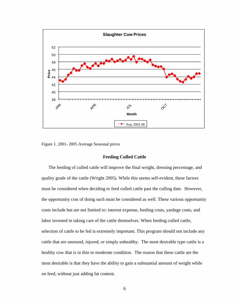
cattle going to the market at the same time, thus deflating prices (Figure 1).

Cull cow prices reach a seasonal minimum during the months of November,

December, and January. The seasonal price maximum for culled cattle occurs during the

months of March, April, and May. While most cows are culled in the fall due to a spring

calving season, there could be potential for profits returned to the producer by feeding the

culled cattle until the higher price prevails due to the changes in price seasonality (Feuz,

Stockton, and Bhattachary 2006). Research shows that lighter weight cattle suffer more

price seasonality than do heavier animals, except for cull cows, which have the largest

seasonal price swings of all cattle classes (Peel and Meyer 2001). Therefore, it can be

concluded that if we are able to provide an alternative time to market the cull cows versus

the normal time the culled cattle go to market, there may be a financial incentive

provided by the change in the price pattern. Therefore, any strategy that can market

culled cattle at any other time than when the majority of culled cattle are being marketed

could help increase revenue for the producer.

6

Figure 1. 2001- 2005 Average Seasonal prices

Feeding Culled Cattle

The feeding of culled cattle will improve the final weight, dressing percentage, and

quality grade of the cattle (Wright 2005). While this seems self-evident, these factors

must be considered when deciding to feed culled cattle past the culling date. However,

the opportunity cost of doing such must be considered as well. These various opportunity

costs include but are not limited to: interest expense, feeding costs, yardage costs, and

labor invested in taking care of the cattle themselves. When feeding culled cattle,

selection of cattle to be fed is extremely important. This program should not include any

cattle that are unsound, injured, or simply unhealthy. The most desirable type cattle is a

healthy cow that is in thin to moderate condition. The reason that these cattle are the

most desirable is that they have the ability to gain a substantial amount of weight while

on feed, without just adding fat content.

38

40

42

44

46

48

50

52P

rice

Month

Slaughter Cow Prices

Avg. 2001-05

7

The amount of time on feed and type of type are also something to consider. A

primary concern about time on feed is fat color. Some research has shown that fat color

will change from yellow to white in as few as 56 days, while other research has shown

that fat color will take as long as 105 days to change. The change in fat color represents a

financial reward to the producer (Wright 2005).

With that in mind, the choice of feeding program for culled cattle becomes very

important. The type of feeding program will affect the financial returns to keeping culled

cows past the culling date. There are numerous feeding scenarios for producers to choose

from but each will be dependent on the costs and expected returns from such a program.

A uniform feeding pattern for all culled cattle does not seem apparent with feed costs and

feeding options differing in various locations and feeding facilities (Wright 2005). A

decision tool that can aid a producer in knowing if a feeding program will return benefits

to the production program is estimating a partial budget. This budget should include

estimated feed costs, amount of time on feed, and other factors that are included in

production agriculture. By doing this, the producer is able to contrast different feeding

programs and decide which program nets the greatest returns to their enterprise (Feuz

2001).

Quality and Carcass Grades

Feuz (2001) reported that when feeding culled cattle, improving quality and

carcass grades are a main emphasis for the feeding program. By improving both of these

characteristics, the producer will receive an increased financial return for the cattle

marketed. The degree to which the USDA grade can be improved is a direct function of

the quality of feed program that the culled cattle are placed on. He also argues that a

8

feeding program with a higher quality of feed will return a higher USDA grade, but there

may not be a financial benefit to the producer if the costs of a higher quality feeding

program negate the increased revenue from the improved USDA grade.

When determining how to improve cattle slaughter grades, one must first consider

the cows’ present grade and to which grade they could improve. There are five distinct

grade classifications for slaughter cows, namely Commercial, Utility-Breaker, Utility-

Boner, Cutter, and Canner. Cull cow prices are dependent upon grade classification; and

the more desirable the grade, the higher the price. A producer may base his feeding

program around the current and expected grade of the cattle.

While culled cattle can gain large amounts of weight in relatively short amounts

of time on high grain diets, the higher gains do not come without cost. For instance,

calves and yearlings can normally achieve a pound of gain from 6 to 7 pounds of feed. In

contrast, to gain the same pound, culled cattle require 7.5 to 9.5 pounds of the same feed.

With the high average daily gains and relatively poor feed conversion rates, it would not

be unreasonable for a cow to consume dry matter at between 2.25% and 2.60 % of her

body weight (Wright 2005). This high level of intake will lead to high feed costs.

Therefore, any management factors that can be used to improve animal performance will

help improve the profitability of feeding cull cows

There has been some research done concerning the effects of feeding cull cows.

In Wright’s article, he used an experiment by Matulis et al. (1987) which showed that

feeding cull cows on a high energy diet for as few as 50 days can significantly increase

the final weight and improve the slaughter quality grade of the cattle. Carter and Johnson

9

(2006) show that cull cows on full feed from 28 to 56 days will increase their carcass

weight, due to an increase in carcass lean meat as well as carcass fat.

Factors Increasing Cull Cow Value

Despite the fact that 10% -25% of gross income for the producer comes from

culling cows; many producers focus their energy on marketing steers, but very few put

energy into marketing their cull cows (Hughes 1995). Making the decision to sell cull

cows at the time of culling versus feeding those cattle for an additional time before

marketing depends on three main factors, namely: 1) seasonality of cattle prices, 2) price

differences between cull cow slaughter grades and percentages of cull cows in each

grade, and 3) costs of feeding cull cows. While there are numerous strategies for

marketing culled cattle in Oklahoma, there are some considerations that a producer

should take into account when marketing cull cows (Feuz 2001).

Falconer, Bevers, and Bennett (2006) indicated that adding weight to thin cull

cows is particularly valuable, as compared to marketing crippled cattle directly to a

packer. Selling cull cows before they become fat, selling them outside of seasonal low

price periods, considering cull cows as a valuable asset , and always being cautious and

concerned about withdrawal times from antibiotics when marketing cows , would greatly

increase overall net returns. By using all these input factors and the amount of output

gained, the producer is able to use the information in a partial budget to make a

production decision (Peel and Doye 2007). This will help determine if feeding culled

cows is a profitable venture to the firm and if so, what type of feeding program they

should implement for optimal returns.

10

Effects of Canadian Cull Cow Market on U.S. Cull Cow Market

There are market forces that drastically impact the profitability of feeding culled

cattle. The single most drastic effect came from the U.S. government banning imports of

culled cattle from Canada after a cow in Canada was found with the disease BSE (Bovine

Spongiform Encephalopathy) (Feuz, Stockton, and Bhattachary 2006). This ban greatly

reduced the amount of cattle available for slaughter in the U.S, considering that 45% of

all cull cows in Canada were shipped to the U.S. for slaughter prior to the ban. This

caused an increase in slaughter prices for cattle in the U.S.

In general, a strong market and low cost of feeding, would suggest a greater

financial incentive to feeding cull cows because net returns are expected to be positive.

However, if the market turns weak and feeding costs are high, then there may not be as

much financial incentive to feeding culled cattle because net returns are expected to be

negative. The strength of the market is partially dependent on the trade restrictions or

lack thereof between the U.S. and Canada. In addition, the value of added absolute

weight gain is heavily dependent on magnitude of seasonal price change. Therefore,

adding value to cull cows when feeding costs are low and marketing prices are high is

better than selling cull cows when market prices are low and feeding costs are high.

Producers should keep a close eye on what policies are being discussed and what

decisions are being made in reference to the importing of cull cows from Canada when

considering feeding cull cows. Moreover, impact of dairy herd reductions should be taken

into consideration. If a producer does not pay attention to such information, he may

begin a feeding program that looks like it will return net profits only to see it return net

11

losses due to the changes in the market. So the effects of the Canadian cull cow market

have a direct relationship on producers’ production and marketing decisions.

In order to effectively estimate potential returns, producers should evaluate a

number of scenarios over several periods of time. For instance, the ban on Canadian beef

imports created a strong cull cow market here in the United States. However, with the

recent opening of the border, one may expect that the cull cow market may not remain as

strong.

Previous Studies on Feeding and Marketing Cull cows

To our knowledge, few studies have used the repeated measures technique to

estimate management production systems and timing strategies of cull cows.

Nevertheless, there are relevant studies on feeding and marketing cull cows. Thus,

William et al. (1980) used a stochastic dynamic programming model to estimate optimal

selling time and feeding levels prior to selling in Montana. Results from this study

showed that holding and feeding cull cows, assuming a single slaughter grade, would

increase expected net returns by $20 to $40 per head as compared to selling them at early

stages, November and December. However, due to a change in grade of cows being held

and fed, expected net returns would increase as much as $55 per head. Although this

study concluded that holding and feeding cows would be profitable, results would be

stronger if the feeding ration had been fully described to producers.

Garoian et al. (1990) used a dynamic programming model to determine optimal

strategies for marketing calves and yearlings from rangeland at a Texas Experiment

station ranch. Results from this study revealed that smaller cow herds and retaining

calves in the fall to sell as short or long yearlings could increase net returns over larger

12

traditional cow-calf production. Results also showed the marketing effect is always

positive while the feeding effect may be positive or negative depending on initial

conditions.

Schroeder and Featherstone (1990) used a discrete stochastic programming to

determine marketing and retention decisions for cow-calf producers. Hedges and options

were used to price at least a portion of the retained cattle for all but almost risk- neutral

producers. Results from this study indicated that more risk- adverse producers forward

priced almost all cows retained and the percentage of calves hedged relative to those

priced using options was highly sensitive to futures price volatility. Furthermore, results

revealed that under periods of high volatility, hedging was found to be the dominant

forward pricing strategy while under periods of low volatility, moderate risk-adverse

producers preferred to use options hedging. Finally, regardless of volatility level, strongly

risk-averse producers preferred hedging to put options.

Frasier and George (1994) used Markovian decision analysis to determine optimal

replacement and management policies for beef cows in a ranch in the Sandhills region of

Nebraska. Results from this study showed that during the optimal winter feeding

program, cows are maintained at a body condition slightly less than moderate with

immediate early return to estrus. This would result in earlier and shorter calving which

improves profitability. Providing cows with appropriate nutrition in the spring and winter

months and to cull cows that are not bred was found to be a better method of keeping a

shorter calving season.

13

CHAPTER III

METHODOLOGY

This chapter summarizes the methods and procedures used to determine

alternative production management systems and timing strategies for marketing cull

cows. Specifically, this section focuses on the conceptual framework, the data collection

methods, the experimental procedures, and the data analysis approach.

Conceptual framework

The goal of any cow-calf enterprise is to maximize profit, given a limited amount

of inputs such as labor, capital, land, and management. The timing of marketing cull

cows and the decision to hold and feed cull cows beyond culling, impacts the net revenue

of a cow-calf enterprise. However, the net return of keeping cull cows may increase or

decrease depending on the availability and affordability of forage and grain. The key

question is: Is it more profitable to sell cull cows immediately after they are culled or

should they be fed for alternative time periods and marketed later?

When considering a problem that deals with cull cows feeding and marketing

strategies, one may consider the following indirect profit function, where firms choose

sale dates and rations that maximize the net return.

14

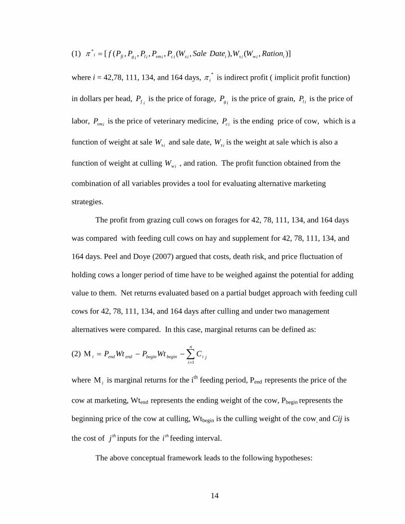
(1) )],(),,(,,,,([*iiwisiisicivmiligfii RationWWDateSaleWPPPPPf=π

where i = 42,78, 111, 134, and 164 days, *iπ is indirect profit ( implicit profit function)

in dollars per head, ifP is the price of forage,

igP is the price of grain, ilP is the price of

labor, ivmP is the price of veterinary medicine, icP is the ending price of cow, which is a

function of weight at sale isW and sale date, isW is the weight at sale which is also a

function of weight at culling iwW , and ration. The profit function obtained from the

combination of all variables provides a tool for evaluating alternative marketing

strategies.

The profit from grazing cull cows on forages for 42, 78, 111, 134, and 164 days

was compared with feeding cull cows on hay and supplement for 42, 78, 111, 134, and

164 days. Peel and Doye (2007) argued that costs, death risk, and price fluctuation of

holding cows a longer period of time have to be weighed against the potential for adding

value to them. Net returns evaluated based on a partial budget approach with feeding cull

cows for 42, 78, 111, 134, and 164 days after culling and under two management

alternatives were compared. In this case, marginal returns can be defined as:

(2)

∑=

−−=Μn

ijibeginbeginendendi CWtPWtP

1

where iΜ is marginal returns for the ith feeding period, Pend represents the price of the

cow at marketing, Wtend represents the ending weight of the cow, Pbegin represents the

beginning price of the cow at culling, Wtbegin is the culling weight of the cow, and Cij is

the cost of thj inputs for the thi feeding interval.

The above conceptual framework leads to the following hypotheses:

15

1. Due to higher grain costs relative to forage, it is hypothesized that cull cows fed

on grain would have lower net returns compared to cull cows grazing on grass.

2. Average daily gain, total gain, and cost per gain from grain fed cull cows are

higher than grass fed cull cows.

3. Factors such as beginning weight, average daily gain (ADG), feed cost per

gain, and treatment management systems significantly influence the net returns.

Methods, Procedures, and Data

An experiment involving feeding cull cows on grain and supplement versus cull

cows fed on forages was conducted by Samuel Roberts the Noble Foundation from

October 2007 to April 2008. This experiment was a two-factor experiment with repeated

measures comparing two levels of management alternatives (grass or dry lot) having n

cows randomly assigned to the two management alternatives and with measures taken

across 5 feeding intervals. Management alternative and length of feeding have fixed

effects, while individual cows have random effects on each response variable being

considered. Each management alternative includes 24 cows. Time periods included are

42, 78, 111, 134, and 164 days on feed. Thus, a mixed model that simultaneously

measures both fixed and random effects was chosen as most appropriate for this

experiment.

Data were collected approximately monthly on weight, USDA grade, dressing

percentage, costs (feed, animal health, etc.), and estimated market value. For each

interval, estimated animal performance and net returns were calculated. Both the

estimated USDA grade and estimated dressing percentage were used to assign a price to

each cow, based on prices reported by the Agricultural Marketing Service (AMS) for cull

16

cows in Oklahoma sold the same week. The value of each cow at each period was

calculated as follows cow weight (in hundred weights) multiplied by assigned line weight

prices. In addition, costs and value were estimated for each cow in each production

system at each feeding interval. Mean comparison between cows fed on grass and dry lot

at each weight period was analyzed.

Mean comparisons between grass fed cows and dry lot cows at each weigh period

were analyzed. A mixed model was estimated using a restricted maximum likelihood

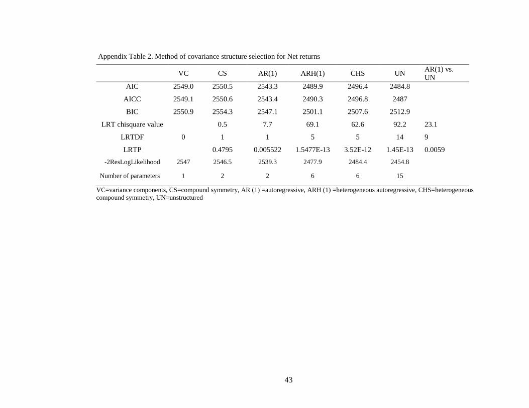
(REML) estimation technique. Likelihood ratio tests (LRT) indicated that an unstructured

covariance matrix was most appropriate in comparing mean and variance differences in

weight gain, ADG, cost per gain, and net margin between cull cows fed on grain and

supplement and those fed on forages (Appendix Page 47).

In order to test the hypotheses of this research, both maximum likelihood and

regression analysis were used.

Maximum likelihood estimation was used to implement the mixed model with

fixed and random effects in testing hypotheses 1 and 2, using the following statistical

equation:

The statistical model

(3) ijkY = µ + iα + kβ + ikαβ + )( ijθ + ijkε

where i is the dry lot or grass treatment, k is the feeding interval (42, 78, 111, 134, and

164 days), ijkY is the observation at time k on cows of treatment level i ( where ijkY

represents the value of various dependent variables to be compared), µ is the overall

mean, iα is the treatment level effect, kβ is the time effect, ikαβ is the treatment*time

17

interaction effect, )( ijθ is the random effect due to j cows in the thi treatment, and ijkε is

random error with ijkε ≈ iid N (0, 2εσ ).

Finally, the net returns obtained from the restricted maximum likelihood estimates

of both dry lot and grass treatment at 111 days were regressed on key variables such as

beginning weight, average daily gain (ADG), and feed cost per gain.

Regression analysis was used to test this hypothesis as follows:

Regression Model Specification

(4) Net returns = tFeedADGbegweight cos4321 ββββ +++ where net returns = net

returns, begweight= beginning weight, ADG= average daily gain, feedcost = feed cost

18

CHAPTER IV

RESULTS AND DISCUSSION

This section outlines results and discussions of the major findings. Specifically, this

chapter focuses on summary table and figures of some key physical and economic variables,

least square means comparison between grass and dry lot, and regression analysis.

Least Squares Means

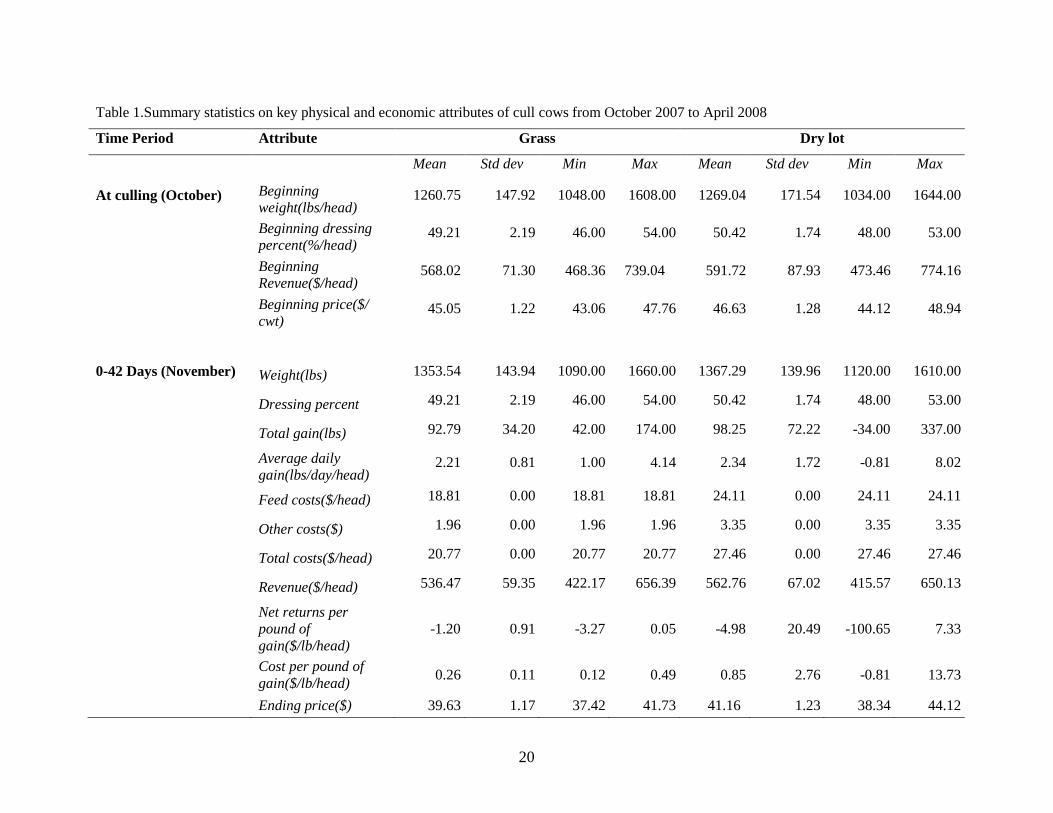
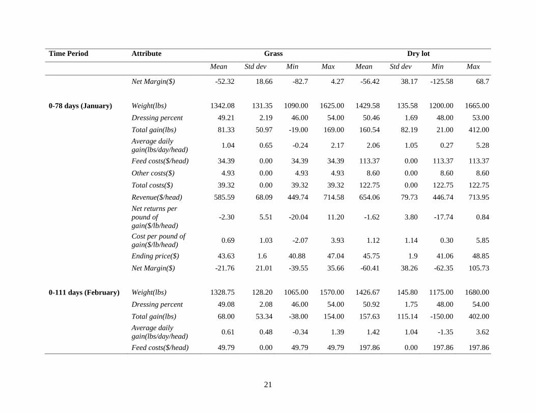
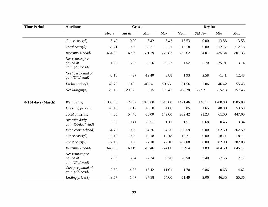
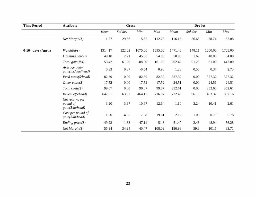
Table 1 reports summary statistics for some key variables considered in the study,

including , the mean, standard deviation, maximum and the minimum values of weight, average

daily gain, gain, revenue, feed cost, other cost, total cost, net returns, cost per gain, revenue per

gain, and dressing percentage.

Average means obtained from summary statistics were used to generate various graphs

to better understand the variation between dry lot and grass alternatives for these key variables.

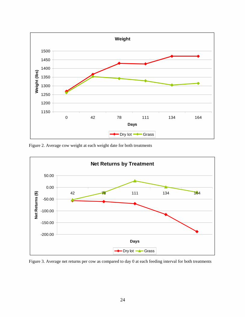
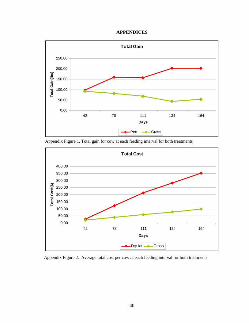
Figure 2 shows that weights for cows on dry lot for all intervals were higher than for cows on

grass. Also, Figure 3 shows that net returns for cows on grass were higher than for cows in dry

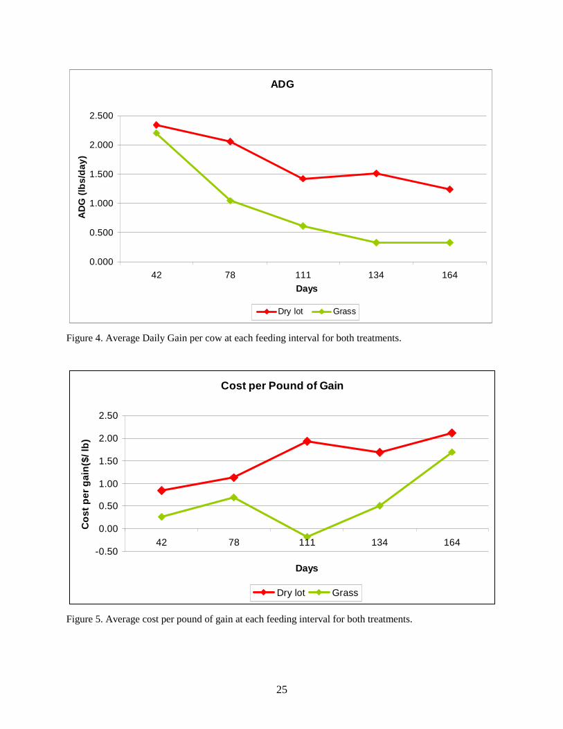
lot. Figure 4 shows that ADG for cows on dry lot were higher than for cows on grass. Moreover,

Figure 5 shows that cost per pound of gain of cows on dry lot were higher than for cows on

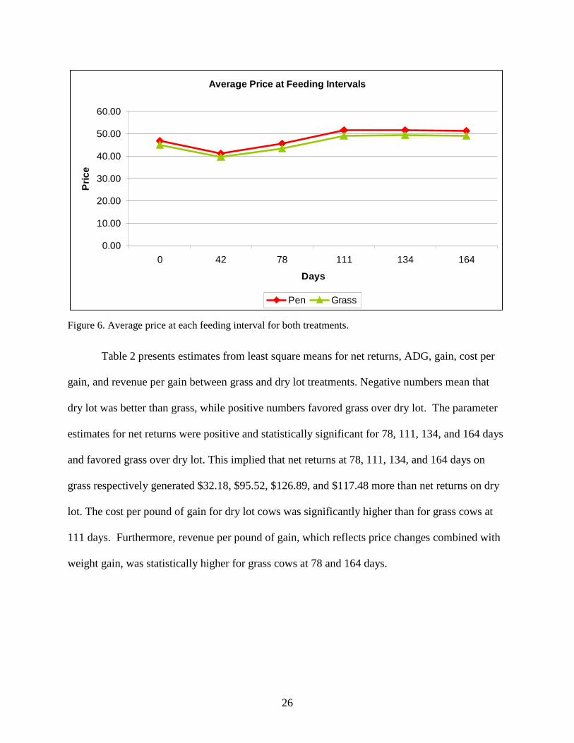
grass. Finally, Figure 6 shows how prices changed as result of the seasonal price patterns.

.

19

Figure 1 summarizes average of slaughter cow price from 2001 to 2005. Figure 1 showed

that prices were low in fall and high in spring.

Tables 1 and 2 in the appendix section were used to decide which covariance structures

best fit the repeated measures experiment. The results suggest that an unstructured covariance

structure was found to be the most appropriate for the model used in this study.

20

Table 1.Summary statistics on key physical and economic attributes of cull cows from October 2007 to April 2008

Time Period Attribute Grass Dry lot

Mean Std dev Min Max Mean Std dev Min Max

At culling (October) Beginning weight(lbs/head)

1260.75 147.92 1048.00 1608.00 1269.04 171.54 1034.00 1644.00

Beginning dressing percent(%/head)

49.21 2.19 46.00 54.00 50.42 1.74 48.00 53.00

Beginning Revenue($/head)

568.02 71.30 468.36 739.04 591.72 87.93 473.46 774.16

Beginning price($/ cwt)

45.05 1.22 43.06 47.76 46.63 1.28 44.12 48.94

0-42 Days (November) Weight(lbs) 1353.54 143.94 1090.00 1660.00 1367.29 139.96 1120.00 1610.00

Dressing percent 49.21 2.19 46.00 54.00 50.42 1.74 48.00 53.00

Total gain(lbs) 92.79 34.20 42.00 174.00 98.25 72.22 -34.00 337.00

Average daily gain(lbs/day/head)

2.21 0.81 1.00 4.14 2.34 1.72 -0.81 8.02

Feed costs($/head) 18.81 0.00 18.81 18.81 24.11 0.00 24.11 24.11

Other costs($) 1.96 0.00 1.96 1.96 3.35 0.00 3.35 3.35

Total costs($/head) 20.77 0.00 20.77 20.77 27.46 0.00 27.46 27.46

Revenue($/head) 536.47 59.35 422.17 656.39 562.76 67.02 415.57 650.13

Net returns per pound of gain($/lb/head)

-1.20 0.91 -3.27 0.05 -4.98 20.49 -100.65 7.33

Cost per pound of gain($/lb/head)

0.26 0.11 0.12 0.49 0.85 2.76 -0.81 13.73

Ending price($) 39.63 1.17 37.42 41.73 41.16 1.23 38.34 44.12

21



Net Margin($) -52.32 18.66 -82.7 4.27 -56.42 38.17 -125.58 68.7

0-78 days (January) Weight(lbs) 1342.08 131.35 1090.00 1625.00 1429.58 135.58 1200.00 1665.00


Total gain(lbs) 81.33 50.97 -19.00 169.00 160.54 82.19 21.00 412.00


1.04 0.65 -0.24 2.17 2.06 1.05 0.27 5.28

Feed costs($/head) 34.39 0.00 34.39 34.39 113.37 0.00 113.37 113.37

Other costs($) 4.93 0.00 4.93 4.93 8.60 0.00 8.60 8.60

Total costs($) 39.32 0.00 39.32 39.32 122.75 0.00 122.75 122.75

Revenue($/head) 585.59 68.09 449.74 714.58 654.06 79.73 446.74 713.95


-2.30 5.51 -20.04 11.20 -1.62 3.80 -17.74 0.84


0.69 1.03 -2.07 3.93 1.12 1.14 0.30 5.85

Ending price($) 43.63 1.6 40.88 47.04 45.75 1.9 41.06 48.85

Net Margin($) -21.76 21.01 -39.55 35.66 -60.41 38.26 -62.35 105.73

0-111 days (February) Weight(lbs) 1328.75 128.20 1065.00 1570.00 1426.67 145.80 1175.00 1680.00


Total gain(lbs) 68.00 53.34 -38.00 154.00 157.63 115.14 -150.00 402.00


0.61 0.48 -0.34 1.39 1.42 1.04 -1.35 3.62

Feed costs($/head) 49.79 0.00 49.79 49.79 197.86 0.00 197.86 197.86

22



Other costs($) 8.42 0.00 8.42 8.42 13.53 0.00 13.53 13.53

Total costs($) 58.21 0.00 58.21 58.21 212.18 0.00 212.17 212.18

Revenue($/head) 654.39 69.99 501.29 773.82 735.62 94.01 435.34 807.33


1.99 6.57 -5.16 29.72 -1.52 5.70 -25.01 3.74


-0.18 4.27 -19.40 3.88 1.93 2.58 -1.41 12.48

Ending price($) 49.25 1.46 46.14 53.65 51.56 2.06 46.42 55.43

Net Margin($) 28.16 29.87 6.15 109.47 -68.28 72.92 -152.3 157.45

0-134 days (March) Weight(lbs) 1305.00 124.07 1075.00 1540.00 1471.46 148.11 1200.00 1705.00


Total gain(lbs) 44.25 54.48 -68.00 149.00 202.42 91.23 61.00 447.00


0.33 0.41 -0.51 1.11 1.51 0.68 0.46 3.34

Feed costs($/head) 64.76 0.00 64.76 64.76 262.59 0.00 262.59 262.59

Other costs($) 13.18 0.00 13.18 13.18 18.71 0.00 18.71 18.71

Total costs($) 77.10 0.00 77.10 77.10 282.08 0.00 282.08 282.08

Revenue($/head) 646.89 69.19 513.46 774.00 729.4 91.89 464.59 845.17


2.86 3.34 -7.74 9.76 -0.50 2.40 -7.36 2.17


0.50 4.85 -15.42 11.01 1.70 0.86 0.63 4.62

Ending price($) 49.57 1.47 37.98 54.00 51.49 2.06 46.35 55.36

23



Net Margin($) 1.77 29.66 15.52 112.28 -116.13 56.68 -38.74 162.08

0-164 days (April) Weight(lbs) 1314.17 122.02 1075.00 1535.00 1471.46 148.11 1200.00 1705.00


Total gain(lbs) 53.42 61.20 -88.00 161.00 202.42 91.23 61.00 447.00


0.33 0.37 -0.54 0.98 1.23 0.56 0.37 2.73

Feed costs($/head) 82.39 0.00 82.39 82.39 327.32 0.00 327.32 327.32

Other costs($) 17.52 0.00 17.52 17.52 24.51 0.00 24.51 24.51

Total costs($) 99.07 0.00 99.07 99.07 352.61 0.00 352.60 352.61

Revenue($/head) 647.01 63.92 464.13 716.07 722.49 96.19 403.37 837.16


3.20 3.97 -10.67 12.64 -1.10 3.24 -10.41 2.61


1.70 4.85 -7.08 19.81 2.12 1.08 0.79 5.78

Ending price($) 49.23 1.33 47.14 51.8 51.47 2.46 48.94 56.28

Net Margin($) 55.34 34.94 -40.47 108.09 -186.98 59.3 -101.5 83.71

24

Weight

1150

1200

1250

1300

1350

1400

1450

1500

0 42 78 111 134 164

Days

Wei

gh

t (l

bs)

Dry lot Grass

Figure 2. Average cow weight at each weight date for both treatments

Net Returns by Treatment

-200.00

-150.00

-100.00

-50.00

0.00

50.00

42 78 111 134 164

Days

Net

Ret

urn

s ($

)

Dry lot Grass

Figure 3. Average net returns per cow as compared to day 0 at each feeding interval for both treatments

25

ADG

0.000

0.500

1.000

1.500

2.000

2.500

42 78 111 134 164

Days

AD

G (

lbs/

day

)

Dry lot Grass

Figure 4. Average Daily Gain per cow at each feeding interval for both treatments.

Cost per Pound of Gain

-0.50

0.00

0.50

1.00

1.50

2.00

2.50

42 78 111 134 164

Days

Co

st p

er g

ain

($/ l

b)

Dry lot Grass

Figure 5. Average cost per pound of gain at each feeding interval for both treatments.

26

Average Price at Feeding Intervals

0.00

10.00

20.00

30.00

40.00

50.00

60.00

0 42 78 111 134 164

Days

Pri

ce

Pen Grass

Figure 6. Average price at each feeding interval for both treatments.

Table 2 presents estimates from least square means for net returns, ADG, gain, cost per

gain, and revenue per gain between grass and dry lot treatments. Negative numbers mean that

dry lot was better than grass, while positive numbers favored grass over dry lot. The parameter

estimates for net returns were positive and statistically significant for 78, 111, 134, and 164 days

and favored grass over dry lot. This implied that net returns at 78, 111, 134, and 164 days on

grass respectively generated $32.18, $95.52, $126.89, and $117.48 more than net returns on dry

lot. The cost per pound of gain for dry lot cows was significantly higher than for grass cows at

111 days. Furthermore, revenue per pound of gain, which reflects price changes combined with

weight gain, was statistically higher for grass cows at 78 and 164 days.

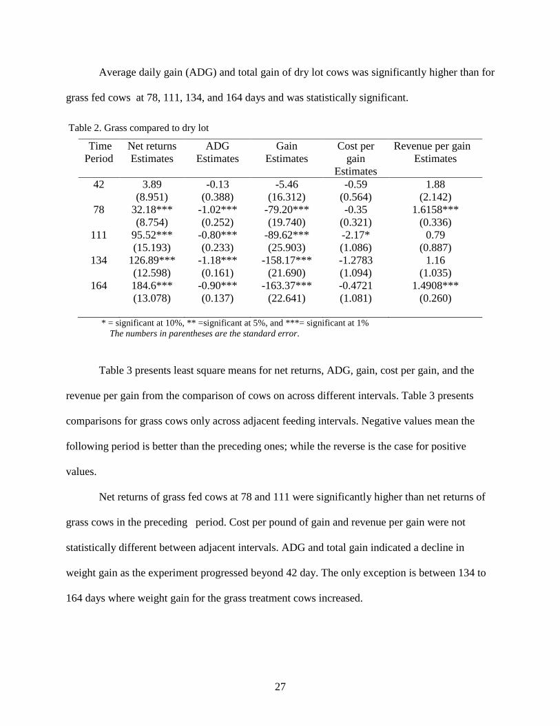
27

Average daily gain (ADG) and total gain of dry lot cows was significantly higher than for

grass fed cows at 78, 111, 134, and 164 days and was statistically significant.

Table 2. Grass compared to dry lot

Time Period

Net returns Estimates

ADG Estimates

Gain Estimates

Cost per gain

Estimates

Revenue per gain Estimates

42 3.89 (8.951)

-0.13 (0.388)

-5.46 (16.312)

-0.59 (0.564)

1.88 (2.142)

78 32.18*** (8.754)

-1.02*** (0.252)

-79.20*** (19.740)

-0.35 (0.321)

1.6158*** (0.336)

111 95.52*** (15.193)

-0.80*** (0.233)

-89.62*** (25.903)

-2.17* (1.086)

0.79 (0.887)

134 126.89*** (12.598)

-1.18*** (0.161)

-158.17*** (21.690)

-1.2783 (1.094)

1.16 (1.035)

164 184.6*** (13.078)

-0.90*** (0.137)

-163.37*** (22.641)

-0.4721 (1.081)

1.4908*** (0.260)

* = significant at 10%, ** =significant at 5%, and ***= significant at 1% The numbers in parentheses are the standard error.

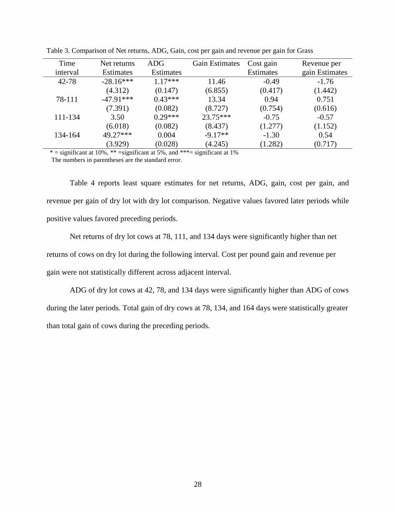
Table 3 presents least square means for net returns, ADG, gain, cost per gain, and the

revenue per gain from the comparison of cows on across different intervals. Table 3 presents

comparisons for grass cows only across adjacent feeding intervals. Negative values mean the

following period is better than the preceding ones; while the reverse is the case for positive

values.

Net returns of grass fed cows at 78 and 111 were significantly higher than net returns of

grass cows in the preceding period. Cost per pound of gain and revenue per gain were not

statistically different between adjacent intervals. ADG and total gain indicated a decline in

weight gain as the experiment progressed beyond 42 day. The only exception is between 134 to

164 days where weight gain for the grass treatment cows increased.

28

Table 3. Comparison of Net returns, ADG, Gain, cost per gain and revenue per gain for Grass

Time interval


ADG Estimates

Gain Estimates Cost gain Estimates


42-78 -28.16*** (4.312)

1.17*** (0.147)

11.46 (6.855)

-0.49 (0.417)

-1.76 (1.442)

78-111 -47.91*** (7.391)

0.43*** (0.082)

13.34 (8.727)

0.94 (0.754)

0.751 (0.616)

111-134 3.50 (6.018)

0.29*** (0.082)

23.75*** (8.437)

-0.75 (1.277)

-0.57 (1.152)

134-164 49.27*** (3.929)

0.004 (0.028)

-9.17** (4.245)

-1.30 (1.282)

0.54 (0.717)


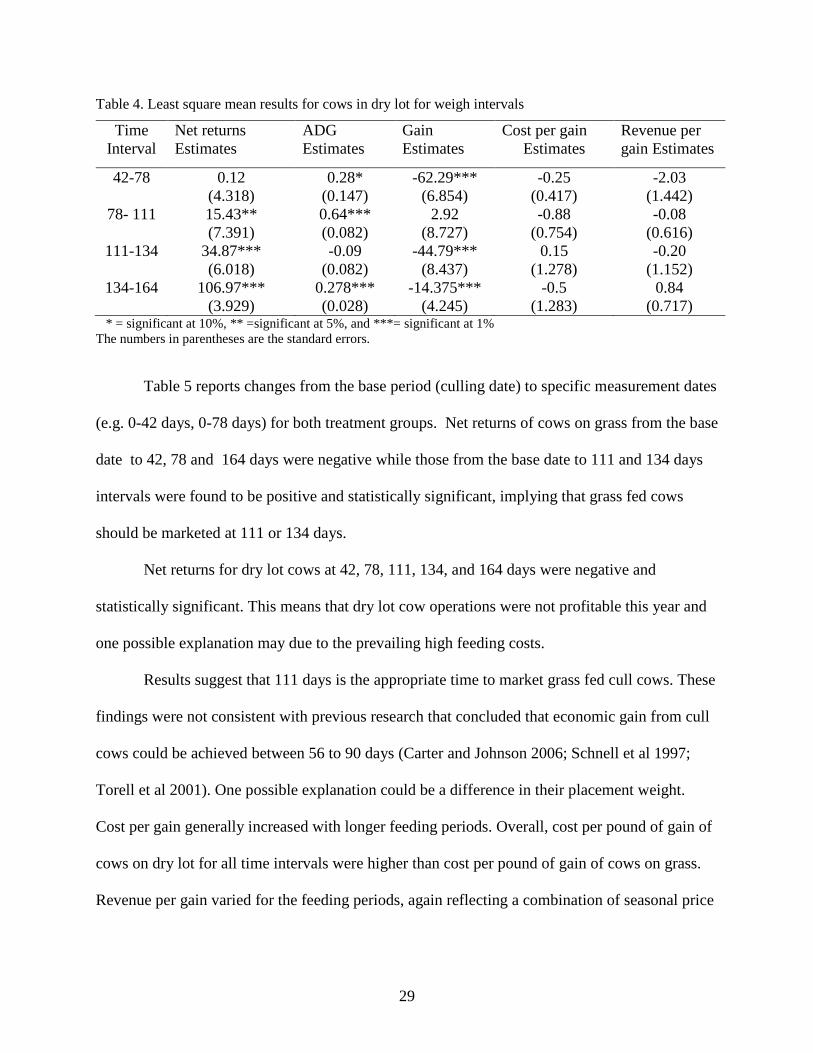
Table 4 reports least square estimates for net returns, ADG, gain, cost per gain, and

revenue per gain of dry lot with dry lot comparison. Negative values favored later periods while

positive values favored preceding periods.

Net returns of dry lot cows at 78, 111, and 134 days were significantly higher than net

returns of cows on dry lot during the following interval. Cost per pound gain and revenue per

gain were not statistically different across adjacent interval.

ADG of dry lot cows at 42, 78, and 134 days were significantly higher than ADG of cows

during the later periods. Total gain of dry cows at 78, 134, and 164 days were statistically greater

than total gain of cows during the preceding periods.

29

Table 4. Least square mean results for cows in dry lot for weigh intervals

Time Interval


ADG Estimates

Gain Estimates

Cost per gain Estimates


42-78 0.12 (4.318)

0.28* (0.147)

-62.29*** (6.854)

-0.25 (0.417)

-2.03 (1.442)

78- 111 15.43** (7.391)

0.64*** (0.082)

2.92 (8.727)

-0.88 (0.754)

-0.08 (0.616)

111-134 34.87*** (6.018)

-0.09 (0.082)

-44.79*** (8.437)

0.15 (1.278)

-0.20 (1.152)

134-164 106.97*** (3.929)

0.278*** (0.028)

-14.375*** (4.245)

-0.5 (1.283)

0.84 (0.717)

* = significant at 10%, ** =significant at 5%, and ***= significant at 1% The numbers in parentheses are the standard errors.

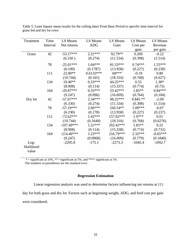
Table 5 reports changes from the base period (culling date) to specific measurement dates

(e.g. 0-42 days, 0-78 days) for both treatment groups. Net returns of cows on grass from the base

date to 42, 78 and 164 days were negative while those from the base date to 111 and 134 days

intervals were found to be positive and statistically significant, implying that grass fed cows

should be marketed at 111 or 134 days.

Net returns for dry lot cows at 42, 78, 111, 134, and 164 days were negative and

statistically significant. This means that dry lot cow operations were not profitable this year and

one possible explanation may due to the prevailing high feeding costs.

Results suggest that 111 days is the appropriate time to market grass fed cull cows. These

findings were not consistent with previous research that concluded that economic gain from cull

cows could be achieved between 56 to 90 days (Carter and Johnson 2006; Schnell et al 1997;

Torell et al 2001). One possible explanation could be a difference in their placement weight.

Cost per gain generally increased with longer feeding periods. Overall, cost per pound of gain of

cows on dry lot for all time intervals were higher than cost per pound of gain of cows on grass.

Revenue per gain varied for the feeding periods, again reflecting a combination of seasonal price

30

changes and weight changes for cows in both treatments. Overall, revenue per gain of cows on

grass for all time intervals was higher than revenue per gain for cows on dry lot.

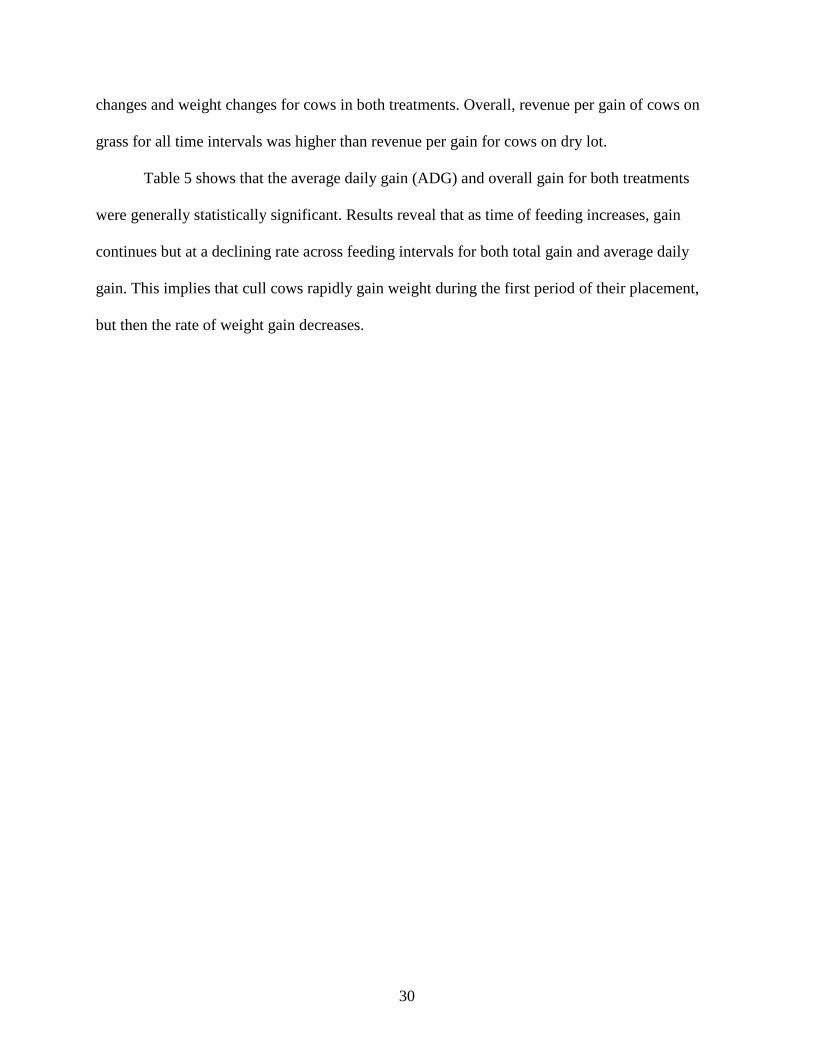
Table 5 shows that the average daily gain (ADG) and overall gain for both treatments

were generally statistically significant. Results reveal that as time of feeding increases, gain

continues but at a declining rate across feeding intervals for both total gain and average daily

gain. This implies that cull cows rapidly gain weight during the first period of their placement,

but then the rate of weight gain decreases.

31

Table 5. Least Square mean results for the culling dates From Base Period to specific time interval for grass fed and dry lot cows

Treatment Time

Interval LS Means Net returns

LS Means ADG

LS Means Gain

LS Means Cost per

gain

LS Means Revenue per gain

Grass 42 -53.17*** (6.330 )

2.21*** (0.274)

92.79** (11.534)

0.260 (0.398)

-0.22 (1.514)

78 -25.01*** (6.190)

1.04*** (0.1787)

81.33*** (13.958)

0.74*** (0.227)

1.55*** (0.238)

111 22.90** (10.744)

0.6133*** (0.165)

68*** (18.316)

-0.19 (0.768)

0.80 (0.627)

134 19.40** (8.908)

0.33*** (0.114)

44.25*** (15.337)

0.55 (0.774)

1.38* (0.73)

164 -29.87*** (9.247)

0.33*** (0.096)

53.42*** (16.009)

1.85** (0.764)

0.84*** (0.184)

Dry lot 42 -57.07*** (6.330)

2.34*** (0.274)

98.25*** (11.534)

0.845 ** (0.398)

-2.09 (1.514)

78 -57.19*** (6.190)

2.06*** (0.178)

160.54** (13.958)

1.09*** (0.227)

-0.07 (0.237)

111 -72.62*** (10.744)

1.42*** (0.1649)

157.62*** (18.316)

1.97** (0.768)

0.01 (0.6276)

134 -107.49*** (8.908)

1.51*** (0.114)

202.42*** (15.338)

1.83** (0.774)

0.22 (0.732)

164 -214.46*** (9.247)

1.23*** (0.0968)

216.79*** (16.009)

2.32*** (0.779)

-0.65*** (0.1840)

Log-likelihood

value

-2295.8

-175.1

-2273.3

-1045.4

-1092.7


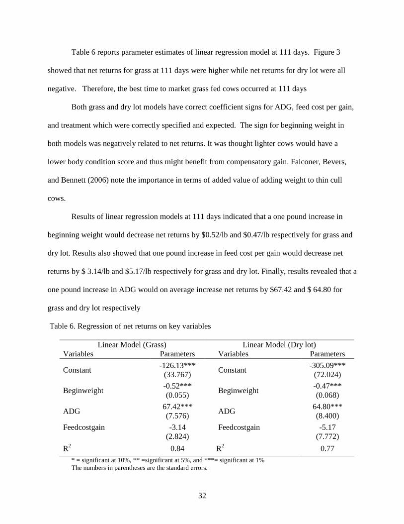
Regression Estimation

Linear regression analysis was used to determine factors influencing net returns at 111

day for both grass and dry lot. Factors such as beginning weight, ADG, and feed cost per gain

were considered.

32

Table 6 reports parameter estimates of linear regression model at 111 days. Figure 3

showed that net returns for grass at 111 days were higher while net returns for dry lot were all

negative. Therefore, the best time to market grass fed cows occurred at 111 days

Both grass and dry lot models have correct coefficient signs for ADG, feed cost per gain,

and treatment which were correctly specified and expected. The sign for beginning weight in

both models was negatively related to net returns. It was thought lighter cows would have a

lower body condition score and thus might benefit from compensatory gain. Falconer, Bevers,

and Bennett (2006) note the importance in terms of added value of adding weight to thin cull

cows.

Results of linear regression models at 111 days indicated that a one pound increase in

beginning weight would decrease net returns by $0.52/lb and $0.47/lb respectively for grass and

dry lot. Results also showed that one pound increase in feed cost per gain would decrease net

returns by $ 3.14/lb and $5.17/lb respectively for grass and dry lot. Finally, results revealed that a

one pound increase in ADG would on average increase net returns by $67.42 and $ 64.80 for

grass and dry lot respectively

Table 6. Regression of net returns on key variables

Linear Model (Grass) Linear Model (Dry lot) Variables Parameters Variables Parameters

Constant -126.13***

(33.767) Constant

-305.09*** (72.024)

Beginweight -0.52*** (0.055)

Beginweight -0.47*** (0.068)

ADG 67.42*** (7.576)

ADG 64.80*** (8.400)

Feedcostgain

-3.14 (2.824)

Feedcostgain

-5.17 (7.772)

R2 0.84 R2 0.77

* = significant at 10%, ** =significant at 5%, and ***= significant at 1% The numbers in parentheses are the standard errors.

33

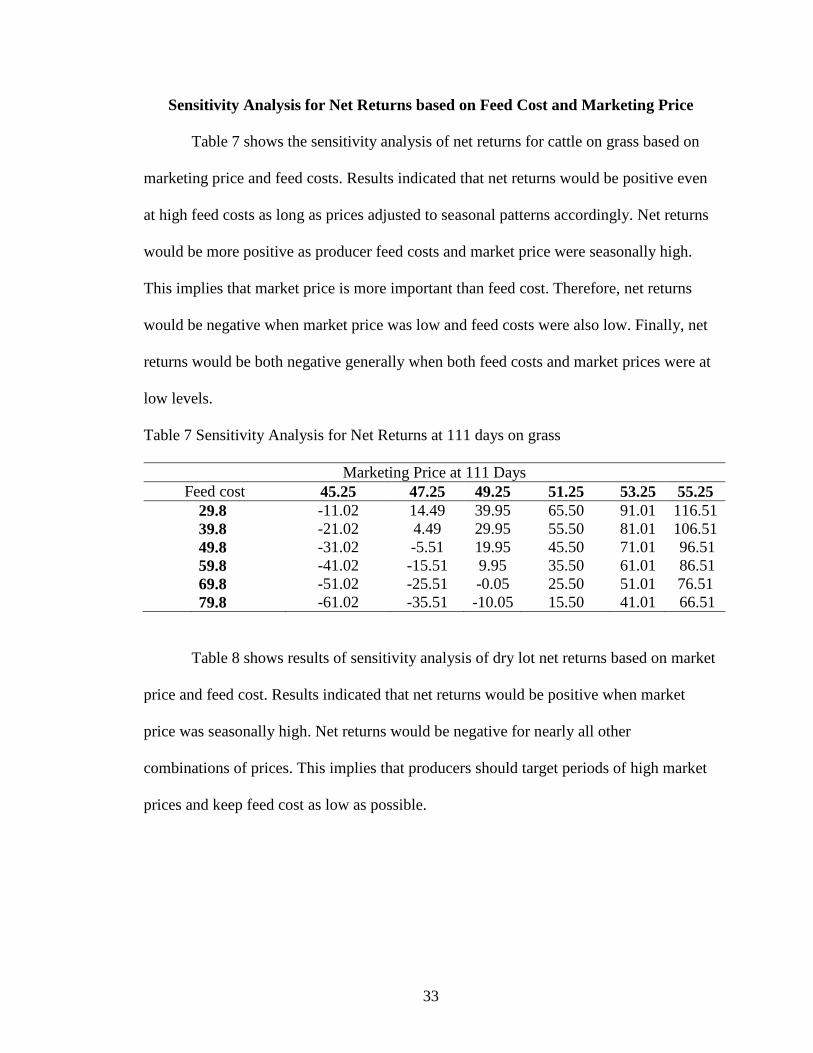
Sensitivity Analysis for Net Returns based on Feed Cost and Marketing Price

Table 7 shows the sensitivity analysis of net returns for cattle on grass based on

marketing price and feed costs. Results indicated that net returns would be positive even

at high feed costs as long as prices adjusted to seasonal patterns accordingly. Net returns

would be more positive as producer feed costs and market price were seasonally high.

This implies that market price is more important than feed cost. Therefore, net returns

would be negative when market price was low and feed costs were also low. Finally, net

returns would be both negative generally when both feed costs and market prices were at

low levels.

Table 7 Sensitivity Analysis for Net Returns at 111 days on grass

Marketing Price at 111 Days Feed cost 45.25 47.25 49.25 51.25 53.25 55.25

29.8 -11.02 14.49 39.95 65.50 91.01 116.51 39.8 -21.02 4.49 29.95 55.50 81.01 106.51 49.8 -31.02 -5.51 19.95 45.50 71.01 96.51 59.8 -41.02 -15.51 9.95 35.50 61.01 86.51 69.8 -51.02 -25.51 -0.05 25.50 51.01 76.51 79.8 -61.02 -35.51 -10.05 15.50 41.01 66.51

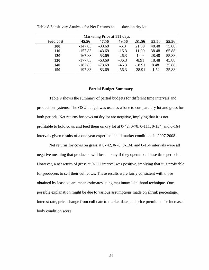
Table 8 shows results of sensitivity analysis of dry lot net returns based on market

price and feed cost. Results indicated that net returns would be positive when market

price was seasonally high. Net returns would be negative for nearly all other

combinations of prices. This implies that producers should target periods of high market

prices and keep feed cost as low as possible.

34

Table 8 Sensitivity Analysis for Net Returns at 111 days on dry lot

Marketing Price at 111 days Feed cost 45.56 47.56 49.56 .51.56 53.56 55.56

100 -147.83 -33.69 -6.3 21.09 48.48 75.88 110 -157.83 -43.69 -16.3 11.09 38.48 65.88 120 -167.83 -53.69 -26.3 1.09 28.48 55.88 130 -177.83 -63.69 -36.3 -8.91 18.48 45.88 140 -187.83 -73.69 -46.3 -18.91 8.48 35.88 150 -197.83 -83.69 -56.3 -28.91 -1.52 25.88

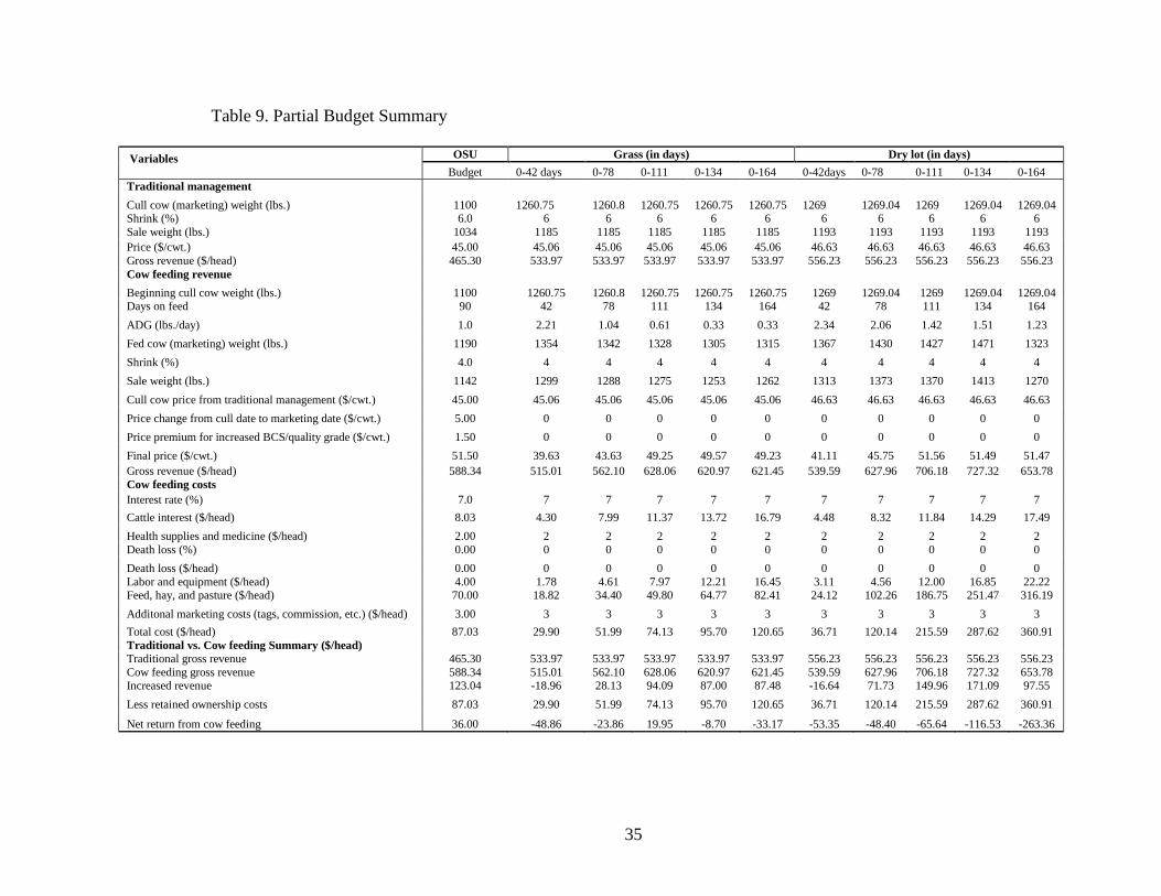
Partial Budget Summary

Table 9 shows the summary of partial budgets for different time intervals and

production systems. The OSU budget was used as a base to compare dry lot and grass for

both periods. Net returns for cows on dry lot are negative, implying that it is not

profitable to hold cows and feed them on dry lot at 0-42, 0-78, 0-111, 0-134, and 0-164

intervals given results of a one year experiment and market conditions in 2007-2008.

Net returns for cows on grass at 0- 42, 0-78, 0-134, and 0-164 intervals were all

negative meaning that producers will lose money if they operate on these time periods.

However, a net return of grass at 0-111 interval was positive, implying that it is profitable

for producers to sell their cull cows. These results were fairly consistent with those

obtained by least square mean estimates using maximum likelihood technique. One

possible explanation might be due to various assumptions made on shrink percentage,

interest rate, price change from cull date to market date, and price premiums for increased

body condition score.

35

Table 9. Partial Budget Summary

Variables

OSU Grass (in days) Dry lot (in days)

Budget 0-42 days 0-78 0-111 0-134 0-164 0-42days 0-78 0-111 0-134 0-164 Traditional management

Cull cow (marketing) weight (lbs.) 1100 1260.75 1260.8 1260.75 1260.75 1260.75 1269 1269.04 1269 1269.04 1269.04 Shrink (%) 6.0 6 6 6 6 6 6 6 6 6 6 Sale weight (lbs.) 1034 1185 1185 1185 1185 1185 1193 1193 1193 1193 1193 Price ($/cwt.) 45.00 45.06 45.06 45.06 45.06 45.06 46.63 46.63 46.63 46.63 46.63 Gross revenue ($/head) 465.30 533.97 533.97 533.97 533.97 533.97 556.23 556.23 556.23 556.23 556.23 Cow feeding revenue

Beginning cull cow weight (lbs.) 1100 1260.75 1260.8 1260.75 1260.75 1260.75 1269 1269.04 1269 1269.04 1269.04 Days on feed 90 42 78 111 134 164 42 78 111 134 164

ADG (lbs./day) 1.0 2.21 1.04 0.61 0.33 0.33 2.34 2.06 1.42 1.51 1.23

Fed cow (marketing) weight (lbs.) 1190 1354 1342 1328 1305 1315 1367 1430 1427 1471 1323

Shrink (%) 4.0 4 4 4 4 4 4 4 4 4 4

Sale weight (lbs.) 1142 1299 1288 1275 1253 1262 1313 1373 1370 1413 1270

Cull cow price from traditional management ($/cwt.) 45.00 45.06 45.06 45.06 45.06 45.06 46.63 46.63 46.63 46.63 46.63

Price change from cull date to marketing date ($/cwt.) 5.00 0 0 0 0 0 0 0 0 0 0

Price premium for increased BCS/quality grade ($/cwt.) 1.50 0 0 0 0 0 0 0 0 0 0

Final price ($/cwt.) 51.50 39.63 43.63 49.25 49.57 49.23 41.11 45.75 51.56 51.49 51.47 Gross revenue ($/head) 588.34 515.01 562.10 628.06 620.97 621.45 539.59 627.96 706.18 727.32 653.78 Cow feeding costs Interest rate (%) 7.0 7 7 7 7 7 7 7 7 7 7

Cattle interest ($/head) 8.03 4.30 7.99 11.37 13.72 16.79 4.48 8.32 11.84 14.29 17.49

Health supplies and medicine ($/head) 2.00 2 2 2 2 2 2 2 2 2 2 Death loss (%) 0.00 0 0 0 0 0 0 0 0 0 0

Death loss ($/head) 0.00 0 0 0 0 0 0 0 0 0 0 Labor and equipment ($/head) 4.00 1.78 4.61 7.97 12.21 16.45 3.11 4.56 12.00 16.85 22.22 Feed, hay, and pasture ($/head) 70.00 18.82 34.40 49.80 64.77 82.41 24.12 102.26 186.75 251.47 316.19

Additonal marketing costs (tags, commission, etc.) ($/head) 3.00 3 3 3 3 3 3 3 3 3 3

Total cost ($/head) 87.03 29.90 51.99 74.13 95.70 120.65 36.71 120.14 215.59 287.62 360.91 Traditional vs. Cow feeding Summary ($/head) Traditional gross revenue 465.30 533.97 533.97 533.97 533.97 533.97 556.23 556.23 556.23 556.23 556.23 Cow feeding gross revenue 588.34 515.01 562.10 628.06 620.97 621.45 539.59 627.96 706.18 727.32 653.78 Increased revenue 123.04 -18.96 28.13 94.09 87.00 87.48 -16.64 71.73 149.96 171.09 97.55

Less retained ownership costs 87.03 29.90 51.99 74.13 95.70 120.65 36.71 120.14 215.59 287.62 360.91

Net return from cow feeding 36.00 -48.86 -23.86 19.95 -8.70 -33.17 -53.35 -48.40 -65.64 -116.53 -263.36

36

CHAPTER V

CONCLUSIONS AND IMPLICATIONS

This study investigated whether cull cows should be sold immediately after being

culled from the herd or kept and fed on grass or in a dry lot for alternative periods of

time. An experiment involving 24 cull cows fed on grass and 24 cull cows fed in a dry lot

was conducted by the Samuel Roberts Noble Foundation from October 2007 to April

2008.

Results reveal that cows in both treatments gained a significant amount of weight

initially. Cows in the grass treatment then began losing weight on average while the dry

lot cows increased weight significantly. ADG for both groups declined following the

first 42 days. Cost of gain generally increased for both groups as the feeding period

increased. In general, cost per gain of cows in dry lot for all time intervals were higher

than cost per gain of cows on grass.

Prices increased over the experimental period generally in line with the seasonal

pattern. Therefore, increasing prices combined with modest weight gains led to higher

net returns at 78 days or more for both treatment groups. Net returns for grass-fed cows

exceeded those for dry lot cows for each period. Increasing cost per gain led to lower net

returns for the dry lot cows.

37

Regression results for net returns for both grass and dry lot at 111 days revealed that

beginning weight and feed cost per gain were negatively and significantly affected net

returns. Average daily gain was positively related to net returns for both models.

Results from sensitivity analysis of cows on grass suggested that net returns would be

positive when market price and feed were at high or when market price and feed cost

were respectively at high and low. This implied that market prices were dominant

regardless of feed cost level. However, the sensitivity analysis of dry lot revealed net

returns would be positive if only market price and feed cost were at high and low levels,

respectively.

In conclusion, holding cull cows beyond culling generated higher net returns than

selling them immediately after culling, for a grass feeding program after 111 days.

Producers should consider the weight, and condition of cows at culling, potential for

gain at reasonable cost, results at various potential end points, and the normal seasonal

pattern when considering how long to feed cows before marketing them. In sum,

producers should consider their own resources and the best use of those resources.

Limitations of this research include only one year of data, small sample size (48 cull

cows), and cows being in good body condition score. Further research comparing

profitability between bred cow and cull cow would be helpful to cow-calf producers.

38

REFERENCES

Carter, J. N., and Dwain D. Johnson.” Cull Cow Finishing Performance.” Unpublished Paper, Copy can be obtained from author, 2006.

Feuz, D. M. “Feeding and Marketing of Cull Cows. “ 2001. Retrieved October 24, 2007

Fromhttp://www.cabnr.unr.edu/AB/Extension/Cattleman/Cattleman2001/2001_005.PF

Feuz, D. M., Matt C .Stockton, and, Suparna. Bhattachary. “The Relationship of U.S.

and Canadian Cull Cow Price to Lean Beef Price: A DAG Analysis.” Paper selected for presentation at the American Agricultural Economics Association Annual Meeting July 2006.

Falconer, Larry, Stan Bevers, and Blake Bennett. “Marketing of Cull Cows.” 2006. Accessed on March 24, 2008 from http://mastermarketer.tamu.edu/tbrm/confprotoc/MCC.pdf

Frasier .W. M and George H. Pfeiffer.” Optimal Replacement and Management

Policies for Beef Cows.” American Journal of Agricultural Economic, Vol. 76-4(1994):847-858.

Garoian, L., J .W.Mjelde, and J.R. Conner. “Optimal Strategies for Marketing Calves and Yearlings from Rangeland.” American Journal of Agricultural Economics, 72- 3(1990):604-613.

Hughes, Harlan. “The Economics of Culling Cows.” 1995. Retrieved March 24, 2008 From http://www.beefmag.com/hughes/beef_economics_culling_cows/index.html

Jeffrey, C. N. and D. D. Johnson.” Cull Cow Finishing Performance. “Unpublished Paper, 2006. Copy can be obtained from author.

Little, R. D., A. Williams, R. Lacy, and Forrest, S. “Cull Cows Management and its Implications for Cow Calf Profitability.” Journal of Range Management, 55-2(2002):112-116.

Matulis, R. J., F. K. McKeith, D. B. Faulkner, L. L. Berger, and P. George. “Growth and carcass characteristics of cull cows after different times-on-feed.” J. Anim. Sci. 65(1987): 669-67

39

Peel, D. S. and D. Doye. “Cull Cows Grazing and Marketing Opportunities.” Unpublished paper 2007. Copy can be obtained from the author http://pods.dasnr.okstate.edu/docushare/dsweb/Get/Document-5148/AGEC-613web.pdf

Peel, Derrell and Steve Meyer. Cattle Price Seasonality. Managing for Today’s Cattle Market and beyond. 2002. Accessed on October 24, 2007 from http://agecon.uwyo.edu/RiskMgt/marketrisk/cattlepriceseasonality2002.pdf

Pritchard, R. H., and P. T. Berg. 1993.” Feedlot performance and carcass traits of culled cows fed for slaughter.” South Dakota Beef Report CATTLE 93-20:101-107.

Schnell, T.D., K.E. Belk, J.D. Miller, and R.K. Smith, G.C. “Performance, Carcass, and

Palatability Days.” http://jas.fass.org/cgi/content/abstract/75/5/1195 Accessed on March 24, 2008.

Schroeder T. C and Allen. M. Featherstone. “Dynamic Marketing and Retention Decisions for Cow-Calf Producers.” American Journal of Agricultural Economics 72-4(1990):1028-1040.

Troxel.R.T. “Managing and Marketing Cull Cows.” University of Arkansas Cooperative

Extension Service 2001http://www.uaex.edu/Other_Areas/publications/PDF/FSA-3058.pdf Accessed on February 14, 2008.

Torell, Ron. Willie Riggs, Cevin Jones, and Ken Conley.”Marketing Alternatives of Cull Cows: A Case study.” 2001. Unpublished paper. Copy available from author. https://www.ag.unr.edu/ab/Extension/Cattleman/Cattleman2001/2001_006.PDF

Wright. C. L. “Managing and Marketing Cull Cows.” 2005. Retrieved March 24, 2008

from http://beef.unl.edu/beefreports/symp-2005-20-XIX.pdf Yager .W. A., Clyde Greer .R. and Oscar. R. Burt. “Optimal Policies for Marketing

Cull Beef Cows.” American Journal of Agricultural Economics 62-3(1980):1456-467

http://www.ams.usda.gov/AMSv1.0/ams.fetchTemplateData.do? TemplateA&avID=MarketNewsAndTransportationData&leftNav=MarketNewsAndTransportationData&page=MarketNewsAndTransportationData&acct=AMSPW

40

Total Gain

0.00

50.00

100.00

150.00

200.00

250.00

42 78 111 134 164

Days

To

tal

Gai

n(l

bs)

Pen Grass

APPENDICES

Appendix Figure 1. Total gain for cow at each feeding interval for both treatments

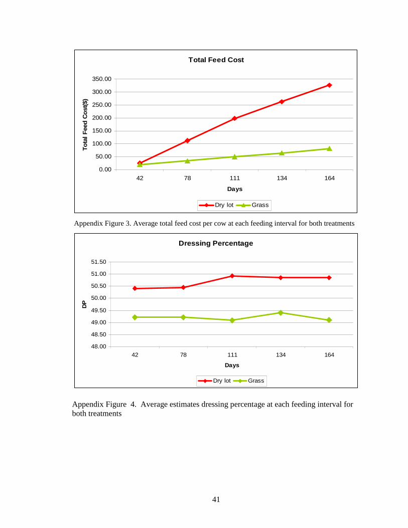
Total Cost

0.00

50.00

100.00

150.00

200.00

250.00

300.00

350.00

400.00

42 78 111 134 164

Days

To

tal

Co

st($

)

Dry lot Grass

Appendix Figure 2. Average total cost per cow at each feeding interval for both treatments

41

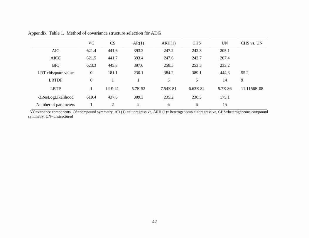
Total Feed Cost

0.00

50.00

100.00

150.00

200.00

250.00

300.00

350.00

42 78 111 134 164

Days

To

tal

Fee

d C

ost

($)

Dry lot Grass

Appendix Figure 3. Average total feed cost per cow at each feeding interval for both treatments

Dressing Percentage

48.00

48.50

49.00

49.50

50.00

50.50

51.00

51.50

42 78 111 134 164

Days

DP

Dry lot Grass

Appendix Figure 4. Average estimates dressing percentage at each feeding interval for both treatments

42

Appendix Table 1. Method of covariance structure selection for ADG

VC CS AR(1) ARH(1) CHS UN CHS vs. UN

AIC 621.4 441.6 393.3 247.2 242.3 205.1

AICC 621.5 441.7 393.4 247.6 242.7 207.4

BIC 623.3 445.3 397.6 258.5 253.5 233.2

LRT chisquare value 0 181.1 230.1 384.2 389.1 444.3 55.2

LRTDF 0 1 1 5 5 14 9

LRTP 1 1.9E-41 5.7E-52 7.54E-81 6.63E-82 5.7E-86 11.1156E-08

-2ResLogLikelihood 619.4 437.6 389.3 235.2 230.3 175.1

Number of parameters 1 2 2 6 6 15

VC=variance components, CS=compound symmetry, AR (1) =autoregressive, ARH (1)= heterogeneous autoregressive, CHS=heterogeneous compound symmetry, UN=unstructured

43

Appendix Table 2. Method of covariance structure selection for Net returns

VC CS AR(1) ARH(1) CHS UN AR(1) vs. UN

AIC 2549.0 2550.5 2543.3 2489.9 2496.4 2484.8

AICC 2549.1 2550.6 2543.4 2490.3 2496.8 2487

BIC 2550.9 2554.3 2547.1 2501.1 2507.6 2512.9

LRT chisquare value 0.5 7.7 69.1 62.6 92.2 23.1

LRTDF 0 1 1 5 5 14 9

LRTP 0.4795 0.005522 1.5477E-13 3.52E-12 1.45E-13 0.0059

-2ResLogLikelihood 2547 2546.5 2539.3 2477.9 2484.4 2454.8

Number of parameters 1 2 2 6 6 15

VC=variance components, CS=compound symmetry, AR (1) =autoregressive, ARH (1) =heterogeneous autoregressive, CHS=heterogeneous compound symmetry, UN=unstructured

VITA

ZAKOU AMADOU

Candidate for the Degree of

Master of Science Thesis: MANAGEMENT PRODUCTION SYSTEMS AND TIMING STRATEGIES

FOR CULL COWS Major Field: Agricultural Economics Biographical:

Personal Data: Born in Bouki (Loga), Dosso State, Niger in January 01, 1976, the son of Amadou Issaka and Aissa Beido.

Education: Graduated from Usmanu Danfodiyo University, Sokoto State, Nigeria, in 2002; received a Bachelor of Agriculture degree in Agricultural Economics and Extension; completed the requirements for the Master of Science in Agricultural Economics at Oklahoma State University, Stillwater, Oklahoma May 2009.

Experience: Staff at the Ministry of Livestock Resources in Niger from January 2003 to January 2006

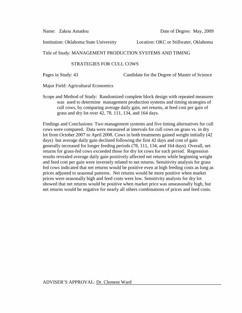
Name: Zakou Amadou Date of Degree: May, 2009 Institution: Oklahoma State University Location: OKC or Stillwater, Oklahoma Title of Study: MANAGEMENT PRODUCTION SYSTEMS AND TIMING

STRATEGIES FOR CULL COWS Pages in Study: 43 Candidate for the Degree of Master of Science

Major Field: Agricultural Economics Scope and Method of Study: Randomized complete block design with repeated measures

was used to determine management production systems and timing strategies of cull cows, by comparing average daily gain, net returns, at feed cost per gain of grass and dry lot over 42, 78, 111, 134, and 164 days.

Findings and Conclusions: Two management systems and five timing alternatives for cull cows were compared. Data were measured at intervals for cull cows on grass vs. in dry lot from October 2007 to April 2008. Cows in both treatments gained weight initially (42 days) but average daily gain declined following the first 42 days and cost of gain generally increased for longer feeding periods (78, 111, 134, and 164 days). Overall, net returns for grass-fed cows exceeded those for dry lot cows for each period. Regression results revealed average daily gain positively affected net returns while beginning weight and feed cost per gain were inversely related to net returns. Sensitivity analysis for grass fed cows indicated that net returns would be positive even at high feeding costs as long as prices adjusted to seasonal patterns. Net returns would be more positive when market prices were seasonally high and feed costs were low. Sensitivity analysis for dry lot showed that net returns would be positive when market price was unseasonally high, but net returns would be negative for nearly all others combinations of prices and feed costs. ADVISER’S APPROVAL: Dr. Clement Ward

Documents

MANAGEMENT PRODUCTION SYSTEMS AND TIMING …digital.library.okstate.edu/etd/Amadou_okstate_0664M_10264.pdf · 1. 2001-2005 Average seasonal ... calf producers traditionally cull and