Arabian Journal for Science and Engineeringhttps://doi.org/10.1007/s13369-019-03749-2

RESEARCH ART ICLE - PETROLEUM ENGINEER ING

Reserve Estimation Using Decline Curve Analysis forBoundary-Dominated Flow Dry Gas Wells

Emeka Emmanuel Okoro1 · Austin Okoh2 · Evelyn Bose Ekeinde2 · Adewale Dosunmu2

Received: 3 October 2017 / Accepted: 2 February 2019© King Fahd University of Petroleum &Minerals 2019

AbstractDiverse techniques have been developed to improve the estimated reserves for boundary-dominated flow dry gas wells.The various methods developed and published in various journals on how to estimate reserves range from material balancetechniques to decline curve analysis. Among the various techniques, decline curves are found quite accurate in predictinggood gas performance in the absence of well-known reservoir parameters. There are basically two issues that practically arisein applying decline curve analysis, particularly in boundary-dominated flow dry gas wells. First, it has been noted that it isdifficult to match a decline exponent, especially at an early stage of well depletion, even with worthy quality data. Secondly,decline exponent is not constant from observation, but changes with declining production. So, the study has provided a newmethod based on numerical curve fitting to accurately match the Arps’ decline curve function, even at the early depletionstage, and account for the changing decline exponent. Once the match objective is satisfied, future predictions can be madewith a reasonable degree of assurance. Finally, the study showed that for the Arps’ decline equation to be valid, the declineexponent must be between 0 and 1.

Keywords Decline curve analysis · Dry gas well · Boundary-dominated flow · Numerical curve fitting

1 Introduction

As part of the gas reservoir development plan, the utmostimperative requirements are the estimation of reserves andprediction of gas sources or reservoirs of the entire or certainfields. Various techniques have been developed lately to tryto improve estimation of reserves [1]. Usually, most infor-mation about the history of production is available to startanalyses on reservoir reserves using decline curve analysis[2,3].

The different methods developed and published in a vari-ety of journals for the evaluation of reserves range frommaterial balance approach to decline curve techniques anal-ysis. Among the techniques, gas well performance canaccurately be forecasted using decline curve techniques inabsence of some reservoir parameters. It seems to be a

B Emeka Emmanuel Okoroemeka.okoro@covenantuniversity.edu.ng

1 School of Petroleum Engineering, Covenant University, Ota,Nigeria

2 Petroleum Engineering Department, University of PortHarcourt, Port Harcourt, Nigeria

vital method for making future forecasts and assessing theoriginal gas in place and hydrocarbons reserves [4]. Theseestimates are necessary for volumetric reservoirs in deter-mining if a particular project is economically and financiallyviable [5,6]. According to Ling and He [7], Arps explainsthat the decline curve analysis is a prediction method whichextrapolates the production trends. They presented empiricalconditions and relationships to evaluate rate behaviour overtime.

In the early 1980s, Fetkovich introduced an analysis ofdecline curve using type curves. This, in fact, is a graphicalmethod for visual matching or comparison of observationaldata using pre-plotted curves on a log–log diagram [8]. Thetype curve was applied to both transient flow period andboundary-dominated flow period. The type-curve analysiswas designed for rapid performance evaluation when wellswere produced under a constant bottom-hole pressure andcould be used to predict future performance forecast.

In 1985, Carter introduced a type curve which featuredFetkovich’s type specially designed for gas reservoirs. Thetechnique was based on numerical solution of gas depletionin finite reservoir for radial symmetrical linear flow settingsat constant bottom-hole pressures [7]. Carter introduced a

123

Arabian Journal for Science and Engineering

lambda sign that reflects the size of the pressure reduction/drawdown. Cater type curvewas not as direct and all-purposewhen compared with how Fetkovich provides understandingand implicit guidance for analysing reservoir data.Carter alsointroduced other type curves that could handle the changesoften associated with gas properties corresponding to pres-sure [9].

A few years later, Fraim and Wattenbarger in Chapra andCanale [10] studied gas wells and recognized a standardpseudo-time function to force the data from the reservoirgas to match the liquid solution for a stable well-flow pres-sure introduced by Fetkovich. However, this calculationinvolves iteration which is time-consuming [11]. Palacioand Blasingame [12] raised the question of variable non-constant wellbore pressure in boundary-dominated flow gaswells [13].

1.1 Current Challenges

This study is informed by the several unaddressed limita-tions in reserve estimation from decline curve analysis ofboundary-dominated flow wells and multilayered gas well.One of the limitations among others is:

1. The difficulty of finding a proper nonlinear algorithmto tune the Arp’s decline equation to match historicalgas production. For this reason, most applications optfor type-curvematchingwhose inefficiency to adequatelypredict tight gas behaviour has been widely criticized.

The current practice in the industry provides the user withthree types of decline curves to choose the one to fit. Thequestion is, “how does the user know arbitrarily the typeof decline depletion the reservoir is undergoing?” Further,it must be understood that the curvature of a decline couldchange during production. Accordingly, the study not beingoblivious that the exponential and harmonic declines are lim-iting subsets of the hyperbolic decline opt to rigorously fit thehyperbolic decline. If the decline exponents are zero or veryclose to zero, then the decline is exponential. The decline isharmonic if the decline exponent is 1 or reasonably close to1. This allows the depletion history tune itself adaptively tothe most suitable decline curvature.

In the view of Poston and Poe [14], “decline curve analy-sis is probably the most widely used and least understoodproduction forecasting technique currently in use in theindustry. Analysis of decline curves provides an unsophis-ticated reservoir evaluation tool, but profound economicdecisions often rest on the outcome of the prediction”. Thereason is not farfetched. The basic concept behind declinecurve analysis is nonlinear curve fitting. And the mathe-matics of nonlinear curve fitting has generated all kindsof reconciled conflict as to the technique of evaluating the

parameters of the nonlinear function. This study thereforeresolves this conflict bydescribing an automatic self-adaptivecomputer nonlinear regression algorithm. It is based on non-linear multi-parameter iteration method that discovers theminimum of a function that is expressed as the sum of thesquares of the nonlinear real-valued function.

This study provides a new method to accurately matchthe Arp’s decline curve function, even at the early depletionstage.Once thematch objective is satisfied, future predictionscan be made with a reasonable degree of assurance.

2 Empirical Review

2.1 Decline Curve Analysis

Declining production is caused by changes in bottom-holepressure, productivity index, the efficiency of vertical, andhorizontal fluid lift equipment, among others [15]. Decliningproduction with respect to decreasing rate is expressed by:

D = − 1

q

dq

dt= −d ln q

dt(1)

where

q = flow rate

D = rate of nominal decline

Cutler argues that most of the decline curves usually encoun-tered are hyperbolic, and the values of b vary from 0 to0.7. Arps reduced the maximum value of this interval to0.4. Lefkovit and Mathews found that for some conditionsof gravity drainage b = 0.5. Fetkovich (1973) proved thatthe analysis of the hyperbolic decline curve has a theoreticalbasis. It also uses hyperbolic decline as a diagnostic methodto show that the fall index ranges from 0 to 0.5 for gas reser-voirs and 0.3333 to 0.6667 for reservoirs driven by gas.

There are two ways of predicting the decline exponent:the Arp decline curve analysis and the type-curve declinecurve analysis. The Arp’s method varies decline exponentand decline rate in the Arp’s equation to achieve a matchbetween production history and theArp’s equation. This typeof history matching is daunting because the Arp’s equationis an ill-posed nonlinear equation.

2.2 Arp’s Decline Curve Analysis

In 1945, Arps working with Eq. 2 anticipated that the cur-vature in the rate-time decline curve can be articulatedmathematically with the hyperbolic equation defined below

q = qi(1 + bDi t)1/b

(2)

123

Arabian Journal for Science and Engineering

qi is the initial flow rate.Though the hyperbolic decline is most common, yet the

exponential and harmonic declines are applied in practicedue to their simplicity.

It is the intent of this study to effectively match the pasttrend with the Arp’s equation. Against this limitation, caremust be taken to ensure that the technique is not improp-erly applied, as has been observed in different literatures.To remark, the conditions to ensure that the past productiontrends remain unchanged for the application of decline curveanalysis are: the late time, constant bottom-hole pressure,and at or near capacity conditions. The late-time conditiondefines the pseudo-steady-state condition in which the wellis in a boundary-dominated condition; that is, the well isdraining a constant drainage area.

2.3 Type-Curve Decline Analysis

This analysis is based on the fact that a graph of log�Pversus log t has the same shape as the graph of log PD versuslog tD , but are parallel to the defined or given shift on the twoaxes.

Fetkovich projected that the dimensionless-variablesapproach can be stretched for use in decline curve analysisto streamline the calculations [8]. The variables for declinecurve dimensionless flow rate, qDd = q/qi was introducedand decline curve dimensionless time, tDd = Di t . Arps’relationships, during the steady-state or semi-steady-stateflowing periods.

In furtherance, Fetkovich imposed the transient constantterminal pressure solution to the dimensionless form of thediffusivity equation and presented the dimensionless declinerate at different dimensionless rD = re/rwa and the dimen-sionless decline time thus:

qDd = qikh(Pi−P)

141.2Bμ[ln rD− 1

2

]= qD

[ln rD − 1

2

](3)

Fetkovich arrived at his unified type curve by combining thetransient analytical solution and the empirical pseudo-steady-state solution.

Compilation of the late-time data gives an indication of thereserves, which are a direct function of the drainage radiusre. Knowing the coincidence of the drainage radius and thetransient data match, we can calculate the effective radius ofthe well using the re/rw parameter, and from there we canobtain the skin factor S using rwa = rwe−S .

Initially, Fetkovich developed type curves for gas and oilwells producing at constant pressure. Carter [16] published anew set of type curves developed for specialized analysis ofgas well data [17]. Carter noted that the pressure change dueto the fluid properties and nature have a great influence in pre-

dicting the gas reservoir productivity and performance. Thisinnovation is a change in the gas viscosity–compressibilityproduct μgcg, which Fetkovich neglected. Carter recognizedyet another set of decline curves for a boundary-dominatedflow that practises a new correlating parameter λ to charac-terize the changes inμgcg during depletion. The λ parameter,called the dimensionless drawdown correlating parameter, isselected to reflect themeasure of pressure drawdown onμgcgand represented as follows:

λ =(μgcg

)i(

μgcg)avg

=(μgcg

)i

2

[m (Pi ) − m (Pwf)

PiZi

− PwfZwf

](4)

For λ = 1, it shows a negligible drawdown effect and cor-responds to the b = 0 on the Fetkovich exponential declinecurve. Values of λ are the range between 0.55 and 1.0.

Fetkovich type curve does not take into account varia-tions of bottom-hole flowing pressure for a transient regime;this limitation is considered only on cases of boundary-dominatedflowand it is accounted for empirically.Moreover,for the gas wells, varying PVT properties and the reser-voir pressure were not considered. In 1993, Palacio andBlasingame developed a novel method for changing produc-tion data from gas wells, bottom-hole flowing pressure, andvariable rates into equivalent constant rate liquid data thatcan allow liquid solutions to be applied when modelling agas flow.

Thismethod applies a formofmaterial balance timewhichrequires only the harmonic decline for matching type curve.

3 Model Development

3.1 Methodology

Gas Decline Exponent Estimation before Decline Curve Anal-ysis

This study performs its analysis by numerically fitting theArps’ decline function to obtained gas decline exponent,decline rate, and initial gas flow rate from which initial gasin place is estimated. Being that a numerical approach isdesired, an estimate of decline exponent is required to ini-tialize the tuning algorithm. The values of decline exponentand decline rate lie between 0 and 1. So, it would not be outof place to initialize decline exponent and decline rate as 0.5.But such initialization may lead the algorithm to converge tothe nearest local minimum, which may not be the requiredminimum. To illustrate, suppose for the production trend, theArps’ decline curve has local minima at decline exponentsof 0.6 and 0.8, then an initial guess of 0.5 will converge thealgorithm to 0.6 in lieu of 0.8.

123

Arabian Journal for Science and Engineering

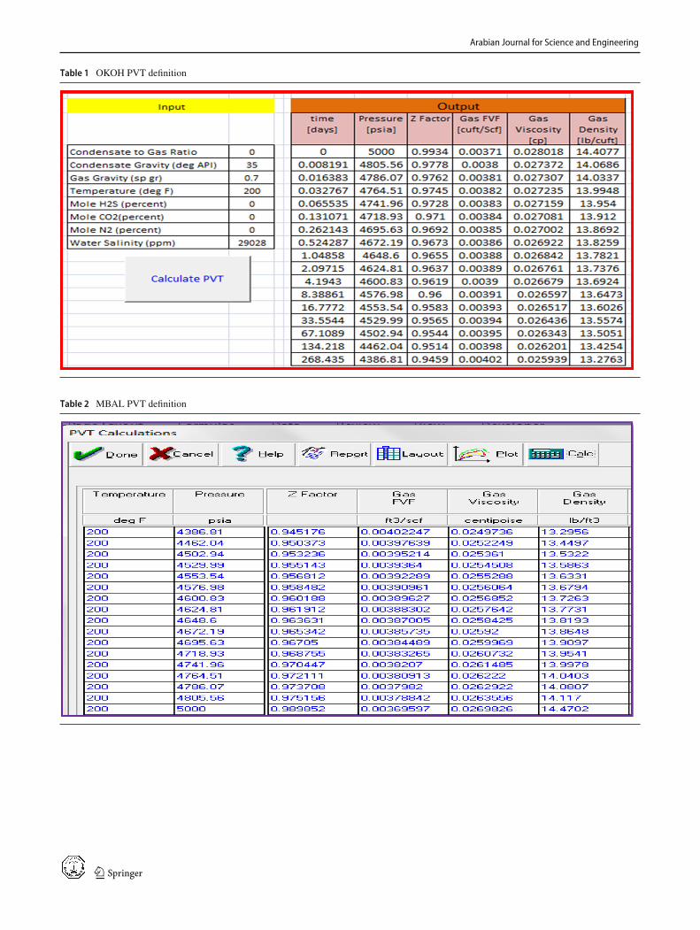
Table 1 OKOH PVT definition

Table 2 MBAL PVT definition

123

Arabian Journal for Science and Engineering

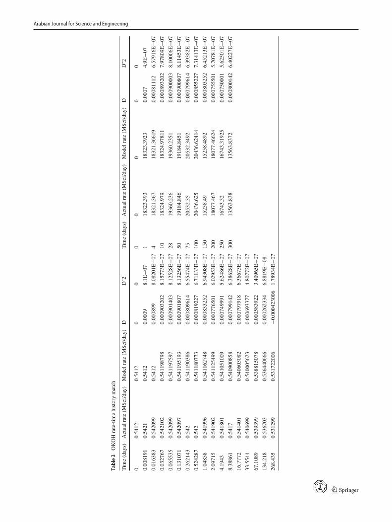
Table3

OKOHrate-tim

ehistorymatch

Tim

e(days)

Actualrate(M

Scf/day)

Modelrate(M

Scf/day)

DDˆ2

Tim

e(days)

Actualrate(M

Scf/day)

Modelrate(M

Scf/day)

DDˆ2

00.5412

0.5412

00

00

00

0

0.008191

0.5421

0.5412

0.0009

8.1E

−07

118323.393

18323.3923

0.0007

4.9E

−07

0.016383

0.542099

0.5412

0.000899

8.08201E

−07

418321.367

18321.36619

0.00081112

6.57916E

−07

0.032767

0.542102

0.541198798

0.000903202

8.15773E

−07

1018324.979

18324.97811

0.000893202

7.97809E

−07

0.065535

0.542099

0.541197597

0.000901403

8.12528E

−07

2819360.236

19360.2351

0.000900003

8.10006E

−07

0.131071

0.542097

0.541195193

0.000901807

8.13256E

−07

5019184.846

19184.8451

0.000900807

8.11453E

−07

0.262143

0.542

0.541190386

0.000809614

6.55474E

−07

7520532.35

20532.3492

0.000799614

6.39382E

−07

0.524287

0.542

0.541180773

0.000819227

6.71133E

−07

100

20436.625

20436.62414

0.000855227

7.31413E

−07

1.04858

0.541996

0.541162748

0.000833252

6.94308E

−07

150

15258.49

15258.4892

0.000803252

6.45213E

−07

2.09715

0.541902

0.541125499

0.000776501

6.02953E

−07

200

18077.467

18077.46624

0.000755501

5.70781E

−07

4.1943

0.541801

0.541051009

0.000749991

5.62486E

−07

250

16743.32

16743.31925

0.000750001

5.62501E

−07

8.38861

0.5417

0.540900858

0.000799142

6.38628E

−07

300

13563.838

13563.8372

0.000800142

6.40227E

−07

16.7772

0.541401

0.540603082

0.000797918

6.36673E

−07

33.5544

0.540699

0.540005623

0.000693377

4.80772E

−07

67.1089

0.539399

0.538815078

0.000583922

3.40965E

−07

134.218

0.536703

0.536440666

0.000262334

6.8819E−0

8

268.435

0.531299

0.531722006

−0.000423006

1.78934E

−07

123

Arabian Journal for Science and Engineering

0.53

0.535

0.54

0.545

0 50 100 150 200 250

Rate

[M

MSc

f/da

y]

Time [days]

Actual Rate

Model Rate

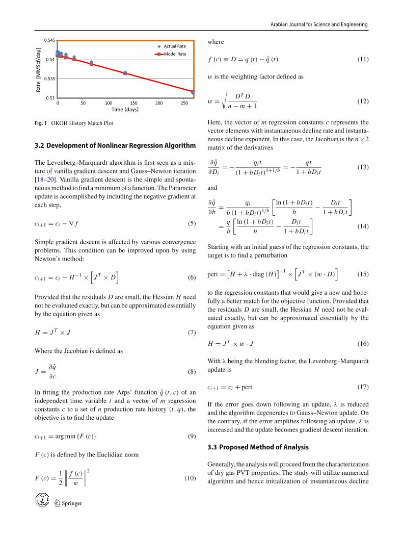
Fig. 1 OKOH History Match Plot

3.2 Development of Nonlinear Regression Algorithm

The Levenberg–Marquardt algorithm is first seen as a mix-ture of vanilla gradient descent and Gauss–Newton iteration[18–20]. Vanilla gradient descent is the simple and sponta-neousmethod tofind aminimumof a function. TheParameterupdate is accomplished by including the negative gradient ateach step,

ci+1 = ci − ∇ f (5)

Simple gradient descent is affected by various convergenceproblems. This condition can be improved upon by usingNewton’s method:

ci+1 = ci − H−1 ×[J T × D

](6)

Provided that the residuals D are small, the Hessian H neednot be evaluated exactly, but can be approximated essentiallyby the equation given as

H = J T × J (7)

Where the Jacobian is defined as

J = ∂q̂

∂c(8)

In fitting the production rate Arps’ function q̂ (t, c) of anindependent time variable t and a vector of m regressionconstants c to a set of n production rate history (t, q), theobjective is to find the update

ci+1 = argmin {F (c)} (9)

F (c) is defined by the Euclidian norm

F (c) = 1

2

∥∥∥∥f (c)

w

∥∥∥∥2

(10)

where

f (c) ≡ D = q (t) − q̂ (t) (11)

w is the weighting factor defined as

w =√

DT D

n − m + 1(12)

Here, the vector of m regression constants c represents thevector elements with instantaneous decline rate and instanta-neous decline exponent. In this case, the Jacobian is the n×2matrix of the derivatives

∂ q̂

∂Di= − qi t

(1 + bDi t)1+1/b = − qt

1 + bDi t(13)

and

∂ q̂

∂b= qi

b (1 + bDi t)1/b

[ln (1 + bDi t)

b− Di t

1 + bDi t

]

= q

b

[ln (1 + bDi t)

b− Di t

1 + bDi t

](14)

Starting with an initial guess of the regression constants, thetarget is to find a perturbation

pert = [H + λ · diag (H)

]−1 ×[J T × (w · D)

](15)

to the regression constants that would give a new and hope-fully a better match for the objective function. Provided thatthe residuals D are small, the Hessian H need not be eval-uated exactly, but can be approximated essentially by theequation given as

H = J T × w · J (16)

With λ being the blending factor, the Levenberg–Marquardtupdate is

ci+1 = ci + pert (17)

If the error goes down following an update, λ is reducedand the algorithm degenerates to Gauss–Newton update. Onthe contrary, if the error amplifies following an update, λ isincreased and the update becomes gradient descent iteration.

3.3 ProposedMethod of Analysis

Generally, the analysiswill proceed from the characterizationof dry gas PVT properties. The study will utilize numericalalgorithm and hence initialization of instantaneous decline

123

Arabian Journal for Science and Engineering

Table 4 Comparison of excelsolver software & OKOHMODEL

Time (days) Actual rate(MMSCFD)

Excel solvermodel rate(MMSCFD)

OKOHmodel rate(MMSCFD)

% Deviationbetween excelSolver soft-ware & Studymodel

0 0.5412 0.5412 0.5412 0

0.008191 0.5421 0.541199708 0.5412 −5.39542E−05

0.016383 0.542099 0.541199416 0.5412 −0.000107908

0.032767 0.542102 0.541198831 0.541198798 6.09757E−06

0.065535 0.542099 0.541197662 0.541197597 1.20104E−05

0.131071 0.542097 0.541195325 0.541195193 2.43905E-05

0.262143 0.542 0.541190649 0.541190386 4.85966E−05

0.524287 0.542 0.541181299 0.541181975 −0.000124912

1.04858 0.541996 0.541162599 0.541162748 −2.75333E−05

2.09715 0.541902 0.541125203 0.541125499 −5.47008E-05

4.1943 0.541801 0.541050423 0.54105221 −0.000330283

8.38861 0.5417 0.540900917 0.54090326 −0.000433166

16.7772 0.541401 0.54060212 0.540607883 −0.001066034

33.5544 0.540699 0.540005375 0.540015216 −0.001822389

67.1089 0.539399 0.538815279 0.538834221 −0.003515491

134.218 0.536703 0.536448583 0.536478784 −0.005629803

268.435 0.531299 0.53176856 0.531797573 −0.005455945

rate and instantaneous decline exponent follow. The instan-taneous decline exponent is given by

bE = 1

2

[1 − pwf

pi

](18)

The initialization of instantaneous decline exponent dependson the reservoir flowing pressure and initial reservoir pres-sure. The Arps’ decline function is regressed to obtainthe values of instantaneous decline rate and instantaneousdecline exponent that will provide a match of the regressionmodel and the actual rate decline. The objective of the tuningprocess is to find a Levenberg–Marquadrt perturbation thatwould update the initial estimate of Di and b

ci+1 = ci + pert (19)

Here, ci+1 is an updated column vector of Di and b improvedfrom their initialized state to obtain a match.

With the values of instantaneous decline rate and instanta-neous decline exponent determined, cumulative gas produc-tion is evaluated from the following equation:

Gp =∫ t

0q̂dt (20)

The gas initially in place is computed by extrapolating P/Zplot to cut the cumulative production axis. This value is

Table 5 Cumulative gas and reserve estimate

Time (days) Gp (MMScf) P/Z (Psia) Reserve (MMScf)

0 0 5033.1712 6407.69231

0.008191 0.004432967 4914.7278 6407.68787

0.016383 0.00886647 4902.5212 6407.68344

0.032767 0.017733462 4888.945 6407.67457

0.065535 0.035467389 4874.6624 6407.65684

0.131071 0.070935012 4859.9876 6407.62137

0.262143 0.14186934 4845.0491 6407.55044

0.524287 0.28373432 4829.927 6407.40857

1.04858 0.567452278 4814.6122 6407.12486

2.09715 1.134820719 4799.0692 6406.55749

4.1943 2.26932779 4783.3013 6405.42298

8.38861 4.537406843 4767.5174 6403.1549

16.7772 9.06978988 4751.9055 6398.62252

33.5544 18.11955636 4736.1202 6389.57275

67.1089 36.15930069 4717.8638 6371.53301

134.218 72.00105593 4690.0029 6335.69125

268.435 142.7452933 4637.9344 6264.94701

checked by estimating the gas in place from the geometryof the reservoir:

GI I P = π(r2e − r2w

)hθ/Bgi (21)

123

Arabian Journal for Science and Engineering

4600

4650

4700

4750

4800

4850

4900

4950

5000

5050

5100

0 50 100 150 200

P/Z

[Psi

a]

Cumula�ve Gas Produced [MMScf]

P/Z Plot

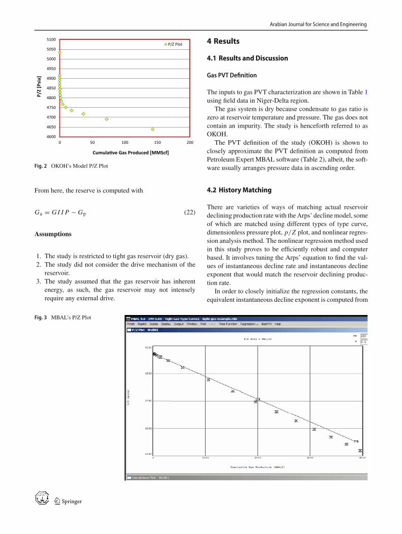
Fig. 2 OKOH’s Model P/Z Plot

From here, the reserve is computed with

Ga = GI I P − Gp (22)

Assumptions

1. The study is restricted to tight gas reservoir (dry gas).2. The study did not consider the drive mechanism of the

reservoir.3. The study assumed that the gas reservoir has inherent

energy, as such, the gas reservoir may not intenselyrequire any external drive.

4 Results

4.1 Results and Discussion

Gas PVT Definition

The inputs to gas PVT characterization are shown in Table 1using field data in Niger-Delta region.

The gas system is dry because condensate to gas ratio iszero at reservoir temperature and pressure. The gas does notcontain an impurity. The study is henceforth referred to asOKOH.

The PVT definition of the study (OKOH) is shown toclosely approximate the PVT definition as computed fromPetroleum Expert MBAL software (Table 2), albeit, the soft-ware usually arranges pressure data in ascending order.

4.2 History Matching

There are varieties of ways of matching actual reservoirdeclining production ratewith theArps’ declinemodel, someof which are matched using different types of type curve,dimensionless pressure plot, p/Z plot, and nonlinear regres-sion analysis method. The nonlinear regression method usedin this study proves to be efficiently robust and computerbased. It involves tuning the Arps’ equation to find the val-ues of instantaneous decline rate and instantaneous declineexponent that would match the reservoir declining produc-tion rate.

In order to closely initialize the regression constants, theequivalent instantaneous decline exponent is computed from

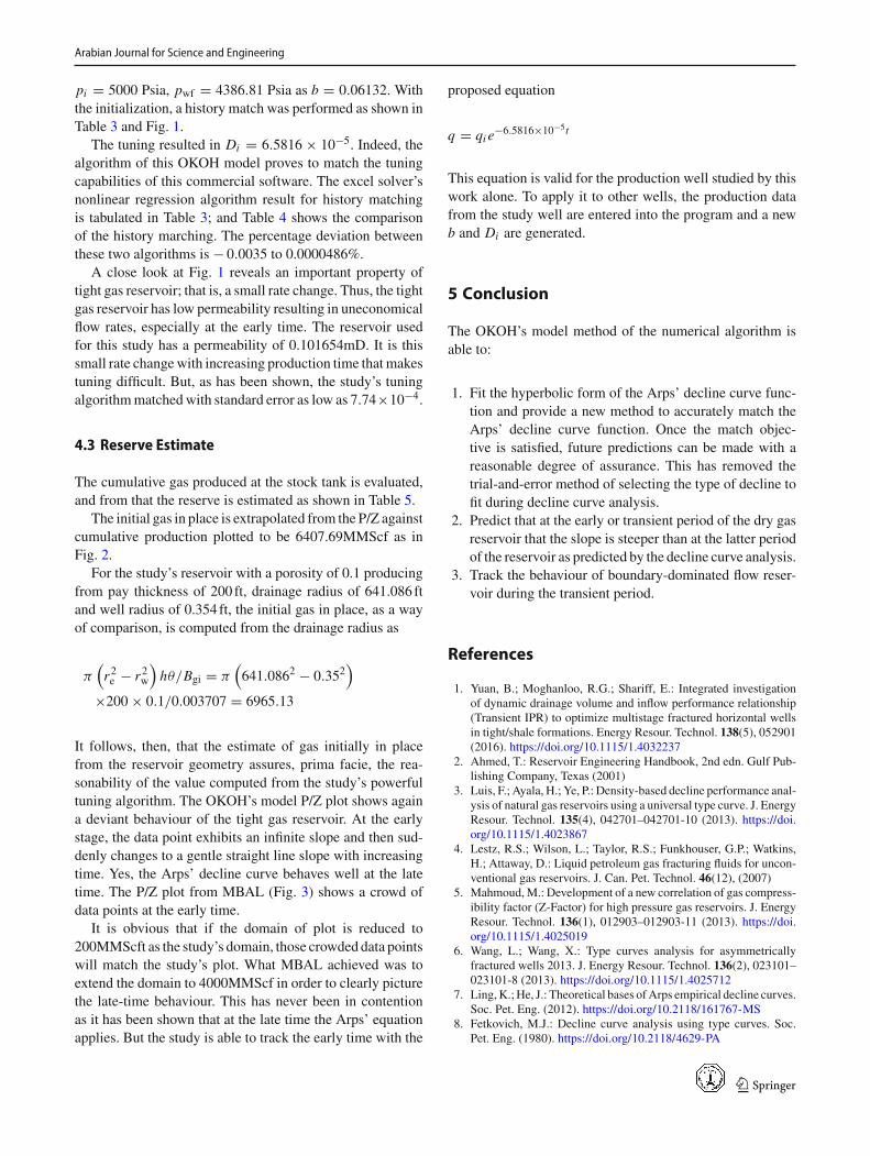
Fig. 3 MBAL’s P/Z Plot

123

Arabian Journal for Science and Engineering

pi = 5000 Psia, pwf = 4386.81 Psia as b = 0.06132. Withthe initialization, a history match was performed as shown inTable 3 and Fig. 1.

The tuning resulted in Di = 6.5816 × 10−5. Indeed, thealgorithm of this OKOH model proves to match the tuningcapabilities of this commercial software. The excel solver’snonlinear regression algorithm result for history matchingis tabulated in Table 3; and Table 4 shows the comparisonof the history marching. The percentage deviation betweenthese two algorithms is − 0.0035 to 0.0000486%.

A close look at Fig. 1 reveals an important property oftight gas reservoir; that is, a small rate change. Thus, the tightgas reservoir has low permeability resulting in uneconomicalflow rates, especially at the early time. The reservoir usedfor this study has a permeability of 0.101654mD. It is thissmall rate changewith increasing production time that makestuning difficult. But, as has been shown, the study’s tuningalgorithmmatchedwith standard error as low as 7.74×10−4.

4.3 Reserve Estimate

The cumulative gas produced at the stock tank is evaluated,and from that the reserve is estimated as shown in Table 5.

The initial gas in place is extrapolated from the P/Z againstcumulative production plotted to be 6407.69MMScf as inFig. 2.

For the study’s reservoir with a porosity of 0.1 producingfrom pay thickness of 200 ft, drainage radius of 641.086 ftand well radius of 0.354 ft, the initial gas in place, as a wayof comparison, is computed from the drainage radius as

π(r2e − r2w

)hθ/Bgi = π

(641.0862 − 0.352

)

×200 × 0.1/0.003707 = 6965.13

It follows, then, that the estimate of gas initially in placefrom the reservoir geometry assures, prima facie, the rea-sonability of the value computed from the study’s powerfultuning algorithm. The OKOH’s model P/Z plot shows againa deviant behaviour of the tight gas reservoir. At the earlystage, the data point exhibits an infinite slope and then sud-denly changes to a gentle straight line slope with increasingtime. Yes, the Arps’ decline curve behaves well at the latetime. The P/Z plot from MBAL (Fig. 3) shows a crowd ofdata points at the early time.

It is obvious that if the domain of plot is reduced to200MMScft as the study’s domain, those crowded data pointswill match the study’s plot. What MBAL achieved was toextend the domain to 4000MMScf in order to clearly picturethe late-time behaviour. This has never been in contentionas it has been shown that at the late time the Arps’ equationapplies. But the study is able to track the early time with the

proposed equation

q = qi e−6.5816×10−5t

This equation is valid for the production well studied by thiswork alone. To apply it to other wells, the production datafrom the study well are entered into the program and a newb and Di are generated.

5 Conclusion

The OKOH’s model method of the numerical algorithm isable to:

1. Fit the hyperbolic form of the Arps’ decline curve func-tion and provide a new method to accurately match theArps’ decline curve function. Once the match objec-tive is satisfied, future predictions can be made with areasonable degree of assurance. This has removed thetrial-and-error method of selecting the type of decline tofit during decline curve analysis.

2. Predict that at the early or transient period of the dry gasreservoir that the slope is steeper than at the latter periodof the reservoir as predicted by the decline curve analysis.

3. Track the behaviour of boundary-dominated flow reser-voir during the transient period.

References

1. Yuan, B.; Moghanloo, R.G.; Shariff, E.: Integrated investigationof dynamic drainage volume and inflow performance relationship(Transient IPR) to optimize multistage fractured horizontal wellsin tight/shale formations. Energy Resour. Technol. 138(5), 052901(2016). https://doi.org/10.1115/1.4032237

2. Ahmed, T.: Reservoir Engineering Handbook, 2nd edn. Gulf Pub-lishing Company, Texas (2001)

3. Luis, F.; Ayala, H.; Ye, P.: Density-based decline performance anal-ysis of natural gas reservoirs using a universal type curve. J. EnergyResour. Technol. 135(4), 042701–042701-10 (2013). https://doi.org/10.1115/1.4023867

4. Lestz, R.S.; Wilson, L.; Taylor, R.S.; Funkhouser, G.P.; Watkins,H.; Attaway, D.: Liquid petroleum gas fracturing fluids for uncon-ventional gas reservoirs. J. Can. Pet. Technol. 46(12), (2007)

5. Mahmoud,M.: Development of a new correlation of gas compress-ibility factor (Z-Factor) for high pressure gas reservoirs. J. EnergyResour. Technol. 136(1), 012903–012903-11 (2013). https://doi.org/10.1115/1.4025019

6. Wang, L.; Wang, X.: Type curves analysis for asymmetricallyfractured wells 2013. J. Energy Resour. Technol. 136(2), 023101–023101-8 (2013). https://doi.org/10.1115/1.4025712

7. Ling,K.;He, J.: Theoretical bases ofArps empirical decline curves.Soc. Pet. Eng. (2012). https://doi.org/10.2118/161767-MS

8. Fetkovich, M.J.: Decline curve analysis using type curves. Soc.Pet. Eng. (1980). https://doi.org/10.2118/4629-PA

123

Arabian Journal for Science and Engineering

9. Cox, S.A.; Gilbert, J.V.; Sutton, R.P.; Stoltz, R.P.: Reserve analysisfor tight gas. Soc. Pet. Eng. (2002). https://doi.org/10.2118/78695-MS

10. Chapra, S.C.; Canale, R.P.: Numerical Methods for Engineers, 3rdedn, pp. 468–468. McGraw-Hill, New York (1998)

11. Hagoort, J.: Automatic decline-curve analysis of wells in gas reser-voirs. Soc. Pet. Eng. (2003). https://doi.org/10.2118/77187-PA

12. Palacio, J.C.; Blasingame, T.A.: Decline-curve analysis using typecurves-analysis of gas well production data. SPE 25909, Paperpresentation at joint rocky mountain regional and low permeabilityreservoir symposium, Denver, Co, April 26–28. (1993)

13. Zhang, M.; Ayala, L.F.: A general boundary integral solution forfluid flow analysis in reservoirs with complex fracture geometries.J. Energy Resour. Technol. 140(5), 052907–052907-15 (2018).https://doi.org/10.1115/1.4038845

14. Poston, S.W.; Poe, B.D.: Analysis of production decline curves.Soc. Pet. Eng. (2008)

15. Francisco, J.B.; Krejic, N.; Martinez, J.M.: An interior-pointmethod for solving box-constrained undetermined nonlinear sys-tem.Department ofAppliedMathematics,University ofCampinas,Brazil (2004)

16. Carter, R.D.: Type curves for finite redial and linear gas flow sys-tems: constant terminal pressure case. SPEJ 719–728 (1985)

17. Voelker, J.: Determination of Arps' decline exponent fromgas reservoir properties, and the efficacy of Arps' equationin forecasting single-layer, single-phase gas well decline. Soc. Pet.Eng. https://doi.org/10.2118/90649-MS (2004).

18. Ananth, R.: The Levenberg–Marquardt Algorithm. (2004)19. Christian, K.; Nobuo, Y.; Masao, F.: Levenberg-Marquardt Meth-

ods for constrained nonlinear equations with strong local con-vergence properties. Ministry of Education, Science, Sport andCulture, Japan (2002)

20. Henri, G.: The Levenberg–Marquardt method for nonlinear leastsquares curve-fitting problems. Department of Civil and Environ-mental Engineering, Duke University (2011)

123