The Pennsylvania State University

The Graduate School

College of Earth and Mineral Sciences

COMBINING DECLINE CURVE ANALYSIS AND GEOSTATISTICS TO FORECAST

GAS PRODUCTION IN THE MARCELLUS SHALE

A Thesis in

Energy and Mineral Engineering

by

Zhenke Xi

2019 Zhenke Xi

Submitted in Partial Fulfillment of the Requirements

for the Degree of

Master of Science

May 2019

The thesis of Zhenke Xi was reviewed and approved* by the following:

Eugene C. Morgan Assistant Professor of Petroleum and Natural Gas Engineering Thesis Advisor

Derek Elsworth Professor in the Departments of Energy and Mineral Engineering and of Geosciences and the Center for Geomechanics, Geofluids, and Geohazards

John Yilin Wang Associate Professor of Petroleum and Natural Gas Engineering Interim Program Chair for Petroleum and Natural Gas Engineering

Luis F. Ayala H. Professor of Petroleum and Natural Gas Engineering Associate Department Head for Graduate Education FCMG Chair in Fluid Behavior and Rock Interactions

*Signatures are on file in the Graduate School

iii

ABSTRACT

Traditionally, in order to estimate the production potential at a new, prospective field site

via simulation or material balance, one needs to collect various forms of expensive field data and/or

make assumptions about the nature of the formation at that site. Decline curve analysis would not

be applicable in this scenario, as producing wells need to pre-exist in the target field. The objective

of our work is to make first-order forecasts of production rates at prospective, undrilled sites using

only production data from existing wells in the entire play. This is accomplished through co-kriging

of decline curve parameter values, where the parameter values are obtained at each existing well

by fitting an appropriate decline model to the production history. Co-kriging gives the best linear

unbiased prediction of parameter values at undrilled locations, and also estimates uncertainty in

those predictions. Thus, we can obtain production forecasts at P10, P50, and P90, as well as

calculate EUR at those same levels, across the spatial domain of the play.

To demonstrate the proposed methodology, we use monthly gas flow rates and well

locations from the Marcellus shale gas play in this research. Looking only at horizontal and

directional wells, the gas production rates at each well are carefully filtered and screened. Also, we

normalize the rates by perforation interval length. We keep only production histories of 24 months

or longer in duration to ensure good decline curve fits. Ultimately, we are left with 5,637 production

records. Here, we choose Duong’s decline model to represent production decline in this shale gas

play, and fitting of this decline curve is accomplished through ordinary least square regression.

Interpolation is done by universal co-kriging with consideration to correlation between the

four parameters in Duong’s model, which also show linear trends (the parameters show dependency

on the x and y spatial coordinates). Kriging gives us the optimal decline curve coefficients at new

locations (P50 curve), as well as the variance in these coefficient estimates (used to establish P10

and P90 curves). We are also able to map EUR for 25 years across the study area. Finally, the

iv

universal co-kriging model is cross-validated with a leave-one-out scheme, which shows significant

but not unreasonable error in decline curve coefficient prediction. The methods proposed are easy

to implement and do not require various expensive data like permeability, bottom hole pressure,

etc., giving operators a risk-based analysis of prospective sites. While we demonstrate the

procedure on the Marcellus shale gas play, it is applicable to any play with existing producing

wells. We also make this analysis available to the public in a user-friendly web app.

v

TABLE OF CONTENTS

LIST OF FIGURES ................................................................................................................. vi

LIST OF TABLES ................................................................................................................... viii

ACKNOWLEDGEMENTS ..................................................................................................... ix

Chapter 1 INTRODUCTION .................................................................................................. 1

Chapter 2 LITERATURE REVIEW ....................................................................................... 4

2.1 Unconventional Shale Characterization ..................................................................... 4 2.2 Classic Models for Decline Curve Analysis .............................................................. 5 2.3 Other Data-driven Machine Learning Techniques ..................................................... 7 2.4 Other Data-driven Machine Learning Techniques ..................................................... 8 2.4 Geostatistics Methods ................................................................................................ 9

Chapter 3 METHODOLOGY ................................................................................................. 15

3.1 Data Cleaning ............................................................................................................. 15 3.2 Decline Curve Analysis.............................................................................................. 16 3.3 Geostatistics Method .................................................................................................. 17

Chapter 4 CASE STUDY ....................................................................................................... 19

4.1 Data Source ................................................................................................................ 19 4.2 Parameter Visualization ............................................................................................. 20 4.3 External Drift ............................................................................................................. 21 4.4 Fitting Linear Model of Co-regionalization ............................................................... 22

Chapter 5 RESULTS AND DISCUSSION ............................................................................ 27

5.1 Block Co-kriging with External Drift ........................................................................ 27 5.2 Estimated Ultimate Recovery .................................................................................... 27 5.3 Validation ................................................................................................................... 28 5.4 Geological Interpretation ........................................................................................... 30 5.5 Web Application ........................................................................................................ 32

Chapter 6 SUMMARY AND CONCLUSION ....................................................................... 40

REFERENCES ........................................................................................................................ 42

vi

LIST OF FIGURES

Figure 2-1: Adsorbed and total gas contents vs. total organic content of Barnet Shale, from the T.P. Sims #2 well, Newark East field, FWB (Wang and Reed, 2009). Data from (Jarvie et al., 2004) ........................................................................................................... 11

Figure 2-2: Model identification from flow rate versus time or log (flow rate) versus time (Crain, 2006) .................................................................................................................... 12

Figure 2-3: An example of variogram model: red dots stand for half of the averaged squared difference between values at any two points in a kriged field; Purple curve stands for fitted model describing spatial correlation among observed values. ............... 13

Figure 4-1: Marcellus well locations in the study area (Data Source: DrillingInfo, West Virginia Geological and Economic Survey). Wells denoted with blue points have production data and are used in the analysis in this paper (red points do not have available data). ................................................................................................................. 22

Figure 4-2: Histograms of the values of Duong’s decline curve model parameters as fit to the available well production data. ................................................................................... 23

Figure 4-3: Scatter plot for fitted decline curve parameters (lower triangular part) and associated correlation coefficient values (upper triangular part). Each scatter-plot panel corresponds to its correlation coefficient in a mirror position (e.g., panel d is associated with the value in panel a).. .............................................................................. 24

Figure 4-4: Fitted direct variograms (on the diagonal) and cross variograms (off-diagonal). Points represent the binned sample semivariances and the curves are the fitted Matern models. The titles at the top of each panel indicate the decline curve parameter (or combination of parameters, in the off-diagonal cross variograms) used for the associated semivariogram. ............................................................................................... 25

Figure 5-1: Predicted mean for each type of parameters of Duong’s decline curve model: Panel a.) b.) c.) d.) show the mean values for 𝒂𝒂, 𝒎𝒎, 𝐥𝐥𝐥𝐥𝐥𝐥(𝒒𝒒𝒒𝒒), 𝐥𝐥𝐥𝐥𝐥𝐥(𝒒𝒒𝒒𝒒𝒒𝒒𝒒𝒒) repectively (all log transforms used in this analysis are natural log transforms) (Legends in the right corner: left one for dots or existing well sites, right one for grids or undeveloped sites). Well location data are from WVGES and DrillingInfo. ........................................ 32

Figure 5-2: Predicted variance for each type of parameters of Duong’s decline curve model: Panel a.) b.) c.) d.) show the variances for 𝒂𝒂, 𝒎𝒎, 𝐥𝐥𝐥𝐥𝐥𝐥(𝒒𝒒𝒒𝒒), 𝐥𝐥𝐥𝐥𝐥𝐥(𝒒𝒒𝒒𝒒𝒒𝒒𝒒𝒒) repectively (all log transforms used in this analysis are natural log transforms) ............. 33

Figure 5-3: Predicted EUR heatmaps across the Marcellus shale. Panel a.), b.), and c.) stand for P10, P50, and P90 EUR respectively. The units are BCF per 1000 ft. of interval length .................................................................................................................. 34

vii

Figure 5-4: Histograms of percent error for each decline curve parameter and each method: universal co-kriging (dark grey) and background trend (light grey). The decline curve parameter is indicated at the top of each frame. Note that the x- and y-axis scales vary from frame-to-frame ........................................................................................................ 35

Figure 5-5: Thermal maturity and initial yields in the Marcellus shale is shown at the left side: The light-yellow area stands for immature zone; Green zone shows oil prone; Pink zone represents gas prone; Gray zone stands for overmature zone. At the right side, the heatmap of predicted P50 EUR indicates high-production areas (orange-red) tend to be located within gas-prone zone and overmature zone where gas is the major product from the source rock (e.g., the northeastern high EUR area mainly exist within the overmature zone). (left-side figure source: U.S. Energy Information Administration based on DrillingInfo, and U.S. Geological Survey) .............................. 36

Figure 5-6: Color-filled Marcellus isopach (Wang and Carr, 2013) is shown at the left side where the formation thickness increases as the color varies from light-green to bright-green to pink. At the right side, the heatmap of predicted P50 EUR indicates high-production areas (orange-red) show up in the areas with considerable shale thickness (see the isopach). These areas include the northeast, middle and southeast boundary of the entire shale play ..................................................................................................... 37

Figure 5-7: One example of predicted decline curves and the asscociated EUR values at a single undeveloped well site (labeled with a black star) where the dots shown in this map represent exisiting well sites only ............................................................................ 38

viii

LIST OF TABLES

Table 4-1: Number of wells available for each filtering stage ................................................ 18

Table 4-2: Coefficient estimates and their p-values (in parenthesis; lower values mean more statistical significance), as well as the adjusted R2 values, for the multivariate multiple linear regression ................................................................................................. 21

Table 5-1: One-sample t-test results for each decline curve parameter and for both the universal co-kriging predictions and background trend predictions ................................ 29

ix

ACKNOWLEDGEMENTS

First, I want to thank my family, especially my parents, Wenjun Xi and Xiaojuan Zhao, for

their endless love, encouragement and support. Without their efforts and sacrifice, I would never

have so many chances to experience, to grow, and to chase my (our) dream.

I would like to, sincerely, thank my academic advisor, Dr. Eugene C. Morgan, for his great

guidance for my past two-year study at Penn State. Not only did he open the gate of data analytics

for me but also gave me an opportunity to explore the fun and challenges in academia. I learned a

lot about Geostatistics, R language programming and norms of technical writing during our

research process. He inspired me to solve problems in petroleum field using novel approaches from

statistics. He is so kind, gentle and productive when helping his student. He made my graduate life

so enjoyable that I shall never forget.

I also want to, wholeheartedly, show gratitude to all my friends for their companion and

support. Particularly, I appreciate the technical discussion with Eunnam Ahn, Jiaxun Lyu, Qian

Sun, and Daulet Magzymov. I wish all my friends succeed in what they are passionate about in the

future.

Lastly, I want to extend my appreciation to Dr. Russell T. Johns for advising me during my

first year of study.

Chapter 1

INTRODUCTION

The unconventional shale gas revolution has played an important role in supplying the

increasing energy demand world-wide and has brought people many benefits such as national

energy security and job creation. However, the development of unconventional gas can be

substantially risky because of the difficulty characterizing the reservoir and understanding how the

reservoir behaves. Unlike conventional reservoirs, unconventional shale always has complicated

transport mechanisms and ultra-low permeability, while the induced hydraulic fractures act as

additional factors in evaluating the well performance (Clarkson et al., 2012). As a result, effective

methods that can forecast the unconventional gas production are critical for risk assessment and

mitigation.

Decline curve analysis (DCA) is one of the basic tools used in production rate forecasting

and recovery estimation (Bhattacharya and Nikolaou, 2013; Erdle et al., 2016). Its advantage over

other approaches (e.g., material balance or reservoir simulation) is that it requires fewer data and

utilizes simple, empirical models. Arps’ hyperbolic rate-time equation (Arps, 1945), which has

been widely applied in conventional plays, can also capture the behavior of shale gas rate decline

with its hyperbolic decline constant “b”, which is sometimes greater than unity for unconventional

resources. Some authors (e.g., Cipolla et al., 2010) addressed issues in techniques of conventional

production analysis when they are applied to unconventional reservoirs. Anderson and Liang

(2011) developed a probabilistic approach based on a “Tri-linear Flow” model for unconventional

reservoir characterization and forecasting. More models dealing with the complex fracture

networks have been developed (Diaz De Souza et al., 2012; Moinfar et al., 2013). Additionally,

with the advancement of the computing power and storage capacity of computer hardwares, a

2

variety of machine learning or data mining methods can make contributions to production

prediction. For example, an expert system built upon multi-layer artificial neuron network (ANN)

has been developed by Ozdemir et al., (2016) for production performance prediction of infill

drilling locations. Support vector machine (SVM), as a sophisticated method in statistics, works

well in pattern recognition such as determining the location of sweet spots (Hauge and Hermansen,

2017).

Although the previous methods would excel, given sufficient data and under appropriate

assumptions, there are still limitations. For example, numerical history matching requires solvers

with strong robustness and various types of field data (Oliver and Chen, 2011). These conditions

cannot always be satisfied because of the complexity of partial differential equations or the scarcity

of data in some newly developed plays. Artificial neural networks may be viable with less refined

data, but still, a large amount of data and different data types are needed. In order to find a proper

ANN architecture, a significant amount of time is required for model training and cross validation.

Additionally, many such approaches will only give deterministic results without quantifying the

uncertainty.

In this work, we design a simple and elegant approach to forecast production that does not

rely on field data like permeability, bottom hole pressure, etc. and can estimate the uncertainty of

the predicted results. First, we fit the production decline curve for existing wells using Duong’s

model. Then a universal co-kriging approach is adopted to interpolate the decline curve parameters

at undrilled sites. Finally, a heatmap of estimated ultimate recovery (EUR) can be constructed with

the interpolated parameters, and production forecasts up to an arbitrary number of months in the

future can be generated for any site in the spatial domain of the play. Because kriging models the

decline curve parameters as a Gaussian process over space, the variance of the predicted values can

be used to generate P10 and P90 bounds on forecasts, and thus EUR. While we demonstrate the

approach on the Marcellus shale gas play, the methodology can be adopted to any other play,

3

conventional or unconventional, given that sufficient regional production data is available and an

appropriate decline curve model exists for the reservoir type.

Chapter 2

LITERATURE REVIEW

2.1 Unconventional Shale Characterization

Shale has been a popular research interest due to the significant amount of natural gas

stored. Shale is a kind of clastic sedimentary rock that contains very fine grains, mixture of tiny

flakes of clay minerals, such as calcite and quartz (Blatt et al., 1996). Usually, natural gas is stored

in four types of pores in the shale: nonorganic or organic matrix pores and natural or artificial

fractures (Wang and Reed, 2009). The size of matrix pores is usually within a nano scale (Bustin

et al., 2008) and have been widely found in organic matters (Reed et al., 2007). They can store free

gas or absorb methane whose amount is positively correlated with the total organic content (TOC)

of the shale (see Fig. 2-1). Since the total gas is from both nonorganic and organic matrix, the gas

content paired with 0 TOC should be regarded as gas from nonorganic matrix (Wang and Reed,

2009).

Another distinct feature of shale reservoir is its ultra-low permeability which normally

makes it an effective seal in conventional petroleum system (Belvalkar and Oyewole, 2010). This

attribute is presumably controlled by several factors such as shale rock type, porosity, confining

pressure and pore pressure (Davies et al., 1991; Luffel and Guidry, 1992; Wang and Reed, 2009).

Some authors (Soeder, 1988; Bustin et al., 2008) have reported the dependence for shale

permeability on the ultra-high pore pressure or the effective stress. Compared to conventional

reservoirs such as sandstone or carbonate, the permeability reduction with respect to the increase

of confining pressure is considerable for shale reservoir (Bustin et al., 2008). Nevertheless, the

5

measurement of shale permeability remains to be a challenging task in both experimental and

theoretical aspects due to its small magnitude (Sakhaee-Pour and Bryant, 2012).

Additionally, the flow in unconventional shale reservoir is characterized by complicated,

nonlinear, and multiple coexisting physical processes such as non-Darcy flow. As a result,

traditional REV-based model can hardly describe the fluid mechanism in shale reservoir (Wu et al.,

2014). Darcy’s law may fail to represent the nonlaminar or non-Darcy flow concept of high-

velocity flow in shale (Blasingame, 2008; Freeman et al., 2010).

Since gas production is heavily determined by both the amount and the layouts of induced

fracture, the effective conductivity, and the associated pressure reduction across the entire fracture

network, a good understanding regarding the fracture connectivity and fracture-matrix interaction

has become a challenging yet fundamental task in unconventional shale gas development (Kothari,

2011). Particularly, this is a critical issue to handle in shale-gas-reservoir simulation. Some authors

(Cipolla and Ceramics, 2009; Freeman et al., 2010; Kothari, 2011) have made attribute in

developing robust methods that can model complex geometry of fractures and the heterogeneity in

the shale formation or the pressure transient and production behaviors of fractured horizontal wells.

2.2 Classic Models for Decline Curve Analysis

Analyzing gas production data helps estimate the future performance such as original gas

in place (OGIP), recovery, and make wise operation decision. Decline curve analysis is a common

method used for analyzing production decline rate and forecast future performance of different

wells. This method had developed for many years from (Arps, 1945) which also is called classical

DCA and still being improved today. The models are based on empirical data and define a set of

equations for different models: exponential, hyperbolic and harmonic decline.

6

Even predict the future performance of producing wells and help to make wise decision on

operation guidance based on several assumptions. The principle of decline-curve is to match the

past production performance histories or trends with a model and assume future well performance

can be modeled with the past. The basic assumption is the future production dynamic control factor

is the same as the past, specifically: wellhead pressure or liquid level must be stable, and during

the forecast period, there should be no stimulation or infilling wells.

Decline curve analysis is most common and useful tool for reservoir engineering to

estimate reservoir reserve, remaining economic life. Arps (1945) published historical observations

of well production data and identify them by three types: exponential, hyperbolic and harmonic.

Those models do not be provided physical reasons and using condition. Examples of different type

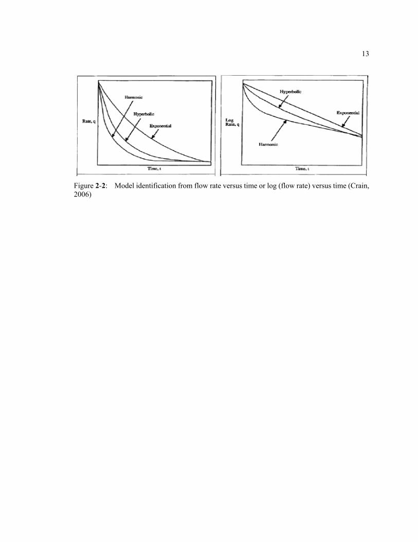
of decline curves are shown in Figure 2-2.

Exponential decline is given by:

𝑞𝑞𝑞𝑞𝑖𝑖

= 1𝑒𝑒𝐷𝐷𝑖𝑖𝑡𝑡

……………………………………………………………………………… (2.1)

where decline rate is defined as 𝐷𝐷 = − 1𝑞𝑞

× 𝑑𝑑𝑞𝑞𝑑𝑑𝑑𝑑

, in exponential model assume 𝐷𝐷 = 𝐷𝐷𝑖𝑖 = 𝑐𝑐𝑐𝑐𝑐𝑐𝑐𝑐𝑐𝑐𝑐𝑐𝑐𝑐𝑐𝑐.

Apparently, this case is unusual in real field and the prediction is most sketchy when using this

model.

Hyperbolic decline is described by:

𝑞𝑞𝑞𝑞𝑖𝑖

= 1

(1+𝑏𝑏𝐷𝐷𝑖𝑖𝑑𝑑)1𝑏𝑏

………………………………………………………………………… (2.2)

where 𝑏𝑏 exponent is defined as 𝑏𝑏 ≡𝑑𝑑�1𝐷𝐷�

𝑑𝑑𝑑𝑑 ≅ 𝑐𝑐𝑐𝑐𝑐𝑐𝑐𝑐𝑐𝑐𝑐𝑐𝑐𝑐𝑐𝑐 , generally ranges from 0 to 0.5. For

unconventional shale the associated 𝑏𝑏 should be greater than 1.

Actually, this equation is a general form describing production decline for a well,

exponential and harmonic are specific cases where the value of b is equal to 0 and 1 respectively.

7

Harmonic decline is a specific case in hyperbolic equation, which 𝑏𝑏 = 1.

𝑞𝑞𝑞𝑞𝑖𝑖

= 1(1+𝐷𝐷𝑖𝑖𝑑𝑑)

…………………………………………………………………………… (2.3)

Some plots shape can be used as a diagnostic tool to determine the type of decline before

any calculation.

2.3 Decline Curve Model for Unconventional Shale

Since we have to characterize the production behavior of the unconventional shale, a proper

model specifically designed for unconventional reservoir must be used. Duong (2011) pointed out

the fact that shale reservoirs rarely exhibits late-time flow regimes over several years but usually

displays a long-term linear flow due to the fact that the developed fracture networks caused by

pressure depletion would stimulate other pre-existed faults or fractures and further increase the

overall permeability of the reservoir. As a result, the fluid migration will be enhanced, supporting

the fracture flow over an extended time frame.

We ended up using Duong’s model (Duong, 2011) because it describes unconventional

reservoirs with very low permeability. The shape of the curve is tailored for gas wells that displays

long periods of transient flow. The Duong’s model is more conservative than traditional Arps’

hyperbolic decline curve with its hyperbolic constant b greater than unity.

𝑞𝑞 = 𝑞𝑞𝑖𝑖𝑐𝑐−𝑚𝑚 exp � 𝑎𝑎1−𝑚𝑚

(𝑐𝑐1−𝑚𝑚 − 1)� + 𝑞𝑞∞……………………………………………… (2.4)

The parameter 𝑐𝑐 and 𝑚𝑚 are determined from the log-log plot of 𝑞𝑞𝐺𝐺𝑝𝑝

vs. t (days) if we can fit

a straight line with a negative slope, −𝑚𝑚 and the intercept of 𝑐𝑐; 𝑞𝑞𝑖𝑖 is the production from day 1;

𝑞𝑞∞ is the rate at infinitive time, so it can be zero intuitively. But sometimes, since we have to

8

incorporate some effects that actually violates the ideal assumption and caused by operating

conditions in the flow rates, 𝑞𝑞∞ can be positive or negative.

2.4 Other Data-driven Machine Learning Techniques

Likewise, other data-driven and statistical machine learning methods have been developed

to assist in predicting shale gas production. According to the results from searching related papers,

those methods include but are not limited to principal component analysis (PCA), Bayesian-related

method, regression-related approaches and supportive vector machine (SVM) which classify the

data via dimensional manipulation.

Principal Component Analysis aims to decrease the dimension of the data or decompose

the features of data into several principal components that will be applied in re-creating the initial

data with reasonable accuracy (Khanal et al., 2017). The procedure can be summarized

mathematically in following condensed form:

[𝑋𝑋]𝑛𝑛×𝑚𝑚 = (𝑃𝑃𝐶𝐶1)𝑣𝑣1𝑇𝑇 + ⋯+ (𝑃𝑃𝐶𝐶𝑚𝑚)𝑣𝑣𝑚𝑚𝑇𝑇 ≈ (𝑃𝑃𝐶𝐶1)𝑣𝑣1𝑇𝑇 + ⋯+ �𝑃𝑃𝐶𝐶𝑝𝑝�𝑣𝑣𝑝𝑝𝑇𝑇 + 𝐸𝐸𝑝𝑝…………… (2.5)

In the equation above 𝑃𝑃𝐶𝐶𝑖𝑖 stands for the principal component, 𝑣𝑣𝑖𝑖𝑇𝑇 is the associated

coefficient, 𝐸𝐸𝑝𝑝 is the residual matrix between the model and measurement errors (Shlens, 2014).

Bayesian probabilistic method can be coupled with classic decline curve model like Arps’

hyperbolic curve. And reliably quantify the uncertainty in the production prediction regardless of

the decline phase (depletion stage). One featured advantage of this approach is that only production

data (flow rate) is needed in the analysis (Wang et al., 2014). This methodology is based on the

Bayes theorem shown as follows:

9

𝜋𝜋�𝜃𝜃𝑗𝑗�𝑦𝑦� =𝑓𝑓�𝑦𝑦�𝜃𝜃𝑗𝑗�𝜋𝜋�𝜃𝜃𝑗𝑗�∫𝑓𝑓�𝑦𝑦�𝜃𝜃�𝜋𝜋(𝜃𝜃)𝑑𝑑𝜃𝜃

……………………………………………………………… (2.6)

where 𝜃𝜃𝑗𝑗 is decline curve parameters, y represents flow rate data, 𝜋𝜋(𝜃𝜃𝑗𝑗) stands for prior

distribution, 𝑓𝑓�𝑦𝑦�𝜃𝜃𝑗𝑗� represents likelihood function, and the posterior probability is represented as

𝜋𝜋�𝜃𝜃𝑗𝑗�𝑦𝑦�.

Additionally, identifying organic-rich shale play (sweet spot) is another hot spot in the

research of shale gas. The application of support vector machine (SVM) helps this topic by

classifying the litho-facies efficiently with a high cross-validation accuracy (Wang et al., 2014).

Besides, high concentration of total organic carbon (TOC) is another strong indicator for a

promising drilling spot. One intuitive but handy method is multiple linear regression (MLR)

(Tahmasebi et al., 2017). This method works well for fitting the dependent variable in a high-

dimensional dataset while its mathematical form remains relatively simple.

2.5 Geostatistics Methods

As a division of statistics, geostatistics targets on spatial-temporal data in diverse subjects

including mining engineering, hydrology and petroleum geology, though it was firstly developed

for probability distribution forecast in ore exploration (Armstrong and Champigny, 1989). Kriging

is a family of geostatistical methods that predict the value of interest at a location where no

observation of the interest is made. This is achieved by interpolation using observed values at

nearby locations.

According to the first law of Geography introduced by Tobler (1970), everything is related

to everything else. But the near things are more related than distant things. As a result, Inverse

Distance Weighting (IDW) was firstly introduced:

10

�̂�𝑧 = ∑ 1𝑑𝑑𝛼𝛼

𝑛𝑛𝑖𝑖=1 𝑧𝑧𝑖𝑖………………………………………………………………………… (2.7)

where 𝑑𝑑 stands for the distance; 𝑧𝑧𝑖𝑖 is the observed value at location 𝑖𝑖; �̂�𝑧 is the predicted value at

unobserved location; 𝑐𝑐 is the total number of samples; 𝛼𝛼 is the weight governing the attribute of

the observed values with respect to the distance to the unknown spot. However, it is difficult to

determine 𝛼𝛼 and the correlation among observed values is not utilized.

Similar to IDW method, Kriging also assumes the unknown value is a weighted linear

combination of the known values. For example, ordinary kriging has the following form:

�̂�𝑧 = ∑ 𝜆𝜆𝑖𝑖𝑛𝑛𝑖𝑖=1 𝑧𝑧𝑖𝑖………………………………………………………………………… (2.8)

However, there are several assumptions in ordinary kriging: the variable 𝑧𝑧𝑖𝑖 must be normally-

distributed. Namely, the all variables in the study field should have a common mean and variance.

So we should have:

𝐸𝐸(�̂�𝑧 − 𝑧𝑧) = 0 𝑐𝑐𝑜𝑜 𝐸𝐸(∑ 𝜆𝜆𝑖𝑖𝑛𝑛𝑖𝑖=1 𝑧𝑧𝑖𝑖 − 𝑧𝑧) = 0……………………………………………… (2.9)

Besides, the coefficient 𝜆𝜆 requires more sophisticated procedure to determine. In general, we want

to find a set of 𝜆𝜆𝑖𝑖 that can correspond to the minimum variance of (�̂�𝑧 − 𝑧𝑧). That is, the following

cost function should be minimized:

𝐽𝐽 = 𝑉𝑉𝑐𝑐𝑜𝑜(�̂�𝑧 − 𝑧𝑧)……………………………………………………………………… (2.10)

In order to achieve this, the semivariance, 12𝐸𝐸(�̂�𝑧 − 𝑧𝑧)2, among different sampling values

should be modeled. Specifically, we need to fit a function that describe the spatial continuity of the

observed data 𝑧𝑧𝑖𝑖 and that consists of the variability (semivariance) of sample values at various

distances. An example of variogram (semivariance vs. lag distance) is shown in Fig. 2-3.

The associated assumptions vary with different branch of kriging methods. For example,

simple kriging assumes the mean of the true population is known; Universal kriging requires a

11

deterministic model to quantify the mean of the observed variables and we perform ordinary kriging

on the residual of the data; Co-kriging (Eq. 2.11) can borrow strength from multiple variables and

enhance the prediction reliability but it would require more estimation for the cross-correlation

among different types of parameters.

�̂�𝑧1 = �𝜆𝜆𝑖𝑖

𝑐𝑐

𝑖𝑖=1

𝑧𝑧1𝑖𝑖+�𝜆𝜆2𝑖𝑖

𝑐𝑐

𝑖𝑖=1

𝑧𝑧2𝑖𝑖 + ⋯……………………………………………………… (2.11)

12

Figure 2-1: Adsorbed and total gas contents vs. total organic content of Barnet Shale, from the T.P. Sims #2 well, Newark East field, FWB (Wang and Reed, 2009). Data from (Jarvie et al., 2004)

13

Figure 2-2: Model identification from flow rate versus time or log (flow rate) versus time (Crain, 2006)

14

Figure 2-3: An example of variogram model: red dots stand for half of the averaged squared difference between values at any two points in a kriged field; Purple curve stands for fitted model describing spatial correlation among observed values.

Chapter 3

METHODOLOGY

The proposed method consists of the following steps in general: First, we must filter and

clean production data across play to make the data truly reflect the production performance of

unconventional reservoirs; Then, a proper decline curve model is fitted to all remaining data on a

well-by-well basis; Next, a geostatistical modeling (methods in kriging family) are used to

interpolate the parameters of the decline curves at undeveloped sites where the universal co-kriging

is applied to model the correlations between wells. Finally, with the predicted mean and variance

of the parameters, we may construct the associated decline curves and forecast the EUR with

uncertainty.

3.1 Data Cleaning

Processing raw data is a common step before extracting any interesting information from

the data. In order to fit Duong’s model to the flow rates that represent the true production behavior

of the reservoir, we cleaned the data following these steps in order:

1. Drop data from vertical wells (keep only directional and horizontal well flow

rates);

2. Order flow rate by increasing date;

3. Remove values prior to completion date;

4. Remove any zero values at the beginning (before first positive value) OR remove

first value if it is positive (may be partial observation);

5. Remove data before peak production, if any left;

16

6. Check for gaps, zero-values, or large changes (as created by shut-in, re-stimulation,

etc.) in record and only keep data until first instance;

7. Throw out well if resulting record in less than 24 months long (to ensure sufficient

sample size for robust regression);

8. Normalize gas rate by perforation interval length, lateral length, or similar.

3.2 Decline Curve Analysis

Duong (2011) proposed a decline curve model that works well for unconventional

reservoirs which exhibit long periods of linear flow due to the pressure depletion within fracture

networks. It models gas rate (q) as a function of time (t) and four parameters (a, m, qi, q∞). The

four parameters are determined via two stages of sequential ordinary least squares (OLS)

regression. First, a and m are determined via OLS on:

ln � qGp�=m ln(t)+a……………………………………………………………………… (3.1)

then 𝑞𝑞𝑖𝑖 and 𝑞𝑞∞ are found by OLS regression of:

q=qitam+q∞……………………………………………………………………………… (3.2)

where

tam=t-mexp�a

1-m�t1-m-1��……………………………………………………………… (3.3)

In addition to catching the salient production traits of unconventional reservoirs, Duong’s

model is also advantageous in its numerical stability when fitting the curve. Since the four

parameters can be obtained by implementing OLS on Eq. 3.1 and Eq. 3.2 respectively, they are

guaranteed to be the solution of the global minimum of the squared error surface. This feature

17

makes the fitting procedure faster than those using Arps’ hyperbolic model which is done by

nonlinear regression where the global minimum of squared error cannot be ensured even after many

iterations.

3.3 Geostatistics Method

To calculate EUR at undrilled sites, we must first predict the associated parameters based

on known data points. Although a variety of mathematical interpolation techniques are available,

such as spline and polynomial, the spatial correlation among observations is ignored in them.

Therefore, methods from the kriging family that will handle the underlying spatial structures are

applied in our work.

Intuitively, the four parameters (a, m, qi, q∞) for each well should be mutually related

because they collectively quantify the same decline curve. Meanwhile, a more reliable estimation

can be obtained by utilizing the spatial correlation between different variables (Trangmar et al.,

1986). Thus, co-kriging is employed in our work, which exploits the (potential) cross-correlation

between the four decline curve parameters and their joint spatial correlation simultaneously. Co-

kriging is a well-established procedure and details on this method can be found in many books

(Journel and Huijbregts, 1978; McBratney and Webster, 1983; Vauclin et al., 1983). While co-

kriging takes advantage of multiple parameters, large-scale spatial trends in the data (external drift)

need to be accounted for before kriging. This idea is conveyed from universal kriging that allows

the kriging in the presence of nonstationarity (Matheron, 1971). Therefore, we should utilize the

features of the two kriging methods by “filtering out” the external drift from the data first and then

co-kriging the associated residuals, which leads to an indirect but comprehensive hybrid method,

“universal co-kriging”.

18

With the goal being to construct maps of decline curve parameters and subsequently EUR

over the spatial domain of the play, it is appropriate to perform this universal co-kriging on blocks

rather than specific points. The size of the block should be chosen to balance utility of the resulting

map and computation time; the size should be at a useful scale to support operational decisions and

give sufficient spatial resolution, however too many blocks results in large memory and

computational time requirements for the kriging process, and may give an unnecessary level of

detail. Here, we recommend scaling the blocks to be roughly twice the average lateral length, such

that if a well pad were placed in the center of a block, the lateral(s) would still be contained within

the block, unless chosen to be exceedingly long. In “block kriging” the mean and variance of the

predicted parameters are determined for each block. Since we perform co-kriging, the co-variances

are determined as well. Thus, we can determine the P10, P50 and P90 EUR by numerically

integrating Duong’s decline curve with its parameters sampled from a multivariate normal

distribution. To better explain this integrated approach, a case study on the Marcellus shale is

presented in the following section.

Chapter 4

CASE STUDY

4.1 Data Source

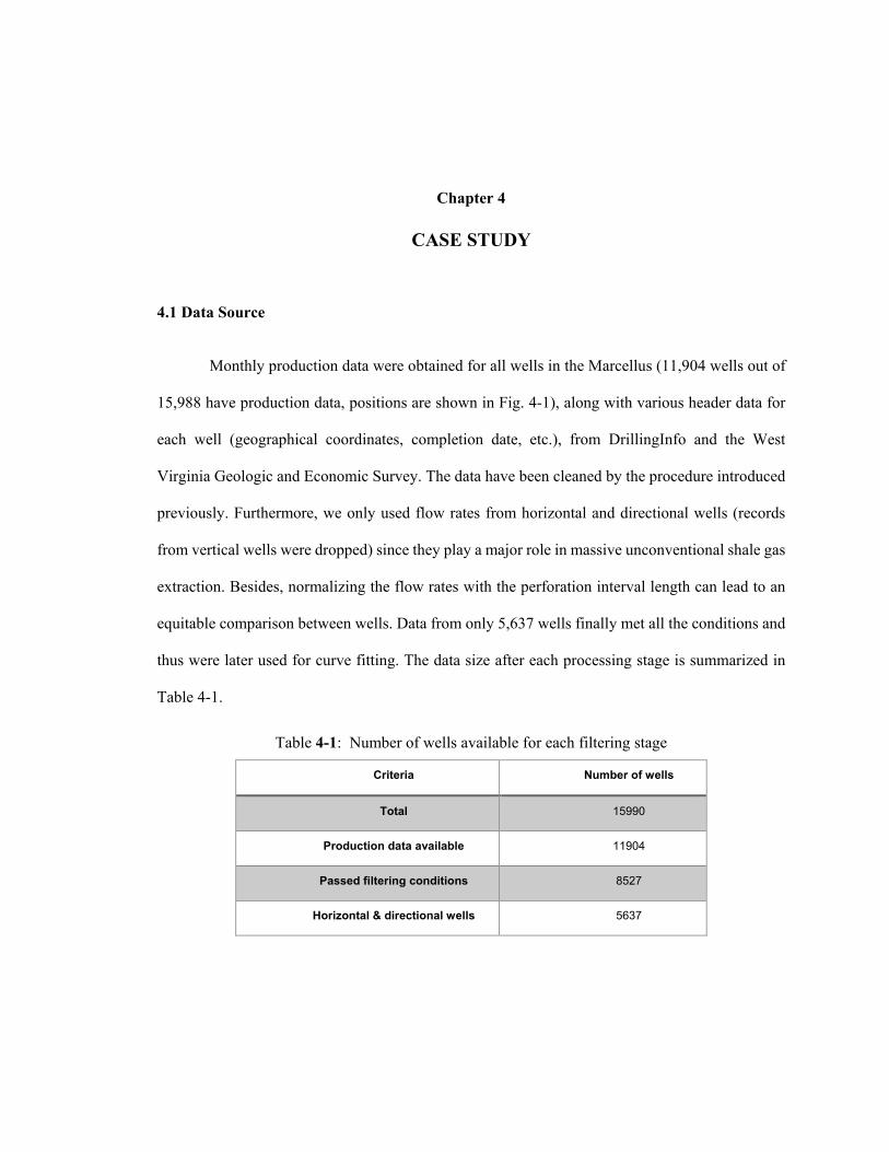
Monthly production data were obtained for all wells in the Marcellus (11,904 wells out of

15,988 have production data, positions are shown in Fig. 4-1), along with various header data for

each well (geographical coordinates, completion date, etc.), from DrillingInfo and the West

Virginia Geologic and Economic Survey. The data have been cleaned by the procedure introduced

previously. Furthermore, we only used flow rates from horizontal and directional wells (records

from vertical wells were dropped) since they play a major role in massive unconventional shale gas

extraction. Besides, normalizing the flow rates with the perforation interval length can lead to an

equitable comparison between wells. Data from only 5,637 wells finally met all the conditions and

thus were later used for curve fitting. The data size after each processing stage is summarized in

Table 4-1.

Table 4-1: Number of wells available for each filtering stage

Criteria Number of wells

Total 15990

Production data available 11904

Passed filtering conditions 8527

Horizontal & directional wells 5637

20

4.2 Parameter Visualization

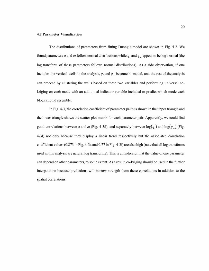
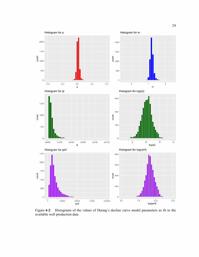
The distributions of parameters from fitting Duong’s model are shown in Fig. 4-2. We

found parameters a and m follow normal distributions while qi and q∞ appear to be log-normal (the

log-transform of these parameters follows normal distributions). As a side observation, if one

includes the vertical wells in the analysis, qi and q∞ become bi-modal, and the rest of the analysis

can proceed by clustering the wells based on these two variables and performing universal co-

kriging on each mode with an additional indicator variable included to predict which mode each

block should resemble.

In Fig. 4-3, the correlation coefficient of parameter pairs is shown in the upper triangle and

the lower triangle shows the scatter plot matrix for each parameter pair. Apparently, we could find

good correlations between a and m (Fig. 4-3d), and separately between log�qi� and log�q∞� (Fig.

4-3l) not only because they display a linear trend respectively but the associated correlation

coefficient values (0.873 in Fig. 4-3a and 0.77 in Fig. 4-3i) are also high (note that all log transforms

used in this analysis are natural log transforms). This is an indicator that the value of one parameter

can depend on other parameters, to some extent. As a result, co-kriging should be used in the further

interpolation because predictions will borrow strength from these correlations in addition to the

spatial correlations.

4.3 External Drift

To ensure the stationarity of our data before geostatistical modeling, we can fit a

background trend (external drift) for universal kriging. Because we have r multiple response

variables (in this case, the four decline curve parameters) and p multiple explanatory variables (in

this case, spatial coordinates x and y, which are the UTM Eastings and Northings (both in km),

respectively, plus an interaction term xy), we fit a multivariate multiple linear regression model for

the background trend:

where Y is an n × r matrix (n being the number of observations, or wells in this application)

containing each response variable as a column, Z is an n × (p+1) matrix containing the explanatory

variables plus a series of ones (for fitting an intercept) as columns, β is a (p+1) × r matrix

containing the regression coefficients, and ε is an n × m matrix of error terms. The regression

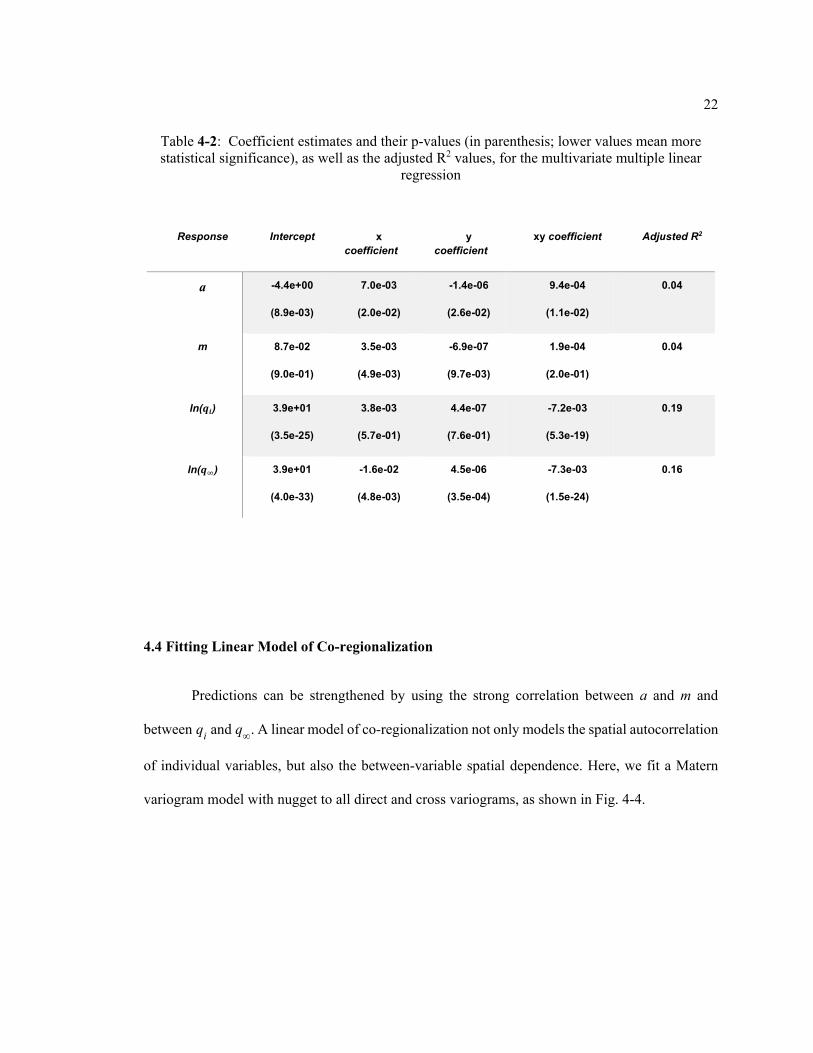
coefficient estimates, their p-values, and the adjusted R2 values are reported in Table 4-2.

Table 4-2 shows that while the adjusted R2 values are fairly low for all four models, the

coefficients are generally significant (low p-values), albeit also generally low in magnitude.

Nevertheless, these models have better adjusted goodness-of-fit (higher R2) than simpler models

with fewer terms, including models of just an intercept (mean; as would be used for simple kriging).

This criteria of higher adjusted R2 is the reason for including the interaction term, xy.

Y = βZ+ε……………………………………………………………………………… (4.1)

22

4.4 Fitting Linear Model of Co-regionalization

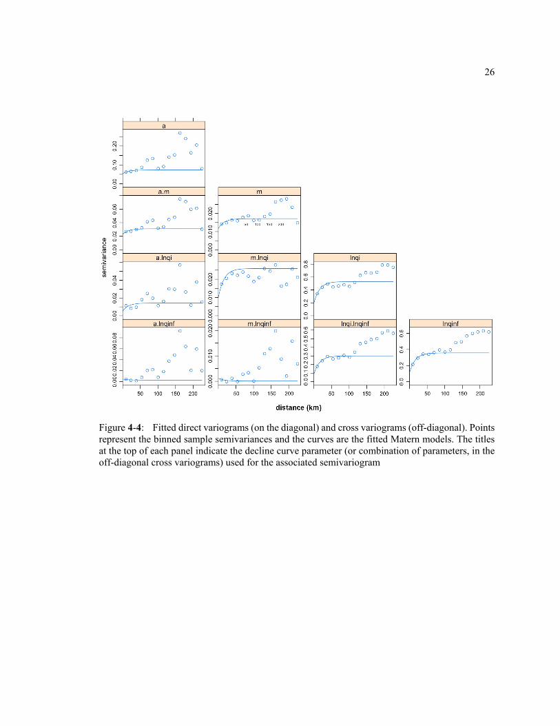
Predictions can be strengthened by using the strong correlation between a and m and

between qi and q∞. A linear model of co-regionalization not only models the spatial autocorrelation

of individual variables, but also the between-variable spatial dependence. Here, we fit a Matern

variogram model with nugget to all direct and cross variograms, as shown in Fig. 4-4.

Table 4-2: Coefficient estimates and their p-values (in parenthesis; lower values mean more statistical significance), as well as the adjusted R2 values, for the multivariate multiple linear

regression

Response Intercept x coefficient

y coefficient

xy coefficient Adjusted R2

a -4.4e+00

(8.9e-03)

7.0e-03

(2.0e-02)

-1.4e-06

(2.6e-02)

9.4e-04

(1.1e-02)

0.04

m 8.7e-02

(9.0e-01)

3.5e-03

(4.9e-03)

-6.9e-07

(9.7e-03)

1.9e-04

(2.0e-01)

0.04

ln(𝒒𝒒𝒒𝒒) 3.9e+01

(3.5e-25)

3.8e-03

(5.7e-01)

4.4e-07

(7.6e-01)

-7.2e-03

(5.3e-19)

0.19

ln(𝒒𝒒∞) 3.9e+01

(4.0e-33)

-1.6e-02

(4.8e-03)

4.5e-06

(3.5e-04)

-7.3e-03

(1.5e-24)

0.16

23

Figure 4-1: Marcellus well locations in the study area (Data Source: DrillingInfo, West Virginia Geological and Economic Survey). Wells denoted with blue points have production data and are used in the analysis in this paper (red points do not have available data)

24

Figure 4-2: Histograms of the values of Duong’s decline curve model parameters as fit to the available well production data

Figure 4-3: Scatter plot for fitted decline curve parameters (lower triangular part) and associated correlation coefficient values (upper triangular part). Each scatter-plot panel corresponds to its correlation coefficient in a mirror position (e.g., panel d is associated with the value in panel a)

26

Figure 4-4: Fitted direct variograms (on the diagonal) and cross variograms (off-diagonal). Points represent the binned sample semivariances and the curves are the fitted Matern models. The titles at the top of each panel indicate the decline curve parameter (or combination of parameters, in the off-diagonal cross variograms) used for the associated semivariogram

Chapter 5

RESULTS AND DISCUSSION

5.1 Block Co-kriging with External Drift

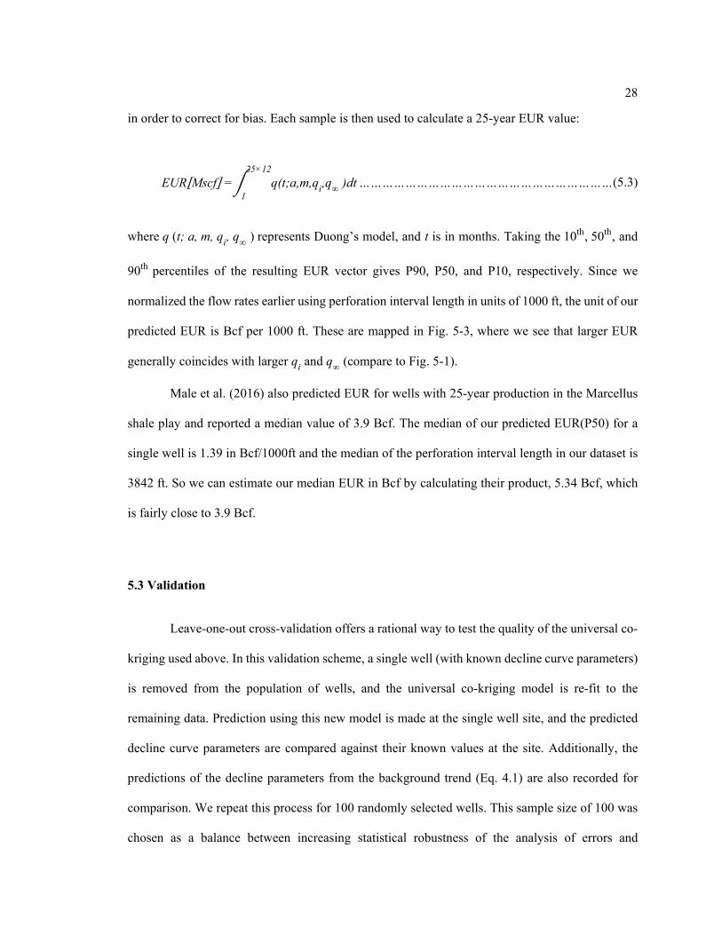
Fig. 5-1 and Fig. 5-2 show the mean and variance respectively of each decline curve

parameter. They are estimated within 5 km × 5 km blocks spanning the domain of the Marcellus.

The noticeably low a and m predictions in the northern part of the Marcellus are controlled by two

wells: API 37-105-21728 and 37-105-21722, which show radically sharp decline after 3 months.

One can also see that larger qi and q∞ values generally exist around southwest Pennsylvania and

around Bradford county, PA, in the northeast (Fig. 5-1). Fig. 5-2 shows small variances for all

parameters in proximity to existing well locations, and increasingly large variances towards the

fringe of the Marcellus, with the largest values in the far southwest and northern extents.

5.2 Estimated Ultimate Recovery

Estimated Ultimate Recovery EUR (at P10, P50, and P90 levels) is estimated by drawing

a random sample of size 1,000 from a multivariate normal distribution for a, m, ln�qi�, and ln�q∞�.

The mean values and covariance matrix are constructed from the universal co-kriging predicted

values in each block. The samples of the log-transformed variables are back-transformed via:

qi= exp�ln�qi�+0.5�var�ln�qi����…………………………………………………………… (5.2)

q∞= exp�ln�q∞�+0.5�var�ln�q∞����………………………………………………………… (5.1)

28

in order to correct for bias. Each sample is then used to calculate a 25-year EUR value:

where q (t; a, m, qi, q∞ ) represents Duong’s model, and t is in months. Taking the 10th, 50th, and

90th percentiles of the resulting EUR vector gives P90, P50, and P10, respectively. Since we

normalized the flow rates earlier using perforation interval length in units of 1000 ft, the unit of our

predicted EUR is Bcf per 1000 ft. These are mapped in Fig. 5-3, where we see that larger EUR

generally coincides with larger qi and q∞ (compare to Fig. 5-1).

Male et al. (2016) also predicted EUR for wells with 25-year production in the Marcellus

shale play and reported a median value of 3.9 Bcf. The median of our predicted EUR(P50) for a

single well is 1.39 in Bcf/1000ft and the median of the perforation interval length in our dataset is

3842 ft. So we can estimate our median EUR in Bcf by calculating their product, 5.34 Bcf, which

is fairly close to 3.9 Bcf.

5.3 Validation

Leave-one-out cross-validation offers a rational way to test the quality of the universal co-

kriging used above. In this validation scheme, a single well (with known decline curve parameters)

is removed from the population of wells, and the universal co-kriging model is re-fit to the

remaining data. Prediction using this new model is made at the single well site, and the predicted

decline curve parameters are compared against their known values at the site. Additionally, the

predictions of the decline parameters from the background trend (Eq. 4.1) are also recorded for

comparison. We repeat this process for 100 randomly selected wells. This sample size of 100 was

chosen as a balance between increasing statistical robustness of the analysis of errors and

EUR[Mscf] =� q(t;a,m,qi,q∞ )dt25×12

1………………………………………………………… (5.3)

29

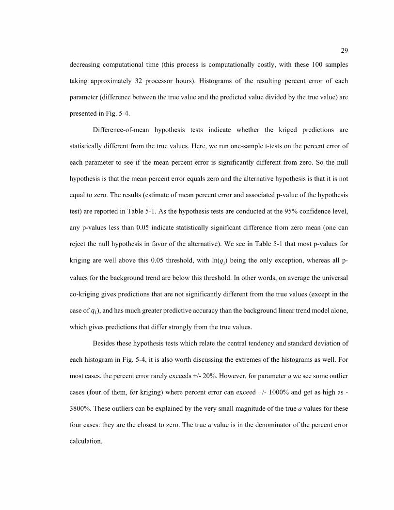
decreasing computational time (this process is computationally costly, with these 100 samples

taking approximately 32 processor hours). Histograms of the resulting percent error of each

parameter (difference between the true value and the predicted value divided by the true value) are

presented in Fig. 5-4.

Difference-of-mean hypothesis tests indicate whether the kriged predictions are

statistically different from the true values. Here, we run one-sample t-tests on the percent error of

each parameter to see if the mean percent error is significantly different from zero. So the null

hypothesis is that the mean percent error equals zero and the alternative hypothesis is that it is not

equal to zero. The results (estimate of mean percent error and associated p-value of the hypothesis

test) are reported in Table 5-1. As the hypothesis tests are conducted at the 95% confidence level,

any p-values less than 0.05 indicate statistically significant difference from zero mean (one can

reject the null hypothesis in favor of the alternative). We see in Table 5-1 that most p-values for

kriging are well above this 0.05 threshold, with ln(qi) being the only exception, whereas all p-

values for the background trend are below this threshold. In other words, on average the universal

co-kriging gives predictions that are not significantly different from the true values (except in the

case of 𝑞𝑞𝑖𝑖), and has much greater predictive accuracy than the background linear trend model alone,

which gives predictions that differ strongly from the true values.

Besides these hypothesis tests which relate the central tendency and standard deviation of

each histogram in Fig. 5-4, it is also worth discussing the extremes of the histograms as well. For

most cases, the percent error rarely exceeds +/- 20%. However, for parameter a we see some outlier

cases (four of them, for kriging) where percent error can exceed +/- 1000% and get as high as -

3800%. These outliers can be explained by the very small magnitude of the true a values for these

four cases: they are the closest to zero. The true a value is in the denominator of the percent error

calculation.

30

5.4 Geological Interpretation

Several authors (Wrightstone, 2009; Erenpreiss et al., 2011; Wang and Carr, 2013; EIA,

2017) have conducted geological mapping in the Marcellus shale on its depth, thickness, and

thermal maturity (Fig. 5-5 and Fig. 5-6 left sides), which helps interpret the P50 EUR heatmap

constructed in our study. From a geological perspective on unconventional plays, high

hydrocarbon-generation potential and a large thickness of the source rock can attribute to a high

gas production (Zou et al., 2010; Mallick and Achalpurkar, 2014). Also, the thermal maturity is a

key factor of the hydrocarbon-generation potential, and is correlated to formation depth because of

the geothermal and pressure gradients (the Marcellus formation top contour versus thermal maturity

zones in Fig. 5-5 left side). In the overmature zone and those within the gas generation window

(gas prone), an in-situ natural gas accumulation region could be formed (the gray and pink zone in

Fig. 5-5 left side) while a considerable amount of natural gas reserve is unlikely to be found in the

Table 5-1: One-sample t-test results for each decline curve parameter and for both the universal co-kriging predictions and background trend predictions

Krige Trend

Parameter Mean p-value Mean p-value

a -3.62 0.94 107.37 0.003

m -0.44 0.53 2.32 0.006

ln(𝑞𝑞𝑖𝑖) 9.79 7.56E-36 13.97 5.63E-45

ln(𝑞𝑞∞) -0.10 0.83 4.44 6.35E-09

31

immature zone (the light-yellow area in Fig. 5-5 left side). That is, high gas production from the

wells located in the middle of the play should result from the source rock that tends to generate

more gas than oil; The wells in the northeast should produce a significant amount of dry gas from

overmatured shale; Similarly, abundant yields of dry gas could be found along the southwest

boundary of the play despite few wells, so far, have been drilled there. Additionally, a larger

thickness the source rock has, the more hydrocarbon-productive kerogens it may bear. Thus, the

shale thickness is another critical factor to assess the production potential. In Fig. 5-6, the P50 EUR

heatmap (right side) has revealed that high-yield areas mentioned above (middle, northeast,

southwest) always show up in the bright-green and pink zones in the isopach (Fig. 5-6 left side)

where the associated Marcellus shale gross thickness is considerable.

On the other hand, the low EUR areas (blue areas) in the northeast part of the Marcellus

shale could result from both thin shale and less matured shale. Since a smaller thickness the shale

has, the less hydrocarbon it can potentially produce. Besides, a lower vitrinite reflectance can result

in a smaller gas production as long as the shale has not reached the gas window due to either/both

low geothermal gradient or/and shallow burial depth.

As a result, the high EUR zones in our results are located in the northeast, middle and

southeast part in our mapping area sharing similar locations with high thermal maturity and great

thickness (see comparisons in Fig. 5-5 and Fig. 5-6). In other words, our production forecasts and

reserves estimates are in agreement with the associated geological evidence. Besides qualitatively

validating the heatmap with geological variables, it should be beneficial to incorporate them as

additional inputs in co-kriging to strengthen predictions of the decline curve parameters for

undrilled wells, taking advantage of the spatial correlations among geological variables.

Specifically, we may add the shale thickness, vitrinite reflectance (%Ro), etc. at operating well

sites as one of the dependent variables in co-kriging interpolation, and use maps of such properties

32

away from the wells to increase the accuracy of, and reduce uncertainty in, our decline curve

parameter predictions.

5.5 Web Application

In order to increase the transparency of this work and make the findings available in a

comprehensive format, we have created a web application which can be accessed via the link:

https://shinysrv.ems.psu.edu/eum19/Virtual_Asset_1_0/. This utility allows one to click anywhere

in the Marcellus to view the predicted decline curves (P10, P50, P90), along with specific EUR

values for the selected block. Furthermore, one can view the fitted decline curve parameter values

(as well as goodness-of-fit) at each well in geographical format. One example is shown in Fig. 5-

7.

33

Figure 5-1: Predicted mean for each type of parameters of Duong’s decline curve model: Panel a.) b.) c.) d.) show the mean values for 𝒂𝒂, 𝒎𝒎, 𝐥𝐥𝐥𝐥𝐥𝐥(𝒒𝒒𝒒𝒒), 𝐥𝐥𝐥𝐥𝐥𝐥(𝒒𝒒𝒒𝒒𝒒𝒒𝒒𝒒) repectively (all log transforms used in this analysis are natural log transforms) (Legends in the right corner: left one for dots or existing well sites, right one for grids or undeveloped sites). Well location data are from WVGES and DrillingInfo

Figure 5-2: Predicted variance for each type of parameters of Duong’s decline curve model: Panel a.) b.) c.) d.) show the variances for 𝒂𝒂, 𝒎𝒎, 𝐥𝐥𝐥𝐥𝐥𝐥(𝒒𝒒𝒒𝒒), 𝐥𝐥𝐥𝐥𝐥𝐥(𝒒𝒒𝒒𝒒𝒒𝒒𝒒𝒒) repectively (all log transforms used in this analysis are natural log transforms)

35

Figure 5-3: Predicted EUR heatmaps across the Marcellus shale. Panel a.), b.), and c.) stand for P10, P50, and P90 EUR respectively. The units are BCF per 1000 ft. of interval length

36

Figure 5-4: Histograms of percent error for each decline curve parameter and each method: universal co-kriging (dark grey) and background trend (light grey). The decline curve parameter is indicated at the top of each frame. Note that the x- and y-axis scales vary from frame-to-frame

37

Figure 5-5: Thermal maturity and initial yields in the Marcellus shale is shown at the left side: The light-yellow area stands for immature zone; Green zone shows oil prone; Pink zone represents gas prone; Gray zone stands for overmature zone. At the right side, the heatmap of predicted P50 EUR indicates high-production areas (orange-red) tend to be located within gas-prone zone and overmature zone where gas is the major product from the source rock (e.g., the northeastern high EUR area mainly exist within the overmature zone). (left-side figure source: U.S. Energy Information Administration based on DrillingInfo, and U.S. Geological Survey)

38

Figure 5-6: Color-filled Marcellus isopach (Wang and Carr, 2013) is shown at the left side where the formation thickness increases as the color varies from light-green to bright-green to pink. At the right side, the heatmap of predicted P50 EUR indicates high-production areas (orange-red) show up in the areas with considerable shale thickness (see the isopach). These areas include the northeast, middle and southeast boundary of the entire shale play

39

Figure 5-7: One example of predicted decline curves and the associated EUR values at a single undeveloped well site (labeled with a black star) where the dots shown in this map represent existing well sites only.

Chapter 6

SUMMARY AND CONCLUSION

The approach we are proposing in this paper is a combination of decline curve analysis and

geostatistical methods. First, the parameters that describe the natural gas production variation are

obtained by decline curve fitting. According to their statistics, we can choose a proper geostatistical

method (universal co-kriging) to interpolate those parameters for undrilled sites. Finally, we can

estimate the EUR and associated decline curve with predicted parameters while quantifying the

uncertainty at the same time. Without asking for extensive types of data, our approach is handy to

implement and can provide operators with a good reference for early-stage explorations.

The median value of our predicted EUR (P50) is close to that reported by other authors

(Male et al., 2016). The heatmaps generated in our case study have shown that the promising sites

with high EUR are mainly located in the middle and northeast of the study area, which is consistent

with other geological evidence in the Marcellus. Although some areas along the southeast boundary

of the EUR heatmap also appear to be sweet spots, the reliability of their EUR may suffer from the

relatively high variance of the associated decline curve parameters. Furthermore, the validation not

only indicates the superiority of the universal co-kriging over the background trend prediction but

also shows reasonable percent errors in predicted parameters despite the “magnitude” issue for

parameter a.

Lastly, some extensions and modifications may be applied in our future work such as

adopting modified Duong’s model (Joshi and Lee, 2013) to avoid potentially unrealistic forecasts

or employing pattern recognition method (unsupervised learning) to further narrow down the range

of promising areas based upon our current analysis. Besides, given the production data associated

41

with the recording time, we can create EUR heatmaps following along the discretized time frames

so that we can explore the EUR (predicted) increment due to the advance of production techniques.

REFERENCES

Anderson, D. M., and P. Liang, 2011, Quantifying Uncertainty in Rate Transient Analysis for

Unconventional Gas Reservoirs: the SPE North American Unconventional Gas Conference

and Exhibition, p. 14–16 June. SPE 145088–MS, doi:10.2118/145088-MS.

Armstrong, M., and N. Champigny, 1989, A study on kriging small blocks: CIM BULLETIN, v.

82, no. 923, p. 128–133.

Arps, J. J., 1945, Analysis of Decline Curves: Transactions of the AIME, doi:10.2118/945228-G.

Belvalkar, R. A., and S. Oyewole, 2010, Development of Marcellus Shale in Pennsylvania, in

SPE Annual Technical Conference and Exhibition, Florence, Italy: Society of Petroleum

Engineers, doi:10.2118/134852-MS.

Bhattacharya, S., and M. Nikolaou, 2013, Analysis of Production History for Unconventional Gas

Reservoirs With Statistical Methods: SPE, doi:10.2118/147658-PA.

Blasingame, T. A., 2008, The Characteristic Flow Behavior of Low-Permeability Reservoir

Systems, in SPE Unconventional Reservoirs Conference, Keystone, Colorado, USA:

Society of Petroleum Engineers, doi:10.2118/114168-MS.

Blatt, H., R. J. Tracy, and E. G. Ehlers, 1996, Petrology: igneous, sedimentary, and metamorphic:

New York, W.H. Freeman, 529 p.

Bustin, R. M., A. M. M. Bustin, A. Cui, D. Ross, and V. M. Pathi, 2008, Impact of Shale

Properties on Pore Structure and Storage Characteristics, in SPE Shale Gas Production

Conference, Fort Worth, Texas, USA: Society of Petroleum Engineers,

doi:10.2118/119892-MS.

43

Cipolla, C. L., E. P. Lolon, J. C. Erdle, and B. Rubin, 2010, Reservoir Modeling in Shale-Gas

Reservoirs: SPE Reservoir Evaluation & Engineering, doi:10.2118/125530-PA.

Clarkson, C. R., J. L. Jensen, and S. Chipperfield, 2012, Unconventional gas reservoir evaluation:

What do we have to consider? Journal of Natural Gas Science and Engineering,

doi:10.1016/j.jngse.2012.01.001.

Crain, E. R., 2006, Crain’s Petrophysical Pocket Pal: ER Ross Ontario.

Davies, D. K., W. R. Bryant, R. K. Vessell, and P. J. Burkett, 1991, Porosities, permeabilities,

and microfabrics of Devonian shales, in Microstructure of fine-grained sediments: Springer,

p. 109–119.

Diaz De Souza, O. C., A. Sharp, R. C. Martinez, R. A. Foster, E. Piekenbrock, M. Reeves

Simpson, and I. Abou-Sayed, 2012, Integrated Unconventional Shale Gas Reservoir

Modeling: A Worked Example From the Haynesville Shale, De Soto Parish, North

Louisiana, in SPE Americas Unconventional Resources Conference: doi:10.2118/154692-

MS.

Duong, A. N., 2011, Rate-decline analysis for fracture-dominated shale reservoirs: SPE Reservoir

Evaluation & Engineering, v. 14, no. 03, p. 377–387.

EIA (Energy Information Administration), U.S. Department of Energy, Independent Statistics &

Analysis, 2017, Marcellus Shale Play Geology review, Retrieved from

https://www.eia.gov/maps/pdf/MarcellusPlayUpdate_Jan2017.pdf

Erenpreiss, M. S., M. Rd, B. C-, and W. Virginia, 2011, Mapping the Regional Organic

Thickness of the “ Marcellus Shale ,” Hamilton Group ABSTRACT • Regional and

statewide isopach maps have been developed for the Middle Devonian “ Marcellus Shale ”

for use in assessing Ohio ’ s shale gas potential . Existing s: p. 2011.

Erdle, J., Hale, B., Houze, O., Ilk, D., Jenkins, C., Lee, W. J., Ritter, J., Seidle, J. P., and Wilson,

S. 2016. Monograph 4: Estimating Ultimate Recovery of Developed Wells in Low-

44

Permeability Reservoirs. Society of Petroleum Evaluation Engineers.

Freeman, C., G. J. Moridis, D. Ilk, and T. Blasingame, 2010, A Numerical Study of Transport and

Storage Effects for Tight Gas and Shale Gas Reservoir Systems, in International Oil and

Gas Conference and Exhibition in China, Beijing, China: Society of Petroleum Engineers,

doi:10.2118/131583-MS.

Hauge, V. L., and G. H. Hermansen, 2017, Machine Learning Methods for Sweet Spot Detection:

A Case Study BT - Geostatistics Valencia 2016, in J. J. Gómez-Hernández, J. Rodrigo-

Ilarri, M. E. Rodrigo-Clavero, E. Cassiraga, and J. A. Vargas-Guzmán, eds.: Cham, Springer

International Publishing, p. 573–588, doi:10.1007/978-3-319-46819-8_38.

Jarvie, D., R. M. Pollastro, R. J. Hill, K. A. Bowker, B. L. Claxton, and J. Burgess, 2004,

Evaluation of hydrocarbon generation and storage in the Barnett shale, Ft. Worth basin,

Texas, in Ellison Miles Memorial Symposium, Farmers Branch, Texas, USA: p. 22–23.

Joshi, K., and J. Lee, 2013, Comparison of Various Deterministic Forecasting Techniques in

Shale Gas Reservoirs: SPE Conference, p. 12, doi:10.2118/163870-MS.

Journel, A. G., and C. J. Huijbregts, 1978, Mining geostatistics: Academic press.

Khanal, A., M. Khoshghadam, W. J. Lee, and M. Nikolaou, 2017, New forecasting method for

liquid rich shale gas condensate reservoirs with data driven approach using principal

component analysis: Journal of Natural Gas Science and Engineering, v. 38, p. 621–637.

Kothari, N., 2011, An Unconventional Energy Resources: Shale Gas, in Offshore Mediterranean

Conference and Exhibition: Offshore Mediterranean Conference.

Luffel, D. L., and F. K. Guidry, 1992, New Core Analysis Methods for Measuring Reservoir

Rock Properties: p. 7.

Male, F., M. P. Marder, J. Browning, S. Ikonnikova, and T. Patzek, 2016, Marcellus Wells’

Ultimate Production Accurately Predicted from Initial Production: SPE Low Perm

Symposium, no. January 2015, doi:10.2118/180234-MS.

45

Mallick, M., and M. P. Achalpurkar, 2014, Factors Controlling Shale Gas Production: Geological

Perspective, in Abu Dhabi International Petroleum Exhibition and Conference: p. 10–13,

doi:10.2118/171823-MS.

Matheron, G., 1971, The theory of regionalised variables and its applications: Les Cahiers du

Centre de Morphologie Mathématique, v. 5, p. 212.

McBRATNEY, A. B., and R. WEBSTER, 1983, Optimal interpolation and isarithmic mapping of

soil properties: V. Co‐regionalization and multiple sampling strategy: Journal of Soil

Science, doi:10.1111/j.1365-2389.1983.tb00820.x.

Moinfar, A., A. Varavei, K. Sepehrnoori, and R. T. Johns, 2013, Development of a Coupled Dual

Continuum and Discrete Fracture Model for the Simulation of Unconventional Reservoirs,

in SPE Reservoir Simulation Symposium: doi:10.2118/163647-MS.

Oliver, D. S., and Y. Chen, 2011, Recent progress on reservoir history matching: A review:

doi:10.1007/s10596-010-9194-2.

Ozdemir, I., Q. Sun, and T. Ertekin, 2016, Structuring an Integrated Reservoir Characterization

and Field Development Protocol Utilizing Artificial Intelligence: Proceedings of the 26th

ITU Petroleum and Natural Gas Symposium and Exhibition.

Reed, R. M., A. John, and G. Katherine, 2007, Nanopores in the Mississippian Barnett shale:

Distribution, morphology, and possible genesis, in GSA Denver Annual Meeting: p. 358.

Sakhaee-Pour, A., and S. L. Bryant, 2012, Gas Permeability of Shale: p. 9.

Shlens, J., 2014, A tutorial on principal component analysis. arXiv preprint arXiv: 14041100.

Soeder, D. J., 1988, Porosity and Permeability of Eastern Devonian Gas Shale: SPE Formation

Evaluation, v. 3, no. 01, p. 116–124, doi:10.2118/15213-PA.

Trangmar, B. B., R. S. Yost, and G. Uehara, 1986, Application of Geostatistics to Spatial Studies

of Soil Properties: Advances in Agronomy, doi:10.1016/S0065-2113(08)60673-2.

Vauclin, M., S. R. Vieira, G. Vachaud, and D. R. Nielsen, 1983, The Use of Cokriging with

46

Limited Field Soil Observations 1: Soil Science Society of America Journal, v. 47, no. 2, p.

175–184.

Wang, G., and T. R. Carr, 2013, Organic-rich marcellus shale lithofacies modeling and

distribution pattern analysis in the appalachian basin: AAPG Bulletin, v. 97, no. 12, p.

2173–2205, doi:10.1306/05141312135.

Wang, G., T. R. Carr, Y. Ju, and C. Li, 2014, Identifying organic-rich Marcellus Shale lithofacies

by support vector machine classifier in the Appalachian basin: Computers & Geosciences,

v. 64, p. 52–60.

Wang, F. P., and R. M. Reed, 2009, Pore Networks and Fluid Flow in Gas Shales, in SPE Annual

Technical Conference and Exhibition, New Orleans, Louisiana: Society of Petroleum

Engineers, doi:10.2118/124253-MS.

Wrightstone, G. R., 2009, Marcellus Shale - geologic controls on production: Search and

Discovery, v. 10206, p. 1–10.

Wu, Y.-S., J. Li, D. Ding, C. Wang, and Y. Di, 2014, A Generalized Framework Model for the

Simulation of Gas Production in Unconventional Gas Reservoirs: SPE Journal, v. 19, no.

05, p. 845–857, doi:10.2118/163609-PA.

Zou, C., D. Dong, S. Wang, J. Li, X. Li, Y. Wang, D. Li, and K. Cheng, 2010, Geological

characteristics and resource potential of shale gas in China: Petroleum Exploration and

Development, v. 37, no. 6, p. 641–653, doi:10.1016/S1876-3804(11)60001-3.