Embed Size (px)
Citation preview
University of Missan
College of Engineering
Petroleum Engineering Department
MATEREAL BALANCE AND DECLINE CURVE
ANALYSIS TO PREDICTION THE PERFORMANCE
OF RESERVOIR USING MBAL SOFTWERE
BY
Hussein Fadhil Abed
Kawther Abdullah
Wasan Naaem
Supervisor
Dr. Ahmed Kadhim
2018

I
DIDICATION
We wish to dedicate this work to our parents, brother, sister and martyrs
of Iraq who sacrifice to continue the life.

II
ACKNOWLEDMENT
On this occasion we would like to extolment the Lord of cosmos (Allah),
for what he gave me strength, talent, mind and opportunity to complete my
study.
At this opportunity we would like to express my most sincere gratitude and
appreciation to our supervisor Dr. Ahmed Kadhim for his valuable guidance
and genuine interest as research advisor.
III
Abstract
Predicting the performance of reservoirs by estimating the initial oil in
place, the recoverable hydrocarbon and prediction the future production can
gives the adequate understand to the reservoir engineers to developing good
planning to enhanced oil recovery.
In this work, software called MBAL was used to compute the oil originally
in place by performing a nonlinear regression of average pressure against
cumulative oil production and to perform different scenarios of reservoir
performance predictions. The data that used in this study is from L.P Dake
(example 9.2). The value of OIIP that determined by MBAL software in this
study was 313.093 MMSTB and this value is very close to the measured
value in L.P Dake example 9.2 (312 MM STB). The proved recoverable
hydrocarbon from 1998 to the end of production using exponential decline
was 20.99 while Cumulative production before the study period and the
cumulative production in the future result from decline curve is 20.99+29.15
=50.14 MMSTB. This result represents the proved reserve that will produced
by The natural energy of the reservoir. While the probable reserves maybe
produced determine from hyperbolic decline is about 21.4 MMSTB.
The future performance show When starting injection water from year 2004
to 2010 with flow rate 20000 STB/D the pressure decrees from 1440 psia to
1413.46 psia and the cumulative oil produced 94.7305 MM STB. When make
injection with flow rate 40000 STB/D the pressure increase from 1440 psia
at 2004 to 2030.65 psia at 2010 and the cumulative oil produced 94.7305
STB/D.
Also we use decline curve analysis to predict the remains recoverable and
future production for three wells from data taken from Iraqi fields
IV
Table of Contents
Dedication ……………………………………………………….……… I
Acknowledgment ……………………………………………….………II
Abstract ….……………………………………………………….……. III
Table of Contents ………………………………………….……………IV
List of Tables ……………………………………………………………VII
List of Figures ……………………………………………………….… VIII
Nomenclature and Abbreviations ……………………………….……....X
Chapter one
INTERDUCTION
1-1 Background of the Study ….……………………………….…… 1
1-1-1 Material Balance ….………………….…………………………2
1-1-2 Decline Curve ….….…………………….……………….………3
1-2 Objectives of the Study …………………………………….……....4
Chapter Two
Literature Review
2-1 Material Balance …………………………………...……………….5
2-1-1 Material Balance Theory ………………………………………….7
2-1-2 Derivative of Material Balance Equation ………………………......7
2.1.3 Material balance equation as straight line ……………………......17
2-1-4 The Straight-Line Solution Method to The MBE ……….……......18
2-2 Decline curve ………………………….…………………………….22
2-2-1 Golden rule of DCA …………………………………………...….23
2-2-2 History of DCA …………………………………….......…….….23
2-2-3 DCA in Today …………………………………………….…...….24
V
Chapter Three
METHODOLOGY
3-1 The Software (The M-BALTM 10.5) Used for the Study………...….27
3-2 Material Balance ……………………………………................….28
3-1-1 Theory of Correlations ………………………………….……...….28
3-1-1-1 Gas Solubility ………………………………………...……...….28
3-2-1-2 Bubble-Point Pressure ……………………………………...….33
3-2-1-3 Oil Formation Volume Factor ……………………………...….36
3-2-2 Data Requirements and Input ...……….……………………...….42
3-2-3 Describing PVT …………………………………...…………...….43
3-2-4 History Matching ………………………………….…………...….43
3-2-5 Water influx ……………………………….…………………...….43
3-2-6 Graphical method ……………………………………………...….45
3-2-7 Analytical method ……………………………………………...….45
3-2-8 Energy Plot …………………………………………………...….45
3-3 Decline curve analysis ............……………………………………….46
3-3-1 exponential decline …….........…………………………………….48
3-3-2 Harmonic decline …………...……………………………………52
3-3-3 Hyperbolic decline ……………….……………………………….54
3-3-4 Comparison of Three Decline Types ….……….….……………….57
VI
Chapter Four
CALCULATIONS AND RESULTS
4-1 Data required for Material balance and Decline curve methods ...….59
4-2 Results and Discussion……………………...……………………….60
4-2-1Matereal balance method ………………………………………….60
4-2-1-1 PVT Data……………………………………………...………...60
4-2-1-2 History Matching ……………………………………………….62
4-2-1-2-1 Graphical Method …………………………………………….62
4-2-1-2-2 Analytical Method ...………………………………………….63
4-2-1-2-3 Energy Plot ………………………………………………….64
4-2-3 Decline curve analysis …………………………………………….65
4-2-3-1 Exponential decline ……………………………………….65
4-2-3-2 Hyperbolic decline ………………………………………….67
4-2-4 Future production using secondary recovery (water injection) ...... 68
4-2-4-1. First Case: Water Injection Rate of 20000 STB/Day…………...68
4-2-4-2 Second Case: Water Injection Rate 40000 STB/Day……... …....69
4-2-5 Decline curve analysis for real data from Iraqi fields ................….67
Chapter Five
Conclusions and Recommendations
5-1 Conclusion ………………………………………………………………………………......…76
5-2 Recommendation ………………………………………………….…………….…….…....77
Reference …………………………………………………………………………………...………...78
Appendix (data for L.P Dake example 9.2) ………………………………………….…79
VII
List of Tables
Table (3- 1) Coefficient of equation (3-2) ................................................ 31
Table (3- 2) Coefficient of equation (3-16) .............................................. 37
Table (3- 3) Coefficient of equation (3-19) .............................................. 40
Table (3- 4) Table 3-4 Arp's Equations ................................................... 57
Table (4-1) The future production for L.P Dake example 9.2 ................. 66
Table (4-2) historical production of DRF-2 halfya oil field..................... 70
Table (4-3) future production for DRF-2 halfya oil field......................... 71
Table (4-4) historical production of DRF-4 halfya oil field..................... 72
Table (4-5) future production for DRF-4 halfya oil field......................... 73
Table (4-6) historical production for well 1- Zubair oil field .................. 74
Table (4-6) future production for well 1- Zubair oil field ……................ 75
VIII
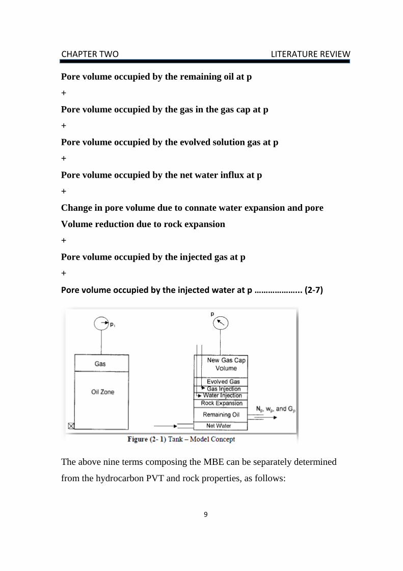
List of Figures Figure (2- 1) Tank – Model Concept .......................................................... 9
Figure (2- 2) Underground withdrawal versus (Eo+Ef,w). ....................... 19
Figure (2- 3) Underground withdrawal (F) versus (Eo). ........................... 20
Figure (2- 4) plot (F / Eo) versus (Eg / Eo) ............................................... 21
Figures (2-5) Production history plot..........................................................25
Figures (2-6) Production history graphs for two really wells.................... 25
Figures (2-7) Cumulative production plot................................................. 26
Figure (2-8) Relationship between production rate and cumulative......... 27
Figure (3- 1) Interface of Petroleum Experiment Package....................... 28
Figure (3-2) Gas-solubility pressure diagram .......................................... 30
Figure (3- 3) Oil formation volume factor ............................................... 38
Figure (3-4) decline curves types ..............................................................46
Figure (3-5) Classification of production decline curves.......................... 47
Figure (3-6) exponential decline curves ................................................... 50
Figure (3-8) Hyperbolic decline curves ................................................... 55
Figure (3-9) decline curve shapes for a Cartesian rate–time plot ............ 58
Figure (3-10) decline curve shapes for a Cartesian cumulative–time……58
Figure (4-1) oil black matching ................................................................ 60
Figure (4-2) Plot of FVF versus Pressure ................................................. 61
IX
Figure (4-3) Plot of Gas Oil Ratio versus pressure ................................... 61
Figure (4-4) Campell – No Aquifer ...........................................................62
Figure (4-5) Graphical Plot (Campbell-aquifer) ....................................... 62
Figure (4- 6) Analytical method after regression .......................................63
Figure (4-7) Energy plot .............................................................................64
Figure (4-8) oil rate and cumulative vs time exponential decline...............65
Figure (4-9) oil rate vs cumulative production exponential decline............65
Figure (4-10) oil rate and cumulative vs time hyperbolic decline ..............67
Figure (4-11) oil rate vs cumulative production hyperbolic decline…........67
Figure (4-12) prediction with water injection (20000 STB/day) ................68
Figure (4- 13) prediction with water injection (40000 STB/day) .............. 69
Figure (4-14) oil rate and cumulative vs time exponential decline…..........71
Figure (4-15) oil rate vs time exponential decline ......................................72
Figure (4-16) oil rate and cumulative vs time exponential decline.............73
Figure (4-17) oil rate vs time exponential decline ......................................74
Figure (4-16) oil rate and cumulative vs time exponential decline.............75
X
NOMENCLATURE
Symbols Description
MBE…………………………………………...Material Balance Equation
DCA……………………………………………...Decline Curve Analysis
Pi…………………………………………......Initial reservoir pressure psi
p…………………………………...Volumetric average reservoir pressure
Δp……………………………...Change in reservoir pressure = pi − p, psi
Pb………………………………………………Bubble point pressure, psi
N…………………...…………………...Initial (original) oil in place, STB
Np…………………………………………Cumulative oil produced, STB
Gp…………………………………………. Cumulative gas produced, scf
Wp………………………………………. Cumulative water produced, bbl
Rp…………………………………........Cumulative gas-oil ratio, scf/STB
GOR…………………………………Instantaneous gas-oil ratio, scf/STB
Rsi…………………………………………. Initial gas solubility, scf/STB
Rs…………………………………………………Gas solubility, scf/STB
Boi…………………….…… Initial oil formation volume factor, bbl/STB
Bo………………………………… Oil formation volume factor, bbl/STB
XI
Bgi…………………………...Initial gas formation volume factor, bbl/scf
Bg…………………………………. Gas formation volume factor, bbl/scf
Winj……………………………………...Cumulative water injected, STB
Ginj……………...…………………………...Cumulative gas injected, scf
We ………………………………………… Cumulative water influx, bbl
G……………………………………………………Initial gas-cap gas, scf
P.V……………………………………………………… Pore volume, bbl
Cw…………………………………………. Water compressibility, psi−1
Cf …………………………….…Formation (rock) compressibility, psi−1
API………………………………………... American Petroleum Institute
T……………………………………………………………... Temperature
d ………………………………………………………… Decline Constant
q………………………………………………………………… Flow Rate
t……………………………………………………………………… Time
K……………………………………………………………… Permeability
µ………………………………………………………………… Viscosity
h………………………………………………………………… thickness
1
CHAPTER ONE INTERODUCTION
CHAPTER_ONE
INTERDUCTION
1-1 Background of the study:
Reservoir engineering is the heart of petroleum engineering. In essence,
reservoir engineering deals with the flow of oil, gas, and water through
porous media in rocks and also with the associated recovery efficiencies.
Reservoir engineers play an active and important role throughout the
reservoir life cycle and in the various phases of the reservoir management
process.
one of the most important job functions as reservoir engineer is the prediction
of future production rates from a given reservoir or specific well. over the
years, engineers have developed several methods to accomplish this task.
In this study we will use two methods, the material balance and decline curve
analysis
1-1-1 Matereal balance
In maternal balance reservoir fluid properties are very important in
computations, these properties are determined from laboratory studies on
samples collected from the bottom of the wellbore or at the surface. Such
experimental solution is to use the empirically derived correlations to predict
PVT properties.
There are many empirical correlations for predicting PVT properties, most of
them were developed using linear or non-linear multiple regression or
graphical techniques. Each correlation was developed for a certain range of
reservoir fluid characteristics and geographical area with similar fluid
2
CHAPTER ONE INTERODUCTION
compositions and API gravity. Thus, the accuracy of such correlations is
critical and it is not often known in advance Among those PVT
properties is the bubble point Oil Formation Volume Factor (Bob), which is
defined as the volume of reservoir oil that would be occupied by one stock
tank barrel oil plus any dissolved gas at the bubble point pressure and
reservoir temperature. Precise prediction of Bob is very important in reservoir
and production computations.
Material balance equation makes use of pressure in the prediction. Tamer and
Muscat method which are widely used do not considered time in their
prediction performance, also neither water influx nor gravity segregation was
considered. Thus, this study incorporates aquifer and time scale to the
equation in making predictions. The time history will be inferred from the
reserves and well production rates, though it does not consider reservoir
geometry, Heterogeneity, fluid distribution, the drainage area, the position
and orientation of the wells.
1-1-2 Decline curve analysis
Decline curve analysis is a graphical procedure used for analyzing
declining production rates and forecasting future performance of oil and gas
wells. A curve fit of past production performance is done using certain
standard curves. This curve fit is then extrapolated to predict potential future
performance. Decline curve analysis is a basic tool for estimating recoverable
reserves. Conventional or basic decline curve analysis can be used only when
the production history is long enough that a trend can be identified.
3
CHAPTER ONE INTERODUCTION
Decline curve analysis is not grounded in fundamental theory but is
based on empirical observations of production decline. Three types of decline
curves have been identified; exponential, hyperbolic, and harmonic.
exponential decline predicts a faster decline than hyperbolic or harmonic. As
a result, it is often used to calculate the minimum "proved reserves" while
hyperbolic decline predicts a slower decline rate than exponential. As a
result, it is sometimes used to calculate the "probable reserves".
Well production drops rather slowly with time under harmonic decline, in
comparison to exponential or hyperbolic decline, given that all other
parameters are the same. Consequently, harmonic decline indicates relatively
large reserves. Two sets of curves are normally used while analyzing
production decline. Flow rate is plotted against Time and Flow rate against
cumulative production. Time is the most convenient independent variable
because extrapolation of rate-time graphs can be directly used for production
forecasting and economic evaluations.
However, plots of rate vs. cumulative production have their own advantages;
Not only do they provide a direct estimate of the ultimate recovery at a
specified economic limit, but will also yield a more rigorous interpretation in
situations where the production is influenced by intermittent operations.
This Study used (MBAL) software to predict the future performance of the
reservoir in both methods material balance and decline curve analysis.
4
CHAPTER ONE INTERODUCTION
1-2 objectives of the study
1-To estimate of initial oil in place by using material balance method
2- To estimate of remains recoverable hydrocarbons, proved reserves and
probable reserves by using decline curve method.
3- Determine the type of the drive mechanism in the system.
4- To know the performance of the well or groups of wells in the reservoir
and prediction of the flow rate in the future.
5- suggestion the methods that enhanced oil recovery in high efficient to
recover the same reserve in less time.

5
CHAPTER TWO LITERATURE REVIEW
CHAPTER TWO
Literature Review
Material balance 1-2
Tarek (2010) stated that material balance equation, (MBE) plays a major role
in most reservoir engineering calculations. It helps reservoir engineers to
constantly seek for ways to optimize hydrocarbon recovery by predicting the
future performance of the reservoir. We should note that the (MBE) simply
provides performance as a function of average reservoir pressure without the
fluid flow concepts. Combining the (MBE) and fluid flow concepts would
enable the engineer to predict the reservoir future production performance as
a function of time. Odeh & Havlena (1963) rearrange (MBE) into different
linear forms. This method requires the plotting of a variable group against
another variable group selected depending on the reservoir drive mechanism
and if linear relationship does not exist, then this deviation suggests that
reservoir is not performing as anticipated and other mechanisms are involved
which were not accounted for but once linearity has been achieved, based on
matching pressure and production data then a mathematical model has been
achieved. This technique is referred to as history matching. Therefore, the
application of the model enables predictions of the future reservoir
performance. There are several methods which have appeared in literatures
for predicting the performance solution gas behavior relating pressure decline
to gas-oil ratio and oil recovery. Tamer (1944) and Muskat (1945) proposed
an iterative technique to predict the performance of depletion (solution-gas)
- drive reservoirs under internal gas drive mechanism, using rock and fluid
properties. The assumptions of both methods include negligible gravity
6
CHAPTER TWO LITERATURE REVIEW
segregation forces. These authors considered only thin, horizontal reservoirs.
Both methods use the material balance principle (static) and a producing gas-
oil ratio equation (dynamic) to predict reservoir performance at pressures. A
more detailed description of both methods appears in Craft and Hawkins
Tracy (1955) in the model developed for reservoir performance prediction,
did not consider oil reservoirs above the bubble-point pressure (under
saturated reservoir). It is normally started at the bubble-point pressure or at
pressures below. To use this method for predicting future performance, it is
necessary to choose the future pressures at which performance is desired.
This means that we need to select the pressure step to be used. Furthermore,
among these methods of reservoir performance prediction, none considered
aquifer in the (MBE) hence, the software developed for this study
incorporated aquifer into Tamer's method of reservoir performance
prediction for solution gas drive. Three aquifer models such as Hurst Van
Everdingen (1947), Carter-Tracy (1960) and Fetkovich (1971) were
programmed to allow for flexibility Classic analytical models of aquifers are
relatively easy to program in computer spreadsheets, provided that equation
discretization is correctly done. With the exception of the van Everdingen &
Hurst, the models do not demand much computer power. In the van
Everdingen & Hurst, calculations of the previous steps are redone at each
time step added to the behavior, which represents a bigger computational
effort. The equation that rules the van Everdingen & Hurst model is based on
the superposition principle. Any numerical calculation method for this model
requires more computing power than other models. Despite this drawback, it
is the ideal model for comparisons, because it faithfully represents the
hydraulic diffusivity equation. Other proposed models, such as Carter &
Tracy, Fetkovich and Leung, sought t eliminate the disadvantage of the
7
CHAPTER TWO LITERATURE REVIEW
required computing power and thus became more popular in commercial
flow simulators. The error of this model in computing the accumulated influx
is insignificant when compared to the base model (van Everdingen & Hurst).
2.1.1 Material Balance Theory:
Schillthuis (1936) first presented a method of reservoir estimation using the
material balance. Material balance is a volumetric balance which states that
since the volume of a reservoir (as defined by its initial limits) is constant,
the cumulative observed production, expressed as an underground
withdrawal, must equal the expansion of fluids in the reservoir resulting from
finite pressure drop.
2.1.2 Derivative of Material Balance Equation:
The equation is structured to simply keep inventory of all materials entering,
leaving and accumulating in the reservoir. The concept of the material
balance equation was presented by Schilthuis in (1941). In its simplest form,
the equation can be written on volumetric basis as:
Initial volume = volume remaining + volume removed ……...…. (2-1)
Since oil, gas and water are present in petroleum reservoirs, the material
balance equation can be expressed for the total fluids or for any one of the
fluids present. Before deriving the material balance, it is convenient to denote
certain terms by symbols for brevity. The symbols used conform where
possible to the standard nomenclature adopted by the Society of Petroleum
Engineers.
Several of the material balance calculations require the total pore volume
(P.V) as expressed in terms of the initial oil volume N and the volume of the
gas cap. The expression for the total pore volume can be Oil Recovery
8
CHAPTER TWO LITERATURE REVIEW
Mechanisms and the Material Balance Equation derived by conveniently
introducing the parameter m into the relationship as follows:
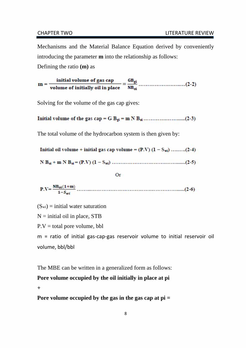
Defining the ratio (m) as
Solving for the volume of the gas cap gives:
The total volume of the hydrocarbon system is then given by:
(Swi) = initial water saturation
N = initial oil in place, STB
P.V = total pore volume, bbl
m = ratio of initial gas-cap-gas reservoir volume to initial reservoir oil
volume, bbl/bbl
The MBE can be written in a generalized form as follows:
Pore volume occupied by the oil initially in place at pi
+
Pore volume occupied by the gas in the gas cap at pi =
9
CHAPTER TWO LITERATURE REVIEW
Pore volume occupied by the remaining oil at p
+
Pore volume occupied by the gas in the gas cap at p
+
Pore volume occupied by the evolved solution gas at p
+
Pore volume occupied by the net water influx at p
+
Change in pore volume due to connate water expansion and pore
Volume reduction due to rock expansion
+
Pore volume occupied by the injected gas at p
+
Pore volume occupied by the injected water at p ………………... (2-7)
The above nine terms composing the MBE can be separately determined
:from the hydrocarbon PVT and rock properties, as follows
10
CHAPTER TWO LITERATURE REVIEW
:Pore Volume Occupied by the Oil Initially in Place
Volume occupied by initial oil in place = N Boi …………….… (2-8) Where:
N = oil initially in place, STB
Boi = oil formation volume factor at initial reservoir pressure (pi), bbl/STB
Pore Volume Occupied by the Gas in the Gas Cap:
Volume of gas cap = m N Boi ……………………………………... (2-9)
Where:
m: is a dimensionless parameter and defined as the ratio of gas-cap volume
to the oil zone volume.
Pore Volume Occupied by the Remaining Oil:
Volume of the remaining oil = (N − Np) ……………………....… (2-10)
Where:
Np = cumulative oil production, STB
Bo = oil formation volume factor at reservoir pressure p, bbl/STB
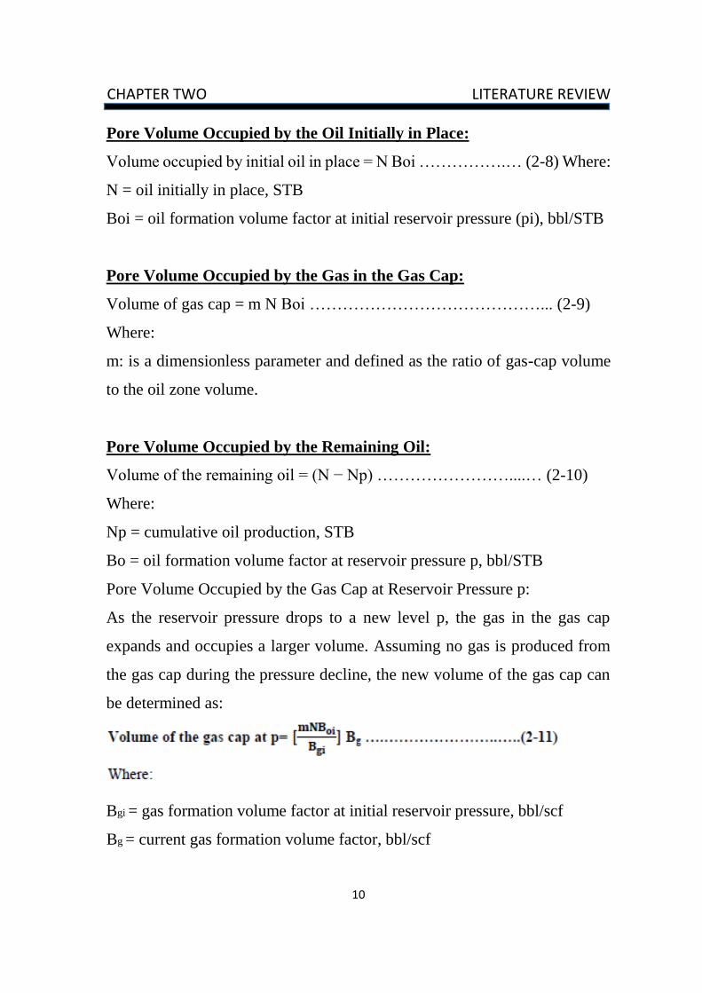
Pore Volume Occupied by the Gas Cap at Reservoir Pressure p:
As the reservoir pressure drops to a new level p, the gas in the gas cap
expands and occupies a larger volume. Assuming no gas is produced from
the gas cap during the pressure decline, the new volume of the gas cap can
be determined as:
Bgi = gas formation volume factor at initial reservoir pressure, bbl/scf
Bg = current gas formation volume factor, bbl/scf
11
CHAPTER TWO LITERATURE REVIEW
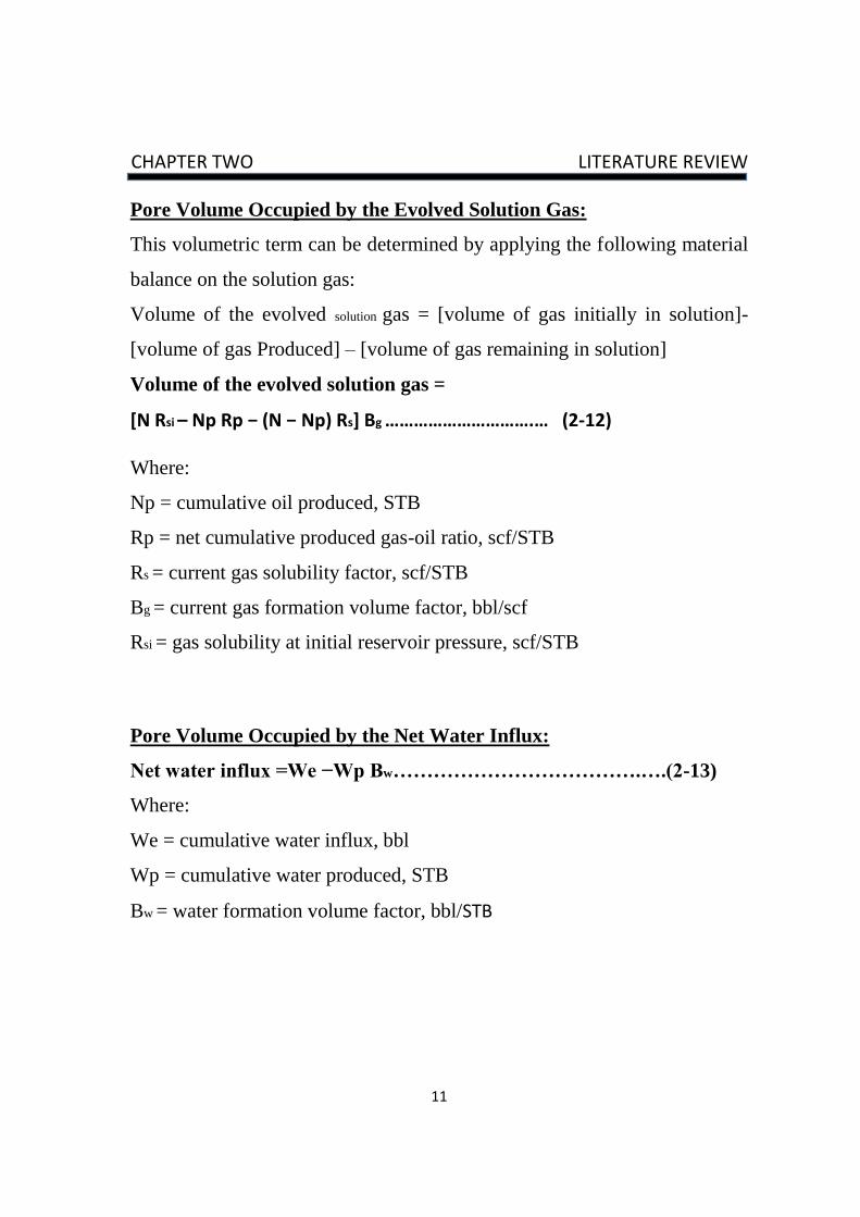
Pore Volume Occupied by the Evolved Solution Gas:
This volumetric term can be determined by applying the following material
balance on the solution gas:
Volume of the evolved solution gas = [volume of gas initially in solution]-
[volume of gas Produced] – [volume of gas remaining in solution]
Volume of the evolved solution gas =
[N Rsi – Np Rp − (N − Np) Rs] Bg ………………………….… (2-12)
Where:
Np = cumulative oil produced, STB
Rp = net cumulative produced gas-oil ratio, scf/STB
Rs = current gas solubility factor, scf/STB
Bg = current gas formation volume factor, bbl/scf
Rsi = gas solubility at initial reservoir pressure, scf/STB
Pore Volume Occupied by the Net Water Influx:
Net water influx =We −Wp Bw……………………………….….(2-13)
Where:
We = cumulative water influx, bbl
Wp = cumulative water produced, STB
Bw = water formation volume factor, bbl/STB
12
CHAPTER TWO LITERATURE REVIEW
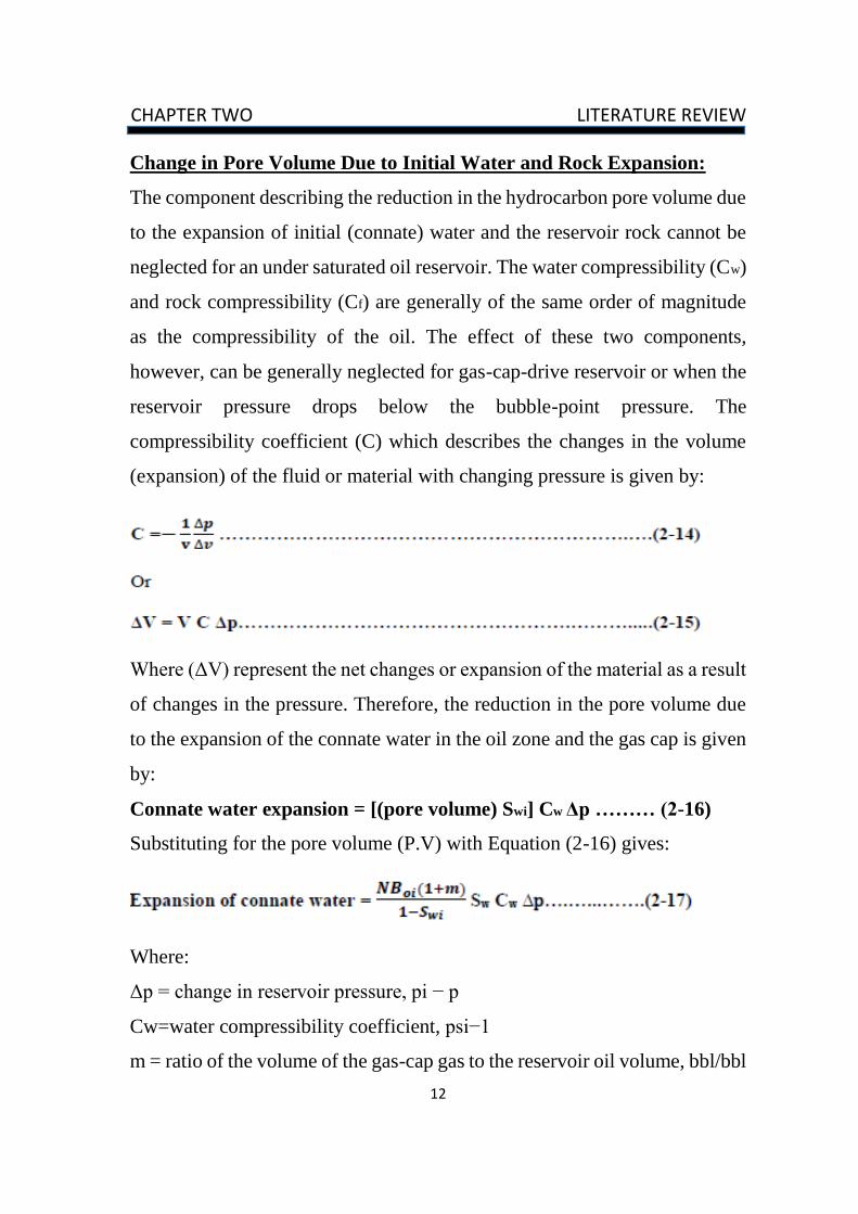
Change in Pore Volume Due to Initial Water and Rock Expansion:
The component describing the reduction in the hydrocarbon pore volume due
to the expansion of initial (connate) water and the reservoir rock cannot be
neglected for an under saturated oil reservoir. The water compressibility (Cw)
and rock compressibility (Cf) are generally of the same order of magnitude
as the compressibility of the oil. The effect of these two components,
however, can be generally neglected for gas-cap-drive reservoir or when the
reservoir pressure drops below the bubble-point pressure. The
compressibility coefficient (C) which describes the changes in the volume
(expansion) of the fluid or material with changing pressure is given by:
Where (ΔV) represent the net changes or expansion of the material as a result
of changes in the pressure. Therefore, the reduction in the pore volume due
to the expansion of the connate water in the oil zone and the gas cap is given
by:
Connate water expansion = [(pore volume) Swi] Cw Δp ……… (2-16)
Substituting for the pore volume (P.V) with Equation (2-16) gives:
Where:
Δp = change in reservoir pressure, pi − p
Cw=water compressibility coefficient, psi−1
m = ratio of the volume of the gas-cap gas to the reservoir oil volume, bbl/bbl
13
CHAPTER TWO LITERATURE REVIEW
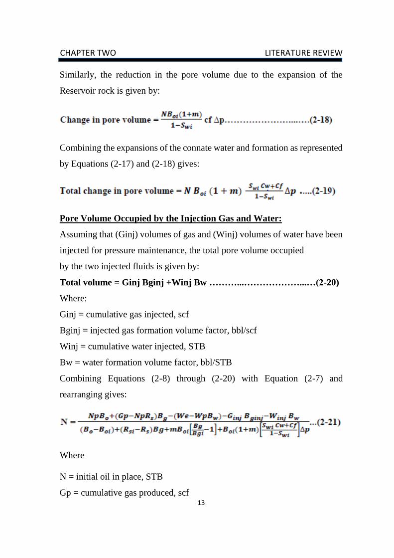
Similarly, the reduction in the pore volume due to the expansion of the
Reservoir rock is given by:
Combining the expansions of the connate water and formation as represented
by Equations (2-17) and (2-18) gives:
Pore Volume Occupied by the Injection Gas and Water:
Assuming that (Ginj) volumes of gas and (Winj) volumes of water have been
injected for pressure maintenance, the total pore volume occupied
by the two injected fluids is given by:
Total volume = Ginj Bginj +Winj Bw ………...………………...…(2-20)
Where:
Ginj = cumulative gas injected, scf
Bginj = injected gas formation volume factor, bbl/scf
Winj = cumulative water injected, STB
Bw = water formation volume factor, bbl/STB
Combining Equations (2-8) through (2-20) with Equation (2-7) and
rearranging gives:
Where
N = initial oil in place, STB
Gp = cumulative gas produced, scf
14
CHAPTER TWO LITERATURE REVIEW
Np = cumulative oil produced, STB
Rsi = gas solubility at initial pressure, scf/STB
m = ratio of gas-cap gas volume to oil volume, bbl/bbl
Bgi = gas formation volume factor at pi, bbl/scf
Bginj = gas formation volume factor of the injected gas, bbl/scf
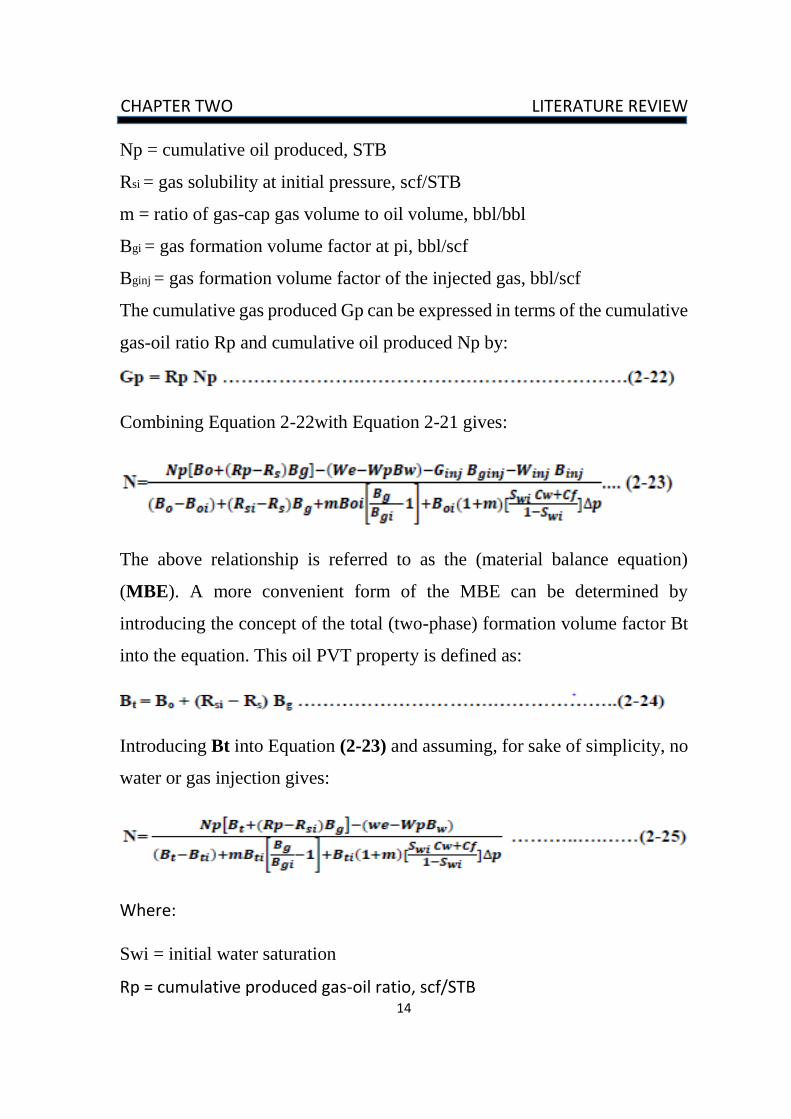
The cumulative gas produced Gp can be expressed in terms of the cumulative
gas-oil ratio Rp and cumulative oil produced Np by:
Combining Equation 2-22with Equation 2-21 gives:
The above relationship is referred to as the (material balance equation)
(MBE). A more convenient form of the MBE can be determined by
introducing the concept of the total (two-phase) formation volume factor Bt
into the equation. This oil PVT property is defined as:
Introducing Bt into Equation (2-23) and assuming, for sake of simplicity, no
water or gas injection gives:
Where:
Swi = initial water saturation
Rp = cumulative produced gas-oil ratio, scf/STB
15
CHAPTER TWO LITERATURE REVIEW
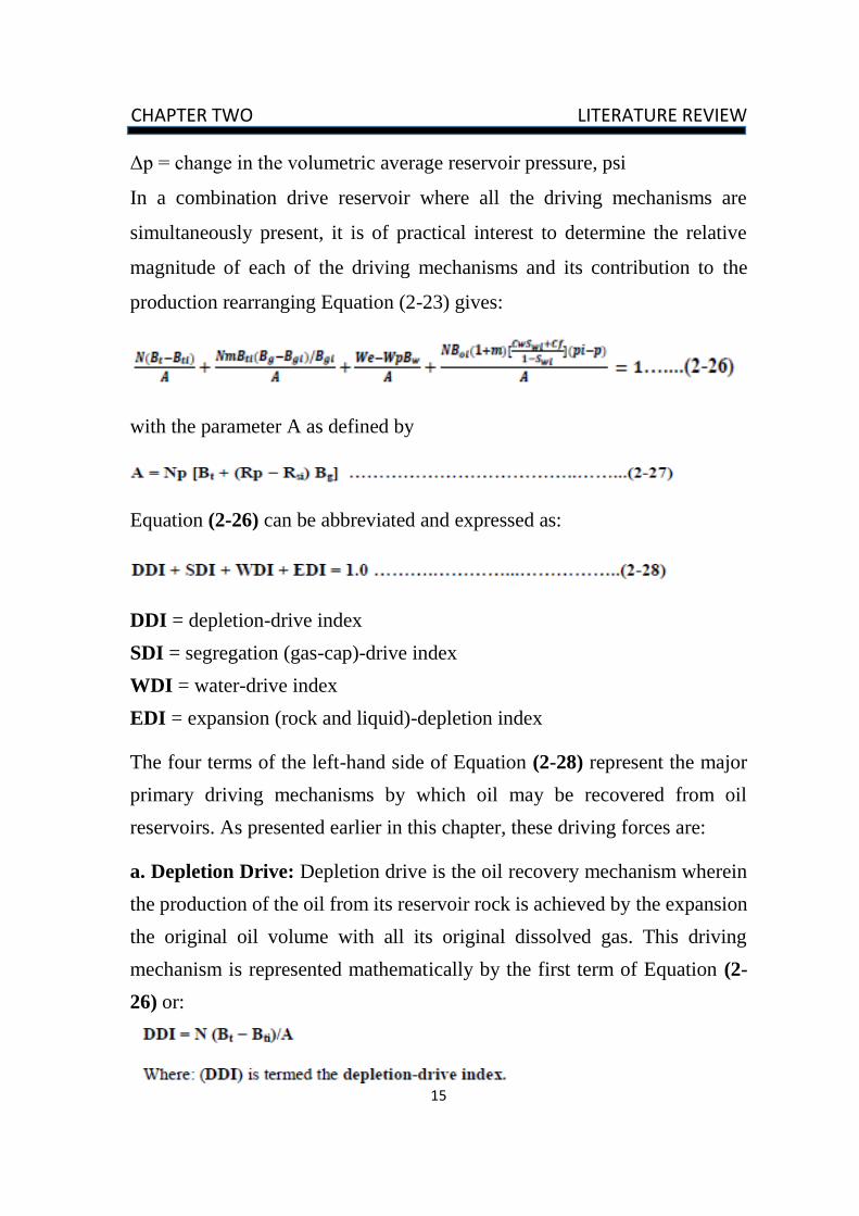
Δp = change in the volumetric average reservoir pressure, psi
In a combination drive reservoir where all the driving mechanisms are
simultaneously present, it is of practical interest to determine the relative
magnitude of each of the driving mechanisms and its contribution to the
production rearranging Equation (2-23) gives:
with the parameter A as defined by
Equation (2-26) can be abbreviated and expressed as:
DDI = depletion-drive index
SDI = segregation (gas-cap)-drive index
WDI = water-drive index
EDI = expansion (rock and liquid)-depletion index
The four terms of the left-hand side of Equation (2-28) represent the major
primary driving mechanisms by which oil may be recovered from oil
reservoirs. As presented earlier in this chapter, these driving forces are:
a. Depletion Drive: Depletion drive is the oil recovery mechanism wherein
the production of the oil from its reservoir rock is achieved by the expansion
the original oil volume with all its original dissolved gas. This driving
mechanism is represented mathematically by the first term of Equation (2-
26) or:
16
CHAPTER TWO LITERATURE REVIEW
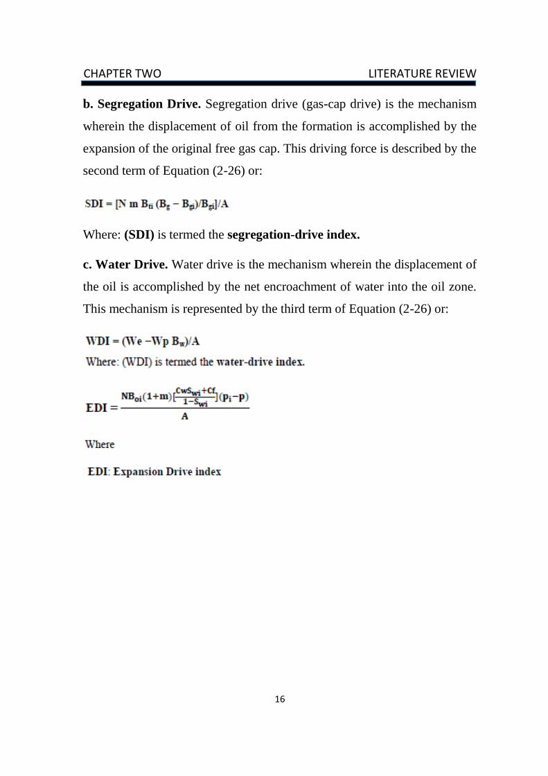
b. Segregation Drive. Segregation drive (gas-cap drive) is the mechanism
wherein the displacement of oil from the formation is accomplished by the
expansion of the original free gas cap. This driving force is described by the
second term of Equation (2-26) or:
Where: (SDI) is termed the segregation-drive index.
c. Water Drive. Water drive is the mechanism wherein the displacement of
the oil is accomplished by the net encroachment of water into the oil zone.
This mechanism is represented by the third term of Equation (2-26) or:
17
CHAPTER TWO LITERATURE REVIEW
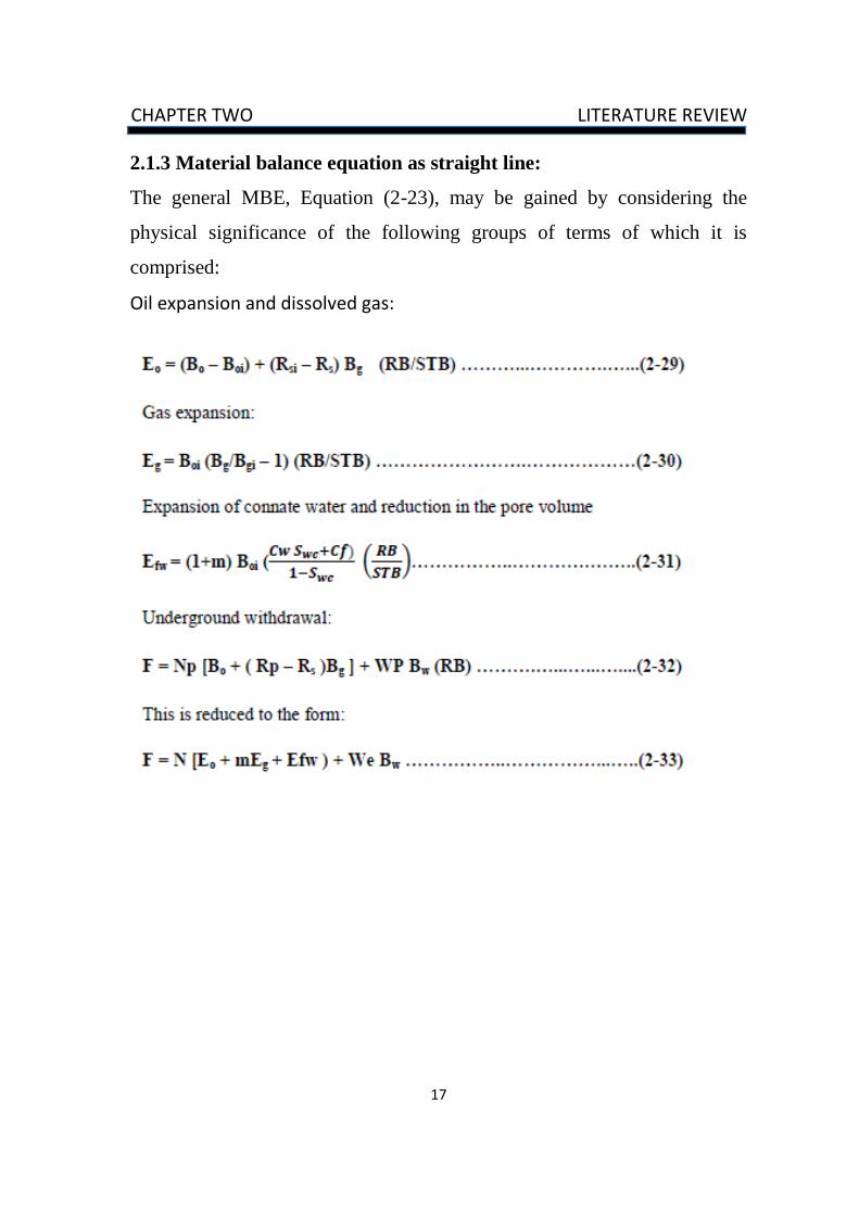
2.1.3 Material balance equation as straight line:
The general MBE, Equation (2-23), may be gained by considering the
physical significance of the following groups of terms of which it is
comprised:
Oil expansion and dissolved gas:
18
CHAPTER TWO LITERATURE REVIEW
2-1-4 The Straight-Line Solution Method To The MBE:
The straight-line solution method requires the plotting of a variable group
versus another variable group, with the variable group selection depending
on the mechanism of production under which the reservoir is producing. The
most important aspect of this method of solution is that it attaches
significance the sequence of the plotted points, the direction in which they
plot, and to the shape of the resulting plot. The significance of the straight-
line approach is that the sequence of plotting is important and if the plotted
data deviates from this straight line there is some reason for it. This
significant observation will provide the engineer with valuable information
that can be used in determining the following unknowns:
- Initial oil in place N
- Size of the gas cap m
- Water influx We.
- Driving mechanism
The remainder of this chapter is devoted to illustrations of the use of the
straight-line solution method in determining N, m, and We for different
reservoir mechanisms.
Case1. Volumetric Under saturated-Oil Reservoirs
Assuming no water or gas injection, the linear form of the MBE as expressed
by Equation (2-23) can be written as:
F = N [Eo + m Eg + Ef,w] +We ………………………...………...…(2-34)
Several terms in the above relationship may disappear when imposing the
conditions associated with the assumed reservoir driving mechanism. For
a volumetric and under saturated reservoir, the conditions associated with
driving mechanism are:
19
CHAPTER TWO LITERATURE REVIEW
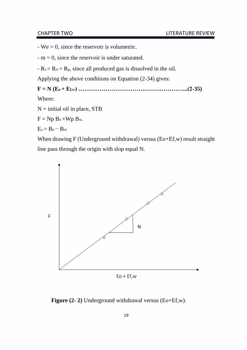
- We = 0, since the reservoir is volumetric.
- m = 0, since the reservoir is under saturated.
- Rs = Rsi = Rp, since all produced gas is dissolved in the oil.
Applying the above conditions on Equation (2-34) gives:
F = N (Eo + Ef,w) ………………………………………………...(2-35)
Where:
N = initial oil in place, STB
F = Np Bo +Wp Bw.
Eo = Bo − Boi
When drawing F (Underground withdrawal) versus (Eo+Ef,w) result straight
line pass through the origin with slop equal N.
Figure (2- 2) Underground withdrawal versus (Eo+Ef,w).
20
CHAPTER TWO LITERATURE REVIEW
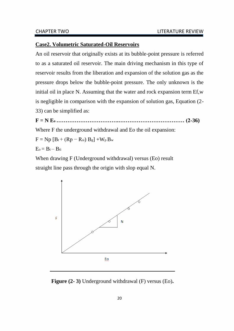
Case2. Volumetric Saturated-Oil Reservoirs
An oil reservoir that originally exists at its bubble-point pressure is referred
to as a saturated oil reservoir. The main driving mechanism in this type of
reservoir results from the liberation and expansion of the solution gas as the
pressure drops below the bubble-point pressure. The only unknown is the
initial oil in place N. Assuming that the water and rock expansion term Ef,w
is negligible in comparison with the expansion of solution gas, Equation (2-
33) can be simplified as:
F = N Eo …………………………….……………………………… (2-36)
Where F the underground withdrawal and Eo the oil expansion:
F = Np [Bt + (Rp − Rsi) Bg] +Wp Bw
Eo = Bt – Bti
When drawing F (Underground withdrawal) versus (Eo) result
straight line pass through the origin with slop equal N.
Figure (2- 3) Underground withdrawal (F) versus (Eo).
21
CHAPTER TWO LITERATURE REVIEW
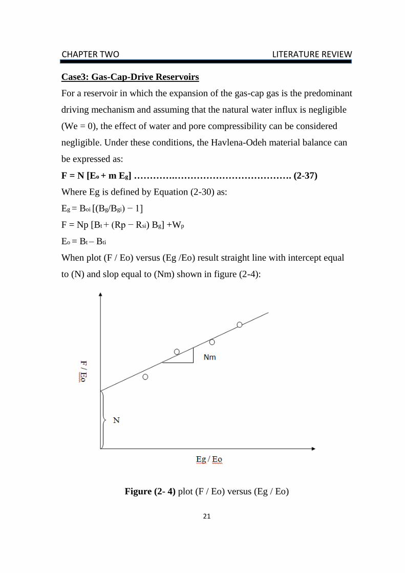
Case3: Gas-Cap-Drive Reservoirs
For a reservoir in which the expansion of the gas-cap gas is the predominant
driving mechanism and assuming that the natural water influx is negligible
(We = 0), the effect of water and pore compressibility can be considered
negligible. Under these conditions, the Havlena-Odeh material balance can
be expressed as:
F = N [Eo + m Eg] ………….………………………………. (2-37)
Where Eg is defined by Equation (2-30) as:
Eg = Boi [(Bg/Bgi) − 1]
F = Np [Bt + (Rp − Rsi) Bg] +Wp
Eo = Bt – Bti
When plot (F / Eo) versus (Eg /Eo) result straight line with intercept equal
to (N) and slop equal to (Nm) shown in figure (2-4):
Figure (2- 4) plot (F / Eo) versus (Eg / Eo)
22
CHAPTER TWO LITERATURE REVIEW
curve Decline 2-2
I koku (1984) presented a comprehensive and rigorous treatment of
production-decline-curve analysis. He pointed out that the following three
conditions must be considered in production-decline-curve analysis:
,
1. Certain conditions must prevail before we can analyze a production decline
curve with any degree of reliability. The production must have been stable
over the period being analyzed; that is, a flowing well must have been
produced with constant choke size or constant wellhead pressure and a
pumping well must have been pumped off or produced with constant fluid
level. These indicate that the well must have been produced at capacity under
a given set of conditions. The production decline observed should truly effect
reservoir productivity and not be the result of an external cause, such as a
change in production conditions, Well damage, production controls, or
equipment failure.
2. Stable reservoir conditions must also prevail in order to extrapolate decline
curves with any degree of reliability. This condition will normally be met as
long as the producing mechanism is not altered. However, when an action is
taken to improve the recovery of gas, such an infill drilling, fluid injection,
fracturing, or acidizing, decline-curve analysis can be used to estimate the
performance of the well or reservoir in the absence of the change and
compare it to the actual performance with the change. This comparison will
enable us to determine the technical and economic success of our efforts
3. Production-decline-curve analysis is used in the evaluation of new
investments and the audit of previous expenditures. Associated with this is
the sizing of equipment and facilities such as pipelines, plants, and treating
23
CHAPTER TWO LITERATURE REVIEW
facilities. Also associated with the economic analysis is the determination of
reserves for a well, lease, or field. This is an independent method of reserve
estimation, the result of which can be compared to volumetric or material-
balance estimates
2-2-1 Golden rule of DCA
The basic assumption in this procedure is that whatever causes
controlled the trend of a curve in the past will continue to govern its trend in
the future in a uniform manner.
2-2-2 History of DCA
J.J. Arps collected these ideas into a comprehensive set of equations
defining the exponential, hyperbolic and harmonic declines. His work was
further extended by other researchers to include special
cases. Following section gives a historical perspective of work done on the
subject;
Arps 1945 and 1956.
Browns 1963 and Fetkovitch 1983 applied constant pressure solution to
diffusivity equation and demonstrated that exponential decline curve
actually reflects single phase, incompressible fluid production from a
closed reservoir. DCA is more than a empirical curve fit.
Fetkovitch 1980 and 1983 developed set of type curves to enhance
application of DCA.
Doublet and Blasingame 1995 developed theoretical basis for combining
transient and boundary dominated flow for the pressure transient solution
to the diffusivity equation
24
CHAPTER TWO LITERATURE REVIEW
2-2-3 DCA in Today
The major application of DCA in the industry today is still based on
equations and curves described by Arps. Arps applied the equation of
Hyperbola to define three general equations to model production declines.
In order to locate a hyperbola in space one must know the following three
variables.
1. The starting point on Y axis, (qi), initial rate.
2. Initial decline rate (Di)
3. The degree of curvature of the line (b).
Arps did not provide physical reasons for the three types of decline. He
only indicated that exponential decline (b=0) is most common and that the
coefficient b generally ranges from 0 to 0.5.
Arp’s Equation for General Decline in a Well ..........................(1)
Clearly all wells do not exhibit exponential behavior during depletion.
In many cases a more gradual hyperbolic decline is observed where rate time
performance is better than estimated from exponential solutions implying
that hyperbolic decline results from natural and artificial driving energies that
slow down pressure depletion. Hyperbolic decline is observed when reservoir
drive mechanism is solution gas cap drive, gas cap expansion or water drive.
It is also possible where natural drive is supplemented by injection of water
gas. The type of decline and its characteristic shape is a major feature of
25
CHAPTER TWO LITERATURE REVIEW
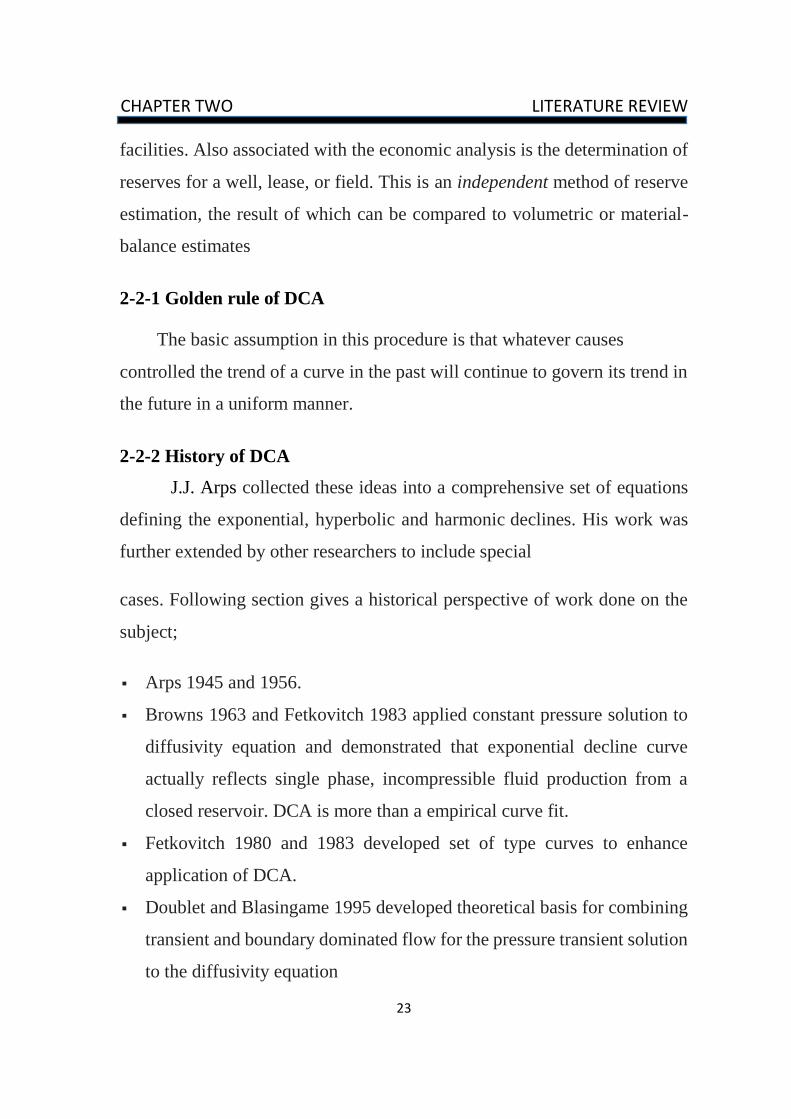
DCA. We shall be talking more about this as we go further. The various types
of declines experienced by a well are documented in the Fig (2-1a) and Fig(2-
1b) INSERT FIGURE 1 q vs.
Time showing various types of declines on Cartesian plot. (b value for
hyperbolic curve =0.5) (Pending permission approval) INSERT FIGURE 2
Log q vs. Time showing various types of declines on Semi log plot. (b value
for hyperbolic curve =0.5). Note change in shapes of curves. (Pending
permission approval)
Figures (2-5) Production history plot: linear (Cartesian coordinate (left),
semi-logarithmic plot (right)
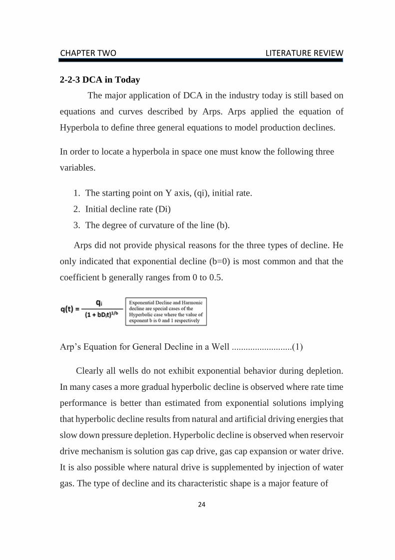
figures (2-6) Production history graphs for two really wells: linear scale
(left), semi-log scale (right)
26
CHAPTER TWO LITERATURE REVIEW
Observe the change in Shapes of curve from Cartesian to logarithmic;
this is very helpful in identification of type of decline.
Two sets of curves are normally used while analyzing production decline.
1. Flow rate is plotted against Time:
a. Very convenient since it provides future profiles directly.
2. Flow rate against cumulative production:
a. Able to incorporate impact of intermittent operations that impact
production.
b. Provide recovery estimates at a specific economic limit.
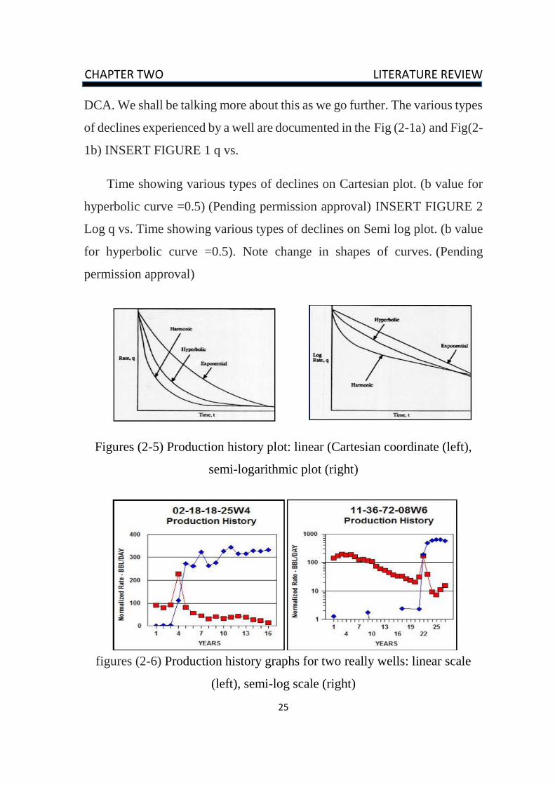
Virtually all oil and gas wells produce at a declining rate over time. The
initial flow rate may be held constant on purpose (restricted rate) or the
decline may begin immediately. The ultimate recovery from the well
(reserves) can be calculated by projecting the decline rate forward in time to
an economic limit. The projected production can be summed to find the total
production on decline, and this can be added to the production during the
constant rate period to obtain the ultimate recovery.
Figures (2-7) Cumulative production plot: linear (Cartesian coordinate
(left), semi- logarithmic plot (right).
27
CHAPTER TWO LITERATURE REVIEW
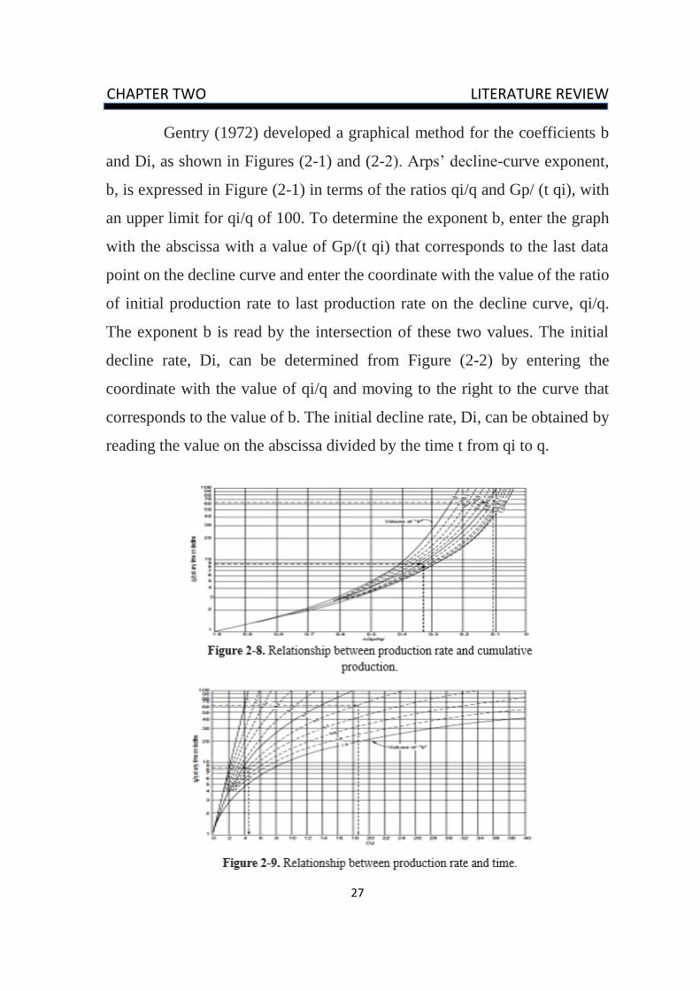
Gentry (1972) developed a graphical method for the coefficients b
and Di, as shown in Figures (2-1) and (2-2). Arps’ decline-curve exponent,
b, is expressed in Figure (2-1) in terms of the ratios qi/q and Gp/ (t qi), with
an upper limit for qi/q of 100. To determine the exponent b, enter the graph
with the abscissa with a value of Gp/(t qi) that corresponds to the last data
point on the decline curve and enter the coordinate with the value of the ratio
of initial production rate to last production rate on the decline curve, qi/q.
The exponent b is read by the intersection of these two values. The initial
decline rate, Di, can be determined from Figure (2-2) by entering the
coordinate with the value of qi/q and moving to the right to the curve that
corresponds to the value of b. The initial decline rate, Di, can be obtained by
reading the value on the abscissa divided by the time t from qi to q.
28
CHAPTER THREE METHODOLOGY
CHAPTER THREE
METHODOLOGY
3-1 The Software (The M-BALTM 10.5) Used For the Study:
M-BALTM 10.5 software package developed by Petroleum Experts was
used as a material balance and decline curve analysis for this evaluation.
M-BALTM is a software application made up of various tools designed to
help the reservoir engineer gain a better understanding of the reservoir
behavior.
Figure (3- 1) Interface of Petroleum Experiment Package
29
CHAPTER THREE METHODOLOGY
3-2 Material balance
3-2-1 Theory of Correlations:
3-2-1-1 Gas Solubility:
The gas solubility Rs is defined as the number of standard cubic feet of gas
which will dissolve in one stock-tank barrel of crude oil at certain pressure
and temperature. The solubility of a natural gas in a crude oil is a strong
function of the pressure, temperature, API gravity, and gas gravity.
For a particular gas and crude oil to exist at a constant temperature, the
solubility increases with pressure until the saturation pressure is reached. At
the saturation pressure all the available gases are dissolved in the oil and the
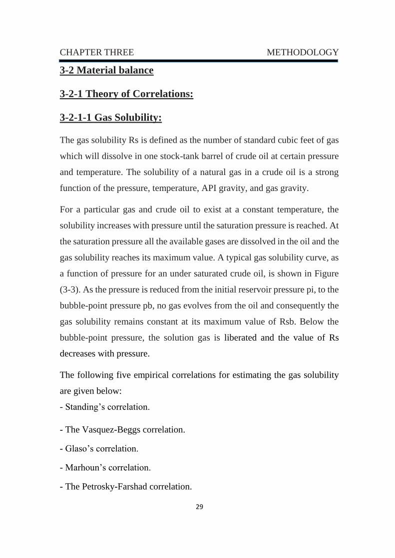
gas solubility reaches its maximum value. A typical gas solubility curve, as
a function of pressure for an under saturated crude oil, is shown in Figure
(3-3). As the pressure is reduced from the initial reservoir pressure pi, to the
bubble-point pressure pb, no gas evolves from the oil and consequently the
gas solubility remains constant at its maximum value of Rsb. Below the
bubble-point pressure, the solution gas is liberated and the value of Rs
decreases with pressure.
The following five empirical correlations for estimating the gas solubility
are given below:
- Standing’s correlation.
- The Vasquez-Beggs correlation.
- Glaso’s correlation.
- Marhoun’s correlation.
- The Petrosky-Farshad correlation.
30
CHAPTER THREE METHODOLOGY
Figure (3-2) Gas-solubility pressure diagram
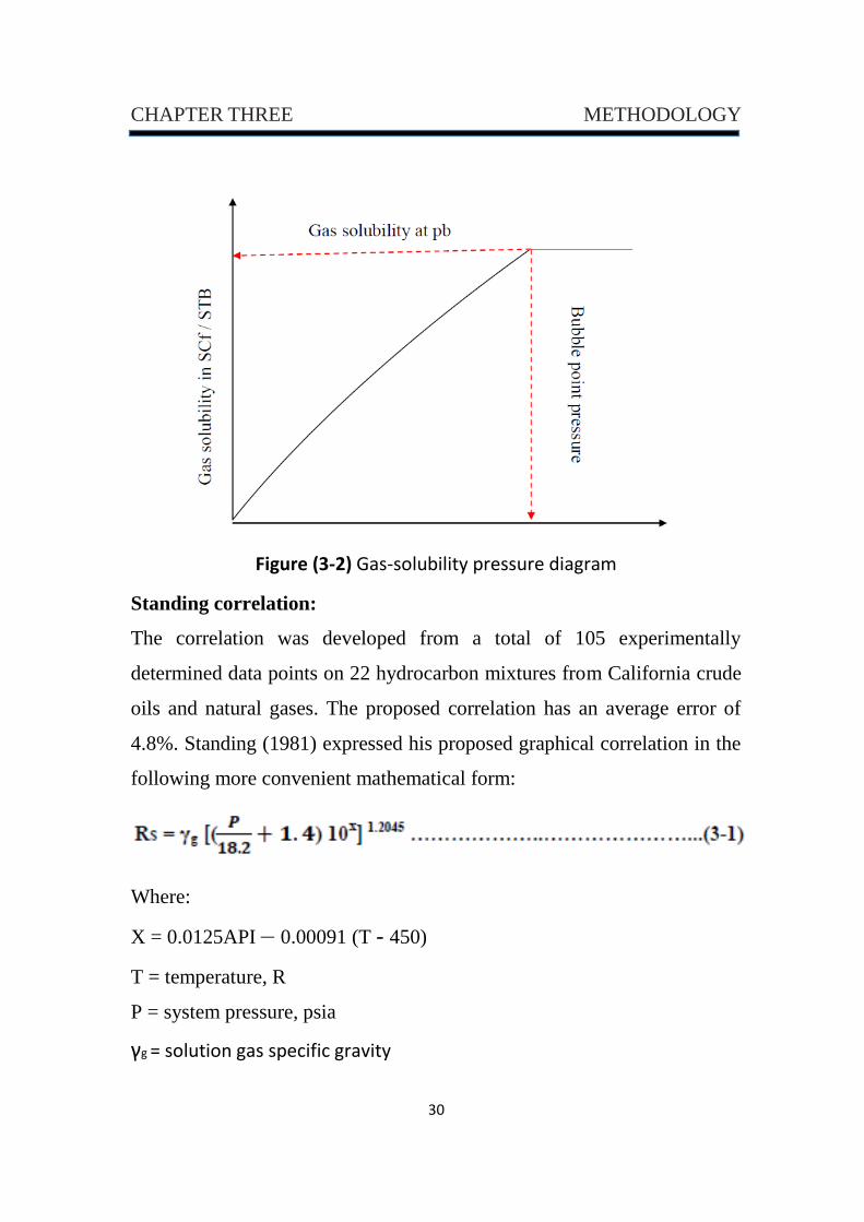
Standing correlation:
The correlation was developed from a total of 105 experimentally
determined data points on 22 hydrocarbon mixtures from California crude
oils and natural gases. The proposed correlation has an average error of
4.8%. Standing (1981) expressed his proposed graphical correlation in the
following more convenient mathematical form:
Where:
X = 0.0125API – 0.00091 (T - 450)
T = temperature, R
P = system pressure, psia
γg = solution gas specific gravity
31
CHAPTER THREE METHODOLOGY
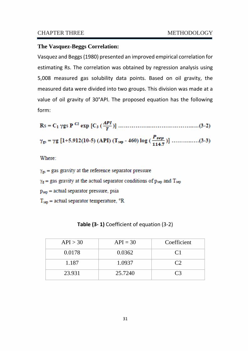
The Vasquez-Beggs Correlation:
Vasquez and Beggs (1980) presented an improved empirical correlation for
estimating Rs. The correlation was obtained by regression analysis using
5,008 measured gas solubility data points. Based on oil gravity, the
measured data were divided into two groups. This division was made at a
value of oil gravity of 30°API. The proposed equation has the following
form:
Table (3- 1) Coefficient of equation (3-2)
Coefficient API = 30 API > 30
C1 0.0362 0.0178
C2 1.0937 1.187
C3 25.7240 23.931
32
CHAPTER THREE METHODOLOGY
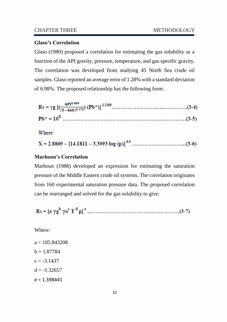
Glaso’s Correlation
Glaso (1980) proposed a correlation for estimating the gas solubility as a
function of the API gravity, pressure, temperature, and gas specific gravity.
The correlation was developed from studying 45 North Sea crude oil
samples. Glaso reported an average error of 1.28% with a standard deviation
of 6.98%. The proposed relationship has the following form:
Marhoun’s Correlation
Marhoun (1988) developed an expression for estimating the saturation
pressure of the Middle Eastern crude oil systems. The correlation originates
from 160 experimental saturation pressure data. The proposed correlation
can be rearranged and solved for the gas solubility to give:
Where:
a = 185.843208
b = 1.87784
c = -3.1437
d = -1.32657
e = 1.398441
33
CHAPTER THREE METHODOLOGY
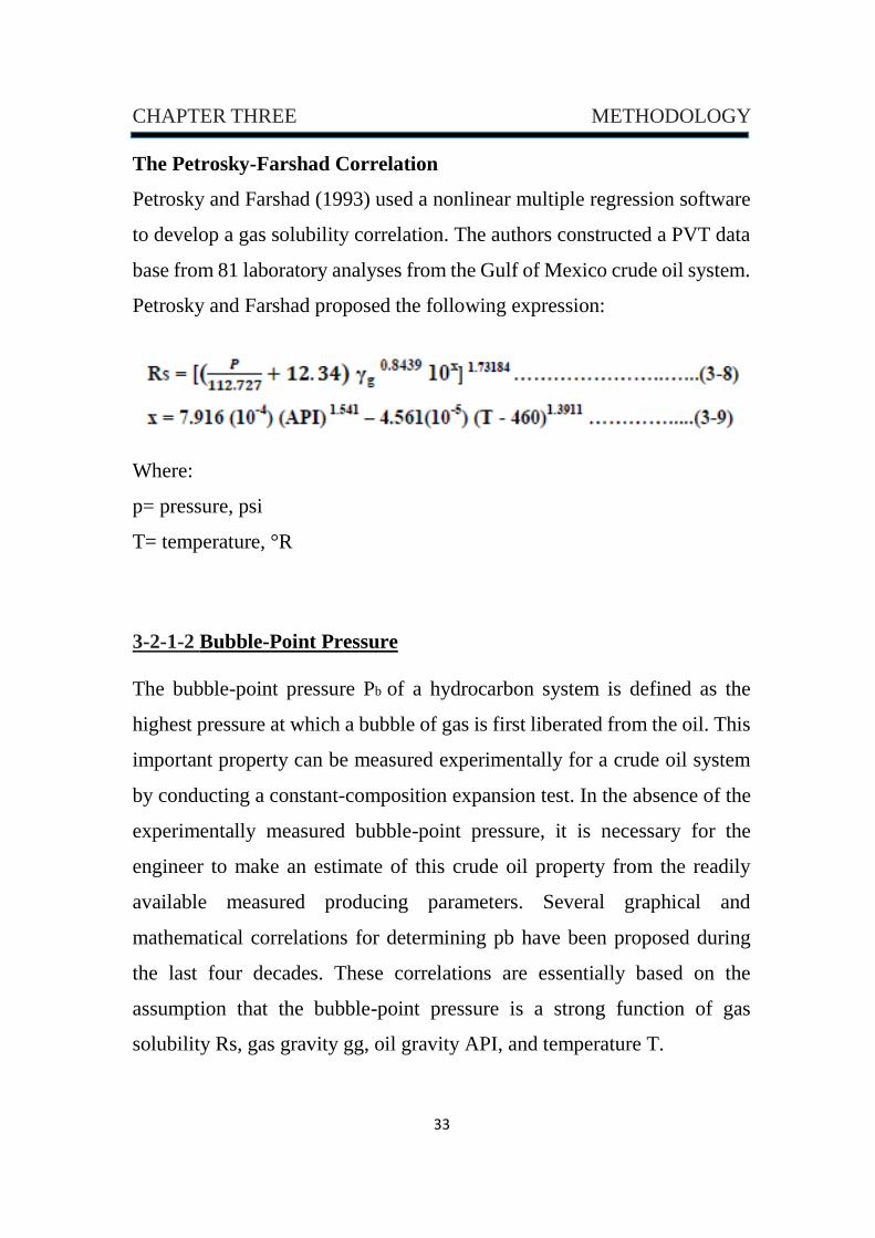
The Petrosky-Farshad Correlation
Petrosky and Farshad (1993) used a nonlinear multiple regression software
to develop a gas solubility correlation. The authors constructed a PVT data
base from 81 laboratory analyses from the Gulf of Mexico crude oil system.
Petrosky and Farshad proposed the following expression:
Where:
p= pressure, psi
T= temperature, °R
3-2-1-2 Bubble-Point Pressure
The bubble-point pressure Pb of a hydrocarbon system is defined as the
highest pressure at which a bubble of gas is first liberated from the oil. This
important property can be measured experimentally for a crude oil system
by conducting a constant-composition expansion test. In the absence of the
experimentally measured bubble-point pressure, it is necessary for the
engineer to make an estimate of this crude oil property from the readily
available measured producing parameters. Several graphical and
mathematical correlations for determining pb have been proposed during
the last four decades. These correlations are essentially based on the
assumption that the bubble-point pressure is a strong function of gas
solubility Rs, gas gravity gg, oil gravity API, and temperature T.
34
CHAPTER THREE METHODOLOGY
Several ways of combining the above parameters in a graphical form or a
mathematical expression are proposed by numerous authors, including:
- Standing
- Vasquez and Beggs
- Glaso
- Marhoun
- Petrosky and Farshad
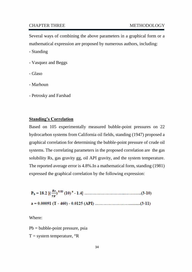
Standing’s Correlation
Based on 105 experimentally measured bubble-point pressures on 22
hydrocarbon systems from California oil fields, standing (1947) proposed a
graphical correlation for determining the bubble-point pressure of crude oil
systems. The correlating parameters in the proposed correlation are the gas
solubility Rs, gas gravity gg, oil API gravity, and the system temperature.
The reported average error is 4.8%.In a mathematical form, standing (1981)
expressed the graphical correlation by the following expression:
Where:
Pb = bubble-point pressure, psia
T = system temperature, °R
35
CHAPTER THREE METHODOLOGY
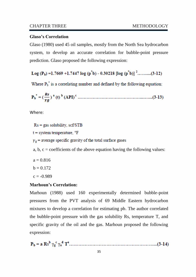
Glaso’s Correlation
Glaso (1980) used 45 oil samples, mostly from the North Sea hydrocarbon
system, to develop an accurate correlation for bubble-point pressure
prediction. Glaso proposed the following expression:
Where:
a, b, c = coefficients of the above equation having the following values:
a = 0.816
b = 0.172
c = -0.989
Marhoun’s Correlation:
Marhoun (1988) used 160 experimentally determined bubble-point
pressures from the PVT analysis of 69 Middle Eastern hydrocarbon
mixtures to develop a correlation for estimating pb. The author correlated
the bubble-point pressure with the gas solubility Rs, temperature T, and
specific gravity of the oil and the gas. Marhoun proposed the following
expression:
36
CHAPTER THREE METHODOLOGY
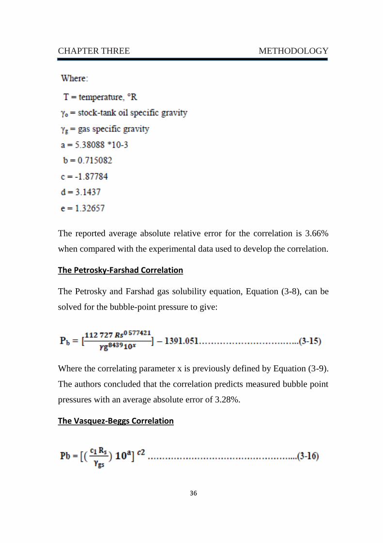
The reported average absolute relative error for the correlation is 3.66%
when compared with the experimental data used to develop the correlation.
The Petrosky-Farshad Correlation
The Petrosky and Farshad gas solubility equation, Equation (3-8), can be
solved for the bubble-point pressure to give:
Where the correlating parameter x is previously defined by Equation (3-9).
The authors concluded that the correlation predicts measured bubble point
pressures with an average absolute error of 3.28%.
The Vasquez-Beggs Correlation
37
CHAPTER THREE METHODOLOGY
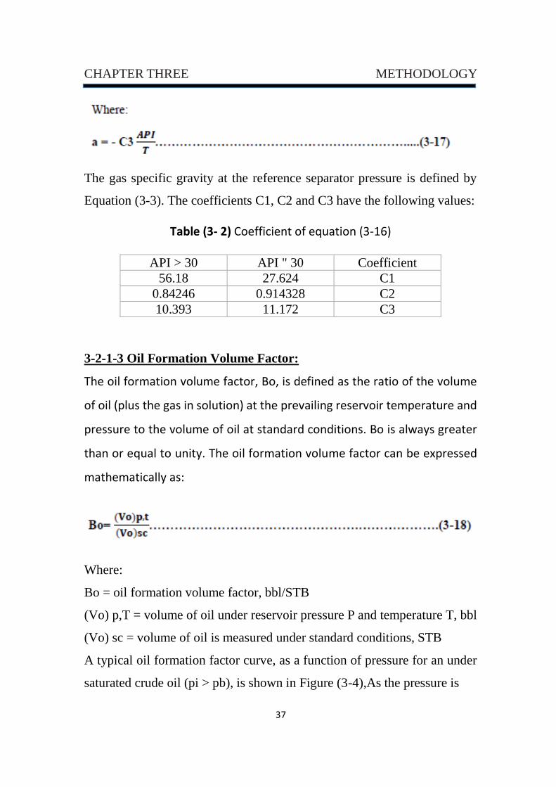
The gas specific gravity at the reference separator pressure is defined by
Equation (3-3). The coefficients C1, C2 and C3 have the following values:
Table (3- 2) Coefficient of equation (3-16)
Coefficient API " 30 API > 30
C1 27.624 56.18
C2 0.914328 0.84246
C3 11.172 10.393
3-2-1-3 Oil Formation Volume Factor:
The oil formation volume factor, Bo, is defined as the ratio of the volume
of oil (plus the gas in solution) at the prevailing reservoir temperature and
pressure to the volume of oil at standard conditions. Bo is always greater
than or equal to unity. The oil formation volume factor can be expressed
mathematically as:
Where:
Bo = oil formation volume factor, bbl/STB
(Vo) p,T = volume of oil under reservoir pressure P and temperature T, bbl
(Vo) sc = volume of oil is measured under standard conditions, STB
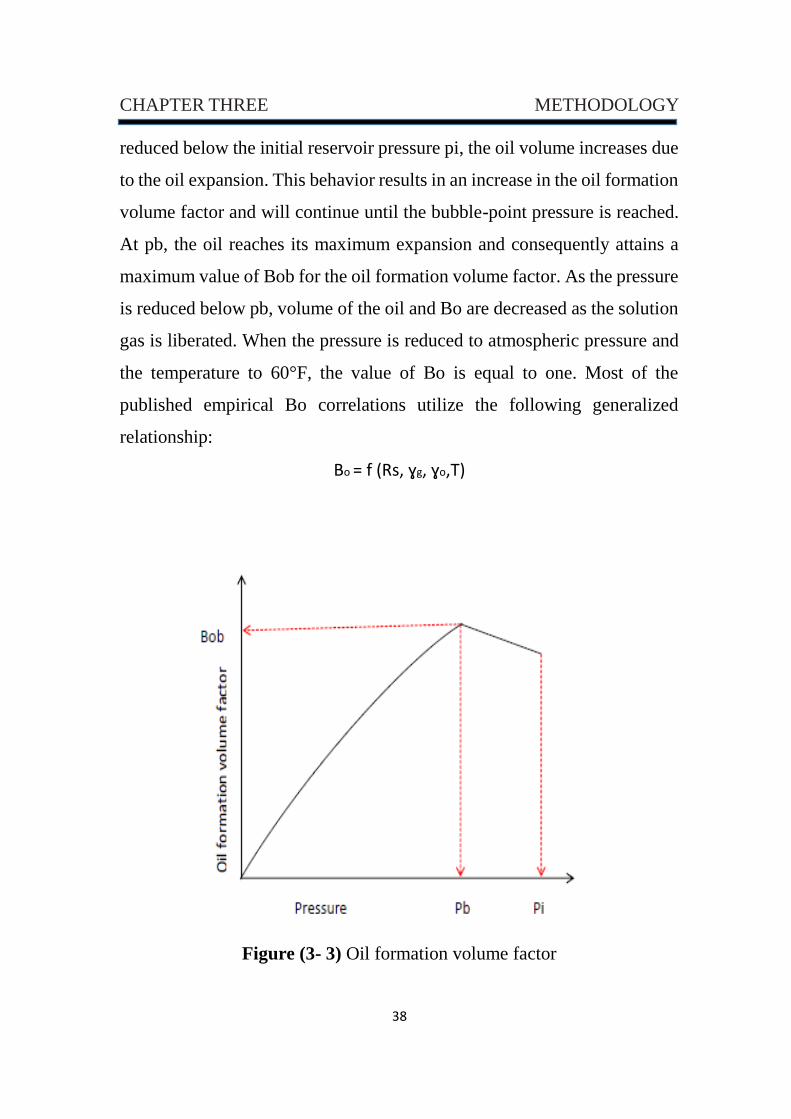
A typical oil formation factor curve, as a function of pressure for an under
saturated crude oil (pi > pb), is shown in Figure (3-4),As the pressure is
38
CHAPTER THREE METHODOLOGY
reduced below the initial reservoir pressure pi, the oil volume increases due
to the oil expansion. This behavior results in an increase in the oil formation
volume factor and will continue until the bubble-point pressure is reached.
At pb, the oil reaches its maximum expansion and consequently attains a
maximum value of Bob for the oil formation volume factor. As the pressure
is reduced below pb, volume of the oil and Bo are decreased as the solution
gas is liberated. When the pressure is reduced to atmospheric pressure and
the temperature to 60°F, the value of Bo is equal to one. Most of the
published empirical Bo correlations utilize the following generalized
relationship:
Bo = f (Rs, ɣg, ɣo,T)
Figure (3- 3) Oil formation volume factor
39
CHAPTER THREE METHODOLOGY
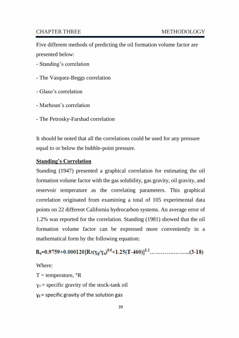
Five different methods of predicting the oil formation volume factor are
presented below:
- Standing’s correlation
- The Vasquez-Beggs correlation
- Glaso’s correlation
- Marhoun’s correlation
- The Petrosky-Farshad correlation
It should be noted that all the correlations could be used for any pressure
equal to or below the bubble-point pressure.
Standing’s Correlation
Standing (1947) presented a graphical correlation for estimating the oil
formation volume factor with the gas solubility, gas gravity, oil gravity, and
reservoir temperature as the correlating parameters. This graphical
correlation originated from examining a total of 105 experimental data
points on 22 different California hydrocarbon systems. An average error of
1.2% was reported for the correlation. Standing (1981) showed that the oil
formation volume factor can be expressed more conveniently in a
mathematical form by the following equation:
Where:
T = temperature, °R
ɣo = specific gravity of the stock-tank oil
ɣg = specific gravity of the solution gas
40
CHAPTER THREE METHODOLOGY
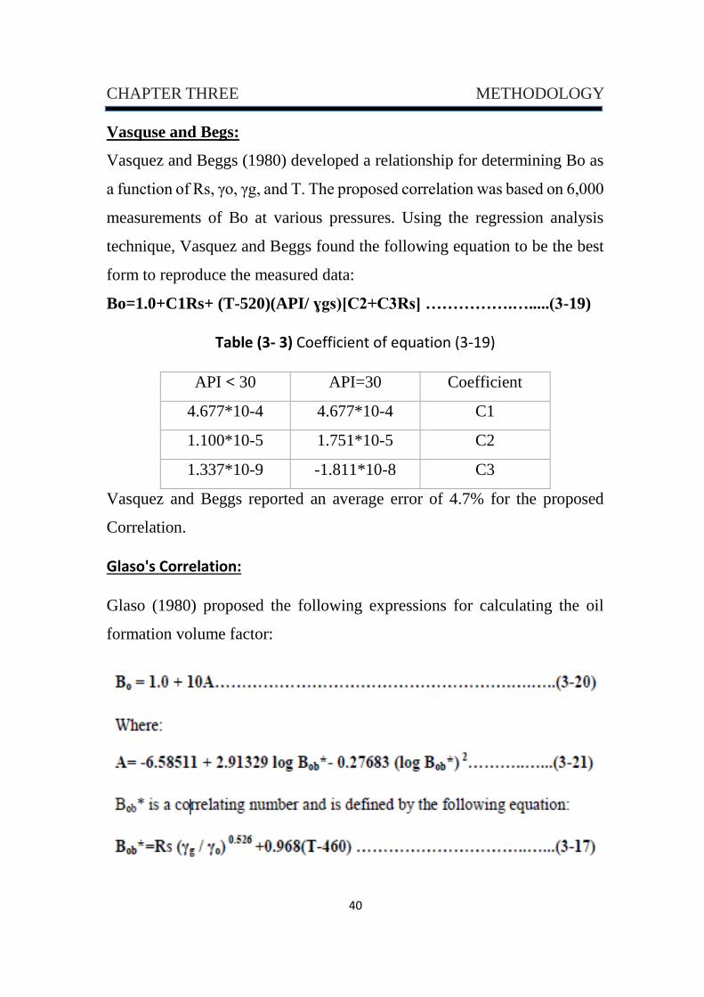
Vasquse and Begs:
Vasquez and Beggs (1980) developed a relationship for determining Bo as
a function of Rs, γo, γg, and T. The proposed correlation was based on 6,000
measurements of Bo at various pressures. Using the regression analysis
technique, Vasquez and Beggs found the following equation to be the best
form to reproduce the measured data:
Bo=1.0+C1Rs+ (T-520)(API/ ɣgs)[C2+C3Rs] …………….….....(3-19)
Table (3- 3) Coefficient of equation (3-19)
Coefficient API=30 API < 30
C1 4.677*10-4 4.677*10-4
C2 1.751*10-5 1.100*10-5
C3 -1.811*10-8 1.337*10-9
Vasquez and Beggs reported an average error of 4.7% for the proposed
Correlation.
Glaso's Correlation:
Glaso (1980) proposed the following expressions for calculating the oil
formation volume factor:
41
CHAPTER THREE METHODOLOGY
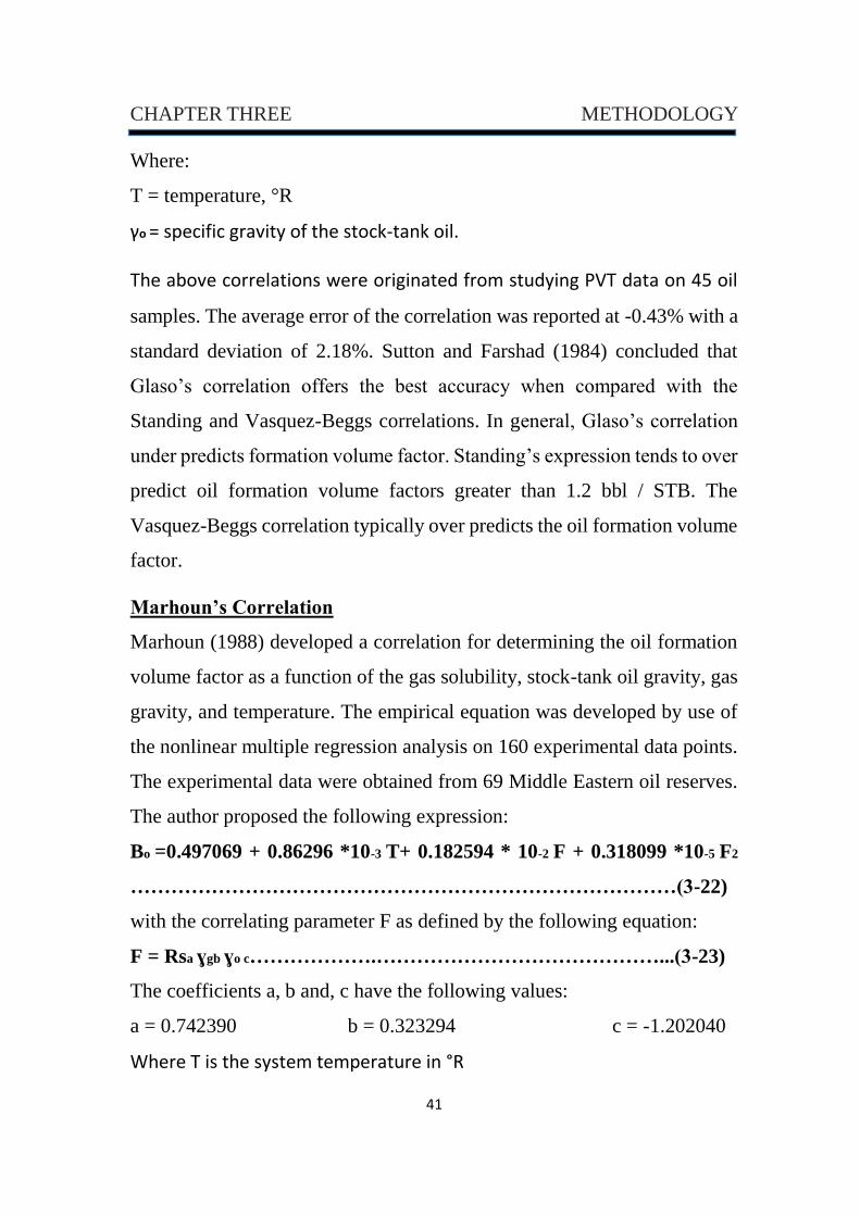
Where:
T = temperature, °R
γo = specific gravity of the stock-tank oil.
The above correlations were originated from studying PVT data on 45 oil
samples. The average error of the correlation was reported at -0.43% with a
standard deviation of 2.18%. Sutton and Farshad (1984) concluded that
Glaso’s correlation offers the best accuracy when compared with the
Standing and Vasquez-Beggs correlations. In general, Glaso’s correlation
under predicts formation volume factor. Standing’s expression tends to over
predict oil formation volume factors greater than 1.2 bbl / STB. The
Vasquez-Beggs correlation typically over predicts the oil formation volume
factor.
Marhoun’s Correlation
Marhoun (1988) developed a correlation for determining the oil formation
volume factor as a function of the gas solubility, stock-tank oil gravity, gas
gravity, and temperature. The empirical equation was developed by use of
the nonlinear multiple regression analysis on 160 experimental data points.
The experimental data were obtained from 69 Middle Eastern oil reserves.
The author proposed the following expression:
Bo =0.497069 + 0.86296 *10-3 T+ 0.182594 * 10-2 F + 0.318099 *10-5 F2
………………………………………………………………………(3-22)
with the correlating parameter F as defined by the following equation:
F = Rsa ɣgb ɣo c……………….……………………………………...(3-23)
The coefficients a, b and, c have the following values:
a = 0.742390 b = 0.323294 c = -1.202040
Where T is the system temperature in °R
42
CHAPTER THREE METHODOLOGY
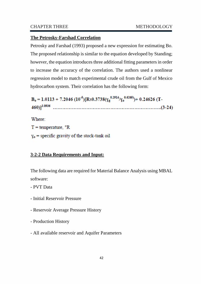
The Petrosky-Farshad Correlation
Petrosky and Farshad (1993) proposed a new expression for estimating Bo.
The proposed relationship is similar to the equation developed by Standing;
however, the equation introduces three additional fitting parameters in order
to increase the accuracy of the correlation. The authors used a nonlinear
regression model to match experimental crude oil from the Gulf of Mexico
hydrocarbon system. Their correlation has the following form:
3-2-2 Data Requirements and Input:
The following data are required for Material Balance Analysis using MBAL
software:
- PVT Data
- Initial Reservoir Pressure
- Reservoir Average Pressure History
- Production History
- All available reservoir and Aquifer Parameters
43
CHAPTER THREE METHODOLOGY
3-2-3 Describing PVT:
To appropriately estimate the reservoir pressure and saturation changes as
fluid is produced throughout the reservoir requires a precise description of
the reservoir fluid properties. To accurately describe these properties, the
ideal process is to sample the reservoir fluid and perform a laboratory
studies on the fluid samples. This is not always possible to continuously
take fluid sample for analysis as the reservoir pressure declines; hence,
engineers have resorted to correlations to generate the fluid properties.
MBAL program uses traditional black oil correlations, such as Petrosky and
Fashad (1993), Standing (1994) and Glaso (1980) etc. The PVT data in this
research obtained from L.P Dake (Chapter 9. Example 9.2), this study
depends on Glaso's correlation.
3-2-4 History Matching:
History matching involves a trial and error approach to provide a best fit
comparison between the observed data and the calculated data on a zero
dimensional level. It comprises the functions of the graphical method, the
analytical method, simulation tests and pseudo-relative permeability
matching techniques. History matching is used to determine and identify
sources of reservoir energy and their magnitude, the value of OOIP, Gi,
aquifer type and strength etc. History matching in MBE is the most effective
way to determine the aquifer model that best fits the observed data.
3-2-5 Water influx
Nearly all hydrocarbon reservoirs are surrounded by water-bearing rocks
called aquifers. These aquifers may be substantially larger than the oil or
gas reservoirs they adjoin as to appear infinite in size, or they may be so
small in size as to be negligible in their effect on reservoir performance. As
44
CHAPTER THREE METHODOLOGY
reservoir fluids are produced and reservoir pressure declines, a pressure
differential develops from the surrounding aquifer into the reservoir.
Following the basic law of fluid flow in porous media, the aquifer reacts by
encroaching across the original hydrocarbon-water contact. In some cases,
water encroachment occurs due to hydrodynamic conditions and recharge
of the formation by surface waters at an outcrop. In many cases, the pore
volume of the aquifer is not significantly larger than the pore volume of the
reservoir itself. Thus, the expansion of the water in the aquifer is negligible
relative to the overall energy system, and the reservoir behaves
volumetrically. In this case, the effects of water influx can be ignored. In
other cases, the aquifer permeability may be sufficiently low such that a
very large pressure differential is required before an appreciable amount of
water can encroach into the reservoir. In this instance, the effects of water
influx can be ignored as well. Several models have been developed for
estimating water influx that is based on assumptions that describe the
characteristics of the aquifer. Due to the inherent uncertainties in the aquifer
characteristics, all of the proposed models require historical reservoir
performance data to evaluate constants representing aquifer property
parameters since these are rarely known from exploration-development
drilling with sufficient accuracy for direct application. The material balance
equation can be used to determine historical water influx provided original
oil-in-place is known from pore volume estimates. This permits evaluation
of the constants in the influx equations so that future water influx rate can
be forecasted. The mathematical water influx models are:
- Pot aquifer
- Schilthuis’steady-state
- Hurst’s modified steady-state
45
CHAPTER THREE METHODOLOGY
- The Van Everdingen-Hurst unsteady-state
- The Carter-Tracy unsteady-state
- Fetkovich’s method
3-2-6 Graphical method
The first step taken was to plot (F /We) / Et versus F (i.e. the withdrawal)
known as Campbell’s plot with no aquifer defined initially. If there is no
other source of reservoir energy other than the total fluid expansion Et, then
this Campbell’s plot will be a horizontal straight line with a Y axis intercept
equal to the original oil in place (OOIP). Any “turn-up” in the plot (i.e.
deviation from the theoretical horizontal straight line) indicates another
source of energy present (due to a source (injector) or an aquifer influx).
3-2-7 Analytical method
The analytical method allows for regression on all reservoir model
parameters. Regression is used to adjust the reservoir model to minimize
the difference between the observed/measured and the model production. It
is used to assess the effects of varying parameters such as formation
compressibility that cannot easily be assessed using graphical methods.
The quality of the regression match is expressed as the standard deviation
between model and measured values. The analytical plot was regressed to
compute the oil in place, the encroachment angle, and the aquifer
permeability, inner and outer radius
3-2-8 Energy Plot
The plot describes the prevalent energy system present in the reservoir;
water influx, pore volume compressibility, fluid expansion, ingestions etc.
It describes the fractional contributions of these energy systems present in
the reservoir and the most prominent at various date.
46
CHAPTER THREE METHODOLOGY
3-3 Decline curve analysis
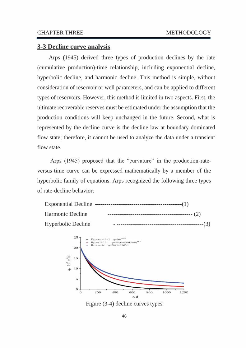
Arps (1945) derived three types of production declines by the rate
(cumulative production)-time relationship, including exponential decline,
hyperbolic decline, and harmonic decline. This method is simple, without
consideration of reservoir or well parameters, and can be applied to different
types of reservoirs. However, this method is limited in two aspects. First, the
ultimate recoverable reserves must be estimated under the assumption that the
production conditions will keep unchanged in the future. Second, what is
represented by the decline curve is the decline law at boundary dominated
flow state; therefore, it cannot be used to analyze the data under a transient
flow state.
Arps (1945) proposed that the “curvature” in the production-rate-
versus-time curve can be expressed mathematically by a member of the
hyperbolic family of equations. Arps recognized the following three types
of rate-decline behavior:
Exponential Decline ---------------------------------------------(1)
Harmonic Decline -------------------------------------------- (2)
Hyperbolic Decline - ---------------------------------------------(3)
Figure (3-4) decline curves types
47
CHAPTER THREE METHODOLOGY
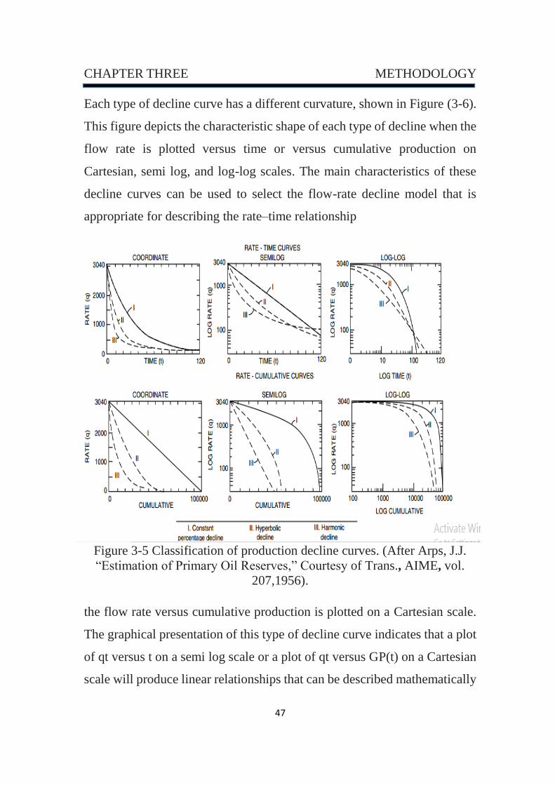
Each type of decline curve has a different curvature, shown in Figure (3-6).
This figure depicts the characteristic shape of each type of decline when the
flow rate is plotted versus time or versus cumulative production on
Cartesian, semi log, and log-log scales. The main characteristics of these
decline curves can be used to select the flow-rate decline model that is
appropriate for describing the rate–time relationship
Figure 3-5 Classification of production decline curves. (After Arps, J.J.
“Estimation of Primary Oil Reserves,” Courtesy of Trans., AIME, vol.
207,1956).
the flow rate versus cumulative production is plotted on a Cartesian scale.
The graphical presentation of this type of decline curve indicates that a plot
of qt versus t on a semi log scale or a plot of qt versus GP(t) on a Cartesian
scale will produce linear relationships that can be described mathematically
48
CHAPTER THREE METHODOLOGY
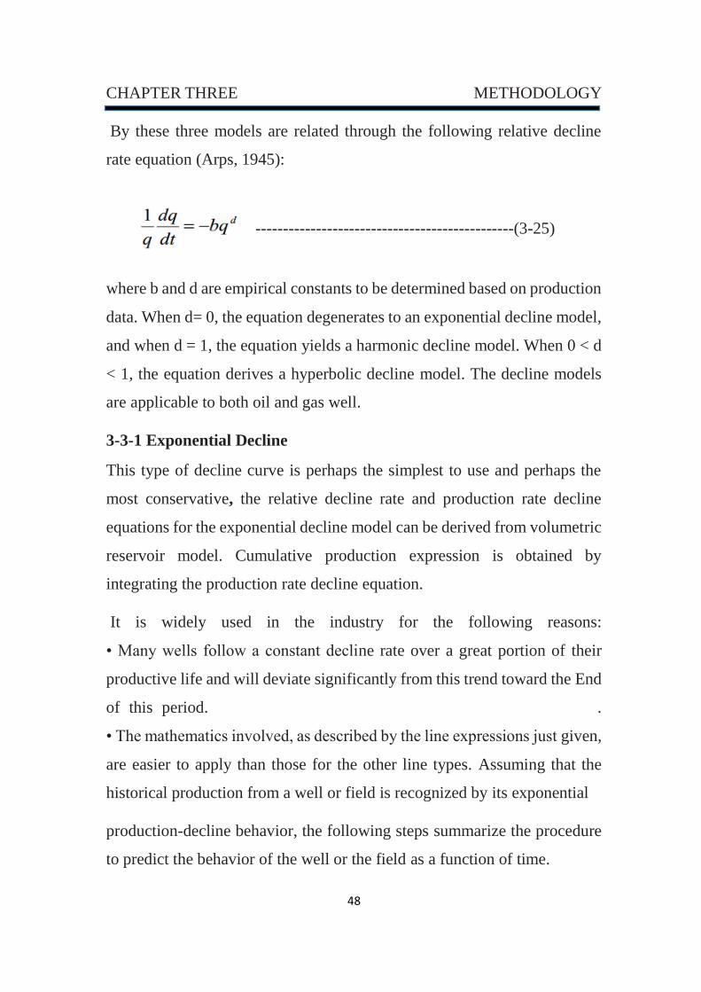
By these three models are related through the following relative decline
rate equation (Arps, 1945):
-----------------------------------------------(3-25)
where b and d are empirical constants to be determined based on production
data. When d= 0, the equation degenerates to an exponential decline model,
and when d = 1, the equation yields a harmonic decline model. When 0 < d
< 1, the equation derives a hyperbolic decline model. The decline models
are applicable to both oil and gas well.
3-3-1 Exponential Decline
This type of decline curve is perhaps the simplest to use and perhaps the
most conservative, the relative decline rate and production rate decline
equations for the exponential decline model can be derived from volumetric
reservoir model. Cumulative production expression is obtained by
integrating the production rate decline equation.
It is widely used in the industry for the following reasons:
• Many wells follow a constant decline rate over a great portion of their
productive life and will deviate significantly from this trend toward the End
of this period. .
• The mathematics involved, as described by the line expressions just given,
are easier to apply than those for the other line types. Assuming that the
historical production from a well or field is recognized by its exponential
production-decline behavior, the following steps summarize the procedure
to predict the behavior of the well or the field as a function of time.
49
CHAPTER THREE METHODOLOGY
production-decline behavior, the following steps summarize the procedure
to predict the behavior of the well or the field as a function of time.
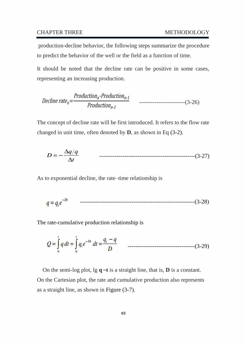
It should be noted that the decline rate can be positive in some cases,
representing an increasing production.
------------------------(3-26)
The concept of decline rate will be first introduced. It refers to the flow rate
changed in unit time, often denoted by D, as shown in Eq (3-2).
--------------------------------------------------(3-27)
As to exponential decline, the rate–time relationship is
------------------------------------------------------------(3-28)
The rate-cumulative production relationship is
-----------------------------------(3-29)
On the semi-log plot, lg q∼t is a straight line, that is, D is a constant.
On the Cartesian plot, the rate and cumulative production also represents
as a straight line, as shown in Figure (3-7).
50
CHAPTER THREE METHODOLOGY
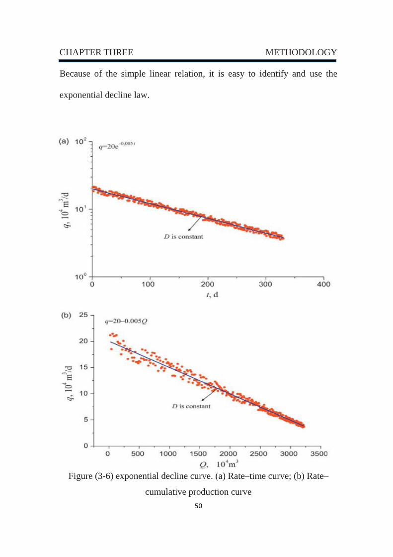
Because of the simple linear relation, it is easy to identify and use the
exponential decline law.
Figure (3-6) exponential decline curve. (a) Rate–time curve; (b) Rate–
cumulative production curve
51
CHAPTER THREE METHODOLOGY
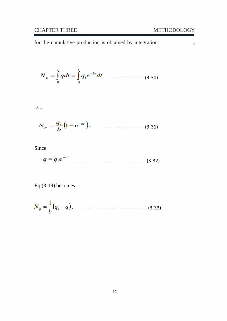
for the cumulative production is obtained by integration: ,
--------------------(3-30)
i.e.,
---------------------------(3-31)
Since
--------------------------------------------(3-32)
Eq (3-19) becomes
----------------------------------------(3-33)
52
CHAPTER THREE METHODOLOGY
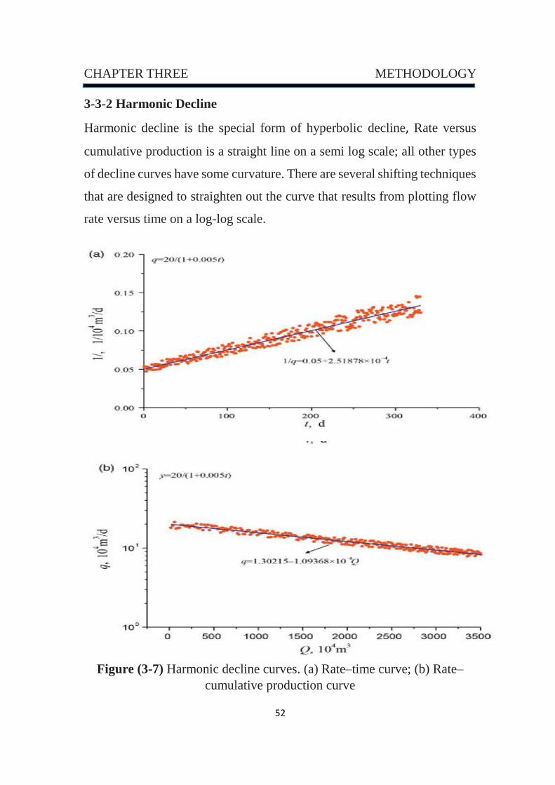
3-3-2 Harmonic Decline
Harmonic decline is the special form of hyperbolic decline, Rate versus
cumulative production is a straight line on a semi log scale; all other types
of decline curves have some curvature. There are several shifting techniques
that are designed to straighten out the curve that results from plotting flow
rate versus time on a log-log scale.
Figure (3-7) Harmonic decline curves. (a) Rate–time curve; (b) Rate–
cumulative production curve
53
CHAPTER THREE METHODOLOGY
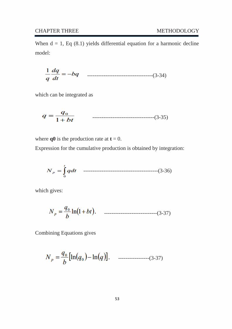
When d = 1, Eq (8.1) yields differential equation for a harmonic decline
model:
------------------------------------(3-34)
which can be integrated as
----------------------------------(3-35)
where q0 is the production rate at t = 0.
Expression for the cumulative production is obtained by integration:
-----------------------------------------(3-36)
which gives:
-----------------------------(3-37)
Combining Equations gives
-----------------(3-37)
54
CHAPTER THREE METHODOLOGY
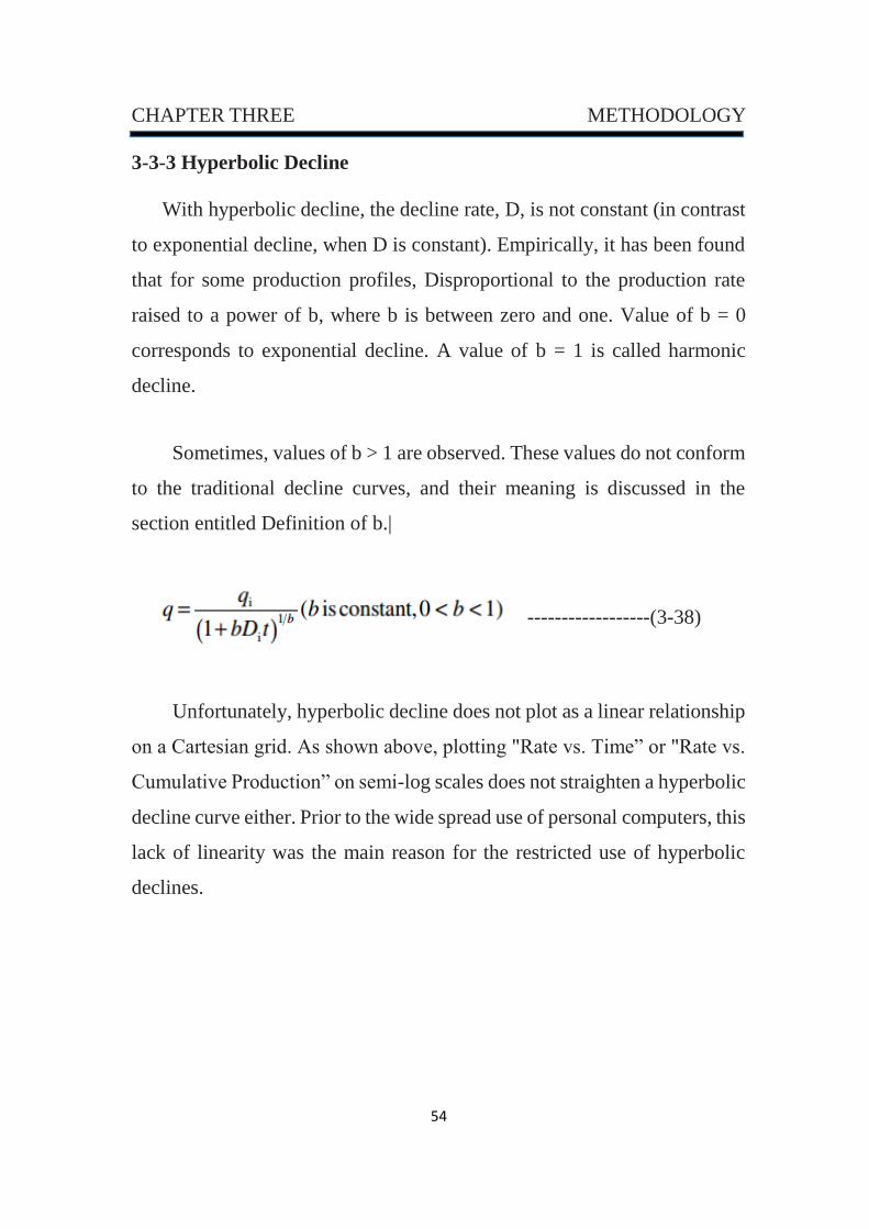
3-3-3 Hyperbolic Decline
With hyperbolic decline, the decline rate, D, is not constant (in contrast
to exponential decline, when D is constant). Empirically, it has been found
that for some production profiles, Disproportional to the production rate
raised to a power of b, where b is between zero and one. Value of b = 0
corresponds to exponential decline. A value of b = 1 is called harmonic
decline.
Sometimes, values of b > 1 are observed. These values do not conform
to the traditional decline curves, and their meaning is discussed in the
section entitled Definition of b.|
------------------(3-38)
Unfortunately, hyperbolic decline does not plot as a linear relationship
on a Cartesian grid. As shown above, plotting "Rate vs. Time” or "Rate vs.
Cumulative Production” on semi-log scales does not straighten a hyperbolic
decline curve either. Prior to the wide spread use of personal computers, this
lack of linearity was the main reason for the restricted use of hyperbolic
declines.
55
CHAPTER THREE METHODOLOGY
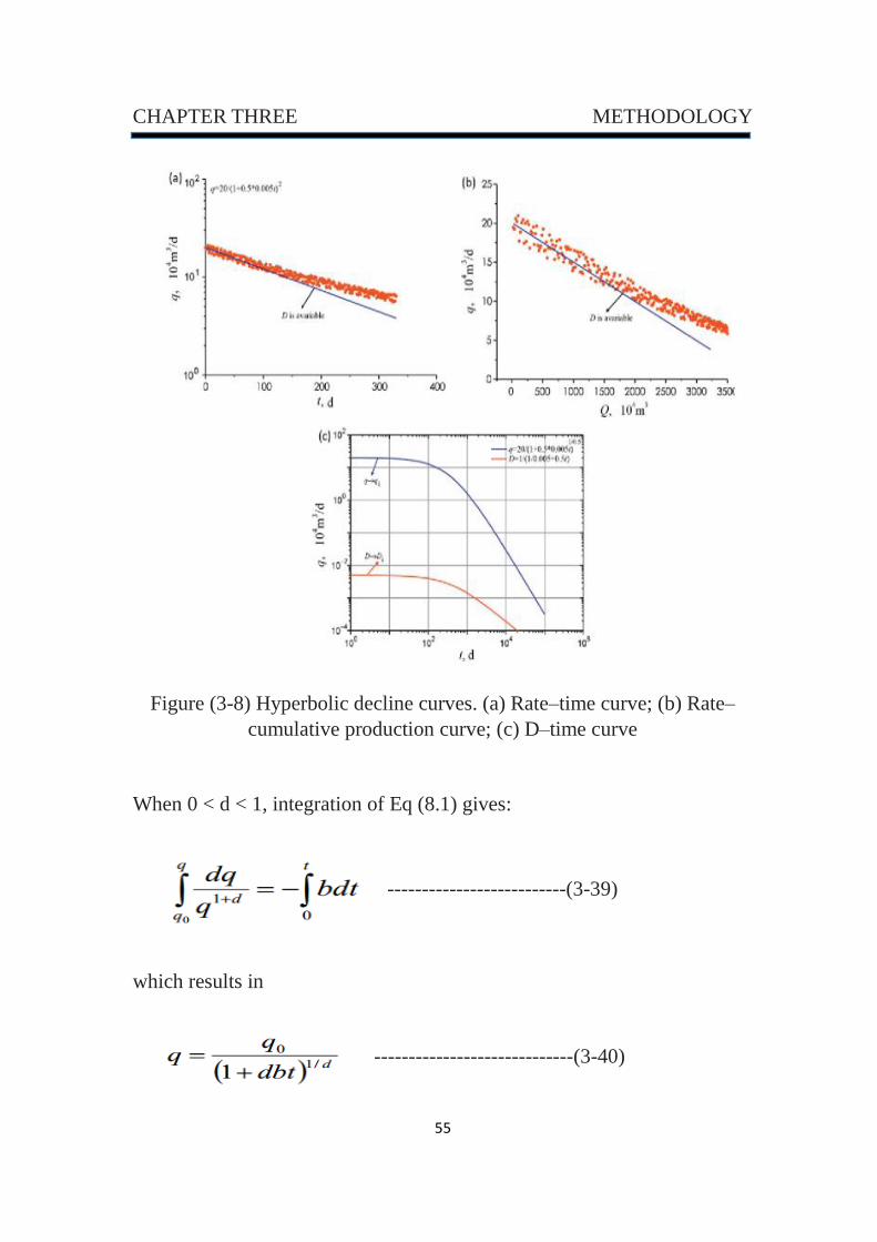
Figure (3-8) Hyperbolic decline curves. (a) Rate–time curve; (b) Rate–
cumulative production curve; (c) D–time curve
When 0 < d < 1, integration of Eq (8.1) gives:
--------------------------(3-39)
which results in
-----------------------------(3-40)
56
CHAPTER THREE METHODOLOGY
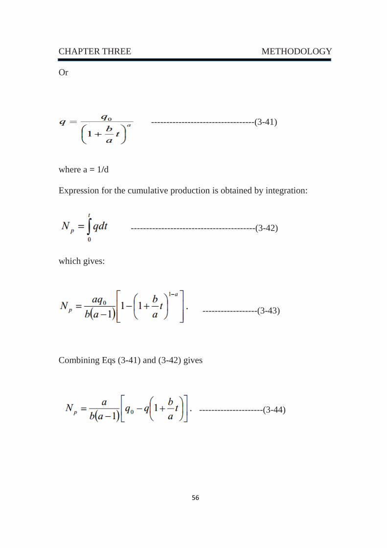
Or
----------------------------------(3-41)
where a = 1/d
Expression for the cumulative production is obtained by integration:
-----------------------------------------(3-42)
which gives:
------------------(3-43)
Combining Eqs (3-41) and (3-42) gives
---------------------(3-44)
57
CHAPTER THREE METHODOLOGY
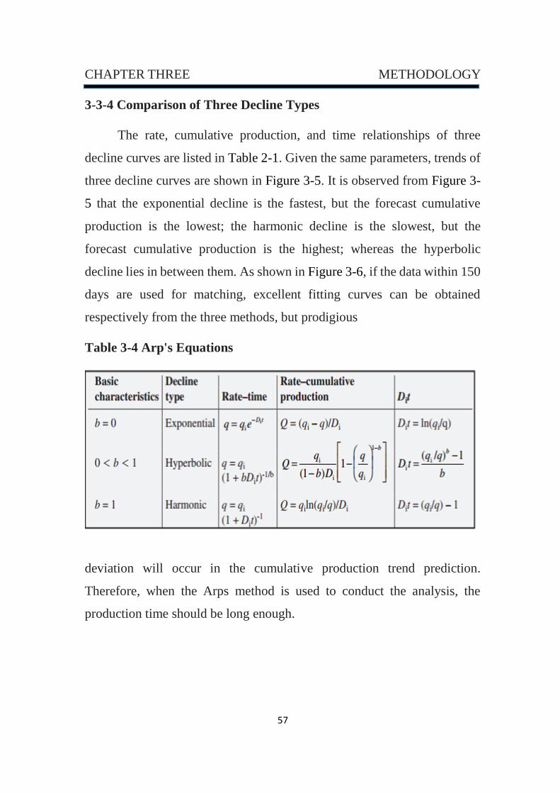
3-3-4 Comparison of Three Decline Types
The rate, cumulative production, and time relationships of three
decline curves are listed in Table 2-1. Given the same parameters, trends of
three decline curves are shown in Figure 3-5. It is observed from Figure 3-
5 that the exponential decline is the fastest, but the forecast cumulative
production is the lowest; the harmonic decline is the slowest, but the
forecast cumulative production is the highest; whereas the hyperbolic
decline lies in between them. As shown in Figure 3-6, if the data within 150
days are used for matching, excellent fitting curves can be obtained
respectively from the three methods, but prodigious
Table 3-4 Arp's Equations
deviation will occur in the cumulative production trend prediction.
Therefore, when the Arps method is used to conduct the analysis, the
production time should be long enough.
58
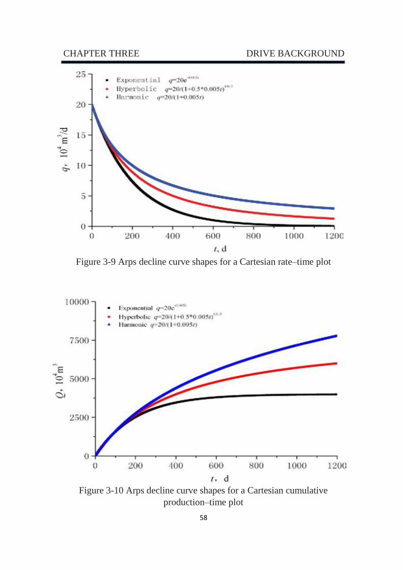
CHAPTER THREE DRIVE BACKGROUND
Figure 3-9 Arps decline curve shapes for a Cartesian rate–time plot
Figure 3-10 Arps decline curve shapes for a Cartesian cumulative
production–time plot

59
CHAPTER FOUR CALCULATION AND RESULT
Chapter Four
CALCULATIONS AND RESULTS
The present work provides two methods for reservoir performance
prediction. Material balance and decline curve analysis methods are used to
calculating initial oil in place, estimate the recoverable hydrocarbon and the
future performance of the reservoir or well. The methods are applied for data
from L.P Dake (example 9.2). Also we used decline curve analysis method to
determine the future performance and remaining recoverable oil for data
from AL-halfya, zubair, nahr umr and bzrgan fields.
4-1 Data required for Material balance and Decline curve methods
The material balance and decline curve analysis methods applied for well
production data is a good technique to forecast future performance of a well or
the fields under study. The input data required to use these methods are as
shown below:
- PVT Data
- Initial Reservoir Pressure
- Reservoir Average Pressure History
- Production History
- All Available Reservoir and Aquifer Parameters
60
CHAPTER FOUR CALCULATIONS AND RESULTS
4-2 RESULTS AND DISCUSSION
4-2-1Matereal balance method
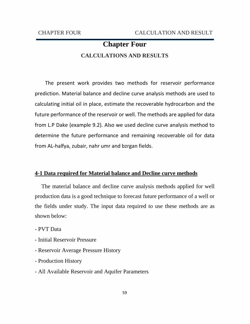
4-2-1-1 PVT Data:
The data used in this study were obtained from Dake's book. (4-1) illustrates
that.
Figure (4- 1) oil black matching
The correlation that gives least standard deviation is the correlation that has
best match. We can see that Glaso correlation is the least standard deviation
so the program will base on this correlation in the calculation.
61
CHAPTER FOUR CALCULATIONS AND RESULTS
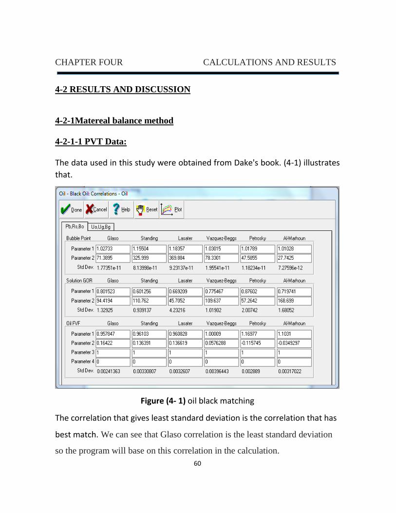
the type of reservoir is saturated reservoir and this shown clearly in the plot
of the Bo versus pressure because Pi = Pb , Figure (4-2)
Figure (4- 2) Plot of FVF versus Pressure
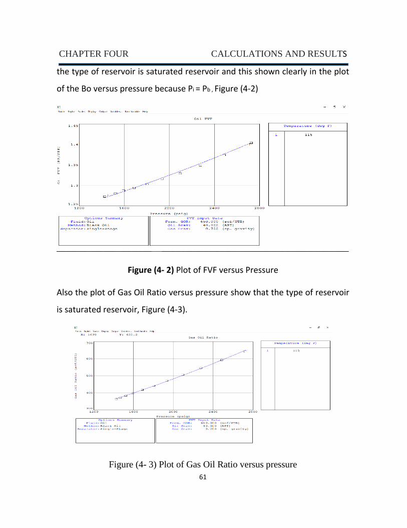
Also the plot of Gas Oil Ratio versus pressure show that the type of reservoir
is saturated reservoir, Figure (4-3).
Figure (4- 3) Plot of Gas Oil Ratio versus pressure
62
CHAPTER FOUR CALCULATIONS AND RESULTS
4-2-1-2 History Matching
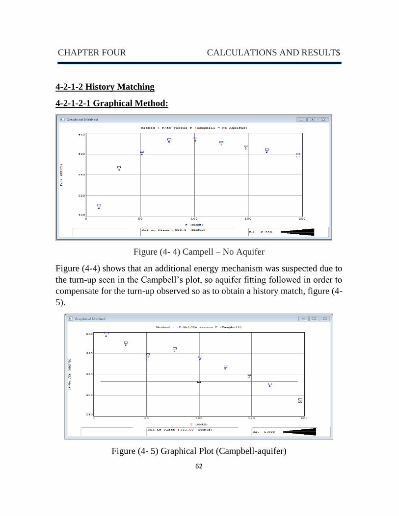
4-2-1-2-1 Graphical Method:
Figure (4- 4) Campell – No Aquifer
Figure (4-4) shows that an additional energy mechanism was suspected due to
the turn-up seen in the Campbell’s plot, so aquifer fitting followed in order to
compensate for the turn-up observed so as to obtain a history match, figure (4-
5).
Figure (4- 5) Graphical Plot (Campbell-aquifer)
63
CHAPTER FOUR CALCULATIONS AND RESULTS
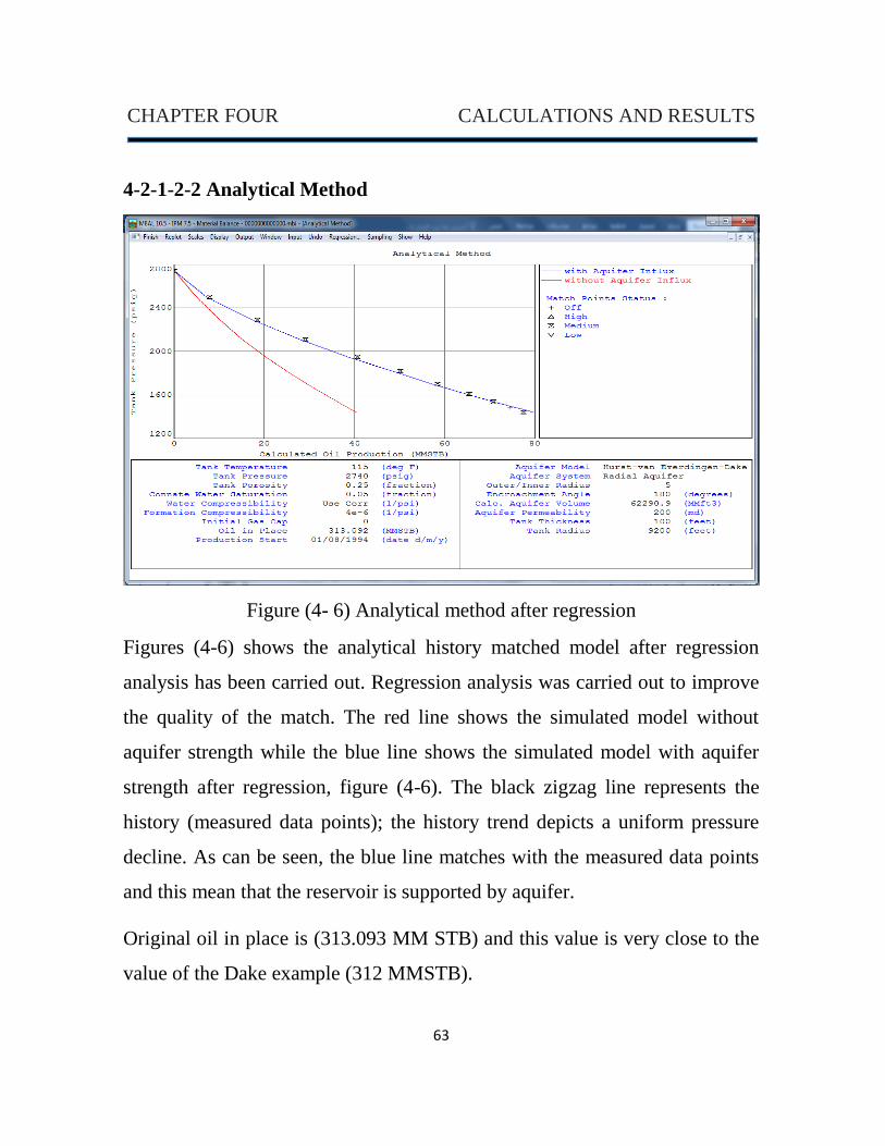
4-2-1-2-2 Analytical Method
Figure (4- 6) Analytical method after regression
Figures (4-6) shows the analytical history matched model after regression
analysis has been carried out. Regression analysis was carried out to improve
the quality of the match. The red line shows the simulated model without
aquifer strength while the blue line shows the simulated model with aquifer
strength after regression, figure (4-6). The black zigzag line represents the
history (measured data points); the history trend depicts a uniform pressure
decline. As can be seen, the blue line matches with the measured data points
and this mean that the reservoir is supported by aquifer.
Original oil in place is (313.093 MM STB) and this value is very close to the
value of the Dake example (312 MMSTB).
64
CHAPTER FOUR CALCULATIONS AND RESULTS
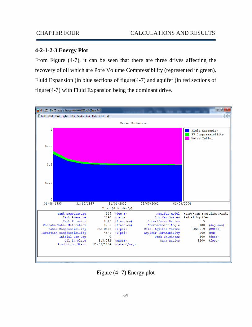
4-2-1-2-3 Energy Plot
From Figure (4-7), it can be seen that there are three drives affecting the
recovery of oil which are Pore Volume Compressibility (represented in green).
Fluid Expansion (in blue sections of figure(4-7) and aquifer (in red sections of
figure(4-7) with Fluid Expansion being the dominant drive.
Figure (4- 7) Energy plot
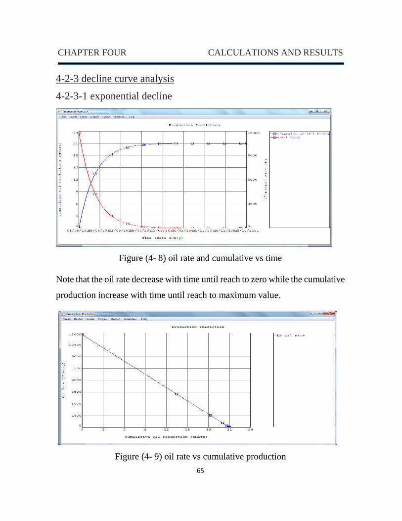
65
CHAPTER FOUR CALCULATIONS AND RESULTS
4-2-3 decline curve analysis
4-2-3-1 exponential decline
Figure (4- 8) oil rate and cumulative vs time
Note that the oil rate decrease with time until reach to zero while the cumulative
production increase with time until reach to maximum value.
Figure (4- 9) oil rate vs cumulative production
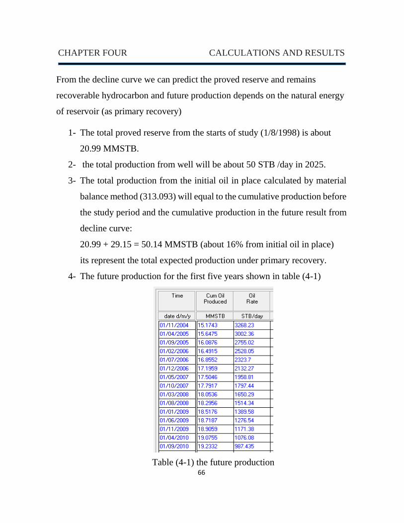
66
CHAPTER FOUR CALCULATIONS AND RESULTS
From the decline curve we can predict the proved reserve and remains
recoverable hydrocarbon and future production depends on the natural energy
of reservoir (as primary recovery)
1- The total proved reserve from the starts of study (1/8/1998) is about
20.99 MMSTB.
2- the total production from well will be about 50 STB /day in 2025.
3- The total production from the initial oil in place calculated by material
balance method (313.093) will equal to the cumulative production before
the study period and the cumulative production in the future result from
decline curve:
20.99 + 29.15 = 50.14 MMSTB (about 16% from initial oil in place)
its represent the total expected production under primary recovery.
4- The future production for the first five years shown in table (4-1)
Table (4-1) the future production
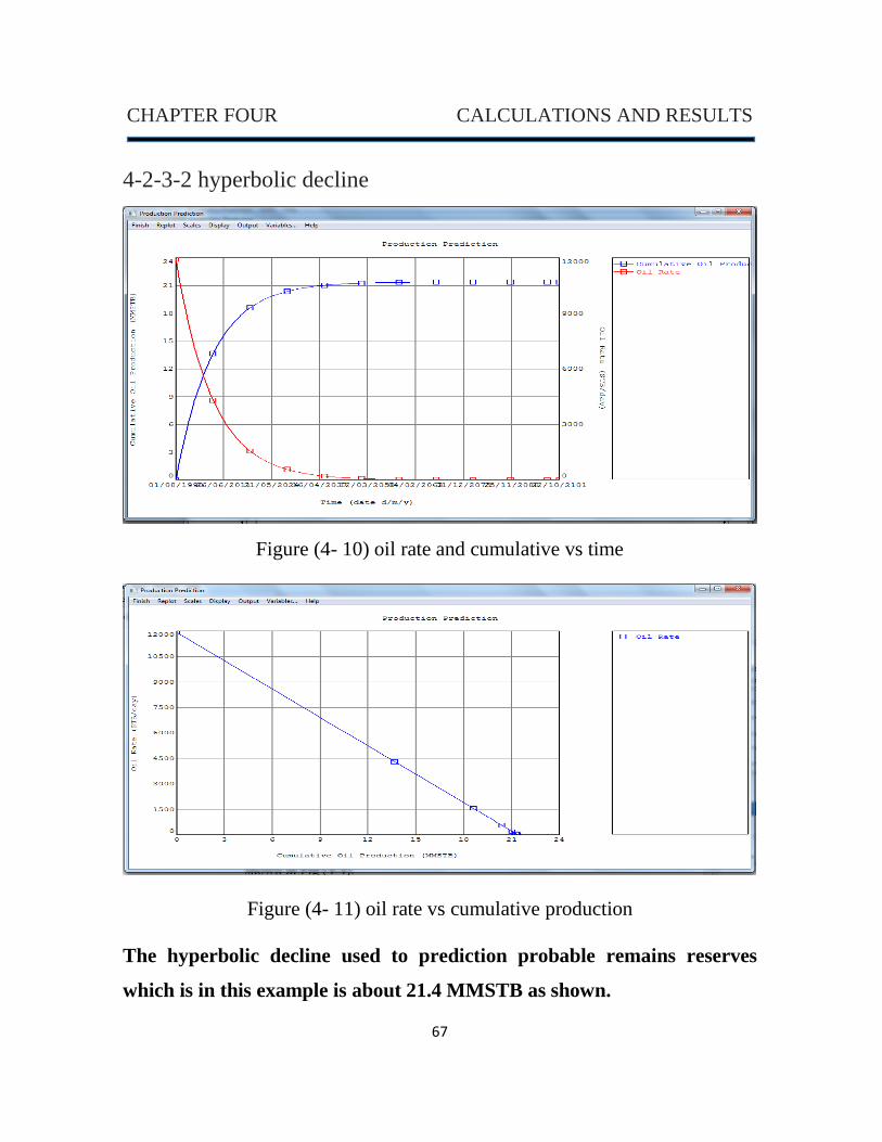
67
CHAPTER FOUR CALCULATIONS AND RESULTS
4-2-3-2 hyperbolic decline
Figure (4- 10) oil rate and cumulative vs time
Figure (4- 11) oil rate vs cumulative production
The hyperbolic decline used to prediction probable remains reserves
which is in this example is about 21.4 MMSTB as shown.
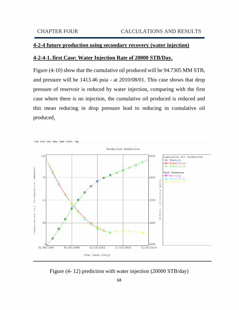
68
CHAPTER FOUR CALCULATIONS AND RESULTS
4-2-4 future production using secondary recovery (water injection)
4-2-4-1. first Case: Water Injection Rate of 20000 STB/Day.
Figure (4-10) show that the cumulative oil produced will be 94.7305 MM STB,
and pressure will be 1413.46 psia - at 2010/08/01. This case shows that drop
pressure of reservoir is reduced by water injection, comparing with the first
case where there is no injection, the cumulative oil produced is reduced and
this mean reducing in drop pressure lead to reducing in cumulative oil
produced.
Figure (4- 12) prediction with water injection (20000 STB/day)
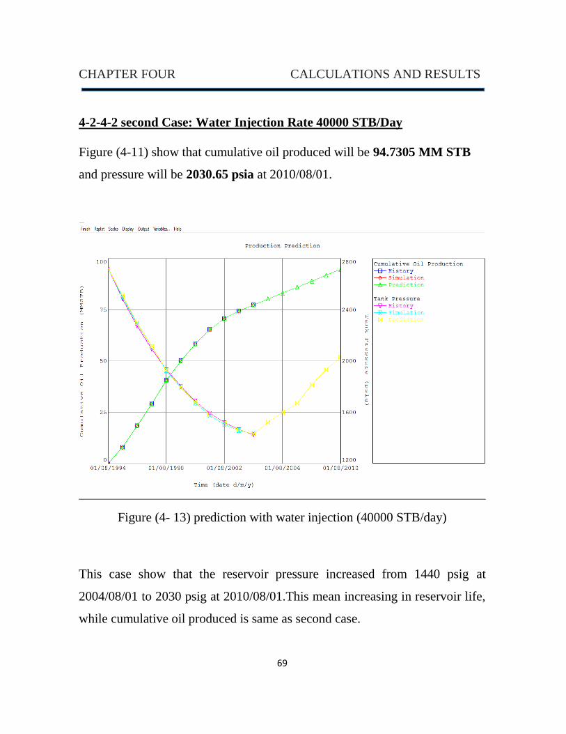
69
CHAPTER FOUR CALCULATIONS AND RESULTS
4-2-4-2 second Case: Water Injection Rate 40000 STB/Day
Figure (4-11) show that cumulative oil produced will be 94.7305 MM STB
and pressure will be 2030.65 psia at 2010/08/01.
Figure (4- 13) prediction with water injection (40000 STB/day)
This case show that the reservoir pressure increased from 1440 psig at
2004/08/01 to 2030 psig at 2010/08/01.This mean increasing in reservoir life,
while cumulative oil produced is same as second case.
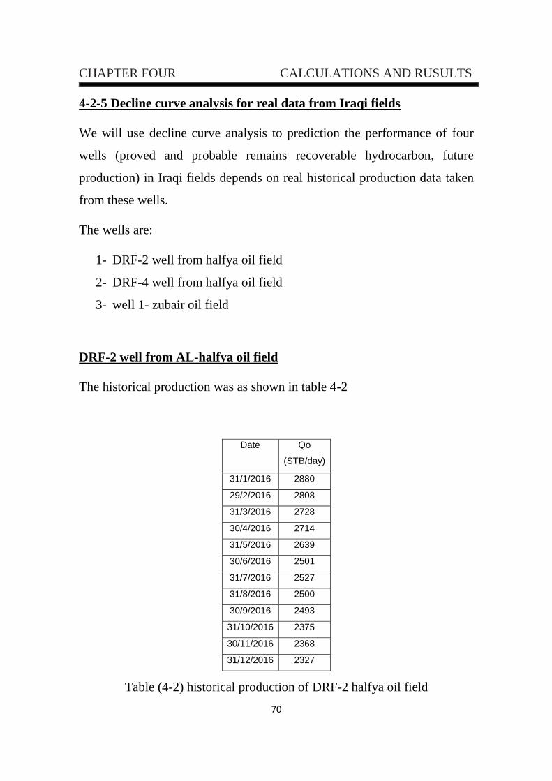
70
CHAPTER FOUR CALCULATIONS AND RUSULTS
4-2-5 Decline curve analysis for real data from Iraqi fields
We will use decline curve analysis to prediction the performance of four
wells (proved and probable remains recoverable hydrocarbon, future
production) in Iraqi fields depends on real historical production data taken
from these wells.
The wells are:
1- DRF-2 well from halfya oil field
2- DRF-4 well from halfya oil field
3- well 1- zubair oil field
DRF-2 well from AL-halfya oil field
The historical production was as shown in table 4-2
Date Qo
(STB/day)
31/1/2016 2880
29/2/2016 2808
31/3/2016 2728
30/4/2016 2714
31/5/2016 2639
30/6/2016 2501
31/7/2016 2527
31/8/2016 2500
30/9/2016 2493
31/10/2016 2375
30/11/2016 2368
31/12/2016 2327
Table (4-2) historical production of DRF-2 halfya oil field
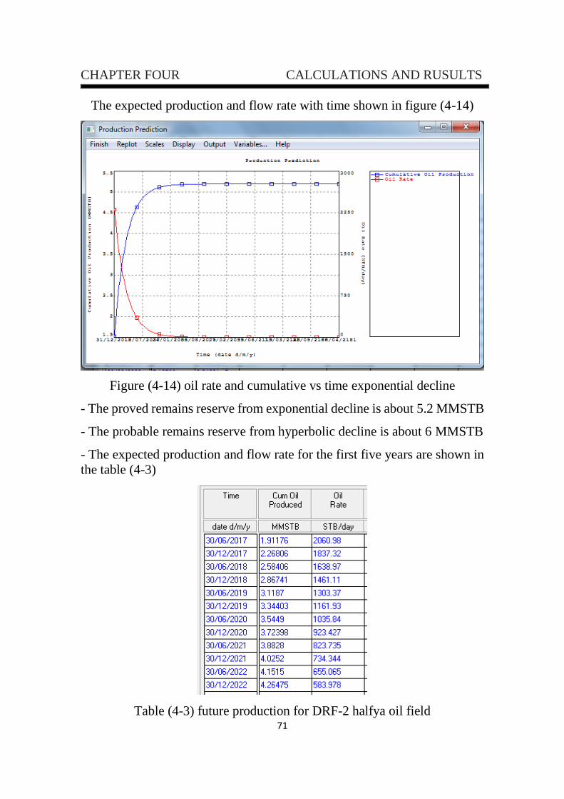
71
CHAPTER FOUR CALCULATIONS AND RUSULTS
The expected production and flow rate with time shown in figure (4-14)
Figure (4-14) oil rate and cumulative vs time exponential decline
- The proved remains reserve from exponential decline is about 5.2 MMSTB
- The probable remains reserve from hyperbolic decline is about 6 MMSTB
- The expected production and flow rate for the first five years are shown in
the table (4-3)
Table (4-3) future production for DRF-2 halfya oil field
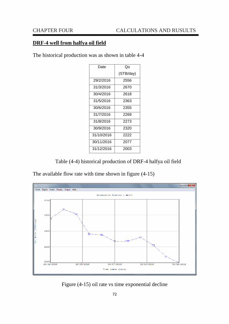
72
CHAPTER FOUR CALCULATIONS AND RUSULTS
DRF-4 well from halfya oil field
The historical production was as shown in table 4-4
Date Qo
(STB/day)
29/2/2016 2556
31/3/2016 2670
30/4/2016 2618
31/5/2016 2363
30/6/2016 2355
31/7/2016 2269
31/8/2016 2273
30/9/2016 2320
31/10/2016 2222
30/11/2016 2077
31/12/2016 2003
Table (4-4) historical production of DRF-4 halfya oil field
The available flow rate with time shown in figure (4-15)
Figure (4-15) oil rate vs time exponential decline
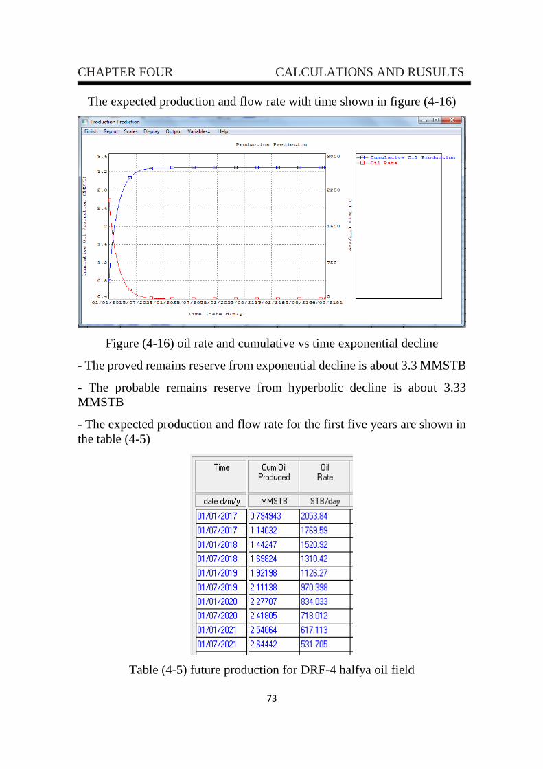
73
CHAPTER FOUR CALCULATIONS AND RUSULTS
The expected production and flow rate with time shown in figure (4-16)
Figure (4-16) oil rate and cumulative vs time exponential decline
- The proved remains reserve from exponential decline is about 3.3 MMSTB
- The probable remains reserve from hyperbolic decline is about 3.33
MMSTB
- The expected production and flow rate for the first five years are shown in
the table (4-5)
Table (4-5) future production for DRF-4 halfya oil field
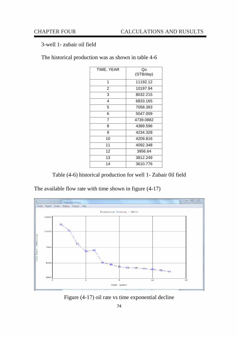
74
CHAPTER FOUR CALCULATIONS AND RUSULTS
3-well 1- zubair oil field
The historical production was as shown in table 4-6
TIME, YEAR Qo (STB/day)
1 11192.12
2 10197.94
3 8032.215
4 6833.165
5 7058.393
6 5047.009
7 4739.0882
8 4389.596
9 4234.328
10 4209.816
11 4092.348
12 3956.64
13 3812.249
14 3610.776
Table (4-6) historical production for well 1- Zubair 0il field
The available flow rate with time shown in figure (4-17)
Figure (4-17) oil rate vs time exponential decline
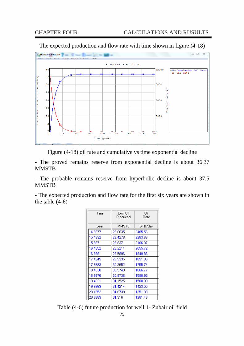
75
CHAPTER FOUR CALCULATIONS AND RUSULTS
The expected production and flow rate with time shown in figure (4-18)
Figure (4-18) oil rate and cumulative vs time exponential decline
- The proved remains reserve from exponential decline is about 36.37
MMSTB
- The probable remains reserve from hyperbolic decline is about 37.5
MMSTB
- The expected production and flow rate for the first six years are shown in
the table (4-6)
Table (4-6) future production for well 1- Zubair oil field

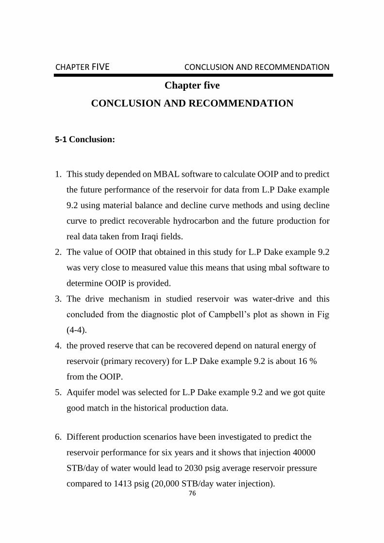
76
CHAPTER FIVE CONCLUSION AND RECOMMENDATION
Chapter five
CONCLUSION AND RECOMMENDATION
5-1 Conclusion:
1. This study depended on MBAL software to calculate OOIP and to predict
the future performance of the reservoir for data from L.P Dake example
9.2 using material balance and decline curve methods and using decline
curve to predict recoverable hydrocarbon and the future production for
real data taken from Iraqi fields.
2. The value of OOIP that obtained in this study for L.P Dake example 9.2
was very close to measured value this means that using mbal software to
determine OOIP is provided.
3. The drive mechanism in studied reservoir was water-drive and this
concluded from the diagnostic plot of Campbell’s plot as shown in Fig
(4-4).
4. the proved reserve that can be recovered depend on natural energy of
reservoir (primary recovery) for L.P Dake example 9.2 is about 16 %
from the OOIP.
5. Aquifer model was selected for L.P Dake example 9.2 and we got quite
good match in the historical production data.
6. Different production scenarios have been investigated to predict the
reservoir performance for six years and it shows that injection 40000
STB/day of water would lead to 2030 psig average reservoir pressure
compared to 1413 psig (20,000 STB/day water injection).
77
CHAPTER FIVE CONCLUSION AND RECOMMENDATION
7. Water injection can be used to reduce drop pressure of reservoir (first
case) also it can be used to increase life of reservoir (second case).
8. The decline curve analysis used for wells from real data provide us with
a satisfied and quick results in calculating the oil remaining reserves and
future production from past production information.
9. There are different types of decline curve which will depend upon the
past production of the field or well in order to be taken in account when
preformation calculations the exponential decline gives the proved
reserve while hyperbolic decline gives probable reserve.
10. We use decline curve analysis for two wells from alhalfya oil field and
well number one from zubair oil field.
11. The decline curve will find the economic limit line at some time. That
will be is the end of oilfield production life, conditioned by present
technology, production cost, contracts and state regulations.
5.2. Recommendations
1. MBAL software is good and reliable software in calculating OOIP and
predicting the performance of the reservoir in the future.
2. MBAL software has many tools like material balance and decline curve
so it's very suitable to predict the performance of reservoir.
3. Softwares such as: Petrel and Eclipse can be used to make sure that the
results obtained from MBAL are valid results.
4. PVT data can be calculated by another software like PVTP software to
take in consideration of multi well PVT.
78
Reference
1. Ahmed T. (2000) Reservoir engineering handbook, Houston (TX), Gulf.
2. Craft.B., Hawkins.M., revised by Terry.R.(1991) Applie Petroleum
Reservoir Engineering, Second Edition, Prentice – Hall Inc.Eaglewood
Cliffs, NJ 56-65.
3. Dake.L.(1994) The Practice of Reservoir Engineering, Elsevier,
Amsterdam, NJ
4. M.Abu El Ela. (2007) “Reservoir Characterization from Material Balance
result analysis paper SPE 108648 presented at the SPE International Oil
Conference and Exhibition held in Veracruz, Mexico.
5. Standing M. B (1997), Volumetric and Phase Behavior of Oil Field
Hydrocarbon System, PP. 125-126 Dallas: Society of Petroleum Engineers
6. Pletcher. J.L (2002) “Improvements to Reservoir Material Balance
Methods”, paper SPE 75354, presented at the SPE Annual Technical
Conference and Exhibition held in Dallas.
7. Glaso,O., (1980): "Generalized Pressure Volume-Temperature
Correlations", May, Pp. 785-795
8. Fetkovich, M. J, (1971): "A Simplified Approach to Water Influx
Calculations- Finite Aquifer Systems," JPT, PP. 814-828
9. Petroleum experts, mbal, handtoolit, version 8.1, December 2005.
10. Havlena, D., and odeh, A. S.] (1963): ''Balance as an Equation of a
Straight Line", Trans, AlME, Part 1: 228 I-H96; Part 2: 231 I 815
11. Baker.R.(2003) “PVT Error Analysis for Material Balance
Calculation”.Paper presented at the Canadian International Petroleum
Conference, Calgary, Alberta.
12.Arps, J.J.: “Analysis of Decline Curves,” Trans. AIME, 160, 228-247,
1945.
13.Fetkovich, E. J., Fetkovich, M. J., and Fetkovich, M. D., “Useful
Concepts for Decline Curve Forecasting, Reserve Estimation, and Analysis,
Reservoir Engineering, February 1996.
14. http://www.fekete.com/software/rta/media/webhelp/c-te-analysis.htm
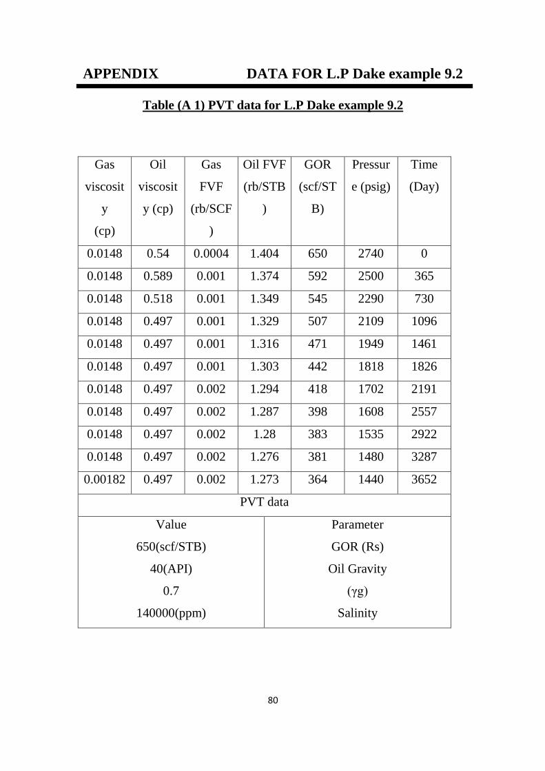
80
APPENDIX DATA FOR L.P Dake example 9.2
Table (A 1) PVT data for L.P Dake example 9.2
Time
(Day)
Pressur
e (psig)
GOR
(scf/ST
B)
Oil FVF
(rb/STB
)
Gas
FVF
(rb/SCF
)
Oil
viscosit
y (cp)
Gas
viscosit
y
(cp)
0 2740 650 1.404 0.0004 0.54 0.0148
365 2500 592 1.374 0.001 0.589 0.0148
730 2290 545 1.349 0.001 0.518 0.0148
1096 2109 507 1.329 0.001 0.497 0.0148
1461 1949 471 1.316 0.001 0.497 0.0148
1826 1818 442 1.303 0.001 0.497 0.0148
2191 1702 418 1.294 0.002 0.497 0.0148
2557 1608 398 1.287 0.002 0.497 0.0148
2922 1535 383 1.28 0.002 0.497 0.0148
3287 1480 381 1.276 0.002 0.497 0.0148
3652 1440 364 1.273 0.002 0.497 0.00182
PVT data
Parameter
GOR (Rs)
Oil Gravity
(γg)
Salinity
Value
650(scf/STB)
40(API)
0.7
140000(ppm)
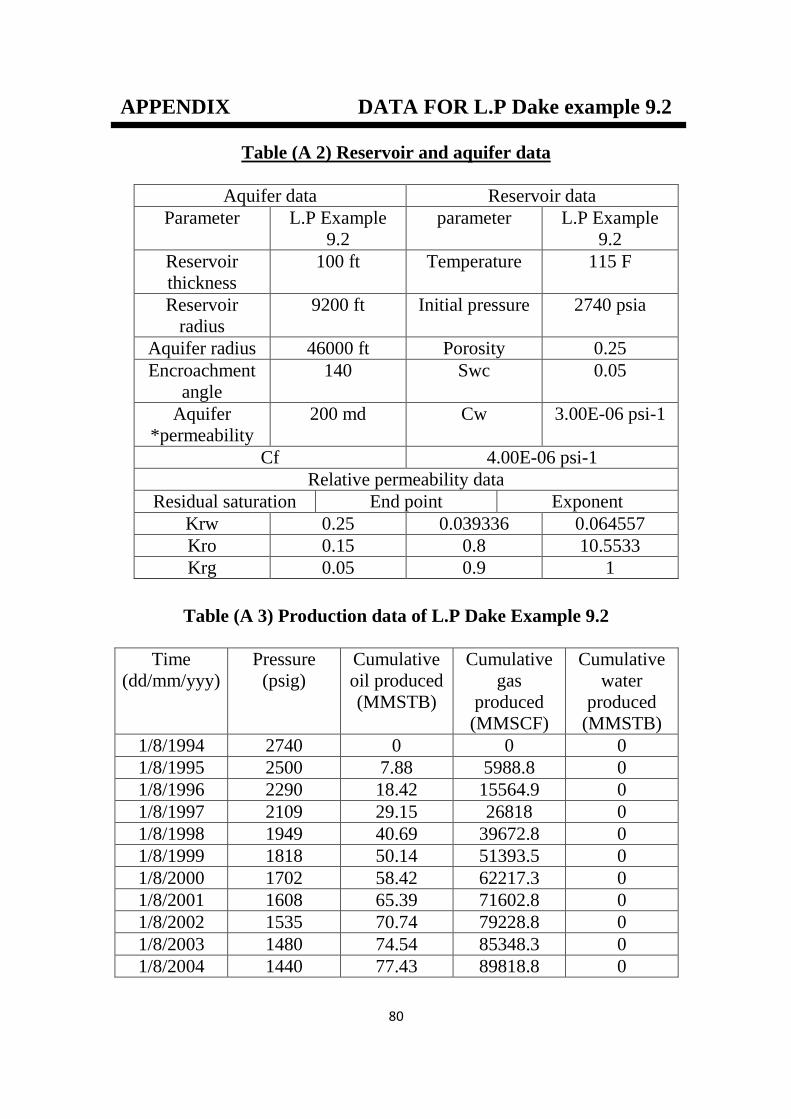
80
APPENDIX DATA FOR L.P Dake example 9.2
Table (A 2) Reservoir and aquifer data
Reservoir data Aquifer data
L.P Example
9.2
parameter L.P Example
9.2
Parameter
115 F Temperature 100 ft Reservoir
thickness
2740 psia Initial pressure 9200 ft Reservoir
radius
0.25 Porosity 46000 ft Aquifer radius
0.05 Swc 140 Encroachment
angle
3.00E-06 psi-1 Cw 200 md Aquifer
*permeability
4.00E-06 psi-1 Cf
Relative permeability data
Exponent End point Residual saturation
0.064557 0.039336 0.25 Krw
10.5533 0.8 0.15 Kro
1 0.9 0.05 Krg
Table (A 3) Production data of L.P Dake Example 9.2
Cumulative
water
produced
(MMSTB)
Cumulative
gas
produced
(MMSCF)
Cumulative
oil produced
(MMSTB)
Pressure
(psig)
Time
(dd/mm/yyy)
0 0 0 2740 1/8/1994
0 5988.8 7.88 2500 1/8/1995
0 15564.9 18.42 2290 1/8/1996
0 26818 29.15 2109 1/8/1997
0 39672.8 40.69 1949 1/8/1998
0 51393.5 50.14 1818 1/8/1999
0 62217.3 58.42 1702 1/8/2000
0 71602.8 65.39 1608 1/8/2001
0 79228.8 70.74 1535 1/8/2002
0 85348.3 74.54 1480 1/8/2003
0 89818.8 77.43 1440 1/8/2004


![Prediction of Reservoir Performance Applying Decline Curve ... · Decline curve analysis is the most currently method used available and sufficient [1].The most popular decline curve](https://img.pdfslide.us/doc/110x75/5eb99c14e247933c8377a1f7/prediction-of-reservoir-performance-applying-decline-curve-decline-curve-analysis.jpg)