Embed Size (px)
Citation preview
1
DRAFT
Probabilistic Decline Curve Analysis of Barnett, Fayetteville, Haynesville, and
Woodford Gas Shales
J. R. Fanchi, M. J. Cooksey, K. M. Lehman and A. Smith
Department of Engineering and Energy Institute
Texas Christian University
and
A.C. Fanchi and C. J. Fanchi
Energy.Fanchi.com
June 25, 2013
Abstract
This paper presents a probabilistic decline curve workflow to model shale gas
production from the Barnett, Fayetteville, Haynesville, and Woodford shales. Ranges of
model input parameters for four gas shales are provided to guide the preparation of
uniform and triangle probability distributions. The input parameter ranges represent
realistic distributions of model parameters for specific gas shales.
Keywords: Shale Gas; Decline Curve Analysis; Monte Carlo Analysis; Probability
Distributions

2
1. Introduction
Many people have developed techniques that were designed to forecast
production from unconventional resources, such as Brown, et al. (2009), Valkó and Lee
(2010), Duong (2011), Anderson, et al. (2012), and Esmaili, et al. (2012). Our ability to
forecast shale gas production is complicated by our inability to correctly account for all
of the mechanisms that affect production. We present a probabilistic workflow that is a
modification of reservoir simulation workflows and is designed for use with rate-time
decline curve models.
Different workflows exist for performing reservoir simulation projects. For
example, Fanchi has presented workflows for green fields (Fanchi, 2010 and 2011a) and
brown fields (Fanchi, 2010 and 2011b) that use reservoir flow models to generate a
distribution of recovery forecasts. The workflows are able to integrate uncertainty in the
development of recovery forecasts. The workflow presented here uses the probabilistic
decline curve analysis (DCA) workflow to develop model input parameter ranges for the
Barnett, Fayetteville, Haynesville, and Woodford shales. The methodology is automated
in the form of a software program that calculates the distribution of Estimated Ultimate
Recovery (EUR) for production of gas from unconventional gas shale. Using well data
from different shale gas plays, we determined realistic minimum and maximum values
for the uniform distribution of a parameter and triangular distribution of a parameter. The
realistic ranges of model input parameters can be used to guide the preparation of
uniform and triangle probability distributions.
3
2. Decline Curve Models for Unconventional Resources
Decline curve models used here must have finite, bounded values of EUR. Not all
decline curve models satisfy this criterion. For example, Arps (1945) presented the
following empirical decline curve model for flow rate q as a function of time t and
parameters a, b:
1 baqdt
dq (1)
The Arps models are harmonic decline (b = 1), exponential decline (b = 0), and
hyperbolic decline with other positive values of b. The hyperbolic model typically has b
< 1 for conventional reservoir production. The Arps harmonic model (b = 1) and
hyperbolic model with b > 1 are not always applicable to unconventional reservoir
production forecasts because extrapolation of the decline curve can lead to unbounded
values of EUR and corresponding overestimates of EUR.
The Arps exponential model does not always adequately model the decline rate of
unconventional reservoir production. Valkó and Lee (2010) introduced the Stretched
Exponential Decline Model (SEDM) as a generalization of the Arps exponential model.
The SEDM is based on the idea that several decaying systems comprise a single decaying
system (Phillips, 1996; and Johnston, 2006). If we think of production from a reservoir as
a collection of decaying systems in a single decaying system, then SEDM can be viewed
as a model of the decline in flow rate. The SEDM has three parameters qi, n and τ (or a,
b, c):
] )exp[-(t/ a= ] )exp[-(t/ q=q cn
i b (2)
4
Parameter qi is flow rate at initial time t. The Arps exponential decline model is the
special case of SEDM with n = 1.
A second decline curve model is based on the logarithmic relationship between
pressure and time in a radial flow system. We can use productivity index to link rate and
pressure to obtain the logarithmic decline curve model
b+lnt a=q (3)
with parameters a and b. This logarithm model is referred to as the LNDM model.
The third decline curve model used here is the Arps hyperbolic decline curve
model with the restriction that 0 < b < 1. The hyperbolic model
(-1/b)bct)+a(1=q (4)
is referred to as the HYDM model.
Model input parameters for each decline curve model are summarized in Table 1.
Cumulative gas production Q is given by the integral
T
T0
dtq=Q (5)
The lower limit T0 is the initial time and the upper limit T is the time when the economic
limit is reached.
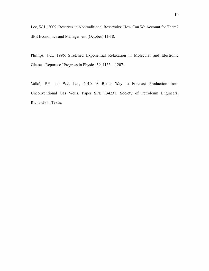
3. Probabilistic DCA Workflow
Reserves estimates may be either deterministic or probabilistic (Lee, 2009). A
deterministic estimate of reserves is a single best estimate of reserves based on
geological, engineering, and economic data. A probabilistic estimate of reserves uses
geological, engineering, and economic data to generate a range of estimates and their
5
associated probabilities. Linear regression can be used to obtain a deterministic estimate
of reserves. The probabilistic estimate of reserves is obtained here using the workflow for
probabilistic DCA of unconventional gas production outlined in Figure 1.
Each step of the probabilistic decline curve analysis method is briefly described
below. More discussion can be found in Fanchi (2012a, 2012b).
Step DCA1: Gather Rate-Time Data
Acquire production rate as a function of time. Remove significant shut-in periods
so rate-time data represents continuous production.
Step DCA2: Select a DCA Model and Specify Input Parameter Distributions
The number of input parameters depends on the DCA model chosen. The SEDM
model requires three parameters, and the LNDM model requires two parameters.
Parameter distributions may be either uniform or triangle distributions.
Step DCA3: Specify Constraints
Available rate-time production history is used to decide which DCA trials are
acceptable. Every DCA model run that uses a complete set of model input parameters
constitutes a trial. The results of each trial are then compared to user-specified criteria.
Criteria options include an objective function, rate at the end of history, and cumulative
6
production at the end of history. The objective function quantifies the quality of the
match by comparing the difference between model rates and observed rates. Objective
functions with smaller values are considered better matches than objective functions with
larger values.
Step DCA4: Generate Decline Curve Trials
Decline curve trials are obtained by running the DCA model. The number of trials is
specified by the analyst.
Step DCA5: Determine Subset of Acceptable Trials
The trials generated in Step DCA4 are compared to the criteria specified in Step DCA3.
Each trial that satisfies the user-specified criteria is included in a subset of acceptable
trials.
Step DCA6: Generate Distribution of Performance Results
The distribution of EUR values for the subset of acceptable trials is analyzed and the 10th
(PC10), 50th (PC50), and 90th (PC90) percentiles are determined.
4. Model Results
7
The workflow in Figure 1 is applied using rate-time data for gas production for a
sampling of wells from the Barnett (30 wells), Fayetteville (10 wells), Haynesville (10
wells), and Woodford shales (60 wells). Three DCA models (SEDM, LNDM, and
HYDM) are used to match rate-time data for each well. The Monte Carlo analysis uses
1000 trials initially. The value of parameter b in the HYDM model is restricted to the
range 0.01 < b < 0.99. A match of cumulative gas production at the end of the historical
production period is used as the constraint for selecting the subset of trials. The constraint
requires that the decline curve model and its set of model parameters must generate a
cumulative gas production that matches actual cumulative gas production to within 1%
by the end of the historical production period.
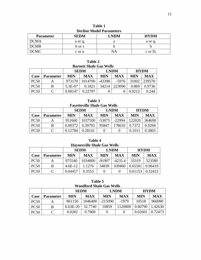
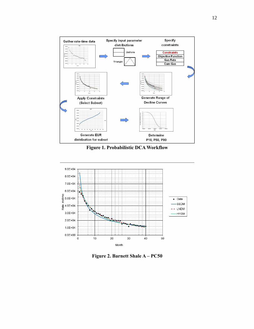
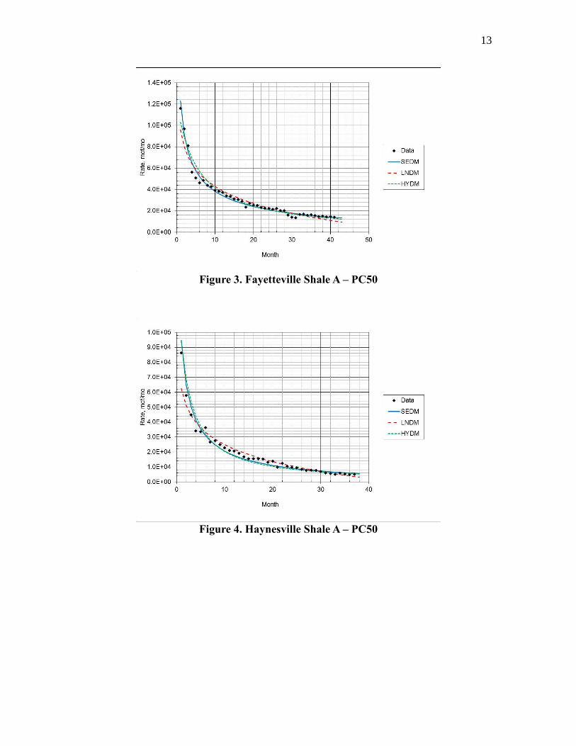
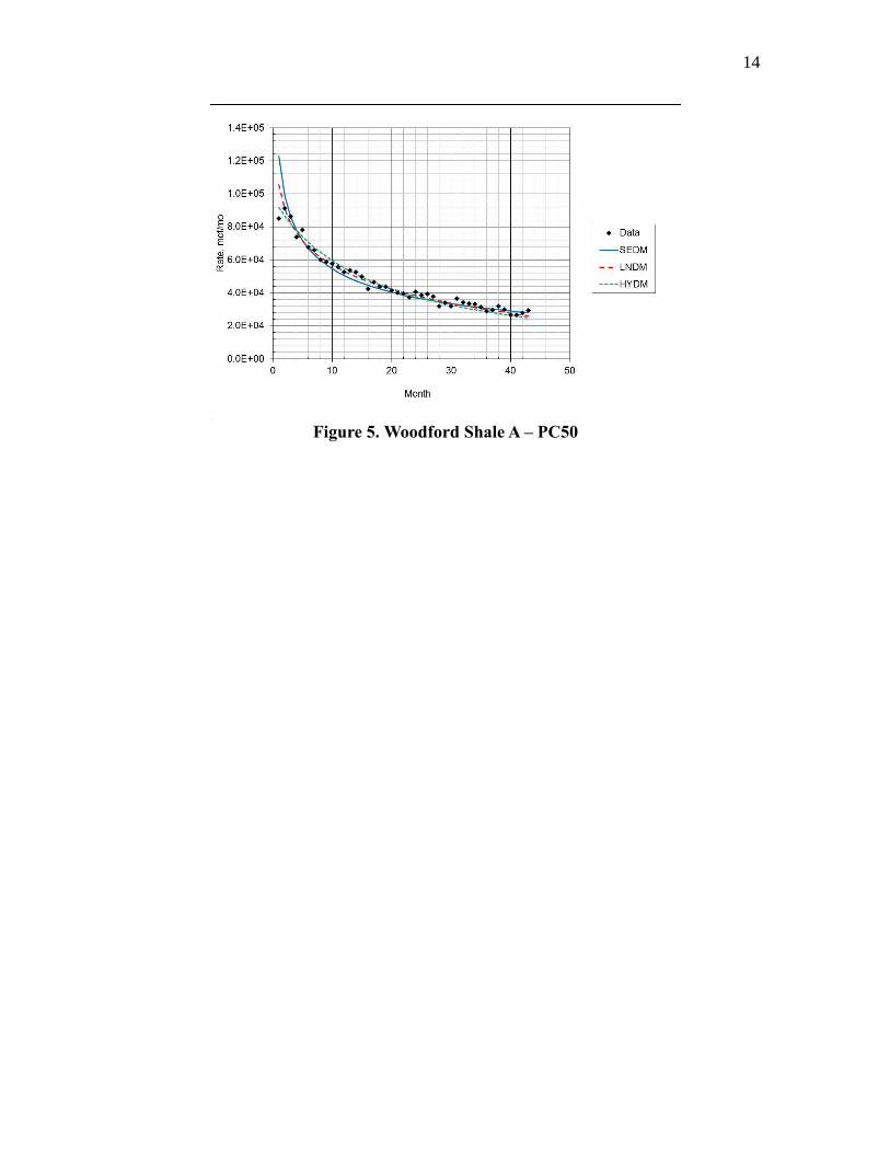
Figures 2 through 5 illustrate the quality of the matches for each shale gas play.
Each figure shows the match of the 50th
percentile (PC50) trial to well data. The
parameters for the PC50 trial are collected and a minimum and maximum value for each
model parameter is determined for the set of wells in each play. Model trials that do not
satisfy the cumulative gas constraint are not used to determine minimum and maximum
model input parameter values.
Tables 2 through 5 present minimum and maximum values for parameters of each
decline curve model.
5. Concluding Remarks
We have analyzed shale gas production from the Barnett, Fayetteville,
Haynesville, and Woodford shales using a probabilistic decline curve workflow.
8
Minimum and maximum values of model input parameters were determined from the
model input parameters for the 50th
percentile trials. The model input parameter ranges
are realistic distributions of model parameters that can be used to guide the preparation of
uniform and triangle probability distributions.
Acknowledgement
We thank drillinginfo.com for access to their database of well production data.
References
Anderson, D.M., P. Liang, and V. Okouma, 2012. Probabilistic Forecasting of
Unconventional Resources Using Rate Transient Analysis: Case Studies. Paper SPE
155737. Society of Petroleum Engineers, Richardson, Texas.
Arps, J.J., 1945. Analysis of Decline Curves. Paper SPE 945228-G. Trans. AIME,
Volume 160, 228-247.
Brown, M., E. Ozkan, R. Raghavan, and H. Kazemi, 2009. Practical Solutions for
Pressure Transient Responses of Fractured Horizontal Wells in Unconventional
Reservoirs. Paper SPE 125043. Society of Petroleum Engineers, Richardson, Texas.
Duong, A.N, 2011. Rate-Decline Analysis for Fracture-Dominated Shale Reservoirs, SPE
Reservoir Evaluation and Engineering (June) 377-387.
9
Esmaili, S., A. Kalantari-Dahegi, and S.D. Mohaghegh, 2012. Forecasting, Sensitivity
and Economic Analysis of Hydrocarbon Production from Shale Plays using Artificial
Intelligence and Data Mining. Paper SPE 162700. Society of Petroleum Engineers,
Richardson, Texas.
Fanchi, J.R., 2010. Integrated Reservoir Asset Management. Elsevier-Gulf Professional
Publishing, Burlington, Massachusetts.
Fanchi, J.R., 2011a. Flow Modeling Workflow: I. Green Fields, Journal of Petroleum
Science and Engineering Volume 79, 54–57.
Fanchi, J.R., 2011b. Flow Modeling Workflow: II. Brown Fields, Journal of Petroleum
Science and Engineering Volume 79, 58–63.
Fanchi, J.R., 2012 a. Forecasting Shale Gas Recovery Using Monte Carlo Analysis – Part
1, on PennEnergy.com, PennWell publishing; accessed online Dec. 3, 2012
Fanchi, J.R., 2012 b. Forecasting Shale Gas Recovery Using Monte Carlo Analysis – Part
2, on PennEnergy.com, PennWell publishing; accessed online Dec. 5, 2012
Johnston, D.C., 2006. Stretched Exponential Relaxation Arising from a Continuous Sum
of Exponential Decays. Physical Review B 74: 184430.
10
Lee, W.J., 2009. Reserves in Nontraditional Reservoirs: How Can We Account for Them?
SPE Economics and Management (October) 11-18.
Phillips, J.C., 1996. Stretched Exponential Relaxation in Molecular and Electronic
Glasses. Reports of Progress in Physics 59, 1133 – 1207.
Valkó, P.P. and W.J. Lee, 2010. A Better Way to Forecast Production from
Unconventional Gas Wells. Paper SPE 134231. Society of Petroleum Engineers,
Richardson, Texas.
11
Table 1
Decline Model Parameters
Parameter SEDM LNDM HYDM
DCMA a or qi a a or qi
DCMB b or τ b b
DCMC c or n NA c or Di
Table 2
Barnett Shale Gas Wells
SEDM LNDM HYDM
Case Parameter MIN MAX MIN MAX MIN MAX
PC50 A 973170 1014700 -43398 -5976 31002 239570
PC50 B 5.3E-07 0.1821 34214 223090 0.869 0.9736
PC50 C 0.08147 0.22797 0 0 0.0212 0.244
Table 3
Fayetteville Shale Gas Wells
SEDM LNDM HYDM
Case Parameter MIN MAX MIN MAX MIN MAX
PC50 A 951660 1037500 -53075 -22994 122020 364690
PC50 B 0.00372 0.39793 95847 178610 0.7372 0.9294
PC50 C 0.12784 0.28141 0 0 0.1011 0.3803
Table 4
Haynesville Shale Gas Wells
SEDM LNDM HYDM
Case Parameter MIN MAX MIN MAX MIN MAX
PC50 A 975540 1034800 -91907 -4235.4 33319 523580
PC50 B 4.6E-12 1.1276 34839 339460 0.65501 0.96419
PC50 C 0.04457 0.3553 0 0 0.01153 0.52415
Table 5
Woodford Shale Gas Wells
SEDM LNDM HYDM
Case Parameter MIN MAX MIN MAX MIN MAX
PC50 A 961150 1046400 -215090 -1979 10518 966990
PC50 B 6.63E-20 32.7740 10859 1120800 0.60790 1.42630
PC50 C 0.0282 0.7969 0 0 0.02601 0.72473
12
Figure 1. Probabilistic DCA Workflow
Figure 2. Barnett Shale A – PC50
13
Figure 3. Fayetteville Shale A – PC50
Figure 4. Haynesville Shale A – PC50
14
Figure 5. Woodford Shale A – PC50