RELIABILITY-BASED MAINTENANCE OPTIMIZATION OF WALKING

DRAGLINES

A THESIS SUBMITTED TO

THE GRADUATE SCHOOL OF NATURAL AND APPLIED SCIENCES

OF

MIDDLE EAST TECHNICAL UNIVERSITY

BY

ONUR GÖLBAŞI

IN PARTIAL FULLFILMENT OF THE REQUIREMENTS

FOR

THE DEGREE OF DOCTOR OF PHILOSOPHY

IN

MINING ENGINEERING

SEPTEMBER 2015

Approval of the thesis:

RELIABILITY-BASED MAINTENANCE OPTIMIZATION OF WALKING

DRAGLINES

submitted by ONUR GÖLBAŞI in partial fulfillment of the requirements for the

degree of Doctor of Philosophy in Mining Engineering Department, Middle East

Technical University by,

Prof. Dr. Gülbin Dural Ünver .

Dean, Graduate School of Natural and Applied Science

Prof. Dr. Ali İhsan Arol .

Head of Department, Mining Engineering

Assoc. Prof. Dr. Nuray Demirel .

Supervisor, Mining Engineering Dept., METU

Examining Committee Members:

Prof. Dr. Bahtiyar Ünver _____________________

Mining Engineering Dept., HU

Assoc. Prof. Dr. Nuray Demirel _____________________

Mining Engineering Dept., METU

Prof. Dr. H. Şebnem Düzgün _____________________

Mining Engineering Dept., METU

Assoc. Prof. Dr. Sevtap Kestel _____________________

Institute of Applied Mathematics, METU

Assoc. Prof. Dr. Mehmet Ali Hindistan _____________________

Mining Engineering Dept., HU

Date: 10.09.2015

I hereby declare that all information in this document has been obtained and

presented in accordance with academic rules and ethical conduct. I also declare

that, as required by these rules and conduct, I have fully cited and referenced all

material and results that are not original to this work.

Name, Last Name: Onur Gölbaşı

Signature:

v

ABSTRACT

RELIABILITY-BASED MAINTENANCE OPTIMIZATION OF WALKING

DRAGLINES

Gölbaşı, Onur

Ph.D., Mining Engineering Department

Advisor: Assoc. Prof. Dr. Nuray Demirel

September 2015, 187 pages

Dragline is an earthmover extensively utilized in open cast coal mines for overburden

stripping activities. Since the machinery breakdowns may induce high amount of

production losses, draglines are required to be operated with high availability. In this

sense, effective maintenance policies are essential to improve longevity of dragline

component and sustainability of operations. In this research study, it is aimed to

develop a reliability-based maintenance optimization models for two walking

draglines, Page and Marion, currently operated in Tunçbilek coal mine. The study

methodology consists of four main phases as: i) characterizing the machinery

components via reliability models, ii) implementing a decision platform for preventive

replacement of components, iii) generating risk-based maintenance importance models

for the machinery components, and iv) developing an optimization algorithm for

inspection intervals of the draglines. Component and system characterization was

achieved generating deductive reliability models. Preventive component replacement

models were created considering preventive and corrective cost factors and

investigating applicability of preventive replacements for components. Risk model

was developed regarding indirect and direct maintenance costs and maintenance

criticality scores were estimated for system elements. Optimization algorithm on

inspection intervals was implemented including random lifetime and repair behaviors

of components, functional effect of each other during failures, scheduled halts in shifts

and regular inspections, and direct and indirect costs of maintenance activities.

vi

The results of reliability models revealed that dragging and bucket units were expected

to fail most frequently. On the other hand, boom unit was detected to sustain its

functionality for the longest time compared to the other units. Moreover, machinery

house components generally lead to the longest repairing time and the highest

production loss. Considering individual components and their associated structural and

functional dependencies, Marion and Page draglines are expected to keep operation

going for 34.04 and 35.62 hours without any breakdown, respectively. In addition,

optimization algorithm for inspection intervals showed that interval lengths of 184 and

232 hours are economically optimal for Page and Marion, respectively. Maintenance

costs of the draglines using these intervals are expected to decrease with 5.9% for Page

and 6.2% for Marion. Moreover, risk-based reliability allocation models showed that

reliability improvement in motor, generator, rotation, and walking had the greatest

impact on overall system reliability considering failure frequencies and their

consequences. It was revealed from the risk model that maintenance for these

components should be carried out in more controlled and planned manner. This

research study provides a new perspective on dragline maintenance. The main novelty

and expected industrial contribution of this study is to provide a new inspection

optimization model and implementation of risk factors to identify draglines’

component maintenance criticality considering reliability allocation which has not

been considered previously in literature.

Keywords: Dragline, reliability, maintenance optimization, age-replacement policy,

risk model, inspection interval optimization.

vii

ÖZ

YÜRÜYEN ÇEKME KEPÇELİ YERKAZARLARIN GÜVENİLİRLİK TABANLI

BAKIM-ONARIM OPTİMİZASYONU

Gölbaşı, Onur

Doktora, Maden Mühendisliği Bölümü

Tez Yöneticisi: Doç. Dr. Nuray Demirel

Eylül 2015, 187 sayfa

Çekme kepçeli yerkazarlar, açık kömür ocaklarında örtü kazı dekapajı için sıklıkla

kullanılan yerkazarlardır. Makine duraksamaları yüksek miktarda üretim kaybına

neden olacağından, çekme kepçeli yerkazarların yüksek kullanılabilirlik oranıyla

çalıştırılmaları gerekmektedir. Bu bakımdan, etkili bakım onarım politikaları, çekme

kepçe parçalarının uzun ömürlü olarak kullanılması ve operasyonların

sürdürülebilirliği için gereklidir. Bu çalışmada, Tunçbilek açık kömür işletmesinde

kullanılan Page ve Marion marka iki farklı yerkazar için güvenilirlik tabanlı bakım

onarım optimizasyonunun yapılması amaçlamaktadır. Çalışma metodolojisi dört ana

aşamadan oluşmaktadır. Bunlar: i) Makine parçalarının güvenilirlik modelleriyle

yaşam özelliklerinin belirlenmesi, ii) Önleyici parça değişimleri için bir karar

platformunun oluşturulması, iii) Makine parçaları için risk tabanlı bakım onarım

önemi modelinin kurulması ve iv) Çekme kepçeli yerkazarların düzenli denetim

aralıkları için bir optimizasyon algoritması geliştirilmesidir. Bileşen ve sistem

karakterizasyonu, tümdengelimli güvenilirlik modelleri oluşturularak elde edilmiştir.

Önleyici parça değişim modelleri, önleyici ve düzeltici bakım masraflarını hesaba

katılarak ve parçaların önleyici değişim uygulanabilirliğini incelenerek

oluşturulmuştur. Risk modeli, arıza neticesinde oluşan doğrudan ve dolaylı maliyetler

hesaba katılarak geliştirilmiş ve sistem elemanları için bakım-onarım öncelik

sıralaması tahmin edilmiştir. Denetim aralığına dair optimizasyon algoritması,

viii

bileşenlerin rasgele yaşam ve onarım davranışları, arızalar sırasında her bir parçanın

birbirine fonksiyonel etkisi, vardiya değişimleri ve düzenli denetimlerden kaynaklı

zorunlu duraksamalar ve bakım onarım aktivitelerinin neden olduğu doğrudan ve

dolaylı tüm maliyetler hesaba katılarak gerçekleştirilmiştir.

Güvenilirlik modellerinin sonuçları, kepçe ve çekiş ünitelerinin en sık arızalanan

üniteler olduğunu göstermiştir. Diğer yandan, bum ünitesinin diğer ünitelerle

karşılaştırıldığında en uzun süre işlevselliğini devam ettirdiği tespit edilmiştir. Ek

olarak, makina dairesi bileşenleri genellikle en uzun süreli onarım sürelerine ve en

yüksek üretim kaybına neden olmaktadır. Bireysel bileşenler, onlar arasındaki yapısal

ve fonksiyonel bağımlılıklar düşünüldüğünde, Marion ve Page çekme kepçelerinin

sırasıyla 34,04 ve 35,62 saat boyunca herhangi bir bozulma yaşamadan

operasyonlarına devam etmeleri beklenmektedir. Ayrıca, denetim aralıkları için

oluşturulan optimizasyon algoritması, Page ve Marion için 184 ve 232 saatlik denetim

aralıklarının ekonomik olarak optimal olacağını göstermektedir. Bu aralıklar

kullanılarak, çekme kepçelerin bakım-onarım masraflarında Page için %6,2, Marion

için %5,9 oranında bir düşüş olması beklenilebilir. Bunlara ek olarak, risk-tabanlı

güvenilirlik paylaştırma modelleri, arıza aralıkları ve arıza sonuçlarına göre, motor,

jeneratör, dönme ve yürüme mekanizmalarındaki güvenilirlik artışının sistem

güvenilirliğine en yüksek katkıyı sağlayacağını göstermektedir. Bu parçalara yönelik

bakımın, daha planlı ve kontrollü yapılması gerektiği anlaşılmıştır. Bu araştırma,

çekme kepçeli yerkazarların bakım onarımına yeni bir bakış açısı sağlamaktadır.

Çalışmanın literatüre ve endüstriye kazandıracağı en önemli yenilik, güvenilirlik

dağılımı yolu ile çekme kepçeli yer kazarların bileşenlerinin bakım onarım öncelik

sıralamasının tahmin edilmesi için risk faktörlerinin belirlenerek yeni bir bakım-

denetim optimizasyonu modelinin geliştirilmesidir.

Anahtar Kelimeler: Çekme kepçeli yerkazar, bakım-onarım optimizasyonu, yaş-

tabanlı parça değişim politikaları, risk modeli, denetim aralıklarının optimizasyonu.

ix

ACKNOWLEDGEMENTS

First and foremost, I would like to express my deepest gratitude to my supervisor,

Assoc. Prof. Dr. Nuray Demirel for her support, guidance, and suggestions in this

thesis research. Without her patience and encouragement, this thesis would not have

been completed. I also would like to extend my sincere appreciations to the members

of examining committee, Prof. Dr. H. Şebnem Düzgün, Prof. Dr. Bahtiyar Ünver,

Assoc. Prof. Dr. Sevtap Kestel, and Assoc. Prof. Dr. Mehmet Ali Hindistan for their

constructive criticism and suggestions for the thesis.

I would like to thank The Scientific and Technological Research Council of Turkey

(Project No: 111M320) for supporting this research.

I owe a particular gratitude to Metin Özdoğan, Enver Şekerci, and employees of

Tunçbilek coal mine for their helps and providing information about the draglines.

Their ideas and comments have been quite helpful in my doctoral thesis.

I would also like to thank to my colleagues for their moral supports and

encouragements. I cannot forget their motivations and helps throughout my PhD

process. I feel indebted especially to Deniz Tuncay, Selahattin Akdağ, Uğur Alkan,

Doğukan Güner, and A. Güneş Yardımcı for their technical advices.

I am very grateful to my dear friends, Ayşe and Ömer Bayraktar, Halil Sözeri, Mustafa

Çırak, Şerif Kaya, Özgecan Zengin, Şengül Yıldız, Esra Nur Tanrıseven, and Hilal

Soydan for their endless emotional supports and love. I wish to thank my family for

their continuous support and encouragement throughout the preparation of this thesis.

Last but not least, I would like to express my special thanks to Kübra Kahramanoğlu

who has always been with me during this period and who always encouraged me to

realize my full potential.

x

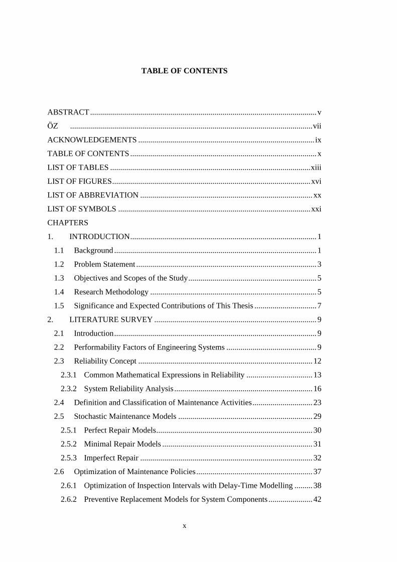
TABLE OF CONTENTS

ABSTRACT ................................................................................................................. v

ÖZ ......................................................................................................................... vii

ACKNOWLEDGEMENTS ........................................................................................ ix

TABLE OF CONTENTS ............................................................................................. x

LIST OF TABLES .................................................................................................... xiii

LIST OF FIGURES ................................................................................................... xvi

LIST OF ABBREVIATION ...................................................................................... xx

LIST OF SYMBOLS ................................................................................................ xxi

CHAPTERS

1. INTRODUCTION ............................................................................................. 1

1.1 Background ..................................................................................................... 1

1.2 Problem Statement .......................................................................................... 3

1.3 Objectives and Scopes of the Study ................................................................ 5

1.4 Research Methodology ................................................................................... 5

1.5 Significance and Expected Contributions of This Thesis ............................... 7

2. LITERATURE SURVEY ................................................................................. 9

2.1 Introduction ..................................................................................................... 9

2.2 Performability Factors of Engineering Systems ............................................. 9

2.3 Reliability Concept ....................................................................................... 12

2.3.1 Common Mathematical Expressions in Reliability ................................. 13

2.3.2 System Reliability Analysis ..................................................................... 16

2.4 Definition and Classification of Maintenance Activities .............................. 23

2.5 Stochastic Maintenance Models ................................................................... 29

2.5.1 Perfect Repair Models .............................................................................. 30

2.5.2 Minimal Repair Models ........................................................................... 31

2.5.3 Imperfect Repair ...................................................................................... 32

2.6 Optimization of Maintenance Policies .......................................................... 37

2.6.1 Optimization of Inspection Intervals with Delay-Time Modelling ......... 38

2.6.2 Preventive Replacement Models for System Components ...................... 42

xi

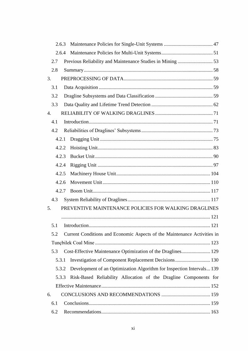
2.6.3 Maintenance Policies for Single-Unit Systems ....................................... 47

2.6.4 Maintenance Policies for Multi-Unit Systems ......................................... 51

2.7 Previous Reliability and Maintenance Studies in Mining ............................ 53

2.8 Summary ....................................................................................................... 58

3. PREPROCESSING OF DATA ....................................................................... 59

3.1 Data Acquisition ........................................................................................... 59

3.2 Dragline Subsystems and Data Classification .............................................. 59

3.3 Data Quality and Lifetime Trend Detection ................................................. 62

4. RELIABILITY OF WALKING DRAGLINES .............................................. 71

4.1 Introduction ................................................................................................... 71

4.2 Reliabilities of Draglines’ Subsystems ......................................................... 73

4.2.1 Dragging Unit .......................................................................................... 75

4.2.2 Hoisting Unit............................................................................................ 83

4.2.3 Bucket Unit .............................................................................................. 90

4.2.4 Rigging Unit ............................................................................................ 97

4.2.5 Machinery House Unit ........................................................................... 104

4.2.6 Movement Unit ...................................................................................... 110

4.2.7 Boom Unit.............................................................................................. 117

4.3 System Reliability of Draglines .................................................................. 117

5. PREVENTIVE MAINTENANCE POLICIES FOR WALKING DRAGLINES

....................................................................................................................... 121

5.1 Introduction ................................................................................................. 121

5.2 Current Conditions and Economic Aspects of the Maintenance Activities in

Tunçbilek Coal Mine ............................................................................................ 123

5.3 Cost-Effective Maintenance Optimization of the Draglines....................... 129

5.3.1 Investigation of Component Replacement Decisions ............................ 130

5.3.2 Development of an Optimization Algorithm for Inspection Intervals ... 139

5.3.3 Risk-Based Reliability Allocation of the Dragline Components for

Effective Maintenance ....................................................................................... 152

6. CONCLUSIONS AND RECOMMENDATIONS ....................................... 159

6.1 Conclusions ................................................................................................. 159

6.2 Recommendations ....................................................................................... 163

xii

REFERENCES ......................................................................................................... 165

APPENDICES

A. PREVENTIVE REPLACEMENT INTERVAL CURVES ................................ 177

B. AGE-REPLACEMENT INTERVALS OF DRAGLINE COMPONENTS ........ 183

CIRRICULUM VITAE ............................................................................................ 185

xiii

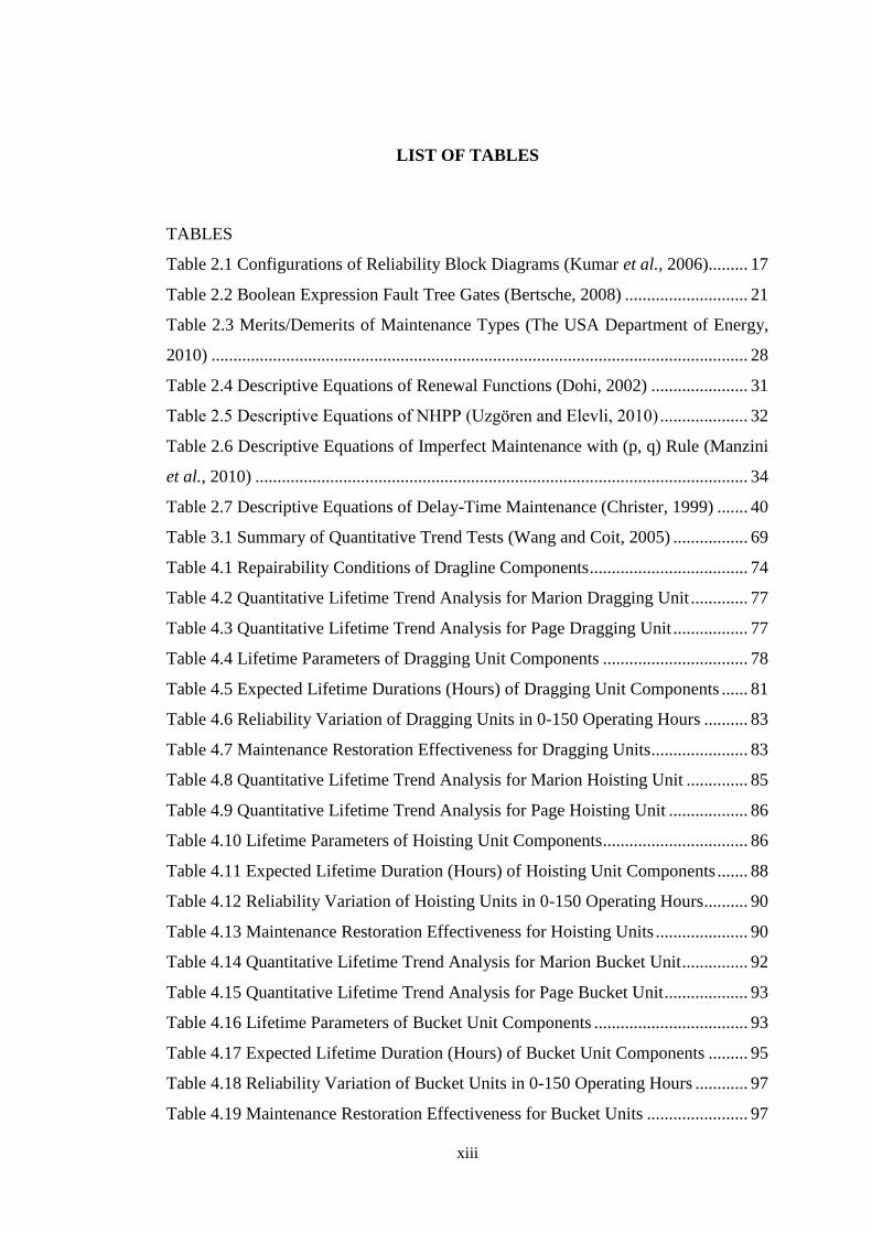
LIST OF TABLES

TABLES

Table 2.1 Configurations of Reliability Block Diagrams (Kumar et al., 2006)......... 17

Table 2.2 Boolean Expression Fault Tree Gates (Bertsche, 2008) ............................ 21

Table 2.3 Merits/Demerits of Maintenance Types (The USA Department of Energy,

2010) .......................................................................................................................... 28

Table 2.4 Descriptive Equations of Renewal Functions (Dohi, 2002) ...................... 31

Table 2.5 Descriptive Equations of NHPP (Uzgören and Elevli, 2010) .................... 32

Table 2.6 Descriptive Equations of Imperfect Maintenance with (p, q) Rule (Manzini

et al., 2010) ................................................................................................................ 34

Table 2.7 Descriptive Equations of Delay-Time Maintenance (Christer, 1999) ....... 40

Table 3.1 Summary of Quantitative Trend Tests (Wang and Coit, 2005) ................. 69

Table 4.1 Repairability Conditions of Dragline Components .................................... 74

Table 4.2 Quantitative Lifetime Trend Analysis for Marion Dragging Unit ............. 77

Table 4.3 Quantitative Lifetime Trend Analysis for Page Dragging Unit ................. 77

Table 4.4 Lifetime Parameters of Dragging Unit Components ................................. 78

Table 4.5 Expected Lifetime Durations (Hours) of Dragging Unit Components ...... 81

Table 4.6 Reliability Variation of Dragging Units in 0-150 Operating Hours .......... 83

Table 4.7 Maintenance Restoration Effectiveness for Dragging Units...................... 83

Table 4.8 Quantitative Lifetime Trend Analysis for Marion Hoisting Unit .............. 85

Table 4.9 Quantitative Lifetime Trend Analysis for Page Hoisting Unit .................. 86

Table 4.10 Lifetime Parameters of Hoisting Unit Components ................................. 86

Table 4.11 Expected Lifetime Duration (Hours) of Hoisting Unit Components ....... 88

Table 4.12 Reliability Variation of Hoisting Units in 0-150 Operating Hours .......... 90

Table 4.13 Maintenance Restoration Effectiveness for Hoisting Units ..................... 90

Table 4.14 Quantitative Lifetime Trend Analysis for Marion Bucket Unit ............... 92

Table 4.15 Quantitative Lifetime Trend Analysis for Page Bucket Unit ................... 93

Table 4.16 Lifetime Parameters of Bucket Unit Components ................................... 93

Table 4.17 Expected Lifetime Duration (Hours) of Bucket Unit Components ......... 95

Table 4.18 Reliability Variation of Bucket Units in 0-150 Operating Hours ............ 97

Table 4.19 Maintenance Restoration Effectiveness for Bucket Units ....................... 97

xiv

Table 4.20 Quantitative Lifetime Trend Analysis for Marion Rigging Unit ............. 99

Table 4.21 Quantitative Lifetime Trend Analysis for Page Rigging Unit ................. 99

Table 4.22 Lifetime Parameters of Rigging Unit Components ................................ 100

Table 4.23 Expected Lifetime Duration (Hours) of Rigging Unit Components ...... 102

Table 4.24 Reliability Variation of Rigging Units in 0-150 Operating Hours ......... 103

Table 4.25 Maintenance Restoration Effectiveness for Rigging Units .................... 104

Table 4.26 Quantitative Lifetime Trend Analysis for Marion MH Unit .................. 106

Table 4.27 Quantitative Lifetime Trend Analysis for Page MH Unit ...................... 106

Table 4.28 Lifetime Parameters of MH Unit Components ...................................... 107

Table 4.29 Expected Lifetime Duration (Hours) of MH Unit Components ............ 108

Table 4.30 Reliability Variation of MH Unit in 0-150 Operating Hours ................. 110

Table 4.31 Maintenance Restoration Effectiveness for MH Units .......................... 110

Table 4.32 Quantitative Lifetime Trend Analysis for Marion Movement Unit ....... 112

Table 4.33 Quantitative Lifetime Trend Analysis for Page Movement Unit ........... 113

Table 4.34 Lifetime Parameters of Movement Unit Components ........................... 113

Table 4.35 Expected Lifetime Duration (Hours) of Movement Unit Components . 115

Table 4.36 Reliability Variation of Movement Units in 0-150 Operating Hours .... 116

Table 4.37 Maintenance Restoration Effectiveness for Movement Units ............... 117

Table 4.38 Boom Unit Lifetime Parameters using General Renewal Function ....... 117

Table 4.39 Time-Dependent Reliability and Mean Lifetimes of Draglines ............. 119

Table 5.1 Unit Production Losses ($) of the Draglines ............................................ 124

Table 5.2 Repair Time Distributions and MTTR Values of Dragline Components 125

Table 5.3 Direct and Expected Indirect Costs of Dragline Component Failures ..... 126

Table 5.4 Annual Downtime Profiles of the Draglines ............................................ 127

Table 5.5 Costs of Corrective and Preventive Component Replacements ............... 132

Table 5.6 Age-Replacement Policy Equations ......................................................... 133

Table 5.7 Age-Replacement Intervals for the Wear-Out Components .................... 136

Table 5.8 Preventive Inspection Costs and FTD Values of Dragline Components . 147

Table 5.9 Variation of Total Maintenance Costs According to Inspection Intervals

.................................................................................................................................. 148

Table 5.10 RPN Occurrence Factor (The USA Department of Army, 2006) .......... 153

Table 5.11 Risk Priority Numbers of Dragline Components ................................... 154

xv

Table 5.12 Reliability Allocation of Page Components for Target Reliabilities ..... 157

Table 5.13 Reliability Allocation of Marion Components for Target Reliabilities . 158

Table B.1 Age-Replacement Intervals of Marion Wear-out Components ............... 183

Table B.2 Age-Replacement Intervals of Page Wear-out Components ................... 184

xvi

LIST OF FIGURES

FIGURES

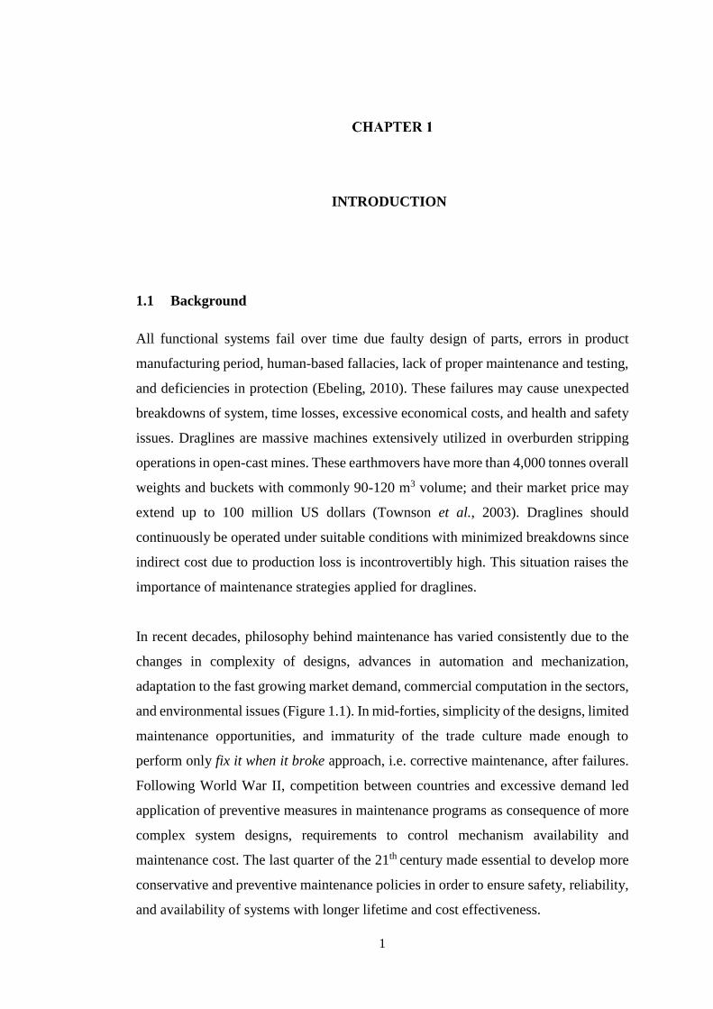
Figure 1.1 Development of Maintenance Philosophy (Moubray, 1997) ...................... 2

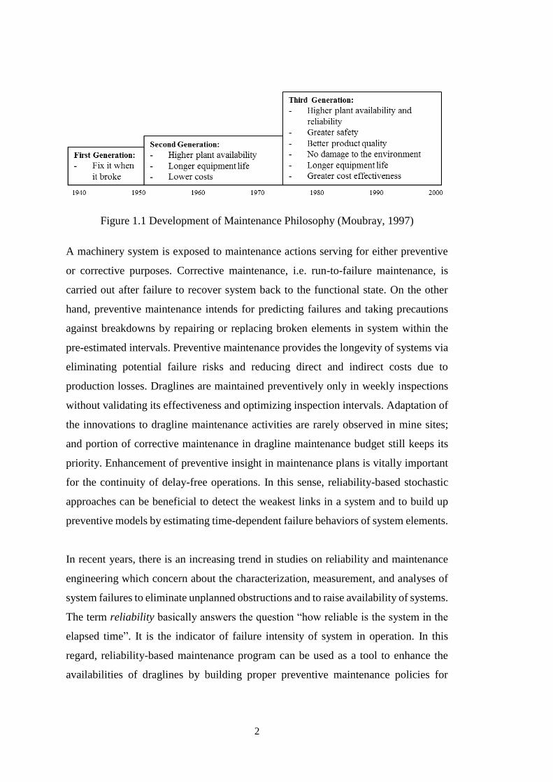
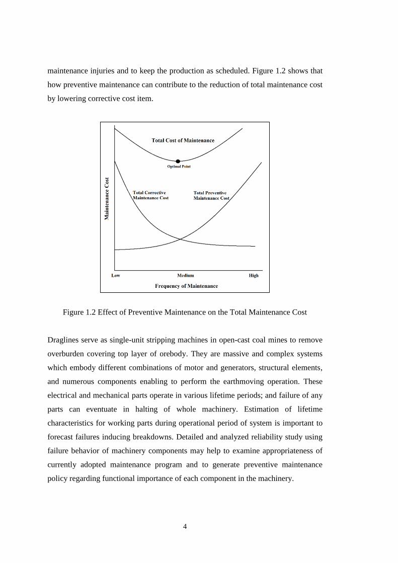
Figure 1.2 Effect of Preventive Maintenance on the Total Maintenance Cost ............ 4

Figure 1.3 Research Methodology of the Thesis Study ............................................... 7

Figure 2.1 Performability Factors of Engineering Systems (Misra, 2008) ................ 10

Figure 2.2 Operational Downtimes of Systems (Modified after Dhillon, 1999) ....... 12

Figure 2.3 Mean Time Parameters (Modified after Bertsche, 2008) ......................... 15

Figure 2.4 FTA Gate and Event Symbols (Reliasoft R&D Staff, 2004) .................... 21

Figure 2.5 Transitions in Markov Chains (Smith, 2001) ........................................... 22

Figure 2.6 Types of Maintenance (Mishra and Pathak, 2004) ................................... 24

Figure 2.7 Percentage Distributions of Maintenance Activities (The USA Department

of Energy, 2010) ......................................................................................................... 25

Figure 2.8 Utilization Areas of Reliability-Based Maintenance (Dhillon, 1999) ...... 27

Figure 2.9 Maintenance Models according to the Repairing Assumption ................. 29

Figure 2.10 Imperfect Maintenance Using (p,q) Rule (Manzini et al., 2010) ........... 33

Figure 2.11 Effect of Repair Types on Failure Rate (Blischke and Murthy, 2000) ... 35

Figure 2.12 Maintenance-Based Failure Rate Variations (Lie and Chun, 1986) ....... 35

Figure 2.13 Delay Times of Single Component ......................................................... 39

Figure 2.14 Delay Times of Multi-Component Systems ........................................... 41

Figure 2.15 Subjective Delay Times for Breakdown (a) and Inspection (b) ............. 41

Figure 3.1 A Dragline Operation and Schematic View of Dragline’s Subsystems ... 60

Figure 3.2 Failure Number and Breakdown Duration Distribution for the Draglines 61

Figure 3.3 Box Plots in Outlier Detection .................................................................. 63

Figure 3.4 Outlier Detection in Page Drag Unit Using Box Plots ............................. 63

Figure 3.5 Potential Causes of Data Randomness...................................................... 65

Figure 3.6 Run Chart for Drag Rope Component of Page Dragline .......................... 65

Figure 3.7 Sample Plot of CFN versus (a) CTBF and (b) Duane Plot ....................... 66

Figure 4.1 Methodology of the System Reliability Analysis ..................................... 72

Figure 4.2 Graphical Lifetime Trend Test for Marion Dragging Unit ....................... 76

Figure 4.3 Graphical Lifetime Trend Test for Page Dragging Unit ........................... 76

xvii

Figure 4.4 Probability Density Functions of Marion Dragging Unit Components .... 80

Figure 4.5 Probability Density Functions of Page Dragging Unit Components ........ 81

Figure 4.6 System and Component Reliability Curves of Marion Dragging Unit .... 82

Figure 4.7 System and Component Reliability Curves of Page Dragging Unit ........ 82

Figure 4.8 Graphical Lifetime Trend Test for Marion Hoisting Unit ........................ 84

Figure 4.9 Graphical Lifetime Trend Test for Page Hoisting Unit ............................ 85

Figure 4.10 Probability Density Functions of Marion Hoisting Unit Components ... 87

Figure 4.11 Probability Density Functions of Page Hoisting Unit Component ......... 88

Figure 4.12 System and Component Reliability Curves of Marion Hoisting Unit .... 89

Figure 4.13 System and Component Reliability Curves of Page Hoisting Unit ........ 89

Figure 4.14 Graphical Lifetime Trend Test for Marion Bucket Unit ........................ 91

Figure 4.15 Graphical Lifetime Trend Test for Page Bucket Unit ............................ 92

Figure 4.16 Probability Density Functions of Marion Bucket Unit Components ..... 94

Figure 4.17 Probability Density Functions of Page Bucket Unit Components ......... 95

Figure 4.18 System and Component Reliability Curves of Marion Bucket Unit ...... 96

Figure 4.19 System and Component Reliability Curves of Page Bucket Unit .......... 96

Figure 4.20 Graphical Lifetime Trend Test for Marion Rigging Unit ....................... 98

Figure 4.21 Graphical Lifetime Trend Test for Page Rigging Unit ........................... 98

Figure 4.22 Probability Density Functions of Marion Rigging Unit Components .. 101

Figure 4.23 Probability Density Functions of Page Rigging Unit Components ...... 101

Figure 4.24 System and Component Reliability Curves of Marion Rigging Unit ... 102

Figure 4.25 System and Component Reliability Curves of Page Rigging Unit ....... 103

Figure 4.26 Graphical Lifetime Trend Test for Marion MH Unit ........................... 105

Figure 4.27 Graphical Lifetime Trend Test for Page MH Unit ............................... 105

Figure 4.28 Probability Density Functions of Marion MH Components ................ 107

Figure 4.29 Probability Density Functions of Page MH Components .................... 108

Figure 4.30 System and Component Reliability Curves of Marion MH Unit ......... 109

Figure 4.31 System and Component Reliability Curves of Page MH Unit ............. 109

Figure 4.32 Graphical Lifetime Trend Test for Marion Movement Unit ................ 111

Figure 4.33 Graphical Lifetime Trend Test for Page Movement Unit .................... 112

Figure 4.34 Probability Density Functions of Marion Movement Components ...... 114

Figure 4.35 Probability Density Functions of Page Movement Components .......... 114

xviii

Figure 4.36 System and Component Reliability Curves of Marion Movement Unit

.................................................................................................................................. 115

Figure 4.37 System and Component Reliability Curves of Page Movement Unit .. 116

Figure 4.38 System Reliability of Marion Dragline ................................................. 118

Figure 4.39 System Reliability of Page Dragline ..................................................... 119

Figure 5.1 Methodology of the Maintenance Optimization ..................................... 122

Figure 5.2 Sample Simulation Window for Marion System .................................... 128

Figure 5.3 Sample Simulation Window for Page System ........................................ 128

Figure 5.4 Sample Curve of Positive Replacement Decision .................................. 134

Figure 5.5 Preventive Replacement Interval Curve for Marion Dragging Socket ... 134

Figure 5.6 Preventive Replacement Interval Curve for Page Rigging Rope-Mode01

.................................................................................................................................. 135

Figure 5.7 Optimum Replacement Intervals of Marion Wear-out Components for

Different Ratios of Corrective (Cc) and Preventive (Cp) Replacement Costs .......... 137

Figure 5.8 Optimum Replacement Intervals of Page Wear-out Components for

Different Ratios of Corrective (Cc) and Preventive (Cp) Replacement Costs .......... 138

Figure 5.9 Maintenance Behavior of a Two-Components System according to the

Algorithm ................................................................................................................. 142

Figure 5.10 Flowchart of Inspection Algorithm with Constant Inspection Interval 144

Figure 5.11 Inspection Optimization Curves for the Draglines ............................... 148

Figure 5.12 Annual Corrective Maintenance Costs of Marion Units for Changing

Inspection Intervals .................................................................................................. 149

Figure 5.13 Annual Corrective Maintenance Costs of Page Units for Changing

Inspection Intervals .................................................................................................. 150

Figure 5.14 Annual Preventive Maintenance Costs of Marion Units for Changing

Inspection Intervals .................................................................................................. 151

Figure 5.15 Annual Preventive Maintenance Costs of Page Units for Changing

Inspection Intervals .................................................................................................. 151

Figure A.1 Age-Replacement Curve of Marion Dragging Ringbolt ........................ 177

Figure A.2 Age-Replacement Curve of Marion Dragging Rope-Mode01 ............... 177

Figure A.3 Age-Replacement Curve of Marion Hoisting Rope-Mode01 ................ 178

Figure A.4 Age-Replacement Curve of Marion Rigging Pulley-Mode01 ............... 178

xix

Figure A.5 Age-Replacement Curve of Marion Rigging Rope-Mode01 ................. 179

Figure A.6 Age-Replacement Curve of Page Dragging Ringbolt............................ 179

Figure A.7 Age-Replacement Curve of Page Dragging Rope-Mode01 .................. 180

Figure A.8 Age-Replacement Curve of Page Hoisting Brake ................................. 180

Figure A.9 Age-Replacement Curve of Page Hoisting Rope-Mode01 .................... 181

Figure A.10 Age-Replacement Curve of Page Rigging Pulley-Mode01 ................. 181

Figure A.11 Age-Replacement Curve of Page Rigging Socket ............................... 182

xx

LIST OF ABBREVIATION

ARP Alternating Renewal Process

CDF Cumulative Density Function

CFN Cumulative Failure Number

FMEA Failure Modes and Effects Analysis

FMECA Failure Modes Effects and Criticality Analysis

FTA Fault Tree Analysis

GRP General Renewal Process

HPP Homogenous Poisson Process

IQR Inter-quartile Range

MTBF Mean Time between Failures

MTTF Mean Time to Failure

MTTFF Mean Time to First Failure

MTTR Mean Time to Repair

NHPP Non-Homogenous Poisson Process

ORP Ordinary Renewal Process

PDF Failure Probability Density Function

RBD Reliability Block Diagram

RPN Risk Priority Number

TBF Time between Failures

TTR Time to Repair

xxi

LIST OF SYMBOLS

R(t), F̅(t) Reliability (Survival) Function

F(t) Failure (Unreliability) Function

f(t) Failure Probability Density Function

P(x) Probability for the Occurrence of Event x

P(x̅) Probability for the Occurrence of Complementary Event x

E(t), μ Mathematical Expectation

s, σ Standard Deviation

tmedian, T50 Median Time

tmodal Modal Time (Mode)

λ(t), r(t) Failure Rate

μ(t) Repair Rate

Bq Certain Time Period with Failure Probability of q

N(t) Number of Failures at Time t

Sn Cumulative Time between Failures

M(t) Renewal Function

EX Expected Uptime

EY Expected Downtime

G(t) Distribution Function of Downtimes

H(t) Convolution of Uptime (F(t)) and Downtime G(t) Functions

Cf Cost of Failure Maintenance

Cp Cost of Preventive Maintenance

Ci Cost of Inspection

q Probability of Perfect Repair

p Probability of Minimal Repair

xxii

1

1. INTRODUCTION

1.1 Background

All functional systems fail over time due faulty design of parts, errors in product

manufacturing period, human-based fallacies, lack of proper maintenance and testing,

and deficiencies in protection (Ebeling, 2010). These failures may cause unexpected

breakdowns of system, time losses, excessive economical costs, and health and safety

issues. Draglines are massive machines extensively utilized in overburden stripping

operations in open-cast mines. These earthmovers have more than 4,000 tonnes overall

weights and buckets with commonly 90-120 m3 volume; and their market price may

extend up to 100 million US dollars (Townson et al., 2003). Draglines should

continuously be operated under suitable conditions with minimized breakdowns since

indirect cost due to production loss is incontrovertibly high. This situation raises the

importance of maintenance strategies applied for draglines.

In recent decades, philosophy behind maintenance has varied consistently due to the

changes in complexity of designs, advances in automation and mechanization,

adaptation to the fast growing market demand, commercial computation in the sectors,

and environmental issues (Figure 1.1). In mid-forties, simplicity of the designs, limited

maintenance opportunities, and immaturity of the trade culture made enough to

perform only fix it when it broke approach, i.e. corrective maintenance, after failures.

Following World War II, competition between countries and excessive demand led

application of preventive measures in maintenance programs as consequence of more

complex system designs, requirements to control mechanism availability and

maintenance cost. The last quarter of the 21th century made essential to develop more

conservative and preventive maintenance policies in order to ensure safety, reliability,

and availability of systems with longer lifetime and cost effectiveness.

2

Figure 1.1 Development of Maintenance Philosophy (Moubray, 1997)

A machinery system is exposed to maintenance actions serving for either preventive

or corrective purposes. Corrective maintenance, i.e. run-to-failure maintenance, is

carried out after failure to recover system back to the functional state. On the other

hand, preventive maintenance intends for predicting failures and taking precautions

against breakdowns by repairing or replacing broken elements in system within the

pre-estimated intervals. Preventive maintenance provides the longevity of systems via

eliminating potential failure risks and reducing direct and indirect costs due to

production losses. Draglines are maintained preventively only in weekly inspections

without validating its effectiveness and optimizing inspection intervals. Adaptation of

the innovations to dragline maintenance activities are rarely observed in mine sites;

and portion of corrective maintenance in dragline maintenance budget still keeps its

priority. Enhancement of preventive insight in maintenance plans is vitally important

for the continuity of delay-free operations. In this sense, reliability-based stochastic

approaches can be beneficial to detect the weakest links in a system and to build up

preventive models by estimating time-dependent failure behaviors of system elements.

In recent years, there is an increasing trend in studies on reliability and maintenance

engineering which concern about the characterization, measurement, and analyses of

system failures to eliminate unplanned obstructions and to raise availability of systems.

The term reliability basically answers the question “how reliable is the system in the

elapsed time”. It is the indicator of failure intensity of system in operation. In this

regard, reliability-based maintenance program can be used as a tool to enhance the

availabilities of draglines by building proper preventive maintenance policies for

3

critical components in the system. In addition, deductive algorithm of reliability

methods may assist to realize root-causes of dragline breakdowns.

1.2 Problem Statement

The design of a qualified system motives engineers to manufacture product with high

reliability, longevity, and minimal maintenance cost in addition to satisfying its

functional requirements. Increase in the complexity of a system boosts the severity of

the time-dependent availability since many components may lead to breakdown of

system in short to long-term. In mining industry, demanding working conditions and

high rate of machine utilization generally cause frequent failures of machinery

components and compulsory pause of production in the sequel. Commercial pressure

on mining sector for continual production forces maintenance staff to recover the failed

machine back to functional state in short periods. Frequency of corrective maintenance

increases operating cost and also negatively affects production scheduling. Researches

showed that 40 to 50% of the equipment operating cost is spent on only maintenance

expenses (Forsmann and Kumar, 1992) which is approximately equal to 20-35% of

the total operating cost in a mine (Unger and Conway, 1994). In addition to direct cost

of maintenance, length of downtime induces indirect costs due to production losses,

delays in scheduling, and even deterioration of company image in industry. For

Australian coal mines, it was realized that production loss based on unplanned

maintenance may reach to 10% (Clark, 1990). Moreover, there is another hidden cost

due to the aging and early death of machines due to improper maintenance works.

Rapid progressive of aging problem leads to replacement of machines prior to their

expected mean lifetimes. In addition to the cost factors, high frequency of the failures

and unorganized structure of maintenance may lead to rise in occupational injuries.

The USA Mine Safety and Health Administration (MSHA) data between 2001 and

2003 pointed out that 15% of the recorded mining injuries in the United States appears

to happen during maintenance activities (Smith et al., 2004). Most of the negative

issues mentioned above are generally due to unplanned work-flow of maintenance

programs and fix it when it broke approach in maintenance policies. In this sense,

planned preventive maintenance policy can assist to reduce unexpected cost and

4

maintenance injuries and to keep the production as scheduled. Figure 1.2 shows that

how preventive maintenance can contribute to the reduction of total maintenance cost

by lowering corrective cost item.

Figure 1.2 Effect of Preventive Maintenance on the Total Maintenance Cost

Draglines serve as single-unit stripping machines in open-cast coal mines to remove

overburden covering top layer of orebody. They are massive and complex systems

which embody different combinations of motor and generators, structural elements,

and numerous components enabling to perform the earthmoving operation. These

electrical and mechanical parts operate in various lifetime periods; and failure of any

parts can eventuate in halting of whole machinery. Estimation of lifetime

characteristics for working parts during operational period of system is important to

forecast failures inducing breakdowns. Detailed and analyzed reliability study using

failure behavior of machinery components may help to examine appropriateness of

currently adopted maintenance program and to generate preventive maintenance

policy regarding functional importance of each component in the machinery.

5

1.3 Objectives and Scopes of the Study

The main objective of research study is to develop reliability-based maintenance

optimization model for Page and Marion draglines utilized in Tunçbilek Coal Mine.

Constituents of this objective cover: (i) development of a system reliability model

which identifies all structural dependencies between sub-units and components, (ii)

simulation of currently utilized maintenance policy for the draglines considering cost

and availability measures, (iv) optimization of the maintenance policy using stochastic

replacement and inspection models, (v) detection of maintenance-critical components

using risk-based reliability allocation models, and (vi) demonstration of cost-

effectiveness for the optimized maintenance policy.

The scope of this study covers only two draglines currently operating in Tunçbilek

coal mine and the maintenance data utilized for the study is for 1998-2011 period.

Details of maintenance activities and cost values used in the thesis were specified

considering opinions of dragline maintenance experts in Tunçbilek coal mine. The cost

values are up-to-date values of year 2015.

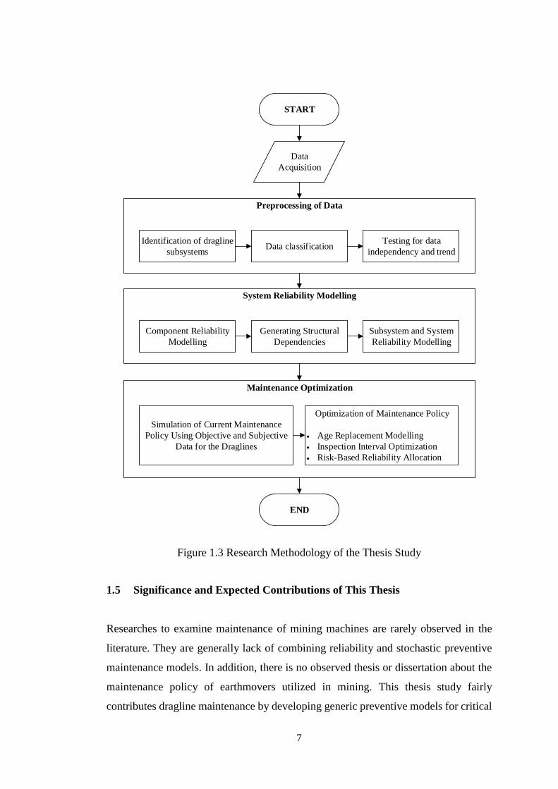
1.4 Research Methodology

This research study utilizes statistical and probabilistic approaches to investigate the

time-dependent reliability of draglines and to develop an optimization platform for

maintenance of these earthmovers. Graphical illustration of the research methodology

is given in Figure 1.3. Main stages of the research methodology is as follows:

i. Preprocessing of data: (a) Data in between 1998 and 2011 was acquired. It covers

the breakdown information of two draglines, Page 736 and Marion 7820, which are

still utilized in Tunçbilek coal mine owned by Turkish Coal Enterprises. (b)

Dragline was divided into seven subsystems regarding their functional states in

system; and individual components were distributed to subsystems. (c) Time

between failures and time to repair data were assigned to individual components.

(d) Grouped data was statistically tested to detect possible trend, independency,

autocorrelation, and outlier occurrences.

6

ii. System Reliability Analysis: (a) Reliability of individual components were

evaluated using general renewal process or best-fit distributions according to data

trend behavior. Lifetime characteristics of components were identified using

Reliasoft Weibull++7 software. Parameters of each model were analyzed to

comprehend failure behaviors and expected lifetimes of components. (b) Structural

dependency in the system was identified using Reliasoft Blocksim++7 to build up

system reliability model. (c) Failure rate, reliability, availability, and reliability

importance were utilized to designate failure intensities (functional criticality) of

components in the system.

iii. Maintenance Policy Modelling: (a) Current maintenance policy of draglines applied

in the mine was simulated in Reliasoft Blocksim++7 to evaluate expected

downtimes of draglines due to failures and compulsory breaks in shifts and

inspections. (b) In optimization stage, age-replacement policies were developed to

examine the feasibility of preventive replacement for the components in wear-out

period. (c) An algorithm was generated to find out the optimal inspection intervals

for draglines. This algorithm considered the scheduled halts during shifts and

inspections, random lifetime and repair behaviors of system components, and their

effects on system in case of failures. It aimed to minimize overall maintenance cost

via investigating effect of inspection intervals on the cost. (d) A risk-based

reliability allocation model was developed to reveal the most critical components.

iv. Result Interpretation: (a) Cost effectiveness of the improved model was interpreted

compare to the previous policy (b) Sensitivity of corrective and preventive

maintenance costs to a maintenance policy were evaluated. (c) Contributions of

optimization study to the current maintenance policy were assessed.

7

START

Data

Acquisition

Preprocessing of Data

Identification of dragline

subsystemsData classification

Testing for data

independency and trend

System Reliability Modelling

Component Reliability

Modelling

Generating Structural

Dependencies

Subsystem and System

Reliability Modelling

Maintenance Optimization

Simulation of Current Maintenance

Policy Using Objective and Subjective

Data for the Draglines

Optimization of Maintenance Policy

Age Replacement Modelling

Inspection Interval Optimization

Risk-Based Reliability Allocation

END

Figure 1.3 Research Methodology of the Thesis Study

1.5 Significance and Expected Contributions of This Thesis

Researches to examine maintenance of mining machines are rarely observed in the

literature. They are generally lack of combining reliability and stochastic preventive

maintenance models. In addition, there is no observed thesis or dissertation about the

maintenance policy of earthmovers utilized in mining. This thesis study fairly

contributes dragline maintenance by developing generic preventive models for critical

8

components using retroactive failure data. The dissertation implement a generic cost-

effective inspection optimization algorithm, considering corrective and preventive

maintenance costs, random component lifetimes, and random repair durations.

Therefore, the research gives opportunity to investigate the contributions of corrective

and preventive maintenance on total maintenance cost for changing inspection

intervals. The developed methodologies in the thesis can be applied for reliability

assessment and maintenance optimization of any machinery system. Therefore,

decision makers in machinery maintenance can apply these methodologies to their own

systems in order to investigate feasibility of their current maintenance strategy or to

develop new cost- and availability- effective maintenance policies.

9

2. LITERATURE SURVEY

2.1 Introduction

An extensive literature survey was carried out to comprehend the underlying theories

and methodologies regarding reliability and maintenance of systems. The literature

survey covers the issues on system effectiveness factors, reliability and maintenance

concepts, system reliability models, stochastic modelling of maintenance policies, and

recent studies on maintenance and reliability of mining systems.

2.2 Performability Factors of Engineering Systems

The origin of the word system comes from Greek word of systema which denotes

leaguing together and it basically signifies the union of interoperable components

holding individual restricted capacities and operating together to manage a mutual

mission in a prescribed working condition with a desired success (Wasson, 2006).

Performance of a system may be influenced by various factors originated from

manufacturing process, utilization conditions and environment considerations. In this

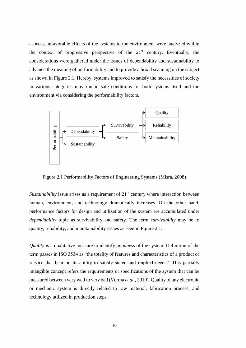
sense, Misra (2008) discussed the effectiveness factors under the terms of

performability, dependability, sustainability, survivability, safety, reliability,

maintainability, and quality as illustrated in Figure 2.1. These terms are called as 3S-

parameters (Survivability-Safety-Sustainability).

Performability was firstly introduced by Meyer (1980) to interpret the effectiveness of

monitoring systems for NASA aircrafts. In early times, performability only covered

the topics of reliability, maintainability, and availability. Later on, accessional

requirement on the definition of system effectiveness forced engineers to think about

different attributes of system performance. In addition to the economy and safety

10

aspects, unfavorable effects of the systems to the environment were analyzed within

the context of progressive perspective of the 21st century. Eventually, the

considerations were gathered under the issues of dependability and sustainability to

advance the meaning of performability and to provide a broad scanning on the subject

as shown in Figure 2.1. Hereby, systems improved to satisfy the necessities of society

in various categories may run in safe conditions for both systems itself and the

environment via considering the performability factors.

Figure 2.1 Performability Factors of Engineering Systems (Misra, 2008)

Sustainability issue arises as a requirement of 21th century where interaction between

human, environment, and technology dramatically increases. On the other hand,

performance factors for design and utilization of the system are accumulated under

dependability topic as survivability and safety. The term survivability may be to

quality, reliability, and maintainability issues as seen in Figure 2.1.

Quality is a qualitative measure to identify goodness of the system. Definition of the

term passes in ISO 3534 as “the totality of features and characteristics of a product or

service that bear on its ability to satisfy stated and implied needs”. This partially

intangible concept refers the requirements or specifications of the system that can be

measured between very well to very bad (Verma et al., 2010). Quality of any electronic

or mechanic system is directly related to raw material, fabrication process, and

technology utilized in production steps.

Per

form

abil

ity

Dependability

Survivability

Quality

Reliability

MaintainabilitySafety

Sustainability

11

In addition to quality, reliability issue includes qualitative and/or quantitative analysis

of a system to measure the success to keep system functionality without failure in a

specified time interval and environment using interdisciplinary approaches of

engineering, probability, and statistics. Reliability holds four main parameters as

probability, adequate performance, time, and operating and environment conditions

(Aggarwal, 1993). Reliability analyses reveal substantive results about operating

performance of systems if boundaries of systems to be analyzed are determined

precisely. A reliability analysis gives opportunity for (i) investigation of the functional

continuity in working systems, (ii) forecasting possible interruptions and their

consequences, and (iii) developing a conservative and optimal maintenance policy.

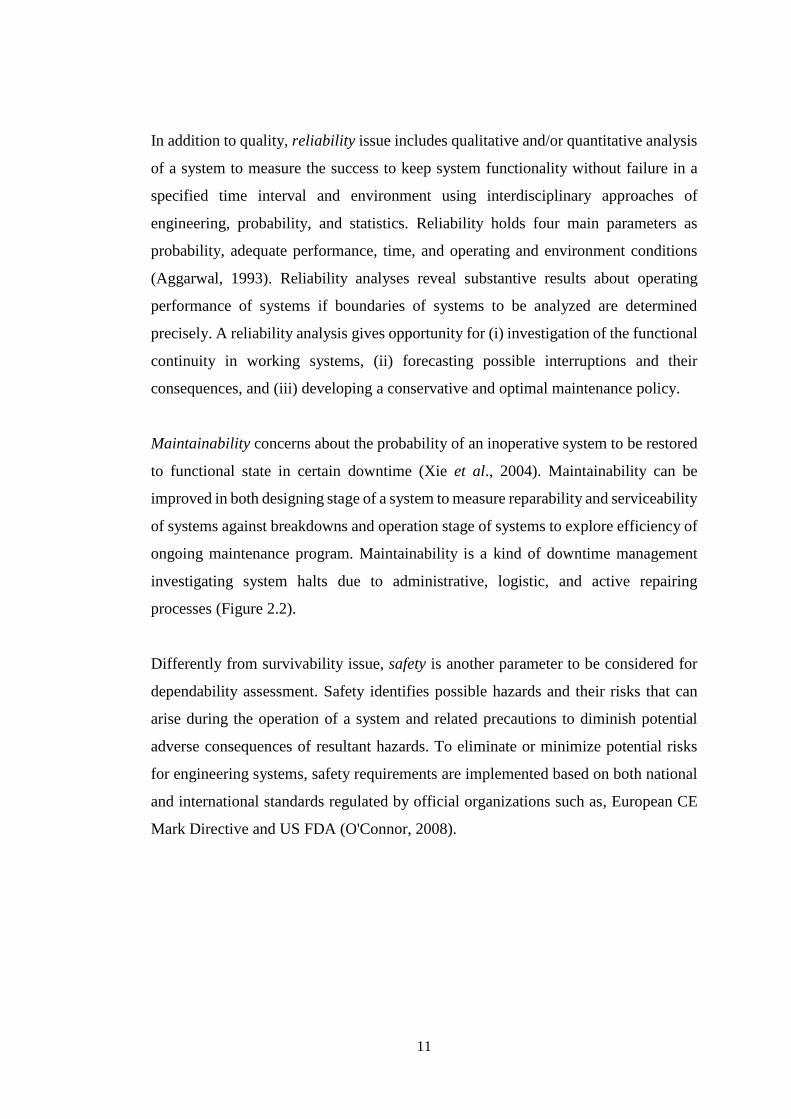
Maintainability concerns about the probability of an inoperative system to be restored

to functional state in certain downtime (Xie et al., 2004). Maintainability can be

improved in both designing stage of a system to measure reparability and serviceability

of systems against breakdowns and operation stage of systems to explore efficiency of

ongoing maintenance program. Maintainability is a kind of downtime management

investigating system halts due to administrative, logistic, and active repairing

processes (Figure 2.2).

Differently from survivability issue, safety is another parameter to be considered for

dependability assessment. Safety identifies possible hazards and their risks that can

arise during the operation of a system and related precautions to diminish potential

adverse consequences of resultant hazards. To eliminate or minimize potential risks

for engineering systems, safety requirements are implemented based on both national

and international standards regulated by official organizations such as, European CE

Mark Directive and US FDA (O'Connor, 2008).

12

Logistic Delay Total Product Downtime Administrative Delay

Active Repair Time

Fault Location

Time

Failure

Verification TimeRepair Time

Part Acquisition

TimePreparation TimeFinal Test Time

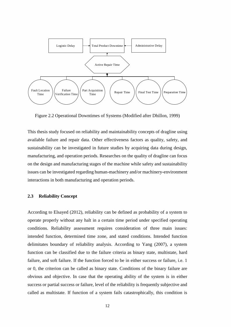
Figure 2.2 Operational Downtimes of Systems (Modified after Dhillon, 1999)

This thesis study focused on reliability and maintainability concepts of dragline using

available failure and repair data. Other effectiveness factors as quality, safety, and

sustainability can be investigated in future studies by acquiring data during design,

manufacturing, and operation periods. Researches on the quality of dragline can focus

on the design and manufacturing stages of the machine while safety and sustainability

issues can be investigated regarding human-machinery and/or machinery-environment

interactions in both manufacturing and operation periods.

2.3 Reliability Concept

According to Elsayed (2012), reliability can be defined as probability of a system to

operate properly without any halt in a certain time period under specified operating

conditions. Reliability assessment requires consideration of three main issues:

intended function, determined time zone, and stated conditions. Intended function

delimitates boundary of reliability analysis. According to Yang (2007), a system

function can be classified due to the failure criteria as binary state, multistate, hard

failure, and soft failure. If the function forced to be in either success or failure, i.e. 1

or 0, the criterion can be called as binary state. Conditions of the binary failure are

obvious and objective. In case that the operating ability of the system is in either

success or partial success or failure, level of the reliability is frequently subjective and

called as multistate. If function of a system fails catastrophically, this condition is

13

called as hard failures. Lastly, soft failure is the partial loss of operating ability that

results in multistate products. In addition to intended function type, period of time is

the main consideration to quantify the reliability since the reliability is a function of

time. Time period to be assessed can be about warranty time, scheduled operation time

or another intended period of time. Besides the time factor, operation condition is also

critical to evaluate system model realistically. The reliability conditions can describe

with system behaviors covering mechanical, electrical, thermal or another level of

product property.

2.3.1 Common Mathematical Expressions in Reliability

Reliability concept utilizes probabilistic approaches to quantify the operational

stability of systems. Probabilistic definition of reliability function, i.e. survival

function R(t), and unreliability function, i.e. failure function F(t), can be expressed

mathematically as in Equations 2.1-2.6. Failure probability density function (PDF), i.e.

f(t), is basically time-dependent probability of a system to fail (Equation 2.1). It is

actually a frequency curve of failure occurrences. In an infinite period of time, PDF is

equal to 1 since it ensures a certain failure condition as shown in Equation 2.2

(Lazzorini et al., 2011).

𝑓(𝑡) =𝑑𝐹(𝑡)

𝑑𝑡= −

𝑑𝑅(𝑡)

𝑑𝑡 (2.1)

∫ 𝑓(𝑡)𝑑𝑡 = 1∞

0 (2.2)

For time t, probability of the system not to fail in a random failure time tf is stated in

Equation 2.3 (Lazzorini et al., 2011). This situation refers survival probability of

system, i.e. reliability, at time t. It can be also expressed as the area under the failure

probability density function at right-hand side of the time, t, as in Equation 2.4

(Lazzorini et al., 2011).

𝑅(𝑡) = 𝑃{𝑡𝑓 > 𝑡} (2.3)

14

𝑅(𝑡) = �̅�(𝑡) = ∫ 𝑓(𝑡)𝑑𝑡∞

𝑡 (2.4)

Since sum of probabilities to survive and to fail is equal to 1, failure function can be

defined as in the Equation 2.5 (Lazzorini et al., 2011). It is also the area under the

failure probability function between time 0 and time t as given in Equation 2.6

(Lazzorini et al., 2011). Exponential, Weibull and lognormal distributions are

commonly utilized distribution to identify f(t).

𝐹(𝑡) = 1 − 𝑅(𝑡) = 𝑃{𝑡𝑓 < 𝑡} (2.5)

𝐹(𝑡) = ∫ 𝑓(𝑡)𝑑𝑡𝑡

0 (2.6)

In the reliability studies, some statistical measures are extensively utilized to

characterize failure behaviors. Statistical values help to realize central tendency of the

distribution and spread of the data in the density function. The most frequently utilized

statistical measures are mean, empirical variance, empirical standard deviation,

median, and mode. In addition to general statistical terms, mean time to failure

(MTTF), mean time to first failure (MTTFF), mean time between failures (MTBF),

failure rate (𝜆), and 𝐵𝑞 lifetime are commonly utilized in reliability.

As Levin and Kalal (2003) mentioned, MTTF is used to define the reliability of non-

repairable systems. On the other hand, MTBF is a term used to describe the reliability

of reparable systems and refers the average time period between the failures. However,

it should be noticed that a repairable system can consist of non-repairable sub-

components. Therefore, lifetime of a repairable system may also be evaluated in terms

of MTTF values of non-repairable system elements. MTTF is expressed

mathematically as in Equation 2.7 (Ebeling, 2010). It is sometimes notated as 𝐸(𝑡)

which means mathematical expectation.

𝑀𝑇𝑇𝐹 = 𝐸(𝑇) = ∫ 𝑡 𝑓(𝑡)𝑑𝑡 = ∫ 𝑅(𝑡)𝑑𝑡∞

0

∞

0 (2.7)

15

According to the reliability and maintainability standards such as, DEF-STAN-00-40

and MIL-HDBK-217, MTBF can be defined as in Equation 2.8 (Kumar et al., 2006).

In Equation 2.8, T refers the total operating time and n is the number of failure during

the period covering the stated operating time. MTBF is equal to MTTF if the

maintenance after failure recovers the system to as good as new condition.

𝑀𝑇𝐵𝐹 = 𝑇/𝑛 (2.8)

On the other hand, MTTFF estimates mean time to the first failure. For new reparable

systems, it can take a long time to face with first failure. Therefore, it is beneficial to

consider failure behavior after the first failure when establishing a maintenance

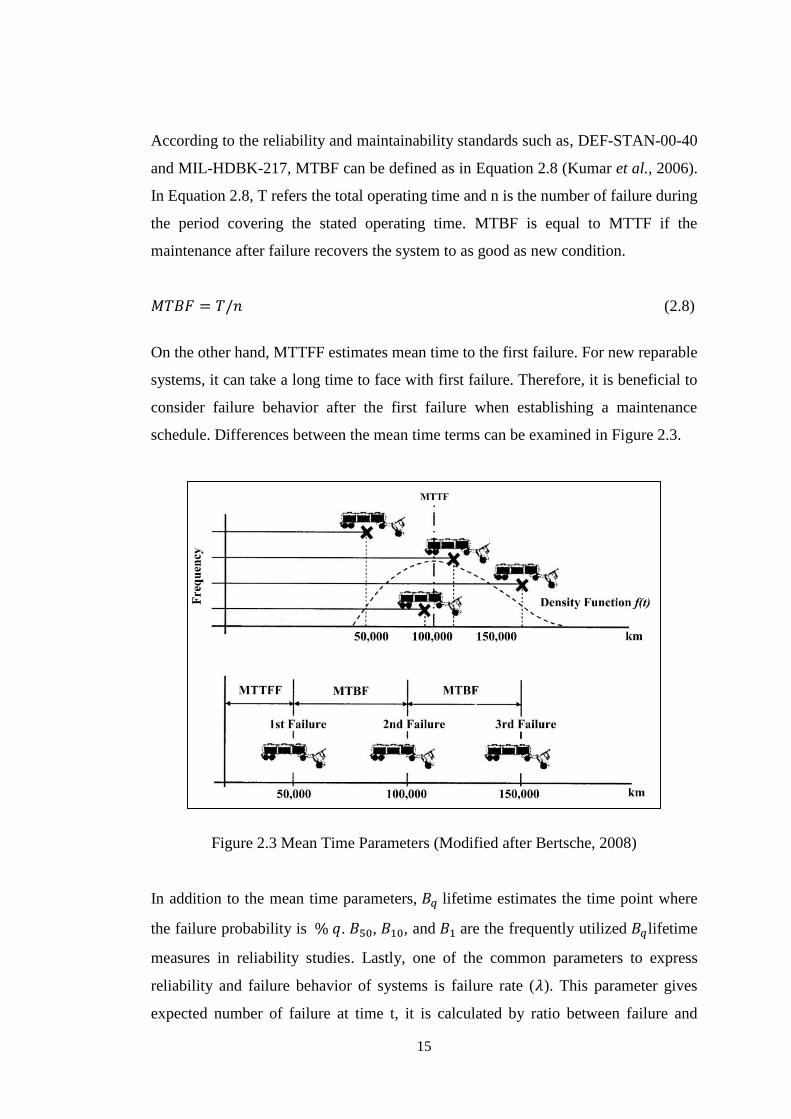
schedule. Differences between the mean time terms can be examined in Figure 2.3.

Figure 2.3 Mean Time Parameters (Modified after Bertsche, 2008)

In addition to the mean time parameters, 𝐵𝑞 lifetime estimates the time point where

the failure probability is % 𝑞. 𝐵50, 𝐵10, and 𝐵1 are the frequently utilized 𝐵𝑞lifetime

measures in reliability studies. Lastly, one of the common parameters to express

reliability and failure behavior of systems is failure rate (𝜆). This parameter gives

expected number of failure at time t, it is calculated by ratio between failure and

16

survival probabilities, 𝑓(𝑡)/𝑅(𝑡). Cumulative failure (hazard) rate, i.e. 𝐻(𝑡), in an

interval can be obtained using Equation 2.9 (Kumar et al., 2006).

𝐻(𝑡) = ∫ 𝜆(𝑥)𝑡

0𝑑𝑥 (2.9)

2.3.2 System Reliability Analysis

System is a combination of subsystems which carry out separate tasks under a

common-target working structure. Reliability analysis can be performed to examine

failure behavior of whole system or only specified subsystems. Each subsystem can

be regarded as an individual system by itself.

Reliability studies are handled in two groups as repairable and non-repairable ones.

Non-repairable systems cannot be restored after failures and they are placed with the

new ones. Best-fit distributions are utilized to investigate the time-dependent

reliabilities of these systems. On the other hand, repairable systems are the systems

that can be returned into functional states after failures via repairing activities.

Repairable systems can include non-repairable components or subsystems. For

instance, an individual light bulb is non-repairable system. However, a traffic light

mechanism is a repairable system which holds three non-repairable signal lights. In

this sense, mining equipment and machines can be considered as repairable systems.

In recent decades, various methods have been improved and modified for investigation

of repairable system reliability. These methods intend to evaluate reliability in both

qualitative and quantitative measures. Reliability block diagrams, fault tree analysis,

Markov process, and renewal process can be utilized to evaluate system reliability

quantitatively where failure modes and effects analysis, result process analysis, design

reviews, check list, and fault tree analysis are common in qualitative reliability analysis

(Bertsche, 2008). This section only focuses on reliability block diagrams, failure

modes and effects analysis, fault tree analysis, and Markov process. Renewal process

will be discussed in Section 2.5.

17

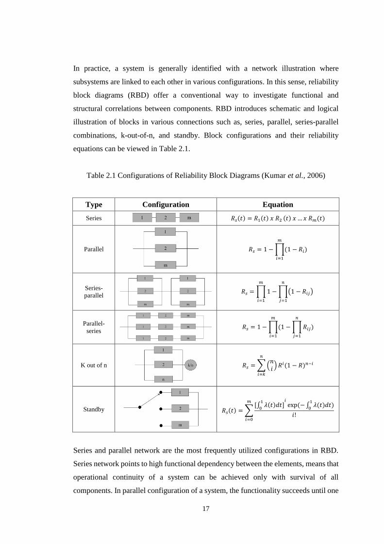
In practice, a system is generally identified with a network illustration where

subsystems are linked to each other in various configurations. In this sense, reliability

block diagrams (RBD) offer a conventional way to investigate functional and

structural correlations between components. RBD introduces schematic and logical

illustration of blocks in various connections such as, series, parallel, series-parallel

combinations, k-out-of-n, and standby. Block configurations and their reliability

equations can be viewed in Table 2.1.

Table 2.1 Configurations of Reliability Block Diagrams (Kumar et al., 2006)

Type Configuration Equation

Series 𝑅𝑠(𝑡) = 𝑅1(𝑡) 𝑥 𝑅2 (𝑡) 𝑥 … 𝑥 𝑅𝑚(𝑡)

Parallel

𝑅𝑠 = 1 − ∏(1 − 𝑅𝑖)

𝑚

𝑖=1

Series-

parallel

𝑅𝑠 = ∏ 1 − ∏(1 − 𝑅𝑖𝑗)

𝑛

𝑗=1

𝑚

𝑖=1

Parallel-

series

𝑅𝑠 = 1 − ∏(1 − ∏ 𝑅𝑖𝑗

𝑛

𝑗=1

)

𝑚

𝑖=1

K out of n

𝑅𝑠 = ∑ (𝑛𝑖

)

𝑛

𝑖=𝑘

𝑅𝑖(1 − 𝑅)𝑛−𝑖

Standby

𝑅𝑠(𝑡) = ∑[∫ 𝜆(𝑡)𝑑𝑡]

1

0

𝑖exp (− ∫ 𝜆(𝑡)𝑑𝑡)

1

0

𝑖!

𝑚

𝑖=0

Series and parallel network are the most frequently utilized configurations in RBD.

Series network points to high functional dependency between the elements, means that

operational continuity of a system can be achieved only with survival of all

components. In parallel configuration of a system, the functionality succeeds until one

18

component remains to operate. Parallel network indicates that interruptions due to

failure of any component can be compensated with another working component. In

addition, system can be configured in combination of series and parallel networks as

series-parallel and parallel-series as given in Table 2.1.

Moreover, one special configuration is k-out-of-n network utilized for the system

where at least k out of n units should work for operability of the system. This working

condition means that functionality of n-k failed components can be tolerated by k

surviving components. K-out-of-n system can be identified as in Table 2.1 if all

components are identical and functionally independent.

Another configuration in RBD is standby network, also called as redundant systems.

In this system, one unit works while other units are hold in standby condition. In case

of failure, standby unit starts to operate instead of the failed unit. If no delay is assumed

during transition from the failed unit to the standby one and all units are identical,

equation in Table 2.1 can be utilized.

In addition to RBD, Failure modes and effects analysis (FMEA) is another common

qualitative methods in system reliability investigation. It is utilized to describe,

analyze, and document the potential failure modes that can occur within a system and

the effects of those failures on the system efficiency (Murthy et al., 2008). If FMEA

also includes criticality analysis for failure modes, the method is called as Failure

Modes, Effects, and Criticality Analysis (FMECA). Differently from FMEA, FMECA

allows to examine system reliability quantitatively. This criticality analysis uses two

methods, (i) Risk Priority Number (RPN) utilized in industrial areas commonly. It uses

ranking values for failure occurrence, severity, and detection and (ii) military standard

technique with code of MIL-STD-1629 which is performed in high-security areas such

as, military defense, aerospace, and nuclear plants with ranking the criticality of failure

modes (Stapelberg, 2009).

FMEA aims to form a perspective to comprehend all causes of failure modes and

resultant effects on operability of components and systems. Qualitative evaluation

using FMEA is generally achieved answering the following questions (Murthy et al.,

19

2008): (i) What is the probability of component failure modes to occur? (ii) Which

interactions might cause failure modes? (iii) What are the resultant effects of the

probable failures? (iv) How might the failures be detected? (v) What are the ways to

prevent these failures at early stages?

FMEA is an informative process covering definition of the functions, definition of the

functional failure, determination and assignment of the failure modes for the failures,

and effects of the failure modes on the mechanism (Marquez, 2007). Before initiating

the process, symptom, mode, cause, and effect should be well-defined (Smith, 2007).

Failure symptom is an early indicator of approaching failure. However, some failures

may suddenly appear without revealing any symptom in many cases. Secondly, failure

mode answers the question “what is wrong?”. Failure modes can be described in

various ways, e.g. bent, ruptured, sheared, cracked, and frayed. In addition, failure

cause investigates the underlying reasons of failures. Lastly, failure effect describes

the potential consequences of the failure.

FMEA might be classified into three groups due to application area as design-level

FMEA, system-level FMEA, and process-level FMEA (Ireson et al., 1995). Design-

level analysis concerns about the parametric validity of product design by identifying

failure modes for components in subsystems and evaluating via alternative design

ways to improve the reliability of system design. System-level FMEA interests in

hierarchical system assessment in the preliminary product design to minimize failure

risk. Lastly, process-level analysis deals with the prevention and description of

potential failures in fabrication and assembly stages.

Another reliability assessment method, fault tree analysis (FTA) presents deductive

and systematical system reliability assessment using graphical illustrations to

symbolize internal and external reliability considerations of system elements. It gives

opportunity to evaluate system reliability both qualitatively and quantitatively. This

structured method was first developed by Bell Laboratories in corporation with Boing

and American Air Force to identify all potential risks of an unintentional launch of

ballistic missile between 1950 and 1960 (Berk, 2009). Then, it was started to be

20

utilized extensively for critical and complex systems especially in aerospace and

nuclear industries.

This analysis method covers logical, systematic, and effective attitude to realize the

weaknesses of pre-defined top event with employing top-to-down definition structure

(Kumar et al., 2006). Fault tree does not evaluate all failure modes in the system if

they are irrelevant of the top event. Deductive nature of the process conveniently

reveals the effectiveness of sub-events on the top event. Developing a FTA starts with

identification of top event and proceeds with assignment of down-events using

interaction symbols.

Symbols used in FTA can be grouped as events, gates, and transfer symbols (Berk,

2009). Events symbolize the incidents themselves that occur and cause the failures.

They can be classified as command event, basic failure event, normal event, human

error or undeveloped event, and condition event. Command event is in rectangle shape

and it refers the incident originated from its down-events, i.e. basic failure events.

These basic failure events are illustrated with circle and they present how the command

event can fail. Normal events are house shape and they indicate the events normally

expected to occur. Their probabilities are fixed and take the binary values, i.e. 1 or 0.

Human error or undeveloped event is diamond shape. Human error is a failure event

due to the operational or technical errors of working staff. On the other hand,

undeveloped events are considered as basic failure events that don not require further

solution. Condition event is in ellipsoid shape and it shows the restriction or inhibiting

condition that can be applied to any gate.

In addition to the events, gates point to the relationships between the events. AND gate

and OR gate are the most frequently utilized gates to define component dependencies

in systems. AND gate means that failure of one event depends on the occurrence of all

sub-events. On the other hand, OR operator states that occurrence of at least one input

event is enough for the occurrence of the output event. There are also some special

gates such as, voting (k-out-of-n), inhibit, priority AND, and XOR. Voting gate

symbolizes the cases where at least k out of n input events should take place for the

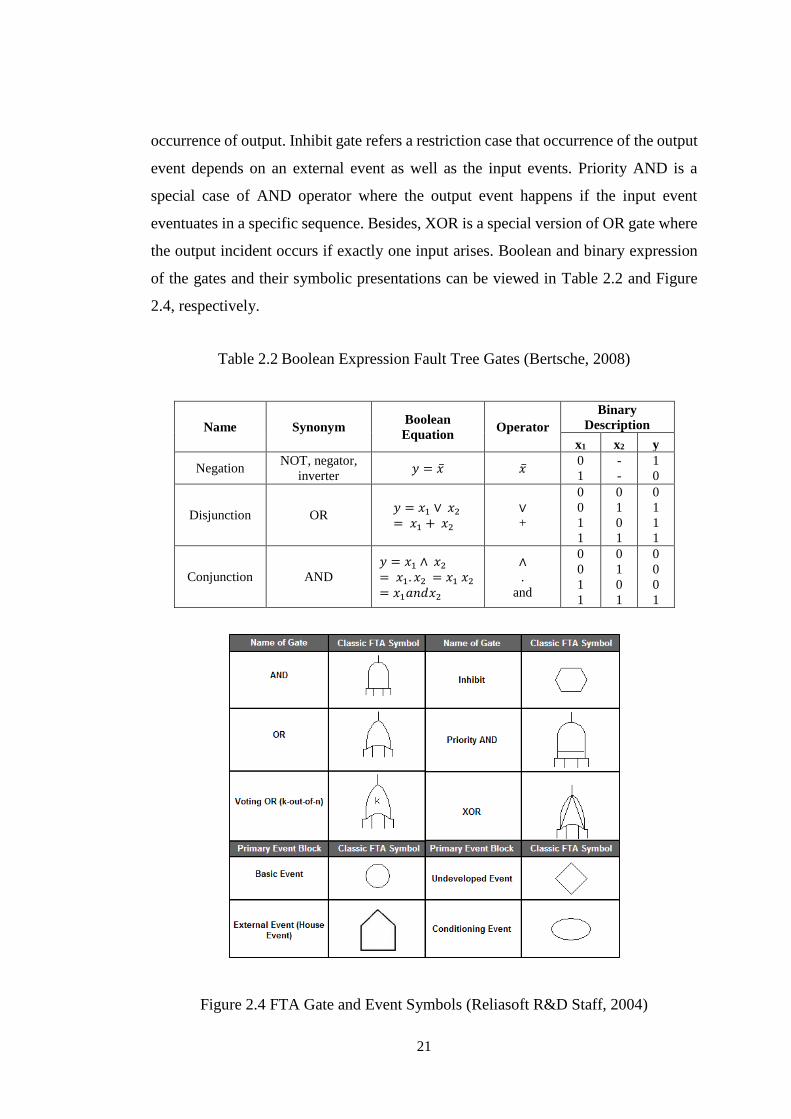
21

occurrence of output. Inhibit gate refers a restriction case that occurrence of the output

event depends on an external event as well as the input events. Priority AND is a

special case of AND operator where the output event happens if the input event

eventuates in a specific sequence. Besides, XOR is a special version of OR gate where

the output incident occurs if exactly one input arises. Boolean and binary expression

of the gates and their symbolic presentations can be viewed in Table 2.2 and Figure

2.4, respectively.

Table 2.2 Boolean Expression Fault Tree Gates (Bertsche, 2008)

Name Synonym Boolean

Equation Operator

Binary

Description

x1 x2 y

Negation NOT, negator,

inverter 𝑦 = �̅� �̅�

0

1

-

-

1

0

Disjunction OR 𝑦 = 𝑥1 ∨ 𝑥2

= 𝑥1 + 𝑥2

∨

+

0

0

1

1

0

1

0

1

0

1

1

1

Conjunction AND

𝑦 = 𝑥1 ∧ 𝑥2

= 𝑥1. 𝑥2 = 𝑥1 𝑥2

= 𝑥1𝑎𝑛𝑑𝑥2

∧

.

and

0

0

1

1

0

1

0

1

0

0

0

1

Figure 2.4 FTA Gate and Event Symbols (Reliasoft R&D Staff, 2004)

22

The last reliability method, Markov analysis is a memoryless stochastic process to

determine the probabilistic behavior of the systems in future using the present working

state (Marquez, 2007). This stochastic analysis is free of past behavior of system and

only utilizes its present state and age (Kumar et al., 2006). Assumptions in Markov

analysis are (Shooman, 1990):

(i) Failure and repair rates utilized as transition rate are kept constant. It means that

Markov method defines failure and repair behaviors with exponential

distribution.

(ii) Components are independent of each other.

(iii) Probabilistic transition of one system state in Δt time is stated as λΔt or μΔ,

where λ and μ are failure and repair rates respectively.

(iv) Probability of more than one transition in Δt time is ignored.

Markov analysis can work with discrete or continuous space of states and time.

Discrete state and discrete time-based Markov analysis is called as Markov chain while

continuous state and continuous time-based Markov analysis is named as Markov

process (Marquez, 2007). In addition, system state and time can be discrete and

continuous or vice versa.

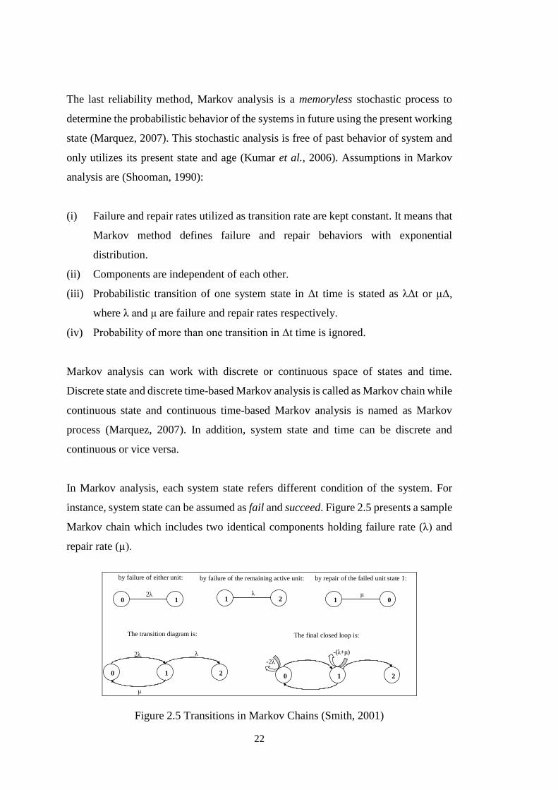
In Markov analysis, each system state refers different condition of the system. For

instance, system state can be assumed as fail and succeed. Figure 2.5 presents a sample

Markov chain which includes two identical components holding failure rate (λ) and

repair rate (µ).

0 1 1 2 1 02λ λ μ

0 1 2 0 1 2

2λ λ

μ

-2λ

-(λ+μ)

by failure of either unit: by failure of the remaining active unit: by repair of the failed unit state 1:

The final closed loop is:The transition diagram is:

Figure 2.5 Transitions in Markov Chains (Smith, 2001)

23

The states of system in Figure 2.5 can be donated as (i) State-0, succeed of both

components, (ii) State-1, one component operating other failed, and (iii) State-2, both

components failed. Mathematical expressions of Markov analysis for simple systems

and their derivative solutions can be investigated from Smith (2001).

2.4 Definition and Classification of Maintenance Activities

Maintenance can be identified as activities required to hold a system and its

subsystems in operational state and to keep sustainability of production while

minimizing operational cost (Stephens, 2010). Maintenance cost can be classified as

direct costs including physical expenses and indirect cost which is nonphysical

consequences of system halts due to maintenance. Amount of cost may reach to

substantial levels if downtime management of system fails and unplanned breakdowns

induce successive negative effects on system functionality. In addition, increasing

demand in industries and high-rate production cycle may raise failure frequency and

resultant costs. This condition forces sectors to develop more conservative and

preventive maintenance programs.

Portion of maintenance cost in operating cost of systems has raised dramatically in

recent decades. Only in 1981, $ 600 billion was spent for maintenance of substantial

plant systems in the USA and the amount was doubled in early 2000 (Mobley, 2004).

One third of the maintenance expenses were observed to be wasted due to insufficient

maintenance policies and/or techniques. In this sense, issues covering determination,

testing and confirmation of proper maintenance program particular to systems hold

vital importance for the longevity of the system operations. Maintainability, which is

a phenomenon to control planned and unplanned failures, basically aims to satisfy

system requirements to decrease factors such as, working hours, equipment, logistic

expenses, skill level, and service area (Dhillon, 1999). In this basis, the maintainability

defines a probabilistic approach considering spare part condition and maintenance

crew capacity, and also optimal time intervals for repairing and inspection (Bertsche,

2008). On the other hand, a maintenance policy defines how to implement corrective

and preventive activities with including also when and who questions.

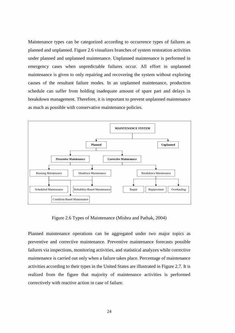
24

Maintenance types can be categorized according to occurrence types of failures as

planned and unplanned. Figure 2.6 visualizes branches of system restoration activities

under planned and unplanned maintenance. Unplanned maintenance is performed in

emergency cases when unpredictable failures occur. All effort in unplanned

maintenance is given to only repairing and recovering the system without exploring

causes of the resultant failure modes. In an unplanned maintenance, production

schedule can suffer from holding inadequate amount of spare part and delays in

breakdown management. Therefore, it is important to prevent unplanned maintenance

as much as possible with conservative maintenance policies.

MAINTENANCE SYSTEM

Planned Unplanned

Preventive Maintenance Corrective Maintenance

Running Maintenance Shutdown Maintenance

Scheduled Maintenance Reliability-Based Maintenance

Condition-Based Maintenance

Breakdown Maintenance

Repair Replacement Overhauling

Figure 2.6 Types of Maintenance (Mishra and Pathak, 2004)

Planned maintenance operations can be aggregated under two major topics as

preventive and corrective maintenance. Preventive maintenance forecasts possible

failures via inspections, monitoring activities, and statistical analyzes while corrective

maintenance is carried out only when a failure takes place. Percentage of maintenance

activities according to their types in the United States are illustrated in Figure 2.7. It is

realized from the figure that majority of maintenance activities is performed

correctively with reactive action in case of failure.

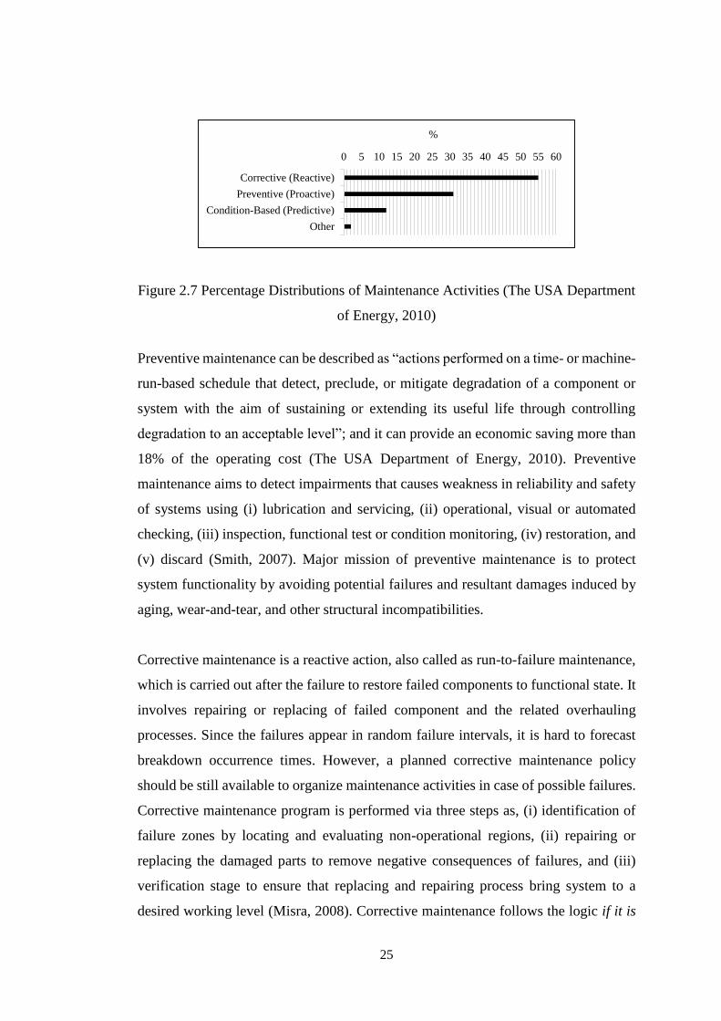
25

Figure 2.7 Percentage Distributions of Maintenance Activities (The USA Department

of Energy, 2010)

Preventive maintenance can be described as “actions performed on a time- or machine-

run-based schedule that detect, preclude, or mitigate degradation of a component or

system with the aim of sustaining or extending its useful life through controlling

degradation to an acceptable level”; and it can provide an economic saving more than

18% of the operating cost (The USA Department of Energy, 2010). Preventive

maintenance aims to detect impairments that causes weakness in reliability and safety

of systems using (i) lubrication and servicing, (ii) operational, visual or automated

checking, (iii) inspection, functional test or condition monitoring, (iv) restoration, and

(v) discard (Smith, 2007). Major mission of preventive maintenance is to protect

system functionality by avoiding potential failures and resultant damages induced by

aging, wear-and-tear, and other structural incompatibilities.

Corrective maintenance is a reactive action, also called as run-to-failure maintenance,

which is carried out after the failure to restore failed components to functional state. It

involves repairing or replacing of failed component and the related overhauling

processes. Since the failures appear in random failure intervals, it is hard to forecast

breakdown occurrence times. However, a planned corrective maintenance policy

should be still available to organize maintenance activities in case of possible failures.

Corrective maintenance program is performed via three steps as, (i) identification of

failure zones by locating and evaluating non-operational regions, (ii) repairing or

replacing the damaged parts to remove negative consequences of failures, and (iii)

verification stage to ensure that replacing and repairing process bring system to a

desired working level (Misra, 2008). Corrective maintenance follows the logic if it is

0 5 10 15 20 25 30 35 40 45 50 55 60

Corrective (Reactive)

Preventive (Proactive)

Condition-Based (Predictive)

Other

%

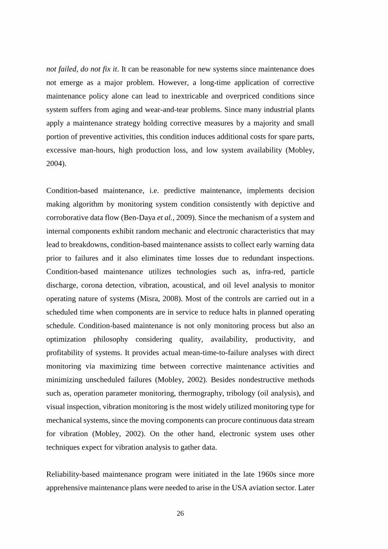
26

not failed, do not fix it. It can be reasonable for new systems since maintenance does

not emerge as a major problem. However, a long-time application of corrective

maintenance policy alone can lead to inextricable and overpriced conditions since

system suffers from aging and wear-and-tear problems. Since many industrial plants

apply a maintenance strategy holding corrective measures by a majority and small

portion of preventive activities, this condition induces additional costs for spare parts,

excessive man-hours, high production loss, and low system availability (Mobley,

2004).

Condition-based maintenance, i.e. predictive maintenance, implements decision

making algorithm by monitoring system condition consistently with depictive and

corroborative data flow (Ben-Daya et al., 2009). Since the mechanism of a system and

internal components exhibit random mechanic and electronic characteristics that may

lead to breakdowns, condition-based maintenance assists to collect early warning data

prior to failures and it also eliminates time losses due to redundant inspections.

Condition-based maintenance utilizes technologies such as, infra-red, particle

discharge, corona detection, vibration, acoustical, and oil level analysis to monitor

operating nature of systems (Misra, 2008). Most of the controls are carried out in a

scheduled time when components are in service to reduce halts in planned operating

schedule. Condition-based maintenance is not only monitoring process but also an

optimization philosophy considering quality, availability, productivity, and

profitability of systems. It provides actual mean-time-to-failure analyses with direct

monitoring via maximizing time between corrective maintenance activities and

minimizing unscheduled failures (Mobley, 2002). Besides nondestructive methods

such as, operation parameter monitoring, thermography, tribology (oil analysis), and

visual inspection, vibration monitoring is the most widely utilized monitoring type for

mechanical systems, since the moving components can procure continuous data stream

for vibration (Mobley, 2002). On the other hand, electronic system uses other

techniques expect for vibration analysis to gather data.

Reliability-based maintenance program were initiated in the late 1960s since more

apprehensive maintenance plans were needed to arise in the USA aviation sector. Later

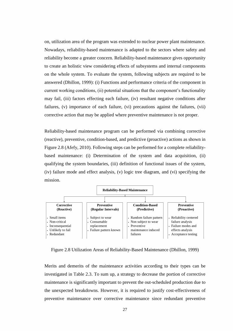
27

on, utilization area of the program was extended to nuclear power plant maintenance.

Nowadays, reliability-based maintenance is adapted to the sectors where safety and

reliability become a greater concern. Reliability-based maintenance gives opportunity

to create an holistic view considering effects of subsystems and internal components

on the whole system. To evaluate the system, following subjects are required to be

answered (Dhillon, 1999): (i) Functions and performance criteria of the component in

current working conditions, (ii) potential situations that the component’s functionality

may fail, (iii) factors effecting each failure, (iv) resultant negative conditions after

failures, (v) importance of each failure, (vi) precautions against the failures, (vii)

corrective action that may be applied where preventive maintenance is not proper.

Reliability-based maintenance program can be performed via combining corrective

(reactive), preventive, condition-based, and predictive (proactive) actions as shown in

Figure 2.8 (Afefy, 2010). Following steps can be performed for a complete reliability-

based maintenance: (i) Determination of the system and data acquisition, (ii)

qualifying the system boundaries, (iii) definition of functional issues of the system,

(iv) failure mode and effect analysis, (v) logic tree diagram, and (vi) specifying the

mission.

Reliability-Based Maintenance

Corrective

(Reactive)

Small items

Non-critical

Inconsequential

Unlikely to fail

Redundant

Preventive

(Regular Intervals)

Subject to wear

Consumable

replacement

Failure pattern known

Condition-Based

(Predictive)

Random failure pattern

Non subject to wear

Preventive

maintenance induced

failures

Preventive

(Proactive)

Reliability centered

failure analysis

Failure modes and

effects analysis

Acceptance testing

Figure 2.8 Utilization Areas of Reliability-Based Maintenance (Dhillon, 1999)

Merits and demerits of the maintenance activities according to their types can be

investigated in Table 2.3. To sum up, a strategy to decrease the portion of corrective

maintenance is significantly important to prevent the out-scheduled production due to

the unexpected breakdowns. However, it is required to justify cost-effectiveness of

preventive maintenance over corrective maintenance since redundant preventive

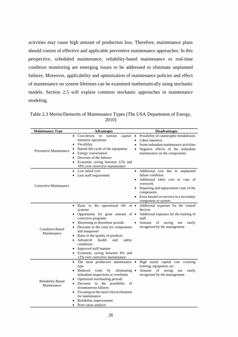
28

activities may cause high amount of production loss. Therefore, maintenance plans

should consist of effective and applicable preventive maintenance approaches. In this

perspective, scheduled maintenance, reliability-based maintenance or real-time

condition monitoring are emerging issues to be addressed to eliminate unplanned

failures. Moreover, applicability and optimization of maintenance policies and effect

of maintenance on system lifetimes can be examined mathematically using stochastic

models. Section 2.5 will explain common stochastic approaches in maintenance

modeling.

Table 2.3 Merits/Demerits of Maintenance Types (The USA Department of Energy,

2010)

Maintenance Type Advantages Disadvantages

Preventive Maintenance

Cost-driven in various capital-

intensive operations

Flexibility

Raised life-cycle of the equipment

Energy conversation

Decrease of the failures

Economic saving between 12% and

18% over corrective maintenance

Possibility of catastrophic breakdowns

Labor-intensive

Some redundant maintenance activities

Negative effects of the redundant

maintenance on the components

Corrective Maintenance

Low initial cost

Less staff requirement

Additional cost due to unplanned

failure condition

Additional labor cost in case of

overwork

Repairing and replacement costs of the

components

Extra hazard occurrence in a secondary

component or system

Condition-Based

Maintenance

Raise in the operational life of

systems

Opportunity for great amount of

corrective programs

Shortening in downtime periods

Decrease in the costs for components

and manpower

Raise in the quality of products

Advanced health and safety

conditions

Improved staff manner

Economic saving between 8% and

12% over corrective maintenance

Additional expenses for the control

devices

Additional expenses for the training of

staff

Amount of saving not easily

recognized by the management

Reliability-Based

Maintenance

The most productive maintenance

type

Reduced costs by eliminating

redundant inspections or overhauls

Optimized overhauling periods

Decrease in the possibility of

instantaneous failures

Focusing on the most critical elements

for maintenance

Reliability improvement

Root cause analysis

High initial capital cost covering

training, equipment, etc.

Amount of saving not easily

recognized by the management

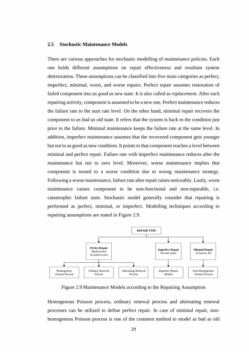
29

2.5 Stochastic Maintenance Models

There are various approaches for stochastic modelling of maintenance policies. Each

one holds different assumptions on repair effectiveness and resultant system

deterioration. These assumptions can be classified into five main categories as perfect,

imperfect, minimal, worst, and worse repairs. Perfect repair assumes restoration of

failed component into as good as new state. It is also called as replacement. After each

repairing activity, component is assumed to be a new one. Perfect maintenance reduces

the failure rate to the start rate level. On the other hand, minimal repair recovers the

component to as bad as old state. It refers that the system is back to the condition just

prior to the failure. Minimal maintenance keeps the failure rate at the same level. In

addition, imperfect maintenance assumes that the recovered component gets younger

but not to as good as new condition. It points to that component reaches a level between

minimal and perfect repair. Failure rate with imperfect maintenance reduces after the

maintenance but not to zero level. Moreover, worse maintenance implies that

component is turned to a worse condition due to wrong maintenance strategy.

Following a worse maintenance, failure rate after repair raises noticeably. Lastly, worst

maintenance causes component to be non-functional and non-reparable, i.e.

catastrophic failure state. Stochastic model generally consider that repairing is

performed as perfect, minimal, or imperfect. Modelling techniques according to

repairing assumptions are stated in Figure 2.9.

REPAIR TYPE

Perfect Repair

Replacement

As good as new

Imperfect Repair

Normal repair

Minimal Repair

As bad as old

Homogenous

Poisson Process

Ordinary Renewal

Process

Alternating Renewal

Process

Imperfect Repair

Models

Non-Homogenous

Poisson Process

Figure 2.9 Maintenance Models according to the Repairing Assumption

Homogenous Poisson process, ordinary renewal process and alternating renewal

processes can be utilized to define perfect repair. In case of minimal repair, non-

homogenous Poisson process is one of the common method to model as bad as old

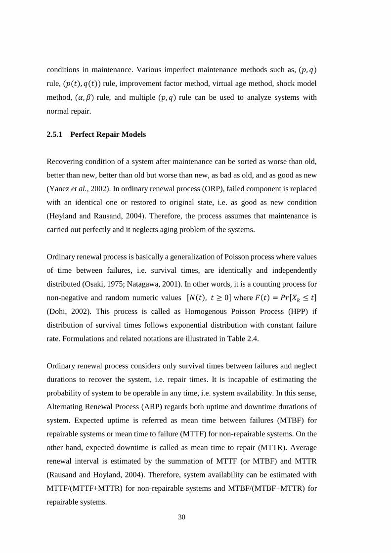
30

conditions in maintenance. Various imperfect maintenance methods such as, (𝑝, 𝑞)

rule, (𝑝(𝑡), 𝑞(𝑡)) rule, improvement factor method, virtual age method, shock model

method, (𝛼, 𝛽) rule, and multiple (𝑝, 𝑞) rule can be used to analyze systems with

normal repair.

2.5.1 Perfect Repair Models

Recovering condition of a system after maintenance can be sorted as worse than old,

better than new, better than old but worse than new, as bad as old, and as good as new

(Yanez et al., 2002). In ordinary renewal process (ORP), failed component is replaced

with an identical one or restored to original state, i.e. as good as new condition

(Høyland and Rausand, 2004). Therefore, the process assumes that maintenance is

carried out perfectly and it neglects aging problem of the systems.

Ordinary renewal process is basically a generalization of Poisson process where values

of time between failures, i.e. survival times, are identically and independently

distributed (Osaki, 1975; Natagawa, 2001). In other words, it is a counting process for

non-negative and random numeric values [𝑁(𝑡), 𝑡 ≥ 0] where 𝐹(𝑡) = 𝑃𝑟[𝑋𝑘 ≤ 𝑡]

(Dohi, 2002). This process is called as Homogenous Poisson Process (HPP) if

distribution of survival times follows exponential distribution with constant failure

rate. Formulations and related notations are illustrated in Table 2.4.

Ordinary renewal process considers only survival times between failures and neglect

durations to recover the system, i.e. repair times. It is incapable of estimating the

probability of system to be operable in any time, i.e. system availability. In this sense,

Alternating Renewal Process (ARP) regards both uptime and downtime durations of

system. Expected uptime is referred as mean time between failures (MTBF) for

repairable systems or mean time to failure (MTTF) for non-repairable systems. On the

other hand, expected downtime is called as mean time to repair (MTTR). Average

renewal interval is estimated by the summation of MTTF (or MTBF) and MTTR

(Rausand and Hoyland, 2004). Therefore, system availability can be estimated with

MTTF/(MTTF+MTTR) for non-repairable systems and MTBF/(MTBF+MTTR) for

repairable systems.

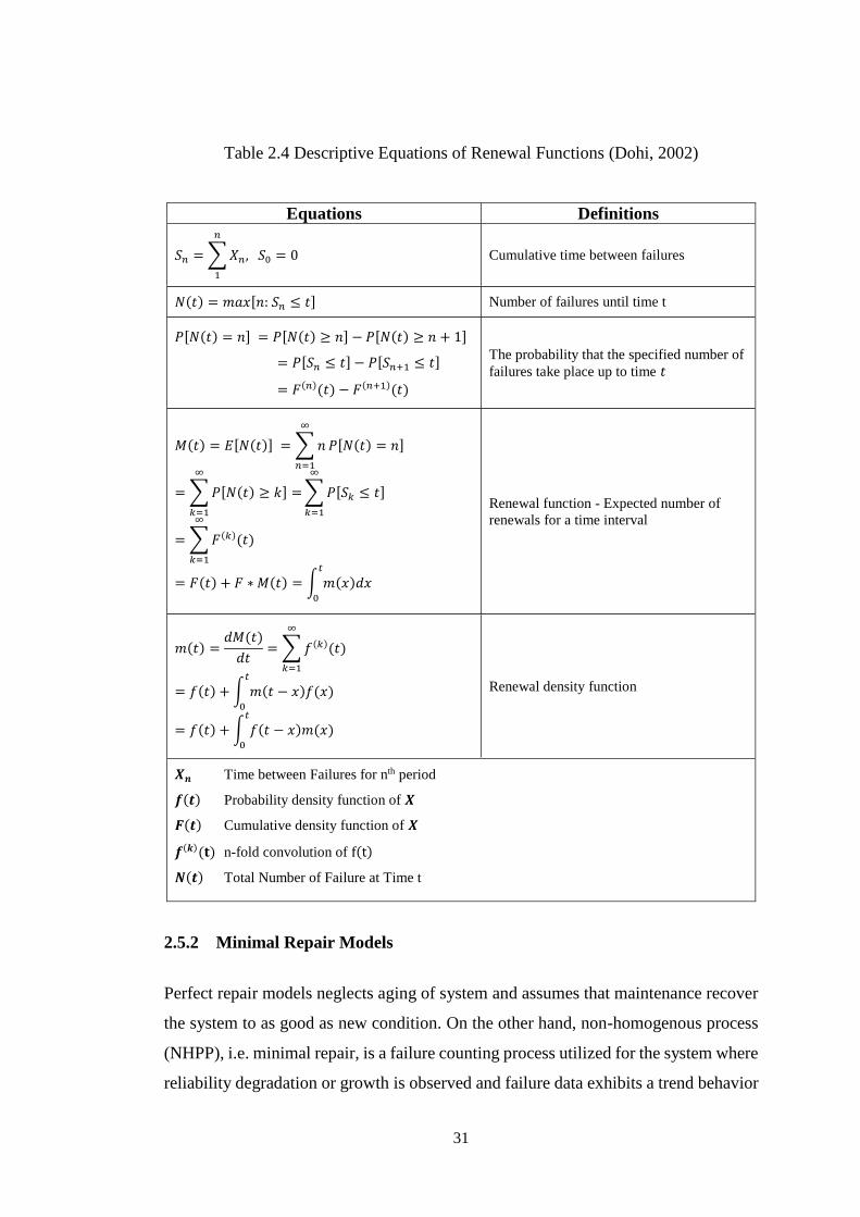
31

Table 2.4 Descriptive Equations of Renewal Functions (Dohi, 2002)

Equations Definitions

𝑆𝑛 = ∑ 𝑋𝑛, 𝑆0 = 0

𝑛

1

Cumulative time between failures

𝑁(𝑡) = 𝑚𝑎𝑥[𝑛: 𝑆𝑛 ≤ 𝑡] Number of failures until time t

𝑃[𝑁(𝑡) = 𝑛] = 𝑃[𝑁(𝑡) ≥ 𝑛] − 𝑃[𝑁(𝑡) ≥ 𝑛 + 1]

= 𝑃[𝑆𝑛 ≤ 𝑡] − 𝑃[𝑆𝑛+1 ≤ 𝑡]

= 𝐹(𝑛)(𝑡) − 𝐹(𝑛+1)(𝑡)

The probability that the specified number of

failures take place up to time 𝑡

𝑀(𝑡) = 𝐸[𝑁(𝑡)] = ∑ 𝑛

∞

𝑛=1

𝑃[𝑁(𝑡) = 𝑛]

= ∑ 𝑃[𝑁(𝑡) ≥ 𝑘] =

∞

𝑘=1

∑ 𝑃[𝑆𝑘 ≤ 𝑡]

∞

𝑘=1

= ∑ 𝐹(𝑘)(𝑡)

∞

𝑘=1

= 𝐹(𝑡) + 𝐹 ∗ 𝑀(𝑡) = ∫ 𝑚(𝑥)𝑑𝑥𝑡

0

Renewal function - Expected number of

renewals for a time interval

𝑚(𝑡) =𝑑𝑀(𝑡)

𝑑𝑡= ∑ 𝑓(𝑘)(𝑡)

∞

𝑘=1

= 𝑓(𝑡) + ∫ 𝑚(𝑡 − 𝑥)𝑓(𝑥)𝑡

0

= 𝑓(𝑡) + ∫ 𝑓(𝑡 − 𝑥)𝑚(𝑥)𝑡

0

Renewal density function

𝑿𝒏 Time between Failures for nth period

𝒇(𝒕) Probability density function of 𝑿

𝑭(𝒕) Cumulative density function of 𝑿

𝒇(𝒌)(𝐭) n-fold convolution of f(t)

𝑵(𝒕) Total Number of Failure at Time t

2.5.2 Minimal Repair Models

Perfect repair models neglects aging of system and assumes that maintenance recover

the system to as good as new condition. On the other hand, non-homogenous process

(NHPP), i.e. minimal repair, is a failure counting process utilized for the system where

reliability degradation or growth is observed and failure data exhibits a trend behavior

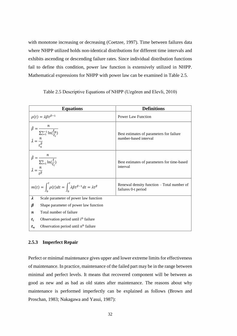
32

with monotone increasing or decreasing (Coetzee, 1997). Time between failures data

where NHPP utilized holds non-identical distributions for different time intervals and

exhibits ascending or descending failure rates. Since individual distribution functions

fail to define this condition, power law function is extensively utilized in NHPP.

Mathematical expressions for NHPP with power law can be examined in Table 2.5.

Table 2.5 Descriptive Equations of NHPP (Uzgören and Elevli, 2010)

Equations Definitions

𝜌(𝑡) = 𝜆𝛽𝑡𝛽−1 Power Law Function

�̂� =𝑛

∑ ln (𝑡𝑛

𝑡𝑖

𝑛−1𝑖=1 )

�̂� =𝑛

𝑡𝑛�̂�

Best estimates of parameters for failure

number-based interval

�̂� =𝑛

∑ ln (𝑡𝑡𝑖

𝑛𝑖=1 )

�̂� =𝑛

𝑡�̂�

Best estimates of parameters for time-based

interval

𝑚(𝑡) = ∫ 𝜌(𝑡)𝑑𝑡𝑡

0

= ∫ 𝜆𝛽𝑡𝛽−1𝑑𝑡𝑡

0

= 𝜆𝑡𝛽 Renewal density function – Total number of

failures 0-t period

𝝀 Scale parameter of power law function

𝜷 Shape parameter of power law function

𝒏 Total number of failure

𝒕𝒊 Observation period until ith failure

𝒕𝒏 Observation period until nth failure

2.5.3 Imperfect Repair

Perfect or minimal maintenance gives upper and lower extreme limits for effectiveness

of maintenance. In practice, maintenance of the failed part may be in the range between

minimal and perfect levels. It means that recovered component will be between as

good as new and as bad as old states after maintenance. The reasons about why

maintenance is performed imperfectly can be explained as follows (Brown and

Proschan, 1983; Nakagawa and Yasui, 1987):

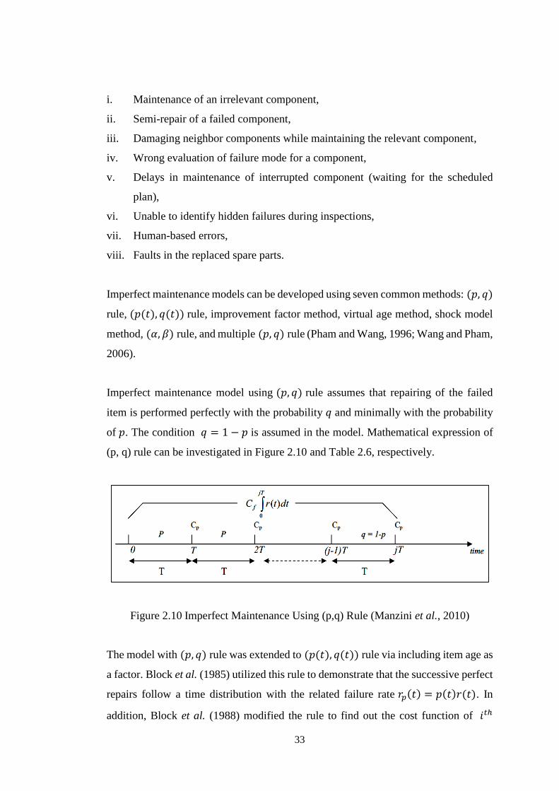
33

i. Maintenance of an irrelevant component,

ii. Semi-repair of a failed component,

iii. Damaging neighbor components while maintaining the relevant component,

iv. Wrong evaluation of failure mode for a component,

v. Delays in maintenance of interrupted component (waiting for the scheduled

plan),

vi. Unable to identify hidden failures during inspections,

vii. Human-based errors,

viii. Faults in the replaced spare parts.

Imperfect maintenance models can be developed using seven common methods: (𝑝, 𝑞)

rule, (𝑝(𝑡), 𝑞(𝑡)) rule, improvement factor method, virtual age method, shock model

method, (𝛼, 𝛽) rule, and multiple (𝑝, 𝑞) rule (Pham and Wang, 1996; Wang and Pham,

2006).

Imperfect maintenance model using (𝑝, 𝑞) rule assumes that repairing of the failed

item is performed perfectly with the probability 𝑞 and minimally with the probability

of 𝑝. The condition 𝑞 = 1 − 𝑝 is assumed in the model. Mathematical expression of

(p, q) rule can be investigated in Figure 2.10 and Table 2.6, respectively.

Figure 2.10 Imperfect Maintenance Using (p,q) Rule (Manzini et al., 2010)

The model with (𝑝, 𝑞) rule was extended to (𝑝(𝑡), 𝑞(𝑡)) rule via including item age as

a factor. Block et al. (1985) utilized this rule to demonstrate that the successive perfect

repairs follow a time distribution with the related failure rate 𝑟𝑝(𝑡) = 𝑝(𝑡)𝑟(𝑡). In

addition, Block et al. (1988) modified the rule to find out the cost function of 𝑖𝑡ℎ

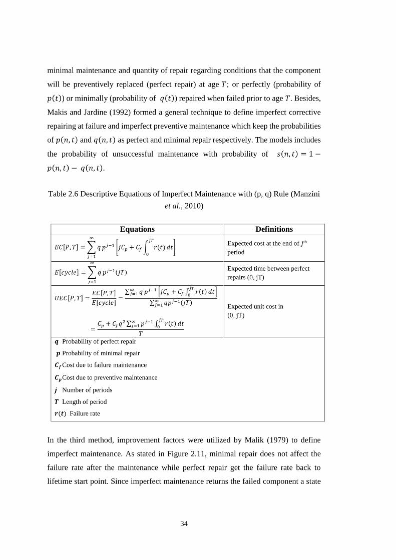
34

minimal maintenance and quantity of repair regarding conditions that the component

will be preventively replaced (perfect repair) at age 𝑇; or perfectly (probability of

𝑝(𝑡)) or minimally (probability of 𝑞(𝑡)) repaired when failed prior to age 𝑇. Besides,

Makis and Jardine (1992) formed a general technique to define imperfect corrective

repairing at failure and imperfect preventive maintenance which keep the probabilities

of 𝑝(𝑛, 𝑡) and 𝑞(𝑛, 𝑡) as perfect and minimal repair respectively. The models includes

the probability of unsuccessful maintenance with probability of 𝑠(𝑛, 𝑡) = 1 −

𝑝(𝑛, 𝑡) − 𝑞(𝑛, 𝑡).

Table 2.6 Descriptive Equations of Imperfect Maintenance with (p, q) Rule (Manzini

et al., 2010)

Equations Definitions

𝐸𝐶[𝑃, 𝑇] = ∑ 𝑞

∞

𝑗=1

𝑝𝑗−1 [𝑗𝐶𝑝 + 𝐶𝑓 ∫ 𝑟(𝑡)𝑗𝑇

0

𝑑𝑡] Expected cost at the end of 𝑗th

period

𝐸[𝑐𝑦𝑐𝑙𝑒] = ∑ 𝑞

∞

𝑗=1

𝑝𝑗−1(𝑗𝑇) Expected time between perfect

repairs (0, jT)

𝑈𝐸𝐶[𝑃, 𝑇] =𝐸𝐶[𝑃, 𝑇]

𝐸[𝑐𝑦𝑐𝑙𝑒]=

∑ 𝑞∞𝑗=1 𝑝𝑗−1 [𝑗𝐶𝑝 + 𝐶𝑓 ∫ 𝑟(𝑡)

𝑗𝑇

0𝑑𝑡]

∑ 𝑞𝑝𝑗−1(𝑗𝑇)∞𝑗=1

=𝐶𝑝 + 𝐶𝑓𝑞2 ∑ 𝑝𝑗−1∞

𝑗=1 ∫ 𝑟(𝑡)𝑗𝑇

0𝑑𝑡

𝑇

Expected unit cost in

(0, jT)

𝒒 Probability of perfect repair

𝒑 Probability of minimal repair

𝑪𝒇 Cost due to failure maintenance

𝑪𝒑 Cost due to preventive maintenance

𝒋 Number of periods

𝑻 Length of period

𝒓(𝒕) Failure rate

In the third method, improvement factors were utilized by Malik (1979) to define

imperfect maintenance. As stated in Figure 2.11, minimal repair does not affect the

failure rate after the maintenance while perfect repair get the failure rate back to

lifetime start point. Since imperfect maintenance returns the failed component a state

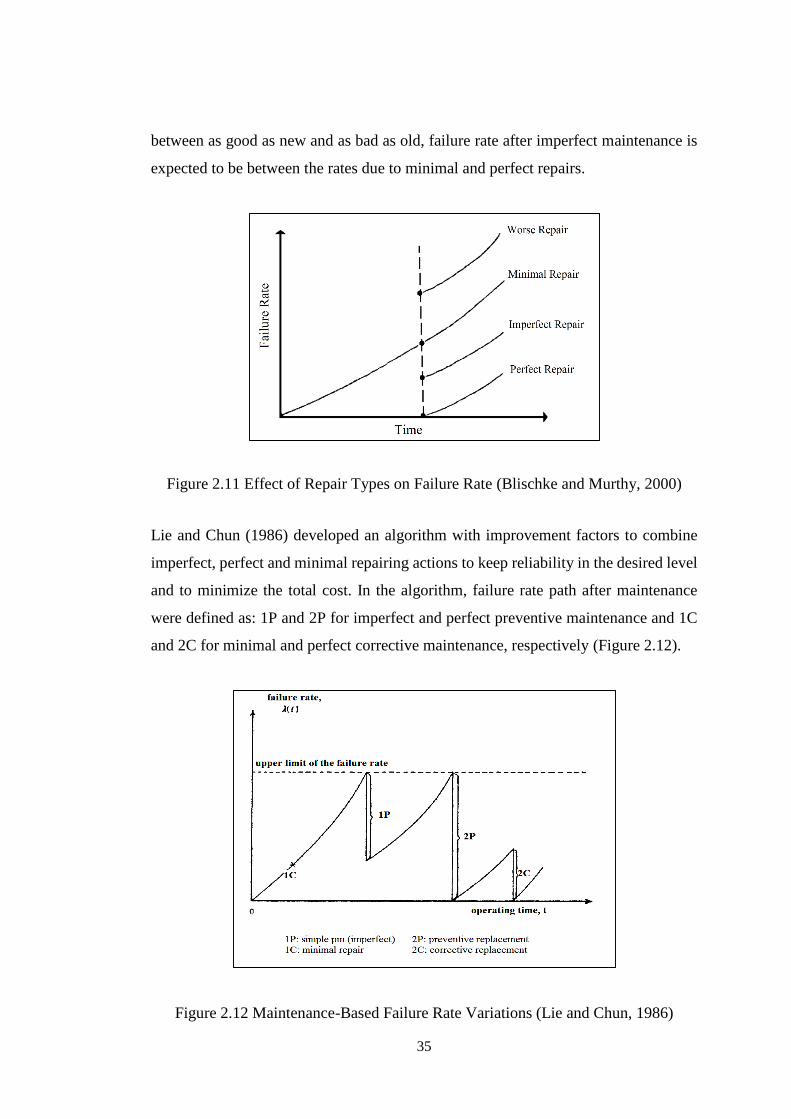
35

between as good as new and as bad as old, failure rate after imperfect maintenance is

expected to be between the rates due to minimal and perfect repairs.

Figure 2.11 Effect of Repair Types on Failure Rate (Blischke and Murthy, 2000)

Lie and Chun (1986) developed an algorithm with improvement factors to combine

imperfect, perfect and minimal repairing actions to keep reliability in the desired level

and to minimize the total cost. In the algorithm, failure rate path after maintenance

were defined as: 1P and 2P for imperfect and perfect preventive maintenance and 1C

and 2C for minimal and perfect corrective maintenance, respectively (Figure 2.12).

Figure 2.12 Maintenance-Based Failure Rate Variations (Lie and Chun, 1986)

36

The forth model for building an imperfect maintenance methodology is virtual age

method by Kijima et al. (1988). The proposed model assumes that system age

increases depending on the repair improvement factor. It means that if the repair is

performed perfectly, no aging is seen between the (𝑛)𝑡ℎ and (𝑛 − 1)𝑡ℎ repair (Tadj et

al., 2011). Virtual age of a system was defined with two separate models by Kijima et

al. (1988). In the first model, it is supposed that (𝑛)𝑡ℎ repair eliminates the damage

only between (𝑛)𝑡ℎ and (𝑛 − 1)𝑡ℎ repairs. If the time elapsed between this time point

is defined as 𝑋𝑛 = 𝑡𝑛 − 𝑡𝑛−1, virtual age for Model-I can be expressed as in Equation

2.10. In the equation, 𝑉𝑛−1 is the virtual age prior to the (𝑛 − 1)𝑡ℎ repairs and 𝐴𝑛

(also denoted as 𝑞 or 𝐴 in some studies) is the improvement factor (also referred as

restoration factor, degree of repair).

𝑉𝑛 = 𝑉𝑛−1 + 𝐴𝑛𝑋𝑛 (2.10)

Equation 2.10 indicates that maintenance improvements only effect time period

between maintenance activities and it does not offer a general recovery on whole

lifetime. On the other hand, Kijima Model-II assumes that maintenance recovers

cumulative damage loss in system instead of the damage only in an exact period.

Equation 2.11 shows the formula related to Model-II.

𝑉𝑛 = 𝐴𝑛(𝑉𝑛−1 + 𝑋𝑛) (2.11)

Equation 2.11 reveals the effect of improvement factor on increasing lifetime of

system. In this sense, improvement after maintenance does not concern only a small

period between two maintenance point but also effect overall cumulative lifetime.

Shock model is another common method for imperfect maintenance. The model

basically considers the accumulating damages on the item that may cause failure when

the limits are exceeded (Nakagawa, 2007). Successive shocks on item may cause

deterioration. Even, sudden shocks may result in catastrophic failure of component. In

this sense, preventive maintenance supports component health by keeping the

cumulative loss under the limit values. Kijima and Nakagawa (1991) used shock model

37

to measure the percentage of damage reduction due to the preventive maintenance. It

is assumed that the preventive maintenance decreases the addictive shock (damage) by

100 (1 − 𝑏)% where 𝑏 = 1 refers the minimal repair and 𝑏 = 0 means perfect

repair. In addition, Finkelstein (1998) combined virtual age and shock models to

examine the probabilities of shocks to induce failure. The study covered various

models for minimal, perfect, and general (imperfect) maintenance.

Sixth model of imperfect maintenance modelling is quasi-renewal process, also called

as (𝛼, 𝛽) rule. Model assumes that survival times between the failures will decrease

with rate of 𝛼 due to system aging and repair time will rise with rate of 𝛽 ,

proportionally. Inter-arrival times can be defined in terms of nonnegative random

variables, 𝑋𝑛 , as {𝑋1 = 𝑍1, 𝑋2 = 𝛼𝑍2, 𝑋3 = 𝛼2𝑍3, … } (Wang, 2008). It is obvious

that If 𝛼 = 1, then the process is reduced to ordinary renewal process. The conditions

of 𝛼 < 1 and 𝛼 > 1 points to decreasing and increasing quasi-renewal processes,

respectively.

The last model used to identify imperfect maintenance is multiple (𝑝, 𝑞) rule. This

model (Shaked and Shanthikumar, 1986; Sheu and Griffith, 1992) considers functional

dependencies between components. Therefore, joint distribution functions were

utilized to describe the dependency regarding the (𝑝, 𝑞) rule where 𝑝 and 𝑞 refer

perfect and minimal repair probabilities, respectively.

2.6 Optimization of Maintenance Policies

Maintenance policies organize all maintenance activities to be applied during

operational periods of systems. These policies decide the strategies for failure

conditions, preventive replacements, and inspections via clarifying questions of who,

how, when, and how long. Concept and complexity of a maintenance policy change

due to factors such as, number of components in systems, dependencies between

components, economic variables, capacity of maintenance crew, spare part conditions,

and administrative decisions. Maintenance policies should be developed in cost-

effective manner considering all negative and positive contributions of maintenance

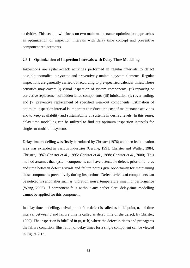
38

activities. This section will focus on two main maintenance optimization approaches

as optimization of inspection intervals with delay time concept and preventive

component replacements.

2.6.1 Optimization of Inspection Intervals with Delay-Time Modelling

Inspections are system-check activities performed in regular intervals to detect

possible anomalies in systems and preventively maintain system elements. Regular

inspections are generally carried out according to pre-specified calendar times. These

activities may cover: (i) visual inspection of system components, (ii) repairing or

corrective replacement of hidden failed components, (iii) lubrication, (iv) overhauling,

and (v) preventive replacement of specified wear-out components. Estimation of

optimum inspection interval is important to reduce unit cost of maintenance activities

and to keep availability and sustainability of systems in desired levels. In this sense,

delay time modelling can be utilized to find out optimum inspection intervals for

single- or multi-unit systems.

Delay time modelling was firstly introduced by Christer (1976) and then its utilization

area was extended in various industries (Cerone, 1991; Christer and Waller, 1984;

Christer, 1987; Christer et al., 1995; Christer et al., 1998; Christer et al., 2000). This

method assumes that system components can have detectable defects prior to failures

and time between defect arrivals and failure points give opportunity for maintaining

these components preventively during inspections. Defect arrivals of components can

be noticed via anomalies such as, vibration, noise, temperature, smell, or performance

(Wang, 2008). If component fails without any defect alert, delay-time modelling

cannot be applied for this component.

In delay time modelling, arrival point of the defect is called as initial point, u, and time

interval between u and failure time is called as delay time of the defect, h (Christer,

1999). The inspection is fulfilled in (u, u+h) where the defect initiates and propagates

the failure condition. Illustration of delay times for a single component can be viewed

in Figure 2.13.

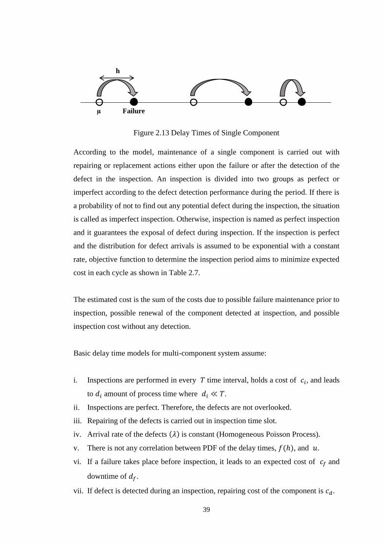
39

Figure 2.13 Delay Times of Single Component

According to the model, maintenance of a single component is carried out with

repairing or replacement actions either upon the failure or after the detection of the

defect in the inspection. An inspection is divided into two groups as perfect or

imperfect according to the defect detection performance during the period. If there is

a probability of not to find out any potential defect during the inspection, the situation

is called as imperfect inspection. Otherwise, inspection is named as perfect inspection

and it guarantees the exposal of defect during inspection. If the inspection is perfect

and the distribution for defect arrivals is assumed to be exponential with a constant

rate, objective function to determine the inspection period aims to minimize expected

cost in each cycle as shown in Table 2.7.

The estimated cost is the sum of the costs due to possible failure maintenance prior to

inspection, possible renewal of the component detected at inspection, and possible

inspection cost without any detection.

Basic delay time models for multi-component system assume:

i. Inspections are performed in every 𝑇 time interval, holds a cost of 𝑐𝑖, and leads

to 𝑑𝑖 amount of process time where 𝑑𝑖 ≪ 𝑇.

ii. Inspections are perfect. Therefore, the defects are not overlooked.

iii. Repairing of the defects is carried out in inspection time slot.

iv. Arrival rate of the defects (𝜆) is constant (Homogeneous Poisson Process).

v. There is not any correlation between PDF of the delay times, 𝑓(ℎ), and 𝑢.

vi. If a failure takes place before inspection, it leads to an expected cost of 𝑐𝑓 and

downtime of 𝑑𝑓.

vii. If defect is detected during an inspection, repairing cost of the component is 𝑐𝑑.

h

µ Failure

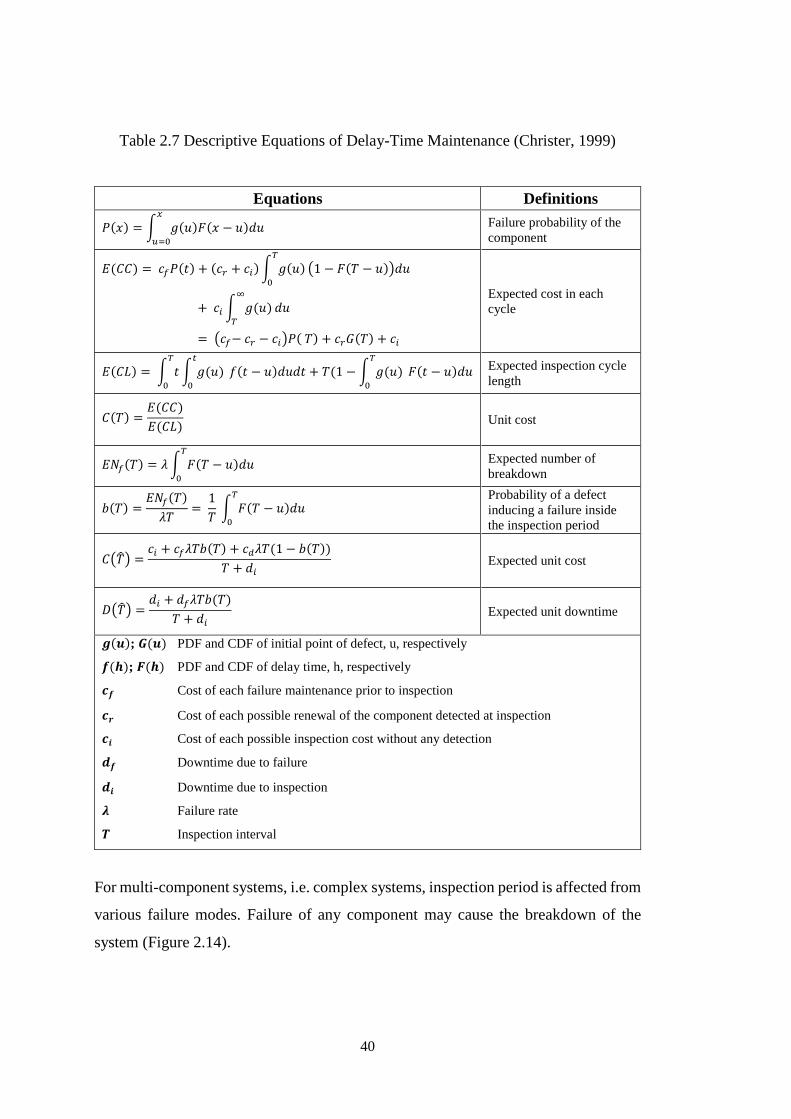
40

Table 2.7 Descriptive Equations of Delay-Time Maintenance (Christer, 1999)

Equations Definitions

𝑃(𝑥) = ∫ 𝑔(𝑢)𝐹(𝑥 − 𝑢)𝑑𝑢 𝑥

𝑢=0

Failure probability of the

component

𝐸(𝐶𝐶) = 𝑐𝑓𝑃(𝑡) + (𝑐𝑟 + 𝑐𝑖) ∫ 𝑔(𝑢)𝑇

0

(1 − 𝐹(𝑇 − 𝑢))𝑑𝑢

+ 𝑐𝑖 ∫ 𝑔(𝑢)∞

𝑇

𝑑𝑢

= (𝑐𝑓− 𝑐𝑟 − 𝑐𝑖)𝑃( 𝑇) + 𝑐𝑟𝐺(𝑇) + 𝑐𝑖

Expected cost in each

cycle

𝐸(𝐶𝐿) = ∫ 𝑡𝑇

0

∫ 𝑔(𝑢)𝑡

0

𝑓(𝑡 − 𝑢)𝑑𝑢𝑑𝑡 + 𝑇(1 − ∫ 𝑔(𝑢)𝑇

0

𝐹(𝑡 − 𝑢)𝑑𝑢 Expected inspection cycle

length

𝐶(𝑇) =𝐸(𝐶𝐶)

𝐸(𝐶𝐿) Unit cost

𝐸𝑁𝑓(𝑇) = 𝜆 ∫ 𝐹(𝑇 − 𝑢)𝑑𝑢𝑇

0

Expected number of

breakdown

𝑏(𝑇) =𝐸𝑁𝑓(𝑇)

𝜆𝑇=

1

𝑇 ∫ 𝐹(𝑇 − 𝑢)𝑑𝑢

𝑇

0

Probability of a defect

inducing a failure inside

the inspection period

𝐶(�̂�) =𝑐𝑖 + 𝑐𝑓𝜆𝑇𝑏(𝑇) + 𝑐𝑑𝜆𝑇(1 − 𝑏(𝑇))

𝑇 + 𝑑𝑖

Expected unit cost

𝐷(�̂�) =𝑑𝑖 + 𝑑𝑓𝜆𝑇𝑏(𝑇)

𝑇 + 𝑑𝑖

Expected unit downtime

𝒈(𝒖); 𝑮(𝒖) PDF and CDF of initial point of defect, u, respectively

𝒇(𝒉); 𝑭(𝒉) PDF and CDF of delay time, h, respectively

𝒄𝒇 Cost of each failure maintenance prior to inspection

𝒄𝒓 Cost of each possible renewal of the component detected at inspection

𝒄𝒊 Cost of each possible inspection cost without any detection

𝒅𝒇 Downtime due to failure

𝒅𝒊 Downtime due to inspection

𝝀 Failure rate

𝑻 Inspection interval

For multi-component systems, i.e. complex systems, inspection period is affected from

various failure modes. Failure of any component may cause the breakdown of the

system (Figure 2.14).

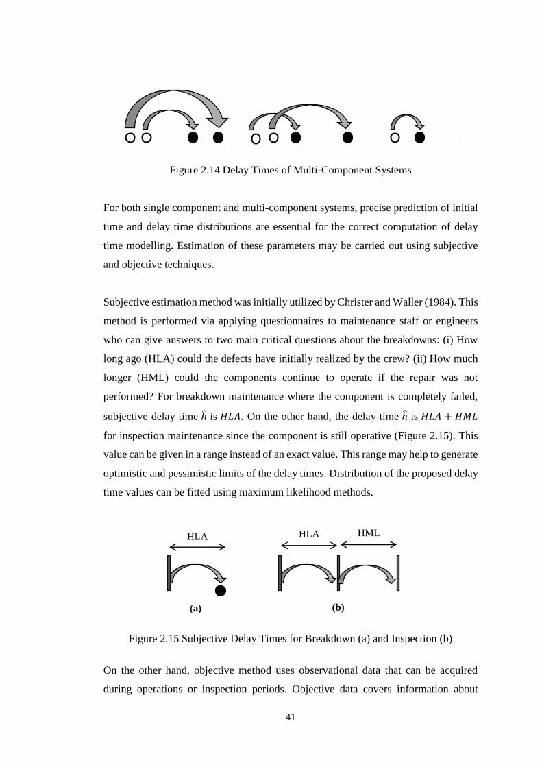
41

Figure 2.14 Delay Times of Multi-Component Systems

For both single component and multi-component systems, precise prediction of initial

time and delay time distributions are essential for the correct computation of delay

time modelling. Estimation of these parameters may be carried out using subjective

and objective techniques.

Subjective estimation method was initially utilized by Christer and Waller (1984). This

method is performed via applying questionnaires to maintenance staff or engineers

who can give answers to two main critical questions about the breakdowns: (i) How

long ago (HLA) could the defects have initially realized by the crew? (ii) How much

longer (HML) could the components continue to operate if the repair was not

performed? For breakdown maintenance where the component is completely failed,

subjective delay time ℎ̂ is 𝐻𝐿𝐴. On the other hand, the delay time ℎ̂ is 𝐻𝐿𝐴 + 𝐻𝑀𝐿

for inspection maintenance since the component is still operative (Figure 2.15). This

value can be given in a range instead of an exact value. This range may help to generate

optimistic and pessimistic limits of the delay times. Distribution of the proposed delay

time values can be fitted using maximum likelihood methods.

Figure 2.15 Subjective Delay Times for Breakdown (a) and Inspection (b)

On the other hand, objective method uses observational data that can be acquired

during operations or inspection periods. Objective data covers information about

HLA HML HLA

(a) (b)

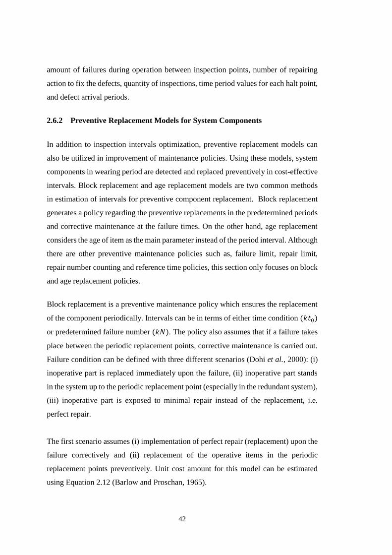
42

amount of failures during operation between inspection points, number of repairing

action to fix the defects, quantity of inspections, time period values for each halt point,

and defect arrival periods.

2.6.2 Preventive Replacement Models for System Components

In addition to inspection intervals optimization, preventive replacement models can

also be utilized in improvement of maintenance policies. Using these models, system

components in wearing period are detected and replaced preventively in cost-effective

intervals. Block replacement and age replacement models are two common methods

in estimation of intervals for preventive component replacement. Block replacement

generates a policy regarding the preventive replacements in the predetermined periods

and corrective maintenance at the failure times. On the other hand, age replacement

considers the age of item as the main parameter instead of the period interval. Although

there are other preventive maintenance policies such as, failure limit, repair limit,

repair number counting and reference time policies, this section only focuses on block

and age replacement policies.

Block replacement is a preventive maintenance policy which ensures the replacement

of the component periodically. Intervals can be in terms of either time condition (𝑘𝑡0)

or predetermined failure number (𝑘𝑁). The policy also assumes that if a failure takes

place between the periodic replacement points, corrective maintenance is carried out.

Failure condition can be defined with three different scenarios (Dohi et al., 2000): (i)

inoperative part is replaced immediately upon the failure, (ii) inoperative part stands

in the system up to the periodic replacement point (especially in the redundant system),

(iii) inoperative part is exposed to minimal repair instead of the replacement, i.e.

perfect repair.

The first scenario assumes (i) implementation of perfect repair (replacement) upon the

failure correctively and (ii) replacement of the operative items in the periodic

replacement points preventively. Unit cost amount for this model can be estimated

using Equation 2.12 (Barlow and Proschan, 1965).

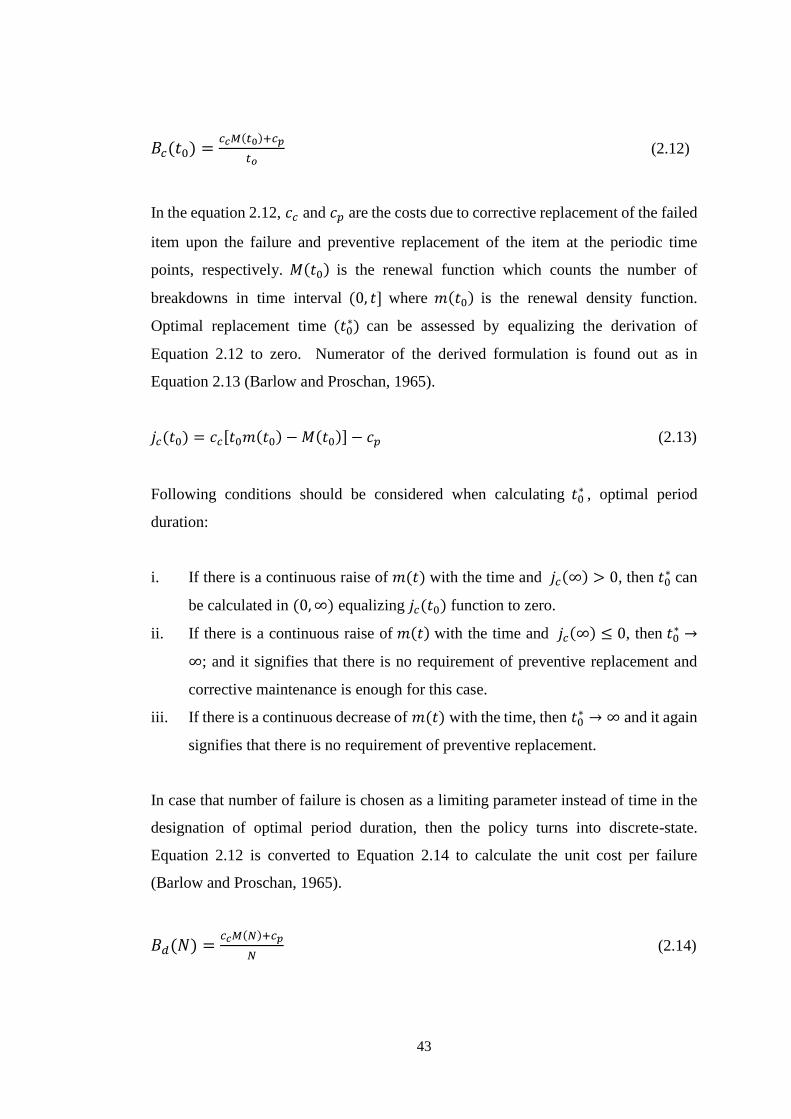
43

𝐵𝑐(𝑡0) =𝑐𝑐𝑀(𝑡0)+𝑐𝑝

𝑡𝑜 (2.12)

In the equation 2.12, 𝑐𝑐 and 𝑐𝑝 are the costs due to corrective replacement of the failed

item upon the failure and preventive replacement of the item at the periodic time

points, respectively. 𝑀(𝑡0) is the renewal function which counts the number of

breakdowns in time interval (0, 𝑡] where 𝑚(𝑡0) is the renewal density function.

Optimal replacement time (𝑡0∗) can be assessed by equalizing the derivation of

Equation 2.12 to zero. Numerator of the derived formulation is found out as in

Equation 2.13 (Barlow and Proschan, 1965).

𝑗𝑐(𝑡0) = 𝑐𝑐[𝑡0𝑚(𝑡0) − 𝑀(𝑡0)] − 𝑐𝑝 (2.13)

Following conditions should be considered when calculating 𝑡0∗ , optimal period

duration:

i. If there is a continuous raise of 𝑚(𝑡) with the time and 𝑗𝑐(∞) > 0, then 𝑡0∗ can

be calculated in (0, ∞) equalizing 𝑗𝑐(𝑡0) function to zero.

ii. If there is a continuous raise of 𝑚(𝑡) with the time and 𝑗𝑐(∞) ≤ 0, then 𝑡0∗ →

∞; and it signifies that there is no requirement of preventive replacement and

corrective maintenance is enough for this case.

iii. If there is a continuous decrease of 𝑚(𝑡) with the time, then 𝑡0∗ → ∞ and it again

signifies that there is no requirement of preventive replacement.

In case that number of failure is chosen as a limiting parameter instead of time in the

designation of optimal period duration, then the policy turns into discrete-state.

Equation 2.12 is converted to Equation 2.14 to calculate the unit cost per failure

(Barlow and Proschan, 1965).

𝐵𝑑(𝑁) =𝑐𝑐𝑀(𝑁)+𝑐𝑝

𝑁 (2.14)

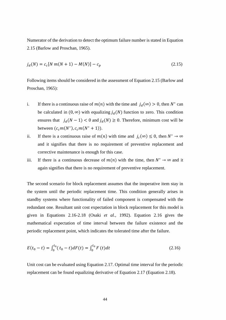
44

Numerator of the derivation to detect the optimum failure number is stated in Equation

2.15 (Barlow and Proschan, 1965).

𝑗𝑑(𝑁) = 𝑐𝑐[𝑁 𝑚(𝑁 + 1) − 𝑀(𝑁)] − 𝑐𝑝 (2.15)

Following items should be considered in the assessment of Equation 2.15 (Barlow and

Proschan, 1965):

i. If there is a continuous raise of 𝑚(𝑛) with the time and 𝑗𝑑(∞) > 0, then 𝑁∗ can

be calculated in (0, ∞) with equalizing 𝑗𝑑(𝑁) function to zero. This condition

ensures that 𝑗𝑑(𝑁 − 1) < 0 and 𝑗𝑑(𝑁) ≥ 0. Therefore, minimum cost will be

between (𝑐𝑐𝑚(𝑁∗), 𝑐𝑐𝑚(𝑁∗ + 1)).

ii. If there is a continuous raise of 𝑚(𝑛) with time and 𝑗𝑐(∞) ≤ 0, then 𝑁∗ → ∞

and it signifies that there is no requirement of preventive replacement and

corrective maintenance is enough for this case.

iii. If there is a continuous decrease of 𝑚(𝑛) with the time, then 𝑁∗ → ∞ and it

again signifies that there is no requirement of preventive replacement.

The second scenario for block replacement assumes that the inoperative item stay in

the system until the periodic replacement time. This condition generally arises in

standby systems where functionality of failed component is compensated with the

redundant one. Resultant unit cost expectation in block replacement for this model is

given in Equations 2.16-2.18 (Osaki et al., 1992). Equation 2.16 gives the

mathematical expectation of time interval between the failure existence and the

periodic replacement point, which indicates the tolerated time after the failure.

𝐸(𝑡0 − 𝑡) = ∫ (𝑡0

0𝑡0 − 𝑡)𝑑𝐹(𝑡) = ∫ 𝐹

𝑡0

0(𝑡)𝑑𝑡 (2.16)

Unit cost can be evaluated using Equation 2.17. Optimal time interval for the periodic

replacement can be found equalizing derivative of Equation 2.17 (Equation 2.18).

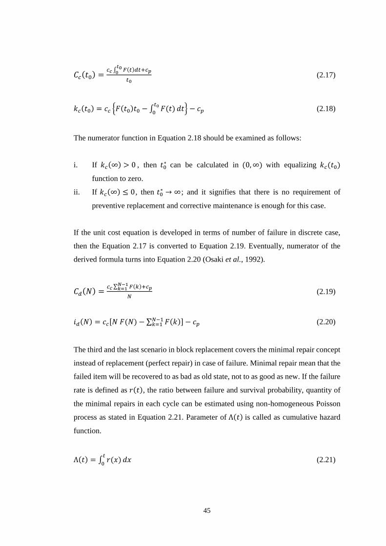
45

𝐶𝑐(𝑡0) =𝑐𝑐 ∫ 𝐹(𝑡)

𝑡00 𝑑𝑡+𝑐𝑝

𝑡0 (2.17)

𝑘𝑐(𝑡0) = 𝑐𝑐 {𝐹(𝑡0)𝑡0 − ∫ 𝐹(𝑡)𝑡0

0𝑑𝑡} − 𝑐𝑝 (2.18)

The numerator function in Equation 2.18 should be examined as follows:

i. If 𝑘𝑐(∞) > 0 , then 𝑡0∗ can be calculated in (0, ∞) with equalizing 𝑘𝑐(𝑡0)

function to zero.

ii. If 𝑘𝑐(∞) ≤ 0, then 𝑡0∗ → ∞; and it signifies that there is no requirement of

preventive replacement and corrective maintenance is enough for this case.

If the unit cost equation is developed in terms of number of failure in discrete case,

then the Equation 2.17 is converted to Equation 2.19. Eventually, numerator of the

derived formula turns into Equation 2.20 (Osaki et al., 1992).

𝐶𝑑(𝑁) =𝑐𝑐 ∑ 𝐹(𝑘)𝑁−1

𝑘=1 +𝑐𝑝

𝑁 (2.19)

𝑖𝑑(𝑁) = 𝑐𝑐[𝑁 𝐹(𝑁) − ∑ 𝐹(𝑘)𝑁−1𝑘=1 ] − 𝑐𝑝 (2.20)

The third and the last scenario in block replacement covers the minimal repair concept

instead of replacement (perfect repair) in case of failure. Minimal repair mean that the

failed item will be recovered to as bad as old state, not to as good as new. If the failure

rate is defined as 𝑟(𝑡), the ratio between failure and survival probability, quantity of

the minimal repairs in each cycle can be estimated using non-homogeneous Poisson

process as stated in Equation 2.21. Parameter of Λ(𝑡) is called as cumulative hazard

function.

Λ(𝑡) = ∫ 𝑟(𝑥)𝑡

0𝑑𝑥 (2.21)

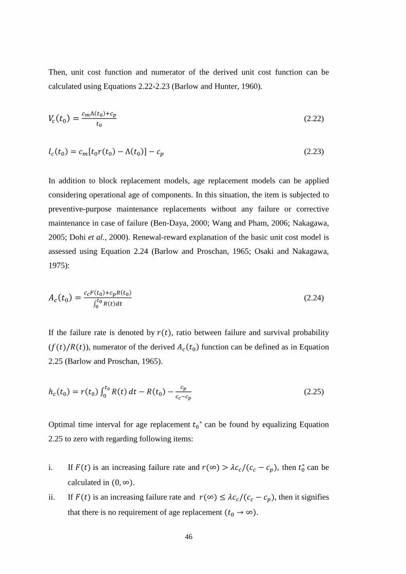
46

Then, unit cost function and numerator of the derived unit cost function can be

calculated using Equations 2.22-2.23 (Barlow and Hunter, 1960).

𝑉𝑐(𝑡0) =𝑐𝑚Λ(𝑡0)+𝑐𝑝

𝑡0 (2.22)

𝑙𝑐(𝑡0) = 𝑐𝑚[𝑡0𝑟(𝑡0) − Λ(𝑡0)] − 𝑐𝑝 (2.23)

In addition to block replacement models, age replacement models can be applied

considering operational age of components. In this situation, the item is subjected to

preventive-purpose maintenance replacements without any failure or corrective

maintenance in case of failure (Ben-Daya, 2000; Wang and Pham, 2006; Nakagawa,

2005; Dohi et al., 2000). Renewal-reward explanation of the basic unit cost model is

assessed using Equation 2.24 (Barlow and Proschan, 1965; Osaki and Nakagawa,

1975):

𝐴𝑐(𝑡0) =𝑐𝑐𝐹(𝑡0)+𝑐𝑝𝑅(𝑡0)

∫ 𝑅(𝑡)𝑡0

0 𝑑𝑡 (2.24)

If the failure rate is denoted by 𝑟(𝑡), ratio between failure and survival probability

(𝑓(𝑡)/𝑅(𝑡)), numerator of the derived 𝐴𝑐(𝑡0) function can be defined as in Equation

2.25 (Barlow and Proschan, 1965).

ℎ𝑐(𝑡0) = 𝑟(𝑡0) ∫ 𝑅(𝑡)𝑡0

0𝑑𝑡 − 𝑅(𝑡0) −

𝑐𝑝

𝑐𝑐−𝑐𝑝 (2.25)

Optimal time interval for age replacement 𝑡0∗ can be found by equalizing Equation

2.25 to zero with regarding following items:

i. If 𝐹(𝑡) is an increasing failure rate and 𝑟(∞) > 𝜆𝑐𝑐/(𝑐𝑐 − 𝑐𝑝), then 𝑡0∗ can be

calculated in (0, ∞).

ii. If 𝐹(𝑡) is an increasing failure rate and 𝑟(∞) ≤ 𝜆𝑐𝑐/(𝑐𝑐 − 𝑐𝑝), then it signifies

that there is no requirement of age replacement (𝑡0 → ∞).

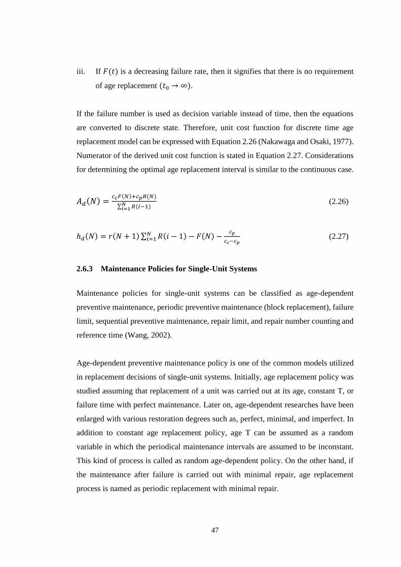
47

iii. If 𝐹(𝑡) is a decreasing failure rate, then it signifies that there is no requirement

of age replacement (𝑡0 → ∞).

If the failure number is used as decision variable instead of time, then the equations

are converted to discrete state. Therefore, unit cost function for discrete time age

replacement model can be expressed with Equation 2.26 (Nakawaga and Osaki, 1977).

Numerator of the derived unit cost function is stated in Equation 2.27. Considerations

for determining the optimal age replacement interval is similar to the continuous case.

𝐴𝑑(𝑁) =𝑐𝑐𝐹(𝑁)+𝑐𝑝𝑅(𝑁)

∑ 𝑅(𝑖−1)𝑁𝑖=1

(2.26)

ℎ𝑑(𝑁) = 𝑟(𝑁 + 1) ∑ 𝑅(𝑖 − 1)𝑁𝑖=1 − 𝐹(𝑁) −

𝑐𝑝

𝑐𝑐−𝑐𝑝 (2.27)

2.6.3 Maintenance Policies for Single-Unit Systems

Maintenance policies for single-unit systems can be classified as age-dependent

preventive maintenance, periodic preventive maintenance (block replacement), failure

limit, sequential preventive maintenance, repair limit, and repair number counting and

reference time (Wang, 2002).

Age-dependent preventive maintenance policy is one of the common models utilized

in replacement decisions of single-unit systems. Initially, age replacement policy was

studied assuming that replacement of a unit was carried out at its age, constant T, or

failure time with perfect maintenance. Later on, age-dependent researches have been

enlarged with various restoration degrees such as, perfect, minimal, and imperfect. In

addition to constant age replacement policy, age T can be assumed as a random

variable in which the periodical maintenance intervals are assumed to be inconstant.

This kind of process is called as random age-dependent policy. On the other hand, if

the maintenance after failure is carried out with minimal repair, age replacement

process is named as periodic replacement with minimal repair.

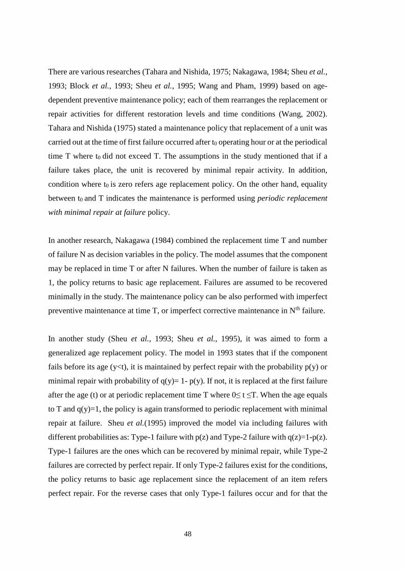
48

There are various researches (Tahara and Nishida, 1975; Nakagawa, 1984; Sheu et al.,

1993; Block et al., 1993; Sheu et al., 1995; Wang and Pham, 1999) based on age-

dependent preventive maintenance policy; each of them rearranges the replacement or

repair activities for different restoration levels and time conditions (Wang, 2002).

Tahara and Nishida (1975) stated a maintenance policy that replacement of a unit was

carried out at the time of first failure occurred after t0 operating hour or at the periodical

time T where t0 did not exceed T. The assumptions in the study mentioned that if a

failure takes place, the unit is recovered by minimal repair activity. In addition,

condition where t0 is zero refers age replacement policy. On the other hand, equality

between t0 and T indicates the maintenance is performed using periodic replacement

with minimal repair at failure policy.

In another research, Nakagawa (1984) combined the replacement time T and number

of failure N as decision variables in the policy. The model assumes that the component

may be replaced in time T or after N failures. When the number of failure is taken as

1, the policy returns to basic age replacement. Failures are assumed to be recovered

minimally in the study. The maintenance policy can be also performed with imperfect

preventive maintenance at time T, or imperfect corrective maintenance in Nth failure.

In another study (Sheu et al., 1993; Sheu et al., 1995), it was aimed to form a

generalized age replacement policy. The model in 1993 states that if the component

fails before its age (y<t), it is maintained by perfect repair with the probability p(y) or

minimal repair with probability of q(y)= 1- p(y). If not, it is replaced at the first failure

after the age (t) or at periodic replacement time T where 0≤ t ≤T. When the age equals

to T and q(y)=1, the policy is again transformed to periodic replacement with minimal

repair at failure. Sheu et al.(1995) improved the model via including failures with

different probabilities as: Type-1 failure with p(z) and Type-2 failure with q(z)=1-p(z).

Type-1 failures are the ones which can be recovered by minimal repair, while Type-2

failures are corrected by perfect repair. If only Type-2 failures exist for the conditions,

the policy returns to basic age replacement since the replacement of an item refers

perfect repair. For the reverse cases that only Type-1 failures occur and for that the

49

number of failures goes to infinity, policy is again called as periodic replacement with

minimal repair at failure.

Another age-dependent preventive maintenance policy called as repair replacement

policy was identified by Block et al. (1993). The study assumes preventive

replacement of survived unit at specified operating period or corrective repair of the

failed unit perfectly or minimally. The policy followed a conventional way where the

aging components are replaced with the identical one in specific time interval prior to

failures.

An alternative approach called as mixed age preventive maintenance policy was

studied by Wang and Pham (1999). In the study, it is assumed that component can be

exposed to two different failures after nth imperfect maintenance as: Type-1 which was

the total failure of the component requiring perfect (replacement) maintenance, and

Type-2 which was the failure that could be fixed by minimal repair. In addition, model

assumes that repair activity has a probability of p(y) to be performed as perfectly and

q(y)=1-p(y) as minimally. The period covering n imperfect repairing also meant

replacement age T. Therefore, the condition that equalizes the perfect repairing

probability and the number of imperfect repairing to zero reduced the model to

periodic replacement with minimal repair at failure. On the other hand, certain

existence of perfect repairing and lack of imperfect repairing transformed the model

to age replacement policy.

In addition to age-dependent preventive maintenance policy, other type of policy is

periodic preventive maintenance policy. It includes maintenance activities for certain

time intervals, kT. Block replacement policy is one of the common names utilized to

describe the replacement of a block or group in predetermined intervals. One approach

on periodic replacement with minimal repair at failure policy by Liu et al. (1995)

offered that the component would be replaced at time (O +1)T where O is the number

of imperfect preventive maintenance carried out in every T interval. On the other hand,

the model stated that possible failures between the intervals would be fixed by minimal

50

repair. It can be noted that if there is no any imperfect maintenance, the model reduces

to classic periodic replacement with minimal repair at failure policy.

An extended block replacement policy proposed by Berg and Epstein (1976) combined

the policy and age limitation. According to the model, replacement of the units with

ages less than or equal to the replacement period were kept working up to the failure

time or the replacement time. Failed components were replaced with the identical new

one. If the unit age is not less than periodic time interval, the model is turned to classic

block replacement policy.

Tango (1978) differentiated block replacement policy by suggesting that replacement

of the failed parts could be done with a used one as well as a new one. The failed

component was fixed by replacement with the new one when the failure took place

before the prescribed time limit. If the failure time was between the limit time and

periodic replacement time, a used spare part was utilized for the replacement.

Nakagawa (1981) modified periodic replacement with minimal repair at failure policy

via considering the possible after-failure strategies of the units. Periodic time length

was divided into two intervals as the period less than predetermined time point (T0)

and the period between this point and the periodic replacement time (T*). If the failure

exists before the predetermined time point (T0), maintenance is carried out with

minimal repair. Otherwise, in between T0 and T*, (policy-1) the failed part is not

maintained until the periodic time; or (policy-2) the failed part is replaced with the

spare one; or (policy-3) the failed part is replaced with the new one. If the

predetermined time point is taken as zero, policy-3 transforms to basic block

replacement policy.

In addition to age-dependent and periodic preventive maintenance policies, failure

limit, sequential preventive maintenance, repair limit, and repair number counting and

reference time are the other types of policies investigated in literature to regulate the

maintenance activity of single-unit systems. Failure limit policy can be used to

stabilize the failure rate and only carried out when the failures exceed the acceptable

51

limits due to the factors such as, wear and tear, fatigue or other age-based

consequences.

Sequential preventive maintenance policy assumes that the time periods for preventive

maintenance cannot be kept constant since the unit requires more frequent

maintenance due to its age. The models prepared with this approach are based on the

minimization of the cost for the next preventive maintenance. Nguyen and Murthy

(1981) proposed a policy predicating on the reference time point ti which was the

maximum operating time of unit without failure after (i-1)th repair activity. Also, the

component was indicated to be replaced after kth repair due to failure or at age ti,

whichever occurs initially. If k equals to zero, the model is turned to age replacement

policy.

Repair limit policy determines the limits between repairing and replacement activities.

The policy is divided into two approaches as repair cost limit policy and repair time

limit policy (Wang, 2002). Repair cost limit policy states that replacement of a unit

can be carried out if the predetermined cost limit is exceeded. On the other side, repair

time limit policy as defined by Nakagawa and Osaki (1974) restricts the repairing time

such that if the period exceed the limit, failed unit is replaced by the new one instead

of repairing.

The policies discussed in this section make various assumptions on scope and

boundary of the maintenance activities for single-unit systems. Maintenance manager

can choose one of these policies considering working mechanism of system and

applicability of the policy for the system.

2.6.4 Maintenance Policies for Multi-Unit Systems

Multi-unit systems cover more than one components in various combinations. If

maintenance of individual components is not applicable, maintenance policy for multi-

unit systems can be considered. Optimality of the maintenance should be assessed via

considering the dependencies between components. Opportunistic maintenance or

group maintenance policies can be utilized for multi-unit systems.

52

Opportunistic maintenance is applicable where the maintenance of one item gives

opportunity for repairing, inspection or replacement of the other items (Shenoy and

Bhadury, 2005). The phenomenon of opportunity may also rise when system is halted

due to demand reduction or other external reasons (Budai et al., 2008). There are

various researches investigating adaptation of opportunistic maintenance for different

modelling types. In this regard, Dekker and Smeitink (1991) implemented

opportunistic maintenance concept to block replacement policy. The model defined

the opportunity arrivals using renewal process. The study assumes that item

replacement is carried out correctively after the failure or preventively only when

opportunity arises. In addition, Dekker and Dijkstra (1992) used opportunistic

approach for age replacement, similar to block replacement model. Moreover, Cui and

Li (2006) extended imperfect shock model to opportunistic maintenance of multi-units

system.

On the other hand, group maintenance aims to gather items to be maintained

considering three common approaches as (i) replacement of items when any failure

occurs, (ii) placing redundant items into system design, and (iii) simultaneous

maintenance of the independent items which hold the same failure distribution (Wang

and Pham, 2006). For the stochastically compatible independent items, group policy

can be established using T-age replacement, m-failures replacement, and combination

of T-age and m-failures replacement (m,T) policies. Assaf and Shanthikumar (1987)

formed a group maintenance policy for a number of items having exponential PDFs.

The model assumed that the quantity of failures could be determined only in inspection

and repairing of the failed items was performed perfectly. Love et al. (1982) formed a

policy for a fleet of machine. Repair limit approach was applied in the model instead

of age and block maintenance types. It was assumed that replacement would only take

place only when the repair cost limit was exceeded. In another study, Gertsbakh (1989)

regarded the number of failure as a limit parameter to initiate the repairing activity.

Moreover, Sheu and Jhang (1997) introduced a model covering two phases for (0,T)

period and (T, T+W) period. The policy assumed that failure of the individual items

were repaired minimally in (0,T) and perfectly in (T, T+W). In the model, group

maintenance was only performed in (T, T+W).

53

2.7 Previous Reliability and Maintenance Studies in Mining

Mining is a machine-intensive sector where various mechanical systems are employed

in demanding working environments. They are exposed to various mechanical and

electrical failure modes during their lifetimes. These failures lead to time and

production losses and delay in production schedule. Maintenance cost of a machine

can reach a level between 35–60% of total operating cost in changing working

environments (Roy et al., 2001). Detection and control of prominent breakdowns and

developing predictive and preventive programs against failures are crucial for

longevity of machinery components and sustainability of machinery operations.

Draglines are massive earthmovers and sensitivity between machinery breakdowns

and production rate is extensively high for draglines. Research studies in the literature

are lack of maintenance optimization and component-based reliability modelling for

draglines. The existing dragline studies only offer general reliability models without

component decomposition and failure mode analysis. This section mentions about the

previous reliability and maintenance studies on mining systems.

Zhu et al. (1993) developed an artificial intelligence system called as Intelligent

Maintenance Support System (IMSS) gathering and interpreting data acquired from

sensors installed on the critical parts of trucks in an oil sand mine in Canada. The

system collected 47 variables through 21 analog and 26 digital signals with 30 minutes

intervals. The data was qualified using the knowledge base of experts, truck manuals

and data file. The authors claimed that IMSS gave apprehensible results for fault

diagnosis and condition monitoring.

Louit and Knights (2001) performed a discrete simulation to eliminate failures and

unplanned malfunction periods for the machine fleet of a gold-silver mine company in

Chile using root-cause failure analysis and generating repair standards. The research

aimed to reduce hidden costs due to accidents and delays in maintenance and to

increase the portion of planned maintenance. Concordantly, breakdown data collected

in the field was identified and quantified as planned and unplanned and delays in the

maintenance process were classified as lack of required personnel, lack of spare parts,

54

and priorities in the maintenance order. Simulations considered root-cause failure

analysis, modification in stock planning, repair standards, additional demand for labor

and workshop area, organizational changes, transferring of maintenance staff to

operation process, and maintenance contracting.

Veganes and Nuziale (2001) generated a genetic algorithm model for evaluation of

mining equipment reliability to reveal aging problem of component, operational

conditions, amount and quality of maintenance activities. The model was applied to

LHD, using information about failure types, values of time between failures, repair

periods, machine age, and the environmental conditions.

Roy et al. (2001) worked on the reliability and maintainability performance of four

electric rope shovels in India. In the study, shovel system was divided into twelve

subsystems. The analyses indicated that electrical and dipper subsystems were the

most critical subsystems considering repair durations and failure frequencies.

Lewis and Steinberg (2001) introduced an interactive maintenance management

system (IMMS) called as Intellimine which provided a real-time interface serving for

continuous data collection and analyses to get alarm about functional anomalies for

the machines. It was emphasized that maintenance cost was the greatest controllable

cost in the mining sector and 11% and 30% of the direct mining cost in the USA open

pits were due to the maintenance process and maintenance staff, respectively. In this

study, it was claimed that Intellimine presents a maintenance optimization interface

using the real-time data flow to control direct maintenance costs and indirect cost due

to production loss and redundant number of spare part and staff.

Samanta et al. (2004) carried out a research on reliability of LHD machinery system.

In the study, stochastic Markov process was utilized to measure the availability of

LHD as a function of reliability and maintenance. The system was divided into six

subsystems in serial connection so that failure in one unit could lead to a breakdown

of LHD. According to the analyses, transmission, drive unit, and hydraulic mechanism

55

of LHD were determined as the most problematic parts. Steady state availability of the

machine was estimated to be 73%.

Marquez (2005) aimed to build a simulation program intending for maintenance policy

assessment for truck engine to reduce total cumulative expected cost of maintenance.

Unit cost of failure due to expenses of employee, spare parts, rescheduled operations,

testing process, and responsible maintenance company were introduced in the model.

Simulation algorithm used semi-Markov process to evaluate the behavior of

maintenance policies in a continuous-time model.

Gupta et al. (2006) used fault tree approach to improve a logic-based reliability model

for longwall shearer. Any of the faults located in gear box, cutting drum, electric

motor, frame, ranging arm, power pack, and traction unit were supposed to induce

breakdown in the shearer. Reliability and functional importance of individual

components were evaluated using fault tree analysis.

Vagenas et al. (2007) summarized a methodology to determine reliability and

optimized maintenance intervals for LHD via combining analytical, statistical, and

graphical methods. Trend and serial correlation tests and goodness-of-fits of the

subsystem data for Weibull, exponential, and lognormal distributions was evaluated

using Kolmogorov-Smirnov and Chi-Squared tests. In the study, it was also stated that

Kolmogorov-Smirnov test was more convenient for non-normal distributions.

Barabady and Kumar (2008) focused on the reliability and availability factors of a

crushing plant in Jajarm Bauxite Mine of Iran using survival and repair data. The study

detected maintenance-critical subsystems with reliability importance factors. These

factors were estimated via time-dependent ratio between reliability of system and

component. In the study, the crushing plant was divided into six subsystems.

Individual lifetimes were estimated using best-fit distributions and non-homogenous

Poisson process for non-trend and trend components, respectively.

56

Uzgören et al. (2010) assessed the reliabilities of two draglines and estimated required

maintenance intervals for various reliability levels. Reliability assessment in the study

was carried out using best-fit distributions since there is not any indication of lifetime

trend. Mean time between the failures (MTBF) was found as 97.03 and 75.80 for

dragline-1 and dragline-2, respectively. Moreover, maintenance test released that

23.75 and 19.06 hours maintenance intervals were required to keep dragline-1 and

dragline-2 in 75% reliability level, respectively. Uzgören and Elevli (2010) also

applied non-homogenous Poisson process with power law to find out reliability of

draglines with lifetime trend behavior.

Hall and Daneshmend (2010) expressed data gathering and analysis procedures

frequently utilized in reliability analyses of mining machines. It was mentioned that

Pareto analysis, failure distribution interpretation, and repair time analysis were the

common methods in reliability estimations when adequate data was acquired from

sources such as, sensor, on-board interface in the equipment, historical failure data

sheet, and on-going maintenance and operation schedule. Application of failure mode

effects and criticality (FMECA) for small dataset was mentioned in the study.

Gölbaşı et al. (2013) explained how to decompose a dragline into subsystems and

components considering common failure modes existing in the mechanism. Failure

behaviors of draglines were investigated via comparing various bathtub curve

characteristics. In the study, variation of annual failure numbers and the resultant

downtimes for two draglines in Tunçbilek coal mine were also examined. Upper and

lower lifetime bounds of the subsystems for these draglines in 90% confidence interval

were estimated with reliability modelling.

Gölbaşı and Demirel (2013) investigated component failure behaviors of two draglines

currently operating in Tunçbilek coal mine via reliability importance factors and

assessed mean component availabilities. In this sense, twenty two components were

detected to induce failures in the draglines. Reliability variations of individual

components and their downtime profiles were utilized to determine expected

availabilities and expected failure numbers of the components at the end of 24th

57

operating hours. Regarding the degradation changes of component reliabilities, the

most critical components being prone to failure were detected.

Demirel et al. (2013) explained functional dependencies between dragline components

and system reliability variations using fault tree analysis. In this basis, dragline was

decomposed into seven subsystems as dragging, hoisting, rigging, bucket, movement,

machinery house, and boom. Following data classification to subsystems, data

anomalies were examined by run charts via controlling clustering, mixture, trend and

oscillation behaviors of successive data values. Time-dependent subsystem

reliabilities were calculated to estimate overall dragline reliability. Methodology of the

study was applied to the draglines in Tunçbilek coal mine.

Gölbaşı and Demirel (2015) made a review on quantitative and qualitative methods

that can be utilized to detect wear-out periods of mining machineries. Changes in

machinery failure rates throughout their lifetimes were discussed on a bathtub curve.

Qualitative trend tests such as, graph of cumulative failure numbers versus cumulative

time between failure and Duane plot were examined via numerical examples. Detailed

evaluation of quantitative trend tests such as, Crow-AMSAA, Laplace, Lewis-

Robincon, and reversal arrangement tests were investigated with a sample dataset.

Gölbaşı and Demirel (2015) performed a Monte Carlo simulation for two draglines to

reveal downtime profiles of the systems. In the study, trend behaviors for lifetime

datasets of individual components were observed using hypothesis testing methods,

Crow-AMSAA and Laplace. Lifetime characterizations of the components in either

lifetime growth or lifetime deterioration were evaluated with general renewal process.

Other components without lifetime trend were characterized using best-fit

distributions. Considering these assumptions, time-dependent failure rates of each

dragline subsystem were estimated. In addition, downtime profiles of the draglines

were determined using component lifetimes, random component repair times,

compulsory breaks due to regular inspections and legal shift breaks, and stochastic

behavior of energy source problems. Analyses showed that the dragline availabilities

changes between 64% and 69%.

58

2.8 Summary

This section presented an extensive literature survey on maintenance and reliability,

and their applications in mining sector. Factors contributing to system effectiveness

were also mentioned. The survey basically focus on reliability assessment methods

and maintenance policies. In this basis, reliability was discussed including descriptive

terms and system reliability methods. Maintenance issue was handled investigating

assumptions in maintenance modelling and stochastic maintenance concept. Then,

techniques in maintenance optimization were stated for single- and multi-units

systems. The literature survey was concluded with previous maintenance and

reliability application in mining area.

Dragline covers various electrical and mechanical components leaguing together to

ensure its earthmoving ability. Although there are various researches on kinematics

and dynamics of dragline components, literature is lack of optimizing maintenance

policies for these earthmover. Moreover, dragline reliability in previous researches is

estimated roughly without component decomposition and failure mode analysis. This

study implements top-to-bottom reliability assessment and optimizes maintenance

policies considering preventive replacement policies, optimal inspection intervals and

maintenance priority of components. Therefore, deductive reliability methods such as,

reliability block diagram, fault tree analysis, and failure modes and effects analysis

were extensively discussed in the literature survey. Moreover, maintenance

optimization tools such as, delay-time maintenance, age- and block-replacement

policies, and stochastic maintenance models were mentioned using mathematical

expressions in the literature survey.

59

3. PREPROCESSING OF DATA

3.1 Data Acquisition

In this thesis, reliability and maintenance models were developed using objective and

subjective data of Page and Marion draglines which are still operative in Tunçbilek

Coal Mine, Turkey. Objective data includes information on the maintenance sheets

about dragline breakdowns in period between 1998 and 2011, their brief explanations,

failure occurrence times, and repair durations. This data was acquired from the mine

site under the scope of a research project by Demirel et al. (2013). On the other hand,

subjective data covers personnel opinions of maintenance experts on the details of

maintenance activities at the mine site and their economic consequences.

Maintenance sheets hold 1005 and 1088 number of maintenance activity for Page and

Marion draglines, respectively. Following removal of human errors such as, duplicated

record and typing errors, data was labelled using thematic and numeric codes

according to failure modes. On the other hand, subjective data was acquired via

questionnaire forms filled by dragline maintenance experts. These forms deeply

investigate expected costs of corrective and preventive maintenance activities,

economic consequences of production losses due to system halts, list of activities

performed during regular inspections, details of currently applied maintenance policy,

and functional and structural dependencies between components in the draglines. The

questionnaires cover up-to-date information of year 2015.

3.2 Dragline Subsystems and Data Classification

During its operation, dragline locates its buckets away from the machinery house and

strip overburden material by dragging the bucket toward machinery house. Following

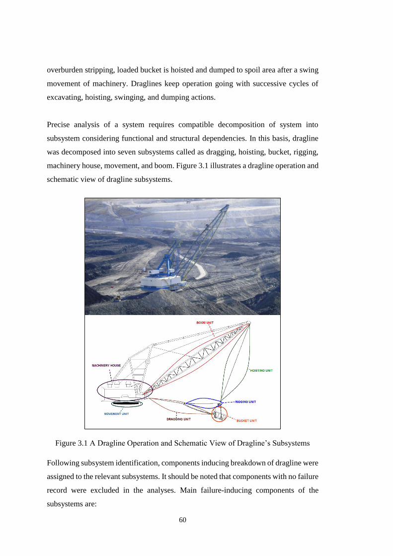
60

overburden stripping, loaded bucket is hoisted and dumped to spoil area after a swing

movement of machinery. Draglines keep operation going with successive cycles of

excavating, hoisting, swinging, and dumping actions.

Precise analysis of a system requires compatible decomposition of system into

subsystem considering functional and structural dependencies. In this basis, dragline

was decomposed into seven subsystems called as dragging, hoisting, bucket, rigging,

machinery house, movement, and boom. Figure 3.1 illustrates a dragline operation and

schematic view of dragline subsystems.

Figure 3.1 A Dragline Operation and Schematic View of Dragline’s Subsystems

Following subsystem identification, components inducing breakdown of dragline were

assigned to the relevant subsystems. It should be noted that components with no failure

record were excluded in the analyses. Main failure-inducing components of the

subsystems are:

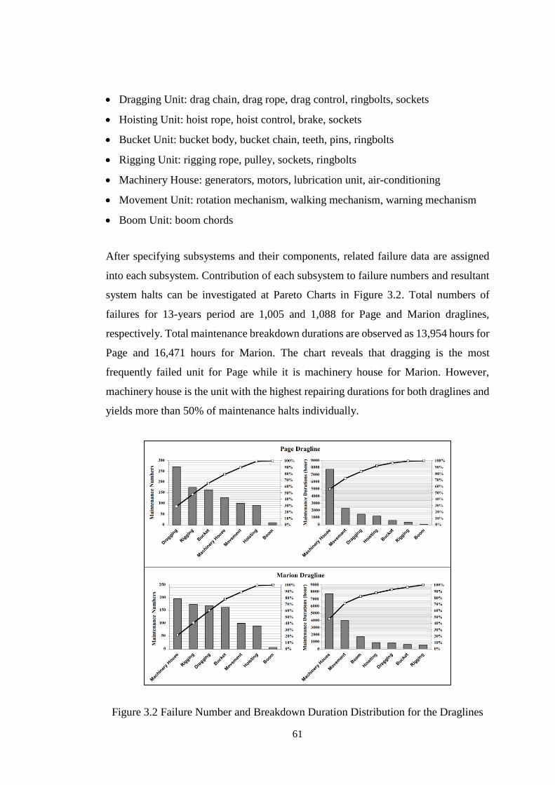
61

Dragging Unit: drag chain, drag rope, drag control, ringbolts, sockets

Hoisting Unit: hoist rope, hoist control, brake, sockets

Bucket Unit: bucket body, bucket chain, teeth, pins, ringbolts

Rigging Unit: rigging rope, pulley, sockets, ringbolts

Machinery House: generators, motors, lubrication unit, air-conditioning

Movement Unit: rotation mechanism, walking mechanism, warning mechanism

Boom Unit: boom chords

After specifying subsystems and their components, related failure data are assigned

into each subsystem. Contribution of each subsystem to failure numbers and resultant

system halts can be investigated at Pareto Charts in Figure 3.2. Total numbers of

failures for 13-years period are 1,005 and 1,088 for Page and Marion draglines,

respectively. Total maintenance breakdown durations are observed as 13,954 hours for

Page and 16,471 hours for Marion. The chart reveals that dragging is the most

frequently failed unit for Page while it is machinery house for Marion. However,

machinery house is the unit with the highest repairing durations for both draglines and

yields more than 50% of maintenance halts individually.

Figure 3.2 Failure Number and Breakdown Duration Distribution for the Draglines

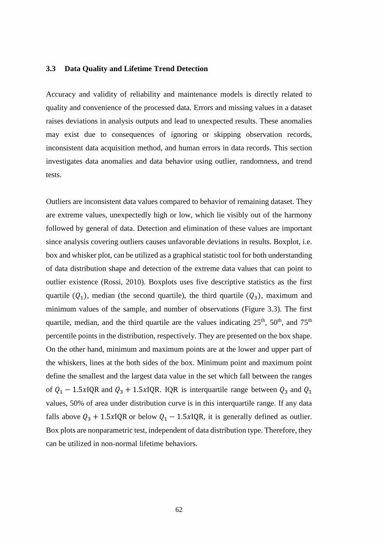
62

3.3 Data Quality and Lifetime Trend Detection

Accuracy and validity of reliability and maintenance models is directly related to

quality and convenience of the processed data. Errors and missing values in a dataset

raises deviations in analysis outputs and lead to unexpected results. These anomalies

may exist due to consequences of ignoring or skipping observation records,

inconsistent data acquisition method, and human errors in data records. This section

investigates data anomalies and data behavior using outlier, randomness, and trend

tests.

Outliers are inconsistent data values compared to behavior of remaining dataset. They

are extreme values, unexpectedly high or low, which lie visibly out of the harmony

followed by general of data. Detection and elimination of these values are important

since analysis covering outliers causes unfavorable deviations in results. Boxplot, i.e.

box and whisker plot, can be utilized as a graphical statistic tool for both understanding

of data distribution shape and detection of the extreme data values that can point to

outlier existence (Rossi, 2010). Boxplots uses five descriptive statistics as the first

quartile (𝑄1), median (the second quartile), the third quartile (𝑄3), maximum and

minimum values of the sample, and number of observations (Figure 3.3). The first

quartile, median, and the third quartile are the values indicating 25th, 50th, and 75th

percentile points in the distribution, respectively. They are presented on the box shape.

On the other hand, minimum and maximum points are at the lower and upper part of

the whiskers, lines at the both sides of the box. Minimum point and maximum point

define the smallest and the largest data value in the set which fall between the ranges

of 𝑄1 − 1.5𝑥IQR and 𝑄3 + 1.5𝑥IQR. IQR is interquartile range between 𝑄3 and 𝑄1

values, 50% of area under distribution curve is in this interquartile range. If any data

falls above 𝑄3 + 1.5𝑥IQR or below 𝑄1 − 1.5𝑥IQR, it is generally defined as outlier.

Box plots are nonparametric test, independent of data distribution type. Therefore, they

can be utilized in non-normal lifetime behaviors.

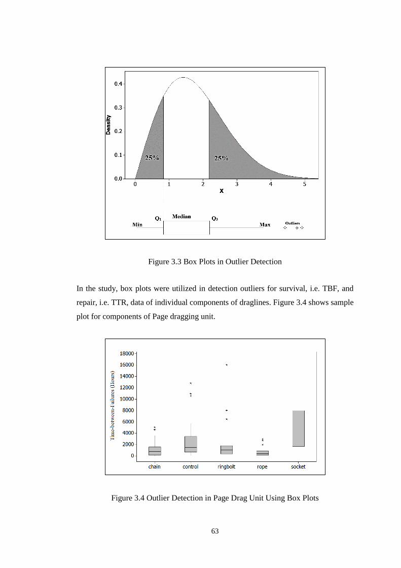
63

Figure 3.3 Box Plots in Outlier Detection

In the study, box plots were utilized in detection outliers for survival, i.e. TBF, and

repair, i.e. TTR, data of individual components of draglines. Figure 3.4 shows sample

plot for components of Page dragging unit.

Figure 3.4 Outlier Detection in Page Drag Unit Using Box Plots

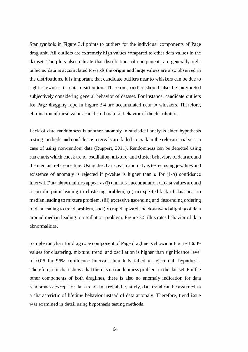
64

Star symbols in Figure 3.4 points to outliers for the individual components of Page

drag unit. All outliers are extremely high values compared to other data values in the

dataset. The plots also indicate that distributions of components are generally right

tailed so data is accumulated towards the origin and large values are also observed in

the distributions. It is important that candidate outliers near to whiskers can be due to

right skewness in data distribution. Therefore, outlier should also be interpreted

subjectively considering general behavior of dataset. For instance, candidate outliers

for Page dragging rope in Figure 3.4 are accumulated near to whiskers. Therefore,

elimination of these values can disturb natural behavior of the distribution.

Lack of data randomness is another anomaly in statistical analysis since hypothesis

testing methods and confidence intervals are failed to explain the relevant analysis in

case of using non-random data (Ruppert, 2011). Randomness can be detected using

run charts which check trend, oscillation, mixture, and cluster behaviors of data around

the median, reference line. Using the charts, each anomaly is tested using p-values and

existence of anomaly is rejected if p-value is higher than α for (1-α) confidence

interval. Data abnormalities appear as (i) unnatural accumulation of data values around

a specific point leading to clustering problem, (ii) unexpected lack of data near to

median leading to mixture problem, (iii) excessive ascending and descending ordering

of data leading to trend problem, and (iv) rapid upward and downward aligning of data

around median leading to oscillation problem. Figure 3.5 illustrates behavior of data

abnormalities.

Sample run chart for drag rope component of Page dragline is shown in Figure 3.6. P-

values for clustering, mixture, trend, and oscillation is higher than significance level

of 0.05 for 95% confidence interval, then it is failed to reject null hypothesis.

Therefore, run chart shows that there is no randomness problem in the dataset. For the

other components of both draglines, there is also no anomaly indication for data

randomness except for data trend. In a reliability study, data trend can be assumed as

a characteristic of lifetime behavior instead of data anomaly. Therefore, trend issue

was examined in detail using hypothesis testing methods.

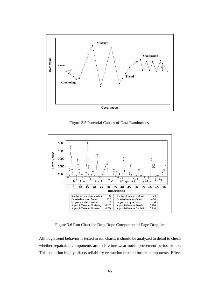
65

Figure 3.5 Potential Causes of Data Randomness

Figure 3.6 Run Chart for Drag Rope Component of Page Dragline

Although trend behavior is tested in run charts, it should be analyzed in detail to check

whether repairable components are in lifetime wear-out/improvement period or not.

This condition highly affects reliability evaluation method for the components. Effect

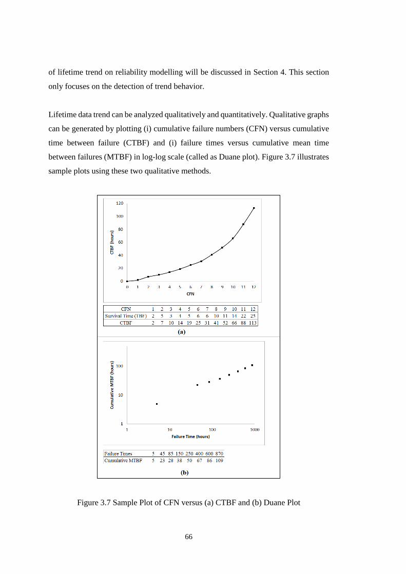
66

of lifetime trend on reliability modelling will be discussed in Section 4. This section

only focuses on the detection of trend behavior.

Lifetime data trend can be analyzed qualitatively and quantitatively. Qualitative graphs

can be generated by plotting (i) cumulative failure numbers (CFN) versus cumulative

time between failure (CTBF) and (i) failure times versus cumulative mean time

between failures (MTBF) in log-log scale (called as Duane plot). Figure 3.7 illustrates

sample plots using these two qualitative methods.

Figure 3.7 Sample Plot of CFN versus (a) CTBF and (b) Duane Plot

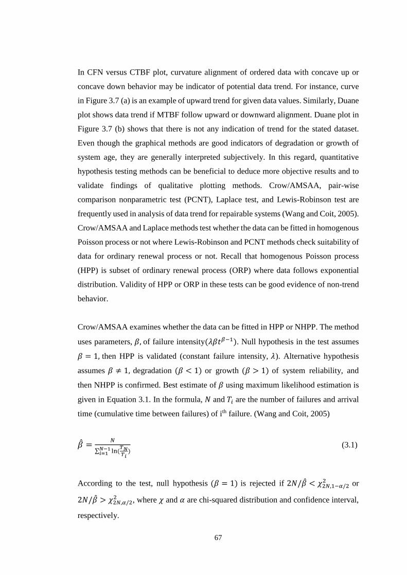
67

In CFN versus CTBF plot, curvature alignment of ordered data with concave up or

concave down behavior may be indicator of potential data trend. For instance, curve

in Figure 3.7 (a) is an example of upward trend for given data values. Similarly, Duane

plot shows data trend if MTBF follow upward or downward alignment. Duane plot in

Figure 3.7 (b) shows that there is not any indication of trend for the stated dataset.

Even though the graphical methods are good indicators of degradation or growth of

system age, they are generally interpreted subjectively. In this regard, quantitative

hypothesis testing methods can be beneficial to deduce more objective results and to

validate findings of qualitative plotting methods. Crow/AMSAA, pair-wise

comparison nonparametric test (PCNT), Laplace test, and Lewis-Robinson test are

frequently used in analysis of data trend for repairable systems (Wang and Coit, 2005).

Crow/AMSAA and Laplace methods test whether the data can be fitted in homogenous

Poisson process or not where Lewis-Robinson and PCNT methods check suitability of

data for ordinary renewal process or not. Recall that homogenous Poisson process

(HPP) is subset of ordinary renewal process (ORP) where data follows exponential

distribution. Validity of HPP or ORP in these tests can be good evidence of non-trend

behavior.

Crow/AMSAA examines whether the data can be fitted in HPP or NHPP. The method

uses parameters, 𝛽, of failure intensity(𝜆𝛽𝑡𝛽−1). Null hypothesis in the test assumes

𝛽 = 1, then HPP is validated (constant failure intensity, 𝜆). Alternative hypothesis

assumes 𝛽 ≠ 1, degradation (𝛽 < 1) or growth (𝛽 > 1) of system reliability, and

then NHPP is confirmed. Best estimate of 𝛽 using maximum likelihood estimation is

given in Equation 3.1. In the formula, 𝑁 and 𝑇𝑖 are the number of failures and arrival

time (cumulative time between failures) of ith failure. (Wang and Coit, 2005)

�̂� =𝑁

∑ ln (𝑇𝑁𝑇𝑖

)𝑁−1𝑖=1

(3.1)

According to the test, null hypothesis (𝛽 = 1) is rejected if 2𝑁/�̂� < 𝜒2𝑁,1−𝛼/22 or

2𝑁/�̂� > 𝜒2𝑁,𝛼/22 , where 𝜒 and 𝛼 are chi-squared distribution and confidence interval,

respectively.

68

Other trend test, PCNT, measures whether the data can be modelled using renewal

process or not. Presence of renewal process (null hypothesis) is rejected if 𝑈𝑝 > 𝑧𝛼/2

or 𝑈𝑝 < −𝑧𝛼/2 , 𝑈𝑝 can be evaluated using Equation 3.2. In the formula, N is the

number of failures and U is the number of cases where 𝑋𝑗 > 𝑋𝑖 for 𝑗 > 𝑖 (Wang and

Coit, 2005).

𝑈𝑝 =𝑈−𝑁(𝑁−1)/4

√(2𝑁+5)(𝑁−1)𝑁

72

(3.2)

The third trend test, Laplace test, investigates whether data is well fitted in HPP or

NHPP, as in Crow/AMSAA test. Acceptability of HPP (null hypothesis) is rejected if

𝑈𝐿 > 𝑧𝛼/2 or 𝑈𝐿 < −𝑧𝛼/2. Test statistics, 𝑈𝐿, is stated in Equation 3.3. In the formula,

𝑁 and 𝑇𝑖 are the number of failures and arrival time (cumulative time between failures)

of ith failure (Wang and Coit, 2005).

𝑈𝐿 =∑ 𝑇𝑖−(𝑁−1)

𝑇𝑁2

𝑁−1𝑖=1

𝑇𝑁√𝑁−1

12

(3.3)

The last trend test, Lewis-Robinson test, seeks whether data is fitted in renewal process

or not. Division of Laplace test statistics, 𝑈𝑝, to coefficient of variance is taken as

target test statistics as given in Equation 3.4. Coefficient of variance can be expressed

as √𝑉𝑎𝑟[𝑋]/�̅� where 𝑋 is TBF data. Again, null hypothesis rejected if 𝑈𝐿𝑅 > 𝑧𝛼/2 or

𝑈𝐿𝑅 < −𝑧𝛼/2 (Wang and Coit, 2005).

𝑈𝐿𝑅 =𝑈𝐿

𝐶𝑉[𝑋] (3.4)

Decisions of these tests can differ in some conditions where rejection value is in the

limits. Although Crow/AMSAA is highly robust test, decision about data trend can be

made considering results of the other tests, graphical illustration of lifetime trend, and

lifetime behavior in recent time. Test hypothesis of quantitative trend tests and their

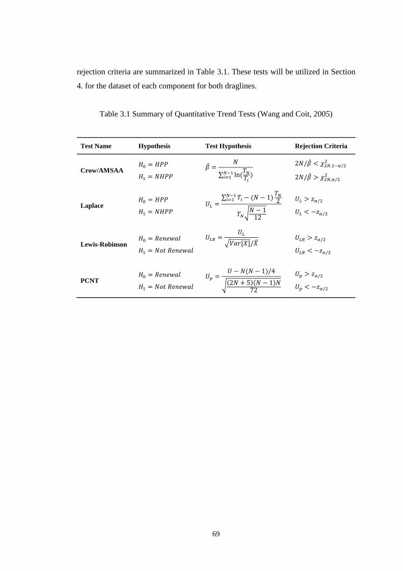
69

rejection criteria are summarized in Table 3.1. These tests will be utilized in Section

4. for the dataset of each component for both draglines.

Table 3.1 Summary of Quantitative Trend Tests (Wang and Coit, 2005)

Test Name Hypothesis Test Hypothesis Rejection Criteria

Crow/AMSAA 𝐻0 = 𝐻𝑃𝑃

𝐻1 = 𝑁𝐻𝑃𝑃

�̂� =𝑁

∑ ln (𝑇𝑁

𝑇𝑖)𝑁−1

𝑖=1

2𝑁/�̂� < 𝜒2𝑁,1−𝛼/2

2

2𝑁/�̂� > 𝜒2𝑁,𝛼/22

Laplace 𝐻0 = 𝐻𝑃𝑃

𝐻1 = 𝑁𝐻𝑃𝑃

𝑈𝐿 =∑ 𝑇𝑖 − (𝑁 − 1)

𝑇𝑁

2𝑁−1𝑖=1

𝑇𝑁√𝑁 − 112

𝑈𝐿 > 𝑧𝛼/2

𝑈𝐿 < −𝑧𝛼/2

Lewis-Robinson 𝐻0 = 𝑅𝑒𝑛𝑒𝑤𝑎𝑙

𝐻1 = 𝑁𝑜𝑡 𝑅𝑒𝑛𝑒𝑤𝑎𝑙

𝑈𝐿𝑅 =𝑈𝐿

√𝑉𝑎𝑟[𝑋]/�̅�

𝑈𝐿𝑅 > 𝑧𝛼/2

𝑈𝐿𝑅 < −𝑧𝛼/2

PCNT 𝐻0 = 𝑅𝑒𝑛𝑒𝑤𝑎𝑙

𝐻1 = 𝑁𝑜𝑡 𝑅𝑒𝑛𝑒𝑤𝑎𝑙

𝑈𝑝 =𝑈 − 𝑁(𝑁 − 1)/4

√(2𝑁 + 5)(𝑁 − 1)𝑁72

𝑈𝑝 > 𝑧𝛼/2

𝑈𝑝 < −𝑧𝛼/2

70

71

4. RELIABILITY OF WALKING DRAGLINES

4.1 Introduction

Energy demand in the global world and continual coal production in high quantities

have been a requirement to enhance dragline performance. Productivity of these

earthmovers is concerned by many interrelated components leaguing together to

generate the system. Estimation of component reliability is the main tool to forecast

the availability and reliability of the whole machinery. Deductive investigation

approach is generally utilized in reliability investigations to reveal the root-causes of

system failures. Components are the bottom elements of such a bottom-to-top

reliability investigation. Precise construction of functional dependencies between

components and subsystems is the primary issue to develop a system reliability model.

Dragline is a repairable system as other mining machineries. In the study, reliability

block diagrams (RBD) were utilized to describe top-to-bottom relationships in

subsystems and overall system. Reliability estimations of individual components were

achieved regarding their lifetime trends and repairability conditions. Component

repairability conditions were determined considering their maintenance type and

failure modes. On the other hand, lifetime wear-out or growth, i.e. trend, behavior of

components were detected via graphical and hypothesis testing methods as discussed

in Section 3.3. Repairable component with lifetime trend were processed using general

renewal process (GRP). Reliability of stationary repairable components and non-

repairable component were estimated via best-fit distributions. In addition to reliability

estimation, general renewal process was also utilized to examine maintenance

effectiveness on dragline subsystems. Methodology to be utilized in this section can

be viewed from Figure 4.1

72

STARTS

Specify subsystems

Allocate components

to subsystems

Distribute

failure data to

components

Eliminate outliers

Start reliability estimation

for components

TREND TESTS for

COMPONENT FAILURE

DATA

Qualitative Trend Test

Graph of Cumulative Survival

Times

Quantitative Trend Tests

Crow/AMSAA

Pair-Wise Comparison

Nonparametric Test

Laplace Test

Lewis-Robinson Test

Is there lifetime trend?

Use general renewal

process for component

Is failure number 30?

Best-fit distribution using

maximum likelihood

estimation (MLE)

Best-fit distribution using

rank regression on X

(RRX)

Is component repairable?

Construction of

dependencies between

components

Subsystem reliability

estimation

Dragline reliability

estimation

Distribute failure data to

subsystems

Use general renewal

process for subsystems

Estimate shape and scale

parameters

Find system restoration

factors

Evaluate reliability

and maintenance

values

END

No

Yes

No

Yes

No

Yes

System Reliability Estimation Maintenance Effectiveness Estimation

Figure 4.1 Methodology of the System Reliability Analysis

73

4.2 Reliabilities of Draglines’ Subsystems

This section covers reliability and maintenance effectiveness estimations for

individual subsystems of draglines. In the study, reliability modelling of draglines

were achieved via reliability block diagrams and regarded both component reliabilities

and their functional effects on the systems. Dragline is a combination of subsystems

called as dragging, hoisting, bucket, rigging, machinery house, movement, and boom.

Subsystem components are configured in a particular design to ensure different

functionalities of dragline. Lifetime performance of each component has different

effect on subsystem according to their functional and structural features.

Reliability estimation methods of components are affected from their repairability and

lifetime trend behaviors (Figure 4.1). Repairability conditions can be investigated

considering failure modes and resultant maintenance types where lifetime trend can be

discussed using hypothesis tests and graphical lifetime illustrations. If a component is

always replaced with an identical one in case of failure, it is called as non-repairable

component. Corrective repairing for these components are generally not practical and

economic. Since there is no any lifetime aging/growth behavior for non-repairable

components, reliability of them can be estimated using best-fit distributions of time-

to-failure values. On the other hand, a component is called as repairable if replacement

of it after all failures is structurally and economically impossible. If component is

detected to be repairable, then lifetime trend behavior should be examined.

Components without any non-stationary deterioration or growth in their lifetimes are

called as non-trend components. In this case, it is understood that the component is

almost maintained to as good as new condition and they behave like non-repairable

components. Therefore, best-fit distributions of time between failures values can be

utilized for these components. If there is increasing/decreasing lifetime trend,

reliability of these non-stationary components can be estimated using general renewal

process (GRP). It should be noted that a repairable component can cover non-

repairable sub-components. Therefore, repairability condition can change according to

the definition boundary of components. Repairability assumptions of dragline

components can be viewed in Table 4.1. Lifetime trend behavior of the components

will be discussed in Sections 4.2.1-4.2.7.

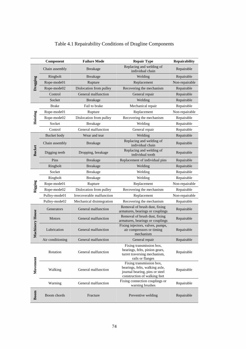
74

Table 4.1 Repairability Conditions of Dragline Components

Component Failure Mode Repair Type Repairability

Dra

gg

ing

Chain assembly Breakage Replacing and welding of

individual chain Repairable

Ringbolt Breakage Welding Repairable

Rope-mode01 Rupture Replacement Non-repairable

Rope-mode02 Dislocation from pulley Recovering the mechanism Repairable

Control General malfunction General repair Repairable

Socket Breakage Welding Repairable

Ho

isti

ng

Brake Fail to brake Mechanical repair Repairable

Rope-mode01 Rupture Replacement Non-repairable

Rope-mode02 Dislocation from pulley Recovering the mechanism Repairable

Socket Breakage Welding Repairable

Control General malfunction General repair Repairable

Bu

cket

Bucket body Wear and tear Welding Repairable

Chain assembly Breakage Replacing and welding of

individual chain Repairable

Digging teeth Dropping, breakage Replacing and welding of

individual tooth Repairable

Pins Breakage Replacement of individual pins Repairable

Ringbolt Breakage Welding Repairable

Rig

gin

g

Socket Breakage Welding Repairable

Ringbolt Breakage Welding Repairable

Rope-mode01 Rupture Replacement Non-repairable

Rope-mode02 Dislocation from pulley Recovering the mechanism Repairable

Pulley-mode01 Irrecoverable malfunction Replacement Non-repairable

Pulley-mode02 Mechanical disintegration Recovering the mechanism Repairable

Ma

chin

ery

Hou

se Generators General malfunction

Removal of brush dust, fixing

armatures, bearings or couplings Repairable

Motors General malfunction Removal of brush dust, fixing

armatures, bearings or couplings Repairable

Lubrication General malfunction Fixing injectors, valves, pumps,

air compressors or timing

mechanism

Repairable

Air conditioning General malfunction General repair Repairable

Mo

vem

ent

Rotation General malfunction

Fixing transmission box,

bearings, felts, pinion gears,

turret traversing mechanism,

rails or flanges

Repairable

Walking General malfunction

Fixing transmission box,

bearings, felts, walking axle,

journal bearing, pins or steel

construction of walking feet

Repairable

Warning General malfunction Fixing connection couplings or

warning brushes Repairable

Bo

om

Boom chords Fracture Preventive welding Repairable

75

As seen in Table 4.1, rope components of dragging, hoisting and rigging units are non-

repairable components. However, these components may exhibit two different failure

modes as rupture and dislocation from mechanism. If rupture exists, rope is replaced

with a new one. On the other hand, dislocation from mechanism is recovered with

repairing activity without component replacement. Rupture mode in the study were

called as rope-mode1 to specify its non-repairable condition. Moreover, components

such as, chain, pin, digging tooth are generally maintained with sub-component

replacement. They were assumed as repairable sets including non-repairable

individual components. For instance, pin component is repairable set which covers

individual non-repairable pins.

4.2.1 Dragging Unit

Overburden stripping is achieved through dragging of dragline bucket. Dragging unit

comprises individual components utilized for pull-back action of bucket toward

machinery house in order to fill the bucket with loose ground material. Dragging chain,

dragging rope, control elements, socket, and ringbolt are the main components of this

unit. Reliability of dragging unit were evaluated via reliability estimation of these

components. Then, effect of maintenance to subsystem recovery was discussed using

general renewal process.

As stated in Figure 4.1, repairability condition and existence of lifetime trend effect

reliability assessment method. In this sense, drag rope-mode01 is only non-repairable

component in dragging units (Table 4.1). For repairable components, lifetime trend

behaviors were analyzed using graphical trend tests (Figures 4.2-4.3) and hypothesis

tests in 90% confidence interval (Tables 4.2-4.3). Trend tests indicated that chain

assembly and rope-mode2 are the candidate components for lifetime trend in Marion

dragging unit. Rope-mode2 slightly yields alternative hypothesis for PCNT and Lewis

Robinson tests. Figure 4.2 also supports that this component is at the beginning of

trend behavior. Therefore, it was assumed non-trend component. Eventually, chain

assembly is only trend component in Marion dragging system. Reliability of it was

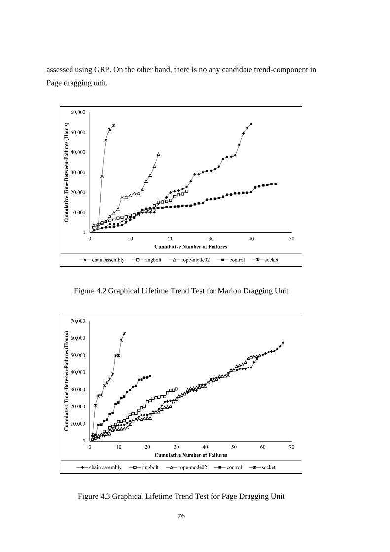
76

assessed using GRP. On the other hand, there is no any candidate trend-component in

Page dragging unit.

Figure 4.2 Graphical Lifetime Trend Test for Marion Dragging Unit

Figure 4.3 Graphical Lifetime Trend Test for Page Dragging Unit

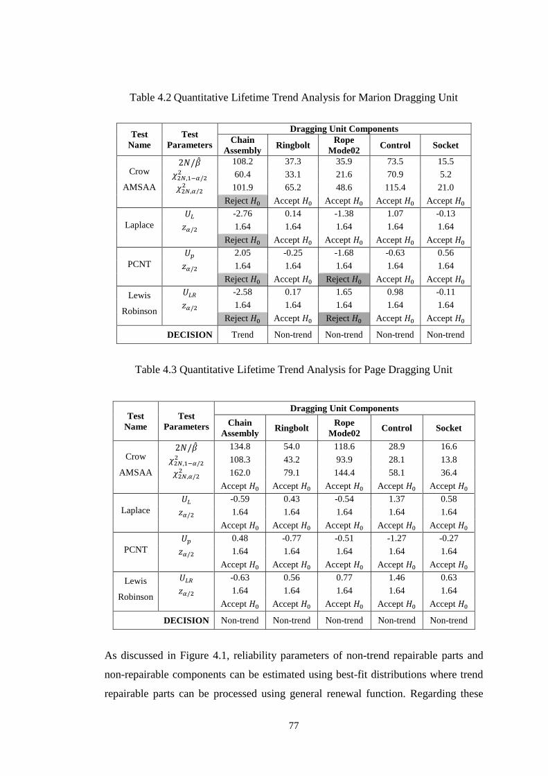
77

Table 4.2 Quantitative Lifetime Trend Analysis for Marion Dragging Unit

Test

Name

Test

Parameters

Dragging Unit Components

Chain

Assembly Ringbolt

Rope

Mode02 Control Socket

Crow

AMSAA

2𝑁/�̂� 108.2 37.3 35.9 73.5 15.5

𝜒2𝑁,1−𝛼/22 60.4 33.1 21.6 70.9 5.2

𝜒2𝑁,𝛼/22 101.9 65.2 48.6 115.4 21.0

Reject 𝐻0 Accept 𝐻0 Accept 𝐻0 Accept 𝐻0 Accept 𝐻0

Laplace

𝑈𝐿 -2.76 0.14 -1.38 1.07 -0.13

𝑧𝛼/2 1.64 1.64 1.64 1.64 1.64

Reject 𝐻0 Accept 𝐻0 Accept 𝐻0 Accept 𝐻0 Accept 𝐻0

PCNT

𝑈𝑝 2.05 -0.25 -1.68 -0.63 0.56

𝑧𝛼/2 1.64 1.64 1.64 1.64 1.64

Reject 𝐻0 Accept 𝐻0 Reject 𝐻0 Accept 𝐻0 Accept 𝐻0

Lewis

Robinson

𝑈𝐿𝑅 -2.58 0.17 1.65 0.98 -0.11

𝑧𝛼/2 1.64 1.64 1.64 1.64 1.64

Reject 𝐻0 Accept 𝐻0 Reject 𝐻0 Accept 𝐻0 Accept 𝐻0

DECISION Trend Non-trend Non-trend Non-trend Non-trend

Table 4.3 Quantitative Lifetime Trend Analysis for Page Dragging Unit

Test

Name

Test

Parameters

Dragging Unit Components

Chain

Assembly Ringbolt

Rope

Mode02 Control Socket

Crow

AMSAA

2𝑁/�̂� 134.8 54.0 118.6 28.9 16.6

𝜒2𝑁,1−𝛼/22 108.3 43.2 93.9 28.1 13.8

𝜒2𝑁,𝛼/22 162.0 79.1 144.4 58.1 36.4

Accept 𝐻0 Accept 𝐻0 Accept 𝐻0 Accept 𝐻0 Accept 𝐻0

Laplace

𝑈𝐿 -0.59 0.43 -0.54 1.37 0.58

𝑧𝛼/2 1.64 1.64 1.64 1.64 1.64

Accept 𝐻0 Accept 𝐻0 Accept 𝐻0 Accept 𝐻0 Accept 𝐻0

PCNT

𝑈𝑝 0.48 -0.77 -0.51 -1.27 -0.27

𝑧𝛼/2 1.64 1.64 1.64 1.64 1.64

Accept 𝐻0 Accept 𝐻0 Accept 𝐻0 Accept 𝐻0 Accept 𝐻0

Lewis

Robinson

𝑈𝐿𝑅 -0.63 0.56 0.77 1.46 0.63

𝑧𝛼/2 1.64 1.64 1.64 1.64 1.64

Accept 𝐻0 Accept 𝐻0 Accept 𝐻0 Accept 𝐻0 Accept 𝐻0

DECISION Non-trend Non-trend Non-trend Non-trend Non-trend

As discussed in Figure 4.1, reliability parameters of non-trend repairable parts and

non-repairable components can be estimated using best-fit distributions where trend

repairable parts can be processed using general renewal function. Regarding these

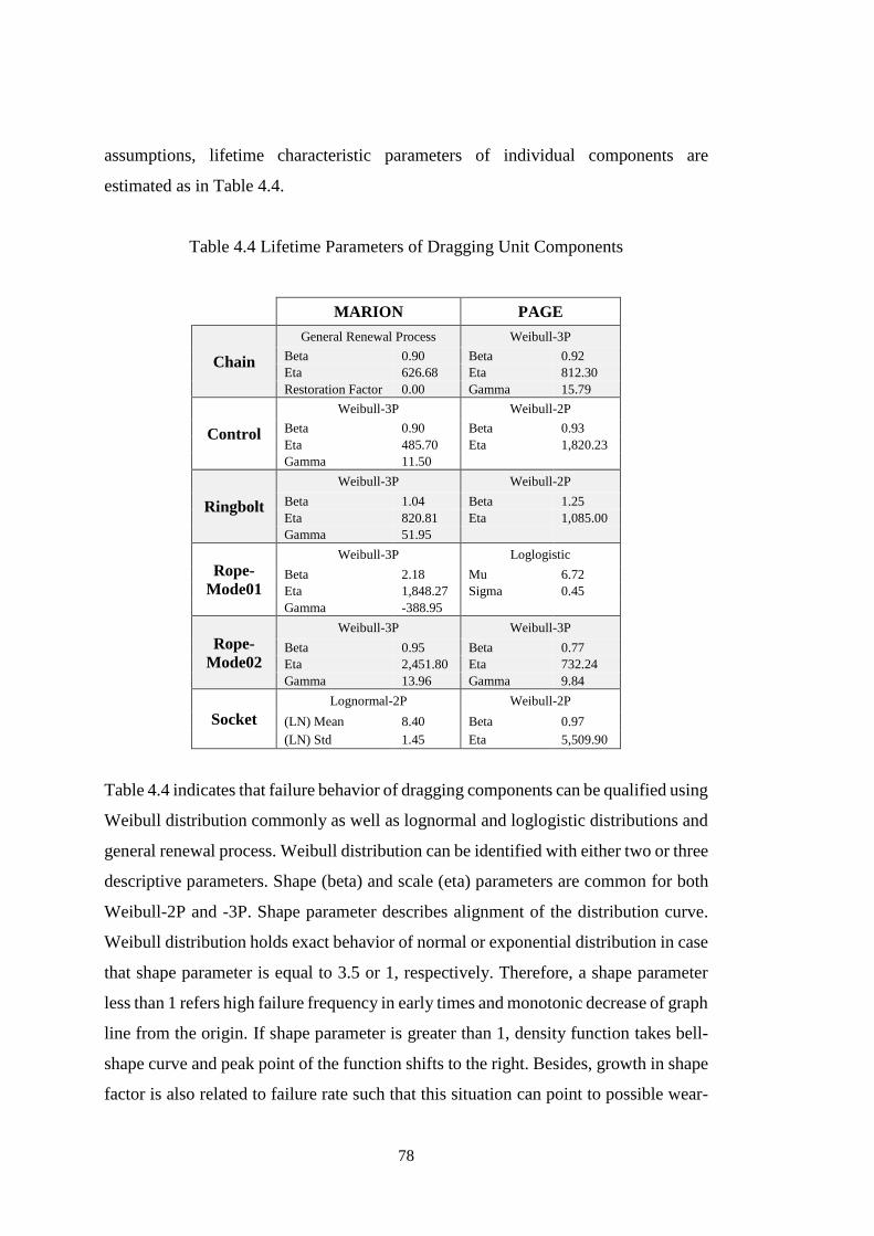
78

assumptions, lifetime characteristic parameters of individual components are

estimated as in Table 4.4.

Table 4.4 Lifetime Parameters of Dragging Unit Components

MARION PAGE

Chain

General Renewal Process Weibull-3P

Beta 0.90 Beta 0.92

Eta 626.68 Eta 812.30

Restoration Factor 0.00 Gamma 15.79

Control

Weibull-3P Weibull-2P

Beta 0.90 Beta 0.93

Eta 485.70 Eta 1,820.23

Gamma 11.50

Ringbolt

Weibull-3P Weibull-2P

Beta 1.04 Beta 1.25

Eta 820.81 Eta 1,085.00

Gamma 51.95

Rope-

Mode01

Weibull-3P Loglogistic

Beta 2.18 Mu 6.72

Eta 1,848.27 Sigma 0.45

Gamma -388.95

Rope-

Mode02

Weibull-3P Weibull-3P

Beta 0.95 Beta 0.77

Eta 2,451.80 Eta 732.24

Gamma 13.96 Gamma 9.84

Socket

Lognormal-2P Weibull-2P

(LN) Mean 8.40 Beta 0.97

(LN) Std 1.45 Eta 5,509.90

Table 4.4 indicates that failure behavior of dragging components can be qualified using

Weibull distribution commonly as well as lognormal and loglogistic distributions and

general renewal process. Weibull distribution can be identified with either two or three

descriptive parameters. Shape (beta) and scale (eta) parameters are common for both

Weibull-2P and -3P. Shape parameter describes alignment of the distribution curve.

Weibull distribution holds exact behavior of normal or exponential distribution in case

that shape parameter is equal to 3.5 or 1, respectively. Therefore, a shape parameter

less than 1 refers high failure frequency in early times and monotonic decrease of graph

line from the origin. If shape parameter is greater than 1, density function takes bell-

shape curve and peak point of the function shifts to the right. Besides, growth in shape

factor is also related to failure rate such that this situation can point to possible wear-

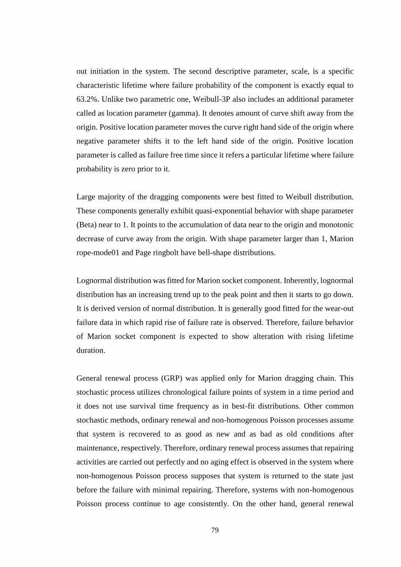
79

out initiation in the system. The second descriptive parameter, scale, is a specific

characteristic lifetime where failure probability of the component is exactly equal to

63.2%. Unlike two parametric one, Weibull-3P also includes an additional parameter

called as location parameter (gamma). It denotes amount of curve shift away from the

origin. Positive location parameter moves the curve right hand side of the origin where

negative parameter shifts it to the left hand side of the origin. Positive location

parameter is called as failure free time since it refers a particular lifetime where failure

probability is zero prior to it.

Large majority of the dragging components were best fitted to Weibull distribution.

These components generally exhibit quasi-exponential behavior with shape parameter

(Beta) near to 1. It points to the accumulation of data near to the origin and monotonic

decrease of curve away from the origin. With shape parameter larger than 1, Marion

rope-mode01 and Page ringbolt have bell-shape distributions.

Lognormal distribution was fitted for Marion socket component. Inherently, lognormal

distribution has an increasing trend up to the peak point and then it starts to go down.

It is derived version of normal distribution. It is generally good fitted for the wear-out

failure data in which rapid rise of failure rate is observed. Therefore, failure behavior

of Marion socket component is expected to show alteration with rising lifetime

duration.

General renewal process (GRP) was applied only for Marion dragging chain. This

stochastic process utilizes chronological failure points of system in a time period and

it does not use survival time frequency as in best-fit distributions. Other common

stochastic methods, ordinary renewal and non-homogenous Poisson processes assume

that system is recovered to as good as new and as bad as old conditions after

maintenance, respectively. Therefore, ordinary renewal process assumes that repairing

activities are carried out perfectly and no aging effect is observed in the system where

non-homogenous Poisson process supposes that system is returned to the state just

before the failure with minimal repairing. Therefore, systems with non-homogenous

Poisson process continue to age consistently. On the other hand, general renewal

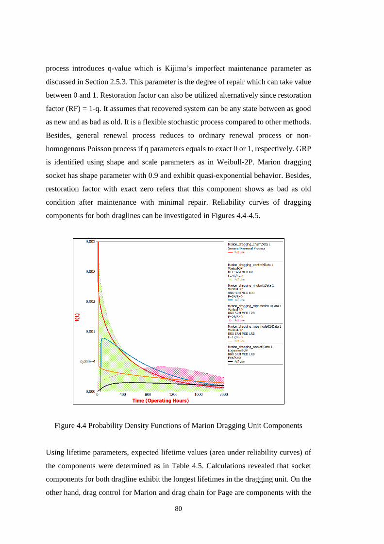
80

process introduces q-value which is Kijima’s imperfect maintenance parameter as

discussed in Section 2.5.3. This parameter is the degree of repair which can take value

between 0 and 1. Restoration factor can also be utilized alternatively since restoration

factor (RF) = 1-q. It assumes that recovered system can be any state between as good

as new and as bad as old. It is a flexible stochastic process compared to other methods.

Besides, general renewal process reduces to ordinary renewal process or non-

homogenous Poisson process if q parameters equals to exact 0 or 1, respectively. GRP

is identified using shape and scale parameters as in Weibull-2P. Marion dragging

socket has shape parameter with 0.9 and exhibit quasi-exponential behavior. Besides,

restoration factor with exact zero refers that this component shows as bad as old

condition after maintenance with minimal repair. Reliability curves of dragging

components for both draglines can be investigated in Figures 4.4-4.5.

Figure 4.4 Probability Density Functions of Marion Dragging Unit Components

Using lifetime parameters, expected lifetime values (area under reliability curves) of

the components were determined as in Table 4.5. Calculations revealed that socket

components for both dragline exhibit the longest lifetimes in the dragging unit. On the

other hand, drag control for Marion and drag chain for Page are components with the

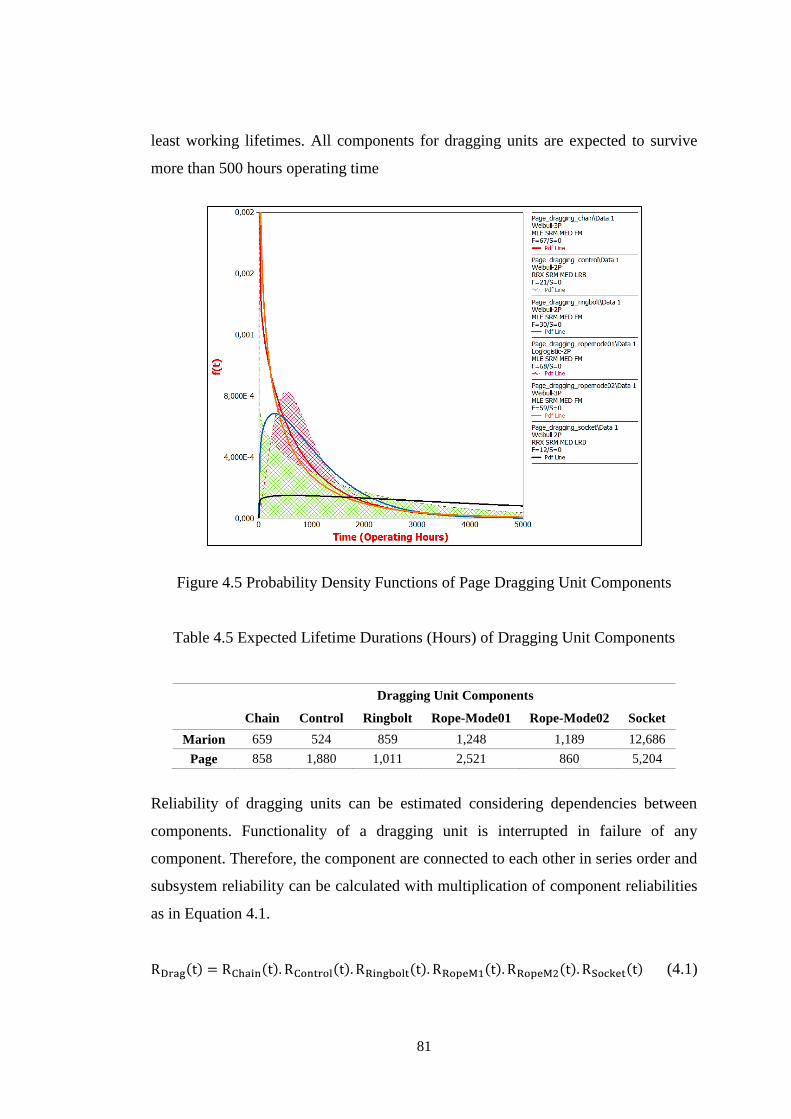
81

least working lifetimes. All components for dragging units are expected to survive

more than 500 hours operating time

Figure 4.5 Probability Density Functions of Page Dragging Unit Components

Table 4.5 Expected Lifetime Durations (Hours) of Dragging Unit Components

Dragging Unit Components

Chain Control Ringbolt Rope-Mode01 Rope-Mode02 Socket

Marion 659 524 859 1,248 1,189 12,686

Page 858 1,880 1,011 2,521 860 5,204

Reliability of dragging units can be estimated considering dependencies between

components. Functionality of a dragging unit is interrupted in failure of any

component. Therefore, the component are connected to each other in series order and

subsystem reliability can be calculated with multiplication of component reliabilities

as in Equation 4.1.

RDrag(t) = RChain(t). RControl(t). RRingbolt(t). RRopeM1(t). RRopeM2(t). RSocket(t) (4.1)

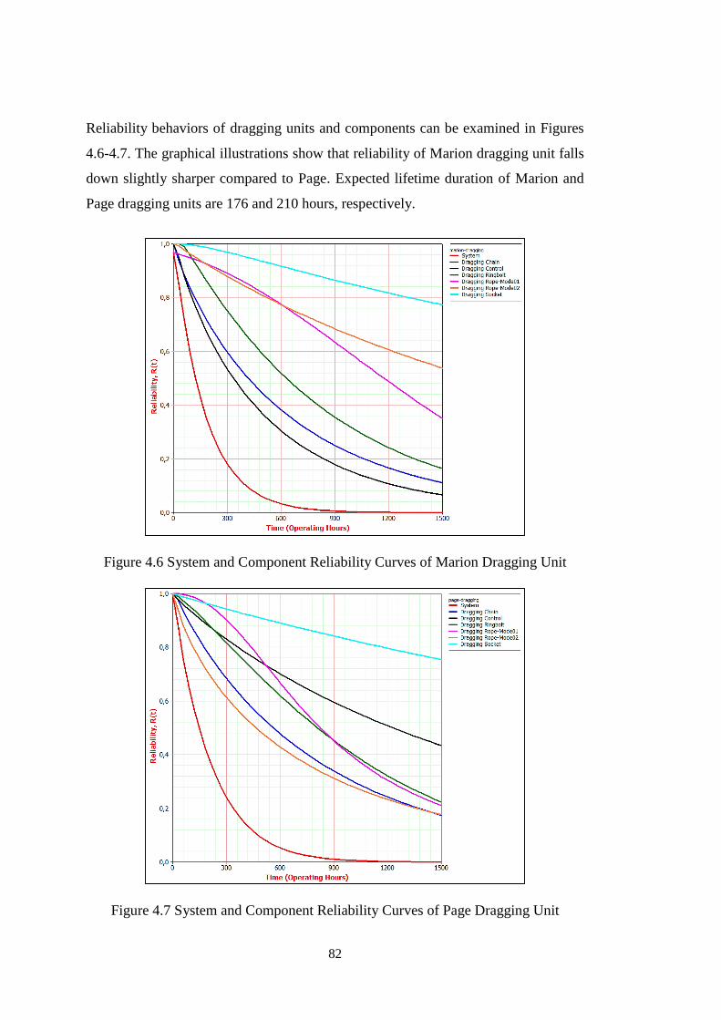
82

Reliability behaviors of dragging units and components can be examined in Figures

4.6-4.7. The graphical illustrations show that reliability of Marion dragging unit falls

down slightly sharper compared to Page. Expected lifetime duration of Marion and

Page dragging units are 176 and 210 hours, respectively.

Figure 4.6 System and Component Reliability Curves of Marion Dragging Unit

Figure 4.7 System and Component Reliability Curves of Page Dragging Unit

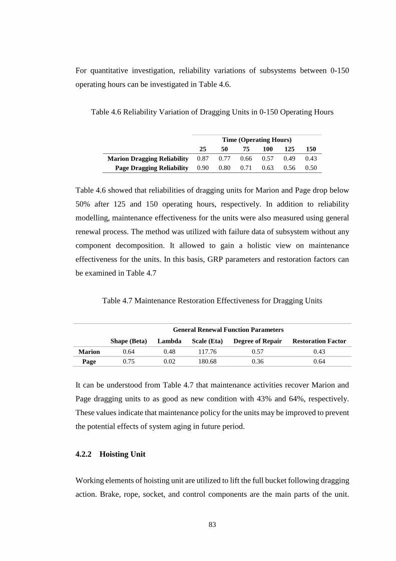
83

For quantitative investigation, reliability variations of subsystems between 0-150

operating hours can be investigated in Table 4.6.

Table 4.6 Reliability Variation of Dragging Units in 0-150 Operating Hours

Time (Operating Hours)

25 50 75 100 125 150

Marion Dragging Reliability 0.87 0.77 0.66 0.57 0.49 0.43

Page Dragging Reliability 0.90 0.80 0.71 0.63 0.56 0.50

Table 4.6 showed that reliabilities of dragging units for Marion and Page drop below

50% after 125 and 150 operating hours, respectively. In addition to reliability

modelling, maintenance effectiveness for the units were also measured using general

renewal process. The method was utilized with failure data of subsystem without any

component decomposition. It allowed to gain a holistic view on maintenance

effectiveness for the units. In this basis, GRP parameters and restoration factors can

be examined in Table 4.7

Table 4.7 Maintenance Restoration Effectiveness for Dragging Units

General Renewal Function Parameters

Shape (Beta) Lambda Scale (Eta) Degree of Repair Restoration Factor

Marion 0.64 0.48 117.76 0.57 0.43

Page 0.75 0.02 180.68 0.36 0.64

It can be understood from Table 4.7 that maintenance activities recover Marion and

Page dragging units to as good as new condition with 43% and 64%, respectively.

These values indicate that maintenance policy for the units may be improved to prevent

the potential effects of system aging in future period.

4.2.2 Hoisting Unit

Working elements of hoisting unit are utilized to lift the full bucket following dragging

action. Brake, rope, socket, and control components are the main parts of the unit.

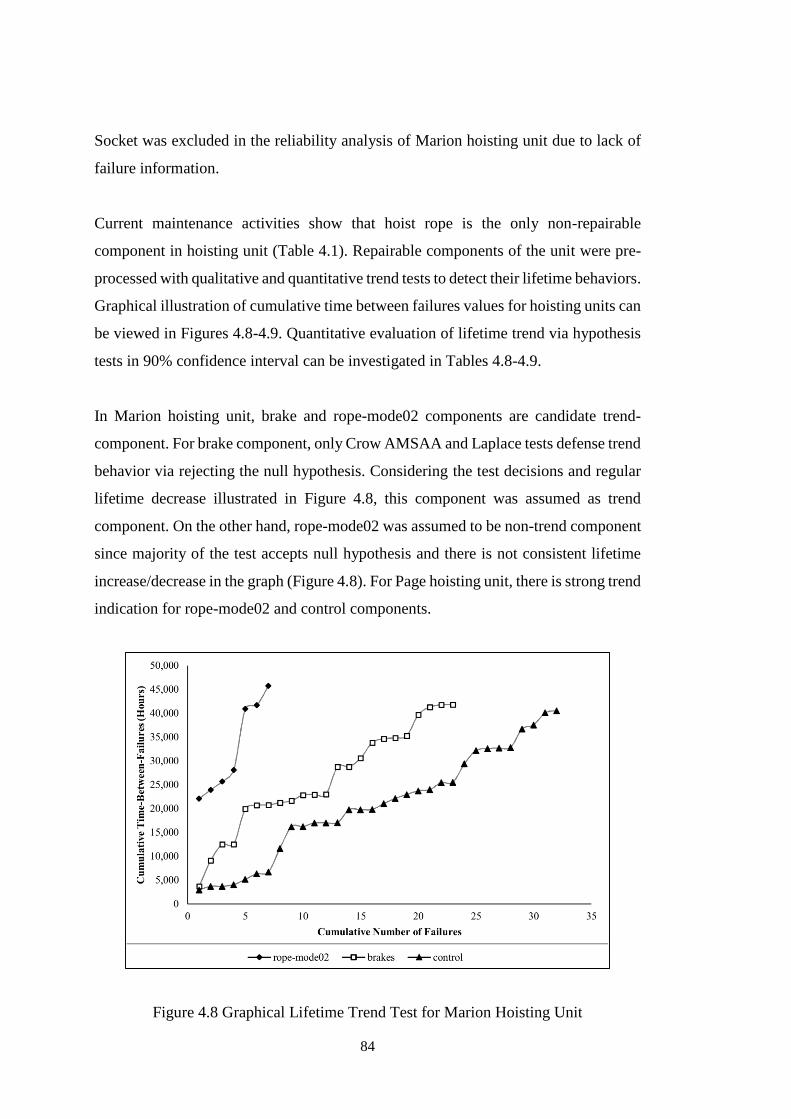
84

Socket was excluded in the reliability analysis of Marion hoisting unit due to lack of

failure information.

Current maintenance activities show that hoist rope is the only non-repairable

component in hoisting unit (Table 4.1). Repairable components of the unit were pre-

processed with qualitative and quantitative trend tests to detect their lifetime behaviors.

Graphical illustration of cumulative time between failures values for hoisting units can

be viewed in Figures 4.8-4.9. Quantitative evaluation of lifetime trend via hypothesis

tests in 90% confidence interval can be investigated in Tables 4.8-4.9.

In Marion hoisting unit, brake and rope-mode02 components are candidate trend-

component. For brake component, only Crow AMSAA and Laplace tests defense trend

behavior via rejecting the null hypothesis. Considering the test decisions and regular

lifetime decrease illustrated in Figure 4.8, this component was assumed as trend

component. On the other hand, rope-mode02 was assumed to be non-trend component

since majority of the test accepts null hypothesis and there is not consistent lifetime

increase/decrease in the graph (Figure 4.8). For Page hoisting unit, there is strong trend

indication for rope-mode02 and control components.

Figure 4.8 Graphical Lifetime Trend Test for Marion Hoisting Unit

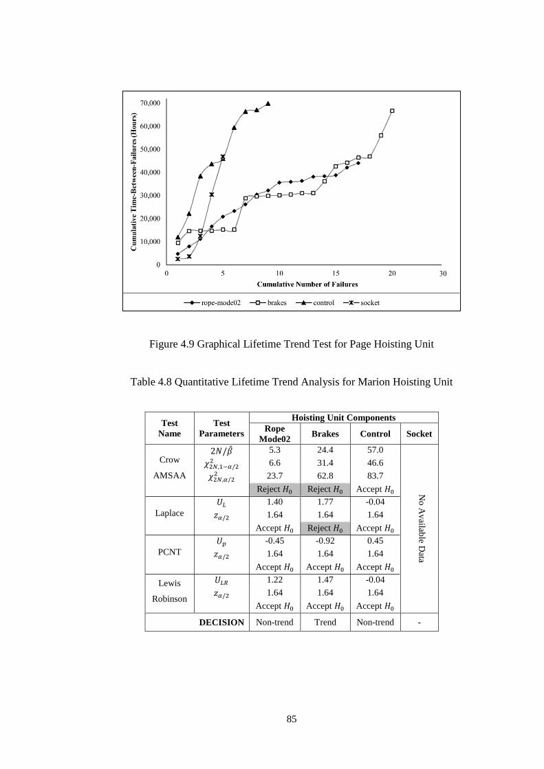
85

Figure 4.9 Graphical Lifetime Trend Test for Page Hoisting Unit

Table 4.8 Quantitative Lifetime Trend Analysis for Marion Hoisting Unit

Test

Name

Test

Parameters

Hoisting Unit Components

Rope

Mode02 Brakes Control Socket

Crow

AMSAA

2𝑁/�̂� 5.3 24.4 57.0

No

Av

ailable D

ata

𝜒2𝑁,1−𝛼/22 6.6 31.4 46.6

𝜒2𝑁,𝛼/22 23.7 62.8 83.7

Reject 𝐻0 Reject 𝐻0 Accept 𝐻0

Laplace

𝑈𝐿 1.40 1.77 -0.04

𝑧𝛼/2 1.64 1.64 1.64

Accept 𝐻0 Reject 𝐻0 Accept 𝐻0

PCNT

𝑈𝑝 -0.45 -0.92 0.45

𝑧𝛼/2 1.64 1.64 1.64

Accept 𝐻0 Accept 𝐻0 Accept 𝐻0

Lewis

Robinson

𝑈𝐿𝑅 1.22 1.47 -0.04

𝑧𝛼/2 1.64 1.64 1.64

Accept 𝐻0 Accept 𝐻0 Accept 𝐻0

DECISION Non-trend Trend Non-trend -

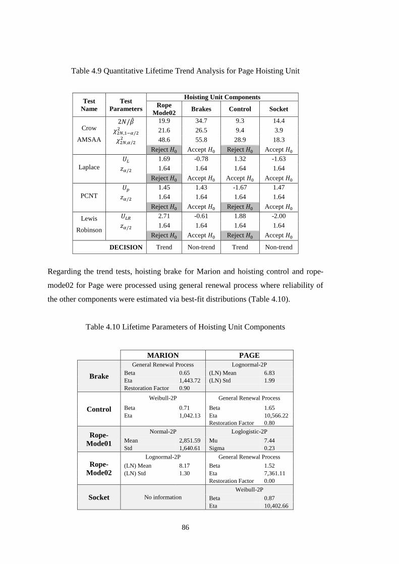
86

Table 4.9 Quantitative Lifetime Trend Analysis for Page Hoisting Unit

Test

Name

Test

Parameters

Hoisting Unit Components

Rope

Mode02 Brakes Control Socket

Crow

AMSAA

2𝑁/�̂� 19.9 34.7 9.3 14.4

𝜒2𝑁,1−𝛼/22 21.6 26.5 9.4 3.9

𝜒2𝑁,𝛼/22 48.6 55.8 28.9 18.3

Reject 𝐻0 Accept 𝐻0 Reject 𝐻0 Accept 𝐻0

Laplace

𝑈𝐿 1.69 -0.78 1.32 -1.63

𝑧𝛼/2 1.64 1.64 1.64 1.64

Reject 𝐻0 Accept 𝐻0 Accept 𝐻0 Accept 𝐻0

PCNT

𝑈𝑝 1.45 1.43 -1.67 1.47

𝑧𝛼/2 1.64 1.64 1.64 1.64

Reject 𝐻0 Accept 𝐻0 Reject 𝐻0 Accept 𝐻0

Lewis

Robinson

𝑈𝐿𝑅 2.71 -0.61 1.88 -2.00

𝑧𝛼/2 1.64 1.64 1.64 1.64

Reject 𝐻0 Accept 𝐻0 Reject 𝐻0 Accept 𝐻0

DECISION Trend Non-trend Trend Non-trend

Regarding the trend tests, hoisting brake for Marion and hoisting control and rope-

mode02 for Page were processed using general renewal process where reliability of

the other components were estimated via best-fit distributions (Table 4.10).

Table 4.10 Lifetime Parameters of Hoisting Unit Components

MARION PAGE

Brake

General Renewal Process Lognormal-2P

Beta 0.65 (LN) Mean 6.83

Eta 1,443.72 (LN) Std 1.99

Restoration Factor 0.90

Control

Weibull-2P General Renewal Process

Beta 0.71 Beta 1.65

Eta 1,042.13 Eta 10,566.22

Restoration Factor 0.80

Rope-

Mode01

Normal-2P Loglogistic-2P

Mean 2,851.59 Mu 7.44

Std 1,640.61 Sigma 0.23

Rope-

Mode02

Lognormal-2P General Renewal Process

(LN) Mean 8.17 Beta 1.52

(LN) Std 1.30 Eta 7,361.11

Restoration Factor 0.00

Socket No information

Weibull-2P

Beta 0.87

Eta 10,402.66

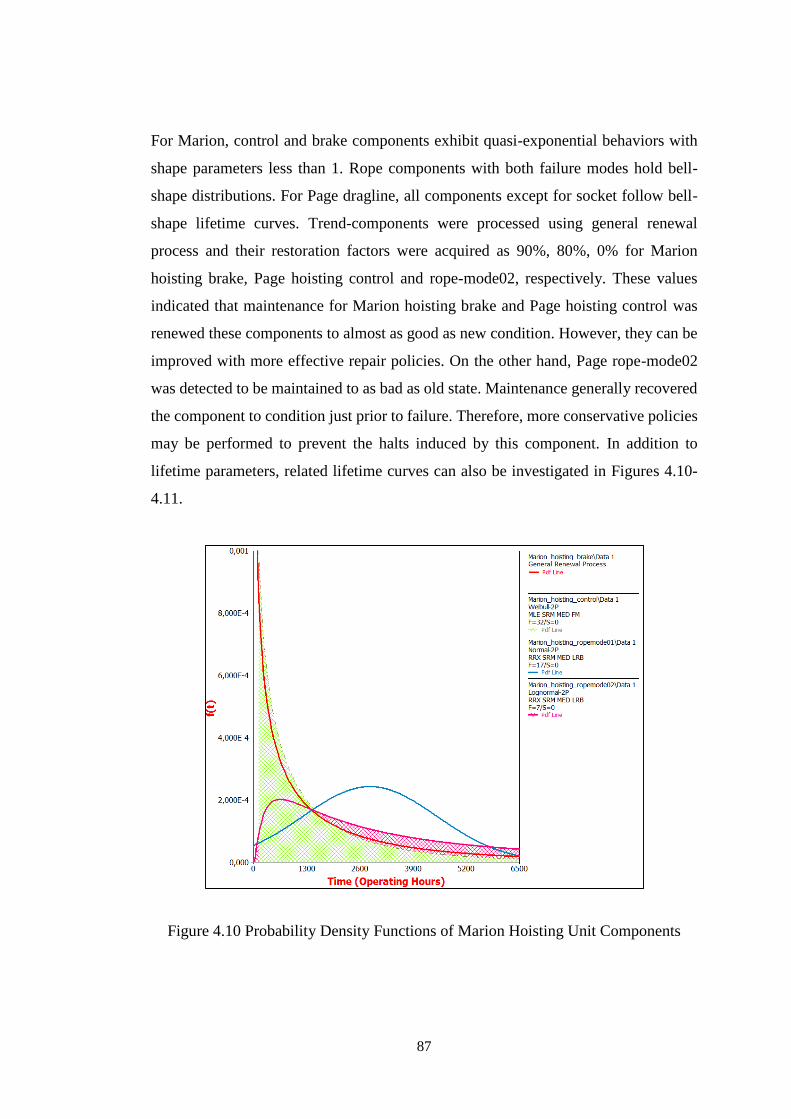
87

For Marion, control and brake components exhibit quasi-exponential behaviors with

shape parameters less than 1. Rope components with both failure modes hold bell-

shape distributions. For Page dragline, all components except for socket follow bell-

shape lifetime curves. Trend-components were processed using general renewal

process and their restoration factors were acquired as 90%, 80%, 0% for Marion

hoisting brake, Page hoisting control and rope-mode02, respectively. These values

indicated that maintenance for Marion hoisting brake and Page hoisting control was

renewed these components to almost as good as new condition. However, they can be

improved with more effective repair policies. On the other hand, Page rope-mode02

was detected to be maintained to as bad as old state. Maintenance generally recovered

the component to condition just prior to failure. Therefore, more conservative policies

may be performed to prevent the halts induced by this component. In addition to

lifetime parameters, related lifetime curves can also be investigated in Figures 4.10-

4.11.

Figure 4.10 Probability Density Functions of Marion Hoisting Unit Components

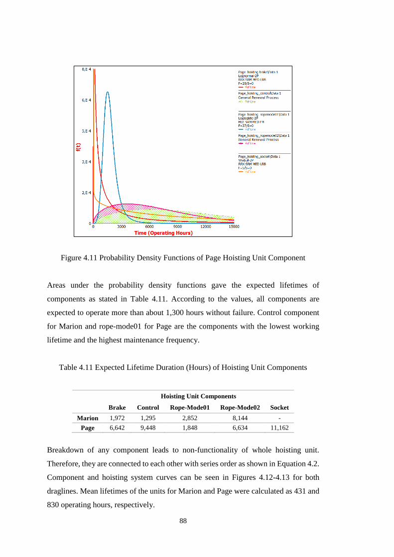
88

Figure 4.11 Probability Density Functions of Page Hoisting Unit Component

Areas under the probability density functions gave the expected lifetimes of

components as stated in Table 4.11. According to the values, all components are

expected to operate more than about 1,300 hours without failure. Control component

for Marion and rope-mode01 for Page are the components with the lowest working

lifetime and the highest maintenance frequency.

Table 4.11 Expected Lifetime Duration (Hours) of Hoisting Unit Components

Hoisting Unit Components

Brake Control Rope-Mode01 Rope-Mode02 Socket

Marion 1,972 1,295 2,852 8,144 -

Page 6,642 9,448 1,848 6,634 11,162

Breakdown of any component leads to non-functionality of whole hoisting unit.

Therefore, they are connected to each other with series order as shown in Equation 4.2.

Component and hoisting system curves can be seen in Figures 4.12-4.13 for both

draglines. Mean lifetimes of the units for Marion and Page were calculated as 431 and

830 operating hours, respectively.

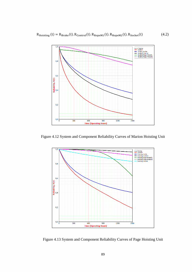
89

RHoisting (t) = RBrake(t). RControl(t). RRopeM1(t). RRopeM2(t). RSocket(t) (4.2)

Figure 4.12 System and Component Reliability Curves of Marion Hoisting Unit

Figure 4.13 System and Component Reliability Curves of Page Hoisting Unit

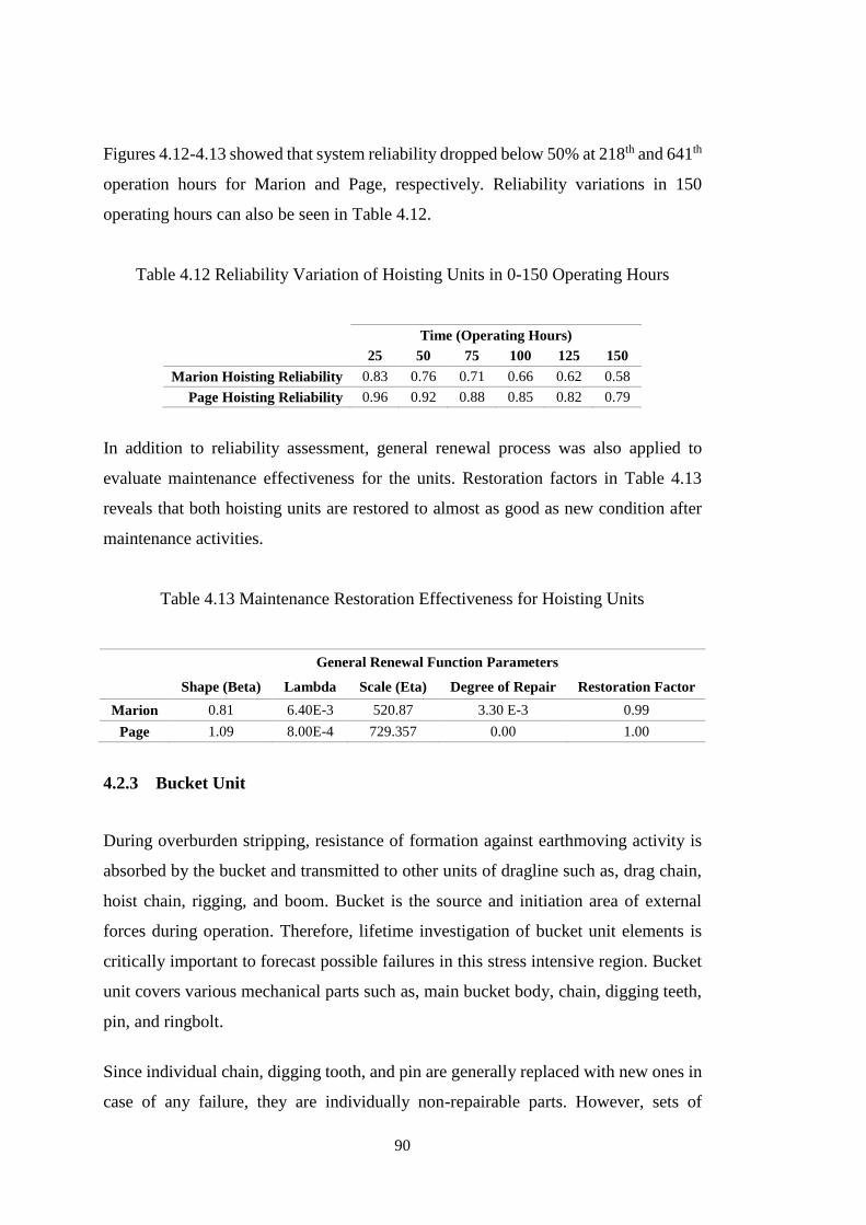
90

Figures 4.12-4.13 showed that system reliability dropped below 50% at 218th and 641th

operation hours for Marion and Page, respectively. Reliability variations in 150

operating hours can also be seen in Table 4.12.

Table 4.12 Reliability Variation of Hoisting Units in 0-150 Operating Hours

Time (Operating Hours)

25 50 75 100 125 150

Marion Hoisting Reliability 0.83 0.76 0.71 0.66 0.62 0.58

Page Hoisting Reliability 0.96 0.92 0.88 0.85 0.82 0.79

In addition to reliability assessment, general renewal process was also applied to

evaluate maintenance effectiveness for the units. Restoration factors in Table 4.13

reveals that both hoisting units are restored to almost as good as new condition after

maintenance activities.

Table 4.13 Maintenance Restoration Effectiveness for Hoisting Units

General Renewal Function Parameters

Shape (Beta) Lambda Scale (Eta) Degree of Repair Restoration Factor

Marion 0.81 6.40E-3 520.87 3.30 E-3 0.99

Page 1.09 8.00E-4 729.357 0.00 1.00

4.2.3 Bucket Unit

During overburden stripping, resistance of formation against earthmoving activity is

absorbed by the bucket and transmitted to other units of dragline such as, drag chain,

hoist chain, rigging, and boom. Bucket is the source and initiation area of external

forces during operation. Therefore, lifetime investigation of bucket unit elements is

critically important to forecast possible failures in this stress intensive region. Bucket

unit covers various mechanical parts such as, main bucket body, chain, digging teeth,

pin, and ringbolt.

Since individual chain, digging tooth, and pin are generally replaced with new ones in

case of any failure, they are individually non-repairable parts. However, sets of

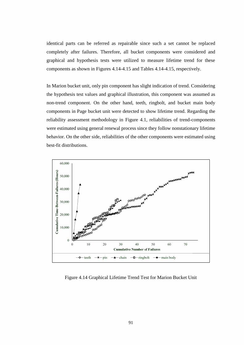
91

identical parts can be referred as repairable since such a set cannot be replaced

completely after failures. Therefore, all bucket components were considered and

graphical and hypothesis tests were utilized to measure lifetime trend for these

components as shown in Figures 4.14-4.15 and Tables 4.14-4.15, respectively.

In Marion bucket unit, only pin component has slight indication of trend. Considering

the hypothesis test values and graphical illustration, this component was assumed as

non-trend component. On the other hand, teeth, ringbolt, and bucket main body

components in Page bucket unit were detected to show lifetime trend. Regarding the

reliability assessment methodology in Figure 4.1, reliabilities of trend-components

were estimated using general renewal process since they follow nonstationary lifetime

behavior. On the other side, reliabilities of the other components were estimated using

best-fit distributions.

Figure 4.14 Graphical Lifetime Trend Test for Marion Bucket Unit

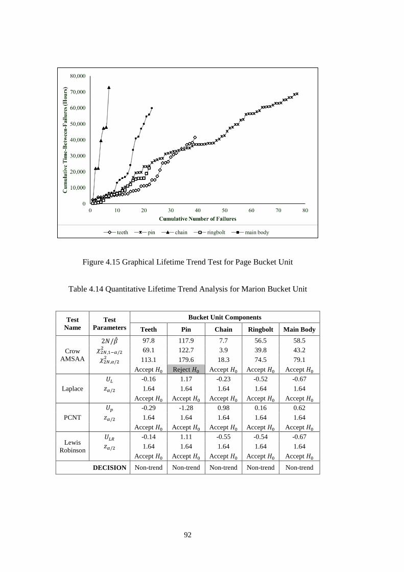
92

Figure 4.15 Graphical Lifetime Trend Test for Page Bucket Unit

Table 4.14 Quantitative Lifetime Trend Analysis for Marion Bucket Unit

Test

Name

Test

Parameters

Bucket Unit Components

Teeth Pin Chain Ringbolt Main Body

Crow

AMSAA

2𝑁/�̂� 97.8 117.9 7.7 56.5 58.5

𝜒2𝑁,1−𝛼/22 69.1 122.7 3.9 39.8 43.2

𝜒2𝑁,𝛼/22 113.1 179.6 18.3 74.5 79.1

Accept 𝐻0 Reject 𝐻0 Accept 𝐻0 Accept 𝐻0 Accept 𝐻0

Laplace

𝑈𝐿 -0.16 1.17 -0.23 -0.52 -0.67

𝑧𝛼/2 1.64 1.64 1.64 1.64 1.64

Accept 𝐻0 Accept 𝐻0 Accept 𝐻0 Accept 𝐻0 Accept 𝐻0

PCNT

𝑈𝑝 -0.29 -1.28 0.98 0.16 0.62

𝑧𝛼/2 1.64 1.64 1.64 1.64 1.64

Accept 𝐻0 Accept 𝐻0 Accept 𝐻0 Accept 𝐻0 Accept 𝐻0

Lewis

Robinson

𝑈𝐿𝑅 -0.14 1.11 -0.55 -0.54 -0.67

𝑧𝛼/2 1.64 1.64 1.64 1.64 1.64

Accept 𝐻0 Accept 𝐻0 Accept 𝐻0 Accept 𝐻0 Accept 𝐻0

DECISION Non-trend Non-trend Non-trend Non-trend Non-trend

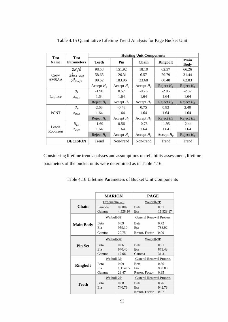
93

Table 4.15 Quantitative Lifetime Trend Analysis for Page Bucket Unit

Test

Name

Test

Parameters

Hoisting Unit Components

Teeth Pin Chain Ringbolt Main

Body

Crow

AMSAA

2𝑁/�̂� 98.58 151.92 18.10 62.57 66.26

𝜒2𝑁,1−𝛼/22 58.65 126.31 6.57 29.79 31.44

𝜒2𝑁,𝛼/22 99.62 183.96 23.68 60.48 62.83

Accept 𝐻0 Accept 𝐻0 Accept 𝐻0 Reject 𝐻0 Reject 𝐻0

Laplace

𝑈𝐿 -1.90 0.57 -0.76 -2.05 -2.32

𝑧𝛼/2 1.64 1.64 1.64 1.64 1.64

Reject 𝐻0 Accept 𝐻0 Accept 𝐻0 Reject 𝐻0 Reject 𝐻0

PCNT

𝑈𝑝 2.63 -0.48 0.75 0.82 2.40

𝑧𝛼/2 1.64 1.64 1.64 1.64 1.64

Reject 𝐻0 Accept 𝐻0 Accept 𝐻0 Reject 𝐻0 Reject 𝐻0

Lewis

Robinson

𝑈𝐿𝑅 -1.69 0.56 -0.73 -1.95 -2.44

𝑧𝛼/2 1.64 1.64 1.64 1.64 1.64

Reject 𝐻0 Accept 𝐻0 Accept 𝐻0 Accept 𝐻0 Reject 𝐻0

DECISION Trend Non-trend Non-trend Trend Trend

Considering lifetime trend analyses and assumptions on reliability assessment, lifetime

parameters of the bucket units were determined as in Table 4.16.

Table 4.16 Lifetime Parameters of Bucket Unit Components

MARION PAGE

Chain Exponential-2P Weibull-2P

Lambda 0,0002 Beta 0.61

Gamma 4,528.10 Eta 11,528.17

Main Body

Weibull-3P General Renewal Process

Beta 0.89 Beta 0.72

Eta 959.10 Eta 788.92

Gamma 20.75 Restor. Factor 0.00

Pin Set

Weibull-3P Weibull-3P

Beta 0.86 Beta 0.91

Eta 640.40 Eta 873.43

Gamma 12.66 Gamma 31.31

Ringbolt

Weibull-3P General Renewal Process

Beta 0.99 Beta 0.86

Eta 1,114.85 Eta 988.83

Gamma 28.47 Restor. Factor 0.85

Teeth

Weibull-2P General Renewal Process

Beta 0.88 Beta 0.76

Eta 740.79 Eta 942.78

Restor. Factor 0.97

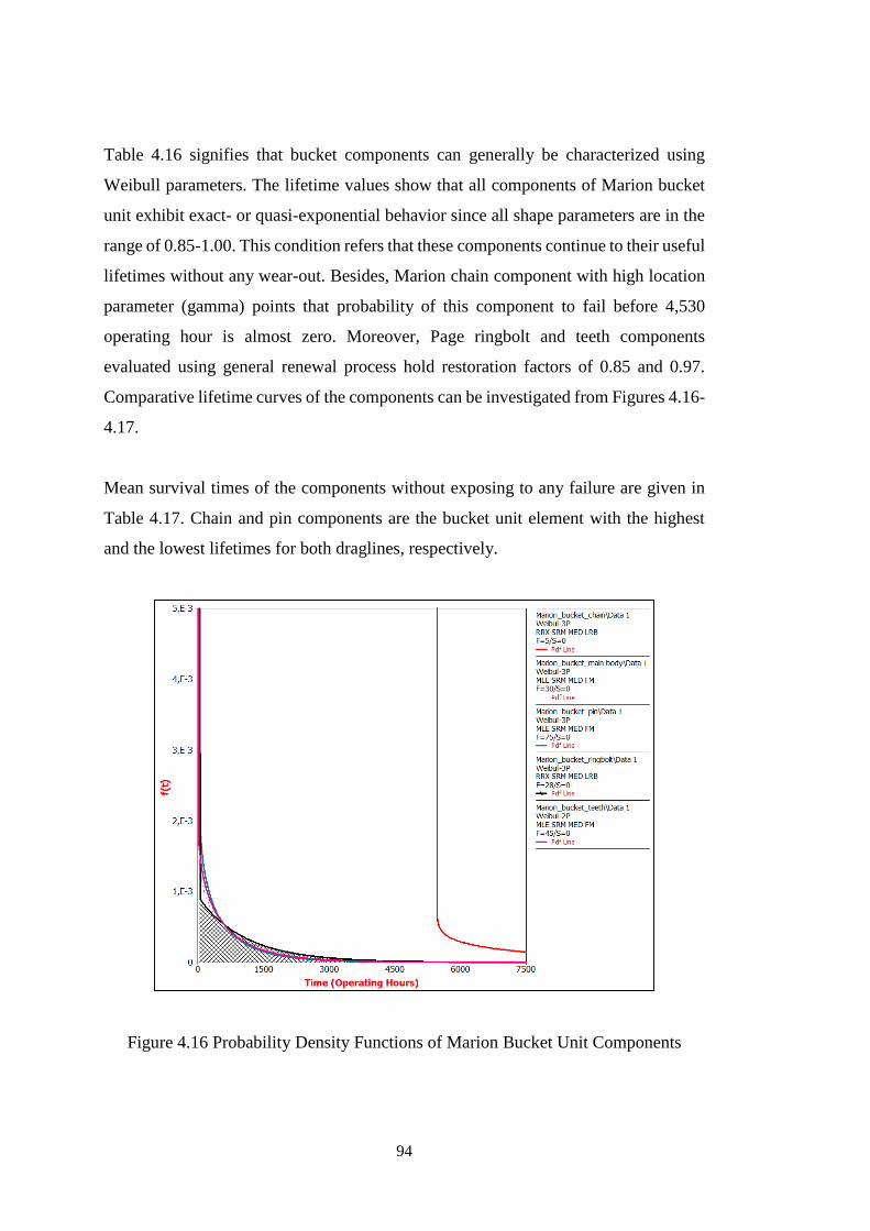
94

Table 4.16 signifies that bucket components can generally be characterized using

Weibull parameters. The lifetime values show that all components of Marion bucket

unit exhibit exact- or quasi-exponential behavior since all shape parameters are in the

range of 0.85-1.00. This condition refers that these components continue to their useful

lifetimes without any wear-out. Besides, Marion chain component with high location

parameter (gamma) points that probability of this component to fail before 4,530

operating hour is almost zero. Moreover, Page ringbolt and teeth components

evaluated using general renewal process hold restoration factors of 0.85 and 0.97.

Comparative lifetime curves of the components can be investigated from Figures 4.16-

4.17.

Mean survival times of the components without exposing to any failure are given in

Table 4.17. Chain and pin components are the bucket unit element with the highest

and the lowest lifetimes for both draglines, respectively.

Figure 4.16 Probability Density Functions of Marion Bucket Unit Components

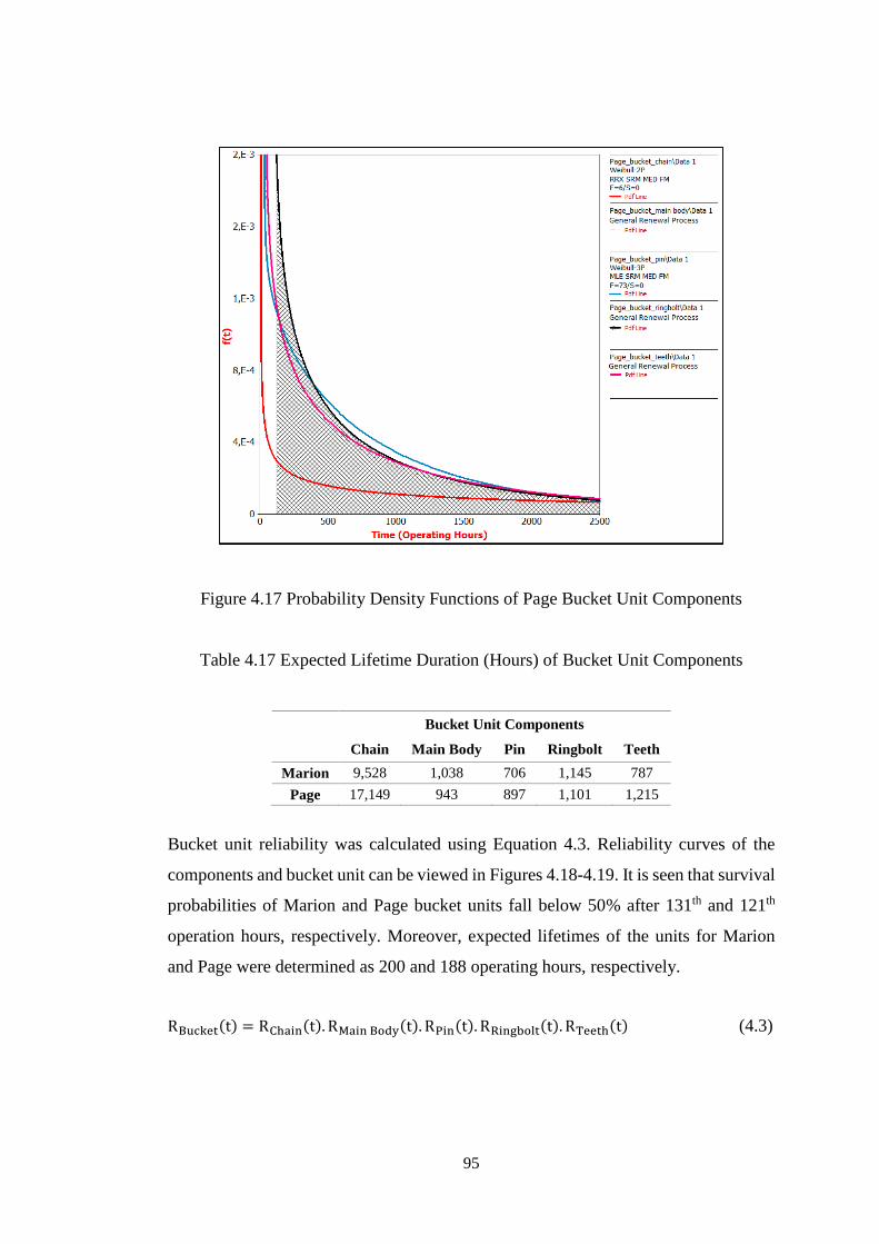
95

Figure 4.17 Probability Density Functions of Page Bucket Unit Components

Table 4.17 Expected Lifetime Duration (Hours) of Bucket Unit Components

Bucket Unit Components

Chain Main Body Pin Ringbolt Teeth

Marion 9,528 1,038 706 1,145 787

Page 17,149 943 897 1,101 1,215

Bucket unit reliability was calculated using Equation 4.3. Reliability curves of the

components and bucket unit can be viewed in Figures 4.18-4.19. It is seen that survival

probabilities of Marion and Page bucket units fall below 50% after 131th and 121th

operation hours, respectively. Moreover, expected lifetimes of the units for Marion

and Page were determined as 200 and 188 operating hours, respectively.

RBucket(t) = RChain(t). RMain Body(t). RPin(t). RRingbolt(t). RTeeth(t) (4.3)

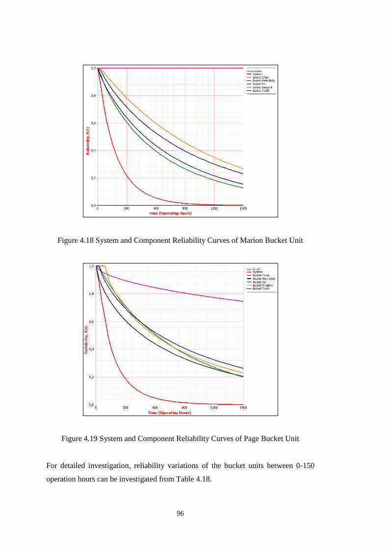
96

Figure 4.18 System and Component Reliability Curves of Marion Bucket Unit

Figure 4.19 System and Component Reliability Curves of Page Bucket Unit

For detailed investigation, reliability variations of the bucket units between 0-150

operation hours can be investigated from Table 4.18.

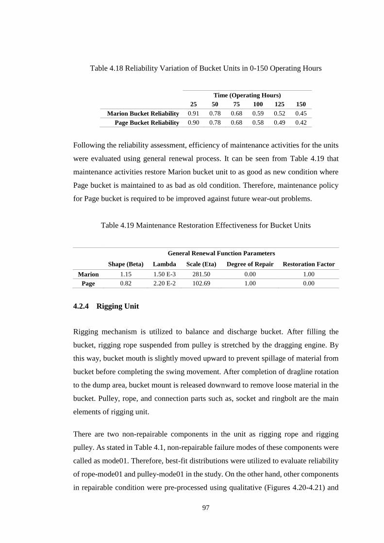
97

Table 4.18 Reliability Variation of Bucket Units in 0-150 Operating Hours

Time (Operating Hours)

25 50 75 100 125 150

Marion Bucket Reliability 0.91 0.78 0.68 0.59 0.52 0.45

Page Bucket Reliability 0.90 0.78 0.68 0.58 0.49 0.42

Following the reliability assessment, efficiency of maintenance activities for the units

were evaluated using general renewal process. It can be seen from Table 4.19 that

maintenance activities restore Marion bucket unit to as good as new condition where

Page bucket is maintained to as bad as old condition. Therefore, maintenance policy

for Page bucket is required to be improved against future wear-out problems.

Table 4.19 Maintenance Restoration Effectiveness for Bucket Units

General Renewal Function Parameters

Shape (Beta) Lambda Scale (Eta) Degree of Repair Restoration Factor

Marion 1.15 1.50 E-3 281.50 0.00 1.00

Page 0.82 2.20 E-2 102.69 1.00 0.00

4.2.4 Rigging Unit

Rigging mechanism is utilized to balance and discharge bucket. After filling the

bucket, rigging rope suspended from pulley is stretched by the dragging engine. By

this way, bucket mouth is slightly moved upward to prevent spillage of material from

bucket before completing the swing movement. After completion of dragline rotation

to the dump area, bucket mount is released downward to remove loose material in the

bucket. Pulley, rope, and connection parts such as, socket and ringbolt are the main

elements of rigging unit.

There are two non-repairable components in the unit as rigging rope and rigging

pulley. As stated in Table 4.1, non-repairable failure modes of these components were

called as mode01. Therefore, best-fit distributions were utilized to evaluate reliability

of rope-mode01 and pulley-mode01 in the study. On the other hand, other components

in repairable condition were pre-processed using qualitative (Figures 4.20-4.21) and

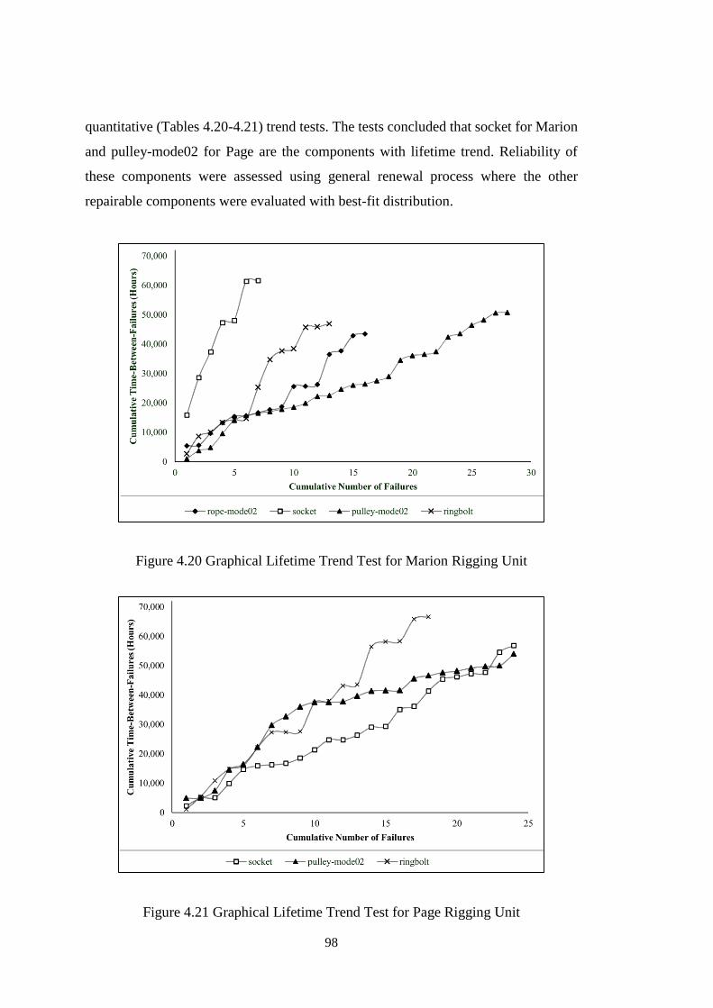
98

quantitative (Tables 4.20-4.21) trend tests. The tests concluded that socket for Marion

and pulley-mode02 for Page are the components with lifetime trend. Reliability of

these components were assessed using general renewal process where the other

repairable components were evaluated with best-fit distribution.

Figure 4.20 Graphical Lifetime Trend Test for Marion Rigging Unit

Figure 4.21 Graphical Lifetime Trend Test for Page Rigging Unit

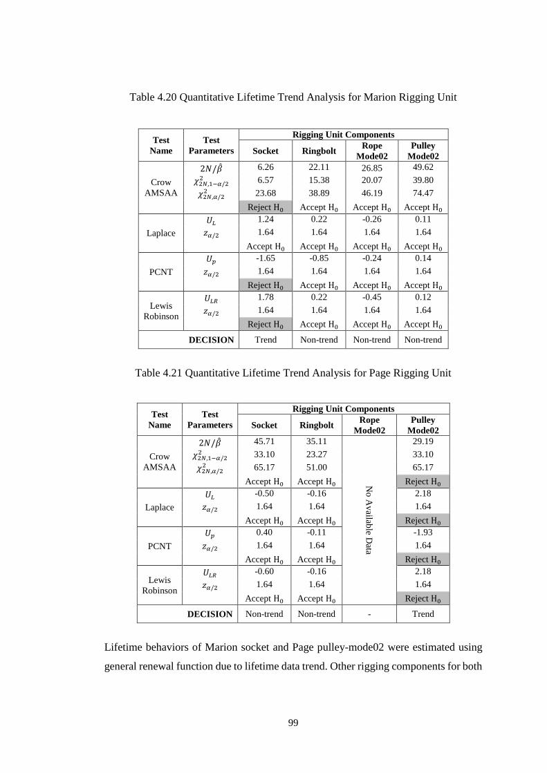
99

Table 4.20 Quantitative Lifetime Trend Analysis for Marion Rigging Unit

Test

Name

Test

Parameters

Rigging Unit Components

Socket Ringbolt Rope

Mode02

Pulley

Mode02

Crow

AMSAA

2𝑁/�̂� 6.26 22.11 26.85 49.62

𝜒2𝑁,1−𝛼/22 6.57 15.38 20.07 39.80

𝜒2𝑁,𝛼/22 23.68 38.89 46.19 74.47

Reject H0 Accept H0 Accept H0 Accept H0

Laplace

𝑈𝐿 1.24 0.22 -0.26 0.11

𝑧𝛼/2 1.64 1.64 1.64 1.64

Accept H0 Accept H0 Accept H0 Accept H0

PCNT

𝑈𝑝 -1.65 -0.85 -0.24 0.14

𝑧𝛼/2 1.64 1.64 1.64 1.64

Reject H0 Accept H0 Accept H0 Accept H0

Lewis

Robinson

𝑈𝐿𝑅 1.78 0.22 -0.45 0.12

𝑧𝛼/2 1.64 1.64 1.64 1.64

Reject H0 Accept H0 Accept H0 Accept H0

DECISION Trend Non-trend Non-trend Non-trend

Table 4.21 Quantitative Lifetime Trend Analysis for Page Rigging Unit

Test

Name

Test

Parameters

Rigging Unit Components

Socket Ringbolt Rope

Mode02

Pulley

Mode02

Crow

AMSAA

2𝑁/�̂� 45.71 35.11

No

Av

ailable D

ata

29.19

𝜒2𝑁,1−𝛼/22 33.10 23.27 33.10

𝜒2𝑁,𝛼/22 65.17 51.00 65.17

Accept H0 Accept H0 Reject H0

Laplace

𝑈𝐿 -0.50 -0.16 2.18

𝑧𝛼/2 1.64 1.64 1.64

Accept H0 Accept H0 Reject H0

PCNT

𝑈𝑝 0.40 -0.11 -1.93

𝑧𝛼/2 1.64 1.64 1.64

Accept H0 Accept H0 Reject H0

Lewis

Robinson

𝑈𝐿𝑅 -0.60 -0.16 2.18

𝑧𝛼/2 1.64 1.64 1.64

Accept H0 Accept H0 Reject H0

DECISION Non-trend Non-trend - Trend

Lifetime behaviors of Marion socket and Page pulley-mode02 were estimated using

general renewal function due to lifetime data trend. Other rigging components for both

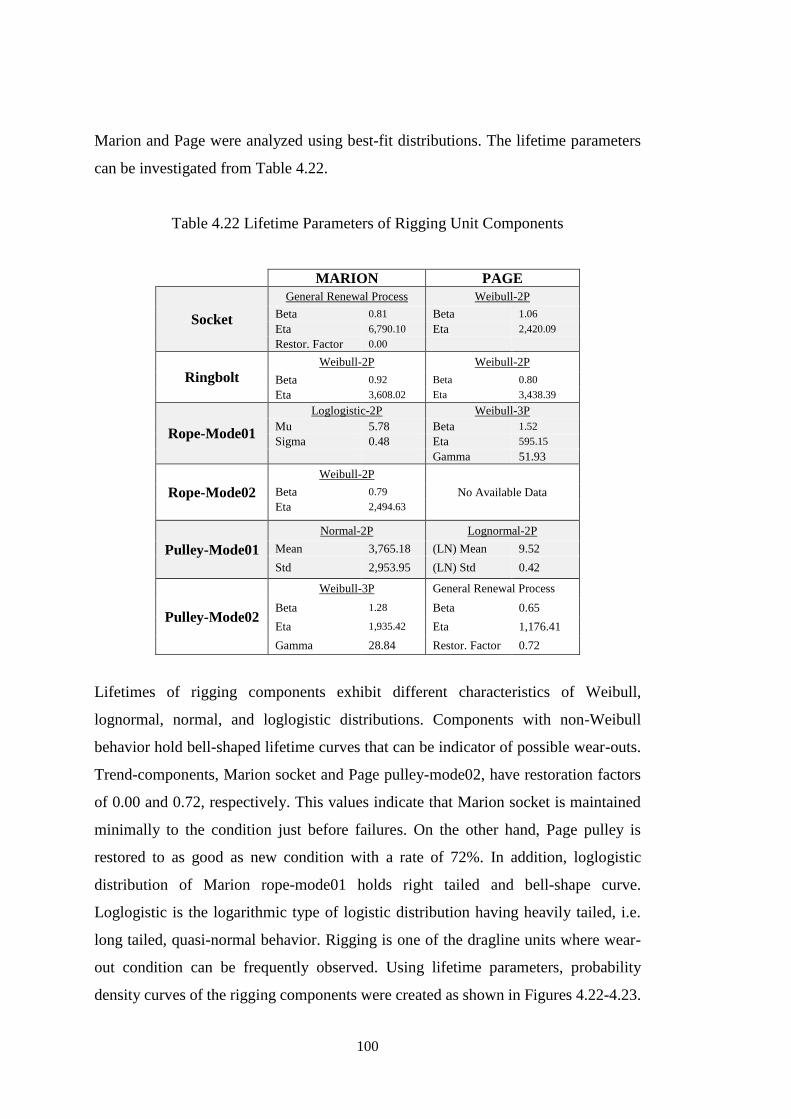
100

Marion and Page were analyzed using best-fit distributions. The lifetime parameters

can be investigated from Table 4.22.

Table 4.22 Lifetime Parameters of Rigging Unit Components

MARION PAGE

Socket

General Renewal Process Weibull-2P

Beta 0.81 Beta 1.06

Eta 6,790.10 Eta 2,420.09

Restor. Factor 0.00

Ringbolt Weibull-2P Weibull-2P

Beta 0.92 Beta 0.80

Eta 3,608.02 Eta 3,438.39

Rope-Mode01

Loglogistic-2P Weibull-3P

Mu 5.78 Beta 1.52

Sigma 0.48 Eta 595.15

Gamma 51.93

Rope-Mode02

Weibull-2P

No Available Data Beta 0.79

Eta 2,494.63

Pulley-Mode01

Normal-2P Lognormal-2P

Mean 3,765.18 (LN) Mean 9.52

Std 2,953.95 (LN) Std 0.42

Pulley-Mode02

Weibull-3P General Renewal Process

Beta 1.28 Beta 0.65

Eta 1,935.42 Eta 1,176.41

Gamma 28.84 Restor. Factor 0.72

Lifetimes of rigging components exhibit different characteristics of Weibull,

lognormal, normal, and loglogistic distributions. Components with non-Weibull

behavior hold bell-shaped lifetime curves that can be indicator of possible wear-outs.

Trend-components, Marion socket and Page pulley-mode02, have restoration factors

of 0.00 and 0.72, respectively. This values indicate that Marion socket is maintained

minimally to the condition just before failures. On the other hand, Page pulley is

restored to as good as new condition with a rate of 72%. In addition, loglogistic

distribution of Marion rope-mode01 holds right tailed and bell-shape curve.

Loglogistic is the logarithmic type of logistic distribution having heavily tailed, i.e.

long tailed, quasi-normal behavior. Rigging is one of the dragline units where wear-

out condition can be frequently observed. Using lifetime parameters, probability

density curves of the rigging components were created as shown in Figures 4.22-4.23.

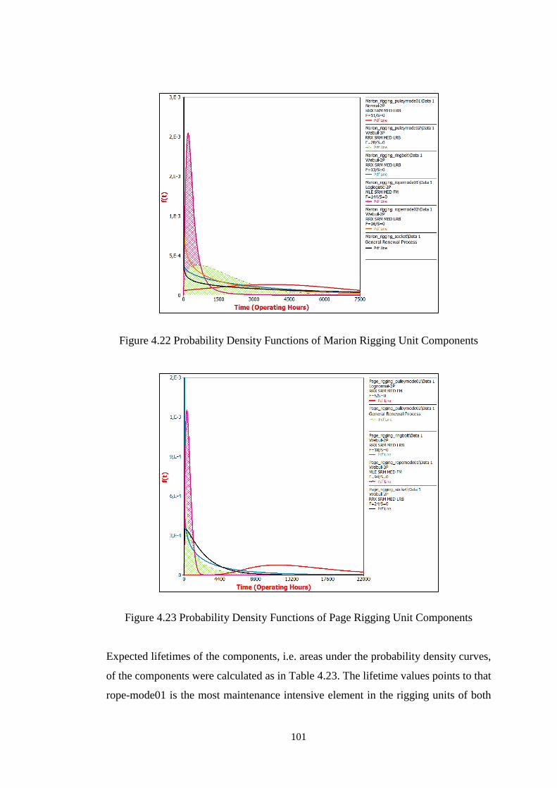
101

Figure 4.22 Probability Density Functions of Marion Rigging Unit Components

Figure 4.23 Probability Density Functions of Page Rigging Unit Components

Expected lifetimes of the components, i.e. areas under the probability density curves,

of the components were calculated as in Table 4.23. The lifetime values points to that

rope-mode01 is the most maintenance intensive element in the rigging units of both

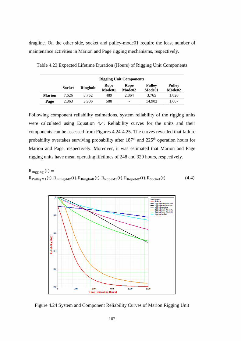
102

dragline. On the other side, socket and pulley-mode01 require the least number of

maintenance activities in Marion and Page rigging mechanisms, respectively.

Table 4.23 Expected Lifetime Duration (Hours) of Rigging Unit Components

Rigging Unit Components

Socket Ringbolt Rope

Mode01

Rope

Mode02

Pulley

Mode01

Pulley

Mode02

Marion 7,626 3,752 489 2,864 3,765 1,820

Page 2,363 3,906 588 - 14,902 1,607

Following component reliability estimations, system reliability of the rigging units

were calculated using Equation 4.4. Reliability curves for the units and their

components can be assessed from Figures 4.24-4.25. The curves revealed that failure

probability overtakes surviving probability after 187th and 225th operation hours for

Marion and Page, respectively. Moreover, it was estimated that Marion and Page

rigging units have mean operating lifetimes of 248 and 320 hours, respectively.

RRigging (t) =

RPulleyM1(t). RPulleyM2(t). RRingbolt(t). RRopeM1(t). RRopeM2(t). RSocket(t) (4.4)

Figure 4.24 System and Component Reliability Curves of Marion Rigging Unit

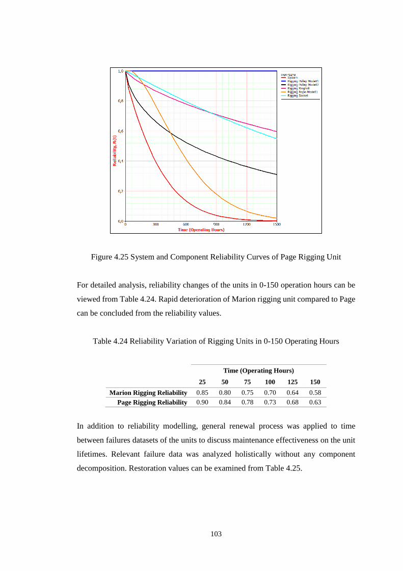
103

Figure 4.25 System and Component Reliability Curves of Page Rigging Unit

For detailed analysis, reliability changes of the units in 0-150 operation hours can be

viewed from Table 4.24. Rapid deterioration of Marion rigging unit compared to Page

can be concluded from the reliability values.

Table 4.24 Reliability Variation of Rigging Units in 0-150 Operating Hours

Time (Operating Hours)

25 50 75 100 125 150

Marion Rigging Reliability 0.85 0.80 0.75 0.70 0.64 0.58

Page Rigging Reliability 0.90 0.84 0.78 0.73 0.68 0.63

In addition to reliability modelling, general renewal process was applied to time

between failures datasets of the units to discuss maintenance effectiveness on the unit

lifetimes. Relevant failure data was analyzed holistically without any component

decomposition. Restoration values can be examined from Table 4.25.

104

Table 4.25 Maintenance Restoration Effectiveness for Rigging Units

General Renewal Function Parameters

Shape (Beta) Lambda Scale (Eta) Degree of Repair Restoration Factor

Marion 1.24 8.00E-4 292.12 0.00 1.00

Page 1.19 8.00E-4 407.37 0.00 1.00

Restoration factors in Table 4.25 revealed that maintenance policy applied for rigging

mechanisms restores these units to as good as new condition.

4.2.5 Machinery House Unit

Dragline machinery house (MH) is composed of: i) motors to perform hoisting,

dragging, swing, and walking movements, ii) relevant generators, iii) lubrication unit

for oil feeding, and iv) air conditioning parts. Unlike the other units, machinery house

covers plenty of electrical appurtenances in order to ensure power requirement of

dragline. It is the transition area where electrical energy is converted to mechanical

energy to sustain the functionality of dragline. Failure of machinery house elements

may cause longer downtimes compared to downtimes induced by the other units.

Dragline machinery house includes capital-intensive components which are rarely

renewed during dragline lifetime period. They are repairable mechanisms and

maintained via inspecting and recovering electrical and mechanical elements

embedded in the mechanisms. Therefore, lifetime trend behaviors of all components

were analyzed prior to reliability estimation.

Lifetime trends of the components were investigated graphically (Figures 4.26-4.27)

and quantitatively (Tables 4.26-4.27). Test results showed that there is a strong

evidence of lifetime trend for generator and motor components in Page machinery

house. On the other hand, hypothesis tests indicated that there is no any lifetime trend

for Marion machinery house components. Air conditioning is excluded in the analyses

for Page since there is no any available failure data.

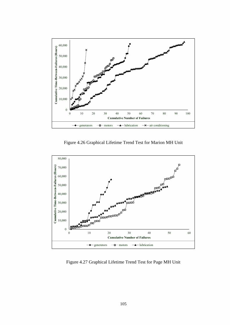
105

Figure 4.26 Graphical Lifetime Trend Test for Marion MH Unit

Figure 4.27 Graphical Lifetime Trend Test for Page MH Unit

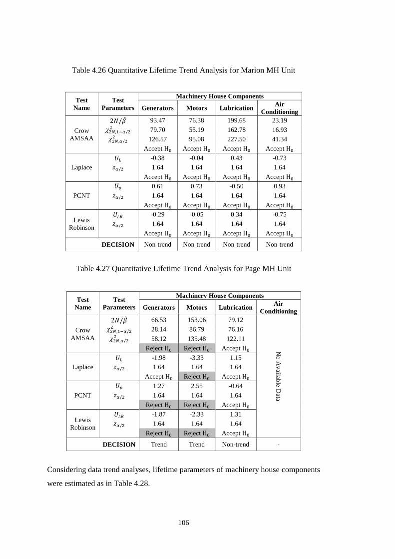
106

Table 4.26 Quantitative Lifetime Trend Analysis for Marion MH Unit

Test

Name

Test

Parameters

Machinery House Components

Generators Motors Lubrication Air

Conditioning

Crow

AMSAA

2𝑁/�̂� 93.47 76.38 199.68 23.19

𝜒2𝑁,1−𝛼/22 79.70 55.19 162.78 16.93

𝜒2𝑁,𝛼/22 126.57 95.08 227.50 41.34

Accept H0 Accept H0 Accept H0 Accept H0

Laplace

𝑈𝐿 -0.38 -0.04 0.43 -0.73

𝑧𝛼/2 1.64 1.64 1.64 1.64

Accept H0 Accept H0 Accept H0 Accept H0

PCNT

𝑈𝑝 0.61 0.73 -0.50 0.93

𝑧𝛼/2 1.64 1.64 1.64 1.64

Accept H0 Accept H0 Accept H0 Accept H0

Lewis

Robinson

𝑈𝐿𝑅 -0.29 -0.05 0.34 -0.75

𝑧𝛼/2 1.64 1.64 1.64 1.64

Accept H0 Accept H0 Accept H0 Accept H0

DECISION Non-trend Non-trend Non-trend Non-trend

Table 4.27 Quantitative Lifetime Trend Analysis for Page MH Unit

Test

Name

Test

Parameters

Machinery House Components

Generators Motors Lubrication Air

Conditioning

Crow

AMSAA

2𝑁/�̂� 66.53 153.06 79.12

No

Av

ailable D

ata

𝜒2𝑁,1−𝛼/22 28.14 86.79 76.16

𝜒2𝑁,𝛼/22 58.12 135.48 122.11

Reject H0 Reject H0 Accept H0

Laplace

𝑈𝐿 -1.98 -3.33 1.15

𝑧𝛼/2 1.64 1.64 1.64

Accept H0 Reject H0 Accept H0

PCNT

𝑈𝑝 1.27 2.55 -0.64

𝑧𝛼/2 1.64 1.64 1.64

Reject H0 Reject H0 Accept H0

Lewis

Robinson

𝑈𝐿𝑅 -1.87 -2.33 1.31

𝑧𝛼/2 1.64 1.64 1.64

Reject H0 Reject H0 Accept H0

DECISION Trend Trend Non-trend -

Considering data trend analyses, lifetime parameters of machinery house components

were estimated as in Table 4.28.

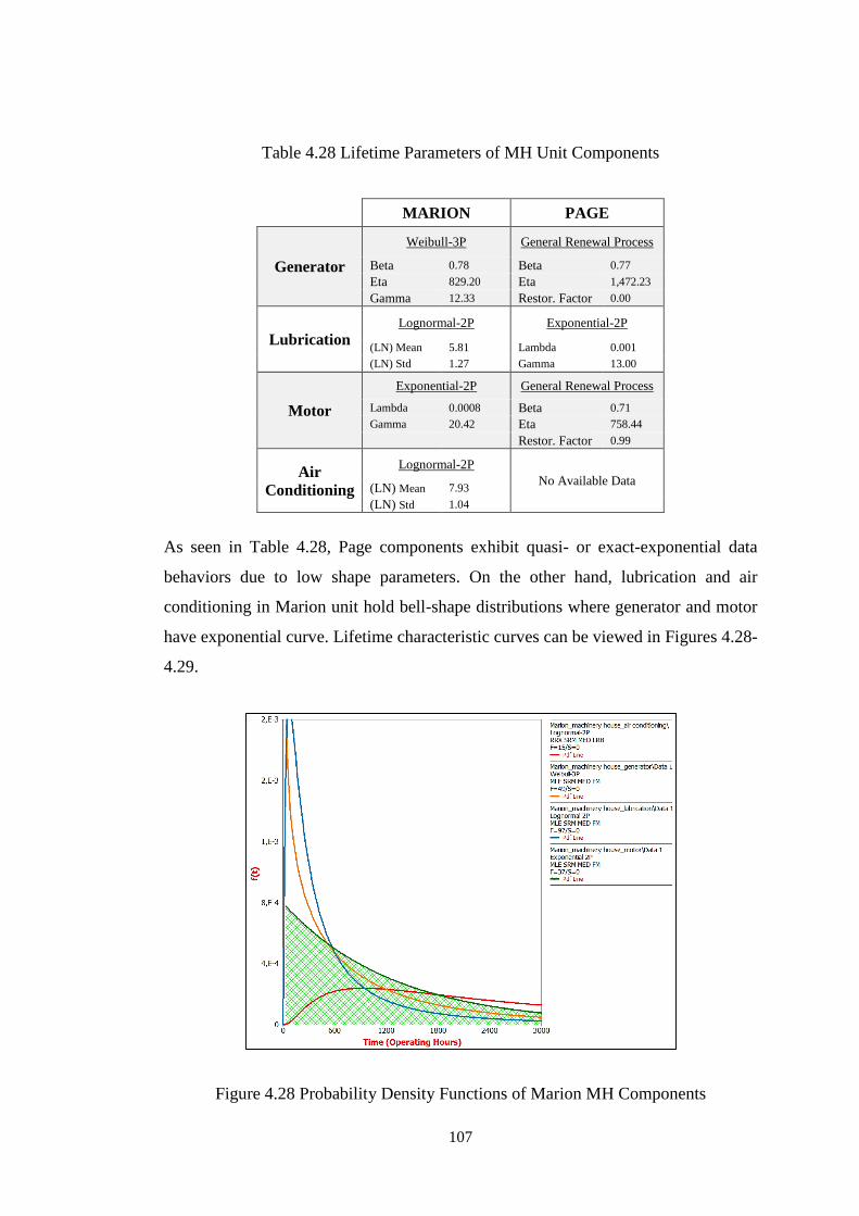
107

Table 4.28 Lifetime Parameters of MH Unit Components

MARION PAGE

Generator

Weibull-3P General Renewal Process

Beta 0.78 Beta 0.77

Eta 829.20 Eta 1,472.23

Gamma 12.33 Restor. Factor 0.00

Lubrication Lognormal-2P Exponential-2P

(LN) Mean 5.81 Lambda 0.001

(LN) Std 1.27 Gamma 13.00

Motor

Exponential-2P General Renewal Process

Lambda 0.0008 Beta 0.71

Gamma 20.42 Eta 758.44

Restor. Factor 0.99

Air

Conditioning

Lognormal-2P

No Available Data (LN) Mean 7.93

(LN) Std 1.04

As seen in Table 4.28, Page components exhibit quasi- or exact-exponential data

behaviors due to low shape parameters. On the other hand, lubrication and air

conditioning in Marion unit hold bell-shape distributions where generator and motor

have exponential curve. Lifetime characteristic curves can be viewed in Figures 4.28-

4.29.

Figure 4.28 Probability Density Functions of Marion MH Components

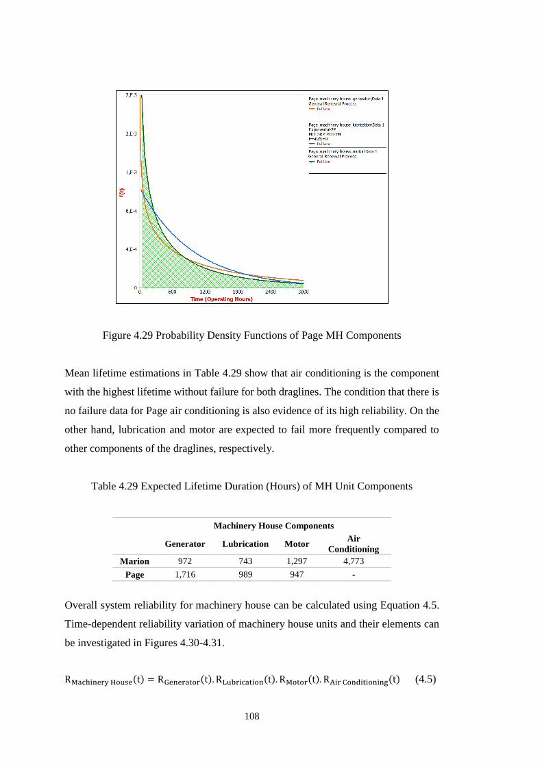
108

Figure 4.29 Probability Density Functions of Page MH Components

Mean lifetime estimations in Table 4.29 show that air conditioning is the component

with the highest lifetime without failure for both draglines. The condition that there is

no failure data for Page air conditioning is also evidence of its high reliability. On the

other hand, lubrication and motor are expected to fail more frequently compared to

other components of the draglines, respectively.

Table 4.29 Expected Lifetime Duration (Hours) of MH Unit Components

Machinery House Components

Generator Lubrication Motor Air

Conditioning

Marion 972 743 1,297 4,773

Page 1,716 989 947 -

Overall system reliability for machinery house can be calculated using Equation 4.5.

Time-dependent reliability variation of machinery house units and their elements can

be investigated in Figures 4.30-4.31.

RMachinery House(t) = RGenerator(t). RLubrication(t). RMotor(t). RAir Conditioning(t) (4.5)

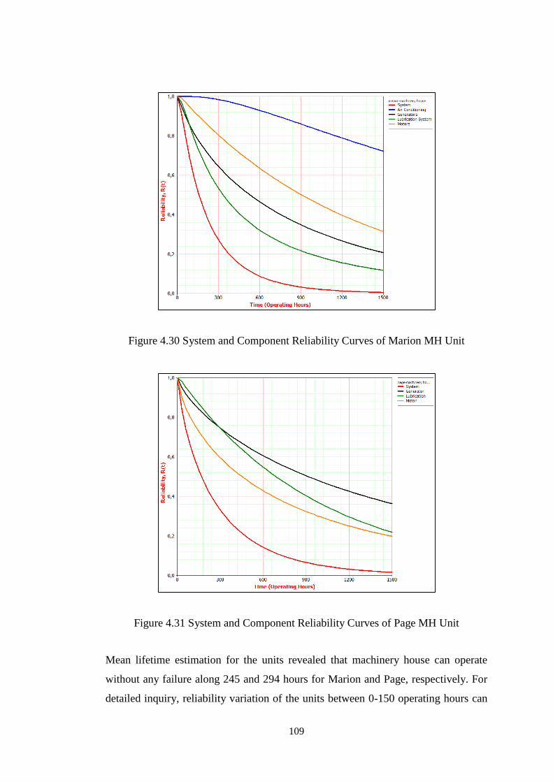
109

Figure 4.30 System and Component Reliability Curves of Marion MH Unit

Figure 4.31 System and Component Reliability Curves of Page MH Unit

Mean lifetime estimation for the units revealed that machinery house can operate

without any failure along 245 and 294 hours for Marion and Page, respectively. For

detailed inquiry, reliability variation of the units between 0-150 operating hours can

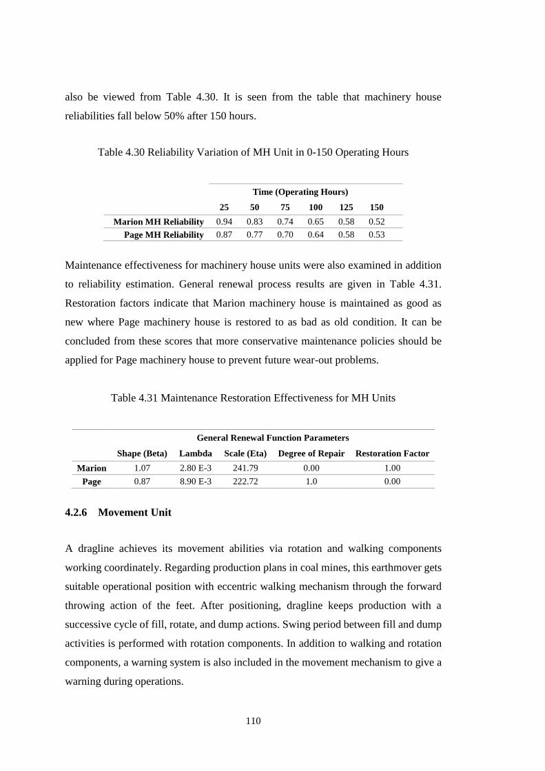
110

also be viewed from Table 4.30. It is seen from the table that machinery house

reliabilities fall below 50% after 150 hours.

Table 4.30 Reliability Variation of MH Unit in 0-150 Operating Hours

Time (Operating Hours)

25 50 75 100 125 150

Marion MH Reliability 0.94 0.83 0.74 0.65 0.58 0.52

Page MH Reliability 0.87 0.77 0.70 0.64 0.58 0.53

Maintenance effectiveness for machinery house units were also examined in addition

to reliability estimation. General renewal process results are given in Table 4.31.

Restoration factors indicate that Marion machinery house is maintained as good as

new where Page machinery house is restored to as bad as old condition. It can be

concluded from these scores that more conservative maintenance policies should be

applied for Page machinery house to prevent future wear-out problems.

Table 4.31 Maintenance Restoration Effectiveness for MH Units

General Renewal Function Parameters

Shape (Beta) Lambda Scale (Eta) Degree of Repair Restoration Factor

Marion 1.07 2.80 E-3 241.79 0.00 1.00

Page 0.87 8.90 E-3 222.72 1.0 0.00

4.2.6 Movement Unit

A dragline achieves its movement abilities via rotation and walking components

working coordinately. Regarding production plans in coal mines, this earthmover gets

suitable operational position with eccentric walking mechanism through the forward

throwing action of the feet. After positioning, dragline keeps production with a

successive cycle of fill, rotate, and dump actions. Swing period between fill and dump

activities is performed with rotation components. In addition to walking and rotation

components, a warning system is also included in the movement mechanism to give a

warning during operations.

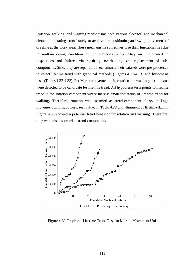
111

Rotation, walking, and warning mechanisms hold various electrical and mechanical

elements operating coordinately to achieve the positioning and swing movement of

dragline at the work area. These mechanisms sometimes lose their functionalities due

to malfunctioning condition of the sub-constituents. They are maintained in

inspections and failures via repairing, overhauling, and replacement of sub-

components. Since they are repairable mechanisms, their datasets were pre-processed

to detect lifetime trend with graphical methods (Figures 4.32-4.33) and hypothesis

tests (Tables 4.32-4.33). For Marion movement unit, rotation and walking mechanisms

were detected to be candidate for lifetime trend. All hypothesis tests points to lifetime

trend in the rotation component where there is small indication of lifetime trend for

walking. Therefore, rotation was assumed as trend-component alone. In Page

movement unit, hypothesis test values in Table 4.33 and alignment of lifetime data in

Figure 4.33 showed a potential trend behavior for rotation and warning. Therefore,

they were also assumed as trend-components.

Figure 4.32 Graphical Lifetime Trend Test for Marion Movement Unit

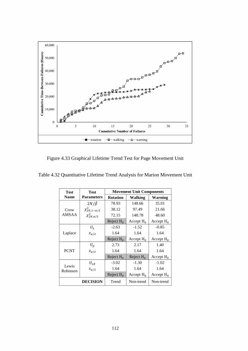
112

Figure 4.33 Graphical Lifetime Trend Test for Page Movement Unit

Table 4.32 Quantitative Lifetime Trend Analysis for Marion Movement Unit

Test

Name

Test

Parameters

Movement Unit Components

Rotation Walking Warning

Crow

AMSAA

2𝑁/�̂� 78.93 148.66 35.01

𝜒2𝑁,1−𝛼/22 38.12 97.49 21.66

𝜒2𝑁,𝛼/22 72.15 148.78 48.60

Reject H0 Accept H0 Accept H0

Laplace

𝑈𝐿 -2.63 -1.52 -0.85

𝑧𝛼/2 1.64 1.64 1.64

Reject H0 Accept H0 Accept H0

PCNT

𝑈𝑝 2.73 2.17 1.40

𝑧𝛼/2 1.64 1.64 1.64

Reject H0 Reject H0 Accept H0

Lewis

Robinson

𝑈𝐿𝑅 -3.02 -1.30 -1.02

𝑧𝛼/2 1.64 1.64 1.64

Reject H0 Accept H0 Accept H0

DECISION Trend Non-trend Non-trend

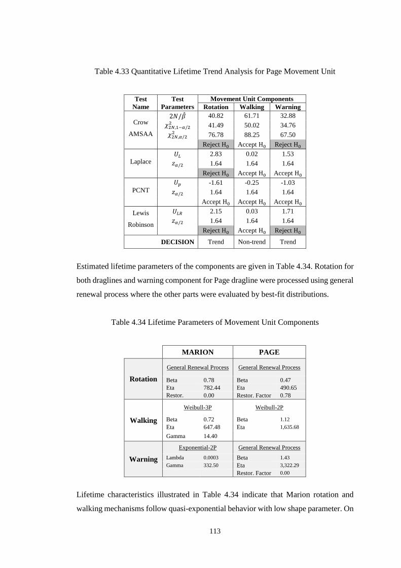
113

Table 4.33 Quantitative Lifetime Trend Analysis for Page Movement Unit

Test

Name

Test

Parameters

Movement Unit Components

Rotation Walking Warning

Crow

AMSAA

2𝑁/�̂� 40.82 61.71 32.88

𝜒2𝑁,1−𝛼/22 41.49 50.02 34.76

𝜒2𝑁,𝛼/22 76.78 88.25 67.50

Reject H0 Accept H0 Reject H0

Laplace 𝑈𝐿 2.83 0.02 1.53

𝑧𝛼/2 1.64 1.64 1.64

Reject H0 Accept H0 Accept H0

PCNT

𝑈𝑝 -1.61 -0.25 -1.03

𝑧𝛼/2 1.64 1.64 1.64

Accept H0 Accept H0 Accept H0

Lewis

Robinson

𝑈𝐿𝑅 2.15 0.03 1.71

𝑧𝛼/2 1.64 1.64 1.64

Reject H0 Accept H0 Reject H0

DECISION Trend Non-trend Trend

Estimated lifetime parameters of the components are given in Table 4.34. Rotation for

both draglines and warning component for Page dragline were processed using general

renewal process where the other parts were evaluated by best-fit distributions.

Table 4.34 Lifetime Parameters of Movement Unit Components

MARION PAGE

Rotation

General Renewal Process General Renewal Process

Beta 0.78 Beta 0.47

Eta 782.44 Eta 490.65

Restor.

Factor 0.00 Restor. Factor 0.78

Walking

Weibull-3P Weibull-2P

Beta 0.72 Beta 1.12

Eta 647.48 Eta 1,635.68

Gamma 14.40

Warning

Exponential-2P General Renewal Process

Lambda 0.0003 Beta 1.43

Gamma 332.50 Eta 3,322.29

Restor. Factor 0.00

Lifetime characteristics illustrated in Table 4.34 indicate that Marion rotation and

walking mechanisms follow quasi-exponential behavior with low shape parameter. On

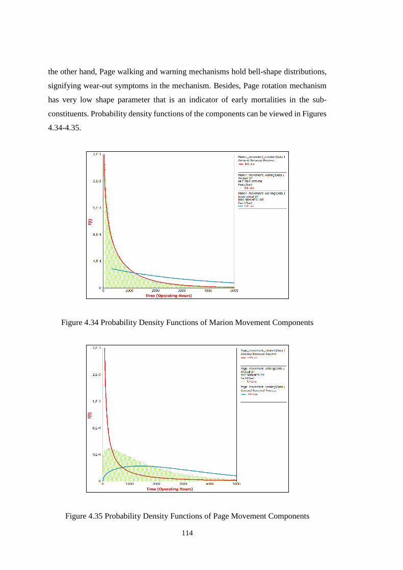
114

the other hand, Page walking and warning mechanisms hold bell-shape distributions,

signifying wear-out symptoms in the mechanism. Besides, Page rotation mechanism

has very low shape parameter that is an indicator of early mortalities in the sub-

constituents. Probability density functions of the components can be viewed in Figures

4.34-4.35.

Figure 4.34 Probability Density Functions of Marion Movement Components

Figure 4.35 Probability Density Functions of Page Movement Components

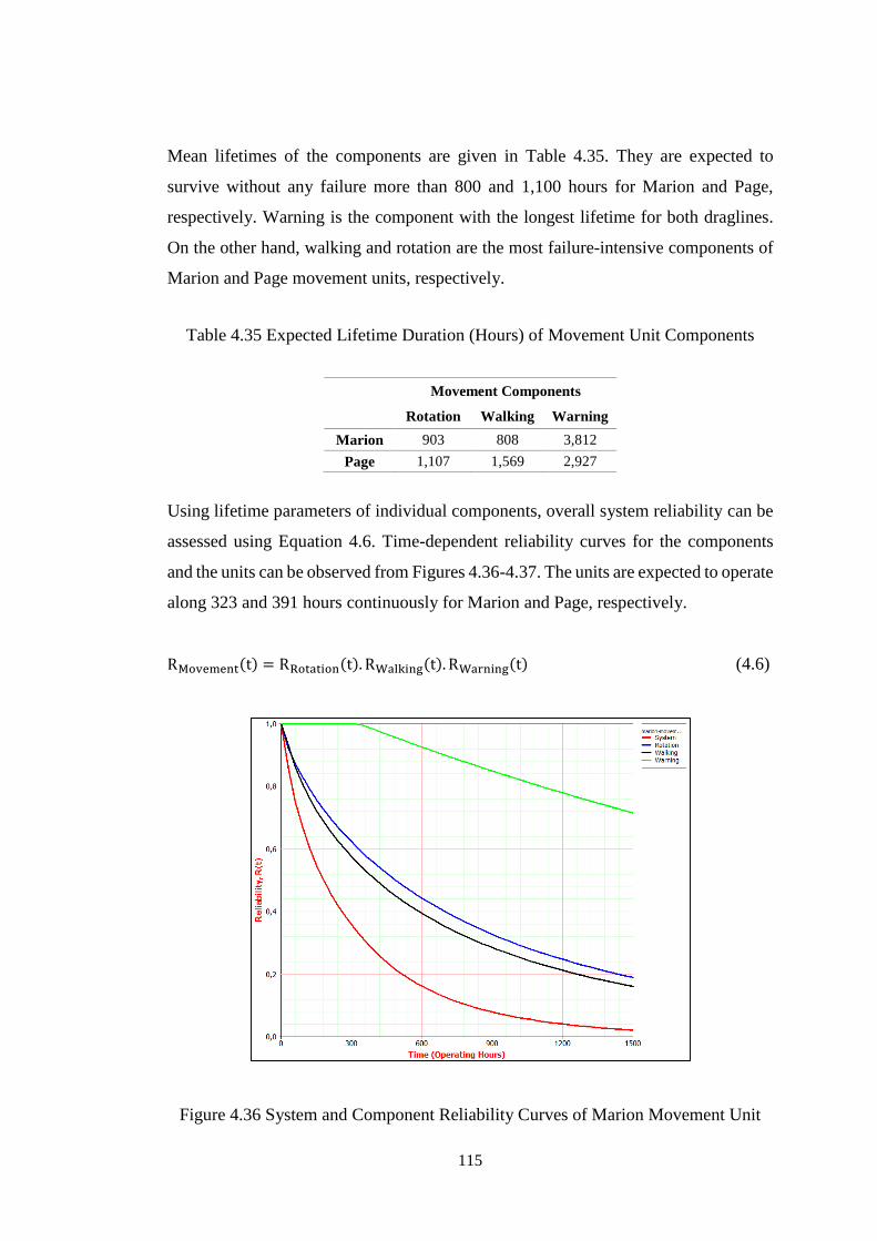
115

Mean lifetimes of the components are given in Table 4.35. They are expected to

survive without any failure more than 800 and 1,100 hours for Marion and Page,

respectively. Warning is the component with the longest lifetime for both draglines.

On the other hand, walking and rotation are the most failure-intensive components of

Marion and Page movement units, respectively.

Table 4.35 Expected Lifetime Duration (Hours) of Movement Unit Components

Movement Components

Rotation Walking Warning

Marion 903 808 3,812

Page 1,107 1,569 2,927

Using lifetime parameters of individual components, overall system reliability can be

assessed using Equation 4.6. Time-dependent reliability curves for the components

and the units can be observed from Figures 4.36-4.37. The units are expected to operate

along 323 and 391 hours continuously for Marion and Page, respectively.

RMovement(t) = RRotation(t). RWalking(t). RWarning(t) (4.6)

Figure 4.36 System and Component Reliability Curves of Marion Movement Unit

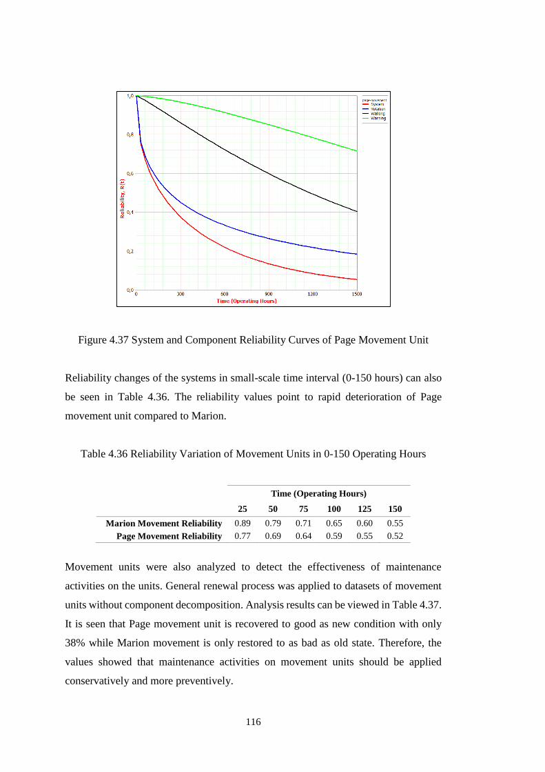
116

Figure 4.37 System and Component Reliability Curves of Page Movement Unit

Reliability changes of the systems in small-scale time interval (0-150 hours) can also

be seen in Table 4.36. The reliability values point to rapid deterioration of Page

movement unit compared to Marion.

Table 4.36 Reliability Variation of Movement Units in 0-150 Operating Hours

Time (Operating Hours)

25 50 75 100 125 150

Marion Movement Reliability 0.89 0.79 0.71 0.65 0.60 0.55

Page Movement Reliability 0.77 0.69 0.64 0.59 0.55 0.52

Movement units were also analyzed to detect the effectiveness of maintenance

activities on the units. General renewal process was applied to datasets of movement

units without component decomposition. Analysis results can be viewed in Table 4.37.

It is seen that Page movement unit is recovered to good as new condition with only

38% while Marion movement is only restored to as bad as old state. Therefore, the

values showed that maintenance activities on movement units should be applied

conservatively and more preventively.

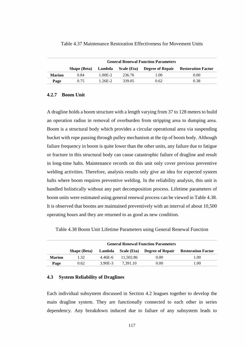
117

Table 4.37 Maintenance Restoration Effectiveness for Movement Units

General Renewal Function Parameters

Shape (Beta) Lambda Scale (Eta) Degree of Repair Restoration Factor

Marion 0.84 1.00E-2 236.76 1.00 0.00

Page 0.75 1.26E-2 339.05 0.62 0.38

4.2.7 Boom Unit

A dragline holds a boom structure with a length varying from 37 to 128 meters to build

an operation radius in removal of overburden from stripping area to dumping area.

Boom is a structural body which provides a circular operational area via suspending

bucket with rope passing through pulley mechanism at the tip of boom body. Although

failure frequency in boom is quite lower than the other units, any failure due to fatigue

or fracture in this structural body can cause catastrophic failure of dragline and result

in long-time halts. Maintenance records on this unit only cover previous preventive

welding activities. Therefore, analysis results only give an idea for expected system

halts where boom requires preventive welding. In the reliability analysis, this unit is

handled holistically without any part decomposition process. Lifetime parameters of

boom units were estimated using general renewal process can be viewed in Table 4.38.

It is observed that booms are maintained preventively with an interval of about 10,500

operating hours and they are returned to as good as new condition.

Table 4.38 Boom Unit Lifetime Parameters using General Renewal Function

General Renewal Function Parameters

Shape (Beta) Lambda Scale (Eta) Degree of Repair Restoration Factor

Marion 1.32 4.46E-6 11,502.86 0.00 1.00

Page 0.62 3.90E-3 7,391.10 0.00 1.00

4.3 System Reliability of Draglines

Each individual subsystem discussed in Section 4.2 leagues together to develop the

main dragline system. They are functionally connected to each other in series

dependency. Any breakdown induced due to failure of any subsystem leads to

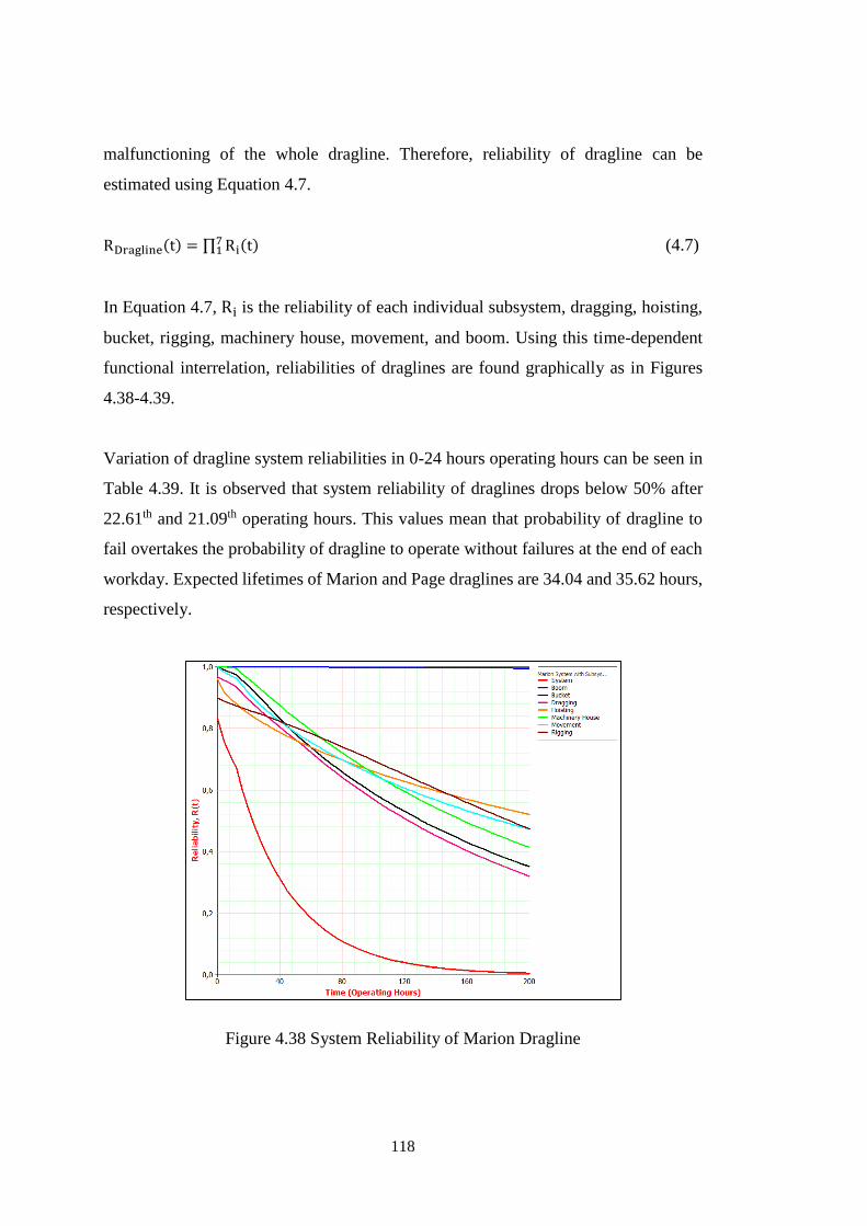
118

malfunctioning of the whole dragline. Therefore, reliability of dragline can be

estimated using Equation 4.7.

RDragline(t) = ∏ Ri(t)71 (4.7)

In Equation 4.7, Ri is the reliability of each individual subsystem, dragging, hoisting,

bucket, rigging, machinery house, movement, and boom. Using this time-dependent

functional interrelation, reliabilities of draglines are found graphically as in Figures

4.38-4.39.

Variation of dragline system reliabilities in 0-24 hours operating hours can be seen in

Table 4.39. It is observed that system reliability of draglines drops below 50% after

22.61th and 21.09th operating hours. This values mean that probability of dragline to

fail overtakes the probability of dragline to operate without failures at the end of each

workday. Expected lifetimes of Marion and Page draglines are 34.04 and 35.62 hours,

respectively.

Figure 4.38 System Reliability of Marion Dragline

119

Figure 4.39 System Reliability of Page Dragline

Table 4.39 Time-Dependent Reliability and Mean Lifetimes of Draglines

Operation Time (Hour)

4 8 12 16 20 24

Marion System Reliability 0.76 0.71 0.67 0.60 0.54 0.48

Page System Reliability 0.80 0.71 0.64 0.57 0.51 0.47

Although previous subsystem analyses in Sections 4.2 showed that subsystems for

both dragline exhibit different characteristics, Table 4.39 stated that functionality of

overall systems exhibit similar deterioration rates. This condition proves importance

of deductive reliability analysis which concerns top-to-bottom component-based

reliability modelling. If dragline reliability in the study was handled holistically

without component decomposition, it would be concluded that dragline components

have similar reliability behavior. Regarding this assumption, preventive maintenance

policies would be generated commonly for both dragline. However, root-cause

reliability analysis in the study showed that main weaknesses in the mechanisms

differs machine to machine even they are operated in similar operations. In this sense,

Section 5 will present optimization of maintenance policies of both draglines

considering their component characteristics.

120

121

5. PREVENTIVE MAINTENANCE POLICIES FOR WALKING

DRAGLINES

5.1 Introduction

Preventive maintenance policies allow decision makers to reduce maintenance costs

and to control health of machinery components via optimizing maintenance actions in

finite or infinite time intervals. Scope of the policies may cover optimizing inspection

periods, determining preventive replacement criterion for system components, keeping

system reliability over prescribed limits or developing breakdown maintenance policy.

Moreover, these policies may be modelled mathematically to maximize the values of

profit, reliability, and availability or minimize cost or downtime amounts in prescribed

intervals. This study considered cost as a minimization criterion since it is a rational

and realistic parameter to measure direct and indirect economic consequences of

system halts. Initially, annual failure profiles of the draglines were built up for current

maintenance policy using Monte Carlo simulation. In optimization part, feasibility of

preventive component replacements was discussed first via age replacement policies.

Replacement interval curves were drawn for changing preventive and corrective costs.

Then, a time-counting algorithm was created considering replacement decisions,

random lifetime and repair behaviors of components, economic consequences of

failures, and scheduled compulsory halts. A sensitivity analysis was performed in the

algorithm to find out optimal inspection interval which minimizes overall cost of

maintenance. In addition to the algorithm, a risk-based reliability allocation model was

constructed to measure cost-effective maintenance criticalities of individual

components. This model provided a perspective about which component reliability

should be improved with priority. The methodology applied in this section can be

viewed in Figure 5.1.

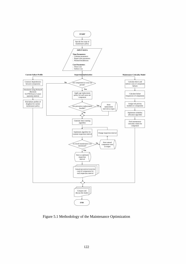
122

START

Specify the scope of

maintenance policy

INPUT DATA

Time Parameters

Lifetime parameters

Repair time parameters

Planned breakdowns

Cost Parameters

Direct cost

Indirect cost

Apply age replacement

policy for each wear-out

component

Are preventive replacements

feasible?

Generate time-counting

algorithm

Are components in wear-out

period?

Calculate direct and

indirect costs of component

failures

Calculate failure

frequencies of components

Assign risk priority

numbers to components

Implement reliability

allocation algorithm

END

No

Yes

No

Maintenance Criticality Model

Construct dependencies

between components

Simulation using Reliasoft

Blocksim

for 8766 hours (1-year)

operation interval

Find failure profiles of

draglines for current

maintenance policy

Implement algortihm for

constant inspection intervalChange inspection interval

Is overall maintenance cost

minimized?

Store annual

component costs

as output

Store as optimum

inspection

interval

Annual preventive/corrective

costs of components for

each inspection interval

Compare and

discuss the results

Find maintenance

criticality values for

component

Store

replacement

intervals as input

Yes

Yes

No

Current Failure Profile Inspection Optimization

Figure 5.1 Methodology of the Maintenance Optimization

123

5.2 Current Conditions and Economic Aspects of the Maintenance Activities in

Tunçbilek Coal Mine

In the literature, case studies about maintenance policies are generally based on the

maximization of operational factors such as, reliability and availability, without

considering cost effect. Maintenance cost analyses are rarely observed in the literature

since cost values can be acquired rarely or cost-free models are easy to implement.

However, cost is an important parameter in order to build realistic and applicable

maintenance models in industries. This study utilized cost values in the maintenance

optimization part. In this basis, this section informed about the details of current

maintenance applications for the draglines in Tunçbilek coal mine and direct and

indirect economic consequences of component failures. In addition, a simulation was

generated using Monte Carlo technique to reveal the current failure profiles of the

draglines.

General conditions of dragline operations and maintenance activities at the mine site

can be assessed as follows:

i. Draglines operate in 3 shifts with 8-hours working periods.

ii. In each shift, there is a compulsory break of 30 minutes due to legal worker rights.

Therefore, effective utilization time of a dragline is 22.5 hours a day.

iii. Operative conditions of draglines can be halted due to: a) component failures, b)

regular inspections, c) interruptions on energy transmission line, d) unfavorable

weather conditions, e) lack of sufficient maintenance staff, and f) problems in

acquisition of spare parts.

iv. Draglines are maintained in three main ways: a) corrective maintenance when

component is failed, b) 8 hours regular inspections every 160 hours, and c) general

shutdown maintenance for detailed maintenance and overhauling.

Cost of any maintenance activity can be measured using direct and indirect factors.

Direct cost is physical cost of activity paid directly to the collaborators such as, spare

part suppliers, maintenance staff, energy providers, and machine hiring companies. On

the other hand, indirect cost is the economic consequences of any failure due to

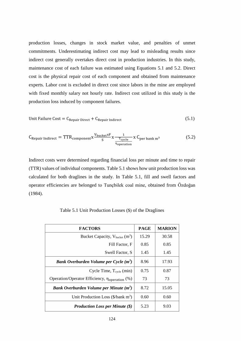
124

production losses, changes in stock market value, and penalties of unmet

commitments. Underestimating indirect cost may lead to misleading results since

indirect cost generally overtakes direct cost in production industries. In this study,

maintenance cost of each failure was estimated using Equations 5.1 and 5.2. Direct

cost is the physical repair cost of each component and obtained from maintenance

experts. Labor cost is excluded in direct cost since labors in the mine are employed

with fixed monthly salary not hourly rate. Indirect cost utilized in this study is the

production loss induced by component failures.

Unit Failure Cost = CRepair Direct + CRepair Indirect (5.1)

CRepair Indirect = TTRcomponentxVbucketxF

Sx

1Tcycle

ηoperation

x Cper bank m3 (5.2)

Indirect costs were determined regarding financial loss per minute and time to repair

(TTR) values of individual components. Table 5.1 shows how unit production loss was

calculated for both draglines in the study. In Table 5.1, fill and swell factors and

operator efficiencies are belonged to Tunçbilek coal mine, obtained from Özdoğan

(1984).

Table 5.1 Unit Production Losses ($) of the Draglines

FACTORS PAGE MARION

Bucket Capacity, Vbucket (m3) 15.29 30.58

Fill Factor, F 0.85 0.85

Swell Factor, S 1.45 1.45

Bank Overburden Volume per Cycle (m3) 8.96 17.93

Cycle Time, Tcycle (min) 0.75 0.87

Operation/Operator Efficiency, ηoperation (%) 73 73

Bank Overburden Volume per Minute (m3) 8.72 15.05

Unit Production Loss ($/bank m3) 0.60 0.60

Production Loss per Minute ($) 5.23 9.03

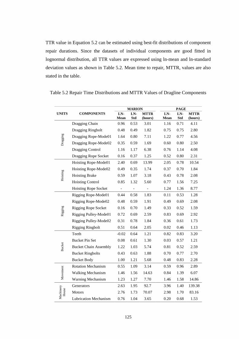
125

TTR value in Equation 5.2 can be estimated using best-fit distributions of component

repair durations. Since the datasets of individual components are good fitted in

lognormal distribution, all TTR values are expressed using ln-mean and ln-standard

deviation values as shown in Table 5.2. Mean time to repair, MTTR, values are also

stated in the table.

Table 5.2 Repair Time Distributions and MTTR Values of Dragline Components

UNITS COMPONENTS

MARION PAGE

LN-

Mean

LN-

Std

MTTR

(hours)

LN-

Mean

LN-

Std

MTTR

(hours)

Dra

ggin

g

Dragging Chain 0.96 0.53 3.01 1.16 0.71 4.11

Dragging Ringbolt 0.48 0.49 1.82 0.75 0.75 2.80

Dragging Rope-Mode01 1.64 0.80 7.11 1.22 0.77 4.56

Dragging Rope-Mode02 0.35 0.59 1.69 0.60 0.80 2.50

Dragging Control 1.16 1.17 6.38 0.76 1.14 4.08

Dragging Rope Socket 0.16 0.37 1.25 0.52 0.80 2.31

Ho

isti

ng

Hoisting Rope-Mode01 2.40 0.69 13.99 2.05 0.78 10.54

Hoisting Rope-Mode02 0.49 0.35 1.74 0.37 0.70 1.84

Hoisting Brake 0.59 1.07 3.18 0.43 0.78 2.08

Hoisting Control 0.85 1.32 5.60 0.77 1.56 7.25

Hoisting Rope Socket - - - 1.24 1.36 8.77

Rig

gin

g

Rigging Rope-Mode01 0.44 0.58 1.83 0.11 0.53 1.28

Rigging Rope-Mode02 0.48 0.59 1.91 0.49 0.69 2.08

Rigging Rope Socket 0.16 0.70 1.49 0.33 0.52 1.59

Rigging Pulley-Mode01 0.72 0.69 2.59 0.83 0.69 2.92

Rigging Pulley-Mode02 0.31 0.78 1.84 0.36 0.61 1.73

Rigging Ringbolt 0.51 0.64 2.05 0.02 0.46 1.13

Buck

et

Teeth -0.02 0.64 1.21 0.82 0.83 3.20

Bucket Pin Set 0.08 0.61 1.30 0.03 0.57 1.21

Bucket Chain Assembly 1.22 1.03 5.74 0.81 0.52 2.59

Bucket Ringbolts 0.43 0.63 1.88 0.70 0.77 2.70

Bucket Body 1.00 1.21 5.68 0.48 0.83 2.28

Mov

emen

t Rotation Mechanism 0.55 1.09 3.14 0.59 0.96 2.89

Walking Mechanism 1.46 1.56 14.63 0.84 1.39 6.07

Warning Mechanism 1.23 1.27 7.70 1.46 1.58 14.86

Mac

hin

ery

Ho

use

Generators 2.63 1.95 92.7 3.96 1.40 139.38

Motors 2.76 1.73 70.07 2.98 1.70 83.16

Lubrication Mechanism 0.76 1.04 3.65 0.20 0.68 1.53

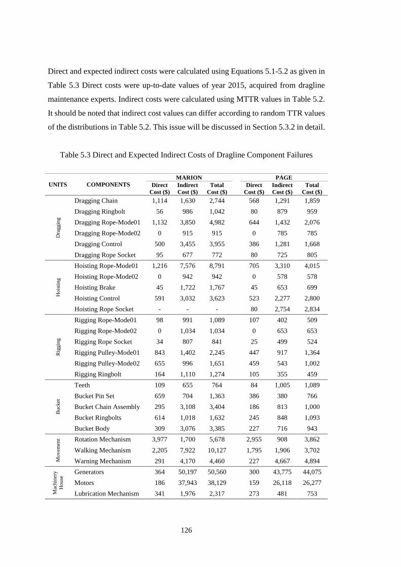
126

Direct and expected indirect costs were calculated using Equations 5.1-5.2 as given in

Table 5.3 Direct costs were up-to-date values of year 2015, acquired from dragline

maintenance experts. Indirect costs were calculated using MTTR values in Table 5.2.

It should be noted that indirect cost values can differ according to random TTR values

of the distributions in Table 5.2. This issue will be discussed in Section 5.3.2 in detail.

Table 5.3 Direct and Expected Indirect Costs of Dragline Component Failures

UNITS COMPONENTS

MARION PAGE

Direct

Cost ($)

Indirect

Cost ($)

Total

Cost ($)

Direct

Cost ($)

Indirect

Cost ($)

Total

Cost ($)

Dra

ggin

g

Dragging Chain 1,114 1,630 2,744 568 1,291 1,859

Dragging Ringbolt 56 986 1,042 80 879 959

Dragging Rope-Mode01 1,132 3,850 4,982 644 1,432 2,076

Dragging Rope-Mode02 0 915 915 0 785 785

Dragging Control 500 3,455 3,955 386 1,281 1,668

Dragging Rope Socket 95 677 772 80 725 805

Ho

isti

ng

Hoisting Rope-Mode01 1,216 7,576 8,791 705 3,310 4,015

Hoisting Rope-Mode02 0 942 942 0 578 578

Hoisting Brake 45 1,722 1,767 45 653 699

Hoisting Control 591 3,032 3,623 523 2,277 2,800

Hoisting Rope Socket - - - 80 2,754 2,834

Rig

gin

g

Rigging Rope-Mode01 98 991 1,089 107 402 509

Rigging Rope-Mode02 0 1,034 1,034 0 653 653

Rigging Rope Socket 34 807 841 25 499 524

Rigging Pulley-Mode01 843 1,402 2,245 447 917 1,364

Rigging Pulley-Mode02 655 996 1,651 459 543 1,002

Rigging Ringbolt 164 1,110 1,274 105 355 459

Buck

et

Teeth 109 655 764 84 1,005 1,089

Bucket Pin Set 659 704 1,363 386 380 766

Bucket Chain Assembly 295 3,108 3,404 186 813 1,000

Bucket Ringbolts 614 1,018 1,632 245 848 1,093

Bucket Body 309 3,076 3,385 227 716 943

Mov

emen

t Rotation Mechanism 3,977 1,700 5,678 2,955 908 3,862

Walking Mechanism 2,205 7,922 10,127 1,795 1,906 3,702

Warning Mechanism 291 4,170 4,460 227 4,667 4,894

Mac

hin

ery

Ho

use

Generators 364 50,197 50,560 300 43,775 44,075

Motors 186 37,943 38,129 159 26,118 26,277

Lubrication Mechanism 341 1,976 2,317 273 481 753

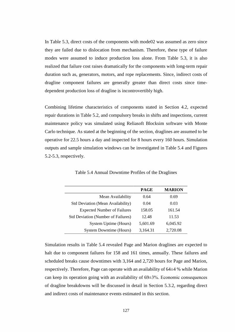
127

In Table 5.3, direct costs of the components with mode02 was assumed as zero since

they are failed due to dislocation from mechanism. Therefore, these type of failure

modes were assumed to induce production loss alone. From Table 5.3, it is also

realized that failure cost raises dramatically for the components with long-term repair

duration such as, generators, motors, and rope replacements. Since, indirect costs of

dragline component failures are generally greater than direct costs since time-

dependent production loss of dragline is incontrovertibly high.

Combining lifetime characteristics of components stated in Section 4.2, expected

repair durations in Table 5.2, and compulsory breaks in shifts and inspections, current

maintenance policy was simulated using Reliasoft Blocksim software with Monte

Carlo technique. As stated at the beginning of the section, draglines are assumed to be

operative for 22.5 hours a day and inspected for 8 hours every 160 hours. Simulation

outputs and sample simulation windows can be investigated in Table 5.4 and Figures

5.2-5.3, respectively.

Table 5.4 Annual Downtime Profiles of the Draglines

PAGE MARION

Mean Availability 0.64 0.69

Std Deviation (Mean Availability) 0.04 0.03

Expected Number of Failures 158.05 161.54

Std Deviation (Number of Failures) 12.48 11.53

System Uptime (Hours) 5,601.69 6,045.92

System Downtime (Hours) 3,164.31 2,720.08

Simulation results in Table 5.4 revealed Page and Marion draglines are expected to

halt due to component failures for 158 and 161 times, annually. These failures and

scheduled breaks cause downtimes with 3,164 and 2,720 hours for Page and Marion,

respectively. Therefore, Page can operate with an availability of 64±4 % while Marion

can keep its operation going with an availability of 69±3%. Economic consequences

of dragline breakdowns will be discussed in detail in Section 5.3.2, regarding direct

and indirect costs of maintenance events estimated in this section.

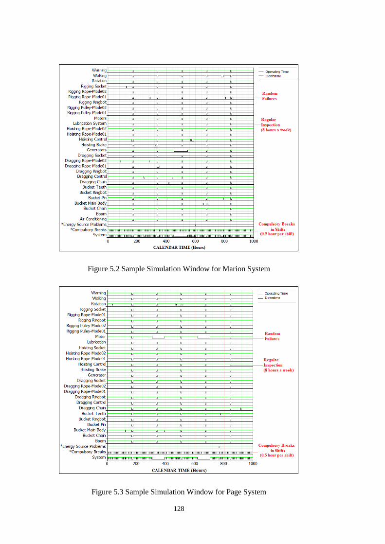
128

Figure 5.2 Sample Simulation Window for Marion System

Figure 5.3 Sample Simulation Window for Page System

129

The simulation assumed that dragline operations are halted for 8 hours every 160 hours

for regular inspection. Number of failures and their occurrence frequency are highly

effected from inspection intervals. Length of inspection intervals is critical to detect

the approaching failures in advance and to maintain components preventively. If

inspections are carried out in short intervals, this condition increases frequency of

system halts due to inspections and resultant production loss. If inspections are

performed in long intervals, then inspections cannot catch defects in components and

production loss due to corrective maintenance again raises dramatically. Therefore,

inspection intervals should be determined in accordance with system characteristics so

that overall economic consequences of maintenance can be reduced. In addition to

inspection intervals, implementation of preventive component replacements during

operation hours is another tool for maintenance policies. Moreover, detection of

maintenance criticalities for components can also be utilized to improve the

maintenance policies. In this sense, understanding about how individual components

contribute to system reliability can raise the awareness about maintenance criticalities

of component. In this basis, Section 5.3 will present cost-effective maintenance

optimization of the draglines via preventive replacement policies, optimization of

inspection intervals and risk-based reliability allocation of the components.

5.3 Cost-Effective Maintenance Optimization of the Draglines

System components deteriorate in operations due to interaction effects such as,

corrosion, wear and tear, cracking, erosion, fatigue, and skin damage. Underestimating

conservative and preventive activities in maintenance policies causes these

components to lose their operational effectiveness with increasing failure rates. In this

sense, reliability-based analyses can help to improve maintenance policies via i)

supporting reliability of subsystems and its constituents above the planned limits and

ii) taking precautions against failure via inspections, repairs, component replacements,

servicing, and overhauling operations.

Components in a system league together in various structural and economical

dependencies. Therefore, integration of reliability to system maintenance policy

requires pre-estimation of components lifetime behavior. Success of the policy may be

130

ensured only with precise estimation of component reliability and identification of

functional relationships between subsystems and components. This section utilized

lifetime characteristics of dragline components estimated in Section 4.2.

In the study, maintenance strategy of draglines was optimized via (i) generating a

decision platform for age-replacements of wear-out components , (ii) development of

an optimization algorithm for inspection intervals to minimize overall maintenance

cost, and (iii) determination of maintenance-critical components with a risk-based

reliability allocation model.

5.3.1 Investigation of Component Replacement Decisions

Preventive replacement decisions in maintenance policies can be handled in two ways

as replacement of capital equipment and replacement of individual component. Since

replacement of dragline is out of scope in this study, it will be focused on the

determination of replacement intervals for critical system components. Preventive

replacement decisions can be applied for components in deterioration period. If a

component exhibits random failure behavior without any aging condition, these parts

are not considered under age-replacement decisions. Prerequisites for the applicability

of age-replacement policies are as follows:

i. The component should be in wear-out period. For Weibull distribution, shape

parameter (𝛽) is good indicator of determining whether component is in early

stages of its lifetime, in its useful lifetime with random failure patterns, or in

deterioration period with wear-out problems. The condition of 𝛽 > 1 refers the

occurrence of unexpected failures since the component leaves behind its useful

lifetime. For other distributions, component failure rates should be analyzed to

check whether they follow an increasing failure rate or not. It should be noticed that

Weibull distribution with shape parameter of 3.5 exhibits exact normal distribution.

Therefore, components holding normally distributed lifetime parameters are

candidate components in wear-out period, inherently. This condition is also valid

for other quasi-normal distributions such as, lognormal, logistic, and loglogistic.

131

ii. Total cost of preventive replacement should be less than it is for corrective

replacement cost. It is obvious that preventive replacement generally brings the

component into as good as new condition and reduces the virtual age of overall

system via renewing the used part with the new one. However, it is economically

unnecessary if preventive replacement causes higher loss of money compared to

corrective replacement. It is important that preventive and corrective replacement

costs should include both indirect and direct costs for an applicable replacement

policy.

Components with shape parameter less than 2 are sometimes considered out of

preventive replacement modelling since they are assumed to be at the initial phases of

wear-out periods. However, all dragline components with potential wear-out problem

were considered under scope of the study. Their convenience for replacement policy

were discussed regarding replacement intervals and changing cost conditions.

Table 5.5 summarizes economic consequences of preventive and corrective

replacement for the candidate components potentially in wear-out period. These values

were estimated considering indirect and direct costs of component replacements.

Direct costs for preventive and corrective replacements are common and they are up-

to-date values of year 2015. However, indirect cost is expected to be lower for

preventive replacement since it is more organized and pre-scheduled activity. On the

other hand, corrective maintenance can lead to higher time losses due to negative

administrative or maintenance factors. Indirect costs of the replacements were

calculated using Equation 5.2. In Tunçbilek coal mine, there is no any record about

how replacement duration differs according to the maintenance type. However,

dragline maintenance experts stated that preventive replacement can save a time up to

60 minutes. Therefore, a time reduction of 60 minutes was considered as limit

reduction in indirect costs of preventive replacements. Sensitivity of preventive

replacement decisions for different ratios between corrective and preventive

replacement costs will be discussed later.

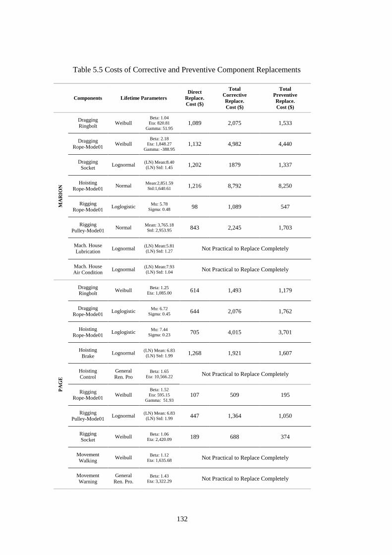
132

Table 5.5 Costs of Corrective and Preventive Component Replacements

Components Lifetime Parameters

Direct

Replace.

Cost ($)

Total

Corrective

Replace.

Cost ($)

Total

Preventive

Replace.

Cost ($)

MA

RIO

N

Dragging

Ringbolt Weibull

Beta: 1.04

Eta: 820.81

Gamma: 51.95 1,089 2,075 1,533

Dragging Rope-Mode01

Weibull Beta: 2.18

Eta: 1,848.27

Gamma: -388.95 1,132 4,982 4,440

Dragging Socket

Lognormal (LN) Mean:8.40

(LN) Std: 1.45 1,202 1879 1,337

Hoisting

Rope-Mode01 Normal

Mean:2,851.59

Std:1,640.61 1,216 8,792 8,250

Rigging

Rope-Mode01 Loglogistic

Mu: 5.78

Sigma: 0.48 98 1,089 547

Rigging

Pulley-Mode01 Normal

Mean: 3,765.18

Std: 2,953.95 843 2,245 1,703

Mach. House

Lubrication Lognormal

(LN) Mean:5.81

(LN) Std: 1.27 Not Practical to Replace Completely

Mach. House Air Condition

Lognormal (LN) Mean:7.93

(LN) Std: 1.04 Not Practical to Replace Completely

PA

GE

Dragging

Ringbolt Weibull

Beta: 1.25

Eta: 1,085.00 614 1,493 1,179

Dragging

Rope-Mode01 Loglogistic

Mu: 6.72

Sigma: 0.45 644 2,076 1,762

Hoisting

Rope-Mode01 Loglogistic

Mu: 7.44

Sigma: 0.23 705 4,015 3,701

Hoisting

Brake Lognormal

(LN) Mean: 6.83

(LN) Std: 1.99 1,268 1,921 1,607

Hoisting

Control

General

Ren. Pro Beta: 1.65

Eta: 10,566.22 Not Practical to Replace Completely

Rigging Rope-Mode01

Weibull Beta: 1.52

Eta: 595.15

Gamma: 51.93 107 509 195

Rigging Pulley-Mode01

Lognormal (LN) Mean: 6.83

(LN) Std: 1.99 447 1,364 1,050

Rigging

Socket Weibull

Beta: 1.06

Eta: 2,420.09 189 688 374

Movement

Walking Weibull

Beta: 1.12

Eta: 1,635.68 Not Practical to Replace Completely

Movement

Warning

General

Ren. Pro. Beta: 1.43

Eta: 3,322.29 Not Practical to Replace Completely

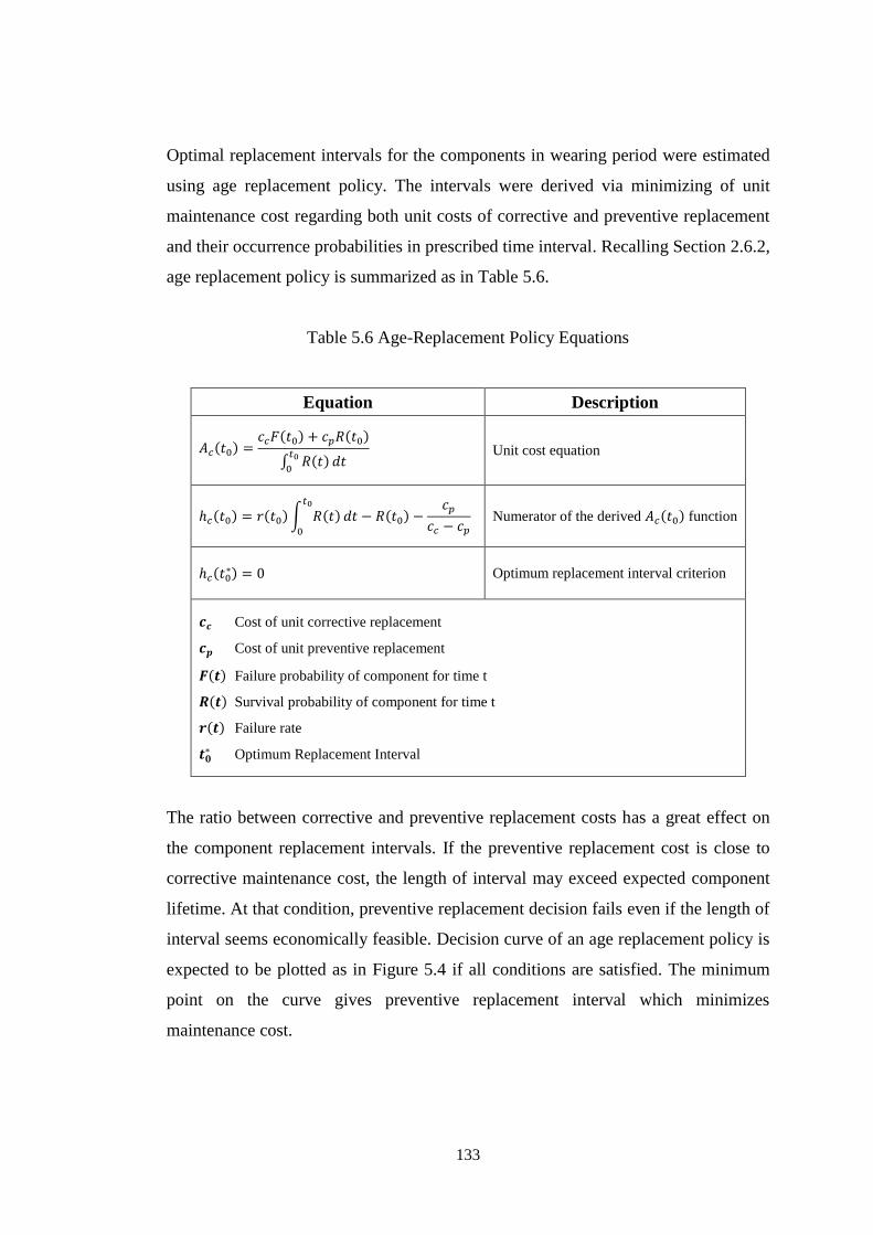
133

Optimal replacement intervals for the components in wearing period were estimated

using age replacement policy. The intervals were derived via minimizing of unit

maintenance cost regarding both unit costs of corrective and preventive replacement

and their occurrence probabilities in prescribed time interval. Recalling Section 2.6.2,

age replacement policy is summarized as in Table 5.6.

Table 5.6 Age-Replacement Policy Equations

Equation Description

𝐴𝑐(𝑡0) =𝑐𝑐𝐹(𝑡0) + 𝑐𝑝𝑅(𝑡0)

∫ 𝑅(𝑡)𝑡0

0𝑑𝑡

Unit cost equation

ℎ𝑐(𝑡0) = 𝑟(𝑡0) ∫ 𝑅(𝑡)𝑡0

0

𝑑𝑡 − 𝑅(𝑡0) −𝑐𝑝

𝑐𝑐 − 𝑐𝑝

Numerator of the derived 𝐴𝑐(𝑡0) function

ℎ𝑐(𝑡0∗) = 0 Optimum replacement interval criterion

𝒄𝒄 Cost of unit corrective replacement

𝒄𝒑 Cost of unit preventive replacement

𝑭(𝒕) Failure probability of component for time t

𝑹(𝒕) Survival probability of component for time t

𝒓(𝒕) Failure rate

𝒕𝟎∗ Optimum Replacement Interval

The ratio between corrective and preventive replacement costs has a great effect on

the component replacement intervals. If the preventive replacement cost is close to

corrective maintenance cost, the length of interval may exceed expected component

lifetime. At that condition, preventive replacement decision fails even if the length of

interval seems economically feasible. Decision curve of an age replacement policy is

expected to be plotted as in Figure 5.4 if all conditions are satisfied. The minimum

point on the curve gives preventive replacement interval which minimizes

maintenance cost.

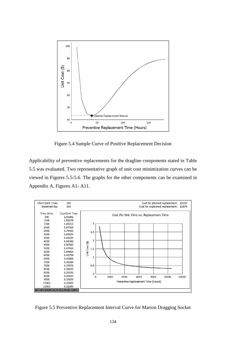
134

Figure 5.4 Sample Curve of Positive Replacement Decision

Applicability of preventive replacements for the dragline components stated in Table

5.5 was evaluated. Two representative graph of unit cost minimization curves can be

viewed in Figures 5.5-5.6. The graphs for the other components can be examined in

Appendix A, Figures A1- A11.

Figure 5.5 Preventive Replacement Interval Curve for Marion Dragging Socket

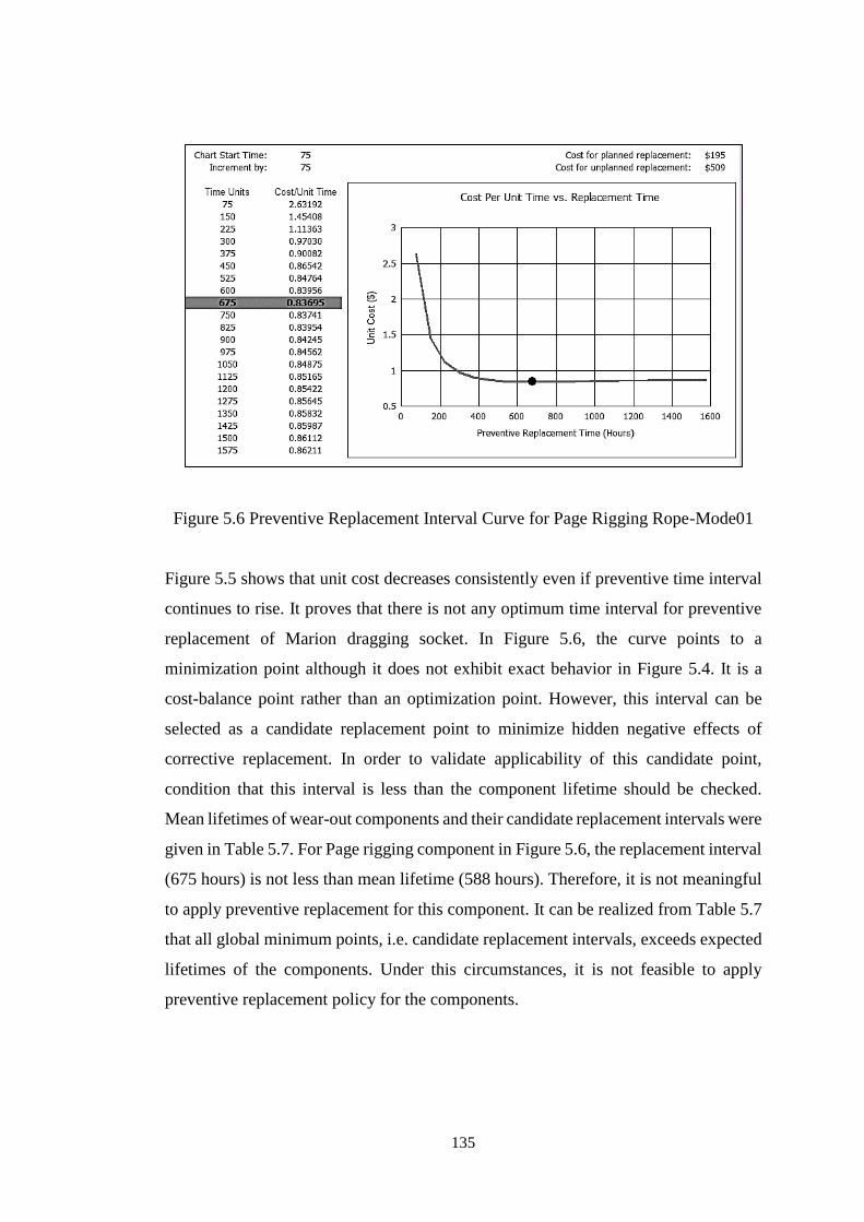
135

Figure 5.6 Preventive Replacement Interval Curve for Page Rigging Rope-Mode01

Figure 5.5 shows that unit cost decreases consistently even if preventive time interval

continues to rise. It proves that there is not any optimum time interval for preventive

replacement of Marion dragging socket. In Figure 5.6, the curve points to a

minimization point although it does not exhibit exact behavior in Figure 5.4. It is a

cost-balance point rather than an optimization point. However, this interval can be

selected as a candidate replacement point to minimize hidden negative effects of

corrective replacement. In order to validate applicability of this candidate point,

condition that this interval is less than the component lifetime should be checked.

Mean lifetimes of wear-out components and their candidate replacement intervals were

given in Table 5.7. For Page rigging component in Figure 5.6, the replacement interval

(675 hours) is not less than mean lifetime (588 hours). Therefore, it is not meaningful

to apply preventive replacement for this component. It can be realized from Table 5.7

that all global minimum points, i.e. candidate replacement intervals, exceeds expected

lifetimes of the components. Under this circumstances, it is not feasible to apply

preventive replacement policy for the components.

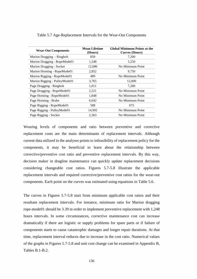
136

Table 5.7 Age-Replacement Intervals for the Wear-Out Components

Wear-Out Components Mean Lifetime

(Hours)

Global Minimum Points at the

Curves (Hours)

Marion Dragging - Ringbolt 859 7,200

Marion Dragging - RopeMode01 1,248 5,250

Marion Dragging - Socket 12,686 No Minimum Point

Marion Hoisting - RopeMode01 2,852 9,750

Marion Rigging - RopeMode01 489 No Minimum Point

Marion Rigging - PulleyMode01 3,765 12,000

Page Dragging - Ringbolt 1,011 7,200

Page Dragging - RopeMode01 2,521 No Minimum Point

Page Hoisting - RopeMode01 1,848 No Minimum Point

Page Hoisting - Brake 6,642 No Minimum Point

Page Rigging - RopeMode01 588 675

Page Rigging - PulleyMode01 14,902 No Minimum Point

Page Rigging - Socket 2,363 No Minimum Point

Wearing levels of components and ratio between preventive and corrective

replacement costs are the main determinants of replacement intervals. Although

current data utilized in the analyses points to infeasibility of replacement policy for the

components, it may be beneficial to learn about the relationship between

corrective/preventive cost ratio and preventive replacement intervals. By this way,

decision maker in dragline maintenance can quickly update replacement decisions

considering changeable cost ratios. Figures 5.7-5.8 illustrate the applicable

replacement intervals and required corrective/preventive cost ratios for the wear-out

components. Each point on the curves was estimated using equations in Table 5.6.

The curves in Figures 5.7-5.8 start from minimum applicable cost ratios and their

resultant replacement intervals. For instance, minimum ratio for Marion dragging

rope-mode01 should be 3.39 in order to implement preventive replacement with 1,248

hours intervals. In some circumstances, corrective maintenance cost can increase

dramatically if there are logistic or supply problems for spare parts or if failure of

components starts to cause catastrophic damages and longer repair durations. At that

time, replacement interval reduces due to increase in the cost ratio. Numerical values

of the graphs in Figures 5.7-5.8 and unit cost change can be examined in Appendix B,

Tables B.1-B.2.

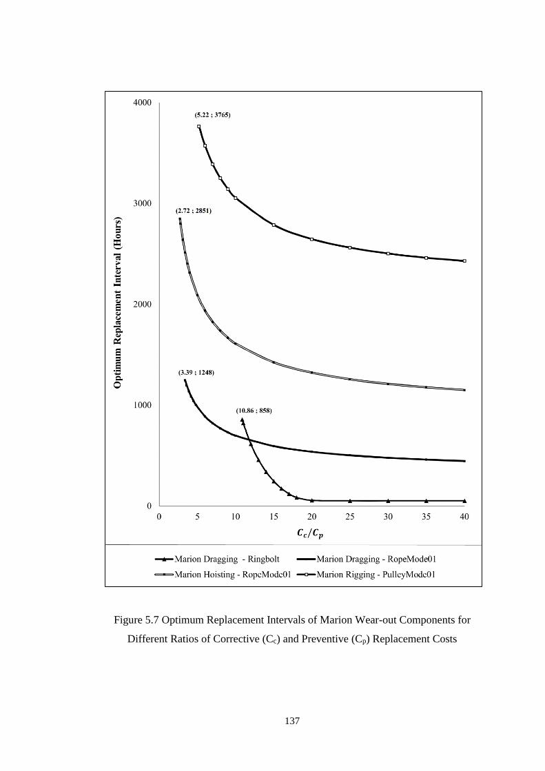
137

Figure 5.7 Optimum Replacement Intervals of Marion Wear-out Components for

Different Ratios of Corrective (Cc) and Preventive (Cp) Replacement Costs

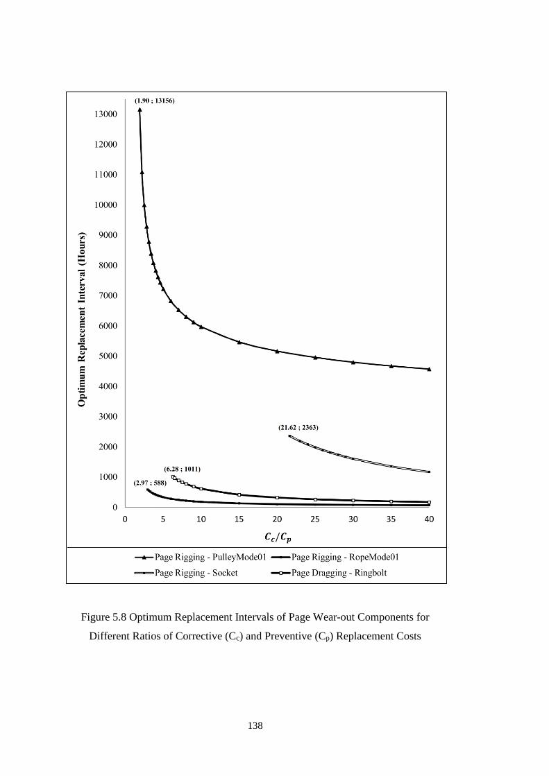
138

Figure 5.8 Optimum Replacement Intervals of Page Wear-out Components for

Different Ratios of Corrective (Cc) and Preventive (Cp) Replacement Costs

139

5.3.2 Development of an Optimization Algorithm for Inspection Intervals

Inspections are generally carried out at regular intervals to detect deficiencies in the

systems and to maintain components preventively against the potential failures. Scope

of an inspections is specified in advance and answers the questions of who, how, and

how long to perform the activities effectively during implementation period. In this

sense, the scope should specify i) components which should be concentrated on during

the period, ii) which strategy should be applied for correct maintenance decision of

individual components, and iii) the thresholds to initiate repairing or replacement

activities. Inspection works can be modified according to different operation

conditions and changing failure profiles of systems. Draglines in Tunçbilek coal mine

are inspected at 160 hours intervals with 8 hours durations. Common activities of

inspections for the draglines are listed as:

Dragging Unit

In case of wear-out in normal level, damaged zones on drag chains are welded. If

wear-out is in excessive level or irrecoverable fracture takes place on the

component, it is replaced with an identical one.

In case of wear-out in normal level, damaged zones on drag ringbolt are welded. If

wear-out is in excessive level or irrecoverable fracture takes place on the

component, it is replaced with an identical one. The component is also lubricated

against friction.

Tips of the drag ropes in the socket is controlled. If rope tips are scotched, these

parts are cut and fixed again with the ringbolt. Wire fractures and wear-out

condition are controlled along the whole rope. If there is ruptures on the

components, it is replaced with the identical one. This replacement can be out of

the regular inspection hours.

In drag control part, transmission boxes, gears, bearings, felts, lubrication leakages,

valves, brake linings, limit switches, hoist drums, hoist drum gears, and couplings

are controlled. If there is short-period repair requirement, this repair is carried out.

In case of long-time repairing requirement, a maintenance plan is developed with a

planned system shutdown.

140

Hoisting Unit

Tips of the hoist ropes in the socket is controlled. If rope tips are scotched, these

parts are cut and fixed again with the ringbolt. Wire fractures and wear-out

condition are controlled along the whole rope. If there is ruptures on the

components, it is replaced with the identical one. This replacement can be out of

the regular inspection hours.

In hoist control part, transmission boxes, gears, bearings, felts, lubrication leakages,

valves, brake linings, limit switches, hoist drums, hoist drum gears, and couplings

are controlled. If there is short-period repair requirement, this repair is carried out.

In case of long-time repairing requirement, a maintenance with a planned system

shutdown plan is developed.

Rigging Unit

Wire fractures and wear-outs on rigging rope and breaks, fractures and wear-out on

rigging sockets and rigging pulleys are controlled. Repair activities on these

components are not recommended. Instead, they are replaced with an identical ones

in case of any problem. In obligatory cases, some minor repairs can be performed

for these components.

Bucket Unit

Bucket teeth, chains, and ringbolts are repaired if required.

Some partial repairs can also be made on bucket main body. For general

maintenance of bucket, bucket body can be replaced with its spare without

interrupting dragline production.

Boom Unit

Welding of chord connections and condition of chords against buckling, fracture

and any other deficiencies are controlled. Maintenance on boom must be performed

with a scheduled and planned program.

Movement Unit

In rotation mechanism, gears of transmission box, bearings, felts, operating status

of lubrication pumps, lubrication leakages at the felts of main rotation axle, pinion

gears at the tips of main rotation axle, pulleys of turret traversing mechanism, rails,

flanges, and wear-out condition at any of these components are controlled. Failures

141

at this mechanism are repaired with a prescribed program or failed components are

replaced with an identical one.

In walking mechanism, gears of transmission box, bearings, felts, lubrication lines

and their injectors, walking axle, journal bearing, bushing of walking feet and their

pins, steel construction of walking feet are controlled against any deformation. The

anomalies that can be fixed in place are maintained with a planned program.

In warning mechanism, connection couplings, warning generator brushes, and

condition of whether there is any arc at armature or not are controlled. If the brushes

are eroded, they are replaced with a new one. Brush dust is removed with

compressed air against probability of dust to initiate any short circuit due to arc. If

any arc is initiated at armatures, these arc are removed via grinding armatures with

a portable grinding machine or turning lathe.

Machinery House

Generators are connected to each other with coupled sliding bearing system.

Coupling settings, wear-outs at the sliding bearing, and cleanness of liquid mineral

oil which maintain the bearings are controlled. Generator armature brushes and

occurrence condition of arc at the armatures are controlled. If the brushes are eroded

it is replaced with a new one. Brush dust is removed with compressed air against

probability of dust to initiate any short circuit due to arc. If any arc is initiated at

armatures, this arc are removed via grinding armatures with a portable grinding

machine or turning lathe. Electrical connections at generators are controlled.

Mechanical and electrical connections, armatures, brushes, bearings, and

lubrication feedings of all motors are controlled. If there is any failure that can be

recovered in-place, it is fixed. Critical failures are fixed at the workshop.

Lubrication requirement of dragline components are met with two type of automatic

lubrication systems. Injectors at lubrication line, valves, oil stock is the mechanism,

pumps, air compressors, valves of the air system, and timing mechanism are

controlled. The parts in malfunctioning state are repaired immediately.

Time between inspections, i.e. inspection intervals, highly effect annual maintenance

cost of draglines. If the interval is shortened too much in order to take more preventive

precautions, it causes halt of the machinery with high frequency. Therefore, production

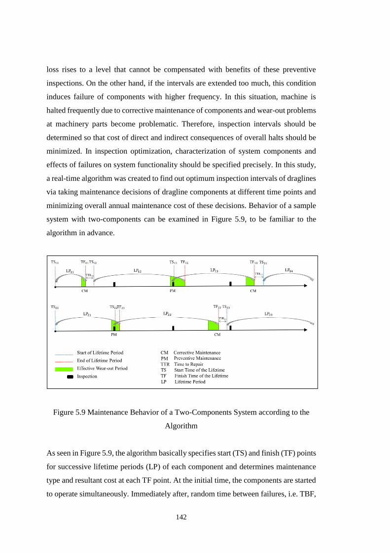
142

loss rises to a level that cannot be compensated with benefits of these preventive

inspections. On the other hand, if the intervals are extended too much, this condition

induces failure of components with higher frequency. In this situation, machine is

halted frequently due to corrective maintenance of components and wear-out problems

at machinery parts become problematic. Therefore, inspection intervals should be

determined so that cost of direct and indirect consequences of overall halts should be

minimized. In inspection optimization, characterization of system components and

effects of failures on system functionality should be specified precisely. In this study,

a real-time algorithm was created to find out optimum inspection intervals of draglines

via taking maintenance decisions of dragline components at different time points and

minimizing overall annual maintenance cost of these decisions. Behavior of a sample

system with two-components can be examined in Figure 5.9, to be familiar to the

algorithm in advance.

Figure 5.9 Maintenance Behavior of a Two-Components System according to the

Algorithm

As seen in Figure 5.9, the algorithm basically specifies start (TS) and finish (TF) points

for successive lifetime periods (LP) of each component and determines maintenance

type and resultant cost at each TF point. At the initial time, the components are started

to operate simultaneously. Immediately after, random time between failures, i.e. TBF,

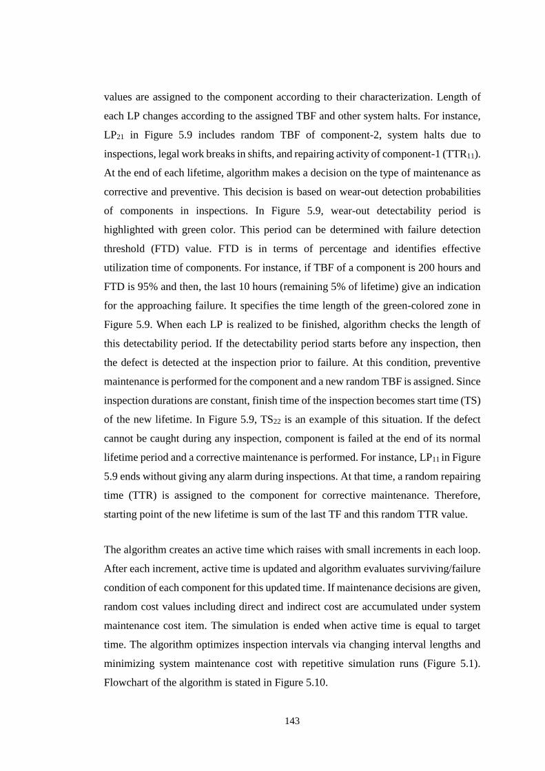
143

values are assigned to the component according to their characterization. Length of

each LP changes according to the assigned TBF and other system halts. For instance,

LP21 in Figure 5.9 includes random TBF of component-2, system halts due to

inspections, legal work breaks in shifts, and repairing activity of component-1 (TTR11).

At the end of each lifetime, algorithm makes a decision on the type of maintenance as

corrective and preventive. This decision is based on wear-out detection probabilities

of components in inspections. In Figure 5.9, wear-out detectability period is

highlighted with green color. This period can be determined with failure detection

threshold (FTD) value. FTD is in terms of percentage and identifies effective

utilization time of components. For instance, if TBF of a component is 200 hours and

FTD is 95% and then, the last 10 hours (remaining 5% of lifetime) give an indication

for the approaching failure. It specifies the time length of the green-colored zone in

Figure 5.9. When each LP is realized to be finished, algorithm checks the length of

this detectability period. If the detectability period starts before any inspection, then

the defect is detected at the inspection prior to failure. At this condition, preventive

maintenance is performed for the component and a new random TBF is assigned. Since

inspection durations are constant, finish time of the inspection becomes start time (TS)

of the new lifetime. In Figure 5.9, TS22 is an example of this situation. If the defect

cannot be caught during any inspection, component is failed at the end of its normal

lifetime period and a corrective maintenance is performed. For instance, LP11 in Figure

5.9 ends without giving any alarm during inspections. At that time, a random repairing

time (TTR) is assigned to the component for corrective maintenance. Therefore,

starting point of the new lifetime is sum of the last TF and this random TTR value.

The algorithm creates an active time which raises with small increments in each loop.

After each increment, active time is updated and algorithm evaluates surviving/failure

condition of each component for this updated time. If maintenance decisions are given,

random cost values including direct and indirect cost are accumulated under system

maintenance cost item. The simulation is ended when active time is equal to target

time. The algorithm optimizes inspection intervals via changing interval lengths and

minimizing system maintenance cost with repetitive simulation runs (Figure 5.1).

Flowchart of the algorithm is stated in Figure 5.10.

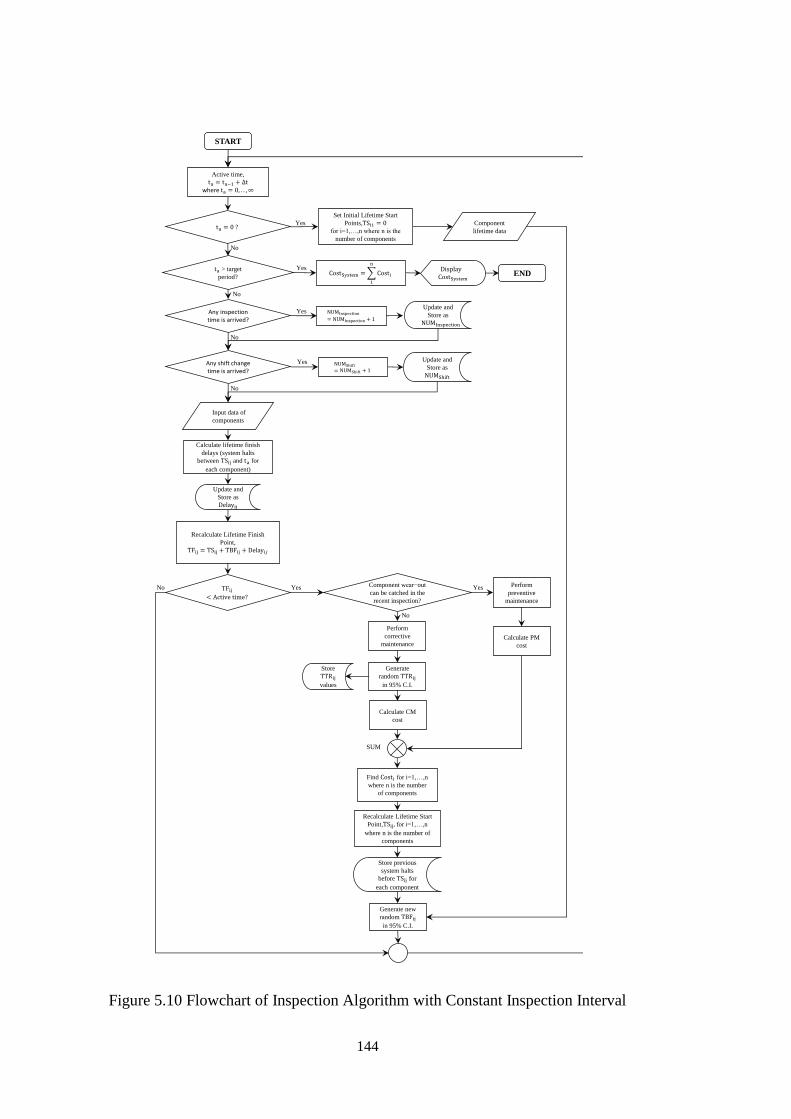
144

Active time,

where

Input data of

components

Any inspection time is arrived?

Any shift change time is arrived?

Recalculate Lifetime Finish

Point,

Component wear−out

can be catched in the

recent inspection?

Perform

preventive

maintenance

Perform

corrective

maintenance

Generate

random

in 95% C.I.

Calculate CM

cost

START

> target

period? END

Generate new

random

in 95% C.I.

Store

values

Yes

No

Yes

No

Yes

No

No Yes

Update and

Store as

Update and

Store as

Calculate PM

cost

Find for i=1,…,n

where n is the number

of components

SUM

Display

Recalculate Lifetime Start

Point, for i=1,…,n

where n is the number of

components

Store previous

system halts

before for

each component

Calculate lifetime finish

delays (system halts

between and for

each component)

Yes

No

Set Initial Lifetime Start

Points,

for i=1,…,n where n is the

number of components

Component

lifetime data

Update and

Store as

Yes

No

Figure 5.10 Flowchart of Inspection Algorithm with Constant Inspection Interval

145

Summary of algorithm stages and main assumptions can be investigated as follows:

Algorithm computes five dependent sub-events in each loop: Time counting,

estimation of lifetime period length, maintenance decision-making, assignment of

a start point for new lifetime, and cost estimation.

Time Counting:

Algorithm starts with t0=0. It increases with unit time increments and creates an

updated active times at the start of each loop.

When the updated active time reaches to any shift or inspection time, it counts and

updates the total number of shift or inspection from the beginning. By this way,

scheduled system halts are stored.

Estimation of Lifetime Period Lengths:

At t0=0, system components are initiated to operate simultaneously with random

survival times, i.e. TBF, according to their lifetime characteristics.

The algorithm estimates length of lifetime (LP) where component is operable via

assigning start (TS) and finish (TF) points to individual lifetimes. In addition to

component’s survival time, updated system halts due to inspections, shifts, and

corrective maintenance of other system components are also added to find out

updated TF points. This condition does not affect survival times of components,

only shifts TF points on the timeline.

Decision of Maintenance Type:

When active time arrives to TF of any component, the algorithm analyzes

probability of component wear-out to be detected at the previous inspection.

The algorithm assumes that the anomaly at component can be detected during this

inspection if wear-out period starts before the inspection. In this condition, a

preventive maintenance takes place for the component.

If there is a sudden or hidden failure for component without any indication or wear-

out period does not initiate before the previous inspection, the component is

assumed to be failed during operation and a corrective maintenance is performed.

Assignment of a Start Point for New Lifetime:

After each maintenance activity, a new random TBF is assigned to the maintained

component. Starting point of new lifetime is estimated with one of the following

assumptions: i) Summation of the last TF and random time-to-repair (TTR) value

146

after corrective maintenance or ii) finish time of the last inspection time after

preventive maintenance. TTR values for corrective maintenance are assigned

randomly considering repair time distributions of components.

Maintenance Cost Estimator:

Maintenance costs of individual components are stored as preventive and corrective

maintenance costs cumulatively. Since preventive maintenance takes place only in

regular inspections, production loss due to the maintenance is ignored in cost

estimation of preventive maintenance. In corrective maintenance, indirect cost is

estimated considering assigned random TTR in each activity. Corrective

maintenance cost is also determined randomly.

Maintenance cost of each component is accumulated in system maintenance cost

item until active time reached to the target analysis time and then simulation is

ended.

Overall maintenance cost of system is evaluated for changing inspection intervals

with repetitive simulation runs. The interval which minimizes the overall cost is

obtained as optimal interval.

The algorithm utilized following variables: i) Component lifetime characteristics, ii)

time-to-repair distributions of components, iii) failure detection thresholds (FTD), iv)

corrective costs of components in case of failures, v) preventive cost of components

when maintained in inspections, vi) unit production losses in system halts, and vii)

planned system halts during shifts and inspection. In the algorithm, random TBFs of

components was provided from lifetime characteristics obtained in Section 4.2.

Random repair durations (TTR) were assigned from distributions in Table 5.2. Failure

detection threshold (FTD) values were determined according to the opinions of

dragline maintenance experts (Table 5.8).Corrective costs after each failure covered

indirect and direct cost values. Constant direct cost values were taken from Table 5.3.

On the other hand, indirect cost values were designated randomly due to random TTR

values, using Equation 5.2. Preventive costs included only direct inspection costs of

components since inspections were carried out in constant durations. These values are

up-to-date values of year 2015 as given in Table 5.8. In addition, unit production losses

for both draglines were stated in Table 5.1. Planned system halts in each shift and

inspection were taken as 30 minutes and 8 hours, respectively.

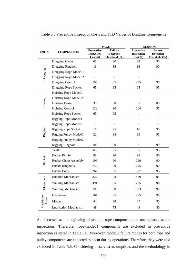
147

Table 5.8 Preventive Inspection Costs and FTD Values of Dragline Components

UNITS COMPONENTS

PAGE MARION

Preventive

Inspection

Cost ($)

Failure

Detection

Threshold (%)

Preventive

Inspection

Cost ($)

Failure

Detection

Threshold (%)

Dra

gg

ing

Dragging Chain 65 90 98 95

Dragging Ringbolt 16 85 16 90

Dragging Rope-Mode01 - - - -

Dragging Rope-Mode02 - - - -

Dragging Control 196 85 295 90

Dragging Rope Socket 65 95 65 95

Ho

isti

ng

Hoisting Rope-Mode01 - - - -

Hoisting Rope-Mode02 - - - -

Hoisting Brake 33 80 65 85

Hoisting Control 123 90 164 95

Hoisting Rope Socket 65 95 - -

Rig

gin

g

Rigging Rope-Mode01 - - - -

Rigging Rope-Mode02 - - - -

Rigging Rope Socket 16 95 16 95

Rigging Pulley-Mode01 22 98 33 95

Rigging Pulley-Mode02 - - - -

Rigging Ringbolt 109 90 131 90

Bu

cket

Teeth 65 95 65 95

Bucket Pin Set 98 90 98 90

Bucket Chain Assembly 196 90 229 90

Bucket Ringbolts 245 90 245 90

Bucket Body 262 95 327 95

Mo

vem

ent Rotation Mechanism 327 98 589 95

Walking Mechanism 491 95 785 90

Warning Mechanism 196 90 393 90

Mac

hin

ery

Ho

use

Generators 164 95 295 90

Motors 44 98 87 95

Lubrication Mechanism 49 75 49 80

As discussed at the beginning of section, rope components are not replaced at the

inspections. Therefore, rope-mode01 components are excluded in preventive

inspection as stated in Table 5.8. Moreover, mode02 failure modes for both rope and

pulley components are expected to occur during operations. Therefore, they were also

excluded in Table 5.8. Considering these cost assumptions and the methodology in

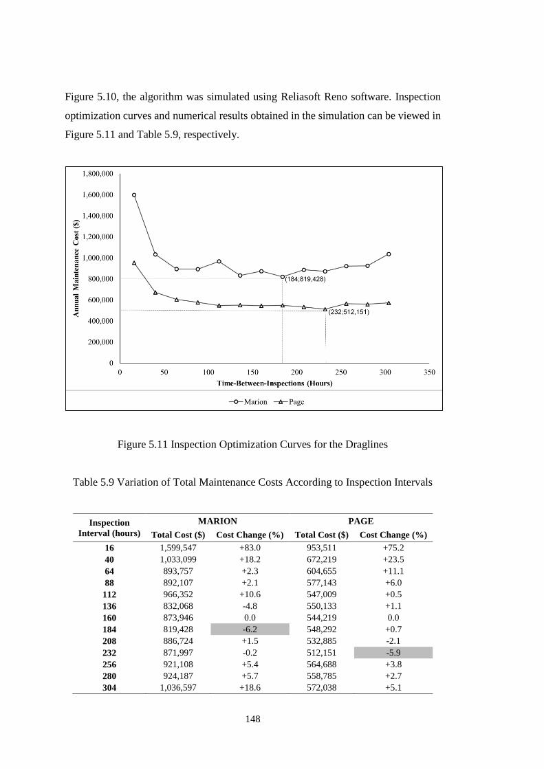
148

Figure 5.10, the algorithm was simulated using Reliasoft Reno software. Inspection

optimization curves and numerical results obtained in the simulation can be viewed in

Figure 5.11 and Table 5.9, respectively.

Figure 5.11 Inspection Optimization Curves for the Draglines

Table 5.9 Variation of Total Maintenance Costs According to Inspection Intervals

Inspection

Interval (hours)

MARION PAGE

Total Cost ($) Cost Change (%) Total Cost ($) Cost Change (%)

16 1,599,547 +83.0 953,511 +75.2

40 1,033,099 +18.2 672,219 +23.5

64 893,757 +2.3 604,655 +11.1

88 892,107 +2.1 577,143 +6.0

112 966,352 +10.6 547,009 +0.5

136 832,068 -4.8 550,133 +1.1

160 873,946 0.0 544,219 0.0

184 819,428 -6.2 548,292 +0.7

208 886,724 +1.5 532,885 -2.1

232 871,997 -0.2 512,151 -5.9

256 921,108 +5.4 564,688 +3.8

280 924,187 +5.7 558,785 +2.7

304 1,036,597 +18.6 572,038 +5.1

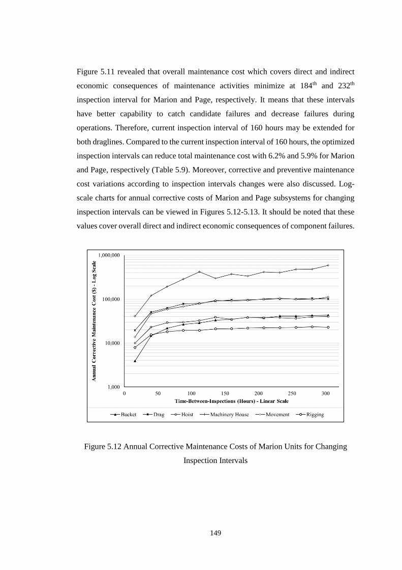
149

Figure 5.11 revealed that overall maintenance cost which covers direct and indirect

economic consequences of maintenance activities minimize at 184th and 232th

inspection interval for Marion and Page, respectively. It means that these intervals

have better capability to catch candidate failures and decrease failures during

operations. Therefore, current inspection interval of 160 hours may be extended for

both draglines. Compared to the current inspection interval of 160 hours, the optimized

inspection intervals can reduce total maintenance cost with 6.2% and 5.9% for Marion

and Page, respectively (Table 5.9). Moreover, corrective and preventive maintenance

cost variations according to inspection intervals changes were also discussed. Log-

scale charts for annual corrective costs of Marion and Page subsystems for changing

inspection intervals can be viewed in Figures 5.12-5.13. It should be noted that these

values cover overall direct and indirect economic consequences of component failures.

Figure 5.12 Annual Corrective Maintenance Costs of Marion Units for Changing

Inspection Intervals

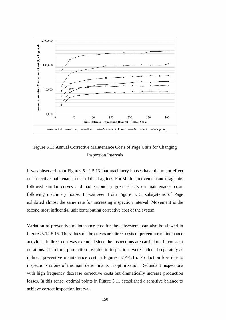
150

Figure 5.13 Annual Corrective Maintenance Costs of Page Units for Changing

Inspection Intervals

It was observed from Figures 5.12-5.13 that machinery houses have the major effect

on corrective maintenance costs of the draglines. For Marion, movement and drag units

followed similar curves and had secondary great effects on maintenance costs

following machinery house. It was seen from Figure 5.13, subsystems of Page

exhibited almost the same rate for increasing inspection interval. Movement is the

second most influential unit contributing corrective cost of the system.

Variation of preventive maintenance cost for the subsystems can also be viewed in

Figures 5.14-5.15. The values on the curves are direct costs of preventive maintenance

activities. Indirect cost was excluded since the inspections are carried out in constant

durations. Therefore, production loss due to inspections were included separately as

indirect preventive maintenance cost in Figures 5.14-5.15. Production loss due to

inspections is one of the main determinants in optimization. Redundant inspections

with high frequency decrease corrective costs but dramatically increase production

losses. In this sense, optimal points in Figure 5.11 established a sensitive balance to

achieve correct inspection interval.

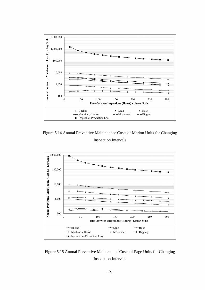
151

Figure 5.14 Annual Preventive Maintenance Costs of Marion Units for Changing

Inspection Intervals

Figure 5.15 Annual Preventive Maintenance Costs of Page Units for Changing

Inspection Intervals

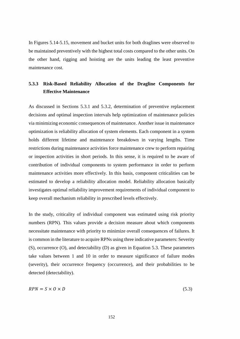
152

In Figures 5.14-5.15, movement and bucket units for both draglines were observed to

be maintained preventively with the highest total costs compared to the other units. On

the other hand, rigging and hoisting are the units leading the least preventive

maintenance cost.

5.3.3 Risk-Based Reliability Allocation of the Dragline Components for

Effective Maintenance

As discussed in Sections 5.3.1 and 5.3.2, determination of preventive replacement

decisions and optimal inspection intervals help optimization of maintenance policies

via minimizing economic consequences of maintenance. Another issue in maintenance

optimization is reliability allocation of system elements. Each component in a system

holds different lifetime and maintenance breakdown in varying lengths. Time

restrictions during maintenance activities force maintenance crew to perform repairing

or inspection activities in short periods. In this sense, it is required to be aware of

contribution of individual components to system performance in order to perform

maintenance activities more effectively. In this basis, component criticalities can be

estimated to develop a reliability allocation model. Reliability allocation basically

investigates optimal reliability improvement requirements of individual component to

keep overall mechanism reliability in prescribed levels effectively.

In the study, criticality of individual component was estimated using risk priority

numbers (RPN). This values provide a decision measure about which components

necessitate maintenance with priority to minimize overall consequences of failures. It

is common in the literature to acquire RPNs using three indicative parameters: Severity

(S), occurrence (O), and detectability (D) as given in Equation 5.3. These parameters

take values between 1 and 10 in order to measure significance of failure modes

(severity), their occurrence frequency (occurrence), and their probabilities to be

detected (detectability).

𝑅𝑃𝑁 = 𝑆 × 𝑂 × 𝐷 (5.3)

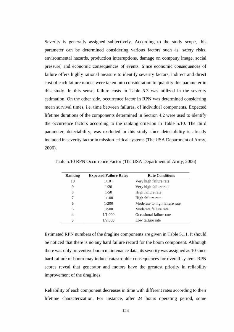
153

Severity is generally assigned subjectively. According to the study scope, this

parameter can be determined considering various factors such as, safety risks,

environmental hazards, production interruptions, damage on company image, social

pressure, and economic consequences of events. Since economic consequences of

failure offers highly rational measure to identify severity factors, indirect and direct

cost of each failure modes were taken into consideration to quantify this parameter in

this study. In this sense, failure costs in Table 5.3 was utilized in the severity

estimation. On the other side, occurrence factor in RPN was determined considering

mean survival times, i.e. time between failures, of individual components. Expected

lifetime durations of the components determined in Section 4.2 were used to identify

the occurrence factors according to the ranking criterion in Table 5.10. The third

parameter, detectability, was excluded in this study since detectability is already

included in severity factor in mission-critical systems (The USA Department of Army,

2006).

Table 5.10 RPN Occurrence Factor (The USA Department of Army, 2006)

Ranking Expected Failure Rates Rate Conditions

10 1/10+ Very high failure rate

9 1/20 Very high failure rate

8 1/50 High failure rate

7 1/100 High failure rate

6 1/200 Moderate to high failure rate

5 1/500 Moderate failure rate

4 1/1,000 Occasional failure rate

3 1/2,000 Low failure rate

Estimated RPN numbers of the dragline components are given in Table 5.11. It should

be noticed that there is no any hard failure record for the boom component. Although

there was only preventive boom maintenance data, its severity was assigned as 10 since

hard failure of boom may induce catastrophic consequences for overall system. RPN

scores reveal that generator and motors have the greatest priority in reliability

improvement of the draglines.

Reliability of each component decreases in time with different rates according to their

lifetime characterization. For instance, after 24 hours operating period, some

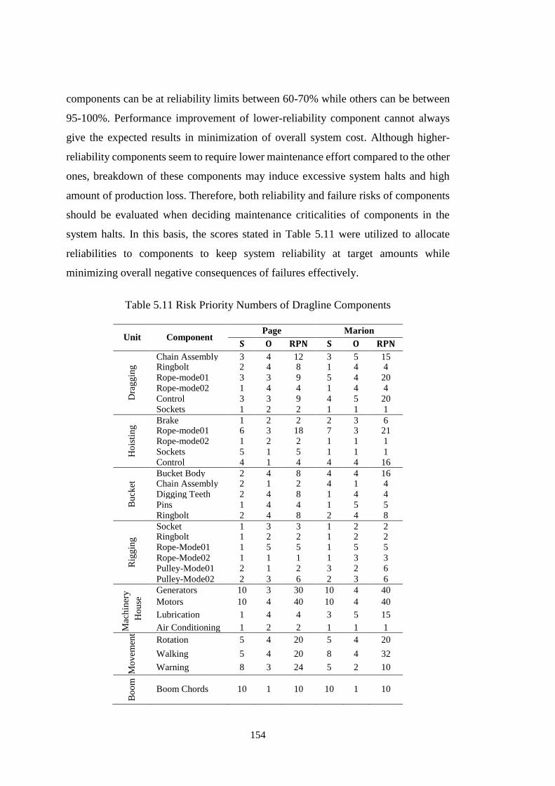
154

components can be at reliability limits between 60-70% while others can be between

95-100%. Performance improvement of lower-reliability component cannot always

give the expected results in minimization of overall system cost. Although higher-

reliability components seem to require lower maintenance effort compared to the other

ones, breakdown of these components may induce excessive system halts and high

amount of production loss. Therefore, both reliability and failure risks of components

should be evaluated when deciding maintenance criticalities of components in the

system halts. In this basis, the scores stated in Table 5.11 were utilized to allocate

reliabilities to components to keep system reliability at target amounts while

minimizing overall negative consequences of failures effectively.

Table 5.11 Risk Priority Numbers of Dragline Components

Unit Component Page Marion

𝐒 𝐎 𝐑𝐏𝐍 𝐒 𝐎 𝐑𝐏𝐍

Dra

gg

ing

Chain Assembly 3 4 12 3 5 15 Ringbolt 2 4 8 1 4 4

Rope-mode01 3 3 9 5 4 20 Rope-mode02 1 4 4 1 4 4

Control 3 3 9 4 5 20 Sockets 1 2 2 1 1 1

Ho

isti

ng

Brake 1 2 2 2 3 6 Rope-mode01 6 3 18 7 3 21 Rope-mode02 1 2 2 1 1 1

Sockets 5 1 5 1 1 1 Control 4 1 4 4 4 16

Bu

cket

Bucket Body 2 4 8 4 4 16 Chain Assembly 2 1 2 4 1 4 Digging Teeth 2 4 8 1 4 4

Pins 1 4 4 1 5 5 Ringbolt 2 4 8 2 4 8

Rig

gin

g

Socket 1 3 3 1 2 2 Ringbolt 1 2 2 1 2 2 Rope-Mode01 1 5 5 1 5 5

Rope-Mode02 1 1 1 1 3 3 Pulley-Mode01 2 1 2 3 2 6

Pulley-Mode02 2 3 6 2 3 6

Mac

hin

ery

Ho

use

Generators 10 3 30 10 4 40

Motors 10 4 40 10 4 40

Lubrication 1 4 4 3 5 15

Air Conditioning 1 2 2 1 1 1

Mo

vem

ent

Rotation 5 4 20 5 4 20

Walking 5 4 20 8 4 32

Warning 8 3 24 5 2 10

Bo

om

Boom Chords 10 1 10 10 1 10

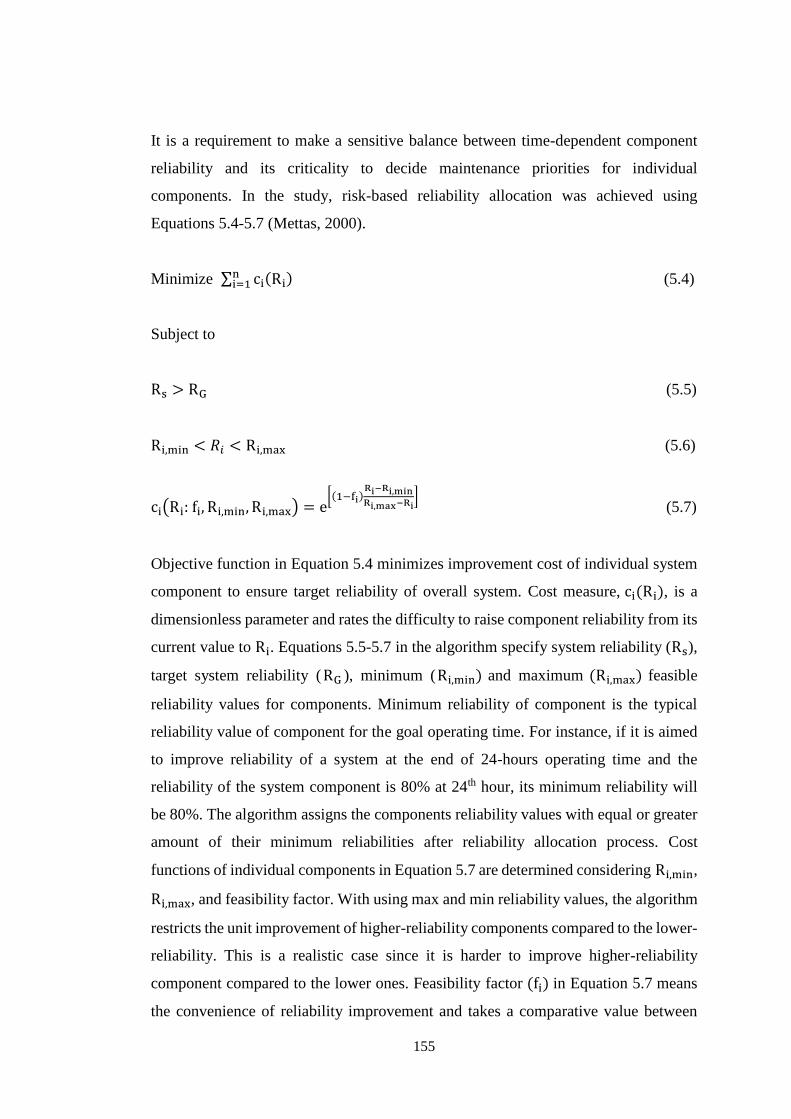
155

It is a requirement to make a sensitive balance between time-dependent component

reliability and its criticality to decide maintenance priorities for individual

components. In the study, risk-based reliability allocation was achieved using

Equations 5.4-5.7 (Mettas, 2000).

Minimize ∑ ci(Ri)ni=1 (5.4)

Subject to

Rs > RG (5.5)

Ri,min < 𝑅𝑖 < Ri,max (5.6)

ci(Ri: fi, Ri,min, Ri,max) = e[(1−fi)

Ri−Ri,minRi,max−Ri

] (5.7)

Objective function in Equation 5.4 minimizes improvement cost of individual system

component to ensure target reliability of overall system. Cost measure, ci(Ri), is a

dimensionless parameter and rates the difficulty to raise component reliability from its

current value to Ri. Equations 5.5-5.7 in the algorithm specify system reliability (Rs),

target system reliability (RG ), minimum (Ri,min) and maximum (Ri,max ) feasible

reliability values for components. Minimum reliability of component is the typical

reliability value of component for the goal operating time. For instance, if it is aimed

to improve reliability of a system at the end of 24-hours operating time and the

reliability of the system component is 80% at 24th hour, its minimum reliability will

be 80%. The algorithm assigns the components reliability values with equal or greater

amount of their minimum reliabilities after reliability allocation process. Cost

functions of individual components in Equation 5.7 are determined considering Ri,min,

Ri,max , and feasibility factor. With using max and min reliability values, the algorithm

restricts the unit improvement of higher-reliability components compared to the lower-

reliability. This is a realistic case since it is harder to improve higher-reliability

component compared to the lower ones. Feasibility factor (fi) in Equation 5.7 means

the convenience of reliability improvement and takes a comparative value between

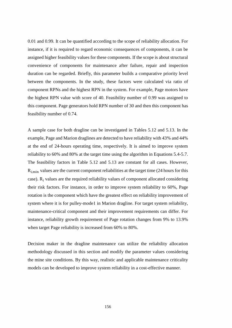
156

0.01 and 0.99. It can be quantified according to the scope of reliability allocation. For

instance, if it is required to regard economic consequences of components, it can be

assigned higher feasibility values for these components. If the scope is about structural

convenience of components for maintenance after failure, repair and inspection

duration can be regarded. Briefly, this parameter builds a comparative priority level

between the components. In the study, these factors were calculated via ratio of

component RPNs and the highest RPN in the system. For example, Page motors have

the highest RPN value with score of 40. Feasibility number of 0.99 was assigned to

this component. Page generators hold RPN number of 30 and then this component has

feasibility number of 0.74.

A sample case for both dragline can be investigated in Tables 5.12 and 5.13. In the

example, Page and Marion draglines are detected to have reliability with 43% and 44%

at the end of 24-hours operating time, respectively. It is aimed to improve system

reliability to 60% and 80% at the target time using the algorithm in Equations 5.4-5.7.

The feasibility factors in Table 5.12 and 5.13 are constant for all cases. However,

Ri,min values are the current component reliabilities at the target time (24 hours for this

case). Ri values are the required reliability values of component allocated considering

their risk factors. For instance, in order to improve system reliability to 60%, Page

rotation is the component which have the greatest effect on reliability improvement of

system where it is for pulley-mode1 in Marion dragline. For target system reliability,

maintenance-critical component and their improvement requirements can differ. For

instance, reliability growth requirement of Page rotation changes from 9% to 13.9%

when target Page reliability is increased from 60% to 80%.

Decision maker in the dragline maintenance can utilize the reliability allocation

methodology discussed in this section and modify the parameter values considering

the mine site conditions. By this way, realistic and applicable maintenance criticality

models can be developed to improve system reliability in a cost-effective manner.

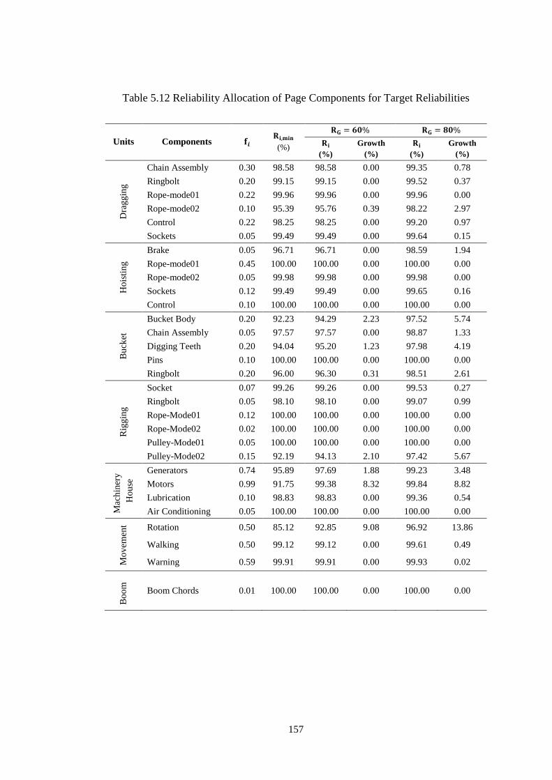
157

Table 5.12 Reliability Allocation of Page Components for Target Reliabilities

Units Components 𝐟𝒊 𝐑𝐢,𝐦𝐢𝐧

(%)

𝐑𝐆 = 𝟔𝟎% 𝐑𝐆 = 𝟖𝟎%

𝐑𝐢

(%)

Growth

(%)

𝐑𝐢

(%)

Growth

(%)

Dra

gg

ing

Chain Assembly 0.30 98.58 98.58 0.00 99.35 0.78

Ringbolt 0.20 99.15 99.15 0.00 99.52 0.37

Rope-mode01 0.22 99.96 99.96 0.00 99.96 0.00

Rope-mode02 0.10 95.39 95.76 0.39 98.22 2.97

Control 0.22 98.25 98.25 0.00 99.20 0.97

Sockets 0.05 99.49 99.49 0.00 99.64 0.15

Ho

isti

ng

Brake 0.05 96.71 96.71 0.00 98.59 1.94

Rope-mode01 0.45 100.00 100.00 0.00 100.00 0.00

Rope-mode02 0.05 99.98 99.98 0.00 99.98 0.00

Sockets 0.12 99.49 99.49 0.00 99.65 0.16

Control 0.10 100.00 100.00 0.00 100.00 0.00

Bu

cket

Bucket Body 0.20 92.23 94.29 2.23 97.52 5.74

Chain Assembly 0.05 97.57 97.57 0.00 98.87 1.33

Digging Teeth 0.20 94.04 95.20 1.23 97.98 4.19

Pins 0.10 100.00 100.00 0.00 100.00 0.00

Ringbolt 0.20 96.00 96.30 0.31 98.51 2.61

Rig

gin

g

Socket 0.07 99.26 99.26 0.00 99.53 0.27

Ringbolt 0.05 98.10 98.10 0.00 99.07 0.99

Rope-Mode01 0.12 100.00 100.00 0.00 100.00 0.00

Rope-Mode02 0.02 100.00 100.00 0.00 100.00 0.00

Pulley-Mode01 0.05 100.00 100.00 0.00 100.00 0.00

Pulley-Mode02 0.15 92.19 94.13 2.10 97.42 5.67

Mac

hin

ery

Ho

use

Generators 0.74 95.89 97.69 1.88 99.23 3.48

Motors 0.99 91.75 99.38 8.32 99.84 8.82

Lubrication 0.10 98.83 98.83 0.00 99.36 0.54

Air Conditioning 0.05 100.00 100.00 0.00 100.00 0.00

Mo

vem

ent Rotation 0.50 85.12 92.85 9.08 96.92 13.86

Walking 0.50 99.12 99.12 0.00 99.61 0.49

Warning 0.59 99.91 99.91 0.00 99.93 0.02

Bo

om

Boom Chords 0.01 100.00 100.00 0.00 100.00 0.00

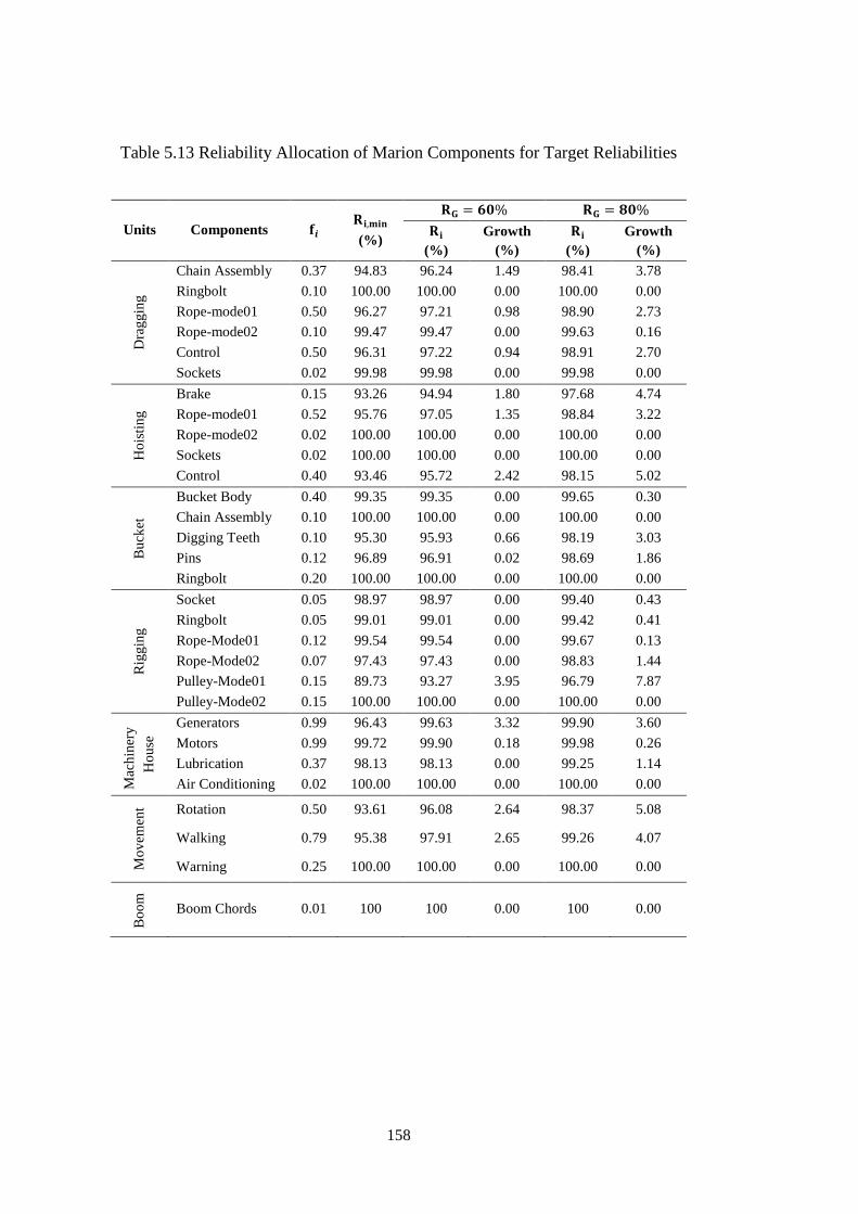
158

Table 5.13 Reliability Allocation of Marion Components for Target Reliabilities

Units Components 𝐟𝒊 𝐑𝐢,𝐦𝐢𝐧

(%)

𝐑𝐆 = 𝟔𝟎% 𝐑𝐆 = 𝟖𝟎%

𝐑𝐢

(%)

Growth

(%)

𝐑𝐢

(%)

Growth

(%)

Dra

gg

ing

Chain Assembly 0.37 94.83 96.24 1.49 98.41 3.78

Ringbolt 0.10 100.00 100.00 0.00 100.00 0.00

Rope-mode01 0.50 96.27 97.21 0.98 98.90 2.73

Rope-mode02 0.10 99.47 99.47 0.00 99.63 0.16

Control 0.50 96.31 97.22 0.94 98.91 2.70

Sockets 0.02 99.98 99.98 0.00 99.98 0.00

Ho

isti

ng

Brake 0.15 93.26 94.94 1.80 97.68 4.74

Rope-mode01 0.52 95.76 97.05 1.35 98.84 3.22

Rope-mode02 0.02 100.00 100.00 0.00 100.00 0.00

Sockets 0.02 100.00 100.00 0.00 100.00 0.00

Control 0.40 93.46 95.72 2.42 98.15 5.02

Bu

cket

Bucket Body 0.40 99.35 99.35 0.00 99.65 0.30

Chain Assembly 0.10 100.00 100.00 0.00 100.00 0.00

Digging Teeth 0.10 95.30 95.93 0.66 98.19 3.03

Pins 0.12 96.89 96.91 0.02 98.69 1.86

Ringbolt 0.20 100.00 100.00 0.00 100.00 0.00

Rig

gin

g

Socket 0.05 98.97 98.97 0.00 99.40 0.43

Ringbolt 0.05 99.01 99.01 0.00 99.42 0.41

Rope-Mode01 0.12 99.54 99.54 0.00 99.67 0.13

Rope-Mode02 0.07 97.43 97.43 0.00 98.83 1.44

Pulley-Mode01 0.15 89.73 93.27 3.95 96.79 7.87

Pulley-Mode02 0.15 100.00 100.00 0.00 100.00 0.00

Mac

hin

ery

Ho

use

Generators 0.99 96.43 99.63 3.32 99.90 3.60

Motors 0.99 99.72 99.90 0.18 99.98 0.26

Lubrication 0.37 98.13 98.13 0.00 99.25 1.14

Air Conditioning 0.02 100.00 100.00 0.00 100.00 0.00

Mo

vem

ent Rotation 0.50 93.61 96.08 2.64 98.37 5.08

Walking 0.79 95.38 97.91 2.65 99.26 4.07

Warning 0.25 100.00 100.00 0.00 100.00 0.00

Bo

om

Boom Chords 0.01 100 100 0.00 100 0.00

159

6. CONCLUSIONS AND RECOMMENDATIONS

6.1 Conclusions

Dragline is a massive earthmover that performs overburden stripping by itself via

successive cycles of dragging and hoisting bucket, swinging machinery house to spoil

area and dumping full bucket. Operational status of draglines raises the importance of

performance awareness for individual components in the mechanism. This situation

requires deductive evaluation of component characterization and understanding of

component effects on system performance. Underestimating root-causes of system

halts and preventive measures in maintenance policies can induce rapid degradation of

system elements and frequent system breakdowns. Draglines may suffer from

insufficient and poor maintenance policies which may reduce stripping productivity.

In this sense, sustainability of dragline operations can be improved via developing of

reliability-based maintenance optimization methods.

This study integrated system reliability modelling and maintenance optimization in

order to generate optimal maintenance policies for draglines. Using machinery

catalogues, expert opinions, and information in datasets, dragline system was

decomposed into subsystems and components considering functional and structural

dependencies in the system. Various statistical and graphical methods were used to

analyze behavior of individual datasets of components and to validate goodness of

data. Reliability modelling of subsystems were generated using the lifetime datasets

of components. Understanding of subsystem behavior allowed constitution of overall

system reliability model. In reliability analyses, failure modes of each component and

frequent maintenance strategy on them were also examined in detail. Evaluation of

time-varying component reliability and root-causes of system halts provided a basis to

criticize and build up maintenance optimization criteria for the draglines. In the study,

160

maintenance optimization issue was handled considering i) applicability of preventive

component replacements, ii) cost-effective inspection interval optimization, and iii)

risk-based reliability allocation of the components.

Following key conclusions can be drawn from this research study:

Data values for individual component should be checked for data anomalies such

as, clustering, oscillation, mixture, and trend. Any unexpected data gathering or

fluctuation can be indicator of deficiency in data collection or missing data. Run

charts offer useful analysis to detect potential data anomalies and their causes. In

addition, potential outlier values should also be controlled considering their

distribution characteristics. Although box plots can be utilized as a non-parametric

method, they can induce misleading inference for heavily-tailed distributions.

Therefore, decision on outliers can be made subjectively also regarding box plots

and distribution shape.

Although Crow-AMSAA is highly robust test, trend decisions on this type of

datasets should be interpreted using both qualitative and other quantitative methods.

Results of quantitative test can differs where hypothesis testing values are slightly

above or below the limit values. In this case, interpretation of data behavior

subjectively via considering recent periods instead of whole observation period can

be beneficial in trend decisions.

Reliability evaluation using reliability block diagrams analyzes the root-causes for

system failures effectively. Deductive structure of the method allows to investigate

contribution of individual components on system performance and to detect

weakest links in system productivity.

Extending/shortening lifetime duration points to lifetime trend and this condition

can be detected using trend tests. Reliability of this type of components is required

to be estimated using stochastic model which can measure lifetime

deterioration/growth. General Renewal Process is a flexible and effective method

to characterize trend-component in any level between as good as new and as bad as

old. Hoisting rope-mode02, hoisting control, bucket main body, bucket teeth,

bucket ringbolt, rigging pulley-mode02, generators, motors, rotation, and warning

161

mechanisms for Page dragline, dragging chain, hoisting brake, rigging socket, and

rotation mechanisms for Marion dragline were processed using General Renewal

Process. Reliability of other non-repairable and also non-trend repairable

components were estimated using best-fit distributions. Especially, Weibull

distribution was best-fitted in majority of the components.

Reliability assessment without analyzing failure modes and their maintenance types

can cause misinformation about the resultant reliability values. Common failure

modes and their repair activities were listed in the study to clear how reliability

improvement could be provided with which maintenance activities. Dragging,

hoisting, and rigging ropes are non-repairable components which fails due to

rupture and maintained with replacement. Although some other components such

as, chain, socket, and teeth are generally non-repairable, they are individual

members of the sets. Therefore, they were assumed as repairable mechanisms with

non-repairable subcomponents. Replacement of individual parts and welding are

common maintenance activities for the mechanical repairable components of

dragline. On the other hand, more complicated mechanisms, such as, motor,

generator, rotation, walking are maintained via repairing failed electrical and

mechanical subcomponents and also lubrication activities.

Resultant reliability values revealed that dragging and bucket subsystems have the

shortest lifetimes. Dragging unit is expected to survive for 210 and 170 hours for

Page and Marion draglines, respectively. It is 188 and 200 hours for the bucket

units. Boom is the least breakdown inducing unit for both draglines. Any failure in

this unit causes catastrophic failure and leads to long-period system halts. The

records on boom is only about preventive welding against fractures. Expected

intervals for preventive welding requirement of booms are 7,391 and 11,502 hours

for Page and Marion draglines, respectively. Reliability of overall system showed

that Page and Marion are expected to operate continuously for 35.6 and 34.0 hours,

respectively.

Although maintenance studies in the literature have generally considered

availability or reliability factors alone in optimization process, cost is the main

factor to develop more realistic and applicable policies. Availability factor can also

be included in cost parameter via considering economic consequences of

162

downtimes. This study evaluates cost of individual failure modes combining direct

and indirect cost values. Direct cost is the expected physical value of failure

consequences where indirect cost is production loss of downtimes. Estimation of

indirect cost is very important since indirect cost generally overtakes direct cost in

production industries. Unit production cost in the study for Marion and Page was

calculated as 9.03 and 5.23 $/min, respectively. It regarded the unit time revenue

from overburden excavation considering swell and fill factors, cycle time, bucket

capacity, and operator efficiency. On the other hand, direct costs are specific to the

components, obtained via questionnaires filled by dragline maintenance experts.

Regarding repair costs and production losses, motors and generators are expected

to induce the most destructive failure consequences, since their repair times are

comparatively larger than other components. On the other hand, mechanical

components such as, socket, teeth, ringbolt, and pin are generally recovered in

shorter periods and then they are expected to induce less economic consequences

in each failure.

The study used age-replacement policy to detect applicability of preventive

replacements for wear-out components. Dragging ringbolt, dragging rope-mode01,

dragging socket, hoisting rope-mode01, rigging rope-mode01, and rigging pulley-

mode01 for Marion dragline and dragging ringbolt, dragging rope-mode01, hoisting

rope-mode01, hoisting brake, rigging rope-mode01, rigging pulley-mode01,

rigging socket for Page dragline were determined as candidate wear-out

components for preventive replacement. Using age replacement equations, it was

decided that there is no applicability of age-replacements for the components in

current conditions. However, replacement interval graphs were plotted to evaluate

and update the decisions according to changeable ratios between corrective and

preventive replacement costs.

Risk analysis showed that machinery house and movement units are the subsystems

with the highest failure risk. Reliability allocation algorithm using risk factors

revealed that improvements in rotation and motor components offer the highest

contribution on dragline reliability in economical manner.

An original time counter algorithm was generated to obtain optimum inspection

intervals for draglines. The algorithm aimed to minimize overall annual

163

maintenance costs of draglines via changing inspection intervals. Random lifetime

behavior of all components, contributions of random failures and scheduled breaks

to system halts, and decisions on preventive/corrective maintenance for the

components were included in the algorithm. Cost values in maintenance decisions

of individual components were estimated randomly due to changing production

losses. The simulation showed that 184 and 232 hours intervals are optimal to carry

out inspections for Page and Marion, respectively. These optimal values are

expected to yield an economic savings with 6.2% for Page and 5.9% for Marion

compared to current inspection conditions at the mine site.

Maintenance and reliability assessment methodologies in the study and the

developed algorithm for inspection interval optimization offer an holistic view on

maintenance evaluation of all machinery systems as well as draglines. Decision

makers can utilize these methodologies to discuss maintenance and operational

performances of their systems.

6.2 Recommendations

Although the study is expected to make significant contribution to development of

maintenance strategies for draglines, various areas can be improved in future studies.

Recommendations on these areas are given as follows:

For healthy and detailed analysis of draglines, standards on maintenance recording

can be established and utilized at mine sites. A training can also be performed for

maintenance crew about how to standardize maintenance recording. Detailed

expression on causes and results of failures, statistics about required crew number

per failure, and detectability (delay time) condition before failures can be asked in

maintenance sheets. Failed components, existing failure modes, and repairing types

can be expressed using unique codes.

Constitution of a web-based maintenance platform for mining industry can be

beneficial for academic and industrial evaluation of maintenance efficiency for

mining machineries.

164

Dynamic maintenance policies can be developed regarding inflation rate,

production rate considering demand/supply amounts, changes in ore prices,

operator efficiency, effectiveness of maintenance crew, and convenience of weather

conditions for operations.

Spare part optimization is a challenging issue in maintenance optimization.

Reliability-based stock and demand plan for spare parts can be studied for mining

machineries as a future study.

Opportunistic maintenance and crew number optimization can be included in

maintenance policies of mining machineries.

There is not any record on delay-time maintenance of mining machinery component

for preventive replacement policies. A long-period maintenance recording plan can

be formed in mine sites to identify failure-alert periods of individual components.

According to failure modes, various field test can be applied to detect wear-out

rates.

Studies on inspection optimization generally aims to find out inspection intervals.

However, optimality of inspection duration is underestimated. Therefore, efficient

implementation duration for planned regular inspections can be detected

considering work packages in each inspection.

165

REFERENCES

Afefy, I. H. (2010). Reliability-Centered Maintenance Methodology and Application:

A Case Study. Engineering, 2(11), 863-873.

Aggarwal, K. K. (1993). Reliability Engineering. Dordrecht, The Netherlands: Kluwer

Academic Publishers.

Assaf, D. and Shanthikumar, J. G. (1987). Optimal Group Maintenance Policies With

Continuous and Periodic Inspections. Management Science, 33, 1440-1450.

Barabady, J. and Kumar, U. (2008). Reliability Analysis of Mining Equipment: A Case

Study of a Crushing Plant at Jajarm Bauxite Mine in Iran. Reliability

Engineering and System Safety, 647–653.

Barlow, R. E. and Hunter, L. C. (1960). Optimum Preventive Maintenance Policies.

Operations Research, 8, 90-100.

Barlow, R. E. and Proschan, F. (1965). Mathematical Theory of Reliability. New York:

John Wiley and Sons Ltd.

Ben-Daya, M., Duffuaa, S. O., and Raouf, A. (2000). Maintenance, Modeling and

Optimization. New York: Kluwer Academic Publishers.

Ben-Daya, M., Duffuaa, S. O., Raouf, A., Knezevic, J., and Ait-Kadi, D. (2009).

Handbook of Maintenance Management and Engineering. Springer-Verlag

London Limited.

Berg, M. and Epstein, B. (1976). A Modified Block Replacement Policy. Naval

Research Logistics, 23, 15-24.

Berk, J. (2009). Systems Failure Analysis. ASM International.

Bertsche, B. (2008). Reliability in Automotive and Mechnical Engineering. Springer-

Verlag Berlin Heidelberg.

Blischke, W. R. and Murthy, D. P. (2000). Reliability Modeling, Prediction, and

Optimization. Canada: John Wiley and Sons, Inc.

166

Block, H. W., Borges, W. S., and Savits, T. H. (1985). Age Dependent Minimal

Repair. Journal of Applied Probability, 22, 370-385.

Block, H. W., Borges, W. S., and Savits, T. H. (1988). A General Age Replacement

Model with Minimal Repair. Naval Research Logistics, 35(5), 365-372.

Block, H., Langberg, N., and Savits, T. (1993). Repair Replacement Policies. Journal

of Applied Probability, 30(1), 194–206.

Brown, M. and Proschan, F. (1983). Imperfect Repair. Journal of Appliaed

Probability, 20, 851-859.

Budai, G., Dekker, R., and Nicolai, R. P. (2008). Maintenance and Production: A

Review of Planning Models. In K. A. Kobbacy, and D. P. Murthy, Complex

System Maintenance handbook (pp. 321-344). Springer-Verlag London

Limited.

Cerone, P. (1991). On a Simplified Delay-Time Model of Reliability of Equipment

Subject to Inspection Monitoring. Journal of Operational Research Society,

42, 505-511.

Christer, A. H. (1976). Innovative Decision Making. NATO Conference on the Role of

Effectiveness of Theory of Decision in Practice, (pp. 368-377).

Christer, A. H. (1987). Delay-Time Models of Reliability of Equipment Subject to

Inspection Monitoring. The Journal of Operational Research Society, 38, 329-

334.

Christer, A. H. (1999). Developments in Delay Time Analysis for Modelling Plant

Maintenance. The Journal of the Operational Research Society, 50(11), 1120-

1137.

Christer, A. H. and Waller , W. M. (1984). Delay time Models of Industrial Inspection

Maintenance Problems. The Journal of the Operational Research Society, 35,

401-406.

Christer, A. H., Wang, W., and Lee, C. (2000). A Data Deficiency Based Parameter

Estimating Problem and Case Study in Delay Time PM Modelling. The

International Journal of Production Economics, 67(1), 63-76.

167

Christer, A. H., Wang, W., Baker, R. D., and Sharp, J. M. (1995). Modelling

Maintenance Practice of Production Plant Using the Delay Time Concept. IMA

Journal of Mathematics Applied in Business and Industry, 6, 67-83.

Christer, A. H., Wang, W., Sharp, J. M., and Baker, R. D. (1998). A Case Study of

Modelling Preventive Maintenance of Production Plant Using Subjective Data.

The Journal of the Operational Research Society, 49, 210-219.

Clark, D. (1990). Tribology – Its Applications to Equipment Reliability and

Maintainability Design in the Underground Coal Mining Industry. Proceedings

of the Institution of Engineers Aus- tralia Tribology Conference, (pp. 38-44).

Coetzee, J. L. (1997). The Role of NHPP Models in the Practical Analysis of

Maintenance Failure Data. Reliability Engineering and System Safety, 161-

168.

Cui, L. and Li, H. (2006). Opportunistic Maintenance for Multi-Component Shock

Models. Mathematical Methods of Operations Research, 63, 493-511.

Dekker, R. and Smeitink, E. (1991). Opportunity-Based Block Replacement.

European Journal of Operational Research, 53, 46-63.

Dekker, R. and Dijkstra, M. C. (1992). Opportunity-Based Age Replacement:

Exponentially Distributed Times Between Opportunities. Naval Research

Logistics, 175-190.

Demirel, N., Gölbaşı, O., Düzgün, Ş., and Kestel, S. (2013). System Reliability

Investigation of Draglines Using Fault Tree Analysis. Proceedings of

International Symposium on Mine Planning and Equipment Selection (pp.

1151-1158). Dresden: Springer International Publishing.

Demirel, N., Kestel, S., Düzgün, Ş., Gölbaşı, O., and Tuncay, D. (2013). TÜBİTAK

3501 Project Final Report: Yürüyen Çekme-Kepçeli Yerkazarların Optimum

Verimliliği ve Bakım-Onarımı için Sistem Güvenilirliği Modeli Geliştirilmesi.

Ankara: TÜBİTAK.

Dhillon, B. S. (1999). Engineering Maintainability: How to Design for Reliability and

Easy Maintenance. Gulf Professional Publishing.

168

Dohi, T. (2002). Renewal Processes and Their Computational Aspects. In S. Osaki,

Stochastic Models in Reliability and Maintenance (pp. 1-30). Springer-Verlag

Berlin Heidelberg.

Dohi, T., Kaio, N., and Osaki, S. (2000). Basic Preventive Maintenance Policies and

Their Variations. In M. Ben-Daya, S. O. Duffuaa, and A. Raouf, Maintenance,

Modeling, and Optimization. New York: Kluwer Academic Publishers.

Ebeling, C. E. (2010). An Introduction to Reliability and Maintainability Engineering.

Waveland Press Inc.

Elsayed, E. A. (2012). Reliability Engineering. New Jersey: John Wiley and Sons.

Energy, U. D. (2010). Operations and Maintenance Best Practices: A Guide to

Achieving Operational Efficiency. Retrieved January 3, 2014, from

http://www1.eere.energy.gov/femp/pdfs/omguide_complete.pdf

Finkelstein, M. S. (1998). Imperfect Repair Models for Systems Subject to Shocks.

Applied Stochastic Models and Data Analysis, 13, 385-390.

Forsmann, B. and Kumar, U. (1992). Surface mining equipment and maintenance

trends in the scandi- navian countries. Journal of Mines, Metals and Fuels, 40,

267-269.

Gertsbakh, I. B. (1989). Optimal Dynamic Opportunistic Replacement with Random

Resupply of Spare Parts. Communications in Statistics, Stochastic Models,

5(2), 315-326.

Gölbaşı, O. and Demirel, N. (2013). Determination of Optimal Time Intervals for the

Dragline Maintenance Using Probabilistic Approaches. Proceedings of

International Symposium on Mine Planning and Equipment Selection (pp.

1195-1203). Dresden: Springer International Publishing.

Gölbaşı, O. and Demirel, N. (2015). Review of Trend Tests for Detection of Wear-Out

Period for Mining Machineries. Proceedings of International Mining Congress

and Exhibition of Turkey (pp. 933-939). Antalya: The Chamber of Mining

Engineers of Turkey.

169

Gölbaşı, O. and Demirel, N. (2015). Simulation of an Active Maintenance Policy: A

Preliminary Study in Dragline Maintenance Optimization. Proceedings of

ICRESH-ARMS Conference. Lulea: Springer International Publishing.

Gölbaşı, O., Demirel, N., and Tuncay, D. (2013). Failure Types of Draglines and Their

Classification. Proceedings of Mining Machinery Symposium and Exhibition

of Turkey (pp. 47-55). İzmir: The Chamber of Mining Engineers of Turkey.

Gupta, S., Ramkrishna, N., and Bhattacharya, J. (2006). Replacement and

Maintenance Analysis of Longwall Shearer Using Fault Tree Technique.

Mining Technology, 49-56.

Hall, R. A. and Daneshmend, L. K. (2010). Reliability Modelling of Surface Mining

Equipment: Data Gathering and Analysis Methodologies. International

Journal of Surface Mining, Reclamation and Environment, 17(3), 139-155.

Høyland, A. and Rausand, M. (2004). System Reliability Theory: Models and

Statistical Methods. New Jersey: John Wiley and Sons Inc.

Ireson, W., Coombs, C., and Moss, R. (1995). Handbook of Reliability Engineering

and Management. McGraw-Hill Professional.

Kijima, M. and Nakagawa, T. (1991). Accumulative Damage Shock Model with

Imperfect Preventive Maintenance. Naval Research Logistics, 38, 145-156.

Kijima, M., Morimura, H., and Suzuki, Y. (1988). Periodical Replacement Problem

Without Assuming the Minimal Repair. European Journal of Operational

Research, 37, 194-203.

Kumar, U. D., Crocker, J., Chitra, T., and Saranga, H. (2006). Reliability and Six

Sigma. Springer Science+Business Media Inc.

Levin, M. A. and Kalal, T. T. (2003). Improving Product Reliability: Strategies and

Implementation. John Wiley and Sons Ltd.

Lewis, M. W. and Steinberg, L. (2001). Maintenance of Mobile Mine Equipment in

the Information Age. Journal of Quality in Maintenance Engineering, 7(4),

264-274.

170

Lie, C. H. and Chun, Y. H. (1986). An Algorithm for Preventive Maintenance Policy.

IEEE Transactions on Reliability, 35(1), 71-75.

Liu, X., Makis, V., and Jardine, A. K. (1995). A Replacement Model with Overhauls

and Repairs. Naval Research Logistics, 42, 1063–1079.

Louit, D. M. and Knights, P. F. (2001). Simulation of Initiatives to Improve Mine

Maintenance. Mining Technology, 110(1), 47-58.

Love, C. E., Rodger, A., and Blazenko, G. (1982). Repair Limit Policies for Vehicle

Replacement. INFOR, 20, 226-236.

Makis, V. and Jardine, A. K. (1992). A Replacement Model with Overhauls and

Repairs. Journal of the Operational Research Society, 43, 111-120.

Malik, M. K. (1979). Reliable Preventive Maintenance Policy. AIIE Transactions,

11(3), 221-228.

Manzini, R., Regattieri, A., Pham, H., and Ferrari, E. (2010). Maintenance for

Industrial Systems. Springer-Verlag London Limited.

Marquez, A. C. (2005). Modeling Critical Failures Maintenance: A Case Study for

Mining. Journal of Quality in Maintenance Engineering, 11(4), 301-317.

Marquez, A. C. (2007). The Maintenance Management Framework: Models and

Methods for Complex Systems Maintenance. Springer-Verlag London Limited.

Mettas, A. (2000). Reliability Allocation and Optimization for Complex Systems.

Reliability and Maintainability Symposium, (pp. 216-221).

Meyer, J. (1980). On Evaluating the Performability of Degradable Computing

Systems. IEEE Transactions on Computers, 29(8), 720-731.

Mishra, R. C. and Pathak, K. (2004). Maintenance Engineering and Management.

Prentice-Hall of India Pvt.Ltd.

Misra, K. B. (2008). Performability Engineering: An Essential Concept in the 21st

Century. In K. B. Misra, Handbook of Performability Engineering (pp. 1-12).

Springer-Verlag London Limited.

171

Mobley, R. K. (2002). An introduction to Predictive Maintenance. Elsevier Science

(USA).

Mobley, R. K. (2004). Maintenance Fundamentals. Butterworth-Heinemann.

Moubray, J. (1997). Reliability-Centered Maintenance. Industrial Press Inc.

Murthy , D., Rausand, M., and Østerås, T. (2008). Product Reliability: Specification

and Performance. Springer-Verlag London Limited.

Nakagawa, T. (1981). Modified Periodic Replacement with Minimal Repair at Failure.

IEEE Transactions on Reliability, 30, 165–168.

Nakagawa, T. (1984). Optimal Policy of Continuous and Discrete Replacement with

Minimal Repair at Failure. Naval Research Logistics Quarterly, 31(4), 543–

550.

Nakagawa, T. (2001). Stochastic Processes: with Applications to Reliability Theory.

Springer-Verlag London Limited.

Nakagawa, T. (2005). Maintenance Theory of Reliability. Springer-Verlag London

Limited.

Nakagawa, T. (2007). Shock and Damage Models in Reliability Theory. Springer-

Verlag London Limited.

Nakagawa, T. and Osaki, S. (1974). The Optimum Repair Limit Replacement Policies.

Operational Research Quarterly, 25, 311–317.

Nakagawa, T. and Osaki, S. (1977). Discrete Time Age Replacement Policies.

Operational Research Quarterly, 373-389.

Nakagawa, T. and Yasui, K. (1987). Optimum Policies for a System with Imperfect

Maintenance. IEEE Transactions on Reliability, 36, 631-633.

Nguyen, D. G. and Murthy, D. N. (1981). Optimal Preventive Maintenance Policies

for Repairable Systems. Operations Research, 29, 1181–1194.

O'Connor, P. D. (2008). A Practitioner’s View of Quality, Reliability and Safety. In

K. B. Misra, Handbook of Performability Engineering (pp. 25-40). Springer-

Verlag London Limited.

172

Osaki, S. (1985). Stochastic System Reliability Modeling. World Scientific Publishing

Co Pte Ltd.

Osaki, S. (1992). Applied Stochastic System Modeling. Springer-Verlag Berlin

Limited.

Osaki, S. and Nakagawa, T. (1975). A Note on Age Replacement. IEEE Transactions

on Reliability, 92-94.

Özdoğan, M. (1984). Çekmekepçe (Dragline) Örtükazı Yöntemleri ve Tunçbilek

Uygulaması. Madencilik, 23(2), 25-42.

Pham, H. and Wang, H. (1996). Imperfect Maintenance. European Journal of

Operational Research , 94, 425-438.

Rausand, M. and Hoyland, A. (2004). Sytem Reliability Theory: Models, Statistical

Methods and Application. New Jersey: John Wiley and Sons Inc.

Reliasoft R&D Staff. (2004). Fault Tree Analysis, Reliability Block Diagrams and

BlockSim FTI Edition. ReliaSoft's Reliability Edge Newsletter, 4(1).

Rossi, R. J. (2010). Applied Biostatistics for the Health Sciences. New Jersey: John

Wiley and Sons Inc.

Roy, S. K., Bhattacharyya, M. M., and Naikan, V. N. (2001). Maintainability and

Reliability Analysis of a Fleet of Shovels. Mining Technology, 110, 163-171.

Ruppert, D. (2011). Statistics and Data Analysis for Financial Engineering. London:

Springer Science+Business Media.

Samanta, B., Sarkar, B., and Mukherjee, S. K. (2004). Reliability Modelling and

Performance Analyses of an LHD System in Mining. The Journal of The South

African Institute of Mining and Metallurgy, 1-8.

Shaked, M. and Shanthikumar, J. G. (1986). Multivariate Imperfect Repair.

Operations Research, 34, 437-448.

Shenoy, D. and Bhadury, B. (2005). Maintenance Resources Management: Adapting

MRS. Taylor and Francis.

173

Sheu, S. H. and Jhang, J. (1997). A Generalized Group Maintenance Policy. European

Journal of Operational Research, 96(2), 232-247.

Sheu, S. H., Griffith, W., and Nakagawa, T. (1995). Extended Optimal Replacement

Model with Random Minimal Repair Costs. European Journal of Operational

Research, 636–649.

Sheu, S. H., Kuo, C., and Nakagawa, T. (1993). Extended Optimal Age Replacement

Policy with Minimal Repair. RAIRO: Recherche Operationnelle, 27(3), 337–

351.

Sheu, S. H. and Griffith, W. S. (1992). Multivariate Imperfect Repair. Journal of

Applied Probability, 29(4), 947-956.

Shooman, M. L. (1990). Probabilistic Reliability: An Engineering Approach. Krieger

Pub Co.

Smith, D. J. (2001). Reliability, Maintainability and Risk. Newnes.

Smith, D., Kelse, J., French, J., Hancher, M., Wilson, B., and Franklin, M. (2004,

August 9). MSHA Official Web Site. Retrieved December 2012, 20, from

http://www.msha.gov/alliances/formed/IMA-

MSHADataStatementofWork.pdf

Smith, R. (2007). Rules of Thumb for Maintenance and Reliability Engineers.

Butterworth-Heinemann.

Stapelberg, R. F. (2009). Handbook of Reliability, Availability, Maintainability and

Safety in Engineering Design. Springer-Verlag London Limited.

Stephens, M. P. (2010). Productivity and Reliability-Based Maintenance

Management. Purdue University Press.

Tadj, L., Ouali, M.-S., Yacout, S., and Ait-Kadi, D. (2011). Replacement Models with

Minimal Repair. Springer-Verlag London Limited.

Tahara, A. and Nishida, T. (1975). Optimal Replacement Policy for Minimal Repair

Model. Journal of Operations Research Society of Japan, 18, 113-124.

174

Tango, T. (1978). Extended Block Replacement Policy with Used Items. Journal of

Applied Probability, 15, 560–572.

The Brundtland Commission Report. (1987). Our Common Future. Oxford University

Press.

The USA Department of Army. (2006). Technical Manual: Failure Modes, Effects

and Criticality Analysis (FMECA) for Command, Control, Communications,

Computer, Intelligence, Surveillance, and Reconnaissance (C4ISR) Facilities.

Townson, P. G., Murthy, D. N., and Gurgenci, H. (2003). Optimization of Dragline

Load. In W. R. Blischke, and D. N. Murthy, Case Studies in Reliability and

Maintenance (pp. 517-544). New Jersey: John Wiley and Sons.

Unger, R. L. and Conway, K. (1994). Impact of Maintainability Design on Injury Rates

and Maintenance Costs for Underground Mining Equipment. In R. H. Peters,

Special Publication Report No. 18–94: Improving Safety at Small

Underground Mines (pp. 140–167). USA Bureau of Mines.

Uzgören, N. and Elevli, S. (2010). Homojen Olmayan Poisson Süreci: Bir Maden

Makinesinin Güvenilirlik Analizi. Journal of the Faculty of Engineering and

Architecture of Gazi University, 25(4), 827-837.

Uzgören, N., Elevli, S., Elevli, B., and Uysal, Ö. (2010). Reliability Analysis of

Draglines' Mechanical Failures. Maintenance and Reliability, 4, 23-28.

Vagenas, N. and Nuziale, T. (2001). Genetic Algorithms for Reliability Assessment of

Mining Equipments. Journal of Quality in Maintenance Engineering, 7(4),

302-310.

Veganes, N., Runciman, N., and Clement, S. R. (2007). A Methodology for

Maintenance Analysis of Mining Equipment. International Journal of Surface

Mining, Reclamation and Environment, 11(1), 33-40.

Verma, A. K., Ajit, S., and Karanki, D. R. (2010). Reliability and Safety Engineering.

Springer-Verlag London Limited.

175

Wang , H. and Pham, H. (1999). Some Maintenance Models and Availability with

Imperfect Maintenance in Production Systems. Annals of Operations

Research, 91, 305–318.

Wang, H. (2002). A Survey of Maintenance Policies of Deteriorating Systems.

European Journal of Operational Research, 469-489.

Wang, H. and Pham, H. (2006). Reliability and Optimal Maintenance. Springer-

Verlag London Limited.

Wang, P. and Coit, D. W. (2005). Repairable Systems Reliability Trend Tests and

Evaluation. Annual liability and Maintainability Symposium, (pp. 416-421).

Wang, W. (2008). Delay Time Modelling. In K. A. Kobbacy, and D. P. Murthy,

Complex System Maintenance Handbook (pp. 345-370). Springer-Verlag

London Limited.

Wasson, W. S. (2006). System Analysis, Design, and Development: Concepts,

Principles, and Practices. John Wiley and Sons.

Xie, M., Poh, K.-L., and Dai, Y.-S. (2004). Computing System Reliability: Models and

Analysis. New York: Kluwer Academic/Plenum Publishers.

Yanez, M., Joglar, F., and Modarres, M. (2002). Generalized Renewal Process for

Analysis of Repairable Systems with Limited Failure Experience. Reliability

Engineering and System Safety, 77, 167-180.

Yang, G. (2007). Life Cycle Reliability Engineering. John Wiley and Sons.

Zhu, X., Wang, Q., Ursenbach, A., Rao, M., and Zuo, M. J. (1993). Intelligent

Maintenance Support System for Syncrude Mining Trucks. Proceedings of

Canadian Conference on Electrical and Computer Engineering, 2, pp. 1217 -

1220. Vancouver.

176

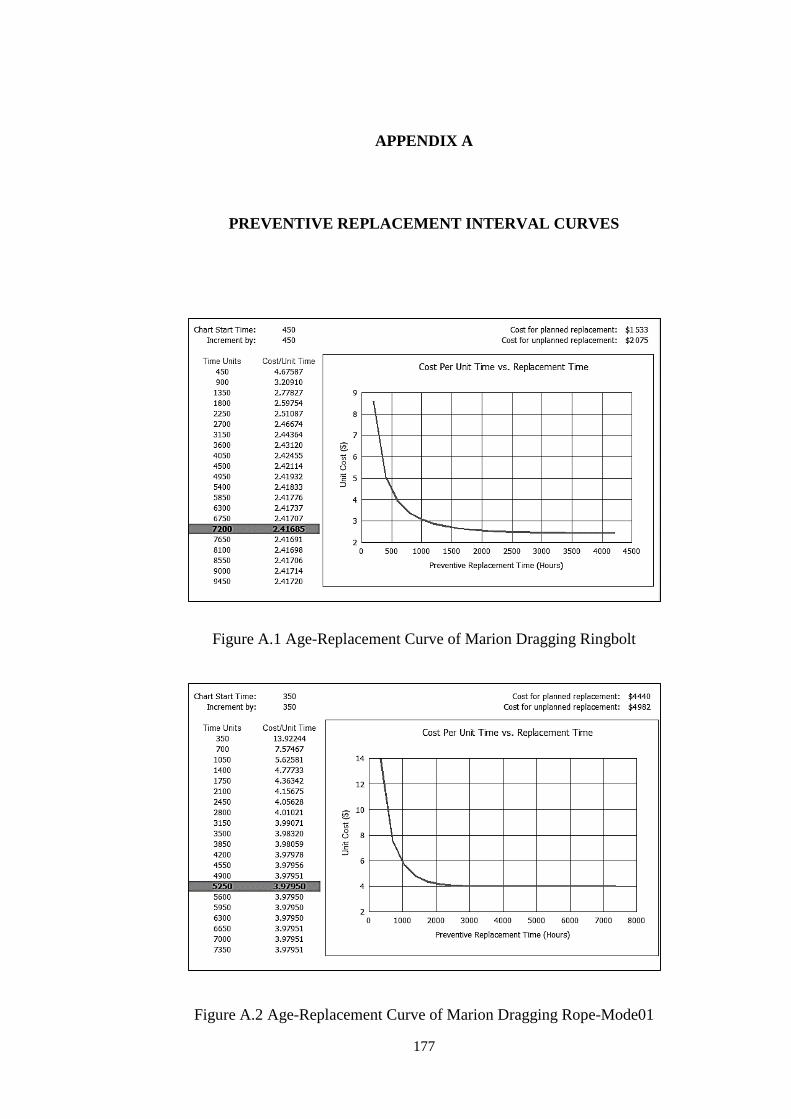
177

APPENDIX A

PREVENTIVE REPLACEMENT INTERVAL CURVES

Figure A.1 Age-Replacement Curve of Marion Dragging Ringbolt

Figure A.2 Age-Replacement Curve of Marion Dragging Rope-Mode01

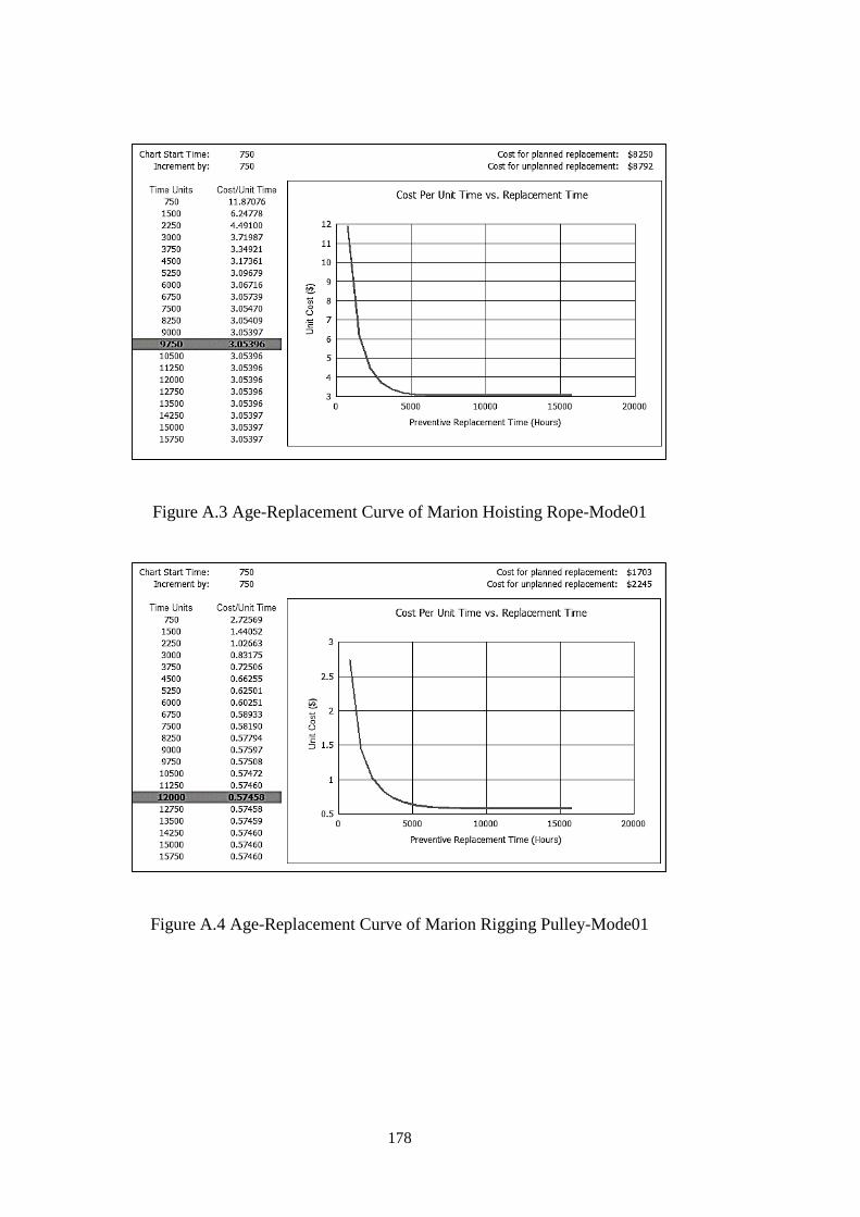
178

Figure A.3 Age-Replacement Curve of Marion Hoisting Rope-Mode01

Figure A.4 Age-Replacement Curve of Marion Rigging Pulley-Mode01

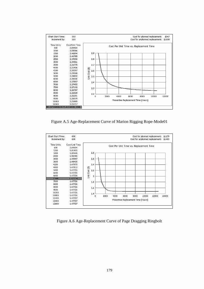
179

Figure A.5 Age-Replacement Curve of Marion Rigging Rope-Mode01

Figure A.6 Age-Replacement Curve of Page Dragging Ringbolt

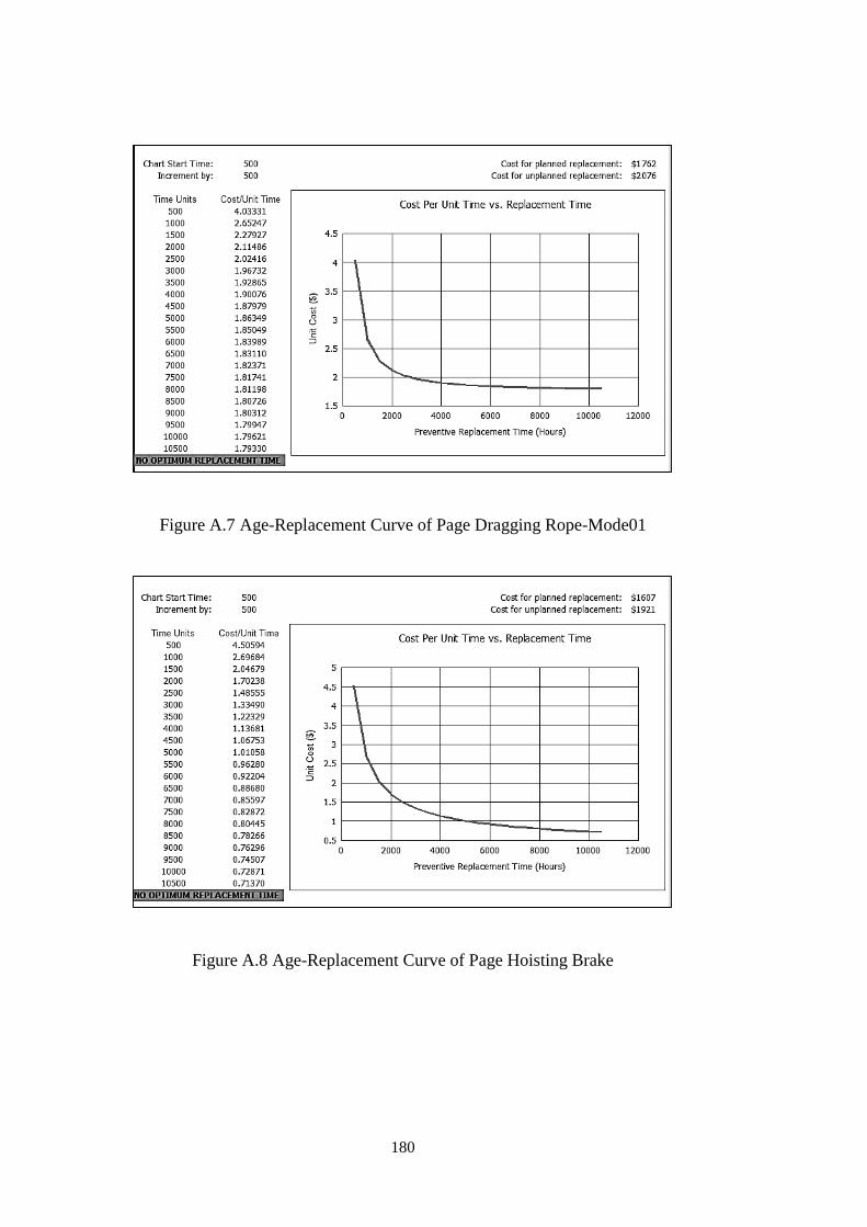
180

Figure A.7 Age-Replacement Curve of Page Dragging Rope-Mode01

Figure A.8 Age-Replacement Curve of Page Hoisting Brake

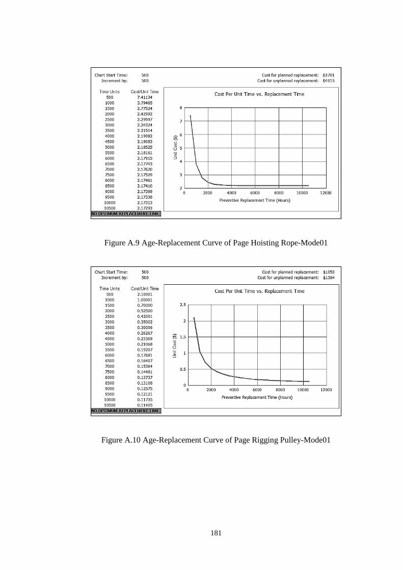
181

Figure A.9 Age-Replacement Curve of Page Hoisting Rope-Mode01

Figure A.10 Age-Replacement Curve of Page Rigging Pulley-Mode01

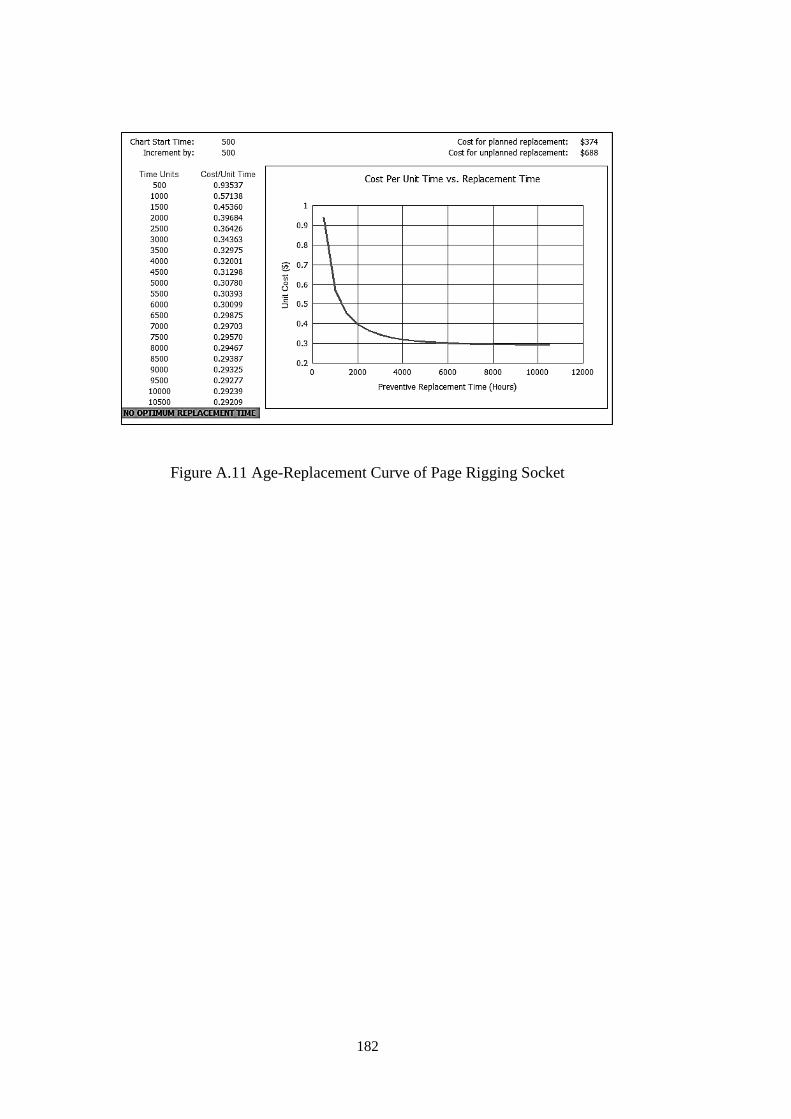
182

Figure A.11 Age-Replacement Curve of Page Rigging Socket

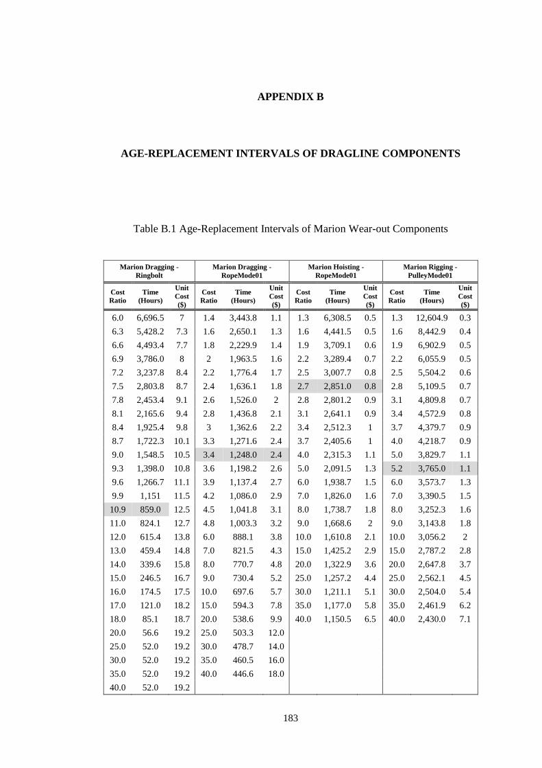
183

APPENDIX B

AGE-REPLACEMENT INTERVALS OF DRAGLINE COMPONENTS

Table B.1 Age-Replacement Intervals of Marion Wear-out Components

Marion Dragging -

Ringbolt

Marion Dragging -

RopeMode01

Marion Hoisting -

RopeMode01

Marion Rigging -

PulleyMode01

Cost

Ratio

Time

(Hours)

Unit

Cost

($)

Cost

Ratio

Time

(Hours)

Unit

Cost

($)

Cost

Ratio

Time

(Hours)

Unit

Cost

($)

Cost

Ratio

Time

(Hours)

Unit

Cost

($)

6.0 6,696.5 7 1.4 3,443.8 1.1 1.3 6,308.5 0.5 1.3 12,604.9 0.3

6.3 5,428.2 7.3 1.6 2,650.1 1.3 1.6 4,441.5 0.5 1.6 8,442.9 0.4

6.6 4,493.4 7.7 1.8 2,229.9 1.4 1.9 3,709.1 0.6 1.9 6,902.9 0.5

6.9 3,786.0 8 2 1,963.5 1.6 2.2 3,289.4 0.7 2.2 6,055.9 0.5

7.2 3,237.8 8.4 2.2 1,776.4 1.7 2.5 3,007.7 0.8 2.5 5,504.2 0.6

7.5 2,803.8 8.7 2.4 1,636.1 1.8 2.7 2,851.0 0.8 2.8 5,109.5 0.7

7.8 2,453.4 9.1 2.6 1,526.0 2 2.8 2,801.2 0.9 3.1 4,809.8 0.7

8.1 2,165.6 9.4 2.8 1,436.8 2.1 3.1 2,641.1 0.9 3.4 4,572.9 0.8

8.4 1,925.4 9.8 3 1,362.6 2.2 3.4 2,512.3 1 3.7 4,379.7 0.9

8.7 1,722.3 10.1 3.3 1,271.6 2.4 3.7 2,405.6 1 4.0 4,218.7 0.9

9.0 1,548.5 10.5 3.4 1,248.0 2.4 4.0 2,315.3 1.1 5.0 3,829.7 1.1

9.3 1,398.0 10.8 3.6 1,198.2 2.6 5.0 2,091.5 1.3 5.2 3,765.0 1.1

9.6 1,266.7 11.1 3.9 1,137.4 2.7 6.0 1,938.7 1.5 6.0 3,573.7 1.3

9.9 1,151 11.5 4.2 1,086.0 2.9 7.0 1,826.0 1.6 7.0 3,390.5 1.5

10.9 859.0 12.5 4.5 1,041.8 3.1 8.0 1,738.7 1.8 8.0 3,252.3 1.6

11.0 824.1 12.7 4.8 1,003.3 3.2 9.0 1,668.6 2 9.0 3,143.8 1.8

12.0 615.4 13.8 6.0 888.1 3.8 10.0 1,610.8 2.1 10.0 3,056.2 2

13.0 459.4 14.8 7.0 821.5 4.3 15.0 1,425.2 2.9 15.0 2,787.2 2.8

14.0 339.6 15.8 8.0 770.7 4.8 20.0 1,322.9 3.6 20.0 2,647.8 3.7

15.0 246.5 16.7 9.0 730.4 5.2 25.0 1,257.2 4.4 25.0 2,562.1 4.5

16.0 174.5 17.5 10.0 697.6 5.7 30.0 1,211.1 5.1 30.0 2,504.0 5.4

17.0 121.0 18.2 15.0 594.3 7.8 35.0 1,177.0 5.8 35.0 2,461.9 6.2

18.0 85.1 18.7 20.0 538.6 9.9 40.0 1,150.5 6.5 40.0 2,430.0 7.1

20.0 56.6 19.2 25.0 503.3 12.0

25.0 52.0 19.2 30.0 478.7 14.0

30.0 52.0 19.2 35.0 460.5 16.0

35.0 52.0 19.2 40.0 446.6 18.0

40.0 52.0 19.2

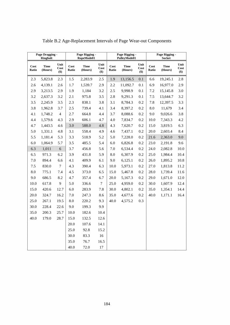
184

Table B.2 Age-Replacement Intervals of Page Wear-out Components

Page Dragging -

Ringbolt

Page Rigging -

RopeMode01

Page Rigging -

PulleyMode01

Page Rigging -

Socket

Cost

Ratio

Time

(Hours)

Unit

Cost

($)

Cost

Ratio

Time

(Hours)

Unit

Cost

($)

Cost

Ratio

Time

(Hours)

Unit

Cost

($)

Cost

Ratio

Time

(Hours)

Unit

Cost

($)

2.3 5,823.8 2.3 1.5 2,283.9 2.5 1.9 13,156.5 0.1 6.6 19,245.1 2.8

2.6 4,139.1 2.6 1.7 1,539.7 2.9 2.2 11,092.7 0.1 6.9 16,977.0 2.9

2.9 3,213.5 2.9 1.9 1,184 3.2 2.5 9,998.9 0.1 7.2 15,145.8 3.0

3.2 2,637.3 3.2 2.1 975.8 3.5 2.8 9,291.3 0.1 7.5 13,644.7 3.2

3.5 2,245.9 3.5 2.3 838.1 3.8 3.1 8,784.3 0.2 7.8 12,397.5 3.3

3.8 1,962.8 3.7 2.5 739.4 4.1 3.4 8,397.2 0.2 8.0 11,679 3.4

4.1 1,748.2 4 2.7 664.8 4.4 3.7 8,088.6 0.2 9.0 9,026.6 3.8

4.4 1,579.6 4.3 2.9 606.1 4.7 4.0 7,834.7 0.2 10.0 7,343.3 4.2

4.7 1,443.5 4.6 3.0 588.0 4.8 4.3 7,620.7 0.2 15.0 3,819.5 6.3

5.0 1,331.1 4.8 3.1 558.4 4.9 4.6 7,437.1 0.2 20.0 2,603.4 8.4

5.5 1,181.4 5.3 3.3 518.9 5.2 5.0 7,228.0 0.2 21.6 2,363.0 9.0

6.0 1,064.9 5.7 3.5 485.5 5.4 6.0 6,826.8 0.2 23.0 2,191.8 9.6

6.3 1,011 6 3.7 456.8 5.6 7.0 6,534.4 0.2 24.0 2,082.8 10.0

6.5 971.3 6.2 3.9 431.8 5.9 8.0 6,307.9 0.2 25.0 1,984.4 10.4

7.0 894.4 6.6 4.1 409.9 6.1 9.0 6,125.1 0.2 26.0 1,895.2 10.8

7.5 830.0 7 4.3 390.4 6.3 10.0 5,973.1 0.2 27.0 1,813.8 11.2

8.0 775.1 7.4 4.5 373.0 6.5 15.0 5,467.8 0.2 28.0 1,739.4 11.6

9.0 686.5 8.2 4.7 357.4 6.7 20.0 5,167.3 0.2 29.0 1,671.0 12.0

10.0 617.8 9 5.0 336.6 7 25.0 4,959.0 0.2 30.0 1,607.9 12.4

15.0 420.6 12.7 6.0 283.9 7.8 30.0 4,802.1 0.2 35.0 1,354.1 14.4

20.0 324.7 16.2 7.0 247.3 8.6 35.0 4,677.6 0.2 40.0 1,171.1 16.4

25.0 267.1 19.5 8.0 220.2 9.3 40.0 4,575.2 0.3

30.0 228.4 22.6 9.0 199.3 9.9

35.0 200.3 25.7 10.0 182.6 10.4

40.0 179.0 28.7 15.0 132.5 12.6

20.0 107.6 14.1

25.0 92.8 15.2

30.0 83.3 16

35.0 76.7 16.5

40.0 72.0 17

185

CIRRICULUM VITAE

PERSONEL INFORMATION

Surname, Name: Gölbaşı, Onur

Nationality: Turkish (TC)

Date and Place of Birth: 22 November 1984, İstanbul

Marital Status: Single

Phone: +90 506 634 05 73

Email: onurgolbasi@yandex.com

EDUCATION

Degree Institution Year of Graduation

MS METU Mining Engineering 2011

BS METU Mining Engineering 2007

High School Aliağa Super High School, İzmir 2002

WORK EXPERIENCE

Year Place Enrollment

2009-Present METU Mining Engineering Research Assistant

2009 MechSoft Software Solutions CAD Engineer

2008 GÜRSAN Construction Machines Co. Sales Engineer

FOREIGN LANGUAGES

Advanced English

186

PUBLICATIONS

1. Gölbaşı, O. and Demirel, N. (2015). Stress Investigation in an Earthmover Bucket

Using Finite Element Analysis: A Generic Model for Dragline. Journal of South

African Institute of Mining and Metallurgy, 115, 623-628.

2. Gölbaşı, O. and Demirel, N. (in press). Simulation of an Active Maintenance

Policy: A Preliminary Study in Dragline Maintenance Optimization. Current

Trends in Reliability, Availability, Maintainability and Safety.

3. Gölbaşı, O. and Demirel, N. (2015). Review of Trend Tests for Detection of Wear-

Out Period for Mining Machineries. The Proceedings Book of International Mining

Congress and Exhibition of Turkey (pp. 933-939). Antalya, Turkey: The Chamber

of Mining Engineers of Turkey.

4. Gölbaşı, O. and Demirel, N. (2014). Stochastic Models in Preventive

Maintenance Policies. Advanced Materials Research, 1016, 802-806.

5. Gölbaşı, O. and Demirel, N. (2013). Determination of Optimal Time Intervals

for the Dragline Maintenance Using Probabilistic Approaches. The Proceedings

Book of International Symposium on Mine Planning and Equipment Selection (pp.

1195-1203). Dresden, Germany: Springer International Publishing.

6. Demirel, N., Gölbaşı, O., Düzgün, Ş., and Kestel, S. (2013). System Reliability

Investigation of Draglines Using Fault Tree Analysis. The Proceedings Book of

International Symposium on Mine Planning and Equipment Selection (pp. 1151-

1158). Dresden, Germany: Springer International Publishing.

7. Gölbaşı, O. and Demirel, N. (2013). Reliability of Dragline’s Subsystems. The

Proceedings Book of International Mining Congress and Exhibition of Turkey (pp.

21-27). Antalya, Turkey: The Chamber of Mining Engineers of Turkey.

8. Gölbaşı, O., Demirel, N., and Tuncay, D. (2013). Failure Types of Draglines

and Their Classification. The Proceedings Book of Mining Machinery Symposium

and Exhibition of Turkey (pp. 47-55). İzmir, Turkey: The Chamber of Mining

Engineers of Turkey.

187

9. Gölbaşı, O., and Demirel, N. (2011). Stress and Deformation Distribution in a

Dragline Bucket Using Finite Element Analysis. The Proceedings Book of

Balkan Mining Congress (pp. 431-441). Ljubljana, Slovenia: Velenje Coal Mine.

10. Demirel, N. and Gölbaşı, O. (2011). Sonlu Elemanlar Analizi ile Çekme Kepçeli

Yerkazarın Kepçesi Üzerindeki Gerilmelerin İncelenmesi. Mining Turkey

Magazine, 50(3), 3-9.