Embed Size (px)
Citation preview
) ,CIVIL ENGINEERING SERIES STRUCTURAL RESEARCH 'SERIES NO. 322
RE-EXAMINATI N F THE THE RY SUSPENSI N BRIDGES
Metz Reference Room Civil Engineering Department BI06 C. E. Building University of Illinois Urbana,: Illinois 61801
by
H. H. WEST
and
A. R. ROBINSON
UNIVERSITY OF ILLINOIS
URBANA, ILLINOIS
JUNE 1967

A HE-EXAMINATION OF THE THEORY OF SUSPENSION BRIDGES
by
H. H. West
and
Ao Ro Robinson
L~IVERSITY OF ILLINOIS TJRBA.NA J ILLINO IS
JUNE 1967

ERRA.TA
Page Location Reads Should Read
2 Line 22 one on
6 Entry 7 in Notation (A~H)' .. for hangers (AflEH)i ... for ith
7
9
45
46
47
49
93
115
119
150
Entry 9 on page
Entry 1 on page
Line 1 after Eq. (3.34)
1
of some
Last of Eqs. (3.35) -v cose o 0
First o,f Eqs. (3.36) aS1sin2cpl
Equation number
In Eq. (3 . 37a )
Line 9
Second of Eq.
Vector (b1 ) of
Eq. (4.64)
Last line
Line 4
vT1=o' vT£=o
v v Tr=o' To=o
victor
b .. lJ
oM I / k (1 + ~ ! ) S
tenth
Line 1 after table *o~l£
Above title 56.0
hanger
I
at some
+v cose o 0
. 2e a S1sln 1
v =0, v =0 Tr To
vector
-k' oM/k (l+~') s s
twentieth
*o~ , 1£
54.8


ACKNOWLEDGMEN"T
This report was prepared as a doctoral dissertation by
Mr. F~rry H. West and was submitted to the Graduate College of the
University of Illinois in partial fulfillment of the requirements for
the degree of Doctor of Philosophy in Civil Engineering. The work was
done under the supervision of Dr. ,Arthur R. Robinson, Professor of
Civil Engineering.
The authors wish to thank Dr. JohnW. Melin, Assistant
Professor of Civil Engineering, for his invaluable assistance in planning
and developing the computer programs needed for this study.
During the course of the study, helpful comments on various
aspects of analysis and design of suspension bridges were contributed
by Dro Nathan Mo Newmark, Professor and Head of the Department of Civil
Engineering; Dr. James Eo Stallrneyer, Professor of Civil Engineering;
Mr. Jackson L. Durkee, Supervising Engineer of Bridges with the Bethlehem
Steel Corporation; Mr. George S. Vincent, formerly of the Bureau of
Public Roads; and Mes srs. Irvine P. Gould and Howard Silfin of r:Che
Port of New York Authority. Their respective contributions were of
great value.
The appropriation of funds by the University Research Board
for the use of the IBM, 7094-1401 system of the Department of Computer
Science is gratefully acknowledged.
TABLE OF CONTENTS
ACKNOWLEDGMENT~ . . . . LIST OF TABLES LIST OF FIGURES .
1.
2.
3.
INTRODUCTION.
1.1. 1.2. 1.3.
Object and Scope. . . .. Background Information .. Notation. . . . . . . . .
THE CLASSICAL DEFLECTION THEORY
2.1. Introduction... . . . . . . . . . . . . . . . . . . . 2.2. Description of the Mathematical Model of the Structure. 2.3. Development of the Theory ........... .
ANALYSIS USING A DISCRETE SYSTEM OF STRUCTURAL ELEMENTS
3.1. 3.2. 3.3. 3.4. 3.5. 3.6. 3.7. 3.8.
Description of the Mathematical Model Cable Equations . . . Compliance Conditions ... Stiffening Member . . . . . Suspension Bridge Equations Temperature Change. . . Hanger Elongations .. Newton~Raphson Method .
of the Structure.
Page
iii vi vii
1
1 3 5
15
15 15 18
24
24 27 43 47 49 56 59 62
4. ANALYSIS USING A CONTINUOUS STRUCTURAL SYSTEM . . . . . . .. 66
5.
4.1. Description of the Mathematical Model of the Structure
4.2. 4.3. 4.4. 4.5. 4.6. 4.7. 4.8. 4·9.
and Outline of the Analysis . . Cable Equations . . . . . . ~ . Equations of Stiffening Member. Suspension Bridge Equations . . . . . . . . . Linearized Equations. . .... Integration Procedure . . . . . . . Linear Solution . . . . . . . . . Newton-Raphs on Procedure.. .... Additional Comments About Continuous Formulation ..
NUMERICAL PROBLEMS: RESULTS AND EVALUATION ...
5·1. 5.2. 5· 3. 5.4.
Single-Span Unstiffened Suspension Bridge . . Hanger Elongations. . . . . . . . . . . . Shearing Deformation. . . . . . . . . . . Sample Problems for Three-Span Bridges.
iv
66 69 76 79 84 89 96
112 115
117
117 123 128 1.p:L
v
TABLE OF CONTENTS (Continued)
6. CONCLUSIONS AND RECOMMENDATIONS FOR FURTHER STUDY 0 •
6.1. General Conclusions .... 6.2 Recommendations for Further Study ..
LIST OF REFERENCES. Q
TABLES ..
FIGURES ...
APPENDIX A.
. ,
COMPUTER PROGRAMS.
A.l. A.2. A.3.
A.4.
STRESS .... Modified Version of STRESS . Program for the Discrete Analysis of Suspension Bridges . . . . . . . . . Program for the Continuous Analysis of Suspension Bridges . . . . . 0 • 0 •
APPENDIX B. LINEARIZED EQUATIONS FOR CONTINUOUS STUDY.
Page
138
138 141
144
147
159
190
190 190
191
191
193
Table
1
2
3
4
5
6
7
8
9
10
11
12
13
14
15
16
LIST OF TABLES
Algorithm for the Newton-RaphsonMethod (Schematically Shown in Figure 11). . .
Ini tial Values and Terminal Boundary Conditions for Case A (Single Span) .
Initial Values and Terminal Boundary Conditions for Case B (Single Span) .
Initial Values and Terminal Boundary Conditions for Case C (Single Span) .
Initial Values and Ter.minal Boundary Conditions for Case D (Single Span) .
Initial Values and Terminal Boundary Conditions for Case E (Single Span) .
Displacement Quantities Used in Imposing·Fictitiolls Boundary Conditions at Suppression Points . . ...
E~uation Numbers for Determining Loads PV and PH . . . .
Displacements for Problem 1.1 (See Sec. 5.1.1)~
Displacements for· Problem 1.2 (See Sec. 5.1.2) ...
Displacements and Moments for· Problem 2.1 (See Sec. 5.2.1). . . .. . ...
Displacements and Moments for Problem 2.2 (See Sec. 5.2.2) ...
Displacements, Shears and Moments (S ee Sec. 5. 3. 1) .
for·Problem 3.1
Displacements, . Shears and Moments for Problem 3.2 (See Sec. 5.3.2).. .
Displacements for Problem 4.1 (See Sec. 5.4.1).
Displacements and Moments for Problem 4.2 (See Sec. 5.4.2). . . .. . ...
vi
Page
148
148
15b
15.1
152
152
153
155
157
Figure
1
2
3
4
5
6
7
8
9
10
11
12
13
14
15
16
17
19
20
21
LIST OF FIGURES
Single-Span Suspension Bridge (Classical Deflection Theory)
Comparison of Response for Various Theories . . .
Chain System.
Typical Chain Element at Dead Load.
Live Load Displacements .
Restraints at Left Tower.
Anchorage Restraints ....
Stiffening Member Configuration
Configurations of Stiffened Suspension Bridges ..
Schematic Load-Displace.ment Diagram. . . . . .
Schmatic Diagram Illustrating the Newton-Raphson Method .
Cable Element . . .
Stiffening Member .
Support Condition for Single-Span Structure.
Support Condition at the Tower for Three-Span Structure 0
Schematic Representation of Newton-Raphson Procedure.
Description of Sample Problems ..
Displacement Diagrams for Problem 1.1 (See Sec. 5.101). . ...
Load-Displacement Diagrams for Problem 1.1 (See Seco 501.1)0 ....
Displacement Diagrams for Problem 1.2 (See Sec. 5.1.2).
Load-Displacement Diagram for Mid-Span of Problem 1.2 (See Sec. 5.1.2)0 . . .. . ........ .
vii
Page
159
160
163
164
165
166
167
168
170
170
171
172
173
175
Figure
22
23
24
25
27
28
29
30
31
32
33
viii
LIST OF FIGURES (Continued)
Displacement vSo 1/N2
for Problem 103 (See Sec. "50.l03)Q 0; 0 0 . 0 . 0 .
Displacement and Moment Diagrams for'Problem 2.1 (See Sec~ ;5~2~1)o ~ .............. .
Displacement and Moment Diagrams for Problem 2.2 (See Seco 5.202) ......... 0 ...... .
Changes Caused by Hanger Elongations (See Sec. 5.2.3) ..... 0 ••••••
Displacement, Shear and Moment Diagrams for Problem 3.1 (See Sec. 5.30l). 0 .. 0 0 0 . 0 0 .. . ..... .
Changes Caused by Shearing Deformations (See Sec. 5.303). . ..... .
Displacement Diagrams for Problem 4.1 (See Sec. 5.4.1) ........... .
Displacement and Moment Diagrams for Problem 4.2 (S e e Sec. 5 . 4. 2) . . . .. .... 0 • • • • •
Traversing Load Positions for Problem 4.3 (See Sec. 5.4.3)0 . 0 0 0 0 0 ••• 0
Horizontal Displacements for Various Load Positions for Problem 403 (See Sec. 5.4 .. 3). 0 • 0 ... 0 ••
Vertical Displacements for Various Load Positions for Problem 403 (See Seco 50403). . ....
Slopes for Various Load Positions for Problem 4.3 (S ee Sec. 5040.3) . 0 0 0 • 0 0 0 0 o. 0 . . . 0
Moments for Various Load Positions for Problem 4.3 (See Sec. 5.403). 0 • 0 0 • 0 0 0 . 0 .. 0 0 0 . 0
Page
177
178
179
180
182
184
186
188
1. INTRODUCTION
1.1. Object and Scope
The purpose of this investigation is to re-examine the
classical problem of static loading on suspension bridges. This problem
has been treated by many investigators for more than a century. The so
called IIdeflection theory" has emerged as the standard of suspension
bridge analysis. A brief summary of the development of the deflection
theory is presented in Chapter 2.
Most recent studies have dealt with computerized solutions of
previously developed methods of analysis or have presented a very general
formulation of the entire structural system. In the latter case, the
response of the cable and deck are not studied separately. However,
there has been no real effort since the advent of the digital computer
to re-examine the general formulation of the deflection theory and to
consider alternate methods of solution which are now computationally
feasible.
In this investigation, a general formulation of the deflection
theory is presented. Two independent methods of analysis are developed.
Each is based on a separate mathematical model; however, each model is
designed to reflect essentially the same set of basic assumptions
regarding the response of the structure. Special emphasis is given to
the techniques of solving the basic equations associated with each method
of analysis.
One method presented is a discrete method of analysis in which
the mathematical model can be composed entirely of discrete structural
1
2
elements. This a_pproach leads to a.matrixformulationof the governing
equations requiring ,the solution of_large numbers of nonlinear simul
taneousalgebraic equations .. This method is discussed.in Chapter-3.
The second method of analysis, presentedin_Chapter·4, is
based on a continuous formu~ationof the problem .. This continuous
treatment differs considerably from the classical deflection theory in
that horizontal cable displacements are admitted which eliminates any
_explicit "cable condition" of compatibility. In addition, nonlinear
terms are tre~ted fully. In this study,the problem is expressed as a
nonlinear boundary-value problem for o.rdinary.differe~tial equations.
The solution technique involves solving this boundary-value problem as
a set of initial-value problems. Serious 'numerical problems. are en
countered in.solving :the governing.differential equations and considera
ble attention is given to the'means of overcoming this difficulty.
,For each method of analysis, the Newton~Raphson procedure is
used as a device for solving the governing ,nonlinear equations. For the
continuous method of analysis, the Newton-Raphson procedure is applied
in a function space., This technique may, also be'applicable in solving
other nonlinear· systems whose behavior can be' expressed in terms of
systems of ordinary ,·differential equations 0
This investigation-is primarily concerned with the formulation
of the two separate methods of analysis. _Theemphssis is one the develop
ment of the theory. and on the methods of solution. ,No attempt is made to
perform an _ exhaustive parameter study. . A variety of problems is solved to
demonstrate the· application of each method of analysis and to compare the
_results .. The -solutions and discussions of these problems are presented in
Chapter 5.
3
Although this study deals only with a plane structure subjected
to static vertical loading, it can readily be seen that the methods
developed can be extended to investigate other aspects of suspension
bridge behavior. Such extensions are briefly discussed in Chapter 60
1.20 Background Information
The earliest presentations of the stiffened suspension bridge
theory all assumed that the distortions were small ~nough so that their
influence on the stress distribution could be ignored. This assumption
is a common one that is made in the analysis of all ordinary structures 0
Several theories based upon this assumption were proposed during the
nineteenth century. The most acceptable of these theories emerged as
the so-called "elastic theory," which is given in a very complete form
* by Stei~~an (1929) 0 It was used by some well into the twentieth
century a:'1d continued to be of use as an approximate method even after
more exac:, I:1ethods had been developed.
Early authors observed that suspension bridges suffered large
dis:,c~:i~~s ~hen live load was applied. J. Melan (1888) is generally
cre:::'i :'2:: ·,,'i:.h being the first to take account of this fact in the de-
velc~='2~: o~ :.he equations for a method of analysis that includes the
effec: :::::~ :.n'2 deflections on the stress distribution. This method of
analys:s !-las been called the "deflection theory.1I There has, however,
been so~e question about whether Melan should be credited with the
* An author's name followed by the publication date in parentheses denotes an entry in the List of References.
4
development of the deflection theory. Some authors credit W. Ritter
or Muller-Breslau with the development prior to Melan.
The deflection theory continued to develop through the efforts
of many engineers until it reached its classical form as presented by
Johnson, Bryan a~d Turneaure (1911). This treatment, as well as the
more general development by Steinman (1935), is founded upon an ex-:
ponential solution of the fundamental differential equation of the
deflection theory.
A series solution was presented by Timoshenko (1930,1943).
This solution was arrived at through the application of trigonometric
series to the solution of the differential equation. Many others have
used this approach in their studies.
The fundamental differential equation of the deflection theory
(Eq. 2.6) is nonlinear. Thus, the rules for superp'osition' that' corre~·
spond to linearity do not hold, and influence lines, as used in the
analysis of ordinary structures, cannot be applied in suspension bridge
analysis. This fact was recognized in the early days of the deflection
theory. However, it is possible to apply influence lines in a restricted
sense. Godard (1894) is credited with first statiilg:and'demonstta,ting.·
the correct application of influence lines to expedite the deflection
theory analysis of suspension bridges. Many other authors have dealt
with the subject of influence lines. Some of the more recent contribu
tors are Karol (1938), Peery (1956) and Asplund (1945, 1949, 1958, 1966).
With the advent of the digital computer, a new stimulus has
been provided for suspension bridge analysis. Here the problem has
frequently been discretized. The solution to a set of nonlinear
5
simultaneous algebraic equations then provides the desired displacementso
Most notable of these efforts are those of Asplund (1958, 1966). Also,
Poskitt (1966) and Saafin (1966) have recently contributed in this
area. These discrete computer studies invariably involve a relaxation
of some of the restrictive assumptions of the classical deflection theory,
but the theories vary in detail from author to author.
The above represents a brief outline of the historical develop
ment of the deflection theory. It is intended only to indicate some of
the most significant steps in its development.
In Chapter 2, the classical deflection theory will be treated,
and some of the above-mentioned contributions will be expanded upon. A
detailed historical account of the development of suspension bridge theory
is given by Pugsley (1957) and the development of the deflection theory
is presented in detail by Asplund (1945).
103. Notation
Each symbol is defined when it is first introduced in the texto
In this section, some of the most important symbols are explained for
the convenience of the reader 0
In Chapter 2, an effort is made to use symbols that are
frequently used in the literature on the classical deflection theory 0
Since this chapter is short, and all symbols are defined therein, these
symbols are not included in the summary below.
The discrete method and the continuous method are developed
in Chapters 3 and 4, respectively. Since the two methods involve
entirely different mathematical formulations, any common nomenclature
6
would be very difficult to maintain. Thus, the methods have their own
symbolic representations, which are summarized in Sections 1.3.1 and
1.302. Symbols which are used in only a limited portion of the text
and are not important in subsequent considerations are not included in
the following summary.
1.3.1. Notation for 'Discrete Method
aBl backstay stiffness at left anchorage
aSl saddle support stiffness at left anchorage
aBo backstay stiffness at right anchorage
aSo saddle support stiffness at right anchorage
A. cross-sectional area of ith element of chain system l
[AJ stiffness matrix for linear part of stiffened cable-support structure
[C J
[ Cij
J
(D)
E. l
cross~sectional area multiplied by modulus of elasticity for hangers
stiffness matrix for linear part of cable-support structure
submatrix 'of [C]
modified [C] matrix including the effects of temperature ::h2nge
,.
st;.br:a trix of [C '.' ] t
~c~al cable displacement vector referenced to known co:--.figuration
a:c~ulated cable displacement vector after ith linearization
= displacements resulting from the ith linearization about {D. I} with current (P.} as loads
l- l
modulus of elasticity of ith element of chain system
elongation of the ith element of the chain system at some known configuration
e id + e i £ = total elongation of the ith element of the
chain system
e i £
e it
[F]
[Fij
]
* [F ]
* .. [F' lJ]
hid
Hd
[ H]
K. l
£ . l
=
=
7
elongation of the ith element of the chain system due to live load and temperature change
free temperature elongation of the ith element of the chain system
[T]-l = inverse of cable stiffening matrix
submatrix,of [~J
flexibility matrix of stiffening member
* submatrix of [F ]
horizontal projection of the ith element of the chain system at some known configuration
horizontal component of force in each element of chain system at known configuration
expanded [RyJ matrix with zeros inserted in rows and columns corresponding to support points [H = T L + 1. See Eqs. (3.61)) (3.62) and (3.63)] r r r
A.E. l l
length of the ith hanger
length of the ith element of the chain system at some known configuration
dUT linear part of ---duo l
dUT linear part of ~ avo
l
dUT nonlinear part of ---duo l
dUT nonlinear part of ~ avo
l
vector of nonlinear terms with elements NHi
vector of nonlinear terms with elements NVi
(N i} V
(N}
(NHt }
(NVt }
(P}
* (P }
*~ (P .L}
(l~. } I l
* q. l-
* (Q }
(Q *i}
8
submatrix of (NV
}
total vector of nonlinear terms NHi and NVi
modified (NH} vector including effects of temperature change
modified (NV} vector including effects of temperature change
live load applied at point i to suspension bridge system
load vector with elements p. l
live load applied to stiffening member at point i
* load vector with elements Pi
* submatrix of (P }
equivalent horizontal load applied at ith node due to temperature change
equivalent load vector with elements p H. e l
equivalent vertical load applied at ith node due to temperature change
equivalent load vector with elements p V. e l
load vector--live load or modified live load
incremental load vector above known configuration
load vector for ith linearization--amount by which the applied loads differ from those satisfying Eq. (3.52) at (Di _l } (residual loads)
load vector that satisfiesEq~ (3.52) at displacement [Di
}
live load component concentrated at ith node of chain system
load vector applied to cable (hanger loads) with elements q. l
submatrix of (Q}
stiffening member reaction at point i
* reaction vector with elements qi
* submatrix of [Q }
R. l
SR· ~ l
t .. lJ
[TJ .:.t..
[T" ]
* .. [T lJJ
u. l
U T
v. l
V T
9
vertical projection of the ith element of the chain system of some known configuration
see Eq. (3018)
dUs non-constant terms from ~ ou.
l
dUs non-constant terms from --. dVi
vertical tower stiffness at left tower
horizontal tower stiffness at left tower
vertical tower stiffness at right tower
horizontal tower stiffness at right tower
temperature change
stiffness coefficient for stiffening member
cable stiffening matrix
stiffness matrix for stiffening member with elements t .. lJ
* submatrix of [T ]
horizontal displacement of ith node point
=~ final strain energy stored in the ith element of the chain system due to dead load, live load and temperature change
total strain energy stored in support restraints due to dead load, live load and temperature change
total strain energy in chain system due to dead load, li.ve load and temperature change
horizontal cable displacement vector with elements u. l
vertical displacement of ith node point
v. l
vertical deflection of stiffening member at point i
total potential energy due to dead load, live load and temperature change
10
vertical cable displacement vector with elements vi or vCi
submatrix of (VC}
deflection vector for stiffening member with elements vTi
w = intensity of distributed dead load
X. l
Y. l
Z. l
(El}
w
a .. lJ
A
AC
AdEd
(b}
(b £}
(b £}
horizontal coordinate of the ith node point of the chain system at some known configuration
see Eq. (3.14); X. =X' l + Xi2 , which are defined by Eq. (3.26) l l
= vertical coordinate of the ith node point of the chain system at some known configuration
=
see Eq. (3.26)
see Eq. (3.23)·
matrix with elements w 6t £. except for zeros inserted at l rigid support points
coefficient of thermal expansion
total potential energy of external loads due to dead load, live load and temperature change
potential energy of external loads due to dead load
Notation for Continuous Method
coefficients used in linear equations--see Appendix B
see Eqs. (.4.16)
crDss-sectional area of cable
cross-sectional area multiplied by modulus of elasticity for truss diagonal
vector of required boundary quantities with element~. bk
£th boundary quantity vector with elements b£k
vector of fictitious boundary conditions imposed at suppression point for £th solution with elements b£k
11
vector of displacement quantities at suppress10n point for the Ith unsuppressed solution with elements b£k
B = see Eqs. (4016)
c
d
D
E
see Eqso (4016)
constant to determine how much of the £.th unsuppressed solution must be included in forming the kth suppressed solution
general displacement quantity
see Eqs. (4.16)
see Eqs. (4.19)
modulus of elasticity for cable
flexural stiffness of stiffening member
cable sag at dead load
see Eqs. (4.19)
(g } the £th initial~value vector with elements gnk £ .t
G see Eqs. (4.16)
R(x) total horizontal component of cable force in deformed position
Rd(X)
R. l
oR. l
oR. 0 l ...
6[oHJ
horizontal component of cable force at dead load
* horizontal component of cable force at point i
variation in horizontal component of cable force at point i for final solution
variation in horizontal component of cable force at point i for £th solution
jump in the variation of horizontal component of cable force required at tower point--see Eqo (4.79)
* In the continuous study, the subscript i indicates the point where the quantity is being studied. For tower point, i=T; left of tower, i=L; right of tower, i=R; at terminal point i=t.
k s
~(x)
12
shear constant for Timoshenko beam
= hang.er.. :stiffne$s
K = see Eqs. (4.16)
~(x)
M(x)
Py(x)
PH(a)
p
r. l
r. l
R
tower stiffness
span length
hanger length
stiffening member moment
intensity of live load applied vertically to stiffening member
intensity of live load applied horizontally to cable
some incremented level of horizontal live load
= some incremented level of vertical live load
=
increment of vertical live load above some known level
vertical load level above PVo for accumulated displ~cements
horizontal load level above PHo for accumulated displacements
see Eq. (4.19)
intensity of horizontal component of dead load applied to cable
intensity of vertical component of dead load applied to cable
intensity of horizontal component of total load on cable in deformed position
intensity of vertical component of total load on cable in deformed position
intensity of hanger loads applied to stiffening member
see Eqs. (4.19)
terms used in linear equations--see Appendix B
= terms used in linear equations for Bernoulli-Euler beam with hanger elongations
see Eqs. (4.19)
s
s. l
s
t
13
final solution
ith solution--particular solution for i=O) homogeneous solutions for i ~ 0
kth suppressed solution
see E<1s. (4.19)
temperature change (above mean temperature)
see E<1s. (4.16)
see E<1s. (4.16)
V(x) stiffening member shear
w intensity of vertical dead load for conventional suspension bridge with vertical hangers
x
y =
ex
f3
r(x)
6
o(x)
0
TJ(x)
l1 i
OTJi£
s(x)
si
oSi£
horizontal coordinate at dead load and mean temperature
vertical coordinate at dead load and mean temperature
horizontal coordinate of cable in deformed position
vertical coordinate of cable in deformed position
vertical deflection of stiffening member
interval along structure between points where integration is performed
shear slope for Timoshenko beam
indicates a linear variation in the quantity that it prefixes (without parentheses) i.e. 011)
vertical displacement of cable due to live load and temperature change
l1(x) evaluated at point i
linear variation in 011' at point i for the £th solution
horizontal displacement of cable due to live load and temperature change
s(x) evaluated at point i
linear variation in Os at point i for the ith solution

5~i£
(n ) m
~m(i)
14
linear variation in 5~' at point i for the £th solution
the nth derivative of the mth unknown variable at point i
w = coefficient of thermal expansion

2. THE CLASSICAL DEFLECTION THEORY
2.1. Introduction
It is of interest to study the various linear theories that
have played a role in the evolution of the stiffened suspension bridge
theory. Each of these has served as a useful tool at some stage in the
history of suspension bridge analysis. It should be remembered that some
of the cruder early theories were quite adequate for the design of the
short, stiff suspension bridges common a century ago. However, as
spans increased, engineers were forced to devise more complicated
mathemat.ical models. Actually, some linear theories serve as a simple
introduction to some of the essential problems of the stiffened suspension
bridge. Nevertheless, all major modern bridges are such that linear
theories are unacceptable.
The deflection theory has been cast in many different formu
latio~s. This somewhat obscures the fact that all modern treatments of
the st~~~e~ed suspension bridge are basically deflection theory approaches
eve~ t,:-.:~g:-. t.he details may differ. In this chapter, the classical
foYC":..:~c:,::, ~:-. of the deflection theory will be briefly developed. This
~ill ;~s2e ~~ better perspective the formulations that follow in
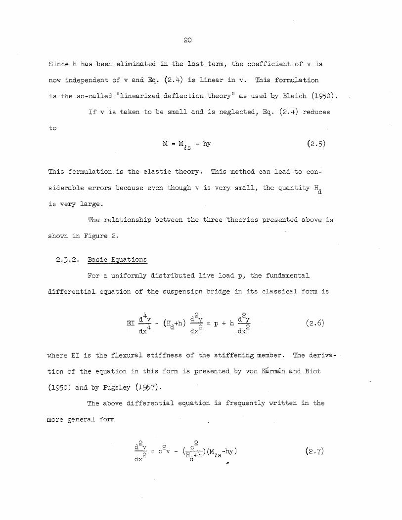
2.2, Description of the Mathematical Model of the Structure
The model of the stiffened suspension bridge that is considered
in formulating the classical deflection theory is shown in Fig~re 1. For
15
16
simplicity, only the main span is shown. The inclusion of the effect
of the side spans is not difficult.
The assumptions that are normally a part of the deflection
theory are as follows:
a) All stresses in the bridge remain within the limits of
proportionality and thus are determined by Hooke's Law. That is, there
is no physical nonlinearity.
b) The entire dead load of the structure is taken by the
cable. Thus, the stiffening member is unstressed at dead load and
mean temperature.
c) The cable is assumed to be perfectly flexible. This is a
good assumption as far as the stiffening member is concerned; local
flexural stresses in the cable can be investigated separately.
d) The dead load of the structure is taken to be uniform
along the horizontal projection. Thus, the initial curve of the cable
is parabolic. Jakkula (1936) demonstrates that about 80 to 85 percent
of the dead load is strictly along the horizontal. The remainder is
distributed along the cable or has the distribution determined by that
of the hangers.
e) For the determination of the additional cable tension
due to any live load distribution or to temperature change, the hanger
loads are assumed to be uniformly distributed. Several techniques are
available for deriving the "cable condition ll equation and these are
discussed in some detail by Jakkula (1936).
f) The hanger forces are taken as distributed loads as if the
distance between hangers were very small. The hangers thus form a
17
continuous sheet without shearing resistance. Of course, to get the
actual shears and moments in the stiffening member, the true nature of
the loading on the stiffening member must be considered.
g) In deriving the differential e~uation of the stiffening
member, the points of the cable are assumed to move along fixed
verticals. Several European authors have included the horizontal move
ment of the cable in their formulation of the e~uations of the deflec
tion theory, even though this refinement is generally abandoned before
the equations are solved.
h) The hangers are assumed to remain vertical during
deformation of the bridge.
i) The effects of the hanger elongations and tower shortening
under live load and temperature change is neglected. Johnson, Bryan and
Turneaure (1911) suggest that this effect is small for the case they
studied, while its inclusion greatly complicates the equations.
j) The horizontal component of cable tension is the same in
all spans. This requires that the towers are either on rockers or the
cable is mounted on saddles which are on rollerso Either of these
arrangements is considered obsolete; however, even in cases where the
saddles are fixed atop flexible, fixed-base towers, this assumption is
generally retained. For modern bridges this is still considered to be
an acceptable assumption because the towers are extremely flexible, and
the effect of the flexural stiffness of the tower does not introduce an
appreciable change in the horizontal component of cable tension between
main and side spans 0 This point is touched upon by Kuntz, Avery and
D~rkee (1958).
18
k) The stiffening member is ta.ken to be a beam of uniform
moment of inertia in each span. Thus, in the case of a truss, a beam
of equivalent moment of inertia is used. This ignores the shearing
deformation that can be considerable for truss-type stiffening members.
All of the above assumptions, with the exception of (b),
represent deviations from the true structure for the purpose of estab
lishing a tractable mathematical model of the structure. Assumption (b)
actually holds if the structure is properly erected and is, indeed, a
natural consequence of the erection procedures used.
A more detailed discussion of the effects of some of the above
assumptions is given by Asplund (1945).
2.3. Development of the Theory
In this section, a very brief discussion of the main features
of the classical deflection theory is presented. For greater detail,
the reade~ is referred to the list of references which are individually
noted th~ca&~out the text.
2.3.1. Je~era1 Nature of the Deflection .Theory
~ie basic equations of the deflection theory will be presented
for a si~g:e span bridge such as the one shown in Figure 1. Extension
to the tt~ee-span case merely involves similar equations for each side
span.
In accordance with assumptions (b) and (c) or Section 2.2, the
dead load moment on the stiffening member, Md , may be expressed as
o (2.1)
19
where Mds is the moment that the dead load would cause on the stiffening
member if it were a simply-supported beam, Hd is the horizontal component
of cable tension at dead load and y is the dead load ordinate of the
cable.
When live load is added or a temperature change occurs, the
same assumptions lead to a final moment on the stiffening member, M, of
(2.2)
in which Mis is the moment that the live load would cause on the stif
fening member if it were simply supported, h is the additional horizontal
component of cable tension produced by the application of live load and
temperature change and v is the vertical deflection of the cable and
stiffening member. Making use of Eq. (2.1), we can reduce Eq. (202) to
M = M - hy - (H +h)v is d
In all of the above expressions, the terms containing Hd or h
represent moments caused by the upward loads on the stiffening member
from the hangers.
Equation (2.3) includes the effect of the deflection v on the
moments of the stiffening member, whence, the name deflection theory.
Since h is dependent on v, Eq. (2.3) is nonlinear in v.
In most cases, since the dead load will greatly exceed the
live load, Hd will be much greater than h. For such cases, (Hd+h) ~ Rd ,
and Eq. (2.3) may be written in the form
M=M -~-Hv is d (2.4)
1
20
Since h has been eliminated in the last term, the coefficient of v is
now independent of v and E'l. (2.4) is linear in v. This formulation
is the so-called·"linearized deflection theory" as used by Bleich (1950).
If v is taken to be small and is neglected, E'l. (2.4) reduces
to
This formulation is the elastic theory. This method can lead to con-
siderable errors because even though v is very. small, the 'luantity Hd
is very large.
The relationship between the three theories presented above is
shown in Figure 2.
2.3.2. Basic Equations
For a uniformly distributed live load p, the fundamental
differential equation of the suspension bridge in its classical form is
where EI is the flexural stiffness of the stiffening member. The deriva-
tion of the equation in this form is presented by von ~rman and Biot
(1950) and by Pugsley (1957)·
The above differential equation is frequently written in the
more general form
2 c v -
21
2 Hd+h where c (~). This formulation was suggested by Steinman
(1929, 1935)·
Either of the above formulations involves two unknowns, the
function v and the single scalar h. Thus, an additional relationship
is needed. Using assumption (e) and either an energy or geometric
approach, we find this additional relationship to be
L
hi "w J AE :t:.. wti = Hd 0 vdx (2.8)
in which .2 is the length of the cable, AE is the axial cable stiffness,
w is the coefficient of thermal expansion, t is the temperature change,
w is the dead load intensity and L is the span length. This is not the
only form in which the "cable condition" e~uation is found. Jakkula
(1936) discusses this in some detail. For the three-span case, the
individual terms must be summed over the three spans.
2.3.3. Classical Solution
The solution of E~. (2.7) may be expressed as
v
where vh and vp are the homogeneous and particular solutions, respec
tively. Thus, we have
v (2010)
The particular solution vp depends upon the loading condition and Cl
22
and C2
are constants of integration to be determined by the boundary
conditions.
In the final form, v will be expressed in terms of known
quantities with the exception of h. For the evaluation of h, we must
substitute the final form of Eq. (2.10) intoEq. (2.8) and solve for h
by trial and error. The final equations are very complex and difficult
to handle. Once h is known, the expression for v is given by Eq. (2.10)
and expressions of moment, shear and load are readily determined.
Since the suspension bridge responds in a nonlinear fashion,
the above procedure must be carried out for each condition of loading
because superposition cannot be used. -A large number of cases have been
worked out by the above procedure and are tabulated by Johnson, Bryan
and Turneaure (1911) and by Steinman (1929).
2.3.4. Other Methods of Solution
There are several other methods that have been employed in
solving the basic equations of Section 2.3.2. A few will be mentioned
briefly here.
Timoshenko (1930,1943) presented a method for solving the
suspension bridge problem that employs trignometric series. In this
method, the right-hand side of Eq. (2.6) is expressed as a series and the
deflection v is also expressed as a series. The determination of the
coefficients of these series leads -to a final series expression for the
deflection v. The term h appears as part of the coefficients and must
be found before the complete expression for v is determined. This is
accomplished by a trial and error procedure that involves satisfying a
series expansion of Eq. (2.8). This method gained popularity because it
23
provided a more rapid process than did the classical method for cal-
culating the deflections and moments. Many other writers followed
Timoshenko's lead with series techni~ues and several computer programs
use a series approach. One of the most recent such treatments is that
by Kuntz, Avery and Durkee (1958).
Influence lines of a restrictive nature may be drawn for
suspension bridges. This is possible because E~. (2.6) can be thought
of as an e~uation for a beam with transverse load of magnitude
d2
(p + h ~) and a tensile force of magnitude (Hd+h). As is well known dx
[see for example Timoshenko and Gere (1961)] superposition can be employed
for such members as long as the axial force remains constant. A family
of influence lines can be prepared for all ~uantities of interest, each
for a different value of (Hd+h).
Karol (1938), Peery (1956) and Asplund (1945, 1949, 1958,
1966) are among the authors that have developed modified influence line
procedures.
3. ANALYSIp USING A DISCRETE SYSTEM OF STRUCTURAL ELEMENTS
3.1. Description of the Mathematical Model of the Structure
A model structure is developed for the analysis using a
discrete system of structural elements, representing the real structure
as closely as possible in every detail.
The most significant departure from the actual structure is
that the model structure includes a chain system as a replacement ,for
the cable. This chain system consists of a series of tension members
connected by frictionless hinges. This chain approximation for the
cable ignores th~ bending of the cable due to its own weight between
the hanger points. It also neglects the moment resisting capacity of
the cable at the hanger points, tower saddles and turn-down saddles.
These factors are believed to have little effect on the displacements
of the cable or the deflections, moments and shears of the stiffening
member. They do, however, cause considerable local effects on the cable,
as demonstrated by Wyatt (1960). The node points for the chain system
are free to displace in both the vertical and horizontal directions.
The stiffening member is represented in this analysis according
to the actual nature of the member. If the member is a truss, it is
treated as a truss, and the shear deformations which can be significant
in this type structure, are directly taken into account. If a solid-web
girder is used for stiffening, with either uniform or varying flexural
stiffness, it can also be handled directly with even greater ease.
Provisions are also made to handle the stiffening member directly
24
25
regardless of whether it is continuous or discontinuous at the towers.
For the stiffening member, only vertical deflections of the hanger
connection points are considered.
The supports for the stiffening member are assumed to be rigido
At the anchorage, the stiffening member is usually supported by the
anchorage itself and since this is taken to be rigid, this assumption is
correct. At the towers, the~e would be some small vertical movement of
the support. However, since the towers are massive and the truss
reaction quite small compared with the load input by the cable, these
movements are ignored.
Two possibilities are incorporated in the analysis to handle
the interconnection of the cable, saddle and tower at the tower tops.
In both cases, the mathematical model is designed on the assumption that
the cable is fixed in the saddle trough at a node point. The saddle may
be mounted on rollers such that it is free to move horizontally under
live load until the horizontal components of cable tension in the
adjacent spans are equal. The other possibility is that the saddle may
be fixed to the tower such that live load equilibrium is established by
bending of the tower. In either case, the saddle is supported vertically
by the tower 0 Thus, in addition to being restrained by adjacent links
of the chain system, the. saddle .node is. restrainedhor:izontally by the
flexural st.iffheSg-of··the tbwer'(unless·.the'.saddle is ;on rollers} ·and
vertically by the axial tower stiffness.
At the anchorages, the cables are also held by friction in the
troughs of the turn-down saddles 0 These saddles are assumed to be mounted
on rollers so that they are free to move in some specified direction in
26
the plane defined by the cable and stiffening member. The common move
ment of the end cable node point and the turn-down saddle depends on
the stiffnesses of the side-span cable, the backstay mechanism and the
saddle support frame. The stiffness of the side-span cable is determined
from the cable equations derived below, .whereas the stiffnesses of the
backstay mechanism and saddle support frame are assumed to be con
veniently represented by linearly elastic springs.
The large anchorage mass to which the backstays and saddle
supports are attached is assumed to be rigidly fixed. Likewise, the
foundations that support the towers are taken to be rigid.
In this analysis, provision is also made to consider hanger
elongations. The hangers are ~epresented by simple tension members;
their elongation can be directly included in the analysis if desired,
or the hangers can be assumed to be inextensible. It is possible to
handle cases with hangers between cable and roadway for all three spans
(loaded backspans) and those cases where there are only hangers in the
center span (unl9aded backspans).
In the real structure, the hangers become slightly inclined
when the structure deforms. This follows from the fact that each hanger
connection point at the cable is free to displace horizontally as well
as vertically, whereas the deck connection point is assumed to displace
vertically only. These inc Ilnati 0ns are very small, however, and it is
reasonable to neglect them.
The nonlinear response of the bridge is a result of the changes
of cable geometry. However, each structural element is assumed to behave
27
individually in a linear-elastic fashion. That is, there is no physical
nonlinearity, but geometric nonlinearity is considered.
As in the conventional deflection theory, it is assumed that
the total dead weight of the structure, including that of the cable, is
uniformly distributed horizontally. For the discrete analysis, this
loading is concentrated at the hanger points. It is also assumed that
the cable carries the entire dead load, and that the stiffening member
is unstressed under dead load at mean temperature. The dead load con
figuration of the structure is completely defined in this way.
3.2. Cable Equations
The chain system is shown in Figure 3 along with the coordinate
systerr. 2hosen. The hinges, or nodes, are located at potnts where the
cable is subjected to concentrated loads.
3.2.:. Dead Load Condition at Mean Temperature
I~ the case of dead load at mean temperature, the node points
fo~ ~~e :~~~~ system of each span are inscribed within a parabola. This
is ::':--. ::ee:;:::--.g with the assumption that the entire dead load of the struc
t'J~e :;S ;s-"::;::;::J:-ted by the cable and is uniform along the horizontal. Each
pa~at:_2. is d.efined by the end points and the prescribed sag for that
spa:' ..
A typical element of the chain at dead load and mean tempera
ture is shown in Figure 4. The length, vertical projection and horizontal
projection of the elementa~e denoted by Lid' rid and hid' respectively.
The subscript i indicates the ith element while the d denotes that these
28
~uantities correspond to the dead load configuration. The dead load
elongation, that is, the elongation of each element as a result of the
dead load acting alone, is denoted by e id . This ~uantity can be deter
mined from knowledge of the dead load horizontal component of the cable
tension, Hd (see Figure 4), and the resulting dead load configuration
of the system.
If Eid is the strain due to dead load in the ith element, then
Here, we make the assumption that the initial length of the element can
be replaced by the dead load length. The resulting expression is
in which A. and E. are the cross-sectional area and modulus of elasticity l l
of the ith element.
3.2.20 Dead Load Plus Live Load Condition at Mean Temperature
As live load is applied to the structure, each element in the
chain will be displaced in some general manner as indicated in Figure 5.
Here, horizontal and vertical displacements are specified by u and v,
respectively, the subscript indicating the node point.
The principle of minimum total potential [see Hoff (1956)] is
used to develop the e~uations for the determination of the live load
displacements. Thus, it is first necessary to determine an expression
for the strain energy stored in the cable at mean temperature under dead
load plus live load.
29
The additional elongation of the ith element due to live
loading, e i £, is
In order to express the strain energy, we need the final
elongation due to both dead load and live load. If we designate this
~uantity as eif , we obtain
=e·d+e· n l l(,t.
or
The final strain energy of the ith element is
Substituting in the above the expression for eif
from
E~, (304), we obtain
EiAi { 2 2 2 2 ----2L u. l+u.+v. l+v.-2u. lu.-2v. Iv.+2h· d (u. l-u.)+2r· d (v. I-v.) id l+ l l+ l l+ l l+ l l l+ l l l+ l
+2(e'd-L'd)(~(hod+U. l-u o)2+(r. ,,+Vo ·1-v.)2 - Llod ) + e2l'd
l l l l l+ l lao l+ l J
This expression for the final strain energy is in terms of
known ~uantities and the unknown live load displacements.
30
If there are n elements in the chain system, then the total
strain energy stored in the cable, UT, is
n
~ I i=l i=l
2 E.A.e·
f . l l l
2Lid
The potential energy of the external forces, i.e., external to
the cable, DT
, is
h n
h~i_l)d+hid hnd n+l
( ld) I I DT D - w VI - w ( 2 )v i - w (2)VD.+1 - q.v. d 2 l l
i=2 i=l (3.8)
where Dd is the potential energy of the external forces at dead load,
w is the dead load intensity and q. the additional hanger load at l
point i due to the live load.
The total potential energy, VT
, is the sum of the total cable
strai~ ehergy and the potential energy of the external forces and support
constrai~ts. Since the cable is assumed to be elastically restrained at
the su:;:p:;:::-: pcints, there is a strain energy, US' stored in the supports.
Thus,
or y-
on A 2 ---, .,tj •• e· f \ l l l
VT
+ U / 2Lid S '--!
i=l
- w
hld + Dd - w (2)~1
hnd (-2-)Vn+l -
i=l
n
I i=2
q.V. l l
he l)d+h'd W (l- l )
2 vi
(3.10)
31
3.2.3. Cable Displacement Equations
If we take the chain system to be composed of n elements, then
there are (n+l) nodes along the chain. It should be recalled here that
the cable support points are assumed to be elastically restrained and
that displacements of these points are admissible, although such dis-
placements are small compared with those along the span. Since there
are two displacements at each node point, we must have 2(n+l) equations
in order to determine the cable displacements. These equations are
determined from the minimum of the total potential, in which for cable
equilibrium, we have
(i=l, ... ,n+l)
Since u. and v. will enter in the strain energy expressions l l
only for the ith and the (i-l)th elements, Eq. (3.11) may be written as
(i=l, ... ,n+l)
We now concentrate on the determination of the first term in OU· f OU· f each of the above equations, i. e., ~ and ~ The corresponding au. av.
l l
terms for U(i-l)f are readily determined from these by changing certain
32
subscripts in a systematic manner while the partial derivatives of Us
and DT are quite easy to evaluate. dUif dUif In the derivation of the expressions for ~ and ~ , two
l l
different approaches can be used. In the first, the exact nonlinear
expressions are retained, whereas in the second, the equations are
truncated retaining only linear and quadratic terms. The exact method
will subsequently be devel.oped in .detail and the "truncatedfl method will
be briefly outlined.
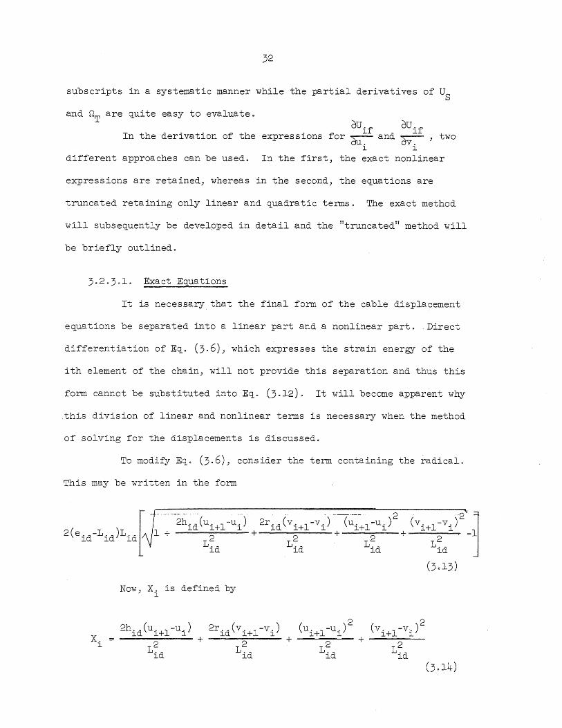
3.2.3.1. ExactEquations
It is necessary that the final form of the cable displacement
equations be separated into a linear part and a nonlinear part .. Direct
differentiation of Eq. (3.6), which expresses the strain energy of the
ith element of the chain, will not provide this separation and thus this
form cannot be substituted intoEq. (3.12). It will become apparent why
this division of linear and nonlinear terms is necessary when the method
of solving for the displacements is discussed.
To modify Eq. (3.6), consider the term containing the radical.
This may be written in the form
X. l
Now, X. is defined by l
2h . d ( u. l-u.) l l+ l
2 Lid
+ 2r· d (v. l-v.)
l l+ l
2 Lid
33
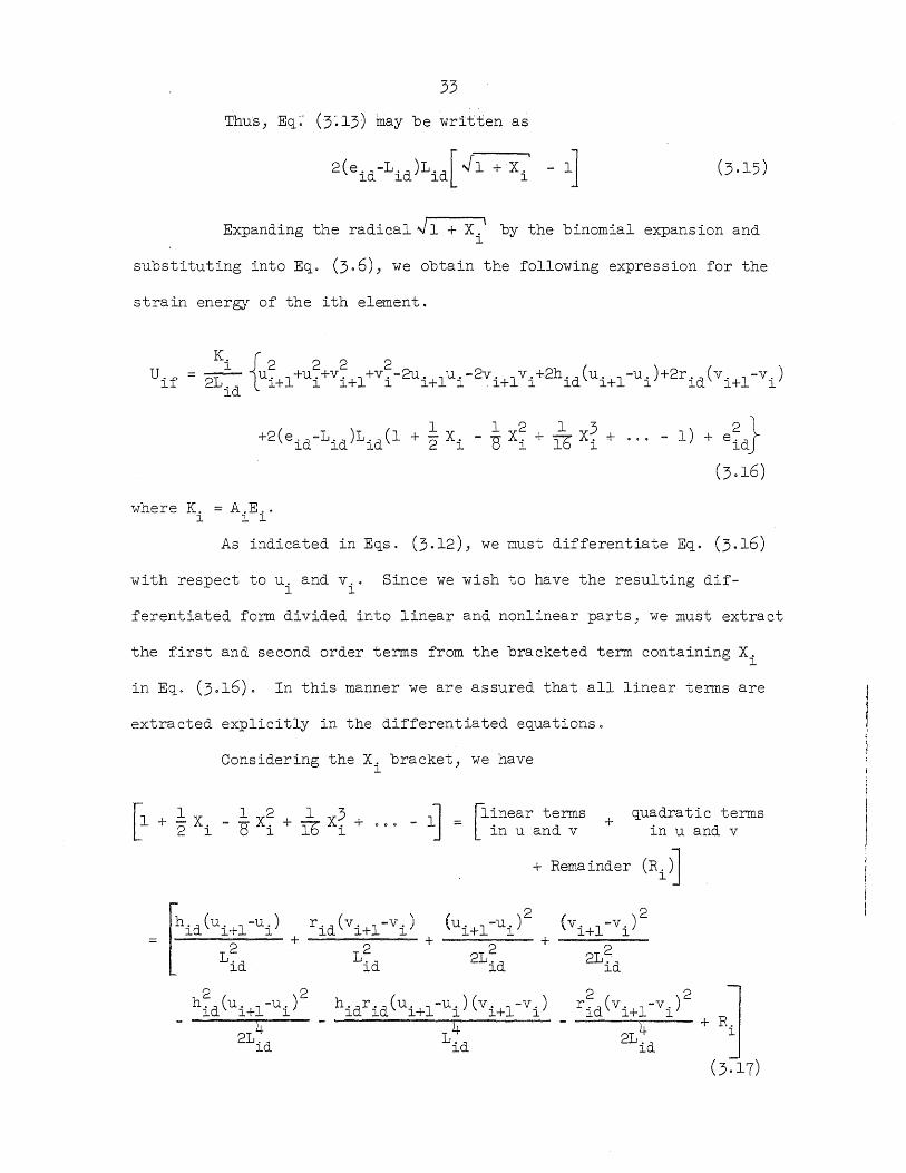
Thus)Eq~' (3'~13) may be written as
Expanding the radical.J 1 + X. I by the binomial expans ion and l
substituting into Eqo (3.6)) we obtain the following expression for the
strain energy of the ith element.
Ki {2 2 2 2 U
l' f = ----2L U. l+u.+v. l+v.-2u. lu.-2v. I v .+2h ·d(u. l-u.)+2r· d (v. I-v.) id l+ l l+ l l+ ll+ l l l+ l l l+ l
+2(eid-Lid)Lid(l + ~ Xi - ~ xi + ~ X~ + ... - l) + eia}
(3.16)
1-lhere K. = A.E .. l l l
As indicated in Eqs. (3.12)) we must differentiate Eq. (3.16)
with respect to u. and v.. Since we wish to have the resulting dif-l l
ferentiated form divided into linear and nonlinear parts) we must extract
the first and second order terms from the bracketed term containing X. l
in Eq. (3016). In this manner we are assured that all linear terms are
extracted explicitly in the differentiated equations.
Considering the X. bracket) we have l
rlinear terms + quadratic terms L in u and v in u and v
+ Remainder (Ri~
th'd(U. l-u.) r· d (v· 1 -v.) (u. l-u.)2
l l+ l l l+ l l+ l 2 . + 2 + 2 +
Lid Lid 2Lid
2 2 h·d(u. l-u.) l l+ l
4 2Lid
h·dr·d(u·+l-U.)(v. I-v.) l l l l l+ l
4 Lid
2 (v. I-v.)
l+ l
2 2Lid
2 2 r . d ( v. I-v.)
l l+ l
4 2Lid
where
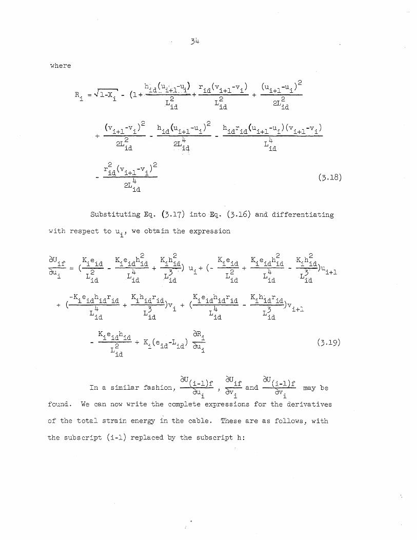
34
h'd(U"'l-U,) r'd(v, l-v.) R r.:--::::-'l X (1 l "" l+' -' l l l+ l
i = ".J .i-Xi - + ' 2 + 2 +
Lid Lid
2 (u, l-U') l+ l
2 (v, l-v,) l+ l
2 h'd(U' l-u,) l l+ l h·dr'd(u, l-u,)(v, l-v,) l l l+ l l+ l
+ ---2--2Lid
2 2 r. d( v. l-v,) l l+ l
4 2Lid
4 2Lict
4 Lid
Substituting Eq. (3.17) into Eq. (3.16) and differentiating
with respect to u i ' we obtain the expression
2 2 K,e'dh'd K,h'd
l l l ~) ( 4 + . ~ u, + -
3' l Lid Lid
-K.e'dh'dr'd (
l l l l + 4 +
Lid
K,h·dr'd K,e~dh'dr'd l l l) ( l l l l 3 vi + 4 -
Lid Lid
2 K,h'
d l l ) Y u i +l
Lid
K,h:.dr'd l l l) 3 ,v. 1
L l+ id
dU ( 1) dU l, f dU (l' -1) f In a . '1 f h' i- f d b Slml ar as lon, dUo ~ an dV, may e
l l l found. We can now write the complete expressions for the derivatives
of the total strain energy in the cable. These are as follows, with
the subscript (i-l) replaced by the subscript h:
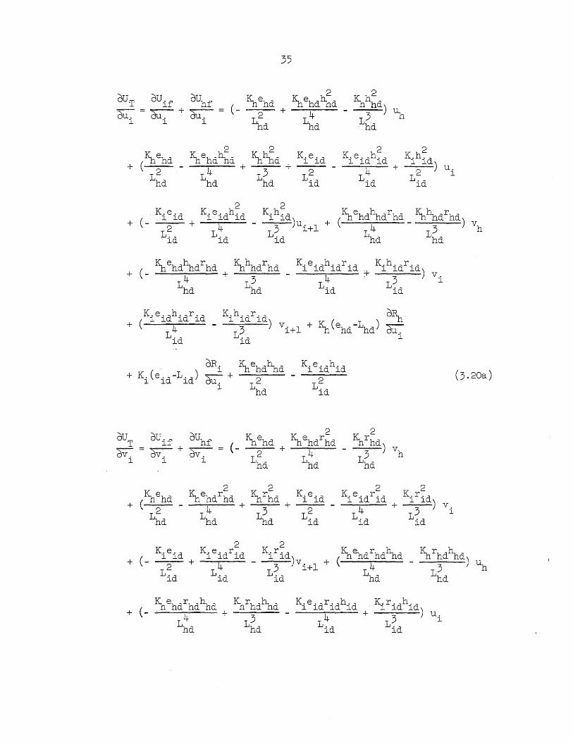
dUT dUif
dUhf (-
-Kbehd --~+~-dUo -. U,-
l l l
Kbehd 2
Kbehdhhd + ( 2 4 +
Lhd Lhd
2 K.e· d K,e'dh'd
+ (_ . l2l + l ~ l
Lid Lid
~d 2
~hhd 3
Lhd
35
2 2 Kbehdhhd ~hhd
+
~d 3 ) ~
Lhd
K,e' d 2 2
K,e'dh'd K,h'd l l l l l l l ) + 2 4 +
2 Lid Lid Lid
K.e'dh'dr'd K,h·dr· d l l l l + l l l) - 4 - 3 vi
Lid Lid
K.e·dh·dr· d K.h.dr' d dR (
l l l l _ l l l) ( )-h + 4 3 vi+l + ~ ehd-Lhd ~
Lid Lid l
dR. Kb ehdhhd + K. (e.d-L. d ) ~ l + --2-
l l l oul.
Lhd
dUhf Khehd 2 dU
T dU
if (-~ehdrhd
-~+--- + 4 ~ - v. dV.- 2 Lhd Lhd l l l
+ Kbehd
2 Kbehdrhd (-- 4 +
2 Lhd Lhd
2 K.e· d K.e·dr· d
( l l l l l
+ --2-+ 4 L. ~ L' d lQ l
2 K.e· d Kbrhd l l
3 +---
2 Lhd Lid
2
~rhd) v
h 3 Lhd
2 2 K.e·dr· d K.r· d l l l l l )
4 + 3
Lid Lid
u. l
v. l
K.e·dr·dh· d K.r.dh. d cR ( l l l l l l l) ( )-n
+ 4 - 3 u. 1 + Kb ehd -Ind ~ Lid Lid l+ l
CRi ~ehdrhd + K. (e·d-L· d ) ~ + --2--
l l l av. L l hd
In the above) Ri is as defined by Eq. (3.18) and ~ = Ri _l
is determined from Eq. (3.18) by replacing i and i+l by (i-l)=h and i,
respectively.
Equations (3.20) contain a linear part, a nonlinear part and
constant terms. Let us now concentrate on expanding the nonlinear
portion of these equationsQ For Eq. (3.20a), designating the nonlinear
portion by NHi
, we have
Consider the second term of Eq. (3.21). We can rewrite
Eq. (3.18) for R. in the form l
p _ .. ! l I v .L\. - 'i..J... T ./\..
l l
where
- (,1 + x.
l
2
z. = l
h·dr·d(u. l-u.)(v. I-v.) l l l+ l l+ l + 4
Lid +
2 2 r·d(v. I-v.) l l+ l
. 4 2Lid
Equation (3.22) is in a form that is undesirable for numerical
computations because it involves a relatively small difference of two
37
large quantities. This operation if carried out as indicated would
result in a loss of significant figures, and since the derivatives of
R. are multiplied by the large value of K.(e' d - L. d ) the results would l l l l
be unreliable. The same is, of course, true for the term involving ~o
This problem can be easily avoided by multiplying both
numerator and denominator of R. by {.Jl + X.' + (1 +!2 X. - z.)}· 0
l l l l
Upon performing this rationalization of the numerator, we get
R . l
1 2 .Z2. 2Z. - -4 X. + X.Z. ~ l l l l l
.Jl+Xil+ (l+~Xi-Zi)
Further simplificat~on of Eq. (3024) is possible by dividing
Xi into its linear and quadratic parts, Xil and Xi2, respectively, and
by introducing the new quantity Y.o Finally, we have l
where
R. ~ (4X Z .. - 2X X X2l' 2 - 4Z2
l.)
l 4Y. . i i il i2
Y. l
l
+ 2r . d ( v. I-v.)
l l+ l
2 Lid
2 2 (u. l-u.) (v. I-v.)
l+ l l+ l ------------ + ---------~ 2 2
Lid Lid
This expression for R. is free of the problem of loss of sigl
nificant figures that makes direct use of Eq. (3.22) difficult 0
Equations (3.22) through (3.26) can all be transformed to the
corresponding expressions for ~ by performing the subscript changes
that have been previously described.
Differentiating Eqo (3.25) and its companion expression for
Rh with respect to u i ' and substituting into Eq. (3.21), we get the
following equation for the nonlinear part of Eq. (3.20a):
Ki (eid ... L id ) r I ~r ~ ._.1 --- -- ---'- __ 2 ___ I ,.?', 4' X Z-l\T
+ 4Y~ L -LJ.AiLJiX i + CAilXi2Xi + Xi2Yi + 4ZiYi + i i.Li l
+ 4ZiX~i - 2XilXi2Yi - 2Xi2XIl Yi - 2Xi2X~2Yi - 8ZiZ~Ti} (3027)
In the above, primes denote differentiation with respect to u .. l
In like manner, the nonlinear part of Eq. (3.20b) can be
derived. We designate this quantity by NVi ; it is precisely the same as
NHi except that the primes are replaced by dots to indicate differentia-
tion with respect to v.~ l
Thus, the final expressions for the partials of the total
strain energy of the cable are Eqs. (3.20) with the nonlinear parts
replaced by NHi and NVi " If the linear parts of the right-hand sides of
Eqs. (3.20a) and (3020b) are called LHi and LVi' respectively, we have
K.e·dh· d l l l
2 Lid
we have
39
K.e·dr· d l l l
2 Lid
Returning now to Eq. (3.12) and using an abbreviated form,
dVT Khehdhhd K.e·dh· d dUS dDT + NHi +
l l l 0 (3·298. ) duo = LHi +--+---2 2 duo du.-
l Lhd Lid l l
i (1, ... , n+l)
dVT Khehdrhd K.e·dr· d dUS dDT + NVi +
l l l (3. 29b) -=L - + ~ + d-v."" - 0 dv. Vi 2 2 v. V.
l Lhd Lid·· l l
Recalling from Eq. (3.8) the expression for DT
, we can further
simplifY Eqs. (3.29). This formulation of DT assumes that all live
loads 2~e applied vertically. Thus, the partial derivatives of DT are
dJT
whld ~=--2--ql d '· "1
ev r~+l
whnd - --2 - ~+l
(i l, ... ,n+l) (3.30a)
(i 2, ... ,n)
Close examination of Eq. (3.298) reveals that the two constant
terms cancel. Physically, these quantities represent the dead load
horizontal components of force in the (i_l)th and ith elements and must
40
be equal at the dead load equilibrium configuration. InEq. (3~29b),
the constant terms are the vertical components of force in the (i_l)th
and ith elements respectively, and collectively they cancel the dead dDT
load contribution from ~ of Eqs. 13.30). At tower and anchorage avo
l
points, these constant terms are augmented by additional constant terms dUS dUS
that come from duo and "2iV: and represent the forces carried by the l l
supports at dead load. The sum of these constant terms must equal zero
in the case of Eq. (3.29a) and equal the dead load contribution from dDT . ~ In the case of Eq. (3.29b). This result expresses the fact that the avo
l
structure is in equilibrium at dead load.
The final cable equations are thus of the form
LHi + NHi + ~'Hi = 0 (3·31a)
(i = 1, ... ,n+l)
(3. 31b)
dUs dUS
where SRi and SVi are the terms remaining from ~ and dv. after the ·l l
constant terms have been cancelled.
For n segments, or (~+l)node points along the chain, the above
represents 2(n+l) simultaneous equations in the (n+l) unknown u and v
displacements of the node points. In matrix form, we may write the
above equations as
[C] ·fvj + ~, = {g}
In Eq. (3.32), [C] includes the linear terms LHi and LVi of Eqs. (3·31)
and also the terms from the support strain energy, SHi and SVi. The
41
support terms are linear because of the nature of the assumed support
restraints. This is discussed in detail in Section 3.3.3. The
~uantities (Uc} and (Ve} are the horizontal and vertical displacement
vectors respectively. Also, (NH
} and (NV
} are column vectors of nonlinear
terms which involve the properties of the linkage and the node displace
ments. The components of load applied to the cable are concentrated
at the node points along the cable and form the vector (Q}.
It is essential to note that the displacement vectors include
the support points. These support displacements are not taken to be zero
but are determined from the solution. Since the support restraints are
very stiff, these displacements are quite small. However) since a
method of analysis is desired that will permit a study of the effect
of these restraints, this treatment has been used.
3.2.3020 Truncated Equations
An alternate method of formulating the cable equations is to
return to Eq. (3.16) and drop all terms that are fourth order and
above in the node displacements. Thus cubic terms are the highest order
terms in the resulting expression for strain energy of the ith element
of the chain. After differentiation of the strain energy equation, we
have a linear part of a quadratic part.
We now proceed as before and again arrive at Eq. (3.32);
however) in this case (NH} and (NV
} are not the exact nonlinear forms,
but only the quadratic portions thereof.
This method was used in some early stages of the study. It
was found that for symmetrical loading the results from the truncated
equations agreed very closely with those from the exact equations. For
42
heavy non-symmetrical loading, agreement is not as good because the
response departs farther from a linear relationship.
In the studies made, the exact equations were used because
they presented no greater difficulty in programming than the trun
cated ones did once the equations were derived. The comparison of
computed results does demonstrate, however, that for symmetric loading
the nonlinear part is almost entirely a result of the quadratic terms.
3.2.3.3. Known Configuration
Throughout the development of the cable equations, reference
has been made to the dead load configuration. This configuration is a
known configuration and all the quantities which correspond to it have
been signified by the subscript d. Actually, what is required is some
known reference configuration to which the live load is applied. The
dead load configuration satisfies this requirement, but so does any
other k~ow~ configuration to which an additional amount of live load is
to be app2.ied. Also, it has been implied in the development that the
live loa j -,'e :::::,or represents the entire live load distribution. Actually,
these eq~&:i~~s are valid for finding the displacements relative to any
known co~:i~~ration (denoted by the subscript d) that are caused by a
live loa j ";e ::cr that represents the applied portion of the live load.
T~is is an essential point for the full understanding of the
numerica: procedure used to solve the equations. This procedure
generally requires that the live load be applied in several increments.
The first increment uses the dead load configuration as the known con
figuration and the solution leads to a new equilibrium configuration.
For the next increment, the known configuration is the resulting
43
equilibrium configuration from the previous increment. This process
continues until the entire live load is on the structure.
The numerical procedure, which is in essence the Newton-
Raphson method, will be discussed in detail in Section 308.
3.30 Compliance Conditions
3.3.1. Tower Compliance
The node points of the chain system located at the tower
saddles have restraints against movement in addition to those provided
by the adjacent linkage elements. These restraints are assumed to be
represented by linear springs with vertical and horizontal stiffnesses
of magnitude tv£ and t H£, respectively, for the left tower and tVr and
tHr for the corresponding quantities for the right tower. This
arrangement is shown schematically in Figure 6 for the left tower. The
vertical and horizontal springs represent the axial and flexural stiff-
nesses of the tower in those cases where the saddle is attached to the
tower. If the saddle is free to move on rollers the horizontal spring
has zero stiffness while the vertical spring still corresponds to the
axial stiffness of the tower.
The strain energy stored in the towers at dead load plus live
load is
44
where the subscripts £ and r refer to left and right tower, respectively,
and d signifies dead load.
It should be noted that tHt and t Hr are not actually linear
because as the live loading is applied, the tower loads increase and
* the flexural stiffness of the tower decreases. However, in the
numerical procedure used to solve for the displacements the live load is
applied in increments, and within each increment several linearizations
are made until the correct displacements are found (see Sec. 3.8).
Accordingly, the stiffnesses t H£ and tHr are recomputed for each
linearization using the tower loads that are acting at the latest level
of live loading. Thus, the nonlinear response of the tower is traced
even though linearity is assumed at any given level.
The flexural stiffness of the tower is computed by the
numerical method developed by Newmark (1943). The computer program
provides for subdividing the tower into ten main sections. These
sections need not be of equal length. .Each main section can be further
divided into ten equal sections. .At any level of live loading, vertical
loads imposed on the tower by the cable and truss reactions are taken
as the tower loads. A linearly elastic rotational spring is provided
at the base so that the effect of base rotation can be studied. The
moment variation along the tower is taken to be polygonal and thus the
trapezoidal rule is used to compute the concentrated angle changes.
3.302. Anchorage Compliance
The turn-down saddles provide the end node points for the chain.
In addition to the restraint provided by the adjacent links, these node
* The results of computation show that this refinement is of little conseq~enceo
45
points are restrained against movement by the stiffnesses of the back-
stay arrangement and the saddle support frame. These stiffnesses are
designated as aBl and aSl ' respectively, for the left anchorage and,
with (n+l)=o, aBo and aSo for the right anchorage. The complete
anchorage arrapgement is shown in Figure 7· In terms of ~l' ~o' 81 and
8 , as indicated in Figure 7, and with a and ~ as the assumed coordinate o
axes, the strain energy in the anchorage mechanism is
In the above, sid and bid are the dead load extensions of the support
and backstay restraints at the left anchorage, Sod and bod have similar
meaning for the right anchorage, /1 = ~l - 81 and / = ~ - 8 o 0 0
In addition, we have the relations
<Xl ul cos 81 - vl sin 8
1
~l ul sin 8
1 + vl cos 8
1
a ·-u cos 8 v sin 8 0 0 0 0 0
t30 -u sin 8 - v cos 8
(3.35) 0 0 0 0
We assume that as the turn-down saddle displaces, the direction
of the backstay remains unchanged. This seems reasonable since the dis-
placements are small relative to the length of the backstayo
46
303.3. Support·Strain.Energy
The total strain energy stored in the supports,US
' is the sum
of the strain energies in the tower and anchorage restraints. Thus, we
must add Eqs. (3.33) and (3.34) to obtain US' which was first intro
duced in Eq. (3.9). Differentiation of Us yields the following:
dUS HId dU
I =
dU S Vld dVI
=
dU ~ = H + (aB cos2~ +as sin2e )u + (aB sin~ cos~ -aSlsine cose )v dU od 0 0 0 0 0 0 0 D 0 0 0
o
dUS 2 ~v = Vod + (a_ sin~ cos~ -aSlsine cose )u + (aB sin ~ +as cos
2e )v
o EO 0 0 0 0 0 0 0 0 0 0 o
In the above, Hid and Vid are constant terms which represent
the total horizontal and vertical components of force, respectively,
tak:en at dead load by the support at point i. These constant terms are
those that were discussed in the paragraph following Eqs. (3.30); they are
needed to satisfy dead load equilibrium. Of course, as previously
47
stated, these constant terms cancel (in pairs) and are not present in
Eq. (3.32).
The remaining terms from Eqs. '(3.36) are those that were
previously called SHi and SVi and augment the cable terms LHi and LVi
to form the matrix [C] of Eq. (3.32). It should be noted that the
support terms enter only into the coefficients of the support displace-
ments for the equations that involve equilibrium of these support pointso
3.4. Stiffening Member
The stiffening member of a suspension bridge can be thought of
as a beam on rigid supports at the anchorages and towers, and supported
non-rigidly at the hanger support points. This beam is continuous over
the hanger support points but may be either continuous or discontinuous
through the towers. These two possibilities are shown in Figure 8. In
matrix form,
relation
tll
til
trl
the response of the stiffening member is governed by the
t l £
t££
t r £
t lr
t£r
t rr
t or
tlo
t£o
t ro
t 00
v Tl=o
vT2
vT £-1 , v
Tl=o vT,£+l
v· T r-l
v ' Tr=o v T,r+l
vTn v
To=o
p* 1
p* 2
p* £
p* r
p* o
q* 1 q* 2
* q£
~
48
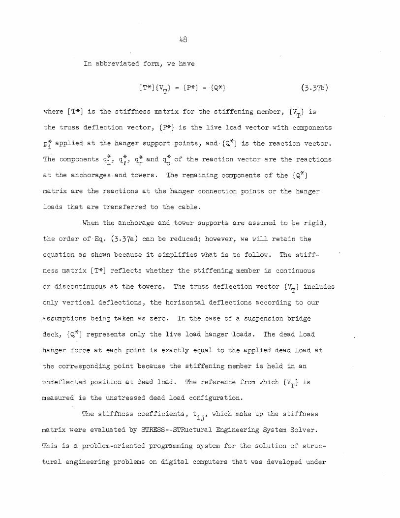
In abbreviated form, we have
[T*](VT} = (P*} - (Q*}
where [T*] is the stiffness matrix for the stiffening member, (VT
} is
the truss deflection vector, (P*} is the live load vector with components
p~ applied at the hanger support points, and (Q*} is the reaction vector. l
, * * * The components ql' q£, ~ and qo of the reaction vector are the reactions
at the anchorages and towers. The remaining components of the (Q*}
matrix are the reactions at the hanger connection points or the hanger
loads that are transferred to the cable .
. When the anchorage and tower supports are assumed to be rigid,
the order of Eq. (3.37a) can be reduced; however, we will retain the
equation as shown because it simplifies what is to follow. The stiff-
ness matrix [T*] reflects whether the stiffening member is continuous
or discontinuous at the towers. The truss deflection vector (VT
} includes
only vertical deflections, the horizontal deflections according to our
assumptions being taken as zero. In the case of a suspension bridge
deck, (Q*} represents only the live load hanger loads. The dead load
hanger force at each point is exactly equal to the applied dead load at
the corresponding point because the stiffening member is held in an
undeflected position at dead load. The reference from which (VT
} is
measured is the unstressed dead load configuration.
The stiffness coefficients, t .. , which make up the stiffness lJ
matrix were evaluated by STRESS--STRuctural Engineering System Solver.
This is a problem-oriented programming system for the solution of struc-
tural engineering problems on digital computers that was developed under
49
the direction of Fenves (1965a,1965b). The stiffness coefficients need
not be evaluated by STRESS; indeed, an independent scheme could easily
be programmed. STRESS was used for this study because it was available
and convenient. The details concerning the makeup of STRESS and its
use in this study are discussed in Appendix A.
3.5. Suspension Bridge Equations
The determination of the displacements of a loaded cable is a
subject that can be handled readily by Eq. (3.32) as long as the initial
shape of the cable is known and the load victor is defined. This equa-
tion is directly applicable in the case of the unstiffened suspension
bridge where the initial shape of the cable is assumed to be parabolic
under dead load and the load vector (Q) comprises the full live load.
Here, the bending stiffness of the deck is considered negligible and
thus it does not act to distribute the live load to the cable.
For the stiffened suspension bridge, the cable does not carry
the full live load since the stiffening member absorbs some load as it
deflects. More important, however, is the fact that the stiffening
member acts to distribute the load in a more uniform manner to the
cable.
The primary concern in this study is the stiffened suspension
bridge, and the development of some of the relations governing its
behavior is the subject of this section. Many different arrangements
are commonly used for stiffening a suspension bridge, and several of
these systems will be discussed here. At this time, we shall not con-
sider the effect of hanger elongations or temperature change. These
50
topics will be discussed in later sections. Throughout the current
discussion, we shall consider the case of a three-span structure.
3.5.1. Cable Stiffening Matrix
Figure 9 shows some of the more common arrangements for the
three-span stiffened suspension bridge. Let us consider first the case
of the bridge with loaded backspans; that is, hangers are provided
between the cable and deck in all three spans of the bridge.
Considering the cable alone, we see that (Q} of Eq. (3.32)
must have zero elements at the anchorage and tower points since there are
no hangers at these points. For the remaining points, we note that each
element of (Q} is equal to the corresponding element of (Q*} in
Eq. (3.370). Physically, these elements represent the hanger load at
each point. Thus, we have
q. l
q. l
o
qf l
(i=l,£,r,o)
( i =2, q 0 • , £ -1; £ + 1, . 0 • , r -1 ; r+ 1 -' . . . -' n )
Also, since we are presently assuming the hangers to be in-
extensible, we know that the vertical displacements of the cable are
equal to the vertic~l truss deflections at all points except the anchorage
and tower points. Thus,
(i=2, ... ,£-1; £+l, ... ,r-l; r+l, .. ,n)
In or~er to develop a convenient matrix formulation for the stiffened
structure, it would be best to express the stiffening effect that the
truss has on the cable in terms of the full vertical cable displacement
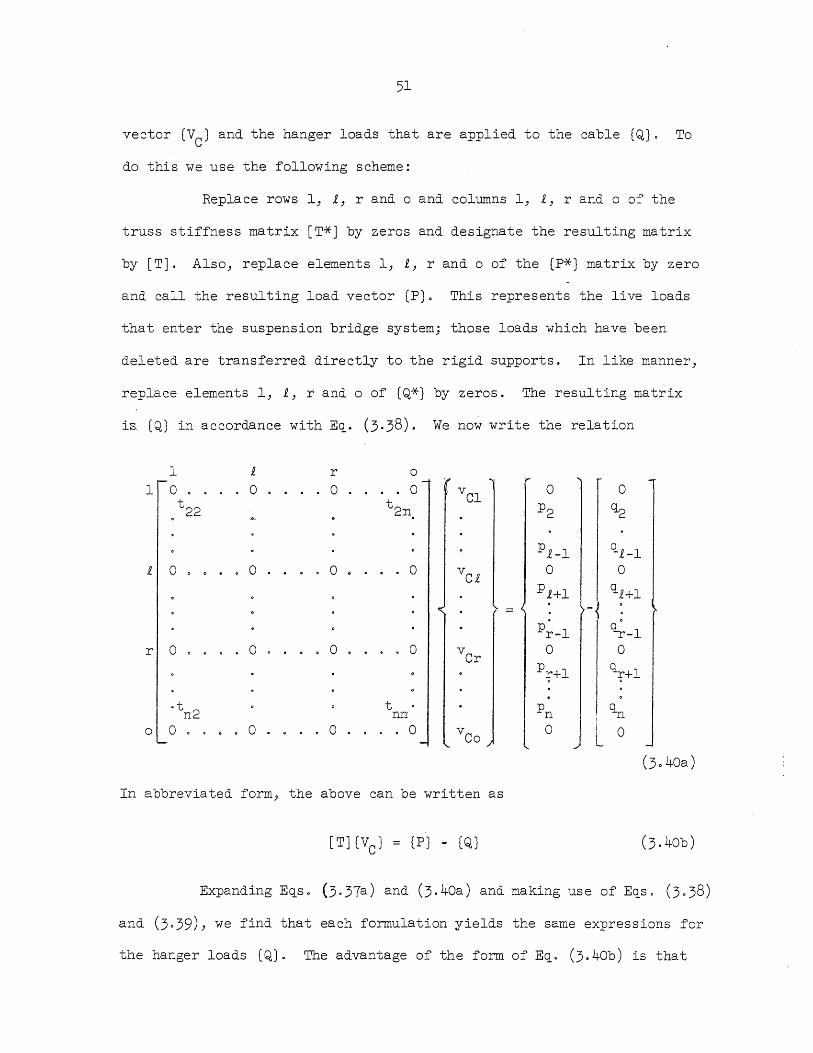
51
vector (VC
) and the hanger loads that are applied to the cable (Q). To
do this we use the following scheme:
Replace rows 1, £, rand 0 and columns 1, £, rand 0 of the
truss stiffness matrix [T*] by zeros and designate the resulting matrix
by [T]. Also, replace elements 1, £, rand 0 of the (P*) matrix by zero
and call the resulting load vector (P). This represents the live loads
that enter the suspension bridge system; those loads which have been
deleted are transferred directly to the rigid supports. In like manner,
replace elements 1, £, rand 0 of (Q*) by zeros. The resulting matrix
is (Q) in accordance with Eq. (3.38). We now write the relation
£ r o .... 0
£ 0 .... 0 .... 0 .... 0
r 0 0 0 . 0 vCr
·t n2 t
nn 0 0 0 0 0 vCo
In abbreviated form, the above can be written as
[T](VC
} = (P) - (Q)
o ~
P£-l q£-l 0 0
P£+l q£+l -{
~-l Pr-l 0 0
Pr+l qr+l
Pn
J qn
0 i 0 L (3. 40a)
Expanding Eqs. (3.37a) and (3.40a) and making use of Eqs. (3.38)
and (3.39), we find that each formulation yields the same expressions for
the hanger loads (Q). The advantage of the form of Eq. (3.40b) is that
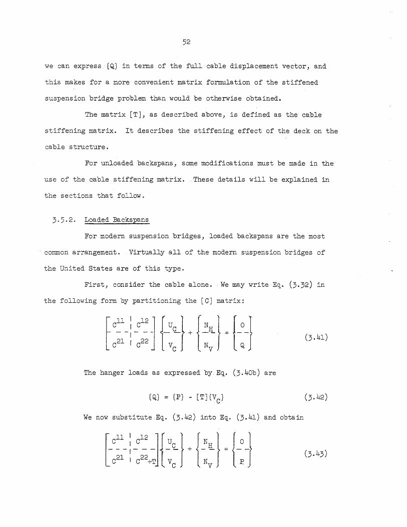
52
we can express (Q} in terms of the full cable displacement vector, and
this makes for a more convenient matrix formulation of the stiffened
suspension bridge problem than would be otherwise obtained.
The matrix [T], as described above, is defined as the cable
stiffening matrix. It describes the stiffening effect of the deck on the
cable structure.
For unloaded backspans, some modifications must be made in the
use of the cable stiffening matrix. These details will be explained.in
the sections that follow.
3.5.2. Loaded Backspans
For modern suspension bridges, loaded backspans are the most
common arrangement. Virtually all of the modern suspension bridges of
the United States are of this type.
First, consider the cable alone .. We may writeEqo (3.32) in
the following form by partitioning the [C] matrix:
The hanger loads as expressed by.Eq. (3.4ob) are
(Q} = (P} - [T](VC}
We now substitute Eq. (3.42) into Eq. (3.41) and obtain
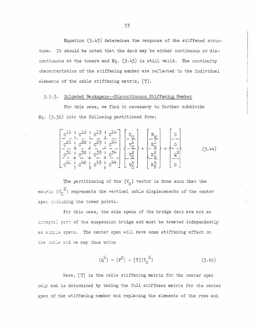
53
Equation (3G43) determines the response of the stiffened struc-
ture. It should be noted that the deck may be either continuous or dis-
continuous at the towers and Eqo (3.43) is still valid. The continuity
characteristics of the stiffening member are reflected in the individual
elements of the cable stiffening matrix) [TJ.
305.3. Unloaded Backspans--Discontinuous Stiffening Member
For this case) we find it necessary to further subdivide
Eq. (3.32) into the following partitioned form~
ell 1 e12 I e13 I e14 _UQ.. l!~ -:-[ - - 1 _ _ L _ .L ~
e 21 I e22 I e23 I e24
~ Nl ---l- -..J - -1--
+ rN~ = (3.44) e31 I e32 I e33 I e34 .~ -:~[ ---t-+-+-- -L e 41
1 e 42 I e43 I e 44 v3 N3 , , I e v
The partitioning of the eVe) vector is done such that the
(V~2) represents the vertical cable displacements of the center v
spa~ ~~:l~ii~g the tower points.
Fer this case) the side spans of the bridge deck are not an
~:-.-:e~r:;;._ ]:2.r: of the suspension bridge and must be treated independently
as s~~;:e spa~s. The center span will have some stiffening effect on
the ::;;'-:::02 3.:-.::1 'we may thus write
Here) [TJ is the cable stiffening matrix for the center span
only and is determined by taking the full stiffness matrix for the center
span of the stiffening member and replacing the elements of the rows and
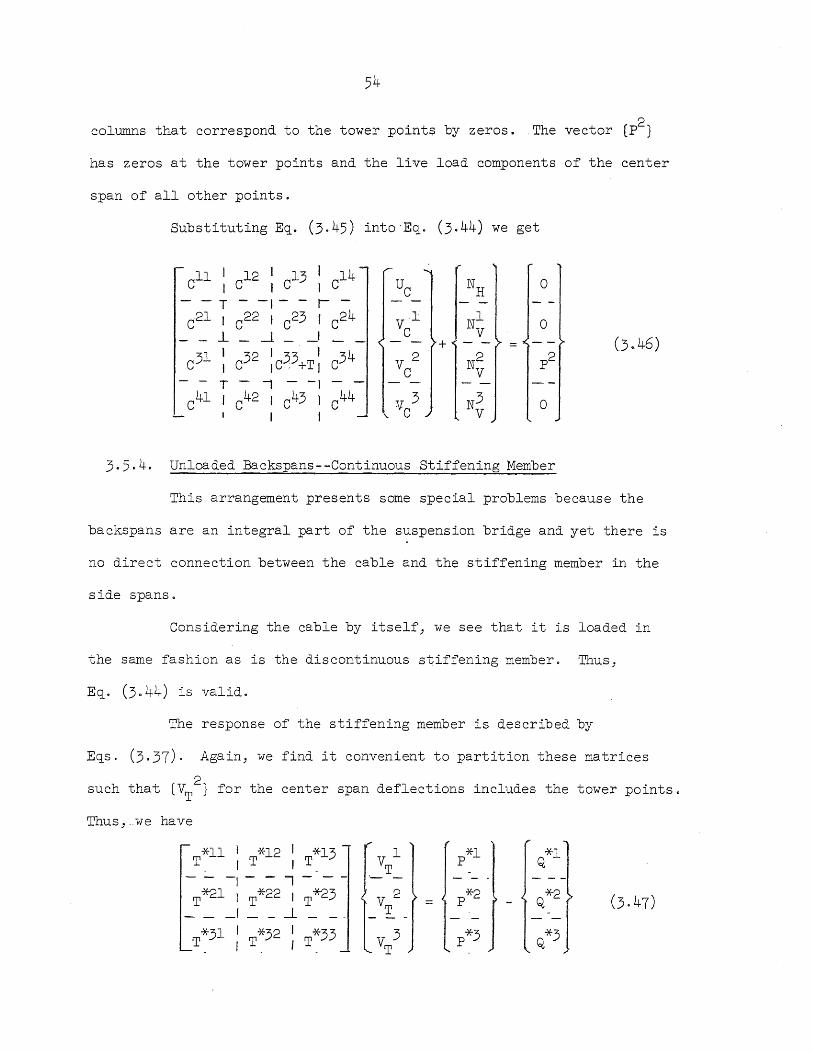
54
columns that correspond to the tower points by zeros. The vector (p2)
has zeros at the tower points and the live load components of the center
span of all other pOints.
Substituting Eq. (3.45) intoEq. (3.44) we get
11 1 12 I C13 I 14
Uc r-N~ 0 C 1 C I 1 C - - T - -,- - r- -C21
1 C22 1 C23 r C24 l Nl
0 Vc __ -1-_--1._ _I V (3.46)
c 31 : c32 :c3:3+T~ C34 V 2 +l~f p2 C
T - I - -I
C4l I C42 C43 I C44 3 0 , , Vc
3.5.4. Unloaded Backspans--Continuous Stiffening Member
This arrangement presents some special problems because the
backspans are an integral part of the suspension bridge and yet there is
no direct connection between the cable and the stiffening member in the
side spans.
Considering the cable by itself) we see that it is loaded in
the same fashion as is the discontinuous stiffening member. Thus)
Eq. (3.44) is valid.
The response of the stiffening member is described by
Eqs. (3.37). Again) we find it convenient to partition these matrices
2 such that (VT } for the center span deflections includes the tower points.
Thus) .. we have
*11 I *12 I
f~T~ ....
*13 *1 *1 T_ r T 1 T P Q
----1---' - --
T*21 I T*22 I T*23 V 2 *2 *2 (3.47)
[V:3 -
p Q - _ _I _ _ -1 _ __
*31 1 *32 I *33 *3 *3 T I T 1 T P Q
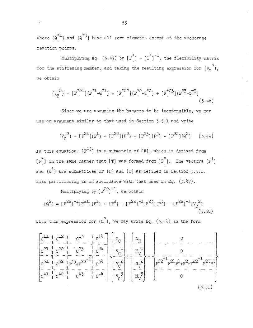
55
*1 *3 where [Q } and [Q } have all zero elements except at the anchorage
reaction points.
Multiplying Eq. (3.47) by [F*] = [T*]-l) the flexibility matrix
2 for the stiffening member) and taking the resulting expression for [VT
})
we obtain
Since we are assuming the hangers to be inextensible, we may
use an argument similar to that used in Section 3.5.1 and write
In this equation) [Fij ] is a submatrix of [FJ, which is derived from
* * i [F J in the same manner that [TJ was formed from [T J. The vectors [P }
and [Qi} are submatrices of [P} and (Q} as defined in Section 3.5.1.
This partitioning is in accordance with that uSed in Eq. (3.47).
Multiplying by [F22]-1) we obtain
[F22J-l[F21J(pl} + {p2} + [F22J-l[F23J(p3} _ [F22]-1(V 2} c
(3.50)
With this expression for (Q2}) we may write'Eq. (3.44) in the form
o
o
3.5.5. Final Equations
For the various arrangements of stiffened suspension bridges
considered in Sections 3.5.2,3.5.3 and 3.5.4, the final equations are
all of the same form. This can be seen by.examining,Eqs. (3.43), (3.46)
and (3.51). In all three cases, .we have an equation of the form
~
[A]{D} + (N} (P} (3.52)
where [A] is the modified [C] matrix in which the effect of the stiffening
member is included, (D} is the total displacement vector of the cable,
(N} is the matrix of nonlinear terms and (P} is a load vector which
includes zero elements for the first (n+l) elements and the live load
vector [P} or some modified version thereof for the last (n+l) elements.
In all cases, the only unknown quantities are the cable dis-
placement vectors (UC
} and (VC
}. Once these are known, the hanger loads
(Q} can be determined from Eq. (3041) or (3.44). The truss deflections
(VT} are also easily found from Eq. (3.39) and the truss reactions as
well as a' check on the hanger loads can then be found by using Eq. (3.37)
and Eq. (3.38). Knowing these quantities, we can determine the shears
and moments at all points of interest along the stiffening member.
3.60 Temperature Change
When a temperature change of 6t occurs, either separately or
in addition to the application of live load, the final strain energy of
the ith bar is
2 E.A.[e. n + (e·d-e. t )]
l l lL l l (3.53)
57
where
The coefficient of thermal expansion is represented by w.
Use of this strain energy expression instead of Eq. (3.5)
leads to the following cable equation:
r Ct J{-:~-} + {:~-) = {-:-} + {-::v1 The elements of [Ct ]) (NRt } and (NVt } are of the same form as those of
[C]) (NR} and (NV} of Eq. (3·32)) respectively, except that e id is
replaced by (eid-eit ). The vectors {PeR} and (PeV} have the following
elements:
~eht~d Kieithid PeRi 2
Lhd 2
Lid (i=l, ... ,n+l)
Khehtrhd K.e·tr· d l l l
PeVi = 2 2 Lhd Lid
These terms can be thought of as equivalent loads that if
applied would produce the displacements that are attributable to tempera-
ture change.
Actually, Eq. (3.55) is a general form of the cable equation.
When 6t = 0, this equation reduces to Eq. (3.32).
When the cable is part of a suspension bridge) a positive
temperature change will produce smaller displacements than would occur
for a simple cable subjected to the same temperature change. This is
true because as the cable displaces as a result of temperature change,
the stiffening member also deflects and relieves the cable of some
load that it originally carried.
For the present, consider only the case of loaded backspans
without hanger elongations. For the cable, we may write
tCtl~ l ~t ~1 C 21 I C 22 tit _
where PeVi = 0i PeVi represents the amount that the cable is unloaded
and the truss is loaded as a result of temperature change. For the
truss
Substituting Eq. (3.58) into Eq. (3.57), we obtain the following suspen-
sion bridge equation:
Equation (3.59) is of the same form as Eq. (3.52). The con-
tinuity characteristics of the stiffening member are reflected in [T].
An approach similar to the above leads to the essential relations for
unloaded backspans for both continuous and discontinuous stiffening
members.
The subject of hanger elongations, including the effect of
temperature change on the hangers, is discussed in Section 3.7.
59
3.7. Hanger Elongations
Consider first the case in which temperature change for the
main cable is ignored and the backspans are loaded. E~uation (3.41)
correctly gives the relationship governing the cable response and
E~. (3.37b) is the corresponding expression for the entire truss.
In this case, however, E~o (3.39) is replaced by
Cl·£· VCl. + ( l l) + Wo6t.£.
'A~H i l ( i =2, . . . , £ -1; £ + 1, 0 0 • ,r -1 ; r+ 1, . . . , 0)
(3.60)
where £i is the original length of the ith hanger and (AHEH)i is the
cross-sectional area multiplied by the modulus of elasticity of the
ith hanger.
Using E~. (3.60) instead of E~. (3.39), we obtain the following
e~uation in place of E~. (3.40a):
1
1 0 .t22
£ 0
r 0
lOt I n2
0\0 ••
£ r 0
0 . . 0 0 t 2n
0 .... 0. 0 •• 0
• • • • 0
o . . . . 0
vCl 0 0
~2£2 P2 ~2
vC2 + (AE) +ill o 6t o £2 2
P £-1 ~£-l 0 0
P£+l Cl£+l
r Pr-l Clr - l 0 0
Pr+l Clr +l
Pn j i~ j 0 l 0 J (3.61)
The above can be written in a form .with. order (n-3) by extract-
ing the rows and columns corresponding to the support points. This leads to
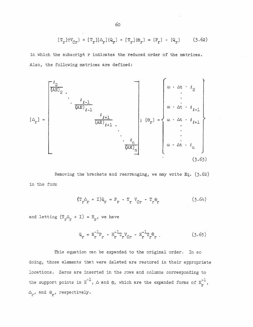
60
in which the subscript r indicates the reduced order of the matrices.
Also, the following matrices are defined:
£2 W· .6t £2 (AE) 2 .
££-1
(AE) £-1 W· .6t ££-1
[.6 ] ££+1
(8 } .6t ££+1 CAE) £+1 w o
r r
£ n .6t £ (AE)
W· n
n
(3863)
Removing the brackets and rearranging, we may write Eq. (3.62)
in the form
(T.6 + I)Q = P T V T Q r r r r r Cr - rOr
and letting (T.6 + I) r r
H , we have r
This equation can be expanded to the original order. In so
doing, those elements that were deleted are restored in their appropriate
locations. Zeros are inserted in the rows and columns corresponding to
-1 -1 the support points in H , . .6 and 8, which are the expanded forms of H )
r
.6 , and 8 ) respectively. r r
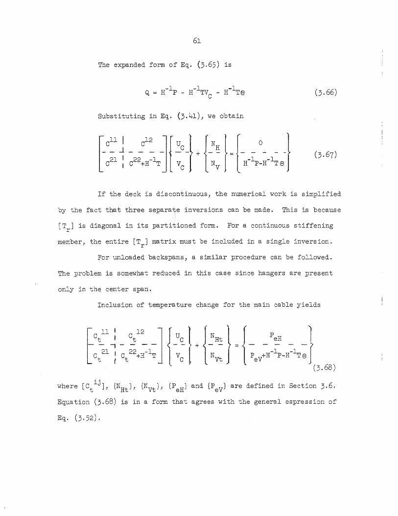
61
The expanded form of Eq. (3.65) is
Q
Substituting inEq. (3.41), we obtain
If the deck is discontinuous, the numerical work is simplified
by the fact that three separa~e inversions can be made. This is because
[T ] is diagonal in its partitioned form. For a coptinuous stiffening r
member, the entire [T ] matrix must be included in a single inversion. r
For unloaded backspans, a similar procedure can be followed.
The problem is somewhat reduced in this case since hangers are present
only in the center span.
Inclusion of temperature change for the main cable yields
where [CtijJ, (NRt } , (NVt } , (PeR} and (PeV} are defined in Section 3060
Equation (3068) is in a form that agrees with the general espression of
Eqo (3052).
62
3080 Newton-Raphson Method
The solution of Eq. (3.52) requires that we determine displace-
ments (D} that are caused by some given load (P}. However, because of
the nonlinearity, it is very difficult to solve for these displacements.
It is, however, quite easy to solve for the loads that would be required
to deform the structure by some designated displacements. This suggests
an iterative method that will enable us to solve Eq. (3052). This
method, commonly called the Newton-Raphson method, is discussed by
Livesley (1964). The Newton-Raphson method is a numerical scheme that
is commonly used to solve nonlinear equations. It will be described
here as it applies to the problem under study.
The behavior of a suspension bridge as it responds to loading
is represented schematically in two dimensions in Figure 10. The actual
system must, of course, be represented by hypersurfaces corresponding to
Eqo (3.52). Although for some loading conditions there will be certain
points on the bridge that do not reflect this load-displacement relation,
this will be the dominant behavior since the bridge becomes stiffer as
it deflects.
Equation (3.52) thus represents the load-displacement relation
ship that governs the behavior of the bridge as loading is applied to
some known configuration 0 From Figure 10, it can be seen that with the
origin at point d, the load-displacement relation is measured from the
dead load configuration. For this origin, the elements of the [A] matrix
of Eqo (3.52) that occur in matrix [C] and the elements of '(N} must be
calculated in terms of geometric parameters that are evaluated at the
dead load configuration. However, as was previously pointed out in
Section 3.203.3, the reference level can be any known configuration.
For instance, if we used the elevated reference axis with origin at 0,
Eq. (3.52) would still be valid. Here, however, the elements of
matrix [A] that are cable terms and the elements of {N}, are evaluated
at this known reference configuration. In any case, {P} refers to the
load vector "abovel! the load corresponding to the known configuration 0
The vector {D} refers to the displacement vector lIaboveT! this known
configuration. In Figure 10, ·Eq. (3.52) is written for two different
points on the curve; the subscript d or 0 signifies the appropriate
reference axes.
The application of the Newton-Raphson method to determine the
displacements {D} corresponding to the load vector {P} is illustrated
schematically in Figure 11 and summarized in Table 1. We trace the
development of Figure 11 as follows:
The total load (P} will be applied to the bridge in increments
of (LF}. Consider the first increment of (6P}. We start at the known
dead load configuration at which the total load vector (P} and the
corresponding live load displacement vector (D} are zero. Also, the
displacements for the first increment of load and the loads corresponding
to this set of displacements are initially zero. These are denoted by
....., I
(DO} and (PO} , respectively, in Figure 11. We now linearize about the
origin (the current known configuration, in this case the dead load
configuration) and determine the displacements (~l} corresponding to
the load vector (Pl
}, the residual loads, which in this case equals the
current load increment, (6P}. We do this by solving for (6Dl } from
Eq. (3.52) with the nonlinear part temporarily set equal to zero. We now
64
use the displacements, (Dl } = (6Dl }, and substitute back into the full
nonlinear form of Eg. (3.52) and obtain (PI}'. These are the loads that
would be necessary to keep the structure in equilibrium with the dis
placements (Dl }. Since (PI}' does not agree with the applied increment
of live load (~} we do not have the correct displacements. We now apply
a load vector equal to (P2} (in this case, negative loads as shown in
Figure 11), which are the amounts by which the equations were not
satisfied at (Dl }, or the new residual loads. Using these loads, 'we
find the displacements (6D2} by using the linear part of Eq. (3.52)
linearized about the point corresponding to the displacements, CDl
}.
The displacement vector, (6D2} , enables us to obtain (D2} = (Dl + 6D2}.
Using (D2
}, we can determine (P2 } , by substituting into the full nonlinear
form of Eq. (3.52). This enables us to get (P3
}, etc. The procedure
continues as tabulated in Table 1 until the applied increment of load and
the load vector as determined from the current displacements agree to any
desired degree of accuracy.
There is one important point to recognize. The curve as shown
in Figure 11 is a graphical portrayal of Eq. (3.52). As long as (P} and
(D) refer to the known configuration origin, the points along the curve
are represented by Eqo 13.52) only if the coefficients of these equations
are in terms of parameters evaluated at this known configuration. Thus,
whenever the (Po} I values are determined, ·Eq. (3.52) must be expressed l
in terms of the known configuration parameters. However, for each
linearization at some current {D}, Eq. (3.52) is used with coefficients
defined by parameters evaluated at this deflected position.

Once we have determined the correct deflections, (D}, for the
current load increment, (6P}, the deflected position becomes the new
known configuration. The reference origin can then be shifted to the
new known configuration as indicated in Figure 10, and,the next increment
of load is,:applied~,: This :proce1diJ.re is'·corttinued until the full live load
is on the structure. It was found that this incremental procedure was
necessary because in general, the correct representation involves
hyperplanes tangent to twisted hypersurfaces instead of the simplified
curve of Figure 10. When the load was applied all at once, in some cases
the procedure failed to converge.
40 ANALYSIS USING A CONTINUOUS STRUCTURAL SYSTEM
4010 Description of the Mathematical Model of the Structure and Outline of the Analysis
In the analysis using the discrete system of structural
elements, the departure from the real structure involves replacing the
continuous cable by a discrete analog. For the analysis using a con-
tinuous structural system, the departure from the actual structure
involves representing the stiffening member (which can be a discrete
system) and the hanger elements by continuous analogs.
For an actual suspension bridge, the stiffening member is
usually a truss. In such cases, the prime objection to replacing this
by a beam of equivalent bending stiffness is that the shear deformations
are ignored. In this study, this objection is partially removed by
replacing truss-type stiffening members with a Timoshenko beam [see
Langhaar (1962)J, which, ~lthough a continuous member, does provide for
the shear deformations that the real structure undergoes. As in the
discrete study, only vertical d.eflections of the stiffening member are
considered. Also, as in Chapter 3, stiffening members that are either
continuous or discontinuous at the tower points can be handledo
The hangers in actual suspension bridges are wire ropes that
hang at regular intervals from the main cable to support the roadway.
In the continuous study, these elements are replaced by an elastic sheet
that provides a continuous vertical connection between the stiffening
member and the cable 0 It will be seen that, in general, this replacement
has little effect on the final deflections, shears and moments of the
66
stiffening member. However, in considering local effects, such as the
stiffening member reactions at the towers, care must be exercised in
order to interpret the continuous results properly in terms of the real
structure.
As in the discrete study, the cable is considered free to
displace both vertically and horizontally. However, because of the
assumed continuous nature of the connection between the cable and stif
fening member throughout, it is more convenient to take the tower and
anchorage points to be fixed vertically for both cable and decko This
differs slightly from the discrete study where the vertical cable dis
placements at the tower and anchorage points are dependent upon the
stiffness of the support points even though the deck is fixed vertically.
The interconnection of the cable, saddle and tower is handled
as in the discrete case with the exception that vertical displacements
of the tower points are not allowedo The anchorage points are also
treated as in the discrete study with the additional specification that
the turn-down saddles displace horizontally and that the stiffness of the
saddle-support frame be infinite in order to inhibit vertical displace
ments of these points. As before, the large anchorage mass and the tower
foundations are considered to be rigid with regard to translation and
rotation,
The continuous model provides for consideration of hanger
elongations if desired, or the normal assumption of inextensible hangers
can be treated. As before, hanger inclinations are ignored. Also, as
in the discrete study, either loaded or unloaded backspans are allowed.
68
In the theory presented in this chapter, flexural stiffness of
the stiffening member is. assumed to be uniform in each span. This re
quirement can be relaxed, as is indicated in Section 4.9.
Once again, as in the conventional deflection theory, it is
assumed that the entire dead weight of the structure is uniformly dis
tributed horizontally. It is also assumed that the entire dead load is
supported by the cable, or that the stiffening member is unstressed at
mean temperature;-updex:cdead~·16ad.-·~·These a.ssumptions completely define
the dead load geometry of the system.
In this chapter, a formulation of the suspension bridge
problem as a continuous system is presentedo The nonlinear nature of
the problem again suggests use of a Newton-Raphson procedure 0 The
Newton-Raphson method as it is used here is discussed in Section 408.
For use in each linearization of the Newton-Raphson procedure,
general ~i~earized equations are developed in Section 4.5 for each case
being s-:'"J.iied. These equations are applicable for linearization about
any poi~-: i~ ~he loading sequence.
T~e two-point boundary-value problem is solved as a set of
initia:"-":&':'-..;.e p:-oblems. This procedure is discussed in Section 407.1
and t~e :~-:eg:-a-:ion procedure used in all solutions is presented in
Sectic:-.
:;u:::e:-ical difficulties are encountered that require special
treatmer.t. The method used in overcoming these difficulties is discussed
in Section 4.7020
4.2. Cable Equations
An element of the cable is shown in Figure 12 both in the dead
load, mean temperature position and in the final displaced position that
results from the application of live load and temperature change 0
For dead load alone and mean temperature, the curve formed
by the cable is described by
y = y(x) (4.1)
The x-y coordinate axes form a spatial system used to describe
the structure in its configuration at dead load and mean temperature.
If the point (x,y) on the cable at dead load and mean tempera
ture undergoes vertical and horizontal displacements of ~(x) and ;(x),
respectively, during the application of live load and temperature change,
then the final position of the cable may be described by
~ = ~(a) (402)
in which we have the following parametric expressions for a and ~g
a = x + ;(x)
~ = y+ ~(x)
The a-~ coordinate axes form a spatial coordinate system which
locates points of the structure in some deformed configuration.
Let Hd be the horizontal component of cable force that results
from the action of qVd and qHd' the vertical and horizontal components
of load that are applied to the cable at dead load and mean temperature.
Both of these loads are a function of x, the original horizontal
70
coordinate. For this condition of loading, the following differential
equations of equilibrium are applicable for the cable:
(4.4)
If the cable of a suspension bridge with vertical hangers is
considered, the load carried at dead load and mean temperature is
vertical only. In this case, Eqs. (404) reduce to
2 H ~ = -qVd
d dx2
Hd = constant
In order to make the formulation of the cable equations com-
pletely general, the horizontal components of load will be included.
Later, when these cable equations are applied to the suspension bridge
problem, those terms that drop out will be indicated.
When live load and temperature change are applied, additional
loads are imposed on the cable. For suspension bridge cables in which
the hangers are vertical and are assumed to remain vertical during
loading, there will be no horizontal component of load on the cable in
the final displaced position. However, in the numerical procedure used
in the continuous study, it is necessary to consider horizontal
components of load corresponding to some assumed set of displacements.
Thus, taking qv and qH as the total vertical and horizontal components
71
of load on the cable in the deformed position and H as the total hori-
zontal component of cable tension, we obtain the following equilibrium
equations for the cable:
dH dO: -q
H
-q V
(4.6)
In the above equations, the loads qv and qH are a function
of 0:, the horizontal coordinate for the deformed structure. The positive
directions for all quantities are those shown in Figure 12.
4.2.1. Equations for qv and qH
Equations (4.6) are the governing differential equations for
the cable. It is necessary to express these equations in terms of the
displacements that occur when the live load and temperature change are
d~ d2~ d dH . applied. This is accomplished by determining do: ) 2 ) an dO: In terms do:
of sand Tj, as functions of x. This leads to
dH do:
dH/· do: HI dx· dx = (l+s I)
where primes indicate differentiation with respect to x.
72
Thus, Eqso (406) become
-HI (l+~r) (4.8)
All differentiation is with respect to x, the original dead
load., -mean temperature horizontal coordinate axis. This is necessary
for the solution procedure that is used.
402.2. Equation for H
Equations(4.8) contain H, which is also dependent upon the
cable displacements ~ and~. A relationship for H in terms of these
displacements is developed in this section
222 Letting ds = dx + dy and Td be the tension in the cable at
dead load, we have
T 0 dx ____ T_d __ _
d ds .1 IJI + (~)
2
Or, we may write
As a result of the application of live load and temperature
change, there is a change of T1 in the cable tension. The final tension
T is then
T
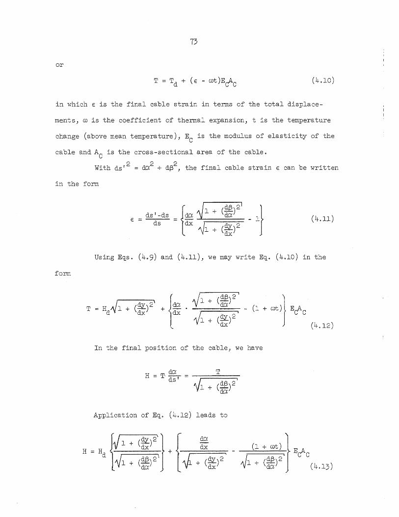
73
or
(4.10)
in which E is the final cable strain in terms of the total displace-
ments, w is the coefficient of thermal expansion, t is the temperature
change (above mean temperature), EC is the modulus of elasticity of the
cable and AC is the cross-sectional area of the cable.
With ds,2 = dO? + d(32, the final cable strain E can be written
in the form
form
E ds' -ds
ds - Jcl.O: 1l + (~l - lj - ldx -.&.~-;:::l =+:::::=:dy=2=-
(-) dx
Using Eqs. (4.9) and (4.11), we may write Eq. (4.10) in the
In the final position of the cable, we have
Application of Eqo (4012) leads to
(1 + wt) } E_A d(3 2' C;-C
~l + (da) (4.l3l
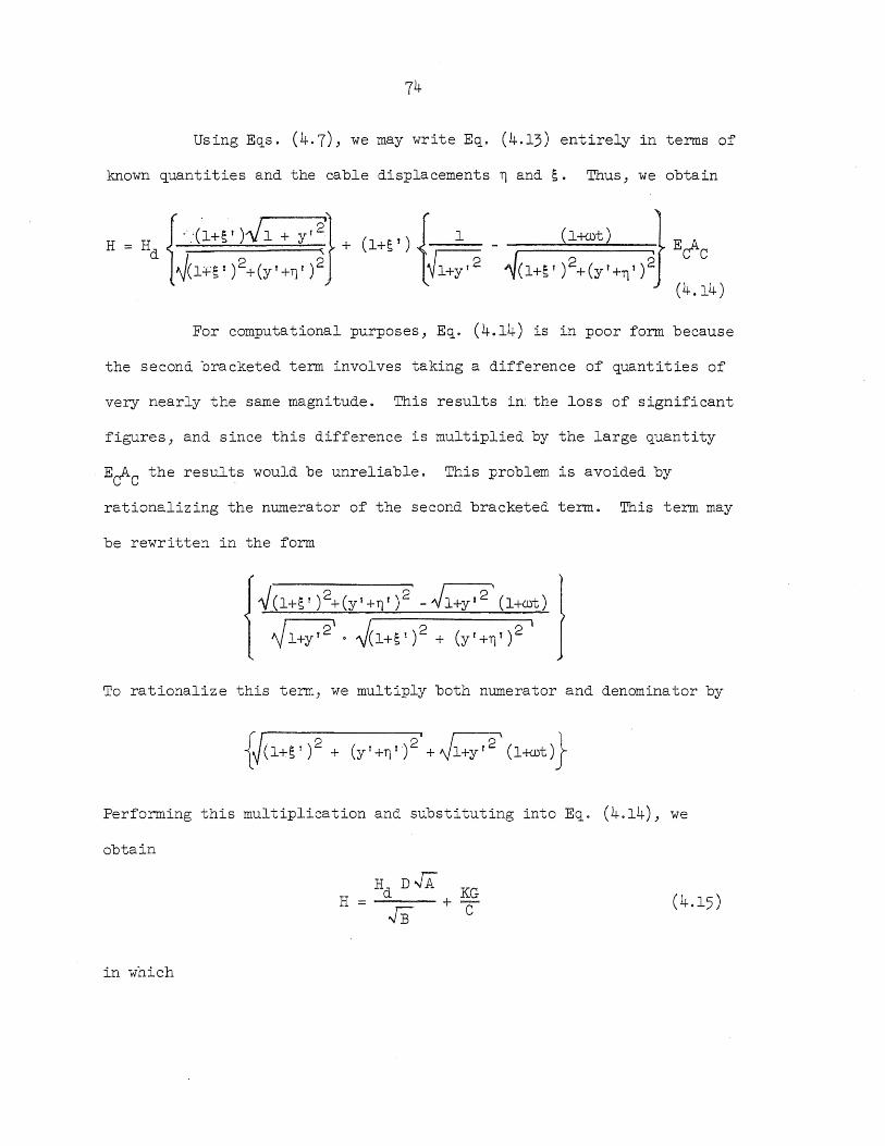
74
Using Eqs. (4.7), we may write Eq. (4.13) entirely in terms of
known quantities and the cable displacements ~ and~. Thus, we obtain
H
For computational purposes, Eq. (4.14) is in poor form because
the second bracketed term involves taking a difference of quantities of
very nearly the same magnitude. This results in; the loss of significant
figures, and since this difference is multiplied by the large quantity
E~C the results would be unreliable. This problem is avoided by
rationalizing the numerator of the second bracketed term. This term may
be rewritten in the form
To rationalize this term, we multiply both numerator and denominator by
Performing this multiplication and substituting into Eq. (4.14), we
obtain
H (4.15)
in which
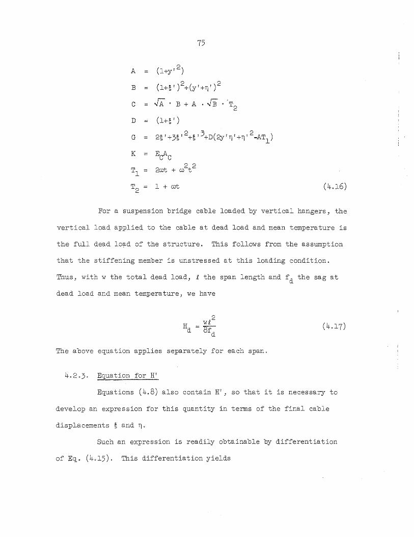
75
A (1+yf2)
B 2 2 (l+S') +(y'+Tj')
c JA 0 B + A • .JB . 'T2
D (l+S! )
G
K
1 + wt (4.16)
For a suspension bridge cable loaded by vertical hangers, the
vertical load applied to the cable at dead load and mean temperature is
the full dead lo?d of the structure. This follows from the assumption
that the stiffening member is unstressed at this loading condition.
Thus, with w the total dead load, £ the span length and fd the sag at
dead load and mean temperature, we have
The above equation applies separately for each spano
4.2.3. Equation for HI
Equations (4.8) also contain HI) so that it is necessary to
develop an expression for this quantity in terms of the final cable
displacements sand Tj.
Such an expression is readily obtainable by differentiation
of Eqo (4015)0 This differentiation yields
HI
HdDA.' KS + + --
2 ~AB C (4.18)
in which
p
Q
E (y! +Tj ! )
F 2DE
S D ( 2y II Tj ! -A ! T ) 1
R = AlB + Ai .JB T 2 JA 2
(4.19)
For a suspension bridge with vertical hangers) qHd 0) and
thus Hei O.
403. Equations of Stiffening Member
Two different types of stiffening members will be studied. The
first to be treated is the conventional Bernoulli-Euler beam in which
only deformations due to flexure are considered. Secondly) a Timoshenko
beam will be studied. Here) in addition to flexural deformations) there
exists a provision for including the effects of shear deformation. This
feature permits investigation of the suspension bridge without ignoring
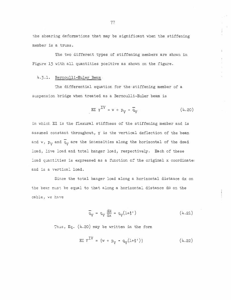
77
the shearing deformations that may be significant when the stiffening
member is a truss.
The two different types of stiffening members are shown in
Figure 13 with all quantities positive as shown on the figure 0
4.3.1. Bernoulli~Euler Beam-
The differential equation for the·stiffening member of a
suspension bridge when treated as a Bernoulli-Euler beam is
EI YIV
= w + PV - qv (4.20)
in which EI is the flexural stiffness of the stiffening member and is
assumed constant throughout, y is the vertical deflection of the beam
and w, Pv and qvare the intensities along the horizontal of the dead
load, ~ive load and total hanger load, respectively. Each of these
load ~uantities is expressed as a function of the original x coordinate:
and is a vertical load.
Since the total hanger load along a horizontal distance dx on
the bea~ ~us~ be equal to that along a horizontal distance da on the
cable, ~e have
(4.21)
~h~s, Eq. (4.20) may be written in the form
(4.22)
4.3.2. '. Timbshenko Beam
For the Timoshenko beam, it is assumed that in addition to
the deformations caused by bending, there are shearing deformations.
The shear slope 5 may be expressed as
(4.23)
in which V is the shear force and k is a constant which depends on the s
cross section and materials of the stiffening member. The determination
of k is discussed belowo s
If Y is the total deflection, then the slope that is caused by
bending is (y'-5) and the curvature due to bending is (yll_5'). Thus,
the differential equation for the Tirnoshenko beam may be written as
ElY" -M + EI 0 I (4.24)
where M is the bending moment of the stiffening member. In Eq. (4.24),
(4.25 )
and applying Eqo (4021), we obtain
(4.26)
The Timoshenko beam constant, k , depends on the character of s
the stiffening member. It can be determined quite easily by determining
the slope that is caused by a given shear force applied to an element of
the stiffening member. The actual value of k then follows from s
Eq. (4.23). Truss-type stiffening members are the only kind for which
shear deformations are of any consequence. Stiffening trusses for;
79
suspension brRdges are generally Warren trusses with vertic~ls.
Timoshenko and Gere (1961) show that for such trusses
k s
1
where Ad is the cross-sectional area of the diagonal) Ed is the modulus
of elasticity for the diagonal and ~ is the angle that the diagonal makes
with the vertical.
4040 Suspension Bridge Equations
In Sections 4.2 and 403) the basic differential equations of
the cable and stiffening member have been developed. In this section,
these equations are grouped into sets that are applicable for each type
of suspension bridge that is to be considered.
Here and in subsequent sections) it will be assumed that only
,a vertical component of load is applied to the cable at dead load and
mean temperature (ioee) qVd = wand qHd = 0). All live loads are assumed
to be applied vertically.
404.10 Unstiffened Suspension Bridge (CASE A)
For the unstiffened suspension bridge, the stiffening member
is extremely flexible; it functions merely as a loading platform. It
is assumed that this platform transfers the applied live load to the
hanger sheet. Thus, in this case) the analysis reduces to that of a
loaded cable that is subjected to some initial dead load prior to the
application of live load.
80
Using the notations for load terms that have already been
introduced and Eqo (4.21), we may write the following vertical equilibrium
equation for the cable~
(4.28)
For horizontal equilibrium of the cable, we have
(4.29)
where PH is the horizontal component of live load that is applied to the
cable and is taken as a function of a. This is done as a matter of
convenience since PH enters only as a residual load in the numerical
procedure and it does not correspond to an applied live load. If we
were dealing with a cable in which horizontal loads were applied, then
greater care would have to be exercised.
Equations (4028) and (4029) are the basis for the determina
tion of the displacements ~ and ~.
4o~,2. S~:f:ened Suspension Bridge
C~~i~e the unstiffened suspension bridge, the stiffened bridge
has a :~-":3::: :::- girder with some flexural stiffness. Here, the stiffen
ing me~~e:- c::s to alter significantly the magnitude and distribution
of the :"':-;e loai that is transferred to the cable. Therefore, the
stiffeni~g ~e~ber must carry some of the live load itself through con
ventional bearr behavior as it deflects under the applied live load and
temperature change.
81
4.4.2.1. Stiffened Bridge Without Hanger Elongations
In this case, it is assumed that the hanger sheet is inexten-
sible. That is, the vertical deflection of the stiffening member is
equal to the vertical displacement of the cable at all points. Then,
(4.30)
4.4.2.1.1. Bernoulli-Euler Beam as Stiffening Member (CASE :E3)
Recalling Eq. (4.22) and including the relation given by
Eq. (4.30), we obtain
This differential equation expresses the vertical equilibirum
of the structure. Along with Eq. (4.29), which defines the horizontal
equilibrium of the cable, it provides the necessary equations for
determining the displacements which define the response of the structure.
4.4.2.1.2. Timoshenko Beam as Stiffening Member (CASE C)
Equation (4.24) applies in this case; however, since there are
no hanger elongations, Eq. (4.30) is also valid. This leads to
11 II - 0 I -M ( 4.32) - EI
Substituting Eq. (4.26) for Of into Eq. (4.32), we find
M nil + k (w + P _ q (1+1: f )} 'I S V V s = - EI
From the equilibrium of a beam element, it can be seen that
(4.34)
82
Equation (4.34) expresses the vertical equilibrium of the
structure and Eq. (4.33) relates the curvatures of the stiffening member
to the moment. These equations together with the equation of horizontal
equilibrium of the cable [Eq. (4.29)J furnish the required equations for
the determination of the displacements ~ and s. Once again, knowing
these displacements all other quantities of interest can be found.
4.4.2.2. Stiffened Bridge With Hanger Elongations
If the extensions of the continuous hanger sheet connecting
the cable and the stiffening member are taken into account, then the
vertical deflection of the deck is no longer equal to the vertical cable
displacement.
Taking y to be the vertical deflection of the stiffening
member, we may write
T
where ~ is the stiffness of the hanger sheet, which varies along the
length of the structure. The net load (qv - w) is the load which the
hanger sheet transfers to the cable as a result of the live load and
temperature change 0 The last term in the above equation reflects the
effect of temperature change on the hanger length. The quantity Lh is
the dead load;··mean temperature hanger length, (J) is the coefficient of
thermal expansion, and t is the temperature difference.
Making use of Eqo (4021), we may express Eq. (4.35) in the form
4.4.2.2.1. Bernoulli-Euler Beam as Stiffening Member (CASE D)
For this case, Eq. (4.22) correctly states the condition for
vertical equilibrium of the structure. Equation (4.36) describes the
condition of compatibility between the cable and the stiffening member.
These two equations and Eq. (4.29), which states the condition of hori-
zontal equilibrium for the cable, supply the needed relations to solve
for the displacements ~, y and ~.
4.4.2.2.2. Timoshenko Beam as Stiffening Member (CASE E)
For this arrangement, Eq. (4.34) gives the relationship that
must be satisfied for vertical equilibrium of the structure.
Substituting Eq. (4.26) into Eq. (4.24), we obtain the following
equation which gives the condition that must be satisfied by the curva-
tures of the stiffen~ng member:
These two equations combined with Eq. (4.36) and Eq. (4.29)
supply the relations that are required to find the displacements ~, ~ and
T. With these displacement' quantities known, all other quantities of
interest are determinable.
4.4.3. Comments on Format of Equations
A careful examination of the derivations of the equations in
the preceding sections reveals that any substitution that would lead to
differentiation of the quantity qv has been avoided. In this way, a set
of equations has been obtained in which the highest derivatives present
{:II IV II II are among s , T)._. , ~ and M in the cases where hanger elongations are
84
IV· ignored" and among S Ii" Y Tj 11" ,", and M" in cases where hanger elonga-
tions are included.
Had other substitutions been employed" higher-order systems
would have been obtained. It would then be necessary to provide
equations and boundary conditions for higher-order derivatives. Such
equations would become very complex and the required boundary conditions
would be difficult to interpret.
The procedure used in deriving the equations leads to a system
of lowest order without introducing subsidiary variables. The resulting
equations are solved by the methods discussed in subsequent sections.
405. Linearized Equations
In the previous section" several suspension bridge arrange-
ments have been considered. For each case presented" a set of equations
has been assembled forming the basis for a solution for the final dis-
placements. All of these equations contain either qv or qH" which are
defined by Eqsc (408)0 These equations are nonlinear, and consequently
all of the expressions developed in Section 4.4 are also nonlinear.
Thus, for each bridge arrangeme"nt described in the previous section" the
final displacements are obtained by solving a set of nonlinear dif-
ferential equationsc
The nonlinear character of these equations requires a special
technique for solution 0 The procedure employed is the Newton-Raphson
method" which is discussed fully in Section 408. An important feature
of this method is that the live load is applied in increments. For each
increment, a series of linearizations lead to the correct solution to
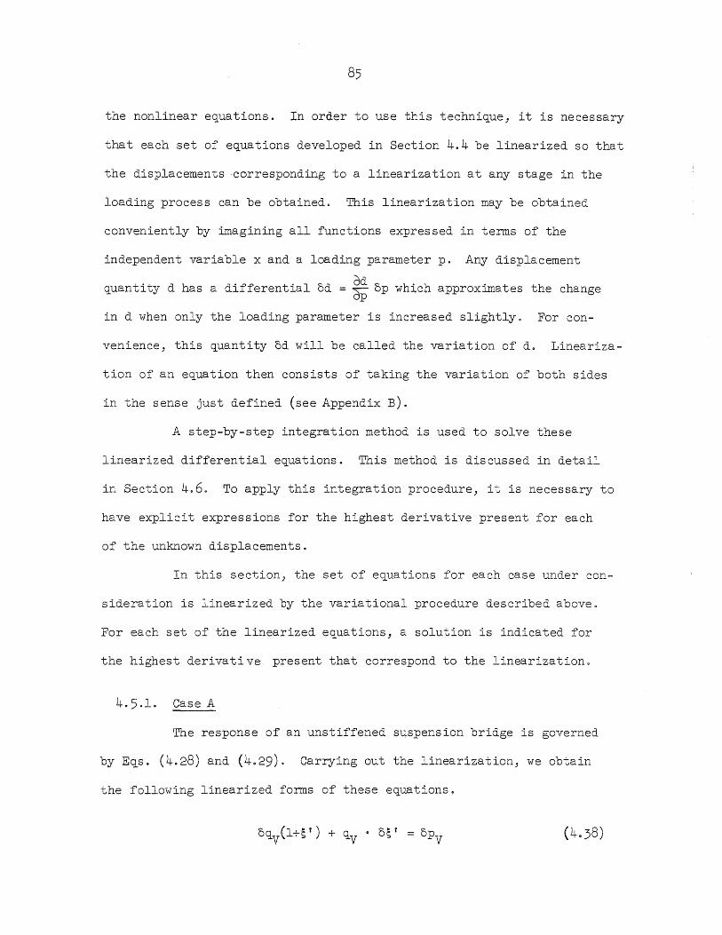
the nonlinear equations. In order to use this technique} it is necessary
that each set of equations developed in Section 4.4 be linearized so that
the displacements ·corresponding to a linearization at any stage in the
loading process can be obtained. This linearization may be obtained
conveniently by imagining all functions expressed in terms of the
independent variable x and a loading parameter po Any displacement
quantity d has a differential 6d = ~ 6p wh~ch approximates the change
in d when only the loading parameter is increased slightly. For con-
venience} this quantity 6d will be called the variation of d. Lineariza-
tion of an equation then consists of taking the variation of both sides
in the sense just defined (see Appendix B).
A step-by-step integration method is used to solve these
linearized differential equations. This method is discussed in detail
in Section 4.6. To apply this integration procedure} it is necessary to
have explicit expressions for the highest derivative present for each
of the unknown displacements.
In this section, the set of equations for each case under con-
sideration is linearized by the variational procedure described above,
For each set of the linearized equations} a solution is indicated for
the highest derivative present that correspond to the linearization.
4.5.1. Case A
The response of an unstiffened suspension bridge is governed
by Eqs. (4.28) and (4.29). Carrying out the linearization, we obtain
the following linearized forms of these equations~
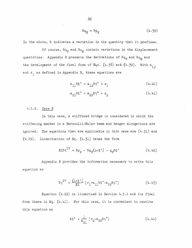
86
In the above) 0 indicates a variation in the quantity that it prefixes.
Of course, oqv and oqH contain variations in the displacement
quantities. Appendix B presents the derivations of oqv and oqH and
the development of the final form of Eqs. (4.38) and (4039)0
and r. as defined in Appendix B) these equations are l
a osll+a OTJII 11 12
405.20 Case B
With a .. lJ
(4040 )
(4.41)
In this case, a stiffened bridge is considered in which the
stiffening member is a Bernoulli-Euler beam and hanger elongations are
ignoredo The equations that are applicable in this case are (4.31) and
(4029)0 Linearization of Eqo (4.31) takes the form
(4042)
Appendix B provides the information necessary to write this
equation as
(4.43 )
Equation (4.29) is linearized in Section 40501 and its final
form there is Eq. (4041)0 For this case) it is convenient to rewrite
this equation as
(4.44)
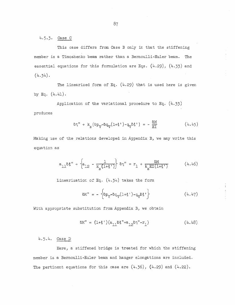
87 I
4.5.3. Case C
This case differs from Case B only in that the stiffening
member is a Timoshenko beam rather than a Bernoulli-Euler beam. The
essential equations for this formulation are Eqs. (4.29)) (4.33) and
(4.34) .
The linearized form of Eq. (4.29) that is used here is given
by Eq. (4.41).
Application of the variational procedure to Eq. (4.33)
produces
(4.45)
Making use of the relations developed in Appendix B, we may write this
equation as
(4.46)
Linearization of Eqo (4.34) takes the form
With appropriate substitution from Appendix B, we obtain
oM" (l+~r)(a 5~!I+a oTjii_r) 11 12 1
Here) a stiffened bridge is treated for which the stiffening
member is a Bernoulli-Euler beam and hanger elongations are included.
The pertinent equations for this case are (4.36), (4.29) and (4022).
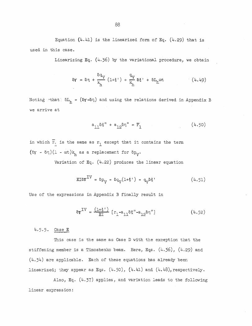
88
Equation (4.41) is the linearized form of Eq. (4.29) that is
used in this case.
Linearizing Eqo (4.36) by the variational procedure, we obtain
or (4.49)
(or-o~) and using the relations derived in Appendix B
we arrive at
a OSH + a O~" - F 11 12 - 1
in which r l is the same as r l except that it contains the term
(oy - o~)(l - illt)~ as a replacement for oPV.
Variation of Eq. (4.22) produces the linear equation
Use of the expressions in Appendix B finally result in
(4.50)
This case is the same as Case D with the exception that the
stiffening member is a Timoshenko beam. Here, Egs. (4.36), (4.29) and
(4.34) are applicable. Each of these equations has already been
linearized; they appear as Eqsp (4.50), (4.41) and (4.48),respectively.
Also, Eg. (4037) applies, and variation leads to the following
linear expression~
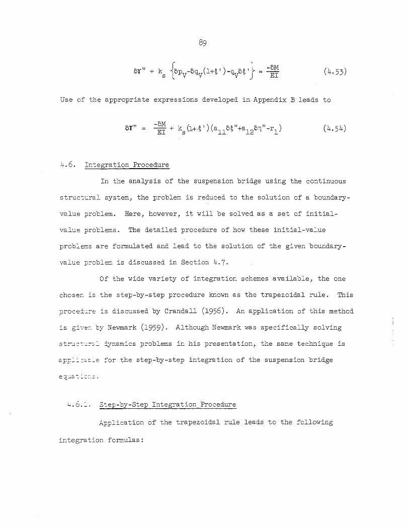
Use of the appropriate expressions developed in Appendix B leads to
(4.54 )
4.6. Integration Procedure
In the analysis of the suspension bridge using the continuous
structural system, the problem is reduced to the solution of a boundary-
value problem. Here, however, it will be solved as a set of initial-
value problems. The detailed procedure of how these initial-value
problems are formulated and lead to the solution of the given boundary-
value problem is discussed in Section 4.7.
Of the wide variety of integration schemes available, the one
choser. is the step-by-step procedure known as the trapezoidal rule. This
procej .. ~re is discussed by Crandall (1956). An application of this method
is gi';e:-. by Newmark (1959). Although Newmark was specifically solving
st:r-.l2-:·~r:::.2.. iynamics problems in his presentation, the same technique is
app:~2~~c':'e ~or the step-by-step integration of the suspension bridge
4.6.2... Step-by-Step Integration Procedure
Application of the trapezoidal rule leads to the following
integration formulas:
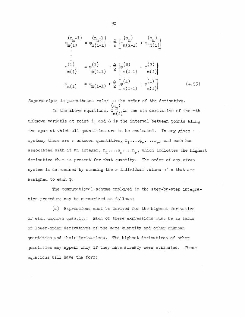
(1) (1) + /', r (2) (2) J cP = cP / . 2"CP + cP l1!-{t) ... til(i-l) m (i-l) m(i)
CPm(i) = cp + ~ [cp ( 1 ) + cp ( 1) ]
m(i-l) 2 m(i-l) m(i) . (4.55)
Superscripts in parentheses refer to the order of the derivative. (n )
In the above equations, CPm(i)iS the nth derivative of the mth
unknown variable at point i, and 6 is the interval between points along
the span at which all quantities are to be evaluated. In any given
system, there are r unknown quantities, cpl •... cp •••• cp , and each has m r
associated with it an integer, nl .... nm .... nr , which indicates the highest
derivative that is present for that quantity. The order of any given
system is determined by summing the r individual values of n that are
assigned to each cpo
The computational scheme employed in the step-by-step integra-
tion procedure may be summarized as follows:
(a) Expressions must be derived for the highest derivative
of each unknown quantity. Each of these expressions. must be in terms
of lower-order derivatives of the same quantity and other unknown
quantities and their derivatives. The highest derivatives of other
quantities may appear only if they have already been evaluated. These
equations will have the form:
91
(nl ) (nl-l)
CPli f(CPli'···'
(0) (~-l) (0) (nr-l) (0) CPl . ; .... ; cp ., ••• , cP .; ••• ; cP ., ••• , cP . ) l ml ml rl rl
(I1n) (nl)
CPmi f(CPli' ... , (0) (Dm-l) (0)
(4056)
(b) At the initial point (i=l), values are assigned to all
quantities and their derivatives except for the r highest derivatives.
These assignments are made on the basis of specified boundary conditions
at the initial point or are made arbitrarily. Application of Eqs. (4.56)
yields the corresponding values of the highest derivatives at the initial
point.
Thus, all the values are known at i=l and it is possible to
proceed to the point i=2 at an interval L along the structure. Or, in
general, once all values are known at some point (i-l) we proceed to
point i.
(c) At point i, it is convenient to assume at first that the
highest derivative of each unknown quantity is equal to the value at the
preceding point (i-l). Thus
(~) cP
mi (m=l, .. ,r)
(d) With this assumption, all lower-order derivatives may be
determined from Eqs. (4.55). These lower derivatives are then substi-
tuted in Eqs. (4056) and the resulting r highest derivatives are
determined.
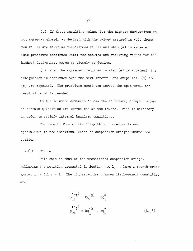
92
(e) If these resulting values for the highest derivatives do
not agree as closely as desired with the values assumed in (c), these
new values are taken as the assumed values and step (d) is repeated.
This procedure continues until the assumed and resulting values for the
highest derivatives agree as closely as desired.
(f) When the agreement re~uired in step (e) is attained, the
integration is continued over the next interval and steps (c), (d) and
(e) are repeated. The procedure continues across the span until the
terminal point is reached.
As the solution advances across the structure, abrupt changes
in certain quantities are introduced at the towers. This is necessary
in order to satisfY internal boundary conditions.
The general form of the integration procedure is now
specialized to the individual cases of suspension bridges introduced
earlier.
4.6.2. Case A
Ttis case is that of the unstiffened suspension bridge.
Followi~g ~te ~otation presented in Section 4.6.1, we have a fourth-order
syster:: -i..- " •• ::::::::: r = 2. The highest-order unknown displacement ~uantities
are
(nl ) 0~(2) II
CPli = o~. i 1.
(n2 ) 011(2) "
CP2i = 011. (4.58) i 1.
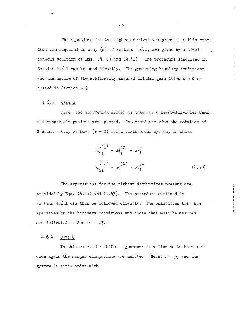
93
The equations for the highest derivatives present in this case)
that are required in step (a) of Section 4.6.1) are given by a simul-
taneous solution of Eqs. (4.40) and (4.41). The procedure discussed in
Section 4.6.1 can be used directly. The governing boundary conditions
and the nature of the arbitrarily assumed initial quantities are dis-
cussed in Section 4.7.
4.6.3. Case B
Here) the stiffening member is taken as a Bernoulli-Euler beam
and hanger elongations are ignored. In accordance with the notation of
Section 4.6.1) we have (r = 2) for a sixth-order system) in which
(nl) 5~(2) II
~li = 5~. i l
(n2) (4) 5 IV (4.59) ~2i = p~ = ~i
The expressions for the highest derivatives present are
provided by Eqs. (4.44) and (4.43). The procedure outlined in
Section 4.6.1 can thus be followed directly. The quantities that are
specified by the boundary conditions and those that must be assumed
are indicated in Section 4.7.
4.6.4. Case C
In this case) the stiffening member is a Timoshenko beam and
once again the hanger elongations are omitted. Here) r = 3) and the
system is sixth order with
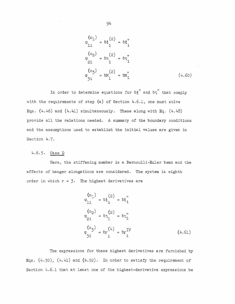
94
(nl) c;(2) " CPli = = cs.
i l
(n2) (2) JI
cp CT) = cT). 2i i l
(n3) (2) " CP3i = cM = cM. (4.60)
i l
" Ii In order to detennine equations for as and aT) that comply
with the requirements of step (a) of Section 4.6.1, one must solve
Eqs. (4.46) and (4.41) simultaneously. These along withEq. (4.48)
provide all the relations needed. A summary of the boundary conditions
and the assumptions used to establish the initial values are given in
Section 4.7.
4.6.5. Case D
Here, the stiffening member is a Bernoulli-Euler beam and the
effects of hanger elongations are considered. The system is eighth
order in which r = 3. The highest derivatives are
(nl ) (2) 11
CPli = cs. = c;i l
(n2) (2) "
CP2i cT). cT). l l
(n3
) (4) CyIV (4.61) cP = cy 3i i i
The expressions for these highest derivatives are furnished by
Eqs. (4.50), (4.41) and (4.52). In order to satisfY the requirement of
Section 4.6.1 that at least one of the highest-derivative expressions be
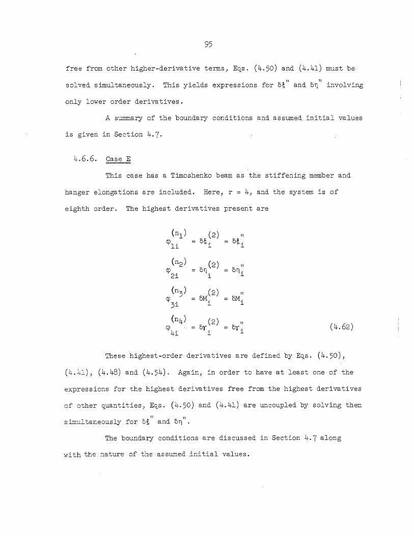
95
free from other higher-derivative terms, Eqs. (4.50) and (4.41) must be
solved simultaneously. II " This yields expressions for o~ and o~ involving
only lower order derivatives.
A summary of the boundary conditions and assumed initial values
is given in Section 4.7.
4.6.6. Case E
This case has a Timoshenko beam as the stiffening member and
hanger elongations are included. Here, r = 4, and the system is of
eighth order. The highest derivatives present are
(nl ) 0~~2) II
CPli = o~. l l
(n2) o (2) " CP2i ~. o~.
l l
(n3
) OM~2) " CP3i
oM. l l
(n4) (2) " (4.62) CP4i or. or i
l
These highest-order derivatives are defined by Egs. (4.50),
(4.41), (4.48) and (4.54). Again, in order to have at least one of the
expressions for the highest derivatives free from the highest derivatives
of other quantities, Eqs. (4.50) and (4.41) are uncoupled by solving them
" simultaneously for os I' and o~ .
The boundary conditions are discussed in Section 4.7 along
wi th the nature of the 'as'sumed ,initial va,lues.
4.7. Linear Solution
In the preceding sections, the linear equations and the inte
gration technique to be used in solving these equations have been
developed. We are now in a position to determine the linear solution
corresponding to some applied live load and temperature change.
4.7.1. Single-Span Structure
In this section, the discussion will be restricted to a single
span bridge. The essential departures from this procedure when three
span structures are considered will be discussed in Section 4.7.3.
At the initial point for the marching solution, certain
quantities are fixed by the boundary conditions, and the highest deriva
tives present are determined by the procedures outlined in Section 4.6.
Certain other values at the initial point must be assumed. For a system
of order 2j, j quantities must be assumed at the initial point, and
j boundary conditions must be satisfied at the terminal point.
In general, any set of j, assumed initial values will not lead
to a solution that satisfies the j terminal boundary conditions.
Instead, j boundary quantities are obtained at the terminal point that
do not satisfy the boundary conditions. The correct solution will
correspond to some other set of initial values that produce boundary
quantities satisfying the terminal boundary conditions. This correct
solution is determined as follows.
The solution of the two-point boundary-value problem as a set
of initial-value problems is central to the method employed. One
particular solution and j independent homogeneous solutions are carried
simultaneously. The true solution at any point is the sum of the
97
particular solution and some linear combination of the j homogeneous
solutions. Each of the (j+l) initial-value problems is solved
numerically as a marching problem using the integration procedures of
Section 4.6. The particular solution inc~udes the load for this
linearization, whereas the homogeneous solutions have no load.
For each solution, a set of j initial values must be assumed.
For the £th solution, the initial values are designated by the vector
(gi} in which the element gik (k=l, ... ,j) represents the kth initial
value. The particular solution corresponds to i=O and the j homogeneous
solutions are indicated by i=l, ... ,j. For convenience, the assumed
initial values for the particular solution are all taken to be zero,
and a set of orthogonal unit vectors are taken as the initial values
for the homogeneous solutions. In vector form, these initial-value
assumptions are
o o o
l ~ J o gj~=lj (4.63)
These initial values lead to a particular solution and j
independent homogeneous solutions which are designated by sO) sl'o .. ,Sj'
respectively. Each of-these solutions will have j terminal boundary
~uantities. For the ith solution, the terminal values are represented
by the vector (b i } with the element b ik (k=l, ... ,j) specifYing the kth
boundary quantity. In vector form, these boundary quantities can be
written as
(b } o
b .. lJ
,
btl
b£2
(b £}
b ££
b£j
, (b j}
b .. JJ
(4.64)
If the boundary quantities needed to satisfy the terminal
boundary conditions are given by the vector (b},with elements bk (k=l,
... ,j), then the particular solution and the j homogeneous solutions
must be combined such that these boundary values are obtained. This is
done as follows:
~ (b o} + L C £ (b £ }
£=1
(b}
The solution of this set of simultaneous algebraic equations
yields C£ (£=l, ... ,j) and these quantities designate how the homogeneous
solutions must be combined with the particular solution to produce the
correct solution' for this linearization. Expressing the final solution
as s) we have
s (4.66) £=1
99
The correct initial values for the final solution (g} would be
(g}
J
(gO) + L C £ (g i )
£=1
Since all solutions are linear, all quantities relating to the
final solution are obtained by a linear combination of the corresponding
quantities for each individual solution. One such quantity of special
interest is the variation in the horizontal component of cable tension.
Representing this quantity at point i for the final solution as oH. and l
those of the individual solutions as OHit (t=O,l, ... ,j), we have
oR. l
(4.68)
For a single-span structure, the boundary conditions and
the initial-value assumptions are listed in Tables 2 through 6 for the
cases being considered. For fixed supports, the entries in the tables
are easily verified; however, the case of flexible supports requires
some discussion.
Consider the current point of linearization. At this point
of linearization, horizontal equilibrium will not necessarily be satis-
fied at the support points. Let 6H represent the difference between the
horizontal component of cable force at the initial point due to live
load and temperature change and the horizontal component of reaction.
Indicating the initial point by the subscript 1, and referring to
Figure 14, we have
100
6H = (H -H ) - ~ ~ 1 d I-or (4.69)
where HI is the total horizontal component of cable force at the initial
point corresponding to the displacements of the current point of lineari-
zation, Sl is the horizontal displacement of the initial point corre
sponding to the current point of linearization and KT is the horizontal
* stiffness of the support point. In determining HI' the full nonlinear
expression is used [Eq. (4.15)].
For., the,corre.ct:;displacements, 6H must vanish. Thus, for the
next linearization, we want
or (4·70)
In the above, OHI is the required change in HI for this
linearization and o~l is the corresponding change in the horizontal dis-
placement of the support point. For convenience, this required change
can be taken in two parts, -6H and KT OSlo For the particular solution,
-6H
and for the homogeneous solutions
* In the continuous study, the flexural stiffness of the tower is taken to be the same regardless of the load on the tower. The discrete study includes a feature for treating the variable stiffness of the tower as the axial load changes. However, it was found that the
" change. in : stiffness was v.ery small as the loading was increased. Moreover, the bridge response was found to be insensitive to changes in stiffness. For these reasons, the tower stiffness is taken to be constant in the continuous study.
101
, (.f =1, ••. ,j ) (4·72)
Applying the expression for 5R from Appendix B at the initial
point for each solution, we have
( I=O, 1" .. , j )
Since 5~1£ is one of the assumed initial values for each of the
(j+l) solutions,5s1 £ can be determined as one of the initial boundary
conditions for each solution such that the conditions imposed on 5Hl
by
Eqs. (4.71) and (4.72) are satisfied.
A similar consideration at the terminal point leads to the
boundary condition on 5~t that is indicated in Tables 2 through 6. Here
~ is the total horizontal component of cable force at the terminal point
for the current point of linearization [Eq. (4.15)J and St is the corre
sponding horizontal displacement of the initial point. The quantity
5Rt is the variation of Ht at the terminal point for this linearization
and is found from Eq. (4.68).
4.7.2. Suppression Technique
In theory, the procedure outlined in Section 4.7.1 for obtain
ing the linear solution is sound; however, in actual computation a
numerical problem is encountered that requires special treatment.
The problem stems from the fact that -the solution of the
suspension bridge problem contains terms that behave like exponential
functions. Even for reasonably good assumptions for the initial values,
a marching solution can lead to displacements of the order of 1030 times
the original displacement quantities for structures of moderate span.
102
This causes serious computational problems since a limited number of
significant figures is carried. Without some way of surmounting this
problem, the marching solution would have to be abandoned as a way of
solving the suspension bridge problem.
To control this computational difficulty, a suppression
techni~ue is used that continually suppresses the solution to reasonable
limits whenever the growth of certain displacement ~uantities becomes
excessive. The effect of each suppression is to retain the partial
solutions which are bounded and to reduce the magnitude of the unbounded
solutions which are present. This techni~ue was first used by
Zarghamee and Robinson (1965). It is the nQ~erical analog of the
familiar techni~ue of discarding the unbounded solution in, for instance,
the solution of the problem of a long beam on an elastic foundation.
To illustrate the suppression techni~ue, consider a single
span structure for which the initial-value assumptions have been made
in accordance with E~. (4.63).
The growth in the displacement ~uantity corresponding to the
element g££ of the vector (g£} (£=l, .. ,j) will be used as a measure of
when suppression should take place. Thus, each homogeneous solution
tests the relative growth of a different assumed displacement ~uantity.
When anyone of these solutions indicates a growth in the test ~uantity,
since the last suppression, in excess of some predetermined amount, then
all solutions, including the particular solution, are suppressed.
The suppressed solutions are linear combinations of the un
suppressed solutions such that fictitiously imposed boundary values are
satisfied at the point of suppression. The combination of solutions and
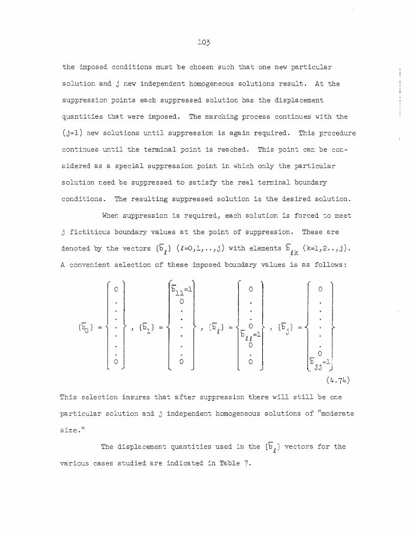
103
the imposed conditions must be chosen such that one new particular
solution and j new independent homogeneous solutions result. At the
suppression points each suppressed solution has the displacement
~uantities that were imposed. The marching process continues with the
(j+l) new solutions until suppression is again re~uired. This procedure
continues until the terminal point is reached. This point can be con-
sidered as a special suppression point in which only the particular
solution need be suppressed to satisfy the real terminal boundary
conditions. The resulting suppressed solution is the desired solution.
When suppression is required, each solution is forced to meet
j fictitious boundary values at the point of suppression. These are
denoted by the vectors (b£} (£=O,l, .. ,j) with elements b£k (k=l,2 .. ,j).
A convenient selection of these imposed boundary values is as follows:
o o
o J
(b. } J
o
This selection insures that after suppression there will still be one
particular solution and j independent homogeneous solutions of "moderate
size. 71
The displacement quantities used in the (b£} vectors for the
various cases studied are indicated in Table 7.
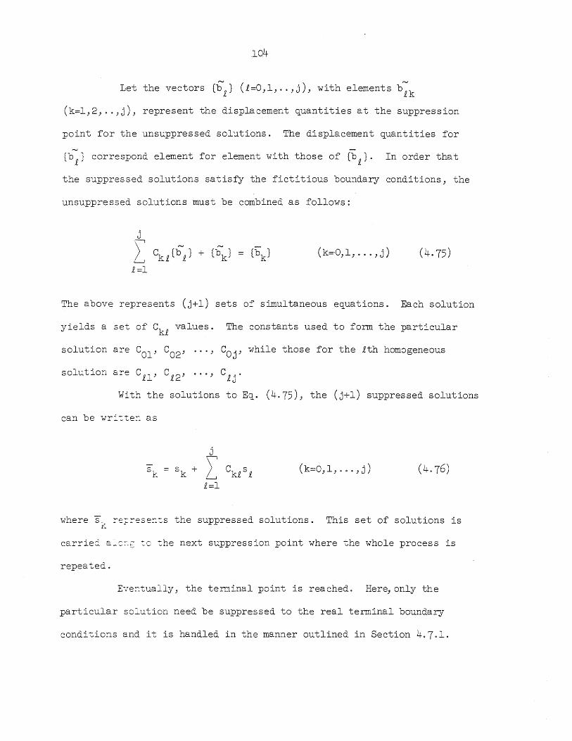
104
Let the vectors (b£} (£=O,l, .. ,j), with elements b£k
(k=1,2, .. ,j), represent the displacement ~uantities at the suppression
point for the unsuppressed solutions. The displacement quantities for
(b£} correspond element for element with those of (b£}o In order that
the suppressed solutions satisfy the fictitious boundary conditions, the
unsuppressed solutions must be combined as follows:
j
I Ck 1 (b 1) + rbk )
£=1
The above represents (j+l) sets of simultaneous e~uations. Each solution
yields a set of Ck£ values. The constants used to form the particular
solution are COl' CO2 ' ... , COj ' while those for the ith homogeneous
solution are Cil' C£2' ... , C£jO
With the solutions to E~. (4.75), the (j+l) suppressed solutions
can be writter. as
S . .K
j
sk + I Ck1 S 1 £=1
(4.76)
where s" ~e;~eser.~s the suppressed solutions. This set of solutions is r.
carrie::: s:C::-.€:" :c the next suppression point where the whole process is
repeated.
Ever.tually, the terminal point is reached. Here, only the
particular solution need be suppressed to the real terminal boundary
conditions and it is handled in the manner outlined in Section 4.7.1.
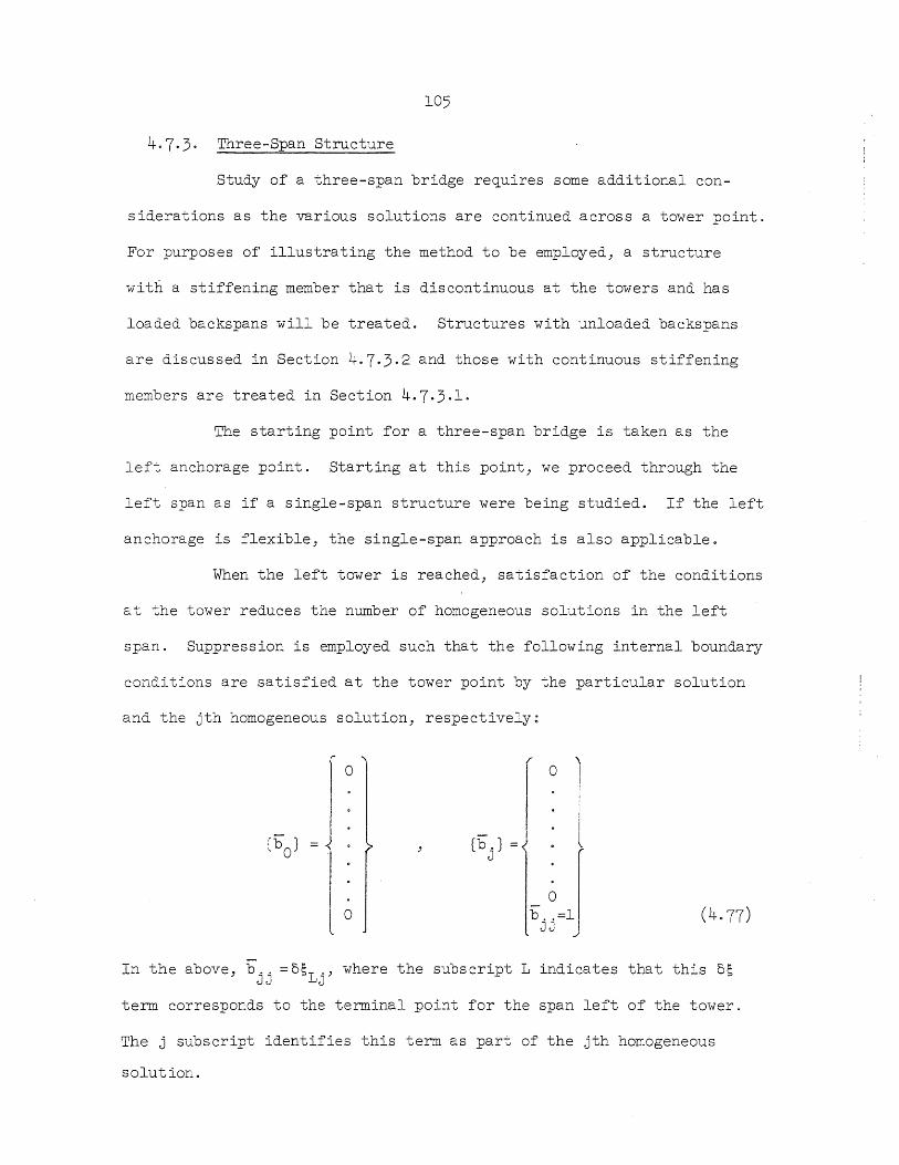
105
4.7.3. Three-Span Structure
Study of a three-span bridge re~uires some additional con-
siderations as the various solutions are continued across a tower point.
For purposes of illustrating the method to be employed) a structure
with a stiffening member that is discontinuous at the towers and has
loaded backspans will be treated. Structures with unloaded backspans
are discussed in Section 4.7.3.2 and those with continuous stiffening
members are treated in Section 4.7.3.1.
The starting point for a three-span bridge is taken as the
left anchorage point. Starting at this point) we proceed through the
left span as if a single-span structure were being studied. If the left
anchorage is flexible) the single-span approach is also applicable.
When the left tower is reached) satisfaction of the conditions
at the tower reduces the number of homogeneous solutions in the left
span. Suppression is employed such that the following internal boundary
conditions are satisfied at the tower point by the particular solution
and the jth homogeneous solution, respectively~
o
(5". ) J
o
In the above) b jj =5~Lj) where the subscript L indicates that this 5~
term corresponds to the terminal point for the span left of the towero
The j subscript identifies this term as part of the jth homogeneous
solution.
106
Thus, upon reaching the tower, we retain two solutions in the
left span, a particular solution and a homogeneous solution having a
unit horizontal displacement at the left tower. These solutions are
determined by Eqs. (4.75) and (4.76) for k = O,j. The homogeneous
solution retained corresponds to the displacement quantity at the tower
that must be continuous with the next span.
At the tower, consider the current point of linearization. Let
6H represent the amount by which horizontal equilibrium is not satisfied
at this linearization point. Referring to Figure 15, we obtain
(H -H ) - (lL -H ) -IC~ = 6H R d -"L d -or T
where ~ and BL are the total horizontal components of cable force right
and left of the tower, respectively. These are computed from Eq. (4.15)
with the displacements of the current point of linearization. The term
ST is the horizontal displacement of the tower point corresponding to
the current point of linearization.
We seek the correct solution, for which 6H vanishes. Letting
(5~-5~) = 6[5HJ, we can write the following for the next linearization:
Here 5~ and 5r~ are the linear variations in ~ and HL, respectively,
for this linearization and 5ST is the corresponding variation in the
horizontal displacement of the tower point. The term 6[5H] represents
the jump in the variation of horizontal component of cable force that
must occur at the tower point. For convenience, this jump is taken in
two parts, one part for each term of Eq. (4.79). For the particular
107
solution
,6.[5H] 0 -M (4080)
and for the homogeneous solutions
(£=1, ... ,j) (4.81)
At the initial point of the center span, a particular solution
and j homogeneous solutions must be initiated. The initial-value
assumptions re~uired for these solutions involve the same displacement
~uantities as are needed for the corresponding single-span case with a
flexible support. These displacement ~uantities are given in Tables 2
through 6, except that the subscript 1 in the tables is replaced ,by R,
which indicates that these quantities correspond to the initial point for
the span to the right of the tower. For the particular solution, the
initial values can be taken to be equal to the terminal values of the
particular solution of the left span, with the exception of 5~! 0 The
procedure for 5~! is described belowo Each of the homogeneous solutions
must evolve from a continuation in 5~ of the homogeneous solution
retained in the left span. Thus, 5~T£ = b~L£ = 5~R£ = 1 ( .e: =1, 0 0 , j ) .
Alse) (j-l) of the homogeneous solutions will contain a unit jQmp in
one of the initial-value quantities from the corresponding terminal
value of the homogeneous solution for the left span. This procedure
ensures that the newly initiated homogeneous solutions are independentu
For the particular solution, E~. (4.80) can be written in
the form
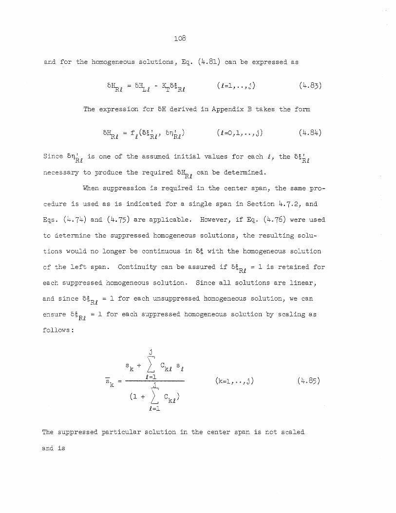
108
and for the homogeneous solutions, Eq. (4.81) can be expressed as
(£=1, .. , j)
The expression for oH derived in Appendix B takes the form
(£=0,1, .. ,j) (4.84)
Since o~R£ is one of the assumed initial values for each £, the o~R£
necessary to produce the required 0RR£ can be determined.
When suppression is required in the center span, the same pro-
cedure is used as is indicated for a single span in Section 4.7.2, and
Eqs. (4.74) and (4.75) are applicable. However, if Eq. (4.76) were used
to determine the suppressed homogeneous solutions, the resulting solu-
tions would no longer be continuous in o~ with the homogeneous solution
of the left span. Continuity can be assured if O~R£ = 1 is retained for
each suppressed homogeneous solution. Since all solutions are linear,
and since o~R£ = 1 for each unsuppressed homogeneous solution, we can
ensure 5sR£ = 1 for each suppressed homogeneous solution by scaling as
follows:
j
sk + I ck£ s£
£=1 (k=l, .. , j) (4.85) sk ~
(1 + L Ck £ )
£=1
The suppressed particular solution in the center span is not scaled
and is
109
(4.86)
Of course, scaling will mean that the homogeneous solutions
will no longer have ~uantities at the suppression point correspondong to
(b£} of E~. (4.74). This is unimportant, however, since these vectors
were ~rbitrarily chosen. No numerical difficulty was encountered as a
result of this scaling.
Since each unsuppressed homogeneous solution in the span
currently being treated is continuous in Os with the homogeneous solution
of the left span, the particular solution in the left span becomes
s = s + o 0"
The resulting particular solutions in left and center spans; respectively,
are continuous in os.
The marching process continues in the center span, suppressing
when necessary. Eventually the right tower is reached. At this point,
we suppress again as re~uired by E~. (4.77). The suppressed particular
solutions in the previous spans are determined as before. Now, only
one homogeneous solution is retained in the center span, and since it
must maintain OST = 1 at the right tower there is a discontinuity in Os
at the left tower with the left span homogeneous solution. To restore
continuity in Os for the homogeneous solution, the homogeneous solution
in the left span is multiplied by the factor
,"0,
110
(1 + t £=1
There are now one particular solution and one homogeneous
solution for the left and center spans, and each is continuous in Os at
the left tower. The solution is continued over the right tower into the
right span in precisely the same fashion as at the left tower.
When the terminal anchorage point is reached, only the par-
ticular solution needb e suppressed which results in the desired
solution to the problem. The terminal boundary conditions for the
various cases and support conditions are the same as those given in
Tables 2 through 6 for a single span.
4.7.3.1. Continuous Stiffening Member
For a discontinuous stiffening member, the only displacement
quantity that is continuous at the tower points is os, the horizontal
cable displacement. In situations where continuous stiffening members
are used, this is no longer the case. Here, or! and or!! are also con-
tinuous at the towers, since both slope and moment of the stiffening
member are continuous functions at the towers.
The technique used for the continuous member does not differ
greatly from that for the discontinuous member. The main difference is
that it is necessary to retain additional homogeneous solutions in the
left span as the solution advances beyond the left tower. One of these
homogeneous solutions in the left span must be split into several in-
dependent homogeneous solutions in the center span. The exact number
will depend on the order of the system. These solutions must be selected
111
so that continuity between the two spans in all the desired displace
ment quantities is ensured and that the boundary conditions at the tower
are not violated. When suppression occurs in the center span) those
homogeneous solutions that are generated from a single le~t-span
solution must be scaled in order to provide proper continuity of the
suppressed solutions. This scaling procedure is identical with that
explained in Section 4.7.3 for the discontinuous member.
When the right tower is reached) a similar technique is used.
The homogeneous solutions that are retained in the center span carry
into the left span and satisfY the continuity and boundary conditions
at the left tower.
4.7.3.2. Unloaded Backspans
For unloaded backspans) there is no connection between the
cable and the stiffening member. Either discontinuous or continuous
stiffening members can be used for this arrangement.
If the stiffening member is discontinuous at the towers, the
side-span decks are merely simply-supported beams and do not flli~ction as
a part of the suspension bridge system. Thus, as the marching solution
advances in the left span, the cable equations are applicable without
external loads. The equations for the center span are determined in
accordance with the suspension bridge case that is applicable.
Regardless of which suspension bridge case is being studied,
the only displacement quantity that is continuous at the tower is Os.
Thus) just a single homogeneous solution is retained in the left span
as the solution advances beyond the left tower. This is analogous to
112
the technique used in Section 4.7.3 except that the left-span equations
are cable equations instead of suspension··bridge equations.
If the stiffening member is continuous at the towers, the side
spans do form an integral part of the suspended system. Here, as the
marching solution advances in the left span, cable equations and stif
fening member equations must be carried separately, with no connection
between the two sets of equations. The external loads are applied to
the stiffening member, while no external forces are acting on the cable.
In the center span, the appropriate suspension bridge equations are
used for the case under consideration.
When the left tower is reached, the manner in which the
solution is carried forward is similar to that described in Section
4.7.3.1. The only difference is that those homogeneous solutions that
are retained in the left span are split between the cable solution and
the stiffening member solutions .. In Section 4.7 .. 3.1 all left..,span homo
geneous solutions were suspension bridge solutions.
4.8. Newton-Raphson Procedure
The Newton-Raphson procedure as applied in the continuous
study is essentially the same as that used in the discrete study. Of
course, in the present instance, a continuous system is being treated.
The application of the Newton-Raphson method in a function space is not
an innovation [for example, see Kantorovich and Akilov (1964)J.
There are a few minor differences in the details of applying
the method here from those employed in the discrete study. There, it
was convenient to shift the reference axis for loads and displacements
113
to the current point of linearizationo Similarly, a new reference con
figuration was established after each load increment. For the continuous
study, such a shift would be more difficult because differentiated terms
would have to be determined in terms of the shifted coordinate system
for each linearization. These terms would be difficult to obtain and
interpret. It is more convenient in this instance to keep all dif
ferentiated quantities in terms of the original dead load coordinate
axes.
It is for this reason that variations were used in the deriva
tion of the linearized equations. The resulting linearized equations
apply at any point in the loading process and all differentiated terms
are with respect to the original dead load coordinat~ system. Actually,
similar variations could~have been used in the discrete study, but such
a procedure is not essential there.
Figure 16 shows schematically how the procedure is applied.
In this figure, the vertical load is plotted as ordinate and some general
displacement quantity d is plotted as abscissa. As in Figures 2 and 11,
the relation between these two variables indicates the increase in
stiffness of the suspension bridge when load is added.
Suppose that the correct displacements have been determined
for some level of load PVb. This loading only represents part of the
total load acting on the structure. Additional load must be applied
above this load level. The next increment of load is PVi and the
figure shows point A as the second point of linearization within this
load increment.
114
For this linearization about point A, all quantities used in
the equations must be the total accumulated values for displacements
corresponding to this point of linearization. The load for this
linearization is 5PV and the displacement quantities 5d, establish a
new set of accumulated displacement quantities for point B on the curve.
The figure shows only the vertical component of load. The
horizontal load components are treated similarly.
The total loads, qvand qH' taken by the cable for this new
set of displacements can be determined from Eqs. (4.8), where H and HI
are found from Eqs. (4.15) and (4.18), respectively. The total loads on
the suspension bridge system corresponding to this set of displacements
are found in accordance with the equations indicated in Table 8.
In each of these cases, Pv and PH represent the total live load
components above the dead load configuration.
Designating P~i and P~i as the load level above PVo and PHo
for the accumulated displacements of point B, we have
(4.88)
I I
When PVi and PHi agree to the desired degree of accuracy with PVi and
PHi' the procedure can be stopped and the latest accumulated displace-
ments are the correct ones for the new incremented level of load
(pvo + PVi on Figure 16). If the total load is on the structure) these
are the final desired results; if not, another increment is added until
the full load is on the structure.
115
4.9. Additional Comments About Continuous Formulation
In the general development of the continuous formulation,
several simplifYing assumptions were made that could quite easily be
relaxed. These points will be briefly discussed in this section.
4.9.1. Nonconstant EI
If EI were not constant, Eq. (4.20) would have the form
(4.89)
Since EI may not be a differentiable quantity, further expansion of the
left side of the above equation may not be convenient. This difficulty
is easily overcome by selecting the continuous function (EIY U) as one
of the uny~own displacement quantities. Once this quantity is
dete~i~ed, yll can be found at each point by dividing by the appropriate
EI. Th:"s can result in discontinuous -rll.
The order of the system is not changed since the highest-order
deri·.~2.-::"·:es (EIt")1l and rli replace the yIV of the case with constant Elo
~. ~" . ..:.. l~o:;,constant k s
~~e quantity k was assumed to be constant in the development s
0: -::-~'::' '::":-:::::s:-~enko beam cases. If k is not constant additional cons
s ije:'::::. -: :"c:-.s are necessary.
I: ks is differentiable, Eqo (4.25) takes the form
5' k1V + k VI S S
Since M! = V, Eq. (4.46) contains an additional term on the right-hand
side equal to 5Mj/ks (1+Si). The solution then continues as before.
If k changes discontinuously, then at each point of diss
continuity, 5 f has a delta-function discontinuity. Looking at E~. (4.24)
we see that since M is continuous y" must also have the same type of
singularity at each discontinuity in k. This re~uires an abrupt jump s
in yf, which corresponds to a concentrated load. These concentrated
loads would be provided by appropriate changes in the hanger loads.
4.9.3. Concentrated Loads and Abrupt Changes in Distributed Loads
In the study presented, only distributed loads were used.
Concentrated loads could also be included without any great difficulty
by treating them as delta-functions.
Integration across these singularities leads'toabrllpt changes
in some of the next-to-highest derivative terms. Just which terms are
affected will depend on the case being studied.
In those cases studied for which partial distributed loads
were involved, no attempt was made to terminate the load at precisely
the correct point. Instead, the beam was divided for computational
purpose, and the load term was included for all points that fell within
the loading ranges and excluded for points outside this range. In this
way, the exact value of the load on the structure is uncertain and the
resulting accuracy is somewhat dependent on how finely the structure is
divided. A more accurate procedure would have been to introduce a
discontinuity in the loading function at precisely the point of change.
Two sets of values would then be carried at each point where the loading
changes--one set corresponding to the left of the discontinuity and the
pther set for the right.

5. NUMERICAL PROBLEMS: RESULTS AND EVALUATION
Several numerical problems are presented in this chapter to
illustrate the use of the two methods of analysis. These problems are
given chiefly as examples of how the methods are applied and to provide
a means for comparison between the two approaches. No systematic
parameter study is attempted; however, some of the results do indicate
trends.
Actual suspension bridges are used as a guide in designing the
sample problems. In some cases, an existing bridge is used in its
entirety, while in other cases modifications are made. The problems
treated are, therefore, realistic with regard to dimensions and physical
properties.
5.1. Single-Span Unstiffened Suspension Bridge
The unstiffened suspension bridge is simply a cable that is
initially held in the shape of a parabola by the assumed horizontally
distributed dead load. Case A of the continuous formulation is valid
for this arrangement.
The prime reason for studying the unstiffened bridge is to
gain understanding of the cable equations. This is an important area
since the cable behavior is the cause of the nonlinear response of a
suspension bridge. Thus, by studying the unstiffened bridge without the
interference of the deck response, greater insight is gained in the
functiorling of the techniques used for solving the nonline.ar equations.
117
i18
The structure treated in Sections 5.1.1 through 5.1.4 has the
same dimensions and properties as the center span of the original,
unstiffened George Washington Bridge. The analyses made of this single-
span structure do not, of course, apply to the response of the center
span of the actual bridge, for here the cable support points are assumed
to be fixed,* whereas in the three-span structure these points are
flexibly restrained.
The important physical characteristics of this structure are
given in Figure 17 under Problems 1.1, 1.2, and 1.3.
5.1.1. Unsymmetrical Loading Condition (Problem 1.1)
For unsymmetrical loading, large displacements occur and the
nonlinear response of the structure can be significant. Thus, it is
useful to use an unsymmetric loading condition as a means for comparing
the res~lts as computed by the two methods of analysis. This compari-
son sho~lj indicate whether the two methods predict the same nonlinear
response c: ~he structure.
f.. :ive load of 7.2 kips/ft of bridge is distributed over a
lengt:-: ~.~ :. ~i = 1050 ft adjaceritto the le.ftto'Werofthe structure.·
describ~i i:-. S~ction 5.1 and Figure 17. In the discrete method, 20 links
are usei ~:-. ::-:~ chain system, while 100 divisions are used in the con-
t · . . H1UOUS ::'.e::-.::::::'. The resulting displacement quantities at the tenth
points are giYen in Table 9, where good agreement is indicated. For
each case) the load is applied in two increments.
* In the discrete method, a stiffness of tH = tv = 1. x 1010
kips/ft is used. This produces displacements at the tower points that are zero to the number of decimal places carried.
The displacements are plotted in Figure 18. Since the results
of the two methods agree so closely, only one curve appears in each
plot. The discrete results would actually be composed of straight lines
inscribed within the continuous curve with vertices at the tenth points.
In Figure 19, the load-displacement relationships are shown for the
horizontal and vertical displacements at the two-tenths point. The non
linear response can be seen in these diagrams. The departure from the
linearized theory increases rapidly with further increase in live load.
For this structure, the dead load is quite large. This tends to stiffen
the structure and thereby limits the magnitude of the displacements and
the nonlinear response.
5.1.2. Temperature Change (Problem 1.2)
As was indicated in the development of the discrete method,
temperature change has the effect of some equivalent load. In the con
tinuous formulation, equivalent temperature loads do not enter ex
plicitly, but the end result of temperature change should be the same.
The structure described in Section 5.1 and Figure 17 is used.
A live load of 7.2 kips! ft of bridge is applied to the entire structure
and a temperature change of +550 F is specified. As in Problem 1.1, a
chain of 20 links is used in the discrete study and 100 segments are
used in the continuous study.
The tabulated and plotted results are given by Table 10 and
Figure 20, respectively. Agreement between the two methods is very good.
The true polygonal plot of the discrete method has not been drawn, but
it would be inscribed within the continuous curve. The case of no
temperature change is also indicated in Figure 20 for comparison.
120
The details of applying the two methods differ considerably
in this instance. In the discrete method, the equivalent loads are
applied as the first increment of load, followed by two increments of
live load. In the continuous method, the temperature effect is not
explicitly expressed as equivalent load. Here, two increments of live
load are applied, the full temperature change being included for both
increments.
The two methods use different paths of loading, as can be seen
in Figure 21. The solid line represents the relationship between the
intensity of live load and the displacement at mid-span. The negative
o values indicate that for a temperature change of +55 F, negative live
load would have to be applied if the displacement is to be less than
2.619 ft. This value is the mid-span displacement caused by temperature
acting alone.
In the discrete method, the origin for loading is taken at a
negative load level (point A, Figure 21). The first increment of load
corresponds to 6.6 kips!ft at mid-span and produces a displacement of
2.619 ft. The first increment of the actual live load is applied from
point B.
In the continuous method, the temperature effect is not treated
directly as equivalent load. Here, the first linearization occurs at
point C of Figure 21 and a load of 3.6 kips!ft produces the displace-
ments shown. Although temperature change is not reflected in a load
term in this method, it is reflected in establishing the slope for the
first linearization. This slope is identical with that of the first
linearization of the discrete analysis. However, even though an
121
equivalent temperature load is not employed in the first linearization,
the loading path returns to the real load-displacement plot when the
load corresponding to the displacement of the first linearization is
determined. This is indicated as point D in Figure 21. The second
linearization of the first increment of live load takes place at this
point with a load of approximately 6.66 kips/ft.
Even though the loading paths are quite different, the final
results agree very well. The continuous method could have been formu-
lated to include equivalent temperature loads. This would have been
the result of considering temperature variation terms explicitly in the
linearized equations. The disadvantage of not treating temperature
variation separately is that the effects of temperature acting alone
cannot be determined.
Variation in Number of Links in Chain System of Discrete Analysis (Problem 1.3)
It is of interest to know how the selection of the number of
links for the chain system affects the final results. If possible, a
node should be placed at each hanger point. However, for very long
spans, this procedure leads to the solution of large numbers of simul-
taneous equations. It would be convenient, therefore, to use fewer
nodes than the actual number. Such a reduction was employed in
Problems 1.1 and 1.2.
Consider again the structure described in Section 5.1 with a
uniformly distributed load of 7.2 kips/ft of bridge along the entire
span. This structure is analyzed three separate times, the number of
links being 10, 20 and 40. The vertical displacement at mid-span and
122
the horizontal displacement at the two-tenths point are plotted against
1/N2 in Figure 22, where N is the number of links. llie resulting plot
is a straight line in each case. The vertical scale is greatly
exaggerated in this figure. Actually, the agreement for all three
values of N is ~uite good. Thus, it seems apparent that for very long
structures with many node pOints, satisfactory results can be determined
* by using a model of condiderably fewer elements.
Upon extrapolating each line to 1/N2 0, values for an
infinite number of elements is obtained. lliis would represent a con-
tinuous system. The values obtained are 2.8717 ft and -0.24516 ft for
the vertical and horizontal displacement, respectively. These compare
very well with corresponding values of 2.87172 ft and -0.245168 ft,
which were determined by the continuous method of analysis using 200
segments.
Variation in the number of segments for the continuous method
does not admit of a similar interpretation. In this case, the same
differential e~uation is being solved at each point regardless of the
number of points used. Thus, the same continuous structure is being
approximated regardless of the space interval. Differences that do
occur come from truncation and rounding errors in the solution, which
will depend on the space interval chosen. In the discrete case, however,
a change in the number of elements actually changes the structure. As
long as the space interval for the continuous case is such that the
number of cycles per step of integration does not exceed 5 to 8, it has
been found that the results are satisfactory.
* In the stiffened suspension bridge, this conclusion is not always valid. (See Section 5.2.3)
5.1.4. Effect of Loading Path
For both methods of analysis) problems were studied in which
different paths were used in building up to the total live load on the
structure. It was found that for all cases studied) the values obtained
indicated no sensitivity to the loading sequence. This suggests the
presence of a unique solution. However) formal proof of this from the
nonlinear equations is not available.
5.2. Hanger Elongations
Hanger elongations have no effect in the case of an unstif
fened bridge. This is true because there is no change in the load
carried by the cable as a result of these elongations. However) in the
case of a stiffened bridge) hanger elongations do have an effect. In
this case the hanger elongations allow the deck to move through addi
tional deflections which alter the hanger loadso It is the object of
this section to study the changes caused by these elongations 0
Most treatments of the classical deflection theory have
ignored hanger elongations. Those that do mention the subject indicate
that the effect is negligible 0 Some recent studies have included hanger
elongations) but no attempt has been made to study the effect of their
inclusion.
The structure used for this phase of the study is a single
span stiffened bridge. The dimensions and physical properties for this
span are selected from the center span of the Manhattan Bridge. This
structure has a fairly stiff deck. If there are any significant changes
as a result of the hanger elongations) they should) therefore, appear in
12~
this case. The structure is described in Figure 17 under Problems 2.1
and 2.2. Both cable and stiffening member supports are assumed to be
fixed.
5.2.1. Bridge Without Elongations (Problem 2.1)
The structure described above is loaded with a live load of
4 kips/ft over the entire spano The displacements and moments are first
determined on the assumption that the hangers are inextensible. Both
the continuous and discrete methods are used for the analysis. In the
continuous study a Bernoulli-Euler beam is used for which Case B is the
correct formulation. In the discrete case the stiffening member is also
taken as a beam. The results are given in Table 11 and are plotted in
Figure 23. The two methods agree very well. Of course, both the cable
and the deck have equal vertical movements and are represented by the
same curve in Figure 23. Ten links are used in the chain system of the
discrete study and 100 divisions for the continuous treatment.
The values for moments agree well at the computed points, the
discrete moment diagram again being inscribed within the continuous
moment diagram. For the actual structure, the moment diagram would be
inscribed within the continuous diagram with shorter straight line
segments, because the real structure would have many more than ten links
in the chain system.
The two methods lead to end reactions that differ considerably.
This is necessarily the case because this reaction is equal to the end
shear, which in turn is equal to the end slope of the moment diagram.
For the actual structure, which has about 60 hangers, the reaction would
fall somewhere between the two values obtained.
125
502.2. Bridge with Elongations (Problem 2.2)
Here) the same structure that was treated in the previous
section is analyzed) except that hanger elongations are now included.
Case D is the correct continuous fonnulation for this problem. Once
again) ten links are used in the discrete study but 200 di.visions are
necessary for convergence in the continuous method. Also) 50 suppres-
sions are required here, whereas only six were needed in the case with-
out elongations.
In the continuous study the hanger area is taken as 0036 in2/fto
The hangers used in the discrete study have cross-sectional area of
53 in2 . The modulus of elasticity for the hangers is taken as 16)000 ksio
The results of the two methods are tabulated in Table 12 and
are also presented in Figure 24. The only significant change from the
case of no elongations is in the end sections of the moment diagram.
The end shear and reactions are) therefore) altered considerably.
The difference between the moments and end reactions found by
the two methods when hanger elongations are included is also significantu
Once again) the results for the actual structure would fall somewhere
between the two extremes 0
50203" Effect of Hanger Elongations
In each case studied above) the two methods give results that
agree quite well in most regionso It is of interest to compute the
changes that occur in moments and displacements when hanger elongations
/
/ are allowed. This is done for each method of analysis and the results
are shown in Figure 25. In developing these curves) iLtermediate
points are plotted in the end sections for the continuous study in
126
addition to those given in Tables 11 and 12. Some accuracy is lost
here because small differences of large ~uantities are taken. Very
small departures from symmetry for the individual cases are then greatly
magnified. However, the two separate approaches do indicate the same
general behavior, and a great deal can be determined in a ~ualitative
way from these results.
Figure 25 shows ~uite clearly that for the loading treated,
the hanger elongations have their greatest effects on ~uantities adjacent
to the supports. This is where the hangers are longest and the elonga
tions are greatest. However, hanger elongations are restrained very
close to the support because of the fixed support points for both the
cable and the deck.
An unloading of the cable is associated with the hanger elonga
tions. This unloading is greatest in the end portions, and leads to an
upward and inward movement of the cable in these regions. Since the
change in cable load is ~uite small, the cable length remains essentially
constant. Thus, the central portion of the cable must displace downward.
The deck must take the load that is no longer taken by the
cable. This leads to an increase in the deck deflections. In the middle
60 percent of the span, the additional deck deflection is almost constant.
The center portion with its short hangers has very small hanger elonga-
t ions. The change in the deck deflection for this region~. is,;;·' therefore,
mostly a result of the increase in vertical cable displacement. As the
cable displacements decrease from mid-span toward the support, the
increase in hanger elongations causes the resulting change in deck de
flection to remain almost constant in a large portion of the span.
127
Since the curve of changes in deck deflection is very flat
for the central 60 percent of the structure, there is very little
change in curvature and moment. However, in the end regions, the
changes in curvature and moment are quite pronounced 0
For all of the quantities plotted in Figure 25, the two methods
of analysis indicate the same general behavior. Quantitatively, the
two methods yield results for the central 80 percent of the structure
that agree very well. For this region, the changes caused by hanger
elongations are quite small indeedo However, near the ends of the span,
the two methods differ considerably for the structure studied. It is
this region which contains some changes of considerable magnitude.
The differences in results for the two methods in the exterior
por~io~s would be much less if the actual number of hangers were used
i~ the discrete study. In fact, this study suggests that the only area
of s~~.ificant disagreement between the two methods would be from the
SUPPOY: :0 the first hanger point. In this region, the continuous
always lead to reactions and moments that are greater than
wct:.l:::' C<~:'''':':- ir: the real structure. However; in the discrete method~
2.:-".y 8. ::e::-.p: :0 study a structure with fewer hangers than the actual
~ead to reactions and moments that are too small in this
I: is of interest to note that the value of H is essentially
uncha~gei by hanger elongations. This agrees with the findings of
Johnson, Bryan and Turneaure (1911). However, their conclusion from
this fact that the effects of hanger elongations are small is not borne
out by this investigation. It is true that the average effects are
128
small; nevertheless) local changes of considerable significance may be
present.
From a mathematical point of view) the results are the con
sequence of the introduction of an edge effect associated with the
raising of the order of the system of differential equations by con
sidering a large) but finite, hanger stiffness. Both the local character
of the large effects and the great increase in the number of suppressions
required point to this interpretation.
These conclusions about the effect of hanger elongations cast
some doubt on the adequacy of any continuous theory of suspension bridges
for the prediction of end shears in the stiffening member.
5.3. Shearing Deformation
Another topic of interest is the effect of shearing deforma
tion on the response of a suspension bridge. Timoshenko (1943) touches
on this subject briefly with regard to the conventional deflection
theory.
The structure used in this study is the same as that used in
the hanger elongation study of Section 5.2. The dimensions and physical
properties of this structure are given in Figure 17 under Problems 3.1
and 3.2. Again) both hanger and support points are assumed to be fixed.
5.3.1. Bernoulli~Euler Beam as Stiffening Member (Problem 3.1)
The bridge is loaded with a live load of 4.0 kips/ft over the
left one-third of the spano The displacements) shears and moments are
determined on the assumption that the stiffening member is a Bernoulli
Euler beam in which shearing deformations are ignored. In the discrete
129
method, a beam with the stiffness indicated in Figure 17 is used as the
stiffening member. For the continuous study, Case B is the appropriate
formulation. The results of the discrete and continuous analyses are
given in Table 13 and Figure 26. Since hanger elongations are ignored,
the vertical displacement values are for both the cable and stiffening
member.
Ten links are used in the chain system of the discrete method,
whereas the structure is divided into 100 divisions for the continuous
study. The plot of shears in Figure 26 demonstrates again the dif-
ference in end shear between the two methods. Of course, as more hangers
are used in the discrete study, this difference would decrease.
In general, the two methods give results that show very good
agreement. The shear diagrams are necessarily of different shape
because of the difference in the assumed hanger arrangement for the two
methods. However, the average values of the continuous shears within
each panel agree well with the discrete values.
503.2. Timoshenko Beam or Truss as Stiffening Member (Problem 3u2)
The same problem that is described in the previous section is
examined again in this section. How,ever, in this instance a stiffening
member that includes the effect of shearing deformations is used. For
the continuous method, the Timoshenko beam is used, so that Case C is
applicable. The discrete study would take a truss as the stiffening
member and the stiffness matrix for the truss would include the effect
of shearing deformations. The TLmoshenko beam constant, as derived from
E~. (4.27), for the assumed stiffening truss is 0018 x 10-5 kips-l. As
130
in the previous section, hanger elongations are ignored and, therefore,
vertical displacements of the cable and truss are equal.
The results of the continuous study are given in Table 14.
The discrete results are not reported here because in treating the full
stiffening -truss of this problem the capacity of STRESS was exceeded.
This limitation is a temporary problem peculiar to the current version
of STRESS and will constitute no restriction in future versions. For
the vertical scale that is used, the plotted results would be essentially
the same as for Problem 3.1 and, therefore, these results are not
plotted separately.
5.3.3. Effect of Shearing Deformations
The effect of shearing deformation is to reduce the stiffness
of the sti~fening member. This reduction in stiffness requires that
more load be carried by the cable. This redistribution is obvious from
the char.ges that occur in the cable displacements when shearing deforma
tions are allowed (see Figure 27). The load transferred to the cable has
essentia::y tte same distribution as the live load carried by the cable
for the :::ase ~ .. ;ithout shear deformations. This fact is apparent since
the shapes c~ the diagrams of displacement changes (Figure 27) have the
same ge~eya_ s~apes as the displacement plots of Figure 26.
Si~ce the cable carries more load, the stiffening member must
carry less load. This is indicated by the decrease in both shear and
moment that occurs when shearing deformations are permitted. Again, it
is clear from Figures "27 and 26 that the redistribution of load as a
result of shearing deformations is essentially proportional to the
131
loading on the Bernoulli-Euler beam studied in Section 503010 The
changes in shear and moment are of opposite sign to the Bernoulli
Euler values. This reflects the unloading of the stiffening membero
For this problem) shearing deformations reduce the shear by
about 2 percent and the moments by about 105 percent. However) it must
be remembered that the change diagrams come from taking differences of
large quantities of approximately the same magnitudeo For this reason)
Figure 27 is not very reliable from a quantitative point of view.
However) in terms of qualitative behavior) this study indicates clearly
the order of magnitude of the effect p
One problem was studied in which both hanger elongations and
shearing deformations were included 0 This problem was solved by Case E
of the continuous formulation. The detailed results are not reported
here; however) it should be mentioned that the computational problems
were essentially the same as for the case where just hanger elongations
were included. The inclusion of shearing deformations created no inter
action that created any additional computational difficulties.
5040 Sample Problems for Three-Span Bridges
In this section) a few sample problems are presented for a
full three-span structure 0 The structure selected for all the problems
of this section is the Manhattan Bridgeo This structure is described
in detail in Figure 17 under Problems 401) 4.2 and 4.3. In the discrete
method) the stiffening member is taken as a beam in each span with the
stiffness indicated in Figure 170 Case B is the appropriate formulation
for the continuous methodo
132
It is assumed that the tower saddles are mounted on rollers
and that the anchorage points are fixed. This will yield results for
which H is constant throughout all spans) which corresponds to the
assumption generally made in the conventional deflection theory. This
is done in order to make some comparisons with the work of previous
investigators. In Section 5.4.2) one problem is worked in which the
tower stiffness is included in order to demonstrate its effect.
For the discrete method) the left and right span cables are
each divided into five links and the center span cable has ten links.
Fifty segments are used for each side span of the continuous study while
the center span is divided into 100 divisions.
5.4.1. Maximum Mid~Span Deflection (Problem 4.1)
The maximum mid-span deflection of the main span is attained
by applying full live load to the center span (with the side spans
unloaded) and maximum positive temperature change.
In this case) the live load intensity is 4.0 kips/ft and a
temperature change of +55°F is prescribed. The problem is solved by
both the discrete and continuous methods and the resulting displace
ments are given in Table 15 and Figure 28. The displacement diagrams
for the discrete method would actually be composed of a series of
straight lines between the node points. The vertical displacement
values apply to both the cable and stiffening member) since hanger elonga
tions are neglected. Agreement between the two methods is generally quite
good. All differences are w'ithin 2 to 3 percent of the maximum values.
The maximum vertical displacement is 10.697 ft and 10.835 ft
by the discrete and continuous methods) respectively. These values
133
differ by only a little over 1 percent. Presumably, this difference
would decrease as additional hanger points were considered for the dis
crete method. Johnson, Bryan and Turneaure (1911) obtain a value of
11.677 ft for this quantity. This value should be compared with
10.835 ft of the continuous study since both refer to continuous
formulations.
It should not be expected that the results of previous investi
gators agree precisely with those presented here because the formulations
of the conventional deflection theory and the continuous theory developed
here differ considerably.
504.2. MaximurrL Mid-Span Moment '{Problem. ,4~ 2)
For maximum mid-span moment in the center span) the full live
load of 4.0 kips/ft is applied from k 8 to k = 12 (see Figure 17).
There is no other load on the structure and a change in temperature of
+550 F is used. This loading agrees with that which is suggested by
Johnson, Bryan and Turneaure (1911) for this condition.
Once again, the problem is worked by both methods cf analysis.
The resulting displacements and moments are indicated in Table 16 and
Figure 29. The vertical displacement values are for both the cable and
stiffening member. The straight line segments of the diagrams for the
discrete method are not included in the plots. Agreement between the
two methods for vertical displacements and moments is quite good;
however, the horizontal displacements do not appear to compare as well.
Here, the displacements are very small in some regions and it is mis
leading to compare the two methods directly at each point. If the
134
differences are compared to the maximum values present, it is seen that
they are ~uite small.
Some of the differences in these solutions are believed to be
related to the problem of partial loading that was discussed in Sec
tion 4.9. The method used for partial loading in the continuous method
does not produce the exact distribution of load that is desired. The
fact that H for the continuous study is appreciably smaller than that of
the discrete study further suggests that the loadings are not exactly
the same in the two methods.
The maximum moment is 86,057 f~kips and 85,911 ft-kips by
the discrete and continuous methods, respectively. These compare fairly
well with 89,710 ft-kips of Johnson, Bryan and Turneaure (1911).
The above results are for a case in which the saddles are
mounted on rollers. When the saddle is assumed to be fixed to the tower
and a tower stiffness of KT = 200 kips/ft is used, there are some minor
changes. Since this problem was solved by the continuous method, the
following comparisons are made with the continuous solution of
Problem 4.2.
The introduction of tower stiffness reduces the horizontal
cable displacement at the tower by about 2 percent. This restraining
effect decreases the positive moment at mid-span by about 2 percent and
decreases the maximum side span negative moments by about 2.5 percent.
These changes are accompanied by an increase in H of about 1.2 percent
in the center span and a decrease in H of 0.7 percent in the side spans.
135
504030 Load Traversing Technique (Problem 403)
As waSt explained in Sections 308 and 408) the Newton-Raphson
method requires an incremental application of the full live loado The
essential feature is that an increment of load is placed on the struc
ture at some known equilibrium configuration) and the new configuration
is sought 0 In all discussions up to this point) it has been assQ~ed
that the increments were distributed proportionately to the live loado
Tnat is) for some given distribution of live load) the total live load
is attained by incrementing the full distribution proportionately until
the total prescribed load acts on the structure 0 However) increments of
load need not be of this type; they can involve changes of spatial dis
tribution as wello Als~ load increments need not be positive; an
increment of negative load will decrease the load on the structure 0
A useful application of load incrementing in whi,ch the spatial
distribution is changed is presented in this sectiono In this case) a
train is followed across the bridge 0 Each load increment i,nvolves
adding some specified length of'load ahead of the previously loaded
section and simultaneously removing an equal length of load from the
rear of the previously loaded sectiono Thi.s load increment represents
the changes in load that occurs as the train advances by the prescribed
distanceo
The same bridge that was used in the previous two sample
problems is used here 0 This is described in detail in Figure 170 A
load of 2067 kips/ft over a length of 480 ft is used to represent the
train loadingo This is the loading for each cable and assumes two trains
per cable traversing the span in parallel 0 The load is based. cn the
passenger car built by The Budd Co. in 1964 for the New York Transit
Authority (BMT Division). Each car weighs 40 tons and is 60 ft long
(1.33 kips/ft). * An eight-car train is assumed (480 ft).
In addition to the initial position of the train at the extreme
left of the structure, nine other load positions are considered. There-
fore) each increment of load corresponds to an increase in load for
271 ft ahead of the previous train position and a cancellation of load
for 271 ft from the rear of the train at its previous position.
The ten positions of load are indicated in Figure 30. Loadings
1 through 5 are shown ~or the indicated train positions as the train
traverses the structure from left to right. All quantities of interest
for loadings 6 through 10 are available from the first five loadings
by taking a mirror image as indicated in Figure 30. The inclined dotted
lines indicate the train movement and the positions at which an analysis
is made.
This problem is solved only by the continuous method (Case B).
Adequate evidence has been gathered to show that the discrete and con-
tinuous methods yield results that are in good agreement. The same
procedure could quite easily be used with the discrete method.
At each loading position that is considered as the train
traverses the structure) the displacements, slopes and moments are
plotted in Figures 31 through 34. Figure 32 indicates that corresponding
to each load position, the structure deforms with a pronounced sagging
curvature under the train. This same point is shown in Figure 34 in which
* This information was provided by Professor W. W. Hay of the University of Illinois.
137
a region of high positive moment is always present under the loaded area o
The same is also reflected in Figure 33) which shows that with the
exception of loadings 3 and 8) the train is always progressing up a
slight deflection gradient 0 The exceptions are a result of the train's
being positioned over a tower support point where the deflection
gradients at the ends of the train are approximately zeroo L~e final
results of this kind of load traversing scheme could easily be presented
in the form of envelopes of maximum effectso
Loading 5 represents a train position that is not quite
centered about mid-spano However) we can see that the displacement and
moment patterns are very near to those of Problem 402 (Figure 29) which
considers a similar partial loading centered about mid-spano
This technique is useful since a great deal of information
becomes available from a single computer run 0 This procedure may be
especially significant at present with the increase in the use of rapid
transit trains in large metropolitan areas 0 Several recent studies for
rapid-transit systems have considered using existing suspension bridges
to carry rail traffic 0
6. CONCLUSIONS AND RECOMMENDATIONS FOR FURTHER STUDY
6.1. General Conclusions
Each of the two methods of analysis presented in this study
provides a sound procedure for suspension bridge analysis. Although
the two methods differ significantly in their mathematical formulation,
they are based on essentially the same general assumptions regarding
the over-all response of the structure 0 The results for a variety of
sample problems show very good agreement between the two methods~
However, each method has certain advantages and disadvantages with
regard to its application.
The discrete method developed in Chapter 3 uses a mathematical
model with the capacity of representing the real structure very closely.
However, such a realistic statement of the problem re~uires the solution
of large numbers of nonlinear simultaneous algebraic e~uations. Use of
the Newton-Raphson procedure (Section 3.8) makes it possible to solve
these equations by considering linearized equations which are solved
repeatedly. The resulting computational effort is considerable. When
the mathematical model has fewer hangers than the real bridge, the number
of equations that must be solved can be reduced. However, this pro
cedure can introduce errors in the end reactions and shears (Section
5.2.1 and 5.2.2).
The continuous method is formulated in Chapter 4 as a nonlinear
boundary-value problem for ordinary differential equations. However) each
cycle of the Newton=Raphson procedure used'inthe:solutiontechnique involves
.138
139
solving a set of linear initial-value problems (Section 4.8). Numerical
difficulties are encountered for which a "suppressionl! technique is
required (Sections 4.7.2 and 4.7.3). Within each linear solution)
several suppressions may be required; however, each suppression requires
the solution of five simultaneous algebraic equations at most. There
fore) this method is considerably faster than the discrete method unless
a very large number of suppressions is required. The departure of the
mathematical model from the real structure can cause considerable
errors in the end shears and reactions of the stiffening member
(Sections 5.2.1 and 5.2.2).
The success of the Newton-Raphson procedure in solving the
ordinary differential equations of the continuous method shows its
promise for solving other nonlinear systems whose behavior can be ex
pressed by systems of ordinary differential equations.
The continuous formulation presented here differs from the
classi2a~ deflection theory in two important ways. First) horizontal
cable d::"s}:lacements are admitted throughout the development) eliminating
the ~.ee:' :0::' an explicit "cable condition" of compatibility. Secondly)
the ~.2:-._::.:-.ea::, terms in the cable equations of equilibrium are fully
ta:r:e:-. ::-.:::: 5.2Count.
Tie continuous formulation demonstrates the power of the sup
pressic~ :ech~ique as a tool in numerical analysis. Early portions of
this st~dy included several abortive schemes for solving the initial
value problems. Each of these approaches eventually failed by resulting
in enormous displacements before a complete sweep could be executed.
Without the suppression scheme) or some equivalent method) this difficulty
could not have been resolved. Even in cases where suppression is
re~uired every few steps, as when hanger elongations are included
(Section 5.2.2), good results were obtained. Such cases may be some
what impractical because the solution time increases considerably and
the large number of operations may make the results less reliable
because of rounding and truncation errors.
Inclusion of hanger elongations creates considerably numerical
difficulty for the continuous method. This problem results from edge
effects that are associated with raising the order of the system of
differential e~uations by considering extensible hangers. The larger
number of suppressions for this case, which was discussed earlier, is a
result of these edge effects. For the discrete study, hanger elonga
tions create no numerical problems except that inverses of large
matrices must be obtained.
Both methods show that the effect of hanger elongations is
to increase sharply the end reactions and shears of the stiffening
member (Section 5.2.3). The continuous method will always yield end
shears in this. case that are considerably greater than the correct
values. As a result, all continuous theories may be inade~uate for pre
dicting end shears and reactions for the stiffening member. The
discrete method will yield the correct end shears only if the actual
number of hangers is used. If fewer than the actual number are"used,
the resulting end shears will be too small.
Shearing deformations will occur in truss-type stiffening
members. The result of these deformations is to reduce the stiffness
of the stiffening member. This produces an internal redistribution of
load from the deck to the cable. This study suggests that this internal
redistribution is roughly proportional to the loading on the stiffening
member obtained when shearing deformations are not considered
(Section 5.3.3).
The load traversing method (Section 5.4.3) is a convenient
application of the Newton-Raphson procedure that can be used to trace
the movement of a train across the structure. This scheme would be
particularly useful in studying the effect of train loadings on existing
bridges.
6.2. Recommendations for Further Study
Many additional applications of the methods presented in this
study are possible. Some topics for further study are discussed in
this section.
In addition to the two methods studied, a third method may be
possible that includes the advantageous features of each of the other
two methods and avoids their respective disadvantages. This third
method would be a discretized formulation of the suspension bridge
problem as a nonlinear boundary-value problem. It would, however,
contain the central features of the continuous study in that it would
be solved as a set of initial-value problems. This technique preserves
the advantage of having to solve just a few simultaneous equations at
each suppression point. This method, however, will also have the
advantage of taking into account the discrete nature of the hangers and,
therefore, will yield the correct results when the full number of
hangers is used. Since large numbers of simultaneous algebraic
142
equations are not involved, there is no disadvantage in employing the
correct number of hangers.
For either of the methods studied here or for the method
proposed above, the cable equations should be generalized to include
transverse displacements. This would make them applicable for studying
other cable systems such as those' employed in roof systems, guyed
structures apd antenna systems.
These more general cable equations could also be used in formu
lating a method of suspension bridge analysis that treats the complete
space structure. In this case, the effect of hanger inclinations should
be included because they can cause transverse loading in the horizontal
planes of the stiffening member system. For the planar system treated
in this study, the hanger inclinations cause only axial loads along the
stiffenir.g member, which are unimportant. In all cases, these inclina
tions produce small horizontal components of force at the cable
connectior. points.
O~ce the full equations for the three-dimensional suspension
bridge are :o~ulated, many problems can be studied. A comprehensive
analysis C: 6. bridge can be made for any loading condition and the
complete respo~se) including torsional effects) can be determined.
Vibratio:-. s,,:·~d.:'es can be made) including vertical, transverse, and
torsiona': exc:':,ations. This general formulation will also provide for
the straigttforward analysis of suspension bridge systems that do not
have their cables in vertical planes. Major bridges of this type have
occasionally been proposed. Small pipeline or foot bridges with this
arrangement are common.

.143
It is only after a complete analysis of the three-dimensional
structure is available that the d~velopment of an automated design
process for suspension bridges can be attempted.
LIST OF REFERENCES
Asplund, S. 0., 1945, liOn the Deflection Theory of Suspension Bridges," Ingenj8rsvetenskapsakademins Handlinger 184, Stockholm.
Asplund, S. 0., 1949, "Deflection Theory Analysis of Suspension Bridges, II Publications, Interna tional Association of Bridge and Structural Engineering.
Asplund, S. 0., 1958, IIColumn - Beams and Suspension Bridges Analyzed by Green! s Matrix, II Chalmers Tekniska Hogskolas Handlinger, Nr. 204.
Asplund, S. 0., 1966, Structural Mechanics: Classical and Matrix Methods, Prentice-Hall, Inc., Englewood Cliffs, N. J., Chapter S.
Bl~ich, F.,et al, 1950, The Mathematical Theory of Vibration in Suspension Bridges, USGPO,Washington, Chapter 8.
Crandall, S. H., 1956, Engineering Analysis, McGraw-Hill Book Company, Inc., New York, p. 160.
Fenves, S. J., 1965a, STRESS, The Structural Engineering System Solver, Users Manual, Department of Civil Engineering, University of Illinois, Urbana, Illinois.
Fenves, S. J., et al, 1965b, STRESS, A Reference Manual, MIT Press, Massachusetts Institute of Technology, Cambridge, Mass.
Godard, T., 1894, "Recherches sur le calcul de la resistance de tabliers des ponts suspendus, " Annales des Ponts et Chaussees, Vol. 8.
Hoff, N. J., 1956, The Analysis of Structures, John Wiley and Sons, Inc., New York, pp. 138-151.
Jakkula, A. A. ,1936, liThe Theory of the Suspension Bridge, II Publications, International Association of Bridge and Structural Engineering.
Johnson, J. B., Bryan, Co Eo, and Turneaure, C. Eo, 1911, The Theory and Practice of Modern Framed Structures, Part 2, John Wiley and Sons, New York.
Kantorovich, L. V., and Akilov, G. P., 1964, Functional Analysis in Normed Spaces,Pergamon Press, The MaCMillan Company, New York, Chapter 18 (translated from the Russian edition of 1959).
Karol, J., 1938, "A ~artial Influence Line Procedure for Suspension Bridge Analysis by the Deflection Theory, II Ph.Do Thesis, University of Illinois, Urbana.
144
Jl45'
Kuntz, C. P., Avery, J .. P., and Durkee, J. L., 1958, "Suspension Bridge Truss Analysis by Electronic Computer,Y1 Conference Papers, Conference on Electronic Computation, American Society of Civil Engineers.
Langhaar, H. 10, 1962, Energy Methods in Applied Mechanics; John Wiley and Sons, Inco, New York, po 42-430
Livesley, ~. Ko, 1964, Matrix Methods of Structural Analysis, Pergamon Press, The MaCMillan Company, New York, po 241-247.
Melan, J., 1888, "Theorie der eisernen Bogenbrucken und der " Ii Ii Hangebrucken, Handbuch der Ingenieurwissenschaften, 2nd Edition,
1888, Leipzig.
Newmark, No Mo, 1943, "Numerical Procedure for Computing Deflections, Moments, and Buckling Loads J Ii Transactions of the American Society of Civil Engineers, Vol 0 108, New Yorko
Newmark, No M., 1959, vrrA Method of Computation for Structural Dynamics,ii Journal of the Engineering Mechanics Division, Proceedings of the American Society of Civil Engineers, Vol. 85, No. EM 30
Peery" D. J 0, 1956, liAn Influence Line Analysis for Suspension Bridges, ii Transactions of the American Society of.:Civil Engineers, Vol 0 121, New York.
Pos ki tt, T. J 0 J 1966, Ii Structural Analys is of Suspens ion Bridges, £1
Journal of the StrQctural Division, Proceedings of the American Society of Civil Engineers, Vol. 92, No. STlo
Pugsley, A., 1957, The Theory of Suspension Bridges, Edward Arnold Ltdo, London.
Saafin, So A." 1966, iiTheoretical Analysis of Suspension Bridges, Ii Journal of the Structural Division, Proceedings of the American Society of Civil Engineers, Vol 0 92, Noo ST40
Steinman, Do Bo, 1929, A Practical Treatise of Suspension Bridges, John Wiley and Sons, Inc., New York.
Steinman, Do Bo, 1935, !SA Generalized Deflection Theory for Suspension Bridges,!i Transactions of the American Society of Civil Engineers, Vol 0 100, New York.
Timoshenko, SoP 0, 1930, HThe Stiffness of Sus pens ion Bridges, II Transactions of the American Society of Civil Engineers, Vol. 94, New York.
Timoshenko, So Po, 1943, "Theory of Suspension Bridges, ~1 Journal of the Franklin Institute, Vol. 235 (3) and (4).
146
Timoshenko, S. P., Gere, J. M., 1961, Theory of Elastic Stabilit~, McGraw-Hill Book Company, Inc., New York, p. 7-9, p. 135-13 .
von Karman, T., and Biot, M.) 1950, Mathematical Methods in Engineering, McGraw-Hill Book Company, Inc., New York, p. 277-283.
Wya tt, T.A., 1960" "Secondary Stresses in Parallel Wire Suspens ion Cables," Journal of the Structural Division, Proceedings of the American Society of Civil Engineers, Vol. 86, No. ST7.
Zarghamee, M. S. and Robinson, A. R., 1965, "Free and Forced Vibrations of Spherical Shells," Civil Engineering Studies, Structural Research Series No. 293, University of Illinois, Urbana, Illinois.
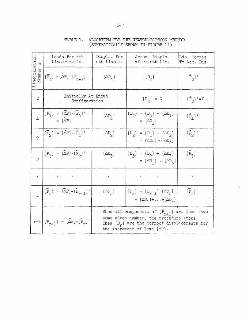
~ 0
'M -j...:> ~ cO N H
or! (J) H,..o
~ @ c:z;
'M H
0
1
2
3
r
r+l
147
TABLE 1. ALGORITEM FOR THE NEWTON-RAPHSON METHOD (SCHEMATICALLY SHOWN IN FIGURE 11)
Loads For nth Displs. For Accum. Displs. Ldso Corres. Linearization nth Linear. After nth Lin. To Acc. Dis.
(1' ) = (&) ~ (P l) n n-(till ) n (D ) n
(P ) i n
Initially At Known (DO) = 0 (P ) i =0 ·Configurc1tion 0
(1'1} = (~}_(PO}i (tilll ) (Dl } = (DO} + (Lill1 ) (P ) i
(.6P} (lill1 } 1
= =
£'1' } = (6P}-(Pl }I (lill2
) (D2) = (Dl } + (Lill2
) (P } i 2 2
(Lill~ 1 +. (lill~ 1 = 1.- e:-
(1'3} = (6P}-(P2
}v (till3
) (D3
} = (D2) + (lill3) (P } 1
3 = (,6.1)1}+ 0 + (till3)
(P } = (6P}- (Pr - l } i (Lill ) (D ) = (Dr_l)+(Lillr ) (P J f r r r r
= (Lilll)+··o+(Lillr )
When all components of (Pr +l } are less than
(Pr +l } '" '" some given number) the procedure stopso
= (6P}-(P }~ Then (D } are the correct displacements for r r the i,ncrement of load (.6P) 0
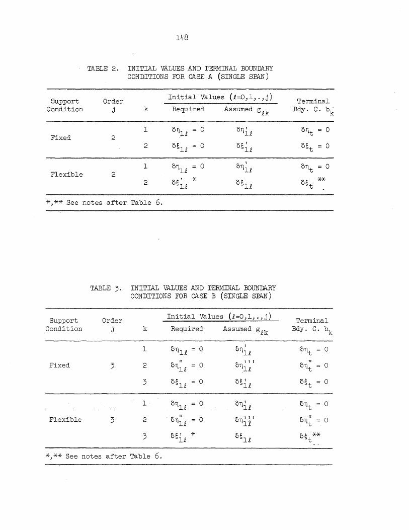
11+8
TABLE 2. INITIAL VALUES AND TERMINAL BOUNMRY CONDITIONS FOR CASE A (SINGLE SPAN)
Support Order Initial Values (£=O,l,.,j) Terminal Condition j k Required Assumed g£k Bdy. c. bk
1 O·~l£ = 0 0111£ 011t = 0 Fixed 2
2 o~l£ = 0 O~~£ O~t = 0
1 0111 £ = 0 ,
011 t OTjl£ = 0 Flexible 2
2 O~~£ * o~l£ O~t **
*,** See notes after Table 6.
TABLE 3. INITIAL VALUES AND TERMINAL BOUNMRY CONDITIONS FOR CASE B (SINGLE SPAN)
Support Order Initial Values (£=O,l,o,j) Terminal Condition j k Required Assumed g£k Bdy. C. bk
1 011 11 = 0 ,
0111 £ 011t = 0 II o "r II
Fixed 3 2 0111 £ = 0 111 £ 011t = 0
3 o~l£ = 0 o~i£ O~t = 0
1 0111 £ = 0 0111 £ 011t = 0
Flexible 3 2 " 0111 £ = ° 011' r r 11
o II
. 11t = 0
3 0~1£ * o~l£ o~ ** t
*,** See notes after Table 6.
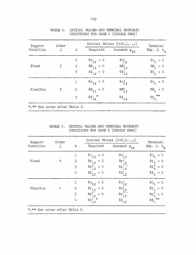
149
TABLE 4. INITIAL VALUES AND TERMJNAL BOUNDA.RY CONDITIONS FOR CASE C (SINGLE SPAN)
Support Order Initial Values ~£=O,l, .,j) Terminal
Condition j k Required Assumed g£k Bdy. Co bk
1 0111 £ = 0 o11i£ 011t = 0
Fixed 3 2 OM1 £ = 0 OMit OMt 0
3 oSl£ = 0 oS1£ OSt 0
1 0111 £ = 0 0111 £ 011 t = 0
Flexible 3 2 OM1 £ = 0 OMit OMt = 0
3 051£ * oSl£ Os ** t_
*,** See notes after Table 6.
TABLE 5. JJirITIAL VALUES AND TERMINAL BOUNDA.RY CONDITIONS FDR CASE D (SINGLE SPAN)
Support Order Ini t ial Value s (£=O,l,.,j) Terminal Condition j k Required Assumed g£k Bdy. C. bk
1 0111 £ = 0 011~.e O71t = 0
Fixed 4 2 oy 1£ = 0 oyi.e ort = 0
3 oy" = 0 o r I I Oy~1 = 0 y-, " 1£ - ..Ll "t
4 oSl£ = 0 osi£ CSt = 0
1 0711 £ = 0 0111£ 011t = 0
Flexible 4 2 oy 1£ = 0 orl £ ort = 0
3 or" 1£ = 0 o 11 ,
Yl £ oyli t = 0
4 5s1 £ * oSl£ Os ** t
*,** See notes after Table 6.
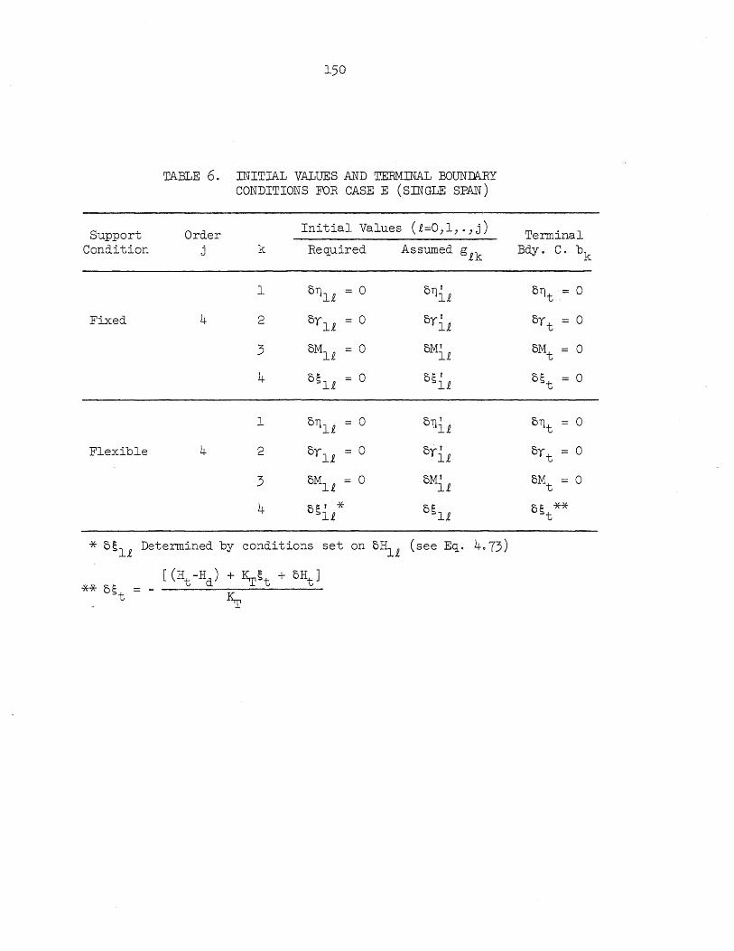
150
TABLE 6. INITIAL VALUES AND TERMINAL BOUN~RY CONDITIONS FOR CASE E (SINGLE SPAN)
Support Order Initial Values (£=O"l"o"j) Terminal Condition j k Required Assumed g£k Bdy. C. bk
1 OTjl£ = 0 0111£ OTjt = 0
Fixed 4 2 oy 1£ = 0 OY1£ OYt = 0
3 OM1£ = 0 OMit OMt = 0
4 o~l£ = 0 0~1£ OSt = 0
1 OTjl£ = 0 011i£ OTjt = 0
Flexible 4 2 oy 1£ = 0 OY1£ OYt = 0
3 OM1 £ = 0 OMit OMt = 0
4 o~r * 1£ o~l£ o~ ** t
* OSl£ Determined by conditions set on OH1£ (see Eq. 4.73)
** os [(Ht-Hd) + KT~t + OHt ]
t KT
Case
A
B
C
D
E
151
TABLE 7. DISPLACEMENT QUANTITIES USED IN IMPOSING FICTITIOUS
Case
A
c
D
E
BOUND\RY CONDITIONS AT SUPPRESSION POINTS
Oomponents of Vector Order
j b.el b.e2 b.e3
2 oT) Os
3 oT) oT)" o~
3 OT) oM 5~
4 oT) oy oy"
4 OT) oy oM
TABLE 8. EQUATION NUMBERS FOR DETERMINING LOADS Pv AND PH
(b1
}
ECl. No. for ECl. No. for Determining Pv Determining PH
4.28 4.29
4·31 4.29
4.34 4.29
4.22 4.29
4.34 4.29
b.e4
o~
as
152'
TABLE 90 DISPLACEMENTS FOR PROBLEM 1.1 (SEE SEC. 5·1.1)
Hor. Displ~ (ft) Vert. Displ. (ft) k
Discrete Cantin. Discrete Cantin.
0 0 0 0 0 1 -20107 -2.129 6.164 6.198 2 -2.558 -2.588 7·905 7·933 3 -2.007 -2.038 4.879 4.867 4 -1.536 -1.563 · -0.706 0.672 5 -1.406 -1.430 -2.318 -2·368 6 -1.447 -1.469 -4.151 -4.205 7 -1.486 -1.506 -4 0619 -4.841 8 -1.356 -1·372 -4.670 -4.305 9 -0.905 -0·914 ~2.639 -2.662
10 0 0 0 0
H = 141230 kips (discrete) H = 141200 kips (cantin. )
TABLE 10. DISPLACEMENTS FOR PROBLEM 1.2 (SEE SEC. 5.1.2)
Hor. Displ. (ft) Vert. Displ. (ft) k
Discrete Cantin. Discrete Cantin.
0 0 0 0 0 1 -·347 -·346 1.887 1.882 2 -0473 -0472 3.414 3·405 3 -.421 -.420 4.537 4.526 4 - .243 -.242 5.226 5.213 5 0 0 5.458 5.445 6 +.243 +0242 5.226 5·213 ry +.421 +.420 4.537 40526 (
8 +.473 +.472 3.414 3.405 9 +·347 +·346 1.887 1.882
10 0 0 0 0
H = 165830 kips (discrete) H = 165840 kips (cantin. )
153
TABLE 110 DISPLACEMENTS AND MOMENTS FOR PROBLEM 2.1 (SEE SEC. 5.2.1)
Hor. Disp1. (ft) Vert. Disp1. (ft) Moment (ft-k) k
Discrete Cantin. Discrete Cantin. Discrete Cantin.
0 0 0 0 0 0 0 1 -.157 -.155 0.850 0.844 6419. 6381. 2 -.226 -.223 1.596 1.583 10350. 10490. 3 -.208 -.206 2.l70 2.153 12800. 12594. 4 -.122 -.121 2·530 2·510 14120. 13912. 5 0 0 2.652 2.631 14489. 14335. 6 .122 .121 2·530 2.510 14120. 13913· 7 .208 .206 2.170 2.154. 12800. 12597· 8 . 226 .224 1.596 1·585 10350. 10208 . 9 .157 .155 0.850 0.844 6419. 6318.
10 0 0 0 0 0 0
H = 17504 kips; Shear (k=O) = 43.85 kips (discrete) H = 17510 kips; Shear (k=O) = 54.78 kips (cantin .)
TABLE 12. DISPlACEMENTS .AND MOMENTS FOR PROBLEM 2.2 (SEE SEC. 5.2.2)
Hor. Cable Di:~I". (1'1,) Vert. Cable Displ. (ft) Vert. Deck Def1. (ft) Moment (ft-k) k ._------------_._-- -----------
Discrete C( lIt t. ill, DL:3Cl'CtC Contino Discrete Contino Discrete Contino --~-----------.-.- -_._-------
0 0 0 0 0 0 0 0 0 1 -.138 .- .135 0·797 0·797 0.880 0.880 7659. 7482. 2 -.219 -0216 1.585 1.580 1.643 1.637 10916. 10716. 3 -.206 -.203 2.184 2.175 2.222 2.213 13013· 12829. 4 -0122 ~o120 20558 20546 2.583 2·571 14160. 13990. 5 0 0 2.684 2.672 2·706 2.693 14538. 14367· 6 +0122 +0121 2.558 2.547 2·583 2·572 14160. 13997· 7 +.206 +0204 2.184 2.177 2.222 2.214 13013· 12849· 8 +.219 +.216 10585 1.582 1.642 1.639 10916. 10794. \-'
9 +0138 +·+35 0·797 0·798 0.880 0,882 7659. 7540. \Jl +=-
lO 0 0 0 0 0 0 0 0
H = 17500 kips; Shear (k=O) = 52010 kips (discrete) H = 17500 kips; Shear (k=O) = 160.0 kips (continuous)
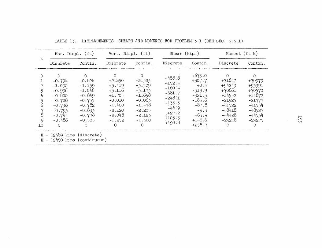
TABLE 13. DISPLACEMENTS) SHEARS AND MOMENTS FOR PROBLEM 3.1 (SEE SEC. 5.3.1)
Hor. Disp1. (ft) Vert. Disp1. (ft) Shear (kips) Moment (ft-k) k
Discrete Contino Discrete Contino Discrete Contino Discrete Contino
0 0 0 0 0 +488~8
+675.0 0 0 1 -0·794 -0.826 +2.250 +2.323 +152.4 +307·7 +71847 +70979 2 -1.092 -1.139 +3·419 +3·509 -160:4 +0·5 +94243 +93391 3 -0.996 -10048 +3·116 +3·173 -381:7 -319·9 +70661 +70570 4 -0.800 -0.849 +1.704 +1.698
~248~1 -321·3 +14552 +14872 5 -0.708 -0·755 -0.010 -0.063
-133: 3, -185.6 -21925 -21777
6 -0·738 -0.782 -10400 -1.478 746:9 -87·8 -41522 -41534 7- -0·793 -0.833 -2.120 -2.205 -9·3 -48418 -48527 8 -0·744 -00778 -2.048 -2.123 +27·2 +63·9 -44428 -44534
+lq3~5 1--1
9 -0.486 -0·505 -1.252 -1·300 +146.6 -29218 -29275 Vl
+198."8 Vl
10 0 0 0 0 +258·7 0 0
H = 12389 kips (discrete) H = 12450 kips (continuous)
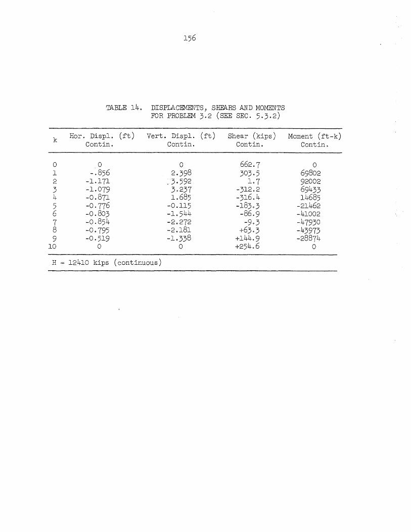
TABLE 14. DISPLACEMEN"TS) SHEA.RS AND MOIY1ENTS FOR PROBLEM 3.2 (SEE SEC. 5.3.2)
k Hor. Disp1. (ft) Vert. Disp1. (ft) Shear (kips) Moment (ft-k) Contino Contino Contino Contino
0 0 0 662.7 0 1 -.856 2·398 303·5 69802 2 -1.171 ~3· 592 1·7 92002 3 -1.079 3·237 -312.2 69433 4 -0.871 1.685 -316.4 14685 5 -0·776 -0.115 -183.3 -21462 6 -0.803 -1.544 -86·9 -41002 7 -00854 -2.272 -9·3 -47930 8 -0·795 -2.181 +63.3 -43973 9 -0·519 -1·338 +144·9 -28874
10 0 0 +25'4.6 0
H = 12410 kips ( cont inuous )
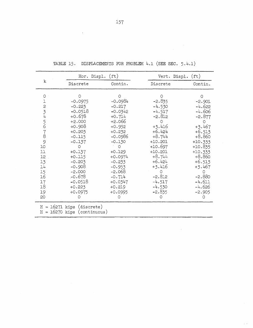
157
TABLE 15. DISPLACEMENTS FOR PROBLEM 4.1 (SEE SEC. 5.4.1)
Hor. Disp1. (ft) Vert. Disp1. (ft) k Discrete Cantin. Discrete Cantin.
0 0 0 0 0 1 -0.0975 -0.0984 -2.835 -2·90~ 2 -0.223 -0.217 -4·530 -4.622 3 -0.0518 -0.0342 -4.517 -4.606 4 +0.678 +0·714 -2.812 -2.877 5 +2.000 +2.066 0 0 6 +0·908 +0·952 +3·416 +3·467 7 +0.203 +0.232 +6.424 +6.513 8 -0.115 -0.0986 +8·744 +8.860 9 -0,137 -0.130 +10.201 +10·333
10 0 0 +10.697 +10.835 11 +0.137 +0.129 +10.201 +10·333 12 . +0.115 +0.0974 +8·744 +8.860 13 -0.203 -0.233 +6.424 +6.513 14 -0.908 -0·953 +3·416 +3·467 15 -20000 -2.068 0 0 16 -0.678 -0·714 -2.812 -2.880 17 -0.0518 +0.0347 -40517 -4.611 18 +0.223 +0.219 -4·530 -4.626 19 +000975 +0.0995 -2.835 -2·905 20 0 0 0 0
H = 16271 kips (discrete) H = 16270 kips (continuous)
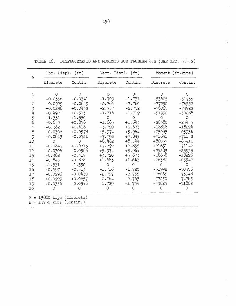
TABLE 16. DISPIACEMENTS AND MOMENTS FOR PROBLEM 4.2 (SEE SEC. 504.2)
Hor. Displ. (ft) Vert. Displ. (ft) Moment (ft-kips) k
Discrete Cantin. Dif3crete Cantin. Discrete Cantin.
0 0 0 Oi, 0,.: 0 0 1 -0.0356 -0.0341 -1·729 -1·731 -53625 -51735 2 -0.0929 -0.0849 -20764 -2.760 -77250 -74532 3 +000296 +0.0432 -2·757 -2.752 -76065 -73922 4 +0.497 +0.513 -1·716 -1·719 -51992 -50288 5 +1·331 +1·350 0 0 0 0 6 +0.845 +0.878 +1.683 +1.643 -26380 -25445 7 +0.382 +0.418 +3~720 +3.673 -18838 -18224 8 +0.0306 +0.0578 +5.974 +5.964 +25283 +23934 9 -0.0843 -0.0721 +7·792 +7.835 +71651 +71142
10 0 0 +8.482 +8.544 +86057 +85911 11 +0.0843 +0.0713 +7·792 +7·835 +71651 +71142 12 -0.0306 -0.0586 +5.974 +5.964 +25283 +23933 13 -0.382 -0.419 +3·720 +3·673 -18838 -18226 14 -0.845 -0.878 +1.683 +1.643 -26380 -25547 15 -1.331 -10350 0 0 0 0 16 -0.497 -0·513 -1.716 -1·720 -51992 -50306 17 -0.0296 -0.0430 -2·757 -2:755 -76065 -73948 18 +0.0929 +0.0857 -2.764 -2.763 -77250 -74785 19 +0.0356 +000346 -1·729 -1·734 -53625 -51862 20 0 0 0 0 0 0
H = 13880 kips (discrete) H = 13750 kips (cantin. )
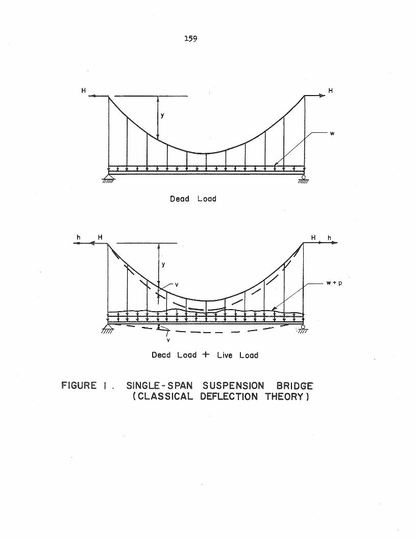
159
H H
w
Dead Load
h H H h
v
Dead Load + Live Load
FIGURE I. SINGLE-SPAN SUSPENSION BRIDGE (CLASSICAL DEFLECTION THEORY)
w+p
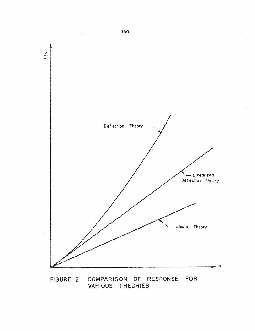
p w
160
Deflection Theory
Linearized Defle ction Theor y
- Elastic Theory
FIGURE 2. COMPARISON OF RESPONSE FOR VARIOUS THEORIES
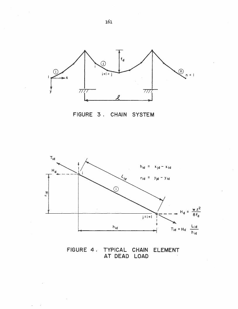
y 1111
~I 1111
I~
FIGURE 3. CHAIN SYSTEM
rid = Yjd - Yid
FIGURE 4. TYPICAL CHAIN ELEMENT AT DEAD LOAD
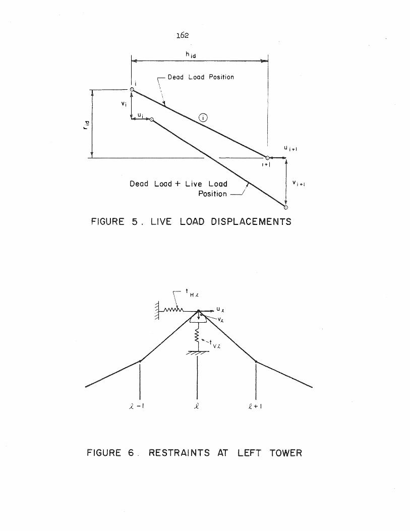
Vi
\ Dead Load Position
Dead Load + Live Load Position -I'
U i-rl
FIGURE 5. LIVE LOAD DISPLACEMENTS
\ t H..t
)-1 £+1
FIGURE 6. RESTRAI NTS AT LEFT TOWER
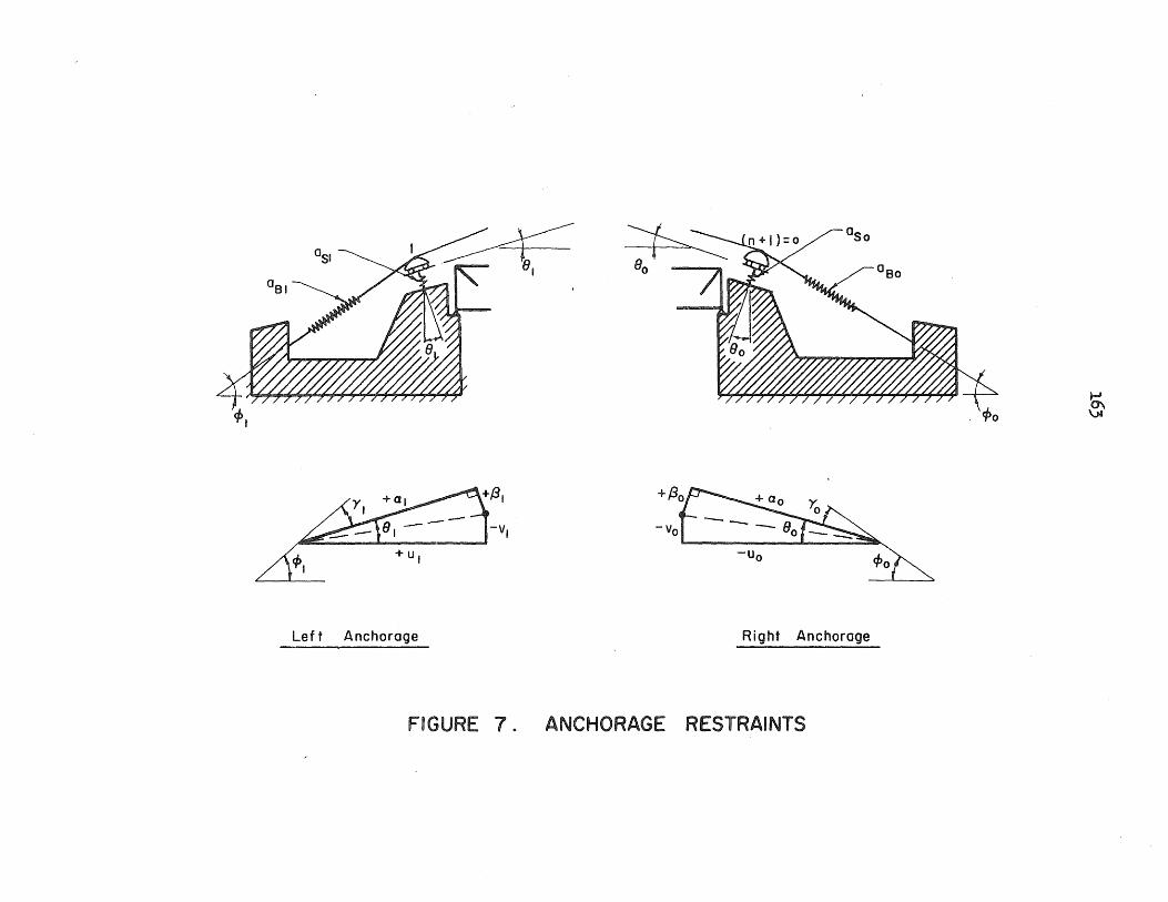
~
-VI . 1i"""'"""' /
4>1 + u, -uo
Left Anchorage Right Anchorage
FIGURE 7 e ANCHORAGE RESTRAINTS
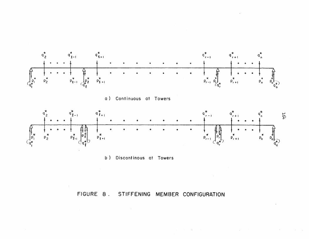
.". * « *" "* * q2 q ~-I q 9.+ I qr-I qr+1 qn
• iii iii 1\1 1\1 e e ED ED a. & III • e
• e ED " • III • e III G f
P~ t • • •
* * "* * * * * P2 PQ- 1 . PR P~ +1 Pr- I Pr + 1 Pn (q*, q~
a ) Cont inuous at Towers
*' * * * *' q* q2 q R-I q t + 1 qr-I qr+1 I-' n ~ G • III ! ,
• G • «I III e 4& CD CD CD
III CD • T Jill t • III • e III CD III III CD CD
*' * pi-I pr ~ * * "* P P2 Pl +1 Pr- I Pr +1 Pn Po /1 I CqllE' qg) '*
I qo
b ) Discont inous at Towers
FIGURE 8. STIFFENING MEMBER CONFIGURATION
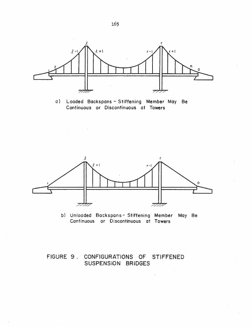
a) Loaded Backspans - Stiffening Member May Be Continuous or Discontinuous at Towers
b) Unloaded Backspans - Stiffening Member May Be Continuous or Discontinuous at Towers
FIGURE 9. CONF'IGURATIONS OF STIFFENED SUSPENSION BRIDGES
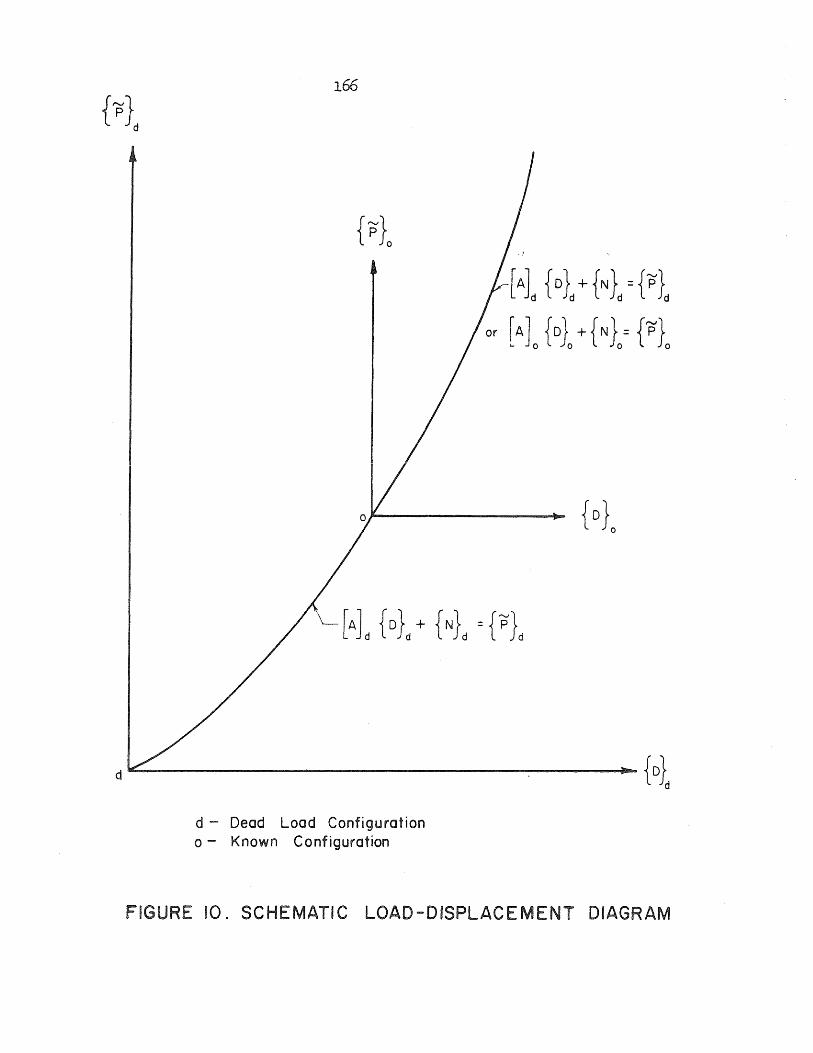
-f
[~d {D}d + {N}d = {P}d
He {Dl +{N1= {p}e
{o} o
d~------------------~{0 d
d - Dead Load Configuration o - Known Configuration
FIGURE 10. SCHEMATIC LOAD-DISPLACEMENT DIAGRAM
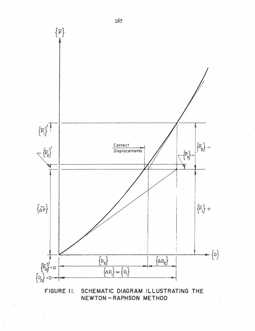
{~{r Correct ~-}
J.r-.J}I Displacements Ji 1 t2-~ ___ -----+-llf+----~1.P3J- '
FIGURE II. SCHEMATIC DIAGRAM ILLUSTRATING THE NEWTON - RAPHSON METHOD
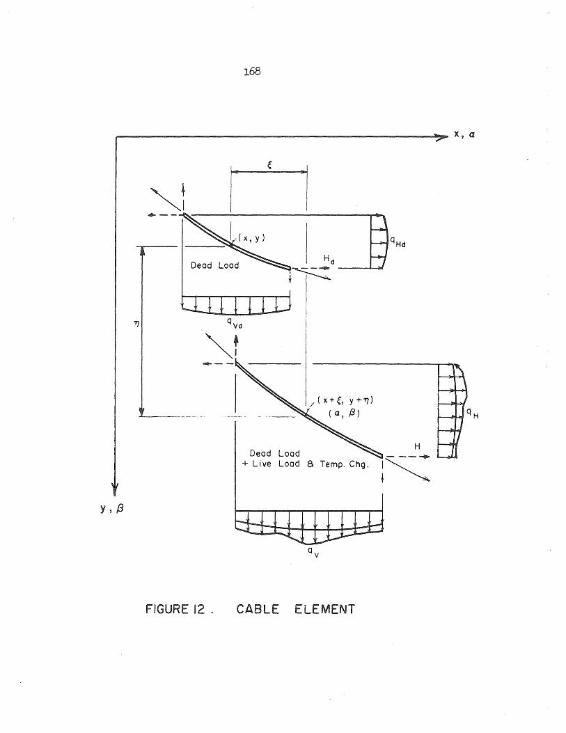
y,{3
168
41- - -~.------------__ ....
Dead Load
..... --
/ ( X + e, y + 7])
( a, (3)
H Dead Load
+ live Load 8 Temp. Chg. !~
FIGURE 12 . CABLE ELEMENT
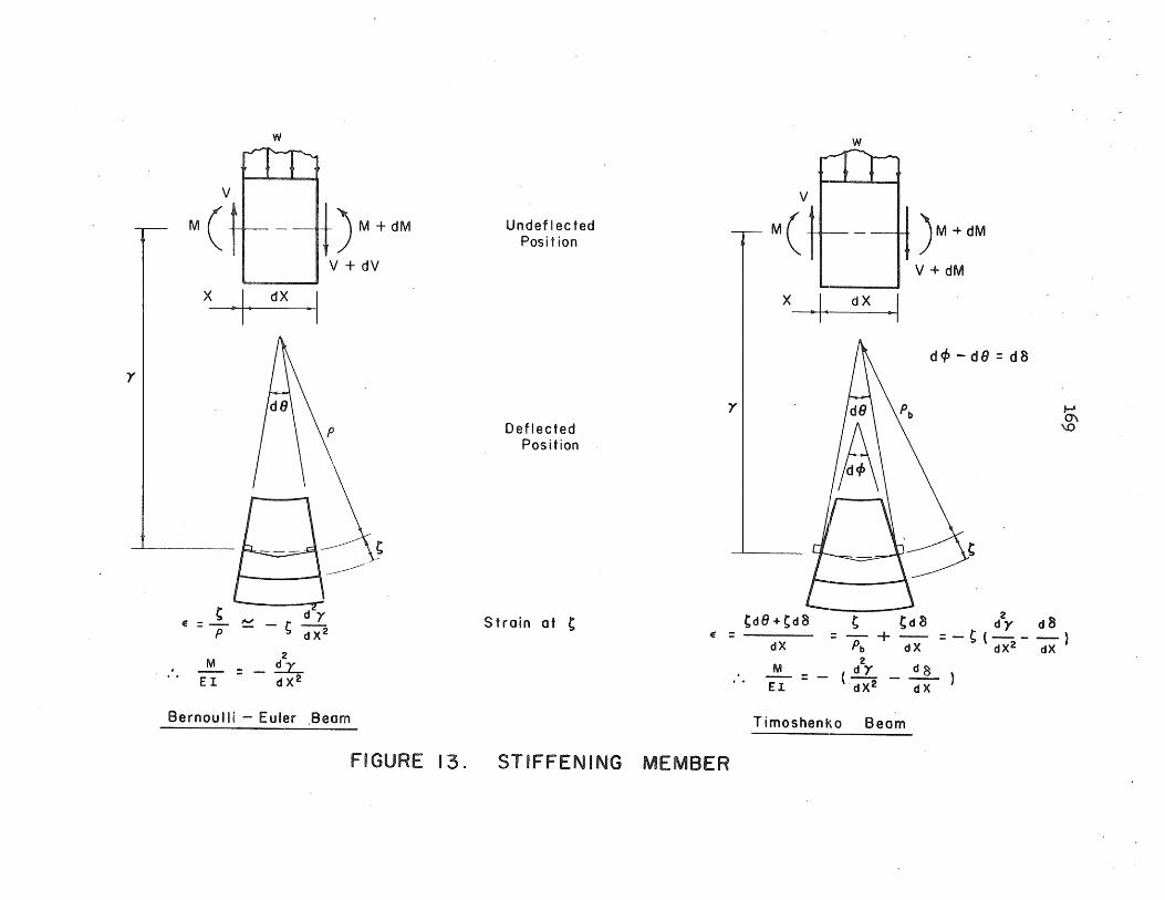
w w
~ ~
~ tV d )" E = p. - ~ dX 2
2
~= ~ E I d X2
Strain at C 2 Cd8+Cd8 ~ ~d8 d)" d8
=-+- =-~(---) Pb dX dX 2 dX
2 M d Y d 8
U = ( dX 2 - -;;x-
E =
Bernoulli - Euler ,Beam Timoshen.~o Beam
FIGURE 13. STIFFENING MEMBER
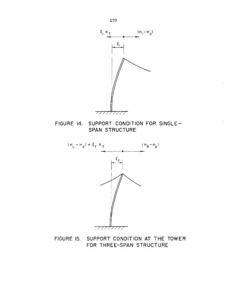
170
" KT (H1-H d) _&!!I(i---__..I11----'lllo-
FIGURE 14. SUPPORT CONDITION FOR SINGLESPAN STRUCTURE
~-.----------. ~-----~
FIGURE 15. SUPPORT CONDITION AT THE TOWER FOR THREE-SPAN STRUCTURE
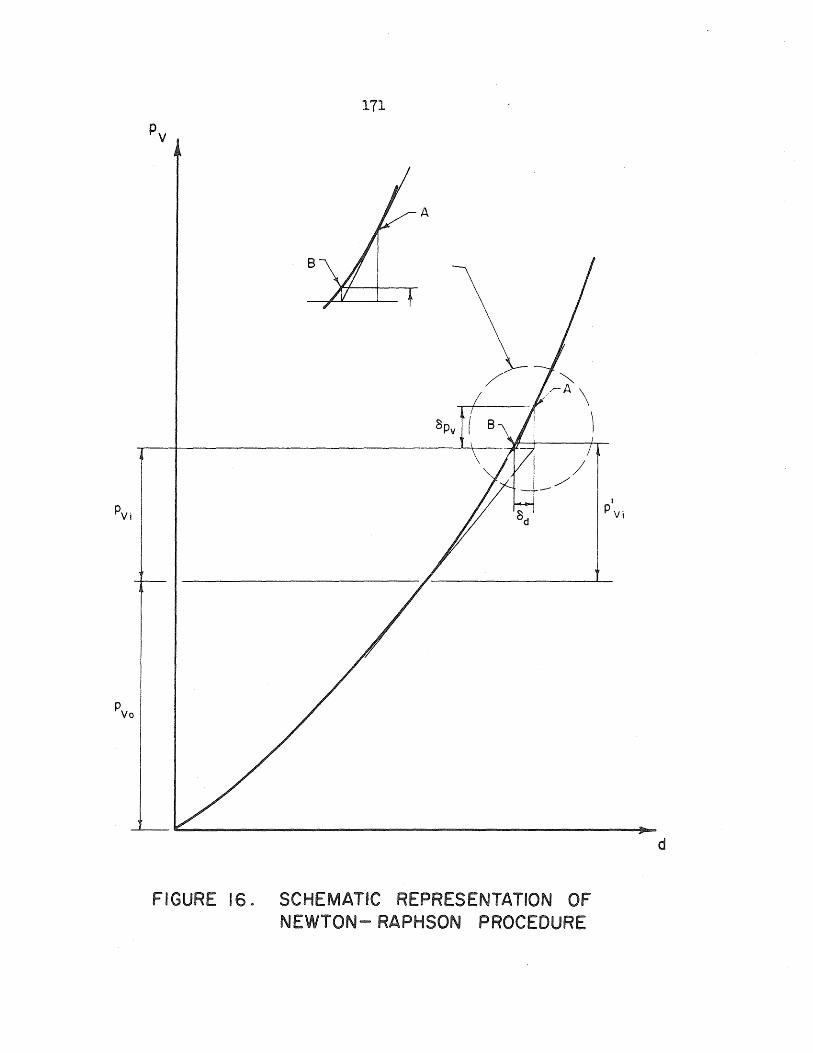
171
A
FIGURE 16. SCHEMATIC REPRESENTATION OF NEWTON- RAPHSON PROCEDURE
d
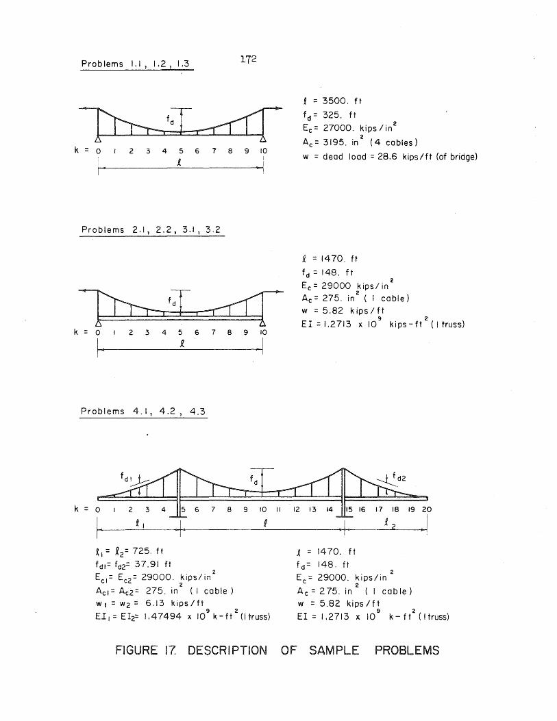
Prob lems I. I, 1.2, 1.3 172
k = 0 2 3 4 5 6 7 8 9 10
I · £ ~l
Problems 2.1,2.2,3.1,3,2
k = 0 2 3 4 5 6 7 8 9 10
I, ;. p I
Problems 4. I, 4,2, 4.3
k = 0
1---------'------+. /----
~I= X2= 725. ft
f dl = fd2= 37.91 ft
Ecl = Ec2 = 29000. kips/in2
2 Acl= Ac2= 275. in (I coble)
WI = w2 = 6.13 kips 1ft
10 II
9 2 Ell=EI2=1.47494xI0 k-ft (I truss)
f = 3500. ft
fd= 325. ft
Ec = 27000. kips I in2
2 Ac = 3195. in (4 cables)
w = dead load = 28.6 kips/ft (of bridge)
~ = 1470. ft
f d = 148. f t 2
Ec = 29000 k ips I in 2
Ac = 275. in (I cable)
w = 5.82 k ips 1ft 9 2
EI=I,2713 )( 10 kips-ft (I truss)
.( = 1470. ft
fd= 148. ft Ec = 29000. kips/in 2
2 Ac= 275. in (I cable)
w = 5.82 kips 1ft 9 2
EI = 1.2713 x 10 k-ft (Itruss)
FIGURE 17 DESCRIPTION OF SAMPLE PROBLEMS
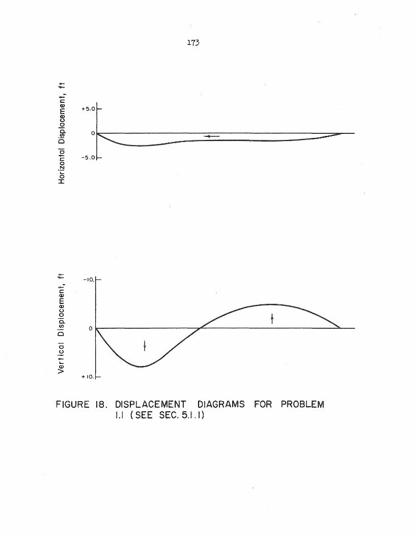
173
-'+-
-C w +5.0 E w (,)
.52 0- 0 .~ 0
0 - -5.0 c 0 -~ ~
0 :r:
-...... -10.
-C w E w (,)
0 t 0-W 0 0
0 (,) -~ W >
+ 10.
FIGURE 18. DISPLACEMENT DIAGRAMS FOR PROBLEM 1.1 (SEE SEC. 5.1. I)
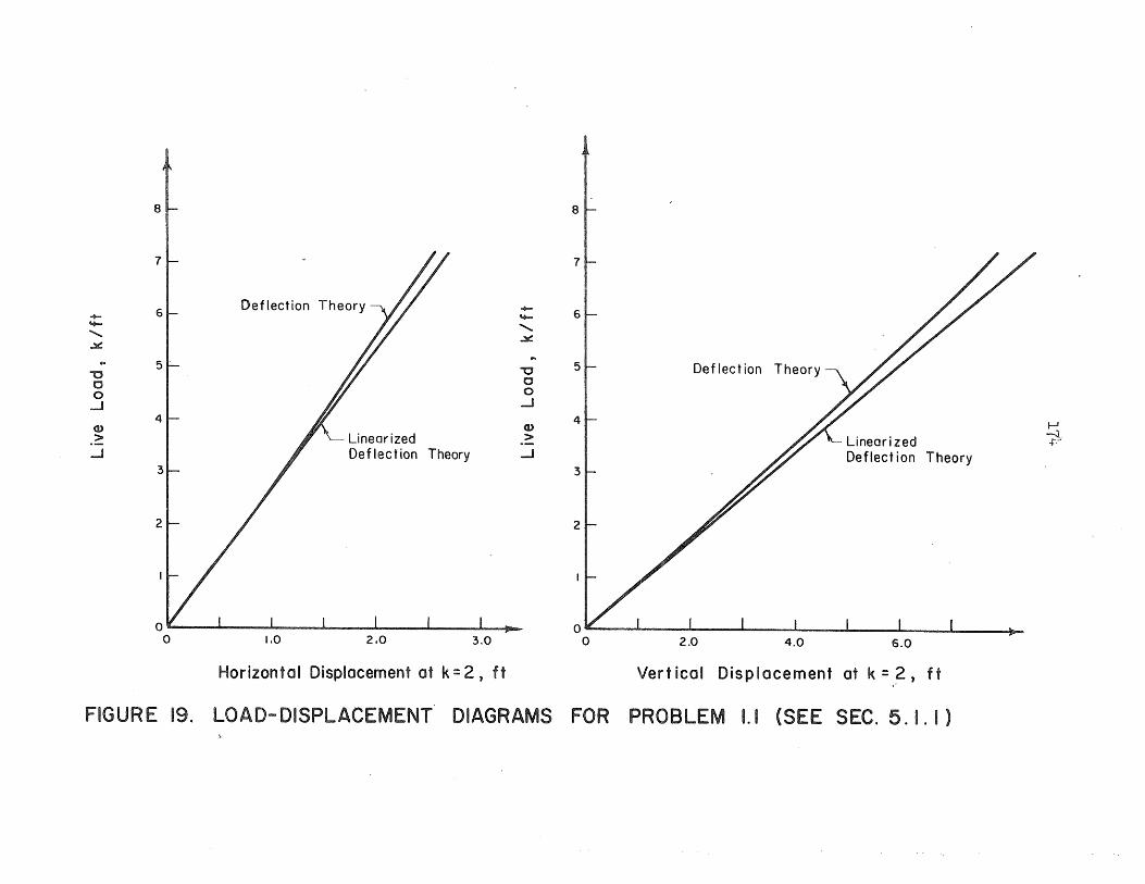
:r 8
7
l Deflection Theory - 6 - 'i-
'i- , , ..lI::
..lI::
5 "0 5t- Deflection Theory "'0 0 0 0 0 ...J ...J
4 4 f-' OJ Q)
~, ?: > ~ Linearized ...J Theory ...J Deflect ion Theory
3 3
2 2
ow ~
o 1.0 2.0 3.0 ow ~
o 2.0 4.0 6.0
Horizontal Displacement at k = 2, ft Vertical Displacement at k =.2, ft
FIGURE 19. LOAD-DISPLACEMENT DIAGRAMS FOR PROBLEM 1.1 (SEE SEC. 5.1. I)
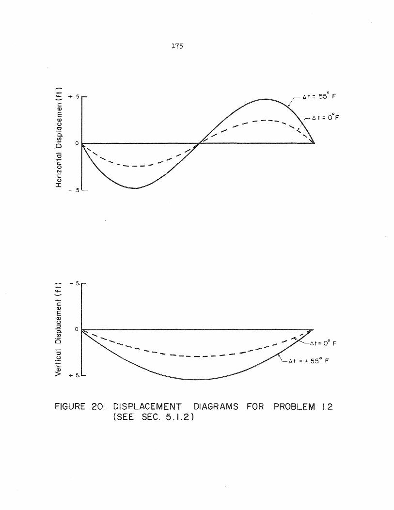
-'+- +.5
c CD
E CD u c a. cJ)
,0
c -c o N
"-o I
--'+-
-C CD E Q,) u c 0.. cJ)
Ci
c u -"-CD >
- .5
-T 0
+ 5.
175
o r- t:. t = 55 F
/
o ,r-6t=OF
FIGURE 20. DISPLACEMENT DIAGRAMS FOR PROBLEM 1.2 (SEE SEC. 5. I. 2 )
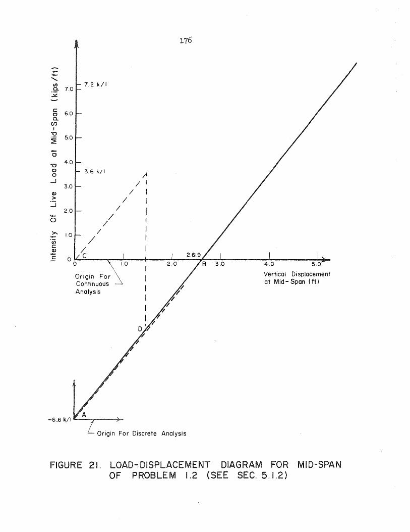
--"tao
........ (/) 7.2 k/ I a. 7.0 ~
c c 6.0 a.
(/') I
"'C :E 5.0
-C
"'C 4.0 C o 3.6 k/ I
..J
C1> > ..J
..... o
3.0
2.0
~ 1.0 (/)
c.::: C1> -c.:::
/ o / C
o
/ /
/
/
;1 /1
/ I / I
/ I
Origin For ~ Continuous Analysis
Origin For Discrete Analysis
4.0 50
Vertical Displacement at Mid - Span (ft)
FIGURE 21. LOAD-DISPLACEMENT DIAGRAM FOR MID-SPAN OF PROBLEM 1.2 (SEE SEC. 5.1.2)
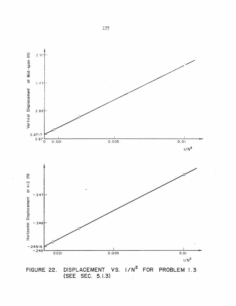
- 29+ -c 0 a. tn I
-0
~
-0
C <U E <U 0 0 Ci tn
0 "0 u -.~ <U >
(\J 1\ .It:
-o
C <U E Q)
u o a. tn
o
2 83
288
2.8717 2.87
-.247
o -.246 C o N ~
o ::r:
-.24516
I I I I
.-
a
177
... /
0.001 0.005 0,01
I/N 2
-.245~--~--~--------------~------------------------~----~
0.001 0.005 0.01
I/N2
FIGURE 22. DISPLACEMENT VS. I/N2 FOR PROBLEM 1.3 (SEE SEC. 5.1.3)
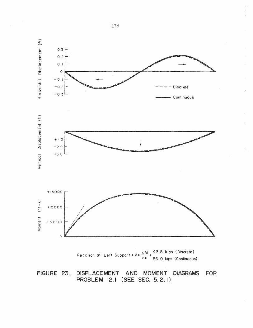
---c: <1>
E <1> u 0 a. <n
0
0
c: 0 N
'-0 I
C <lJ
E Cl> u o a. \/)
Ci
-0 u
.:JC !
0,3
0,2
0, I
° -0. !
-0.2 -
-0-3
+ 15000-'·
.:: -tIOOOO
c E +500(;-o ~
178
--- - Discrete
-_ ..... Continuous
o ~--------------------------------------------------~
dM 43.8 kips (Discrete) Reaction at Lef1 Support = V= - =
d){ 56.0 kips (Continuous)
FIGURE 23. DISPLACEMENT AND MOMENT DIAGRAMS FOR PROBLEM 2.1 (SEE SEC. 5.2.1)
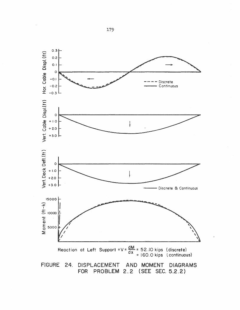
179
- 0.3 -~ 0.2 0. U') 0.1 a Q)
0
..c -0.1 -E--0
() - - - - Discrete ...: -0.2 -- Continuous 0 ::c -0.3
--~ -a. U')
0 0
Q) + 1.0 ::c 0 + 2.0 ()
.....: +3.0 ~
Q)
>
-~ -'1i> 0 0 .:::t! + 1.0 u Q)
0 +2.0 -~ Q) +3.0 > -- Discrete a Continuous
15000 - , .:z:. I - • ~ 10000 - I c Q)
g 5000
~
Reaction at Left Support =V= ~M = 52.10 kips (discrete) )( = 160.0 kips t continuous)
FIGURE 24. DISPLACEMENT AND MOMENT DIAGRAMS FOR PROBLEM 2.2 (SEE SEC. 5.2.2)
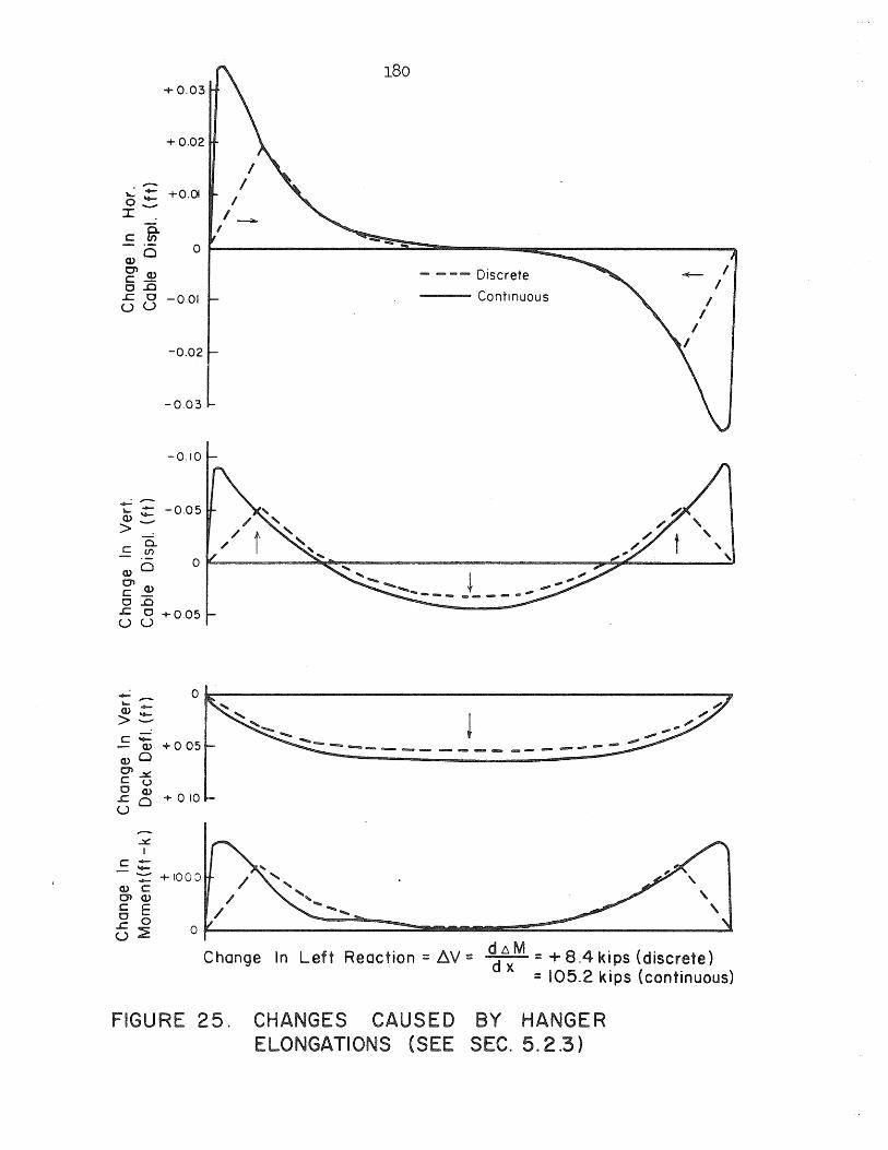
-. -0'::: I .
c fi} (1)0
~~ c..c
+0.03
+0.02
+0.01
..c 0 -0.01 UU
-0.02
-0.03
-0.10
..,..;:-'- ~ -0.05 (1)-> .
- - - -- Discrete
--...... Continuous
'\
"
I I
" c .~ w O C'JI w
O~--------~~~------------------------~~~--------~, c_ c..c ..c 0 +005 UU
- 0 '- -w->.:=:. c;::: - w +005 w o C'JI..:.;: c u c w
+ 0 10 ..co U
..:.;: I
~:: -:;:: + 100 J
w C C'JI(1)
~
C E -_ o 0 I;: ________ -=::::::=====-~ .. Ma .. ==~==::=_ ____________ ~ t3 ::E 0 ""
Change In Left Reaction = !:lV:: ~ L'l M = + 8.4 kips (discrete) x = 105.2 kips (continuous)
FIGURE 25. CHANGES CAUSED BY HANGER ELONGATIONS (SEE SEC. 5.2.3)
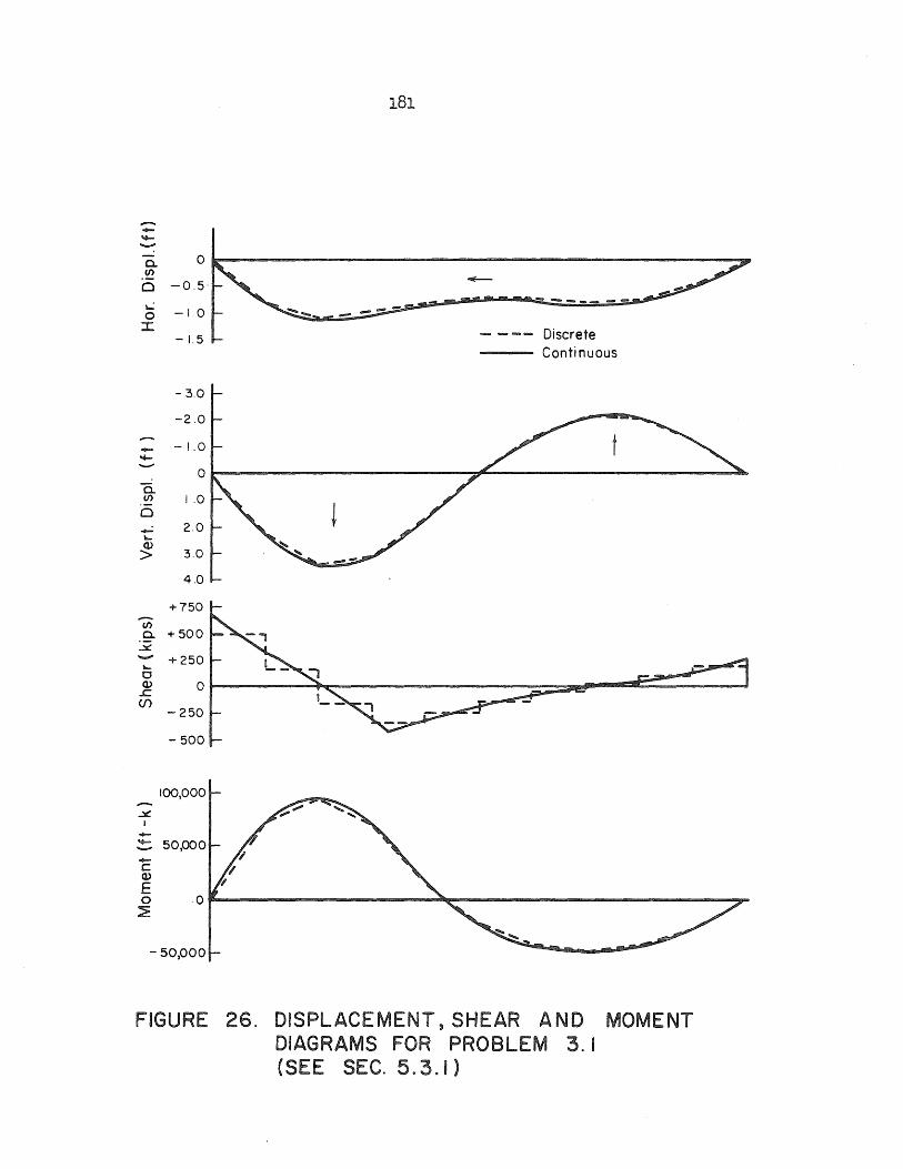
181
--~ -- 0 c. en
0 -0.5'
~ -10 0
:I: -1.5 - - - - Discrete
-- Continuous
- 3.0
-2.0
- -1.0 .... "-'"
0 C. en 1.0 0
-= 2.0 '-Q)
> 3.0
4.0
+750 -(/)
0- +500 .::a::. -'- +250 c Q) 0 .c:.
(f) -250
- 500
! loo,o°t :=. 50pOO -c
Q)
E 0 .0 ~
- 50,000
FIGURE 26. DISPLACEMENT, SHEAR AND MOMENT DIAGRAMS FOR PROBLEM 3. I (SEE SEC. 5.3.1)
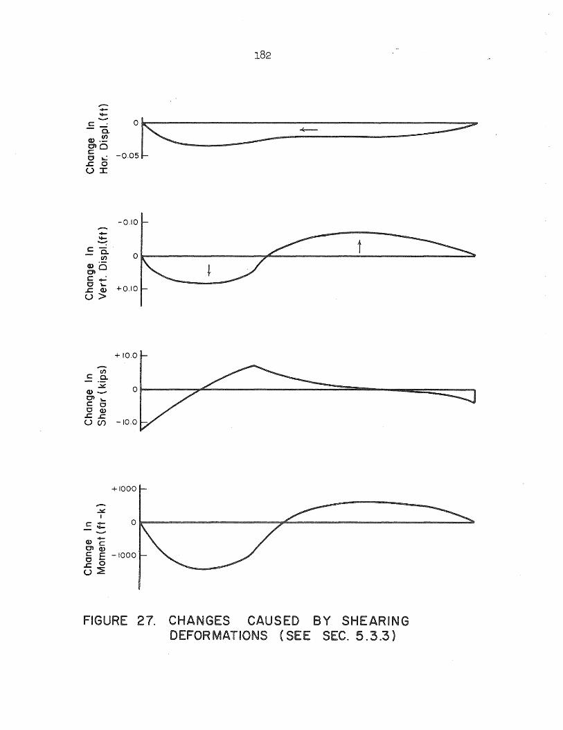
182
-0.10 --...... t -......:-
c-_ a. 0 (/)
CDO t1' C -0 '"- +0.10 .t::. CD U>
+ 10.0
-(/)
E.9-~ 0
CD -0' '"-C C C CD
.t::..t::. UCf) -10.0
FIGURE 27. CHANGES CAUSED BY SHEARING DEFORMATIONS (SEE SEC. 5.3.3)
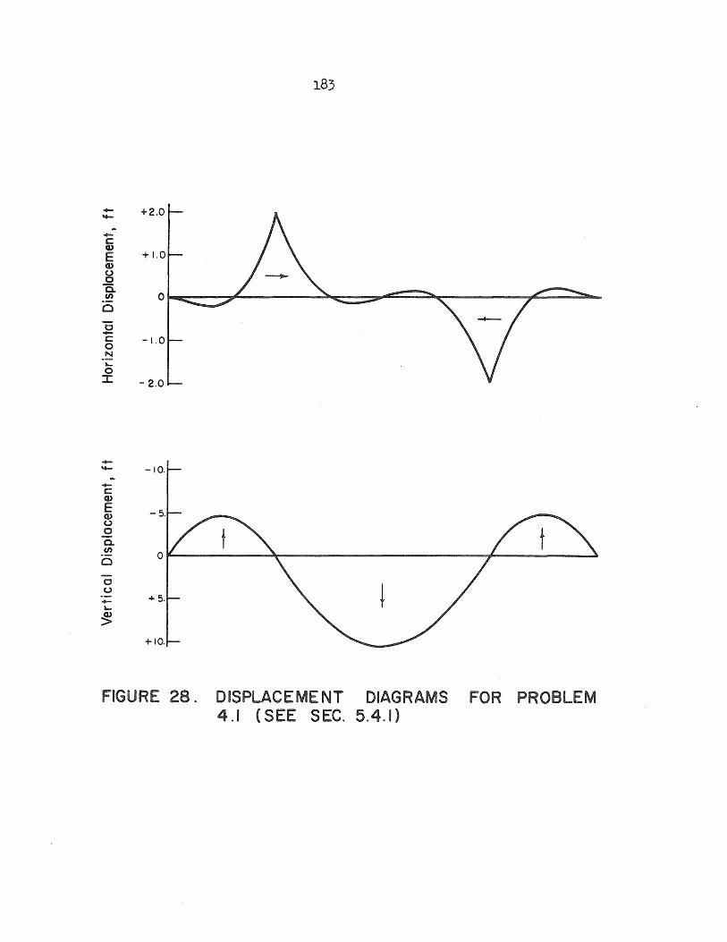
- +2.0 ...... ... -c:
CI)
E CI) 0 0 C. en 0
C
"0 -c: - 1.0 0 N
"-0 J: - 2.0
-...... -10 . ... -c: CI)
E CI) 0 0 0-en
0 C
0 0 -"-~
FIGURE 28. DISPLACEMENT DIAGRAMS FOR PROBLEM 4.1 (SEE SEC. 5.4.1)
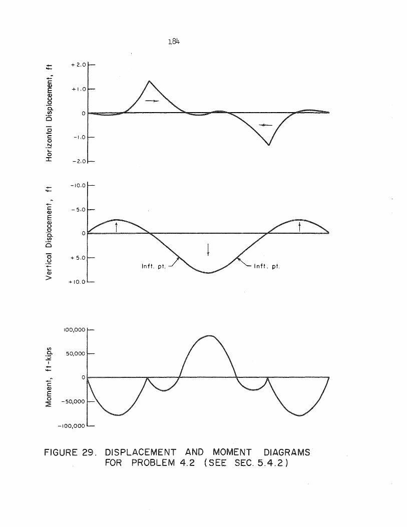
-c Q.)
E Q) u
..Q c. en o o -c o N
"-o I
-c: Q.)
E Q.) u o c. en o
o u -"-Q)
>
(/)
c. ~
I -f+-
-c: Q)
E 0 ~
184
-10,0
- 5,0
+ 5.0
Inft. pt. Inft. pt.
+10.0
100,000
50,000
0
-50,000
-100,000
FIGURE 29. DISPLACEMENT AND MOMENT DIAGRAMS FOR PROBLEM 4.2 (SEE SEC. 5.4,2)
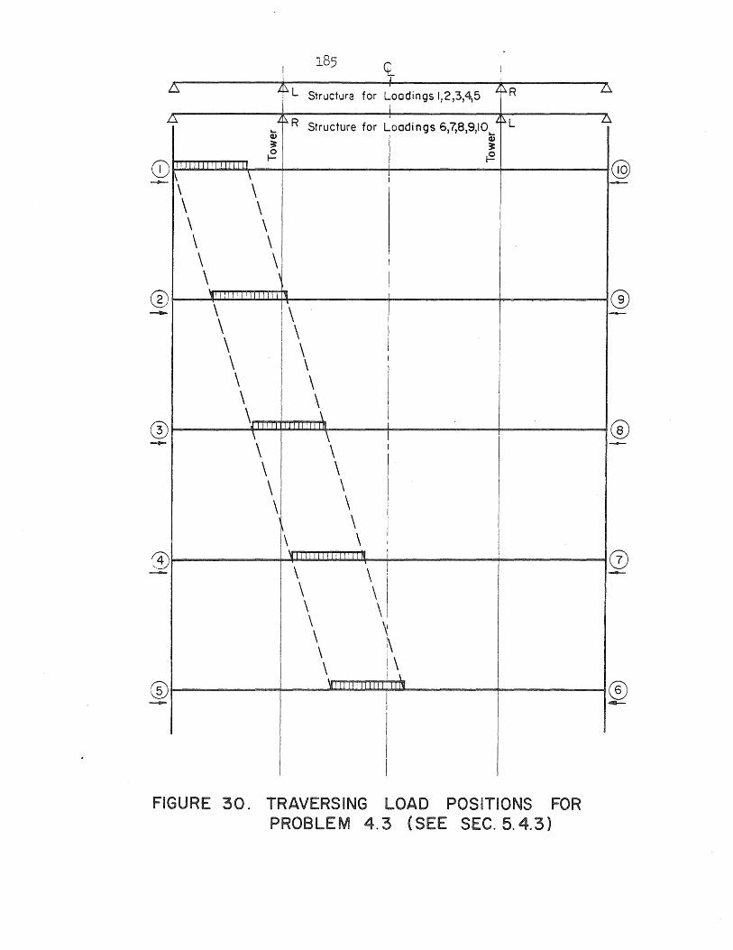
2 Structure for Loadings I, ,3,4, I
A iii R Structure for Loadings 6,7,8,9,10 L ~L L.. <l> '-
<l> ~ 3: 0
~ t-I1 I I II I II I I II I I "
\ \ I
\ \ CD -
\ \ \ \ \ \ \ \ f
\ , '1\ 111111 11
I
\ \ \ \ \ \ \ \
I
®
\ \ \ \ \ \
d 11'1 i \ \ I
\ \ I
\ \
\{ \ \ \
\ \ I
'II I 11111 I I 11111 I I "
\ \ \ \ \ \ \
~ \ !\ \ \ i\
-- '11,11111111111' Ill'll
I ®
FIGURE 30. TRAVERSING LOAD POSITIONS FOR PROBLEM 4.3 (SEE SEC. 5.4.3)
.6.
@
®
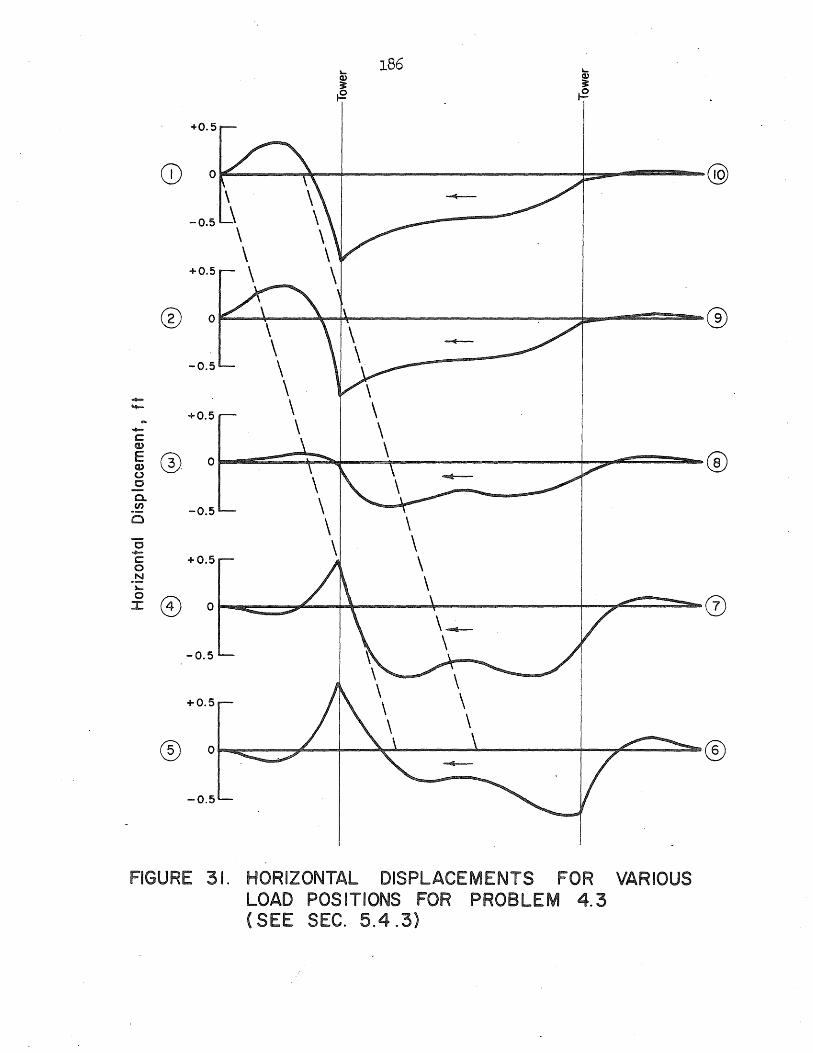
~ 186
~
Cl> Cl> !t !t ~ ~
+0.5
CD 0
-0.5
+0.5
® 0 \ \
-0.5 \ \ - \ 114-
... +0.5 \ -c:
w E ®. 0 w u 0
a. en -0.5 0 \ 0 \ -c: +0.5 \ 0
.!:::! \ "-0
® :I: 0
-0.5
+0.5
® 0
-0.5
FIGURE 31. HORIZONTAL DISPLACEMENTS FOR VARIOUS LOAD POSITIONS FOR PROBLEM 4.3 (SEE SEC. 5.4 .3)
@
®
®
(])
®
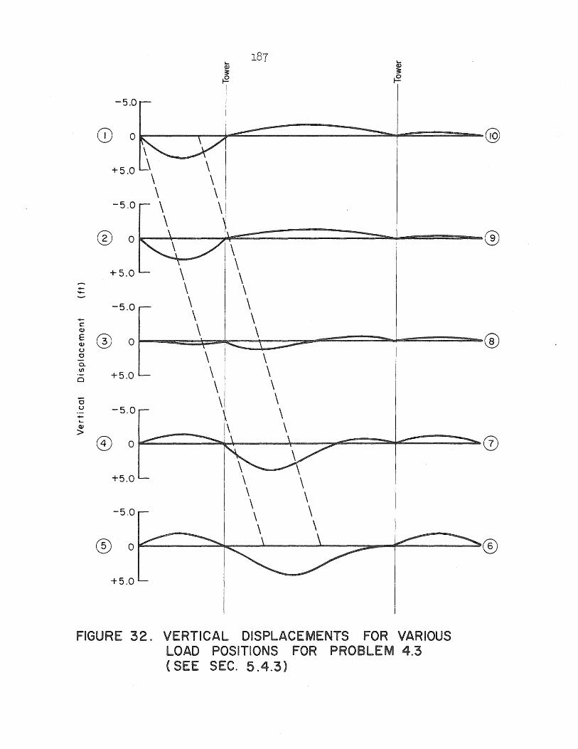
I-187 I-
Q) Q)
~ 3: ~ ..e
-5.0 I
CD 0
\
+5.0 ~ \ \
-5.0 \ \
® 0 \
+5.0 \ \ \ - \ ..- \ -- \ \ -5.0
..- \ \ c: \ C'!,) \ E ® Q) 0
u
\ c \ 0-en
\( \ +5.0 0 \
"0 \ u -5.0 \ .-..-I...
1\ \ Q)
> 8) 0
+5.0
-5.0
® 0
+5.0
FIGURE 32. VERTICAL DISPLACEMENTS FOR VARIOUS LOAD POSITIONS FOR PROBLEM 4.3 (SEE SEC. 5.4.3)
@
®
®
(j)
®
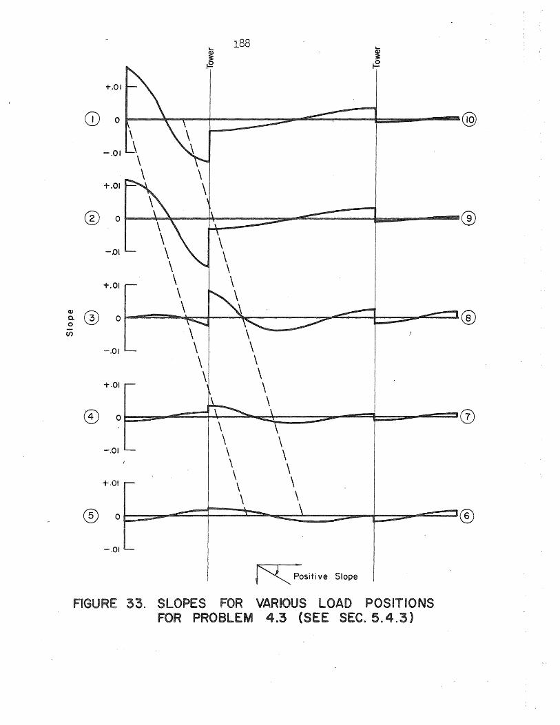
~ 188
~
Q) Q)
~ ~
~ ~
+.01
CD 0 @
-.01
+.01
® 0 ® \ \
-Dl \ \
+.01 \ \
Q)
® \
® c. 0 0
en \ -.01 \
\ \
+.01 \ \
® 0 0 \ \ \ \
-'.01 \ \ \ \ \
+.01 \ \ \ \
® 0 ®
-.oIL ~ Positive Slope
FIGURE 33. SLOPES FOR VARIOUS LOAD POSITIONS FOR PROBLEM 4.3 (SEE SEC. 5.4.3)
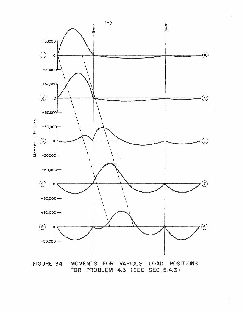
+50pOO
+50,000
® a \ \ \ \
-50,000 \ \ -;;; \ \ c. \ .:.:. +50,000 I \ --
® a c (1) \ E 0 \ ~ -50POO
\
+50,00
®
-50,000
-t-50,OOO
® 0
-50,000
FIGURE 34. MOMENTS FOR VARIOUS LOAD POSITIONS FOR PROBLEM 4.3 (SEE SEC. 5.4.3)
®
®
(])
®
APPENDIX A. COMPUTER PROGRAMS
A.l. STRESS
As mentioned in Chapter 3, STRESS is a problem-oriented
computer language for structural engineering which facilitates the use
of digital computers for structural analysis. STRESS is used in this
study only for the determination of the stiffness coefficients of the
stiffening member. The reader is referred to Fenves (1965a, 1965b)
for a complete treatment of STRESS.
The input data for STRESS includes all the information neces
sary to define the stiffening member completely. The stiffness coef
ficients are computed by subjecting each support point to a unit
displacement and determining the corresponding support reactions.
A.2. Modified Version of STRESS
In order to compute the stiffness coefficients of the
stiffening member and to perform the discrete suspension bridge analysis
in the same pass through the computer, it is necessary to modifY the
STRESS output medium. The result of this modification is that the
stiffness coefficients are placed on magnetic tape instead of being
printed out through the normal STRESS output. Control is then trans
ferred to the discrete suspension bridge program which has access to
the magnetic tape on which the stiffness coefficients are stored. These
quantities are read from the tape as they ar~ needed by the discrete
suspension bridge program.
190

A provision is included that makes it possible to output the
stiffness coefficients on binary data cards. This is useful when the
same bridge is to be analyzed for several different loading conditions.
After the initial STRESS problem is solved, these data cards are
available for subsequent runs and provide the stiffness coefficients
directly without the use of STRESS.
A.3. Program for the Discrete Analysis of Suspension Bridges
There are no unusual features in the program for the discrete
suspension bridge analysis " The program is designed to use two separate
core loads. The first core load includes all parts of the program
except the solution of the simultaneous equations, which is performed
by a Gauss elimination procedure in the second core load. This division
is dictated by storage requirements in order that large numbers of
equations can be solved. Since the Newton-Raphson method is iterative,
control must be transferred back and forth between core loads with all
necessary data being temporarily stored on magnetic tapes.
A single program is developed to handle all suspension bridge
arrangements~ Computational switches indicate how the elements of
matrices '[A] and (P} of Eq. (3.52) are to be formed in accordance with
the given arrangement.
A.4. Program for the Continuous Analysis of Suspension Bridges
There are no unusual features in this program either. The
particular solution and the required number of homogeneous solutions are
carried simultaneously. Because of storage limitations, all quantities

192
of interest for each solution are retained only at the suppression
points. After the terminal point is reached, all values for the final
linear solution are determined at all points by a separate march between
suppression points for the particular solution. Since there is a
storage problem in this method and since each case requires a different
formulation with different displacement parameters, no single program
was prepared to handle all cases being studied.
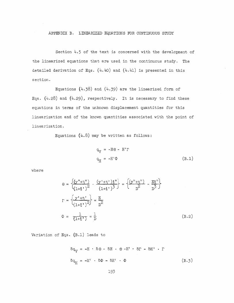
APPENDIX B. LINEARIZED EQUATIONS FOR CONTINUOUS STUDY
Section 4.5 of the text is concerned with the development of
the linearized e~uations that are used in the continuous study. The
detailed derivation of E~s. (4.40) and (4.41) is presented in this
section.
E~uations (4.38) and (4.39) are the linearized form of
E~s. (4.28) and (4.29), respectively. It is necessary to find these
equations in terms of the unknown displacement quantities for this
linearization and of the known ~uantities associated with the point of
linearization.
E~uations (4.8) may be written as follows:
-He - H'r
(B.l)
where
<P = (B.2)
Variation of Eqs. (B.l) leads to
oqv -H· 0 <9 - oH . <9 _HT • or - oH T • r
_Hi . o<P - oH' . <P
193
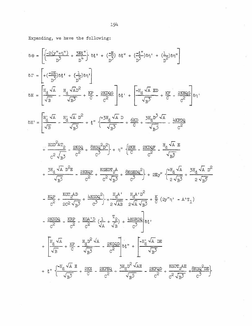
194
Expanding, we have the following:
+ KGD2AT2 _ 2KGQ + 8KGQ2Dj- + 1)" {2KE. _ 2KllQF _ Hd..fA E
C2 J;; C2
C3
C C2 .JB~
3Hd "l1: D2E 2KEQP KGEDT:! 8KGEDQ2l fI f-Hd .fA 3Hd "/A D2
+ :;5 - C2 + C2~B3 + c3 J+ 2Ey T2 .J;3+ 2,.JB?
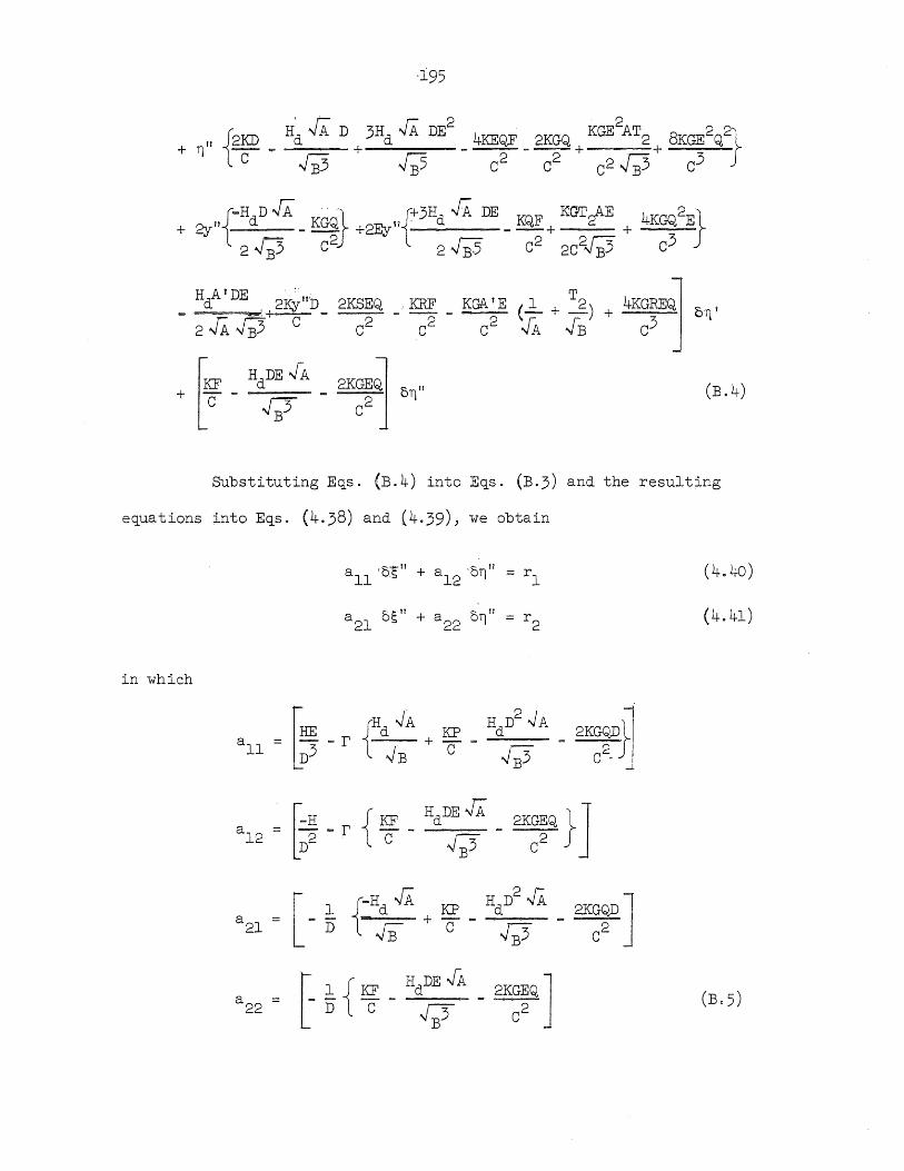
·195
+ '11" {2KD _ H~ JA. D + 3Hd .fA DE2 _ 4KEQF _ 2KGQ + KGE
2AT2 + 8KGE2Q2}
C JP5 J;5 C2
C2
C2 J;3 C3
{ .... HdD,fA .. ~. {7"3H
d ~ DE KJQF KiGT~E 4KGQ2E} + 2y" _ KGQ +2EyVi __ + + __ ____
2 J;) C2
2 ~ B5 C2 2C2.f;3 C3
Hi' 'DE _:+ 2~";D _ 2KSEQ ,KRF KGA 'E (1:... + T2) + 4KGruxJ OI]'
2 JA .JB3 C C2 - C2 - C2 '.fA.fB C3 J
+ t~ - 2KGE~ 0 II 2 '11 C
(B.4)
Substituting Eqs. (B.4) into Eqs. (B.3) and the resulting
equations into Eqs. (4.38) and (4.39)) we obtain
a '01" + a ·0'1'1" 11' 12 'I = r l
a 6; 11 + a on" r 21 22 'I = 2 (4.41)
in which
[- ~ fHd.fA -'- KP _ HdD2 .fA - 2KGQD ] a
21 = JB ' C J;5 C
2
t~{~-HdDE .fA
- 2KGEQ J (Bo 5) a22
= q C2
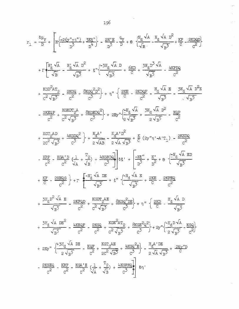
+ 3Hd .fA DE2 _ 4KEQF _ 2KGQ + KGE
2AT2 + 8KGE2Q.2}+ 2y,,{-HdD .fA _ KGQL
J;5 C2
C2
C2 .J B3 C3 2 J;3 CiJ
{:t3H
d ~A DE KQF KGT2AE 4KGQ~}' H~! DE2 liD + 2Ey11 ~ - - + + - + ~
2.JB5 C2
2C2 JB5 C3 2~~ C
2KSEQ. KRF KG/\. 'E (..l. + T2) + 4KGREQ11
1
OT)!
C 2 - C2 - C 2 :".fA.JB c3 1
197
When the above relations are substituted into Eqso (4040) and
(4.41)) the resulting expressions are linear in all displacement
quantities corresponding to this linearization. The coefficients of
these displacement quantities are expressed in terms of known quantities
evaluated at the point of linearization or quantities corresponding to
the dead load configuration.