Qualitative and Quantitative Analysis of a Bio-PEPAModel of the Gp130/JAK/STAT Signalling Pathway

Maria Luisa Guerriero

Laboratory for Foundations of Computer Science, The University of Edinburgh, UK

Abstract. Computational modelling of complex biochemical systems has grownin importance over recent years as a tool for supporting biological studies. Con-sequently, several formal languages have been recently proposed as modellinglanguages for biology. Among these, process algebras have been proved capableof providing researchers with new hypotheses on the behaviour of biochemicalsystems.Bio-PEPA is a process algebra recently defined for the modelling and analysisof biochemical systems, which provides modellers with a wide range of analysistechniques: models can be analysed by stochastic simulation, model-checking,and mathematical methods based on ordinary differential equations.In this work, we use Bio-PEPA for modelling the gp130/JAK/STAT signallingpathway, and we use both stochastic simulation and model-checking to analyseseveral qualitative and quantitative aspects of the system.

1 Introduction

Several modelling approaches have been used over recent years to analyse complexbiological systems such as signaling pathways, ranging from traditional mathematicalmethods based on differential equations to computational methods based on stochasticsimulation and model-checking. Each of these techniques can be more suitable thanothers in some context or to study some particular features of biological systems.

Process algebras are formal languages traditionally used to model distributed sys-tems of concurrent computing devices. Starting from the biochemical π-calculus [1],several other process algebras have been recently adapted in order to model biochemi-cal systems [2–5], following the “molecules as processes” paradigm introduced in thelandmark paper [6]: molecules are modelled as concurrent processes, and biochemicalreactions are represented by actions performed by synchronising processes.

Bio-PEPA [7, 8] is a process algebra specifically defined to model and analyse bio-chemical networks. Compared to other process algebras, Bio-PEPA uses a more ab-stract view of biochemical systems, the so-called “species as processes” abstraction:processes represent molecular species instead of single molecules, and multi-way syn-chronisations of processes represent changes in the amounts of molecular species re-sulting from biochemical reactions. Such an abstract view enables modellers to dealwith analysis techniques which are computationally infeasible when considering the“molecules as processes” abstraction.

The main feature of Bio-PEPA is that it integrates several kinds of analysis tech-niques. Both discrete stochastic and continuous deterministic models can be automati-cally generated from Bio-PEPA models, thus allowing modellers to perform time-series

analysis via stochastic simulation, Markovian analysis and ordinary differential equa-tions (ODEs); in addition, system properties can be verified through model-checkingand mathematical techniques such as bifurcation, stability and continuation analysis.Moreover, as for the other process algebras, Bio-PEPA is equipped with an operationalsemantics which supports various kinds of formal analysis (e.g. causality, equivalence,and reachability analysis).

In this work, we define a Bio-PEPA model of the gp130/JAK/STAT signalling path-way, a well-studied system which plays a major role in several biological processesboth in human and other organisms. A lot of experimental data is available about themolecules in the pathway, and some mathematical and computational models have beenalready developed. For these reasons, the gp130/JAK/STAT pathway represents a goodcase study for exploiting some of the possible Bio-PEPA analysis methods in order tostudy different aspects (both qualitative and quantitative) of the system, and comparethem with existing models.

The rest of the paper is structured as follows. First, the Bio-PEPA language is in-troduced in Sec. 2, while the pathway and the Bio-PEPA model are described in Sec. 3and Sec. 4, respectively. The following three sections are devoted to the analysis ofthe model: in Sec. 5 several qualitative properties are analysed via model-checking, inSec. 6 we present some stochastic simulation results, and in Sec. 7 model-checking isemployed for quantitative analysis. Finally, Sec. 8 is an overview of the related workand Sec. 9 contains some concluding remarks.

2 Bio-PEPA

Bio-PEPA [7, 8] is a process algebra which has been recently defined for the modellingand analysis of biochemical networks. It is a biologically-inspired language based onPEPA [9] and, differently from PEPA and other process algebras, it is able to explicitlyrepresent details such as stoichiometric coefficients and the roles of species in reactions,and it supports the definition of general kinetic laws. Bio-PEPA models can be analysedby different techniques (stochastic simulation, analysis based on ODEs, numerical solu-tion of the continuous-time Markov chain (CTMC), and probabilistic model-checking),since the mappings of Bio-PEPA models into specifications for those approaches havebeen defined [10].

The Bio-PEPA language is based on discrete levels of parameterised species: eachcomponent represents a species and its parameter may be interpreted as the number ofmolecules or discrete levels of concentration depending on the type of analysis to beapplied. Parametric levels are considered for the definition of the transition system andfor the derivation of a CTMC whose states represent the concentration levels of thespecies.

The syntax of Bio-PEPA is defined as:

S ::= (α, κ) op S | S + S | C P ::= P BCI

P | S (x)

where op = ↓ | ↑ | ⊕ | | �.The component S is called a species component and abstracts a molecular species,

whereas the component P, called a model component, describes the system and the in-teractions among components. The prefix term (α, κ) op S contains information about

the role of the species in the reaction associated with the action type α: κ is the stoichio-metric coefficient of the species and the prefix combinator “op” represents its role in thereaction. Specifically, ↓ indicates a reactant, ↑ a product, ⊕ an activator, an inhibitorand � a generic modifier. The operator “+” expresses the choice between possible ac-tions and the constant C is defined by an equation C

def= S . The parameter x ∈ IR+ in

S (x) represents the concentration of S . Finally, the process P BCI

Q denotes the cooper-ation between components: the set I determines those activities on which the operandsare forced to synchronise. Reaction rates are defined as functional rates associated withactions.

Bio-PEPA supports a modelling style in terms of concentration levels: the speciesamounts are discretised into a number of levels, from level 0 (i.e. species not present)to a maximum level N (which depends on the maximum concentration of the species).Each level represents an interval of concentration and the granularity of the system isexpressed in terms of the step size H (i.e. the length of the concentration interval).

Definition 1. A Bio-PEPA system P is a 6-tuple 〈V,N ,K ,FR,Comp, P〉, where:V isthe set of compartments,N is the set of quantities describing the species (i.e. H and N),K is the set of parameter definitions, FR is the set of functional rates, Components isthe set of definitions of species components, P is the model component describing thesystem.

For discrete state space analysis the behaviour of the system is defined in terms of anoperational semantics. A Stochastic Labelled Transition System (SLTS) is defined for aBio-PEPA system. From this we can obtain a Continuous Time Markov Chain (CTMC).Both the SLTS and the CTMC derived from Bio-PEPA are defined in terms of levels ofconcentration, and the generated Markov chain is called CTMC with levels. For a fulldescription of the language semantics see [10].

The Bio-PEPA language is supported by software tools such as the Bio-PEPA Work-bench [11], which automatically processes Bio-PEPA models and generates other rep-resentations in forms suitable for simulation and model-checking. For instance, the gen-erated simulation model can be executed using the Dizzy stochastic simulator [12]. Therepresentation which is used for discrete state space generation and analysis by numer-ical solution of the underlying CTMC is expressed in the reactive modules languagesupported by the PRISM model-checker [13]. In addition, the Bio-PEPA Workbenchgenerates reward structures and common CSL [14] formulae used in model-checking.

3 The Gp130/JAK/STAT Signalling Pathway

The gp130/JAK/STAT signalling pathway is a well-studied biological system, of greatclinical interest because of its key role in human fertility, neuronal repair and haemato-logical development [15–17]. Much experimental data is available on this pathway, anda few mathematical and computational models [18–21] have been developed.

The signalling cascade in the gp130/JAK/STAT pathway is triggered by membersof the family of IL (interleukin)-6-type cytokines binding to plasma membrane receptorcomplexes containing the common signal transducing receptor chain gp130 (glycopro-tein 130). Among the targets of gp130 signal transduction, we consider the transcription

factors of the STAT (signal transducers and activators of transcription) family, in partic-ular STAT3. A key feature of the pathway is the nuclear/cytoplasmic shuttling of STATs:upon activation, STATs can translocate into the nucleus and activate the transcription ofdownstream gene targets.

Different cytokines signal through the formation of different receptor complexes,all of them containing gp130 and another subunit. We focus here on two differentcytokines: LIF (leukaemia inhibitory factor) and OSM (oncostatin M). LIF signalsthrough an heterodimeric receptor complex gp130:LIFR. OSM exhibits the uncommonability to signal through two different receptor complexes: the type I OSM receptorcomplex (gp130:LIFR), and the type II OSM receptor complex (gp130:OSMR).

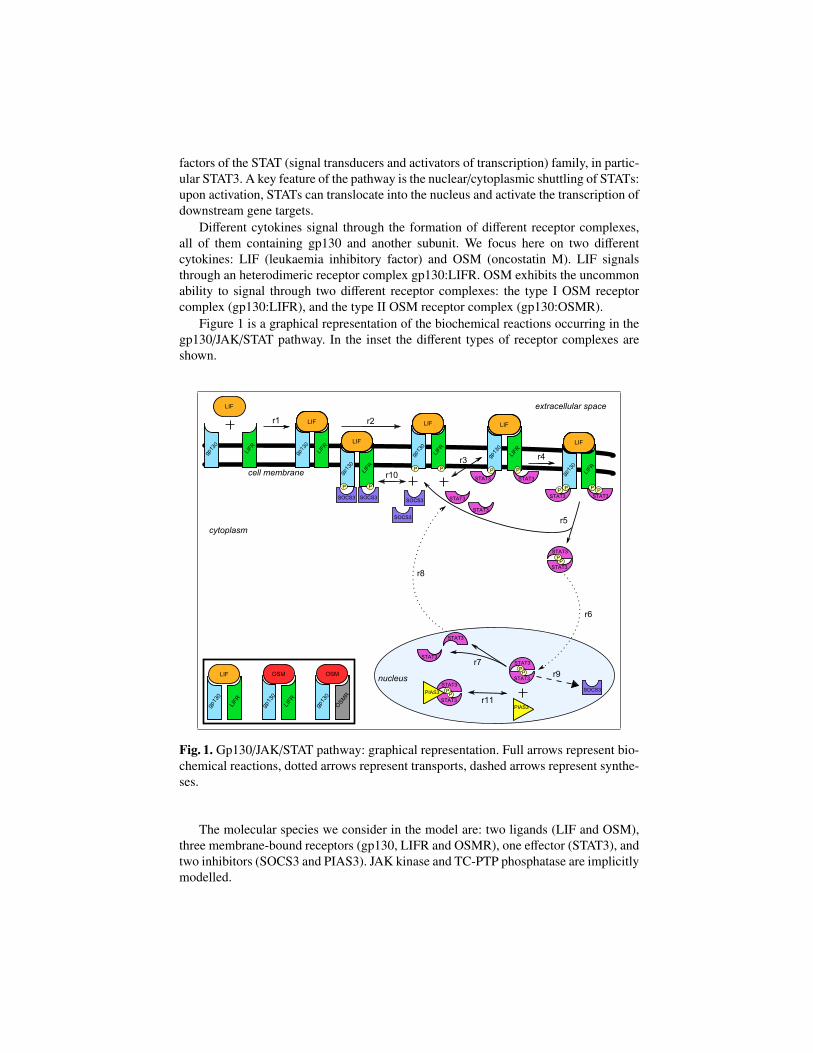
Figure 1 is a graphical representation of the biochemical reactions occurring in thegp130/JAK/STAT pathway. In the inset the different types of receptor complexes areshown.

Fig. 1. Gp130/JAK/STAT pathway: graphical representation. Full arrows represent bio-chemical reactions, dotted arrows represent transports, dashed arrows represent synthe-ses.

The molecular species we consider in the model are: two ligands (LIF and OSM),three membrane-bound receptors (gp130, LIFR and OSMR), one effector (STAT3), andtwo inhibitors (SOCS3 and PIAS3). JAK kinase and TC-PTP phosphatase are implicitlymodelled.

Four compartments are involved in the system: the exosol (the extracellular space,where the two ligands are located), the cell membrane (location of the receptors), thecytosol (initial location of STAT3), and the nucleus (in which STAT3 can translocate).

Receptors are activated by ligand bindings, and active receptors dimerise to formreceptor complexes (gp130:LIFR or gp130:OSMR) (reaction r1 in Fig. 1). Once thereceptor dimeric complex is formed, each receptor subunit (gp130, LIFR and OSMR)can undergo JAK-mediated phosphorylation (r2). STAT3 can bind on receptors’ phos-phorylated sites (r3), and the binding of STAT3 leads to its activation (phosphorylation)(r4).

Once phosphorylated, STAT3 dissociates from the receptor complex, and its phos-phorylated site allows STAT3 to homodimerise (r5). When STAT3 is in dimeric form,it can translocate into the nucleus (r6) where it can carry out its specific functions (notmodelled here): STAT3 binds to the DNA, thus activating the transcription of down-stream gene targets. Nuclear STAT3 dimers are inactivated through TC-PTP -mediateddephosphorylation, which leads to the dimers’ dissociation (r7) and to STAT3 export tothe cytoplasm (r8), where STAT3 can undergo additional cycles of activation.

The two inhibition mechanisms considered are due to SOCS3 and PIAS3. SOCS3 issynthesised by STAT3 (r9) and it acts by competing with STAT3 in binding to receptors(r10). PIAS3 acts by binding to active nuclear STAT3 (r11).

4 The Bio-PEPA Model

A Bio-PEPA model of the gp130/JAK/STAT pathway has been developed. The fullmodel can be downloaded from [22]. The model and the reaction rates are based on [21],though some differences are present due to the conceptual differences in the used mod-elling languages (see Sec. 8 for a discussion of such differences). All kinetic laws areassumed to be mass-action (i.e. depending on the amount of reactants and on givenkinetic constants).

Each possible form of the molecular species is modelled as a distinct Bio-PEPAspecies component. For instance, STAT3 is modelled by four distinct species compo-nents representing, respectively, the cytoplasmic dephosphorylated monomeric form(STAT3 c), the cytoplasmic phosphorylated dimeric form (STAT3-PD c), the nuclearphosphorylated dimeric form (STAT3-PD n), and the nuclear dephosphorylated mono-meric form (STAT3 n); further species components are defined for each state of eachcomplex containing STAT3.

Reactions and biochemical modifications are represented by reactions over whichthe involved species components synchronise. For instance, the reaction representing r7in Fig. 1 is modelled as the reaction dephospho dedimer stat59, which decreases theamount of STAT3-PD n and increases (with stoichiometry coefficient 2) the amount ofSTAT3 n.

As an example, the definitions of the species STAT3-PD n and STAT3 n are reported(here we use the simplified syntax of the Bio-PEPA Workbench, in which the trailing Sin prefix terms (α, κ) op S can be omitted).

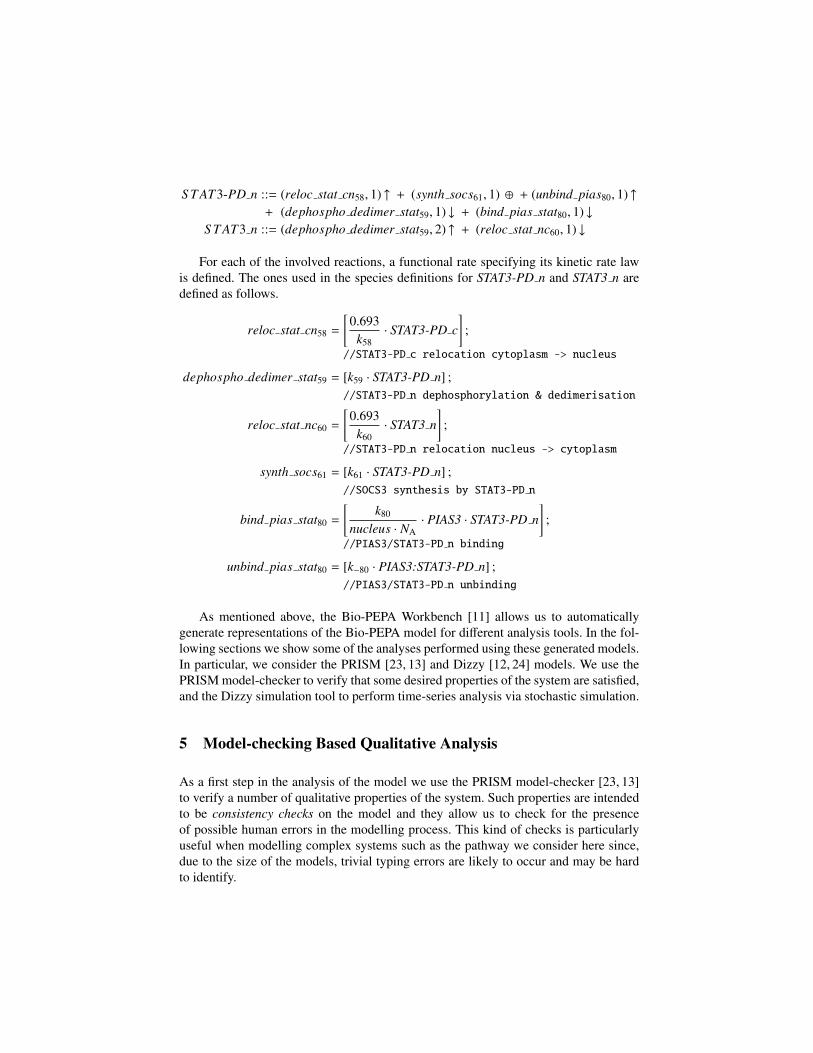
S T AT3-PD n ::= (reloc stat cn58, 1) ↑ + (synth socs61, 1) ⊕ + (unbind pias80, 1) ↑+ (dephospho dedimer stat59, 1) ↓ + (bind pias stat80, 1) ↓

S T AT3 n ::= (dephospho dedimer stat59, 2) ↑ + (reloc stat nc60, 1) ↓

For each of the involved reactions, a functional rate specifying its kinetic rate lawis defined. The ones used in the species definitions for STAT3-PD n and STAT3 n aredefined as follows.

reloc stat cn58 =

[0.693

k58· STAT3-PD c

];

//STAT3-PD c relocation cytoplasm -> nucleus

dephospho dedimer stat59 = [k59 · STAT3-PD n] ;//STAT3-PD n dephosphorylation & dedimerisation

reloc stat nc60 =

[0.693

k60· STAT3 n

];

//STAT3-PD n relocation nucleus -> cytoplasm

synth socs61 = [k61 · STAT3-PD n] ;//SOCS3 synthesis by STAT3-PD n

bind pias stat80 =

[k80

nucleus · NA· PIAS3 · STAT3-PD n

];

//PIAS3/STAT3-PD n binding

unbind pias stat80 = [k−80 · PIAS3:STAT3-PD n] ;//PIAS3/STAT3-PD n unbinding

As mentioned above, the Bio-PEPA Workbench [11] allows us to automaticallygenerate representations of the Bio-PEPA model for different analysis tools. In the fol-lowing sections we show some of the analyses performed using these generated models.In particular, we consider the PRISM [23, 13] and Dizzy [12, 24] models. We use thePRISM model-checker to verify that some desired properties of the system are satisfied,and the Dizzy simulation tool to perform time-series analysis via stochastic simulation.

5 Model-checking Based Qualitative Analysis

As a first step in the analysis of the model we use the PRISM model-checker [23, 13]to verify a number of qualitative properties of the system. Such properties are intendedto be consistency checks on the model and they allow us to check for the presenceof possible human errors in the modelling process. This kind of checks is particularlyuseful when modelling complex systems such as the pathway we consider here since,due to the size of the models, trivial typing errors are likely to occur and may be hardto identify.

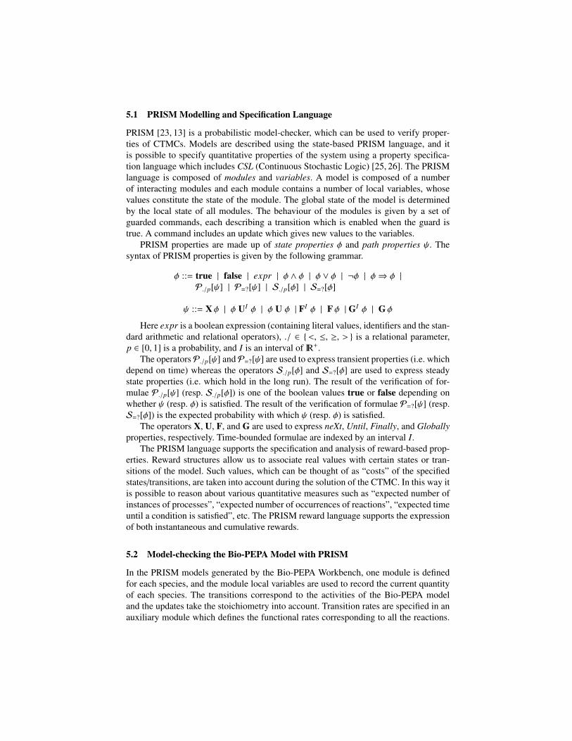
5.1 PRISM Modelling and Specification Language

PRISM [23, 13] is a probabilistic model-checker, which can be used to verify proper-ties of CTMCs. Models are described using the state-based PRISM language, and itis possible to specify quantitative properties of the system using a property specifica-tion language which includes CSL (Continuous Stochastic Logic) [25, 26]. The PRISMlanguage is composed of modules and variables. A model is composed of a numberof interacting modules and each module contains a number of local variables, whosevalues constitute the state of the module. The global state of the model is determinedby the local state of all modules. The behaviour of the modules is given by a set ofguarded commands, each describing a transition which is enabled when the guard istrue. A command includes an update which gives new values to the variables.

PRISM properties are made up of state properties φ and path properties ψ. Thesyntax of PRISM properties is given by the following grammar.

φ ::= true | false | expr | φ ∧ φ | φ ∨ φ | ¬φ | φ⇒ φ |P./p[ψ] | P=?[ψ] | S./p[φ] | S=?[φ]

ψ ::= X φ | φ UI φ | φ U φ | FI φ | F φ | GI φ | G φ

Here expr is a boolean expression (containing literal values, identifiers and the stan-dard arithmetic and relational operators), ./ ∈ {<, ≤, ≥, > } is a relational parameter,p ∈ [0, 1] is a probability, and I is an interval of IR+.

The operatorsP./p[ψ] andP=?[ψ] are used to express transient properties (i.e. whichdepend on time) whereas the operators S./p[φ] and S=?[φ] are used to express steadystate properties (i.e. which hold in the long run). The result of the verification of for-mulae P./p[ψ] (resp. S./p[φ]) is one of the boolean values true or false depending onwhether ψ (resp. φ) is satisfied. The result of the verification of formulae P=?[ψ] (resp.S=?[φ]) is the expected probability with which ψ (resp. φ) is satisfied.

The operators X, U, F, and G are used to express neXt, Until, Finally, and Globallyproperties, respectively. Time-bounded formulae are indexed by an interval I.

The PRISM language supports the specification and analysis of reward-based prop-erties. Reward structures allow us to associate real values with certain states or tran-sitions of the model. Such values, which can be thought of as “costs” of the specifiedstates/transitions, are taken into account during the solution of the CTMC. In this way itis possible to reason about various quantitative measures such as “expected number ofinstances of processes”, “expected number of occurrences of reactions”, “expected timeuntil a condition is satisfied”, etc. The PRISM reward language supports the expressionof both instantaneous and cumulative rewards.

5.2 Model-checking the Bio-PEPA Model with PRISM

In the PRISM models generated by the Bio-PEPA Workbench, one module is definedfor each species, and the module local variables are used to record the current quantityof each species. The transitions correspond to the activities of the Bio-PEPA modeland the updates take the stoichiometry into account. Transition rates are specified in anauxiliary module which defines the functional rates corresponding to all the reactions.

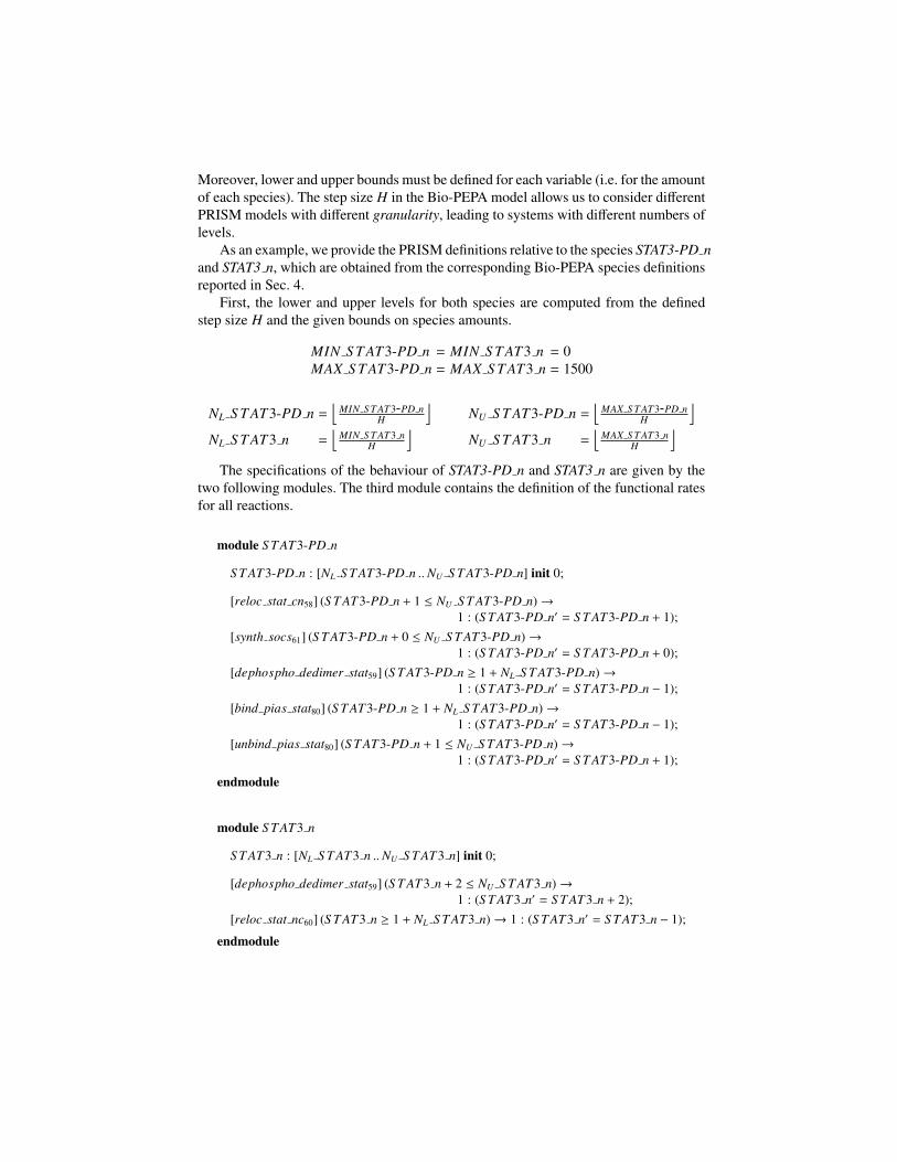
Moreover, lower and upper bounds must be defined for each variable (i.e. for the amountof each species). The step size H in the Bio-PEPA model allows us to consider differentPRISM models with different granularity, leading to systems with different numbers oflevels.

As an example, we provide the PRISM definitions relative to the species STAT3-PD nand STAT3 n, which are obtained from the corresponding Bio-PEPA species definitionsreported in Sec. 4.

First, the lower and upper levels for both species are computed from the definedstep size H and the given bounds on species amounts.

MIN S T AT3-PD n = MIN S T AT3 n = 0MAX S T AT3-PD n = MAX S T AT3 n = 1500

NL S T AT3-PD n =⌊

MIN S T AT3-PD nH

⌋NU S T AT3-PD n =

⌊MAX S T AT3-PD n

H

⌋NL S T AT3 n =

⌊MIN S T AT3 n

H

⌋NU S T AT3 n =

⌊MAX S T AT3 n

H

⌋The specifications of the behaviour of STAT3-PD n and STAT3 n are given by the

two following modules. The third module contains the definition of the functional ratesfor all reactions.

module S T AT3-PD n

S T AT3-PD n : [NL S T AT3-PD n ..NU S T AT3-PD n] init 0;

[reloc stat cn58] (S T AT3-PD n + 1 ≤ NU S T AT3-PD n)→1 : (S T AT3-PD n′ = S T AT3-PD n + 1);

[synth socs61] (S T AT3-PD n + 0 ≤ NU S T AT3-PD n)→1 : (S T AT3-PD n′ = S T AT3-PD n + 0);

[dephospho dedimer stat59] (S T AT3-PD n ≥ 1 + NL S T AT3-PD n)→1 : (S T AT3-PD n′ = S T AT3-PD n − 1);

[bind pias stat80] (S T AT3-PD n ≥ 1 + NL S T AT3-PD n)→1 : (S T AT3-PD n′ = S T AT3-PD n − 1);

[unbind pias stat80] (S T AT3-PD n + 1 ≤ NU S T AT3-PD n)→1 : (S T AT3-PD n′ = S T AT3-PD n + 1);

endmodule

module S T AT3 n

S T AT3 n : [NL S T AT3 n ..NU S T AT3 n] init 0;

[dephospho dedimer stat59] (S T AT3 n + 2 ≤ NU S T AT3 n)→1 : (S T AT3 n′ = S T AT3 n + 2);

[reloc stat nc60] (S T AT3 n ≥ 1 + NL S T AT3 n)→ 1 : (S T AT3 n′ = S T AT3 n − 1);

endmodule

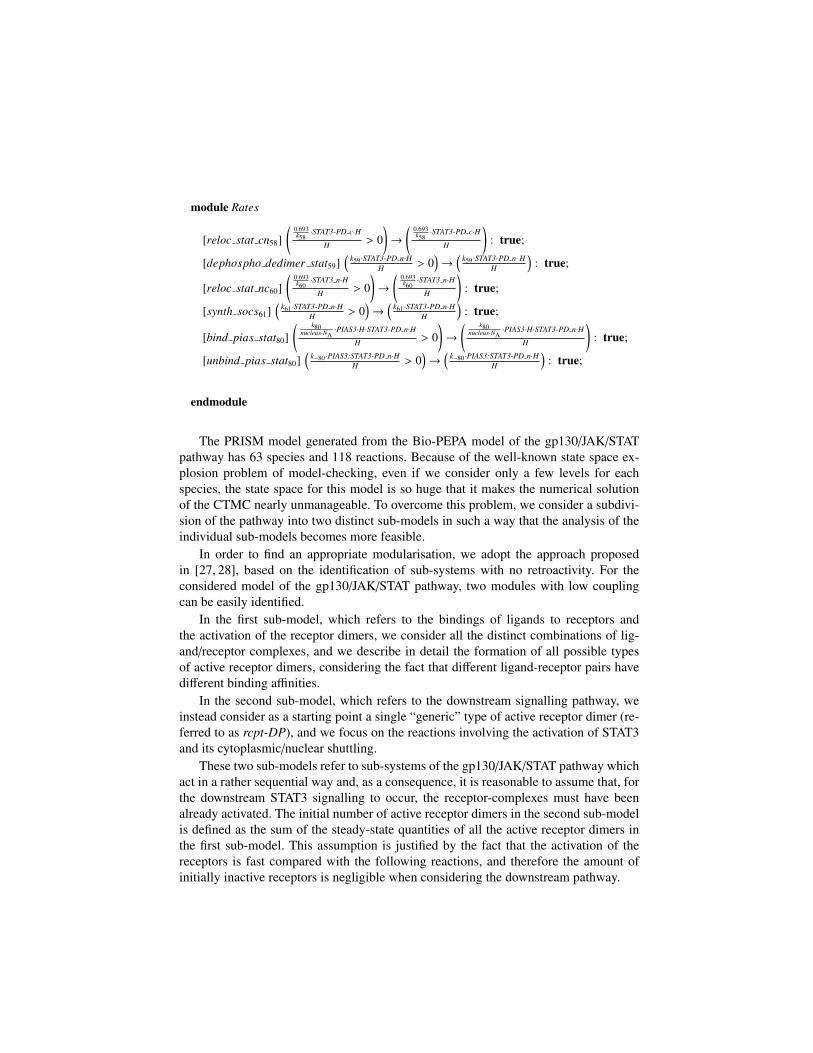
module Rates

[reloc stat cn58](

0.693k58·STAT3-PD c·H

H > 0)→

(0.693k58·STAT3-PD c·H

H

): true;

[dephospho dedimer stat59](

k59 ·STAT3-PD n·HH > 0

)→

(k59 ·STAT3-PD n·H

H

): true;

[reloc stat nc60](

0.693k60·STAT3 n·H

H > 0)→

(0.693k60·STAT3 n·H

H

): true;

[synth socs61](

k61 ·STAT3-PD n·HH > 0

)→

(k61 ·STAT3-PD n·H

H

): true;

[bind pias stat80]( k80

nucleus·NA·PIAS3·H·STAT3-PD n·H

H > 0)→

( k80nucleus·NA

·PIAS3·H·STAT3-PD n·H

H

): true;

[unbind pias stat80](

k−80 ·PIAS3:STAT3-PD n·HH > 0

)→

(k−80 ·PIAS3:STAT3-PD n·H

H

): true;

endmodule

The PRISM model generated from the Bio-PEPA model of the gp130/JAK/STATpathway has 63 species and 118 reactions. Because of the well-known state space ex-plosion problem of model-checking, even if we consider only a few levels for eachspecies, the state space for this model is so huge that it makes the numerical solutionof the CTMC nearly unmanageable. To overcome this problem, we consider a subdivi-sion of the pathway into two distinct sub-models in such a way that the analysis of theindividual sub-models becomes more feasible.

In order to find an appropriate modularisation, we adopt the approach proposedin [27, 28], based on the identification of sub-systems with no retroactivity. For theconsidered model of the gp130/JAK/STAT pathway, two modules with low couplingcan be easily identified.

In the first sub-model, which refers to the bindings of ligands to receptors andthe activation of the receptor dimers, we consider all the distinct combinations of lig-and/receptor complexes, and we describe in detail the formation of all possible typesof active receptor dimers, considering the fact that different ligand-receptor pairs havedifferent binding affinities.

In the second sub-model, which refers to the downstream signalling pathway, weinstead consider as a starting point a single “generic” type of active receptor dimer (re-ferred to as rcpt-DP), and we focus on the reactions involving the activation of STAT3and its cytoplasmic/nuclear shuttling.

These two sub-models refer to sub-systems of the gp130/JAK/STAT pathway whichact in a rather sequential way and, as a consequence, it is reasonable to assume that, forthe downstream STAT3 signalling to occur, the receptor-complexes must have beenalready activated. The initial number of active receptor dimers in the second sub-modelis defined as the sum of the steady-state quantities of all the active receptor dimers inthe first sub-model. This assumption is justified by the fact that the activation of thereceptors is fast compared with the following reactions, and therefore the amount ofinitially inactive receptors is negligible when considering the downstream pathway.

As discussed in [27, 28], the absence of retroactivity ensures that the modularisa-tion has no significant effect on the overall behaviour of the system. This, together withthe fact that we use the output of the first sub-model as input of the second sub-model,ensures that the structural qualitative properties verified for the individual sub-modelsin the rest of this section also hold for the full model. Particular care should be takenwhen verifying quantitative temporal properties over sub-models. Here we only con-sider semi-quantitative analysis (Sec. 7) as we are interested in relative rather than ab-solute values. Therefore, in this particular case, the absence of retroactivity ensures thevalidity, in the full model, of the analysis results obtained in the sub-models. In general,however, the actual reaction rates in the composite model (and therefore the analysisresults) might be different from the ones in the sub-models, and more advanced ap-proaches for modularisation should be applied.

In the rest of this section we use H = 200 as the step size for the ligands-receptorssub-model, and H = 300 for the downstream sub-model. See Sec. 7 for a discussion ofthe choice of step size values.

Deadlock Detection. Deadlock states are the ones in which no transition is enabled.In some cases the presence of deadlock states is (correctly) due to the presence of ir-reversible reactions which lead to the transformation of all reactants into non-reactiveproteins. In other cases deadlocks could be due to the scarcity of one of the reactants ofa multimolecular reaction; in our model, for instance, all receptors are consumed (i.e.transformed into different forms, such as dimers) while still ligands are available. Inother cases deadlocks could be caused by modelling errors.

PRISM automatically detects deadlock states when building the state space of mod-els, and this feature can be considered the first step in the identification of potentialmodelling errors.

For instance, in the ligands-receptors sub-model, any state in which ligands arepresent while all gp130 receptors have been consumed is a deadlock. This suggests thatgp130 is the bottleneck of the system.

Species Invariants. One simple and yet interesting property that can be verified is thepresence of invariants in the amount of the involved proteins.

Species invariants are commonly present in biochemical systems because of theexistence of basic constraints such as the law of conservation of mass, which states thatthe amount (i.e. mass) of reactants consumed by a reaction must be equal to the amountof products of the reaction.

For instance, given the conservation of mass and the absence of synthesis and degra-dation reactions, we expect that the sum of the amounts of LIFR receptor present in itsvarious possible forms (free, as gp130:LIF:LIFR complex and as gp130:OSM:LIFRcomplex, with one or both of its subunits phosphorylated) is constant (and equal to theLIFR initial amount).

The satisfaction of the following properties confirms the existence of the expectedinvariants on the total amount of ligands and receptors (as an example, we report theones for LIF and LIFR).

P≥1[G (LIF + gp130:LIF:LIFR + gp130-P:LIF:LIFR + gp130:LIF:LIFR-P +

gp130-P:LIF:LIFR-P = NU LIF)] → true

P≥1[G (LIFR + gp130:LIF:LIFR + gp130:OSM:LIFR + gp130-P:LIF:LIFR +

gp130:LIF:LIFR-P + gp130-P:LIF:LIFR-P + gp130-P:OSM:LIFR +

gp130:OSM:LIFR-P + gp130-P:OSM:LIFR-P = NU LIFR)] → true

Here, and in the rest of the section, the notation P./p[ψ]→ true (resp. false) meansthat ψ is satisfied (resp. is not satisfied), while the notation P=?[ψ] → p (with p ∈ IR)means that the result of ψ is the probability p.

Reachability Analysis. Reachability properties allow us to verify whether a given stateis eventually reached. States of interest can be, for instance, the ones in which somespecies reaches a threshold or is totally consumed, or when the amounts of two speciescoincide.

We consider here the states in which a certain number of receptors are phosphory-lated, and the ones in which a certain amount of active nuclear STAT3 (STAT3-PD n)is present.

We consider first the ligands-receptors sub-model. The satisfaction of the first ofthe following properties guarantees that a state in which one fourth of the total amountof available receptors is phosphorylated is always reached at some time point. On thecontrary, the second property, which is not satisfied, proves that we do not necessarilyreach a state with one third of receptors phosphorylated.

P≥1[F (gp130-P:LIF:LIFR-P + gp130-P:OSM:LIFR-P + gp130-P:OSM:OSMR-P >

(NU OS MR + NU LIFR + NU gp130) / 4)] → true

P≥1[F (gp130-P:LIF:LIFR-P + gp130-P:OSM:LIFR-P + gp130-P:OSM:OSMR-P >

(NU OS MR + NU LIFR + NU gp130) / 3)] → false

The next property, instead, guarantees that in general we could reach a system whereno gp130:OSMR receptor complex is activated.

P≥1[F (gp130-P:OSM:OSMR-P > 0)] → false

Regarding the downstream sub-model, we check for the following properties, whichguarantee that, at some time point, at least half the initial amount of STAT3 has beentransported into the nucleus and activated, but not all of it.

P≥1[F (S T AT3-PD n > NU S T AT3 c / 2)] → true

P≥1[F (S T AT3-PD n > NU S T AT3 c)] → false

Reversibility. A system is called reversible if the initial state is reachable from anyother state (i.e. the system is able to self-reinitialise). More generally, a state is calledreversible if it can be reached again at some later time point.

The following property, if satisfied, guarantees the reversibility of the system: itstates that it is always possible to return to the initial state (in the PRISM language“init” is a predefined formula which completely specifies the initial state).

P=?[G (“init”⇒ P≥1[X (!“init”⇒ P≥1[F (“init”)])])]

For the ligands-receptors sub-system the result of this property is 0, since we haveconsidered bindings to be irreversible and, therefore, the system cannot return to theinitial state in which all receptors and ligands are free.

The downstream sub-system, instead, is reversible (the result of the property is 1),thanks to the cytoplasmic/nuclear STAT3 shuttling, which enables the system to returnto the initial state in which cytoplasmic STAT3 molecules are not phosphorylated andnot bound to receptor dimers.

Liveness. The notion of liveness of a reaction in a given state refers to the possibilityof it occurring in such a state. In particular, it is interesting to know which reactions arelive in the initial state.

Since PRISM properties are state-based, it is not possible to explicitly check forthe occurrence of a given reaction. However, knowing how each model component isaffected by the occurrence of a given reaction, we can verify this kind of property bychecking for the expected variations in the involved components.

We are interested, for instance, in verifying that in the initial state the binding re-actions between ligands and receptors can occur, leading to the three possible types ofligand/receptor dimers (gp130:LIF:LIFR, gp130:OSM:LIFR, and gp130:OSM:OSMR).

The following three properties are satisfied, confirming that the three known typesof complexes can be formed.

P≥1[G (“init”⇒ P>0[X (gp130 = NU gp130 − 1 & LIF = NU LIF − 1 &LIFR = NU LIFR − 1)])] → true

P≥1[G (“init”⇒ P>0[X (gp130 = NU gp130 − 1 & OS M = NU OS M − 1 &LIFR = NU LIFR − 1)])] → true

P≥1[G (“init”⇒ P>0[X (gp130 = NU gp130 − 1 & OS M = NU OS M − 1 &OS MR = NU OS MR − 1)])] → true

The following property, instead, is not satisfied: it states, as desired, that LIF cannotbind to receptors to form gp130:OSMR dimers.

P≥1[G (“init”⇒ P>0[X (gp130 = NU gp130 − 1 & LIF = NU LIF − 1 &OS MR = NU OS MR − 1)])] → false

Causality Analysis. Causality relations between given reactions can be expressed andverified by properties which relate the order of “appearance” of relevant molecules.This kind of property can be used, for instance, to verify the order in which intermediateproducts are formed within a cascade of events.

A form of causality relation can be expressed by using the sequence and conse-quence relations defined in [29]: specifically, while sequence formulae describe order-ing relations between events (e.g. “in order to reach a given state, we must first reachanother one”), consequence formulae describe causal relations (e.g. “if a given stateoccurs, it is necessarily followed by a second one”).

For example, the ordering and causality relations between STAT3 phosphorylation,homodimerisation and relocation into the nucleus can be verified by the following pairsof properties (assuming at system initialisation all STAT3 is present in cytoplasmicmonomeric form (STAT3-P c).

When the result of the first property is 0, such a property states that it is not pos-sible for a STAT3-PD c molecule to be present if in all previous states we had norcpt-DP:STAT3-DP1 (a complex formed by a receptor dimer and a STAT3 molecule).Similarly, the following property (when it evaluates to 0) states that STAT3-PD c mustbe produced before STAT3-PD n appears.

P=?[(rcpt-DP:STAT3-DP1 = 0) U S T AT3-PD c > 0]→ 0

P=?[(S T AT3-PD c = 0) U S T AT3-PD n > 0]→ 0

The following two properties complement the previous two, stating that if at leastone complex rcpt-DP:STAT3-DP1 is formed, then at least one STAT3-PD c moleculewill necessarily be formed.

P=?[G (rcpt-DP:STAT3-DP1 > 0⇒ P≥1[F (S T AT3-PD c > 0)])]→ 1

P=?[G (S T AT3-PD c > 0⇒ P≥1[F (S T AT3-PD n > 0)])]→ 1

As another example, the following two properties verify that the transport of phos-phorylated STAT3 dimers can only occur from the cytoplasm to the nucleus, but notvice versa. The result of the first property is 0 (i.e. transport of STAT3-PD can occurfrom cytoplasm to nucleus), while the result of the second property is 1 (i.e. transportof STAT3-PD cannot occur from nucleus to cytoplasm) for all reachable values of i, j.

P=?[F (S T AT3-PD c = i & S T AT3-PD n = j &P≤0[X (S T AT3-PD c = i − 1 &S T AT3-PD n = j + 1)])] → 0

P=?[F (S T AT3-PD c = i & S T AT3-PD n = j &P≤0[X (S T AT3-PD c = i + 1 &S T AT3-PD n = j − 1)])] → 1

Conversely, the transport of dephosphorylated STAT3 monomers can only occurfrom the nucleus to the cytoplasm.

P=?[F (S T AT3 c = i & S T AT3 n = j &P≤0[X (S T AT3 c = i − 1 & S T AT3 n = j + 1)])] → 1

P=?[F (S T AT3 c = i & S T AT3 n = j &P≤0[X (S T AT3 c = i + 1 & S T AT3 n = j − 1)])] → 0

6 Simulation Based Time-series Analysis

In the previous section we have used model-checking in order to check for a number ofsimple formulae which guarantee us that some key properties of the gp130/JAK/STATmodel are satisfied. This analysis allows us to be more confident about the absence ofmodelling errors.

Now we progress our analysis of the model by means of stochastic simulation.We report here some results obtained by simulating the full model (comprising boththe ligands-receptors and the downstream sub-systems) using the Gibson-Bruck [30]stochastic simulation engine implemented in Dizzy [12, 24].

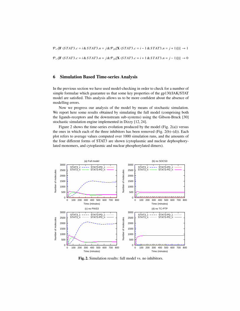
Figure 2 shows the time-series evolution produced by the model (Fig. 2(a)) versusthe ones in which each of the three inhibitors has been removed (Fig. 2(b)–(d)). Eachplot refers to average values computed over 1000 simulation runs, and the amounts ofthe four different forms of STAT3 are shown (cytoplasmic and nuclear dephosphory-lated monomers, and cytoplasmic and nuclear phosphorylated dimers).

0

500

1000

1500

2000

2500

3000

0 100 200 300 400 500 600 700 800

Num

ber

of m

olec

ules

Time (minutes)

(a) Full model

STAT3_cSTAT3_n

STAT3-PD_cSTAT3-PD_n

0

500

1000

1500

2000

2500

3000

0 100 200 300 400 500 600 700 800

Num

ber

of m

olec

ules

Time (minutes)

(b) no SOCS3

STAT3_cSTAT3_n

STAT3-PD_cSTAT3-PD_n

0

500

1000

1500

2000

2500

3000

0 100 200 300 400 500 600 700 800

Num

ber

of m

olec

ules

Time (minutes)

(c) no PIAS3

STAT3_cSTAT3_n

STAT3-PD_cSTAT3-PD_n

0

500

1000

1500

2000

2500

3000

0 100 200 300 400 500 600 700 800

Num

ber

of m

olec

ules

Time (minutes)

(d) no TC-PTP

STAT3_cSTAT3_n

STAT3-PD_cSTAT3-PD_n

Fig. 2. Simulation results: full model vs. no inhibitors.

In all the performed simulations, at system initialisation STAT3 is only presentin cytoplasmic monomeric form. As shown in Fig. 2(a), as time passes, STAT3 isphosphorylated, dimerised, and transported into the nucleus, until the systems reachesa state in which the inhibition of nuclear STAT3 by dephosphorylation and the nu-clear/cytoplasmic shuttling lead nuclear and cytoplasmic STAT3 to be in equilibrium.

When the amount of nuclear STAT3 increases significantly, the inhibitory role ofSOCS3 (which is under transcription control of STAT3) comes into play (Fig. 2(b)).SOCS3 is responsible for signal attenuation and, hence, after reaching a peak, nuclearSTAT3 decreases.

PIAS3 slows down the production of active nuclear STAT3 by binding to it (Fig. 2(c)).Therefore, if PIAS3 is present, part of nuclear STAT3 is bound to it, while, if PIAS3 isknocked down, the amount of available STAT3 increases.

A third inhibitor, TC-PTP, allows nuclear STAT3 to translocate back into the cyto-plasm, by dephosphorylating it (Fig. 2(d)). If TC-PTP is present, STAT3 nuclear/cyto-plasmic shuttling occurs; instead, if TC-PTP is knocked out (i.e. if nuclear STAT3 isnot dephosphorylated), STAT3 accumulates in the nucleus, whilst cytoplasmic STAT3molecules quickly disappear.

7 Semi-quantitative Analysis of the CTMC with Levels

In Sec. 5 we have shown how model-checking can be used in order to discover mod-elling errors by checking for some basic properties which guarantee the model to behaveas expected. In this section, instead, we use model-checking also for quantitative anal-ysis, with the purpose of completing the simulation-based analysis in order to provideadditional insight on the behaviour of the gp130/JAK/STAT pathway.

The main advantage of model-checking with respect to stochastic simulation is thefact that model-checking is exhaustive: it explores all the possible behaviours of themodel and it does not require us to compute an average behaviour of a number ofstochastic simulation runs.

As mentioned before, the main disadvantage of model-checking is the state spaceexplosion problem, which implies that we cannot deal with too many levels for themodel components without inducing an intractable model.

In has been shown (see [10]) that, as the number of levels increases, the behaviour ofthe CTMC with levels tends to the behaviour of ODEs (when the number of moleculesis large enough to average out the randomness of the system); this result guarantees thetheoretical correctness of the approach. However, if the number of levels is too small,the error introduced by the discretisation becomes significant and the numerical solutionof the generated CTMC fails to reproduce the correct behaviour.

The number of levels for model components is related to the step size H and tothe upper NU and lower NL bounds for each species. The step size H represents thegranularity of the system, and it directly affects the accuracy of the results; the upper andlower bounds are also relevant to the accuracy, since imposing bounds on the numbersof molecules causes a state space truncation which might potentially have impact on thebehaviour of the system.

Therefore, when performing CTMC analysis of Bio-PEPA models, the choice of thestep size and of the upper and lower bounds is essential: they must be carefully selectedso that the number of levels to be used for the model components is a suitable trade-off

between accuracy and efficiency.In the following sections we report some of the results obtained by using the PRISM

model-checker to perform quantitative analysis. First we consider reward-based prop-erties which allow us to observe the time-series for some of the species of the system(for comparison with the stochastic simulation), and we discuss the error introduced bydiscretising and bounding the model; afterwards, we define further properties in orderto compute additional (semi-)quantitative measures.

Time-series Analysis Using State Rewards. A reward structure is automatically de-fined by the Bio-PEPA Workbench for each PRISM component, and it can be referredto either by the component name or by an integer value (implicitly assigned to rewardstructures based on the order in which they are defined). These reward structures asso-ciate an instantaneous reward equal to the current amount of the corresponding molecu-lar species with each state. The evaluation of these reward-based properties correspondsto computing an average behaviour for the species at given time points.

As an example, the following reward is used to observe the time evolution of thereceptor dimer gp130:LIF:LIFR.

rewards “gp130:LIF:LIFR”true : gp130:LIF:LIFR · H;

endrewards

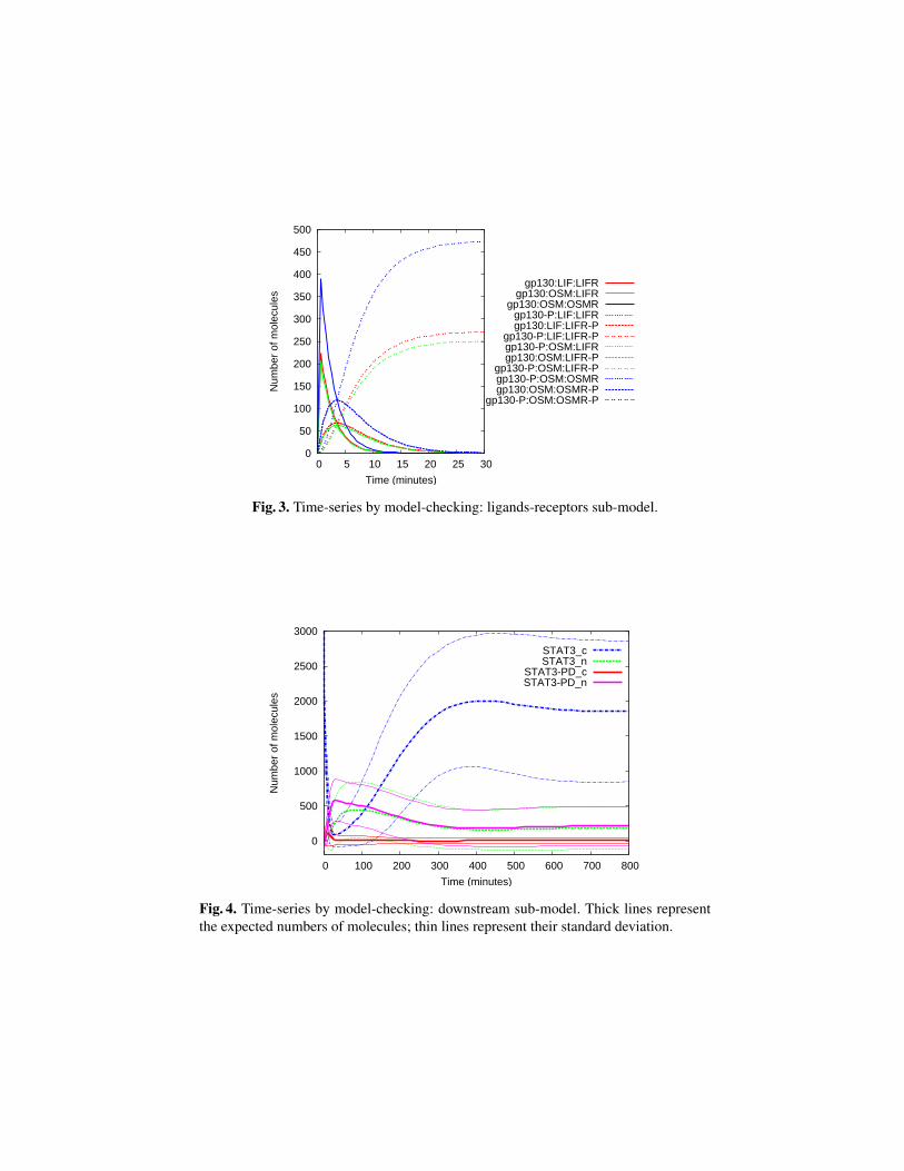
Figure 3 reports the results obtained by verifying on the ligands-receptors sub-system the reward-based property

Ri=?[I = T ]

for time points T ≤ 30 minutes, where i is an integer variable used to index the rewardstructure of interest.

Figure 4, instead, reports the results obtained by verifying the same reward-basedproperty for time points T ≤ 800 minutes on the downstream sub-system. In this figure,we also report the standard deviation of the number of molecules, which is computedby exploiting reward structures associating the square of the number of molecules ofeach species with each state: the standard deviation is calculated as the square root ofthe variance E(Y)2 − E(Y2), where Y is the random variable representing a species inthe network, whereas E(Y) and E(Y2) indicate the expected values for the amount ofthe species Y and for its square value.

Figures 3 and 4 have been obtained by analysing the sub-models with step sizesH = 200 and H = 300 respectively. In the next section we discuss the considerationswhich lead us to the choice of such values.

Three kinds of approximation errors could have been introduced by our analysis ofthe CTMC with levels due to, respectively, the discretisation of the amounts (H), theirbounding (NL and NU), and the subdivision into modules.

0

50

100

150

200

250

300

350

400

450

500

0 5 10 15 20 25 30

Num

ber

of m

olec

ules

Time (minutes)

gp130:LIF:LIFRgp130:OSM:LIFR

gp130:OSM:OSMRgp130-P:LIF:LIFRgp130:LIF:LIFR-P

gp130-P:LIF:LIFR-Pgp130-P:OSM:LIFRgp130:OSM:LIFR-P

gp130-P:OSM:LIFR-Pgp130-P:OSM:OSMRgp130:OSM:OSMR-P

gp130-P:OSM:OSMR-P

Fig. 3. Time-series by model-checking: ligands-receptors sub-model.

0

500

1000

1500

2000

2500

3000

0 100 200 300 400 500 600 700 800

Num

ber

of m

olec

ules

Time (minutes)

STAT3_cSTAT3_n

STAT3-PD_cSTAT3-PD_n

Fig. 4. Time-series by model-checking: downstream sub-model. Thick lines representthe expected numbers of molecules; thin lines represent their standard deviation.

In the next section we discuss the effect of varying the step size H on the behaviourof the system. Instead, we do not report results concerning the variation of the boundsNL and NU since, in this particular system, increasing the bounds does not have a sig-nificant effect: the reason for this is that no synthesis and degradation reactions aredefined (with the single exception of SOCS3) and, as a consequence, the amount ofmost molecular species is clearly bounded by the amounts of the molecules present atsystem initialisation.

The choice of how to modularise the system has been carried out in order to min-imise the interaction between the two modules. However, the modularisation has cer-tainly an impact on the quantitative behaviour. In the whole system, for instance, STAT3and SOCS3 molecules can bind to receptor dimers as soon as they start being phos-phorylated; in the downstream sub-model, instead, we had to fix an initial amount ofphosphorylated receptor dimers.

Despite these possible sources of approximation, comparing Fig. 4 and Fig. 2, wenotice that the results obtained by analysing the downstream sub-model using PRISMinstantaneous rewards do not differ significantly from the behaviour observed by av-eraging the results obtained by 1000 stochastic simulation runs of the whole model.Both the time-scale and the relative amounts of molecules are the same in both figures,and the only significant difference regarding the absolute amounts is the amount of cy-toplasmic monomeric STAT3, which is higher in Fig. 4. We can also observe that thestandard deviation reported in Fig. 4 is quite high, due to the stochastic noise which hasbeen introduced by using a small number of levels.

Experimenting with Step Sizes. As previously stated, the choice of the step size hasa great impact on both accuracy and performance of the analysis: the smaller the stepsize is, the larger the CTMC state space and, hence, the smaller the discretisation errorintroduced, but also the longer the time needed for solving the CTMC.

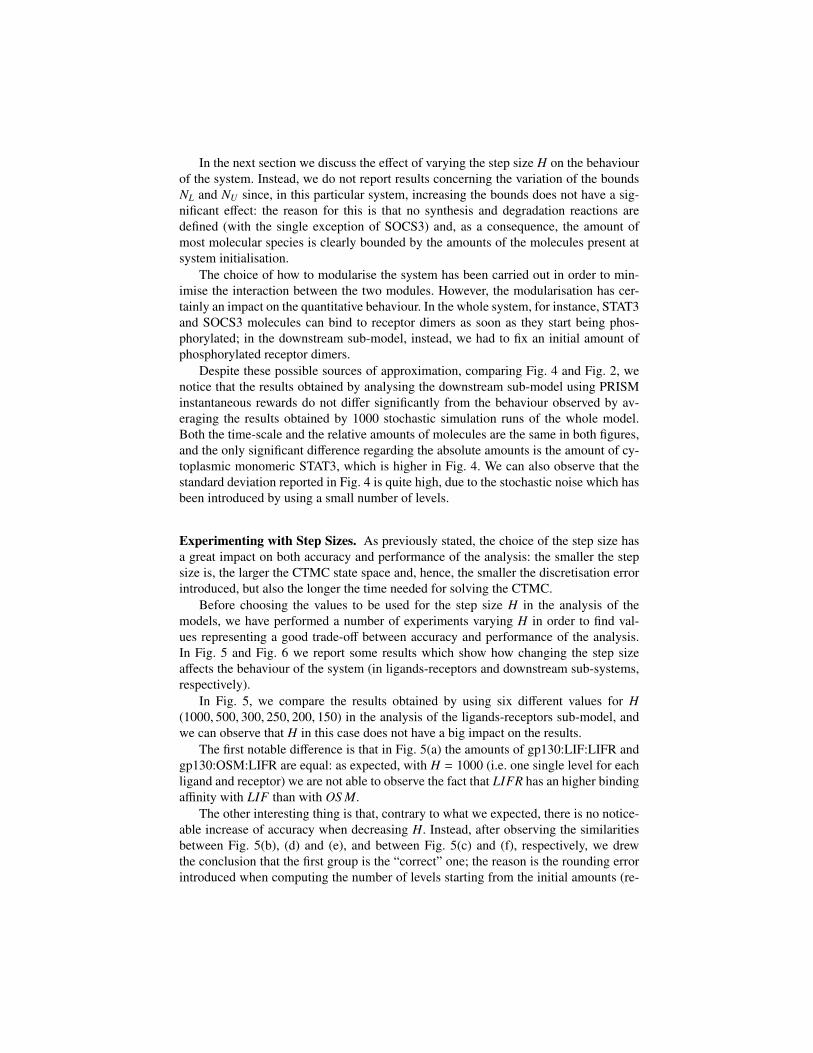
Before choosing the values to be used for the step size H in the analysis of themodels, we have performed a number of experiments varying H in order to find val-ues representing a good trade-off between accuracy and performance of the analysis.In Fig. 5 and Fig. 6 we report some results which show how changing the step sizeaffects the behaviour of the system (in ligands-receptors and downstream sub-systems,respectively).

In Fig. 5, we compare the results obtained by using six different values for H(1000, 500, 300, 250, 200, 150) in the analysis of the ligands-receptors sub-model, andwe can observe that H in this case does not have a big impact on the results.

The first notable difference is that in Fig. 5(a) the amounts of gp130:LIF:LIFR andgp130:OSM:LIFR are equal: as expected, with H = 1000 (i.e. one single level for eachligand and receptor) we are not able to observe the fact that LIFR has an higher bindingaffinity with LIF than with OS M.

The other interesting thing is that, contrary to what we expected, there is no notice-able increase of accuracy when decreasing H. Instead, after observing the similaritiesbetween Fig. 5(b), (d) and (e), and between Fig. 5(c) and (f), respectively, we drewthe conclusion that the first group is the “correct” one; the reason is the rounding errorintroduced when computing the number of levels starting from the initial amounts (re-

0

100

200

300

400

500

0 5 10 15 20 25 30

Num

ber

of m

olec

ules

Time (minutes)

(a) H=1000

0

100

200

300

400

500

0 5 10 15 20 25 30

Num

ber

of m

olec

ules

Time (minutes)

(b) H=500

0

100

200

300

400

500

0 5 10 15 20 25 30

Num

ber

of m

olec

ules

Time (minutes)

(c) H=300

0

100

200

300

400

500

0 5 10 15 20 25 30

Num

ber

of m

olec

ules

Time (minutes)

(d) H=250

0

100

200

300

400

500

0 5 10 15 20 25 30

Num

ber

of m

olec

ules

Time (minutes)

(e) H=200

0

100

200

300

400

500

0 5 10 15 20 25 30

Num

ber

of m

olec

ules

Time (minutes)

(f) H=150

Fig. 5. Time-series by model-checking: ligands-receptors sub-model. The three typesof receptor complexes are shown, gp130:LIF:LIFR (red), gp130:OSM:LIFR (green),and gp130:OSM:OSMR (blue), in the stage when one (full line) or both (dashed line)receptors are phosphorylated.

member that NL = bMIN/Hc and NU = bMAX/Hc): when a small numbers of levels isused, this rounding error happens to be more significant than H itself.

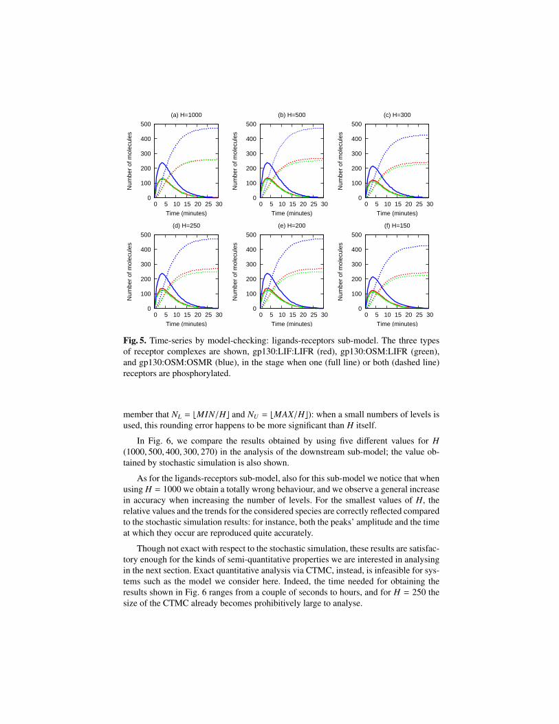
In Fig. 6, we compare the results obtained by using five different values for H(1000, 500, 400, 300, 270) in the analysis of the downstream sub-model; the value ob-tained by stochastic simulation is also shown.

As for the ligands-receptors sub-model, also for this sub-model we notice that whenusing H = 1000 we obtain a totally wrong behaviour, and we observe a general increasein accuracy when increasing the number of levels. For the smallest values of H, therelative values and the trends for the considered species are correctly reflected comparedto the stochastic simulation results: for instance, both the peaks’ amplitude and the timeat which they occur are reproduced quite accurately.

Though not exact with respect to the stochastic simulation, these results are satisfac-tory enough for the kinds of semi-quantitative properties we are interested in analysingin the next section. Exact quantitative analysis via CTMC, instead, is infeasible for sys-tems such as the model we consider here. Indeed, the time needed for obtaining theresults shown in Fig. 6 ranges from a couple of seconds to hours, and for H = 250 thesize of the CTMC already becomes prohibitively large to analyse.

0

500

1000

1500

2000

2500

3000

0 100 200 300 400 500 600 700 800

Num

ber

of m

olec

ules

Time (minutes)

(a) STAT_c

SimulationMC, H=1000MC, H=500

MC, H=400MC, H=300MC, H=270

0

20

40

60

80

100

120

0 100 200 300 400 500 600 700 800

Num

ber

of m

olec

ules

Time (minutes)

(b) STAT3-PD_c

SimulationMC, H=1000MC, H=500

MC, H=400MC, H=300MC, H=270

0

50

100

150

200

250

300

350

400

450

500

0 100 200 300 400 500 600 700 800

Num

ber

of m

olec

ules

Time (minutes)

(c) STAT3_n

SimulationMC, H=1000MC, H=500MC, H=400MC, H=300MC, H=270

0

100

200

300

400

500

600

700

0 100 200 300 400 500 600 700 800

Num

ber

of m

olec

ules

Time (minutes)

(d) STAT3-PD_n

SimulationMC, H=1000MC, H=500MC, H=400MC, H=300MC, H=270

Fig. 6. Time-series by model-checking: STAT3 sub-model.

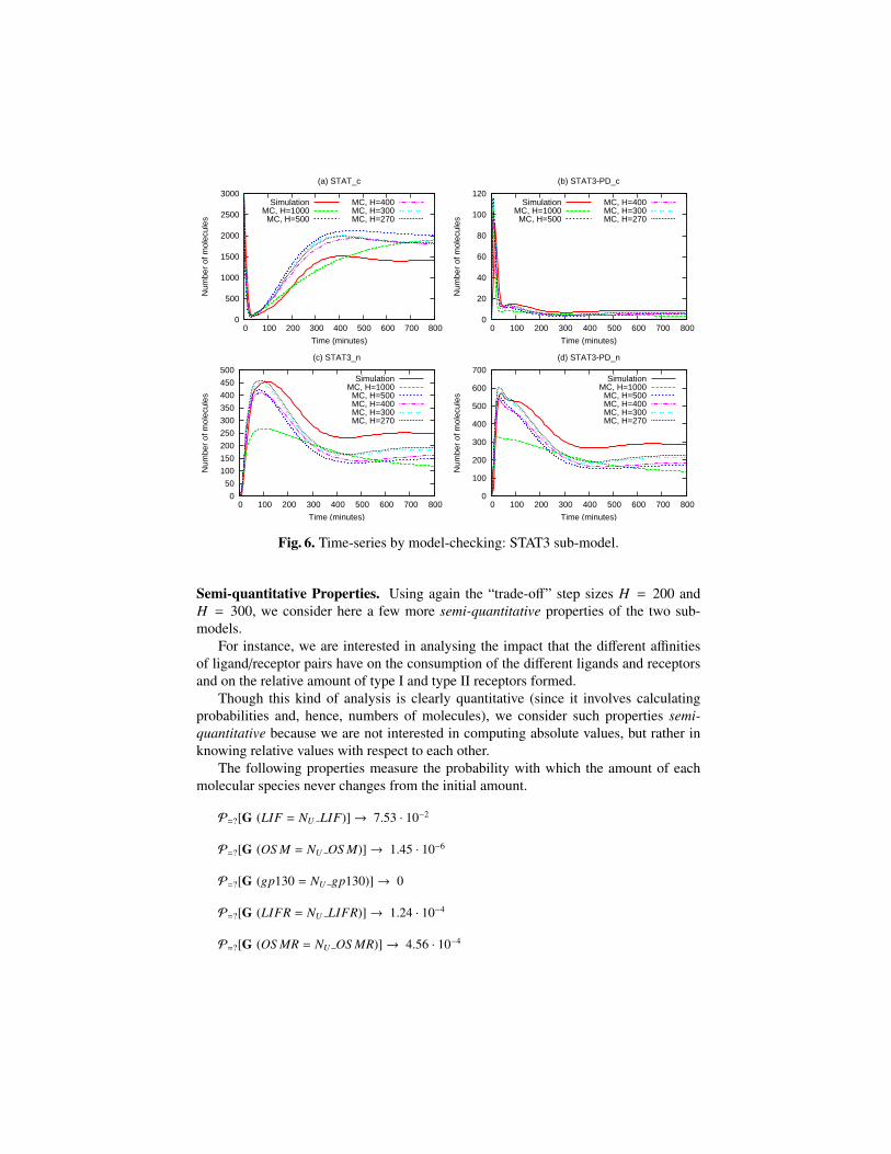
Semi-quantitative Properties. Using again the “trade-off” step sizes H = 200 andH = 300, we consider here a few more semi-quantitative properties of the two sub-models.

For instance, we are interested in analysing the impact that the different affinitiesof ligand/receptor pairs have on the consumption of the different ligands and receptorsand on the relative amount of type I and type II receptors formed.

Though this kind of analysis is clearly quantitative (since it involves calculatingprobabilities and, hence, numbers of molecules), we consider such properties semi-quantitative because we are not interested in computing absolute values, but rather inknowing relative values with respect to each other.

The following properties measure the probability with which the amount of eachmolecular species never changes from the initial amount.

P=?[G (LIF = NU LIF)]→ 7.53 · 10−2

P=?[G (OS M = NU OS M)]→ 1.45 · 10−6

P=?[G (gp130 = NU gp130)]→ 0

P=?[G (LIFR = NU LIFR)]→ 1.24 · 10−4

P=?[G (OS MR = NU OS MR)]→ 4.56 · 10−4

From the obtained results we notice, for instance, that gp130 is always used (indeed,it is necessary to form all receptor dimers), and that it is more likely for OSM to beconsumed than LIF (indeed, LIF is only used in the formation of one type of receptordimers).

We measure also the probability with which the amount of each molecular speciesreaches its lower bound.

This group of properties shows that gp130 is totally consumed in any possible evo-lution of the system, that LIF and OSM are never totally consumed, and that the prob-ability of LIFR being totally consumed is equal to the probability of OSMR not beingused at all. These results mean that gp130 is the bottleneck of the system, while LIFand OSM are present in abundance.

P=?[F (LIF = NL LIF)]→ 0

P=?[F (OS M = NL OS M)]→ 0

P=?[F (gp130 = NL gp130)]→ 1

P=?[F (LIFR = NL LIFR)]→ 4.56 · 10−4

P=?[F (OS MR = NL OS MR)]→ 1.24 · 10−4

Finally, we consider the reward-based property

Ri=?[C ≤ T ]

and we verify it on the downstream sub-model for time points T ≤ 800 minutes, wherei is an integer variable referring to a transition reward structure.

In addition to state rewards, in fact, PRISM allows for the definition of reward struc-tures which associate with each transition a cumulative reward equal to its expectednumber of occurrences up to the considered time.

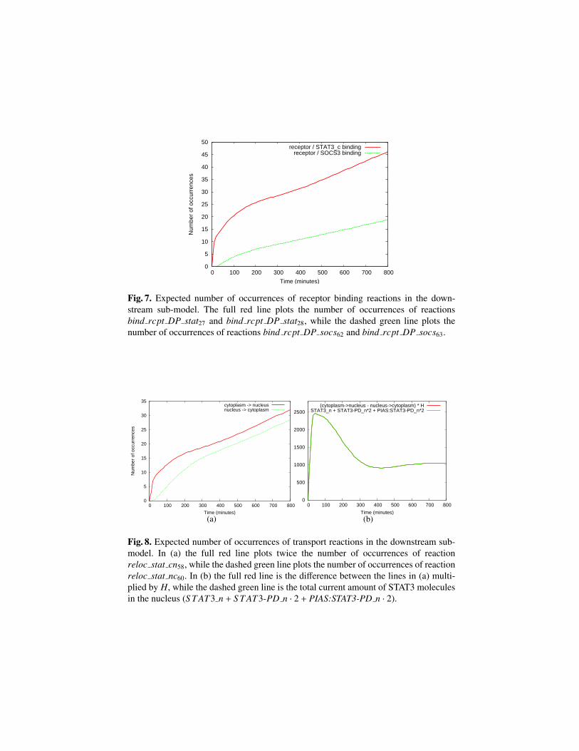
In Fig. 7 and Fig. 8 the expected number of occurrences for some of the reactionsof the downstream sub-model is shown.

In particular, in Fig. 7 we compare the number of occurrences of receptors/STAT3and receptors/SOCS3 binding reactions, which shows intuitively the different bindingaffinities of STAT3 and SOCS3 to the receptor dimers.

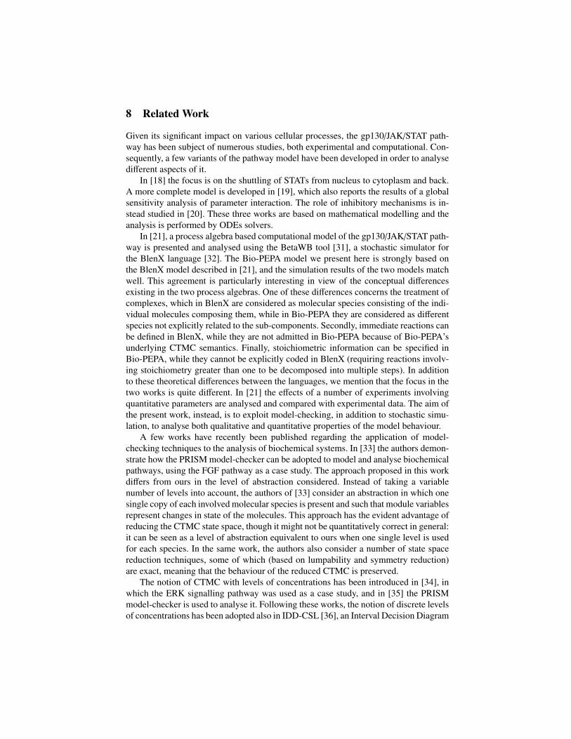
In Fig. 8, instead, we consider the number of occurrences of transport reactions ofSTAT3 molecules from cytoplasm to nucleus and back. In Fig. 8(a) we compare thenumber of occurrences of transport in the two directions: we count each transport fromcytoplasm to nucleus twice since STAT3 molecules are translocated in the nucleus indimeric form and, hence, a pair of STAT3 molecules is moved at each reaction occur-rence. We observe that, since at system initialisation no STAT3 molecule is present inthe nucleus, the difference between the two curves in Fig. 8(a) (multiplied by the stepsize H) must be the number of STAT3 molecules present in the nucleus. This consider-ation is confirmed by the perfect agreement of the two curves in Fig. 8(b).

0

5

10

15

20

25

30

35

40

45

50

0 100 200 300 400 500 600 700 800

Num

ber

of o

ccur

renc

es

Time (minutes)

receptor / STAT3_c bindingreceptor / SOCS3 binding

Fig. 7. Expected number of occurrences of receptor binding reactions in the down-stream sub-model. The full red line plots the number of occurrences of reactionsbind rcpt DP stat27 and bind rcpt DP stat28, while the dashed green line plots thenumber of occurrences of reactions bind rcpt DP socs62 and bind rcpt DP socs63.

0

5

10

15

20

25

30

35

0 100 200 300 400 500 600 700 800

Num

ber

of o

ccur

renc

es

Time (minutes)

cytoplasm -> nucleusnucleus -> cytoplasm

(a)

0

500

1000

1500

2000

2500

0 100 200 300 400 500 600 700 800

Time (minutes)

(cytoplasm->nucleus - nucleus->cytoplasm) * HSTAT3_n + STAT3-PD_n*2 + PIAS:STAT3-PD_n*2

(b)

Fig. 8. Expected number of occurrences of transport reactions in the downstream sub-model. In (a) the full red line plots twice the number of occurrences of reactionreloc stat cn58, while the dashed green line plots the number of occurrences of reactionreloc stat nc60. In (b) the full red line is the difference between the lines in (a) multi-plied by H, while the dashed green line is the total current amount of STAT3 moleculesin the nucleus (S T AT3 n + S T AT3-PD n · 2 + PIAS:STAT3-PD n · 2).

8 Related Work

Given its significant impact on various cellular processes, the gp130/JAK/STAT path-way has been subject of numerous studies, both experimental and computational. Con-sequently, a few variants of the pathway model have been developed in order to analysedifferent aspects of it.

In [18] the focus is on the shuttling of STATs from nucleus to cytoplasm and back.A more complete model is developed in [19], which also reports the results of a globalsensitivity analysis of parameter interaction. The role of inhibitory mechanisms is in-stead studied in [20]. These three works are based on mathematical modelling and theanalysis is performed by ODEs solvers.

In [21], a process algebra based computational model of the gp130/JAK/STAT path-way is presented and analysed using the BetaWB tool [31], a stochastic simulator forthe BlenX language [32]. The Bio-PEPA model we present here is strongly based onthe BlenX model described in [21], and the simulation results of the two models matchwell. This agreement is particularly interesting in view of the conceptual differencesexisting in the two process algebras. One of these differences concerns the treatment ofcomplexes, which in BlenX are considered as molecular species consisting of the indi-vidual molecules composing them, while in Bio-PEPA they are considered as differentspecies not explicitly related to the sub-components. Secondly, immediate reactions canbe defined in BlenX, while they are not admitted in Bio-PEPA because of Bio-PEPA’sunderlying CTMC semantics. Finally, stoichiometric information can be specified inBio-PEPA, while they cannot be explicitly coded in BlenX (requiring reactions involv-ing stoichiometry greater than one to be decomposed into multiple steps). In additionto these theoretical differences between the languages, we mention that the focus in thetwo works is quite different. In [21] the effects of a number of experiments involvingquantitative parameters are analysed and compared with experimental data. The aim ofthe present work, instead, is to exploit model-checking, in addition to stochastic simu-lation, to analyse both qualitative and quantitative properties of the model behaviour.

A few works have recently been published regarding the application of model-checking techniques to the analysis of biochemical systems. In [33] the authors demon-strate how the PRISM model-checker can be adopted to model and analyse biochemicalpathways, using the FGF pathway as a case study. The approach proposed in this workdiffers from ours in the level of abstraction considered. Instead of taking a variablenumber of levels into account, the authors of [33] consider an abstraction in which onesingle copy of each involved molecular species is present and such that module variablesrepresent changes in state of the molecules. This approach has the evident advantage ofreducing the CTMC state space, though it might not be quantitatively correct in general:it can be seen as a level of abstraction equivalent to ours when one single level is usedfor each species. In the same work, the authors also consider a number of state spacereduction techniques, some of which (based on lumpability and symmetry reduction)are exact, meaning that the behaviour of the reduced CTMC is preserved.

The notion of CTMC with levels of concentrations has been introduced in [34], inwhich the ERK signalling pathway was used as a case study, and in [35] the PRISMmodel-checker is used to analyse it. Following these works, the notion of discrete levelsof concentrations has been adopted also in IDD-CSL [36], an Interval Decision Diagram

based model-checker for stochastic Petri nets, which allows for the verification of CSLproperties.

In [37] the authors propose a framework, based on Petri nets, in which qualitativeand quantitative (stochastic and continuous) analysis of biochemical pathways are inte-grated. Qualitative properties such as boundedness, liveness and reversibility are con-sidered, in addition to the possibility to check for P- and T-invariants, and behaviouralproperties are verified by probabilistic model-checking.

Finally, BIOCHAM [38, 39] is a framework for modelling, simulating and analysingbiochemical systems, in which different semantics (differential, stochastic, discrete, andboolean) are considered. BIOCHAM allows for the verification of temporal proper-ties expressed in the Computation Tree Logic (CTL) by using the NuSMV model-checker [40].

9 Conclusions and Future Work

In this work we have used the gp130/JAK/STAT signalling pathway as a case studyfor modelling and analysis using the Bio-PEPA process algebra. Among the possibleanalysis methods made available by the Bio-PEPA Workbench, we have consideredstochastic simulation and model-checking.

The results obtained by simulation agree well with existing mathematical and com-putational models. The application of the model-checking approach to the analysis ofthe pathway model, though limited by the state space explosion problem, provided uswith some useful insight. First, it can be used for consistency checking, in order to guar-antee the satisfaction of essential properties and, therefore, the absence of modelling er-rors. Second, it allows us to check for the satisfaction of semi-quantitative behaviouralproperties over the whole model, without the need for computing average values over anumber of stochastic simulation runs.

In order to deal with the computational complexity of model-checking, we havesubdivided the pathway model into two distinct sub-models. The time-series analysisobtained by analysing the sub-models individually via model-checking shows a reason-ably good agreement with the behaviour obtained via stochastic simulation. The issueof modularisation of models of biochemical systems is a complex one. In this workwe have adopted a simple approach which is adequate for this particular case study. Ageneral approach for modularisation of models deserves additional study, in particularin view of the possible performance improvement which this technique could bring inmodel-checking.

Finally, in order to fully exploit the framework provided by Bio-PEPA further anal-ysis could be performed on the MATLAB model generated by the Bio-PEPA Work-bench using ODEs based methods to perform, for instance, bifurcation, stability, andcontinuation analysis.

Acknowledgments. The author wishes to thank Jane Hillston for her helpful com-ments. This research is supported by the EPSRC grant EP/E031439/1 “Stochastic Pro-cess Algebra for Biochemical Signalling Pathway Analysis”.

References

1. Regev, A., Silverman, W., Shapiro, E.: Representation and simulation of biochemical pro-cesses using the π-calculus process algebra. In: Proceedings of Pacific Symposium on Bio-computing (PSB’01). Volume 6. (2001) 459–470

2. Regev, A., Panina, E.M., Silverman, W., Cardelli, L., Shapiro, E.Y.: BioAmbients: an Ab-straction for Biological Compartments. Theoretical Computer Science 325(1) (2004) 141–167

3. Cardelli, L.: Brane Calculi - Interactions of Biological Membranes. In: Proceedings ofComputational Methods in Systems Biology (CMSB’04). Volume 3082 of LNCS. (2005)257–278

4. Priami, C., Quaglia, P.: Operational patterns in Beta-binders. Transactions on ComputationalSystems Biology 1 (2005) 50–65

5. Danos, V., Laneve, C.: Formal molecular biology. TCS 325(1) (2004)6. Regev, A., Shapiro, E.: Cells as Computation. Nature 419(6905) (2002) 3437. Ciocchetta, F., Hillston, J.: Bio-PEPA: an extension of the process algebra PEPA for bio-

chemical networks. In: Proc. of FBTC’07. Volume 194 of ENTCS. (2008) 103–1178. Ciocchetta, F., Hillston, J.: Bio-PEPA: a Framework for the Modelling and Analysis of

Biochemical Networks. Theoretical Computer Science (2009, in press)9. Hillston, J.: A Compositional Approach to Performance Modelling. Cambridge University

Press (1996)10. Ciocchetta, F., Hillston, J.: Calculi for Biological Systems. In: Formal Methods for Computa-

tional Systems Biology (SFM’08). Volume 5016 of LNCS. Springer-Verlag (2008) 265–31211. Bio-PEPA Workbench Home Page: http://www.dcs.ed.ac.uk/home/stg/software/biopepa/

12. Ramsey, S., Orrell, D., Bolouri, H.: Dizzy: stochastic simulation of large-scale genetic reg-ulatory networks. J. Bioinf. Comp. Biol. 3(2) (2005) 415–436

13. PRISM Home Page: http://www.prismmodelchecker.org14. Aziz, A., Sanwal, K., Singhal, V., Brayton, R.: Model-checking continuous-time Markov

chains. ACM Trans. Comput. Logic 1(1) (2000) 162–17015. Underhill-Day, N., Heath, J.: Oncostatin M (OSM) Cytostasis of Breast Tumor Cells: Char-

acterization of an OSM Receptor β-Specific Kernel. Cancer Research 66(22) (2006) 10891–10901

16. Heinrich, P., Behrmann, I., Haan, S., Hermanns, H., Muller-Newen, G., Schaper, F.: Princi-ples od interleukin (IL)-6-type cytokine signalling and its regulation. Biochem. J. 374 (2003)1–20

17. Kisseleva, T., Bhattacharya, S., Braunstein, J., Schindler, C.: Signaling through theJAK/STAT pathway, recent advances and future challenges. Gene 285 (2002) 1–24

18. Swameye, I., Muller, T., Timmer, J., Sandra, O., Klingmuller, U.: Identification of nucleo-cytoplasmic cycling as a remote sensor in cellular signaling by databased modeling. PNAS100 (2003) 1028–1033

19. Mahdavi, A., Davey, R.E., Bhola, P., Yin, T., Zandstra, P.W.: Sensitivity Analysis of In-tracellular Signaling Pathway Kinetics Predicts Targets for Stem Cell Fate Control. PLoSComputational Biology 3(7) (2007) 1257–1267

20. Singh, A., Jayaraman, A., Hahn, J.: Modeling Regulatory Mechanisms in IL-6 Transductionin Hepatocytes. Biotechnology and Bioengineering 95(5) (2006) 850–862

21. Guerriero, M.L., Dudka, A., Underhill-Day, N., Heath, J.K., Priami, C.: Narrative-basedcomputational modelling of the Gp130/JAK/STAT signalling pathway. BMC Systems Biol-ogy 3(1) (2009) 40

22. Bio-PEPA Home Page: http://www.biopepa.org/

23. Hinton, A., Kwiatkowska, M., Norman, G., Parker, D.: PRISM: A tool for automatic verifi-cation of probabilistic systems. In: Proc. 12th International Conference on Tools and Algo-rithms for the Construction and Analysis of Systems (TACAS’06). Volume 3920 of LNCS.,Springer (2006) 441–444

24. Dizzy Home Page: http://magnet.systemsbiology.net/software/Dizzy25. Aziz, A., Kanwal, K., Singhal, V., Brayton, V.: Verifying continuous time Markov chains.

In: Proc. 8th International Conference on Computer Aided Verification (CAV’96). Volume1102 of LNCS., Springer (1996) 269–276

26. Baier, C., Katoen, J.P., Hermanns, H.: Approximate Symbolic Model Checking ofContinuous-Time Markov Chains. In: Proceedings of CONCUR’99. Volume 1664 of LNCS.(1999) 146–161

27. Saez-Rodriguez, J. Kremling, A., Gilles, E.: Dissecting the puzzle of life: modularization ofsignal transduction networks. Computers and Chemical Engineering 29 (2005) 619–629

28. Conzelmann, H., Saez-Rodriguez, J., Sauter, T., Bullinger, E., Allgower, F., Gilles, E.: Re-duction of mathematical models of signal transduction networks: simulation-based approachapplied to EGF receptor signalling. Systems Biology 1(1) (2004) 159–169

29. Monteiro, P., Ropers, D., Mateescu, R., Freitas, A., de Jong, H.: Temporal logic patterns forquerying dynamic models of cellular interaction networks. ECCB 24 (2008) 227–233

30. Gibson, M., Bruck, J.: Efficient Exact Stochastic Simulation of Chemical Systems withMany Species and Many Channels. The Journal of Chemical Physics 104 (2000) 1876–1889

31. Dematte, L., Priami, C., Romanel, A.: The Beta Workbench: a computational tool to studythe dynamics of biological systems. Briefings in Bioinformatics 9(5) (2008) 437–449 (Toolavailable at http://www.cosbi.eu/Rpty_Soft_BetaWB.php).

32. Dematte, L., Priami, C., Romanel, A.: The BlenX Language: A Tutorial. In: Formal Meth-ods for Computational Systems Biology (SFM’08). Volume 5016 of LNCS. Springer-Verlag(2008) 313–365

33. Heath, J., Kwiatkowska, M., Norman, G., Parker, D., Tymchyshyn, O.: Probabilistic ModelChecking of Complex Biological Pathways. Theoretical Computer Science 319 (2008) 239–257

34. Calder, M., Gilmore, S., Hillston, J.: Modelling the Influence of RKIP on the ERK SignallingPathway Using the Stochastic Process Algebra PEPA. Transactions on Computational Sys-tems Biology (Proc of BioConcur’04) 7 (2006) 1–23

35. Calder, M., Vyshemirsky, V., Gilbert, D., Orton, R.: Analysis of signalling pathways usingcontinuous time Markov chains. Transactions on Computational Systems Biology 6 (2006)44–67

36. The Idd-CSL Home Page: http://www-dssz.informatik.tu-cottbus.de/

software/software.html

37. Heiner, M., Gilbert, D., Donaldson, R.: Petri Nets for Systems and Synthetic Biology. In:Formal Methods for Computational Systems Biology (SFM’08). Volume 5016 of LNCS.Springer-Verlag (2008) 215–264

38. The BIOCHAM Home Page: http://contraintes.inria.fr/BIOCHAM/

39. Fages, F., Soliman, S., Chabrier-Rivier, N.: Modelling and querying interaction networks inthe biochemical abstract machine BIOCHAM. Journal of Biological Physics and Chemistry4(2) (2004) 64–73

40. NuSMV Home Page: http://nusmv.irst.itc.it/