UNIVERSITA DEGLI STUDI DI TRENTO - …homepages.inf.ed.ac.uk/jeh/Bio-PEPA/Ellavarason_Thesis_FINAL.pdf · UNIVERSITA DEGLI STUDI DI TRENTO Facolt a di Scienze Matematiche, Fisiche

UNIVERSITA DEGLI STUDI DI TRENTOFacolta di Scienze Matematiche, Fisiche e Naturali

Corso di Laurea Specialistica in InformaticaWithin European Masters in Informatics

Tesi di Laurea

An Automatic Mapping from the Systems

Biology Markup Language to the Bio-PEPA

Process Algebra

Relatori Laureanda

Prof. Corrado Priami Kanimozhi EllavarasonFederica Ciocchetta

Anno Accademico 2007/2008

Abstract

This dissertation concerns the automatic mapping of the Systems Biology

Markup Language (SBML) into the Bio-PEPA process algebra. SBML is

considered the standard for the representation, collection and exchange of

biological models. Bio-PEPA is a process algebra recently defined for the

modelling and analysis of biochemical systems.

We develop a theoretical mapping from SBML models to Bio-PEPA systems.

This is accompanied by a Java based software tool, called SBML2BioPEPA,

for implementing the translation in practice. The software tool is able to suc-

cessfully convert SBML models into the equivalent Bio-PEPA models. These

models can then be analysed and simulated in the various tools available for

Bio-PEPA models such as the Bio-PEPA Eclipse Plugin. We consider two

case studies of biochemical networks to test and validate our mapping and

software tool. The results we obtain are in agreement with the published re-

sults for the biological networks and with the results obtained by importing

the SBML models in the COPASI software tool.

Our work allows translation of SBML models to Bio-PEPA with ease. This

lets researchers take advantage of the various analysis methods and software

tools available for Bio-PEPA models.

i

ii

Acknowledgements

First and foremost, I would like to praise God for giving me the grace and

blessing to get enrolled into EuMI course and giving me the strength to

complete it. I have no words to thank my loving family back in India who

supported me with my decision to go abroad and study. They always made

me feel so close to them with their love.

I would like to thank Prof. Jane Hillston for letting me work on this

interesting topic. My genuine thanks to Federica, who guided me in this

thesis work. I would also like to thank Prof. Corrado Priami for supervising

my thesis from Trento side.

My sincere thanks to all the EuMI staff in University of Edinburgh and

University of Trento for I learned so much at these renowned universities. A

huge thanks to all my friends for being part of these wonderful two years.

And lastly, I dedicate this thesis to my soulmate...Amby. Your immense

Love has been has been my driving force and I know it will stay on for a

lifetime! Heartfelt thanks to you, as I was able to achieve all this because of

your infinite support!

iii

iv

Contents

1 Introduction 1

1.1 Introduction . . . . . . . . . . . . . . . . . . . . . . . . . . . . 1

1.2 Motivations . . . . . . . . . . . . . . . . . . . . . . . . . . . . 2

1.3 Objectives . . . . . . . . . . . . . . . . . . . . . . . . . . . . . 4

1.4 Structure of Dissertation . . . . . . . . . . . . . . . . . . . . . 4

2 Background 6

2.1 Systems Biology Markup Language . . . . . . . . . . . . . . . 6

2.1.1 Standards in Systems Biology . . . . . . . . . . . . . . 7

2.1.2 SBML model definition . . . . . . . . . . . . . . . . . . 8

2.1.3 Example SBML model . . . . . . . . . . . . . . . . . . 13

2.2 Process Algebras . . . . . . . . . . . . . . . . . . . . . . . . . 15

2.3 Bio-PEPA . . . . . . . . . . . . . . . . . . . . . . . . . . . . . 16

2.3.1 Bio-PEPA Syntax . . . . . . . . . . . . . . . . . . . . . 18

2.3.2 Operational Semantics . . . . . . . . . . . . . . . . . . 20

2.3.3 Example model using Bio-PEPA . . . . . . . . . . . . . 21

2.4 Software tools . . . . . . . . . . . . . . . . . . . . . . . . . . 23

2.5 Related Work . . . . . . . . . . . . . . . . . . . . . . . . . . . 24

3 Mapping from SBML to Bio-PEPA 26

3.1 Elements of Bio-PEPA model . . . . . . . . . . . . . . . . . . 26

3.2 The Mapping . . . . . . . . . . . . . . . . . . . . . . . . . . . 27

v

3.2.1 Compartments . . . . . . . . . . . . . . . . . . . . . . 28

3.2.2 Species . . . . . . . . . . . . . . . . . . . . . . . . . . . 29

3.2.3 Parameters . . . . . . . . . . . . . . . . . . . . . . . . 30

3.2.4 Functional Rates . . . . . . . . . . . . . . . . . . . . . 32

3.2.5 Species Components . . . . . . . . . . . . . . . . . . . 34

3.2.6 Model Component . . . . . . . . . . . . . . . . . . . . 36

3.3 Limitations of the Mapping . . . . . . . . . . . . . . . . . . . 37

3.4 Summary of Mapping . . . . . . . . . . . . . . . . . . . . . . . 38

4 Software Tool 39

4.1 Development Tools . . . . . . . . . . . . . . . . . . . . . . . . 39

4.2 Java Classes Design . . . . . . . . . . . . . . . . . . . . . . . . 40

4.3 Tool Deployment . . . . . . . . . . . . . . . . . . . . . . . . . 43

5 Case Studies 45

5.1 Repressilator - A Synthetic Oscillatory Network . . . . . . . . 46

5.1.1 Description of the model . . . . . . . . . . . . . . . . . 46

5.1.2 Mapping Description . . . . . . . . . . . . . . . . . . . 47

5.1.3 Simulation of Bio-PEPA Repressilator model . . . . . . 53

5.2 Mitogen Activated Proetin Kinases Model . . . . . . . . . . . 55

5.2.1 Description of the model . . . . . . . . . . . . . . . . . 55

5.2.2 Mapping Description . . . . . . . . . . . . . . . . . . . 56

5.2.3 Simulation of Bio-PEPA MAPK model . . . . . . . . . 63

6 Conclusions 65

6.1 Concluding remarks . . . . . . . . . . . . . . . . . . . . . . . . 65

6.2 Further Work . . . . . . . . . . . . . . . . . . . . . . . . . . . 66

A Bio-PEPA model for the Repressilator pathway 68

B Bio-PEPA model for the MAPK pathway 71

vi

C Bio-PEPA model syntax for Eclipse Plugin 75

vii

viii

List of Figures

4.1 Main classes used in the SBML2BioPEPA software tool . . . . 41

5.1 Schematic diagram of the Represillator . . . . . . . . . . . . . 46

5.2 Stochastic simulation results of oscillations in Repressilator

network using Bio-PEPA plugin. . . . . . . . . . . . . . . . . . 53

5.3 Stochastic simulation results of oscillations in Repressilator

network using COPASI tool . . . . . . . . . . . . . . . . . . . 54

5.4 The Mitogen Activated Protein Kinase cascade . . . . . . . . 56

5.5 Stochastic simulation results of MAPK using Bio-PEPA Plugin 63

5.6 Stochastic simulation results of MAPK using COPASI tool . . 64

ix

x

List of Tables

2.1 Operational semantics for Bio-PEPA . . . . . . . . . . . . . . 20

3.1 Summary of mapping from SBML to Bio-PEPA . . . . . . . . 38

5.1 List of Species in Repressilator model . . . . . . . . . . . . . . 48

5.2 List of Parameters in Repressilator model . . . . . . . . . . . . 49

5.3 List of Reactions in Repressilator model . . . . . . . . . . . . 50

5.4 List of Species in MAPK model . . . . . . . . . . . . . . . . . 57

5.5 List of Parameters in MAPK model . . . . . . . . . . . . . . . 58

5.6 List of Reactions in MAPK model . . . . . . . . . . . . . . . . 60

xi

xii

Chapter 1

Introduction

This chapter presents an introduction to the main topics of the thesis. The

thesis is devoted to the design and development of a software tool for auto-

matic translation of models from Systems Biology Markup Language (SBML)

to the process algebra Bio-PEPA. After an introduction to the context of ap-

plication of our work, we describe the motivation of our research and the

objectives we aim to achieve. Finally, the structure of the thesis is reported.

1.1 Introduction

Molecular biology techniques have unveiled enormous amounts of informa-

tion on genes and proteins. The information obtained is at the molecular

level. At the system level, genes and proteins interact in a very complex

fashion. The challenge is now to understand the functions and the behaviour

of the system as a whole. This is the aim of Systems Biology, a relatively new

field of study. As described in [1], ‘Systems biology deals with the systems

level understanding of the interactions in the biological systems’.

Computational modelling and simulation of biological pathways are impor-

tant research aspects in systems biology. ‘They can help us understand the

internal nature and the dynamics of the process and arrive at well founded

1

predictions about the future developments’ [2]. There are numerous tech-

niques for the modelling and analysis of biological systems. Some of the

important techniques that have been used for modelling are ordinary differ-

ential equations [3], Petri nets [4], process algebras [5], Boolean networks [6]

and graph based approaches [7].

Recently, there has been increasing interest in the application of process al-

gebras in the field of systems biology [8], [9], [10], [11], [12], [13], [14], [15],

[16]. Process algebras are mathematical formalisms originally defined for the

modelling and analysis of concurrent systems [5], [17]. The entities such as

ion or molecules in the biosystems interact in a concurrent fashion. Hence,

the various species can be abstracted in a process algebra context by pro-

cesses interacting with each other by means of actions [8]. Process algebra

formalisms are useful in systems biology as they offer a formal representa-

tion of the model, a compositional approach and support different kinds of

analysis. Examples of process algebras applied to biology are π-calculus [5],

stochastic-π calculus [19], Beta-binders [9], Performance Evaluation Process

Algebra (PEPA) [20] and Bio-PEPA [16]. Among the different process al-

gebras, in this dissertation we consider Bio-PEPA. Bio-PEPA extends the

process algebra PEPA with some constructs to render features of biochemi-

cal networks.

Another important research area in systems biology is the definition of a

standard for the representation of biochemical networks. Among the numer-

ous proposals, SBML [22] is emerging as the standard for the representation

and exchange of biological models. It is supported by many software tools

and has gained widespread acceptance [10].

1.2 Motivations

The aim of this dissertation is the definition of an automatic conversion of

models from SBML to Bio-PEPA. The main motivations of this work are

2

mentioned below:

• Among the different exchange languages available, SBML is emerging

as the standard for the representation of biological models. It provides

a way to exchange models between different softwares without the need

of re-encoding the model. It is well accepted and is in widespread use.

It is known to be supported by over 90 software packages. Further, a

lot of models have been collected in SBML format, such as the ones

in the Biomodels database [23]. Due to these reasons, we have chosen

SBML in our research.

• Process algebras are formalisms used to represent concurrent systems.

They have properties that make them particularly useful in the context

of systems biology such as compositionality, formal representation, sim-

ple abstraction and analysis. Among the different process algebras we

consider Bio-PEPA for our dissertation. There are various motivations

for this choice.

– Bio-PEPA is specifically designed for representing biochemical sys-

tems. In particular, it is possible to represent stoichiometry and

general kinetic-laws (different from mass-action).

– It supports numerous kinds of analysis and therefore allows us to

investigate the properties of the system from different compatible

views. We can perform stochastic and deterministic simulation,

check the formal properties of the system by using model checking

or consider other analysis based on continous time Markov chain

(CTMC).

• Bio-PEPA is a formal language and it is not straight-forward for non-

experts to model biosystems using its constructs. Developing a tool

for automatic conversion from SBML to Bio-PEPA will enable users to

generate Bio-PEPA models with ease. In this way the complexity of

the formalism can be hidden from the end user.

3

• The correctness of the tool can be tested by translating some well-

known SBML models into Bio-PEPA using our tool and performing

simulations on the translated models. The results obtained can then

be compared with the results published in the literature and the results

obtained by importing the same SBML models into other analysis tools

supporting SBML.

1.3 Objectives

The main goals of this dissertation are:

1. To present a formal translation from SBML to Bio-PEPA. We discuss

the theoretical mapping and also mention any assumptions we make.

2. To develop a Java based software tool for translation of the SBML

models to Bio-PEPA. The tool derives a Bio-PEPA specification cor-

responding to the SBML model. The syntax is the one that is used as

input for the Bio-PEPA plugin tool for analysis.

3. To generate Bio-PEPA models of biological systems found in literature

using the above tool. These models will then be simulated using the

Bio-PEPA plug-in and the obtained results will be compared with the

published ones. Furthermore, the model can be used to investigate

further properties and possible behaviours of the associated biological

system.

1.4 Structure of Dissertation

This chapter described the introduction, motivations and the objectives of

our work. The rest of the dissertation is structured as follows. Chapter 2

reviews the background of SBML with a description of its basic elements.

We also describe Bio-PEPA and its usage in modelling biological systems. In

4

Chapter 3, we put forward the theoretical mapping and assumptions for the

translation of models from SBML to Bio-PEPA. Chapter 4 talks about the

class design and data structures of the software tool which implements the

mapping. In Chapter 5, the results obtained using the software tool in two

case studies are elucidated. The results obtained are analysed and compared

with the literature. Finally, in Chapter 6, major conclusions of our work are

discussed and future work directions are proposed.

5

Chapter 2

Background

In this chapter we describe the background of our work. We begin by de-

scribing the necessity of standards for the representation of biological systems

followed by a detailed description of SBML and its components. A small ex-

ample of an SBML model is given in order to illustrate the language. We

then introduce process algebras and explain their advantages. The Bio-PEPA

syntax used for modelling biological systems is given along with a description

of semantics, and an example of a Bio-PEPA model is presented. We then

briefly mention the software tools we have used in our work. Finally, some

related works concerning the translation of SBML into process algebras are

reported.

2.1 Systems Biology Markup Language

The Systems Biology Markup Language (SBML) [22] is a machine-readable

format for describing qualitative and quantitative models of biochemical net-

works. SBML is based on the eXtensible Markup Language (XML) [24], a

popular text-based language for expressing structured data in a generic fash-

ion. It enables system biologists to share, evaluate and develop models coop-

eratively between different formalisms. The requirement of standard models

6

like SBML is described in the next subsection.

2.1.1 Standards in Systems Biology

Computational modelling techniques use various software tools for under-

standing the biological systems. There are many different formats of models

available. Systems biologists find it difficult to work with different formats.

The need of a standard representation of models is important in systems

biology because of the following reasons:

1. Users have to use multiple tools in their research. Different software

tools have different strengths and capabilities. However, these tools

cannot exchange their models because of having their own particular

representation formats.

2. Models that are published may use different modelling environments

and model representation languages. To use the model, users have to

manually translate the model into the particular formats they use.

3. Models could be stranded if simulation is not supported by the model

representation language. This will result in the loss of useful models.

A standard format representation is desirable in this case.

Due to these reasons, the need for the standard representation of models is

an important issue.

SBML has been developed in an effort to address the above problems. SBML

is evolving as a ‘de facto’ standard for the common representation of biologi-

cal models. In this way, the diversity of approaches used by different software

tools is acknowledged and a common format is followed. Among the different

exchange languages, SBML is the most known and used. The popularity of

SBML is growing in systems biology community as many software tools are

supporting it and models are being collected in model repositories such as

7

the BioModels database [23]. The SBML community continues to develop

and make software environments including programming libraries, conver-

sion utilities, interface packages for commonly used software environments

and easy to access online tools.

SBML is developed in levels; two levels have been defined so far. SBML

Level 1 is the basic version and has lesser representational power than SBML

Level 2 where the model definitions and mathematical expressions have been

enriched. Software tools that cannot or do not need to represent higher levels

can use Level 1. In this thesis, we have considered the latest available version

of SBML which is Level 2, Version 3.

2.1.2 SBML model definition

A biochemical network consists of compartments, species, reactions (includ-

ing reactants, products, reaction rate expressions and parameters).

SBML describes these components and additional information by using tags

and attributes [25]. A schema of an SBML model is presented below and

each component is described in detail.

<model id="My_Model" >

<listOfFunctionDefinitions>

...

</listOfFunctionDefinitions>

<listOfUnitDefinitions>

...

</listOfUnitDefinitions>

<listOfCompartments>

...

</listOfCompartments>

<listOfSpecies>

...

8

</listOfSpecies>

<listOfParameters>

...

</listOfParameters>

<listOfRules>

...

</listOfRules>

<listOfReactions>

...

<listOfReactants>

...

</listOfReactants>

<listOfProducts>

...

</listOfProducts>

<listOfModifiers>

...

</listOfModifiers>

<listOfLocalParameters>

...

</listOfLocalParameters>

</listOfReactions>

<listOfEvents>

...

</listOfEvents>

</model>

An SBML model definition consists of lists of SBML components. The

instances of the classes ListOfComponents must be located inside the tags

<listOfComponents> ... </listOfComponents>

9

where components could be FunctionDefinitions, UnitDefinitions, Com-

partments, Species, Parameters, Rules, Constraints, Reactions and

Events.

Although all lists are optional, if a given component is present in the model

then the corresponding list cannot be empty. The definition of one compo-

nent can have dependencies on other component definitions. For example,

the definition of reactions is built on other SBML elements, such as species

and compartments.

Mathematical expressions such as kinetic-laws, stoichiometry, events, func-

tions, rules occur in the model definition. The representation and semantic

interpretation is done using MathML [27] which is the international standard

for encoding mathematical expressions using XML.

We describe below the main SBML components and their principal tags and

attributes:

• Function definition - The mathematical functions that can be used in

the other part of the model are defined. Function defintions are done

using MathML expressions. Function definitions contain the following

important attributes:

1. Function definition id

2. MathML expression

• Unit definition - Units are mathematical entities that are specified ex-

plicitly. The definitions of sizes of the compartments, initial amounts

of species, constant units and variable parameter values have units as-

sociated with them. SBML defines units using built in functions. The

main attributes of unit definition are:

1. Unit id

2. Unit name

3. List of units

10

• Compartment - Species generally exist in a finite bound space known

as compartment. Every species that is defined in the model must be

located in a compartment. If there are any species defined in the model,

it is mandatory that at least one compartment type is defined. The

attributes of compartment are:

1. Compartment id

2. Compartment name

3. Compartment type

4. Compartment size

• Species - Simple entities (such as molecules or ions) that take part in a

chemical reaction are known as species. They are the reacting entities

of the specific species type. The initial quantity of the species are set

in the SBML file. If the quantity is missing, it is either unavailable or

set by an assignment rule. We list the important attributes that we

consider for the translation:

1. Species id

2. Species name

3. Species type

4. Compartment name

5. Initial concentration

• Reaction - Biochemical species interact with each other in reactions.

The speed of a reaction is expressed in terms of a rate-law involving

species and parameters. For each reaction the SBML model includes

the details about the species involved, their stoichiometric coefficients,

the parameters and the rate-law. The species can be reactants, prod-

ucts or modifiers (i.e. species which take part in a reaction but are

11

neither consumed nor produced as part of the reaction). The SBML

attributes and sub-tags for reaction are:

1. Reaction id

2. Reaction name

3. List of reactants and their stoichiometries

4. List of products and their stoichiometries

5. List of modifiers

6. Kinetic-law expressed by MathML expression

• Parameter - A parameter is a variable used in mathematical expres-

sions. Parameters in SBML can be of two kinds: global and local.

Parameters that are defined as global are available to the whole model.

The parameters defined as local are independent of the global param-

eters and are defined for particular reactions. The attributes are:

1. Parameter id

2. Parameter name

3. Parameter value

4. Parameter units

• Rule - Apart from the local and global parameters that are defined in

the model, rules provide a way of defining the value of variables in the

model, and the dynamic behaviour of those variables. Rules express

the relationships that cannot be expressed using reactions alone. The

list of attributes for rules are:

1. Variable name

2. MathML expression used to express the formula.

12

• Event - Events are constructs that represent changes in the system

due to some trigger conditions. During the evolution of the system,

events are evaluated using the mathematical formulas at specified time

intervals. It enables the modelling of various biological phenomena.

The attributes are:

1. Event id

2. Event name

3. Trigger

4. Delay

5. List of event assignments using MathML expressions

2.1.3 Example SBML model

Consider the system composed of species A, B, C and E involved in the

following reaction.

A+BE, k1[A][B]−−−−−−→ 2C

Here, A and B are the reactants, C is the product and E is the modifier.

[A] and [B] represent the concentrations of A and B respectively. The sto-

ichiometries of A, B and C are 1, 1 and 2 respectively. The sample SBML

file for this simple reaction is:

<?xml version="1.0" encoding="UTF-8"?>

<sbml xmlns="http://www.sbml.org/sbml/level2"

level="2" version="3">

<model id="SBMLsample" name="SBMLsample">

<listOfUnitDefinitions>

<unitDefinition id="time" name="minutes">

13

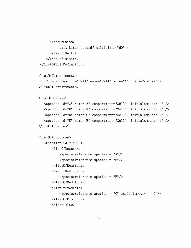
<listOfUnits>

<unit kind="second" multiplier="60" />

</listOfUnits>

</unitDefinition>

</listOfUnitDefinitions>

<listOfCompartments>

<compartment id="Cell" name="Cell" size="1" units="volume"/>

</listOfCompartments>

<listOfSpecies>

<species id="A" name="A" compartment="Cell" initialAmount="1" />

<species id="B" name="B" compartment="Cell" initialAmount="1" />

<species id="C" name="C" compartment="Cell" initialAmount="0" />

<species id="E" name="E" compartment="Cell" initialAmount="1" />

</listOfSpecies>

<listOfReactions>

<Reaction id = "R1">

<listOfReactants>

<speciesreference species = "A"/>

<speciesreference species = "B"/>

</listOfReactants>

<listOfModifiers>

<speciesreference species = "E"/>

</listOfModifiers>

<listOfProducts>

<speciesreference species = "C" stoichiometry = "2"/>

</listOfProducts>

<Kineticlaw>

14

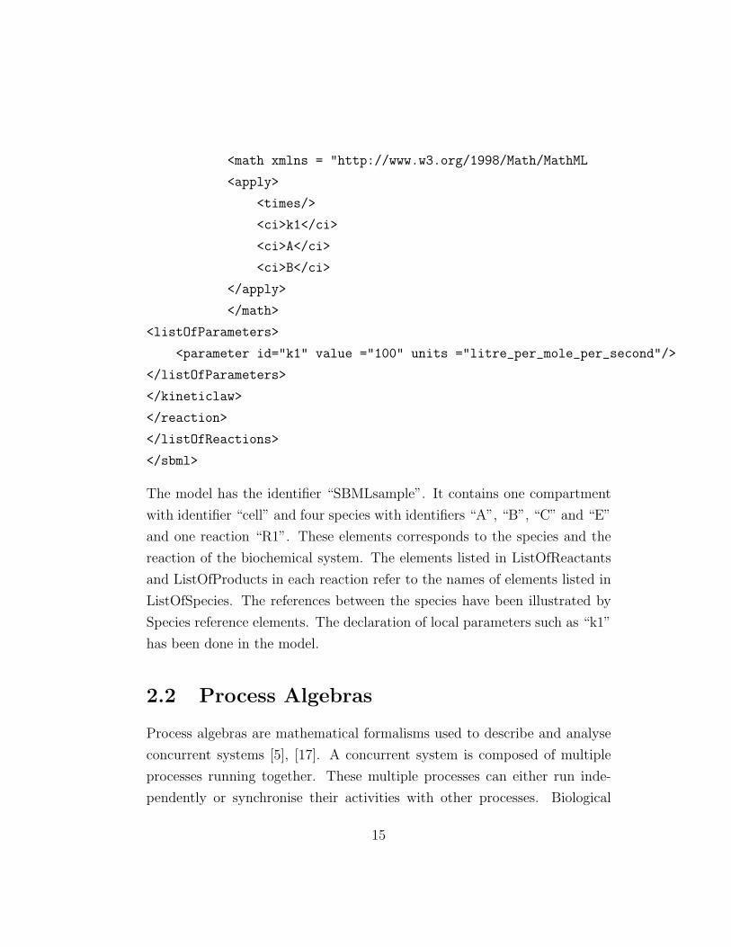
<math xmlns = "http://www.w3.org/1998/Math/MathML

<apply>

<times/>

<ci>k1</ci>

<ci>A</ci>

<ci>B</ci>

</apply>

</math>

<listOfParameters>

<parameter id="k1" value ="100" units ="litre_per_mole_per_second"/>

</listOfParameters>

</kineticlaw>

</reaction>

</listOfReactions>

</sbml>

The model has the identifier “SBMLsample”. It contains one compartment

with identifier “cell” and four species with identifiers “A”, “B”, “C” and “E”

and one reaction “R1”. These elements corresponds to the species and the

reaction of the biochemical system. The elements listed in ListOfReactants

and ListOfProducts in each reaction refer to the names of elements listed in

ListOfSpecies. The references between the species have been illustrated by

Species reference elements. The declaration of local parameters such as “k1”

has been done in the model.

2.2 Process Algebras

Process algebras are mathematical formalisms used to describe and analyse

concurrent systems [5], [17]. A concurrent system is composed of multiple

processes running together. These multiple processes can either run inde-

pendently or synchronise their activities with other processes. Biological

15

systems can be viewed as concurrent systems where molecules are interact-

ing processes and reactions can be represented by interactions between these

processes [8].

We describe some features of process algebras that are useful in the context

of systems biology:

1. Compositionality: The whole system can be defined starting from the

definition of its sub components.

2. Formal meaning: Process algebras are mathematical formalisms, they

are based on precise syntax and their semantics are clearly defined.

Hence, models can be unambiguosly defined.

3. Abstraction: Process algebras can be used for modelling at various

levels of abstraction. It is easy for modellers to model at the level that

they require.

4. Analysis: Process algebras support various kinds of analysis. For ex-

ample, it is possible to study the causal relationship of the components

or model checking and validating the model and correcting any inac-

curacies [18].

2.3 Bio-PEPA

In this thesis we consider Bio-PEPA [16], [12], a process algebra recently

defined for the modelling and analysis of biochemical networks. It refers to

PEPA [20] and extends it with some constructs to represent some specific

biological features.

PEPA is a process algebra originally defined for performance modelling of

computer systems and has been recently applied for modelling of signalling

pathways, see for instance [11]. In this work two different modelling styles

are proposed:

16

• Reagent centric view: A discrete number of integer levels is associated

with each chemical species; with each level representing a concentra-

tion value (between the minimum and maximum possible concentration

values) for that species. Each of these levels has an associated PEPA

process and the system model is formed by forcing these processes

(species) to cooperate over the reactions they are involved in. So for a

reaction to happen, all the processes (species) must be enabled.

• Pathway centric view: This is similar to the above, but it represents a

more abstract view where the processes represent sub-pathways instead

of individual species.

PEPA is appropriate for modelling biochemical pathways, but not all fea-

tures of biochemical networks can be represented using this process algebra.

Two main problems are:

1. Stoichiometric coefficients different from one cannot be represented.

Stoichiometry represents the quantitative relationships of elements in-

volved in the reaction.

2. Kinetic-laws different from the simple mass-action (hereafter called the

general kinetic-laws) cannot be specified.

These two features are found in many biochemical networks. Bio-PEPA

has been designed in order to represent them. The information about stoi-

chiometry is added to the syntax and the kinetic-laws are expressed by using

functional rates. Note that Bio-PEPA refers to the reagent centric view of

PEPA.

In the next subsection, we consider the syntax of Bio-PEPA in detail.

17

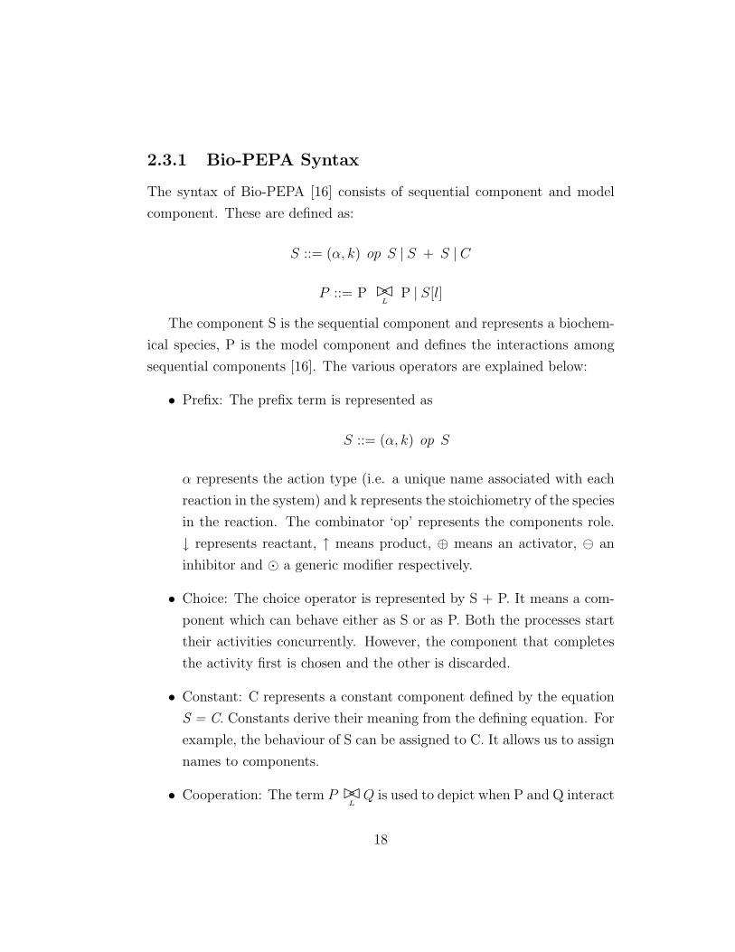
2.3.1 Bio-PEPA Syntax

The syntax of Bio-PEPA [16] consists of sequential component and model

component. These are defined as:

S ::= (α, k) op S | S + S | C

P ::= P ��L

P | S[l]

The component S is the sequential component and represents a biochem-

ical species, P is the model component and defines the interactions among

sequential components [16]. The various operators are explained below:

• Prefix: The prefix term is represented as

S ::= (α, k) op S

α represents the action type (i.e. a unique name associated with each

reaction in the system) and k represents the stoichiometry of the species

in the reaction. The combinator ‘op’ represents the components role.

↓ represents reactant, ↑ means product, ⊕ means an activator, an

inhibitor and � a generic modifier respectively.

• Choice: The choice operator is represented by S + P. It means a com-

ponent which can behave either as S or as P. Both the processes start

their activities concurrently. However, the component that completes

the activity first is chosen and the other is discarded.

• Constant: C represents a constant component defined by the equation

S = C. Constants derive their meaning from the defining equation. For

example, the behaviour of S can be assigned to C. It allows us to assign

names to components.

• Cooperation: The term P ��LQ is used to depict when P and Q interact

18

with each other to carry out an activity together. The common activ-

ities are listed in set L of activities. If an activity is listed in this set,

then the components are forced to synchronise on that activity. The

activities outside set L proceed independently. Note that Bio-PEPA

supports multiway synchronisation, wherein more than 2 components

can cooperate on a given activity.

• Levels of concentration: The term S[l] denotes the number of levels of

each species, where l is the discrete levels of concentration.

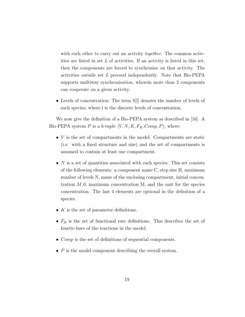
We now give the definition of a Bio-PEPA system as described in [16]. A

Bio-PEPA system P is a 6-tuple 〈V,N,K, FR, Comp, P 〉, where:

• V is the set of compartments in the model. Compartments are static

(i.e. with a fixed structure and size) and the set of compartments is

assumed to contain at least one compartment.

• N is a set of quantities associated with each species. This set consists

of the following elements: a component name C, step size H, maximum

number of levels N, name of the enclosing compartment, initial concen-

tration M 0, maximum concentration M, and the unit for the species

concentration. The last 4 elements are optional in the definition of a

species.

• K is the set of parameter definitions.

• FR is the set of functional rate definitions. This describes the set of

kinetic-laws of the reactions in the model.

• Comp is the set of definitions of sequential components.

• P is the model component describing the overall system.

19

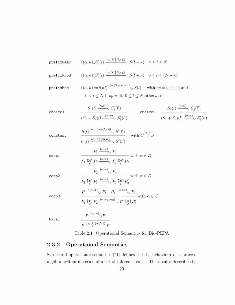
prefixReac ((α, κ)↓S)(l)(α,[S:↓(l,κ)])−−−−−−−−→c S(l − κ) κ ≤ l ≤ N

prefixProd ((α, κ)↑S)(l)(α,[S:↑(l,κ)])−−−−−−−−→c S(l + κ) 0 ≤ l ≤ (N − κ)

prefixMod ((α, κ) op S)(l)(α,[S:op(l,κ)])−−−−−−−−→c S(l) with op = �,⊕, and

0 < l ≤ N if op = ⊕, 0 ≤ l ≤ N otherwise

choice1S1(l)

(α,w)−−−→c S′1(l

′)

(S1 + S2)(l)(α,w)−−−→c S

′1(l

′)choice2

S2(l)(α,w)−−−→c S

′2(l

′)

(S1 + S2)(l)(α,w)−−−→c S

′2(l

′)

constantS(l)

(α,S:[op(l,κ)])−−−−−−−−→c S′(l′)

C(l)(α,C:[op(l,κ)])−−−−−−−−−→c S

′(l′)with C

def= S

coop1P1

(α,w)−−−→c P′1

P1 ��LP2

(α,w)−−−→c P′1��LP2

with α /∈ L

coop2P2

(α,w)−−−→c P′2

P1 ��LP2

(α,w)−−−→c P1 ��LP ′2

with α /∈ L

coop3P1

(α,w1)−−−−→c P′1 P2

(α,w2)−−−−→c P′2

P1 ��LP2

(α,w1::w2)−−−−−−→c P′1��LP ′2

with α ∈ L

FinalP

(αj ,w)−−−−→cP

′

P(αj ,fα(w,N ))7−→ P ′

Table 2.1: Operational Semantics for Bio-PEPA

2.3.2 Operational Semantics

Structural operational semantics [21] defines the the behaviour of a process

algebra system in terms of a set of inference rules. These rules describe the

20

valid transitions of each element in the syntax in terms of the transitions of

its components. The operational semantics for Bio-PEPA systems are given

in Table 2.1 [16]. The first three prefixes define the behaviour of prefix terms

reactant, product and modifier. In case of reactant the level decreases, in

case of product the level increases and in modifiers the level remains the

same. The rules choice 1 and choice 2 define that any one of the two process

can start the activity. The constant rule defines the behaviour of constant

term. The coop1, coop2 and coop3 rules depict the case of co-operation.

The first two rules predict the behaviour when action is enabled and does

not belong to the cooperation set. The rule coopFinal describes the case

in which two components synchronize and information from labels of both

the components are available. The rule Final is included to represent the

rate associated with the transition. The second component fα(w,N) in the

label of the conclusion means that the function fα is evaluated over the list of

quantitative information w and the setN of maximum concentration/number

of levels. The reader is referred to [16] for additional information on the

structural operational semantics of Bio-PEPA.

2.3.3 Example model using Bio-PEPA

We consider the example that we used to illustrate SBML models in Section

2.1.3. To represent this in Bio-PEPA, we define a sequential component for

each species in the model as follows:

• We associate a unique reaction name with each reaction in the system.

• We then define the sequential component for each species. If a species

participates in a reaction, it performs an activity which is the reaction

name. The stoichiometry and role of the species in that reaction are

represented with the syntax described in the previous section. If a

species is participating in multiple reactions, then this represented by

different activities (reaction names) combined with the choice operator.

21

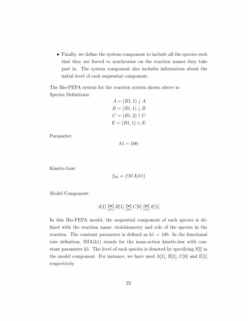
• Finally, we define the system component to include all the species such

that they are forced to synchronise on the reaction names they take

part in. The system component also includes information about the

initial level of each sequential component.

The Bio-PEPA system for the reaction system shown above is:

Species Definitions:

A = (R1, 1) ↓ AB = (R1, 1) ↓ BC = (R1, 2) ↑ CE = (R1, 1)� E

Parameter:

k1 = 100

Kinetic-Law:

fR1 = fMA(k1)

Model Component:

A[1] ��{R1}

B[1] ��{R1}

C[0] ��{R1}

E[1]

In this Bio-PEPA model, the sequential component of each species is de-

fined with the reaction name, stoichiometry and role of the species in the

reaction. The constant parameter is defined as k1 = 100. In the functional

rate definition, fMA(k1) stands for the mass-action kinetic-law with con-

stant parameter k1. The level of each species is denoted by specifying S[l] in

the model component. For instance, we have used A[1], B[1], C[0] and E[1]

respectively.

22

2.4 Software tools

In this section we describe the main software tools we have used in our work.

• Eclipse IDE: We use Eclipse IDE in our work for writing the source

code of the software tool used to convert models from SBML to Bio-

PEPA. Eclipse is a powerful software platform comprised of extensible

application frameworks, tools and runtimes for software development

and management, primarily written in Java and an open-source Inte-

grated Development Environment (IDE) [28]. It has a lot of features

supporting effective Java development such as incremental Java com-

pilation, advanced editing and highlighting of code and syntax errors

and the ability to install various plugins for additional features.

• Bio-PEPA Plug-in: The modelling of the Bio-PEPA models created by

our software tool was done in the Bio-PEPA Eclipse plug-in. It accepts

Bio-PEPA files as input and allows us to run deterministic as well as

stochastic simulations of the Bio-PEPA model. We have considered

the latest available version of the tool. The tool supports deterministic

and stochastic simulations and the implementation of other kinds of

analysis is under development.

• COPASI: COmplex PAthway SImulator (COPASI) [29] is a widely-used

software tool for simulation and analysis of biochemical networks. We

have used COPASI to import and perform simulations of the SBML

models of the pathways we have considered in this thesis. This allows us

to compare the simulation results obtained from the tool and therefore

to validate our translation.

23

2.5 Related Work

There have been some previous works concerned with mapping SBML to

process algebras such as:

• SBML to π-calculus (Bio-SPI tool) [32]

• SBML to stochastic π-calculus (SBML2Pi tool) [33]

• SBML to Beta-binders [18]

Each of the above mappings varies in the level of information that is present

in the translated model. They also differ in the assumptions and the methods

that they follow.

All the above mappings have some limitations. First, only reactions with or-

der up to two can be specified. Indeed, in both pi-calculus and beta-binders,

reactions are abstracted by communications between processes representing

species, and communications are pairwise. Secondly, as a consequence of the

first point, stoichiometric coefficients cannot be represented. Third, these

process algebras assume that the kinetic-law must be of kind mass-action,

whereas rate-laws other than mass-action are common in biological systems.

Finally, analysis by using Gillespie’s algorithms [31] for stochastic simulation

is generally possible but further analysis using different approaches is not.

Note that that both pi-calculus and Beta-binders have been recently extended

with biological transactions in order to handle multiple-reactant multiple-

product reactions [34] [35], but these extensions have not been implemented

in the analysis tools yet, and in the case of the pi-calculus this extension is

not considered in the mapping. We also point out that BlenX [10], a lan-

guage used for modelling biological processes, is based on Beta-binders and

support functional rates but in [18] the standard Beta-binders is used.

Bio-PEPA allows us to represent all these aspects of biochemical systems.

24

Indeed it supports multiway synchronisation so it is possible to map any re-

action, including the ones with order greater than two. In addition to this,

Bio-PEPA supports the definition of stoichiometry and the use of functional

rates to express general rate-laws. Bio-PEPA models also support several

kinds of analysis such as ODE-based, stochastic simulations, continuous time

Markov chain based analysis and model checking.

25

Chapter 3

Mapping from SBML to

Bio-PEPA

The final aim of our work is to map biochemical systems described in SBML

into Bio-PEPA. This allows us to study the systems by using the various

kinds of analysis supported by this process algebra. In this chapter, we de-

scribe the basic elements that are required to build a well-formed Bio-PEPA

model. Then, we explain how these building blocks of Bio-PEPA models

can be obtained from the information in the SBML file. We also discuss

the assumptions we have made and the additional information required for

the successful conversion to Bio-PEPA, as well as the elements which cannot

be mapped into Bio-PEPA. The chapter ends with a summary of the main

features of the mapping from SBML to Bio-PEPA.

3.1 Elements of Bio-PEPA model

A well-formed Bio-PEPA model is defined by a set of compartments, a set

of species, a set of parameters, a set of functional rates, species components

and a model component. We briefly describe below the information required

to build each of these elements. The description of each component is as

26

reported in [16].

1. Compartments: A compartment is described by ‘V: v unit’ where ‘V’

is the compartment name, ‘v’ is a positive real number expressing the

compartment size and ‘unit’ (optional) denotes the unit associated with

the compartment size.

2. Species: Species are defined by a name C, number of levels N, step

size H, initial concentration M0, maximum concentration M, the en-

closing compartment name V and the (optional) unit for the species

concentration.

3. Parameters: Each parameter has an associated name and value, and

an optional unit.

4. Functional rates: There is one functional rate associated with each

reaction, which specifies a mathematical formula denoting the rate of

that reaction.

5. Species components: A Bio-PEPA sequential component abstracts a

species in the biochemical system. Each component specifies the reac-

tions which the species participates in, and the stoichiometry and the

role of the species in the reactions.

6. Model component: This is formed by forcing the species components

to cooperate over the reactions they are involved in. The model com-

ponent also includes information about the initial level of each species.

3.2 The Mapping

In this section, we describe how to define each of the Bio-PEPA model ele-

ments listed in Section 3.1 from the information in the SBML file. Further-

more we discuss the assumptions and limitations of our approach.

27

3.2.1 Compartments

1. SBML files contain a section called ListOfCompartments. Each com-

partment in this list is directly mapped to a compartment in Bio-PEPA.

SBML compartments have a unique ‘ID’ attribute. This ID is mapped

to the compartment name (‘V’) in Bio-PEPA. SBML compartments

also have an optional attribute called ‘size’. This is mapped to the

compartment size (‘v’) in BioPEPA. If the size is not specified in the

SBML file, we set a default size of 1 in the Bio-PEPA model. If a unit

attribute is specified in the SBML model, we map this to the unit in

Bio-PEPA. However, the unit is optional in Bio-PEPA as well, so we

do not specify any default value if it is not present in the SBML file.

2. Strictly speaking, list of compartments is optional in SBML. If there

are no compartments specified, then we add a default compartment of

size 1 in Bio-PEPA. However, if the SBML file defines any species, then

it also has to define at least one compartment since each species must

belong to a compartment in SBML. Hence for all models in practice

SBML files have at least one compartment.

3. The Bio-PEPA Eclipse plugin version we considered does not allow us

to define a compartment whose id is ‘compartment’, although this is

valid in SBML. If we find a SBML compartment with name ‘compart-

ment’ we simply rename it to ‘compartment biopepa’.

4. We give examples to explain the above points. Consider a SBML file

which contains a ListOfCompartments as below:

<ListOfCompartments>

<compartment id = "A" size = "1" units = "volumeUnits" />

<compartment id = "B" size = "2" />

<compartment id = "C" />

</ListOfCompartments>

28

These compartments are converted to Bio-PEPA as below.

compartment A : 1 volumeUnits

compartment B : 2

compartment C : 1

Here, for compartment A the SBML model has all the required infor-

mation. For compartment B, the units are not listed but these are

optional in both SBML and Bio-PEPA so we do not specify any de-

fault. For compartment C, we assume a default size of 1 (the units

depend on the particular model).

3.2.2 Species

1. SBML files contain a section called ListOfSpecies. Each species in this

list is mapped to a species in Bio-PEPA. The SBML definition of species

may include attributes for ID, initialConcentration, compartment and

unit. These attributes are mapped in Bio-PEPA to the species name

‘C’, the initial concentration ‘M0’, the enclosing compartment name

‘V’ and the ‘unit’ for the species concentration respectively.

2. If the initialConcentration is not specified in the SBML file, then it

must be obtained from external sources and inserted in the Bio-PEPA

model. ‘Units’ are optional attributes in both SBML and Bio-PEPA. If

units are not specified in the SBML file, we do not specify any default

value in the Bio-PEPA model.

3. The information about the number of levels ‘N’, the step size ‘H’ and the

maximum concentration ‘M’ cannot be obtained from the SBML file.

We specify a default value of 1 for the step size ‘H’ and 2 for the number

of levels ‘N’ in the Bio-PEPA model. The maximum concentration is

optional in Bio-PEPA, so we do not specify any default value for it. The

29

‘correct’ values for these elements need to be obtained from external

references if they are required for modelling. Note that the values for

these elements are not required if we only want to run ODE-based or

stochastic simulations. They are needed only for CTMC-based analysis

and model checking.

4. The version of the Bio-PEPA Eclipse plugin we considered does not

allow us to use names such as ‘M’, ‘H’, ‘M0’ etc which are used for

defining the properties of species. If we find a species with such a

name, we simply append ‘ species’ to the name.

5. We now give a simple example to explain the above points. Consider

a SBML file which has the following ListOfSpecies:

<listOfSpecies>

<species id = "S1" compartment="A"

initialConcentration = "1" units = "concUnits" />

<species id = "S2" compartment="B" />

</listOfSpecies>

These species are converted to Bio-PEPA as below.

species S1 : M0 = 1, V = A,H = 1, N = 2, unit = concUnits

species S2 : V = B,H = 1, N = 2

3.2.3 Parameters

1. SBML files can contain ListOfParameters in two places: one ‘global’

list and another ‘local parameters’ list included within the KineticLaw

element of a reaction. For each parameter in these lists we create a

Bio-PEPA parameter. The ‘ID’ attribute is mapped to the name and

the ‘value’ attribute is mapped to the value of this parameter in the

Bio-PEPA model. The ‘value’ attribute is optional in SBML; if not

30

specified, it must be obtained from external references and inserted

into the Bio-PEPA model.

2. Parameters local to a reaction can share the same name across different

reactions, but can have different values. However in Bio-PEPA we can

have only one parameter with a given name and its value. So, for

local parameters, we append the reaction ID to the parameter name

to differentiate local parameters of different reactions which have the

same name.

3. The ‘units’ of a parameter are optional in both SBML and Bio-PEPA.

So, we do not specify any default unit if it is not specified in the SBML

file.

4. We explain the above with the help of an example.



<listOfParameters>

<parameter id = "k1" value = "100" />

</listOfParameters>



<listOfParameters>


</listOfParameters>



<listOfParameters>


</listOfParameters>

31

These parameters are converted to Bio-PEPA as below.

k1 = 100

k2 R1 = 200

K2 R2 = 300

The parameter k1 is mapped directly to the corresponding Bio-PEPA

parameter. Both reactions R1 and R2 have a local parameter called k2,

we append the reaction name to the parameter to differentiate them.

3.2.4 Functional Rates

1. SBML files contain a ListOfReactions. For each of the reactions in this

list, we create a name called ‘Alpha N’ where N is an integer number

denoting the number of the reaction in the ListOfReactions. We then

associate a rate formula with this reaction name. This is obtained from

a sub-element called KineticLaw of the reaction in the SBML file. It

represents the rate of the associated reaction.

2. The KineticLaw for a reaction in SBML is optional, however there is

no default rate formula we can use if it is not specified. For those

reactions which do not have a KineticLaw specified, the user will have

to obtain the rate formula from external references and insert this in

the Bio-PEPA model.

3. A reaction can also have an attribute called ‘reversible’ which specifies

whether the reaction is reversible or irreversible. If the value of this

attribute is set to true, then we split the reaction into two irreversible

reactions denoting the forward and backward reactions respectively and

proceed as above to generate the functional rate.

4. Note that the Bio-PEPA syntax allows us to use ‘pre-defined’ rate for-

mulas such a fMA, fMM and fH for mass-action, Michaelis-Menten

32

and Hill kinetics respectively. Although the kinetic-law of a reaction in

SBML might be based on one of these kinetics, it is not possible to get

this information from the SBML file. Hence the Bio-PEPA model will

always contain the expanded formula in terms of species and parame-

ters, instead of just the parameter being used in one of the ‘pre-defined’

functions available in Bio-PEPA.

5. Consider a simple example of an SBML file which contains the following

reaction:




<Kineticlaw>

<math xmlns = "http://www.w3.org/1998/Math/MathML

<apply>

<times/>

<ci>k1</ci>

<ci>S1</ci>

<ci>S2</ci>

</apply>

</math>

</KineticLaw>

</Reaction>

The Bio-PEPA functional rate corresponding to this reaction is speci-

fied as below.

kineticLawOfAlpha 1 : k1 ∗ S1 ∗ S2

33

3.2.5 Species Components

1. SBML files contain a ListOfReactions. For each reaction, we create

a name called ‘Alpha N’ where N is an integer number denoting the

number of the reaction in the ListOfReactions (this name is the same

as the one we used for the functional rates in the earlier subsection).

2. We then create a Bio-PEPA sequential component for each species in

the SBML ListOfSpecies. Each reaction in the list of reactions may

contain a ListOfReactants, ListOfProducts and ListOfModifiers. If a

species occurs in the ListOfReactants/Products/Modifiers of a reaction,

then it performs an action whose name is the one associated with that

reaction (‘Alpha N’ from the above point). The species reference in the

three lists also specifies the stoichiometry of the species. Depending

on which list (reactants, products or modifiers) a species occurs, its

role is specified as ↓ (reactant), ↑ (product), and � (generic modifier)

respectively.

3. SBML does not have a way of representing activators or inhibitors.

Both are grouped under the ListOfModifiers. Hence it is not possible

to specify the exact role of a species as ⊕ (activator) or (inhibitor)

based on the information in a SBML file.

4. Again, we explain this with the help of a simple example. Consider a

list of species and reactions in SBML as below.

<listOfSpecies>

<species id = "S1" compartment = "A" initialAmount="1" />



</listOfSpecies>

<listOfReactions>

34


<listOfReactants>

<speciesreference species = "S1" stoichiometry = "2"/>

</listOfReactants>

<listOfProducts>

<speciesreference species = "S2"/>

</listOfProducts>



</Reaction>


<listOfReactants>


</listOfReactants>

<listOfModifiers>


</listOfModifiers>

<listOfProducts>


</listOfProducts>



</Reaction>

</listOfReactions>

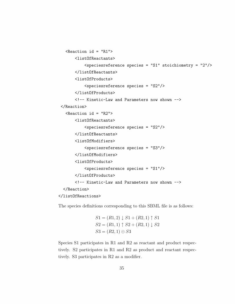
The species definitions corresponding to this SBML file is as follows:

S1 = (R1, 2) ↓ S1 + (R2, 1) ↑ S1

S2 = (R1, 1) ↑ S2 + (R2, 1) ↓ S2

S3 = (R2, 1)� S3

Species S1 participates in R1 and R2 as reactant and product respec-

tively. S2 participates in R1 and R2 as product and reactant respec-

tively. S3 participates in R2 as a modifier.

35

3.2.6 Model Component

1. The model component includes every species in the ListOfSpecies in

the SBML file. Assume that the species in this list are numbered from

1 to N . We include species i in the model component. This is followed

by a list of reactions which species i is forced to synchronise on with

species i + 1 to N . In other words, if a reaction involves species i

and any other species i + 1 to N then the reaction is included in the

synchronisation list listed after species i.

2. Each species should also have an appropriate initial level in the model

component. However, this information cannot be obtained from the

SBML file. We specify a default initial level of 1 for each species in the

model component. The initial level does not matter when we are deal-

ing with ODE-based or stochastic simulation of the Bio-PEPA model.

If a user is interested in performing CTMC based analysis on the model,

he can set the initial level to be the largest integer value which is less

than or equal to M0/H, i.e. the initial concentration divided by the

step size [16].

3. We explain how to build the model component, again considering the

SBML example from Sub-section 3.2.5. Considering the species in or-

der, we first include species S1 with initial level 1. S1 participates in

reaction R1 with S2, and in reaction R2 with both S2 and S3. Hence

both R1 and R2 are included in the synchronisation set listed after S1.

We then list species S2 at initial level 1. S2 participates in reaction R2

with S3. Hence we list R2 in the synchronisation set listed after S2.

We then included the only remaining species S3 in the model defini-

tion, which is then complete. The final model component definition is

as follows:

S1[1] ��{R1,R2}

S2[1] ��{R2}

S3[1]

36

3.3 Limitations of the Mapping

We list below some of the limitations of our mapping from SBML to Bio-

PEPA as described in Section 3.2.

1. The mapping does not consider SBML events. This is because the

Bio-PEPA syntax we have considered does not support the inclusion of

events. However, there has recently been work on incorporating SBML-

like events into Bio-PEPA [36], and in the future we would be able to

include ListOfEvents in our mapping as well.

2. We have ignored the ListOfRules and ListOfInitialAssignments in SBML,

since parameter values and species concentrations in Bio-PEPA are as-

sumed to be initially constant, and not evaluated by functions either

at start or during the course of a model simulation.

3. We are not able to translate certain SBML attributes meaningfully into

Bio-PEPA. For example, we cannot map attributes such as ‘constant =

false’ for SBML compartments, since compartments in Bio-PEPA are

considered to be static. However, an extension of Bio-PEPA to handle

compartments of variable size has recently been defined [37], and this

can be integrated into the mapping in the future.

37

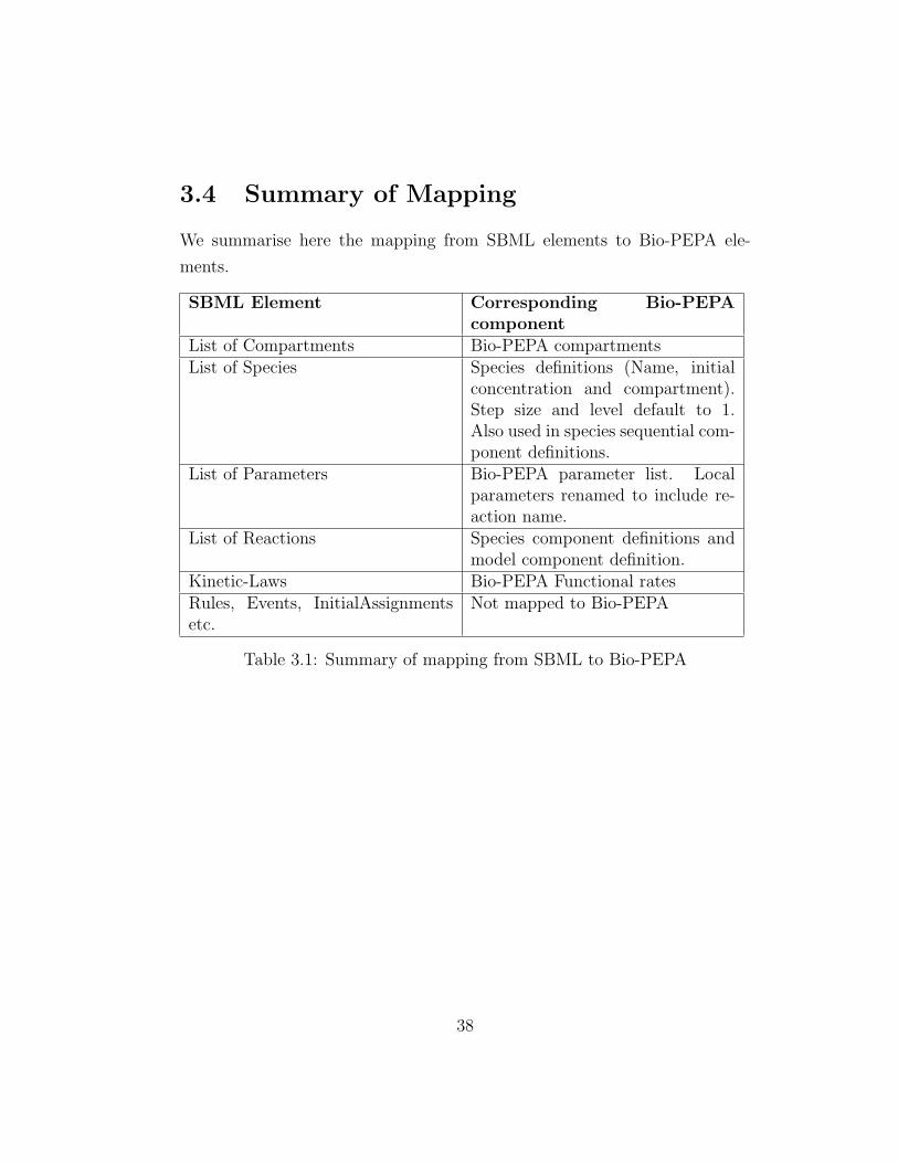
3.4 Summary of Mapping

We summarise here the mapping from SBML elements to Bio-PEPA ele-

ments.

SBML Element Corresponding Bio-PEPAcomponent

List of Compartments Bio-PEPA compartmentsList of Species Species definitions (Name, initial

concentration and compartment).Step size and level default to 1.Also used in species sequential com-ponent definitions.

List of Parameters Bio-PEPA parameter list. Localparameters renamed to include re-action name.

List of Reactions Species component definitions andmodel component definition.

Kinetic-Laws Bio-PEPA Functional ratesRules, Events, InitialAssignmentsetc.

Not mapped to Bio-PEPA

Table 3.1: Summary of mapping from SBML to Bio-PEPA

38

Chapter 4

Software Tool

This chapter is devoted to the description of the tool called ‘SBML2BioPEPA’

which implements the mapping from SBML to Bio-PEPA as discussed in

Chapter 3. We begin by describing the reasons for our choice of development

tools. We then describe the main software classes created for the development

of the tool.

4.1 Development Tools

Our software tool SBML2BioPEPA has been implemented in the JAVA pro-

gramming language [38]. The Eclipse IDE has been used for development.

The reasons for our choices are reported below:

1. The most important reason for this choice of language was to enable

closer integration with other Bio-PEPA tools. The Bio-PEPA plugin

which is used for modelling and simulation of Bio-PEPA models is

written entirely in Java (based on the Eclipse IDE). Using the same

language for the development of our tool means that the two could be

easily integrated in the future.

2. Another important reason is that there are several third-party tools

39

written for programming in Java which ease the development process.

We would like to particularly mention the availability of a Java Appli-

cation Programming Interface (API) for processing SBML files called

libSBML [39]. This has been embedded in our tool to allow us to easily

read SBML models.

3. Java is a modern object-oriented programming language. It allows us

to build individual parts of our tool (using standalone Java classes) and

then bring them together to compose the whole tool. This speeds up

the development process considerably.

4. Finally, Java is a highly portable language which can run on a wide

variety of platforms. This allows us to easily deploy our tool in different

environments.

4.2 Java Classes Design

We now explain some of the main classes used in the software tool. Figure 4.1

gives an overview of the main classes of our software. Note that this figure

does not show the internal details of the classes. These will be explained

along with the corresponding class description below.

1. SBML2BioPEPA: This is the main class of the application. It rep-

resents the class which does the actual mapping from a SBML file to

a Bio-PEPA file suitable for use in the Bio-PEPA Eclipse plugin. This

class does not have any data members. It only accepts from the user

the SBML file which is to be converted to Bio-PEPA, and the name

of the file in which to write the Bio-PEPA model. Internally, the class

uses the SBMLModel and BioPEPAModel classes (described below)

for storing the model data. We briefly explain below some of the main

methods of this class.

40

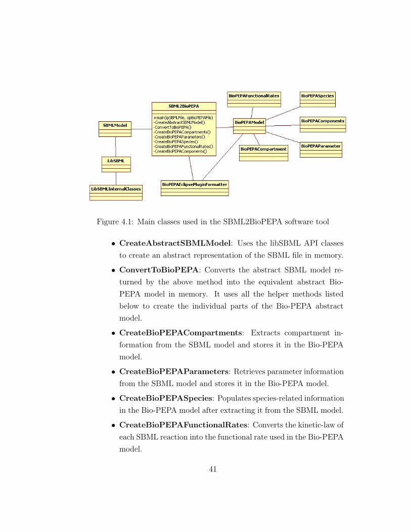
Figure 4.1: Main classes used in the SBML2BioPEPA software tool

• CreateAbstractSBMLModel: Uses the libSBML API classes

to create an abstract representation of the SBML file in memory.

• ConvertToBioPEPA: Converts the abstract SBML model re-

turned by the above method into the equivalent abstract Bio-

PEPA model in memory. It uses all the helper methods listed

below to create the individual parts of the Bio-PEPA abstract

model.

• CreateBioPEPACompartments: Extracts compartment in-

formation from the SBML model and stores it in the Bio-PEPA

model.

• CreateBioPEPAParameters: Retrieves parameter information

from the SBML model and stores it in the Bio-PEPA model.

• CreateBioPEPASpecies: Populates species-related information

in the Bio-PEPA model after extracting it from the SBML model.

• CreateBioPEPAFunctionalRates: Converts the kinetic-law of

each SBML reaction into the functional rate used in the Bio-PEPA

model.

41

• CreateBioPEPAComponents: Using the information about

reactions (such as participating species and their stoichiometries),

creates the species sequential Bio-PEPA components as well as the

overall model component and stores this in the abstract Bio-PEPA

model in memory.

2. SBMLModel: This class represents the abstract model of the SBML

file. Internally it uses the libSBML API and its data structures to hold

information about the SBML model in memory.

3. LibSBML and LibSBMLInternal classes: These classes are the

API wrappers provided by libSBML to manipulate SBML documents.

They are used to parse the SBML file and to create a in-memory rep-

resentation of the corresponding SBML model.

4. BioPEPEEclipsePluginFormatter: This class is used to create a

Bio-PEPA file suitable for use in the Bio-PEPA Eclipse plugin. This

class queries the BioPEPAModel for information about the model, and

then writes this to a Bio-PEPA file.

5. BioPEPAModel: Represents the Bio-PEPA model in an abstract

manner in memory, i.e. it contains all those details which can be used to

create a well-formed Bio-PEPA model. Internally, this class uses several

container classes (listed below) to store all the information about the

Bio-PEPA model.

6. BioPEPACompartment: Contains all the information required to

represent a compartment in Bio-PEPA, namely it has data members

for the name, size and unit of size.

7. BioPEPASpecies: This class represents a Bio-PEPA species. It is

able to hold information about the species name, enclosing compart-

ment, initial and maximum concentrations, concentration units, step

size and number of levels.

42

8. BioPEPAParameter: Represents information about a parameter in

Bio-PEPA, i.e. parameter name, value and unit.

9. BioPEPAFunctionalRate: Contains data members to represent in-

formation associated with functional rates such as the reaction name

and the mathematical formula for the rate of the reaction.

10. BioPEPAComponent: There is one instance of this class associated

with each species, which represents the Bio-PEPA sequential compo-

nent. It contains an array of data members to represent the reactions

this species is involved in, and the role and stoichiometry of the species

in each reaction.

4.3 Tool Deployment

In this section, we describe how the tool we have created is used in practice.

We also describe how to deploy it on different operating system platforms.

• The output of the Java classes we have written is a SBML2BioPEPA.JAR

file. This file contains the Java executable code which performs the

mapping.

• In addition, we also have a libSBML.JAR file which contains the exe-

cutable code for the libSBML API.

• To be able to use our tool, the user should copy both of these files into

a single folder. Then the user should issue the following command:

java -jar SBML2BioPEPA.jar <InputSBMLFile> <OutputBioPEPAFile>

• Here, InputSBMLFile represents the SBML file we want to convert to

Bio-PEPA. OutputBioPEPAFile represents the filename in which we

want the translated model to be stored.

43

• The output Bio-PEPA file uses the same syntax for representing Bio-

PEPA models as the Bio-PEPA Eclipse Plugin; this syntax is described

in Appendix C.

• The tool prints out status information such as which elements were suc-

cessfully mapped, and if there were any problems during the mapping.

44

Chapter 5

Case Studies

In this chapter, we discuss the modelling and simulation of two biochemi-

cal networks, namely the Synthetic Oscillatory Network model (also called

the Repressilator) [40] and the Mitogen Activated Protein Kinase (MAPK)

pathway [42]. The SBML models of these biological pathways are obtained

from the BioModels model repository [23] and converted to Bio-PEPA using

our tool. We begin the chapter by describing each of the biological mod-

els in detail. Then, we show how the components in the SBML models are

translated into Bio-PEPA using the software tool described in the previous

chapter. Finally, the results obtained by simulating the Bio-PEPA models in

the Bio-PEPA Eclipse plugin are explained and compared with the results

reported in the literature and the results obtained by simulation in COPASI

with the same SBML file.

45

5.1 Repressilator - A Synthetic Oscillatory

Network

5.1.1 Description of the model

The Repressilator is a synthetic regulatory gene network composed of three

genes whose protein products mutually suppress each other. This synthetic

network was implemented in E. coli [40].

The model consists of three proteins Lacl from E. coli, TetR from the

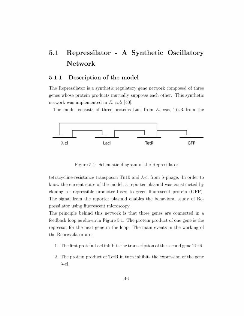
Figure 5.1: Schematic diagram of the Represillator

tetracycline-resistance transposon Tn10 and λ-cl from λ-phage. In order to

know the current state of the model, a reporter plasmid was constructed by

cloning tet-repressible promoter fused to green fluorescent protein (GFP).

The signal from the reporter plasmid enables the behavioral study of Re-

pressilator using fluorescent microscopy.

The principle behind this network is that three genes are connected in a

feedback loop as shown in Figure 5.1. The protein product of one gene is the

repressor for the next gene in the loop. The main events in the working of

the Repressilator are:

1. The first protein Lacl inhibits the transcription of the second gene TetR.

2. The protein product of TetR in turn inhibits the expression of the gene

λ-cl.

46

3. Finally, λ-cl protein inhibits Lacl expression thus completing the cycle.

As each gene represses the next gene in the loop, this results in cyclic tem-

poral oscillations in the concentrations of the three proteins in the network.

Each of the three proteins participates in the different transcription, transla-

tion and degradation reactions in various roles. The authors of [40] suggest

that the temporal oscillations are due to the variation in the concentrations

of each of its components.

5.1.2 Mapping Description

The SBML model for the Repressilator was downloaded from the BioMod-

els database (BioModels number BIOMD0000000012). Using the tool we

implemented, we were successfully able to convert this SBML file into the

corresponding Bio-PEPA model. In this section, we describe the components

in the SBML file and how they are translated into components of the Bio-

PEPA model. The syntax for the Bio-PEPA model is the one used in the

Bio-PEPA Eclipse plugin as described in Appendix C.

The SBML model file for the Repressilator consists of the following elements:

1. One compartment ‘cell’ of size 1.

2. 6 species as listed in Table 5.1. The species X, Y and Z are the tran-

scripts of mRNA and they express proteins PX, PY and PZ respec-

tively. All the species are located in the compartment ‘cell’. The SBML

file reports the initial amounts of each species; these values are reported

in Table 5.1.

47

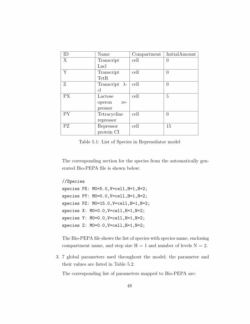
ID Name Compartment InitialAmountX Transcript

Laclcell 0

Y TranscriptTetR

cell 0

Z Transcript λ-cl

cell 0

PX Lactoseoperon re-pressor

cell 5

PY Tetracyclinerepressor

cell 0

PZ Repressorprotein CI

cell 15

Table 5.1: List of Species in Repressilator model

The corresponding section for the species from the automatically gen-

erated Bio-PEPA file is shown below:

//Species

species PX: M0=5.0,V=cell,H=1,N=2;

species PY: M0=0.0,V=cell,H=1,N=2;

species PZ: M0=15.0,V=cell,H=1,N=2;

species X: M0=0.0,V=cell,H=1,N=2;

species Y: M0=0.0,V=cell,H=1,N=2;

species Z: M0=0.0,V=cell,H=1,N=2;

The Bio-PEPA file shows the list of species with species name, enclosing

compartment name, and step size H = 1 and number of levels N = 2.

3. 7 global parameters used throughout the model; the parameter and

their values are listed in Table 5.2.

The corresponding list of parameters mapped to Bio-PEPA are:

48

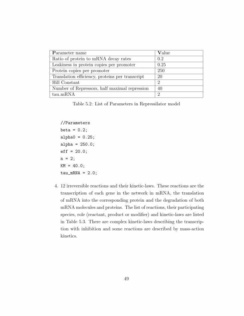
Parameter name ValueRatio of protein to mRNA decay rates 0.2Leakiness in protein copies per promoter 0.25Protein copies per promoter 250Translation efficiency, proteins per transcript 20Hill Constant 2Number of Repressors, half maximal repression 40tau mRNA 2

Table 5.2: List of Parameters in Repressilator model

//Parameters

beta = 0.2;

alpha0 = 0.25;

alpha = 250.0;

eff = 20.0;

n = 2;

KM = 40.0;

tau_mRNA = 2.0;

4. 12 irreversible reactions and their kinetic-laws. These reactions are the

transcription of each gene in the network in mRNA, the translation

of mRNA into the corresponding protein and the degradation of both

mRNA molecules and proteins. The list of reactions, their participating

species, role (reactant, product or modifier) and kinetic-laws are listed

in Table 5.3. There are complex kinetic-laws describing the transcrip-

tion with inhibition and some reactions are described by mass-action

kinetics.

49

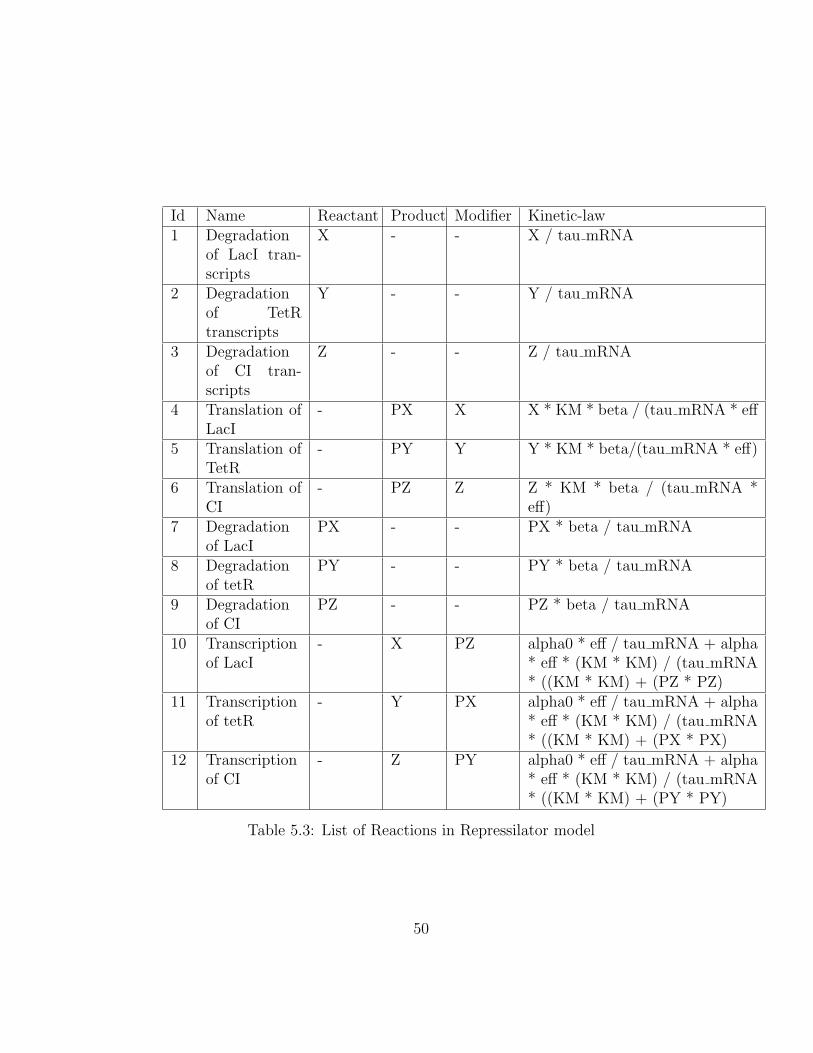
Id Name Reactant Product Modifier Kinetic-law1 Degradation

of LacI tran-scripts

X - - X / tau mRNA

2 Degradationof TetRtranscripts

Y - - Y / tau mRNA

3 Degradationof CI tran-scripts

Z - - Z / tau mRNA

4 Translation ofLacI

- PX X X * KM * beta / (tau mRNA * eff

5 Translation ofTetR

- PY Y Y * KM * beta/(tau mRNA * eff)

6 Translation ofCI

- PZ Z Z * KM * beta / (tau mRNA *eff)

7 Degradationof LacI

PX - - PX * beta / tau mRNA

8 Degradationof tetR

PY - - PY * beta / tau mRNA

9 Degradationof CI

PZ - - PZ * beta / tau mRNA

10 Transcriptionof LacI

- X PZ alpha0 * eff / tau mRNA + alpha* eff * (KM * KM) / (tau mRNA* ((KM * KM) + (PZ * PZ)

11 Transcriptionof tetR

- Y PX alpha0 * eff / tau mRNA + alpha* eff * (KM * KM) / (tau mRNA* ((KM * KM) + (PX * PX)

12 Transcriptionof CI

- Z PY alpha0 * eff / tau mRNA + alpha* eff * (KM * KM) / (tau mRNA* ((KM * KM) + (PY * PY)

Table 5.3: List of Reactions in Repressilator model

50

The kinetic-law of each reaction is mapped to the corresponding func-

tional rate in Bio-PEPA.

//Functional Rates

kineticLawOf Alpha_0 : X / tau_mRNA;

kineticLawOf Alpha_1 : Y / tau_mRNA;

kineticLawOf Alpha_2 : Z / tau_mRNA;

kineticLawOf Alpha_3 : X * KM * beta / (tau_mRNA * eff);

kineticLawOf Alpha_4 : Y * KM * beta / (tau_mRNA * eff);

kineticLawOf Alpha_5 : Z * KM * beta / (tau_mRNA * eff);

kineticLawOf Alpha_6 : PX * beta / tau_mRNA;

kineticLawOf Alpha_7 : PY * beta / tau_mRNA;

kineticLawOf Alpha_8 : PZ * beta / tau_mRNA;

kineticLawOf Alpha_9 : alpha0 * eff / tau_mRNA + alpha * eff *

(KM * KM) / (tau_mRNA * ((KM * KM) + (PZ * PZ)));


(KM * KM) / (tau_mRNA * ((KM * KM) + (PX * PX)));


(KM * KM) / (tau_mRNA * ((KM * KM) + (PY * PY)));

The information about reactions in the SBML file is used to create

the sequential components and the model component in Bio-PEPA as

described in Chapter 3. The species definitions and the complete model

component in the obtained Bio-PEPA file are listed below:

//Components

PX = (Alpha_3,1.0) >> PX

+ (Alpha_6,1.0) << PX

+ (Alpha_10,1.0) (.) PX;

X = (Alpha_0,1.0) << X

+ (Alpha_3,1.0) (.) X

51

+ (Alpha_9,1.0) >> X;

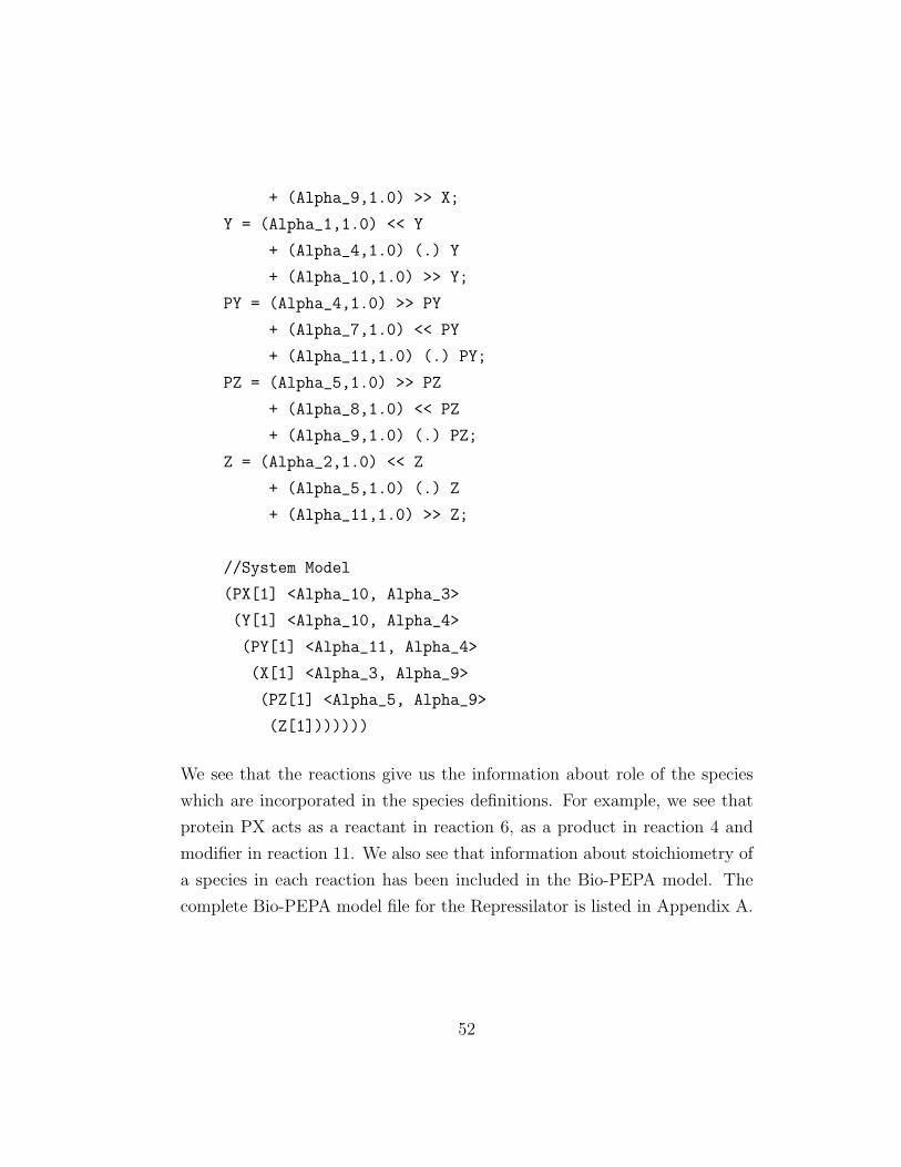
Y = (Alpha_1,1.0) << Y

+ (Alpha_4,1.0) (.) Y

+ (Alpha_10,1.0) >> Y;

PY = (Alpha_4,1.0) >> PY

+ (Alpha_7,1.0) << PY

+ (Alpha_11,1.0) (.) PY;

PZ = (Alpha_5,1.0) >> PZ

+ (Alpha_8,1.0) << PZ

+ (Alpha_9,1.0) (.) PZ;

Z = (Alpha_2,1.0) << Z

+ (Alpha_5,1.0) (.) Z

+ (Alpha_11,1.0) >> Z;

//System Model

(PX[1] <Alpha_10, Alpha_3>

(Y[1] <Alpha_10, Alpha_4>

(PY[1] <Alpha_11, Alpha_4>

(X[1] <Alpha_3, Alpha_9>

(PZ[1] <Alpha_5, Alpha_9>

(Z[1]))))))

We see that the reactions give us the information about role of the species

which are incorporated in the species definitions. For example, we see that

protein PX acts as a reactant in reaction 6, as a product in reaction 4 and

modifier in reaction 11. We also see that information about stoichiometry of

a species in each reaction has been included in the Bio-PEPA model. The

complete Bio-PEPA model file for the Repressilator is listed in Appendix A.

52

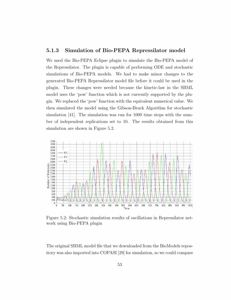
5.1.3 Simulation of Bio-PEPA Repressilator model

We used the Bio-PEPA Eclipse plugin to simulate the Bio-PEPA model of

the Repressilator. The plugin is capable of performing ODE and stochastic

simulations of Bio-PEPA models. We had to make minor changes to the

generated Bio-PEPA Repressilator model file before it could be used in the

plugin. These changes were needed because the kinetic-law in the SBML

model uses the ‘pow’ function which is not currently supported by the plu-

gin. We replaced the ‘pow’ function with the equivalent numerical value. We

then simulated the model using the Gibson-Bruck Algorithm for stochastic

simulation [41]. The simulation was run for 1000 time steps with the num-

ber of independent replications set to 10. The results obtained from this

simulation are shown in Figure 5.2.

Figure 5.2: Stochastic simulation results of oscillations in Repressilator net-work using Bio-PEPA plugin

The original SBML model file that we downloaded from the BioModels repos-

itory was also imported into COPASI [29] for simulation, so we could compare

53

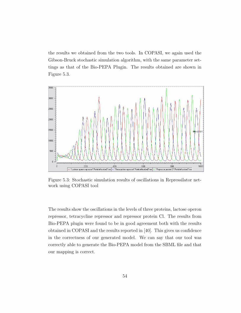
the results we obtained from the two tools. In COPASI, we again used the

Gibson-Bruck stochastic simulation algorithm, with the same parameter set-

tings as that of the Bio-PEPA Plugin. The results obtained are shown in

Figure 5.3.

Figure 5.3: Stochastic simulation results of oscillations in Repressilator net-work using COPASI tool

The results show the oscillations in the levels of three proteins, lactose operon

repressor, tetracycline repressor and repressor protein Cl. The results from

Bio-PEPA plugin were found to be in good agreement both with the results

obtained in COPASI and the results reported in [40]. This gives us confidence

in the correctness of our generated model. We can say that our tool was

correctly able to generate the Bio-PEPA model from the SBML file and that

our mapping is correct.

54

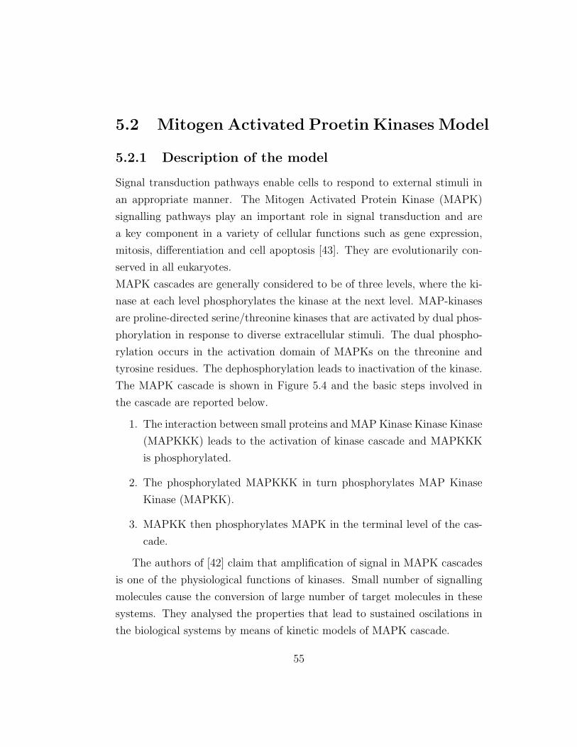
5.2 Mitogen Activated Proetin Kinases Model

5.2.1 Description of the model

Signal transduction pathways enable cells to respond to external stimuli in

an appropriate manner. The Mitogen Activated Protein Kinase (MAPK)

signalling pathways play an important role in signal transduction and are

a key component in a variety of cellular functions such as gene expression,

mitosis, differentiation and cell apoptosis [43]. They are evolutionarily con-

served in all eukaryotes.

MAPK cascades are generally considered to be of three levels, where the ki-

nase at each level phosphorylates the kinase at the next level. MAP-kinases

are proline-directed serine/threonine kinases that are activated by dual phos-

phorylation in response to diverse extracellular stimuli. The dual phospho-

rylation occurs in the activation domain of MAPKs on the threonine and

tyrosine residues. The dephosphorylation leads to inactivation of the kinase.

The MAPK cascade is shown in Figure 5.4 and the basic steps involved in

the cascade are reported below.

1. The interaction between small proteins and MAP Kinase Kinase Kinase

(MAPKKK) leads to the activation of kinase cascade and MAPKKK

is phosphorylated.

2. The phosphorylated MAPKKK in turn phosphorylates MAP Kinase

Kinase (MAPKK).

3. MAPKK then phosphorylates MAPK in the terminal level of the cas-

cade.

The authors of [42] claim that amplification of signal in MAPK cascades

is one of the physiological functions of kinases. Small number of signalling

molecules cause the conversion of large number of target molecules in these

systems. They analysed the properties that lead to sustained oscilations in

the biological systems by means of kinetic models of MAPK cascade.

55

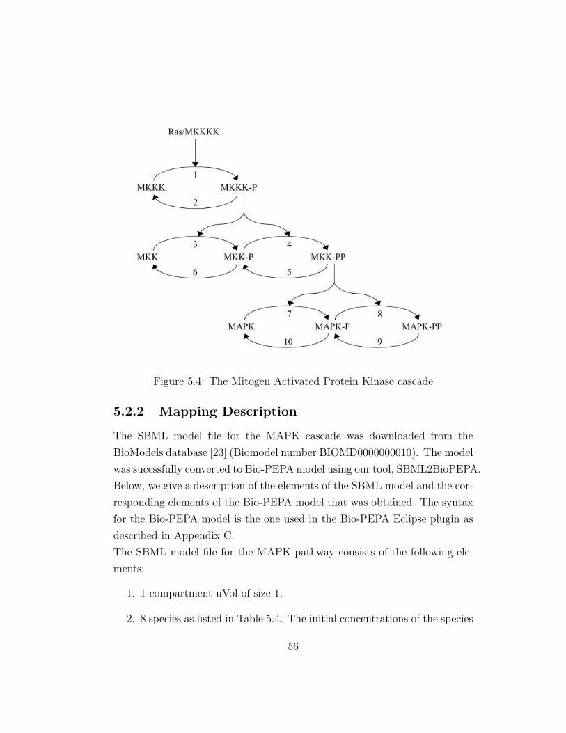
Figure 5.4: The Mitogen Activated Protein Kinase cascade

5.2.2 Mapping Description

The SBML model file for the MAPK cascade was downloaded from the

BioModels database [23] (Biomodel number BIOMD0000000010). The model

was sucessfully converted to Bio-PEPA model using our tool, SBML2BioPEPA.

Below, we give a description of the elements of the SBML model and the cor-

responding elements of the Bio-PEPA model that was obtained. The syntax

for the Bio-PEPA model is the one used in the Bio-PEPA Eclipse plugin as

described in Appendix C.

The SBML model file for the MAPK pathway consists of the following ele-

ments:

1. 1 compartment uVol of size 1.

2. 8 species as listed in Table 5.4. The initial concentrations of the species

56

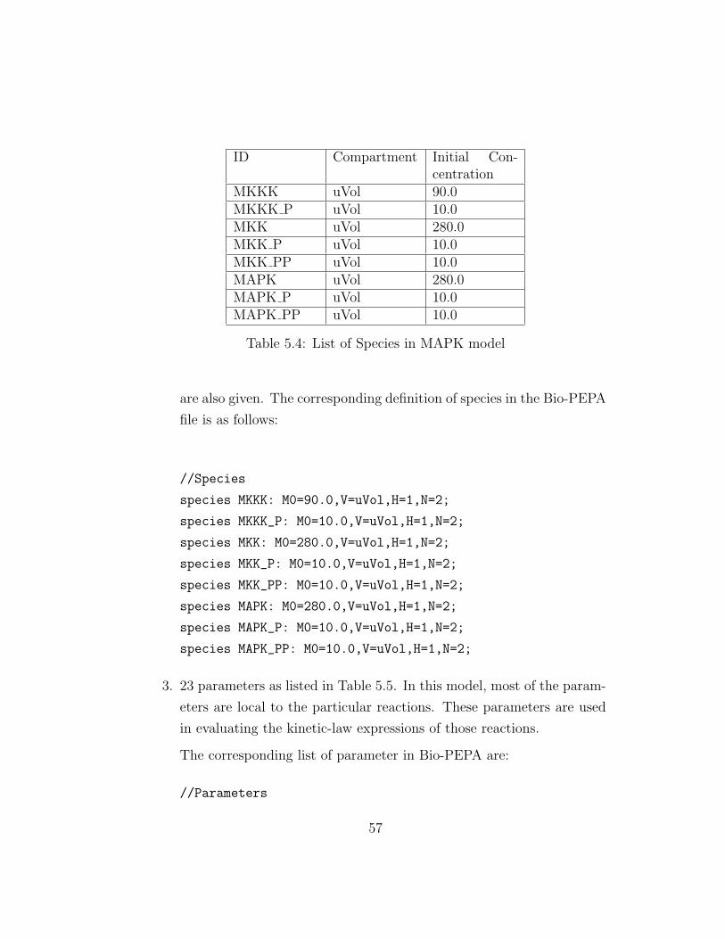
ID Compartment Initial Con-centration

MKKK uVol 90.0MKKK P uVol 10.0MKK uVol 280.0MKK P uVol 10.0MKK PP uVol 10.0MAPK uVol 280.0MAPK P uVol 10.0MAPK PP uVol 10.0

Table 5.4: List of Species in MAPK model

are also given. The corresponding definition of species in the Bio-PEPA

file is as follows:

//Species

species MKKK: M0=90.0,V=uVol,H=1,N=2;

species MKKK_P: M0=10.0,V=uVol,H=1,N=2;

species MKK: M0=280.0,V=uVol,H=1,N=2;

species MKK_P: M0=10.0,V=uVol,H=1,N=2;

species MKK_PP: M0=10.0,V=uVol,H=1,N=2;

species MAPK: M0=280.0,V=uVol,H=1,N=2;

species MAPK_P: M0=10.0,V=uVol,H=1,N=2;

species MAPK_PP: M0=10.0,V=uVol,H=1,N=2;

3. 23 parameters as listed in Table 5.5. In this model, most of the param-

eters are local to the particular reactions. These parameters are used

in evaluating the kinetic-law expressions of those reactions.

The corresponding list of parameter in Bio-PEPA are:

//Parameters

57

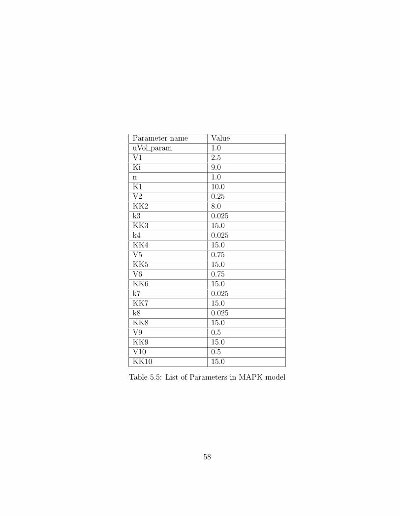
Parameter name ValueuVol param 1.0V1 2.5Ki 9.0n 1.0K1 10.0V2 0.25KK2 8.0k3 0.025KK3 15.0k4 0.025KK4 15.0V5 0.75KK5 15.0V6 0.75KK6 15.0k7 0.025KK7 15.0k8 0.025KK8 15.0V9 0.5KK9 15.0V10 0.5KK10 15.0

Table 5.5: List of Parameters in MAPK model

58

uVol_param = 1.0;

V1 = 2.5;

Ki = 9.0;

K1 = 10.0;

V2 = 0.25;

KK2 = 8.0;

k3 = 0.025;

KK3 = 15.0;

k4 = 0.025;

KK4 = 15.0;

V5 = 0.75;

KK5 = 15.0;

V6 = 0.75;

KK6 = 15.0;

k7 = 0.025;

KK7 = 15.0;

k8 = 0.025;

KK8 = 15.0;

V9 = 0.5;

KK9 = 15.0;

V10 = 0.5;

KK10 = 15.0;

4. 12 Reactions as listed in Table 5.6. The table also lists the reactants,

products and modifiers along with the kinetic-laws of the reactions.

The kinases with dual specificity follow the Michaelis-Menten rate-

law [42]. Therefore, the rate equations in the cascade are shown by

Michaelis-Menten kinetics. The catalytic rate constants and maximal

enzymatic rates for each reaction are given in the list of parameters.

The functional rates corresponding to the kinetic-laws are expressed in

the Bio-PEPA file as shown:

59

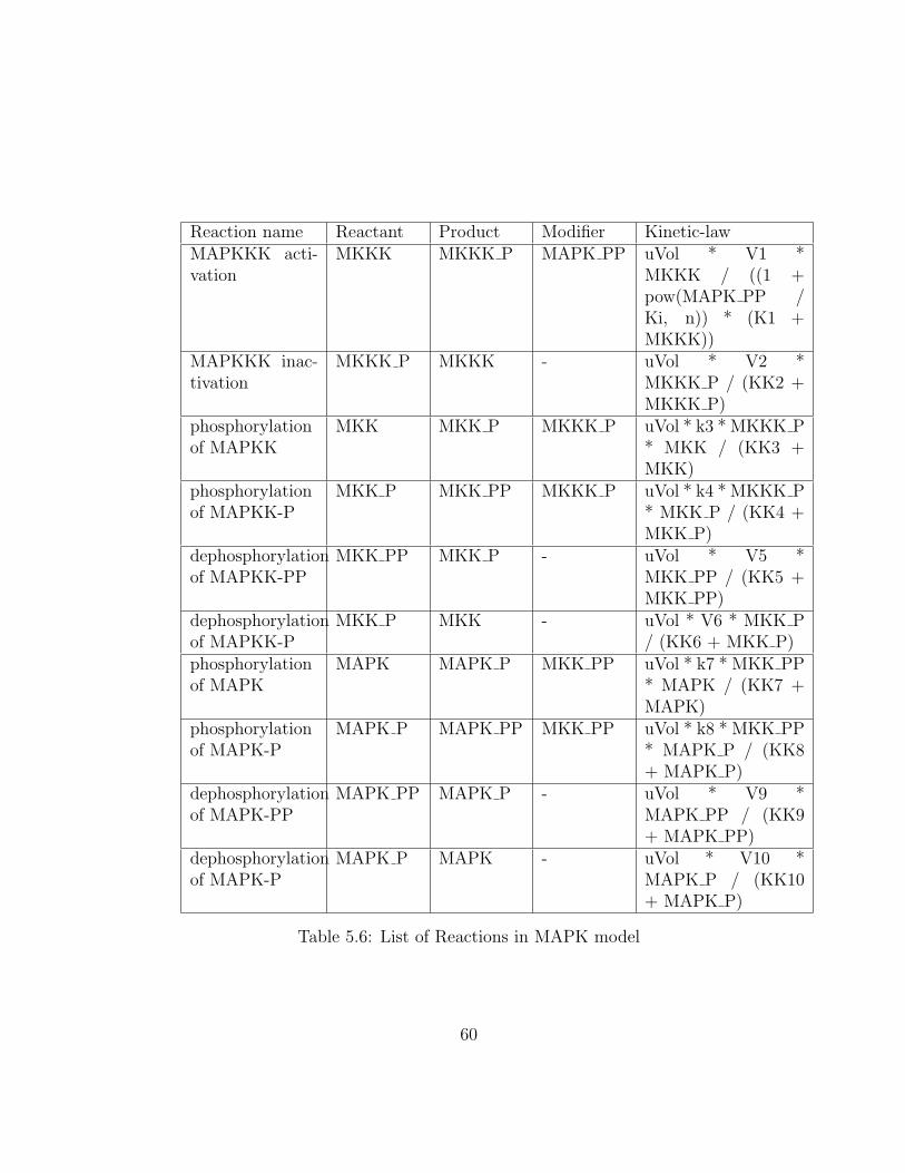
Reaction name Reactant Product Modifier Kinetic-lawMAPKKK acti-vation

MKKK MKKK P MAPK PP uVol * V1 *MKKK / ((1 +pow(MAPK PP /Ki, n)) * (K1 +MKKK))

MAPKKK inac-tivation

MKKK P MKKK - uVol * V2 *MKKK P / (KK2 +MKKK P)

phosphorylationof MAPKK

MKK MKK P MKKK P uVol * k3 * MKKK P* MKK / (KK3 +MKK)

phosphorylationof MAPKK-P

MKK P MKK PP MKKK P uVol * k4 * MKKK P* MKK P / (KK4 +MKK P)

dephosphorylationof MAPKK-PP

MKK PP MKK P - uVol * V5 *MKK PP / (KK5 +MKK PP)

dephosphorylationof MAPKK-P

MKK P MKK - uVol * V6 * MKK P/ (KK6 + MKK P)

phosphorylationof MAPK

MAPK MAPK P MKK PP uVol * k7 * MKK PP* MAPK / (KK7 +MAPK)

phosphorylationof MAPK-P

MAPK P MAPK PP MKK PP uVol * k8 * MKK PP* MAPK P / (KK8+ MAPK P)

dephosphorylationof MAPK-PP

MAPK PP MAPK P - uVol * V9 *MAPK PP / (KK9+ MAPK PP)

dephosphorylationof MAPK-P

MAPK P MAPK - uVol * V10 *MAPK P / (KK10+ MAPK P)

Table 5.6: List of Reactions in MAPK model

60

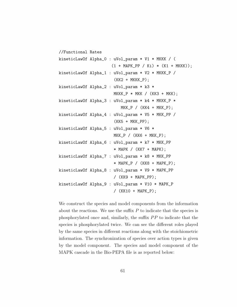
//Functional Rates

kineticLawOf Alpha_0 : uVol_param * V1 * MKKK / (

(1 + MAPK_PP / Ki) * (K1 + MKKK));

kineticLawOf Alpha_1 : uVol_param * V2 * MKKK_P /

(KK2 + MKKK_P);

kineticLawOf Alpha_2 : uVol_param * k3 *

MKKK_P * MKK / (KK3 + MKK);

kineticLawOf Alpha_3 : uVol_param * k4 * MKKK_P *

MKK_P / (KK4 + MKK_P);

kineticLawOf Alpha_4 : uVol_param * V5 * MKK_PP /

(KK5 + MKK_PP);

kineticLawOf Alpha_5 : uVol_param * V6 *


kineticLawOf Alpha_6 : uVol_param * k7 * MKK_PP

* MAPK / (KK7 + MAPK);

kineticLawOf Alpha_7 : uVol_param * k8 * MKK_PP

* MAPK_P / (KK8 + MAPK_P);

kineticLawOf Alpha_8 : uVol_param * V9 * MAPK_PP

/ (KK9 + MAPK_PP);

kineticLawOf Alpha_9 : uVol_param * V10 * MAPK_P

/ (KK10 + MAPK_P);

We construct the species and model components from the information

about the reactions. We use the suffix P to indicate that the species is

phosphorylated once and, similarly, the suffix PP to indicate that the

species is phosphorylated twice. We can see the different roles played

by the same species in different reactions along with the stoichiometric

information. The synchronization of species over action types is given

by the model component. The species and model component of the

MAPK cascade in the Bio-PEPA file is as reported below:

61

//Components

MAPK = (Alpha_6,1.0) << MAPK +

(Alpha_9,1.0) >> MAPK;

MKK_P = (Alpha_2,1.0) >> MKK_P +

(Alpha_3,1.0) << MKK_P +

(Alpha_4,1.0) >> MKK_P +

(Alpha_5,1.0) << MKK_P;

MKK_PP = (Alpha_3,1.0) >> MKK_PP +

(Alpha_4,1.0) << MKK_PP +

(Alpha_6,1.0) (.) MKK_PP +

(Alpha_7,1.0) (.) MKK_PP;

MKKK_P = (Alpha_0,1.0) >> MKKK_P +

(Alpha_1,1.0) << MKKK_P +

(Alpha_2,1.0) (.) MKKK_P +

(Alpha_3,1.0) (.) MKKK_P;

MKK = (Alpha_2,1.0) << MKK +

(Alpha_5,1.0) >> MKK;

MAPK_PP = (Alpha_0,1.0) (.) MAPK_PP +

(Alpha_7,1.0) >> MAPK_PP +

(Alpha_8,1.0) << MAPK_PP;

MAPK_P = (Alpha_6,1.0) >> MAPK_P +

(Alpha_7,1.0) << MAPK_P +

(Alpha_8,1.0) >> MAPK_P +

(Alpha_9,1.0) << MAPK_P;

MKKK = (Alpha_0,1.0) << MKKK + (Alpha_1,1.0) >> MKKK;

//System Model

(MAPK[1] <Alpha_6, Alpha_9>

(MKK_P[1] <Alpha_2, Alpha_3, Alpha_4, Alpha_5>

(MKK_PP[1] <Alpha_3, Alpha_4, Alpha_6, Alpha_7>

62

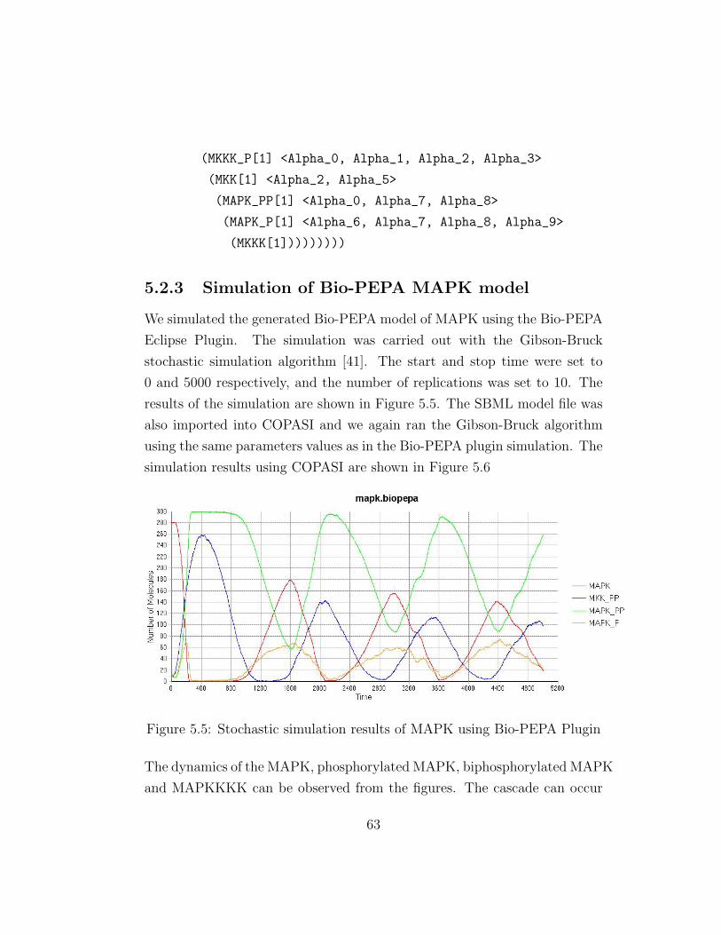
(MKKK_P[1] <Alpha_0, Alpha_1, Alpha_2, Alpha_3>

(MKK[1] <Alpha_2, Alpha_5>

(MAPK_PP[1] <Alpha_0, Alpha_7, Alpha_8>

(MAPK_P[1] <Alpha_6, Alpha_7, Alpha_8, Alpha_9>

(MKKK[1]))))))))

5.2.3 Simulation of Bio-PEPA MAPK model

We simulated the generated Bio-PEPA model of MAPK using the Bio-PEPA

Eclipse Plugin. The simulation was carried out with the Gibson-Bruck

stochastic simulation algorithm [41]. The start and stop time were set to

0 and 5000 respectively, and the number of replications was set to 10. The

results of the simulation are shown in Figure 5.5. The SBML model file was

also imported into COPASI and we again ran the Gibson-Bruck algorithm

using the same parameters values as in the Bio-PEPA plugin simulation. The

simulation results using COPASI are shown in Figure 5.6

Figure 5.5: Stochastic simulation results of MAPK using Bio-PEPA Plugin

The dynamics of the MAPK, phosphorylated MAPK, biphosphorylated MAPK

and MAPKKKK can be observed from the figures. The cascade can occur

63

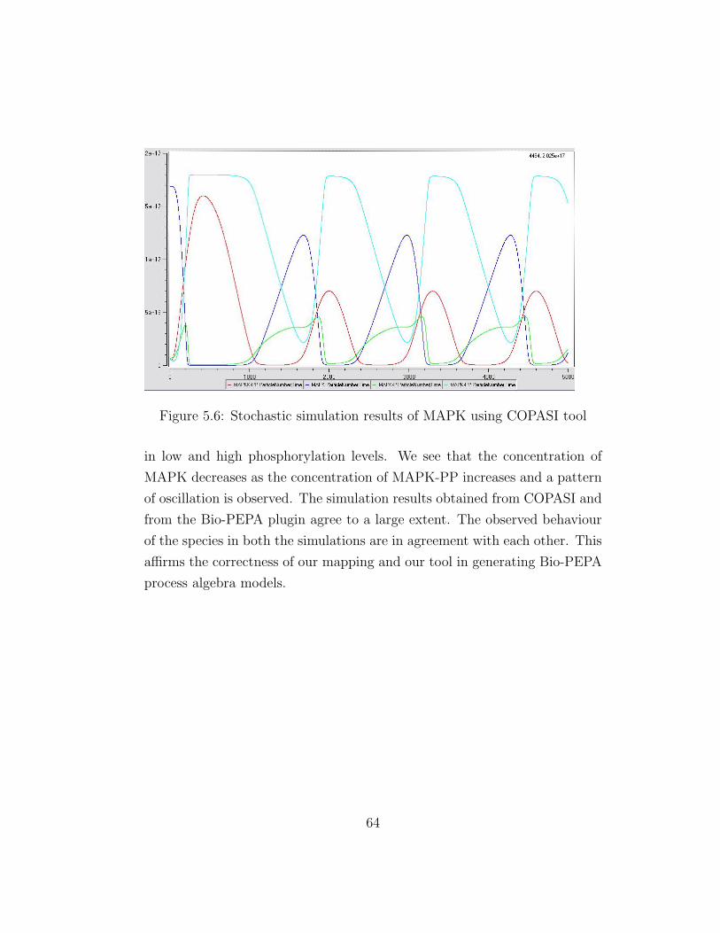
Figure 5.6: Stochastic simulation results of MAPK using COPASI tool

in low and high phosphorylation levels. We see that the concentration of

MAPK decreases as the concentration of MAPK-PP increases and a pattern

of oscillation is observed. The simulation results obtained from COPASI and

from the Bio-PEPA plugin agree to a large extent. The observed behaviour

of the species in both the simulations are in agreement with each other. This

affirms the correctness of our mapping and our tool in generating Bio-PEPA

process algebra models.

64

Chapter 6

Conclusions

In this chapter we summarise the outcome of our thesis. In Section 6.1 we

give some concluding remarks about our work. Section 6.2 presents possible

future enhancements to the mapping and tool that we have developed.

6.1 Concluding remarks

This thesis concentrated on developing a translation from SBML to Bio-

PEPA. First, we formalised the theoretical mapping of elements between the

two languages: we defined the building blocks of SBML and Bio-PEPA and

proposed the translation rules. Then, we mentioned some assumptions and

limitations of our mapping. After that, we presented SBML2BioPEPA, the

JAVA-based software tool we developed to implement this mapping. The

Bio-PEPA models produced by this tool were suitable for use in the Bio-

PEPA Eclipse plugin. Finally, we tested and validated our mapping and

software tool using two sample SBML models from the BioModels database.

The first model we chose was the Repressilator model. We downloaded the

SBML model and translated it into the equivalent Bio-PEPA model using

our software tool. Stochastic simulations of the model were performed us-

ing the Bio-PEPA Eclipse plugin, and another set of simulation results were

65

obtained by importing the same SBML file into COPASI. The simulation re-

sults obtained from both the tools were in good agreement with each other.

The second model we considered was the MAPK pathway. Again, we per-

formed the translation from the SBML file for the MAPK model to Bio-

PEPA. Stochastic simulations of this model were then performed using both

the Bio-PEPA plugin and COPASI. The results from both tools were very

similar to each other. The agreement between the results obtained for both

the models prove the correctness of our mapping and software tool as we

were able to reproduce the results as reported in the literature.

As we considered the Bio-PEPA formalism in our work, it was possible to

translate reactions of order more than two in a straight-forward way as op-

posed to other process algebras which only support reactions upto order of

two (note that that both pi-calculus and Beta-binders have been recently

extended with biological transactions in order to handle multiple-reactant

multiple-product reactions [34] [35], but these extensions have not been im-

plemented in the analysis tools yet). Another advantage of using Bio-PEPA

was that kinetic-laws other than mass-action could be easily specified. This

was possible because Bio-PEPA has the concept of functional rates which al-

lows us to express general kinetic-laws. Stoichiometric information of species

could also be specified in Bio-PEPA. Our work was highly motivated by all

these advantages that Bio-PEPA offers over other process algebras.

6.2 Further Work

There are several possible future directions for the work we have described

in this thesis. We report some of them below:

1. Translation of models from Bio-PEPA to SBML - An auto-

matic tool for the reverse translation from Bio-PEPA to SBML models

would be very useful. Bio-PEPA models could then be exchanged and

communicated between various research groups within the scientific

66

community.

2. Extension of the software tool - The software tool we have devel-

oped could be extended by creating a friendly graphical user interface

(GUI). Such a GUI could enable the user to interact more in the transla-

tion process. For example, users could enter missing parameter values,

or an integrated interface to external references could be provided for

gathering information related to the model.

3. Integration with Bio-PEPA Eclipse plugin - The software tool

that we have developed could be integrated with the Bio-PEPA Eclipse

plugin. This would present a single platform for users to be able to

create and work with Bio-PEPA models.

4. Translation involving SBML events - In the translation proposed

in this thesis, we do not consider the list of events from the SBML

file. Recently, SBML-like events have been added to the Bio-PEPA

syntax [36]. An improvement of our work could be to include the

events definition in the mapping and the software tool.

5. Supporting variable SBML compartment sizes - In the present

work, one of the assumptions of our translation is that the sizes of

compartments are static with constant volumes. Recently, the Bio-

PEPA syntax has been enhanced to include variable compartment sizes

[37]. The concept of variable compartment sizes could be included in

the mapping in the future.

67

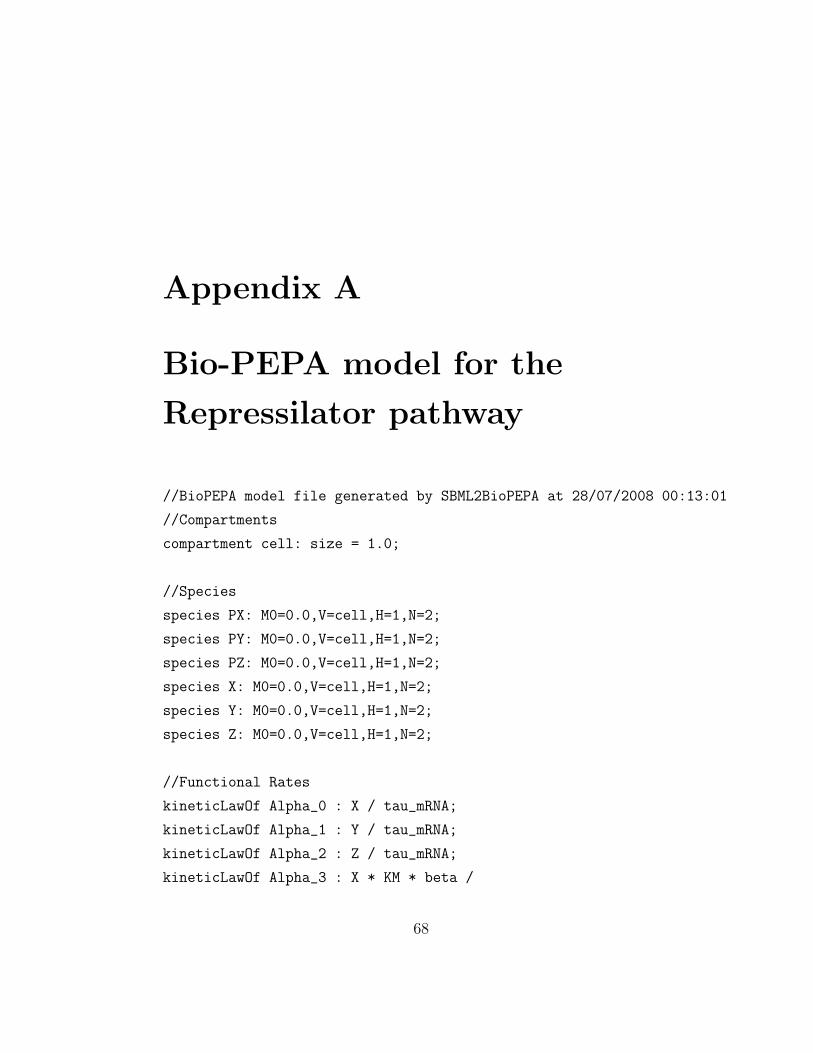
Appendix A

Bio-PEPA model for the

Repressilator pathway

//BioPEPA model file generated by SBML2BioPEPA at 28/07/2008 00:13:01

//Compartments

compartment cell: size = 1.0;

//Species

species PX: M0=0.0,V=cell,H=1,N=2;

species PY: M0=0.0,V=cell,H=1,N=2;

species PZ: M0=0.0,V=cell,H=1,N=2;

species X: M0=0.0,V=cell,H=1,N=2;

species Y: M0=0.0,V=cell,H=1,N=2;

species Z: M0=0.0,V=cell,H=1,N=2;

//Functional Rates

kineticLawOf Alpha_0 : X / tau_mRNA;

kineticLawOf Alpha_1 : Y / tau_mRNA;

kineticLawOf Alpha_2 : Z / tau_mRNA;

kineticLawOf Alpha_3 : X * KM * beta /

68

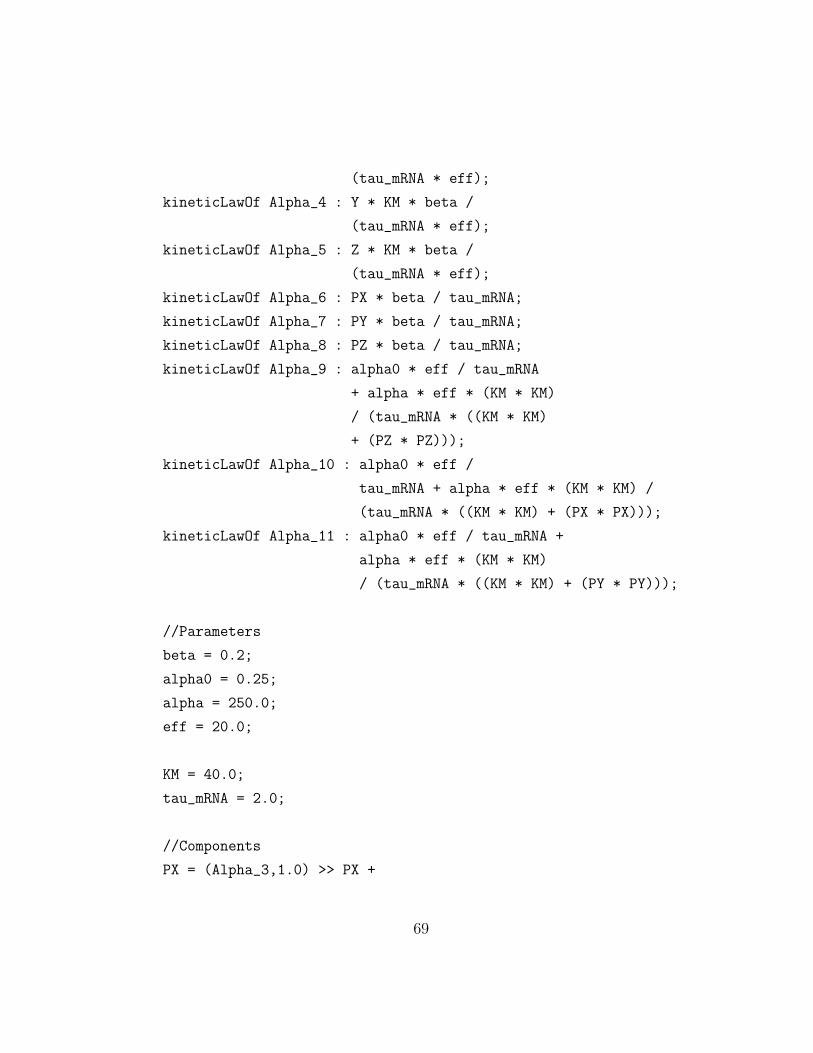
(tau_mRNA * eff);

kineticLawOf Alpha_4 : Y * KM * beta /

(tau_mRNA * eff);

kineticLawOf Alpha_5 : Z * KM * beta /

(tau_mRNA * eff);

kineticLawOf Alpha_6 : PX * beta / tau_mRNA;

kineticLawOf Alpha_7 : PY * beta / tau_mRNA;

kineticLawOf Alpha_8 : PZ * beta / tau_mRNA;

kineticLawOf Alpha_9 : alpha0 * eff / tau_mRNA

+ alpha * eff * (KM * KM)

/ (tau_mRNA * ((KM * KM)

+ (PZ * PZ)));

kineticLawOf Alpha_10 : alpha0 * eff /

tau_mRNA + alpha * eff * (KM * KM) /

(tau_mRNA * ((KM * KM) + (PX * PX)));

kineticLawOf Alpha_11 : alpha0 * eff / tau_mRNA +

alpha * eff * (KM * KM)

/ (tau_mRNA * ((KM * KM) + (PY * PY)));

//Parameters

beta = 0.2;

alpha0 = 0.25;

alpha = 250.0;

eff = 20.0;

KM = 40.0;

tau_mRNA = 2.0;

//Components

PX = (Alpha_3,1.0) >> PX +

69

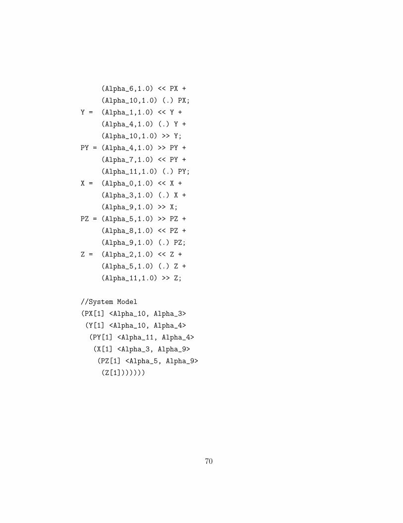
(Alpha_6,1.0) << PX +

(Alpha_10,1.0) (.) PX;

Y = (Alpha_1,1.0) << Y +

(Alpha_4,1.0) (.) Y +

(Alpha_10,1.0) >> Y;

PY = (Alpha_4,1.0) >> PY +

(Alpha_7,1.0) << PY +

(Alpha_11,1.0) (.) PY;

X = (Alpha_0,1.0) << X +

(Alpha_3,1.0) (.) X +

(Alpha_9,1.0) >> X;

PZ = (Alpha_5,1.0) >> PZ +

(Alpha_8,1.0) << PZ +

(Alpha_9,1.0) (.) PZ;

Z = (Alpha_2,1.0) << Z +

(Alpha_5,1.0) (.) Z +

(Alpha_11,1.0) >> Z;

//System Model

(PX[1] <Alpha_10, Alpha_3>

(Y[1] <Alpha_10, Alpha_4>

(PY[1] <Alpha_11, Alpha_4>

(X[1] <Alpha_3, Alpha_9>

(PZ[1] <Alpha_5, Alpha_9>

(Z[1]))))))

70

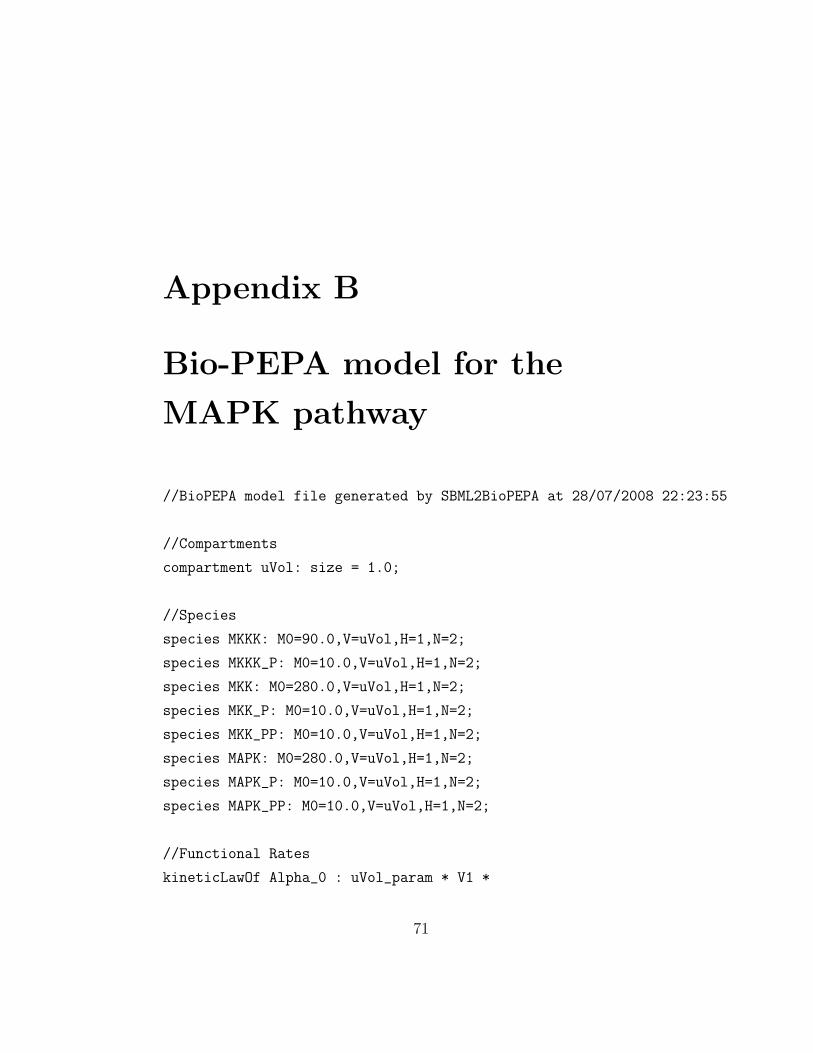
Appendix B

Bio-PEPA model for the

MAPK pathway

//BioPEPA model file generated by SBML2BioPEPA at 28/07/2008 22:23:55

//Compartments

compartment uVol: size = 1.0;

//Species


species MKKK_P: M0=10.0,V=uVol,H=1,N=2;

species MKK: M0=280.0,V=uVol,H=1,N=2;

species MKK_P: M0=10.0,V=uVol,H=1,N=2;

species MKK_PP: M0=10.0,V=uVol,H=1,N=2;

species MAPK: M0=280.0,V=uVol,H=1,N=2;

species MAPK_P: M0=10.0,V=uVol,H=1,N=2;

species MAPK_PP: M0=10.0,V=uVol,H=1,N=2;

//Functional Rates


71

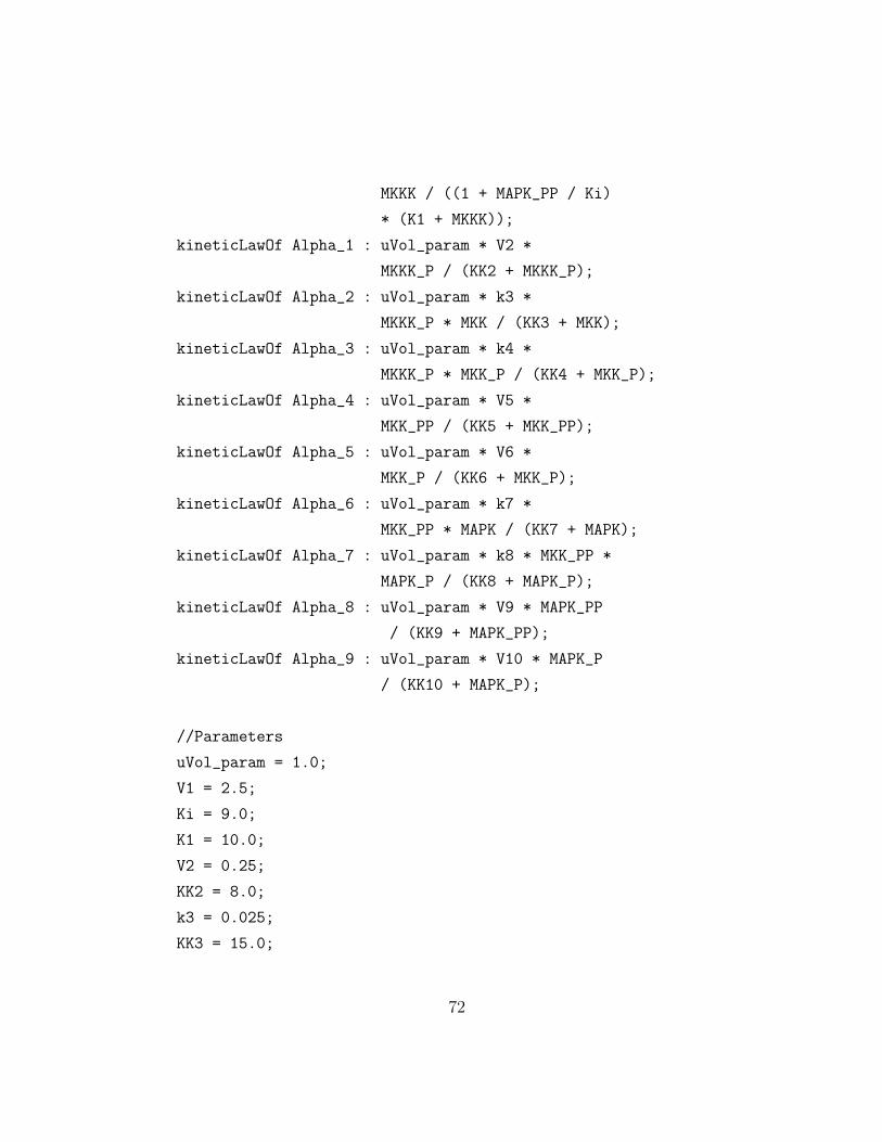
MKKK / ((1 + MAPK_PP / Ki)

* (K1 + MKKK));


MKKK_P / (KK2 + MKKK_P);


MKKK_P * MKK / (KK3 + MKK);


MKKK_P * MKK_P / (KK4 + MKK_P);


MKK_PP / (KK5 + MKK_PP);




MKK_PP * MAPK / (KK7 + MAPK);

kineticLawOf Alpha_7 : uVol_param * k8 * MKK_PP *

MAPK_P / (KK8 + MAPK_P);

kineticLawOf Alpha_8 : uVol_param * V9 * MAPK_PP

/ (KK9 + MAPK_PP);

kineticLawOf Alpha_9 : uVol_param * V10 * MAPK_P

/ (KK10 + MAPK_P);

//Parameters

uVol_param = 1.0;

V1 = 2.5;

Ki = 9.0;

K1 = 10.0;

V2 = 0.25;

KK2 = 8.0;

k3 = 0.025;

KK3 = 15.0;

72

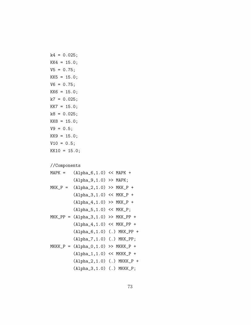
k4 = 0.025;

KK4 = 15.0;

V5 = 0.75;

KK5 = 15.0;

V6 = 0.75;

KK6 = 15.0;

k7 = 0.025;

KK7 = 15.0;

k8 = 0.025;

KK8 = 15.0;

V9 = 0.5;

KK9 = 15.0;

V10 = 0.5;

KK10 = 15.0;

//Components

MAPK = (Alpha_6,1.0) << MAPK +

(Alpha_9,1.0) >> MAPK;

MKK_P = (Alpha_2,1.0) >> MKK_P +

(Alpha_3,1.0) << MKK_P +

(Alpha_4,1.0) >> MKK_P +

(Alpha_5,1.0) << MKK_P;



(Alpha_6,1.0) (.) MKK_PP +


MKKK_P = (Alpha_0,1.0) >> MKKK_P +

(Alpha_1,1.0) << MKKK_P +

(Alpha_2,1.0) (.) MKKK_P +

(Alpha_3,1.0) (.) MKKK_P;

73

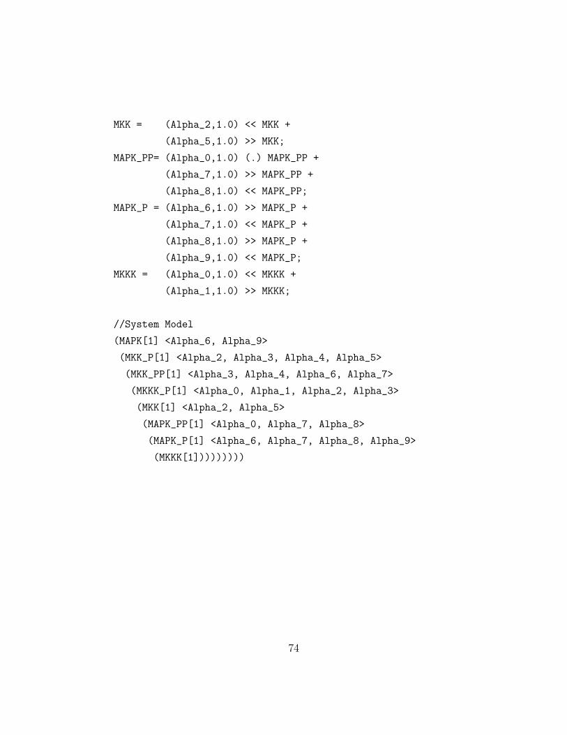
MKK = (Alpha_2,1.0) << MKK +

(Alpha_5,1.0) >> MKK;

MAPK_PP= (Alpha_0,1.0) (.) MAPK_PP +

(Alpha_7,1.0) >> MAPK_PP +

(Alpha_8,1.0) << MAPK_PP;

MAPK_P = (Alpha_6,1.0) >> MAPK_P +

(Alpha_7,1.0) << MAPK_P +

(Alpha_8,1.0) >> MAPK_P +

(Alpha_9,1.0) << MAPK_P;

MKKK = (Alpha_0,1.0) << MKKK +

(Alpha_1,1.0) >> MKKK;

//System Model








(MKKK[1]))))))))

74

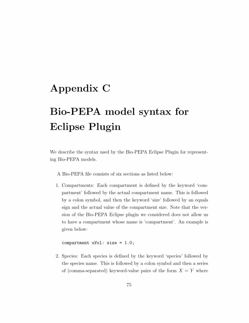
Appendix C

Bio-PEPA model syntax for

Eclipse Plugin

We describe the syntax used by the Bio-PEPA Eclipse Plugin for represent-

ing Bio-PEPA models.

A Bio-PEPA file consists of six sections as listed below:

1. Compartments: Each compartment is defined by the keyword ‘com-

partment’ followed by the actual compartment name. This is followed

by a colon symbol, and then the keyword ‘size’ followed by an equals

sign and the actual value of the compartment size. Note that the ver-

sion of the Bio-PEPA Eclipse plugin we considered does not allow us

to have a compartment whose name is ’compartment’. An example is

given below:

compartment uVol: size = 1.0;

2. Species: Each species is defined by the keyword ‘species’ followed by

the species name. This is followed by a colon symbol and then a series

of (comma-separated) keyword-value pairs of the form X = Y where

75

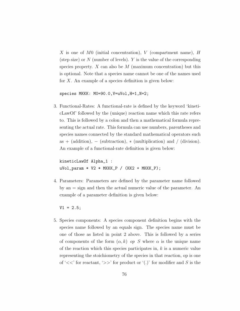
X is one of M0 (initial concentration), V (compartment name), H

(step size) or N (number of levels). Y is the value of the corresponding

species property. X can also be M (maximum concentration) but this

is optional. Note that a species name cannot be one of the names used

for X. An example of a species definition is given below:


3. Functional-Rates: A functional-rate is defined by the keyword ‘kineti-

cLawOf’ followed by the (unique) reaction name which this rate refers

to. This is followed by a colon and then a mathematical formula repre-

senting the actual rate. This formula can use numbers, parentheses and

species names connected by the standard mathematical operators such

as + (addition), − (subtraction), ∗ (multiplication) and / (division).

An example of a functional-rate definition is given below:

kineticLawOf Alpha_1 :

uVol_param * V2 * MKKK_P / (KK2 + MKKK_P);

4. Parameters: Parameters are defined by the parameter name followed

by an = sign and then the actual numeric value of the parameter. An

example of a parameter definition is given below:

V1 = 2.5;

5. Species components: A species component definition begins with the

species name followed by an equals sign. The species name must be

one of those as listed in point 2 above. This is followed by a series

of components of the form (α, k) op S where α is the unique name

of the reaction which this species participates in, k is a numeric value

representing the stoichiometry of the species in that reaction, op is one

of ‘<<’ for reactant, ‘>>’ for product or ‘(.)’ for modifier and S is the

76

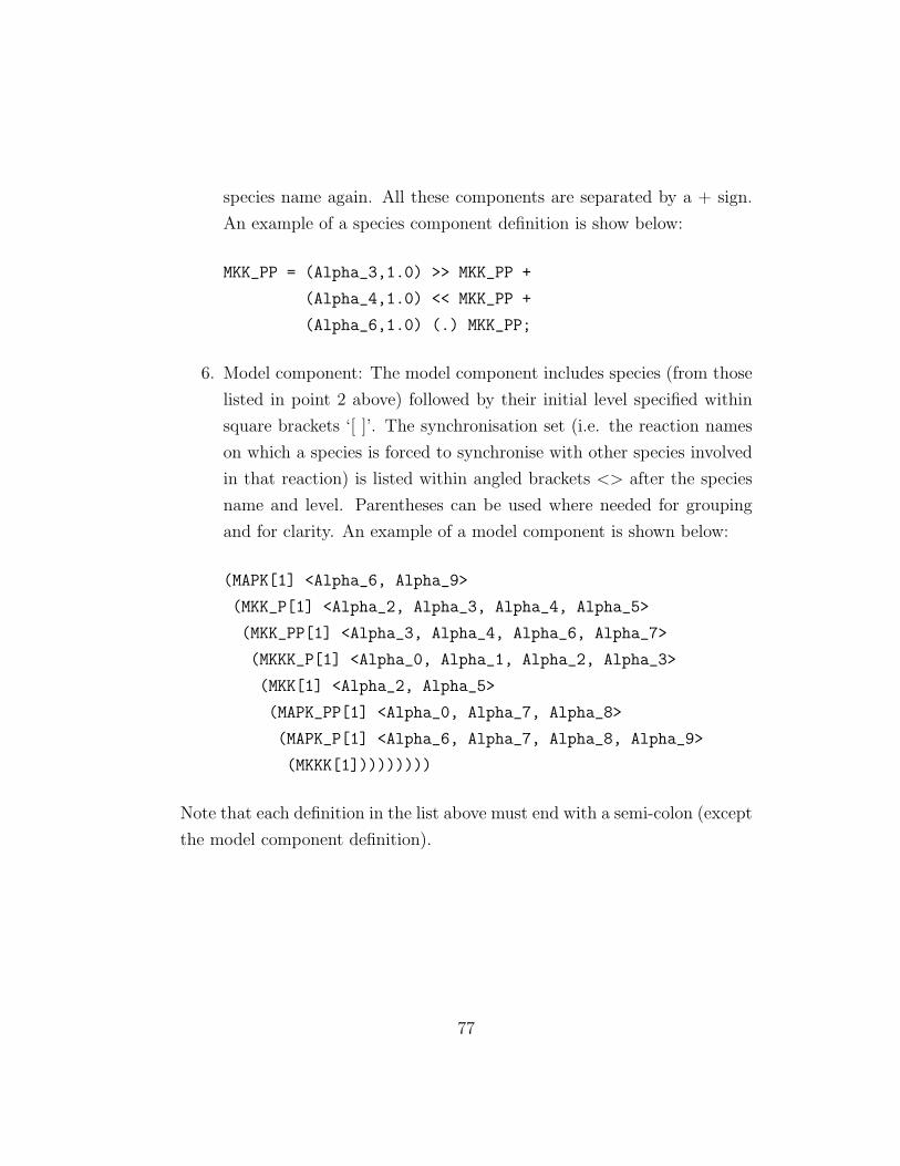
species name again. All these components are separated by a + sign.

An example of a species component definition is show below:




6. Model component: The model component includes species (from those

listed in point 2 above) followed by their initial level specified within

square brackets ‘[ ]’. The synchronisation set (i.e. the reaction names

on which a species is forced to synchronise with other species involved

in that reaction) is listed within angled brackets <> after the species

name and level. Parentheses can be used where needed for grouping

and for clarity. An example of a model component is shown below:








(MKKK[1]))))))))

Note that each definition in the list above must end with a semi-colon (except

the model component definition).

77

Bibliography

[1] H. Kitano. Systems Biology: A Brief Overview. Science, Volume 295,

Pages 1662-1664, 2002.

[2] E. Klipp, R. Herwig, A. Kowald, C. Wierling, H. Lehrach. Systems

Biology in Practice. Wiley-VCH, 2005.

[3] P. Hartman. Theory of Ordinary Differential Equations. Society for In-

dustrial and Applied Mathematics, 2nd edition, 2002.

[4] T. Murata. Petri nets: Properties, Analysis and Applications, Proceed-

ings of the IEEE, Volume 77, Issue 4, Pages 541-580, 1989.

[5] R. Milner. Communicating and Mobile Systems: the π-calculus. Cam-

bridge University Press, 1999.

[6] T. Akutsu et al. Identification of Genetic Networks from a small number

of Gene Expression Patterns under the Boolean Network Model. Pacific

Symposium on Biocomputing, Volume 1, Pages 1728, 1999.

[7] E. Godehardt and O. Richter. Application of Graph Theory in Modelling

of Biological Systems. Proceedings of the First European Simulation

Congress, Volume 71, Pages 580-587, 1987.

[8] C. Priami, A. Regev, W. Silverman and E. Shapiro. Application of a

Stochastic Name Passing Calculus to Representation and Simulation of

78

Molecular Processes. Information Processing Letters, Volume 80, Num-

ber 1, 2001.

[9] P. Degano, D. Prandi, C. Priami and P. Quaglia. Beta-binders for Bio-

logical Quantitative Experiments. Electronic Notes in Theoretical Com-

puter Science, Volume 164, Issue 3, Pages 101-117, 2006.

[10] L. Dematte, C. Priami, A. Romanel. Modelling and Simulation of Bio-

logical Processes in BlenX. SIGMETRICS Performance Evaluation Re-

view, Volume 35, Pages 32-39, 2008.

[11] M. Calder, S. Gilmore, and J. Hillston. Modelling the Influence of RKIP

on the ERK Signalling Pathway using the Stochastic Process Algebra

PEPA. In Anna Ingolfsdottir and Hanne Riis Nielson, editors, Proceed-

ings of the BioConcur Workshop on Concurrent Models in Molecular

Biology, London, England, August 2004.

[12] F. Ciocchetta, J. Hillston. Process Algebras in Systems Biology. For-

mal Methods for Computational Systems Biology. SFM 2008, Advance

Lectures, Springer, Pages 265-312, 2008.

[13] V. Danos and J. Krivine. Formal Molecular Biology Done in CCS-R.

Electronic Notes in Theoretical Computer Science, Volume 180, Pages

31-49, 2007.

[14] L. Bortolussi and A. Policriti. Modelling Biological Systems in Stochastic

Concurrent Constraint Programming. Constraints, Volume 13, Pages 66-

90, 2008.

[15] V. Danos and C. Laneve. Formal molecular biology. Theoretical Com-

puter Science, Volume 325, Pages 69-110, 2004.

[16] F. Ciocchetta and J. Hillston. Bio-PEPA: A Framework for the Mod-

elling and Analysis of Biological Systems. Electronic Notes in Theoreti-

cal Computer Science, Science Direct, Volume 194, Pages 103-117, 2008.

79

[17] J.C.M. Baeten. A Brief History of Process Algebras. Theoretical Com-

puter Science, Volume 335, Issue 2-3, Pages 131-146, 2005.

[18] F. Ciocchetta, C. Priami and P. Quaglia. An Automatic Translation of

SBML into Beta-Binders. IEEE/ACM Transactions on computational

Biology and Bioinformatics. IEEE Computer Society Digital Library,

Volume 5, Pages 80-90, 2008.

[19] C. Priami. Stochastic π-Calculus. The Computer Journal, Volume 38,

Number 6, Pages 578-589, 1995.

[20] J. Hillston. A Compositional Approach to Performance Modelling. Cam-

bridge University Press, 1996.

[21] G. Plotkin. A Structural Approach to Operational Semantics. Technical

report, DAIMI FN-19, Aarhus University, Denmark, 1981.

[22] M. Hucka, A. Finney, B.J. Bornstein, S.M. Keating, B.E. Shapiro, J.

Matthews, B.L. Kovitz, M.J. Schilstra, A. Funahashi, J.C. Doyle and H.

Kitano. Evolving a Lingua Franca and Associated Software Infrastruc-

ture for Computational Systems Biology: The Systems Biology Markup

Language (SBML) Project, Systems Biology, Volume 1, Pages 41-53,

2004.

[23] http://www.ebi.ac.uk/biomodels/

[24] http://www.w3.org/XML/

[25] M. Hucka, A. Finney, S. Hoops, S. Keating and N. L. Novere. Systems

Biology Markup Language (SBML) Level 2: Structures and Facilities

for Model Definitions. Systems Biology Markup Language, Release 2,

2007.

[26] J. Bosak and T. Bray. XML and the Second Generation Web. Scientific

American, Volume 280, Pages 89-93, 2000.

80

[27] http://www.w3.org/Math/

[28] http://wiki.eclipse.org/Main Page

[29] S. Hoops, S. Sahle, R. Gauges, C. Lee, J. Pahle, N. Simus, M. Singhal,

L. Xu, P. Mendes and U. Kummer. COPASI: A COmplex PAthway

SImulator. Bioinformatics, Volume 22, Pages 3067-74, 2006.

[30] A. Finney and M. Hucka. Systems Biology Markup Language: Level 2

and Beyond. Biochemical Society Transaction, Volume 31, Part 6, 2003.

[31] D. T. Gillespie. Exact Stochastic Simulation of Coupled Chemical Re-

actions. Journal of Physical Chemistry, Volume 81, Pages 2340-2361,

1977.

[32] Z. Dong, X. Dong, X. Xu, Y. Fu, Z. Zhang, and L. He. An Implemen-

tation for Mapping SBML to BioSPI. Fuzzy Systems and Knowledge

Discovery, Volume 3614, Pages 1128-1131, 2005.

[33] C. Eccher and C. Priami. Design and Implementation of a Tool for Trans-

lating SBML into the Biochemical stochastic π-calculus. Bioinformatics,

Volume 22, Pages 3075-3081, 2006.

[34] F. Ciocchetta and C. Priami. Beta-binders with biological transactions.

Technical Report TR-10-2006, The Microsoft Research University of

Trento Centre for Computational and Systems Biology, 2006.

[35] F. Ciocchetta and C. Priami. Biological Transactions for Quantitative

Models. Electronic Notes in Theoretical Computer Science, Volume 171,

Pages 55-67, 2007.

[36] F. Ciocchetta. Bio-PEPA with SBML-like events. Proceedings of the

Workshop on Computational Models for Cell Processes. TUCS Technical

Report, Number 883, 2008.

81

[37] F. Ciocchetta and M. L. Guerriero. Modelling biological compartments

in Bio-PEPA. Proceedings of MeCBIC 2008, to appear in Electronic

Notes in Theoretical Computer Science.

[38] K. Arnold, J. Gosling and D. Holmes. The Java Programming Language.

Prentice Hall, 3rd Edition, 2000.

[39] B. J. Bornstein, S. M. Keating, A. Jouraku and M. Hucka. LibSBML:

An API Library for SBML. Bioinformatics, Volume 24, Pages 880881,

2008.

[40] M. B. Elowitz and S. Leibler. A Synthetic Oscillatory Network of Tran-

scriptional Regulators. Nature, Volume 403, Pages 335-338, 2000.

[41] M. A. Gibson and J. Bruck. Efficient Exact Stochastic Simulation of

Chemical Systems with Many Species and Many Channels. Journal of

Physical Chemistry, Volume, 104, Pages 1876-1889, 2000.

[42] B. N. Kholodenko. Negative Feedback and Ultrasensitivity can bring

about Oscillations in the Mitogen Activated Protein Kinase Cascades.

European Journal of Biochemistry, Volume 267, Pages 1583-1588, 2000.

[43] S. Hans and W. Michael. Mitogen Activated Protein Kinases: Specific

Messages From Ubiquitous Messengers. Molecular and Cellular Biology,

Volume 19, Pages 2435-2444, 1999.

82

Documents

UNIVERSITA DEGLI STUDI DI TRENTO - …homepages.inf.ed.ac.uk/jeh/Bio-PEPA/Ellavarason_Thesis_FINAL.pdf · UNIVERSITA DEGLI STUDI DI TRENTO Facolt a di Scienze Matematiche, Fisiche