The Bio-PEPA Eclipse Plug-in

User Manual

http://www.biopepa.org/

April 20, 2012

1

Contents

1 Acknowledgements 3

2 Thanks 3

3 Introduction 5

4 Getting started 54.1 Installation Instructions . . . . . . . . . . . . . . . . . . . . . . . . . . . . . . . . . . . . . 54.2 Managing The Bio-PEPA Perspective . . . . . . . . . . . . . . . . . . . . . . . . . . . . . 8

4.2.1 Opening the Bio-PEPA perspective . . . . . . . . . . . . . . . . . . . . . . . . . . . 84.2.2 Resetting the Perspective . . . . . . . . . . . . . . . . . . . . . . . . . . . . . . . . 9

4.3 The Navigator view . . . . . . . . . . . . . . . . . . . . . . . . . . . . . . . . . . . . . . . 94.4 Creating a new project . . . . . . . . . . . . . . . . . . . . . . . . . . . . . . . . . . . . . . 9

5 Using the editor 115.1 A simple model of one species decay . . . . . . . . . . . . . . . . . . . . . . . . . . . . . . 115.2 Syntax errors . . . . . . . . . . . . . . . . . . . . . . . . . . . . . . . . . . . . . . . . . . . 11

5.2.1 Errors in the Problems view . . . . . . . . . . . . . . . . . . . . . . . . . . . . . . . 125.3 Semantic errors . . . . . . . . . . . . . . . . . . . . . . . . . . . . . . . . . . . . . . . . . . 12

5.3.1 Semantic errors in the Problems view . . . . . . . . . . . . . . . . . . . . . . . . . 125.4 Warnings and semantic errors . . . . . . . . . . . . . . . . . . . . . . . . . . . . . . . . . . 13

5.4.1 Information messages in the Problems view . . . . . . . . . . . . . . . . . . . . . . 135.5 Inspecting your model in the Outline view . . . . . . . . . . . . . . . . . . . . . . . . . . . 13

6 Invoking commands 146.1 Managing the Graph View . . . . . . . . . . . . . . . . . . . . . . . . . . . . . . . . . . . . 15

6.1.1 Renaming the graph tab . . . . . . . . . . . . . . . . . . . . . . . . . . . . . . . . . 156.1.2 Detaching the graph . . . . . . . . . . . . . . . . . . . . . . . . . . . . . . . . . . . 166.1.3 Closing the graph . . . . . . . . . . . . . . . . . . . . . . . . . . . . . . . . . . . . 166.1.4 Exporting to .png . . . . . . . . . . . . . . . . . . . . . . . . . . . . . . . . . . . . 166.1.5 Exporting to .csv . . . . . . . . . . . . . . . . . . . . . . . . . . . . . . . . . . . . . 18

7 Time-series Analysis 197.1 Solving continuous ODE models using Bio-PEPA . . . . . . . . . . . . . . . . . . . . . . . 197.2 Performing stochastic simulation using Bio-PEPA . . . . . . . . . . . . . . . . . . . . . . . 20

8 Experimentation using Bio-PEPA 238.1 A model of oscillations . . . . . . . . . . . . . . . . . . . . . . . . . . . . . . . . . . . . . . 238.2 Creating experiments . . . . . . . . . . . . . . . . . . . . . . . . . . . . . . . . . . . . . . . 24

8.2.1 Disabling one or more reactions . . . . . . . . . . . . . . . . . . . . . . . . . . . . . 258.2.2 Altering the initial populations . . . . . . . . . . . . . . . . . . . . . . . . . . . . . 268.2.3 Varying the rate values . . . . . . . . . . . . . . . . . . . . . . . . . . . . . . . . . 27

8.3 Saving and re-running an experiment . . . . . . . . . . . . . . . . . . . . . . . . . . . . . . 278.3.1 Saving an experiment in a .csv file and re-running it . . . . . . . . . . . . . . . . . 278.3.2 Saving an experiment as a SED-ML file . . . . . . . . . . . . . . . . . . . . . . . . 29

8.4 Comparing with external data . . . . . . . . . . . . . . . . . . . . . . . . . . . . . . . . . . 298.4.1 Importing data from a .csv file . . . . . . . . . . . . . . . . . . . . . . . . . . . . . 308.4.2 Importing data from a SBSI format file . . . . . . . . . . . . . . . . . . . . . . . . 31

9 PRISM Export 32

10 Inference of Invariants 33

11 Simulation Distributions 35

12 Export Wizard 37

2

13 Simulation Trace 38

A The Bio-PEPA plugin syntax 41A.1 Locations . . . . . . . . . . . . . . . . . . . . . . . . . . . . . . . . . . . . . . . . . . . . . 41A.2 Species Attributes . . . . . . . . . . . . . . . . . . . . . . . . . . . . . . . . . . . . . . . . 41A.3 Parameter Definitions . . . . . . . . . . . . . . . . . . . . . . . . . . . . . . . . . . . . . . 42A.4 Functional Rates . . . . . . . . . . . . . . . . . . . . . . . . . . . . . . . . . . . . . . . . . 42A.5 Species Components . . . . . . . . . . . . . . . . . . . . . . . . . . . . . . . . . . . . . . . 43A.6 Model Component . . . . . . . . . . . . . . . . . . . . . . . . . . . . . . . . . . . . . . . . 45A.7 Syntax Example: The Enzyme-Substrate model - Reactant and Product . . . . . . . . . . 46A.8 Syntax Example: Activator and Inhibitor . . . . . . . . . . . . . . . . . . . . . . . . . . . 47A.9 Syntax Example: Unidirectional Transportation, Modifier . . . . . . . . . . . . . . . . . . 49A.10 Syntax Example: Bidirectional Transportation, Modifier . . . . . . . . . . . . . . . . . . . 50

B Managing Eclipse 52B.1 Checking the Eclipse platform version . . . . . . . . . . . . . . . . . . . . . . . . . . . . . 52B.2 Checking for Updates . . . . . . . . . . . . . . . . . . . . . . . . . . . . . . . . . . . . . . 53

1 Acknowledgements

The implementation of the Bio-PEPA Eclipse Plug-in has been led by Adam Duguid and Allan Clark.The implementation of the invariant inference used in the Bio-PEPA Eclipse Plug-in was contributed byPeter Kemper. Other developers who have contributed code to the Bio-PEPA Eclipse Plug-in includeSimon Bartels, Ian Robb and Mirco Tribastone.

Many people have contributed ideas and suggestions for improvements including Federica Ciocchetta,Vashti Galpin, Maria Luisa Guerriero, Stephen Gilmore, Jane Hillston, Laurence Loewe, Mieke Massinkand Dimitrios Milios.

This user manual was written by Myrto Avgeri and Stephen Gilmore with help from Allan Clark,Adam Duguid and Dimitrios Milios.

2 Thanks

Our foremost thanks go to Federica Ciocchetta and Jane Hillston for inventing the Bio-PEPA language.We also thank enthusiastic adopters of Bio-PEPA who encouraged us including Mieke Massink andCarron Shankland.

We thank the Centre for Systems Biology at Edinburgh and SynthSys Edinburgh for funding workon the Bio-PEPA software. CSBE and SynthSys are Centres for Integrative Systems Biology (CISB)funded by BBSRC and EPSRC, reference BB/D019621/1. We also received PathFinder funding fromthe BBSRC and research grant support from the EPSRC which supported the development work.

3

3 Introduction

Bio-PEPA is a high-level modelling language for describing models of biochemical processes (for moreinformation see [1]). Models can be concisely expressed in a notation similar to that of a programminglanguage, and visualised, analysed and shared. However, this manual is concerned with how to use theBio-PEPA software; it does not include an introduction to the Bio-PEPA language. For this, see [11].

The Bio-PEPA Eclipse Plug-in is a complete development environment for Bio-PEPA models. Modelscan be composed using the built-in editor, simulated using both stochastic and deterministic simulatorsand the results can be plotted in graphical form. In addition to this the Bio-PEPA Eclipse Plug-insupports experimentation with models and export of models to different formats such as SBML whichcan be processed with other modelling tools.

The Bio-PEPA Eclipse Plug-in is written in Java and is freely available without charge. The Bio-PEPA Eclipse Plug-in does not depend on external libraries. It can be used on Windows, Mac OS Xand Linux.

4 Getting started

4.1 Installation Instructions

First, download a copy of the Eclipse platform from [3]. These instructions concern the Indigo (3.7.2)version of Eclipse. The Eclipse IDE for Java Developers is recommended based on its smaller size. Then,choose Help → Install New Software (see Figure 1).

Figure 1: Install new software

The wizard dialogue box that pops up will assist you through the installation process. Click on theAdd button at the upper right hand side of the window and add the following update sites (see Figure 2):

• Bio-PEPA — http://groups.inf.ed.ac.uk/pepa/update/

• BIRT — http://download.eclipse.org/birt/update-site/2.5

• Indigo — http://download.eclipse.org/releases/indigo (if it is not available already)

5

Figure 2: Adding a Repository in the Eclipse workbench

In the Work with drop down menu select –All Available Sites– to allow the selection of features frommore than one site. Select the BIRT Chart Framework and The Eclipse Bio-PEPA Plug-in as shown inFigure 3a and Figure 3b. The details of what you see in the figures and what you will need to installmight be slightly different. Then click on Next.

6

(a) Select the BIRT Chart Framework (b) Select the Eclipse Bio-PEPA plugin

Figure 3: Select items to install

Eclipse will determine what plug-ins are required and then display the results (see Figure 4). ClickNext.

Figure 4: Review items to be installed

Then, accept the terms of the licence agreement before clicking on Finish (see Figure 5).

7

Figure 5: Review licenses

After completing the installation you will need to open the Bio-PEPA perspective, as described inthe following section.

4.2 Managing The Bio-PEPA Perspective

4.2.1 Opening the Bio-PEPA perspective

In order to open the Bio-PEPA perspective you should go to Window→ Open Perspective→ Other (seeFigure 6a). Then you should select the Bio-PEPA perspective (see Figure 6b).

(a) Open Perspective (b) Choose the Bio-PEPA Perspective

Figure 6: Opening the Bio-PEPA Perspective

8

4.2.2 Resetting the Perspective

Sometimes a wrong click of the mouse can close useful views that hold information which you need. Thefastest and safest way to get back your views is to go to Window → Reset Perspective (see Figure 7a).Then, click Yes in the dialogue box that appears (see Figure 7b).

(a) Reset Perspective (b) Return Bio-PEPA Perspective to its defaults

Figure 7: Resetting the Bio-PEPA Perspective

4.3 The Navigator view

When you launch Eclipse you will see that the display is broken up into a number of views. One of theseis the Navigator view. This shows a view of your local Eclipse workspace which will contain projectswith folders and files.

Figure 8: Navigator view

4.4 Creating a new project

From the File menu choose New → Project...This will launch the New Project wizard and you should choose General → Project to create a new

project where you will store your Bio-PEPA models. Choose Next and give your project a name such asBio-PEPA-Examples. Choose Finish. You now have a project which you can see in the Navigator view.

Choose File→ New→ Other and then choose General→ File. Press Next. Choose the parent folderto be the folder which contains the project which you just created. Choose a file name for your new filewhich ends in .biopepa (for example, simple.biopepa). Press Finish.

You now should see that the file is opened in the editor and that the Problems view reports a problemwith the file because it is an empty file, and does not contain any Bio-PEPA definitions. Let us fix thisproblem by entering a very small and simple model. This simple model will describe a species S whichdecays away to nothing.

9

Figure 9: Creating a new file

Figure 10: Naming a file

10

5 Using the editor

When editing a Bio-PEPA model in the editor syntax elements of the language are automatically coloured.For example, comments print in grey and operators such as << are printed in pink (see Figure 11). The ex-ample which we have entered in the editor is a simple model of one species decay named simple.biopepa.We will describe it in more detail in the following section.

Figure 11: Using the editor

5.1 A simple model of one species decay

The simple.biopepa model, shown in Figure 11, contains just a single species S, which is only involvedin the decay reaction. The decay reaction is governed by a kinetic parameter k, which controls the rateof decay. The parameter k has been given the constant value 1. The rate of the decay also dependson the quantity of S available. The kinetic law for the decay reaction is the product of k and S. S isdecreased (<<) by the decay reaction.

This is a simple but well-formed Bio-PEPA model. It passes the static analysis checks which are builtinto the Bio-PEPA Eclipse Plug-in. For example, everything which is used has also been declared (theBio-PEPA Eclipse Plug-in would generate an error otherwise) and everything which has been declaredhas also been used (the Bio-PEPA Eclipse Plug-in would generate a warning otherwise).

5.2 Syntax errors

When errors are detected in a model the Bio-PEPA Eclipse Plug-in highlights these in the editor. Forexample, suppose we forget to type the termination semicolon (;) at the end of decay definition state-ment(see Figure 12):

Figure 12: An error is detected

11

5.2.1 Errors in the Problems view

When errors are detected in a model they are displayed in the Eclipse Problems view. This lists errorsand warnings and information messages which are associated with the resources in the Eclipse workspace(such as, in our case, Bio-PEPA models). The resource which has the associated problem is identifiedin the resource column and a diagnostic error message appears in the description column. Here we areinformed that the editor was expecting a semicolon at the end of the statement (see Figure 13):

Figure 13: Error messages in the Problems view

5.3 Semantic errors

The editor can also detect and highlight semantic, i.e. logical errors. For example, suppose we acciden-tally mis-type the reaction identifier decay as

:::::deacy, with a simple transposition error in the letters c

and a (see Figure 14):

Figure 14: A semantic error is detected

Now there are two problems with the model. The first is that the reaction:::::deacy does not have

an associated kinetic law, which prevents any kind of simulation of the model. The second is that akinetic law has been declared for the reaction decay, but the reaction decay has never been used in thedefinition of any species. This second problem is less serious and would not by itself prevent simulationof the model but it might indicate that there is mistake somewhere in the model, or that it is unfinished.

5.3.1 Semantic errors in the Problems view

The Problems View informs us that a functional rate (also known as a kinetic law) has been used butnot declared and that a reaction (with its associated functional rate) has been used but not defined (seeFigure 15).

Figure 15: Semantic error messages in the Problems view

12

5.4 Warnings and semantic errors

Errors prevent models from being simulated at all. Warnings however, are simply there to alert us topotential problems. They do not prevent models from being simulated but it is good modelling practiceto inspect all of the warning messages to see if you understand their cause. For example, if you know thatyour model is still partly unfinished and incomplete then receiving an information message informingyou that a species has been declared but never used is not likely to cause much concern. However, if youthought that your model was complete with all species and reactions defined and all parameters in placethen an information message saying that one has been declared but never used probably indicates thatyou have forgotten to include some definitions in the model which you meant to include.

Figure 16: An information point is included about a species

5.4.1 Information messages in the Problems view

Information messages are displayed in the problems view. They give a brief diagnostic error messageand a reference to the model file and project folder where the problem was encountered. They give aline number in the file which should be near to the location of the error (although some errors have anambiguous point of origin).

Figure 17: Information messages in the Problems view

5.5 Inspecting your model in the Outline view

The Bio-PEPA editor allows you to compose your model and checks that it is free from syntax errorsand reports semantic errors such as missing declarations. The Outline view allows you to see your modelin a different way. It provides a concise summary of your model much as a table of contents providesa summary of a book. You can see all of the species which are declared and a list of all reactions.In this simple example there is only one reaction, which destroys S. Species are categorised as beingeither sources (which are only decreased by reactions) or sinks (which are only increased by reactions),as appropriate. Reactions are also categorised as being either source actions (which produce matter) orsink actions (which consume matter).

Figure 18: The outline view provides a different representation of your model

13

6 Invoking commands

When you have a Bio-PEPA which has no associated errors or warnings then you can perform simulationsand other analysis by invoking the commands listed in the Bio-PEPA menu in the Eclipse menu bar.These commands will only be available when the active window in Eclipse is the Bio-PEPA editor window.You can identify the active window because it is outlined in blue and has a blue tab at the top, as circledin red in Figure 19a. When the Bio-PEPA editor window is the active window then you will be able tochoose options such as “Time-Series Analysis” from the Bio-PEPA menu.

If the editor is not selected then it will not be possible to invoke commands from the menu. Thesewill be greyed out and will not become active until the editor is made the active window by clicking onthe tab at the top. At this point the tab at the top of the editor window will change from white to blueand the commands in the Bio-PEPA menu will become available.

(a) The circled blue tab indicates that the editoris selected

(b) The circled tab indicates that the editor is notselected

Figure 19: Bio-PEPA commands are not available if the editor is not selected

14

6.1 Managing the Graph View

The results of the simulations are usually plotted in the Graph View. The Graph View allows the userto rename the graph tab, to detach the graph and view it separately, to close the graph, to export thegraph as an image in .png format or as text data in .csv format.

6.1.1 Renaming the graph tab

To rename the graph tab, click on the Rename button in the upper right hand corner of the Graph View(see Figure 20a). Then, you have to enter a new name for the graph tab and click OK in the dialoguebox that appears (see Figure 20b).The renamed graph is shown in Figure 20c.

(a) Click on the Rename button

(b) Enter a new name for the graph tab

(c) The renamed graph

Figure 20: Renaming the graph

15

6.1.2 Detaching the graph

To detach the graph from the Graph View, you have to click on the Detach button in the upper righthand corner of the Graph View (see Figure 21a). The detached graph is shown in Figure 21b.

(a) Click on the Detach button (b) The detached graph

Figure 21: Detaching the graph

6.1.3 Closing the graph

To close the graph, you have to click on the Close button in the upper right hand corner of the GraphView (see Figure 22).

Figure 22: Click on the Close button

6.1.4 Exporting to .png

To export the graph to a .png file, you have to click on the Export to PNG button in the upper righthand corner of the Graph View (see Figure 23a). Then, you have to enter the parent folder in whichthe .png file will be saved and click OK in the dialogue box that appears (see Figure 23b). Finally, youhave to choose the size of the .png image and again click OK in the dialogue box (see Figure 23c). Asaved .png file is shown in Figure 23d.

16

(a) Click on the Export to PNG button

(b) Choose a parent folder and a file name

(c) Choose the size of the image

(d) The saved .png image

Figure 23: Exporting to .png

17

6.1.5 Exporting to .csv

To export the graph to a comma-separated (.csv) file, for processing with Gnuplot or Excel, or similartools, you have to click on the Export to CSV button in the upper right hand corner of the Graph View(see Figure 24a). Then, you have to enter the parent folder in which the .csv file will be saved and clickOK in the dialogue box that appears (see Figure 24b).

(a) Click on the Export to CSV button

(b) Exporting the graph data to a .csv file

Figure 24: Exporting to .csv

18

7 Time-series Analysis

One of the most intuitive and direct kinds of analysis which can be applied to a Bio-PEPA model is tosimulate the model and plot the quantities of the chemical species in the model as a function of time.(Such a plot is called a time series.) The relative amounts of the chemical species in the model willchange over time because the reactions in the model change the proportions of species.

When we invoke the Time-series Analysis option from the Bio-PEPA menu we are presented with awizard which guides us through the process of selecting a simulation method and plotting results (seeFigure 25a). In our simple example, with only one species S which decays there is only one option here,to plot S.

For models with many species you can narrow the list of species by typing a species name (or partof a species name) in the search box in the upper right hand corner. The list of species will narrow toinclude only those species which contain this search string in their name.

If we do not select any species to plot then we will not be able to proceed (see Figure 25b).

(a) The Time-series analysis wizard requires you to selectspecies to plot

(b) If no species are selected then you will not be able to proceed

Figure 25: Selecting species to plot

The next step in generating a time series is to choose the kind of simulation which is to be done.Different types of simulators are available in the Bio-PEPA Eclipse Plug-in, including:

• continuous, deterministic simulators which convert your Bio-PEPA model into a system of OrdinaryDifferential Equations (ODEs) which are evaluated using numerical integration; and

• discrete, stochastic simulators which convert your Bio-PEPA model into a Monte Carlo MarkovChain (MCMC) problem which is evaluated using exact or approximate stochastic simulationalgorithms such as Gillespie’s Direct Method and Gillespie’s τ -leap algorithm.

We will describe each of these in turn.

7.1 Solving continuous ODE models using Bio-PEPA

One kind of time series which we could generate is the one which interprets the Bio-PEPA model inthe continuous, deterministic regime in which the species variables are subject to continuous change andtake real number values in each run.

Before we can generate a time series for our Bio-PEPA model we need to set the parameters for thesimulation (see Figure 26). The parameters which need to be set, differ from one simulator to anotherbut the simulators for ODE models typically include:

• Start time — the start time of the time series (often 0)

19

• Stop time — the stop time of the time series (model dependent)

• Step size — the step size of the ODE integrator

• Number of data points — the number of data points that you would like to have recorded

• Relative error — the relative error of the ODE integrator

• Absolute error — the absolute error of the ODE integrator

Figure 26: Setting parameters for the Dormand Prince ODE solver

Once you have selected a solver and entered values for all of the parameters then you can click Finishto run the simulation and plot the results in the Graph View.

7.2 Performing stochastic simulation using Bio-PEPA

An alternative kind of time series which we could generate is the one which interprets the Bio-PEPAmodel in the discrete, stochastic regime, in which the species variables are subject to discrete changeand take integer number values only in each run.

The Bio-PEPA Eclipse Plug-in offers the following algorithms for stochastic simulation:

• Gillespie’s stochastic simulation algorithm

• Gillespie’s Tau-Leap stochastic simulation algorithm

• Gibson-Bruck stochastic simulation algorithm

In order to generate a time series for our Bio-PEPA model we need to set the parameters for thestochastic simulation (see Figure 27a). The parameters which need to be set, differ from one simulatorto another but the stochastic simulators typically include:

• Start time — the start time of the time series (often 0)

• Stop time — the stop time of the time series (model dependent)

• Number of data points — the number of data points that you would like to record

20

• Number of independent replications — the number of simulation runs

Gillespie’s Tau-Leap stochastic simulation algorithm also includes the following parameters:

• Step size — the step size parameter is used to determine the frequency of the tau-leap (defaultvalue 0.0010). When the step size is increased the tau-leap occurs more frequently, which decreasesthe accuracy of the simulation results.

• Relative error — the relative error is used to determine the size of the tau-leap (default value1.0E-4). When the relative error is increased, so does the size of the tau-leap, which decreases theaccuracy of the simulation results.

The simulation results are plotted in the Graph view (see Figure 27b for the results of the simple.biopepamodel we saw in the previous sections). By allowing you to choose the number of independent replica-tions, the Bio-PEPA Eclipse Plug-in basically gives you the option of running the simulation any numberof times, without having to set the parameters again and comparing the results, since each stochasticsimulation run usually has slightly different results from the others (see Figure 27c).

21

(a) Setting parameters for the Gillespie Stochastic Simulation Algorithm (SSA)

(b) The results from a simulation are plotted inthe Graph view

(c) Two stochastic simulation runs may produce very similar results but they will not usually be exactly the same

Figure 27: Stochastic simulation example

22

8 Experimentation using Bio-PEPA

In order to present more options that Bio-PEPA Eclipse Plug-in offers, we will need to use a slightlymore complicated model than the simple.biopepa model that we used in the previous sections. Themodel we will use as an example is named a-b-c.biopepa and its main characteristic is that it presentsinteresting oscillations.

8.1 A model of oscillations

The a-b-c.biopepa model (see Figure 28a) contains three species A, B and C which are involved inthree reactions a1 ,a2 ,a3 . Each reaction is governed by a kinetic parameter r1, r2 and r3 respectively,which controls the rate of the reaction. All three parameters r1, r2 and r3 have been given the constantvalue 0.01. The rates of the reactions also depend on the available quantity of the species that areinvolved in them. The kinetic law for the a1 reaction is the product of r1, A and B. The kinetic lawfor the a2 reaction is the product of r2, B and C. The kinetic law for the a3 reaction is the productof r1, C and A. A is decreased (<<) by the a1 reaction and increased (>>) by the a3 reaction. B isincreased (>>) by the a1 reaction and decreased (<<) by the a2 reaction. C is decreased (<<) by the a3reaction and increased (>>) by the a2 reaction. An alternative description of the model is provided bythe Outline view (see Figure 28b).

(a) The a-b-c.biopepa model (b) The a-b-c.biopepa model outline view

Figure 28: A model of oscillations

As you can see in Figure 28a, there are warning signs appearing in the editor. The Problem Viewinforms us that component A affects the rate of reaction a3 but is not a reactant. There are similarwarnings for components B and C (see Figure 29).

Figure 29: The Problems View for the a-b-c.biopepa model

23

These warnings are due to an abstraction in the species component definitions. The full definition ofthe species components is:

A = a1 << + a3 >> + a3 (+);

B = a2 << + a1 >> + a1 (+);

C = a2 >> + a2 (+) + a3 << ;

Component A acts as an activator for reaction a3 and that is why it affects the rate of the reactiondespite the fact that it is not a reactant. Similarly, component B is an activator for reaction a1 andcomponent C is an activator for a2 . However, the Bio-PEPA Eclipse Plug-in syntax does not allow usto specify two roles for a component in the same reaction. This is an example of a warning that alerts usto a potential problem. However, since we understand the cause of the warnings and know that it willnot affect the correctness of the analysis we can simply ignore them.

8.2 Creating experiments

As part of the time-series analysis, the Bio-PEPA Eclipse Plug-in allows you to create and save experi-ments, which you can re-run later. The user may choose to have the results of the experiments plottedon the same or separate graphs, or for them to be stored in a comma-separated values (.csv) file (seeFigure 30).

Figure 30: Bio-PEPA allows you to create and save experiments which you can re-run later

24

8.2.1 Disabling one or more reactions

One of the options offered by the experimentation feature of the Bio-PEPA Eclipse Plug-in allows theuser to disable one or more of the reactions of the model. For example, in Figure 31a the user haschosen to disable the reaction a1 of the a-b-c.biopepa model described in section 8.1. The results ofthe experiment are shown in Figure 31b.

(a) Disabling reaction a1 of the a-b-c.biopepa model

(b) The resulting graphs when the a1 reaction has been disabled and when it is on

Figure 31: Disabling a reaction

25

8.2.2 Altering the initial populations

Additionally, the user may alter the initial populations of the species of the Bio-PEPA model by providing,either a set of comma-separated values, or a range of values. In Figure 32a, the user has provided twocomma-separated values for the initial population of species A of the a-b-c.biopepa model, 40 and 50.The resulting graphs for this experiment are shown in Figure 32b.

(a) Setting comma-separated values for species A of thea-b-c.biopepa model

(b) The resulting graphs of a stochastic simulation for the two different initial populations of A

Figure 32: Altering the initial populations

26

8.2.3 Varying the rate values

Finally, the user may alter the values of the rate (kinetic) variables of the model by providing, eithera set of comma-separated values, or a range of values. In Figure 33a, the user has provided a range ofvalues for kinetic parameter r1 of the a-b-c.biopepa model, by setting a start value of 0.0050, a stopvalue of 0.01 and a step of 0.0050. The resulting graphs for this experiment are shown in Figure 33b.

(a) Setting a range of values for kinetic parameter r1 of thea-b-c.biopepa model

(b) The resulting graphs for the two different values of the r1 kinetic parameter

Figure 33: Varying the rate values

8.3 Saving and re-running an experiment

8.3.1 Saving an experiment in a .csv file and re-running it

You have the option of saving a loaded experiment in a comma-separated values (.csv) file and runningit again at a later time. After creating an experiment, you can click on Save Loaded Experiment andchoose the .csv file format, as shown in Figure 34a. If you want to re-run your saved experiment later,you can click on Open a .csv file, select the file that contains your saved experiment and click on the OKbutton (see Figure 34b). Your experiment will then be re-run and the results plotted in the Graph View.In Figure 34c you can see the resulting graph from a re-run of a saved experiment on the a-b-c.biopepa

model, where the initial population size of species A has been set to 50.

27

(a) Saving a loaded experiment as a .csv file

(b) Opening the saved experiment

(c) The resulting graph for the re-run experiment

Figure 34: Saving an experiment in a .csv format file and re-running it

28

8.3.2 Saving an experiment as a SED-ML file

You can also save a loaded experiment as a SedML (Simulation Experiment Discription Markup Language,for more information see [5, 27, 19]) file, i.e. in .xml format. After creating an experiment, you can clickon Save Loaded Experiment and choose to save it as a SED-ML file, as shown in Figure 35.

Figure 35: Saving a loaded experiment as a SED-ML file

8.4 Comparing with external data

As part of the Bio-PEPA Eclipse Plug-in experimentation feature, you can also import external datafrom a .csv file, or a Systems Biology Software Infrastructure (SBSI) format file (for more informationon SBSI see [7]), i.e. an .sbsidata file and plot them along with the results of the Bio-PEPA analysisyou are performing (see Figure 36).

Figure 36: You can import data from external sources to compare against model results

29

8.4.1 Importing data from a .csv file

In order to take advantage of this feature, you have to set a comma-separated values (.csv) file toimport data from, as shown in Figure 37a. As an example, here we are performing a simulation run ofthe a-b-c.biopepa model and importing data from a previous experiment on the same model, which wehave stored in a-b-c results.csv. Figure 37b shows the chosen .csv file, as it appears in the dialoguebox. You may choose a different .csv file by clicking on the Change button. Clicking on the Finishbutton produses the resulting graphs from the simulation and the imported data. In our case the twographs are shown in Figure 37c.

(a) Choosing a .csv file to import data from

(b) An external .csv file has been set

(c) The resulting graph for the simulation of the a-b-c.biopepa model, in comparison to the plotted importeddata from the a-b-c results.csv file

Figure 37: Importing data from a .csv format file

30

8.4.2 Importing data from a SBSI format file

You have to set a Systems Biology Software Infrastructure (SBSI) format file (for more information onSBSI see [7]), i.e. a .sbsidata file to import data from, as shown in Figure 38a. Figure 38b showsthe chosen ABC 10000 reduced1.sbsidata file, as it appears in the dialogue box. You may choose adifferent .sbsidata file by clicking on the Change button. Clicking on the Finish button produses theresulting graphs from the simulation and the imported data. In our case the two graphs are shown inFigure 38c.

(a) Choosing a .sbsidata file to import data from

(b) An external .sbsidata file has been set

(c) The resulting graph for the simulation of the a-b-c.biopepa model, in comparison to the plottedimported data from the ABC 10000 reduced1.sbsidata file

Figure 38: Importing data from a SBSI format file

31

9 PRISM Export

Another feature of the Bio-PEPA Eclipse Plug-in allows the translation of the Bio-PEPA model to aPRISM model. PRISM is a probabilistic model checker, a tool for formal modelling and analysis ofsystems that exhibit random or probabilistic behaviour. For more information on PRISM see [4, 20,21, 23, 22]. The Bio-PEPA Eclipse Plug-in performs the translation and outputs a .pm PRISM file(see Figure 39). In the dialogue box that appears, the user is requested to set the level size for theContinuous-Time-Markov-Chain that will be produced. The Bio-PEPA Eclipse Plug-in can also outputa .csl file that contains information on the properties of the model, if the user chooses to select thatoption.

Figure 39: PRISM Export

32

10 Inference of Invariants

The Bio-PEPA Eclipse Plug-in allows you to infer invariants from your Bio-PEPA model. There are twotypes of invariants that can be infered from a Bio-PEPA model:

• State invariants: A sum of populations in the model that remains constant. For example, in amodel that contains two species A and B, that are involved in only two reactions A → B and B→ A the sum A+B is constant.

• Activity invariants: A sequence of reactions that, once completed, returns the model to its initialstate. For example, in the above model, the sequence of reactions A → B, B → A, leaves themodel unchanged.

To perform inference of invariants for a model you should open the Invariants View by going toWindow → Show View → Other (see Figure 40a). Then, in the dialogue box that appears, go toAnalysis → Invariants (see Figure 40b) and click on the OK button.

(a) Open a view (b) Choose the Invariants View

Figure 40: Opening the Invariants View

In order to present this option of the Bio-PEPA Eclipse Plug-in we will use the a-b-c.biopepa modeldescribed in section 8.1, from which both state and activity invariants can be infered.

You must select the type of invariants, State or Activity, that you wish to infer from the model (seeFigure 41a). Following that, you must select the reactions you wish to be included in the analysis (seeFigure 41b). The results of the analysis for the a-b-c.biopepa model can be seen in Figure 41c.

33

(a) Selecting State and Activity Invariants to infer

(b) Choosing reactions to be included in the analysis

(c) Results of the invariants inference for the a-b-c.biopepa model

Figure 41: Infering State and Activity Invariants for the model

34

11 Simulation Distributions

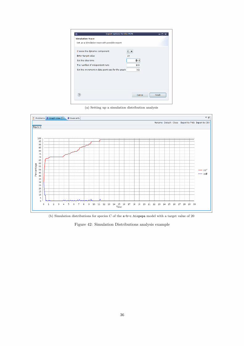
Performing many stochastic simulations provides an opportunity to obtain many more statistics abouta model. One possibility is to obtain the percentage of simulations for which some property is true ator before a given time t. The menu item Simulation Distributions opens a wizard which uses stochasticsimulation to perform this kind of analysis.

The condition which must be met in our case is that a chosen component reaches a prescribedpopulation count. The Bio-PEPA Eclipse Plug-in allows you to set up a number of simulation runsand, based on the simulation data, plots the Probability Distribution Function (pdf) and the CumulativeDistribution Function (cdf) of any species in the model, with respect to the target population value.The most interesting of the two distributions is the cdf, which is plotted as a red line. The cdf showsthe percentage of simulation runs in which the chosen species has reached the target population count,at or before a given time t. In order to take advantage of this feature of the Bio-PEPA Eclipse Plug-inyou should set up the simulation by providing values for the following parameters (see Figure 42a):

• Dynamic component — The species with varying population size than you wish to monitor

• Target value — The condition which your model must meet, i.e. the population size your chosencomponent has to reach

• Stop time — The stop time for the simulation (model dependent)

• Number of independent runs — The number of times the simulation is to be run

• Increment in data point size for the graph — the time-difference between consecutive data pointsin the graph

The pdf and cdf for species C of the a-b-c.biopepa model, with a target value of 20, a stop time of30, 100 independent runs and a 0.1 increment in data point size for the graph, can be seen in Figure 42b.The most interesting of the two distributions is the cdf (red line) which shows, at time t, in how manyof the simulation runs the condition we have set is true, i.e. the population of C has reached the targetvalue, at that time or before. For instance, in 95% of the simulation runs the population of C has reachedthe target value of 20 at or before 10s.

35

(a) Setting up a simulation distribution analysis

(b) Simulation distributions for species C of the a-b-c.biopepa model with a target value of 20

Figure 42: Simulation Distributions analysis example

36

12 Export Wizard

The Bio-PEPA Eclipse Plug-in export wizard translates your Bio-PEPA model to a Systems BiologyMarkup Language (SBML) model (see [6, 15]) for more information on SBML), as shown in Figure 43and produces an .xml export file.

Figure 43: Export Wizard

37

13 Simulation Trace

The Simulation Trace option allows the user to set up the parameters for a simulation run (or a numberof independent simulation runs) and export the simulation trace to three different types of files, namely:

• Traviando export file (.xml file)— export file for Traviando, a trace analyzer and visualizer forsimulation traces of discrete event dynamic systems (see [8, 18, 16, 17, 24, 12, 26, 13, 9] for moreinformation on Traviando)

• BioNessie export file (.bn file)— export file for BioNessie, a free, state-of-the-art platform-independentbiochemical networks simulation and analysis software environment (see [2, 25] for more informationon BioNessie)

• SBRML results export file (.sbrml file)— results export file for Systems Biology Markup Language(SBML) (see [6, 15] for more information on SBML)

In order to set up the simulation the user is allowed to set several parameters (see Figure 44a):

• Number of firings limit — A limit to the number of reactions that can occur (optional)

• Time limit for the trace — The stop time of the simulation (optional)

• Output comments - Enter a comment — If the user checks the output comments checkbox theyare allowed to add a comment to the export file concerning the function of the model

• Show results graph - Set the increment in data point size for the graph — If the user checks theappropriate checkbox the results of the simulation are plotted in a graph. In this case the user canset the time difference between consecutive data points in the graph (default value 1.0)

• Number of independent runs — The number of simulation traces to be produced (default value 1)

The simulation set up for the a-b-c.biopepa model, as shown in Figure 44a, produces three exportfiles, the .bn BioNessie export file, the .sbrml SBML results export file and the .xml Traviando exportfile. The simulation trace data are also plotted in a graph, as shown in Figure 44b.

38

(a) Setting up a simulation for the a-b-c.biopepa model

(b) Graph results of the simulation for the a-b-c.biopepa model

Figure 44: Simulation Trace

39

A The Bio-PEPA plugin syntax

This is a brief overview of the basic elements of the Bio-PEPA Eclipse Plug-in syntax and is by no meanscomprehensive. For more information on the Bio-PEPA Eclipse Plug-in syntax and its differences withBio-PEPA see [14, 11].

A biological system can be encoded as a Bio-PEPA model by way of a 6-tuple [14]:

〈V,N,K, FR, Comp, P 〉

where:

• V is the set of locations

• N is the set of species attributes

• K is the set of parameter definitions

• FR is the set of functional rates

• Comp is the set of species components

• P is the model component

The following sections will explain this definition by describing its constituent elements in moredetail. Sections A.7 - A.10 will offer examples of models defined using the Bio-PEPA language and theBio-PEPA Eclipse Plug-in syntax.

A.1 Locations

Each location must encode an identifier, the parent location, the size of the location (s ∈ R), the typethe location represents and the step-size (H ∈ N?) for the location [14].

The concrete syntax, as accepted by the plug-in is as follows (angular brackets (〈 〉) denote optionalparts in the definition):

location ID 〈in parentID〉 : size = value 〈, step− size = value〉 〈, type = {membrane, compartment}〉;

The keyword location labels the purpose of this definition. The keyword must be proceeded by the IDfor this new location. If the model defines multiple locations, the spatial location can be specified byadding the keyword in and the ID for the parent. The size is the only required property in the locationdefinition (where value ∈ R), while the type is optional as it defaults to compartment. The step-size(value ∈ N∗) is only required if performing analysis of a Bio-PEPA model with levels (for more detailssee [11]). If no locations are defined the default location is used, which is a compartment labelled mainwith size equal to one [14]. As an example, in sections A.8 - A.10, in the Unidireactional and BidirectionalTransportation examples, there are two locations specified:

location main : size = 2, type = membrane;

location child in main : size = 1;

The first location is a membrane of size 2 with ID main and the second is a compartment with IDchild and size equal to 1. In the second definition, the type is not declared as it defaults to compartment.

A.2 Species Attributes

The concrete syntax for the species attributes, as accepted by the plug-in is as follows [14]:

species speciesID : upper = value 〈, lower = value〉;

where speciesID is one of the following [14]:

41

• speciesID Referring to just the species identifier is seen as a global reference. If a species can existin three locations and a reaction is stated in terms of the species, then the reaction is assumed tobe defined as occurring in all three locations independently of each other.

• speciesID@locationID This allows a reference to a specific species in a specific location. If areaction is defined in this manner it will not be enabled in other locations that the species can existin.

• speciesID@locID1, ..., locIDn If a reference to a species in more than one location, but not all,is required then a comma delimited list can be used. This allows fine-grained control over wherethe definition in question is applicable.

The only required attribute in the definition is the upper bound (value ∈ N?), as the default lowerbound is the value zero. If an improved lower bound is known then it can also be specified (value ∈ N?)[14].

Some examples of species attribute definition for a species S follow:

species S : upper = 40, lower = 10;

species S@main : upper = 40, lower = 10;

species S@main,child : upper = 40, lower = 10;

In the first definition species S is defined globally, while in the following definitions it is defined inspecific locations (S@main, S@main,child).

A.3 Parameter Definitions

The concrete syntax for parameter definitions, as accepted by the plug-in, is as follows [14]:

ID = expression;

where

expression = int | float | ID | speciesID | (expr) | expr + expr |expr − expr | expr/expr | expr ∗ expr

An expression is any standard mathematical expression with the definition structured as it is becauseof the recursive nature of the expression (expr is an abbreviation for expression, and not a different set ofallowable expressions). Also, speciesID must refer to a species in a single location if multiple locationsare specified [14]. Some examples of parameter definitions are shown below:

r = 1.0;

r = A - B;

r = A@main + B;

where A, A@main and B are speciesIDs.

A.4 Functional Rates

The concrete syntax for the functional rates, as accepted by the plug-in, is as follows [14]:

kineticLawOf ID : expression′;

or

ID = [ expression′ ];

where expression′ extends the previous expression statement (see section A.3) to also include pre-definedkinetic rates as shown in [14]:

expression′ = expression | fMA(expr) | fMM(expr, expr)

42

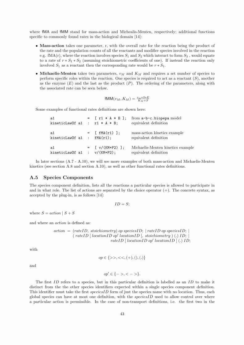
where fMA and fMM stand for mass-action and Michealis-Menten, respectively; additional functionsspecific to commonly found rates in the biological domain [14]:

• Mass-action takes one parameter, r, with the overall rate for the reaction being the product ofthe rate and the population counts of all the reactants and modifier species involved in the reactione.g. fMA(r), where the reaction involves species S1 and S2 which interact to form S3 , would equateto a rate of r ∗ S1 ∗ S2 (assuming stoichiometric coefficients of one). If instead the reaction onlyinvolved S1 as a reactant then the corresponding rate would be r ∗ S1.

• Michaelis-Menten takes two parameters, vM and KM and requires a set number of species toperform specific roles within the reaction. One species is required to act as a reactant (S), anotheras the enzyme (E) and the last as the product (P ). The ordering of the parameters, along withthe associated rate can be seen below.

fMM(vM ,KM ) = vm∗S∗EKM+S

Some examples of functional rates definitions are shown here:

a1 = [ r1 * A * B ]; from a-b-c.biopepa modelkineticLawOf a1 : r1 * A * B; equivalent definition

a1 = [ fMA(r1) ]; mass-action kinetics examplekineticLawOf a1 : fMA(r1); equivalent definition

a1 = [ v/(KM+P2) ]; Michaelis-Menten kinetics examplekineticLawOf a1 : v/(KM+P2); equivalent definition

In later sections (A.7 - A.10), we will see more examples of both mass-action and Michaelis-Mentenkinetics (see section A.8 and section A.10), as well as other functional rates definitions.

A.5 Species Components

The species component definition, lists all the reactions a particular species is allowed to participate inand in what role. The list of actions are separated by the choice operator (+). The concrete syntax, asaccepted by the plug-in, is as follows [14]:

ID = S;

where S = action | S + S

and where an action is defined as:

action = (rateID, stoichiometry) op speciesID; | rateID op speciesID; |( rateID [ locationID op′ locationID ], stoichiometry ) (.) ID; |

rateID [ locationID op′ locationID ] (.) ID;

with

op ∈ {>>,<<, (+), (), (.)}

and

op′ ∈ {− >,< − >}.

The first ID refers to a species, but in this particular definition is labelled as an ID to make itdistinct from the the other species identifiers expected within a single species component definition.This identifier must take the first speciesID form of just the species name with no location. Thus, eachglobal species can have at most one definition, with the speciesID used to allow control over wherea particular action is permissible. In the case of non-transport definitions, i.e. the first two in the

43

action definition, the speciesID can take any of the previously defined forms. Thus a single reactioncan be defined as occurring in the global sense for the species, in a single location, or in a subset of thelocations where the species is present [14]. If a reaction occurs in the global sense for the species, thenthe speciesID identifier may be ommited. For example, in the species components definitions of thea-b-c.biopepa model (see Figure 28a), the speciesID identifier after the operation symbol has beenommited in all of the reactions, as they occur in the global sense :

A = a1 << + a3 >> ;

This is equivalent to:

A = a1 << A + a3 >> A;

The identifiers labelled rateID must refer to a previously defined functional rate. Additionally,stoichiometry is the stoichiometric coefficient for the species in this reaction(stoichiometry ∈ N?). If astatement does not specify a stoichiometric coefficient, the default value of one is used. The definitionfor action shows the syntax for including the stoichiometric coefficient and the abbreviated form forwhen the stoichiometry is one, these being the first two forms shown in the action definition above [14].For example, in the species components definitions of the a-b-c.biopepa model (see Figure 28a), thestoichiometric coefficient has been omitted, since it has the value of 1 in all cases:

A = a1 << + a3 >> ;

This is equivalent to:

A = (a1,1) << + (a3,1) >> ;

And also equivalent to:

A = (a1,1) << A + (a3,1) >> A;

Transportation represents the movement of a single species between two adjacent locations withinthe model, as described in [10]. In the defined syntax above (third and fourth action definitions) itrequires two locationIDs, the first acting as the source and the second as the target and must refer tolocations that this particular species resides in. As the locations are embedded within the transporta-tion action, the identifier is simply the species name. The general modifier operator ((.)) is used fortransportation as, while the levels of the species in the two locations change, the overall amount doesnot. Transportation can either be in a single direction or in both directions (unidirectional or bidi-rectional transportation respectively) [14]. For an example of the unidirectional and the bidirectionaltransportation see section A.9 and section A.10, respectively.

For the Bio-PEPA Eclipse Plug-in user’s convenience, many of the original Bio-PEPA mathematicalsymbols have been replaced with textual representations that are available on every keyboard. Table 1contains the Bio-PEPA symbols and their ASCII representations in the Bio-PEPA Eclipse Plug-in [14]:

Behaviour BioPEPA symbol ASCII representationreactant ↑ <<

product ↓ >>

activator ⊕ (+)

inhibitor (-)

modifier � (.)

unidirectional transportation → ->

bidirectional transportation ↔ <->

Table 1: Bio-PEPA mathematical symbols and Bio-PEPA Eclipse Plug-in symbol representation

44

A.6 Model Component

The model component is always the final definition in a Bio-PEPA model. A distinction has to be madebetween the model component definition and labelled compositional definitions. To offer compositionalitythe tool needs to accept fragments of the model component and allow the assigning of a label for reference.Essentially the definitions are nearly identical, with the difference being the assignment of an identifierand the use of the termination symbol. The concrete syntax for labelled compositional definitions, asaccepted by the plug-in is as follows [14]:

ID ::= P ;

where

P = ID | (P ) | P < L > P | speciesID[value] )

where

Behaviour BioPEPA symbol ASCII representationcooperation BC

L<L>

Table 2: Bio-PEPA mathematical symbols and Bio-PEPA Eclipse Plug-in cooperation symbol

Unlike the model component, labelled compositional definitions require an identifier for reference inthe model component. The assignment symbol differs here from other definitions, taking the form of ::=which uniquely identifies the definition type. The compositional fragment comes next, taking one of theforms described above. It can consist of an identifier for another labelled compositional definition, singlespecies or the synchronisation of several species or identifiers [14].

The term P < L > Q denotes cooperation between P andQ over the cooperation set L, that determinesthose activities on which the cooperands are forced to synchronise. For action types not in L, thecomponents proceed independently and concurrently with their enabled activities [11]. The cooperationset, indicated by the symbol L, can either be the wildcard token (?) or a comma delimited list of actions[14].

The model component follows the same syntax as the labelled compositional definition without theassignment or the terminator symbol. In the syntax above, the model component is simply P [14].

An example of a model component definition was the one in the a-b-c.biopepa model (see Fig-ure 28a):

A[initial A] <*> B[initial B] <*> C[initial C]

where <*> denotes cooperation between the species over all reactions, since the cooperation set is the wild-card token (?), and initial A, initial B and initial C are variables that hold the species initial populationcounts.

We will see several more examples of model component definitions in sections A.7 - A.10.

45

A.7 Syntax Example: The Enzyme-Substrate model - Reactant and Product

In this example (see Table 3), an enzyme E combines with a substrate S to form a compound E:S. Thiscompound might degrade releasing the enzyme and the substrate or it might convert the substrate intoproduct P, releasing the enzyme (In the Bio-PEPA Eclipse Plug-in editor the two parallel diagonal lines(//) denote comments). The Outline View of the model is shown in Figure 45. According to the speciescomponents definition:

• E — is a reactant (↓, <<) in reaction r1 and a product (↑, >>) in reactions rm1 and r2

• S — is a reactant (↓, <<) in reaction r1 and a product (↑, >>) in reaction rm1

• E : S — is a product (↓, <<) in reaction r1 and a reactant (↑, >>) in reactions rm1 and r2

• P — is a product in reaction r2

The Bio-PEPA syntax //The Bio-PEPA plugin syntax

Parameter Definitions: //Parameter Definitions

k1 = 0.01; k1 = 1.0;

km1 = 0.01; km1 = 0.1;

k2 = 0.01; k2 = 0.01;

Functional Rates //Functional Rates

r1 = k1 ∗ E ∗ S; r1 = [ k1 * E * S ];

rm1 = km1 ∗ E : S; rm1 = [ km1 * E:S ];

r2 = k2 ∗ E : S; r2 = [ k2 * E:S ];

Species Components //Species Components

Edef= (r1, 1) ↓ E + (rm1, 1) ↑ E + (r2, 1) ↑ E E = r1 << + rm1 >> + r2 >> ;

Sdef= (r1, 1) ↓ S + (rm1, 1) ↑ S S = r1 << + rm1 >> ;

E : Sdef= (r1, 1) ↑ E : S + (rm1, 1) ↓ E : S + (r2, 1) ↓ E : S E:S = r1 >> + rm1 << + r2 << ;

Pdef= (r2, 1) ↑ P P = r2 >> ;

Model Component //Model Component

E[40] BC∗ S[30] BC∗ E : S[0] BC∗ P [0] E[40] <*> S[30] <*> E:S[0] <*> P[0]

Table 3: Bio-PEPA mathematical syntax and Bio-PEPA Eclipse Plug-in syntax for the Enzyme-Substratemodel

46

Figure 45: The Outline View of the Enzyme-Substrate model

A.8 Syntax Example: Activator and Inhibitor

As an example, we will use a model of a general genetic network with a negative feedback throughdimmers (see Figure 46).

Figure 46: Genetic Network model

The model, which is shown in Table 4, is composed of three biological entities that interact with eachother through five reactions (of which one is reversible). The biological entities are the mRNA molecule(M), the protein in monomer form (P ) and the protein in dimeric form (P2). The first reaction (1) isthe transcription of the mRNA (M) from the genes/DNA (not considered explicitly). The protein P inthe dimer form (P2), which is the final result of the network, has an inhibitory effect (, (-)) on thisprocess. The second reaction (2) is the translation of the protein P from M , in which M acts as an

47

activator (⊕, (+)). The other two reactions represent the degradation of M (3) and the degradation of P(4). Finally there is the dimerization of P and its inverse process (5, 5i). All the reactions are describedby mass-action kinetics with the exception of the first reaction, which has a Michaelis-Menten kinetics[11] (see section A.4 for more information on mass-action and Michaelis-Menten kinetics) .

The Outline View of the model can be seen in Figure 47.

The Bio-PEPA syntax //The Bio-PEPA plugin syntaxLocations: //Locations

vcell : 1(nM)−1 location v cell: size = 1;

Parameter Definitions //Parameter DefinitionsKM = 356nM ; KM = 356;

v = 2.19s−1; v = 2.19;

k2 = 0.043s−1; k2 = 0.043;

k3 = 0.039s−1; k3 = 0.039;

k4 = 0.0007s−1; k4 = 0.0007;

k5 = 0.025s−1; k5 = 0.025;

k5i = 0.5s−1; k5i = 0.5;

Species AttributesM : H = 1, N = 1, V = vcell, unit = nM ;P : H = 30, N = 2, V = vcell, unit = nM ;P2 : H = 30, N = 6, V = vcell, unit = nM ;

Functional Rates //Functional Ratesfα1 = v

KM+P2 ; a1 = [v/(KM+P2)];

fα2= fMA(k2); a2 = [fMA(k2)];

fα3= fMA(k3); a3 = [fMA(k3)];

fα4= fMA(k4); a4 = [fMA(k4)];

fα5 = fMA(k5); a5 = [fMA(k5)];fα5i

= fMA(k5i); a5i = [fMA(k5i)];

Species Components //Species Components

Mdef= (α1, 1) ↑M + (α2, 1)⊕M + (α3, 1) ↓M M = a1 >> + a2 (+) + a3 << ;

Pdef= (α2, 1) ↑ P + (α4, 1) ↓ P + (α5, 2) ↓ P + (α5i

, 2) ↑ P P = a2 >> + a4 << + (a5,2) << + (a5i,2) >>;

P2def= (α1, 1) P2 + (α5, 1) ↑ P2 + (α5i

, 1) ↓ P2 P2 = a1 (-) + a5 >> + a5i <<;

Model Component //Model Component

M [0] BCα2P [0] BC

α5,α5iP2[0] M[0] <a2> P[0] <a5, a5i> P2[0]

Table 4: Bio-PEPA mathematical syntax and Bio-PEPA Eclipse Plug-in syntax for the Genetic Networkmodel

Figure 47: The Outline View of the Genetic Network model

48

A.9 Syntax Example: Unidirectional Transportation, Modifier

Figure 48: Locations of the model

The model shown in Table 5 has two locations, the parent location which is called main and is amembrane, and the child location which is a compartment enclosed by the membrane (see Figure 48).In the definition of location child, the type is not declared as it defaults to compartment. The modelcontains two species A and B. Species A is originally located in membrane main (A@main). SpeciesA is involved in the tr reaction, which is a unidirectional transportation reaction (→, ->) representingthe movement of species A from membrane main to compartment child. It is governed by a kineticparameter r1, which controls the rate of the transportation. Parameter r1 has been given the constantvalue of 0.01. The rate of tr also depends on the quantity of A available in main (A@main). Moreover,species A@child and B are involved in the re reaction, which takes plase in compartment child. The rateof re is governed by kinetic parameter r2 which has been given the constant value of 0.01. The rate oftr also depends on the quantity of A available in compartment child (A@child). The quantity of speciesB that is produced is located in child, where re takes place.

As we can see, in the species components definition the general modifier operator (�, (.)) is usedfor transportation as, while the levels of species A in the two locations change, the overall amount doesnot.

The Outline View of the model can be seen in Figure 49.

The Bio-PEPA syntax //The Bio-PEPA plugin syntax

Locations: //Locations

L = [child : 1(nM)−1, C; location child in main : size = 1;

main : 2(nM)−1,M ; ] location main : size = 2, type = membrane;

Parameter Definitions //Parameter Definitions

r1 = 0.01; r1 = 0.01;

r2 = 0.01; r2 = 0.01;

//Variables for the species initial populations

Am = 100;

Ac = 0;

B = 0;

Functional Rates //Functional Rates

ftr = [r1 ∗A@main]; tr = [r1 * A@main];

fre = [r2 ∗A@child]; re = [ r2 * A@child];

Species Components //Species Components

Adef= (tr[main→ child], 1)�A + (re, 1) ↓ A A = tr[main->child] (.) A + re << A@child;

Bdef= (re, 1) ↑ B B = re >>;

Model Component //Model Component

A@main[100] BCtr

A@child[0] BCre

B@child[0] A@main[Am]<tr>A@child[Ac]<re>B@child[B]

Table 5: Bio-PEPA mathematical syntax and Bio-PEPA Eclipse Plug-in syntax for the UnidirectionalTransportation model

49

Figure 49: The Outline View of the Unidirectional Transportation model

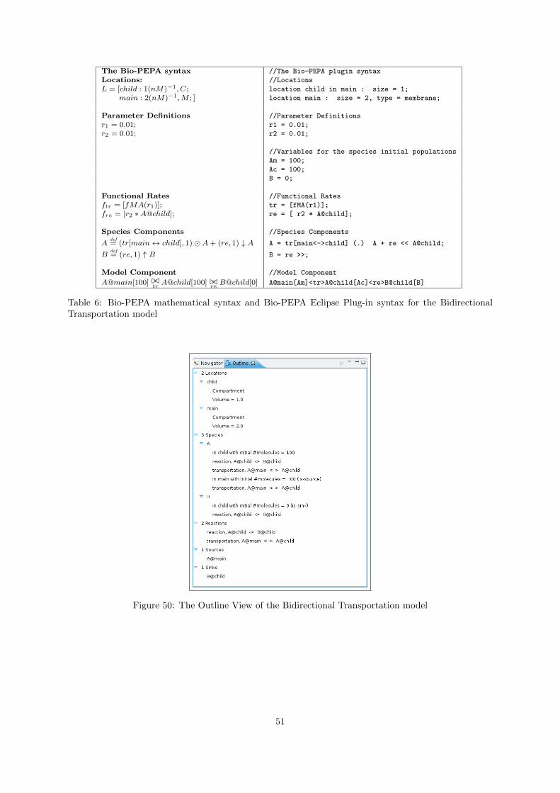
A.10 Syntax Example: Bidirectional Transportation, Modifier

The model shown in Table 6 has two locations, the parent location which is called main and is amembrane, and the child location which is a compartment enclosed by the membrane (see Figure 48).In the definition of location child, the type is not declared as it defaults to compartment. The modelcontains two species A and B. Species A is originally located both in membrane main (A@main) andin compartment child (A@child). Species A is involved in the tr reaction, which is a bidirectionaltransportation (↔, <->) reaction representing the movement of species A from membrane main tocompartment child and vice versa. The tr reaction is described by mass-action kinetics (fMA(r1)),where r1 is a kinetic parameter that has been given the constant value of 0.01 (see section A.4 for moreinformation on mass-action kinetics). Moreover, species A@child and B are involved in the re reaction,which takes plase in compartment child. The rate of re is governed by kinetic parameter r2 which hasbeen given the constant value of 0.01. The rate of tr also depends on the quantity of A available incompartment child (A@child). The quantity of species B that is produced is located in child, where retakes place.

In the species components definition, the general modifier operator (�, (.)) is used for transportationas, while the levels of species A in the two locations change, the overall amount does not.

The Outline View of the model can be seen in Figure 50.

50

The Bio-PEPA syntax //The Bio-PEPA plugin syntax

Locations: //Locations

L = [child : 1(nM)−1, C; location child in main : size = 1;

main : 2(nM)−1,M ; ] location main : size = 2, type = membrane;

Parameter Definitions //Parameter Definitions

r1 = 0.01; r1 = 0.01;

r2 = 0.01; r2 = 0.01;

//Variables for the species initial populations

Am = 100;

Ac = 100;

B = 0;

Functional Rates //Functional Rates

ftr = [fMA(r1)]; tr = [fMA(r1)];

fre = [r2 ∗A@child]; re = [ r2 * A@child];

Species Components //Species Components

Adef= (tr[main↔ child], 1)�A + (re, 1) ↓ A A = tr[main<->child] (.) A + re << A@child;

Bdef= (re, 1) ↑ B B = re >>;

Model Component //Model Component

A@main[100] BCtr

A@child[100] BCre

B@child[0] A@main[Am]<tr>A@child[Ac]<re>B@child[B]

Table 6: Bio-PEPA mathematical syntax and Bio-PEPA Eclipse Plug-in syntax for the BidirectionalTransportation model

Figure 50: The Outline View of the Bidirectional Transportation model

51

B Managing Eclipse

B.1 Checking the Eclipse platform version

To check which version of the Eclipse platform you have installed choose Help → About Eclipse (seeFigure 51).

Figure 51: Checking the version of the Eclipse platform

In the dialogue box that appears you can see the version of the Eclipse platform that you haveinstalled (see Figure 52).

Figure 52: Information on the version of the Eclipse platform

For more detailed information on your Eclipse installation, you can click on the Installation

Details button. In Figure 53 you can see the window which contains the details on the Eclipse in-stallation.

52

Figure 53: More information on the Eclipse platform installation

B.2 Checking for Updates

To check for updates of the Bio-PEPA software and the Eclipse platform choose Help → Check forUpdates (see Figure 54).

Figure 54: Checking for updates

Eclipse will contact its update sites, including the Bio-PEPA update site and fetch the availableupdates (see Figure 55). If you do not want to wait for Eclipse to finish this job, you may choose to runit in the background by clicking on the Run in Background button. You may also choose to always runthis job in the background, by checking the box next to the Always run in background option.

Figure 55: Contacting software sites for updates

Eclipse will then display the available updates. You are required to choose the updates you wish toinstall by checking the corresponding checkbox (see Figure 56). Then, click Next.

53

Figure 56: Displaying the available updates

Eclipse will display the updates you have chosen to install and give you the opportunity to reviewthem and confirm your choice (see Figure 57). After you have done so, click Next.

Figure 57: Review and confirm updates

Then, accept the terms of the licence agreement before clicking on Finish (see Figure 58).

54

Figure 58: Review and accept licences

Eclipse will install the updates (see Figure 59). Again, you may choose to run this job in thebackground by clicking on the Run in Background button. You may also choose to always run it in thebackground, by checking the box next to the Always run in background option.

Figure 59: Updating software

After the installation is complete, a dialogue box will appear informing you that, for the updates totake place, you should restart Eclipse. You can also try to apply the changes without restarting, butthis might cause errors. We recommend restarting Eclipse to apply the updates.

The dialogue box gives you three options. You can leave the changes for later, in which case they willbe applied the next time you start Eclipse, by clicking on the Not Now button. You can try to applythe changes without restarting, by clicking on the Apply Changes Now button. Finally, you can restartEclipse, so that the changes are applied properly, by clicking on the Restart Now button. The last choiceis the recommended one (see Figure 60).

Figure 60: Applying the changes

55

References

[1] The bio-pepa modelling language. http://www.biopepa.org/.

[2] The bionessie biochemical networks simulation and analysis software environment. http://disc.

brunel.ac.uk/bionessie/.

[3] The eclipse open development platform. http://www.eclipse.org/.

[4] The prism probabilistic model checker. http://www.prismmodelchecker.org/.

[5] The simulation experiment description markup language (sed-ml). http://sedml.org/.

[6] The systems biology markup language (sbml). http://sbml.org.

[7] The systems biology software infrastructure (sbsi). http://www.sbsi.ed.ac.uk/index.html.

[8] The traviando simulation trace analyzer and visualizer. http://www.cs.wm.edu/~kemper/

Traviando.html.

[9] Proceedings of the 2010 Winter Simulation Conference, WSC 2010, Baltimore, Maryland, USA, 5-8December 2010. WSC, 2010.

[10] F. Ciocchetta and M. L. Guerriero. Modelling biological compartments in bio-pepa. Electron. NotesTheor. Comput. Sci., 227:77–95, Jan. 2009.

[11] F. Ciocchetta and J. Hillston. Bio-pepa: A framework for the modelling and analysis of biologicalsystems. Theor. Comput. Sci., 410(33-34):3065–3084, Aug. 2009.

[12] A. Clark, S. Gilmore, M. L. Guerriero, and P. Kemper. On verifying bio-pepa models. In Quaglia[26], pages 23–32.

[13] A. Clark, J. Hillston, S. Gilmore, and P. Kemper. Verification and testing of biological models. InWinter Simulation Conference [9], pages 620–630.

[14] A. Duguid. An overview of the bio-pepa eclipse plug-in. In PASTA 2009, 8th Workshop on ProcessAlgebra and Stochastically Timed Activities, pages 121–131, August 2009.

[15] M. Hucka, A. Finney, H. M. Sauro, H. Bolouri, J. C. Doyle, H. Kitano, , the rest of the SBML Forum:,A. P. Arkin, B. J. Bornstein, D. Bray, A. Cornish-Bowden, A. A. Cuellar, S. Dronov, E. D. Gilles,M. Ginkel, V. Gor, I. I. Goryanin, W. J. Hedley, T. C. Hodgman, J.-H. Hofmeyr, P. J. Hunter, N. S.Juty, J. L. Kasberger, A. Kremling, U. Kummer, N. Le Novre, L. M. Loew, D. Lucio, P. Mendes,E. Minch, E. D. Mjolsness, Y. Nakayama, M. R. Nelson, P. F. Nielsen, T. Sakurada, J. C. Schaff,B. E. Shapiro, T. S. Shimizu, H. D. Spence, J. Stelling, K. Takahashi, M. Tomita, J. Wagner, andJ. Wang. The systems biology markup language (sbml): a medium for representation and exchangeof biochemical network models. Bioinformatics, 19(4):524–531, 2003.

[16] P. Kemper. Recent extensions to traviando. In Quantitative Evaluation of Systems, 2009. QEST’09. Sixth International Conference on the, pages 283 –284, sept. 2009.

[17] P. Kemper. Report generation for simulation traces with traviando. In Dependable Systems Net-works, 2009. DSN ’09. IEEE/IFIP International Conference on, pages 347 –352, 29 2009-july 22009.

[18] P. Kemper and G. Tepper. Traviando - debugging simulation traces with message sequence charts.In Quantitative Evaluation of Systems, 2006. QEST 2006. Third International Conference on, pages135 –136, sept. 2006.

[19] D. Kohn and N. Le Novere. SED-ML An XML Format for the Implementation of the MIASEGuidelines, volume 5307, pages 176–190. Springer Berlin / Heidelberg, 2008.

56

[20] M. Kwiatkowska, G. Norman, and D. Parker. PRISM: Probabilistic symbolic model checker. InP. Kemper, editor, Proc. Tools Session of Aachen 2001 International Multiconference on Mea-surement, Modelling and Evaluation of Computer-Communication Systems, pages 7–12, September2001.

[21] M. Kwiatkowska, G. Norman, and D. Parker. PRISM 2.0: A tool for probabilistic model checking.In Proc. 1st International Conference on Quantitative Evaluation of Systems (QEST’04), pages322–323. IEEE Computer Society Press, 2004.

[22] M. Kwiatkowska, G. Norman, and D. Parker. Prism: Probabilistic model checking for performanceand reliability analysis. ACM SIGMETRICS Performance Evaluation Review, 36(4):40–45, 2009.

[23] M. Kwiatkowska, G. Norman, and D. Parker. PRISM 4.0: Verification of probabilistic real-timesystems. In G. Gopalakrishnan and S. Qadeer, editors, Proc. 23rd International Conference onComputer Aided Verification (CAV’11), volume 6806 of LNCS, pages 585–591. Springer, 2011.

[24] R. Lamprecht and P. Kemper. Mobius trace analysis with traviando. In Quantitative Evaluation ofSystems, 2008. QEST ’08. Fifth International Conference on, pages 41 –42, sept. 2008.

[25] X. Liu, J. Jiang, O. Ajayi, X. Gu, D. Gilbert, and R. Sinnott. Bionessie(g) - a grid enabled biochem-ical networks simulation environment. Studies In Health Technology And Informatics, 138:147–157,2008.

[26] P. Quaglia, editor. Computational Methods in Systems Biology, 8th International Conference, CMSB2010, Trento, Italy, September 29 - October 1, 2010. Proceedings. ACM, 2010.

[27] D. Waltemath, R. Adams, F. Bergmann, M. Hucka, F. Kolpakov, A. Miller, I. Moraru, D. Nickerson,S. Sahle, J. Snoep, and N. Le Novere. Reproducible computational biology experiments with sed-ml- the simulation experiment description markup language. BMC Systems Biology, 5(1):198, 2011.

57