0

PEPA or Bio-PEPA: A Comparison

Erin Gemma Scott

Registration No: 1611732

April 2011

Dissertation submitted in partial fulfilment for the degree of Computing Science

Department of Computing Science and Mathematics University of Stirling

1

Abstract Problem Process algebra offers a unique opportunity in the biological context for modelling information of biological processes. PEPA (Performance Evaluation Process Algebra) and Bio-PEPA (Biochemical Performance Process Algebra) are expressive formal languages for modelling distributed systems. Bio-PEPA is a modification of PEPA, with extended special features for biological systems. Starting with the hypothesis that indicates Bio-PEPA should be better than PEPA for biological systems, the principal aim of this project was to test this hypothesis through a number of case studies. The final outcome of the project is a recommendation based on system features and analysis requirements to allow a user to choose the most appropriate language for their specific biological system. Objectives The project assists with decisions on which language would be appropriate as a result of the comparison analysis of specific case studies. The case studies were of high and low level biological systems from individual cells to crowd dynamics of humans. Each of the case studies incorporated specific biological features; space, timed events, birth and death, inhibition and promotion and phenotypic switching. A number of the case studies had experimental data therefore allowing comparison with both process algebra model results. The three case studies investigated and implemented highlighted specific language features and analysis techniques in both languages. The project will further aid in the preliminary study and application of the languages. The project allows the checking of claims made for both languages, giving a better understanding of using PEPA and Bio-PEPA. The recommendations show the benefits of both languages and their analysis techniques in application to biological systems. Methodology An iterative method was undertaken. The steps included initially reviewing different case studies of biological networks in either language. Subsequently appropriate case studies were selected and implemented in the alternate language. The implementation of each case study in the alternate language was achieved through a number of simple models building to more complex models. Thereafter, analysis of the strengths and weaknesses of both models in terms of language features and analysis techniques was undertaken. Subsequently adding recommendations to and testing the hypothesis. This built a full set of recommendations with regard to the original hypothesis. Achievements Knowledge of PEPA and Bio-PEPA languages and analysis techniques was gained. The investigation of three biological case studies was carried out. This included an evaluation of the literature of the particular case studies, the replication of the original models, the implementation and analysis of the alternate language models and the comparison analysis with the original models and original data where available. Recommendations were created based on system features and analysis requirements of both languages to allow a user to choose the most appropriate language for their specific biological system.

2

Attestation I understand the nature of plagiarism, and am aware of the University’s policy on this. I certify that this dissertation reports original work by me during my University project except for the following:

• The example Bio-PEPA model in section 2.2.2 was replicated from the paper, Bio-PEPA: A Framework for the Modelling and Analysis of Biochemical Networks [5].

• The replication of the model in section 3.2 was from the paper, Modelling Crowd Dynamics in Bio-PEPA- Extended Abstract [7].

• The replication of the model in section 2.1.3 was from the paper, Modelling Immunological Systems using PEPA: a preliminary report [4]. The model was developed by me during a vacation placement at the University of Stirling.

• The replication of the model in section 5.2 was from the thesis, Process algebra and epidemiology: evaluating the ability of PEPA to describe biological systems [11].

Signature Date 21 April 2011

3

Acknowledgements I would particularly wish to acknowledge and thank my supervisor Dr Carron Shankland for her constant support, encouragement and guidance throughout this project. I would also wish to thank Soufiene Benkirane for his invaluable input for modelling in PEPA and I am grateful to him for providing his measles epidemiology PEPA model. I am also grateful to Dr Andrea Graham (Department of Ecology and Evolutionary Biology, Princeton University) for her knowledge and assistance in immunological systems and for providing the data for the immunological systems model. I express thanks to Maria Luisa Guerriero (Centre for Systems Biology at the University of Edinburgh) for her assistance with Bio-PEPA and especially with events in Bio-PEPA. On a personal note, I wish to express my appreciation to my Mum and Dad for their continuous support and encouragement with my studies, without which I would have been unable to have accomplished half as much as I have.

4

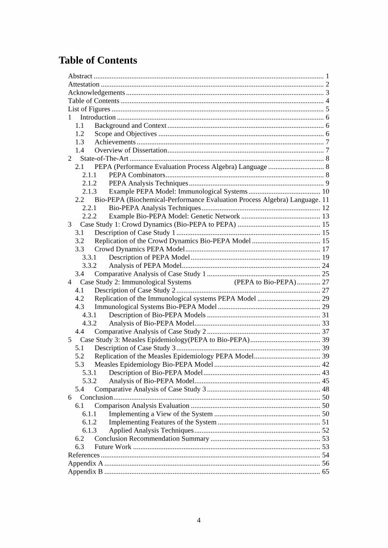
Table of Contents Abstract ................................................................................................................................ 1 Attestation ............................................................................................................................ 2 Acknowledgements .............................................................................................................. 3 Table of Contents ................................................................................................................. 4 List of Figures ...................................................................................................................... 5 1 Introduction ................................................................................................................... 6

1.1 Background and Context ....................................................................................... 6 1.2 Scope and Objectives ............................................................................................ 6 1.3 Achievements ........................................................................................................ 7 1.4 Overview of Dissertation ....................................................................................... 7

2 State-of-The-Art ............................................................................................................ 8 2.1 PEPA (Performance Evaluation Process Algebra) Language ............................... 8

2.1.1 PEPA Combinators ........................................................................................ 8 2.1.2 PEPA Analysis Techniques ........................................................................... 9 2.1.3 Example PEPA Model: Immunological Systems ........................................ 10

2.2 Bio-PEPA (Biochemical-Performance Evaluation Process Algebra) Language . 11 2.2.1 Bio-PEPA Analysis Techniques .................................................................. 12 2.2.2 Example Bio-PEPA Model: Genetic Network ............................................ 13

3 Case Study 1: Crowd Dynamics (Bio-PEPA to PEPA) .............................................. 15 3.1 Description of Case Study 1 ................................................................................ 15 3.2 Replication of the Crowd Dynamics Bio-PEPA Model ...................................... 15 3.3 Crowd Dynamics PEPA Model ........................................................................... 17

3.3.1 Description of PEPA Model ........................................................................ 19 3.3.2 Analysis of PEPA Model ............................................................................. 24

3.4 Comparative Analysis of Case Study 1 ............................................................... 25 4 Case Study 2: Immunological Systems (PEPA to Bio-PEPA) ............. 27

4.1 Description of Case Study 2 ................................................................................ 27 4.2 Replication of the Immunological systems PEPA Model ................................... 29 4.3 Immunological Systems Bio-PEPA Model ......................................................... 29

4.3.1 Description of Bio-PEPA Models ............................................................... 31 4.3.2 Analysis of Bio-PEPA Model ...................................................................... 33

4.4 Comparative Analysis of Case Study 2 ............................................................... 37 5 Case Study 3: Measles Epidemiology(PEPA to Bio-PEPA) ....................................... 39

5.1 Description of Case Study 3 ................................................................................ 39 5.2 Replication of the Measles Epidemiology PEPA Model ..................................... 39 5.3 Measles Epidemiology Bio-PEPA Model ........................................................... 42

5.3.1 Description of Bio-PEPA Model ................................................................. 43 5.3.2 Analysis of Bio-PEPA Model ...................................................................... 45

5.4 Comparative Analysis of Case Study 3 ............................................................... 48 6 Conclusion ................................................................................................................... 50

6.1 Comparison Analysis Evaluation ........................................................................ 50 6.1.1 Implementing a View of the System ........................................................... 50 6.1.2 Implementing Features of the System ......................................................... 51 6.1.3 Applied Analysis Techniques ...................................................................... 52

6.2 Conclusion Recommendation Summary ............................................................. 53 6.3 Future Work ........................................................................................................ 53

References .......................................................................................................................... 54 Appendix A ........................................................................................................................ 56 Appendix B ........................................................................................................................ 65

5

List of Figures Figure 1. Immunological PEPA Model .............................................................................. 10Figure 2. Genetic Network Bio-PEPA Model .................................................................... 13Figure 3. Genetic Network Model ...................................................................................... 13Figure 4. Simulation graphs from model showing population of component P ................. 14Figure 5. Crowd Dynamics Bio-PEPA Model .................................................................... 15Figure 6. City plan with four squares .................................................................................. 16Figure 7. ODE simulation graphs (a) c = 0.005 (b) c = 0.1 ................................................ 16Figure 8. Individual Agent State Diagram .......................................................................... 17Figure 9. Crowd Dynamics PEPA Model (Partial Code) .................................................. 18Figure 10. Square Centric View code ............................................................................... 19Figure 11. First Development Independent Choice Code ................................................. 21Figure 12. Stochastic simulation graphs- replications = 100 (a) c = 0.005 (b) c = 0.1 ..... 21Figure 13. Second Development Independent Choice Partial Code ................................. 22Figure 14. Stochastic simulation graphs- replications = 100 (a) c = 0.005 (b) c = 0.1 ..... 23Figure 15. Stochastic simulation graphs – replications = 100 (a) c = 0.01 (b) c = 0.25 ... 25Figure 16. Recruitment of Naïve Th cells [15] ................................................................. 27Figure 17. Experimental Results Th1 Population (left) , Th2 Population (right)[18] ....... 28Figure 18. Experimental Time Line and Groups [18] ....................................................... 29Figure 19. Switching Model ............................................................................................. 30Figure 20. Heaviside Step Function Code ........................................................................ 31Figure 21. Example of Malaria Injection Timed Event .................................................... 31Figure 22. MalariaI Value (a) HelminthI Value (b) Simulation Graphs ........................... 32Figure 23. Experiment (a) Rates for Environment Model ................................................ 34Figure 24. Experiment (a) Stochastic Graph for Environment Model .............................. 34Figure 25. Experiment (b) Rates for Environment Model ................................................ 34Figure 26. Experiment (b) Stochastic Graph for Environment Model .............................. 35Figure 27. Experiment (a) Rates for Switching Model ..................................................... 35Figure 28. Experiment (a) Stochastic Graph for Switching Model .................................. 36Figure 29. Experiment (b) Rates for Switching Model ..................................................... 36Figure 30. Experiment (b) Stochastic Graph for Switching Model .................................. 37Figure 31. Table of parameters used in the PEPA model ................................................. 39Figure 32. Measles Epidemiology PEPA Model (Partial Code) ....................................... 40Figure 33. Comparison Graphs of Reconstructed Data and PEPA Model ....................... 41Figure 34. Measles Epidemiology Bio-PEPA Model ....................................................... 42Figure 35. Heaviside Step Function Code ........................................................................ 43Figure 36. Contact Rate Kinetic Law ............................................................................... 43Figure 37. Season_time Value Simulation Graphs ........................................................... 44Figure 38. Simulation Graph of Immigration ................................................................... 45Figure 39. ODE and Stochastic Simulation Graphs .......................................................... 46Figure 40. Comparison Graphs of Bio-PEPA Model (a) and Corrected Data (b) ............ 47

6

1 Introduction

1.1 Background and Context PEPA (Performance Evaluation Process Algebra) and Bio-PEPA (Biochemical Performance Process Algebra) are expressive formal languages for modelling distributed systems. Bio-PEPA is an extension of PEPA, with extended special features for biological systems. PEPA and Bio-PEPA allow the analysis of a system which can determine whether a candidate design meets both the behavioural and the temporal requirements demanded of it. Process algebra offers a unique opportunity in systems biology. Biological systems come in many varieties, for example, individual cells to whole ecosystems. Systems biology is an examination of the structure and dynamics of cellular, organism and ecosystem function, rather than the characteristics of isolated parts of a cell, organism or ecosystem. Many properties of life arise at the systems level only, as the behaviour of the system as a whole cannot be explained by its constituents alone. Process algebra gives a high-level description of interactions, communications, and synchronizations between a collection of independent agents or processes. Its application provides many analysis techniques for the networks behaviour and properties. Starting with the hypothesis that indicates Bio-PEPA should be better than PEPA for biological systems, the principal aim was to test this hypothesis through a number of case studies. The final outcome of the project is a recommendation based on system features and analysis requirements to allow a user to choose the most appropriate language for their specific biological system.

1.2 Scope and Objectives Different case studies of biological networks were reviewed in both PEPA and Bio-PEPA. Three appropriate case studies were selected and implemented and analysed in the alternate language. The reasons for choosing the three case studies were the language features and analysis techniques that they highlight when implementing the networks. The crowd dynamic case study discussed in section 3 was chosen as it had spatial elements and this emphasizes how the two languages handle the implementation of locations in a model. The immunological case study referred in section 4 was chosen as it dealt with experimental data, also how biological inhibition and events are implemented in both languages. The measles epidemiology case study referred in section 5 was chosen as it also had spatial elements, experimental data and the introduction of events to the model. This further developed the understanding and recommendations for the comparison. The case studies were of high and low level biological systems from individual cells to crowd dynamics of humans. Each of the case studies incorporated specific biological features; space, timed events, birth and death, inhibition and promotion and phenotypic switching. Thereafter the criteria for measuring both languages were the examination of the strengths and weaknesses of both models in terms of language features and analysis techniques and subsequently adding recommendations to and testing the hypothesis. The project assists with decisions on which language would be appropriate as a result of the comparison analysis. The project will further aid in the preliminary study and application of the languages by adding to the case study literature. The project also allows the checking of claims made for both languages, giving a better understanding of using PEPA and Bio-PEPA. The recommendations show the benefits of both languages and their analysis techniques in application to biological systems.

7

1.3 Achievements All goals were achieved. In particular knowledge of PEPA and Bio-PEPA languages and analysis techniques was gained. The investigation of three biological case studies was carried out. This included an evaluation of the literature of the particular case studies, the replication of the original models, the implementation and analysis of the alternate language models and the comparison analysis with the original models. The summary of recommendations based on system features and analysis requirements of both languages was implemented to allow a user to choose the most appropriate language for their specific biological system.

1.4 Overview of Dissertation The paper is structured as follows. In the next section ‘State-of-the-art’ a description of the PEPA and Bio-PEPA languages is reported. Section 3 describes the investigation and implementation of case study one in crowd dynamics. After that, in section 4 describes the investigation and implementation of case study two immunological systems. The investigation and implementation of case study three in measles epidemiology is presented in section 5. Section 6 reports the conclusion which includes the evaluation and the summary of recommendations and future investigations.

8

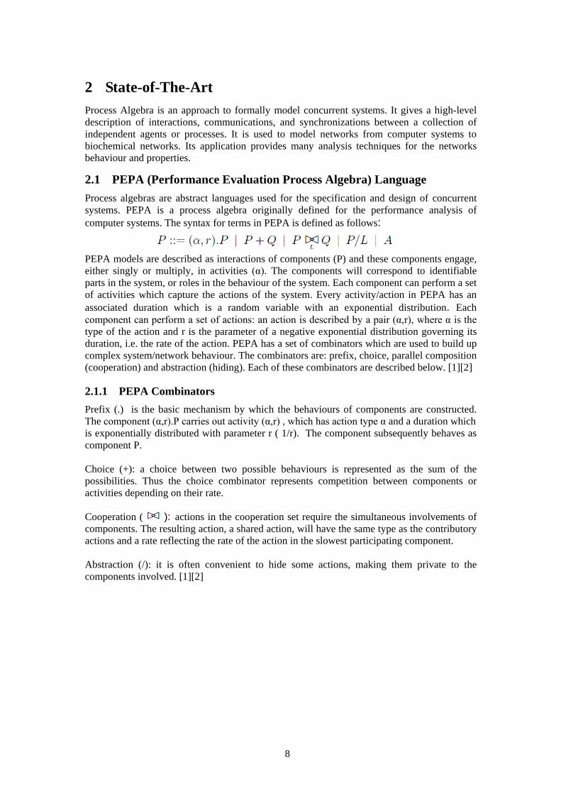
2 State-of-The-Art Process Algebra is an approach to formally model concurrent systems. It gives a high-level description of interactions, communications, and synchronizations between a collection of independent agents or processes. It is used to model networks from computer systems to biochemical networks. Its application provides many analysis techniques for the networks behaviour and properties.

2.1 PEPA (Performance Evaluation Process Algebra) Language Process algebras are abstract languages used for the specification and design of concurrent systems. PEPA is a process algebra originally defined for the performance analysis of computer systems. The syntax for terms in PEPA is defined as follows: PEPA models are described as interactions of components (P) and these components engage, either singly or multiply, in activities (α). The components will correspond to identifiable parts in the system, or roles in the behaviour of the system. Each component can perform a set of activities which capture the actions of the system. Every activity/action in PEPA has an associated duration which is a random variable with an exponential distribution. Each component can perform a set of actions: an action is described by a pair (α,r), where α is the type of the action and r is the parameter of a negative exponential distribution governing its duration, i.e. the rate of the action. PEPA has a set of combinators which are used to build up complex system/network behaviour. The combinators are: prefix, choice, parallel composition (cooperation) and abstraction (hiding). Each of these combinators are described below. [1][2]

2.1.1 PEPA Combinators Prefix (.) is the basic mechanism by which the behaviours of components are constructed. The component (α,r).P carries out activity (α,r) , which has action type α and a duration which is exponentially distributed with parameter r ( 1/r). The component subsequently behaves as component P. Choice (+): a choice between two possible behaviours is represented as the sum of the possibilities. Thus the choice combinator represents competition between components or activities depending on their rate. Cooperation ( ): actions in the cooperation set require the simultaneous involvements of components. The resulting action, a shared action, will have the same type as the contributory actions and a rate reflecting the rate of the action in the slowest participating component. Abstraction (/): it is often convenient to hide some actions, making them private to the components involved. [1][2]

9

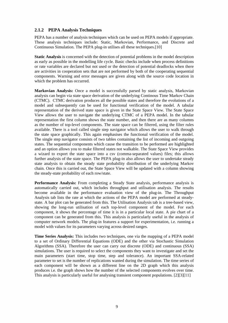
2.1.2 PEPA Analysis Techniques PEPA has a number of analysis techniques which can be used on PEPA models if appropriate. These analysis techniques include: Static, Markovian, Performance, and Discrete and Continuous Simulation. The PEPA plug-in utilises all these techniques.[10] Static Analysis is concerned with the detection of potential problems in the model description as early as possible in the modelling life cycle. Basic checks include when process definitions or rate variables are declared but not used or the detection of potential deadlocks when there are activities in cooperation sets that are not performed by both of the cooperating sequential components. Warning and error messages are given along with the source code location in which the problem has occurred. Markovian Analysis: Once a model is successfully parsed by static analysis, Markovian analysis can begin via state space derivation of the underlying Continous Time Markov Chain (CTMC). CTMC derivation produces all the possible states and therefore the evolutions of a model and subsequently can be used for functional verification of the model. A tabular representation of the derived state space is given in the State Space View. The State Space View allows the user to navigate the underlying CTMC of a PEPA model. In the tabular representation the first column shows the state number, and then there are as many columns as the number of top-level components. The state space can be filtered, using the filter rules available. There is a tool called single step navigator which allows the user to walk through the state space graphically. This again emphasises the functional verification of the model. The single step navigator consists of two tables containing the list of incoming and outgoing states. The sequential components which cause the transition to be performed are highlighted and an option allows you to make filtered states not walkable. The State Space View provides a wizard to export the state space into a csv (comma-separated values) files; this allows further analysis of the state space. The PEPA plug-in also allows the user to undertake steady state analysis to obtain the steady state probability distribution of the underlying Markov chain. Once this is carried out, the State Space View will be updated with a column showing the steady-state probability of each row/state. Performance Analysis: From completing a Steady State analysis, performance analysis is automatically carried out, which includes throughput and utilisation analysis. The results become available in the performance evaluation view of the plug-in. The Throughput Analysis tab lists the rate at which the actions of the PEPA model are performed at steady-state. A bar plot can be generated from this. The Utilisation Analysis tab is a tree-based view, showing the long-run utilisation of each top-level component of the model. For each component, it shows the percentage of time it is in a particular local state. A pie chart of a component can be generated from this. This analysis is particularly useful in the analysis of computer network models. The plug-in features a support for experimentation, i.e. running a model with values for its parameters varying across desired ranges. Time Series Analysis: This includes two techniques, one via the mapping of a PEPA model to a set of Ordinary Differential Equations (ODE) and the other via Stochastic Simulation Algorithms (SSA). Therefore the user can carry out discrete (ODE) and continuous (SSA) simulations. The user is required to select the components they want to investigate and set the main parameters (start time, stop time, step and tolerance). An important SSA-related parameter to set is the number of replications wanted during the simulation. The time series of each component will be shown as a different line on the 2D graph which this analysis produces i.e. the graph shows how the number of the selected components evolves over time. This analysis is particularly useful for analysing transient component populations. [2][3][11]

10

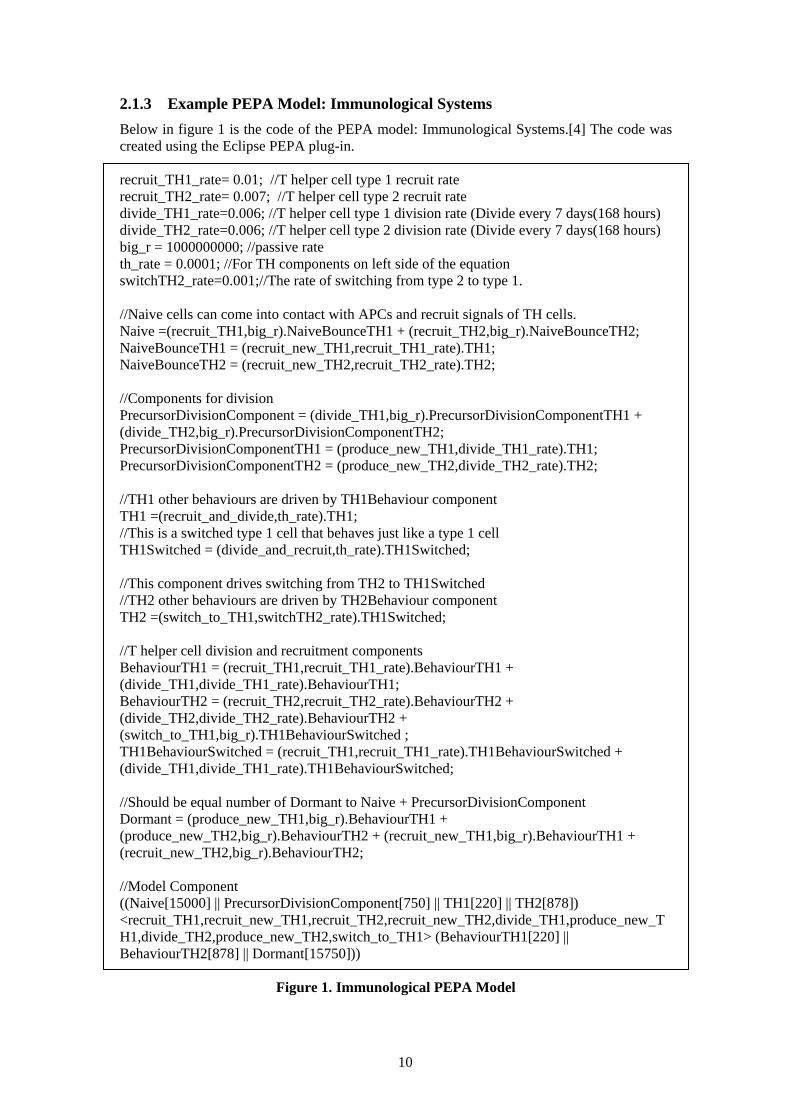
2.1.3 Example PEPA Model: Immunological Systems Below in figure 1 is the code of the PEPA model: Immunological Systems.[4] The code was created using the Eclipse PEPA plug-in. recruit_TH1_rate= 0.01; //T helper cell type 1 recruit rate recruit_TH2_rate= 0.007; //T helper cell type 2 recruit rate divide_TH1_rate=0.006; //T helper cell type 1 division rate (Divide every 7 days(168 hours) divide_TH2_rate=0.006; //T helper cell type 2 division rate (Divide every 7 days(168 hours) big_r = 1000000000; //passive rate th_rate = 0.0001; //For TH components on left side of the equation switchTH2_rate=0.001;//The rate of switching from type 2 to type 1. //Naive cells can come into contact with APCs and recruit signals of TH cells. Naive =(recruit_TH1,big_r).NaiveBounceTH1 + (recruit_TH2,big_r).NaiveBounceTH2; NaiveBounceTH1 = (recruit_new_TH1,recruit_TH1_rate).TH1; NaiveBounceTH2 = (recruit_new_TH2,recruit_TH2_rate).TH2; //Components for division PrecursorDivisionComponent = (divide_TH1,big_r).PrecursorDivisionComponentTH1 + (divide_TH2,big_r).PrecursorDivisionComponentTH2; PrecursorDivisionComponentTH1 = (produce_new_TH1,divide_TH1_rate).TH1; PrecursorDivisionComponentTH2 = (produce_new_TH2,divide_TH2_rate).TH2; //TH1 other behaviours are driven by TH1Behaviour component TH1 =(recruit_and_divide,th_rate).TH1; //This is a switched type 1 cell that behaves just like a type 1 cell TH1Switched = (divide_and_recruit,th_rate).TH1Switched; //This component drives switching from TH2 to TH1Switched //TH2 other behaviours are driven by TH2Behaviour component TH2 =(switch_to_TH1,switchTH2_rate).TH1Switched; //T helper cell division and recruitment components BehaviourTH1 = (recruit_TH1,recruit_TH1_rate).BehaviourTH1 + (divide_TH1,divide_TH1_rate).BehaviourTH1; BehaviourTH2 = (recruit_TH2,recruit_TH2_rate).BehaviourTH2 + (divide_TH2,divide_TH2_rate).BehaviourTH2 + (switch_to_TH1,big_r).TH1BehaviourSwitched ; TH1BehaviourSwitched = (recruit_TH1,recruit_TH1_rate).TH1BehaviourSwitched + (divide_TH1,divide_TH1_rate).TH1BehaviourSwitched; //Should be equal number of Dormant to Naive + PrecursorDivisionComponent Dormant = (produce_new_TH1,big_r).BehaviourTH1 + (produce_new_TH2,big_r).BehaviourTH2 + (recruit_new_TH1,big_r).BehaviourTH1 + (recruit_new_TH2,big_r).BehaviourTH2; //Model Component ((Naive[15000] || PrecursorDivisionComponent[750] || TH1[220] || TH2[878]) <recruit_TH1,recruit_new_TH1,recruit_TH2,recruit_new_TH2,divide_TH1,produce_new_TH1,divide_TH2,produce_new_TH2,switch_to_TH1> (BehaviourTH1[220] || BehaviourTH2[878] || Dormant[15750]))

Figure 1. Immunological PEPA Model

11

The problem addressed in the model is how T-helper cell populations respond to co-infections with parasites making conflicting immunological demands. This model is made up of agents which represent cells and the behaviour of the immune system. There are T helper cell agents which are either Th1 or Th2. In this model, the functions of Th1 and Th2 are not implemented: the label simply distinguishes the populations. The agents (BehaviourTH) representing Th1and Th2 have the same range of behaviour. They can recruit naive T cells to become their specific type. This behaviour is controlled by a recruitment rate which would be changed depending on the introduction of malarial infection or filarial antigen. T-helper cell agents can divide, producing new T-helper cells with the same type. The division rate is constant and set at one division per week. The Th2 cells have a further behaviour of switching. This is when the Th2 cell switches to become a Th1 cell. This behaviour is controlled by a switching rate. Additionally there are naive T cell agents with two recruitment behaviours: they either become Th1 or Th2 cells. This behaviour requires co-operation with the T-helper cell agents of that type. The model component contains all the agents and starting populations and the actions on which they synchronise. The agents on the left side of the model component synchronise on specific actions with their counterpart on the right side of the model component. The recruitment behaviour is implemented in the model using a communication bounce allowing the TH agents on the left side of the model component to be equal in population to the BehaviourTH agents on the right side of the model component. An example of this communication recruitment bounce is as follows: if a behaviour TH1 agent on the right of the model component wants to recruit a Naive agent from the left of the model component it has to synchronise on the action “recruit _ TH1”. Subsequently the Naive agent becomes a NaiveBounceTH1 agent which needs to synchronise on the action “recruit_new_TH1” with the component Dormant which is on the right side of the model component. After this action has taken place the NaiveBounceTH1 agent becomes a TH1 agent on the left side of the model component and the Dormant agent becomes BehaviourTH1 agent on the right side of the model component. The division behaviour is implemented in the same way as the recruitment behaviour above with the exception of the PrecursorDivisionComponent which acts similarly to the Naive agent in the recruitment behaviour. The switching behaviour is implemented by a synchronised action “switch_to_TH1” between the TH2 agent on the left side of the model component and the BehaviourTH2 on the right side of the model component. Subsequently the TH2 agents becomes a TH1Switched agent and the behaviour TH2 becomes a TH1BehaviourSwitched agent. Useful analysis techniques that would be carried out on this model include deriving the CTMC of this model to enable formal checking of the model and also stochastic simulations with different recruitment rates to compare with available wet lab experimental data.

2.2 Bio-PEPA (Biochemical-Performance Evaluation Process Algebra) Language

Bio-PEPA is a language for the modelling and the analysis of biochemical networks. It is based on PEPA and extends it in order to handle some features of biochemical networks, such as stoichiometry (quantity of species involved in a reaction) and the role of the species in a given reaction and different kinds of kinetic laws (different rates of reactions). The syntax is designed in order to collect the biological information needed. The syntax for terms in Bio-PEPA is defined as follows:

12

The two main components of a Bio-PEPA model are “species” components (S) which describe the behaviour of individual entities, and the model component (P), which describes the interactions between the various species. The prefix in PEPA is replaced by a new one, (α,k) op S, containing information about the role of the species in the reaction associated with α. The prefix is (α,k) where α is the action type and k is the stoichiometry coefficient of the species in that reaction. The stoichiometric coefficient captures how many molecules of a species are required for a reaction. The prefix combinator “op” represents the role of S in the action or the impact the action has on that species. The prefix combinators are: ↓ indicates a reactant, ↑ a product, an activator, an inhibitor and a generic modifier. A reactant will be consumed in the action and a product will be produced as a result of the action, activators, inhibitors and generic modifiers play a role in an action without being produced or consumed and have a defined meaning in the biochemical context. The combinators choice (+) and cooperation ( ) are as described in PEPA above. In the model component S (x) the parameter x represents the initial amount of the species. Bio-PEPA syntax also has inbuilt locations consisting of a set of species components. The prefix term (α,k) op S @ l is used to specify that the action is performed by S in location l. The notation α[I → J] S is a short hand for the pair of reactions (α,1)↓S @ I and (α,1)↑S @ J that synchronise on action α. This shorthand is very convenient when modelling agents migrating from one location to another. In Bio-PEPA functional rates are expressed explicitly for each reaction. Bio-PEPA also allows the introduction of events to the model. For example, in epidemic networks the introduction of a virus at a particular time can be described as an event. [5][6][7]

2.2.1 Bio-PEPA Analysis Techniques The Bio-PEPA language is supported by a suite of software tools which automatically process Bio-PEPA models and generate internal representation suitable for different types of analysis. These analysis techniques include: Static, Markovian, Invariant, Simulation traces and Discrete and Continuous Simulation. The Bio-PEPA plug-in utilises some of these techniques and allows the user to export appropriate file types to analyse the model in other applications.[6] Static Analysis is as in the PEPA description above with the extra detection of errors in the syntax and semantics of expressions of the kinetic laws. For example, making sure the kinetic law has the appropriate expression for inhibition if the specified action is inhibited by a defined component. Markovian Analysis: The Bio-PEPA plug-in can translate the model into a PRISM model, therefore the model’s CTMC can be analysed in the PRISM tool. PRISM is a probabilistic model checker tool. Infer Invariants analysis highlights the state and activity invariants in the model. Invariants are expressions whose value does not change during program execution. This is useful when modelling biochemical networks as some activities during reactions should remain constant. Simulation Traces can be created to export to other tools for analysis which include: Traviando, BioNessie and SBRML. Time Series Analysis is as in the PEPA description above and also within the Bio-PEPA plug-in there is a feature for experimentation, i.e. running a model with values for its parameters varying across desired ranges. [6]

13

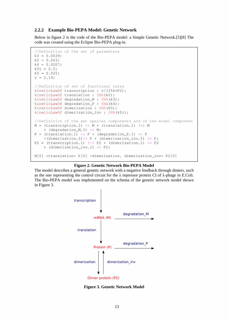
2.2.2 Example Bio-PEPA Model: Genetic Network Below in figure 2 is the code of the Bio-PEPA model: a Simple Genetic Network.[5][8] The code was created using the Eclipse Bio-PEPA plug-in. //Definition of the set of parameters k3 = 0.0039; k2 = 0.043; k4 = 0.0007; k5i = 0.5; k5 = 0.025; v = 2.19;

//Definition of set of functional rates kineticLawOf transcription : v/(356+P2); kineticLawOf translation : fMA(k2); kineticLawOf degradation_M : fMA(k3); kineticLawOf degradation_P : fMA(k4); kineticLawOf dimerization : fMA(k5); kineticLawOf dimerization_inv : fMA(k5i);

//Definition of the set species components and of the model component M = (transcription,1) >> M + (translation,1) (+) M + (degradation_M,1) << M; P = (translation,1) >> P + (degradation_P,1) << P +(dimerization,2)<< P + (dimerization_inv,2) >> P; P2 = (transcription,1) (-) P2 + (dimerization,1) >> P2 + (dimerization_inv,1) << P2;

M[0] <translation> P[0] <dimerization, dimerization_inv> P2[0]

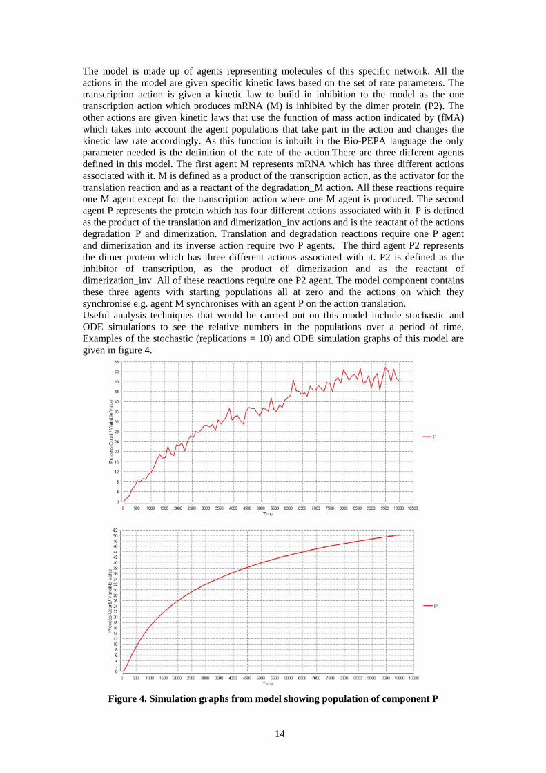
Figure 2. Genetic Network Bio-PEPA Model The model describes a general genetic network with a negative feedback through dimers, such as the one representing the control circuit for the λ repressor protein CI of λ-phage in E.Coli. The Bio-PEPA model was implemented on the schema of the genetic network model shown in Figure 3.

Figure 3. Genetic Network Model

14

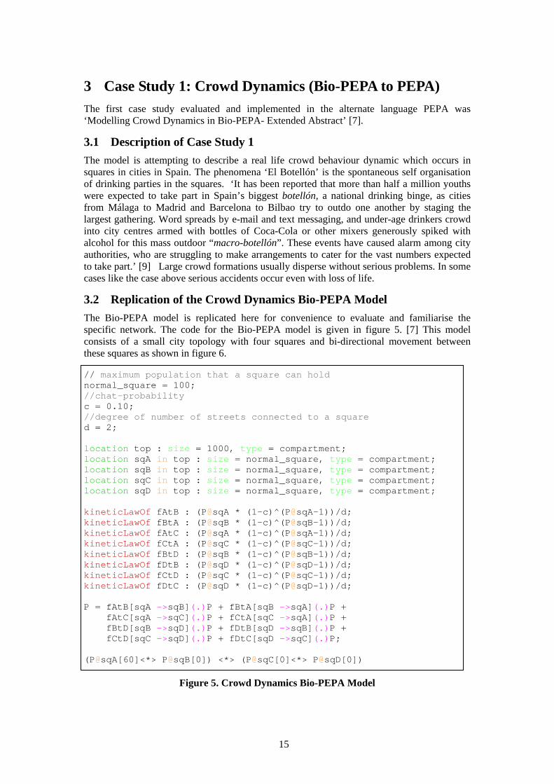
The model is made up of agents representing molecules of this specific network. All the actions in the model are given specific kinetic laws based on the set of rate parameters. The transcription action is given a kinetic law to build in inhibition to the model as the one transcription action which produces mRNA (M) is inhibited by the dimer protein (P2). The other actions are given kinetic laws that use the function of mass action indicated by (fMA) which takes into account the agent populations that take part in the action and changes the kinetic law rate accordingly. As this function is inbuilt in the Bio-PEPA language the only parameter needed is the definition of the rate of the action.There are three different agents defined in this model. The first agent M represents mRNA which has three different actions associated with it. M is defined as a product of the transcription action, as the activator for the translation reaction and as a reactant of the degradation_M action. All these reactions require one M agent except for the transcription action where one M agent is produced. The second agent P represents the protein which has four different actions associated with it. P is defined as the product of the translation and dimerization_inv actions and is the reactant of the actions degradation_P and dimerization. Translation and degradation reactions require one P agent and dimerization and its inverse action require two P agents. The third agent P2 represents the dimer protein which has three different actions associated with it. P2 is defined as the inhibitor of transcription, as the product of dimerization and as the reactant of dimerization_inv. All of these reactions require one P2 agent. The model component contains these three agents with starting populations all at zero and the actions on which they synchronise e.g. agent M synchronises with an agent P on the action translation. Useful analysis techniques that would be carried out on this model include stochastic and ODE simulations to see the relative numbers in the populations over a period of time. Examples of the stochastic (replications = 10) and ODE simulation graphs of this model are given in figure 4.

Figure 4. Simulation graphs from model showing population of component P

15

3 Case Study 1: Crowd Dynamics (Bio-PEPA to PEPA) The first case study evaluated and implemented in the alternate language PEPA was ‘Modelling Crowd Dynamics in Bio-PEPA- Extended Abstract’ [7].

3.1 Description of Case Study 1 The model is attempting to describe a real life crowd behaviour dynamic which occurs in squares in cities in Spain. The phenomena ‘El Botellón’ is the spontaneous self organisation of drinking parties in the squares. ‘It has been reported that more than half a million youths were expected to take part in Spain’s biggest botellón, a national drinking binge, as cities from Málaga to Madrid and Barcelona to Bilbao try to outdo one another by staging the largest gathering. Word spreads by e-mail and text messaging, and under-age drinkers crowd into city centres armed with bottles of Coca-Cola or other mixers generously spiked with alcohol for this mass outdoor “macro-botellón”. These events have caused alarm among city authorities, who are struggling to make arrangements to cater for the vast numbers expected to take part.’ [9] Large crowd formations usually disperse without serious problems. In some cases like the case above serious accidents occur even with loss of life.

3.2 Replication of the Crowd Dynamics Bio-PEPA Model The Bio-PEPA model is replicated here for convenience to evaluate and familiarise the specific network. The code for the Bio-PEPA model is given in figure 5. [7] This model consists of a small city topology with four squares and bi-directional movement between these squares as shown in figure 6. // maximum population that a square can hold normal_square = 100; //chat-probability c = 0.10; //degree of number of streets connected to a square d = 2;

location top : size = 1000, type = compartment; location sqA in top : size = normal_square, type = compartment; location sqB in top : size = normal_square, type = compartment; location sqC in top : size = normal_square, type = compartment; location sqD in top : size = normal_square, type = compartment;

kineticLawOf fAtB : (P@sqA * (1-c)^(P@sqA-1))/d; kineticLawOf fBtA : (P@sqB * (1-c)^(P@sqB-1))/d; kineticLawOf fAtC : (P@sqA * (1-c)^(P@sqA-1))/d; kineticLawOf fCtA : (P@sqC * (1-c)^(P@sqC-1))/d; kineticLawOf fBtD : (P@sqB * (1-c)^(P@sqB-1))/d; kineticLawOf fDtB : (P@sqD * (1-c)^(P@sqD-1))/d; kineticLawOf fCtD : (P@sqC * (1-c)^(P@sqC-1))/d; kineticLawOf fDtC : (P@sqD * (1-c)^(P@sqD-1))/d;

P = fAtB[sqA ->sqB](.)P + fBtA[sqB ->sqA](.)P + fAtC[sqA ->sqC](.)P + fCtA[sqC ->sqA](.)P + fBtD[sqB ->sqD](.)P + fDtB[sqD ->sqB](.)P + fCtD[sqC ->sqD](.)P + fDtC[sqD ->sqC](.)P;

(P@sqA[60]<*> P@sqB[0]) <*> (P@sqC[0]<*> P@sqD[0])

Figure 5. Crowd Dynamics Bio-PEPA Model

16

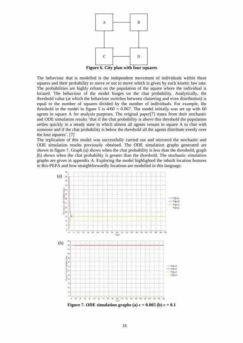
Figure 6. City plan with four squares The behaviour that is modelled is the independent movement of individuals within these squares and their probability to move or not to move which is given by each kinetic law rate. The probabilities are highly reliant on the population of the square where the individual is located. The behaviour of the model hinges on the chat probability. Analytically, the threshold value (at which the behaviour switches between clustering and even distribution) is equal to the number of squares divided by the number of individuals. For example, the threshold in the model in figure 5 is 4/60 = 0.067. The model initially was set up with 60 agents in square A for analysis purposes. The original paper[7] states from their stochastic and ODE simulation results ‘that if the chat probability is above this threshold the population settles quickly in a steady state in which almost all agents remain in square A to chat with someone and if the chat probability is below the threshold all the agents distribute evenly over the four squares’. [7] The replication of this model was successfully carried out and mirrored the stochastic and ODE simulation results previously obtained. The ODE simulation graphs generated are shown in figure 7. Graph (a) shows when the chat probability is less than the threshold; graph (b) shows when the chat probability is greater than the threshold. The stochastic simulation graphs are given in appendix A. Exploring the model highlighted the inbuilt location features in Bio-PEPA and how straightforwardly locations are modelled in this language. (a) (b)

Figure 7. ODE simulation graphs (a) c = 0.005 (b) c = 0.1

17

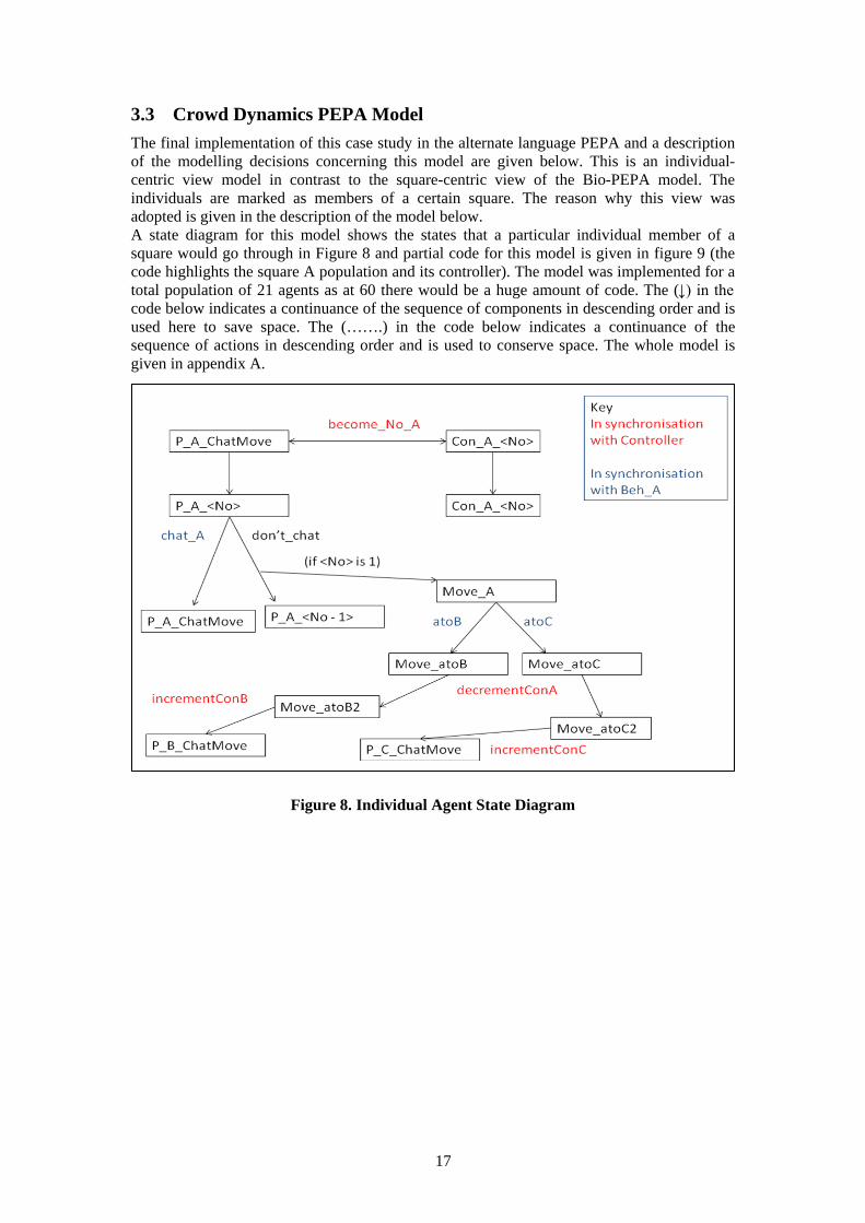
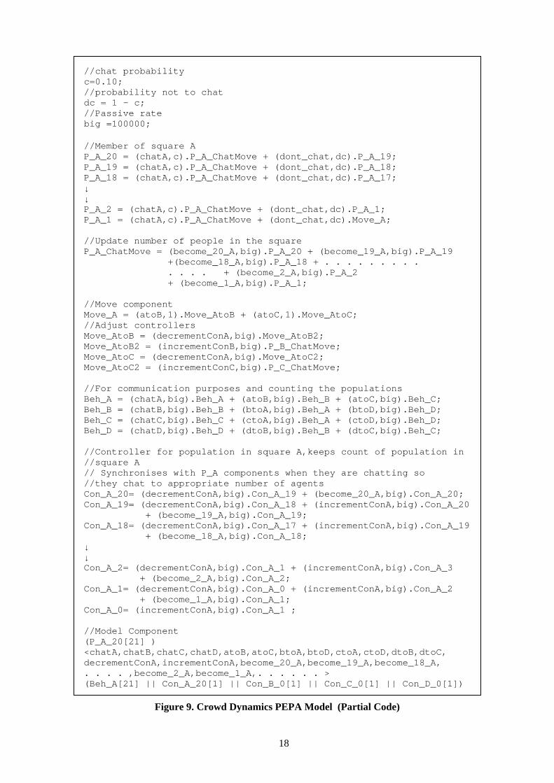
3.3 Crowd Dynamics PEPA Model The final implementation of this case study in the alternate language PEPA and a description of the modelling decisions concerning this model are given below. This is an individual- centric view model in contrast to the square-centric view of the Bio-PEPA model. The individuals are marked as members of a certain square. The reason why this view was adopted is given in the description of the model below. A state diagram for this model shows the states that a particular individual member of a square would go through in Figure 8 and partial code for this model is given in figure 9 (the code highlights the square A population and its controller). The model was implemented for a total population of 21 agents as at 60 there would be a huge amount of code. The (↓) in the code below indicates a continuance of the sequence of components in descending order and is used here to save space. The (…….) in the code below indicates a continuance of the sequence of actions in descending order and is used to conserve space. The whole model is given in appendix A.

Figure 8. Individual Agent State Diagram

18

//chat probability c=0.10; //probability not to chat dc = 1 - c; //Passive rate big =100000; //Member of square A P_A_20 = (chatA,c).P_A_ChatMove + (dont_chat,dc).P_A_19; P_A_19 = (chatA,c).P_A_ChatMove + (dont_chat,dc).P_A_18; P_A_18 = (chatA,c).P_A_ChatMove + (dont_chat,dc).P_A_17; ↓ ↓ P_A_2 = (chatA,c).P_A_ChatMove + (dont_chat,dc).P_A_1; P_A_1 = (chatA,c).P_A_ChatMove + (dont_chat,dc).Move_A; //Update number of people in the square P_A_ChatMove = (become_20_A,big).P_A_20 + (become_19_A,big).P_A_19 +(become_18_A,big).P_A_18 + . . . . . . . . . . . . . + (become_2_A,big).P_A_2 + (become_1_A,big).P_A_1; //Move component Move_A = (atoB,1).Move_AtoB + (atoC,1).Move_AtoC; //Adjust controllers Move_AtoB = (decrementConA,big).Move_AtoB2; Move_AtoB2 = (incrementConB,big).P_B_ChatMove; Move_AtoC = (decrementConA,big).Move_AtoC2; Move_AtoC2 = (incrementConC,big).P_C_ChatMove; //For communication purposes and counting the populations Beh_A = (chatA,big).Beh_A + (atoB,big).Beh_B + (atoC,big).Beh_C; Beh_B = (chatB,big).Beh_B + (btoA,big).Beh_A + (btoD,big).Beh_D; Beh_C = (chatC,big).Beh_C + (ctoA,big).Beh_A + (ctoD,big).Beh_D; Beh_D = (chatD,big).Beh_D + (dtoB,big).Beh_B + (dtoC,big).Beh_C; //Controller for population in square A,keeps count of population in //square A // Synchronises with P_A components when they are chatting so //they chat to appropriate number of agents Con_A_20= (decrementConA,big).Con_A_19 + (become_20_A,big).Con_A_20; Con_A_19= (decrementConA,big).Con_A_18 + (incrementConA,big).Con_A_20 + (become_19_A,big).Con_A_19; Con_A_18= (decrementConA,big).Con_A_17 + (incrementConA,big).Con_A_19 + (become_18_A,big).Con_A_18; ↓ ↓ Con_A_2= (decrementConA,big).Con_A_1 + (incrementConA,big).Con_A_3 + (become_2_A,big).Con_A_2; Con_A_1= (decrementConA,big).Con_A_0 + (incrementConA,big).Con_A_2 + (become_1_A,big).Con_A_1; Con_A_0= (incrementConA,big).Con_A_1 ; //Model Component (P_A_20[21] ) <chatA,chatB,chatC,chatD,atoB,atoC,btoA,btoD,ctoA,ctoD,dtoB,dtoC, decrementConA,incrementConA,become_20_A,become_19_A,become_18_A, . . . . ,become_2_A,become_1_A,. . . . . . > (Beh_A[21] || Con_A_20[1] || Con_B_0[1] || Con_C_0[1] || Con_D_0[1])

Figure 9. Crowd Dynamics PEPA Model (Partial Code)

19

3.3.1 Description of PEPA Model Four issues will be discussed to evaluate why the final model is structured in this way. Firstly, why this model is not implemented in a square centric view and is implemented in an individual centric view. Secondly, describing how the agents communicate in the same square population. Thirdly, describing how the mechanism of an agent moving from one square to another was implemented and issues that arose from this. Fourthly, describing how these issues were overcome by using controller mechanisms.

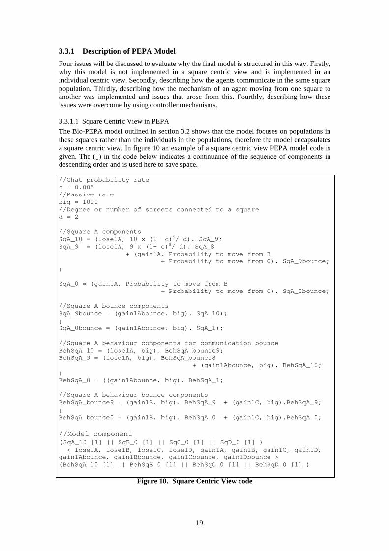
3.3.1.1 Square Centric View in PEPA The Bio-PEPA model outlined in section 3.2 shows that the model focuses on populations in these squares rather than the individuals in the populations, therefore the model encapsulates a square centric view. In figure 10 an example of a square centric view PEPA model code is given. The (↓) in the code below indicates a continuance of the sequence of components in descending order and is used here to save space. //Chat probability rate c = 0.005 //Passive rate big = 1000 //Degree or number of streets connected to a square d = 2 //Square A components SqA_10 = (lose1A, 10 x (1- c)9/ d). SqA_9; SqA_9 = (lose1A, 9 x (1- c)8/ d). SqA_8 + (gain1A, Probability to move from B + Probability to move from C). SqA_9bounce; ↓ SqA_0 = (gain1A, Probability to move from B + Probability to move from C). SqA_0bounce; //Square A bounce components SqA_9bounce = (gain1Abounce, big). SqA_10); ↓ SqA_0bounce = (gain1Abounce, big). SqA_1); //Square A behaviour components for communication bounce BehSqA_10 = (lose1A, big). BehSqA_bounce9; BehSqA_9 = (lose1A, big). BehSqA_bounce8 + (gain1Abounce, big). BehSqA_10; ↓ BehSqA_0 = ((gain1Abounce, big). BehSqA_1; //Square A behaviour bounce components BehSqA_bounce9 = (gain1B, big). BehSqA_9 + (gain1C, big).BehSqA_9; ↓ BehSqA_bounce0 = (gain1B, big). BehSqA_0 + (gain1C, big).BehSqA_0; //Model component (SqA_10 [1] || SqB_0 [1] || SqC_0 [1] || SqD_0 [1] ) < lose1A, lose1B, lose1C, lose1D, gain1A, gain1B, gain1C, gain1D, gain1Abounce, gain1Bbounce, gain1Cbounce, gain1Dbounce > (BehSqA_10 [1] || BehSqB_0 [1] || BehSqC_0 [1] || BehSqD_0 [1] )

Figure 10. Square Centric View code

20

In the model above the population of the square is coded as part of the component name, as PEPA does not have the inbuilt location feature to assign these components squares certain starting population values. The model contains behaviour bounce components which are required for the squares to synchronise and update their relative populations according to the actions that are carried out in specific squares. For example, if SqA_10 carries out the action “lose1A” it becomes SqA_9 it needs to synchronise on this action with “BehSqA_10”, subsequently this behaviour component becomes BehSqA_bounce9 which synchronises on the action “gain1B” with the component SqB_9. This Component SqB_9 becomes SqB_9bounce which synchronises on the action “gain1Bbounce” with the component BehSqB_9. Therefore, the behaviour component becomes equal to BehSqB_10 and component becomes equal to SqB_10. The behaviour components should always be equal to the components. Implementing the PEPA model in this square centric way cannot and does not produce the desired behaviour. Firstly it would be difficult if not impossible to construct a square centric view model because multiple calculations in rates would be required for each individual square and its subsequent states. For example, for a square to gain one agent (gain1 action) the probability of an individual moving from two other squares requires to be calculated to give the rate of the action and this rate would change as the movement occurs; therefore, this rate would require to be changed constantly. Secondly to observe individual behaviour the model would require to encapsulate individual agents and their actions. This is a more relevant and natural PEPA style of coding. Therefore, the resulting model is focused on an individual centric view rather than the square centric view.

3.3.1.2 Communication between Members of the Same Square One part of the behaviour of the model was the communication between members of the same square to perform the chat activity. This was implemented by creating behaviour components for each square population. In the model component these behaviour components are placed on the right side of the cooperation combinator and the member agents are placed on the left. Therefore this behaviour component gives a communication bounce back mechanism enabling members of the same square to synchronise on a chat action “chat_A”. This synchronisation behaviour with behaviour components is shown in the state diagram in blue in figure 8.

3.3.1.3 Independent choice mechanism of an agent moving from one square to another The first development of the independent choice of an individual wishing to leave a square was implemented by a “don’t chat” action with a rate of the inverse of the chat action probability. The model code for this first development is given in figure 11. Therefore, an individual in this model has a choice of two actions either to chat or not to chat. If the individual action “don’t chat” is taken the individual agent becomes a move component agent where they have an equal independent choice to become a member of a square (two available) that is connected to their current square. The action to move to a different square is synchronised with the behaviour component therefore the populations of member agents and behaviour components remain equal. Stochastic and ODE simulation analysis was carried out on this first development with a starting population of 60 in square A with the chat probability at 0.005(below the analytical threshold) and 0.1(above the analytical threshold). The stochastic simulation graphs with chat probability at 0.005 (a) and 0.1(b) are given in figure 12. Analysis of these simulations found that the agents freely move between squares for either of these chat probabilities, even at the chat probability 0.99 the agents still slowly distribute between the squares. This indicated that the “don’t chat” action had a huge pull against the chat action and the model was not reacting to the relationship between the population numbers of a square and the chat action probability rate. This was confirmed by looking at the kinetic rates which PEPA creates for the model which gave the kinetic rate of (dc.P_A) for the “don’t chat” action which is not the desired kinetic rate that is seen in the Bio-PEPA model which is ((P@sqA * (1-c)^(P@sqA-1))/d).

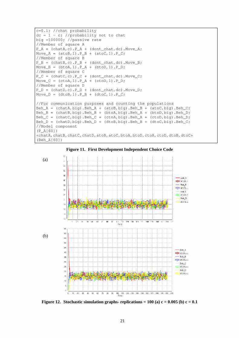
21

c=0.1; //chat probability dc = 1 - c; //probability not to chat big =100000; //passive rate //Member of square A P_A = (chatA,c).P_A + (dont_chat,dc).Move_A; Move_A = (atoB,1).P_B + (atoC,1).P_C; //Member of square B P_B = (chatB,c).P_B + (dont_chat,dc).Move_B; Move_B = (btoA,1).P_A + (btoD,1).P_D; //Member of square C P_C = (chatC,c).P_C + (dont_chat,dc).Move_C; Move_C = (ctoA,1).P_A + (ctoD,1).P_D; //Member of square D P_D = (chatD,c).P_D + (dont_chat,dc).Move_D; Move_D = (dtoB,1).P_B + (dtoC,1).P_C;

//For communication purposes and counting the populations Beh_A = (chatA,big).Beh_A + (atoB,big).Beh_B + (atoC,big).Beh_C; Beh_B = (chatB,big).Beh_B + (btoA,big).Beh_A + (btoD,big).Beh_D; Beh_C = (chatC,big).Beh_C + (ctoA,big).Beh_A + (ctoD,big).Beh_D; Beh_D = (chatD,big).Beh_D + (dtoB,big).Beh_B + (dtoC,big).Beh_C; //Model component (P_A[60]) <chatA,chatB,chatC,chatD,atoB,atoC,btoA,btoD,ctoA,ctoD,dtoB,dtoC> (Beh_A[60])

Figure 11. First Development Independent Choice Code

(a) (b)

Figure 12. Stochastic simulation graphs- replications = 100 (a) c = 0.005 (b) c = 0.1

22

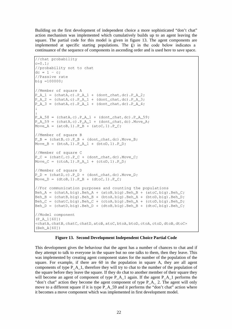
Building on the first development of independent choice a more sophisticated “don’t chat” action mechanism was implemented which cumulatively builds up to an agent leaving the square. The partial code for this model is given in figure 13. The agent components are implemented at specific starting populations. The (↓) in the code below indicates a continuance of the sequence of components in ascending order and is used here to save space. //chat probability c=0.1; //probability not to chat dc = 1 - c; //Passive rate big =100000; //Member of square A P_A_1 = (chatA,c).P_A_1 + (dont_chat,dc).P_A_2; P_A_2 = (chatA,c).P_A_1 + (dont_chat,dc).P_A_3; P_A_3 = (chatA,c).P_A_1 + (dont_chat,dc).P_A_4; ↓ ↓ P_A_58 = (chatA,c).P_A_1 + (dont_chat,dc).P_A_59; P_A_59 = (chatA,c).P_A_1 + (dont_chat,dc).Move_A; Move_A = (atoB,1).P_B + (atoC,1).P_C; //Member of square B P_B = (chatB,c).P_B + (dont_chat,dc).Move_B; Move_B = (btoA,1).P_A_1 + (btoD,1).P_D; //Member of square C P_C = (chatC,c).P_C + (dont_chat,dc).Move_C; Move_C = (ctoA,1).P_A_1 + (ctoD,1).P_D; //Member of square D P_D = (chatD,c).P_D + (dont_chat,dc).Move_D; Move_D = (dtoB,1).P_B + (dtoC,1).P_C; //For communication purposes and counting the populations Beh_A = (chatA,big).Beh_A + (atoB,big).Beh_B + (atoC,big).Beh_C; Beh_B = (chatB,big).Beh_B + (btoA,big).Beh_A + (btoD,big).Beh_D; Beh_C = (chatC,big).Beh_C + (ctoA,big).Beh_A + (ctoD,big).Beh_D; Beh_D = (chatD,big).Beh_D + (dtoB,big).Beh_B + (dtoC,big).Beh_C; //Model component (P_A_1[60]) <chatA,chatB,chatC,chatD,atoB,atoC,btoA,btoD,ctoA,ctoD,dtoB,dtoC> (Beh_A[60])

Figure 13. Second Development Independent Choice Partial Code

This development gives the behaviour that the agent has a number of chances to chat and if they attempt to talk to everyone in the square but no one talks to them, then they leave. This was implemented by creating agent component states for the number of the population of the square. For example, if there are 60 in the population in square A, they are all agent components of type P_A_1, therefore they will try to chat to the number of the population of the square before they leave the square. If they do chat to another member of their square they will become an agent of component of type P_A_1 again. If the agent P_A_1 performs the “don’t chat” action they become the agent component of type P_A_ 2. The agent will only move to a different square if it is type P_A_59 and it performs the “don’t chat” action where it becomes a move component which was implemented in first development model.

23

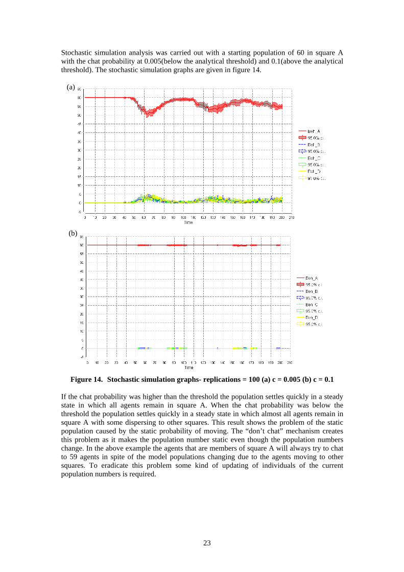
Stochastic simulation analysis was carried out with a starting population of 60 in square A with the chat probability at 0.005(below the analytical threshold) and 0.1(above the analytical threshold). The stochastic simulation graphs are given in figure 14.

(a) (b)

Figure 14. Stochastic simulation graphs- replications = 100 (a) c = 0.005 (b) c = 0.1 If the chat probability was higher than the threshold the population settles quickly in a steady state in which all agents remain in square A. When the chat probability was below the threshold the population settles quickly in a steady state in which almost all agents remain in square A with some dispersing to other squares. This result shows the problem of the static population caused by the static probability of moving. The “don’t chat” mechanism creates this problem as it makes the population number static even though the population numbers change. In the above example the agents that are members of square A will always try to chat to 59 agents in spite of the model populations changing due to the agents moving to other squares. To eradicate this problem some kind of updating of individuals of the current population numbers is required.

24

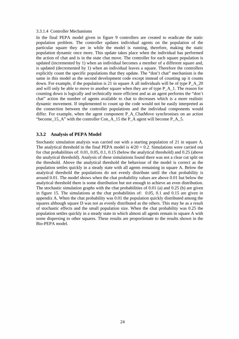
3.3.1.4 Controller Mechanisms In the final PEPA model given in figure 9 controllers are created to eradicate the static population problem. The controller updates individual agents on the population of the particular square they are in while the model is running, therefore, making the static population dynamic once more. This update takes place when the individual has performed the action of chat and is in the state chat move. The controller for each square population is updated (incremented by 1) when an individual becomes a member of a different square and, is updated (decremented by 1) when an individual leaves a square. Therefore the controllers explicitly count the specific populations that they update. The “don’t chat” mechanism is the same in this model as the second development code except instead of counting up it counts down. For example, if the population is 21 in square A all individuals will be of type P_A_20 and will only be able to move to another square when they are of type P_A_1. The reason for counting down is logically and technically more efficient and as an agent performs the “don’t chat” action the number of agents available to chat to decreases which is a more realistic dynamic movement. If implemented to count up the code would not be easily interpreted as the connection between the controller populations and the individual components would differ. For example, when the agent component P_A_ChatMove synchronises on an action “become_15_A” with the controller Con_A_15 the P_A agent will become P_A_5.

3.3.2 Analysis of PEPA Model Stochastic simulation analysis was carried out with a starting population of 21 in square A. The analytical threshold in the final PEPA model is 4/20 = 0.2. Simulations were carried out for chat probabilities of: 0.01, 0.05, 0.1, 0.15 (below the analytical threshold) and 0.25 (above the analytical threshold). Analysis of these simulations found there was not a clear cut split on the threshold. Above the analytical threshold the behaviour of the model is correct as the population settles quickly in a steady state with all agents remaining in square A. Below the analytical threshold the populations do not evenly distribute until the chat probability is around 0.01. The model shows when the chat probability values are above 0.01 but below the analytical threshold there is some distribution but not enough to achieve an even distribution. The stochastic simulation graphs with the chat probabilities of 0.01 (a) and 0.25 (b) are given in figure 15. The simulations at the chat probabilities of: 0.05, 0.1 and 0.15 are given in appendix A. When the chat probability was 0.01 the population quickly distributed among the squares although square D was not as evenly distributed as the others. This may be as a result of stochastic effects and the small population size. When the chat probability was 0.25 the population settles quickly in a steady state in which almost all agents remain in square A with some dispersing to other squares. These results are proportionate to the results shown in the Bio-PEPA model.

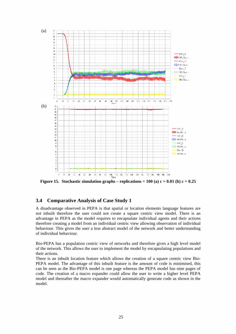
25

(a)

(b)

Figure 15. Stochastic simulation graphs – replications = 100 (a) c = 0.01 (b) c = 0.25

3.4 Comparative Analysis of Case Study 1 A disadvantage observed in PEPA is that spatial or location elements language features are not inbuilt therefore the user could not create a square centric view model. There is an advantage in PEPA as the model requires to encapsulate individual agents and their actions therefore creating a model from an individual centric view allowing observation of individual behaviour. This gives the user a less abstract model of the network and better understanding of individual behaviour. Bio-PEPA has a population centric view of networks and therefore gives a high level model of the network. This allows the user to implement the model by encapsulating populations and their actions. There is an inbuilt location feature which allows the creation of a square centric view Bio-PEPA model. The advantage of this inbuilt feature is the amount of code is minimised, this can be seen as the Bio-PEPA model is one page whereas the PEPA model has nine pages of code. The creation of a macro expander could allow the user to write a higher level PEPA model and thereafter the macro expander would automatically generate code as shown in the model.

26

A disadvantage observed in Bio-PEPA is the manual creation of kinetic laws for each action, for example, for an agent to stay or leave a square. The user has to be particularly careful to create the correct kinetic laws to create the correct system behaviour. An advantage in PEPA is that the creation of the kinetic laws are automatically generated by PEPA, therefore the user can concentrate on building the model to simulate the correct behaviour of the specific network; although, building the model is not particularly straightforward. An advantage observed in Bio-PEPA of having manual kinetic laws is that the user can immediately introduce the influence specific populations have with the rates of specific actions. For example, the probability rates of staying and chatting and not chatting and leaving will be influenced by the number of the population within each square. A disadvantage observed in PEPA automatically generating the kinetic laws is they may not be what the user intended or what the user thinks they are. For example in first development of the independent choice to leave a square, the kinetic law for the “don’t chat” action was not what was intended. To change the kinetic laws that PEPA creates the model needs implementation of mechanisms. For example, more sophisticated “don’t chat” action mechanism which cumulatively builds up to an agent leaving the square. A disadvantage observed concerning the creation of these mechanisms was the populations became static and therefore analysis of the model gave incorrect results. To overcome these problem controllers were implemented to make the populations dynamic. Having these mechanism and controllers in the model made the model complex and also certain analysis techniques such as ODE simulation became unsuitable to analyse the model because ODE derivation relies on many copies of the same component and this model did not comply with this. Changing the starting populations in the model also is complex if not near impossible therefore making it hard to analyse the network in different ways. An advantage observed in Bio-PEPA was the changing of starting populations is relatively straight forward to further analyse the model. To conclude, PEPA is useful to begin with to obtain an understanding of the individual agents and their actions in this crowd dynamic model. To be able to carry out more analysis on the overall system it is more straightforward to implement models in Bio-PEPA because of its inbuilt location language feature. If locations and spatial elements are of a high requirement in the model, the language recommended to use is Bio-PEPA.

27

4 Case Study 2: Immunological Systems (PEPA to Bio-PEPA)

The second case study evaluated and implemented in the alternate language Bio-PEPA was ‘Modelling Immunological Systems using PEPA: a preliminary report’.[4]

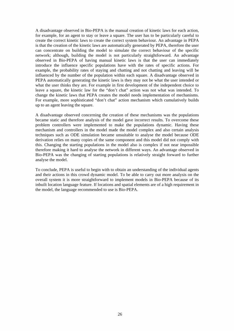
4.1 Description of Case Study 2 The problem addressed in the model is how T-helper cell populations respond to co-infections with parasites making conflicting immunological demands. The model focuses on the populations of T-helper Th1 and Th2 cell types. These cells differ in their pattern of cytokine secretion. Functionally the molecules secreted by Th1 cells lead to cell mediated and inflammatory immune responses, while those secreted by Th2 cells intervene in humoral immune responses. Importantly, cytokines (IFN & IL4) produced by Th cells promote the recruitment of naive cells (Th0) to become their specific type of Th cell either Th1 or Th2, and at the same time inhibit the recruitment of each other. Figure 16 shows this recruitment behaviour. The resulting activatory and inhibitory cross-regulations create a complex network at the molecular and cellular levels.[15]

Figure 16. Recruitment of Naïve Th cells [15] The co-infections investigated in the model were malaria (microbial infection) and helminth (micro parasite infection). Malaria is caused by a parasite known as plasmodium. When the parasite enters the blood through a bite from a mosquito, it travels straight to the liver. It develops there and then re-enters the bloodstream and invades the red blood cells. Once in the red blood cells, the parasites grow and multiply. Eventually, the infected red blood cells burst and release even more parasites into the blood. The infected cells usually burst every 48-72 hours. Each time this happens, the host will experience an attack of chills, fever and sweating.[16] The control of Microbial infections depends on the presence of Th1 cell types. Derived from the Greek word “helmins,” meaning “worm,” Helminth is a broad categorical term referring to various types of parasitic worms that reside in the body. The Helminth eggs enter the human body usually through three transmission routes: the mouth, nose, or anus. Parasites get their nourishment from their hosts, causing disease and sickness while continuing to feed off of their environment. The most common symptoms of helminth infections and intestinal worms include diarrhoea, foul breath, headaches, nausea, abdominal pain, and itching.[17] The control of helminth infections depends on the presence of Th2 cell types. These contrasting immune responses can interact in helminth-micro parasite co-infection and can affect severity and the outcome of disease.

28

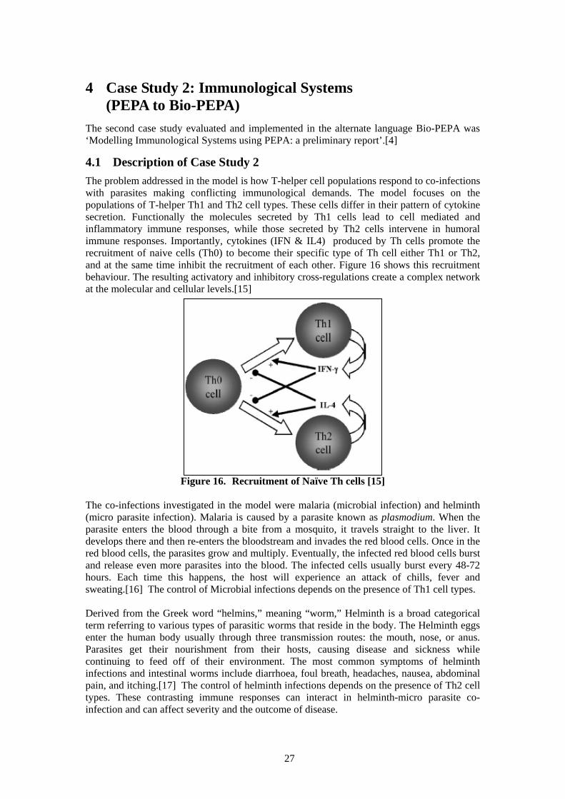
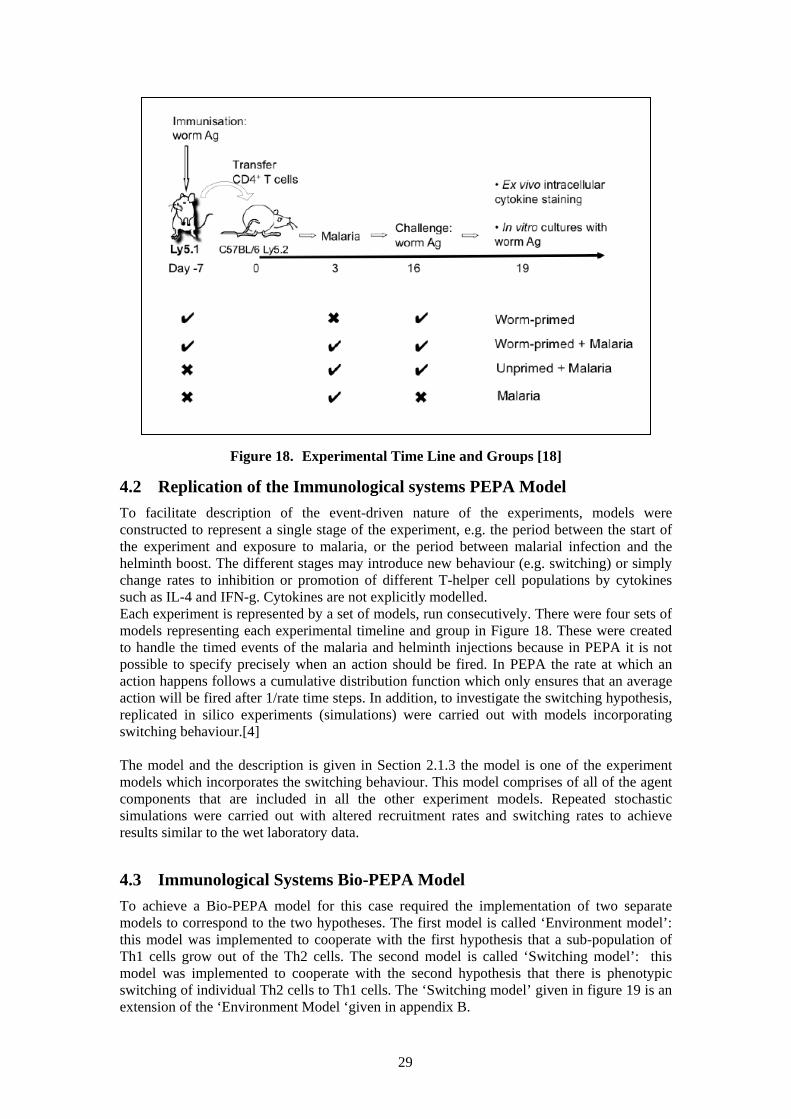
The model was implemented to investigate two alternative hypotheses that were deduced from wet laboratory experimentation. Figure 18 shows the experimental design, with timeline, and with variants to expose the behaviour of the Th1 and Th2 populations. Experimental results show there is a switch from Th2 to Th1 cytokine profiles. Figure 17 gives an indication of Th1 population sizes (defined by production of the cytokine interferon (IFN)-g) on the left, with Th2 population sizes (defined by production of the cytokine interleukin (IL)-4), on the right. The graph shows multiple results for different filarial antigen. Points indicate particular results, and the lines are the average results. It was noted that in mice exposed to malaria infections the level of Th2 falls while the Th1 population increases compared to mice injected with worm antigen only. It is not known how this change occurs, and therefore two alternate hypotheses were formed. The first hypothesis is that a sub-population of Th1 cells grow out of the Th2 cells. The second hypothesis is that there is phenotypic switching of individual Th2 cells to Th1 cells.[4] [18]

Figure 17. Experimental Results Th1 Population (left) , Th2 Population (right)[18]

29

Figure 18. Experimental Time Line and Groups [18]

4.2 Replication of the Immunological systems PEPA Model To facilitate description of the event-driven nature of the experiments, models were constructed to represent a single stage of the experiment, e.g. the period between the start of the experiment and exposure to malaria, or the period between malarial infection and the helminth boost. The different stages may introduce new behaviour (e.g. switching) or simply change rates to inhibition or promotion of different T-helper cell populations by cytokines such as IL-4 and IFN-g. Cytokines are not explicitly modelled. Each experiment is represented by a set of models, run consecutively. There were four sets of models representing each experimental timeline and group in Figure 18. These were created to handle the timed events of the malaria and helminth injections because in PEPA it is not possible to specify precisely when an action should be fired. In PEPA the rate at which an action happens follows a cumulative distribution function which only ensures that an average action will be fired after 1/rate time steps. In addition, to investigate the switching hypothesis, replicated in silico experiments (simulations) were carried out with models incorporating switching behaviour.[4] The model and the description is given in Section 2.1.3 the model is one of the experiment models which incorporates the switching behaviour. This model comprises of all of the agent components that are included in all the other experiment models. Repeated stochastic simulations were carried out with altered recruitment rates and switching rates to achieve results similar to the wet laboratory data.

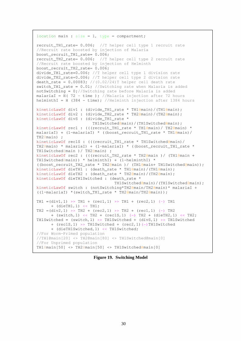
4.3 Immunological Systems Bio-PEPA Model To achieve a Bio-PEPA model for this case required the implementation of two separate models to correspond to the two hypotheses. The first model is called ‘Environment model’: this model was implemented to cooperate with the first hypothesis that a sub-population of Th1 cells grow out of the Th2 cells. The second model is called ‘Switching model’: this model was implemented to cooperate with the second hypothesis that there is phenotypic switching of individual Th2 cells to Th1 cells. The ‘Switching model’ given in figure 19 is an extension of the ‘Environment Model ‘given in appendix B.

30

location main : size = 1, type = compartment; recruit_TH1_rate= 0.006; //T helper cell type 1 recruit rate //Recruit rate boosted by injection of Malaria boost_recruit_TH1_rate= 0.006; recruit_TH2_rate= 0.006; //T helper cell type 2 recruit rate //Recruit rate boosted by injection of Helminth boost_recruit_TH2_rate= 0.006; divide_TH1_rate=0.006; //T helper cell type 1 division rate divide_TH2_rate=0.006; //T helper cell type 2 division rate death_rate = 0.00083; //(0.02/24)T helper cell death rate switch_TH1_rate = 0.01; //Switching rate when Malaria is added notSwitching = 0;//Switching rate before Malaria is added malariaI = H( 72 - time ); //Malaria injection after 72 hours helminthI = H (384 - time); //Helminth injection after 1384 hours kineticLawOf div1 : (divide_TH1_rate * TH1@main)/(TH1@main); kineticLawOf div2 : (divide_TH2_rate * TH2@main)/(TH2@main); kineticLawOf divS : (divide_TH1_rate * TH1Switched@main)/(TH1Switched@main); kineticLawOf rec1 : (((recruit_TH1_rate * TH1@main)/ TH2@main) * malariaI) + (1-malariaI) * ((boost_recruit_TH1_rate * TH1@main)/ TH2@main) ; kineticLawOf rec1S : (((recruit_TH1_rate * TH1Switched@main)/ TH2@main) * malariaI) + (1-malariaI) * ((boost_recruit_TH1_rate * TH1Switched@main )/ TH2@main) ; kineticLawOf rec2 : (((recruit_TH2_rate * TH2@main )/ (TH1@main + TH1Switched@main)) * helminthI) + (1-helminthI) * ((boost_recruit_TH2_rate * TH2@main )/ (TH1@main+ TH1Switched@main)); kineticLawOf dieTH1 : (death_rate * TH1@main)/(TH1@main); kineticLawOf dieTH2 : (death_rate * TH2@main)/(TH2@main); kineticLawOf dieTH1Switched : (death_rate * TH1Switched@main)/(TH1Switched@main); kineticLawOf switch : (notSwitching*TH2@main/TH2@main)* malariaI + ((1-malariaI) *(switch_TH1_rate * TH2@main/TH2@main)); TH1 =(div1,1) >> TH1 + (rec1,1) >> TH1 + (rec2,1) (-) TH1 + (dieTH1,1) << TH1; TH2 =(div2,1) >> TH2 + (rec2,1) >> TH2 + (rec1,1) (-) TH2 + (switch,1) << TH2 + (rec1S,1) (-) TH2 + (dieTH2,1) << TH2; TH1Switched = (switch,1) >> TH1Switched + (divS,1) >> TH1Switched + (rec1S,1) >> TH1Switched + (rec2,1)(-)TH1Switched + (dieTH1Switched,1) << TH1Switched; //For Worm-Primed population //TH1@main[20] <> TH2@main[80] <> TH1Switched@main[0] //For Unprimed population TH1@main[50] <> TH2@main[50] <> TH1Switched@main[0]

Figure 19. Switching Model

31

4.3.1 Description of Bio-PEPA Models The species involved are TH1 (T helper cells of type 1) and TH2 (T helper cells of type 2) and for the switching model an extra species is added TH1Switched (Th2 cell which has switched to become Th1 cell), and the interactions are:

(i) Division of TH1 described as TH1 → 2TH1, (div1); (ii) Division of TH2 described as TH2 → 2TH2, (div2); (iii) Recruitment of TH1 described as TH1 → 2TH1, Promoted by TH1 population and

inhibited by TH2 population, (rec1); (iv) Recruitment of TH2 described as TH2 → 2TH2, Promoted by TH2 population and

inhibited by TH1 population, (rec2); (v) Both species can degrade, described as TH1 → 0 and TH2 → 0, (dieTH1,dieTH2); (vi) Switching of TH2 to become TH1 described as TH2→TH1, (switch).

The last interaction (vi) only is implemented in the switching Bio-PEPA model.

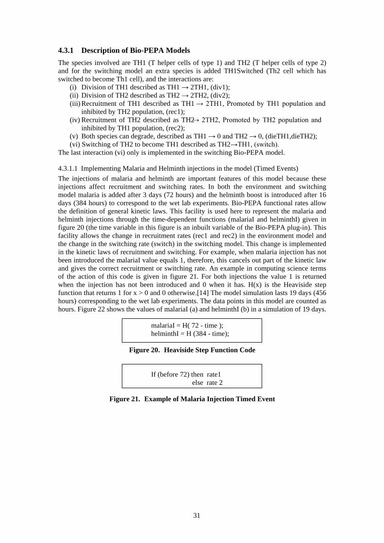
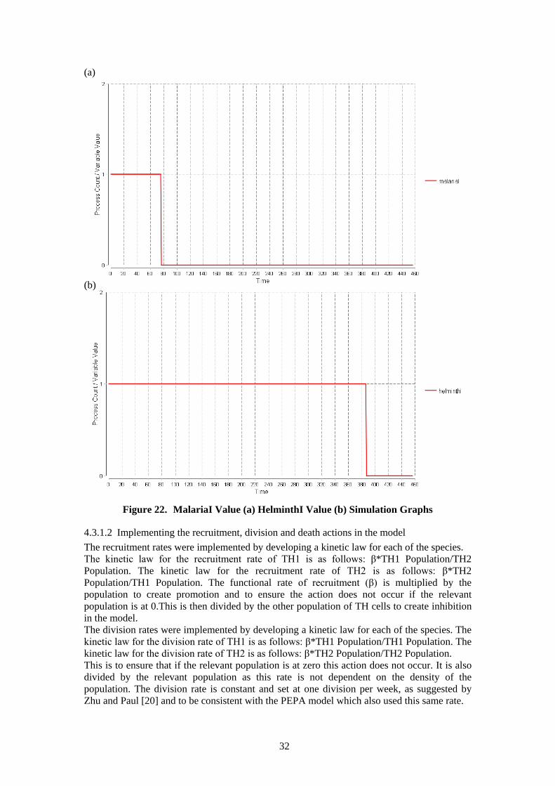
4.3.1.1 Implementing Malaria and Helminth injections in the model (Timed Events) The injections of malaria and helminth are important features of this model because these injections affect recruitment and switching rates. In both the environment and switching model malaria is added after 3 days (72 hours) and the helminth boost is introduced after 16 days (384 hours) to correspond to the wet lab experiments. Bio-PEPA functional rates allow the definition of general kinetic laws. This facility is used here to represent the malaria and helminth injections through the time-dependent functions (malariaI and helminthI) given in figure 20 (the time variable in this figure is an inbuilt variable of the Bio-PEPA plug-in). This facility allows the change in recruitment rates (rec1 and rec2) in the environment model and the change in the switching rate (switch) in the switching model. This change is implemented in the kinetic laws of recruitment and switching. For example, when malaria injection has not been introduced the malariaI value equals 1, therefore, this cancels out part of the kinetic law and gives the correct recruitment or switching rate. An example in computing science terms of the action of this code is given in figure 21. For both injections the value 1 is returned when the injection has not been introduced and 0 when it has. H(x) is the Heaviside step function that returns 1 for x > 0 and 0 otherwise.[14] The model simulation lasts 19 days (456 hours) corresponding to the wet lab experiments. The data points in this model are counted as hours. Figure 22 shows the values of malariaI (a) and helminthI (b) in a simulation of 19 days.

malariaI = H( 72 - time ); helminthI = H (384 - time);

Figure 20. Heaviside Step Function Code

If (before 72) then rate1

else rate 2

Figure 21. Example of Malaria Injection Timed Event

32

(a)

(b)

Figure 22. MalariaI Value (a) HelminthI Value (b) Simulation Graphs

4.3.1.2 Implementing the recruitment, division and death actions in the model The recruitment rates were implemented by developing a kinetic law for each of the species. The kinetic law for the recruitment rate of TH1 is as follows: β*TH1 Population/TH2 Population. The kinetic law for the recruitment rate of TH2 is as follows: β*TH2 Population/TH1 Population. The functional rate of recruitment (β) is multiplied by the population to create promotion and to ensure the action does not occur if the relevant population is at 0.This is then divided by the other population of TH cells to create inhibition in the model. The division rates were implemented by developing a kinetic law for each of the species. The kinetic law for the division rate of TH1 is as follows: β*TH1 Population/TH1 Population. The kinetic law for the division rate of TH2 is as follows: β*TH2 Population/TH2 Population. This is to ensure that if the relevant population is at zero this action does not occur. It is also divided by the relevant population as this rate is not dependent on the density of the population. The division rate is constant and set at one division per week, as suggested by Zhu and Paul [20] and to be consistent with the PEPA model which also used this same rate.

33

The death rates were implemented by developing a kinetic law for each of the species. The kinetic law for the death rate of TH1 is as follows: β*TH1 Population/TH1 Population. The kinetic law for the division rate of TH2 is as follows: β*TH2 Population/TH2 Population. This is to ensure that if the relevant population is at zero this action does not occur. It is also divided by this relevant population as this rate is not dependent on the density of the relevant population. The functional rate (β) is constant for the natural death of activated Th cells, the rate is approximately 7 weeks (50 days), as suggested by Banks[19].

4.3.1.3 Implementing switching of the TH2 cells to become TH1 cells in the model This is implemented by adding the agent species TH1Switched which behaves exactly like the TH1 species agent. The TH2 species agent is a reactant of this switch action and TH1Switched is the product of this action. The rate of this action is at zero until malaria is added thereafter switching occurs. The kinetic law for the switching rate of TH2 is as follows: β*TH2 Population/TH2 Population. This is to ensure that if the relevant population is at zero this action does not occur. It is also divided by the relevant population as this rate is not dependent on the density of the population. The reason why TH1 switching is not implemented in the model is that it would be at a very small rate and would be cancelled out by the TH2 switching. The overall rate of switching is TH2 →TH1.

4.3.2 Analysis of Bio-PEPA Model In order to carry out stochastic and ODE simulations analysis the following primary conditions and experiments were initialised. For each model (Switching and Environment) the following experiment simulations were carried out:

a. Worm-primed + malaria, this represents when the T helper cell population is exposed to the helminth antigen and malaria infection. The initial population of T helper cells consists of a 20:80 ratio of Th1:Th2. The results are compared with a range of percentage increases/decreases of the final populations in the experimental data. (The percentage increases/decreases from the data was calculated from the experimental worm-primed control experiment result with the experimental worm-primed + malaria result). The percentage increase of the Th1 population in the experimental data was approximately 55.2% - 57.6%. The percentage increase of the Th2 population in the experimental data was approximately 14.8% or the population slightly decreases by 3.2%.

b. Unprimed + malaria, this represents when the T helper cell population is only exposed to malaria and thereafter exposed to the helminth antigen. The initial population of T helper cells consists of a 50:50 ratio of Th1:Th2. The results are compared with a range of percentage increases/decreases of the final populations in the experimental data. (The percentage increases/decreases from the data was calculated from the experimental worm-primed control experiment result with the experimental unprimed + malaria result). The percentage increase of the Th1 population in the experimental data was approximately 5.6% - 30%. The percentage decrease of the Th2 population in the experimental data was approximately 76%-78%. [4][18]

The duration of both experiment simulations is 19 days (456 hours) to replicate the wet laboratory experiments. For the ‘Environment’ model simulations, the recruitment rates were changed to observe the required recruitment rates for the precise percentage increase/decrease of the T helper cell populations. For the ‘Switching’ model simulations the recruitment rates do not change when the malaria or helminth injection occurs. It is the switching rate that is changed to observe the required switch rate for the precise percentage increase/decrease of the T helper cell populations.

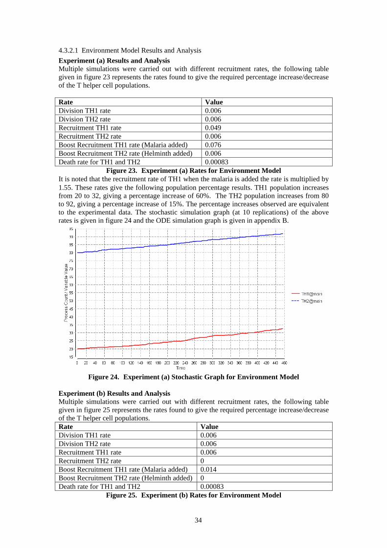
34

4.3.2.1 Environment Model Results and Analysis Experiment (a) Results and Analysis Multiple simulations were carried out with different recruitment rates, the following table given in figure 23 represents the rates found to give the required percentage increase/decrease of the T helper cell populations. Rate Value Division TH1 rate 0.006 Division TH2 rate 0.006 Recruitment TH1 rate 0.049 Recruitment TH2 rate 0.006 Boost Recruitment TH1 rate (Malaria added) 0.076 Boost Recruitment TH2 rate (Helminth added) 0.006 Death rate for TH1 and TH2 0.00083

Figure 23. Experiment (a) Rates for Environment Model It is noted that the recruitment rate of TH1 when the malaria is added the rate is multiplied by 1.55. These rates give the following population percentage results. TH1 population increases from 20 to 32, giving a percentage increase of 60%. The TH2 population increases from 80 to 92, giving a percentage increase of 15%. The percentage increases observed are equivalent to the experimental data. The stochastic simulation graph (at 10 replications) of the above rates is given in figure 24 and the ODE simulation graph is given in appendix B.

Figure 24. Experiment (a) Stochastic Graph for Environment Model

Experiment (b) Results and Analysis Multiple simulations were carried out with different recruitment rates, the following table given in figure 25 represents the rates found to give the required percentage increase/decrease of the T helper cell populations. Rate Value Division TH1 rate 0.006 Division TH2 rate 0.006 Recruitment TH1 rate 0.006 Recruitment TH2 rate 0 Boost Recruitment TH1 rate (Malaria added) 0.014 Boost Recruitment TH2 rate (Helminth added) 0 Death rate for TH1 and TH2 0.00083

Figure 25. Experiment (b) Rates for Environment Model

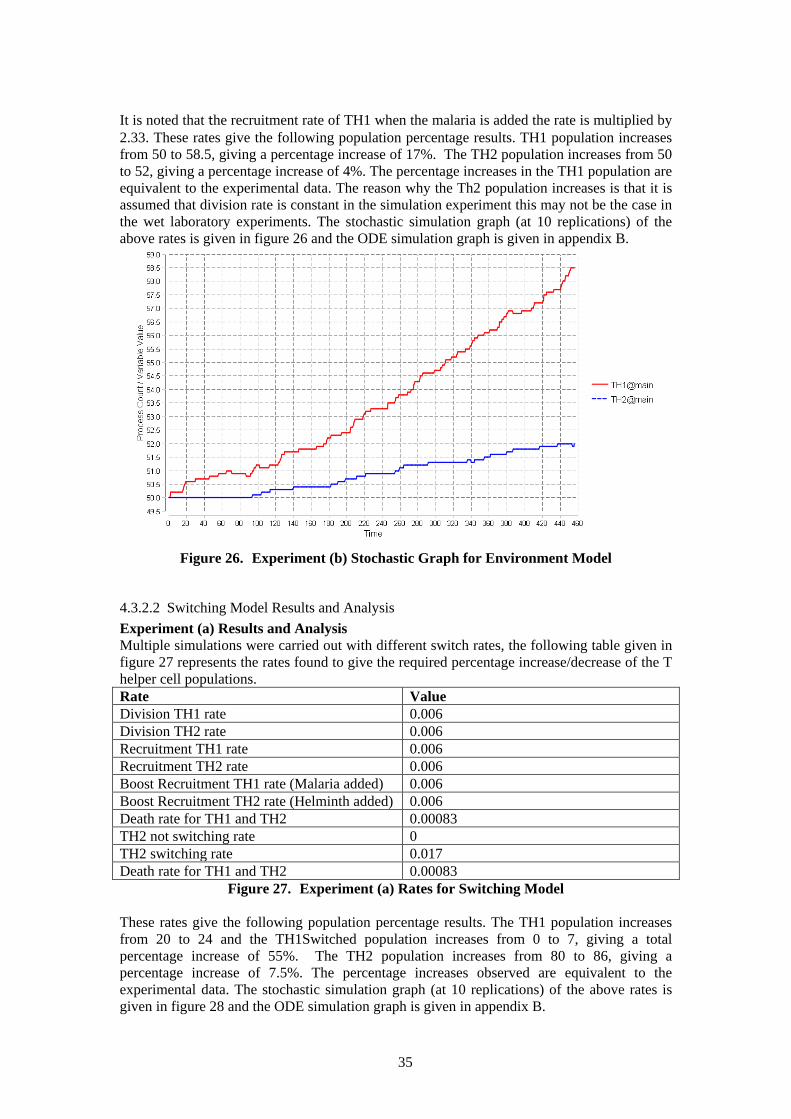
35

It is noted that the recruitment rate of TH1 when the malaria is added the rate is multiplied by 2.33. These rates give the following population percentage results. TH1 population increases from 50 to 58.5, giving a percentage increase of 17%. The TH2 population increases from 50 to 52, giving a percentage increase of 4%. The percentage increases in the TH1 population are equivalent to the experimental data. The reason why the Th2 population increases is that it is assumed that division rate is constant in the simulation experiment this may not be the case in the wet laboratory experiments. The stochastic simulation graph (at 10 replications) of the above rates is given in figure 26 and the ODE simulation graph is given in appendix B.

Figure 26. Experiment (b) Stochastic Graph for Environment Model

4.3.2.2 Switching Model Results and Analysis Experiment (a) Results and Analysis Multiple simulations were carried out with different switch rates, the following table given in figure 27 represents the rates found to give the required percentage increase/decrease of the T helper cell populations. Rate Value Division TH1 rate 0.006 Division TH2 rate 0.006 Recruitment TH1 rate 0.006 Recruitment TH2 rate 0.006 Boost Recruitment TH1 rate (Malaria added) 0.006 Boost Recruitment TH2 rate (Helminth added) 0.006 Death rate for TH1 and TH2 0.00083 TH2 not switching rate 0 TH2 switching rate 0.017 Death rate for TH1 and TH2 0.00083

Figure 27. Experiment (a) Rates for Switching Model These rates give the following population percentage results. The TH1 population increases from 20 to 24 and the TH1Switched population increases from 0 to 7, giving a total percentage increase of 55%. The TH2 population increases from 80 to 86, giving a percentage increase of 7.5%. The percentage increases observed are equivalent to the experimental data. The stochastic simulation graph (at 10 replications) of the above rates is given in figure 28 and the ODE simulation graph is given in appendix B.

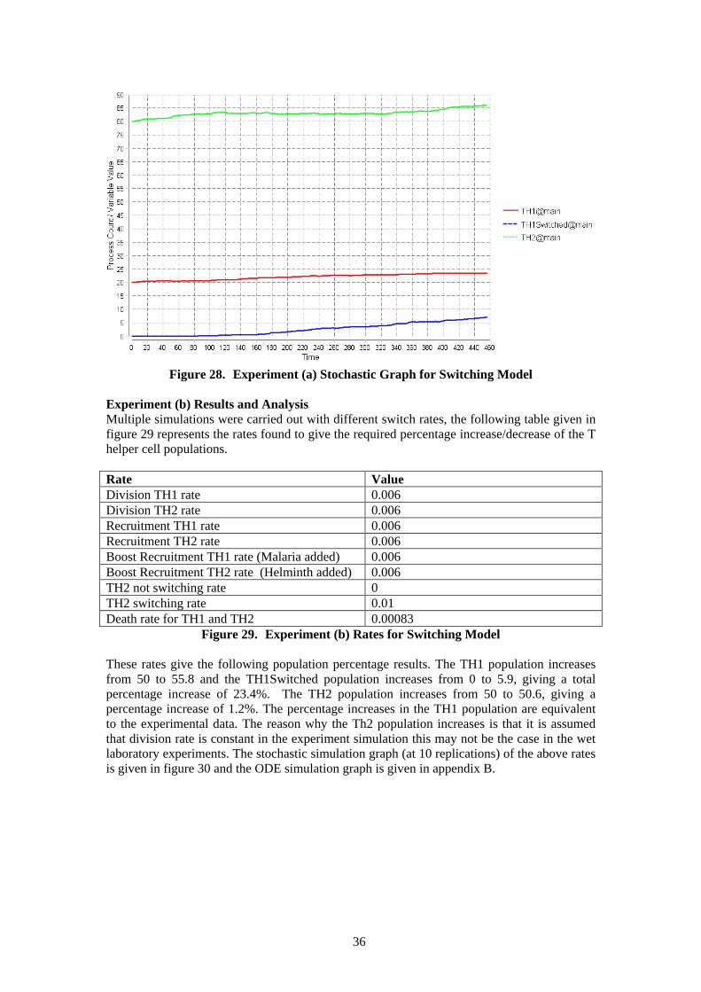
36

Figure 28. Experiment (a) Stochastic Graph for Switching Model

Experiment (b) Results and Analysis Multiple simulations were carried out with different switch rates, the following table given in figure 29 represents the rates found to give the required percentage increase/decrease of the T helper cell populations. Rate Value Division TH1 rate 0.006 Division TH2 rate 0.006 Recruitment TH1 rate 0.006 Recruitment TH2 rate 0.006 Boost Recruitment TH1 rate (Malaria added) 0.006 Boost Recruitment TH2 rate (Helminth added) 0.006 TH2 not switching rate 0 TH2 switching rate 0.01 Death rate for TH1 and TH2 0.00083

Figure 29. Experiment (b) Rates for Switching Model These rates give the following population percentage results. The TH1 population increases from 50 to 55.8 and the TH1Switched population increases from 0 to 5.9, giving a total percentage increase of 23.4%. The TH2 population increases from 50 to 50.6, giving a percentage increase of 1.2%. The percentage increases in the TH1 population are equivalent to the experimental data. The reason why the Th2 population increases is that it is assumed that division rate is constant in the experiment simulation this may not be the case in the wet laboratory experiments. The stochastic simulation graph (at 10 replications) of the above rates is given in figure 30 and the ODE simulation graph is given in appendix B.

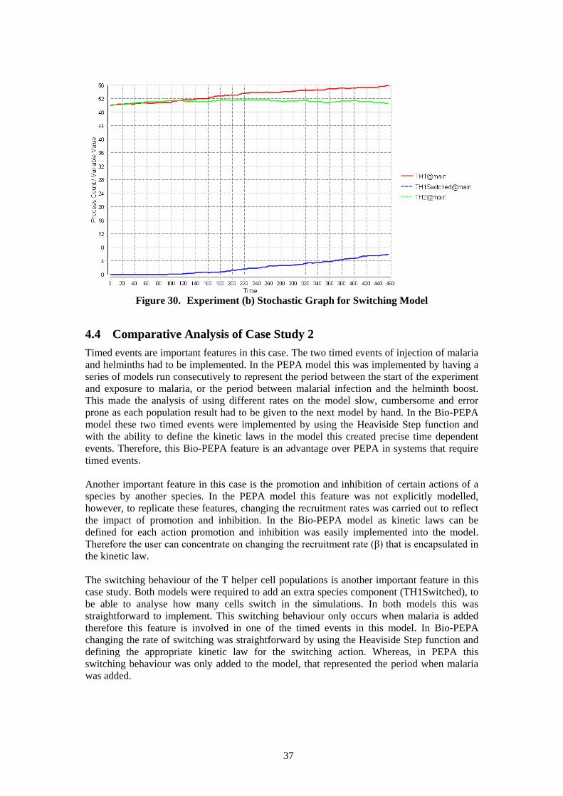
37

Figure 30. Experiment (b) Stochastic Graph for Switching Model

4.4 Comparative Analysis of Case Study 2 Timed events are important features in this case. The two timed events of injection of malaria and helminths had to be implemented. In the PEPA model this was implemented by having a series of models run consecutively to represent the period between the start of the experiment and exposure to malaria, or the period between malarial infection and the helminth boost. This made the analysis of using different rates on the model slow, cumbersome and error prone as each population result had to be given to the next model by hand. In the Bio-PEPA model these two timed events were implemented by using the Heaviside Step function and with the ability to define the kinetic laws in the model this created precise time dependent events. Therefore, this Bio-PEPA feature is an advantage over PEPA in systems that require timed events. Another important feature in this case is the promotion and inhibition of certain actions of a species by another species. In the PEPA model this feature was not explicitly modelled, however, to replicate these features, changing the recruitment rates was carried out to reflect the impact of promotion and inhibition. In the Bio-PEPA model as kinetic laws can be defined for each action promotion and inhibition was easily implemented into the model. Therefore the user can concentrate on changing the recruitment rate (β) that is encapsulated in the kinetic law. The switching behaviour of the T helper cell populations is another important feature in this case study. Both models were required to add an extra species component (TH1Switched), to be able to analyse how many cells switch in the simulations. In both models this was straightforward to implement. This switching behaviour only occurs when malaria is added therefore this feature is involved in one of the timed events in this model. In Bio-PEPA changing the rate of switching was straightforward by using the Heaviside Step function and defining the appropriate kinetic law for the switching action. Whereas, in PEPA this switching behaviour was only added to the model, that represented the period when malaria was added.

38

The death of T helper cells is another feature in this case study. In the PEPA model death was not implemented as it was thought that this would make the model more complex and may not have had much impact as the rate was small. In the Bio-PEPA model death was implemented by adding an extra action and defining kinetic laws for each species. This feature is easy utilised in Bio-PEPA. In this case study the original data was compared with the outputs of models of both languages. Calculations for the percentage increase/decrease over time were carried out on the original data to compare the results with both models. Both languages could produce stochastic and ODE simulation results to compare with the original data. In the case of PEPA the simulation results were split up as a series of models and therefore there was no visual representation of the whole simulation. The disadvantage of this is not being able to see any patterns or unusual occurrences. In Bio-PEPA one simulation graph represents the entire experiment; therefore this gives a better visualisation of the overall simulation. Location is not a main feature for this case study; although, if the models were to be extended to reflect recruitment based on proximity this would become a feature. Bio-PEPA has inbuilt location elements language features and therefore these elements can be used in this case, however, it would be important to consider what actions can occur in the different locations and the movement of the species from one location to another. This would involve creating more actions and their kinetic rates. PEPA has no spatial or location elements. When modelling location the language syntax restricts the user therefore, this part of the system may become inelegant and may not represent the true nature of the system. To conclude, PEPA is useful to begin with to obtain an understanding of the individual elements of the system. To be able to carry out analysis of the overall system it is more straightforward to implement models in Bio-PEPA because of its ability to handle timed events and promotion and inhibition of actions caused by species. Although both models are equally straightforward in incorporating the switching behaviour of Th populations, Bio-PEPA visualisation analysis of the whole experiment simulation is much simpler. In choosing to model, if timed events and promotion and inhibition are important elements of the system the language recommended to use is Bio-PEPA.

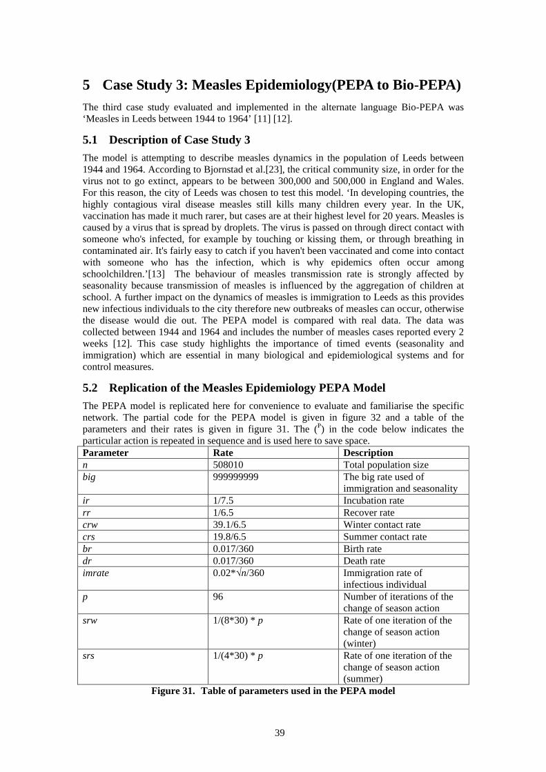
39

5 Case Study 3: Measles Epidemiology(PEPA to Bio-PEPA) The third case study evaluated and implemented in the alternate language Bio-PEPA was ‘Measles in Leeds between 1944 to 1964’ [11] [12].

5.1 Description of Case Study 3 The model is attempting to describe measles dynamics in the population of Leeds between 1944 and 1964. According to Bjornstad et al.[23], the critical community size, in order for the virus not to go extinct, appears to be between 300,000 and 500,000 in England and Wales. For this reason, the city of Leeds was chosen to test this model. ‘In developing countries, the highly contagious viral disease measles still kills many children every year. In the UK, vaccination has made it much rarer, but cases are at their highest level for 20 years. Measles is caused by a virus that is spread by droplets. The virus is passed on through direct contact with someone who's infected, for example by touching or kissing them, or through breathing in contaminated air. It's fairly easy to catch if you haven't been vaccinated and come into contact with someone who has the infection, which is why epidemics often occur among schoolchildren.’[13] The behaviour of measles transmission rate is strongly affected by seasonality because transmission of measles is influenced by the aggregation of children at school. A further impact on the dynamics of measles is immigration to Leeds as this provides new infectious individuals to the city therefore new outbreaks of measles can occur, otherwise the disease would die out. The PEPA model is compared with real data. The data was collected between 1944 and 1964 and includes the number of measles cases reported every 2 weeks [12]. This case study highlights the importance of timed events (seasonality and immigration) which are essential in many biological and epidemiological systems and for control measures.

5.2 Replication of the Measles Epidemiology PEPA Model The PEPA model is replicated here for convenience to evaluate and familiarise the specific network. The partial code for the PEPA model is given in figure 32 and a table of the parameters and their rates is given in figure 31. The (P) in the code below indicates the particular action is repeated in sequence and is used here to save space. Parameter Rate Description n 508010 Total population size big 999999999 The big rate used of

immigration and seasonality ir 1/7.5 Incubation rate rr 1/6.5 Recover rate crw 39.1/6.5 Winter contact rate crs 19.8/6.5 Summer contact rate br 0.017/360 Birth rate dr 0.017/360 Death rate imrate 0.02*√n/360 Immigration rate of

infectious individual p 96 Number of iterations of the

change of season action srw 1/(8*30) * p Rate of one iteration of the

change of season action (winter)

srs 1/(4*30) * p Rate of one iteration of the change of season action (summer)

Figure 31. Table of parameters used in the PEPA model

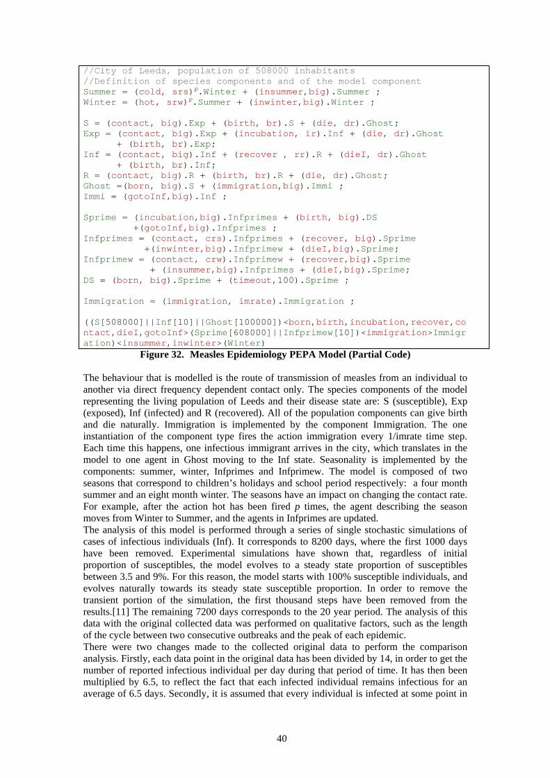
40

//City of Leeds, population of 508000 inhabitants //Definition of species components and of the model component Summer = (cold, srs)p.Winter + (insummer,big).Summer ; Winter = (hot, srw)p.Summer + (inwinter,big).Winter ; S = (contact, big).Exp + (birth, br).S + (die, dr).Ghost; Exp = (contact, big).Exp + (incubation, ir).Inf + (die, dr).Ghost + (birth, br).Exp; Inf = (contact, big).Inf + (recover , rr).R + (dieI, dr).Ghost + (birth, br).Inf; R = (contact, big).R + (birth, br).R + (die, dr).Ghost; Ghost =(born, big).S + (immigration,big).Immi ; Immi = (gotoInf,big).Inf ; Sprime = (incubation,big).Infprimes + (birth, big).DS +(gotoInf,big).Infprimes ; Infprimes = (contact, crs).Infprimes + (recover, big).Sprime +(inwinter,big).Infprimew + (dieI,big).Sprime; Infprimew = (contact, crw).Infprimew + (recover,big).Sprime + (insummer,big).Infprimes + (dieI,big).Sprime; DS = (born, big).Sprime + (timeout,100).Sprime ; Immigration = (immigration, imrate).Immigration ; ((S[508000]||Inf[10]||Ghost[100000])<born,birth,incubation,recover,contact,dieI,gotoInf>(Sprime[608000]||Infprimew[10])<immigration>Immigration)<insummer,inwinter>(Winter)

Figure 32. Measles Epidemiology PEPA Model (Partial Code) The behaviour that is modelled is the route of transmission of measles from an individual to another via direct frequency dependent contact only. The species components of the model representing the living population of Leeds and their disease state are: S (susceptible), Exp (exposed), Inf (infected) and R (recovered). All of the population components can give birth and die naturally. Immigration is implemented by the component Immigration. The one instantiation of the component type fires the action immigration every 1/imrate time step. Each time this happens, one infectious immigrant arrives in the city, which translates in the model to one agent in Ghost moving to the Inf state. Seasonality is implemented by the components: summer, winter, Infprimes and Infprimew. The model is composed of two seasons that correspond to children’s holidays and school period respectively: a four month summer and an eight month winter. The seasons have an impact on changing the contact rate. For example, after the action hot has been fired p times, the agent describing the season moves from Winter to Summer, and the agents in Infprimes are updated. The analysis of this model is performed through a series of single stochastic simulations of cases of infectious individuals (Inf). It corresponds to 8200 days, where the first 1000 days have been removed. Experimental simulations have shown that, regardless of initial proportion of susceptibles, the model evolves to a steady state proportion of susceptibles between 3.5 and 9%. For this reason, the model starts with 100% susceptible individuals, and evolves naturally towards its steady state susceptible proportion. In order to remove the transient portion of the simulation, the first thousand steps have been removed from the results.[11] The remaining 7200 days corresponds to the 20 year period. The analysis of this data with the original collected data was performed on qualitative factors, such as the length of the cycle between two consecutive outbreaks and the peak of each epidemic. There were two changes made to the collected original data to perform the comparison analysis. Firstly, each data point in the original data has been divided by 14, in order to get the number of reported infectious individual per day during that period of time. It has then been multiplied by 6.5, to reflect the fact that each infected individual remains infectious for an average of 6.5 days. Secondly, it is assumed that every individual is infected at some point in

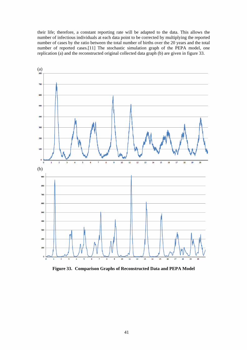
41

their life; therefore, a constant reporting rate will be adapted to the data. This allows the number of infectious individuals at each data point to be corrected by multiplying the reported number of cases by the ratio between the total number of births over the 20 years and the total number of reported cases.[11] The stochastic simulation graph of the PEPA model, one replication (a) and the reconstructed original collected data graph (b) are given in figure 33. (a)

(b)

Figure 33. Comparison Graphs of Reconstructed Data and PEPA Model

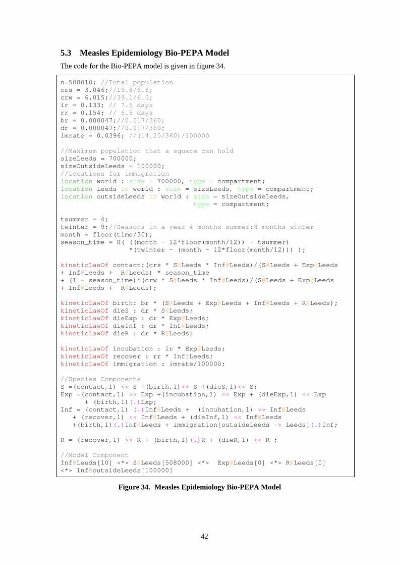
42

5.3 Measles Epidemiology Bio-PEPA Model The code for the Bio-PEPA model is given in figure 34.

n=508010; //Total population crs = 3.046;//19.8/6.5; crw = 6.015;//39.1/6.5; ir = 0.133; // 7.5 days rr = 0.154; // 6.5 days br = 0.000047;//0.017/360; dr = 0.000047;//0.017/360; imrate = 0.0396; //(14.25/360)/100000 //Maximum population that a square can hold sizeLeeds = 700000; sizeOutsideLeeds = 100000; //Locations for immigration location world : size = 700000, type = compartment; location Leeds in world : size = sizeLeeds, type = compartment; location outsideLeeds in world : size = sizeOutsideLeeds, type = compartment; tsummer = 4; twinter = 9;//Seasons in a year 4 months summer:8 months winter month = floor(time/30); season_time = H( ((month - 12*floor(month/12)) - tsummer) *(twinter - (month - 12*floor(month/12))) ); kineticLawOf contact:(crs * S@Leeds * Inf@Leeds)/(S@Leeds + Exp@Leeds + Inf@Leeds + R@Leeds) * season_time + (1 - season_time)*(crw * S@Leeds * Inf@Leeds)/(S@Leeds + Exp@Leeds + Inf@Leeds + R@Leeds); kineticLawOf birth: br * (S@Leeds + Exp@Leeds + Inf@Leeds + R@Leeds); kineticLawOf dieS : dr * S@Leeds; kineticLawOf dieExp : dr * Exp@Leeds; kineticLawOf dieInf : dr * Inf@Leeds; kineticLawOf dieR : dr * R@Leeds; kineticLawOf incubation : ir * Exp@Leeds; kineticLawOf recover : rr * Inf@Leeds; kineticLawOf immigration : imrate/100000; //Species Components S =(contact,1) << S +(birth,1)>> S +(dieS,1)<< S; Exp =(contact,1) >> Exp +(incubation,1) << Exp + (dieExp,1) << Exp + (birth,1)(.)Exp; Inf = (contact,1) (.)Inf@Leeds + (incubation,1) >> Inf@Leeds + (recover,1) << Inf@Leeds + (dieInf,1) << Inf@Leeds +(birth,1)(.)Inf@Leeds + immigration[outsideLeeds -> Leeds](.)Inf; R = (recover,1) >> R + (birth,1)(.)R + (dieR,1) << R ; //Model Component Inf@Leeds[10] <*> S@Leeds[508000] <*> Exp@Leeds[0] <*> R@Leeds[0] <*> Inf@outsideLeeds[100000]

Figure 34. Measles Epidemiology Bio-PEPA Model

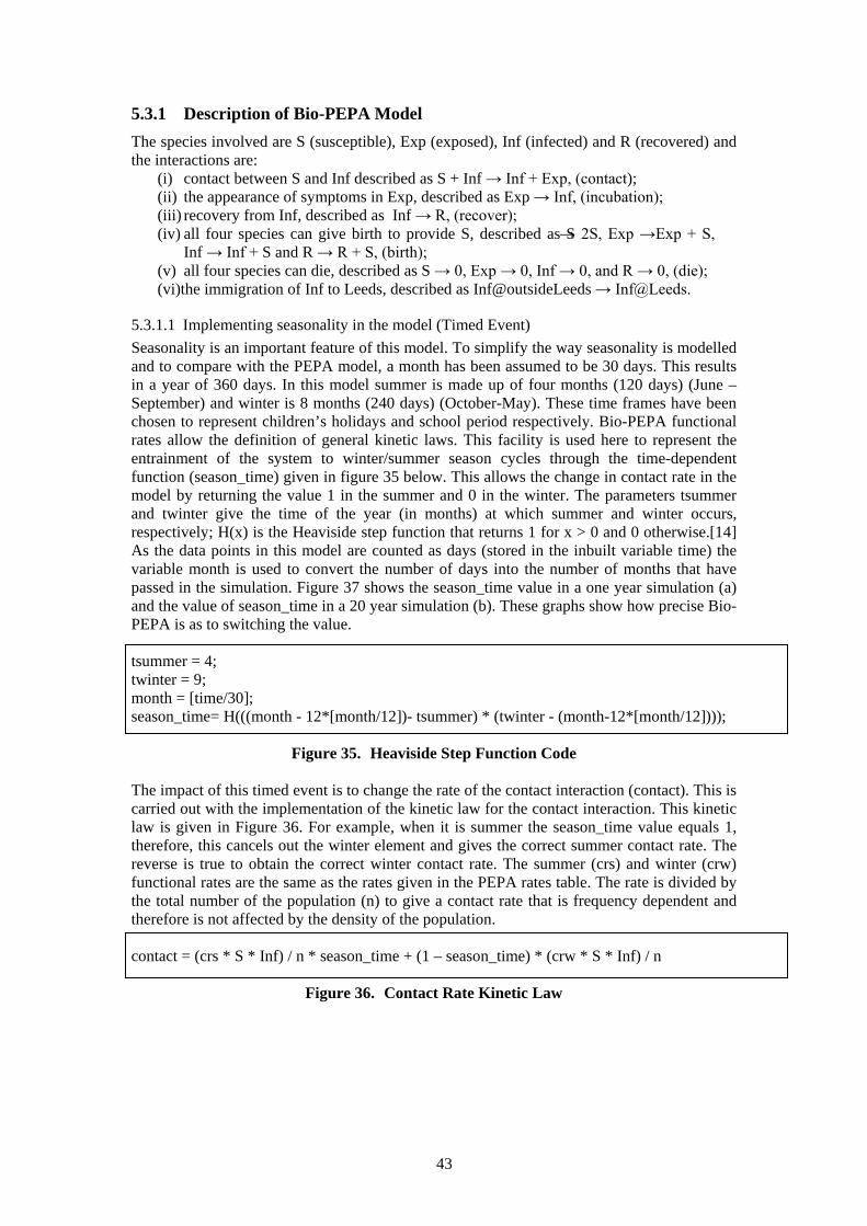
43

5.3.1 Description of Bio-PEPA Model The species involved are S (susceptible), Exp (exposed), Inf (infected) and R (recovered) and the interactions are:

(i) contact between S and Inf described as S + Inf → Inf + Exp, (contact); (ii) the appearance of symptoms in Exp, described as Exp → Inf, (incubation); (iii) recovery from Inf, described as Inf → R, (recover); (iv) all four species can give birth to provide S, described as S → 2S, Exp →Exp + S,

Inf → Inf + S and R → R + S, (birth); (v) all four species can die, described as S → 0, Exp → 0, Inf → 0, and R → 0, (die); (vi)the immigration of Inf to Leeds, described as Inf@outsideLeeds → Inf@Leeds.

5.3.1.1 Implementing seasonality in the model (Timed Event) Seasonality is an important feature of this model. To simplify the way seasonality is modelled and to compare with the PEPA model, a month has been assumed to be 30 days. This results in a year of 360 days. In this model summer is made up of four months (120 days) (June –September) and winter is 8 months (240 days) (October-May). These time frames have been chosen to represent children’s holidays and school period respectively. Bio-PEPA functional rates allow the definition of general kinetic laws. This facility is used here to represent the entrainment of the system to winter/summer season cycles through the time-dependent function (season_time) given in figure 35 below. This allows the change in contact rate in the model by returning the value 1 in the summer and 0 in the winter. The parameters tsummer and twinter give the time of the year (in months) at which summer and winter occurs, respectively; H(x) is the Heaviside step function that returns 1 for x > 0 and 0 otherwise.[14] As the data points in this model are counted as days (stored in the inbuilt variable time) the variable month is used to convert the number of days into the number of months that have passed in the simulation. Figure 37 shows the season_time value in a one year simulation (a) and the value of season_time in a 20 year simulation (b). These graphs show how precise Bio-PEPA is as to switching the value. tsummer = 4; twinter = 9; month = [time/30]; season_time= H(((month - 12*[month/12])- tsummer) * (twinter - (month-12*[month/12])));

Figure 35. Heaviside Step Function Code The impact of this timed event is to change the rate of the contact interaction (contact). This is carried out with the implementation of the kinetic law for the contact interaction. This kinetic law is given in Figure 36. For example, when it is summer the season_time value equals 1, therefore, this cancels out the winter element and gives the correct summer contact rate. The reverse is true to obtain the correct winter contact rate. The summer (crs) and winter (crw) functional rates are the same as the rates given in the PEPA rates table. The rate is divided by the total number of the population (n) to give a contact rate that is frequency dependent and therefore is not affected by the density of the population. contact = (crs * S * Inf) / n * season_time + (1 – season_time) * (crw * S * Inf) / n

Figure 36. Contact Rate Kinetic Law

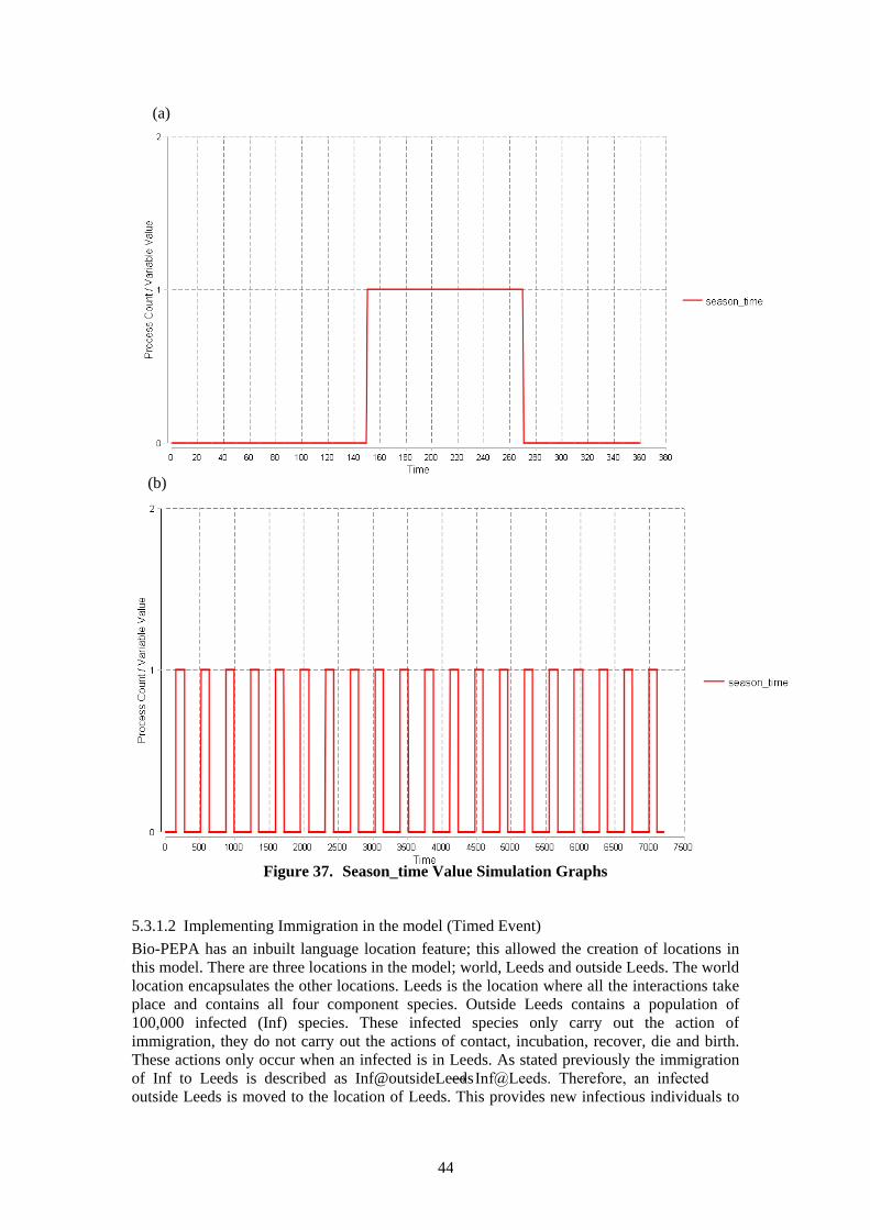
44

(a)

(b)

Figure 37. Season_time Value Simulation Graphs

5.3.1.2 Implementing Immigration in the model (Timed Event) Bio-PEPA has an inbuilt language location feature; this allowed the creation of locations in this model. There are three locations in the model; world, Leeds and outside Leeds. The world location encapsulates the other locations. Leeds is the location where all the interactions take place and contains all four component species. Outside Leeds contains a population of 100,000 infected (Inf) species. These infected species only carry out the action of immigration, they do not carry out the actions of contact, incubation, recover, die and birth. These actions only occur when an infected is in Leeds. As stated previously the immigration of Inf to Leeds is described as Inf@outsideLeeds → Inf@Leeds. Therefore, an infected outside Leeds is moved to the location of Leeds. This provides new infectious individuals to

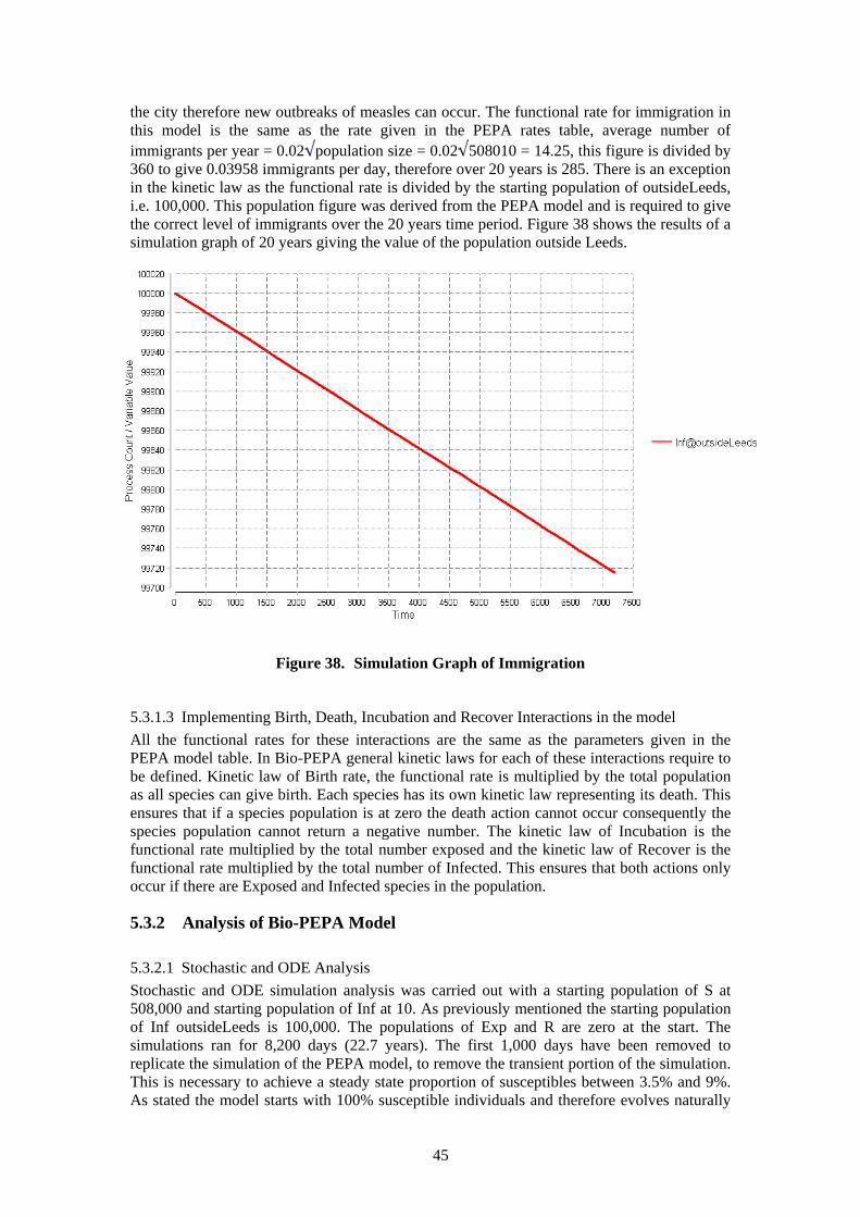
45

the city therefore new outbreaks of measles can occur. The functional rate for immigration in this model is the same as the rate given in the PEPA rates table, average number of immigrants per year = 0.02 population size = 0.02 508010 = 14.25, this figure is divided by 360 to give 0.03958 immigrants per day, therefore over 20 years is 285. There is an exception in the kinetic law as the functional rate is divided by the starting population of outsideLeeds, i.e. 100,000. This population figure was derived from the PEPA model and is required to give the correct level of immigrants over the 20 years time period. Figure 38 shows the results of a simulation graph of 20 years giving the value of the population outside Leeds.

Figure 38. Simulation Graph of Immigration

5.3.1.3 Implementing Birth, Death, Incubation and Recover Interactions in the model All the functional rates for these interactions are the same as the parameters given in the PEPA model table. In Bio-PEPA general kinetic laws for each of these interactions require to be defined. Kinetic law of Birth rate, the functional rate is multiplied by the total population as all species can give birth. Each species has its own kinetic law representing its death. This ensures that if a species population is at zero the death action cannot occur consequently the species population cannot return a negative number. The kinetic law of Incubation is the functional rate multiplied by the total number exposed and the kinetic law of Recover is the functional rate multiplied by the total number of Infected. This ensures that both actions only occur if there are Exposed and Infected species in the population.

5.3.2 Analysis of Bio-PEPA Model

5.3.2.1 Stochastic and ODE Analysis Stochastic and ODE simulation analysis was carried out with a starting population of S at 508,000 and starting population of Inf at 10. As previously mentioned the starting population of Inf outsideLeeds is 100,000. The populations of Exp and R are zero at the start. The simulations ran for 8,200 days (22.7 years). The first 1,000 days have been removed to replicate the simulation of the PEPA model, to remove the transient portion of the simulation. This is necessary to achieve a steady state proportion of susceptibles between 3.5% and 9%. As stated the model starts with 100% susceptible individuals and therefore evolves naturally

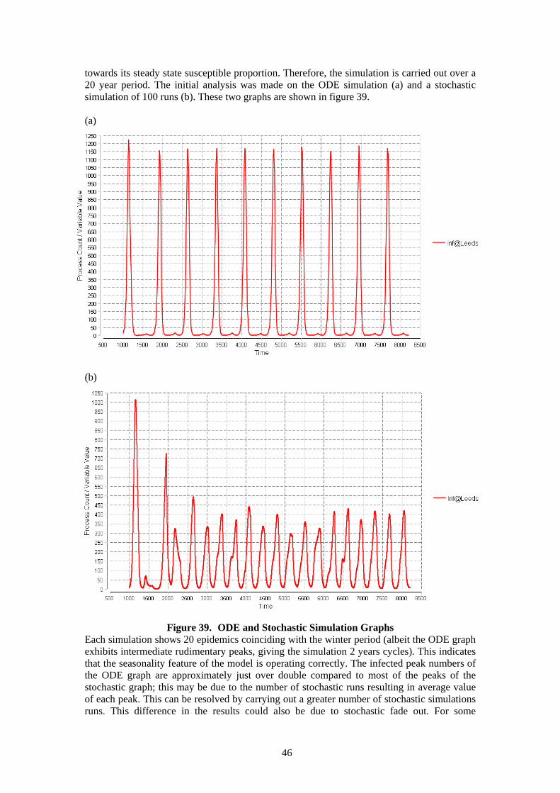
46

towards its steady state susceptible proportion. Therefore, the simulation is carried out over a 20 year period. The initial analysis was made on the ODE simulation (a) and a stochastic simulation of 100 runs (b). These two graphs are shown in figure 39. (a)

(b)

Figure 39. ODE and Stochastic Simulation Graphs

Each simulation shows 20 epidemics coinciding with the winter period (albeit the ODE graph exhibits intermediate rudimentary peaks, giving the simulation 2 years cycles). This indicates that the seasonality feature of the model is operating correctly. The infected peak numbers of the ODE graph are approximately just over double compared to most of the peaks of the stochastic graph; this may be due to the number of stochastic runs resulting in average value of each peak. This can be resolved by carrying out a greater number of stochastic simulations runs. This difference in the results could also be due to stochastic fade out. For some

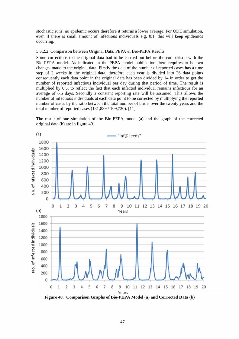
47

stochastic runs, no epidemic occurs therefore it returns a lower average. For ODE simulation, even if there is small amount of infectious individuals e.g. 0.1, this will keep epidemics occurring.

5.3.2.2 Comparison between Original Data, PEPA & Bio-PEPA Results Some corrections to the original data had to be carried out before the comparison with the Bio-PEPA model. As indicated in the PEPA model publication there requires to be two changes made to the original data. Firstly the data of the number of reported cases has a time step of 2 weeks in the original data, therefore each year is divided into 26 data points consequently each data point in the original data has been divided by 14 in order to get the number of reported infectious individual per day during that period of time. The result is multiplied by 6.5, to reflect the fact that each infected individual remains infectious for an average of 6.5 days. Secondly a constant reporting rate will be assumed. This allows the number of infectious individuals at each data point to be corrected by multiplying the reported number of cases by the ratio between the total number of births over the twenty years and the total number of reported cases (181,839 / 109,730). [11] The result of one simulation of the Bio-PEPA model (a) and the graph of the corrected original data (b) are in figure 40. (a)

(b)

Figure 40. Comparison Graphs of Bio-PEPA Model (a) and Corrected Data (b)

48

The two graphs show similar behaviour, both have regular cycles of measles outbreaks. Most of the cycles are similar in length of cycles lasting approximately 2 years. Where the cycles differ in the Bio-PEPA simulation is between years 1950 and 1952 (6 to 8 on graph), between 1952 and 1954 (8 to 10 on graph) and between 1960 and 1962 (16 to 18 on graph) as outbreaks of measles occur each year specified, whereas in the rest of the time period there is one outbreak per every 2 years. It is noted in corrected original data graph that in between 1948 to 1950 (4 to 6 on graph), between 1950 to 1952 (6 to 8 on graph) and between 1952 to 1954 (8 to 10 on graph) outbreaks occur each year although the peaks in year 4,6 and 8 are in a lower range than the simulation peaks. The corrected original data experiences 13 outbreaks: this includes the lower peaks above 200 and the simulation also experiences 13 outbreaks of measles. The values of the peaks of infection fluctuate in both graphs: for the corrected original data graph the minimum value is 230 and the maximum value is 1600. For the Bio-PEPA simulation the minimum value is 400 and the maximum is 1800. This difference of values is confirmed by the average number of individuals at the peak of each outbreak which is 713 in the corrected original data and 950 in the Bio-PEPA simulation.

5.4 Comparative Analysis of Case Study 3 Timed events are important features in this case study. In particular seasonality had to be implemented in the languages. In PEPA it is not possible to specify precisely when an action should be fired as the rate at which that action happens follows a cumulative distribution function which only ensures that an average action will be fired after 1/rate time steps. To implement the seasonality into the PEPA model a single component agent was created to fire at regular intervals. This agent had the action that would be fired split into several steps to lower the variability on the actual moment at which the action takes place. [11] This means the season rate change does not flip at a precise time. In contrast the Bio-PEPA language does have an inbuilt events feature; however, this is not built in the plug-in. Using the Heaviside Step function, the use of the inbuilt “time” variable and with the ability to define the kinetic laws in the model this created precise time dependent events. The season rate change flips at a precise time. Therefore, this Bio-PEPA feature is an advantage over PEPA in systems that require timed events. Location is another important feature in this case study. The immigration of infected individuals had to be built into the models. Immigration in the PEPA model has been implemented using the same method as seasonality, by using a single component agent, although the action of this component is not spilt. As there is no spatial or location elements language features in PEPA a component agent was implemented in this case called Ghost to become an infected individual when the immigration action is fired. When modelling location in PEPA the language syntax restricts the user and therefore, this part of the system appears inelegant and does not represent the true descriptive nature of the system. In comparison to PEPA, Bio-PEPA has inbuilt location elements language features which are intuitive to the user. Therefore, creation of the different locations of this system and the creation of the immigration action using the direction action feature of Bio-PEPA is uncomplicated; although, it is important to consider what actions the species components perform in the locations. For example, when the infectious individuals are outside Leeds they do not give birth, die or recover: only infected individuals in Leeds should fulfil these actions. Bio-PEPA provides a more elegant and representative description of locations required in a system. Birth and death is another feature in this case study. In the PEPA model birth and death was implemented by using the agent Ghost population. PEPA has no inbuilt features to increase or decrease a population based on an action, another component agent must be used to implement this feature. In the Bio-PEPA model birth and death was implemented by adding actions with operations (product >> and reactant <<) respectively to define the increase and decrease of the populations of the species.

49

In this case study the original data was compared with the models of both languages. This original data had to be corrected for analysis comparison with the simulation results. Both languages could produce stochastic simulation results that were available to compare with the data. ODE results of the PEPA model were not reliable due to the operation of the events in the PEPA model. In contrast, ODE results of the Bio-PEPA model are available and aid in the analysis of this model. In terms of achieving stochastic results the preparation of the start time, end time and replication numbers was straightforward. A disadvantage observed in Bio-PEPA is the manual creation of kinetic laws for each action. For example, the immigration kinetic law where the functional rate is divided by the total starting population of outsideLeeds may not be obvious to the user initially. The user has to be particularly careful to create the correct kinetic laws to create the accurate system behaviour. When introducing a kinetic law to the system it is important to test the model at each stage by analysing simulations to ensure the kinetic laws describe the system correctly. An advantage in PEPA is that the kinetic laws are automatically generated by PEPA, therefore the user can concentrate on building the model to simulate the correct behaviour of the specific system. An advantage observed in Bio-PEPA of having manual kinetic laws is that the user can immediately introduce the influence specific populations have with the rates of specific actions. For example, the birth rate is influenced by the total population of Leeds. To conclude, in achieving an overall and descriptive view of this system the straightforward implementation of timed events and inbuilt locations in Bio-PEPA is successful compared to PEPA. In choosing to model, if timed events and locations are important elements of the system the language recommended to use is Bio-PEPA; however, the kinetic laws require to be accurate to achieve the exact system.

50

6 Conclusion

6.1 Comparison Analysis Evaluation The case studies have been modelled equally in PEPA and Bio-PEPA. This means that both languages are capable of expressing these biological systems; however, PEPA and Bio-PEPA languages express the biological systems differently. The recommendations are based on how simply or problematical both languages express the biological systems. To evaluate which language is more appropriate to model a specific biological system, specific prerequisites require to be analysed concerning the system. Initially the basic fundamentals of the system must be established; for example, the number and type of species (molecules, cells or life forms) that is within the system. These preliminary questions impact on the necessary abstraction view of the system that will be implemented. Secondly, the characteristics that the system encompasses and their importance need to be analysed. For example, are spatial elements crucial to the behaviour of the system? Thirdly, the analysis techniques that can be used on models of each language, for example, how these techniques can be used to compare the model to biological data of the system. After these observations have been concluded a recommendation can be given. The following sections describe how both languages view a biological system and what features of a biological system they can incorporate and analysis techniques that can be applied.

6.1.1 Implementing a View of the System In PEPA there are two known approaches to implement the view of a biological system. The two views of PEPA have been shown to be equivalent.[21] These approaches are described as follows:

a) Reagent-centric view; the PEPA sequential components represent various concentration levels of the species. This is a low level view of the biological system, describing each reagent and their interactions.

b) Pathway-centric view; describes sub-pathways of the system (which the reagents are in). This is a higher level view of the biological system, describing each sub-pathway in what actions and interactions occurs within it.[5]

Both these views have advantages and disadvantages to the modeller. The reagent-centric model has explicit concentrations (fine view) whilst in the pathway-centric model the concentrations are captured only implicitly (coarse view) via the possible activities of each sub-pathway. The pathway-centric model is less directly expressive; however, it captures the same behaviour as the other approach.[21] The advantage of PEPA having these two equivalent approaches is that two representations of a large biological model can be used interchangeably. Calder et al suggest a model could be implemented with the key pathway being modelled using the reagent-centric approach whilst the peripheral pathways of the system could be modelled using the pathway-centric approach.[21] This allows the modeller to concentrate on the main parts of the system and abstract away from the marginal parts of the system. Therefore PEPA may be the appropriate language to use with large biological systems such as signalling pathways.[5] Bio-PEPA is a modification of PEPA which makes it possible to represent explicitly features of biochemical models, specifically the stoichiometry and the role of the species in a given reaction. Also kinetic laws can be implemented to represent each action’s functional rate. Bio-PEPA is equipped with an operational semantics and a stochastic labelled transition system based on discrete levels of concentration. Therefore, Bio-PEPA models are implemented in the reagent-centric view.[5] The advantage of this is that Bio-PEPA models will have an explicitly descriptive view of the biological system.

51

6.1.2 Implementing Features of the System Every biological system has features encapsulated that play an important role in the overall network. It is therefore important to identify which process algebra language incorporates the necessary features in the most appropriate way. There are a wide range of diverse features across biological systems. In this project the focus was placed on specific features these are described as follows; space, timed events, birth and death, inhibition and promotion and phenotypic switching. The case studies were chosen to highlight these features. The crowd dynamic case study discussed in section 3 was chosen as it has spatial elements and this emphasizes how the two languages handle the implementation of locations in a model. The immunological case study referred in section 4 was chosen as it incorporates biological inhibition and promotion, death and timed events. The measles epidemiology case study referred in section 5 was chosen as it also had spatial elements, birth and death and the introduction of timed events to the model. This was to further develop the understanding and recommendations for the comparison. The following recommendations are given for these features as to which language defines and incorporates the given feature most appropriately.

6.1.2.1 Space (Location) If the system has to have knowledge of proximity, spatial locations are important. For example, this could refer to movement of species (people, cells, molecules) from one location to another to actions only taking place in specific locations. Bio-PEPA has inbuilt language features which allows the user to create spatial elements easily in the model. It also has inbuilt operations which define movement actions of species from these locations. This allows the user to concentrate on the specific kinetic laws of the movement of species from the locations and what actions occur in these locations. These features allow the user to have a more abstract view of the system because it focuses on the locations and the populations of species in these locations. One disadvantage is that the emphasis may be taken away from individual behaviour observations and therefore the modeller may not achieve a full understanding of this individual behaviour. PEPA does not have inbuilt features for spatial elements of a system. The modeller has to implement this feature from the given syntax of PEPA. This leads to inelegant characteristics in the model which are not realistic and does not define the system in real terms; however, as the user has to implement these features they encapsulate the individual behaviour of species. This gives the user a less abstract model of the network and better understanding of individual behaviour.

6.1.2.2 Timed Events Timed events correspond to events that happen at fixed times, either once (introduction of an injection), or regularly (circadian clock, seasonality and immigration). These are essential in many biological and epidemiological systems and for control measures.[11] Bio-PEPA has an inbuilt events feature; however, this is not built into the plug-in; nevertheless, as Bio-PEPA gives the user the ability to define kinetic laws of each action this allows the use of the Heaviside Step Function and this creates precise time dependent events. This leads to the user implementing expressions for these events in the kinetic laws, this is relatively straightforward for one off timed events; however, the expression becomes more complex when implementing repeating timed events. One advantage of using the above technique is that it gives the ability to change specific rates while the simulation is running at specific precise times. PEPA does not have an inbuilt timed event language feature; nonetheless, there are many different ways in which the user can implement timed events. Some of these implementations however inhibit the analysis of the model e.g. derivation of ODE simulations. In PEPA it is not possible to specify precisely when an action should occur and therefore it cannot define the true nature of a timed event.

52

6.1.2.3 Birth and Death This is a basic biological feature that defines the actions of adding or decreasing a species. Bio-PEPA has prefix combinators which represent the role of a species in an action or the impact that an action has on that species. Two combinators that can define birth and death of a species are product ‘>>’ and reactant ‘<<’ respectively. A reactant will be consumed in the action (decreasing the species population). A product is produced as a result of the action (increasing the species population). This allows the user to focus on specifying the correct kinetic laws for these actions. PEPA does not have these types of combinators, therefore does not define what role the species has in each action. The user must implement actions such as death and birth by having other agent populations which synchronise on the roles of increasing and decreasing the specific population. This is shown in the PEPA model in section 5. This is inelegant and distracts from the true nature of the system.

6.1.2.4 Inhibition and Promotion This biological feature defines when species populations inhibit or activate specific actions in the system. For example, as in case study 2 in section 4 the T helper cell populations inhibit and promote each other in the recruitment of naive cells. Bio-PEPA allows the user to define kinetic laws for actions and therefore this allows the user to specify which species population promote or inhibit actions of other species. This is shown in section 2.2.2 and section 4. PEPA automatically defines kinetic laws for actions in the model. Therefore in PEPA only Mass Action (elementary) reactions can be considered. Decomposing complex reactions into elementary ones is often difficult and complex.[22] This means the addition of inhibition or promotion in the PEPA language is challenging.

6.1.2.5 Phenotypic Switching Phenotypic switching may be important in models that are at cellular level. Phenotypic switching is the switching between two cell types. In both languages a similar implementation of this feature was shown. Both languages required the addition of an extra species component to analyse how many cells switch in the simulations. Therefore it was generally straightforward to implement this feature in both languages. The only down side of implementing this feature in PEPA was if the action of switching was associated with a timed event. As mentioned above in section 6.1.2.2 PEPA cannot be precise in time dependent events and therefore this may impact on the feature of switching.

6.1.3 Applied Analysis Techniques In the three case studies the analysis techniques of stochastic and ODE simulations were investigated. As mention in section 6.1.2 in the PEPA language many of the features had to be implemented by the user and therefore made the model inelegant and complex. This has an impact on what analysis techniques that can be used on the model and what analysis can be carried out on the model (e.g. investigating different starting populations). Some analysis techniques become unsuitable, therefore inhibiting the overall analysis of the biological model and impeding the investigation of the system. In Bio-PEPA, as there are inbuilt features, there was less restriction on analysis techniques. Two of the case studies were investigated as experimental data was available to compare to the model simulation results. In both languages this original data had to have minor changes made prior to it being compared to the results. Apart from these minor changes both models of each language could be compared to the original data. Although in one case in section 4 the problem addressed above in PEPA had an impact on the visualisation of the simulation results.

53

6.2 Conclusion Recommendation Summary To conclude, a summary of the recommendations are given as follows:

a) PEPA is better on average with biological systems (i) with large complex pathways (ii) where spatial elements are not important (iii) where timed events are not essential (iv) where birth and degradation of components are not required (v) where all kinetic laws are of mass action (vi) which have phenotypic switching (vi) which have experimental biological data

b) Bio-PEPA is better on average with biological systems (i) where spatial elements are important (ii) where timed events are essential (iii) where birth and degradation of components are required (iv) where the kinetic laws are elementary and complex (v) which have phenotypic switching (vi) which have experimental biological data

6.3 Future Work There are many possible areas of future work from this project. Improvements in the models could be made by implementing more realism into them. For example, in case study 1 in section 3 activities could be added to impact of an individual’s independent choice; in case study 2 in section 4 cytokine pathways could be developed to understand the lower level of the immunological system; and in case study 3 in section 5 more locations could be added to investigate further the impact of immigration to an outbreak. More analysis techniques as mentioned in section 2.1.2 could be utilised on the models to further aid in the recommendations. Also more case studies need to be investigated to strengthen the recommendations in particular larger systems such as cell signalling pathways. Further developments to the languages or a new language could incorporate more biological system features, for example, systems that require low and high level feature integration (physiology of a life form and its interaction within an ecosystem).

54

References [1] Hillston, J. A Compositional Approach to Performance. Cambridge University Press,

1996. [2] Hillston, J. Tuning Systems: From Composition To Performance, The Computer

Journal, 48(4)386-388, May 2005. [3] Tribastone, M., Duguid, A. and Gilmore, S. The PEPA Eclipse Plug-in, Performance

Evaluation Review, 36(4):28-33, March 2009. [4] Scott, E., Mahajan, S.M., Brand-Spencer, T., Allen, J.E., Norman, R., Graham, A.L. and

Shankland, C. Modelling Immunological Systems using PEPA: a preliminary report. In Bradley, J.T., Hayden, R.A. editors, 9th Workshop on Process Algebra and Stochastically Timed Activities, pages 64-69, Department of Computing Imperial College, London, September 2010.

[5] Ciocchetta, F. and Hillston, J. Bio-PEPA: A Framework for the Modelling and Analysis of Biochemical Networks, Theoretical Computer Science 410 (33-34): 8,27-30, 2009

[6] University of Edinburgh. Bio-PEPA home page, http://homepages.inf.ed.ac.uk/jeh/Bio-PEPA/biopepa.html, November 2010.

[7] Massink, M., Latella, D., Bracciali, A. and Hillston, J. Modelling Crowd Dynamics in Bio-PEPA- Extended Abstract-. In Bradley, J.T., Hayden, R.A. editors, 9th Workshop on Process Algebra and Stochastically Timed Activities, pages 1-11, Department of Computing Imperial College, London, September 2010.

[8] University of Edinburgh. Bio-PEPA An illustrative example, http://homepages.inf.ed.ac.uk/jeh/Bio-PEPA/Example.html , November 2010.

[9] The Times. Archive Article - In Spain, drinkers as young as 12 are joining an outdoor bender, http://www.timesonline.co.uk/tol/sport/football/european_football/article742182.ece, November 2010.

[10] University of Edinburgh. The PEPA Eclipse Plug-in A Modelling analysis and verification platform for PEPA, http://www.dcs.ed.ac.uk/pepa/documentation/#CH4, November 2010.

[11] Benkirane,S. Process algebra and epidemiology: evaluating the ability of PEPA to describe biological systems, draft thesis, University of Stirling, December 2010.

[12] University of Cambridge. Pathogen population dynamics, http://www.zoo.cam.ac.uk/zoostaff/grenfell/measles/60measles.txt, March 2011.

[13] BBC Health, Article Measles, http://www.bbc.co.uk/health/physical_health/conditions/measles2.shtml, March 2011

[14] Akman, O.E., Guerriero, M.L., Loewe, L. and Troein, C. Complementary approaches to understanding the plant circadian clock, EPTCS Journal, pp 1-19, February 2010.

[15] Mendoza, L. A network model for the control of the differentiation process in Th cells, Biosystems, 84, 101-114, 2006.

[16] NHS Choices, Maliaria-Causes, http://www.nhs.uk/Conditions/Malaria/Pages/Causes.aspx, April 2011

[17] Helminth Infections, What is helminth infection?, http://helminth-infections.com/, April 2011

[18] Mahajan, S.,Gray, D., Harnett, W., Graham, A.L. & Allen, J.E. Helminth-induced unmodified Th2 cells affect malaria-induced immune responses but alter disease little, Unpublished draft, University of Edinburgh, 2010

[19] Banks, H.T. et al. Modelling HIV Immune Response and Validation with Clinical Data, J Biol Dyn.,2(4): 357-385, 2008

[20] Zhu, J. & Paul, W.E. Heterogeneity and plasticity of T helper cells, Cell Research, 20, pp. 4–12, 2010

55

[21] Calder,M., Gilmore, S. and Hillston, J. Modelling the Influence of RKIP on the ERK Signalling Pathway Using the Stochastic Process Algebra PEPA, Proc. Of Bionconcur’04. Extended version in T. Comp. Sys. Biology VII, LNCS 4230 1–23, 2006

[22] Ciocchetta, F. and Hillston,J. From the PEPA reagent-centric view to Bio-PEPA, 7th Workshop on Process Algebra and Stochastically Timed Activities, pages 45-49, Department of Computing Imperial College, London, July 2007.

[23] Bjornstad, O. N., Finkenstadt,B.F., and Grenfell, B.T. Dynamics of measles epidemics: estimating scaling of transmission rates using a time series sir model. Ecological Monographs, 72(2):169-184, 2002.

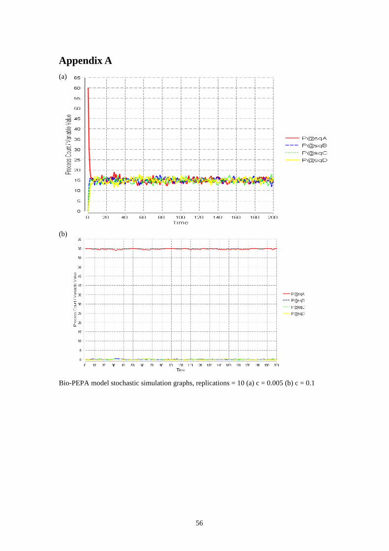
56

Appendix A (a) (b) Bio-PEPA model stochastic simulation graphs, replications = 10 (a) c = 0.005 (b) c = 0.1

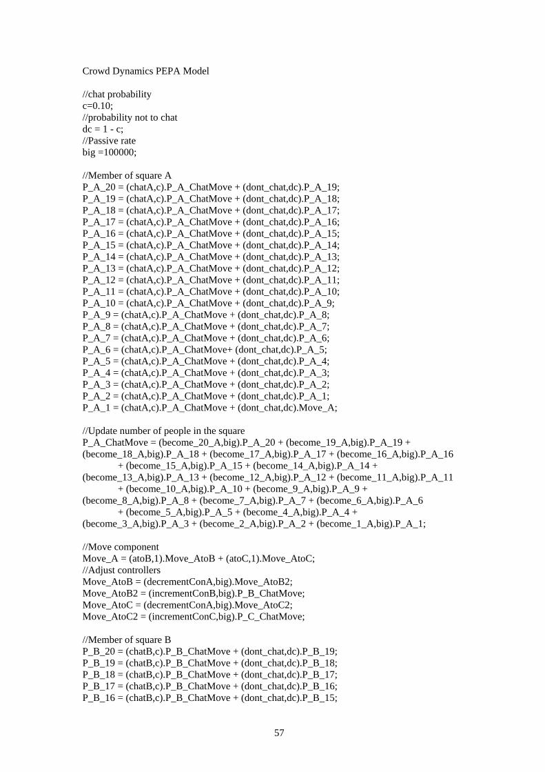
57

Crowd Dynamics PEPA Model //chat probability c=0.10; //probability not to chat dc = 1 - c; //Passive rate big =100000; //Member of square A P_A_20 = (chatA,c).P_A_ChatMove + (dont_chat,dc).P_A_19; P_A_19 = (chatA,c).P_A_ChatMove + (dont_chat,dc).P_A_18; P_A_18 = (chatA,c).P_A_ChatMove + (dont_chat,dc).P_A_17; P_A_17 = (chatA,c).P_A_ChatMove + (dont_chat,dc).P_A_16; P_A_16 = (chatA,c).P_A_ChatMove + (dont_chat,dc).P_A_15; P_A_15 = (chatA,c).P_A_ChatMove + (dont_chat,dc).P_A_14; P_A_14 = (chatA,c).P_A_ChatMove + (dont_chat,dc).P_A_13; P_A_13 = (chatA,c).P_A_ChatMove + (dont_chat,dc).P_A_12; P_A_12 = (chatA,c).P_A_ChatMove + (dont_chat,dc).P_A_11; P_A_11 = (chatA,c).P_A_ChatMove + (dont_chat,dc).P_A_10; P_A_10 = (chatA,c).P_A_ChatMove + (dont_chat,dc).P_A_9; P_A_9 = (chatA,c).P_A_ChatMove + (dont_chat,dc).P_A_8; P_A_8 = (chatA,c).P_A_ChatMove + (dont_chat,dc).P_A_7; P_A_7 = (chatA,c).P_A_ChatMove + (dont_chat,dc).P_A_6; P_A_6 = (chatA,c).P_A_ChatMove+ (dont_chat,dc).P_A_5; P_A_5 = (chatA,c).P_A_ChatMove + (dont_chat,dc).P_A_4; P_A_4 = (chatA,c).P_A_ChatMove + (dont_chat,dc).P_A_3; P_A_3 = (chatA,c).P_A_ChatMove + (dont_chat,dc).P_A_2; P_A_2 = (chatA,c).P_A_ChatMove + (dont_chat,dc).P_A_1; P_A_1 = (chatA,c).P_A_ChatMove + (dont_chat,dc).Move_A; //Update number of people in the square P_A_ChatMove = (become_20_A,big).P_A_20 + (become_19_A,big).P_A_19 + (become_18_A,big).P_A_18 + (become_17_A,big).P_A_17 + (become_16_A,big).P_A_16 + (become_15_A,big).P_A_15 + (become_14_A,big).P_A_14 + (become_13_A,big).P_A_13 + (become_12_A,big).P_A_12 + (become_11_A,big).P_A_11 + (become_10_A,big).P_A_10 + (become_9_A,big).P_A_9 + (become_8_A,big).P_A_8 + (become_7_A,big).P_A_7 + (become_6_A,big).P_A_6 + (become_5_A,big).P_A_5 + (become_4_A,big).P_A_4 + (become_3_A,big).P_A_3 + (become_2_A,big).P_A_2 + (become_1_A,big).P_A_1; //Move component Move_A = (atoB,1).Move_AtoB + (atoC,1).Move_AtoC; //Adjust controllers Move_AtoB = (decrementConA,big).Move_AtoB2; Move_AtoB2 = (incrementConB,big).P_B_ChatMove; Move_AtoC = (decrementConA,big).Move_AtoC2; Move_AtoC2 = (incrementConC,big).P_C_ChatMove; //Member of square B P_B_20 = (chatB,c).P_B_ChatMove + (dont_chat,dc).P_B_19; P_B_19 = (chatB,c).P_B_ChatMove + (dont_chat,dc).P_B_18; P_B_18 = (chatB,c).P_B_ChatMove + (dont_chat,dc).P_B_17; P_B_17 = (chatB,c).P_B_ChatMove + (dont_chat,dc).P_B_16; P_B_16 = (chatB,c).P_B_ChatMove + (dont_chat,dc).P_B_15;

58

P_B_15 = (chatB,c).P_B_ChatMove + (dont_chat,dc).P_B_14; P_B_14 = (chatB,c).P_B_ChatMove + (dont_chat,dc).P_B_13; P_B_13 = (chatB,c).P_B_ChatMove + (dont_chat,dc).P_B_12; P_B_12 = (chatB,c).P_B_ChatMove + (dont_chat,dc).P_B_11; P_B_11 = (chatB,c).P_B_ChatMove + (dont_chat,dc).P_B_10; P_B_10 = (chatB,c).P_B_ChatMove + (dont_chat,dc).P_B_9; P_B_9 = (chatB,c).P_B_ChatMove + (dont_chat,dc).P_B_8; P_B_8 = (chatB,c).P_B_ChatMove + (dont_chat,dc).P_B_7; P_B_7 = (chatB,c).P_B_ChatMove + (dont_chat,dc).P_B_6; P_B_6 = (chatB,c).P_B_ChatMove + (dont_chat,dc).P_B_5; P_B_5 = (chatB,c).P_B_ChatMove + (dont_chat,dc).P_B_4; P_B_4 = (chatB,c).P_B_ChatMove + (dont_chat,dc).P_B_3; P_B_3 = (chatB,c).P_B_ChatMove + (dont_chat,dc).P_B_2; P_B_2 = (chatB,c).P_B_ChatMove + (dont_chat,dc).P_B_1; P_B_1 = (chatB,c).P_B_ChatMove + (dont_chat,dc).Move_B; //Update number of people in the square P_B_ChatMove = (become_20_B,big).P_B_20 + (become_19_B,big).P_B_19 + (become_18_B,big).P_B_18 + (become_17_B,big).P_B_17 + (become_16_B,big).P_B_16 + (become_15_B,big).P_B_15 + (become_14_B,big).P_B_14 + (become_13_B,big).P_B_13 + (become_12_B,big).P_B_12 + (become_11_B,big).P_B_11 + (become_10_B,big).P_B_10 + (become_9_B,big).P_B_9 + (become_8_B,big).P_B_8 + (become_7_B,big).P_B_7 + (become_6_B,big).P_B_6 + (become_5_B,big).P_B_5 + (become_4_B,big).P_B_4 + (become_3_B,big).P_B_3 + (become_2_B,big).P_B_2 + (become_1_B,big).P_B_1; //Move component Move_B = (btoA,1).Move_BtoA + (btoD,1).Move_BtoD; //Adjust controllers Move_BtoA = (decrementConB,big).Move_BtoA2; Move_BtoA2 = (incrementConA,big).P_A_ChatMove; Move_BtoD = (decrementConB,big).Move_BtoD2; Move_BtoD2 = (incrementConD,big).P_D_ChatMove; //Member of square C P_C_20 = (chatC,c).P_C_ChatMove + (dont_chat,dc).P_C_19; P_C_19 = (chatC,c).P_C_ChatMove + (dont_chat,dc).P_C_18; P_C_18 = (chatC,c).P_C_ChatMove + (dont_chat,dc).P_C_17; P_C_17 = (chatC,c).P_C_ChatMove + (dont_chat,dc).P_C_16; P_C_16 = (chatC,c).P_C_ChatMove + (dont_chat,dc).P_C_15; P_C_15 = (chatC,c).P_C_ChatMove + (dont_chat,dc).P_C_14; P_C_14 = (chatC,c).P_C_ChatMove + (dont_chat,dc).P_C_13; P_C_13 = (chatC,c).P_C_ChatMove + (dont_chat,dc).P_C_12; P_C_12 = (chatC,c).P_C_ChatMove + (dont_chat,dc).P_C_11; P_C_11 = (chatC,c).P_C_ChatMove + (dont_chat,dc).P_C_10; P_C_10 = (chatC,c).P_C_ChatMove + (dont_chat,dc).P_C_9; P_C_9 = (chatC,c).P_C_ChatMove + (dont_chat,dc).P_C_8; P_C_8 = (chatC,c).P_C_ChatMove + (dont_chat,dc).P_C_7; P_C_7 = (chatC,c).P_C_ChatMove + (dont_chat,dc).P_C_6; P_C_6 = (chatC,c).P_C_ChatMove + (dont_chat,dc).P_C_5; P_C_5 = (chatC,c).P_C_ChatMove + (dont_chat,dc).P_C_4; P_C_4 = (chatC,c).P_C_ChatMove + (dont_chat,dc).P_C_3; P_C_3 = (chatC,c).P_C_ChatMove + (dont_chat,dc).P_C_2; P_C_2 = (chatC,c).P_C_ChatMove + (dont_chat,dc).P_C_1; P_C_1 = (chatC,c).P_C_ChatMove + (dont_chat,dc).Move_C;

59

//Update number of people in the square P_C_ChatMove = (become_20_C,big).P_C_20 + (become_19_C,big).P_C_19 + (become_18_C,big).P_C_18 + (become_17_C,big).P_C_17 + (become_16_C,big).P_C_16 + (become_15_C,big).P_C_15 + (become_14_C,big).P_C_14 + (become_13_C,big).P_C_13 + (become_12_C,big).P_C_12 + (become_11_C,big).P_C_11 + (become_10_C,big).P_C_10 + (become_9_C,big).P_C_9 + (become_8_C,big).P_C_8 + (become_7_C,big).P_C_7 + (become_6_C,big).P_C_6 + (become_5_C,big).P_C_5 + (become_4_C,big).P_C_4 + (become_3_C,big).P_C_3 + (become_2_C,big).P_C_2 + (become_1_C,big).P_C_1; //Move component Move_C = (ctoA,1).Move_CtoA + (ctoD,1).Move_CtoD; //Adjust controllers Move_CtoA = (decrementConC,big).Move_CtoA2; Move_CtoA2 = (incrementConA,big).P_A_ChatMove; Move_CtoD = (decrementConC,big).Move_CtoD2; Move_CtoD2 = (incrementConD,big).P_D_ChatMove; //Member of square D P_D_20 = (chatD,c).P_D_ChatMove + (dont_chat,dc).P_D_19; P_D_19 = (chatD,c).P_D_ChatMove + (dont_chat,dc).P_D_18; P_D_18 = (chatD,c).P_D_ChatMove + (dont_chat,dc).P_D_17; P_D_17 = (chatD,c).P_D_ChatMove + (dont_chat,dc).P_D_16; P_D_16 = (chatD,c).P_D_ChatMove + (dont_chat,dc).P_D_15; P_D_15 = (chatD,c).P_D_ChatMove + (dont_chat,dc).P_D_14; P_D_14 = (chatD,c).P_D_ChatMove + (dont_chat,dc).P_D_13; P_D_13 = (chatD,c).P_D_ChatMove + (dont_chat,dc).P_D_12; P_D_12 = (chatD,c).P_D_ChatMove + (dont_chat,dc).P_D_11; P_D_11 = (chatD,c).P_D_ChatMove + (dont_chat,dc).P_D_10; P_D_10 = (chatD,c).P_D_ChatMove + (dont_chat,dc).P_D_9; P_D_9 = (chatD,c).P_D_ChatMove + (dont_chat,dc).P_D_8; P_D_8 = (chatD,c).P_D_ChatMove + (dont_chat,dc).P_D_7; P_D_7 = (chatD,c).P_D_ChatMove + (dont_chat,dc).P_D_6; P_D_6 = (chatD,c).P_D_ChatMove + (dont_chat,dc).P_D_5; P_D_5 = (chatD,c).P_D_ChatMove + (dont_chat,dc).P_D_4; P_D_4 = (chatD,c).P_D_ChatMove + (dont_chat,dc).P_D_3; P_D_3 = (chatD,c).P_D_ChatMove + (dont_chat,dc).P_D_2; P_D_2 = (chatD,c).P_D_ChatMove + (dont_chat,dc).P_D_1; P_D_1 = (chatD,c).P_D_ChatMove + (dont_chat,dc).Move_D; //Update number of people in the square P_D_ChatMove = (become_20_D,big).P_D_20 + (become_19_D,big).P_D_19 + (become_18_D,big).P_D_18 + (become_17_D,big).P_D_17 + (become_16_D,big).P_D_16 + (become_15_D,big).P_D_15 + (become_14_D,big).P_D_14 + (become_13_D,big).P_D_13 + (become_12_D,big).P_D_12 + (become_11_D,big).P_D_11 + (become_10_D,big).P_D_10 + (become_9_D,big).P_D_9 + (become_8_D,big).P_D_8 + (become_7_D,big).P_D_7 + (become_6_D,big).P_D_6 + (become_5_D,big).P_D_5 + (become_4_D,big).P_D_4 + (become_3_D,big).P_D_3 + (become_2_D,big).P_D_2 + (become_1_D,big).P_D_1; //Move component Move_D = (dtoB,1).Move_DtoB + (dtoC,1).Move_DtoC; //Adjust controllers Move_DtoB = (decrementConD,big).Move_DtoB2; Move_DtoB2 = (incrementConB,big).P_B_ChatMove; Move_DtoC = (decrementConD,big).Move_DtoC2;

60

Move_DtoC2 = (incrementConC,big).P_C_ChatMove; //For communication purposes and counting the populations Beh_A = (chatA,big).Beh_A + (atoB,big).Beh_B + (atoC,big).Beh_C; Beh_B = (chatB,big).Beh_B + (btoA,big).Beh_A + (btoD,big).Beh_D; Beh_C = (chatC,big).Beh_C + (ctoA,big).Beh_A + (ctoD,big).Beh_D; Beh_D = (chatD,big).Beh_D + (dtoB,big).Beh_B + (dtoC,big).Beh_C; //Controller for population in square A, keeps count of population in square A //Synchronizes with P_A components when they are chatting so //they chat to appropriate number of people Con_A_20= (decrementConA,big).Con_A_19 + (become_20_A,big).Con_A_20; Con_A_19= (decrementConA,big).Con_A_18 + (incrementConA,big).Con_A_20 + (become_19_A,big).Con_A_19; Con_A_18= (decrementConA,big).Con_A_17 + (incrementConA,big).Con_A_19 + (become_18_A,big).Con_A_18; Con_A_17= (decrementConA,big).Con_A_16 + (incrementConA,big).Con_A_18 + (become_17_A,big).Con_A_17; Con_A_16= (decrementConA,big).Con_A_15 + (incrementConA,big).Con_A_17 + (become_16_A,big).Con_A_16; Con_A_15= (decrementConA,big).Con_A_14 + (incrementConA,big).Con_A_16 + (become_15_A,big).Con_A_15; Con_A_14= (decrementConA,big).Con_A_13 + (incrementConA,big).Con_A_15 + (become_14_A,big).Con_A_14; Con_A_13= (decrementConA,big).Con_A_12 + (incrementConA,big).Con_A_14 + (become_13_A,big).Con_A_13; Con_A_12= (decrementConA,big).Con_A_11 + (incrementConA,big).Con_A_13 + (become_12_A,big).Con_A_12; Con_A_11= (decrementConA,big).Con_A_10 + (incrementConA,big).Con_A_12 + (become_11_A,big).Con_A_11; Con_A_10= (decrementConA,big).Con_A_9 + (incrementConA,big).Con_A_11 + (become_10_A,big).Con_A_10; Con_A_9= (decrementConA,big).Con_A_8 + (incrementConA,big).Con_A_10 + (become_9_A,big).Con_A_9; Con_A_8= (decrementConA,big).Con_A_7 + (incrementConA,big).Con_A_9 + (become_8_A,big).Con_A_8; Con_A_7= (decrementConA,big).Con_A_6 + (incrementConA,big).Con_A_8 + (become_7_A,big).Con_A_7; Con_A_6= (decrementConA,big).Con_A_5 + (incrementConA,big).Con_A_7 + (become_6_A,big).Con_A_6; Con_A_5= (decrementConA,big).Con_A_4 + (incrementConA,big).Con_A_6 +(become_5_A,big).Con_A_5; Con_A_4= (decrementConA,big).Con_A_3 + (incrementConA,big).Con_A_5 + (become_4_A,big).Con_A_4; Con_A_3= (decrementConA,big).Con_A_2 + (incrementConA,big).Con_A_4 + (become_3_A,big).Con_A_3; Con_A_2= (decrementConA,big).Con_A_1 + (incrementConA,big).Con_A_3 + (become_2_A,big).Con_A_2; Con_A_1= (decrementConA,big).Con_A_0 + (incrementConA,big).Con_A_2 + (become_1_A,big).Con_A_1; Con_A_0= (incrementConA,big).Con_A_1 ;

61

//Controller for population in square B,keeps count of population in square B //Synchronizes with P_B components when they are chatting so //they chat to appropriate number of people Con_B_20= (decrementConB,big).Con_B_19 + (become_20_B,big).Con_B_20; Con_B_19= (decrementConB,big).Con_B_18 + (incrementConB,big).Con_B_20 + (become_19_B,big).Con_B_19; Con_B_18= (decrementConB,big).Con_B_17 + (incrementConB,big).Con_B_19 +(become_18_B,big).Con_B_18; Con_B_17= (decrementConB,big).Con_B_16 + (incrementConB,big).Con_B_18 + (become_17_B,big).Con_B_17; Con_B_16= (decrementConB,big).Con_B_15 + (incrementConB,big).Con_B_17 + (become_16_B,big).Con_B_16; Con_B_15= (decrementConB,big).Con_B_14 + (incrementConB,big).Con_B_16 + (become_15_B,big).Con_B_15; Con_B_14= (decrementConB,big).Con_B_13 + (incrementConB,big).Con_B_15 +(become_14_B,big).Con_B_14; Con_B_13= (decrementConB,big).Con_B_12 + (incrementConB,big).Con_B_14 + (become_13_B,big).Con_B_13; Con_B_12= (decrementConB,big).Con_B_11 + (incrementConB,big).Con_B_13 + (become_12_B,big).Con_B_12; Con_B_11= (decrementConB,big).Con_B_10 + (incrementConB,big).Con_B_12 + (become_11_B,big).Con_B_11; Con_B_10= (decrementConB,big).Con_B_9 + (incrementConB,big).Con_B_11 + (become_10_B,big).Con_B_10; Con_B_9= (decrementConB,big).Con_B_8 + (incrementConB,big).Con_B_10 + (become_9_B,big).Con_B_9; Con_B_8= (decrementConB,big).Con_B_7 + (incrementConB,big).Con_B_9 + (become_8_B,big).Con_B_8; Con_B_7= (decrementConB,big).Con_B_6 + (incrementConB,big).Con_B_8 +(become_7_B,big).Con_B_7; Con_B_6= (decrementConB,big).Con_B_5 + (incrementConB,big).Con_B_7 + (become_6_B,big).Con_B_6; Con_B_5= (decrementConB,big).Con_B_4 + (incrementConB,big).Con_B_6 + (become_5_B,big).Con_B_5; Con_B_4= (decrementConB,big).Con_B_3 + (incrementConB,big).Con_B_5 + (become_4_B,big).Con_B_4; Con_B_3= (decrementConB,big).Con_B_2 + (incrementConB,big).Con_B_4 + (become_3_B,big).Con_B_3; Con_B_2= (decrementConB,big).Con_B_1 + (incrementConB,big).Con_B_3 + (become_2_B,big).Con_B_2; Con_B_1= (decrementConB,big).Con_B_0 + (incrementConB,big).Con_B_2 + (become_1_B,big).Con_B_1; Con_B_0= (incrementConB,big).Con_B_1 ; //Controller for population in square C, keeps count of population in square C //Synchronizes with P_C components when they are chatting so //they chat to appropriate number of people Con_C_20= (decrementConC,big).Con_C_19 + (become_20_C,big).Con_C_20; Con_C_19= (decrementConC,big).Con_C_18 + (incrementConC,big).Con_C_20 + (become_19_C,big).Con_C_19; Con_C_18= (decrementConC,big).Con_C_17 + (incrementConC,big).Con_C_19 +(become_18_C,big).Con_C_18; Con_C_17= (decrementConC,big).Con_C_16 + (incrementConC,big).Con_C_18 + (become_17_C,big).Con_C_17;

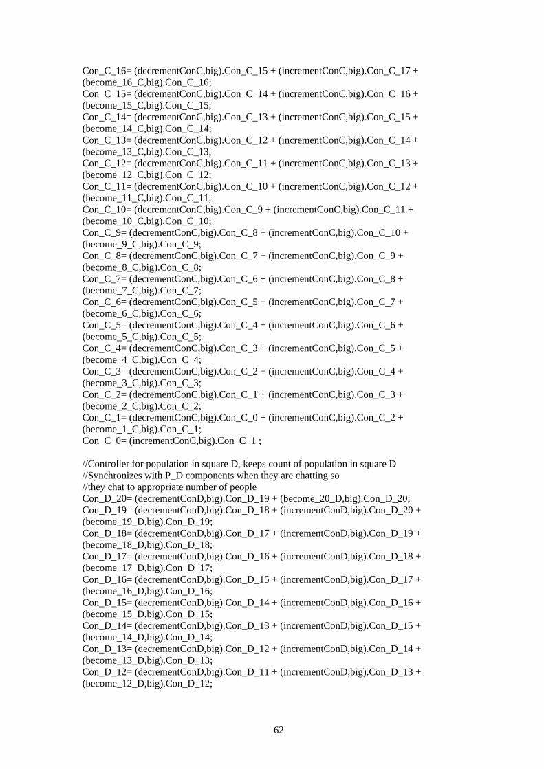
62

Con_C_16= (decrementConC,big).Con_C_15 + (incrementConC,big).Con_C_17 + (become_16_C,big).Con_C_16; Con_C_15= (decrementConC,big).Con_C_14 + (incrementConC,big).Con_C_16 + (become_15_C,big).Con_C_15; Con_C_14= (decrementConC,big).Con_C_13 + (incrementConC,big).Con_C_15 + (become_14_C,big).Con_C_14; Con_C_13= (decrementConC,big).Con_C_12 + (incrementConC,big).Con_C_14 + (become_13_C,big).Con_C_13; Con_C_12= (decrementConC,big).Con_C_11 + (incrementConC,big).Con_C_13 + (become_12_C,big).Con_C_12; Con_C_11= (decrementConC,big).Con_C_10 + (incrementConC,big).Con_C_12 + (become_11_C,big).Con_C_11; Con_C_10= (decrementConC,big).Con_C_9 + (incrementConC,big).Con_C_11 + (become_10_C,big).Con_C_10; Con_C_9= (decrementConC,big).Con_C_8 + (incrementConC,big).Con_C_10 + (become_9_C,big).Con_C_9; Con_C_8= (decrementConC,big).Con_C_7 + (incrementConC,big).Con_C_9 + (become_8_C,big).Con_C_8; Con_C_7= (decrementConC,big).Con_C_6 + (incrementConC,big).Con_C_8 + (become_7_C,big).Con_C_7; Con_C_6= (decrementConC,big).Con_C_5 + (incrementConC,big).Con_C_7 + (become_6_C,big).Con_C_6; Con_C_5= (decrementConC,big).Con_C_4 + (incrementConC,big).Con_C_6 + (become_5_C,big).Con_C_5; Con_C_4= (decrementConC,big).Con_C_3 + (incrementConC,big).Con_C_5 + (become_4_C,big).Con_C_4; Con_C_3= (decrementConC,big).Con_C_2 + (incrementConC,big).Con_C_4 + (become_3_C,big).Con_C_3; Con_C_2= (decrementConC,big).Con_C_1 + (incrementConC,big).Con_C_3 + (become_2_C,big).Con_C_2; Con_C_1= (decrementConC,big).Con_C_0 + (incrementConC,big).Con_C_2 + (become_1_C,big).Con_C_1; Con_C_0= (incrementConC,big).Con_C_1 ; //Controller for population in square D, keeps count of population in square D //Synchronizes with P_D components when they are chatting so //they chat to appropriate number of people Con_D_20= (decrementConD,big).Con_D_19 + (become_20_D,big).Con_D_20; Con_D_19= (decrementConD,big).Con_D_18 + (incrementConD,big).Con_D_20 + (become_19_D,big).Con_D_19; Con_D_18= (decrementConD,big).Con_D_17 + (incrementConD,big).Con_D_19 + (become_18_D,big).Con_D_18; Con_D_17= (decrementConD,big).Con_D_16 + (incrementConD,big).Con_D_18 + (become_17_D,big).Con_D_17; Con_D_16= (decrementConD,big).Con_D_15 + (incrementConD,big).Con_D_17 + (become_16_D,big).Con_D_16; Con_D_15= (decrementConD,big).Con_D_14 + (incrementConD,big).Con_D_16 + (become_15_D,big).Con_D_15; Con_D_14= (decrementConD,big).Con_D_13 + (incrementConD,big).Con_D_15 + (become_14_D,big).Con_D_14; Con_D_13= (decrementConD,big).Con_D_12 + (incrementConD,big).Con_D_14 + (become_13_D,big).Con_D_13; Con_D_12= (decrementConD,big).Con_D_11 + (incrementConD,big).Con_D_13 + (become_12_D,big).Con_D_12;

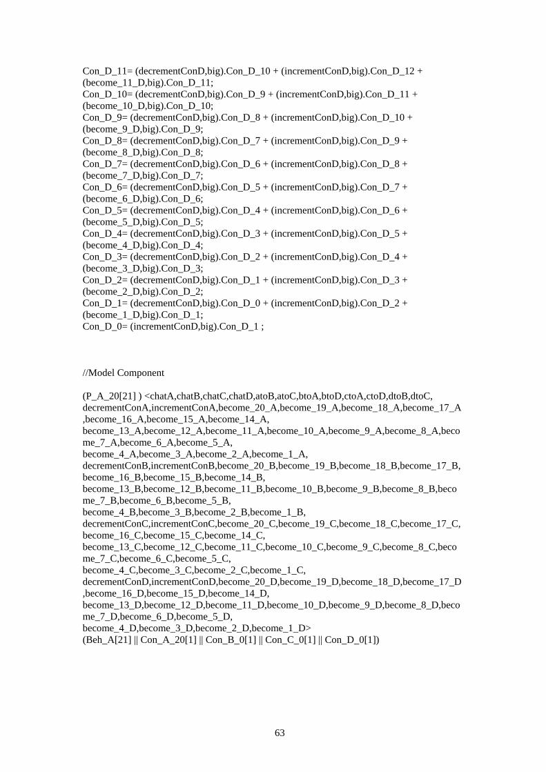
63

Con_D_11= (decrementConD,big).Con_D_10 + (incrementConD,big).Con_D_12 + (become_11_D,big).Con_D_11; Con_D_10= (decrementConD,big).Con_D_9 + (incrementConD,big).Con_D_11 + (become_10_D,big).Con_D_10; Con_D_9= (decrementConD,big).Con_D_8 + (incrementConD,big).Con_D_10 + (become_9_D,big).Con_D_9; Con_D_8= (decrementConD,big).Con_D_7 + (incrementConD,big).Con_D_9 + (become_8_D,big).Con_D_8; Con_D_7= (decrementConD,big).Con_D_6 + (incrementConD,big).Con_D_8 + (become_7_D,big).Con_D_7; Con_D_6= (decrementConD,big).Con_D_5 + (incrementConD,big).Con_D_7 + (become_6_D,big).Con_D_6; Con_D_5= (decrementConD,big).Con_D_4 + (incrementConD,big).Con_D_6 + (become_5_D,big).Con_D_5; Con_D_4= (decrementConD,big).Con_D_3 + (incrementConD,big).Con_D_5 + (become_4_D,big).Con_D_4; Con_D_3= (decrementConD,big).Con_D_2 + (incrementConD,big).Con_D_4 + (become_3_D,big).Con_D_3; Con_D_2= (decrementConD,big).Con_D_1 + (incrementConD,big).Con_D_3 + (become_2_D,big).Con_D_2; Con_D_1= (decrementConD,big).Con_D_0 + (incrementConD,big).Con_D_2 + (become_1_D,big).Con_D_1; Con_D_0= (incrementConD,big).Con_D_1 ; //Model Component (P_A_20[21] ) <chatA,chatB,chatC,chatD,atoB,atoC,btoA,btoD,ctoA,ctoD,dtoB,dtoC, decrementConA,incrementConA,become_20_A,become_19_A,become_18_A,become_17_A,become_16_A,become_15_A,become_14_A, become_13_A,become_12_A,become_11_A,become_10_A,become_9_A,become_8_A,become_7_A,become_6_A,become_5_A, become_4_A,become_3_A,become_2_A,become_1_A, decrementConB,incrementConB,become_20_B,become_19_B,become_18_B,become_17_B,become_16_B,become_15_B,become_14_B, become_13_B,become_12_B,become_11_B,become_10_B,become_9_B,become_8_B,become_7_B,become_6_B,become_5_B, become_4_B,become_3_B,become_2_B,become_1_B, decrementConC,incrementConC,become_20_C,become_19_C,become_18_C,become_17_C,become_16_C,become_15_C,become_14_C, become_13_C,become_12_C,become_11_C,become_10_C,become_9_C,become_8_C,become_7_C,become_6_C,become_5_C, become_4_C,become_3_C,become_2_C,become_1_C, decrementConD,incrementConD,become_20_D,become_19_D,become_18_D,become_17_D,become_16_D,become_15_D,become_14_D, become_13_D,become_12_D,become_11_D,become_10_D,become_9_D,become_8_D,become_7_D,become_6_D,become_5_D, become_4_D,become_3_D,become_2_D,become_1_D> (Beh_A[21] || Con_A_20[1] || Con_B_0[1] || Con_C_0[1] || Con_D_0[1])

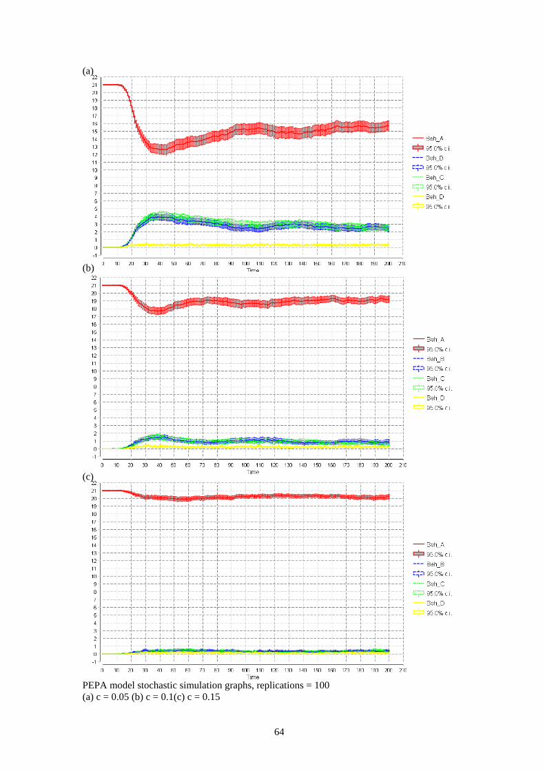
64

(a)

(b) (c) PEPA model stochastic simulation graphs, replications = 100 (a) c = 0.05 (b) c = 0.1(c) c = 0.15

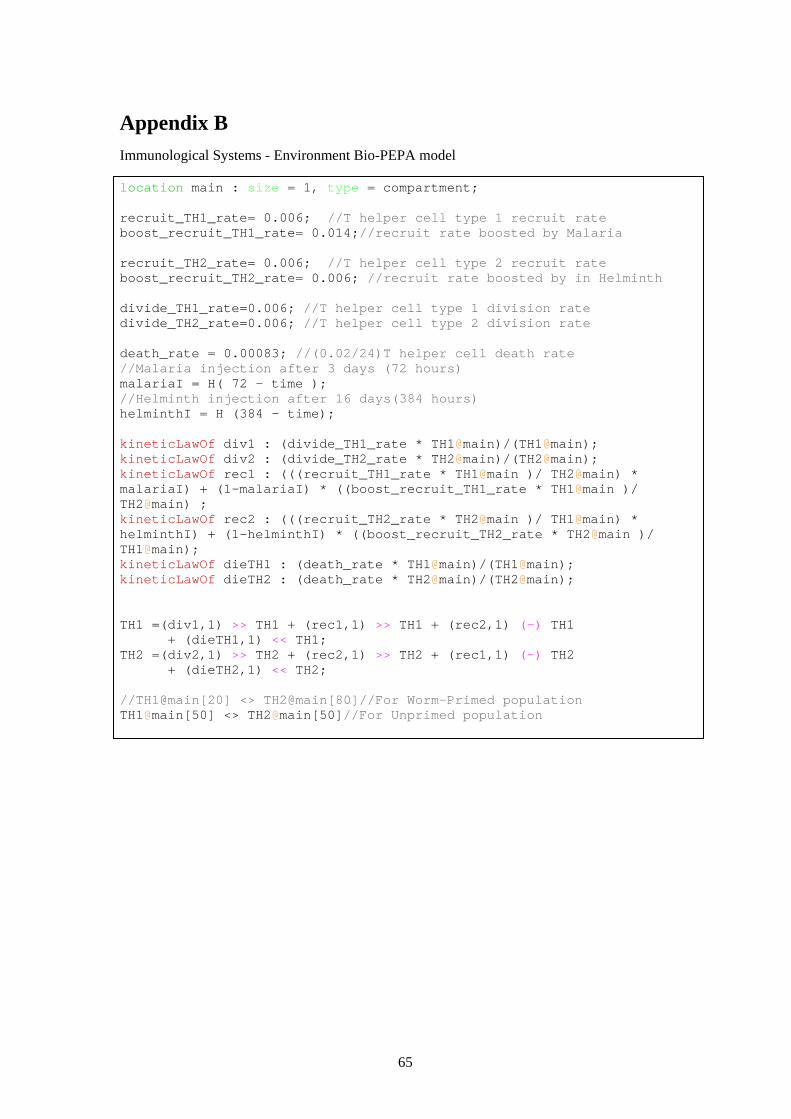
65

Appendix B Immunological Systems - Environment Bio-PEPA model

location main : size = 1, type = compartment; recruit_TH1_rate= 0.006; //T helper cell type 1 recruit rate boost_recruit_TH1_rate= 0.014;//recruit rate boosted by Malaria recruit_TH2_rate= 0.006; //T helper cell type 2 recruit rate boost_recruit_TH2_rate= 0.006; //recruit rate boosted by in Helminth divide_TH1_rate=0.006; //T helper cell type 1 division rate divide_TH2_rate=0.006; //T helper cell type 2 division rate death_rate = 0.00083; //(0.02/24)T helper cell death rate //Malaria injection after 3 days (72 hours) malariaI = H( 72 - time ); //Helminth injection after 16 days(384 hours) helminthI = H (384 - time); kineticLawOf div1 : (divide_TH1_rate * TH1@main)/(TH1@main); kineticLawOf div2 : (divide_TH2_rate * TH2@main)/(TH2@main); kineticLawOf rec1 : (((recruit_TH1_rate * TH1@main )/ TH2@main) * malariaI) + (1-malariaI) * ((boost_recruit_TH1_rate * TH1@main )/ TH2@main) ; kineticLawOf rec2 : (((recruit_TH2_rate * TH2@main )/ TH1@main) * helminthI) + (1-helminthI) * ((boost_recruit_TH2_rate * TH2@main )/ TH1@main); kineticLawOf dieTH1 : (death_rate * TH1@main)/(TH1@main); kineticLawOf dieTH2 : (death_rate * TH2@main)/(TH2@main); TH1 =(div1,1) >> TH1 + (rec1,1) >> TH1 + (rec2,1) (-) TH1 + (dieTH1,1) << TH1; TH2 =(div2,1) >> TH2 + (rec2,1) >> TH2 + (rec1,1) (-) TH2 + (dieTH2,1) << TH2; //TH1@main[20] <> TH2@main[80]//For Worm-Primed population TH1@main[50] <> TH2@main[50]//For Unprimed population

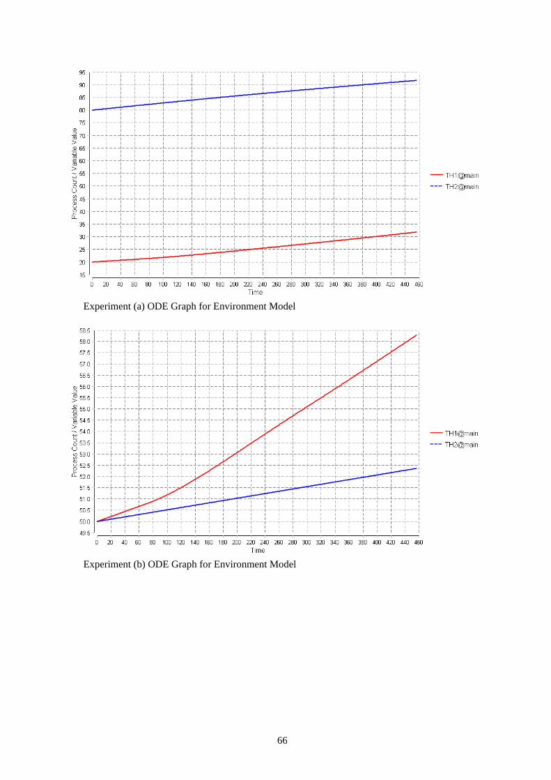
66

Experiment (a) ODE Graph for Environment Model

Experiment (b) ODE Graph for Environment Model

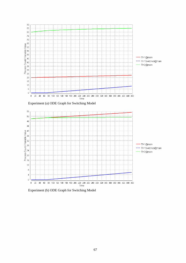
67

Experiment (a) ODE Graph for Switching Model

Experiment (b) ODE Graph for Switching Model