Embed Size (px)
Citation preview

Structural and Fluid Analysis for Large ScalePEPA Models — With Applications to Content
Adaptation Systems
Jie Ding
TH
E
U N I V E RS
I TY
OF
ED I N B U
RG
H
A thesis submitted for the degree of Doctor of Philosophy.The University of Edinburgh.
January 2010
Abstract
The stochastic process algebra PEPA is a powerful modelling formalism for concurrent sys-tems, which has enjoyed considerable success over the last decade. Such modelling can helpdesigners by allowing aspects of a system which are not readily tested, such as protocol valid-ity and performance, to be analysed before a system is deployed. However, model constructionand analysis can be challenged by the size and complexity of large scale systems, which consistof large numbers of components and thus result in state-space explosion problems. Both struc-tural and quantitative analysis of large scale PEPA models suffers from this problem, whichhas limited wider applications of the PEPA language. This thesis focuses on developing PEPA,to overcome the state-space explosion problem, and make it suitable to validate and evaluatelarge scale computer and communications systems, in particular a content adaption frameworkproposed by the Mobile VCE.
In this thesis, a new representation scheme for PEPA is proposed to numerically capture thestructural and timing information in a model. Through this numerical representation, we havefound that there is a Place/Transition structure underlying each PEPA model. Based on thisstructure and the theories developed for Petri nets, some important techniques for the struc-tural analysis of PEPA have been given. These techniques do not suffer from the state-spaceexplosion problem. They include a new method for deriving and storing the state space andan approach to finding invariants which can be used to reason qualitatively about systems. Inparticular, a novel deadlock-checking algorithm has been proposed to avoid the state-space ex-plosion problem, which can not only efficiently carry out deadlock-checking for a particularsystem but can tell when and how a system structure lead to deadlocks.
In order to avoid the state-space explosion problem encountered in the quantitative analysis ofa large scale PEPA model, a fluid approximation approach has recently been proposed, whichresults in a set of ordinary differential equations (ODEs) to approximate the underlying CTMC.This thesis presents an improved mapping from PEPA to ODEs based on the numerical repre-sentation scheme, which extends the class of PEPA models that can be subjected to fluid ap-proximation. Furthermore, we have established the fundamental characteristics of the derivedODEs, such as the existence, uniqueness, boundedness and nonnegativeness of the solution.The convergence of the solution as time tends to infinity for several classes of PEPA models,has been proved under some mild conditions. For general PEPA models, the convergence isproved under a particular condition, which has been revealed to relate to some famous con-stants of Markov chains such as the spectral gap and the Log-Sobolev constant. This thesis hasestablished the consistency between the fluid approximation and the underlying CTMCs forPEPA, i.e. the limit of the solution is consistent with the equilibrium probability distributioncorresponding to a family of underlying density dependent CTMCs.
These developments and investigations for PEPA have been applied to both qualitatively andquantitatively evaluate the large scale content adaptation system proposed by the Mobile VCE.These analyses provide an assessment of the current design and should guide the developmentof the system and contribute towards efficient working patterns and system optimisation.

Declaration of originality
I hereby declare that the research recorded in this thesis and the thesis itself was composed and
originated entirely by myself in the School of Engineering and the School of Informatics at the
University of Edinburgh.
Jie Ding
iii

Acknowledgements
First and foremost, I deeply thank my supervisors Prof. Jane Hillston and Dr David I. Lauren-
son. Without their invaluable guidance and assistance during my PhD student life, I would not
complete this thesis. I appreciate Dr Allan Clark’s help on the experiments using ipc/Hydra,
the results of which are presented in Figure 2.6 and 2.7 in this thesis.
I gratefully acknowledge the financial support from the Mobile VCE, without which I would
not have been in a position to commence and complete this work.
Finally, I am forever indebted to my parents and my sister, who have given me constant support
and encouragement. During the course of my PhD research, my mother passed away, with the
regret of having no chances to see my thesis. This thesis is in memory of my mother. Om mani
padme hum!
iv

In memory of my mother
Contents
Declaration of originality . . . . . . . . . . . . . . . . . . . . . . . . . . . . . iiiAcknowledgements . . . . . . . . . . . . . . . . . . . . . . . . . . . . . . . . ivContents . . . . . . . . . . . . . . . . . . . . . . . . . . . . . . . . . . . . . . viList of figures . . . . . . . . . . . . . . . . . . . . . . . . . . . . . . . . . . . xList of tables . . . . . . . . . . . . . . . . . . . . . . . . . . . . . . . . . . . xiiAcronyms and abbreviations . . . . . . . . . . . . . . . . . . . . . . . . . . . xiii
1 Introduction 11.1 Motivation . . . . . . . . . . . . . . . . . . . . . . . . . . . . . . . . . . . . . 11.2 Contribution of the Thesis . . . . . . . . . . . . . . . . . . . . . . . . . . . . 31.3 Organisation of the Thesis . . . . . . . . . . . . . . . . . . . . . . . . . . . . 61.4 Publication List and Some Notes . . . . . . . . . . . . . . . . . . . . . . . . . 8
2 Background 112.1 Introduction . . . . . . . . . . . . . . . . . . . . . . . . . . . . . . . . . . . . 112.2 Content Adaptation Framework by Mobile VCE . . . . . . . . . . . . . . . . . 11
2.2.1 Content adaptation . . . . . . . . . . . . . . . . . . . . . . . . . . . . 112.2.2 Mobile VCE Project . . . . . . . . . . . . . . . . . . . . . . . . . . . 132.2.3 Content adaptation framework by Mobile VCE . . . . . . . . . . . . . 132.2.4 The working cycle . . . . . . . . . . . . . . . . . . . . . . . . . . . . 15
2.3 Introduction to PEPA . . . . . . . . . . . . . . . . . . . . . . . . . . . . . . . 162.3.1 Components and activities . . . . . . . . . . . . . . . . . . . . . . . . 172.3.2 Syntax . . . . . . . . . . . . . . . . . . . . . . . . . . . . . . . . . . 182.3.3 Execution strategies, apparent rate and operational semantics . . . . . . 202.3.4 CTMC underlying PEPA model . . . . . . . . . . . . . . . . . . . . . 242.3.5 Attractive features of PEPA . . . . . . . . . . . . . . . . . . . . . . . 24
2.4 Performance Measures and Performance Evaluation for Small Scale ContentAdaptation Systems . . . . . . . . . . . . . . . . . . . . . . . . . . . . . . . . 242.4.1 PEPA model and parameter settings . . . . . . . . . . . . . . . . . . . 252.4.2 Performance measures and performance evaluation: throughput and
utilisation . . . . . . . . . . . . . . . . . . . . . . . . . . . . . . . . . 282.4.3 Performance measures and performance evaluation: response time . . . 322.4.4 Enhancing PEPA to evaluate large scale content adaptation systems . . 36
2.5 Related work . . . . . . . . . . . . . . . . . . . . . . . . . . . . . . . . . . . 372.5.1 Decomposition technique . . . . . . . . . . . . . . . . . . . . . . . . . 372.5.2 Tensor representation technique . . . . . . . . . . . . . . . . . . . . . 402.5.3 Abstraction and stochastic bound techniques . . . . . . . . . . . . . . 412.5.4 Fluid approximation technique . . . . . . . . . . . . . . . . . . . . . . 41
2.6 Summary . . . . . . . . . . . . . . . . . . . . . . . . . . . . . . . . . . . . . 44
3 New Representation for PEPA: from Syntactical to Numerical 453.1 Introduction . . . . . . . . . . . . . . . . . . . . . . . . . . . . . . . . . . . . 45
vi
Contents
3.2 Numerical Vector Form . . . . . . . . . . . . . . . . . . . . . . . . . . . . . . 463.2.1 State-space explosion problem: an illustration by a tiny example . . . . 463.2.2 Definition of numerical vector form . . . . . . . . . . . . . . . . . . . 473.2.3 Efficiency of numerical vector form . . . . . . . . . . . . . . . . . . . 493.2.4 Model 1 continued . . . . . . . . . . . . . . . . . . . . . . . . . . . . 51
3.3 Labelled Activity and Activity Matrix . . . . . . . . . . . . . . . . . . . . . . 533.3.1 Original definition of activity matrix . . . . . . . . . . . . . . . . . . . 533.3.2 Labelled activity and modified activity matrix . . . . . . . . . . . . . . 55
3.4 Transition Rate Function . . . . . . . . . . . . . . . . . . . . . . . . . . . . . 613.4.1 Model 2 continued . . . . . . . . . . . . . . . . . . . . . . . . . . . . 613.4.2 Definitions of transition rate function . . . . . . . . . . . . . . . . . . 633.4.3 Algorithm for deriving activity matrix and transition rate functions . . . 65
3.5 Associated Methods for Qualitative and Quantitative Analysis of PEPA Models 683.5.1 Numerical and aggregated representation for PEPA . . . . . . . . . . . 683.5.2 Place/Transition system . . . . . . . . . . . . . . . . . . . . . . . . . 693.5.3 Aggregated CTMC and ODEs . . . . . . . . . . . . . . . . . . . . . . 70
3.6 Summary . . . . . . . . . . . . . . . . . . . . . . . . . . . . . . . . . . . . . 72
4 Structural Analysis for PEPA Models 734.1 Introduction . . . . . . . . . . . . . . . . . . . . . . . . . . . . . . . . . . . . 734.2 Place/Transtion Structure underlying PEPA Models . . . . . . . . . . . . . . . 74
4.2.1 Dynamics of PEPA models . . . . . . . . . . . . . . . . . . . . . . . . 744.2.2 Place/Transition Structure in PEPA Models . . . . . . . . . . . . . . . 774.2.3 Some terminology . . . . . . . . . . . . . . . . . . . . . . . . . . . . 79
4.3 Invariance in PEPA models . . . . . . . . . . . . . . . . . . . . . . . . . . . . 814.3.1 What are invariants . . . . . . . . . . . . . . . . . . . . . . . . . . . . 814.3.2 How to find invariants . . . . . . . . . . . . . . . . . . . . . . . . . . 834.3.3 Conservation law as a kind of invariance . . . . . . . . . . . . . . . . . 86
4.4 Linearisation of State Space for PEPA . . . . . . . . . . . . . . . . . . . . . . 884.4.1 Linearisation of state space . . . . . . . . . . . . . . . . . . . . . . . . 884.4.2 Example . . . . . . . . . . . . . . . . . . . . . . . . . . . . . . . . . 93
4.5 Improved Deadlock-Checking Methods for PEPA . . . . . . . . . . . . . . . . 944.5.1 Preliminary . . . . . . . . . . . . . . . . . . . . . . . . . . . . . . . . 954.5.2 Equivalent deadlock-checking . . . . . . . . . . . . . . . . . . . . . . 964.5.3 Deadlock-checking algorithm in LRSPsf . . . . . . . . . . . . . . . . 984.5.4 Examples . . . . . . . . . . . . . . . . . . . . . . . . . . . . . . . . . 99
4.6 Summary . . . . . . . . . . . . . . . . . . . . . . . . . . . . . . . . . . . . . 103
5 Fluid Analysis for Large Scale PEPA Models—Part I: Probabilistic Approach 1055.1 Introduction . . . . . . . . . . . . . . . . . . . . . . . . . . . . . . . . . . . . 1055.2 Fluid Approximations for PEPA Models . . . . . . . . . . . . . . . . . . . . . 106
5.2.1 Deriving ODEs from PEPA models . . . . . . . . . . . . . . . . . . . 1075.2.2 Example . . . . . . . . . . . . . . . . . . . . . . . . . . . . . . . . . 1105.2.3 Existence and uniqueness of ODE solution . . . . . . . . . . . . . . . 112
5.3 Convergence of ODE Solution: without Synchronisations . . . . . . . . . . . . 1145.3.1 Features of ODEs without synchronisations . . . . . . . . . . . . . . . 1145.3.2 Convergence and consistency for the ODEs . . . . . . . . . . . . . . . 118
vii
Contents
5.4 Relating to Density Dependent CTMCs . . . . . . . . . . . . . . . . . . . . . 1195.4.1 Density dependent Markov chains from PEPA models . . . . . . . . . 1205.4.2 Consistency between the derived ODEs and the aggregated CTMCs . . 1235.4.3 Boundedness and nonnegativeness of ODE solutions . . . . . . . . . . 124
5.5 Convergence of ODE Solution: under a Particular Condition . . . . . . . . . . 1255.6 Investigation of the Particular Condition . . . . . . . . . . . . . . . . . . . . . 129
5.6.1 An important estimation in the context of Markov kernel . . . . . . . . 1305.6.2 Investigation of the particular condition . . . . . . . . . . . . . . . . . 131
5.7 Summary . . . . . . . . . . . . . . . . . . . . . . . . . . . . . . . . . . . . . 134
6 Fluid Analysis for Large Scale PEPA Models—Part II: Analytical Approach 1376.1 Introduction . . . . . . . . . . . . . . . . . . . . . . . . . . . . . . . . . . . . 1376.2 Analytical Proof of Boundedness and Nonnegativeness . . . . . . . . . . . . . 137
6.2.1 Features of the derived ODEs . . . . . . . . . . . . . . . . . . . . . . 1386.2.2 Boundedness and nonnegativeness of solutions . . . . . . . . . . . . . 139
6.3 A Case Study on Convergence with Two Synchronisations . . . . . . . . . . . 1416.3.1 ODEs derived from an interesting model . . . . . . . . . . . . . . . . 1416.3.2 Numerical study for convergence . . . . . . . . . . . . . . . . . . . . 148
6.4 Convergence For Two Component Types and One Synchronisation (I): A Spe-cial Case . . . . . . . . . . . . . . . . . . . . . . . . . . . . . . . . . . . . . . 1516.4.1 A previous model and the derived ODE . . . . . . . . . . . . . . . . . 1516.4.2 Outline of proof . . . . . . . . . . . . . . . . . . . . . . . . . . . . . . 1536.4.3 Proofs not relying on explicit expressions . . . . . . . . . . . . . . . . 161
6.5 Convergence For Two Component Types and One Synchronisation (II): GeneralCase . . . . . . . . . . . . . . . . . . . . . . . . . . . . . . . . . . . . . . . . 1686.5.1 Features of coefficient matrix . . . . . . . . . . . . . . . . . . . . . . 1686.5.2 Eigenvalues of Q1 and Q2 . . . . . . . . . . . . . . . . . . . . . . . . 1736.5.3 Convergence theorem . . . . . . . . . . . . . . . . . . . . . . . . . . . 177
6.6 Summary . . . . . . . . . . . . . . . . . . . . . . . . . . . . . . . . . . . . . 179
7 Deriving Performance Measures for Large Scale Content Adaptation Systems 1817.1 Introduction . . . . . . . . . . . . . . . . . . . . . . . . . . . . . . . . . . . . 1817.2 Fluid Approximation of the PEPA Model of Content Adaptation Systems . . . 182
7.2.1 ODEs derived from the PEPA model of content adaptation systems . . 1827.2.2 The properties of the solution of the derived ODEs . . . . . . . . . . . 185
7.3 Deriving Quantitative Performance Measures through Different Approaches . . 1927.3.1 Deriving performance measures through fluid approximation approach . 1927.3.2 Deriving average response time via Little’s Law . . . . . . . . . . . . . 1967.3.3 Deriving performance measures through stochastic simulation approach 1977.3.4 Comparison of performance measures through different approaches . . 201
7.4 Performance Analysis for Large Scale Content Adaptation Systems . . . . . . 2077.4.1 Scalability analysis . . . . . . . . . . . . . . . . . . . . . . . . . . . . 2097.4.2 Capacity planning . . . . . . . . . . . . . . . . . . . . . . . . . . . . 2107.4.3 Sensitivity analysis . . . . . . . . . . . . . . . . . . . . . . . . . . . . 212
7.5 Structural Analysis of A Subsystem . . . . . . . . . . . . . . . . . . . . . . . 2157.5.1 Adaptation management model . . . . . . . . . . . . . . . . . . . . . 2157.5.2 Invariants . . . . . . . . . . . . . . . . . . . . . . . . . . . . . . . . . 217
viii
Contents
7.5.3 Deadlock-checking . . . . . . . . . . . . . . . . . . . . . . . . . . . . 2207.6 Summary . . . . . . . . . . . . . . . . . . . . . . . . . . . . . . . . . . . . . 220
8 Conclusions 2238.1 Introduction . . . . . . . . . . . . . . . . . . . . . . . . . . . . . . . . . . . . 2238.2 Summary . . . . . . . . . . . . . . . . . . . . . . . . . . . . . . . . . . . . . 2238.3 Limitations of the thesis and Future work . . . . . . . . . . . . . . . . . . . . 226
References 229
A From Process Algebra to Stochastic Process Algebra 243A.1 Process algebra . . . . . . . . . . . . . . . . . . . . . . . . . . . . . . . . . . 243A.2 Timed process algebra . . . . . . . . . . . . . . . . . . . . . . . . . . . . . . 244A.3 Probabilistic process algebra . . . . . . . . . . . . . . . . . . . . . . . . . . . 245A.4 Stochastic process algebra . . . . . . . . . . . . . . . . . . . . . . . . . . . . 245
B Two Proofs in Chapter 3 247B.1 Proof of consistency between transition rate function and PEPA semantics . . . 247B.2 Proof of Proposition 3.4.3 . . . . . . . . . . . . . . . . . . . . . . . . . . . . . 248
C Some Theorems and Functional Analysis of Markov chains 251C.1 Some theorems . . . . . . . . . . . . . . . . . . . . . . . . . . . . . . . . . . 251C.2 Spectral gaps and Log-Sobolev constants of Markov chains . . . . . . . . . . . 252
D Proofs and Some Background Theories in Chapter 6 257D.1 Some basic results in mathematical analysis . . . . . . . . . . . . . . . . . . . 257D.2 Some theories of differential equations . . . . . . . . . . . . . . . . . . . . . . 258
D.2.1 The Jordan Canonical Form . . . . . . . . . . . . . . . . . . . . . . . 258D.2.2 Some obtained results . . . . . . . . . . . . . . . . . . . . . . . . . . 261
D.3 Eigenvalue properties of coefficient matrices of Model 3 . . . . . . . . . . . . 264D.4 Eigenvalue property for more general cases . . . . . . . . . . . . . . . . . . . 265D.5 A proof of (6.42) in Section 6.4.2.2 . . . . . . . . . . . . . . . . . . . . . . . . 266D.6 A proof of Lemma 6.4.1 . . . . . . . . . . . . . . . . . . . . . . . . . . . . . 270
ix
List of figures
1.1 A diagram of the work for PEPA . . . . . . . . . . . . . . . . . . . . . . . . . 41.2 Reading order of chapters . . . . . . . . . . . . . . . . . . . . . . . . . . . . . 8
2.1 Logical architecture of content adaptation framework . . . . . . . . . . . . . . 142.2 Working cycle of content adaptation management . . . . . . . . . . . . . . . . 162.3 Operational semantics of PEPA . . . . . . . . . . . . . . . . . . . . . . . . . . 232.4 Throughput of the CA adaptation ((M,N,P, Q) = 1) . . . . . . . . . . . . . . 302.5 Utilisation of the CA . . . . . . . . . . . . . . . . . . . . . . . . . . . . . . . 312.6 Response time as a function of adaptation rate and AM decision rate . . . . . . 342.7 Response time changes with the number of PDEs . . . . . . . . . . . . . . . . 352.8 Throughput and utilisation changes with the number of PDEs . . . . . . . . . . 352.9 Adaptation rate and the number of PDEs’ impact on the system performance . 35
3.1 Transition between states (Model 1) . . . . . . . . . . . . . . . . . . . . . . . 523.2 Transition vectors form an activity matrix (Model 1) . . . . . . . . . . . . . . 543.3 Transition diagram of Model 2 . . . . . . . . . . . . . . . . . . . . . . . . . . 56
4.1 Transition diagram of Model 1 (M = N = 2) . . . . . . . . . . . . . . . . . . 754.2 Transition systems of the components of Model 3 . . . . . . . . . . . . . . . . 82
5.1 Transition diagram of Model 2 . . . . . . . . . . . . . . . . . . . . . . . . . . 1105.2 Transition diagram of Model 5 . . . . . . . . . . . . . . . . . . . . . . . . . . 1175.3 Convergence and consistency diagram for derived ODEs . . . . . . . . . . . . 128
6.1 Transition systems of the components of Model 3 . . . . . . . . . . . . . . . . 1426.2 Numerical study for Model 3: rates (1, 1, 1, 1, 1, 1) . . . . . . . . . . . . . . . 1486.3 Numerical study for Model 3: rates (1, 1, 1, 10, 1, 10) . . . . . . . . . . . . . . 1496.4 Numerical study for Model 3: rates (1, 1, 10, 1, 1, 1) . . . . . . . . . . . . . . . 1496.5 Numerical study for Model 3: rates (20, 20, 1, 1, 1, 1) . . . . . . . . . . . . . . 1506.6 Illustration of derived ODEs with component types and one synchronisation . . 170
7.1 Concentrated density dependent CTMCs (concentration level one) approximatethe ODEs . . . . . . . . . . . . . . . . . . . . . . . . . . . . . . . . . . . . . 187
7.2 Concentrated density dependent CTMCs (concentration level two) approximatethe ODEs . . . . . . . . . . . . . . . . . . . . . . . . . . . . . . . . . . . . . 188
7.3 Concentrated density dependent CTMCs approximate the ODEs ((M,N,P, Q) =(30, 20, 20, 20)) . . . . . . . . . . . . . . . . . . . . . . . . . . . . . . . . . . 189
7.4 Concentrated density dependent CTMCs approximate the ODEs ((M,N,P, Q) =(300, 20, 20, 20)) . . . . . . . . . . . . . . . . . . . . . . . . . . . . . . . . . 190
7.5 Comparison between three approaches to derive response time . . . . . . . . . 2037.6 Fluid approximation and stochastic simulation . . . . . . . . . . . . . . . . . . 2067.7 Throughput vs the number of PDEs . . . . . . . . . . . . . . . . . . . . . . . 208
x

List of figures
7.8 Impact of the number of C/S Providers on performance . . . . . . . . . . . . . 2107.9 Impact of the number of AMs on performance . . . . . . . . . . . . . . . . . . 2117.10 Impact of the number of CAs on performance . . . . . . . . . . . . . . . . . . 2127.11 Impact of assimilation rate on performance . . . . . . . . . . . . . . . . . . . 2137.12 Impact of decision rate on performance . . . . . . . . . . . . . . . . . . . . . 2137.13 Impact of adaptation rate on performance . . . . . . . . . . . . . . . . . . . . 2147.14 Working cycle of content adaption model . . . . . . . . . . . . . . . . . . . . 216
xi
List of tables
2.1 Comparison between PEPA and other paradigms . . . . . . . . . . . . . . . . 242.2 Parameter settings (unit of duration: millisecond) . . . . . . . . . . . . . . . . 28
3.1 Elapsed time of state pace derivation . . . . . . . . . . . . . . . . . . . . . . . 533.2 Originally defined activity matrix of Model 2 . . . . . . . . . . . . . . . . . . 563.3 Modified activity matrix of Model 2 . . . . . . . . . . . . . . . . . . . . . . . 573.4 From syntactical and separated to numerical and aggregated representation for
PEPA . . . . . . . . . . . . . . . . . . . . . . . . . . . . . . . . . . . . . . . 68
4.1 Activity matrix and pre activity matrix of Model 1 . . . . . . . . . . . . . . . . 754.2 Comparison between three approaches . . . . . . . . . . . . . . . . . . . . . . 794.3 P/T structure in PEPA models . . . . . . . . . . . . . . . . . . . . . . . . . . 814.4 Activity matrix of Model 3 . . . . . . . . . . . . . . . . . . . . . . . . . . . . 844.5 Elapsed time of state space derivation . . . . . . . . . . . . . . . . . . . . . . 884.6 Activity matrix and pre activity matrix of Model 4 . . . . . . . . . . . . . . . . 101
5.1 Comparison with respect to restrictions . . . . . . . . . . . . . . . . . . . . . 1085.2 Activity matrix and transition rate functions of Model 2 . . . . . . . . . . . . . 1105.3 Activity matrix and transition rate function of Model 5 . . . . . . . . . . . . . 1175.4 Activity matrix and transition rate function of Model 1 . . . . . . . . . . . . . 1225.5 Fundamental characteristics of derived ODEs from PEPA models . . . . . . . . 135
6.1 A summary for the convergence of Model 3 . . . . . . . . . . . . . . . . . . . 1486.2 Complex dynamical behaviour of Model 3: starting state (1,1,5,0,0,5) . . . . . 150
7.1 Percentage error between CTMCs and ODEs . . . . . . . . . . . . . . . . . . 1887.2 Deriving performance measures through stochastic simulation . . . . . . . . . 2007.3 Running times (sec.) of small scale experiments . . . . . . . . . . . . . . . . . 2047.4 Factors and effects on paths and performance . . . . . . . . . . . . . . . . . . 2057.5 Running time of large scale experiments . . . . . . . . . . . . . . . . . . . . . 2057.6 Activity matrix C of the sub content management model . . . . . . . . . . . . 2187.7 Invariants of the sub content management model . . . . . . . . . . . . . . . . . 219
xii
Acronyms and abbreviations
ACP Algebra of Communicating Processes
AM Adaptation Manager
CA Content Adaptor
CCS Calculus of Communicating Systems
CLS Calculus of Looping Sequences
CSP Communicating Sequential Processes
C/S Provider Content/Service Provider
CTMC continuous-time Markov chain
DME Device Management Entity
EMPA Extended Markovian Process Algebra
EQ equal conflict
FC free choice
IMC interactive Markov chains
Log-Sobolev logarithm Sobolev
LOTOS Language of Temporal Ordering Specifications
Mobile VCE the virtual centre of excellence in mobile communications
ODEs ordinary differential equations
OWL Web Ontology Language
PAA Personal Assistant Agent
PCM Personal Content Manager
PDE Personal Distributed Environment
PEPA Performance Evaluation Process Algebra
P/T Place/Transition
RCAT reversed compound agent theorem
SDEs stochastic differential equations
SOAP Simple Object Access Protocol
SSA stochastic simulation algorithm
TIPP TImed Process for Performance Evaluation
UDDI Universal Description, Discovery and Integration
xiii

Acronyms and abbreviations
WSDL Web Services Description Language
xiv
Chapter 1
Introduction
1.1 Motivation
In the new era of wireless, mobile connectivity, there has been a great increase in the hetero-
geneity of devices and network technologies. For instance, mobile terminals may significantly
vary in their software, hardware and network connectivity characteristics. Meanwhile, there
is an increased variety of services being offered to meet users’ preferences and needs, for ex-
ample, mobile TV services, and shopping services such as Ebay. The service may embody
functionality and deliver multiple content items to mobile end users in a specific manner. How-
ever, the mismatch between the diversity of content and the heterogeneity of devices presents a
research challenge [LL02b]. Content adaptation has emerged as a potential effective solution
to cope with the problem of delivering services and content to users in a variety of contexts.
The virtual centre of excellence in mobile communications (Mobile VCE) is addressing this
area in the programme entitled “Removing the Barriers to Ubiquitous Services”. The pro-
gramme has been investigating the tools and techniques essential to hiding complexity in the
heterogeneous communications environment that is becoming a reality. In particular, the work
makes use of agents that manage personal preferences, and control the adaptation of content to
meet the system requirements for a user to view content they have requested. The interaction
between the entities in the user-controlled devices and the network that is required to achieve
this then becomes a significant issue.
Performance modelling provides an important route to gaining insight about how systems will
perform both qualitatively and quantitatively. Such modelling can help designers by allowing
aspects of a system which are not readily tested, such as protocol validity and performance,
to be analysed before a system is deployed. This thesis will discuss and present a high-level
modelling formalism—the stochastic process algebra PEPA developed by Hillston [Hil96]—to
validate and evaluate the potential designs and configurations of a content adaptation framework
proposed by the Mobile VCE.
1
Introduction
Stochastic process algebras are powerful modelling formalisms for concurrent systems, which
have enjoyed considerable success over the last decade. As a process algebra, PEPA is a com-
positional description technique which allows a model of system to be developed as a number
of interacting components which undertake activities. In addition to the system description as-
pects the process algebra is equipped with techniques for manipulating and analysing models,
all implemented in tools [TDG09]. Thus analysis of the model becomes automatic once the
description is completed. In a stochastic process algebra additional information is incorporated
into the model, representing the expected duration of actions and the relative likelihood of al-
ternative behaviours. This is done by associating an exponentially distributed random variable
with each action in the model. This quantification allows quantified reasoning to be carried
out on the model. Thus, whereas a process algebra model can be analysed to assess whether
it behaves correctly, a stochastic process algebra model can be analysed both with respect to
correctness and timeliness of behaviour.
Once a PEPA model has been constructed two different analysis approaches are accessible from
the single model:
• The model may be used to derive a corresponding (discrete state) continuous time Markov
chain (CTMC) which can be solved for both transient and equilibrium behaviour, allow-
ing the calculation of measures such as expected throughput, utilisation and response
time distributions.
• Desirable properties of the system can be expressed as logical formulae which may be
automatically checked against the formal description of the system, to test whether the
property holds. This can be particularly useful in checking that protocols behave appro-
priately and that certain desired properties of the system are not violated.
However, these two basic types of analysis can be challenged by the size and complexity of
large scale systems. In fact, a realistic system may consist of large numbers of users and other
entities, which results in the size of the state space underlying the system being too large to
allow analysis. This problem is termed the state-space explosion problem. Both qualitative
and quantitative analysis of stochastic process algebras and many other formal modelling ap-
proaches suffer this problem. For instance, the current deadlock-checking algorithm of PEPA
relies on exploring the entire state space to find whether a deadlock exists. For large scale PEPA
models, deadlock-checking becomes impossible due to the state-space explosion problem.
2
Introduction
For quantitative analysis of PEPA models, a novel approach—fluid approximation—to avoid
this problem has recently been developed by Hillston [Hil05a], which results in a set of ordinary
differential equations (ODEs) to approximate the underlying CTMC. However, this approach
is restricted to a class of models and needs to be extended. Furthermore, the approach gives
rise to some fundamental theoretical questions. For example, whether the solution of the ODEs
converges to a finite limit as time tends to infinity? What is the relationship between the derived
ODEs and the underlying CTMC? etc. Solving these problems can not only bring confidence
in the new approach, but can also provide new insight into, as well as a profound understanding
of, performance formalisms.
Therefore, it is an important issue and this thesis focuses on this topic, to both technically and
theoretically develop the stochastic process algebra PEPA to overcome the state-space explo-
sion problem, and make it suitable to validate and evaluate large scale computer and communi-
cations systems, in particular the content adaption framework proposed by the Mobile VCE.
1.2 Contribution of the Thesis
In this section we outline the work which has been undertaken, highlighting the primary con-
tributions of the thesis. These include both theoretical underpinnings for large scale modelling
and an application to the evaluation of large scale content adaptation systems.
A PEPA model is constructed to approximately and abstractly represent a system while hiding
its implementation details. Based on the model, performance properties of the dynamic be-
haviour of the system can be assessed, through some techniques and computational methods.
This process is referred to as the performance modelling of the system, which mainly involves
three levels: model construction and representation, technical computation and performance
derivation. Our enhancement for PEPA embodies these three aspects, which are illustrated by
Figure 1.1. At the first level, we propose a new representation scheme to numerically describe
any given PEPA model, which provides a platform to directly employ a variety of approaches
to analyse the model. These approaches are shown at the second level. At this level, the current
fluid approximation method for the quantitative analysis of PEPA is expanded, as well as in-
vestigated, mainly with respect to its convergence and the consistency and comparison between
this method and the underlying CTMC. Moreover, a Place/Transition (P/T) structure-based ap-
proach is proposed to qualitatively analyse the model. At the third level, both qualitative and
3
Introduction
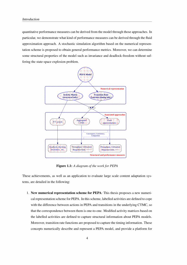
quantitative performance measures can be derived from the model through those approaches. In
particular, we demonstrate what kind of performance measures can be derived through the fluid
approximation approach. A stochastic simulation algorithm based on the numerical represen-
tation scheme is proposed to obtain general performance metrics. Moreover, we can determine
some structural properties of the model such as invariance and deadlock-freedom without suf-
fering the state-space explosion problem.
P/T system
Activity Matrix(structural info.)
Transition Rate Function (timing info.)
Fluid approximations
Aggregated CTMC
Deadlock-checkingInvariance, etc.
Throughput, Utilisation Response time, ……
Throughput, UtilisationResponse time,……
Structural and performance measures
Associated approaches
PEPA Model
Convergence, Consistency,Comparison
Numerical representation
Figure 1.1: A diagram of the work for PEPA
These achievements, as well as an application to evaluate large scale content adaptation sys-
tems, are detailed in the following:
1. New numerical representation scheme for PEPA: This thesis proposes a new numeri-
cal representation scheme for PEPA. In this scheme, labelled activities are defined to cope
with the difference between actions in PEPA and transitions in the underlying CTMC, so
that the correspondence between them is one-to-one. Modified activity matrices based on
the labelled activities are defined to capture structural information about PEPA models.
Moreover, transition rate functions are proposed to capture the timing information. These
concepts numerically describe and represent a PEPA model, and provide a platform for
4
Introduction
conveniently and easily exposing and simulating the underlying CTMC, deriving the fluid
approximation, as well as leading to an underlying P/T structure. These definitions have
been proved consistent with the original semantics of PEPA. An algorithm for automat-
ically deriving these definitions from any given PEPA model has been provided. Some
good characteristics of this numerical representation have been revealed. For example,
using numerical vector forms the exponential increase of the size of the state space with
the number of components can be reduced to at most a polynomial increase.
2. Efficient techniques for qualitative analysis of PEPA: Through the numerical represen-
tation of PEPA, we have found that there is a P/T structure underlying each PEPA model,
which reveals tight connections between stochastic process algebras and stochastic Petri
nets. Based on this structure and the theories developed for Petri nets, several powerful
techniques and approaches for structural analysis of PEPA are proposed. For instance,
we give a method of deriving and storing the state space which avoids the problems as-
sociated with populations of components, and an approach to find invariants which can
be used to qualitatively reason about systems. Moreover, a structure-based deadlock-
checking algorithm is proposed, which can avoid the state-space explosion problem.
3. Technical and theoretical developments of fluid-flow analysis of PEPA: Based on the
numerical representation scheme, we have proposed a new approach for the fluid approx-
imation of PEPA, which extends the current semantics of mapping PEPA models to ODEs
by relaxing previous restrictions. The derived ODEs through our approach can be con-
sidered as the limit of a family of density dependent CTMCs underlying the given PEPA
model. The fundamental characteristics of the derived ODEs have been established, in-
cluding the existence, uniqueness, boundedness and nonnegativeness of the solution. We
have revealed consistency between the deterministic ODEs and the underlying stochas-
tic CTMCs for general PEPA models: if the solution of the derived ODEs converges as
time tends to infinity, then the limit is an expectation in terms of the steady-state prob-
ability distributions of the corresponding density dependent CTMCs. The convergence
of the solution of the ODEs has been proved under a particular condition, which relates
the convergence problem to some well-known constants of Markov chains such as the
spectral gap and the Log-Sobolev constant. For several classes of PEPA models, the con-
vergence has been demonstrated under some mild conditions, and the coefficient matrices
of the derived ODEs have been exposed to have the following property: all eigenvalues
are either zeros or have negative real parts. In particular, invariants in the PEPA models
5

Introduction
have been shown to play an important role in the proof of convergence.
4. Performance derivation methods for large scale PEPA models: We have shown what
kind of performance metrics can be derived from a PEPA model through the approach of
fluid approximation and how this can be done. For the measures that cannot be derived by
this approach, we have presented a stochastic simulation algorithm which is based on the
numerical representation scheme. Detailed comparisons between these two approaches,
in terms of both computational cost and accuracy, have been provided.
5. Performance validation and evaluation framework for large scale content adapta-
tion systems: We have proposed a formal approach as well as associated techniques
and methods to validate (e.g. check deadlocks) and evaluate content adaptation systems,
particularly at large scales. We have developed powerful techniques for future quali-
tative analysis, including qualitative reasoning techniques through invariants as well as
structure-based methods for protocol validation, and so on. Quantitative analysis, in
terms of the response time of the system, has been carried out to assess the current design.
In particular, we have shown that the average response time is approximately governed
by a set of corresponding nonlinear algebra equations, based on which scalability and
sensitivity analysis, as well as capacity planning and system optimisation, can be carried
out simply and efficiently.
1.3 Organisation of the Thesis
The remaining chapters of this thesis are organised as follows:
Chapter 2 (Background): This chapter will present some background to the Mobile VCE
project and an introduction to PEPA, as well as some performance analyses for small
scale content adaptation systems.
Chapter 3 (Numerical representation for PEPA): This chapter will demonstrate a numeri-
cal presentation scheme for PEPA. The definitions of labelled activities, which form
a modified activity matrix, and transition rate functions as well as their corresponding
properties will be given. Moreover, this chapter will provide an algorithm for deriving
this scheme from any PEPA model.
6
Introduction
Chapter 4 (Structural analysis for PEPA): This chapter will reveal that there is a P/T struc-
ture underlying each PEPA model. Based on this structure and the theories developed
for Petri nets, structural analysis for PEPA will be carried out. This chapter will provide
powerful methods to derive and store the state space and to find invariants in PEPA mod-
els. In particular, a new deadlock-checking approach for PEPA will be proposed, to avoid
the state-space explosion problem.
Chapter 5 (Fluid analysis for PEPA (I)—through a probabilistic approach): In this chap-
ter, an improved mapping from PEPA to ODEs will be given, which extends the cur-
rent mapping semantics by relaxing certain restrictions. Some fundamental character-
istics such as the existence and uniqueness of the solution of the derived ODEs will
be presented. For PEPA models without synchronisations, the solution of the ODEs con-
verges to a limit which coincides with the stable probability distribution of the underlying
CTMC.
Chapter 6 (Fluid analysis for PEPA (II)—through an analytic approach): This chapter will
present a purely analytical proof of the boundedness and nonnegativeness of the solution
of the derived ODEs from PEPA models. A case study will show the important role of
invariance in the proof of convergence. For a class of PEPA models, i.e. models with two
component types and one synchronisation, we will demonstrate the convergence under
some mild conditions.
Chapter 7 (Deriving performance measures for large scale content adaptation systems): In
this chapter, we will show the kind of performance measures available from the fluid ap-
proximation of a PEPA model and how these measures can be derived. A stochastic simu-
lation algorithm for deriving performance based on the numerical representation scheme
will also be presented. This chapter will present applications of enhanced PEPA to val-
idate and evaluate large scale content adaptation systems. We will carry out scalability
and sensitivity analysis, as well as capacity planning for content adaptation systems, to
assess the performance. The computational cost and accuracy of different approaches
for PEPA analysis, particularly the fluid approximation and the simulation approaches,
will be experimentally compared and studied. In addition, some structural analysis for a
subsystem will be demonstrated.
Chapter 8 (Conclusions): This chapter will conclude the thesis and propose future work.
7
Introduction
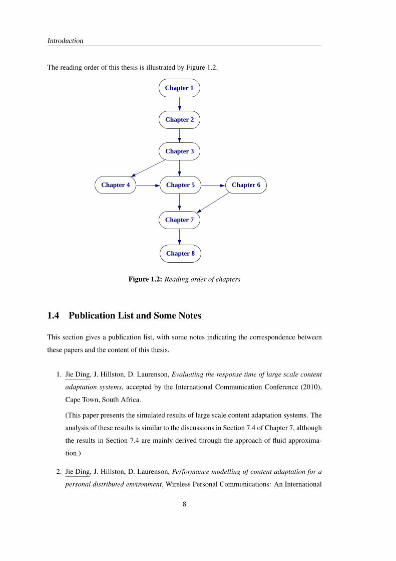
The reading order of this thesis is illustrated by Figure 1.2.
Chapter 1
Chapter 4 Chapter 5
Chapter 2
Chapter 3
Chapter 6
Chapter 7
Chapter 8
Figure 1.2: Reading order of chapters
1.4 Publication List and Some Notes
This section gives a publication list, with some notes indicating the correspondence between
these papers and the content of this thesis.
1. Jie Ding, J. Hillston, D. Laurenson, Evaluating the response time of large scale content
adaptation systems, accepted by the International Communication Conference (2010),
Cape Town, South Africa.
(This paper presents the simulated results of large scale content adaptation systems. The
analysis of these results is similar to the discussions in Section 7.4 of Chapter 7, although
the results in Section 7.4 are mainly derived through the approach of fluid approxima-
tion.)
2. Jie Ding, J. Hillston, D. Laurenson, Performance modelling of content adaptation for a
personal distributed environment, Wireless Personal Communications: An International
8

Introduction
Journal, Volume 48, Issue 1, Jan. 2009.
(This paper presents the performance modelling of a small scale content adaptation sys-
tem, in which some analysis and discussions appear in Section 2.4 of Chapter 2.)
3. Jie Ding, J. Hillston, A new deadlock checking algorithm for PEPA, 8th Workshop on
Process Algebra and Stochastically Timed Activities (PASTA’09), Edinburgh, UK.
(A brief introduction to the numerical representation scheme of PEPA and based on
which some structural analysis of PEPA models, particularly the deadlock-checking method,
have been presented in this paper. These materials are mainly shown in Chapter 3 and
Chapter 4 in this thesis.)
4. A. Attou, Jie Ding, D. Laurenson, and K. Moessner, Performance modelling and evalu-
ation of an adaptation management system, International Symposium on Performance
Evaluation of Computer and Telecommunication Systems 2008 (SPECTS’08), Edin-
burgh, UK.
(This paper presents the performance modelling and evaluation for the design of the
entity Adaptation Manager. In the interest of brevity the main content of this paper is not
included in this thesis.)
5. Jie Ding, J. Hillston, Convergence of the fluid approximations of PEPA Models, 7th
Workshop on Process Algebra and Stochastically Timed Activities (PASTA’08), Edin-
burgh, UK.
(This paper presents the relationship between the fluid approximation and the density
dependent Markov chains underlying the same PEPA model, as well as the convergence
of the solution of the derived ODEs as time goes to infinity under some conditions. These
results are mainly presented in Chapter 5.)
6. Jie Ding, J. Hillston, on ODEs from PEPA models, 6th Workshop on Process Algebra and
Stochastically Timed Activities (PASTA’07), London, UK.
(The fundamental characteristics of fluid approximation of PEPA models including the
existence, uniqueness, boundedness and nonegativeness of the solutions of the ODEs
derived from a class of PEPA models, have been established in this paper, while they are
extended in Chapter 6 in this thesis.)
9

10
Chapter 2Background
2.1 Introduction
This chapter will give an introduction to the Mobile VCE project and the stochastic process
algebra PEPA, which are shown in Section 2 and 3 respectively. Then, in Section 4, we present
performance measures and performance evaluation for small scale content adaptation systems
which are based on the content adaptation framework proposed by the Mobile VCE. A literature
review of the techniques developed to deal with the state-space explosion problem will be
presented in Section 5. Finally, we conclude this chapter in Section 6.
2.2 Content Adaptation Framework by Mobile VCE
In this section, we will give an introduction to content adaptation and the Mobile VCE project,
as well as describing a content adaptation framework proposed by the Mobile VCE.
2.2.1 Content adaptation
As networks become more sophisticated, both in terms of their underlying technology and
the applications running upon them, it is crucial that users’ expectations and requirements are
anticipated and met. In particular, users are basically not concerned with the technological
aspects of communications. However, at present, they need to be aware of a multitude of
details about equipment and benefits of one communication strategy over another, as well as
how to connect systems together to achieve the communication that they desire. As the number
of possible communication strategies increases, so does the complexity of negotiating the most
appropriate method of delivering content that the user wishes to access.
Users, requesting content from a provider, wish that content to be usable in a specific device or
devices. Currently a content provider may provide a number of formats of a particular content
to suit a selection of devices, or they may only provide a single format of the data. With the
11
Background
rapidly growing variety of devices that a user may expect to use for delivering a particular
content, providing content tailored to each device becomes an infeasible task for the content
provider [LL02a]. Thus, in order for a user, who needs the content in a different format, to be
able to make use of that content, a transformation needs to take place. In the wider context, not
only may transformation from one format to another be required, but additionally the content
may need to be modified, for example its bit-rate reduced, in order to meet quality of service
constraints. This process is called content adaptation. The adaptation, itself, may take place
within the domain of the service provider, the domain of the user, or may take place within the
network as a third party service.
Content adaptation can be defined as “the set of measures taken against a dynamically changing
context, for the purpose of maintaining a user experience of the delivered content as close to that
of the original content as possible” [Dey00]. Several techniques have been developed for con-
tent adaptation. One technique is transcoding, which changes the content coding format while
preserving the same information. For example, to reduce the bit-rate or save device storage, a
JPEG image is transcoded to PNG format. Another main technique is cross-modal adaptation.
This transforms content from one modality to another, such as text to speech adaptation. There
are other techniques for adaptation such as content recomposition for small displays [CWW07]
where, for instance, useful regions in a video or image are extracted and re-composed in an im-
age or video. Moreover, content adaptation management mechanisms have been incorporated
into content distribution networks [MBC+00,KM06,EKBS04], to minimize the interference of
adaptation with replication effectiveness [BB].
According to the location where the adaptation takes place, content adaptation techniques can
be classified into three categories [BGGW02]: provider-based, client-based, and proxy-based.
When the adaptation takes place on provider side (e.g. [MSCS99,PKP03]), the content provider
could have a central control over how the content and service are presented to users. Client-side
adaptation (e.g. [BHR+99, FAD+97]) is controlled by the end terminal. The user can impose
his preference of the final result, but adaptation is very limited due to the limitation of devices.
If adaptation occurs on a proxy site (e.g. [CEV00, FGC+97, LH05, YL03, JTW+07]), it will
reduce the complexity at the client and provider sides but may lose the advantage of end-to-end
security solutions.
In a ubiquitous environment, the adaptation should be context-aware, i.e. taking into consider-
ation context covering user location and preference, device characteristics, network conditions
12
Background
such as bandwidth, delay, QoS, content provider’s digital rights, natural environment charac-
teristics and content properties etc. As pointed out in [DLM08], context-aware application
and system design has evolved from early ad-hoc application-specific [WHFG92] or toolkit-
based [Dey00] design, to infrastructure-based design [Che04] which supports context-aware
application in distributed and heterogeneous environment. Content adaptation has been widely
acknowledged as one of the most important aspects for context-aware ubiquitous content de-
livery. The techniques of context acquisition and formatting and adaptation decision taking,
have been applied to adaptation management [MSCS99,PKP03,LH05,YL03,JTW+07]. Some
surveys on the content adaptation technologies can be found in [VCH03, Li06].
2.2.2 Mobile VCE Project
Before presenting a content adaptation framework put forward by the Mobile VCE, we first
introduce the Mobile VCE project. The Mobile VCE is the operating name of the Virtual Cen-
tre of Excellence in Mobile and Personal Communications Ltd, a collaborative partnership of
around 20 of the world’s most prominent mobile communications companies and 7 UK univer-
sities each having long standing specialist expertise in relevant areas. Mobile VCE engages in
industrially-led, long term, research in mobile and personal communications [htt].
Ubiquitous service represents a major future revenue stream for service providers, telecommu-
nication operators and pervasive technology manufacturers, since Bluetooth, WiFi, WiMAX,
UWB and more, are bringing the dream of ubiquitous access closer to reality. The “Removing
the Barriers to Ubiquitous Services” programme aims at hiding the complexity involved in the
communication of the content, and its delivery mechanism, from the user, empowering the user
to access anything, at anytime, from anywhere.
2.2.3 Content adaptation framework by Mobile VCE
This subsection introduces the content adaptation framework proposed by the Mobile VCE.
This introduction is based on the papers [Bus06, BID06, LM06]. For details, please refer to
them.
A design of a content adaptation framework for a personal distributed environment, being de-
veloped under the auspices of the Mobile VCE, has been presented in [Bus06]. The concept
of a Personal Distributed Environment (PDE), developed by the third programme of the Mo-
13
Background
Content and Service Adaptation
Personal DistributedEnvironment (PDE)
User InterfacesOutput
Modality 1
Output Modality n
Output Modality 2
PCM
PAA
Control Flow
Content Flow
DME
Content Adaptor
ADME PROFILE
REPOSITORY
CA DECISION LOGIC
Adaptation Mechanism
Adaptation Mechanism
Dispatcher
DRM
Routing
Content/Service Adaptation Manager
CONTEXT ASSIMILATION
ADAPTATION ENGINE
Content&
ServiceProvider
Figure 2.1: Logical architecture of content adaptation framework [Bus06]
bile VCE, core 3, is a user-centric view of communications in a heterogeneous environment,
and is defined as those nodes over which a user has control. At the user side, the Personal
Assistant Agent (PAA) is proposed to reduce the perceived complexity of future multi-device
personal area networks by proactively managing the modes, the functions, the applications, and
the connectivity of the user’s devices. In addition, employing the Personal Content Manager
(PCM) can effectively store content throughout the user’s environments, maximizing availabil-
ity and efficiency as well as retrieving the content in the most appropriate manner. The Device
Management Entity (DME) acts as platform for the PAA and PCM to operate over.
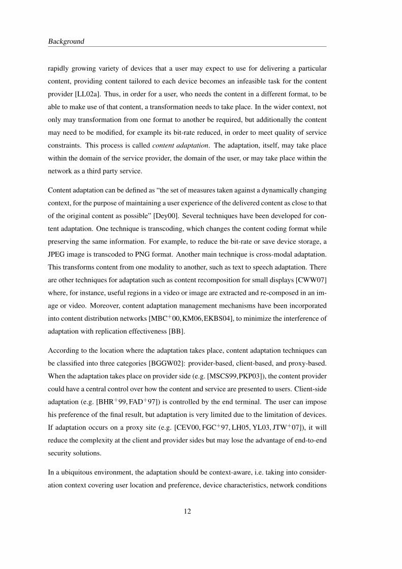
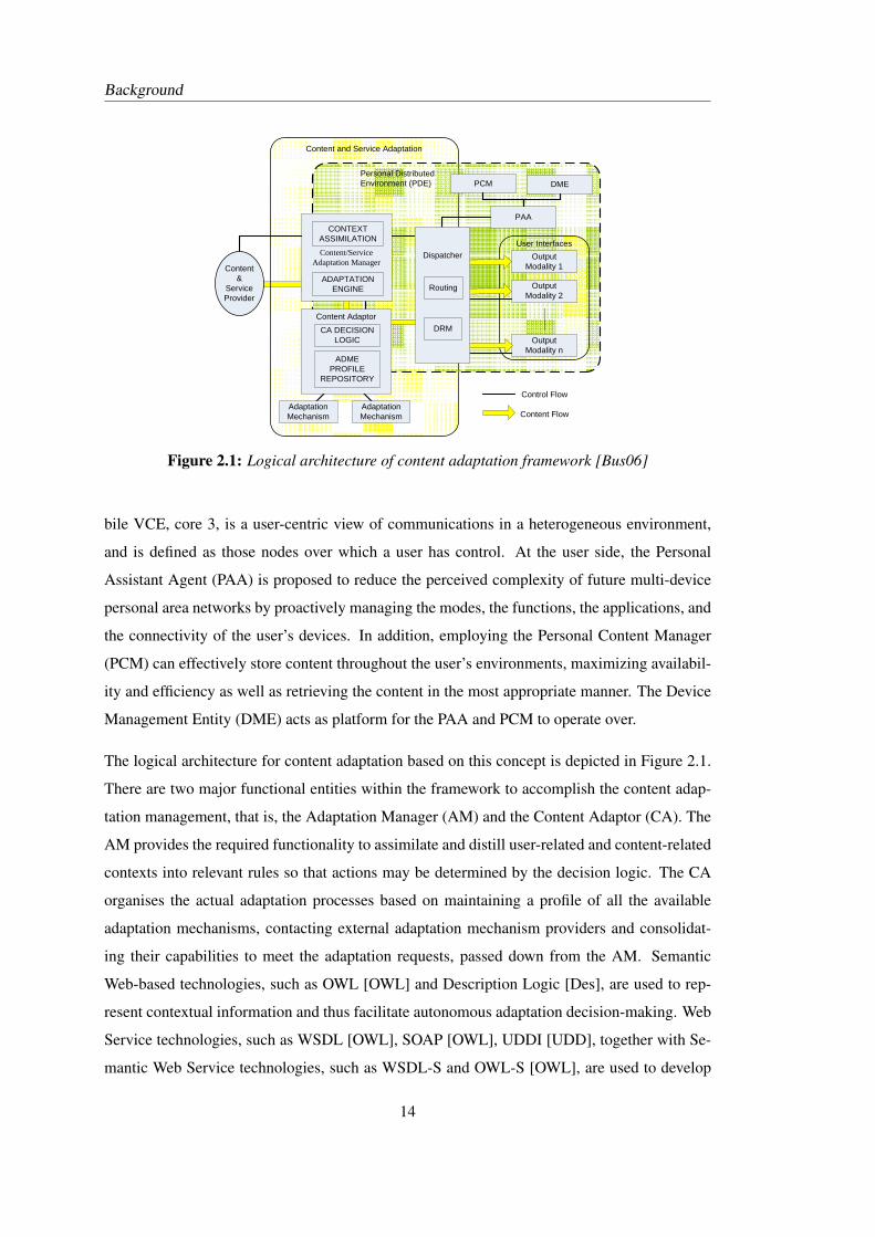
The logical architecture for content adaptation based on this concept is depicted in Figure 2.1.
There are two major functional entities within the framework to accomplish the content adap-
tation management, that is, the Adaptation Manager (AM) and the Content Adaptor (CA). The
AM provides the required functionality to assimilate and distill user-related and content-related
contexts into relevant rules so that actions may be determined by the decision logic. The CA
organises the actual adaptation processes based on maintaining a profile of all the available
adaptation mechanisms, contacting external adaptation mechanism providers and consolidat-
ing their capabilities to meet the adaptation requests, passed down from the AM. Semantic
Web-based technologies, such as OWL [OWL] and Description Logic [Des], are used to rep-
resent contextual information and thus facilitate autonomous adaptation decision-making. Web
Service technologies, such as WSDL [OWL], SOAP [OWL], UDDI [UDD], together with Se-
mantic Web Service technologies, such as WSDL-S and OWL-S [OWL], are used to develop
14
Background
adaptation mechanisms which carry out the actual content adaptation. The reader may refer
to [AM07, LM07, TBID08] for details of using these technologies within the adaptation man-
agement framework.
The Dispatcher acts as a buffer, transporting the context information from the PAA to the AM,
and delivering the content from the Content/Service Provider (C/S Provider) or the CA to the
PDE, which forms the logical interface between the personal entities and the content and service
adaptation framework as a whole.
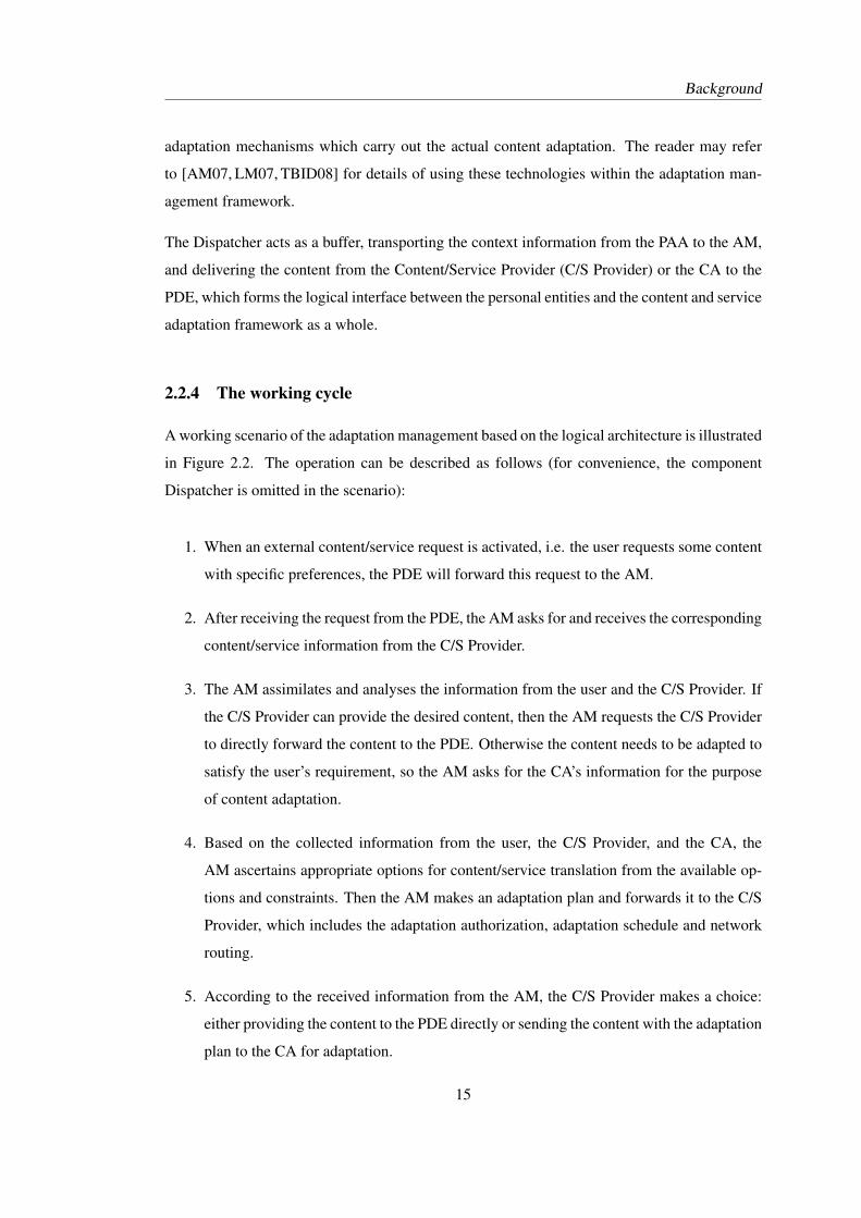
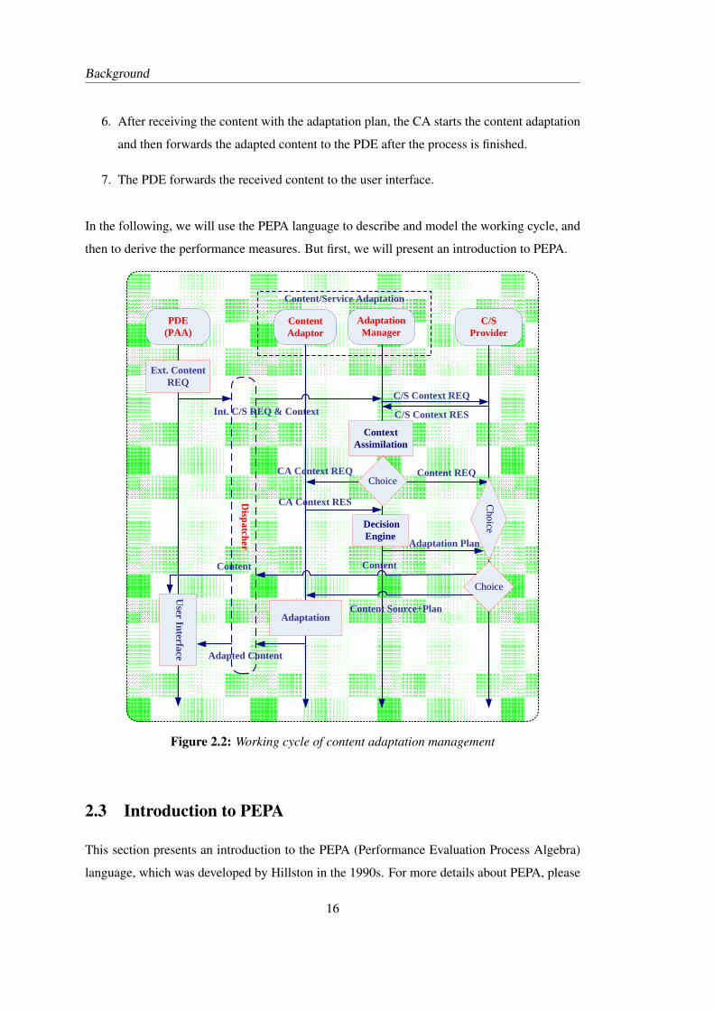
2.2.4 The working cycle
A working scenario of the adaptation management based on the logical architecture is illustrated
in Figure 2.2. The operation can be described as follows (for convenience, the component
Dispatcher is omitted in the scenario):
1. When an external content/service request is activated, i.e. the user requests some content
with specific preferences, the PDE will forward this request to the AM.
2. After receiving the request from the PDE, the AM asks for and receives the corresponding
content/service information from the C/S Provider.
3. The AM assimilates and analyses the information from the user and the C/S Provider. If
the C/S Provider can provide the desired content, then the AM requests the C/S Provider
to directly forward the content to the PDE. Otherwise the content needs to be adapted to
satisfy the user’s requirement, so the AM asks for the CA’s information for the purpose
of content adaptation.
4. Based on the collected information from the user, the C/S Provider, and the CA, the
AM ascertains appropriate options for content/service translation from the available op-
tions and constraints. Then the AM makes an adaptation plan and forwards it to the C/S
Provider, which includes the adaptation authorization, adaptation schedule and network
routing.
5. According to the received information from the AM, the C/S Provider makes a choice:
either providing the content to the PDE directly or sending the content with the adaptation
plan to the CA for adaptation.
15
Background
6. After receiving the content with the adaptation plan, the CA starts the content adaptation
and then forwards the adapted content to the PDE after the process is finished.
7. The PDE forwards the received content to the user interface.
In the following, we will use the PEPA language to describe and model the working cycle, and
then to derive the performance measures. But first, we will present an introduction to PEPA.
Content/Service Adaptation
Context Assimilation
Content REQ
Content
Content Source+Plan
Decision Engine
Dispatcher
User Interface
C/S Context REQInt. C/S REQ & Context
Adapted Content
Adaptation
PDE(PAA)
C/SProvider
Content Adaptor
AdaptationManager
C/S Context RES
Choice
Choice
Ext. Content REQ
Content
CA Context REQ
CA Context RES
Adaptation Plan
Choice
Figure 2.2: Working cycle of content adaptation management
2.3 Introduction to PEPA
This section presents an introduction to the PEPA (Performance Evaluation Process Algebra)
language, which was developed by Hillston in the 1990s. For more details about PEPA, please
16
Background
refer to [Hil96]. An overview of the history from the origin of process algebras to the current
development of stochastic process algebras (e.g. Bio-PEPA), is presented in Appendix A.
2.3.1 Components and activities
PEPA is a high-level model specification language for low-level stochastic models, which al-
lows a model of a system to be developed as a number of interacting components which un-
dertake activities. A PEPA model has a finite set of components that correspond to identifiable
parts of a system, or roles in the behaviour of the system. For example, the content adaptation
system mentioned in the previous subsection has four types of components: the PDE, the AM,
the CA and the C/S Provider. We usually use C to denote the set of all components.
The behaviour of each component in a model is captured by its activities. For instance, the
component CA can perform “ca adaptation”, i.e. the activity of content adaptation. In the
PEPA language, each activity has a type, called action type (or simply type), and a duration,
represented by activity rate (or simply rate). The duration of this activity satisfies a nega-
tive exponential distribution1 which takes the rate as its parameter. For example, the adap-
tation activity in the above example can be written as (ca adaptation, rca adaptation), where
ca adaptation is the action type and rca adaptation is the activity rate. The delay of the adap-
tation is determined by the exponential distribution with the parameter rca adaptation or with
the mean1
rca adaptation. Therefore, the probability that this activity happens within a period of
time of length t is F (t) = 1 − e−trca adaptation . The set of all action types which a component
P may next engage in is denoted byA(P ) while the multiset of all activities which P may next
fire is denoted by Act(P ). Then the sets of all possible action types and all possible activities
are written as A and Act respectively. If a component P completes an activity α ∈ A(P ) and
then behaves as a component Q, then Q is called a derivative of P and this transition can be
written as Pα→Q or P
(α,r)−→Q.
There is a special action type in PEPA, unknown type τ , which is used to represent an unknown
or unimportant action. A special activity rate in PEPA is the passive rate, denoted by >, which
is unspecified.
1In the reminder of this thesis, “negative exponential distribution” is shorted as “exponential distribution” forconvenience.
17
Background
2.3.2 Syntax
This subsection presents the name and interpretation of combinators used in the PEPA language,
which express the individual behaviours and interactions of the components.
Prefix: The prefix combinator “.” is a basic mechanism by which the first behaviour of a
component is designated. The component (α, r).P , which has action type α and a duration
which satisfies an exponential distribution with parameter r (mean 1/r), carries out the activity
(α, r) and subsequently behaves as component P . The time taken for completing the activity
will be some ∆t, sampled from the distribution.
For example, in the working cycle of the content adaptation system presented in Section 2.2.4,
a component which can launch an external content request and then behaves as PDE2, can
be expressed by (pde ext cont req , rpde ext cont req).PDE2 , where the rate rpde ext cont req re-
flects the expected rate at which the user will submit requests for the desired content or service.
We would like to denote this component by PDE1 , that is
PDE1def= (pde ext cont req , rpde ext cont req).PDE2 ,
where “def=” is another combinator which will be introduced below.
Constant: The constant combinator “def=” assigns names to components (behaviours). In the
above example, i.e., PDE1def= (pde ext cont req , rpde ext cont req).PDE2 , we assign a name
“PDE1” to the component (pde ext cont req , rpde ext cont req).PDE2 . This can also be re-
garded as the constant PDE1 being given the behaviour of the component
(pde ext cont req , rpde ext cont req).PDE2 . The constant combinator can allow infinite be-
haviour over finite states to be defined via mutually recursive definitions.
Cooperation: Interactions between components can be represented through the cooperation
combinator “ BCL
”. In fact, P BCL
Q denotes cooperation between P and Q over action types
in the cooperation set L. The cooperands are forced to synchronise on action types in L while
they can proceed independently and concurrently with other enabled activities. The rate of
the synchronised activity is determined by the slower cooperation. We write P ‖ Q as an
abbreviation for P BCL
Q when L = ∅.
In the working cycle of the content adaptation system, after the generation of the request the
next event is to pass the request to the AM. This event should be represented by a synchronous
18
Background
activity because it must be completed cooperatively by both the PDE and the AM. We use
pde int cont req to denote the action type. In the context of the PDE and the AM, the event is
respectively modelled by
PDE2def= (pde int cont req , rpde int cont req).PDE3
and
AM1def= (pde int cont req ,>).AM2 .
The cooperation between PDE2 and AM1 can be expressed by PDE2 BC{pde int cont req}
AM1.
Here the notation “>” reflects that for the AM the activity pde int cont req is passive, and the
rate is determined by its cooperation partner—the PDE. If the rate for the AM is not passive
and assigned as r, i.e., AM1def= (pde int cont req , r).AM2 , then the rate of the shared activity
pde int cont req is determined by the smaller of the two rates, i.e. min{rpde int cont req , r}.
Moreover, suppose there are two PDEs in the system and there is no cooperation between these
two PDE2. This can be modelled by PDE2 ‖ PDE2, which is equivalent to PDE2 BC∅
PDE2.
Their cooperation with the AM through the activity pde int cont req can be represented by
(PDE2 ‖ PDE2) BC{pde int cont req}
AM1. We sometimes use the notation PDE2[M ] to represent
PDE2 ‖ · · · ‖ PDE2︸ ︷︷ ︸M times
.
Choice: The choice combinator “+” expresses competition between activities. The component
P + Q models a system which may behave either as P or as Q. The activities of both P
and Q are enabled. Whichever activity completes first must belong to P or Q. This activity
distinguishes one of the components, P or Q, and the component P + Q will subsequently
behave as this component. Because of the continuous nature of the probability distributions,
the probability of P and Q both completing an activity at the same time is zero. The choice
combinator represents uncertainty about the behaviour of a component.
For example, in our content adaptation system, after forwarding the request to the AM, the PDE
waits for a response. There are two possible responses, which are represented by two possible
activities: receiving the content from the C/S Provider directly (csp to pde) or receiving the
adapted content from the CA (ca to pde). This event can be represented by
PDE3def= (csp to pde,>).PDE4 + (ca to pde,>).PDE4 .
19
Background
The rates > here reflect that for the PDE both activities are passive, and their rates are deter-
mined by their cooperation partners—the C/S Provider and the CA respectively.
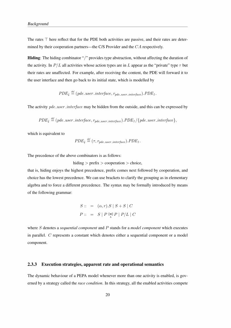
Hiding: The hiding combinator “/” provides type abstraction, without affecting the duration of
the activity. In P/L all activities whose action types are in L appear as the “private” type τ but
their rates are unaffected. For example, after receiving the content, the PDE will forward it to
the user interface and then go back to its initial state, which is modelled by
PDE4def= (pde user interface, rpde user interface).PDE1 .
The activity pde user interface may be hidden from the outside, and this can be expressed by
PDE4def= (pde user interface, rpde user interface).PDE1/{pde user interface},
which is equivalent to
PDE4def= (τ, rpde user interface).PDE1 .
The precedence of the above combinators is as follows:
hiding > prefix > cooperation > choice,
that is, hiding enjoys the highest precedence, prefix comes next followed by cooperation, and
choice has the lowest precedence. We can use brackets to clarify the grouping as in elementary
algebra and to force a different precedence. The syntax may be formally introduced by means
of the following grammar:
S :: = (α, r).S | S + S | C
P :: = S | P BCL
P | P/L | C
where S denotes a sequential component and P stands for a model component which executes
in parallel. C represents a constant which denotes either a sequential component or a model
component.
2.3.3 Execution strategies, apparent rate and operational semantics
The dynamic behaviour of a PEPA model whenever more than one activity is enabled, is gov-
erned by a strategy called the race condition. In this strategy, all the enabled activities compete
20
Background
with each other but only the fastest succeeds to proceed. The probability of an activity winning
the race is given by the ratio of the activity rate of that activity to the sum of the activity rates of
all the activities engaged in the race. This gives rise to an implicit probabilistic choice between
actions dependent of the relative values of their rates. Therefore, if a single action in a system
has more than one possible outcome, we may represent this action by more than one activity in
the corresponding PEPA model. For example, AM4 can perform the action am assimilation
with the rate ram assimilation, and then behave as AM5 or AM9, with the probabilities p and
1− p respectively. This can be modelled as:
AM4def= (am assimilation, p× ram assimilation).AM5
+ (am assimilation, (1− p)× ram assimilation).AM9 .
Here the component AM4 has two separate activities of the same action type. To an external
observer, the sum of the rates of the type am assimilation in this component will be the same,
that is ram assimilation = p × ram assimilation + (1 − p) × ram assimilation. This is called the
apparent rate of am assimilation.
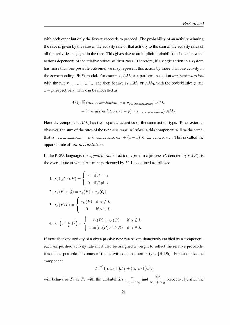
In the PEPA language, the apparent rate of action type α in a process P , denoted by rα(P ), is
the overall rate at which α can be performed by P . It is defined as follows:
1. rα((β, r).P ) =
r if β = α
0 if β 6= α
2. rα(P + Q) = rα(P ) + rα(Q)
3. rα(P/L) =
rα(P ) if α /∈ L
0 if α ∈ L
4. rα
(P BC
LQ)
=
rα(P ) + rα(Q) if α /∈ L
min(rα(P ), rα(Q)) if α ∈ L
If more than one activity of a given passive type can be simultaneously enabled by a component,
each unspecified activity rate must also be assigned a weight to reflect the relative probabili-
ties of the possible outcomes of the activities of that action type [Hil96]. For example, the
component
Pdef= (α, w1>).P1 + (α, w2>).P2
will behave as P1 or P2 with the probabilitiesw1
w1 + w2and
w2
w1 + w2respectively, after the
21
Background
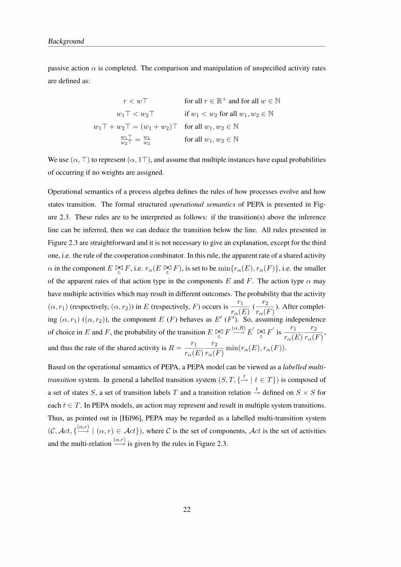
passive action α is completed. The comparison and manipulation of unspecified activity rates
are defined as:
r < w> for all r ∈ R+ and for all w ∈ N
w1> < w2> if w1 < w2 for all w1, w2 ∈ N
w1>+ w2> = (w1 + w2)> for all w1, w2 ∈ Nw1>w2> = w1
w2for all w1, w2 ∈ N
We use (α,>) to represent (α, 1>), and assume that multiple instances have equal probabilities
of occurring if no weights are assigned.
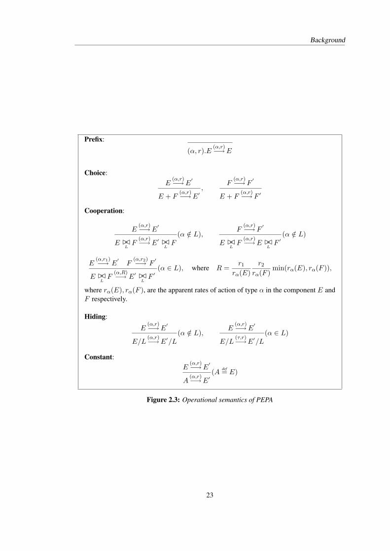
Operational semantics of a process algebra defines the rules of how processes evolve and how
states transition. The formal structured operational semantics of PEPA is presented in Fig-
ure 2.3. These rules are to be interpreted as follows: if the transition(s) above the inference
line can be inferred, then we can deduce the transition below the line. All rules presented in
Figure 2.3 are straightforward and it is not necessary to give an explanation, except for the third
one, i.e. the rule of the cooperation combinator. In this rule, the apparent rate of a shared activity
α in the component E BCL
F , i.e. rα(E BCL
F ), is set to be min{rα(E), rα(F )}, i.e. the smaller
of the apparent rates of that action type in the components E and F . The action type α may
have multiple activities which may result in different outcomes. The probability that the activity
(α, r1) (respectively, (α, r2)) in E (respectively, F ) occurs isr1
rα(E)(
r2
rα(F )). After complet-
ing (α, r1) ((α, r2)), the component E (F ) behaves as E′ (F ′). So, assuming independence
of choice in E and F , the probability of the transition E BCL
F(α,R)−→ E
′ BCL
F′
isr1
rα(E)r2
rα(F ),
and thus the rate of the shared activity is R =r1
rα(E)r2
rα(F )min(rα(E), rα(F )).
Based on the operational semantics of PEPA, a PEPA model can be viewed as a labelled multi-
transition system. In general a labelled transition system (S, T, { t→ | t ∈ T}) is composed of
a set of states S, a set of transition labels T and a transition relation t→ defined on S × S for
each t ∈ T . In PEPA models, an action may represent and result in multiple system transitions.
Thus, as pointed out in [Hil96], PEPA may be regarded as a labelled multi-transition system
(C,Act, {(α,r)−→ | (α, r) ∈ Act}), where C is the set of components, Act is the set of activities
and the multi-relation(α,r)−→ is given by the rules in Figure 2.3.
22
Background
Prefix:
(α, r).E(α,r)−→E
Choice:E
(α,r)−→E′
E + F(α,r)−→E′
,F
(α,r)−→ F′
E + F(α,r)−→ F ′
Cooperation:
E(α,r)−→E
′
E BCL
F(α,r)−→E′ BC
LF
(α /∈ L),F
(α,r)−→ F′
E BCL
F(α,r)−→E BC
LF ′
(α /∈ L)
E(α,r1)−→ E
′F
(α,r2)−→ F′
E BCL
F(α,R)−→ E′ BC
LF ′
(α ∈ L), where R =r1
rα(E)r2
rα(F )min(rα(E), rα(F )),
where rα(E), rα(F ), are the apparent rates of action of type α in the component E andF respectively.
Hiding:
E(α,r)−→E
′
E/L(α,r)−→E′/L
(α /∈ L),E
(α,r)−→E′
E/L(τ,r)−→E′/L
(α ∈ L)
Constant:E
(α,r)−→E′
A(α,r)−→E′
(A def= E)
Figure 2.3: Operational semantics of PEPA
23
Background
2.3.4 CTMC underlying PEPA model
The memoryless property of the exponential distribution, which is satisfied by the durations
of all activities, means that there is a CTMC underlying any given PEPA model [Hil96]. By
solving the matrix equation characterising the global balance equations associated with this
CTMC using linear algebra, the steady-state probability distribution can be obtained, from
which performance measures such as throughput and utilisation can be derived. Similarly the
matrix may be used as the basis for transient analysis, allowing measures such as response time
distributions to be calculated. In the next section, we will use the content adaptation example
to illustrate how to derive performance measures from a PEPA model.
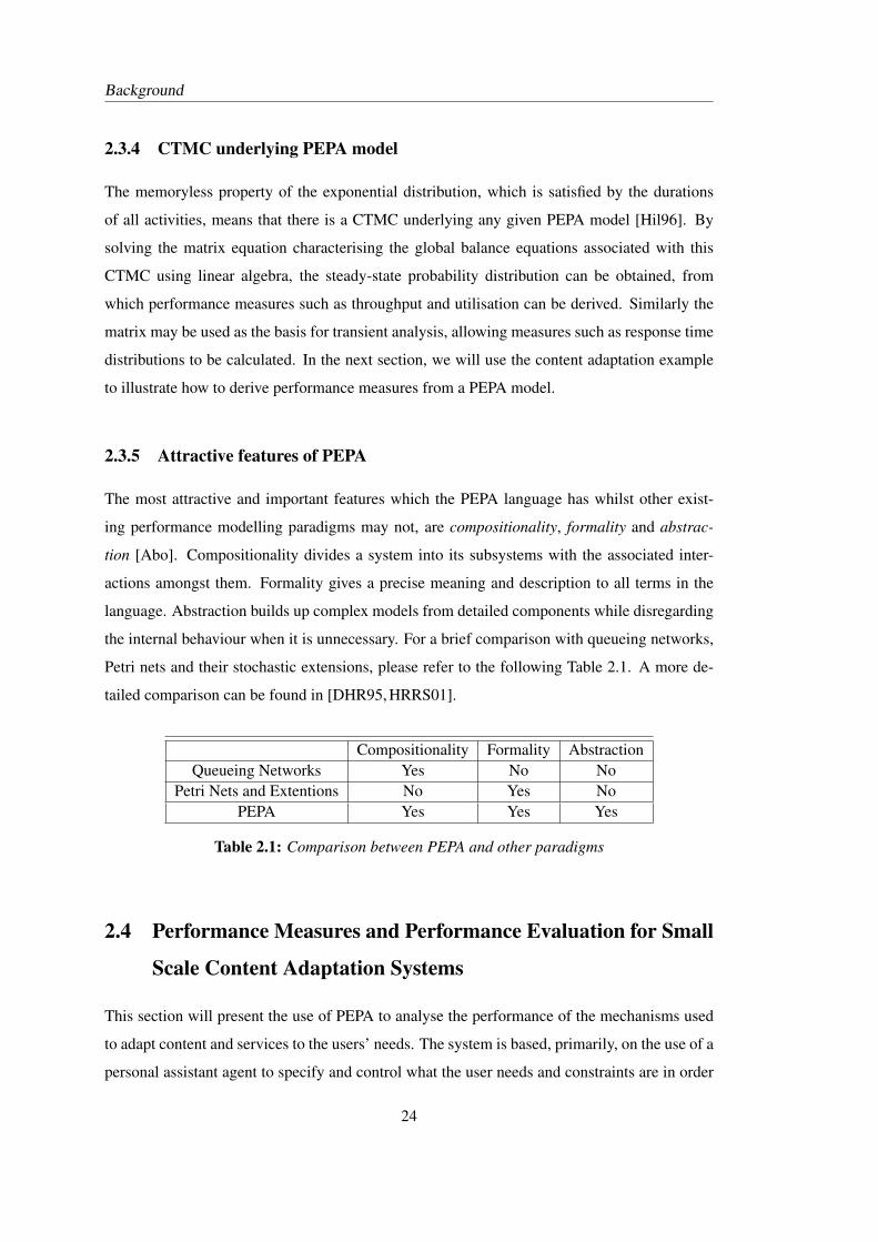
2.3.5 Attractive features of PEPA
The most attractive and important features which the PEPA language has whilst other exist-
ing performance modelling paradigms may not, are compositionality, formality and abstrac-
tion [Abo]. Compositionality divides a system into its subsystems with the associated inter-
actions amongst them. Formality gives a precise meaning and description to all terms in the
language. Abstraction builds up complex models from detailed components while disregarding
the internal behaviour when it is unnecessary. For a brief comparison with queueing networks,
Petri nets and their stochastic extensions, please refer to the following Table 2.1. A more de-
tailed comparison can be found in [DHR95, HRRS01].
Compositionality Formality AbstractionQueueing Networks Yes No No
Petri Nets and Extentions No Yes NoPEPA Yes Yes Yes
Table 2.1: Comparison between PEPA and other paradigms
2.4 Performance Measures and Performance Evaluation for Small
Scale Content Adaptation Systems
This section will present the use of PEPA to analyse the performance of the mechanisms used
to adapt content and services to the users’ needs. The system is based, primarily, on the use of a
personal assistant agent to specify and control what the user needs and constraints are in order
24
Background
to receive a particular service or content. This interacts with a content adaptation mechanism
that resides in the network. We will discuss what kind of performance measures are of interest
and how to derive these measures from the system. Performance of the system, as we will see,
depends upon an efficient negotiation, content adaptation, and delivery mechanism.
2.4.1 PEPA model and parameter settings
Based on the architecture and working cycle presented in the previous subsection, this section
defines the PEPA model of the content adaptation system. The system model is comprised of
four components, corresponding to the four major entities of the the architecture, i.e., the PDE,
the AM, the CA and the C/S Provider. Each of the components has a repetitive behaviour,
reflecting its role within the working cycle. There is no need to represent all aspects of the
components’ behaviour in detail, since the level of abstraction is chosen to be sufficient to
capture the time/resource consuming activities. Below, PEPA definitions for the components
are shown.
In Section 2.3.2, we have given the PEPA definition for the PDE. For convenience, we present
it again.
PDE: The behaviour of the PDE begins with the generation of a request for content adaptation,
represented as action pde ext cs req. The rate here reflects the expected rate at which the
user will submit requests for content adaptation. The next event is to pass the request to the
AM, pde int cs req, which is a synchronous activity. After that, the PDE waits for a response.
The model reflects that there are two possible responses, by having two possible activities:
receiving the content from the C/S Provider directly or receiving the adapted content from the
CA, which are represented by csp to pde and ca to pde respectively. The rates> here indicate
that for the PDE both activities are passive, and their rates are determined by their cooperation
partners—the C/S Provider and the CA respectively—reflecting their relative probabilities. In
each case the final action of the PDE is to send appropriate information to the user interface,
pde user interface. After completing this action, the PDE goes back to the initial state.
25
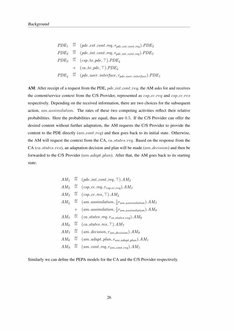
Background
PDE1def= (pde ext cont req , rpde ext cont req).PDE2
PDE2def= (pde int cont req , rpde int cont req).PDE3
PDE3def= (csp to pde,>).PDE4
+ (ca to pde,>).PDE4
PDE4def= (pde user interface, rpde user interface).PDE1
AM: After receipt of a request from the PDE, pde int cont req, the AM asks for and receives
the content/service context from the C/S Provider, represented as csp cc req and csp cc res
respectively. Depending on the received information, there are two choices for the subsequent
action, am assimilation. The rates of these two competing activities reflect their relative
probabilities. Here the probabilities are equal, thus are 0.5. If the C/S Provider can offer the
desired content without further adaptation, the AM requests the C/S Provider to provide the
content to the PDE directly (am cont req) and then goes back to its initial state. Otherwise,
the AM will request the context from the CA, ca states req. Based on the response from the
CA (ca states res), an adaptation decision and plan will be made (am decision) and then be
forwarded to the C/S Provider (am adapt plan). After that, the AM goes back to its starting
state.
AM1def= (pde int cont req ,>).AM2
AM2def= (csp cc req , rcsp cc req).AM3
AM3def= (csp cc res,>).AM4
AM4def= (am assimilation, 1
2ram assimilation).AM5
+ (am assimilation, 12ram assimilation).AM9
AM5def= (ca states req , rca states req).AM6
AM6def= (ca states res,>).AM7
AM7def= (am decision, ram decision).AM8
AM8def= (am adapt plan, ram adapt plan).AM1
AM9def= (am cont req , ram cont req).AM1
Similarly we can define the PEPA models for the CA and the C/S Provider respectively.
26
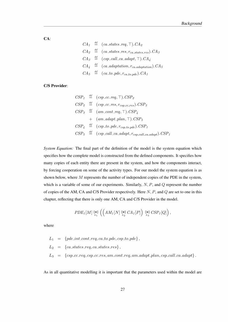
Background
CA:CA1
def= (ca states req ,>).CA2
CA2def= (ca states res, rca states res).CA3
CA3def= (csp call ca adapt ,>).CA4
CA4def= (ca adaptation, rca adaptation).CA5
CA5def= (ca to pde, rca to pde).CA1
C/S Provider:
CSP1def= (csp cc req ,>).CSP2
CSP2def= (csp cc res, rcsp cc res).CSP3
CSP3def= (am cont req ,>).CSP4
+ (am adapt plan,>).CSP5
CSP4def= (csp to pde, rcsp to pde).CSP1
CSP5def= (csp call ca adapt , rcsp call ca adapt).CSP1
System Equation: The final part of the definition of the model is the system equation which
specifies how the complete model is constructed from the defined components. It specifies how
many copies of each entity there are present in the system, and how the components interact,
by forcing cooperation on some of the activity types. For our model the system equation is as
shown below, where M represents the number of independent copies of the PDE in the system,
which is a variable of some of our experiments. Similarly, N,P , and Q represent the number
of copies of the AM, CA and C/S Provider respectively. Here N,P , and Q are set to one in this
chapter, reflecting that there is only one AM, CA and C/S Provider in the model.
PDE1 [M ] BCL1
((AM1 [N ] BC
L2CA1 [P ]
)BCL3
CSP1 [Q])
,
where
L1 = {pde int cont req, ca to pde, csp to pde} ,
L2 = {ca states req, ca states res} ,
L3 = {csp cc req, csp cc res, am cont req, am adapt plan, csp call ca adapt} .
As in all quantitative modelling it is important that the parameters used within the model are
27
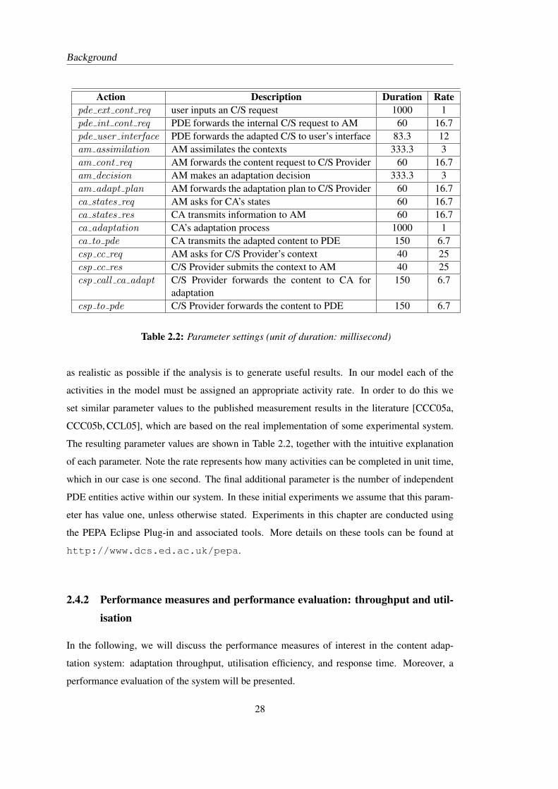
Background
Action Description Duration Ratepde ext cont req user inputs an C/S request 1000 1pde int cont req PDE forwards the internal C/S request to AM 60 16.7pde user interface PDE forwards the adapted C/S to user’s interface 83.3 12am assimilation AM assimilates the contexts 333.3 3am cont req AM forwards the content request to C/S Provider 60 16.7am decision AM makes an adaptation decision 333.3 3am adapt plan AM forwards the adaptation plan to C/S Provider 60 16.7ca states req AM asks for CA’s states 60 16.7ca states res CA transmits information to AM 60 16.7ca adaptation CA’s adaptation process 1000 1ca to pde CA transmits the adapted content to PDE 150 6.7csp cc req AM asks for C/S Provider’s context 40 25csp cc res C/S Provider submits the context to AM 40 25csp call ca adapt C/S Provider forwards the content to CA for
adaptation150 6.7
csp to pde C/S Provider forwards the content to PDE 150 6.7
Table 2.2: Parameter settings (unit of duration: millisecond)
as realistic as possible if the analysis is to generate useful results. In our model each of the
activities in the model must be assigned an appropriate activity rate. In order to do this we
set similar parameter values to the published measurement results in the literature [CCC05a,
CCC05b, CCL05], which are based on the real implementation of some experimental system.
The resulting parameter values are shown in Table 2.2, together with the intuitive explanation
of each parameter. Note the rate represents how many activities can be completed in unit time,
which in our case is one second. The final additional parameter is the number of independent
PDE entities active within our system. In these initial experiments we assume that this param-
eter has value one, unless otherwise stated. Experiments in this chapter are conducted using
the PEPA Eclipse Plug-in and associated tools. More details on these tools can be found at
http://www.dcs.ed.ac.uk/pepa.
2.4.2 Performance measures and performance evaluation: throughput and util-
isation
In the following, we will discuss the performance measures of interest in the content adap-
tation system: adaptation throughput, utilisation efficiency, and response time. Moreover, a
performance evaluation of the system will be presented.
28
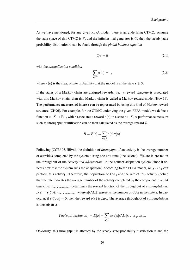
Background
As we have mentioned, for any given PEPA model, there is an underlying CTMC. Assume
the state space of this CTMC is S, and the infinitesimal generator is Q, then the steady-state
probability distribution π can be found through the global balance equation
Qπ = 0 (2.1)
with the normalisation condition ∑s∈S
π(s) = 1, (2.2)
where π(s) is the steady-state probability that the model is in the state s ∈ S.
If the states of a Markov chain are assigned rewards, i.e. a reward structure is associated
with this Markov chain, then this Markov chain is called a Markov reward model [How71].
The performance measures of interest can be represented by using this kind of Markov reward
structure [CH96]. For example, for the CTMC underlying the given PEPA model, we define a
function ρ : S → R+, which associates a reward ρ(s) to a state s ∈ S. A performance measure
such as throughput or utilisation can be then calculated as the average reward R:
R = E[ρ] =∑s∈S
ρ(s)π(s).
Following [CCE+03, Hil96], the definition of throughput of an activity is the average number
of activities completed by the system during one unit time (one second). We are interested in
the throughput of the activity “ca adaptation” in the content adaptation system, since it re-
flects how fast the system runs the adaptation. According to the PEPA model, only CA4 can
perform this activity. Therefore, the population of CA4 and the rate of this activity (notice
that the rate indicates the average number of the activity completed by the component in a unit
time), i.e. rca adaptation, determines the reward function of the throughput of ca adaptation:
ρ(s) = s[CA4]rca adaptation, where s[CA4] represents the number of CA4 in the state s. In par-
ticular, if s[CA4] = 0, then the reward ρ(s) is zero. The average throughput of ca adaptation
is thus given as:
Thr(ca adaptation) = E[ρ] =∑s∈S
π(s)s[CA4]rca adaptation.
Obviously, this throughput is affected by the steady-state probability distribution π and the
29
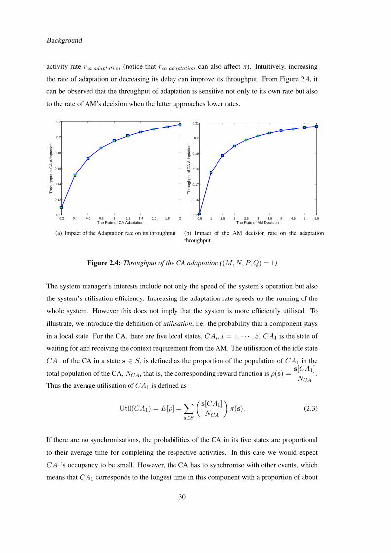
Background
activity rate rca adaptation (notice that rca adaptation can also affect π). Intuitively, increasing
the rate of adaptation or decreasing its delay can improve its throughput. From Figure 2.4, it
can be observed that the throughput of adaptation is sensitive not only to its own rate but also
to the rate of AM’s decision when the latter approaches lower rates.
0.2 0.4 0.6 0.8 1 1.2 1.4 1.6 1.8 20.1
0.12
0.14
0.16
0.18
0.2
0.22
The Rate of CA Adaptation
Thr
ough
put o
f CA
Ada
ptat
ion
(a) Impact of the Adaptation rate on its throughput
0.5 1 1.5 2 2.5 3 3.5 4 4.5 5 5.50.15
0.16
0.17
0.18
0.19
0.2
0.21
The Rate of AM Decision
Thr
ough
put o
f CA
Ada
ptat
ion
(b) Impact of the AM decision rate on the adaptationthroughput
Figure 2.4: Throughput of the CA adaptation ((M,N,P, Q) = 1)
The system manager’s interests include not only the speed of the system’s operation but also
the system’s utilisation efficiency. Increasing the adaptation rate speeds up the running of the
whole system. However this does not imply that the system is more efficiently utilised. To
illustrate, we introduce the definition of utilisation, i.e. the probability that a component stays
in a local state. For the CA, there are five local states, CAi, i = 1, · · · , 5. CA1 is the state of
waiting for and receiving the context requirement from the AM. The utilisation of the idle state
CA1 of the CA in a state s ∈ S, is defined as the proportion of the population of CA1 in the
total population of the CA, NCA, that is, the corresponding reward function is ρ(s) =s[CA1]NCA
.
Thus the average utilisation of CA1 is defined as
Util(CA1) = E[ρ] =∑s∈S
(s[CA1]NCA
)π(s). (2.3)
If there are no synchronisations, the probabilities of the CA in its five states are proportional
to their average time for completing the respective activities. In this case we would expect
CA1’s occupancy to be small. However, the CA has to synchronise with other events, which
means that CA1 corresponds to the longest time in this component with a proportion of about
30
Background
65.9% (see Figure 2.5 (a)). Moreover, the smaller the adaptation’s duration is, the bigger CA1’s
proportion (see Figure 2.5 (b)). When the CA operates without any synchronisation delays,
CA1’s proportion could be 4.23% (or 6060+60+150+150+1000 ), thus the CA has sufficient capacity
to serve more requests, and be better utilised.
(a) State occupancy of the CA
0.2 0.4 0.6 0.8 1 1.2 1.4 1.6 1.8 20.35
0.4
0.45
0.5
0.55
0.6
0.65
0.7
0.75
The Rate of CA Adaptation
Pro
port
ion
of C
A1
(b) Proportion of CA idle state occupancy vs adaptation rate
Figure 2.5: Utilisation of the CA
We should point out that for different communication and computer systems, the performance
measures of interest may be different. For example, in the papers [WLH09b, WLH09a] which
present the performance evaluation of mobile networks by PEPA, the metrics of interest in-
clude handover rate and blocking probability. In [RV06, KV05], the authors are interested in
using collision probability and channel utilisation to measure the performance of 802.11 Ad-
Hoc networks. However, these metrics can nevertheless be derived through the Markov reward
31
Background
approach. For our content adaptation system, adaptation throughput and system utilisation ef-
ficiency are of interest to the system manager while response time is important to the user.
However, in general the measure of response time cannot be derived through the reward ap-
proach. In the next subsection, we will show how to derive the response time from the content
adaptation model.
2.4.3 Performance measures and performance evaluation: response time
The response time considered here is the duration between the input of a request to the system
and the return of the (adapted) content. This performance metric has a major impact on users’
satisfaction, since it measures the users’ waiting time for the desired content while reflecting
the operation speed of the system.
The service corresponding to the input request can be classified into two cases, according to
whether the CA’s adaptation is needed. See the following two “service flows”, which reflect the
working cycle of the system. In service flow 1, the AM asks the C/S Provider to send the content
to the PDE directly, without the CA’s participation. In service flow 2, the CA’s adaptation and
the interactions between the CA and the other entities are needed. Of course, service flow 2
costs more time. As we mentioned in the PEPA definition of the AM, the probabilities of these
two flows being chosen are set to be equal.
Service flow 1
start activity =
pde int cont req → csp cc req → csp cc res → am assimilation →
am cont req → csp to pde
= stop activity
Service flow 2
start activity =
pde int cont req → csp cc req → csp cc res → am assimilation →
ca states req → ca states res → am decision → am adapt plan →
csp call ca adapt → ca adaptation → ca to pde
= stop activity
Clearly, we cannot derive the response time from a PEPA model through the reward approach,
32
Background
since the response time is a random variable, which is specified by the duration of the service
flow and thus is related to multiple states rather than a single one. However, an associated tool
for PEPA, ipc/Hydra [BDGK, BK04], can help to obtain the response time based on the state
space and the equilibrium probability distributions. In this chapter, all experiments related to
the response time are carried out using this software.
The cumulative distribution functions of the system’s response time under our previous param-
eter setting are demonstrated in Figure 2.6. Figure 2.6 (a) shows that the response time has a
strong dependence on the content adaptation rate, when the adaptation rate is less than one, cor-
responding to an average adaptation time of one second. Conversely, Figure 2.6 (b) shows that
the AM’s rate of decision making has little effect on the response time of the system, unless the
rate is less than 1.5. From a system perspective, if complexity in the AM can be traded off with
complexity in the CA, perhaps by a more involved process of selecting adaptation parameters,
the response time could be lowered.
The effect of increasing the adaptation rate on system performance has been illustrated in Figure
2.9 (a). As adaptation rate increases, the adaptation throughput increases, while the response
time and the utilisation efficiency decrease. Thus, an improved user experience, as measured
by response time, can be obtained through improving the adaptation rate, at the expense of
increased redundancy in the CA.
A full network would comprise many PDEs that co-exist and share system resources. This has
the effect of changing the load on system components, altering throughput and waiting times.
Figure 2.8 (a) shows that the CA’s waiting time decreases as the number of PDEs increases, due
to more frequent requests being received, while Figure 2.8 (b) illustrates that the throughput of
adaptation is increasing, due to the number of requests that are being served. For example,
four PDEs result in more than 0.45 adaptations per second being completed compared with 0.2
adaptations in the case of one PDE.
On the other hand, more PDEs, which make other components more busy, results in longer user
waiting times or the system’s response time in general (see Figure 2.7). Figure 2.9 (b) illus-
trates the effect of increasing the number of PDEs being supported by a system on adaptation
throughput, response time and utilisation of the CA. It shows that there is a trade-off between
the response time that can be achieved and the load placed on the adaptation process in terms
of achieved throughput and utilisation. This information can be used in the planning process to
33
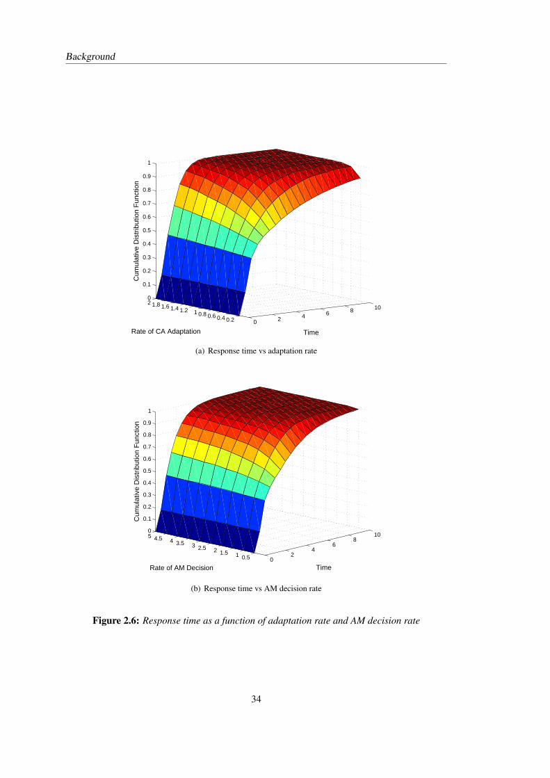
Background
0 2 4 6 8 10
0.20.40.60.811.21.41.61.820
0.1
0.2
0.3
0.4
0.5
0.6
0.7
0.8
0.9
1
TimeRate of CA Adaptation
Cum
ulat
ive
Dis
trib
utio
n F
unct
ion
(a) Response time vs adaptation rate
02
46
810
0.511.522.533.544.550
0.1
0.2
0.3
0.4
0.5
0.6
0.7
0.8
0.9
1
TimeRate of AM Decision
Cum
ulat
ive
Dis
trib
utio
n F
unct
ion
(b) Response time vs AM decision rate
Figure 2.6: Response time as a function of adaptation rate and AM decision rate
34
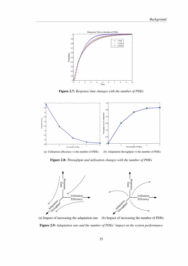
Background
0 1 2 3 4 5 6 7 8 9 100
0.1
0.2
0.3
0.4
0.5
0.6
0.7
0.8
0.9
1Response Time vs Number of PDEs
Time
Pro
babi
lity
1 PDE
2 PDEs
3 PDEs
Figure 2.7: Response time changes with the number of PDEs
1 2 3 4 50.25
0.3
0.35
0.4
0.45
0.5
0.55
0.6
0.65
0.7
The Number of PDEs
Pro
port
ion
of C
A1
(a) Utilisation efficiency vs the number of PDEs
1 2 3 4 50.2
0.25
0.3
0.35
0.4
0.45
0.5
The Number of PDEs
Thr
ough
put o
f CA
Ada
ptat
ion
(b) Adaptation throughput vs the number of PDEs
Figure 2.8: Throughput and utilisation changes with the number of PDEs
Response Tim
e
Utilisation Efficiency
Adapta
tion
Throug
hput
Response Tim
e
Utilisation Efficiency
Adapta
tion
Throug
hput
(a) Impact of increasing the adaptation rate (b) Impact of increasing the number of PDEs
Figure 2.9: Adaptation rate and the number of PDEs’ impact on the system performance
35
Background
appropriately dimension a system to achieve its potential.
As illustrated by Figure 2.9, as well as the reward equation, R =∑
s∈S ρ(s)π(s), the system
performance is affected by the activity rates and the populations of components (in the reward
equation, these two factors determine the steady-state probability distribution π). But we do
not know how these factors explicitly and analytically impact on the performance. As we will
see in Chapter 7, the performance is governed by a set of nonlinear algebra equations in the
sense of approximation. Based on those nonlinear equations, we clearly know how the system
will perform when the rates or populations change. Since these equations can be easily derived
according to the corresponding PEPA model, the performance optimisation based on them will
be much simpler and more convenient.
2.4.4 Enhancing PEPA to evaluate large scale content adaptation systems
The previous subsections have presented the performance analysis for the content adaptation
framework proposed by the Mobile VCE. Furthermore, for the architecture design of the com-
ponent adaptation manager, we have shown in [ADLM08] that the adaptation gateway of this
entity is a potential bottleneck for the system, suggesting that concurrent handling of adaptation
requests should be adopted. In the aforementioned papers [Dey00,CCC05a,CCC05b,CCL05],
some performance analyses, especially the distribution of the response time have also been
presented.
However, these analyses are based on small scale systems, i.e., not many users and servers
are taken into consideration. A realistic system may comprise a large number of users and
entities. Modelling systems at large scale can provide some insights about the system perfor-
mance which cannot be obtained via small scale modelling. For example, as we will see from
Figure 7.7(a) and Figure 7.7(b) in Chapter 7, the throughput of activities will remain flat after
some critical points in terms of the numbers of users, reflecting no improvement of performance
after the system resources are fully utilised. This important fact cannot be illustrated by results
such as those shown in Figure2.8 (b), which are based on small scale modelling.
Performance evaluation for large scale content adaptation systems has been considered in [DHL].
In this paper, the Monte Carlo simulation method is adopted to derive the response time from
the system model. But the computational complexity, mainly in terms of the convergence speed
of simulation, is very high and thus it is not possible to make real-time performance monitoring
36
Background
or prediction available.
In order to efficiently carry out performance evaluation as well as qualitative validation for large
scale content adaptation systems, we have to find appropriate approaches. In the following
chapters we will present our enhancement and investigations for PEPA. The new techniques
will be utilised to assess large scale content adaptation systems, which will be presented in
Chapter 7.
2.5 Related work
In the past fifteen years, many techniques dealing with the state-space explosion problem have
been developed for performance modelling paradigms including the stochastic process algebra
PEPA. This section presents a brief overview on these techniques, with a focus on PEPA.
2.5.1 Decomposition technique
For a Markov process with large state space, it is often not possible to get the exact solution or
the equilibrium distribution because there are not enough time and storage resources to generate
the states and the transition rates, or to solve the associated balanced equation. One approach
proposed to deal with this problem is that the solution of the single system can be formed
by a set of solutions which correspond to a set of subsystems. This approach is introduced
by Simon and Ando in [SA61] and called the decomposition / aggregation approach to the
solution of CTMC. A variety of decompositional techniques have been proposed to aid in
the solution of large Markov processes. According to the paper [Hil98] written by Hillston,
these decompositional techniques can be classed into two categories: product form solution
and aggregated decomposed solution. The following introduction to these techniques is mainly
based on the paper [Hil98].
2.5.1.1 Product form solutions
If a Markov process can be decomposed into subsystems which behave as if they are statisti-
cally independent, and the equilibrium distribution of this Markov process can be written as a
product of the equilibrium distributions of those subsystems, then this Markov process is said
to have product form solution or product form distribution. Clearly product form solutions are
37
Background
an efficient mechanism in deriving the performance from a Markovian model since there is no
need to generate the entire state space of the model.
Product form distributions have been widely used in the analysis of queueing networks [BCMP75]
and Petri nets. Based on earlier work on product form criteria for stochastic Petri nets [BS94,
HLT89, HT91], preliminary work on deriving product form criteria for stochastic process al-
gebras such as PEPA has been reported by Sereno in [Ser95]. In this paper, the method to
characterise the class of models which have a product form is based on the routing processes,
and relies on vector representations of the state and the action of a model. In this approach,
the routing process is a defined Markov chain in which the states correspond to the actions of
the PEPA model, and its balance equations correspond to the traffic equations of a queueing
network. As pointed out in [Ser95], if the state space of this process can be partitioned into
equivalence classes of enabling actions, then a product form solution exists.
A product form in the context of stochastic Petri nets, where the decomposition is carried out
over subnets, has been investigated by Lazar and Robertazzi in [LR91]. The results in [LR91]
are generalised by Boucherie in [Bou94] to characterise a class of Markov processes. The
processes belonging to this class can be formed as the product of a set of Markov processes
which compete over a set of resources. In [HT99], Hillston and Thomas characterise this class
of Markov processes in the PEPA language: these models consist of independent components,
which give rise to the constituent Markov processes of the underlying Markov processes, and
these components are connected indirectly through synchronisation with resource components.
In this paper, the cases in which these models exhibit a product form solution have been identi-
fied, so that the components of the model are solved in isolation, these partial solutions subse-
quently being combined to give a solution of the complete model.
A new derived combinator for PEPA has been presented and used to construct models which
have an insensitive structure by Clark and Hillston in the paper [CH02]. This structure is
characterised by an underlying CTMC that is insensitive, that is, its steady-state distribution
depends on the distribution of one or more of the random variables representing residence in
a state only through their mean. In this structure, a particular set of activities are therefore
not necessarily assumed to be exponentially distributed. The identified model structure has
a product form solution, which does not match the previous criteria for the currently known
stochastic process algebra product form classes [CH02].
38
Background
Not all PEPA models have product form solution, because the necessary structural conditions
are stringent. Some classes of models have been transformed into new models which are prod-
uct form, based on modifications of the PEPA expressions representing them [TH00].
Product-form solutions in Markovian process algebras such as PEPA can be constructed using
the Reversed Compound Agent Theorem (RCAT), as shown by Harrison in [Har03]. The RCAT
is a compositional result used to determine the reversed processes. From a reversed process,
a product form solution for the joint state probabilities follows directly. Therefore, the RCAT
provides an alternative methodology for finding product-form solutions in PEPA. The RCAT
has been generalised by the same author in two ways in [Har04]. The first generalisation was,
by relaxing two conditions of the original RCAT, to yield a more general result that applies to
a wider class of concurrent systems. Another generalisation was “obtained and used to derive
the equilibrium state probabilities in a similar staged queue with processor sharing queueing
discipline”, which lead to a non-product form solution for a class of queueing networks with
global state-dependence. Some further investigation and application of non-product forms can
be found in [Har06] and [Tho06]. More recently, a type of product-form was obtained by
Fourneau et al. in [FPS07] for a pair of CTMCs, expressed as stochastic automata networks,
which did not have synchronised transitions but in which the rate of a transition in either chain
depended on the current state of the other chain. The conditions derived in [FPS07] for a
product-form to exist at equilibrium, have been obtained alternatively in [Har09] using a special
case of RCAT.
2.5.1.2 Aggregated decomposed solutions
In addition to the product form solution, there is another decomposed solution technique that
is suggested by the stochastic process algebra model structure, called the aggregated decom-
posed solution. This approach involves a stochastic representation of the interactions between
components, and the solution of the single model is obtained by a set of solutions of submodels
using an aggregated version of the original model.
Work on time scale decomposition in PEPA, based on Courtois’s near complete decompos-
ability [Cou77], has been presented by Hillston and Mertsiotakis in [HM95]. Time scale de-
composition is a popular aggregated decomposition technique, which decomposes a CTMC
so that short term equilibrium is reached within single partitions, and partition changes occur
only rarely as the process approaches its long term equilibrium [SA61, HM95]. The work re-
39
Background
ported in [HM95] is inspired by related work on time scale decomposition of stochastic Petri
nets [ARI89, BT93], and relies on a classification of all actions relative to some threshold rate.
Later work to tackle the problem of hybrid components which enable both fast and slow actions
is presented in [Mer98,Mer97]. The slow behaviour of the hybrid was extracted into a separate
shadow component, making the original component passive with respect to these actions.
Decision free processes is another approach to the decomposition of a class of stochastic pro-
cess algebra models. In this approach, the model is partitioned into components, and they are
then recombined so that one component is fully represented while the other is reduced to a
minimal form, usually consisting of a single transition. For the work about the application of
this approach to throughput approximation, see [Mer98, MS96, MS97].
There are several other kinds of decomposition techniques including the technique based on the
notion of near-independence and the technique of decomposition via synchronisation points.
Components are considered by Ciardo and Trivedi to be near-independent if they operate in
parallel and rarely interact [CT91]. Following the basic idea that near-independent components
can be solved independently in conjunction with a graph model which represents the dependen-
cies, a near-independence based decomposition technique was proposed for stochastic reward
nets [CT91]. It has been suggested by Bohnenkamp and Haverkort in [BH97] that this tech-
nique could be adapted for stochastic process algebra models. In the proposed approach the
dependence between parallel components was recognised as the actions on which they coop-
erate. In [BH99] Bohnenkamp and Haverkort considered, within a stochastic process algebra
framework, a class of models in which there was a fixed number of sequential processes run-
ning in parallel and synchronising on the same global set of actions. Within this class of models
their solution technique is exact with respect to throughput and local steady-state probabilities.
2.5.2 Tensor representation technique
Another technique which has been taken to exploit the model compositionality is the use of
Kronecker algebra. Kronecker algebra representations were first developed by Plateau in the
context of stochastic automata networks [Pla84, Pla85], to analytically represent the genera-
tor matrix of the Markov process underlying a stochastic automata network model. This tech-
nique can relieve the state-space explosion problem arising in the numerical solution of Markov
chains since the solution can be achieved via this tensor expression of submatrices and the com-
plete matrix does not need to be generated. More recently, Kronecker-based solution techniques
40
Background
have been developed for various Petri net based formalisms, see [Don94,Kem96,CM99,DK00].
Analogous to the representation of a stochastic automata network, it has been demonstrated
by Hillston and Kloul in [HK01] that PEPA models can be represented analytically using Kro-
necker algebra and solved without constructing the complete generator matrix. Furthermore,
this Kronecker representation has been combined with the aggregation technique to deal with
larger models [HK07]. However, as pointed out in [HK07], these techniques “can be viewed as
shifting the problem rather than avoiding it, in the sense that there are still fundamental limits
on the size of model which can be analysed”.
In addition, this tensor representation technique has also been applied to an extension of PEPA
(see [ER00]) and other stochastic process algebras such as Markovian process algebra [Buc94]
and TIPP [RS94].
2.5.3 Abstraction and stochastic bound techniques
Smith discussed another way to analyse large scale PEPA models in his series of papers [Smi09a,
Smi09b,Smi09c], i.e. using abstraction — constructing a smaller model that bounds the proper-
ties of the original. Abstract Markov chains [FLW06,KKLW07] and stochastic bounds [FLQ04,
SD83] are two techniques used for producing bounded abstractions of a CTMC: the former can
be used to bound transient properties, and the latter for various monotone properties such as
the steady-state distribution [Smi09a]. These two techniques are originally specified and used
in the context of Markov chains, but have been extended, based on a Kronecker representation
for the generator matrix of a PEPA model [HK01], so that they can be applied compositionally
to PEPA models [Smi09b]. An algorithm for constructing a compositional upper bound of a
PEPA component has also been presented in [Smi09b].
2.5.4 Fluid approximation technique
The techniques reported above are based on the discrete state space. However, as the size of
the state space is extremely large, these techniques are not always strong enough to handle the
state-space explosion problem. To avoid this problem Hillston proposed a radically different
approach in [Hil05a] from the following two perspectives: choosing a more abstract state rep-
resentation in terms of state variables, quantifying the types of behaviour evident in the model;
and assuming that these state variables are subject to continuous rather than discrete change.
41
Background
This approach results in a set of ODEs, leading to the evaluation of transient, and in the limit,
steady state measures.
An interpretation as well as a justification of this approximation approach has been demon-
strated by Hayden in his dissertation [Hay07a]. In [Hay07a, HB08], generation of similar sys-
tems of coupled ODEs for higher-order moments such as variance has been addressed. Ad-
ditionally, the dissertation [Hay07a] discusses how to derive stochastic differential equations
from PEPA models.
More recently, some extensions of the previous mapping from PEPA to ODEs have been pre-
sented by Bradley et al. in [BGH07]. In particular, passive rates are introduced into the fluid
approximation. In the recent paper [HB10], different existing styles of passive cooperation
in fluid models are compared and intensively discussed. Moreover, a new passive fluid se-
mantics for passive cooperation, which can be viewed as approximating the first moments of
the component counting processes, has been provided, with a theoretical justification. The
paper [BHM+09] considers the application of this fluid approximation approach with modi-
fications in the context of epidemiology. In this paper, the notions of side and self-loops are
added to the activity matrix, and the rates are calculated differently, for the purpose of deriving
from PEPA models the most commonly used ODEs in the context of epidemiology. In [Tri09]
by Tribastone, a new operational semantics is proposed to give a compact symbolic representa-
tion of PEPA models. This semantics extends the application scope of the fluid approximation
of PEPA by incorporating all the operators of the language and removing earlier assumptions
on the syntactical structure of the models amenable to this analysis.
The fluid approximation approach has also been applied to timed Petri nets to deal with the
state-space explosion problem [SR05, MRS06]. The comparison between the fluid approx-
imation of PEPA models and timed continuous Petri nets has been demonstrated by Galpin
in [Gal08]. This paper has established links between two continuous approaches to modelling
the performance of systems. In the paper, a translation from PEPA models to continuous Petri
nets and vice versa has been presented. In addition, it has been shown that the continuous ap-
proximation using PEPA has infinite server semantics. The fluid approximation approach has
also been used by Thomas to derive asymptotic solutions for a class of closed queueing net-
works [Tho09]. In this paper, an analytical solution to a class of models, specified using PEPA,
is derived through the ODE approach. It is shown that “this solution is identical to that used for
many years as an asymptotic solution to the mean value analysis of closed queueing networks”.
42
Background
Moreover, the relationship between the fluid approximation and the underlying CTMCs for a
special PEPA model has been revealed by Geisweiller et al. in [GHS08]: the ODEs derived
from the PEPA description are the limits of the sequence of underlying CTMCs. It has been
shown in [Gil05] by Gilmore that for some special examples the equilibrium points of the ODEs
derived from PEPA models coincide the steady-state probability distributions of the CTMCs
underlying the nonsynchronised PEPA models.
In addition, there are several papers which discuss how to derive response time from the fluid
approximation of PEPA models. In [BHKS08], by constructing an absorption operator for the
PEPA language, Bradley et al. allow general PEPA models to be analysed for fluid-generated
response times. Clark et al. demonstrate in [CDGH08] how to derive expected passage response
times using Little’s law based on averaged populations of entities in an equilibrium state. This
technique has been generalised into one for obtaining a full response-time profile computing
the probability of a component observing the completion of a response at a given time after
the initiation of the request, see [Cla09]. Moreover, an error in the passage specification in the
approach taken in [BHKS08] has been uncovered and rectified in [Cla09] by Clark.
The ODE method associated with the PEPA language has demonstrated successful application
in the performance analysis of large scale systems. In Harrison and Massink’s paper [HM09],
quantitative models of a class of ubiquitous systems, including a guidance system to assist
out-patients in a hospital, are considered and analysed using PEPA and the associated ODE
approximation approach. The analyses provide insight into the impact of a ubiquitous system
design on the congestion experienced by users in different traffic situations. This paper shows
that “the ODE approach is an attractive alternative to simulation to explore the effect on visitor
flows for different design options during early design phases”.
Zhao and Thomas’s paper [ZT08] considers a PEPA model of a key distribution centre. By
combining successive internal actions into a single action with a modified rate, the system be-
haviour is approximated by a simpler model, a queueing network model which gives explicit
performance measures. The fluid approximation was derived from the simplified models and
compared to the queueing approximation in [TZ08,ZT09]. A limitation of the fluid approxima-
tion approach has been pointed out in [ZT09]: not all desired metrics can be obtained.
The work on the fluid approximation of PEPA reported above mainly deals with some exten-
sions to make this approach more applicable or demonstrates its applications in some specific
43
Background
areas. However, there are not many discussions on the fundamental problems, such as the exis-
tence, uniqueness, boundedness and nonnegativeness of the solution, as well as the its asymp-
totic behaviour as time tends to infinity, and the relationship between the derived ODEs and the
underlying CTMCs for general PEPA models. As for applications, the basic problem of what
kind of performance metrics can and cannot be derived through this approach, has also not
been discussed generally and in detail. This thesis will focus on these topics and give answers
to these problems.
2.6 Summary
In this chapter, we have introduced the content adaptation framework proposed by the Mobile
VCE as well as the PEPA language. For small scale content adaptation systems based on
this framework, the PEPA modelling and evaluation have been presented. Some parts of this
work have been published as a joint work in the Journal of Wireless Personal Communications,
see [DHL09]. This chapter has also presented a review of the related work on dealing with
the state-space explosion problem in the current performance modelling paradigms, with an
emphasis on the PEPA language.
44
Chapter 3
New Representation for PEPA: fromSyntactical to Numerical
3.1 Introduction
This chapter defines a numerical presentation scheme for PEPA, for the purpose of applying
powerful mathematical tools and methods for both qualitative and quantitative analysis of large
scale PEPA models with repeated components. In this presentation scheme, a state of a system
is represented by a numerical vector, with each entry being a non-negative integer recording
the population of the components in the corresponding local derivative. Any transition between
states is indicated by a labelled activity, or equivalently, a transition vector. All the transition
vectors form an activity matrix, which captures the structural information of the given model.
The average duration of labelled activities or transitions are specified by transition rate functions
that are defined to capture the timing information of the system.
The fact that the structural and timing information is captured means that the representation can
provide a platform to directly employ mathematical methods such as linear programming and
differential equations to analyse a PEPA model. This chapter presents a technical preparation
including the definitions and some fundamental investigations of the new representation, for
the further study of PEPA appearing in the following chapters.
The remainder of this chapter is structured as follows. Section 3.2 gives the definition of the
numerical vector form which is used to represent the states of PEPA models. The efficiency of
this form is demonstrated. Labelled activities and activity matrices are defined in Section 3.3
while Section 3.4 defines transition rate functions. The consistency between these definitions
and PEPA language is formulated as propositions. An algorithm is given for automatically
deriving the labelled activities, activity matrix and transition rate functions from any PEPA
model. Section 3.5 presents an initial discussion of how to utilise some efficient approaches to
investigate PEPA models. Finally, a summary is presented in Section 3.6.
45
New Representation for PEPA: from Syntactical to Numerical
3.2 Numerical Vector Form
The numerical vector form, proposed by Hillston in [Hil96] as a model aggregation technique
to represent the states of PEPA models with repeated components, can efficiently decrease
the size the underlying state space from exponential to at most polynomial in the number of
components. This section discusses the definition and efficiency of the numerical vector form.
3.2.1 State-space explosion problem: an illustration by a tiny example
Let us first consider the following tiny example. A User-Provider system is composed of
two types of entities: User and Provider. The communication between them is through a
shared activity task1. After task1 is fired, User1 becomes User2 while Provider1 becomes
Provider2 simultaneously. User2 can fire task2 and then go back to User1. Provider2 will
become Provider1 when reset is fired. The PEPA model for this User-Provider system is
illustrated below:
Model 1. PEPA Model of User-Provider System
PEPA Definition for User:
User1def=(task1, a).User2
User2def=(task2, b).User1
PEPA Definition for Provider:
Provider1def=(task1, a).P rovider2
Provider2def=(reset, d).P rovider1
System Equation:
User1|| · · · ||User1︸ ︷︷ ︸M copies
BC{task1}
Provider1|| · · · ||Provider1︸ ︷︷ ︸N copies
The system equation in a PEPA model specifies how many copies of each entity are presented
in the system, and how the components interact, by forcing cooperation on some of the activity
types. In Model 1, the exact numbers of independent copies of the User and Provider, i.e.
M and N respectively, are both considered as variables. According to the semantics of PEPA
46
New Representation for PEPA: from Syntactical to Numerical
originally defined in [Hil96], the size of the state space of the CTMC underlying Model 1 is
2M+N . That is, the size of the state space increases exponentially with the numbers of the
users and providers in the system. Consequently, the dimension of the infinitesimal generator
of the CTMC is 2M+N × 2M+N . The computational complexity of solving the global balance
equation to get the steady-state probability distribution and thus derive the system performance,
is therefore exponentially increasing with the numbers of the components. When M and/or N
are large, the calculation of the stationary probability distribution will be infeasible due to
limited resources of memory and time. The problem encountered here is the so-called state-
space explosion problem.
Not only quantitative but also qualitative analysis suffers from the state-space explosion prob-
lem. For example, it is impossible to explore the entire state space with limited resources to
check whether there is a deadlock. In fact, even the derivation and storage of the state space
can become a problem since it is very large.
Fortunately, a model aggregation technique introduced by Gilmore et al. in [GHR01] and by
Hillston in [Hil05a] can help to relieve the state-space explosion problem.
3.2.2 Definition of numerical vector form
We have introduced in 2.3.3 that in PEPA the state representation is in fact a labelled multi-
transition system. This is also termed the derivation graph. The usual state representation in
PEPA models is in terms of the syntactic forms of the model expression. Thus, as pointed
out in [Hil05a], each node in the derivation graph is a distinct syntactic form and each arc
represents a possible activity causing the state change. Clearly, if the action types are ignored,
the derivation graph can be considered to be the state transition diagram of a CTMC.
When a large number of repeated components are involved in a system, the state space of the
CTMC can be large, as Model 1 shows. This is mainly because each copy of the same type
of component is considered to be distinct, resulting in distinct Markovian states. The multiple
states within the model that exhibit the same behaviour can be aggregated to reduce the size of
the state space as shown by Gilmore et al. [GHR01] using the technique based on a vector form.
The derivation graph is therefore constructed in terms of equivalence classes of syntactic terms.
“At the heart of this technique is the use of a canonical state vector to capture the syntactic form
of a model expression”, as indicated in [Hil05a], “if two states have the same canonical state
47
New Representation for PEPA: from Syntactical to Numerical
vector they are equivalent and need not be distinguished in the aggregated derivation graph”.
Rather than the canonical representation style, an alternative numerical vector form was pro-
posed by Hillston in [Hil05a] for capturing the state information of models with repeated com-
ponents. In the numerical vector form, there is one entry for each local derivative of each type
of component in the model. The entries in the vector are the number of components currently
exhibiting this local derivative, no longer syntactic terms representing the local derivative of the
sequential component. Following [Hil05a], hereafter the term local derivative refers to the local
state of a single sequential component, whereas derivative is used for a global state represented
in its syntactic form. The definition of numerical vector form is given below.
Definition 3.2.1. (Numerical Vector Form [Hil05a]). For an arbitrary PEPA model M with
n component types Ci, i = 1, 2, · · · , n, each with di distinct local derivatives, the numerical
vector form of M, m(M), is a vector with d =∑n
i=1 di entries. The entry m[Cij ] records
how many instances of the jth local derivative of component type Ci are exhibited in the current
state.
According to Definition 3.2.1, the discrimination between any two system states is characterised
by the two system vectors. That is, if the two vectors are different then the two states are
considered different, otherwise they are the same.
For a sequential component Ci with the local derivatives Ci1 , Ci2 , · · · , Cidi, define
m(Ci) :=(m[Ci1 ],m[Ci2 ], · · · ,m[Cidi
])T
,
where m is the system vector. So m(Ci) is a subvector of m, which can be considered the
restriction of the system vector in the context of the sequential component Ci. For convenience,
m(Ci) is called the state vector of the sequential component Ci or the state vector of component
type Ci, or just Ci’s vector for short.
Remark 3.2.1. Obviously m(Cij ) ≥ 0 for each Cij . At any time, each sequential component
stays in one and only one local derivative. So the sum of m(Ci), i.e.∑di
j=1 m[Cij ], specifies
the population of Ci in the system. In other words, if there are Mi copies of the sequential
component Ci in the system, then∑di
j=1 m[Cij ] = Mi for any system state.
The entries in the system vector or a sequential component’s vector are no longer syntactic
terms representing the local derivative, but the number of components currently exhibiting this
48
New Representation for PEPA: from Syntactical to Numerical
local derivative. This model-aggregation technique can significantly reduce the size of the state
space, i.e. the number of the system states.
3.2.3 Efficiency of numerical vector form
By adopting the new representation technique, the number of the states of the system can be re-
duced to only increase (at most) polynomially with the number of instances of the components.
This fact is stated in the following Proposition 3.2.1. Before turning to this conclusion a lemma
is introduced, which will be used in the proof of the proposition.
Lemma 3.2.1.
#
(a1, a2, · · · , ad) :d∑
j=1
ai = m,aj ∈ Z+(j = 1, 2, · · · , d)
=
m + d− 1
d− 1
.
where #A is defined as the cardinality of the set A, i.e. the number of elements of A; Z+ is the
set of nonnegative integers. This a well-known combinatorial formula. Readers are referred to
Theorem 3.5.1 in [Bru98] for reference. Lemma 3.2.1 specifies how many solutions satisfy the
condition a1, a2, · · · , ad ≥ 0, aj ∈ Z (j = 1, 2, · · · , d),∑dj=1 aj = m.
Apply Lemma 3.2.1 to the vector of Ci defined in the last subsection,
m(Ci) =(m[Ci1 ],m[Ci2 ], · · · ,m[Cidi
])T
,
where, by Remark 3.2.1, provided there are Mi copies of Ci in the system, m(Ci) satisfies m[Ci1 ],m[Ci2 ], · · · ,m[Cidi] ∈ Z+,∑d
j=1 m[Cij ] = Mi.(3.1)
Then there are at most
Mi + di − 1
di − 1
solutions, i.e.
Mi + di − 1
di − 1
states in terms of
Ci in the system. The phrase “at most” used here is to reflect that
Mi + di − 1
di − 1
is an upper
bound of the exact number of the states in terms of Ci, since the possible synchronisations in
49
New Representation for PEPA: from Syntactical to Numerical
the PEPA model have not been taken into account in the restrictions (3.1) and thus the current
restrictions may allow extra freedom for the solutions. This argument leads to the following
Proposition 3.2.1. Consider a system comprising n types of component, namely C1, C2, · · · , Cn,
with Mi copies of the component of type Ci in the system, where Ci has di local derivatives,
for i = 1, 2, · · · , n. Then the size of the state space of the system is at most
n∏i=1
Mi + di − 1
di − 1
≤n∏
i=1
(mi + di − 1)di−1 .
Proof. For each component type Ci, there are at most
Mi + di − 1
di − 1
solutions for the
system vector. So the total number of states of the system is at most∏n
i=1
Mi + di − 1
di − 1
.
Notice Mi + di − 1
di − 1
=(Mi + di − 1)(Mi + di − 2) · · · (Mi + 1)
(di − 1)!≤ (Mi + di − 1)di−1 ,
son∏
i=1
Mi + di − 1
di − 1
≤n∏
i=1
(Mi + di − 1)di−1 .
This completes the proof.
Proposition 3.2.1 gives an upper bound, e.g.∏n
i=1 (Mi + di − 1)di−1, for the size of the state
space of the given system. In this term, n and di are fixed in the PEPA definition for the system,
while Mi can be considered as variables which refer to the numbers of the repeated components.
This bound guarantees that the size of the state space increases at most polynomially with the
number of instances of the components. Since the state space of a model is the foundation
for both qualitative and quantitative analysis, the size of the state space mainly determines
the computational complexity of the state-space-based algorithms for analysing the system.
For example, since the current deadlock-checking algorithm needs to explore the entire space
to find whether there is a deadlock, so the efficiency, of course, depends on the size of the
state space. As for quantitative analysis, the performance measures such as throughput and
utilisation, obviously suffer the size of the state space because they derive from the equilibrium
probabilities distributed on each state in the space. Compared to the exponential increase of
50
New Representation for PEPA: from Syntactical to Numerical
state space size, the benefit brought by the new representation is very significant. An illustration
of the state space represented in the numerical vector form for the previous example, is given
in the next subsection.
3.2.4 Model 1 continued
This subsection presents the state space for Model 1 in Section 3.2.1:
User1def=(task1, a).User2
User2def=(task2, b).User1
Provider1def=(task1, a).P rovider2
Provider2def=(reset, d).P rovider1
User1[M ] BC{task1}
Provider1[N ].
In the model, there are two component types, User and Provider; each has two local deriva-
tives, User1, User2 and Provider1, Provider2 respectively. According to Definition 3.2.1,
the system vector m has four entries representing the instances of components in the total four
local derivatives, that is
m = (m[User1],m[User2],m[Provider1],m[Provider2])T .
Let M = N = 2, then the system equation of Model 1 determines the starting state:
m = (M, 0, N, 0)T = (2, 0, 2, 0)T := s1.
After firing the synchronised activity task1, then one instance of User1 and one copy of
Provider1 become User2 and Provider2 simultaneously and respectively. Then the system
vector becomes s2 = (1, 1, 1, 1)T , reflecting each local derivative being occupied by one com-
ponent. By enabling activities or transitions, all reachable system states can be manifested as
follows:
s1 = (2, 0, 2, 0)T , s2 = (1, 1, 1, 1)T , s3 = (1, 1, 2, 0)T ,
s4 = (1, 1, 0, 2)T , s5 = (0, 2, 1, 1)T , s6 = (2, 0, 1, 1)T ,
s7 = (0, 2, 0, 2)T , s8 = (0, 2, 2, 0)T , s9 = (2, 0, 0, 2)T .
(3.2)
51
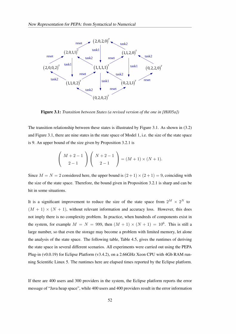
New Representation for PEPA: from Syntactical to Numerical
( )2,0,2,0 T
( )1,1,2,0 T
( )2,0,0,2 T
( )2,0,1,1 T
( )0,2,0,2 T
( )1,1,1,1 T
( )0,2,1,1 T( )1,1,0,2 T
( )0,2,2,0 T
task1
task1
task2
task2
reset
reset task2 reset
task1 task1
resettask2
task2
reset task2
reset
Figure 3.1: Transition between States (a revised version of the one in [Hil05a])
The transition relationship between these states is illustrated by Figure 3.1. As shown in (3.2)
and Figure 3.1, there are nine states in the state space of Model 1, i.e. the size of the state space
is 9. An upper bound of the size given by Proposition 3.2.1 is M + 2− 1
2− 1
N + 2− 1
2− 1
= (M + 1)× (N + 1).
Since M = N = 2 considered here, the upper bound is (2 + 1)× (2 + 1) = 9, coinciding with
the size of the state space. Therefore, the bound given in Proposition 3.2.1 is sharp and can be
hit in some situations.
It is a significant improvement to reduce the size of the state space from 2M × 2N to
(M + 1) × (N + 1), without relevant information and accuracy loss. However, this does
not imply there is no complexity problem. In practice, when hundreds of components exist in
the system, for example M = N = 999, then (M + 1) × (N + 1) = 106. This is still a
large number, so that even the storage may become a problem with limited memory, let alone
the analysis of the state space. The following table, Table 4.5, gives the runtimes of deriving
the state space in several different scenarios. All experiments were carried out using the PEPA
Plug-in (v0.0.19) for Eclipse Platform (v3.4.2), on a 2.66GHz Xeon CPU with 4Gb RAM run-
ning Scientific Linux 5. The runtimes here are elapsed times reported by the Eclipse platform.
If there are 400 users and 300 providers in the system, the Eclipse platform reports the error
message of “Java heap space”, while 400 users and 400 providers result in the error information
52
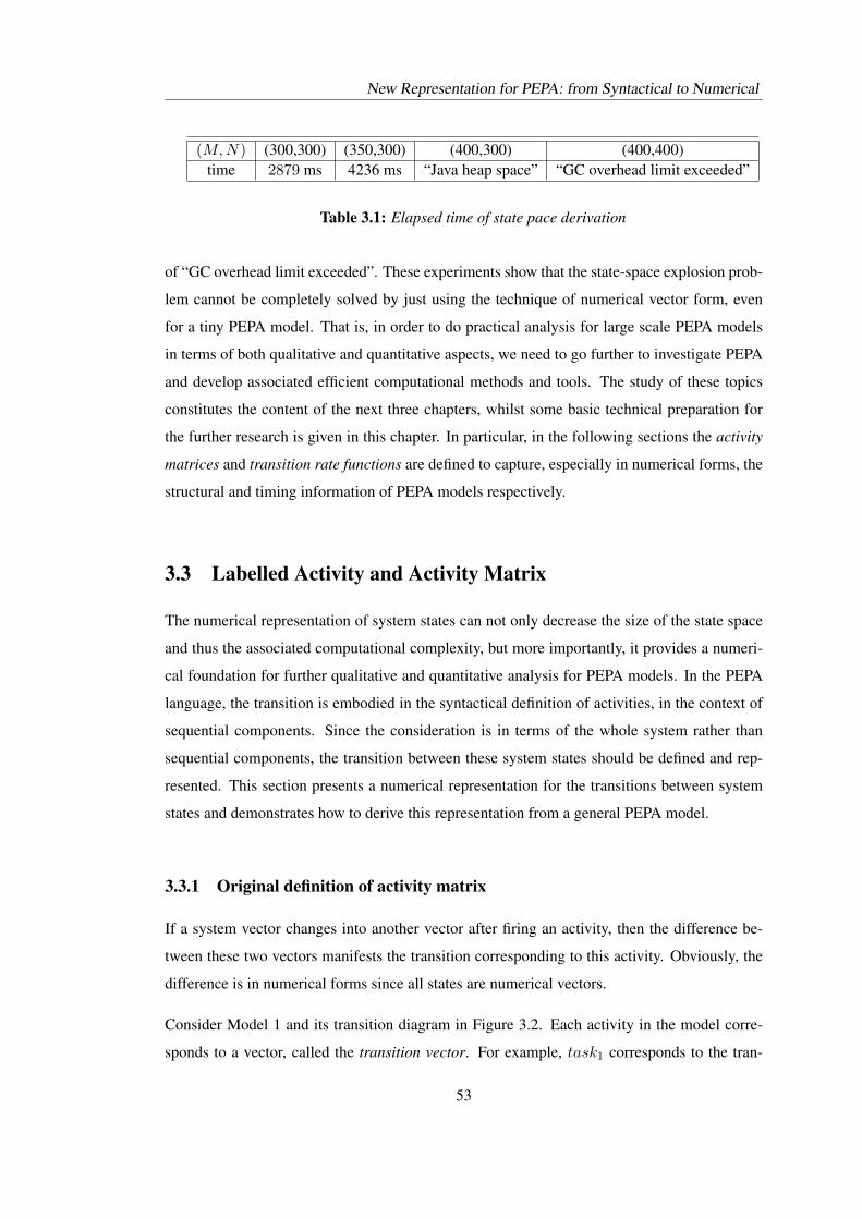
New Representation for PEPA: from Syntactical to Numerical
(M,N) (300,300) (350,300) (400,300) (400,400)time 2879 ms 4236 ms “Java heap space” “GC overhead limit exceeded”
Table 3.1: Elapsed time of state pace derivation
of “GC overhead limit exceeded”. These experiments show that the state-space explosion prob-
lem cannot be completely solved by just using the technique of numerical vector form, even
for a tiny PEPA model. That is, in order to do practical analysis for large scale PEPA models
in terms of both qualitative and quantitative aspects, we need to go further to investigate PEPA
and develop associated efficient computational methods and tools. The study of these topics
constitutes the content of the next three chapters, whilst some basic technical preparation for
the further research is given in this chapter. In particular, in the following sections the activity
matrices and transition rate functions are defined to capture, especially in numerical forms, the
structural and timing information of PEPA models respectively.
3.3 Labelled Activity and Activity Matrix
The numerical representation of system states can not only decrease the size of the state space
and thus the associated computational complexity, but more importantly, it provides a numeri-
cal foundation for further qualitative and quantitative analysis for PEPA models. In the PEPA
language, the transition is embodied in the syntactical definition of activities, in the context of
sequential components. Since the consideration is in terms of the whole system rather than
sequential components, the transition between these system states should be defined and rep-
resented. This section presents a numerical representation for the transitions between system
states and demonstrates how to derive this representation from a general PEPA model.
3.3.1 Original definition of activity matrix
If a system vector changes into another vector after firing an activity, then the difference be-
tween these two vectors manifests the transition corresponding to this activity. Obviously, the
difference is in numerical forms since all states are numerical vectors.
Consider Model 1 and its transition diagram in Figure 3.2. Each activity in the model corre-
sponds to a vector, called the transition vector. For example, task1 corresponds to the tran-
53
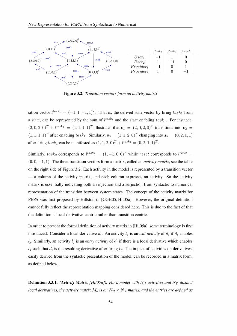
New Representation for PEPA: from Syntactical to Numerical
( )2,0,2,0 T
( )1,1,2,0 T
( )2,0,0,2 T
( )2,0,1,1 T
( )0,2,0,2 T
( )1,1,1,1 T
( )0,2,1,1 T( )1,1,0,2 T
( )0,2,2,0 T
task1
task1
task2
task2
reset
reset task2 reset
task1 task1
resettask2
task2
reset task2
reset
ltask1 ltask2 lreset
User1 −1 1 0User2 1 −1 0
Provider1 −1 0 1Provider2 1 0 −1
Figure 3.2: Transition vectors form an activity matrix
sition vector ltask1 = (−1, 1,−1, 1)T . That is, the derived state vector by firing task1 from
a state, can be represented by the sum of ltask1 and the state enabling task1. For instance,
(2, 0, 2, 0)T + ltask1 = (1, 1, 1, 1)T illustrates that s1 = (2, 0, 2, 0)T transitions into s2 =
(1, 1, 1, 1)T after enabling task1. Similarly, s3 = (1, 1, 2, 0)T changing into s5 = (0, 2, 1, 1)
after firing task1 can be manifested as (1, 1, 2, 0)T + ltask1 = (0, 2, 1, 1)T .
Similarly, task2 corresponds to ltask2 = (1,−1, 0, 0)T while reset corresponds to lreset =
(0, 0,−1, 1). The three transition vectors form a matrix, called an activity matrix, see the table
on the right side of Figure 3.2. Each activity in the model is represented by a transition vector
— a column of the activity matrix, and each column expresses an activity. So the activity
matrix is essentially indicating both an injection and a surjection from syntactic to numerical
representation of the transition between system states. The concept of the activity matrix for
PEPA was first proposed by Hillston in [CGH05, Hil05a]. However, the original definition
cannot fully reflect the representation mapping considered here. This is due to the fact of that
the definition is local-derivative-centric rather than transition centric.
In order to present the formal definition of activity matrix in [Hil05a], some terminology is first
introduced. Consider a local derivative di. An activity lj is an exit activity of di if di enables
lj . Similarly, an activity lj is an entry activity of di if there is a local derivative which enables
lj such that di is the resulting derivative after firing lj . The impact of activities on derivatives,
easily derived from the syntactic presentation of the model, can be recorded in a matrix form,
as defined below.
Definition 3.3.1. (Activity Matrix [Hil05a]). For a model with NA activities and ND distinct
local derivatives, the activity matrix Ma is an ND ×NA matrix, and the entries are defined as
54
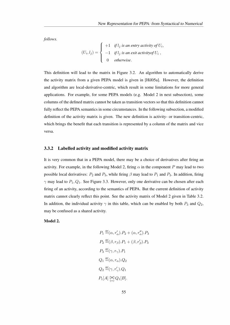
New Representation for PEPA: from Syntactical to Numerical
follows.
(Ui, lj) =
+1 if lj is an entry activity of Ui,
−1 if lj is an exit activityof Ui ,
0 otherwise.
This definition will lead to the matrix in Figure 3.2. An algorithm to automatically derive
the activity matrix from a given PEPA model is given in [Hil05a]. However, the definition
and algorithm are local-derivative-centric, which result in some limitations for more general
applications. For example, for some PEPA models (e.g. Model 2 in next subsection), some
columns of the defined matrix cannot be taken as transition vectors so that this definition cannot
fully reflect the PEPA semantics in some circumstances. In the following subsection, a modified
definition of the activity matrix is given. The new definition is activity- or transition-centric,
which brings the benefit that each transition is represented by a column of the matrix and vice
versa.
3.3.2 Labelled activity and modified activity matrix
It is very common that in a PEPA model, there may be a choice of derivatives after firing an
activity. For example, in the following Model 2, firing α in the component P may lead to two
possible local derivatives: P2 and P3, while firing β may lead to P1 and P3. In addition, firing
γ may lead to P1, Q1. See Figure 3.3. However, only one derivative can be chosen after each
firing of an activity, according to the semantics of PEPA. But the current definition of activity
matrix cannot clearly reflect this point. See the activity matrix of Model 2 given in Table 3.2.
In addition, the individual activity γ in this table, which can be enabled by both P3 and Q2,
may be confused as a shared activity.
Model 2.
P1def=(α, r′α).P2 + (α, r′′α).P3
P2def=(β, rβ).P1 + (β, r′β).P3
P3def=(γ, rγ).P1
Q1def=(α, rα).Q2
Q2def=(γ, r′γ).Q1
P1[A] BC{α}
Q1[B].
55
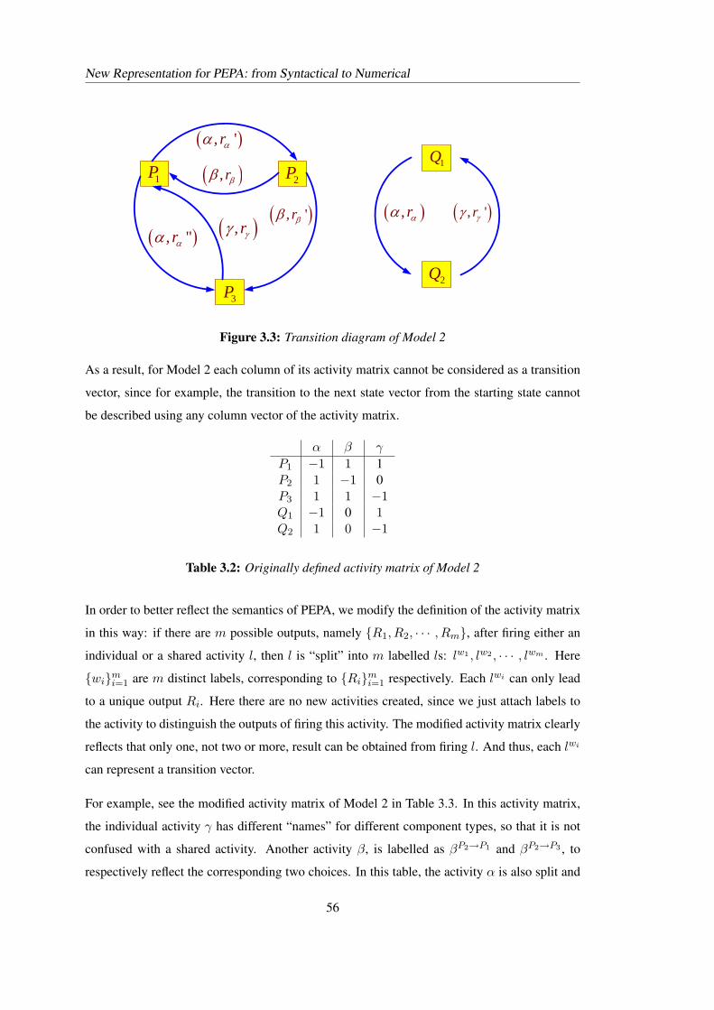
New Representation for PEPA: from Syntactical to Numerical
( ), rαα
1Q
2Q
1P 2P
3P
( ), 'rγγ
( ), 'rαα
( ), "rαα ( ), rγγ
( ), rββ
( ), 'rββ
Figure 3.3: Transition diagram of Model 2
As a result, for Model 2 each column of its activity matrix cannot be considered as a transition
vector, since for example, the transition to the next state vector from the starting state cannot
be described using any column vector of the activity matrix.
α β γ
P1 −1 1 1P2 1 −1 0P3 1 1 −1Q1 −1 0 1Q2 1 0 −1
Table 3.2: Originally defined activity matrix of Model 2
In order to better reflect the semantics of PEPA, we modify the definition of the activity matrix
in this way: if there are m possible outputs, namely {R1, R2, · · · , Rm}, after firing either an
individual or a shared activity l, then l is “split” into m labelled ls: lw1 , lw2 , · · · , lwm . Here
{wi}mi=1 are m distinct labels, corresponding to {Ri}m
i=1 respectively. Each lwi can only lead
to a unique output Ri. Here there are no new activities created, since we just attach labels to
the activity to distinguish the outputs of firing this activity. The modified activity matrix clearly
reflects that only one, not two or more, result can be obtained from firing l. And thus, each lwi
can represent a transition vector.
For example, see the modified activity matrix of Model 2 in Table 3.3. In this activity matrix,
the individual activity γ has different “names” for different component types, so that it is not
confused with a shared activity. Another activity β, is labelled as βP2→P1 and βP2→P3 , to
respectively reflect the corresponding two choices. In this table, the activity α is also split and
56
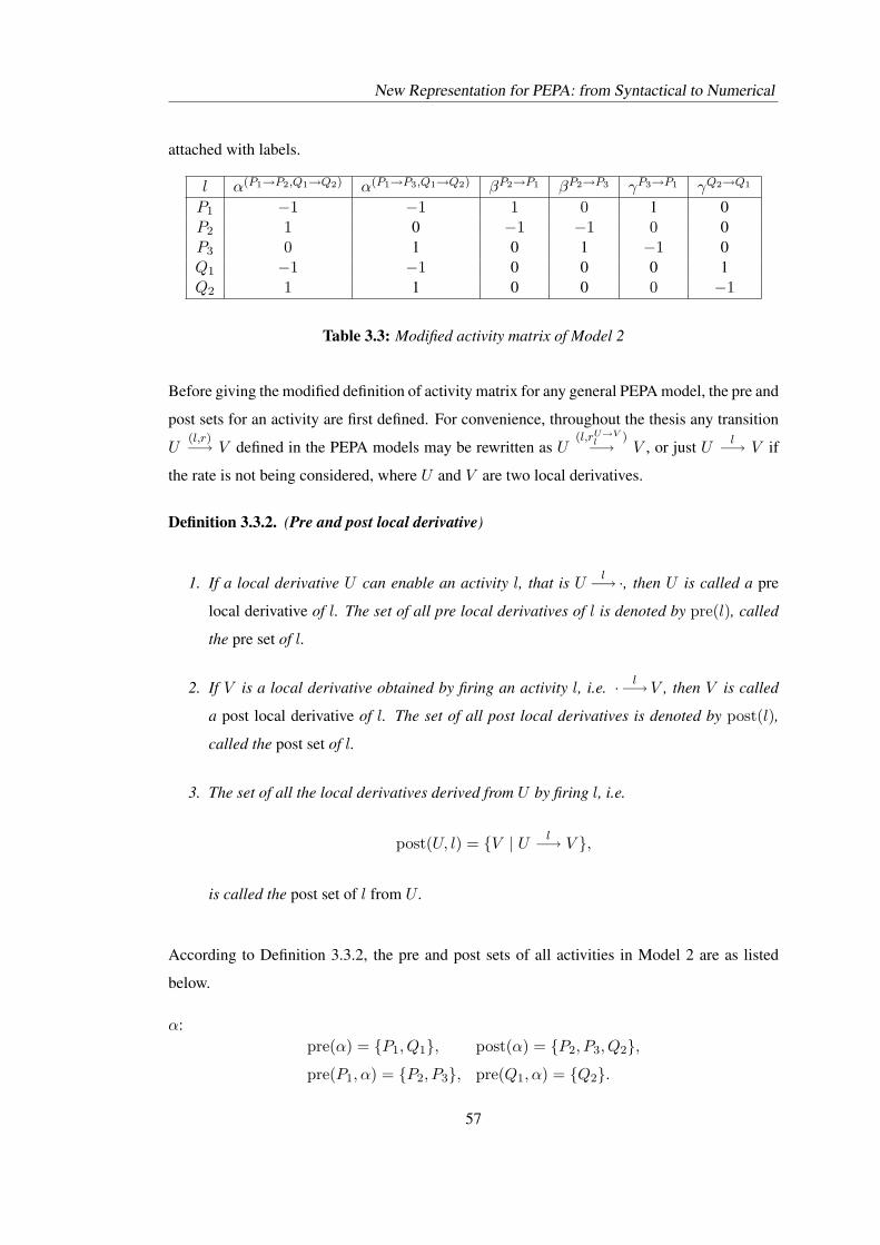
New Representation for PEPA: from Syntactical to Numerical
attached with labels.
l α(P1→P2,Q1→Q2) α(P1→P3,Q1→Q2) βP2→P1 βP2→P3 γP3→P1 γQ2→Q1
P1 −1 −1 1 0 1 0P2 1 0 −1 −1 0 0P3 0 1 0 1 −1 0Q1 −1 −1 0 0 0 1Q2 1 1 0 0 0 −1
Table 3.3: Modified activity matrix of Model 2
Before giving the modified definition of activity matrix for any general PEPA model, the pre and
post sets for an activity are first defined. For convenience, throughout the thesis any transition
U(l,r)−→ V defined in the PEPA models may be rewritten as U
(l,rU→Vl )−→ V , or just U
l−→ V if
the rate is not being considered, where U and V are two local derivatives.
Definition 3.3.2. (Pre and post local derivative)
1. If a local derivative U can enable an activity l, that is Ul−→·, then U is called a pre
local derivative of l. The set of all pre local derivatives of l is denoted by pre(l), called
the pre set of l.
2. If V is a local derivative obtained by firing an activity l, i.e. · l−→V , then V is called
a post local derivative of l. The set of all post local derivatives is denoted by post(l),
called the post set of l.
3. The set of all the local derivatives derived from U by firing l, i.e.
post(U, l) = {V | U l−→ V },
is called the post set of l from U .
According to Definition 3.3.2, the pre and post sets of all activities in Model 2 are as listed
below.
α:pre(α) = {P1, Q1}, post(α) = {P2, P3, Q2},
pre(P1, α) = {P2, P3}, pre(Q1, α) = {Q2}.
57
New Representation for PEPA: from Syntactical to Numerical
β:
pre(β) = {P2}, post(β) = post(P2, β) = {P1, P3}.
γ:pre(γ) = {P3, Q2}, post(γ) = {P1, Q1},
post(P3, γ) = {P1}, post(Q2, γ) = {Q1}.
Obviously, if l has only one pre local derivative, i.e. #pre(l) = 1, then l is an individual activity,
i.e. an activity that is not synchronised with other activities, like β in Model 2. But l being
individual does not imply #pre(l) = 1, see γ for instance. If l is shared, then #pre(l) > 1, for
example, see #pre(α) = #{P1, Q1} = 2. For a shared activity l with pre(l) = k, there are k
local derivatives that can enable this activity, each of them belonging to a distinct component
type. The obtained local derivatives are in the set post(pre(l)[i], l), where pre(l)[i] is the i-th
pre local derivative of l. But only one of them can be chosen after l is fired from pre(l)[i].
Since for the component type, namely i or Ci, there are #post(pre(l)[i], l) outputs, so the total
number of the distinct transitions for the whole system is
k∏i=1
#post(pre(l)[i], l).
That is, there are∏k
i=1 #post(pre(l)[i], l) possible results but only one of them can be chosen
by the system after the shared activity l is fired. In other words, to distinguish these possible
transitions, we need∏k
i=1 #post(pre(l)[i], l) different labels. Here are the readily accessible
labels:
(pre(l)[1] → V1,pre(l)[2] → V2, · · · ,pre(l)[k] → Vk),
where Vi ∈ post(pre(l)[i], l). Obviously, for each vector
(V1, V2, · · · , Vk) ∈ post(pre(l)[1], l)× post(pre(l)[2], l)× · · · × post(pre(l)[k], l),
the labelled activity l(pre(l)[1]→V1,pre(l)[2]→V2,··· ,pre(l)[k]→Vk) represents a distinct transition. For
example, α in Model 2 can be labelled as α(P1→P2,Q1→Q2) and α(P1→P3,Q1→Q2).
For an individual activity l, things are rather simple and easy: for U ∈ pre(l), l can be la-
belled as lU→post(U,l)[1], lU→post(U,l)[2], lU→post(U,l)[kU ], where kU = #post(U, l). Varying
U ∈ pre(l), there are∑
U∈pre(l) #post(U, l) labels needed to distinguish the possible transi-
58
New Representation for PEPA: from Syntactical to Numerical
tions. See βP2→P1 , βP2→P3 , γP3→P1 , γQ2→Q1 in Model 2 for instance. Now we give the formal
definition.
Definition 3.3.3. (Labelled Activity).
1. For any individual activity l, for each U ∈ pre(l), V ∈ post(U, l), label l as lU→V .
2. For a shared activity l, for each
(V1, V2, · · · , Vk) ∈ post(pre(l)[1], l)× post(pre(l)[2], l)× · · · × post(pre(l)[k], l),
label l as lw, where
w = (pre(l)[1] → V1,pre(l)[2] → V2, · · · ,pre(l)[k] → Vk).
Each lU→V or lw is called a labelled activity. The set of all labelled activities is denoted by
Alabel. For the above labelled activities lU→V and lw, their respective pre and post sets are
defined as
pre(lU→V ) = {U}, post(lU→V ) = {V },
pre(lw) = pre(l), post(lw) = {V1, V2, · · · , Vk}.
According to Definition 3.3.3, each lU→V or lw can only lead to a unique output. No new
activities are created, since labels are only attached to the activity to distinguish the results after
this activity is fired.
The impact of labelled activities on local derivatives can be recorded in a matrix form, as defined
below.
Definition 3.3.4. (Activity Matrix). For a model with NAlabellabelled activities and ND distinct
local derivatives, the activity matrix C is an ND ×NAlabelmatrix, and the entries are defined
as follows
C(Ui, lj) =
+1 if Ui ∈ post(lj)
−1 if Ui ∈ pre(lj)
0 otherwise
where lj is a labelled activity.
59
New Representation for PEPA: from Syntactical to Numerical
The modified activity matrix captures all the structural information, including the information
about choices and synchronisations, of a given PEPA model. From each row of the matrix,
which corresponds to each local derivative, we can know which activities this local derivative
can enable and after which activities are fired this local derivative can be derived. From the
perspective of the columns, the number of “−1”s in a column tells whether the corresponding
activity is synchronised or not. Only one “−1” means that this transition corresponds to an
individual activity. The locations of “−1” and “1” indicate which local derivatives can enable
the activity and what the derived local derivatives are, i.e. the pre and post local derivatives. In
addition, the numbers of “−1”s and “1”s in each column are the same, because any transition
in any component type corresponds to a unique pair of pre and post local derivatives. In fact, all
this information is also stored in the labels of the activities. Therefore, with the transition rate
functions defined in the next section to capture the timing information, a given PEPA model
can be recovered from its activity matrix.
Hereafter the terminology of activity matrix refers to the one in Definition 3.3.4. This definition
embodies the transition or operation rule of a given PEPA model, with the exception of timing
information. For a given PEPA model, each transition of the system results from the firing of
an activity. Each optional result after enabling this activity corresponds to a relevant labelled
activity, that is, corresponds to a column of the activity matrix. Conversely, each column of
the activity matrix corresponding to a labelled activity, represents an activity and the chosen
derived result after this activity is fired. So each column corresponds to a system transition.
Therefore, we have the following proposition, which specifies the correspondence between
system transitions and the columns of the activity matrix.
Proposition 3.3.1. Each column of the activity matrix corresponds to a system transition and
each transition can be represented by a column of the activity matrix.
As Proposition 3.3.1 reveals, the syntactically defined activity matrix provides the numerical
representation for the transitions between system states. Moreover, it is convenient for utilis-
ing mathematical techniques such as linear algebra and linear programming to investigate the
structural properties of PEPA models (see the next chapter for details).
An algorithm for automatically deriving the activity matrix from any PEPA model will be given
in the next section. For convenience, in the following we define the pre and post activity
matrices for PEPA, which can be directly obtained from the activity matrix.
60
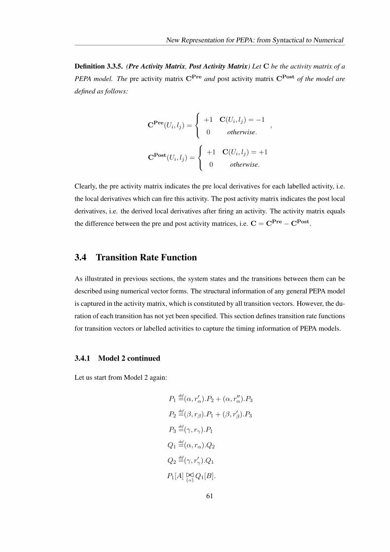
New Representation for PEPA: from Syntactical to Numerical
Definition 3.3.5. (Pre Activity Matrix, Post Activity Matrix) Let C be the activity matrix of a
PEPA model. The pre activity matrix CPre and post activity matrix CPost of the model are
defined as follows:
CPre(Ui, lj) =
+1 C(Ui, lj) = −1
0 otherwise.,
CPost(Ui, lj) =
+1 C(Ui, lj) = +1
0 otherwise.
Clearly, the pre activity matrix indicates the pre local derivatives for each labelled activity, i.e.
the local derivatives which can fire this activity. The post activity matrix indicates the post local
derivatives, i.e. the derived local derivatives after firing an activity. The activity matrix equals
the difference between the pre and post activity matrices, i.e. C = CPre −CPost.
3.4 Transition Rate Function
As illustrated in previous sections, the system states and the transitions between them can be
described using numerical vector forms. The structural information of any general PEPA model
is captured in the activity matrix, which is constituted by all transition vectors. However, the du-
ration of each transition has not yet been specified. This section defines transition rate functions
for transition vectors or labelled activities to capture the timing information of PEPA models.
3.4.1 Model 2 continued
Let us start from Model 2 again:
P1def=(α, r′α).P2 + (α, r′′α).P3
P2def=(β, rβ).P1 + (β, r′β).P3
P3def=(γ, rγ).P1
Q1def=(α, rα).Q2
Q2def=(γ, r′γ).Q1
P1[A] BC{α}
Q1[B].
61
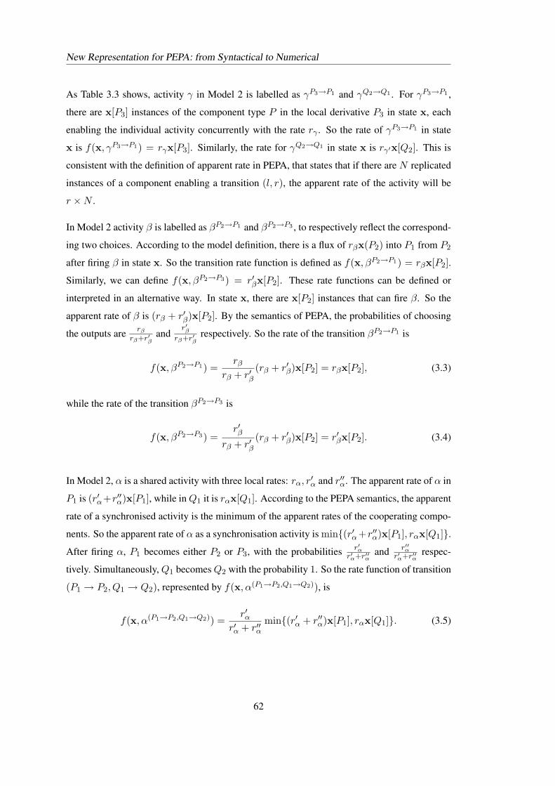
New Representation for PEPA: from Syntactical to Numerical
As Table 3.3 shows, activity γ in Model 2 is labelled as γP3→P1 and γQ2→Q1 . For γP3→P1 ,
there are x[P3] instances of the component type P in the local derivative P3 in state x, each
enabling the individual activity concurrently with the rate rγ . So the rate of γP3→P1 in state
x is f(x, γP3→P1) = rγx[P3]. Similarly, the rate for γQ2→Q1 in state x is rγ′x[Q2]. This is
consistent with the definition of apparent rate in PEPA, that states that if there are N replicated
instances of a component enabling a transition (l, r), the apparent rate of the activity will be
r ×N .
In Model 2 activity β is labelled as βP2→P1 and βP2→P3 , to respectively reflect the correspond-
ing two choices. According to the model definition, there is a flux of rβx(P2) into P1 from P2
after firing β in state x. So the transition rate function is defined as f(x, βP2→P1) = rβx[P2].
Similarly, we can define f(x, βP2→P3) = r′βx[P2]. These rate functions can be defined or
interpreted in an alternative way. In state x, there are x[P2] instances that can fire β. So the
apparent rate of β is (rβ + r′β)x[P2]. By the semantics of PEPA, the probabilities of choosing
the outputs are rβ
rβ+r′βand
r′βrβ+r′β
respectively. So the rate of the transition βP2→P1 is
f(x, βP2→P1) =rβ
rβ + r′β(rβ + r′β)x[P2] = rβx[P2], (3.3)
while the rate of the transition βP2→P3 is
f(x, βP2→P3) =r′β
rβ + r′β(rβ + r′β)x[P2] = r′βx[P2]. (3.4)
In Model 2, α is a shared activity with three local rates: rα, r′α and r′′α. The apparent rate of α in
P1 is (r′α+r′′α)x[P1], while in Q1 it is rαx[Q1]. According to the PEPA semantics, the apparent
rate of a synchronised activity is the minimum of the apparent rates of the cooperating compo-
nents. So the apparent rate of α as a synchronisation activity is min{(r′α +r′′α)x[P1], rαx[Q1]}.
After firing α, P1 becomes either P2 or P3, with the probabilities r′αr′α+r′′α
and r′′αr′α+r′′α
respec-
tively. Simultaneously, Q1 becomes Q2 with the probability 1. So the rate function of transition
(P1 → P2, Q1 → Q2), represented by f(x, α(P1→P2,Q1→Q2)), is
f(x, α(P1→P2,Q1→Q2)) =r′α
r′α + r′′αmin{(r′α + r′′α)x[P1], rαx[Q1]}. (3.5)
62
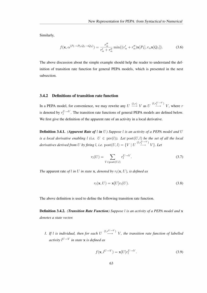
New Representation for PEPA: from Syntactical to Numerical
Similarly,
f(x, α(P1→P3,Q1→Q2)) =r′′α
r′α + r′′αmin{(r′α + r′′α)x[P1], rαx[Q1]}. (3.6)
The above discussion about the simple example should help the reader to understand the def-
inition of transition rate function for general PEPA models, which is presented in the next
subsection.
3.4.2 Definitions of transition rate function
In a PEPA model, for convenience, we may rewrite any U(l,r)−→ V as U
(l,rU→Vl )−→ V , where r
is denoted by rU→Vl . The transition rate functions of general PEPA models are defined below.
We first give the definition of the apparent rate of an activity in a local derivative.
Definition 3.4.1. (Apparent Rate of l in U ) Suppose l is an activity of a PEPA model and U
is a local derivative enabling l (i.e. U ∈ pre(l)). Let post(U, l) be the set of all the local
derivatives derived from U by firing l, i.e. post(U, l) = {V | U(l,rU→V
l )−→ V }. Let
rl(U) =∑
V ∈post(U,l)
rU→Vl . (3.7)
The apparent rate of l in U in state x, denoted by rl(x, U), is defined as
rl(x, U) = x[U ]rl(U). (3.8)
The above definition is used to define the following transition rate function.
Definition 3.4.2. (Transition Rate Function) Suppose l is an activity of a PEPA model and x
denotes a state vector.
1. If l is individual, then for each U(l,rU→V )−→ V , the transition rate function of labelled
activity lU→V in state x is defined as
f(x, lU→V ) = x[U ]rU→Vl . (3.9)
63
New Representation for PEPA: from Syntactical to Numerical
2. If l is synchronised, with pre(l) = {U1, U2, · · · , Uk}, then for each
(V1, V2, · · · , Vk) ∈ post(U1, l)× post(U2, l)× · · · × post(Uk, l),
let w = (U1 → V1, U2 → V2, · · · , Uk → Vk). Then the transition rate function of
labelled activity lw in state x is defined as
f(x, lw) =
(k∏
i=1
rUi→Vil
rl(Ui)
)min
i∈{1,··· ,k}{rl(x, Ui)},
where rl(x, Ui) = x[Ui]rl(Ui) is the apparent rate of l in Ui in state x. So
f(x, lw) =
(k∏
i=1
rUi→Vil
rl(Ui)
)min
i∈{1,··· ,k}{x[Ui]rl(Ui)}. (3.10)
Remark 3.4.1. Definition 3.4.2 accommodates the passive or unspecified rate >. If there are
some rU→Vl which are >, then the relevant calculation in the rate functions (3.9) and (3.10)
can be made according to the following inequalities and equations that define the comparison
and manipulation of unspecified activity rates (see Section 2.3.3 in Chapter 2):
r < w> for all r ∈ R+ and for all w ∈ N
w1> < w2> if w1 < w2 for all w1, w2 ∈ N
w1>+ w2> = (w1 + w2)> for all w1, w2 ∈ Nw1>w2> = w1
w2for all w1, w2 ∈ N
Moreover, we assume that 0 · > = 0. So the terms such as “min{A>, rB}” are interpreted
as [BGH07]:
min{A>, rB} =
rB, A > 0,
0, A = 0.
The definition of the transition rate function is consistent with the semantics of PEPA. We state
this result in a proposition.
Proposition 3.4.1. The transition rate function in Definition 3.4.2 is consistent with the opera-
tional semantics of PEPA.
The proof is given in Appendix B.1. Moreover, this kind of transition rate function has the
following properties.
64
New Representation for PEPA: from Syntactical to Numerical
Proposition 3.4.2. The transition rate function is nonnegative. If U is a pre local derivative of
l, i.e. U ∈ pre(l), then the transition rate function of l in a state x is less than the apparent rate
of l in U in this state, that is
0 ≤ f(x, l) ≤ rl(x, U) = x[U ]rl(U),
where rl(U) is the apparent rate of l in U for a single instance of U .
The proof is trivial and omitted.
Proposition 3.4.3. Let l be an labelled activity, and x,y be two states. The transition rate
function f(x, l) defined in Definition 3.4.2 satisfies:
1. For any H > 0, Hf(x/H, l) = f(x, l).
2. There exists M > 0 such that |f(x, l)− f(y, l)| ≤ M‖x− y‖ for any x,y and l.
Hereafter ‖ · ‖ denotes any matrix norm since all finite matrix norms are equivalent. For exam-
ple, we may define ‖A‖ =√∑
i,j a2ij for a matrix A = (aij). The first term of this proposition
illustrates a homogenous property of the rate function, while the second indicates the Lipschtiz
continuous property, both with respect to states. These characteristics will be utilised to in-
vestigate the fluid approximations of PEPA models in the following chapters. The proof of
Proposition 3.4.3 is given in Appendix B.2.
3.4.3 Algorithm for deriving activity matrix and transition rate functions
This section presents an algorithm for automatically deriving the activity matrix and rate func-
tions from any PEPA model, see Algorithm 1 (on page 66).
The lines 3-12 of Algorithm 1 deal with individual activities while lines 13−32 deal with shared
activities. The calculation methods in this algorithm are the embodiment of the definitions of
labelled activity and apparent rate as well as transition rate function. We would like to use an
example to illustrate this algorithm. Recall the discussion in Section 3.3.2 and 3.4.1. The shared
activity α in Model 2 is labelled as α(P1→P2,Q1→Q2) and α(P1→P3,Q1→Q2) with the following
corresponding transition rate functions respectively:
f(x, α(P1→P2,Q1→Q2)) =r′α
r′α + r′′αmin{(r′α + r′′α)x[P1], rαx[Q1]}, (3.11)
65
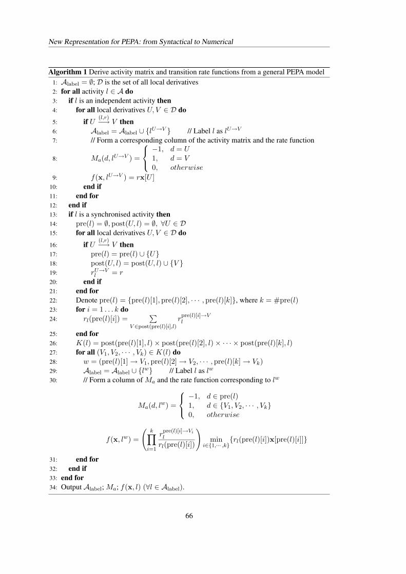
New Representation for PEPA: from Syntactical to Numerical
Algorithm 1 Derive activity matrix and transition rate functions from a general PEPA model1: Alabel = ∅; D is the set of all local derivatives2: for all activity l ∈ A do3: if l is an independent activity then4: for all local derivatives U, V ∈ D do5: if U
(l,r)−→ V then6: Alabel = Alabel ∪ {lU→V } // Label l as lU→V
7: // Form a corresponding column of the activity matrix and the rate function
8: Ma(d, lU→V ) =
−1, d = U1, d = V0, otherwise
9: f(x, lU→V ) = rx[U ]10: end if11: end for12: end if13: if l is a synchronised activity then14: pre(l) = ∅,post(U, l) = ∅, ∀U ∈ D15: for all local derivatives U, V ∈ D do16: if U
(l,r)−→ V then17: pre(l) = pre(l) ∪ {U}18: post(U, l) = post(U, l) ∪ {V }19: rU→V
l = r20: end if21: end for22: Denote pre(l) = {pre(l)[1],pre(l)[2], · · · ,pre(l)[k]}, where k = #pre(l)23: for i = 1 . . . k do24: rl(pre(l)[i]) =
∑V ∈post(pre(l)[i],l)
rpre(l)[i]→Vl
25: end for26: K(l) = post(pre(l)[1], l)× post(pre(l)[2], l)× · · · × post(pre(l)[k], l)27: for all (V1, V2, · · · , Vk) ∈ K(l) do28: w = (pre(l)[1] → V1,pre(l)[2] → V2, · · · ,pre(l)[k] → Vk)29: Alabel = Alabel ∪ {lw} // Label l as lw
30: // Form a column of Ma and the rate function corresponding to lw
Ma(d, lw) =
−1, d ∈ pre(l)1, d ∈ {V1, V2, · · · , Vk}0, otherwise
f(x, lw) =
(k∏
i=1
rpre(l)[i]→Vi
l
rl(pre(l)[i])
)min
i∈{1,··· ,k}{rl(pre(l)[i])x[pre(l)[i]]}
31: end for32: end if33: end for34: Output Alabel; Ma; f(x, l) (∀l ∈ Alabel).
66
New Representation for PEPA: from Syntactical to Numerical
f(x, α(P1→P3,Q1→Q2)) =r′′α
r′α + r′′αmin{(r′α + r′′α)x[P1], rαx[Q1]}. (3.12)
Now we show in detail how Algorithm 1 derives the labelled α, the corresponding columns of
the activity matrix, and the rate functions (3.11) and (3.12). Since α is a shared activity, let us
begin at Line 13 of the algorithm.
— First (by Lines 13− 21 of Algorithm 1),
pre(α) = {P1, Q1},
post(P1, α) = {P2, P3}, post(Q1, α) = {Q2},
and
rP1→P2α = r′α, rP1→P3
α = r′′α, rQ1→Q2α = rα.
— Then (by Lines 22− 26 of Algorithm 1),
rα(P1) = rP1→P2α + rP1→P3
α = r′α + r′′α,
rα(Q1) = rQ1→Q2α = rα,
and
K(α) = post(P1, α)× post(Q1, α) = {P2, P3} × {Q2}.
— Finally (by Lines 27 − 33 of Algorithm 1), since there are two labels for α: w1 and w2,
where w1 = (P1 → P2, Q1 → Q2) and w2 = (P1 → P3, Q1 → Q2). So
Ma(·, αw1) = (−1, 1, 0,−1, 1)T , Ma(·, αw1) = (−1, 0, 1,−1, 1)T .
f(x, αw1) =rP1→P2α
rα(P1)rQ1→Q2α
rα(Q1)min{rα(P1)x[P1], rα(Q1)x[Q1]}
=r′α
r′α + r′′αmin{(r′α + r′′α)x[P1], rαx[Q1]},
f(x, αw2) =rP1→P3α
rα(P1)rQ1→Q2α
rα(Q1)min{rα(P1)x[P1], rα(Q1)x[Q1]}
=r′′α
r′α + r′′αmin{(r′α + r′′α)x[P1], rαx[Q1]}.
67
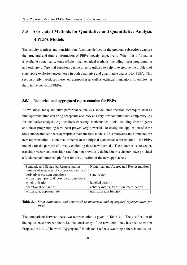
New Representation for PEPA: from Syntactical to Numerical
3.5 Associated Methods for Qualitative and Quantitative Analysis
of PEPA Models
The activity matrices and transition rate functions defined in the previous subsections capture
the structural and timing information of PEPA models respectively. When this information
is available numerically, some efficient mathematical methods, including linear programming
and ordinary differential equations can be directly utilised to help to overcome the problem of
state-space explosion encountered in both qualitative and quantitative analysis for PEPA. This
section briefly introduces these new approaches as well as technical foundations for employing
them in the context of PEPA.
3.5.1 Numerical and aggregated representation for PEPA
As we know, for quantitative performance analysis, model simplification techniques such as
fluid approximation can bring acceptable accuracy at a very low computational complexity. As
for qualitative analysis, e.g. deadlock checking, mathematical tools including linear algebra
and linear programming have been proven very powerful. Basically, the application of these
tools and techniques needs appropriate mathematical models. This motivates and stimulates the
new representation—numerical rather than the original syntactical representation—for PEPA
models, for the purpose of directly exploiting these new methods. The numerical state vector,
transition vector, and transition rate function previously defined in this chapter, have provided
a fundamental numerical platform for the utilisation of the new approaches.
Syntactic and Separated Representation Numerical and Aggregated Representationnumber of instances of components in localderivatives (system equation) state vectoraction type; pre and post local derivative;synchronisation labelled activityoperational semantics activity matrix, transition rate functionaction rate; apparent rate transition rate function
Table 3.4: From syntactical and separated to numerical and aggregated representation forPEPA
The comparison between these two representation is given in Table 3.4. The justification of
the equivalence between them, i.e. the consistency of the new definitions, has been shown in
Proposition 3.4.1. The word “Aggregated” in this table reflects two things: there is no distinc-
68
New Representation for PEPA: from Syntactical to Numerical
tion made between different instances of the same component type; the system states, and the
transitions between them represented by transition vectors, are considered holistically rather
than locally based on sequential components. “Numerical” in this table emphasises that the
system states, the transitions between the states, and the average duration of the transitions, are
represented numerically. Again, the main benefits brought by the new representation scheme
are the significant decrease of the size of the state space and the convenience for employing
new mathematical methods.
3.5.2 Place/Transition system
Overcoming the state-space explosion problem is the basic motivation and stimulation for de-
veloping new methods for PEPA. The state space of a model is the foundation for both qual-
itative and quantitative analysis. Typical qualitative problems which can be addressed based
on state-space related analysis include state space derivation and storage, deadlock checking,
etc. Generally, qualitative analysis is structure-related rather than timing-related. Since the
structural information has been numerically represented in activity matrices, it is possible and
feasible to do qualitative analysis such as deadlock-checking based on activity matrices directly,
and thus avoid the state-space explosion problem.
The numerical representation for system states and transitions, helps to find and manifest the
P/T structure underlying each PEPA model. Thus some powerful techniques and theories such
as linear algebra and linear programming developed for P/T systems [STC96] can be directly
utilised for the qualitative analysis of PEPA. In the next chapter, the readers will see that
through this approach, the derivation and storage of the state space of a class PEPA models will
no longer be a problem since the state space can be expressed using linear algebraic equations.
Moreover, structure-based rather than state-space-based theories and algorithms for deadlock
checking have been developed based on these equations. They are particularly efficient for large
scale systems with repeated components since they can avoid searching for deadlocks in the en-
tire state space. Further, a kind of interesting and useful structural property —invariance—has
been found in many PEPA models, which can be used to reason about the system. Of course,
the foundation for the applications of these new methods is the numerical and aggregated rep-
resentation for PEPA, which is already presented in this chapter. The detailed investigation and
discussion of the qualitative analysis of PEPA models will be given in the next chapter.
69
New Representation for PEPA: from Syntactical to Numerical
3.5.3 Aggregated CTMC and ODEs
As we have mentioned in Chapter 2, for each PEPA model, there is a CTMC underlying the
model. By solving the global balance equations associated with the infinitesimal generator of
this CTMC, the steady-state probability distribution can be obtained, from which performance
measures can be derived. According to the original definition of the PEPA language in which
each instance of the same component type is considered distinctly, the size of the state space of
this CTMC (called the original CTMC) may increase exponentially with the number of com-
ponents. Since there is no difference between components of the same type, the number rather
than the identity of the components in the local derivatives can be captured, introducing the
concept of numerical vector form to represent the system state, which results in the aggregated
CTMC. The size of the state space can thus be significantly reduced, as Proposition 3.2.1
shows, together with the computational complexity of deriving the performance by solving
the corresponding global balance equations since, the dimension of the infinitesimal generator
matrix is the square of the size of the state space.
Alternatively, the aggregated CTMC can be achieved by constructing a partition over the state
space of the original CTMC. In the aggregated CTMC, each partition of states in the original
CTMC forms a state, which can be represented by the numerical vector form as defined in
Definition 3.2.1. This partition is induced by an equivalence relation defined over the state
space of the original CTMC: the state s and s′ are equivalent if and only if the numbers of the
components in each local derivative at s and s′ are the same. The infinitesimal generator and
steady state distributions of the aggregated CTMC can also be formed from the ones of the
original CTMC. For detailed information of aggregation of Markov processes, please refer to
Section 5.4 in [Hil96].
Unless otherwise stated, hereafter the CTMC underlying a PEPA model refers to the aggregated
CTMC, and the state of a model or a system is considered in the sense of aggregation. As
discussed previously, a transition between states, namely from x to x + l, is represented by a
transition vector l corresponding to the labelled activity, namely l. The rate of the transition l
in state x is specified by the transition rate function f(x, l). That is,
x(l,f(x,l))−→ x + l.
Given a starting state x0, the transition chain corresponding to a firing sequence l0, l1, · · · , l, · · ·
70
New Representation for PEPA: from Syntactical to Numerical
is
x0(l0,f(x0,l0))−→ x0 + l0
(l1,f(x0+l0,l1))−→ (x0 + l0) + l1···−→· · · ···−→x
(l,f(x,l))−→ x + l···−→· · · .
The above sequence can be considered as one path or realisation of a simulation of the aggre-
gated CTMC, if the enabled activity at each state is chosen stochastically, i.e. is chosen through
the approach of sampling. After a long time, the steady-state of the system is assumed to be
achieved. The averaged occurrence number of an activity during one unit time, and the aver-
aged proportion of the number of components appearing in a local derivative can be calculated
from the simulation, which are referred to as the throughput of this activity and the utilisation
of the local state respectively. Moreover, given a starting state and a stopping state, the duration
between these two states, which is called response time, can be also obtained. In Chapter 7, we
will provide a stochastic simulation algorithm (Algorithm 3), which is based on our numerical
representation scheme, to derive these performance measures from PEPA models. The weak-
ness of the simulation method is its high computational cost, which makes it not suitable for
real-time performance monitoring or prediction. See Chapter 7 for a case study and detailed
discussions.
A promising approach for quantitative analysis of PEPA is fluid approximation, which brings
acceptable accuracy at a very low computational complexity for some models. The state space
of an underlying CTMC is inherently discrete, with the entries within the numerical vector form
always being non-negative integers and always being incremented or decremented in steps of
one. As pointed out in [Hil05a], when the numbers of components are large these steps are
relatively small and we can approximate the behaviour by considering the movement between
states to be continuous, rather than occurring in discontinuous jumps. This approach results in
a set of ODEs:dxdt
=∑
l∈Alabel
lf(x, l), (3.13)
where the vector x is short for x(t), representing the populations of components in local deriva-
tives at time t; and l is a transition vector while f(x, l) is a rate function.
These ODEs are immediately available as long as the activity matrix and the transition rate
functions are generated by Algorithm 1. The fluid approximation approach was first proposed
by Hillston in [Hil96] for a class of restricted PEPA models. The restrictions include: indi-
vidual activities must occur only once within derivative definitions and cannot appear within
71
New Representation for PEPA: from Syntactical to Numerical
different component definitions; shared activities cannot have different local rates, etc.. These
restrictions are relaxed here, since our derived ODEs (see (3.13)) only depend on the activity
matrix and transition rate functions, which are defined for general PEPA models. At this mo-
ment, there are some natural problems: does the ODE solution exist and is it unique? what
is the relationship between that solution and the CTMC? how to derive performance measures
from ODEs, etc. In the following chapters these problems will be discussed in detail.
3.6 Summary
This chapter has defined the labelled activities, activity matrices and transition rate functions for
PEPA, to capture the structural and timing information respectively. These definitions are used
to describe PEPA models numerically rather than syntactically. This numerical representation
scheme provides a platform for the direct application of some powerful mathematical tools
such as linear algebra, linear programming and ODEs, and non-mathematical methods such as
P/T theory, for the purpose of qualitative and quantitative analysis of large scale PEPA models.
Some fundamental properties of these definitions have been discussed and will be utilised for
further investigation of PEPA in the following chapters.
72
Chapter 4
Structural Analysis for PEPA Models
4.1 Introduction
Structural analysis provides an important route to gaining insight about how systems will per-
form qualitatively. However, the size and complexity of such systems challenge the capabilities
of the current approaches for structural analysis. For example, the current method to check
whether there is a deadlock in a PEPA model relies on exploring the entire state space of the
model. Therefore the computational complexity is mainly determined by the size of the state
space. For large scale PEPA models, particularly the models with more than ten million states,
even the derivation of the state space becomes impossible due to the state-space explosion
problem, let alone deadlock-checking for these models. This chapter will demonstrate a new
approach for structural analysis of PEPA, which avoids the state-space explosion problem.
The previous chapter has presented the definitions of numerical vectors and labelled activity,
activity matrix, as well as transition rate functions, for the PEPA language. These definitions
will closely relate PEPA to other formalisms such as Petri nets. Petri nets or P/T nets are an-
other modelling language which is widely used in the analysis of systems that exhibit complex
behaviour due to the interleaving of parallelism and synchronisation. In this chapter we will
show there is a P/T structure underlying each PEPA model. Based on the techniques developed
in the context of P/T systems in Petri nets, we will demonstrate how to find invariants and how
to efficiently derive and store the state space for large scale PEPA models. In particular, we will
present a structure-based deadlock-checking approach for PEPA which avoids the state-space
explosion problem.
The PEPA models considered in this chapter satisfy two assumptions: there is no cooperation
within groups of components of the same type; and each column of the activity matrix of a
model is distinct, i.e. each labelled activity is distinct in terms of pre and post local derivatives.
The remainder of this chapter is organised as follows: Section 2 presents the P/T structure
underlying PEPA models; Section 3 discusses how to derive invariants from PEPA models;
73
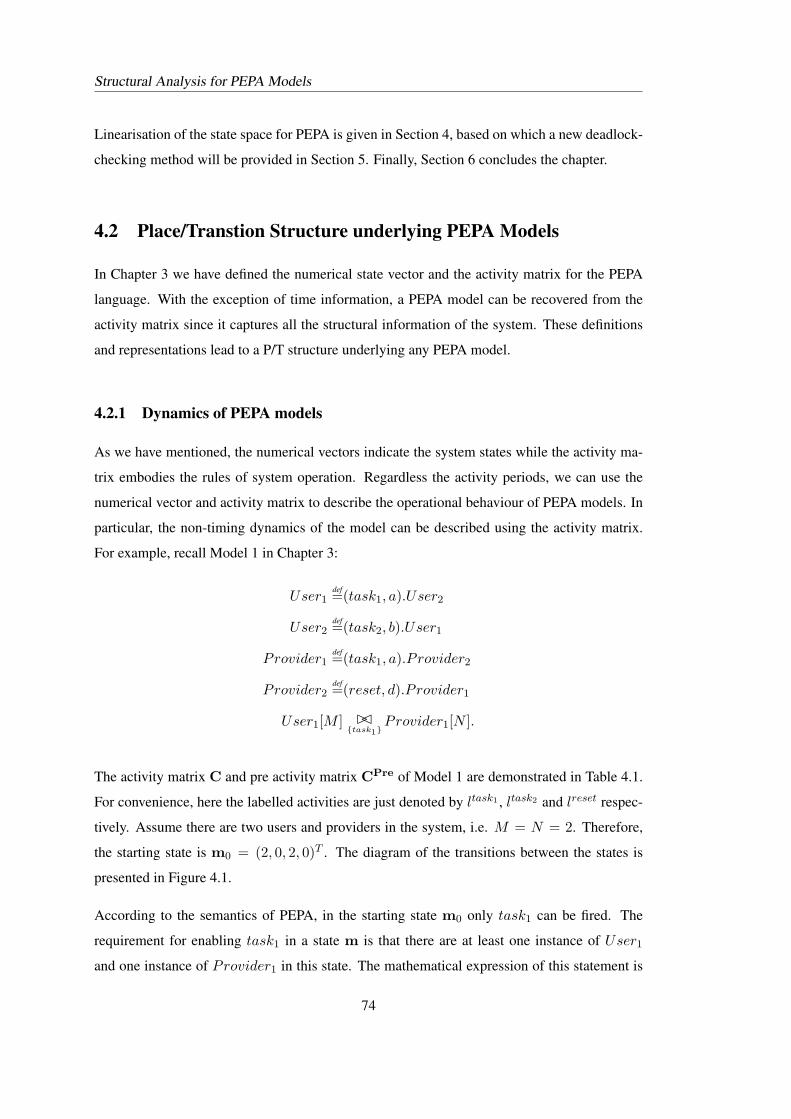
Structural Analysis for PEPA Models
Linearisation of the state space for PEPA is given in Section 4, based on which a new deadlock-
checking method will be provided in Section 5. Finally, Section 6 concludes the chapter.
4.2 Place/Transtion Structure underlying PEPA Models
In Chapter 3 we have defined the numerical state vector and the activity matrix for the PEPA
language. With the exception of time information, a PEPA model can be recovered from the
activity matrix since it captures all the structural information of the system. These definitions
and representations lead to a P/T structure underlying any PEPA model.
4.2.1 Dynamics of PEPA models
As we have mentioned, the numerical vectors indicate the system states while the activity ma-
trix embodies the rules of system operation. Regardless the activity periods, we can use the
numerical vector and activity matrix to describe the operational behaviour of PEPA models. In
particular, the non-timing dynamics of the model can be described using the activity matrix.
For example, recall Model 1 in Chapter 3:
User1def=(task1, a).User2
User2def=(task2, b).User1
Provider1def=(task1, a).P rovider2
Provider2def=(reset, d).P rovider1
User1[M ] BC{task1}
Provider1[N ].
The activity matrix C and pre activity matrix CPre of Model 1 are demonstrated in Table 4.1.
For convenience, here the labelled activities are just denoted by ltask1 , ltask2 and lreset respec-
tively. Assume there are two users and providers in the system, i.e. M = N = 2. Therefore,
the starting state is m0 = (2, 0, 2, 0)T . The diagram of the transitions between the states is
presented in Figure 4.1.
According to the semantics of PEPA, in the starting state m0 only task1 can be fired. The
requirement for enabling task1 in a state m is that there are at least one instance of User1
and one instance of Provider1 in this state. The mathematical expression of this statement is
74
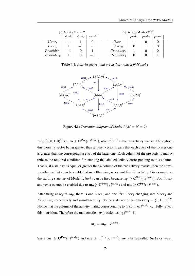
Structural Analysis for PEPA Models
(a) Activity Matrix C
ltask1 ltask2 lreset
User1 −1 1 0User2 1 −1 0
Provider1 −1 0 1Provider2 1 0 −1
(b) Activity Matrix CPre
ltask1 ltask2 lreset
User1 1 0 0User2 0 1 0
Provider1 1 0 0Provider2 0 0 1
Table 4.1: Activity matrix and pre activity matrix of Model 1
( )2,0,2,0 T
( )1,1,2,0 T
( )2,0,0,2 T
( )2,0,1,1 T
( )0,2,0,2 T
( )1,1,1,1 T
( )0,2,1,1 T( )1,1,0,2 T
( )0,2,2,0 T
task1
task1
task2
task2
reset
reset task2 reset
task1 task1
resettask2
task2
reset task2
reset
Figure 4.1: Transition diagram of Model 1 (M = N = 2)
m ≥ (1, 0, 1, 0)T , i.e. m ≥ CPre(·, ltask1), where CPre is the pre activity matrix. Throughout
this thesis, a vector being greater than another vector means that each entry of the former one
is greater than the corresponding entry of the latter one. Each column of the pre activity matrix
reflects the required condition for enabling the labelled activity corresponding to this column.
That is, if a state m is equal or greater than a column of the pre activity matrix, then the corre-
sponding activity can be enabled at m. Otherwise, m cannot fire this activity. For example, at
the starting state m0 of Model 1, task1 can be fired because m0 ≥ CPre(·, ltask1). Both task2
and reset cannot be enabled due to m0 � CPre(·, ltask2) and m0 � CPre(·, lreset).
After firing task1 at m0, there is one User1 and one Provider1 changing into User2 and
Provider2 respectively and simultaneously. So the state vector becomes m1 = (1, 1, 1, 1)T .
Notice that the column of the activity matrix corresponding to task1, i.e. ltask1 , can fully reflect
this transition. Therefore the mathematical expression using ltask1 is
m1 = m0 + ltask1.
Since m1 ≥ CPre(·, ltask2) and m1 ≥ CPre(·, lreset), m1 can fire either task2 or reset.
75
Structural Analysis for PEPA Models
Suppose task2 is fired, then we get m2 = (2, 0, 0, 1)T . That is
m2 = m1 + ltask2 = m0 + ltask1 + ltask2. (4.1)
Notice that each column of a matrix can be extracted by multiplying a corresponding vector at
the right side of this matrix:
ltask1 = C(1, 0, 0)T , ltask2 = C(0, 1, 0)T , lreset = C(0, 0, 1)T .
So (4.1) can be written as
m2 = m0 + ltask1 + ltask2 = m0 + C(1, 1, 0)T . (4.2)
Generally, the firing of a labelled activity l in state m yields the state m′, denoted by m l−→m′,
can be expressed as
m′ = m + C(·, l) (4.3)
where C(·, l) is the transition vector corresponding to l, i.e. the column of the activity matrix
that corresponds to l. If a firing sequence σ = l1 · · · lk · · · l ∈ Aωlabel from m0 yields the state
m, i.e.
m l1→m1 · · ·lk→mk · · ·
l→m,
then we denote m0σ→m. We define the firing count vector of a sequence σ as σ[l] = ](l, σ),
where ](l, σ) is the number of occurrences of l in σ. Integrating the evolution equation in (4.3)
from m0 to m we get:
m = m0 + C · σ. (4.4)
The formula (4.4) is called the state equation, reflecting that each state in the state space is
related to the starting state through an algebraic equation. This is consistent with the fact that
each system state results from the evolution of the system from the starting state. Of course,
the state equation does not involve the time information, so it cannot be used to do quantitative
analysis. However, for qualitative analysis of the system it is powerful.
76
Structural Analysis for PEPA Models
4.2.2 Place/Transition Structure in PEPA Models
Observe the activity matrix C in Table 4.1, each local derivative is in fact like a place and the
state vector records the population of components in each place, i.e. each local derivative. Each
transition vector, i.e. each column of the activity matrix represents the transition of components
from one place to another place. Such structure involving “place” and “transition” can be
formally defined. See the following concepts of P/T net and P/T system, which originate in
Petri net theory (“P/T” signifies “place/transition”) but they can also be interpreted in terms of
conditions and events.
Definition 4.2.1. (P/T net, Marking, P/T system, [CTS98])
1. A P/T net is a structure N = (P, T,Pre,Post) where: P and T are the sets of places
and transitions respectively; Pre and Post are the |P | × |T | sized, natural valued,
incidence matrices.
2. A marking is a vector m : P → N that assigns to each place of a P/T net a nonnegative
integer.
3. A P/T system is a pair S = 〈N ,m0〉: a net N with an initial marking m0.
In order to take advantage of the theory developed for P/T systems in the context of PEPA
models we must first establish the P/T system corresponding to a given PEPA model. This is
straightforward given the definitions presented in the previous chapter.
From Definition 4.2.1, it is easy to see that the structure N =(D,Alabel,CPre,CPost
)de-
rived from a PEPA model is a P/T net, where D,Alabel are the sets of all local derivatives and
all labelled activities of the PEPA model respectively, and CPre,CPost are the pre and post ac-
tivity matrices respectively. Given a starting state m0, S = 〈N ,m0〉 is a P/T system. Clearly,
each reachable marking m from m0 is a state of the aggregated CTMC underlying the given
PEPA model. This leads us to:
Theorem 4.2.1. There is a P/T system underlying any PEPA model, that is 〈N ,m0〉, where m0
is the starting state; N =(D,Alabel,CPre,CPost
)is P/T net: where D is the local derivative
set, Alabel is the labelled activity set; CPre and CPost are the pre and post activity matrices
respectively.
77
Structural Analysis for PEPA Models
Remark 4.2.1. Throughout this thesis, the P/T structure underlying a PEPA is referred to as
N =(D,Alabel,CPre,CPost
)or S = 〈N ,m0〉, which are constituted by the local derivative
and labelled activity sets, the pre activity matrix and post activity matrix, as well as the starting
state.
A P/T net, a particular class of Petri net, like PEPA provides a mathematical modelling language
for discrete, distributed systems. A Petri net or P/T net associated with time information, i.e. the
transitions are associated with time delays, is called a timed Petri net [Chi98] or a timed P/T net.
In particular, if the delays are random variables, usually satisfying exponentially distributions,
the timed Petri net is called a stochastic Petri net. In the PEPA language, the delay of a transition
l in a state m is specified by the transition rate function f(m, l) which are defined in Chapter 3.
For any given PEPA model, the underlying P/T net with incorporated transition rate functions
is obviously a stochastic Petri net.
In [Rib95] Ribaudo has defined a stochastic Petri net semantics for stochastic process alge-
bras, including PEPA. As in our work here, her approach associated each local derivative with
a place and each activity with a transition. To cope with the difference between action types
and transitions, she defined a labelling function that maps transition names into action names.
Similarly, our approach is to attach distinct labels to each action name, as indicated by the defi-
nition of labelled activity. However, since Ribaudo’s approach does not include aggregation as
we do, the mapping semantics in [Rib95] does not help with the state-space explosion problem
in structural analysis for large scale PEPA models with repeated components. In fact, since the
instances of the same component type are considered as distinct copies, their local derivatives
are consequently distinct. So the number of places will increase with the number of repeated
components, which is in contrast to the fixed number of places in our approach.
Moreover, our transition rate functions that capture the time information are defined on each
system state and each transition. Therefore, our approach is more convenient for quantitative
application, such as simulation and fluid approximation for PEPA models. Ribaudo’s work
was motivated by investigation into the relationship between formalisms whereas our work
is more application-oriented. We should point out that although our approach seems more
mathematical, the definitions of labelled activities and transition rate functions are essentially
syntactical.
Previous work on structural analysis of PEPA models in [GHR97] has some similarities with
78
Structural Analysis for PEPA Models
our approach. However, the class of PEPA considered in [GHR97] is somewhat restricted; in
particular no repeated components are allowed, which is also because no aggregation technique
is employed. Moreover, the problem of the difference between actions and transitions is not
considered. Furthermore, there is no time information considered in [GHR97], and therefore
their considerations cannot be extended to quantitative analysis. For convenience, some com-
parison between the work by different authors are presented in the following table.
Ribaudo [Rib95] Gilmore et al. [GHR97] This thesisMathematical representation No Yes YesSyntactical representation Yes No YesTime involved Yes No YesGenerality for PEPA Yes No YesAggregation technique No No YesDerivation algorithm No No YesSuitable for qualitative analysis No Yes YesSuitable for quantitative analysis No n/a YesSuitable for simulation No n/a Yes
Table 4.2: Comparison between three approaches
4.2.3 Some terminology
Now we introduce some terminology related to P/T systems for PEPA models (see [CTS98]
for reference). For convenience, if the concepts and conclusions that are defined and given for
P/T systems are used in the context of the PEPA language, they will be referred to as the P/T
structure underlying PEPA models.
As illustrated by the example in the last subsection, a transition l is enabled in a state m if
and only if m ≥ CPre[·, l]; its firing yields a new state m′ = m + C[·, l]. This fact is denoted
by ml→m′. We should point out that l is enabled in m can be equivalently stated using the
transition rate function f(m, l) defined in the previous chapter. In fact, we have a proposition:
Proposition 4.2.1. Let f(m, l) be the transition rate function given by Definition 3.4.2 in Chap-
ter 3, then
m ≥ CPre[·, l] ⇐⇒ f(m, l) > 0. (4.5)
Proof. Notice that l is a labelled activity. First, assume l is individual. Then l has only one pre
local derivative, namely U . So CPre[·, l] = eU , where eU is a vector with all entries being zeros
79
Structural Analysis for PEPA Models
except eU [U ] = 1. Thus m ≥ CPre[·, l] implies m[U ] ≥ eU [U ] = 1. By Definition 3.4.2,
f(m, l) = rm[U ] > 0, where r is a positive constant. Conversely, if f(m, l) = rm[U ] > 0,
then m[U ] > 0. Since each entry of a state vector is an integer, so we have m[U ] ≥ 1.
Therefore, m ≥ eU and thus m ≥ CPre[·, l].
Secondly, we assume l is a shared labelled activity with the pre set {U1, U2, · · · , Uk}. So
CPre[·, l] is such a vector e′ with all entries zero except e′[Ui] = 1, i = 1, 2, · · · , k. Therefore,
m ≥ CPre[·, l] implies m[Ui] ≥ e′[Ui] = 1. So f(m, l) > 0, where f(m, l) is given by (3.10)
in Definition 3.4.2, i.e.
f(m, l) =
(k∏
i=1
rUi→Vil
rl(Ui)
)min
i∈{1,··· ,k}{m[Ui]rl(Ui)},
where rUi→Vil , rl(Ui) are some positive constants. Conversely, f(m, l) > 0 implies m[Ui] ≥ 1
and thus implies m ≥ CPre[·, l].
According to this proposition, if f(m, l) = 0 then l cannot be enabled in m. That is,
m � CPre[·, l]. Therefore, a transition rate function not only specifies the rate of the ac-
tivity but also determines whether the activity can be enabled in a state. Since this chapter
emphasises structural rather than quantitative aspects of PEPA, we prefer to use the comparison
between the state vector and the column of the pre activity matrix, to determine whether a state
can enable an activity.
An occurrence sequence from m is a sequence of transitions σ = t1 · · · tk · · · such that
m t1→m1 · · ·tk→mk · · · . The language of S = 〈N ,m0〉, denoted by L(S) or L(N ,m0), is
the set of all the occurrence sequences from the starting state m0. A state m is said to be
reachable from m0 if there exists a σ in L(S) such that m0σ→m, that is
m = m0 + C · σ,
where σ is the firing count vector corresponding to σ. The set of all the reachable states from
m, called the reachability set from m, is denoted by RS(N ,m). According to the definition,
the reachability set of the P/T system S = 〈N ,m0〉 is
RS(N ,m0) ={m ∈ N|P | | ∃σ ∈ L(S) such that m = m0 + C · σ
},
80
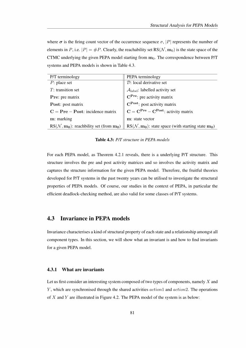
Structural Analysis for PEPA Models
where σ is the firing count vector of the occurrence sequence σ, |P | represents the number of
elements in P , i.e. |P | = #P . Clearly, the reachability set RS(N ,m0) is the state space of the
CTMC underlying the given PEPA model starting from m0. The correspondence between P/T
systems and PEPA models is shown in Table 4.3.
P/T terminology PEPA terminologyP : place set D: local derivative set
T : transition set Alabel: labelled activity set
Pre: pre matrix CPre: pre activity matrix
Post: post matrix CPost: post activity matrix
C = Pre−Post: incidence matrix C = CPre −CPost: activity matrix
m: marking m: state vector
RS(N ,m0): reachbility set (from m0) RS(N ,m0): state space (with starting state m0)
Table 4.3: P/T structure in PEPA models
For each PEPA model, as Theorem 4.2.1 reveals, there is a underlying P/T structure. This
structure involves the pre and post activity matrices and so involves the activity matrix and
captures the structure information for the given PEPA model. Therefore, the fruitful theories
developed for P/T systems in the past twenty years can be utilised to investigate the structural
properties of PEPA models. Of course, our studies in the context of PEPA, in particular the
efficient deadlock-checking method, are also valid for some classes of P/T systems.
4.3 Invariance in PEPA models
Invariance characterises a kind of structural property of each state and a relationship amongst all
component types. In this section, we will show what an invariant is and how to find invariants
for a given PEPA model.
4.3.1 What are invariants
Let us first consider an interesting system composed of two types of components, namely X and
Y , which are synchronised through the shared activities action1 and action2. The operations
of X and Y are illustrated in Figure 4.2. The PEPA model of the system is as below:
81
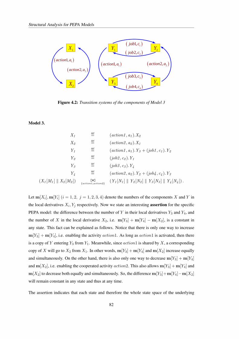
Structural Analysis for PEPA Models
( )11,action a
( )22,action a( )11,action a ( )22,action a
( )11,job c
( )22,job c
( )33,job c
( )44,job c
1X
2X
1Y 2Y
3Y 4Y
Figure 4.2: Transition systems of the components of Model 3
Model 3.
X1def= (action1 , a1 ).X2
X2def= (action2 , a2 ).X1
Y1def= (action1 , a1 ).Y3 + (job1 , c1 ).Y2
Y2def= (job2 , c2 ).Y1
Y3def= (job3 , c3 ).Y4
Y4def= (action2 , a2 ).Y2 + (job4 , c4 ).Y3
(X1 [M1 ] ‖ X2 [M2 ]) BC{action1,action2}
(Y1 [N1 ] ‖ Y2 [N2 ] ‖ Y3 [N3 ] ‖ Y4 [N4 ]) .
Let m[Xi],m[Yi] (i = 1, 2, j = 1, 2, 3, 4) denote the numbers of the components X and Y in
the local derivatives Xi, Yj respectively. Now we state an interesting assertion for the specific
PEPA model: the difference between the number of Y in their local derivatives Y3 and Y4, and
the number of X in the local derivative X2, i.e. m[Y3] + m[Y4] − m[X2], is a constant in
any state. This fact can be explained as follows. Notice that there is only one way to increase
m[Y3] + m[Y4], i.e. enabling the activity action1. As long as action1 is activated, then there
is a copy of Y entering Y3 from Y1. Meanwhile, since action1 is shared by X , a corresponding
copy of X will go to X2 from X1. In other words, m[Y3] +m[Y4] and m[X2] increase equally
and simultaneously. On the other hand, there is also only one way to decrease m[Y3] + m[Y4]
and m[X2], i.e. enabling the cooperated activity action2. This also allows m[Y3] +m[Y4] and
m[X2] to decrease both equally and simultaneously. So, the difference m[Y3]+m[Y4]−m[X2]
will remain constant in any state and thus at any time.
The assertion indicates that each state and therefore the whole state space of the underlying
82
Structural Analysis for PEPA Models
CTMC may have some interesting structural properties, such as invariants. A natural question
is how we can easily find all invariants in a general PEPA model. Before investigating this
problem, we need to define “invariant” first.
Definition 4.3.1. (Invariant) An invariant of a given PEPA model is a vector y ∈ Q such that
for any state m in the state space, yTm is a constant, or equivalently
yTm = yTm0, (4.6)
since the starting state m0 is a state and the constant is just yTm0.
The assertion discussed previously, i.e. “m[Y3] + m[Y4]−m[X2] is a constant”, can be illus-
trated by this definition. That is, y = (0,−1, 0, 0, 1, 1)T is an invariant of Model 3, since
yTm = m[Y3] + m[Y4]−m[X2] (4.7)
is a constant.
Once discovered, invariants may have potential applications such as model-based reasoning.
For example, based on the information on the server side, we may infer information about the
clients via an invariance relationship between them. For instance, by (4.7) and the number of
X2 we can know the numbers of Y in the local derivatives Y3 and Y4. In Chapter 7, a case
study shows how invariance can be used to prove the convergence of the fluid approximation of
PEPA models.
4.3.2 How to find invariants
In this subsection, we demonstrate how to find invariants in a given PEPA model. For any m in
the state space, there exists a corresponding sequence σ such that m = m0 + Cσ. Multiplying
both sides of this equation by yT , we have
yTm = yTm0 + yTCσ.
Obviously, yTm = yTm0 holds if and only if yTCσ = 0. Therefore, the following lemma is
ready.
Lemma 4.3.1. If yTC = 0, then y is an invariant.
83
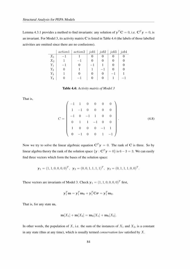
Structural Analysis for PEPA Models
Lemma 4.3.1 provides a method to find invariants: any solution of yTC = 0, i.e. CTy = 0, is
an invariant. For Model 3, its activity matrix C is listed in Table 4.4 (the labels of those labelled
activities are omitted since there are no confusions).
action1 action2 job1 job2 job3 job4X1 −1 1 0 0 0 0X2 1 −1 0 0 0 0Y1 −1 0 −1 1 0 0Y2 0 1 1 −1 0 0Y3 1 0 0 0 −1 1Y4 0 −1 0 0 1 −1
Table 4.4: Activity matrix of Model 3
That is,
C =
−1 1 0 0 0 0
1 −1 0 0 0 0
−1 0 −1 1 0 0
0 1 1 −1 0 0
1 0 0 0 −1 1
0 −1 0 0 1 −1
. (4.8)
Now we try to solve the linear algebraic equation CTy = 0. The rank of C is three. So by
linear algebra theory the rank of the solution space {y : CTy = 0} is 6− 3 = 3. We can easily
find three vectors which form the bases of the solution space:
y1 = (1, 1, 0, 0, 0, 0)T , y2 = (0, 0, 1, 1, 1, 1)T , y3 = (0, 1, 1, 1, 0, 0)T .
These vectors are invariants of Model 3. Check y1 = (1, 1, 0, 0, 0, 0)T first,
yT1 m = yT
1 m0 + yT1 Cσ = yT
1 m0.
That is, for any state m,
m[X1] + m[X2] = m0[X1] + m0[X2].
In other words, the population of X , i.e. the sum of the instances of X1 and X2, is a constant
in any state (thus at any time), which is usually termed conservation law satisfied by X .
84
Structural Analysis for PEPA Models
Similarly, y2 = (0, 0, 1, 1, 1, 1)T illustrates the conservation law satisfied by the component Y :
m[Y1]+m[Y2]+m[Y3]+m[Y4] is a constant for any state m. Moreover, y3 = (0, 1, 1, 1, 0, 0)T
means that for any state m,
m[X2] + m[Y1] + m[Y2]
is a constant. That is, the sum of the populations in X2, Y1 and Y2 always remains unchanged.
According to the definition of invariants, any linear combination of invariants is also an invari-
ant. For example, the following combination of y2 and y3:
y4 = y2 − y3 = (0,−1, 0, 0, 1, 1)T
is an invariant. Notice yT4 C = 0, which implies that
m[Y3] + m[Y4]−m[X2]
is a constant. This coincides with the assertion mentioned at the beginning of this section.
We should point out that yTC = 0 is not a necessary condition for some invariant y. For exam-
ple, consider Model 3 with m0 = (100, 0, 0, 0, 0, 3)T . Then the state space of the underlying
aggregated CTMC has four elements: m0 and
m1 = (100, 0, 0, 0, 1, 2)T , m2 = (100, 0, 0, 0, 2, 1)T , m3 = (100, 0, 0, 0, 3, 0)T .
y = (0, 1, 1, 0, 0, 0)T is an invariant since yTmk = 0 (k = 0, 1, 2, 3), but yTC 6= 0.
However, for a class of PEPA models, i.e. live PEPA models, the inverse of Lemma 4.3.1 is
true: y is an invariant can imply yTC = 0.
Definition 4.3.2. (Liveness for PEPA). Denote by 〈N ,m0〉 the P/T structure underlying a
given PEPA model.
1. A labelled activity l is live if for any derivative in the derivative set, there exists a se-
quence of activities such that the derivative after performing this sequence can perform
an l activity.
2. If all activities are live, then both 〈N ,m0〉 and the PEPA model are said to be live.
The liveness defined for PEPA is originally given for P/T nets (see [CTS98]). For some PEPA
85
Structural Analysis for PEPA Models
models, if they have no deadlocks then they are live, see Lemma 4.5.4 in this chapter. The
following proposition directly derives from a conclusion in P/T theory (page 319, [STC96]):
for a live P/T net yTC = 0 is equivalent to yTm = yTm0.
Proposition 4.3.1. If a given PEPA model is live, i.e. the underlying P/T structure⟨(D,Alabel,CPre,CPost
),m0
⟩is live, then for any state m in the state space,
yTC = 0 ⇐⇒ yTm = yTm0.
For the class of live PEPA models, finding invariants is much simpler—just solve the activity-
matrix-based linear algebric equation CyT = 0.
4.3.3 Conservation law as a kind of invariance
In the last subsection, we have seen that Model 3 satisfies a conservation laws, i.e. the popula-
tion of each component type is a constant in any state. In fact, this kind of conservation law is
universal for any PEPA model.
Let P be an arbitrary component type of a given PEPA model. The state transition of component
type P , i.e. any instance of P changing from one local derivative to another local derivative,
must occur within the set of P ’s local derivatives. That is, it is not possible to change into any
other component type’s local derivative. For an arbitrary labelled activity l, if there is a pre
local derivative of l, there must exist a post local derivative of l and this post local derivative
must be within component type P . Therefore, in each column of the activity matrix “1” and
“−1” must appear in a pair within the subvector corresponding to component type P . That is,
the sum of these “1” and “−1” within any component type is zero. So we have
Lemma 4.3.2. Let C be the activity matrix of a given PEPA model, D be the set of all local
derivatives. For an arbitrary component type P of this model, let DP be the local derivative
set of P . Define a vector yD with #D entries:
yP [U ] =
1 if U ∈ DP
0 if U ∈ D\DP
Then yTPC = 0.
Remark 4.3.1. Obviously, yP in Lemma 4.3.2 is an invariant by Lemma 4.3.1. Let P be the
86
Structural Analysis for PEPA Models
set of all component types of the given PEPA model. According to the definition of invariant,
a linear combination of invariants is also an invariant. So the sum∑
P∈P yP = 1 is also an
invariant. In fact, 1TC =∑
P∈P yTPC = 0.
Lemma 4.3.2 and Lemma 4.3.1 imply the following: the population of each component type and
therefore all component types in any state are constants. This fact is termed the conservation
law.
Proposition 4.3.2. (Conservation Law) For a given PEPA model, let D be the local derivative
set. For an arbitrary component type P ∈ P , let DP be the local derivative set of P . Then
∑U∈DP
m[U ] =∑
U∈DP
m0[U ]. (4.9)
∑U∈D
m[U ] =∑U∈D
m0[U ]. (4.10)
Proof. For any m, there exists a σ such that m = m0 + Cσ. By Lemma 4.3.2, yTPC = 0
where yTP is given in this lemma. So we have
∑U∈DP
m[U ] = yTPm = yT
P (m0 + Cσ) = yTPm0 =
∑U∈DP
m0[U ].
Moreover, let P be the set of all component types of this model, then
∑U∈D
m[U ] =∑P∈P
∑U∈DP
m[U ] =∑P∈P
∑U∈DP
m0[U ] =∑U∈D
m0[U ].
Proposition 4.3.2 can easily lead to the boundedness of the underlying state space.
Corollary 4.3.3. (Boundedness) The state space underlying a PEPA model is bounded: for
any state m and any local derivative U ,
0 ≤ m[U ] ≤ maxP∈P
∑U∈DP
m0[U ]
,
where P is the component type set, DP is the local derivative set corresponding to component
type P , m0 is the starting state.
87
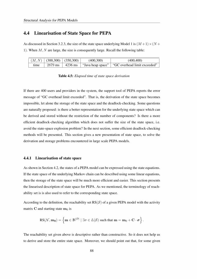
Structural Analysis for PEPA Models
4.4 Linearisation of State Space for PEPA
As discussed in Section 3.2.3, the size of the state space underlying Model 1 is (M +1)×(N +
1). When M,N are large, the size is consequently large. Recall the following table:
(M,N) (300,300) (350,300) (400,300) (400,400)time 2879 ms 4236 ms “Java heap space” “GC overhead limit exceeded”
Table 4.5: Elapsed time of state space derivation
If there are 400 users and providers in the system, the support tool of PEPA reports the error
message of “GC overhead limit exceeded”. That is, the derivation of the state space becomes
impossible, let alone the storage of the state space and the deadlock-checking. Some questions
are naturally proposed: is there a better representation for the underlying state space which can
be derived and stored without the restriction of the number of components? Is there a more
efficient deadlock-checking algorithm which does not suffer the size of the state space, i.e.
avoid the state-space explosion problem? In the next section, some efficient deadlock-checking
methods will be presented. This section gives a new presentation of state space, to solve the
derivation and storage problems encountered in large scale PEPA models.
4.4.1 Linearisation of state space
As shown in Section 4.2, the states of a PEPA model can be expressed using the state equations.
If the state space of the underlying Markov chain can be described using some linear equations,
then the storage of the state space will be much more efficient and easier. This section presents
the linearised description of state space for PEPA. As we mentioned, the terminology of reach-
ability set is is also used to refer to the corresponding state space.
According to the definition, the reachability set RS(S) of a given PEPA model with the activity
matrix C and starting state m0 is
RS(N ,m0) ={m ∈ N|D| | ∃σ ∈ L(S) such that m = m0 + C · σ
}.
The reachability set given above is descriptive rather than constructive. So it does not help us
to derive and store the entire state space. Moreover, we should point out that, for some given
88
Structural Analysis for PEPA Models
σ ∈ N|D|, m = m0 + Cσ ∈ N|D| may not be valid states because there may be no valid oc-
currence sequences corresponding to these σ. However m is said to belong to a generalisation
of the reachability set: the linearised reachability set. Before giving these definitions, we first
define some kind of flow and semiflow in the context of PEPA. (For the definitions of these
concepts in the context of P/T systems, see [CTS98]).
Definition 4.4.1. (Flow, Semiflow, Conservative and Consistent). Let C be the activity matrix
of a given PEPA model with the underlying P/T structure⟨(D,Alabel,CPre,CPost
),m0
⟩.
1. A p-flow is a vector y : D → Q such that yTC = 0. Natural and nonnegative flows are
called semiflows: vectors y : D → N such that yTC = 0. The model is conservative if
there exists a p-semiflow whose support covers D, that is {U ∈ D | y[U ] > 0} = D.
2. A basis (respectively, fundamental set) of p-flows (respectively p-semiflows),
B = {y1,y2, · · · ,yq} (respectively, Φ = {y1,y2, · · · ,yq}) is a minimal subset which
will generate any p-flow (respectively, p-semiflow) as follows: y =∑
yj∈Ψ kjyj , kj ∈
Q.
3. A t-flow is a vector x : Alabel → Q such that Cx = 0. Natural and nonnegative flows
are called semiflows: vectors x : Alabel → N such that Cx = 0. The model is consistent
if there exists a t-semiflow whose support covers Alabel.
By Proposition 4.3.2, any PEPA model is conservative. Obviously, a p-semiflow is a special
kind of p-flow while a t-semiflow is a special t-flow. Moreover, according to Lemma 4.3.1, a
p-flow is an invariant.
Let B and Φ be a basis of p-flows and a fundamental set of p-semiflows respectively. Then
for any m ∈ RS(N ,m0), we have Bm = 0 and Φm = 0. However this does not imply that
any m ∈ N|D| that satisfies Bm = 0 or Φm = 0 is in RS(N ,m0). But they do belong to
generalised reachability sets. See the following definitions.
Definition 4.4.2. (Linearised Reachability Set, [STC96]) Let S be a P/T system.
1. Its linearised reachability set using the state equation is defined as
LRSSE(S) ={m ∈ N|P | | ∃σ ∈ N|T | such that m = m0 + C · σ
}.
89
Structural Analysis for PEPA Models
2. Its linearised reachability set using the state equation over reals is defined as
LRSSER(S) ={m ∈ N|P | | ∃σ ≥ 0 such that m = m0 + C · σ
}.
3. Its linearised reachability set using a basis B of p-flows is defined as
LRSPf(S) ={m ∈ N|P | | B ·m = B ·m0
}.
4. Its linearised reachability set using a fundamental set of p-semiflows is defined as
LRSPsf(S) ={m ∈ N|P | | Φ ·m = Φ ·m0
}.
All the sets defined above are characterised using linear algebraic equations which makes the
set structure simpler. The job of determining whether a state belongs to a set is reduced to
verifying the equations.
Obviously, RS(S) ⊆ LRSSE(S). The difference between the definitions of LRSSE(S) and
LRSSER(S) is embodied in the different conditions imposed on σ. There is no doubt that
LRSSE(S) ⊆ LRSSER(S). Since for any m ∈ LRSSER(S), m = m0 + C · σ, then
Bm = Bm0 + BC · σ = Bm0,
so m ∈ LRSPf(S) and thus LRSSER(S) ⊆ LRSPf(S). The definitions of LRSPf(S) and
LRSPsf(S) are directly related to the invariants in the system. Clearly, LRSPf(S) ⊆ LRSPsf(S).
The relationships between these reachability sets are shown in the following lemmas.
Lemma 4.4.1. [STC96]. Let S be a P/T system, then
1. RS(S) ⊆ LRSSE(S) ⊆ LRSSER(S) ⊆ LRSPf(S) ⊆ LRSPsf(S).
2. If N is conservative, then LRSPf(S) = LRSPsf(S).
3. If N is consistent, then LRSSER(S) = LRSPf(S).
For the P/T structure S underlying a given PEPA model, we will see LRSSE(S) = LRSSER(S).
Lemma 4.4.2. Let S be the P/T system underlying a PEPA model.
LRSSE(S) = LRSSER(S).
90
Structural Analysis for PEPA Models
Proof. For any m ∈ LRSSER(S), there exists σ ≥ 0, such that m = m0 + C · σ. Notice
m,m0 ∈ N|D|, all elements of C are either−1, 0 or 1, and the assumption that each column of
C is distinct. So all elements of σ must be integers. Since σ ≥ 0, thus σ ∈ N|Alabel|. That is
m ∈ LRSSE(S). So LRSSE(S) ⊃ LRSSER(S). Since LRSSE(S) ⊂ LRSSER(S), therefore
LRSSE(S) = LRSSER(S).
We should point out that this proof is based on the assumption of distinct columns of the activity
matrix. However, this assumption can be relaxed for the analysis of state space. If there are
two columns the same, i.e. the two corresponding labelled activities have the same pre and post
local derivatives, we can modify the model in this way: combine these two labelled activities
into one. The activity matrix of the modified model then satisfies the assumption. But the state
space of the modified model as well as the associated transition relationship without timing
information, is the same as the original one. So the structural analysis based on the new state
space is the same as the analysis based on the original state space.
Now we introduce the concept of equal conflict (see [CTS98]).
Definition 4.4.3. (Equal Conflict) Let N = (P, T,Pre,Post) be a P/T net.
1. The P/T net N is called equal conflict (EQ), if pre(l) ∩ pre(l′) 6= ∅ implies Pre[·, l] =
Pre[·, l′].
2. The P/T net N is ordinary if each entry of Pre and Post is either zero or one.
3. An ordinary EQ net is a free choice (FC) net.
4. A PEPA model is called an EQ model if the P/T net underlying this model is EQ.
The following proposition will give an equivalent statement for an EQ PEPA model.
Proposition 4.4.1. For a PEPA model, we have
1. A PEPA model is an EQ model if and only if for any two labelled activities l and l′, their
pre sets are either equal or distinct, i.e., either pre(l) ∩ pre(l′) = ∅ or pre(l) = pre(l′).
2. An EQ PEPA model is a FC model.
91
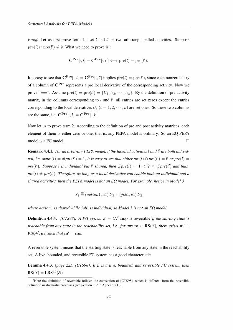
Structural Analysis for PEPA Models
Proof. Let us first prove term 1. Let l and l′ be two arbitrary labelled activities. Suppose
pre(l) ∩ pre(l′) 6= ∅. What we need to prove is :
CPre[·, l] = CPre[·, l′] ⇐⇒ pre(l) = pre(l′).
It is easy to see that CPre[·, l] = CPre[·, l′] implies pre(l) = pre(l′), since each nonzero entry
of a column of CPre represents a pre local derivative of the corresponding activity. Now we
prove “⇐=”. Assume pre(l) = pre(l′) = {U1, U2, · · · , Uk}. By the definition of pre activity
matrix, in the columns corresponding to l and l′, all entries are set zeros except the entries
corresponding to the local derivatives Ui (i = 1, 2, · · · , k) are set ones. So these two columns
are the same, i.e. CPre[·, l] = CPre[·, l′].
Now let us to prove term 2. According to the definition of pre and post activity matrices, each
element of them is either zero or one, that is, any PEPA model is ordinary. So an EQ PEPA
model is a FC model.
Remark 4.4.1. For an arbitrary PEPA model, if the labelled activities l and l′ are both individ-
ual, i.e. #pre(l) = #pre(l′) = 1, it is easy to see that either pre(l) ∩ pre(l′) = ∅ or pre(l) =
pre(l′). Suppose l is individual but l′ shared, then #pre(l) = 1 < 2 ≤ #pre(l′) and thus
pre(l) 6= pre(l′). Therefore, as long as a local derivative can enable both an individual and a
shared activities, then the PEPA model is not an EQ model. For example, notice in Model 3
Y1def= (action1, a1).Y3 + (job1, c1).Y2
where action1 is shared while job1 is individual, so Model 3 is not an EQ model.
Definition 4.4.4. [CTS98]. A P/T system S = 〈N ,m0〉 is reversible1if the starting state is
reachable from any state in the reachability set, i.e., for any m ∈ RS(S), there exists m′ ∈
RS(N ,m) such that m′ = m0.
A reversible system means that the starting state is reachable from any state in the reachability
set. A live, bounded, and reversible FC system has a good characteristic.
Lemma 4.4.3. (page 225, [CTS98]) If S is a live, bounded, and reversible FC system, then
RS(S) = LRSSE(S).1Here the definition of reversible follows the convention of [CTS98], which is different from the reversible
definition in stochastic processes (see Section C.2 in Appendix C).
92
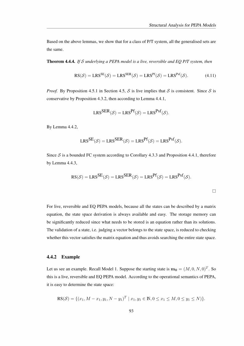
Structural Analysis for PEPA Models
Based on the above lemmas, we show that for a class of P/T system, all the generalised sets are
the same.
Theorem 4.4.4. If S underlying a PEPA model is a live, reversible and EQ P/T system, then
RS(S) = LRSSE(S) = LRSSER(S) = LRSPf(S) = LRSPsf(S). (4.11)
Proof. By Proposition 4.5.1 in Section 4.5, S is live implies that S is consistent. Since S is
conservative by Proposition 4.3.2, then according to Lemma 4.4.1,
LRSSER(S) = LRSPf(S) = LRSPsf(S).
By Lemma 4.4.2,
LRSSE(S) = LRSSER(S) = LRSPf(S) = LRSPsf(S).
Since S is a bounded FC system according to Corollary 4.3.3 and Proposition 4.4.1, therefore
by Lemma 4.4.3,
RS(S) = LRSSE(S) = LRSSER(S) = LRSPf(S) = LRSPsf(S).
For live, reversible and EQ PEPA models, because all the states can be described by a matrix
equation, the state space derivation is always available and easy. The storage memory can
be significantly reduced since what needs to be stored is an equation rather than its solutions.
The validation of a state, i.e. judging a vector belongs to the state space, is reduced to checking
whether this vector satisfies the matrix equation and thus avoids searching the entire state space.
4.4.2 Example
Let us see an example. Recall Model 1. Suppose the starting state is m0 = (M, 0, N, 0)T . So
this is a live, reversible and EQ PEPA model. According to the operational semantics of PEPA,
it is easy to determine the state space:
RS(S) = {(x1,M − x1, y1, N − y1)T | x1, y1 ∈ N, 0 ≤ x1 ≤ M, 0 ≤ y1 ≤ N)}.
93
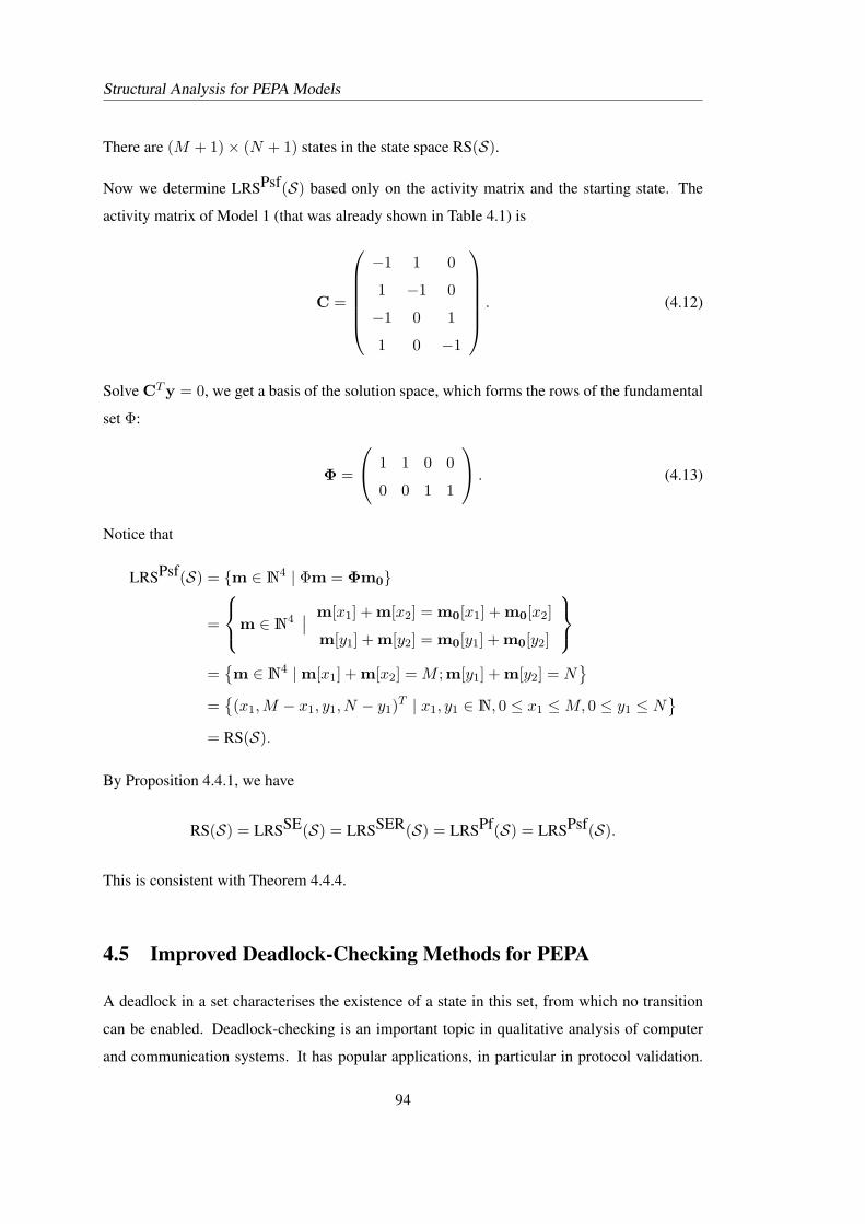
Structural Analysis for PEPA Models
There are (M + 1)× (N + 1) states in the state space RS(S).
Now we determine LRSPsf(S) based only on the activity matrix and the starting state. The
activity matrix of Model 1 (that was already shown in Table 4.1) is
C =
−1 1 0
1 −1 0
−1 0 1
1 0 −1
. (4.12)
Solve CTy = 0, we get a basis of the solution space, which forms the rows of the fundamental
set Φ:
Φ =
1 1 0 0
0 0 1 1
. (4.13)
Notice that
LRSPsf(S) = {m ∈ N4 | Φm = Φm0}
=
m ∈ N4∣∣ m[x1] + m[x2] = m0[x1] + m0[x2]
m[y1] + m[y2] = m0[y1] + m0[y2]
={m ∈ N4 | m[x1] + m[x2] = M ;m[y1] + m[y2] = N
}={(x1,M − x1, y1, N − y1)T | x1, y1 ∈ N, 0 ≤ x1 ≤ M, 0 ≤ y1 ≤ N
}= RS(S).
By Proposition 4.4.1, we have
RS(S) = LRSSE(S) = LRSSER(S) = LRSPf(S) = LRSPsf(S).
This is consistent with Theorem 4.4.4.
4.5 Improved Deadlock-Checking Methods for PEPA
A deadlock in a set characterises the existence of a state in this set, from which no transition
can be enabled. Deadlock-checking is an important topic in qualitative analysis of computer
and communication systems. It has popular applications, in particular in protocol validation.
94
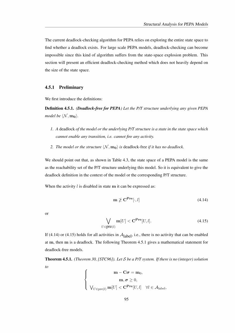
Structural Analysis for PEPA Models
The current deadlock-checking algorithm for PEPA relies on exploring the entire state space to
find whether a deadlock exists. For large scale PEPA models, deadlock-checking can become
impossible since this kind of algorithm suffers from the state-space explosion problem. This
section will present an efficient deadlock-checking method which does not heavily depend on
the size of the state space.
4.5.1 Preliminary
We first introduce the definitions:
Definition 4.5.1. (Deadlock-free for PEPA) Let the P/T structure underlying any given PEPA
model be 〈N ,m0〉.
1. A deadlock of the model or the underlying P/T structure is a state in the state space which
cannot enable any transition, i.e. cannot fire any activity.
2. The model or the structure 〈N ,m0〉 is deadlock-free if it has no deadlock.
We should point out that, as shown in Table 4.3, the state space of a PEPA model is the same
as the reachability set of the P/T structure underlying this model. So it is equivalent to give the
deadlock definition in the context of the model or the corresponding P/T structure.
When the activity l is disabled in state m it can be expressed as:
m � CPre[·, l] (4.14)
or ∨U∈pre(l)
m[U ] < CPre[U, l]. (4.15)
If (4.14) or (4.15) holds for all activities in Alabel, i.e., there is no activity that can be enabled
at m, then m is a deadlock. The following Theorem 4.5.1 gives a mathematical statement for
deadlock-free models.
Theorem 4.5.1. (Theorem 30, [STC96]). Let S be a P/T system. If there is no (integer) solution
to m−Cσ = m0,
m,σ ≥ 0,∨U∈pre(l) m[U ] < CPre[U, l] ∀l ∈ Alabel,
95
Structural Analysis for PEPA Models
then S is deadlock-free.
According to this theorem, to decide whether there is a deadlock, it is necessary to compare
each state in the state space to each column of the pre activity matrix. This is not an efficient
way to find a deadlock, especially for large scale PEPA models.∨U∈pre(l) m[U ] < CPre[U, l] means that there exists U such that m[U ] < CPre[U, l]. Notice
that all elements of m are nonnegative integers, and any entry of CPre[U, l] other than 1 is zero
for all U and l. So
m[U ] < CPre[U, l] ⇐⇒ m[U ] = 0 and CPre[U, l] = 1.
Of course, m ≥ 1 cannot be a deadlock, since m ≥ CPre[·, l] for any l. Thus, only a state
m with zeros in some particular places can possibly be a deadlock. This observation is very
helpful but not enough for deadlock-checking. All such states with zeros in some entries, have
to be found for checking, which is not always feasible especially in the situation of the state
space derivation or storage being a problem. Theorem 4.4.4 specifies the structure of the state
space, but it requires the condition of “liveness” in advance, which has already guaranteed the
deadlock-freeness.
In the following first subsection, an equivalent deadlock-checking theorem for a class of PEPA
models is illustrated, which allows equivalent deadlock-checking in the linearised state space.
The second subsection illustrates an efficient checking algorithm with some examples.
4.5.2 Equivalent deadlock-checking
Before stating our main results, we first list several lemmas which are used in the proof of our
theorem.
The reachability set of a P/T net is in fact a directed graph, i.e., each state is a node, the transition
from a state to another state is essentially a directed edge between two nodes. A directed graph
is called strongly connected if it contains a directed path from u to v and a directed path from v
to u for every pair of vertices u, v. A graph is called connected if every pair of distinct vertices
in the graph can be connected through some path. Obviously, a strongly connected graph is a
connected graph. The two definitions have been introduced to nets (see [MR80]). For a net, the
96
Structural Analysis for PEPA Models
following lemma provides two sufficient conditions of strongly connected.
Lemma 4.5.2. (Property 6.10, page 217, [CTS98]) Let N be a graph and C its incidence
matrix.
1. If N is connected, consistent and conservative, then it is strongly connected.
2. If N is live and bounded then it is strongly connected and consistent.
If N is the P/T net underlying a PEPA model, these conditions can be simplified.
Proposition 4.5.1. Suppose S = 〈N ,m0〉 be a P/T system underlying a PEPA model.
1. If N is consistent, then the state space is strongly connected.
2. If S is live, then N is strongly connected and consistent.
Proof. By Proposition 4.3.2 and Corollary 4.3.3 the P/T systems underlying PEPA models
are conservative and bounded. Notice that each state in the state space is reachable from the
initial state, i.e. the state space is connected. So according to Lemma 4.5.2, Proposition 4.5.1
holds.
Lemma 4.5.3. (Theorem 6.19, page 223, [CTS98]) Let S be a bounded strongly connected EQ
system. Then S is live iff it is deadlock-free.
Lemma 4.5.4. (Theorem 6.22, page 225, [CTS98]) If S is a live EQ system, then for any
ma, mb ∈ LRSSE(S), RS(N ,ma) ∩ RS(N ,mb) 6= ∅.
This lemma implies that there are no spurious deadlocks in live EQ systems, i.e. there are no
deadlocks in LRSSE(S).
Theorem 4.5.5. If the P/T structure S underlying a PEPA model is a consistent, EQ system,
then
1. LRSSE(S) is deadlock-free ⇐⇒ RS(S) is deadlock-free.
2. LRSSER(S) is deadlock-free ⇐⇒ RS(S) is deadlock-free.
3. LRSPf(S) is deadlock-free ⇐⇒ RS(S) is deadlock-free.
97
Structural Analysis for PEPA Models
4. LRSPsf(S) is deadlock-free ⇐⇒ RS(S) is deadlock-free.
Proof. It is easy to see that all “=⇒” holds because
LRSPsf(S) ⊃ LRSPf(S) ⊃ LRSSER(S) ⊃ LRSSE(S) ⊃ RS(S).
Now we show that each “⇐=” holds. Notice S is consistent, by Proposition 4.5.1, S is strongly
connected. Then according to Lemma 4.5.3, RS(S) is deadlock-free implies that S is live.
Since S is an EQ system, then by Lemma 4.5.4, LRSSE(S) is deadlock-free. Since now we
have LRSSE(S) = LRSSER(S) by Lemma 4.4.2, so LRSSER(S) is deadlock-free. Notice
by Lemma 4.4.1, the conservativeness and consistence of the system imply that LRSPf(S) =
LRSPsf(S) = LRSSER(S). So LRSPf(S) and LRSPsf(S) are deadlock-free.
Theorem 4.5.5 allows us to check the corresponding linearised state space to determine whether
a consistent and EQ model has deadlocks. We should point out that “consistent” and “EQ” can
be efficiently checked as properties of the activity matrix.
4.5.3 Deadlock-checking algorithm in LRSPsf
According to Theorem 4.5.5, for a consistent, EQ system S, to tell whether RS(S) has dead-
locks it is sufficient to check whether LRSPsf(S) has deadlocks.
As we mentioned, the activity l is disabled in m means that there exists a U such that m[U ] <
CPre[U, l]. Because
m[U ] < CPre[U, l] ⇐⇒ m[U ] = 0 and CPre[U, l] = 1,
so only the state m with zeros in some particular places can possibly be a deadlock. Based on
this idea, we provide a deadlock-checking algorithm, see Algorithm 2. In this algorithm, K(l) is
the set of vectors that cannot enable l. The intersected set of all K(l), i.e. K =⋂
l∈AlabelK(l),
is the deadlock candidate set, in which each vector cannot fire any activity. K⋂
LRSPsf is
used to check whether the deadlock candidates are in the linearised state space LRSPsf.
Since this algorithm depends on the system structure rather than the repeat instances of the com-
ponents, so does its computational complexity. Therefore, it is efficient for large scale systems
with repeated components. Our deadlock-checking algorithm is structure- or equation-based,
98
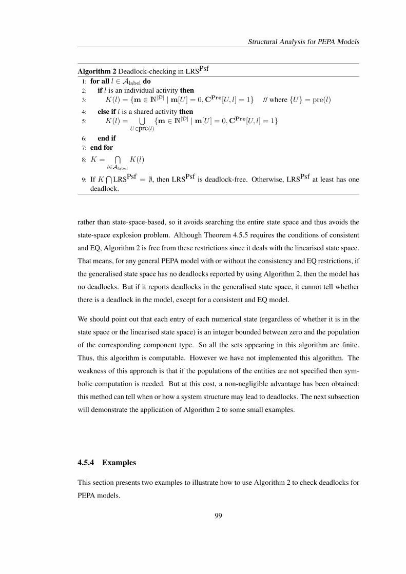
Structural Analysis for PEPA Models
Algorithm 2 Deadlock-checking in LRSPsf
1: for all l ∈ Alabel do2: if l is an individual activity then3: K(l) = {m ∈ N|D| | m[U ] = 0,CPre[U, l] = 1} // where {U} = pre(l)
4: else if l is a shared activity then5: K(l) =
⋃U∈pre(l)
{m ∈ N|D| | m[U ] = 0,CPre[U, l] = 1}
6: end if7: end for8: K =
⋂l∈Alabel
K(l)
9: If K⋂
LRSPsf = ∅, then LRSPsf is deadlock-free. Otherwise, LRSPsf at least has onedeadlock.
rather than state-space-based, so it avoids searching the entire state space and thus avoids the
state-space explosion problem. Although Theorem 4.5.5 requires the conditions of consistent
and EQ, Algorithm 2 is free from these restrictions since it deals with the linearised state space.
That means, for any general PEPA model with or without the consistency and EQ restrictions, if
the generalised state space has no deadlocks reported by using Algorithm 2, then the model has
no deadlocks. But if it reports deadlocks in the generalised state space, it cannot tell whether
there is a deadlock in the model, except for a consistent and EQ model.
We should point out that each entry of each numerical state (regardless of whether it is in the
state space or the linearised state space) is an integer bounded between zero and the population
of the corresponding component type. So all the sets appearing in this algorithm are finite.
Thus, this algorithm is computable. However we have not implemented this algorithm. The
weakness of this approach is that if the populations of the entities are not specified then sym-
bolic computation is needed. But at this cost, a non-negligible advantage has been obtained:
this method can tell when or how a system structure may lead to deadlocks. The next subsection
will demonstrate the application of Algorithm 2 to some small examples.
4.5.4 Examples
This section presents two examples to illustrate how to use Algorithm 2 to check deadlocks for
PEPA models.
99
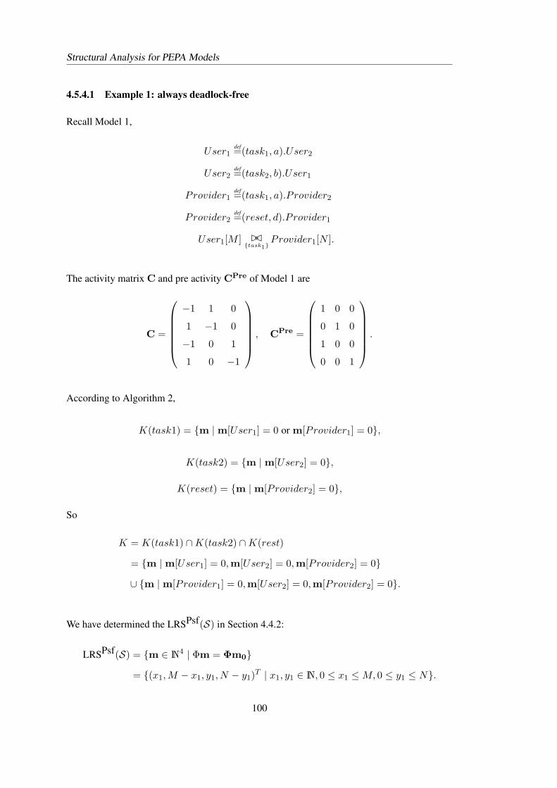
Structural Analysis for PEPA Models
4.5.4.1 Example 1: always deadlock-free
Recall Model 1,
User1def=(task1, a).User2
User2def=(task2, b).User1
Provider1def=(task1, a).P rovider2
Provider2def=(reset, d).P rovider1
User1[M ] BC{task1}
Provider1[N ].
The activity matrix C and pre activity CPre of Model 1 are
C =
−1 1 0
1 −1 0
−1 0 1
1 0 −1
, CPre =
1 0 0
0 1 0
1 0 0
0 0 1
.
According to Algorithm 2,
K(task1) = {m | m[User1] = 0 or m[Provider1] = 0},
K(task2) = {m | m[User2] = 0},
K(reset) = {m | m[Provider2] = 0},
So
K = K(task1) ∩K(task2) ∩K(rest)
= {m | m[User1] = 0,m[User2] = 0,m[Provider2] = 0}
∪ {m | m[Provider1] = 0,m[User2] = 0,m[Provider2] = 0}.
We have determined the LRSPsf(S) in Section 4.4.2:
LRSPsf(S) = {m ∈ N4 | Φm = Φm0}
= {(x1,M − x1, y1, N − y1)T | x1, y1 ∈ N, 0 ≤ x1 ≤ M, 0 ≤ y1 ≤ N}.
100
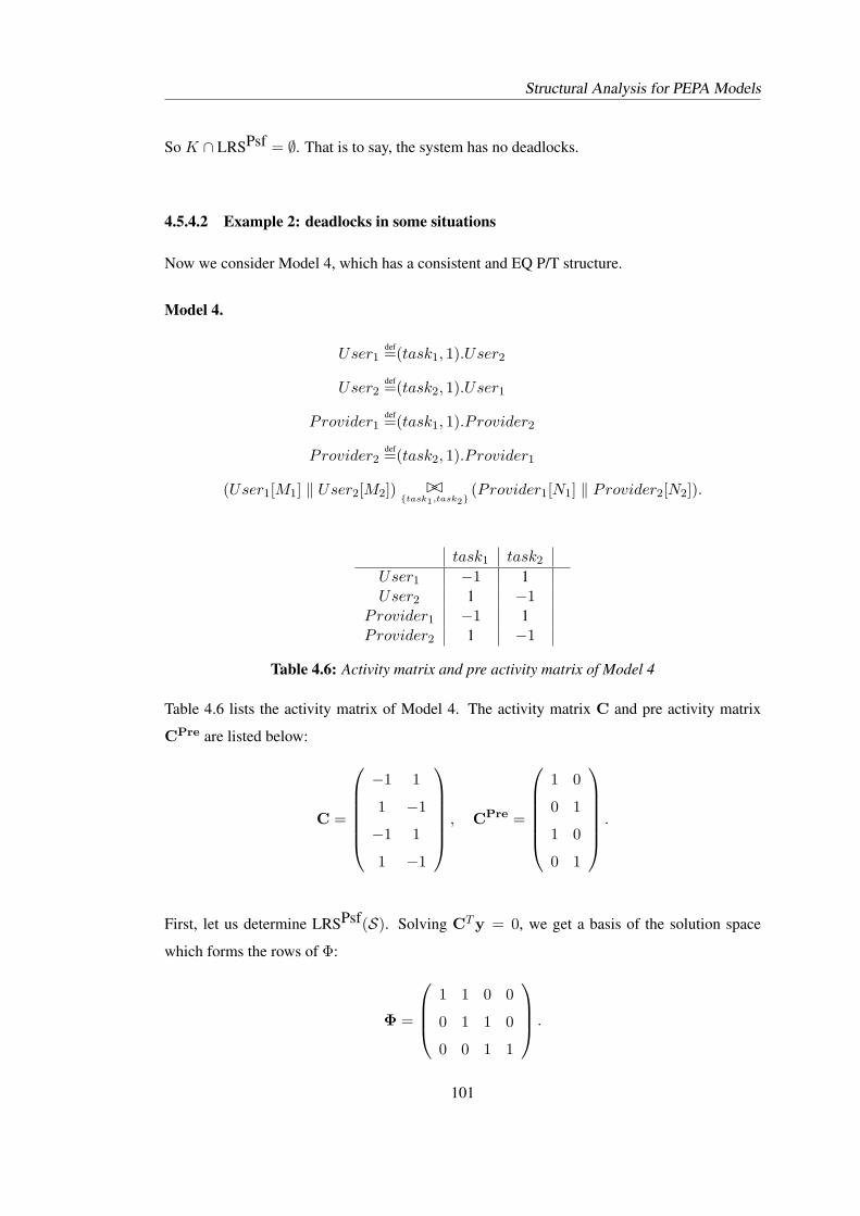
Structural Analysis for PEPA Models
So K ∩ LRSPsf = ∅. That is to say, the system has no deadlocks.
4.5.4.2 Example 2: deadlocks in some situations
Now we consider Model 4, which has a consistent and EQ P/T structure.
Model 4.
User1def=(task1, 1).User2
User2def=(task2, 1).User1
Provider1def=(task1, 1).P rovider2
Provider2def=(task2, 1).P rovider1
(User1[M1] ‖ User2[M2]) BC{task1,task2}
(Provider1[N1] ‖ Provider2[N2]).
task1 task2
User1 −1 1User2 1 −1
Provider1 −1 1Provider2 1 −1
Table 4.6: Activity matrix and pre activity matrix of Model 4
Table 4.6 lists the activity matrix of Model 4. The activity matrix C and pre activity matrix
CPre are listed below:
C =
−1 1
1 −1
−1 1
1 −1
, CPre =
1 0
0 1
1 0
0 1
.
First, let us determine LRSPsf(S). Solving CTy = 0, we get a basis of the solution space
which forms the rows of Φ:
Φ =
1 1 0 0
0 1 1 0
0 0 1 1
.
101
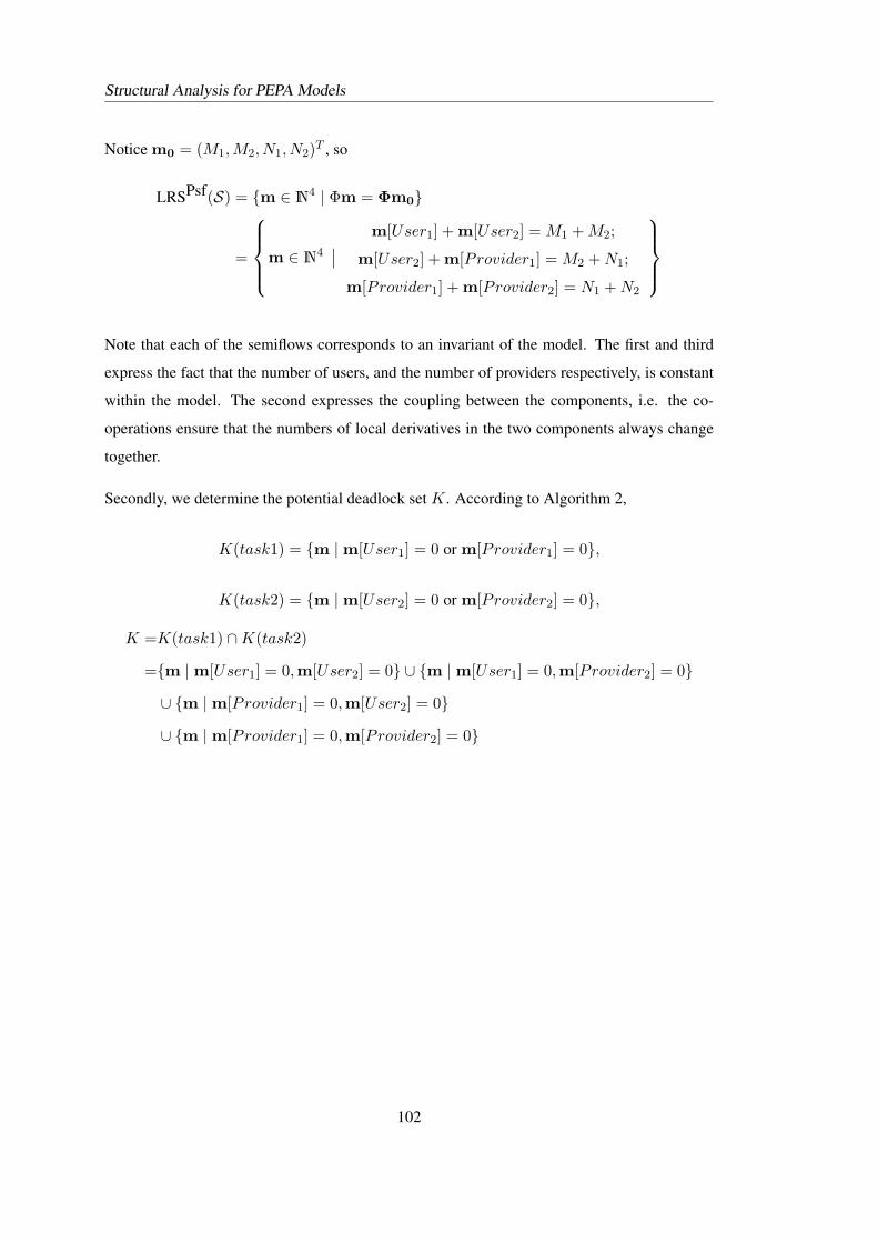
Structural Analysis for PEPA Models
Notice m0 = (M1,M2, N1, N2)T , so
LRSPsf(S) = {m ∈ N4 | Φm = Φm0}
=
m ∈ N4∣∣ m[User1] + m[User2] = M1 + M2;
m[User2] + m[Provider1] = M2 + N1;
m[Provider1] + m[Provider2] = N1 + N2
Note that each of the semiflows corresponds to an invariant of the model. The first and third
express the fact that the number of users, and the number of providers respectively, is constant
within the model. The second expresses the coupling between the components, i.e. the co-
operations ensure that the numbers of local derivatives in the two components always change
together.
Secondly, we determine the potential deadlock set K. According to Algorithm 2,
K(task1) = {m | m[User1] = 0 or m[Provider1] = 0},
K(task2) = {m | m[User2] = 0 or m[Provider2] = 0},
K =K(task1) ∩K(task2)
={m | m[User1] = 0,m[User2] = 0} ∪ {m | m[User1] = 0,m[Provider2] = 0}
∪ {m | m[Provider1] = 0,m[User2] = 0}
∪ {m | m[Provider1] = 0,m[Provider2] = 0}
102
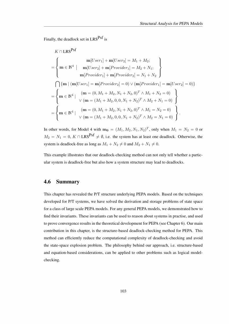
Structural Analysis for PEPA Models
Finally, the deadlock set in LRSPsf is
K ∩ LRSPsf
=
m ∈ N4∣∣ m[User1] + m[User2] = M1 + M2;
m[User2] + m[Provider1] = M2 + N1;
m[Provider1] + m[Provider2] = N1 + N2
⋂{m | (m[User1] = m[Provider2] = 0) ∨ (m[Provider1] = m[User2] = 0)}
=
m ∈ N4 |(m = (0,M1 + M2, N1 + N2, 0)T ∧M1 + N2 = 0)
∨ (m = (M1 + M2, 0, 0, N1 + N2)T ∧M2 + N1 = 0)
=
m ∈ N4 |(m = (0,M1 + M2, N1 + N2, 0)T ∧M1 = N2 = 0)
∨ (m = (M1 + M2, 0, 0, N1 + N2)T ∧M2 = N1 = 0)
.
In other words, for Model 4 with m0 = (M1,M2, N1, N2)T , only when M1 = N2 = 0 or
M2 = N1 = 0, K ∩ LRSPsf 6= ∅, i.e. the system has at least one deadlock. Otherwise, the
system is deadlock-free as long as M1 + N2 6= 0 and M2 + N1 6= 0.
This example illustrates that our deadlock-checking method can not only tell whether a partic-
ular system is deadlock-free but also how a system structure may lead to deadlocks.
4.6 Summary
This chapter has revealed the P/T structure underlying PEPA models. Based on the techniques
developed for P/T systems, we have solved the derivation and storage problems of state space
for a class of large scale PEPA models. For any general PEPA models, we demonstrated how to
find their invariants. These invariants can be used to reason about systems in practise, and used
to prove convergence results in the theoretical development for PEPA (see Chapter 6). Our main
contribution in this chapter, is the structure-based deadlock-checking method for PEPA. This
method can efficiently reduce the computational complexity of deadlock-checking and avoid
the state-space explosion problem. The philosophy behind our approach, i.e. structure-based
and equation-based considerations, can be applied to other problems such as logical model-
checking.
103

104
Chapter 5Fluid Analysis for Large Scale PEPA
Models—Part I: ProbabilisticApproach
5.1 Introduction
In the previous chapter we have discussed the techniques of structural analysis for large scale
PEPA models, to deal with the state-space explosion problem. Quantitative analysis of large
scale PEPA models also suffers from this problem, which is encountered in the calculation
of steady-state probability distributions of the CTMCs. The state-space explosion problem
is inherent in the discrete state approach employed in stochastic process algebras and many
other formal modelling approaches. Recently, for the stochastic process algebra PEPA [Hil96],
Hillston has developed a novel approach—continuous state-space approximation—to avoid this
problem [Hil05a]. This approach results in a set of ODEs, leading to the evaluation of transient
and, in the limit, steady state measures.
More recently, an extension of the previous mapping from PEPA to ODEs, relaxing some
structure restrictions, has been presented in [BGH07]. In particular, synchronisations are al-
lowed between active and passive actions. The relationship between the derived ODEs and the
CTMCs for a special example in the context of PEPA, was revealed in [GHS08]: the set of
ODEs automatically extracted from the PEPA description are the limits of the sequence of un-
derlying CTMCs. However, for general applications the structure restrictions in both [BGH07]
and [GHS08] should be further relaxed. For example, an individual activity may occur more
than once within derivative definitions and can appear within different component definitions.
Moreover, shared activities may have different local rates in realistic scenarios.
In this chapter, we relax these conditions and extend the mapping semantics, by employing
the activity matrices and transition rate functions introduced in Chapter 3. Moreover, we will
establish some fundamental characteristics of the solutions of the derived ODEs, such as the
105
Fluid Analysis for Large Scale PEPA Models—Part I: Probabilistic Approach
existence, uniqueness and convergence. For PEPA models without synchronisations, we will
show that the solutions of the derived ODEs have finite limits and the limits coincide with
the steady-state probability distributions of the underlying CTMCs. For general PEPA models
with synchronisations, based on the pioneering work in [GHS08], the consistency between the
derived ODEs and a family of underlying density dependent CTMCs has been demonstrated.
Furthermore, we will show the convergence of the solutions of the ODEs generated from gen-
eral PEPA models under a particular condition.
We assume in this chapter that the CTMCs underlying considered PEPA models are irreducible
and positive-recurrent [And91]. By Theorem 3.5.3 in [Hil96], the CTMC underlying a PEPA
model is irreducible if and only if the initial component of the model is cyclic. According
to the conclusion (Proposition 1.7, page 163, [And91]) that an irreducible Markov chain is
positive-recurrent if and only if there exists a steady-state distribution, it is natural to assume
the underlying CTMCs to be positive-recurrent because some discussions in the following are
based on the existence of steady-state distributions. Under the assumption of these two condi-
tions, i.e. irreducible and positive-recurrent, the CTMCs underlying considered PEPA models
have steady-state probability distributions, which has also been illustrated in Theorem 3.5.2
in [Hil96].
The remainder of this chapter is structured as follows. Section 2 describes the fluid approxima-
tions of general PEPA models, as well as the existence and uniqueness theorem for the derived
ODEs, while the convergence of the solutions in the nonsynchronisation case is presented in
Section 3. Section 4 presents the concept of density dependent CTMCs and the relationship be-
tween this concept and the derived ODEs, based on which the convergence of the ODE solutions
under a particular condition for general PEPA models will be shown in Section 5. Section 6
presents the further investigation of this particular condition. Finally, we conclude the chapter
in Section 7.
5.2 Fluid Approximations for PEPA Models
The section will introduce the fluid-flow approximations for PEPA models, which leads to some
kind of nonlinear ODEs. The existence and uniqueness of the solutions of the ODEs will be
established. Moreover, a conservation law satisfied by the ODEs will be shown.
106
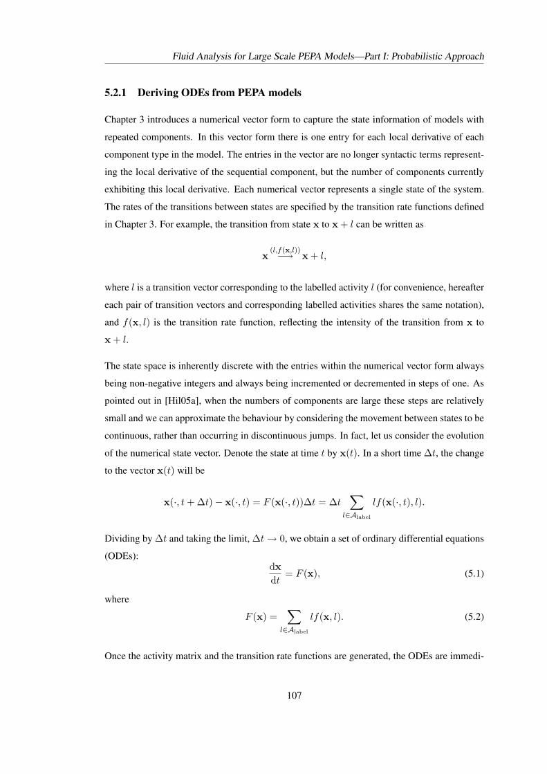
Fluid Analysis for Large Scale PEPA Models—Part I: Probabilistic Approach
5.2.1 Deriving ODEs from PEPA models
Chapter 3 introduces a numerical vector form to capture the state information of models with
repeated components. In this vector form there is one entry for each local derivative of each
component type in the model. The entries in the vector are no longer syntactic terms represent-
ing the local derivative of the sequential component, but the number of components currently
exhibiting this local derivative. Each numerical vector represents a single state of the system.
The rates of the transitions between states are specified by the transition rate functions defined
in Chapter 3. For example, the transition from state x to x + l can be written as
x(l,f(x,l))−→ x + l,
where l is a transition vector corresponding to the labelled activity l (for convenience, hereafter
each pair of transition vectors and corresponding labelled activities shares the same notation),
and f(x, l) is the transition rate function, reflecting the intensity of the transition from x to
x + l.
The state space is inherently discrete with the entries within the numerical vector form always
being non-negative integers and always being incremented or decremented in steps of one. As
pointed out in [Hil05a], when the numbers of components are large these steps are relatively
small and we can approximate the behaviour by considering the movement between states to be
continuous, rather than occurring in discontinuous jumps. In fact, let us consider the evolution
of the numerical state vector. Denote the state at time t by x(t). In a short time ∆t, the change
to the vector x(t) will be
x(·, t + ∆t)− x(·, t) = F (x(·, t))∆t = ∆t∑
l∈Alabel
lf(x(·, t), l).
Dividing by ∆t and taking the limit, ∆t → 0, we obtain a set of ordinary differential equations
(ODEs):dxdt
= F (x), (5.1)
where
F (x) =∑
l∈Alabel
lf(x, l). (5.2)
Once the activity matrix and the transition rate functions are generated, the ODEs are immedi-
107
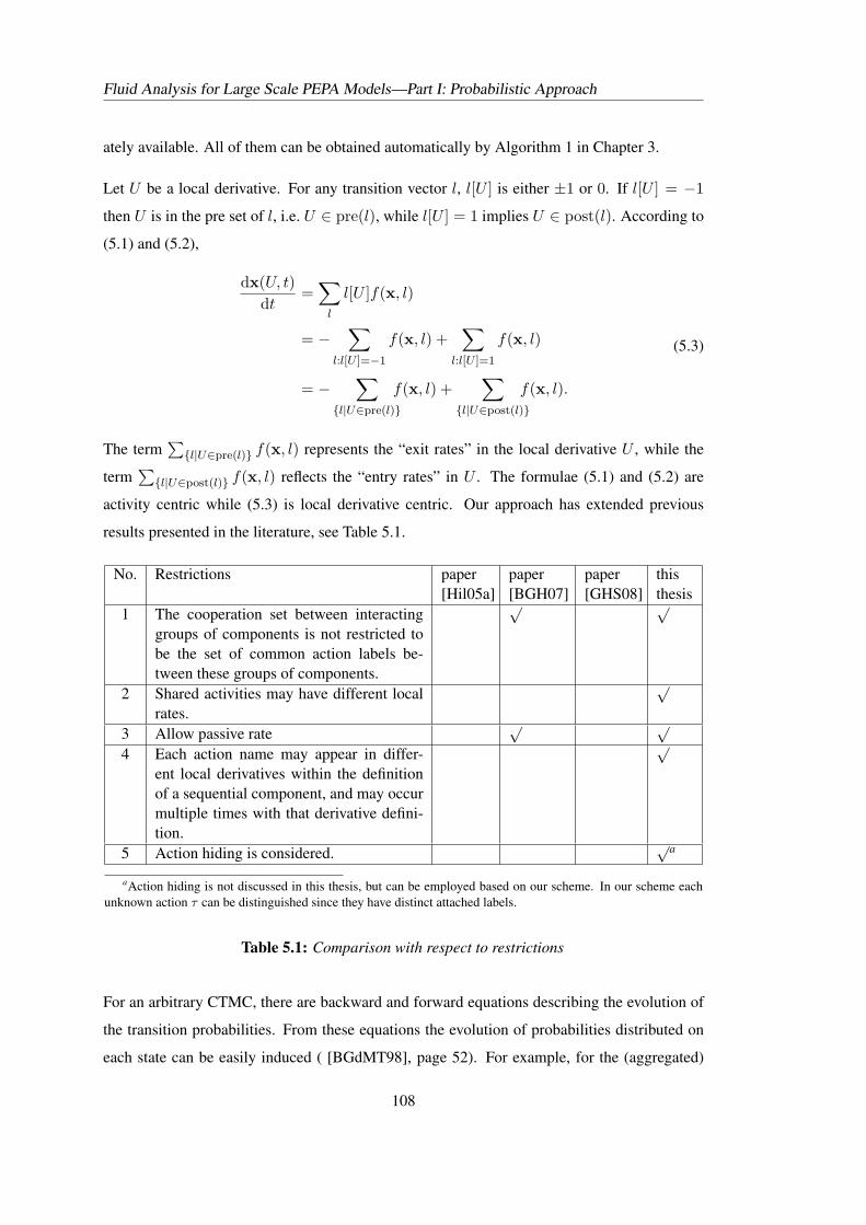
Fluid Analysis for Large Scale PEPA Models—Part I: Probabilistic Approach
ately available. All of them can be obtained automatically by Algorithm 1 in Chapter 3.
Let U be a local derivative. For any transition vector l, l[U ] is either ±1 or 0. If l[U ] = −1
then U is in the pre set of l, i.e. U ∈ pre(l), while l[U ] = 1 implies U ∈ post(l). According to
(5.1) and (5.2),
dx(U, t)dt
=∑
l
l[U ]f(x, l)
= −∑
l:l[U ]=−1
f(x, l) +∑
l:l[U ]=1
f(x, l)
= −∑
{l|U∈pre(l)}
f(x, l) +∑
{l|U∈post(l)}
f(x, l).
(5.3)
The term∑
{l|U∈pre(l)} f(x, l) represents the “exit rates” in the local derivative U , while the
term∑
{l|U∈post(l)} f(x, l) reflects the “entry rates” in U . The formulae (5.1) and (5.2) are
activity centric while (5.3) is local derivative centric. Our approach has extended previous
results presented in the literature, see Table 5.1.
No. Restrictions paper[Hil05a]
paper[BGH07]
paper[GHS08]
thisthesis
1 The cooperation set between interactinggroups of components is not restricted tobe the set of common action labels be-tween these groups of components.
√ √
2 Shared activities may have different localrates.
√
3 Allow passive rate√ √
4 Each action name may appear in differ-ent local derivatives within the definitionof a sequential component, and may occurmultiple times with that derivative defini-tion.
√
5 Action hiding is considered.√a
aAction hiding is not discussed in this thesis, but can be employed based on our scheme. In our scheme eachunknown action τ can be distinguished since they have distinct attached labels.
Table 5.1: Comparison with respect to restrictions
For an arbitrary CTMC, there are backward and forward equations describing the evolution of
the transition probabilities. From these equations the evolution of probabilities distributed on
each state can be easily induced ( [BGdMT98], page 52). For example, for the (aggregated)
108
Fluid Analysis for Large Scale PEPA Models—Part I: Probabilistic Approach
CTMC underlying a PEPA model, the corresponding differential equations describing the evo-
lution of the probability distributions are
dπ
dt= QT π, (5.4)
where each entry of π(t) represents the probability of the system being in each state at time t,
and Q is an infinitesimal generator matrix corresponding to the CTMC. Obviously, the dimen-
sion of the coefficient matrix Q is the square of the size of the state space, which increases as
the number of components increases.
The derived ODEs (5.1) describe the evolution of the population of the components in each
local derivative, while (5.4) reflects the the probability evolution at each state. Since the scale
of (5.1), i.e. the number of the ODEs, is only determined by the number of local derivatives
and is unaffected by the size of the state space, so it avoids the state-space explosion problem.
But the scale of (5.4) depends on the size of the state space, so it suffers from the explosion
problem. The price paid is that the ODEs (5.1) are generally nonlinear due to synchronisations,
while (5.4) is linear. However, if there is no synchronisation contained then (5.1) becomes
linear, and there is some correspondence and consistency between these two different types of
ODEs, which will be demonstrated in Section 5.3.
It is well known that for an irreducible and positive-recurrent CTMC, the solution of the corre-
sponding ODEs (5.4) has a unique limit, which is the unique steady-state probability distribu-
tion of the given CTMC. From this distribution, the performance measures such as throughput
and utilisation can be derived. Analogously, we want to know whether the solution of (5.1) has
a finite limit, from which similar performance measures can also be derived. If the limit exists,
what is the relationship between the limit and the steady-state probability distribution of the
underlying CTMC? These problems are the main topics of this chapter.
109
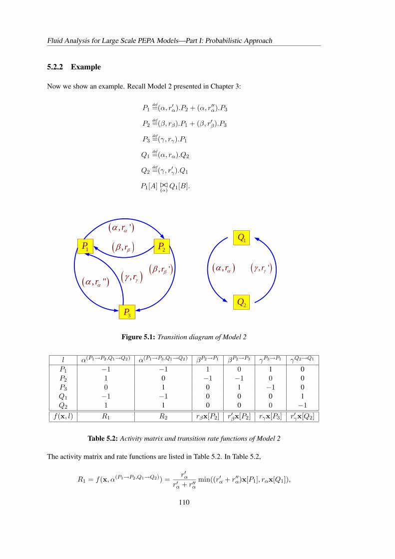
Fluid Analysis for Large Scale PEPA Models—Part I: Probabilistic Approach
5.2.2 Example
Now we show an example. Recall Model 2 presented in Chapter 3:
P1def=(α, r′α).P2 + (α, r′′α).P3
P2def=(β, rβ).P1 + (β, r′β).P3
P3def=(γ, rγ).P1
Q1def=(α, rα).Q2
Q2def=(γ, r′γ).Q1
P1[A] BC{α}
Q1[B].
( ), rαα
1Q
2Q
1P 2P
3P
( ), 'rγγ
( ), 'rαα
( ), "rαα ( ), rγγ
( ), rββ
( ), 'rββ
Figure 5.1: Transition diagram of Model 2
l α(P1→P2,Q1→Q2) α(P1→P3,Q1→Q2) βP2→P1 βP2→P3 γP3→P1 γQ2→Q1
P1 −1 −1 1 0 1 0P2 1 0 −1 −1 0 0P3 0 1 0 1 −1 0Q1 −1 −1 0 0 0 1Q2 1 1 0 0 0 −1
f(x, l) R1 R2 rβx[P2] r′βx[P2] rγx[P3] r′γx[Q2]
Table 5.2: Activity matrix and transition rate functions of Model 2
The activity matrix and rate functions are listed in Table 5.2. In Table 5.2,
R1 = f(x, α(P1→P2,Q1→Q2)) =r′α
r′α + r′′αmin((r′α + r′′α)x[P1], rαx[Q1]),
110
Fluid Analysis for Large Scale PEPA Models—Part I: Probabilistic Approach
R2 = f(x, α(P1→P3,Q1→Q2)) =r′′α
r′α + r′′αmin((r′α + r′′α)x[P1], rαx[Q1]).
According to our approach, the derived ODEs are
(dx(P1)
dt,dx(P2)
dt,dx(P3)
dt,dx(Q1)
dt,dx(Q2)
dt
)T
=∑
l
lf(x, l)
= f(x, α(P1→P2,Q1→Q2))
−1
1
0
−1
1
+ f(x, α(P1→P3,Q1→Q2))
−1
0
1
0
1
+ rβx(P2)
1
−1
0
0
0
+ r′βx(P2)
0
−1
1
0
0
+ rγx(P3)
1
0
−1
0
0
+ r′γx(Q2)
0
0
0
1
−1
,
that is
dx(P1)dt = −min((r′α + r′′α)x(P1), rαx(Q1)) + r′βx(P2)) + rγx(P3)
dx(P2)dt = r′α
r′α+r′′αmin((r′α + r′′α)x(P1), rαx(Q1))− (rβ + r′β)x(P2)
dx(P3)dt = r′′α
r′α+r′′αmin((r′α + r′′α)x(P1), rαx(Q1)) + rβx(P2)− rγx(P3)
dx(Q1)dt = −min((r′α + r′′α)x(P1), rαx(Q1)) + r′γx(Q2)
dx(Q2)dt = min((r′α + r′′α)x(P1), rαx(Q1))− r′γx(Q2)
.
Hereafter the notation x[·] indicates a discrete state x, while x(·) or x(·, t) reflects a continuous
state x at time t.
Notice that in the PEPA language the passive rate “>” is in fact a notation rather than a number.
Since 0 · > = 0 is assumed in Chapter 3 (see Remark 3.4.1), in the above ODEs the terms such
as “min{A>, rB}” are therefore interpreted as [BGH07]:
min{A>, rB} =
rB, A > 0,
0, A = 0.
111
Fluid Analysis for Large Scale PEPA Models—Part I: Probabilistic Approach
For example, if rα is a passive rate, i.e. rα = >, then the derived ODEs are as
dx(P1)dt = −min((r′α + r′′α)x(P1),x(Q1)>) + r′βx(P2) + rγx(P3)
dx(P2)dt = r′α
r′α+r′′αmin((r′α + r′′α)x(P1),x(Q1)>)− (rβ + r′β)x(P2)
dx(P3)dt = r′′α
r′α+r′′αmin((r′α + r′′α)x(P1),x(Q1)>) + rβx(P2)− rγx(P3)
dx(Q1)dt = −min((r′α + r′′α)x(P1),x(Q1)>) + r′γx(Q2)
dx(Q2)dt = min((r′α + r′′α)x(P1),x(Q1)>)− r′γx(Q2)
.
Introducing the passive rate into ODEs is first considered in [BGH07] and [Hay07b]. We should
point out that the above definition of “min{A>, rB}” may result in jumps in the functions on
the right side of the ODEs. Then, by the theory of ordinary differential equations, these ODEs
may have no solutions. In this case, in order to guarantee the existence of solutions, these
ODEs should be interpreted as difference rather than differential equations, or considered as
integration equations.
In the remainder of this thesis, unless otherwise stated there are no passive rates involved in the
derived ODEs. As we will show in the following subsection, if there are no passive rates, then
the derived ODEs must have solutions in the time interval [0,∞).
5.2.3 Existence and uniqueness of ODE solution
For any set of ODEs, it is important to consider if the equations have a solution, and if so
whether that solution is unique.
Theorem 5.2.1. For a given PEPA model without passive rates, the derived ODEs from this
model have a unique solution in the time interval [0,∞).
Proof. Notice that each entry of F (x) =∑
l lf(x, l) is a linear combination of the rate func-
tions f(x, l), so F (x) is Lipschitz continuous since each f(x, l) is Lipschitz continuous by
Proposition 3.4.3 in Chapter 3. That is, there exits M > 0 such that ∀x,y,
||F (x)− F (y)|| ≤ M ||x− y||. (5.5)
By Theorem C.1.1 in Appendix C.1, the derived ODEs have a unique solution in [0,∞).
In the remainder of this subsection, we introduce a proposition, which states that the ODEs
112
Fluid Analysis for Large Scale PEPA Models—Part I: Probabilistic Approach
derived from PEPA models satisfy a conservation law. As we have mentioned, in the formula
dx(U, t)dt
= −∑
{l|U∈pre(l)}
f(x, l) +∑
{l|U∈post(l)}
f(x, l),
the term∑
{l|U∈pre(l)} f(x, l) represents the exit rates in the local derivative U , while the term∑{l|U∈post(l)} f(x, l) reflects the entry rates in U . For each type of component at any time,
the sum of all exit activity rates must be equal to the sum of all entry activity rates, since the
system is closed and there is no exchange with the environment. This leads to the following
proposition.
Proposition 5.2.1. Let Cij be a local derivative of component type Ci. Then for any i and t,∑j
dx(Cij , t
)dt
= 0, and∑
j x(Cij , t
)=∑
j x(Cij , 0
).
Proof. We have mentioned in Chapter 3 that the numbers of −1 and 1 appearing in the entries
of any transition vector l, which correspond to the component type Ci, are the same, i.e.
#{j : l[Cij ] = −1} = #{j : l[Cij ] = 1}. (5.6)
Let y be an indicator vector with the same dimension as l satisfying:
y[Cij ] =
1, if l[Cij ] = ±1,
0, otherwise.
So yT l = 0 by (5.6). Thus
yT dxdt
= yT∑
l
lf(x, l) =∑
l
yT lf(x, l) = 0.
That is,∑
j
dx(Cij , t
)dt
= yT dxdt
= 0. So∑
j x(Cij , t
)is a constant and equal to
∑j x(Cij , 0
),
i.e. the number of the copies of component type Ci in the system initially.
Proposition 5.2.1 means that the ODEs satisfy a Conservation Law, i.e. the number of each
kind of component remains constant at all times.
113
Fluid Analysis for Large Scale PEPA Models—Part I: Probabilistic Approach
5.3 Convergence of ODE Solution: without Synchronisations
Now we consider PEPA models without synchronisation. For this special class of PEPA models,
we will show that the solutions of the derived ODEs have finite limits. Moreover, the limits
coincide with the steady-state probability distributions of the underlying CTMCs.
5.3.1 Features of ODEs without synchronisations
Suppose the PEPA model has no synchronisation. Without loss of generality, we suppose that
there is only one kind of component C in the system. In fact, if there are several types of
component in the system, the ODEs related to the different types of component can be separated
and treated independently since there are no interactions between them. Thus, we assume there
is only one kind of component C and that C has k local derivatives: C1, C2, · · · , Ck. Then
(5.1) is
d (x(C1, t), · · · ,x(Ck, t))T
dt=∑
l
lf(x, l). (5.7)
Since (5.7) are linear ODEs, we may rewrite (5.7) as the following matrix form:
d (x(C1, t), · · · ,x(Ck, t))T
dt= QT (x(C1, t), · · · ,x(Ck, t))
T , (5.8)
where Q = (qij) is a k × k matrix.
Q has many good properties.
Proposition 5.3.1. Q = (qij)k×k in (5.8) is an infinitesimal generator matrix, that is, (qij)k×k
satisfies
1. 0 ≤ −qii < ∞ for all i;
2. qij ≥ 0 for all i 6= j;
3.∑k
j=1 qij = 0 for all i.
Proof. According to (5.8), we have
dx(Ci, t)dt
=k∑
j=1
x(Cj , t)qji. (5.9)
114
Fluid Analysis for Large Scale PEPA Models—Part I: Probabilistic Approach
Notice by (5.3),
dx(Ci, t)dt
= −∑
{l|Ci∈pre(l)}
f(x, l) +∑
{l|Ci∈post(l)}
f(x, l).
Sok∑
j=1
x(Cj , t)qji = −∑
{l|Ci∈pre(l)}
f(x, l) +∑
{l|Ci∈post(l)}
f(x, l). (5.10)
Since there is no synchronisation in the system, the transition function f(x, l) is linear with
respect to x and there is no nonlinear term ,“min”, in it. In particular, if Ci ∈ pre(l), then
f(x, l) = r(Ci)lx[Ci], which is the apparent rate of l in Ci in state x defined in Definition 3.4.1
in Chapter 3. We should point out that according to our semantics of mapping PEPA models to
ODEs, the fluid approximation-version of f(x, l) also holds, i.e. f(x(t), l) = rl(Ci)x(Ci, t).
So (5.10) becomes
x(Ci, t)qii +∑j 6=i
x(Cj , t)qji = x(Ci, t)∑
{l|Ci∈pre(l)}
(−rl(Ci)) +∑
{l|Ci∈post(l)}
f(x, l). (5.11)
Moreover, as long as f(x, l) = rl(Ci)x(Ci) for some l and some positive constants rl(Ci),
which implies that l can be fired at Ci, we must have Ci ∈ pre(l). That is to say, if Ci ∈ post(l)
then f(x, l) cannot be of the form of rx(Ci, t) for any constant r > 0. Otherwise, we have
Ci ∈ pre(l), which results a contradiction1 to Ci ∈ post(l). So according to (5.11), we have
x(Ci, t)qii = x(Ci, t)∑
{l|Ci∈pre(l)}
(−rl(Ci)) , (5.12)
∑j 6=i
x(Cj , t)qji =∑
{l|Ci∈post(l)}
f(x, l). (5.13)
Thus by (5.12), qii =∑
{l|Ci∈pre(l)} (−rl(Ci)), and 0 ≤ −qii < ∞ for all i. Item 1 is proved.
Similarly, for any Cj , j 6= i, if f(x, l) = rx(Cj , t) for some l and positive constant r, then
obviously Cj is in the pre set of l. That is Cj ∈ pre(l). So by (5.13),
x(Cj , t)qji =∑
{l|Cj∈pre(l),Ci∈post(l)}
f(x, l) = x(Cj , t)∑
l
rCj→Ci
l , (5.14)
1In this chapter we do not allow a self-loop in the considered model. That is, any PEPA definition like
“Cdef= (α, r).C” which results in C ∈ pre(α) and C ∈ post(α) simultaneously, is not allowed.
115
Fluid Analysis for Large Scale PEPA Models—Part I: Probabilistic Approach
which implies qji =∑
l rCj→Ci
l ≥ 0 for all i 6= j, i.e. item 2 holds.
We now prove item 3. By Proposition 5.2.1,
x(C1, t)dt
+x(C2, t)
dt+ · · ·+ x(Ck, t)
dt= 0. (5.15)
Then by (5.9) and (5.15), for all t,
x(C1, t)k∑
j=1
q1j + x(C2, t)k∑
j=1
q2j + · · ·+ x(Ck, t)k∑
j=1
qkj
=k∑
i=1
x(Ci, t)k∑
j=1
qij
=k∑
j=1
k∑i=1
x(Ci, t)qij
=k∑
j=1
dx(Cj , t)dt
=0.
This implies∑k
j=1 qij = 0 for all i.
We point out that this infinitesimal generator matrix Qk×k may not be the infinitesimal gen-
erator matrix of the CTMC derived via the usual semantics of PEPA (we call it the “original”
CTMC for convenience). In fact, the original CTMC has a state space with kN states and the
dimension of its infinitesimal generator matrix is kN×kN , where N is the total number of com-
ponents in the system. However, this Qk×k is the infinitesimal generator matrix of a CTMC
underlying the PEPA model in which there is only one copy of the component, i.e. N = 1. To
distinguish this from the original one, we refer to this CTMC as the “singleton” CTMC.
In the proof of Proposition 5.3.1, we have shown the relationship between the coefficient matrix
Q and the activity rates:
qii = −∑
{l|Ci∈pre(l)}
rl(Ci), qij =∑
l
rCi→Cj
l (i 6= j).
We use an example to illustrate the above equalities:
116
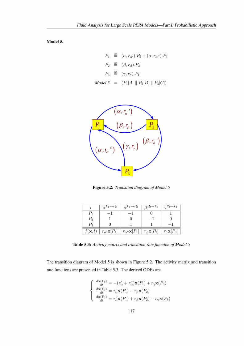
Fluid Analysis for Large Scale PEPA Models—Part I: Probabilistic Approach
Model 5.
P1def= (α, rα′).P2 + (α, rα′′).P3
P2def= (β, rβ).P3
P3def= (γ, rγ).P1
Model 5 = (P1[A] ‖ P2[B] ‖ P3[C])
1P 2P
3P
( ), 'rαα
( ), "rαα ( ), rγγ
( ), rββ
( ), 'rββ
Figure 5.2: Transition diagram of Model 5
l αP1→P2 αP1→P3 βP2→P3 γP3→P1
P1 −1 −1 0 1P2 1 0 −1 0P3 0 1 1 −1
f(x, l) rα′x[P1] rα′′x[P1] rβx[P2] rγx[P3]
Table 5.3: Activity matrix and transition rate function of Model 5
The transition diagram of Model 5 is shown in Figure 5.2. The activity matrix and transition
rate functions are presented in Table 5.3. The derived ODEs are
dx(P1)
dt = −(r′α + r′′α)x(P1) + rγx(P3)dx(P2)
dt = r′αx(P1)− rβx(P2)dx(P3)
dt = r′′αx(P1) + rβx(P2)− rγx(P3)
117
Fluid Analysis for Large Scale PEPA Models—Part I: Probabilistic Approach
or dx(P1)
dtdx(P2)
dtdx(P3)
dt
=
−(rα′ + rα′′) 0 rγ
rα′ −rβ 0
rα′′ rβ −rγ
x(P1)
x(P2)
x(P3)
= QT
x(P1)
x(P2)
x(P3)
,
where
Q =
−(rα′ + rα′′) rα′ rα′′
0 −rβ rβ
rγ 0 −rγ
is clearly an infinitesimal generator matrix. Obviously, q11 = −(rα′+rα′′) = −
∑{l|P1∈pre(l)}
rl(P1).
Similarly, qij =∑
l rPi→Pj
l (i 6= j).
5.3.2 Convergence and consistency for the ODEs
Proposition 5.3.1 illustrates that the coefficient matrix of the derived ODEs is an infinitesimal
generator. If there is only one component in the system, then equation (5.8) captures the proba-
bility distribution evolution equations of the original CTMC. Based on this proposition, we can
furthermore determine the convergence of the solutions.
Theorem 5.3.1. Suppose x (Cj , t) (j = 1, 2, · · · , k) satisfy (5.7), then for any given initial
values x (Cj , 0) ≥ 0 (j = 1, 2, · · · , k), there exist constants x(Cj ,∞), such that
limt→∞
x(Cj , t) = x(Cj ,∞), j = 1, 2, · · · , k. (5.16)
Proof. By Proposition 5.3.1, the matrix Q in (5.8) is an infinitesimal generator matrix. Con-
sider a “singleton” CTMC which has the state space S = {C1, C2, · · · , Ck}, the infinitesimal
generator matrix Q in (5.8) and the initial probability distribution π(Cj , 0) = x(Cj ,0)N (j =
1, 2, · · · , k). Then according to Markov theory ( [BGdMT98], page 52), π(Cj , t) (j = 1, 2, · · · , k),
the probability distribution of this new CTMC at time t, satisfies
d (π(C1, t), · · · , π(Ck, t))dt
= (π(C1, t), · · · , π(Ck, t))Q (5.17)
Since the singleton CTMC is assumed irreducible and positive-recurrent, it has a steady-state
118
Fluid Analysis for Large Scale PEPA Models—Part I: Probabilistic Approach
probability distribution {π(Cj ,∞)}kj=1, and
limt→∞
π(Cj , t) = π(Cj ,∞), j = 1, 2, · · · , k. (5.18)
Note that x(Cj ,t)N also satisfies (5.17) with the initial values x(Cj ,0)
N equal to π(Cj , 0), where N
is the population of the components. By the uniqueness of the solutions of (5.17), we have
x(Cj , t)N
= π(Cj , t), j = 1, 2, · · · , k, (5.19)
and hence by (5.18),
limt→∞
x(Cj , t) = limt→∞
Nπ(Cj , t) = Nπ(Cj ,∞), j = 1, 2, · · · , k.
Remark 5.3.1. Suppose there are m types of components in the system: C1, C2, · · · , Cm, each
with k1, k2, · · · , km local derivatives respectively. Since there is no cooperation between dif-
ferent types of component, we can deal with each type independently. Thus, by Theorem 5.3.1,
for each component type Ci,
limt→∞
x(Cij , t) = Niπ(Cij ,∞), j = 1, 2, · · · , ki, (5.20)
where {π(Cij )}j=1,2,··· ,kiare the corresponding steady state distributions, and Ni is the popu-
lation of Ci, i = 1, 2, · · · ,m.
It is shown in [Gil05] that for some special examples the equilibrium solutions of the ODEs
coincide with the steady state probability distributions of the underlying original CTMC. This
theorem states that this holds for all for PEPA models without synchronisations.
5.4 Relating to Density Dependent CTMCs
For a PEPA model without synchronisation, the solution of the derived ODEs through the fluid
approximation has a finite limit that is consistent with the steady-state distribution of the cor-
responding singleton CTMC, as Theorem 5.3.1 exposes. However, a general PEPA model may
have synchronisations, which result in the nonlinearity of the derived ODEs. Generally, it is
difficult to rely on pure analytical methods to explore the asymptotic behaviour of the solution
119
Fluid Analysis for Large Scale PEPA Models—Part I: Probabilistic Approach
of the derived ODEs from an arbitrary PEPA model (except for some special classes of models,
see the next chapter).
Fortunately, Kurtz’s theorem [Kur70, EK86] establishes the relationship between a sequence
of Markov chains and a corresponding set of ODEs: the complete solution of some ODEs is
the limit of a sequence of Markov chains. In the context of PEPA, the derived ODEs can be
considered as the limit of pure jump Markov processes, as first exposed in [GHS08] for a special
case. Thus we may investigate the convergence of the ODE solutions by alternatively studying
the corresponding property of the Markov chains through this consistency relationship.
This approach leads to the result presented in the next section: under a particular condition
the solution will converge and the limit is consistent with the limit steady-state probability
distribution of a family of CTMCs underlying the given PEPA model. Let us first introduce the
concept of density dependent Markov chains underlying PEPA models.
5.4.1 Density dependent Markov chains from PEPA models
In the numerical state vector representation scheme, each vector is a single state and the rates
of the transitions between states are specified by the rate functions. For example, the transition
from state s to s + l can be written as
s(l,f(s,l))−→ s + l.
Since all the transitions are only determined by the current state rather than the previous ones,
given any starting state a CTMC can be obtained. More specifically, the state space of the
CTMC is the set of all reachable numerical state vectors s. The infinitesimal generator is
determined by the transition rate function,
qs,s+l = f(s, l). (5.21)
Because the transition rate function is defined according to the semantics of PEPA, the CTMC
mentioned above is in fact the aggregated CTMC underlying the given PEPA model. In other
words, the transition rate of the aggregated CTMC is specified by the transition rate function in
Definition 3.4.2.
120
Fluid Analysis for Large Scale PEPA Models—Part I: Probabilistic Approach
It is obvious that the aggregated CTMC depends on the starting state of the given PEPA model.
By altering the population of components presented in the model, which can be done by varying
the initial states, we may get a sequence of aggregated CTMCs. Moreover, Proposition 3.4.3
indicates that the transition rate function has the homogenous property: Hf(s/H, l) = f(s, l),
∀H > 0. This property identifies the aggregated CTMC to be density dependent.
Definition 5.4.1. [Kur70]. A family of CTMCs {Xn}n is called density dependent if and
only if there exists a continuous function f(x, l), x ∈ Rd, l ∈ Zd, such that the infinitesimal
generators of Xn are given by:
q(n)s,s+l = nf(s/n, l), l 6= 0,
where q(n)s,s+l denotes an entry of the infinitesimal generator of Xn, s a numerical state vector
and l a transition vector.
This allows us to conclude the following proposition.
Proposition 5.4.1. Let {Xn} be a sequence of aggregated CTMCs generated from a given
PEPA model (by scaling the initial state), then {Xn} is density dependent.
Proof. For any n, the transition between states is determined by
q(n)s,s+l = f(s, l),
where s, s + l are state vectors, l corresponds to an activity, f(s, l) is the rate of the transition
from state s to s + l. By Proposition 3.4.3,
nf(s/n, l) = f(s, l).
So the infinitesimal generator of Xn is given by:
q(n)s,s+l = f(s, l) = nf(s/n, l), l 6= 0.
Therefore, {Xn} is a sequence of density dependent CTMCs.
In particular, the family of density dependent CTMCs, {Xn(t)}, derived from a given PEPA
model with the starting condition Xn(0) = nx0 (∀n), is called the density dependent CTMCs
121
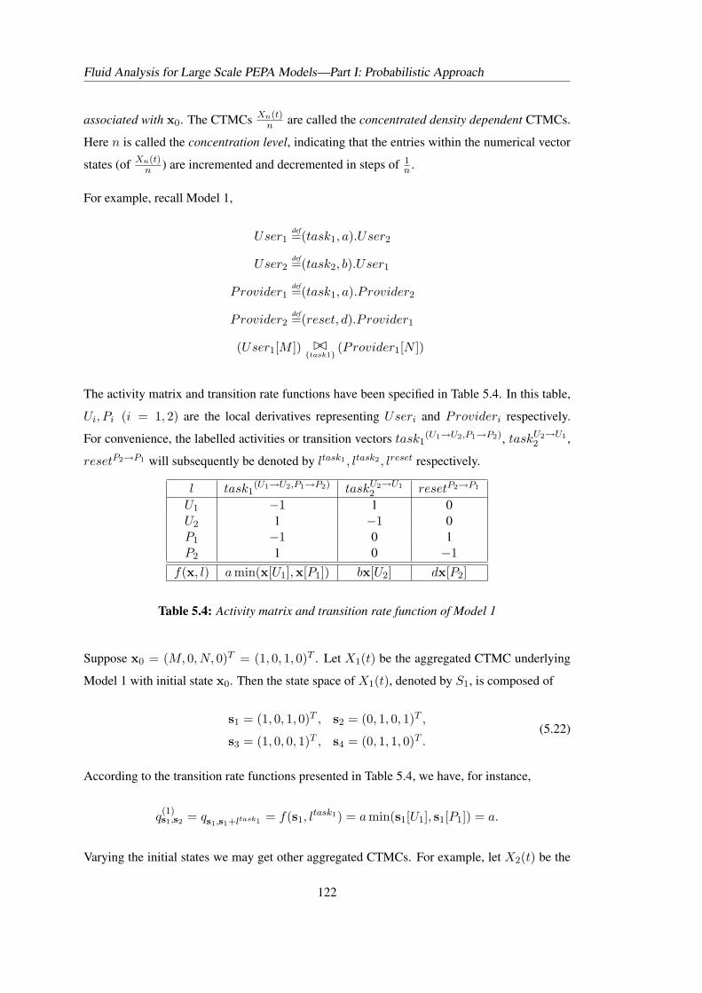
Fluid Analysis for Large Scale PEPA Models—Part I: Probabilistic Approach
associated with x0. The CTMCs Xn(t)n are called the concentrated density dependent CTMCs.
Here n is called the concentration level, indicating that the entries within the numerical vector
states (of Xn(t)n ) are incremented and decremented in steps of 1
n .
For example, recall Model 1,
User1def=(task1, a).User2
User2def=(task2, b).User1
Provider1def=(task1, a).P rovider2
Provider2def=(reset, d).P rovider1
(User1[M ]) BC{task1}
(Provider1[N ])
The activity matrix and transition rate functions have been specified in Table 5.4. In this table,
Ui, Pi (i = 1, 2) are the local derivatives representing Useri and Provideri respectively.
For convenience, the labelled activities or transition vectors task1(U1→U2,P1→P2), taskU2→U1
2 ,
resetP2→P1 will subsequently be denoted by ltask1 , ltask2 , lreset respectively.
l task1(U1→U2,P1→P2) taskU2→U1
2 resetP2→P1
U1 −1 1 0U2 1 −1 0P1 −1 0 1P2 1 0 −1
f(x, l) amin(x[U1],x[P1]) bx[U2] dx[P2]
Table 5.4: Activity matrix and transition rate function of Model 1
Suppose x0 = (M, 0, N, 0)T = (1, 0, 1, 0)T . Let X1(t) be the aggregated CTMC underlying
Model 1 with initial state x0. Then the state space of X1(t), denoted by S1, is composed of
s1 = (1, 0, 1, 0)T , s2 = (0, 1, 0, 1)T ,
s3 = (1, 0, 0, 1)T , s4 = (0, 1, 1, 0)T .(5.22)
According to the transition rate functions presented in Table 5.4, we have, for instance,
q(1)s1,s2 = qs1,s1+ltask1 = f(s1, l
task1) = amin(s1[U1], s1[P1]) = a.
Varying the initial states we may get other aggregated CTMCs. For example, let X2(t) be the
122
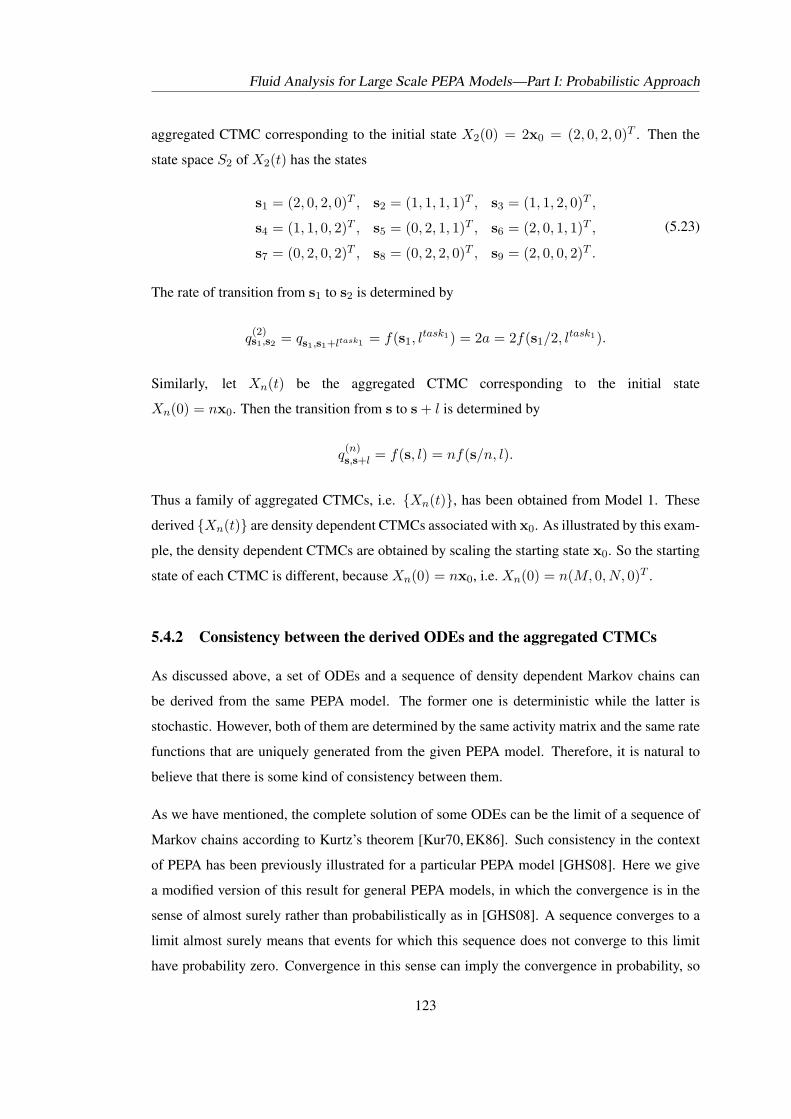
Fluid Analysis for Large Scale PEPA Models—Part I: Probabilistic Approach
aggregated CTMC corresponding to the initial state X2(0) = 2x0 = (2, 0, 2, 0)T . Then the
state space S2 of X2(t) has the states
s1 = (2, 0, 2, 0)T , s2 = (1, 1, 1, 1)T , s3 = (1, 1, 2, 0)T ,
s4 = (1, 1, 0, 2)T , s5 = (0, 2, 1, 1)T , s6 = (2, 0, 1, 1)T ,
s7 = (0, 2, 0, 2)T , s8 = (0, 2, 2, 0)T , s9 = (2, 0, 0, 2)T .
(5.23)
The rate of transition from s1 to s2 is determined by
q(2)s1,s2 = qs1,s1+ltask1 = f(s1, l
task1) = 2a = 2f(s1/2, ltask1).
Similarly, let Xn(t) be the aggregated CTMC corresponding to the initial state
Xn(0) = nx0. Then the transition from s to s + l is determined by
q(n)s,s+l = f(s, l) = nf(s/n, l).
Thus a family of aggregated CTMCs, i.e. {Xn(t)}, has been obtained from Model 1. These
derived {Xn(t)} are density dependent CTMCs associated with x0. As illustrated by this exam-
ple, the density dependent CTMCs are obtained by scaling the starting state x0. So the starting
state of each CTMC is different, because Xn(0) = nx0, i.e. Xn(0) = n(M, 0, N, 0)T .
5.4.2 Consistency between the derived ODEs and the aggregated CTMCs
As discussed above, a set of ODEs and a sequence of density dependent Markov chains can
be derived from the same PEPA model. The former one is deterministic while the latter is
stochastic. However, both of them are determined by the same activity matrix and the same rate
functions that are uniquely generated from the given PEPA model. Therefore, it is natural to
believe that there is some kind of consistency between them.
As we have mentioned, the complete solution of some ODEs can be the limit of a sequence of
Markov chains according to Kurtz’s theorem [Kur70, EK86]. Such consistency in the context
of PEPA has been previously illustrated for a particular PEPA model [GHS08]. Here we give
a modified version of this result for general PEPA models, in which the convergence is in the
sense of almost surely rather than probabilistically as in [GHS08]. A sequence converges to a
limit almost surely means that events for which this sequence does not converge to this limit
have probability zero. Convergence in this sense can imply the convergence in probability, so
123
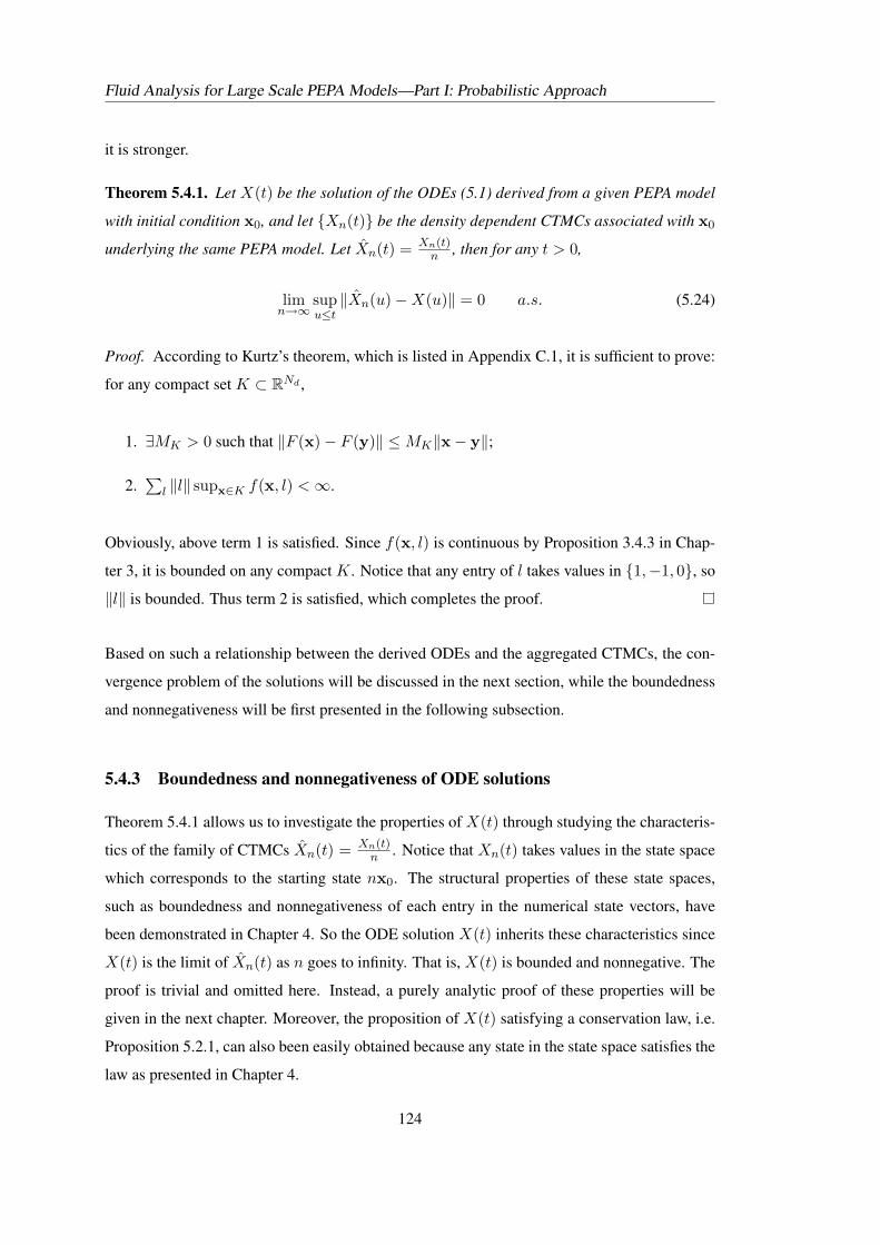
Fluid Analysis for Large Scale PEPA Models—Part I: Probabilistic Approach
it is stronger.
Theorem 5.4.1. Let X(t) be the solution of the ODEs (5.1) derived from a given PEPA model
with initial condition x0, and let {Xn(t)} be the density dependent CTMCs associated with x0
underlying the same PEPA model. Let Xn(t) = Xn(t)n , then for any t > 0,
limn→∞
supu≤t
‖Xn(u)−X(u)‖ = 0 a.s. (5.24)
Proof. According to Kurtz’s theorem, which is listed in Appendix C.1, it is sufficient to prove:
for any compact set K ⊂ RNd ,
1. ∃MK > 0 such that ‖F (x)− F (y)‖ ≤ MK‖x− y‖;
2.∑
l ‖l‖ supx∈K f(x, l) < ∞.
Obviously, above term 1 is satisfied. Since f(x, l) is continuous by Proposition 3.4.3 in Chap-
ter 3, it is bounded on any compact K. Notice that any entry of l takes values in {1,−1, 0}, so
‖l‖ is bounded. Thus term 2 is satisfied, which completes the proof.
Based on such a relationship between the derived ODEs and the aggregated CTMCs, the con-
vergence problem of the solutions will be discussed in the next section, while the boundedness
and nonnegativeness will be first presented in the following subsection.
5.4.3 Boundedness and nonnegativeness of ODE solutions
Theorem 5.4.1 allows us to investigate the properties of X(t) through studying the characteris-
tics of the family of CTMCs Xn(t) = Xn(t)n . Notice that Xn(t) takes values in the state space
which corresponds to the starting state nx0. The structural properties of these state spaces,
such as boundedness and nonnegativeness of each entry in the numerical state vectors, have
been demonstrated in Chapter 4. So the ODE solution X(t) inherits these characteristics since
X(t) is the limit of Xn(t) as n goes to infinity. That is, X(t) is bounded and nonnegative. The
proof is trivial and omitted here. Instead, a purely analytic proof of these properties will be
given in the next chapter. Moreover, the proposition of X(t) satisfying a conservation law, i.e.
Proposition 5.2.1, can also been easily obtained because any state in the state space satisfies the
law as presented in Chapter 4.
124
Fluid Analysis for Large Scale PEPA Models—Part I: Probabilistic Approach
Theorem 5.4.1 just states the approximation but does not state how to approximate the ODEs by
the family of CTMCs, i.e. it does not provide the error bounds of the approximation. Detailed
techniques and discussions of this topic have been presented in [DN08]. The reader is referred
to that paper since this thesis does not discuss this topic theoretically. However, experimental
results will be provided to show the error bounds of this kind of approximation (see the case
study in Chapter 7). Moreover, some other topics about the fluid approximations, such as the
comparison between accuracy and computational cost, numerical solution methods, and how to
derive performance measures from ODEs, will be discussed in detail in Chapter 7.
5.5 Convergence of ODE Solution: under a Particular Condition
Analogous to the steady-state probability distributions of the Markov chains underlying PEPA
models, upon which performance measures such as throughput and utilisation can be derived,
we expect the solution of the generated ODEs to have similar equilibrium conditions. In par-
ticular, if the solution has a limit as time goes to infinity we will be able to similarly obtain the
performance from the steady state, i.e. the limit. Therefore, whether the solution of the derived
ODEs converges becomes an important problem.
We should point out that Kurtz’s theorem cannot directly apply to the problem of whether or
not the solution the derived ODEs converges. This is because Kurtz’s theorem only deals with
the approximation between the ODEs and Markov chains during any finite time, rather than
considering the asymptotic behaviour of the ODEs as time goes to infinity. This section will
present our investigation and results about this problem.
We follow the assumptions in Theorem 5.4.1. Denote the expectation of Xn(t) as Mn(t), i.e.
Mn(t) = E[Xn(t)]. For any t, the stochastic processes {Xn(t)}n converge to the deterministic
X(t) when n tends to infinity, as Theorem 5.4.1 shows. It is not surprising to see that {Mn(t)}n,
the expectations of {Xn(t)}n, also converge to X(t) as n →∞:
Lemma 5.5.1. For any t,
limn→∞
Mn(t) = X(t).
Proof. Since X(t) is deterministic, then E[X(t)] = X(t). By Theorem 5.4.1, for all t, Xn(t)
converges to X(t) almost surely as n goes to infinity. Notice that Xn(t) is bounded (see the
discussion in Section 5.4.3), then by Lebesgue’s dominant convergence theorem given in Ap-
125
Fluid Analysis for Large Scale PEPA Models—Part I: Probabilistic Approach
pendix C.1, we have
limn→∞
E‖Xn(t)−X(t)‖ = 0.
Since a norm ‖ · ‖ can be considered as a convex function, by Jensen’s inequality (Theo-
rem2.2 [BZ99]), we have ‖(E[·])‖ ≤ E[‖ · ‖]. Therefore,
limn→∞
‖Mn(t)−X(t)‖ = limn→∞
‖E[Xn(t)]− E[X(t)]‖
≤ limn→∞
E‖Xn(t)−X(t)‖
= 0.
Lemma 5.5.1 states that the ODE solution X(t) is just the limit function of the sequence of
the expectation functions of the corresponding density dependent Markov chains. This pro-
vides some clues: the characteristics of the limit X(t) depend on the properties of {Mn(t)}n.
Therefore, we expect to be able to investigate X(t) by studying {Mn(t)}n.
Since Mn(t) is the expectation of the Markov chain Xn(t), Mn(t) can be expressed by a for-
mula in which the transient probability distribution is involved. That is,
Mn(t) = E[Xn(t)] =∑x∈Sn
xπnt (x),
where Sn is the state space, πnt (·) is the probability distribution of Xn at time t. Let Sn and
πnt (·) be the state space and the probability distribution of Xn(t) respectively2. Then
Mn(t) = E[Xn(t)] = E
[Xn(t)
n
]=∑x∈Sn
xn
πnt (x).
We have assumed the Markov chains underlying PEPA models to be irreducible and positive-
recurrent. Then the transient probability distributions of these Markov chains will converge to
the corresponding steady-state probability distributions. We denote the steady-state probability
distributions of Xn(t) and Xn(t) as πn∞(·) and πn
∞(·) respectively. Then, we have a lemma.
Lemma 5.5.2. For any n, there exists a Mn(∞), such that
limt→∞
Mn(t) = Mn(∞).
2We should point out that the probability distributions of Xn(t) and Xn(t) are the same, i.e. πnt (x) = πn
t (x/n).
126
Fluid Analysis for Large Scale PEPA Models—Part I: Probabilistic Approach
Proof.
limt→∞
Mn(t) = limt→∞
∑x∈Sn
xn
πnt (x)
=∑x∈Sn
limt→∞
xn
πnt (x)
=∑x∈Sn
xn
πn∞(x)
≡ Mn(∞).
Clearly, we also have Mn(∞) =∑
x∈Snxπn
∞(x).
Remark 5.5.1. Currently, we do not know whether the sequence {Mn(∞)}n converges as
n → ∞. But since {Mn(∞)}n is bounded which is due to the conservation law that PEPA
models satisfy, there exists {n′} ⊂ {n} such that {Mn′(∞)} converges to a limit, namely
M∞(∞). That is
limn′→∞
Mn′(∞) = M∞(∞).
Thus,
limn′→∞
limt→∞
Mn′(t) = limn′→∞
Mn′(∞) = M∞(∞). (5.25)
At the moment, there are two questions:
1. Whether limt→∞ limn′→∞ Mn′(t) exists?
2. If limt→∞ limn′→∞ Mn′(t) exists, whether
limt→∞
limn′→∞
Mn′(t) = limn′→∞
limt→∞
Mn′(t)?
If the answer to the first question is yes, then the solution of the ODEs converges, since by
Lemma 5.5.2,
limt→∞
X(t) = limt→∞
limn′→∞
Mn′(t).
If the answer to the second question is yes, then the limit of X(t) is consistent with the station-
127
Fluid Analysis for Large Scale PEPA Models—Part I: Probabilistic Approach
ary distributions of the Markov chains since
limt→∞
X(t) = limt→∞
limn′→∞
Mn′(t) = limn′→∞
limt→∞
Mn′(t) = M∞(∞).
Mn′(t)n′→∞−−−−−−−−−→
Lemma 5.5.1X(t)(= M∞(t))
t→∞yLemma 5.5.2 ???
yt→∞
Mn′(∞)Remark 5.5.1−−−−−−−−−→
n′→∞M∞(∞)
Figure 5.3: Convergence and consistency diagram for derived ODEs
In short, the positive answers to these two questions determine the convergence and consistency
for the ODE solution, see Figure 5.3. Fortunately, the two answers can be guaranteed by the
condition (5.26) in the following Proposition 5.5.1.
Proposition 5.5.1. (A particular condition) If there exist A,B > 0, such that
supn′
∥∥∥Mn′(t)− Mn′(∞)∥∥∥ < Be−At, (5.26)
then limt→∞X(t) = M∞(∞).
Proof.
∥∥∥X(t)− M∞(∞)∥∥∥ =
∥∥∥∥ limn′→∞
[Mn′(t)− Mn′(∞)]∥∥∥∥
≤ lim supn′→∞
∥∥∥Mn′(t)− Mn′(∞)∥∥∥
≤ lim supn′→∞
[supn′
∥∥∥Mn′(t)− Mn′(∞)∥∥∥]
≤ lim supn′→∞
Be−At
= Be−At −→ 0, as t −→∞.
So limt→∞X(t) = M∞(∞).
Notice that Mn(t) =∑x∈Sn
xn
πnt (x) and Mn(∞) =
∑x∈Sn
xn
πn∞(x), so in order to estimate∥∥∥Mn(t)− Mn(∞)
∥∥∥ in (5.26), we need first to estimate the difference between πnt and πn
∞.
128
Fluid Analysis for Large Scale PEPA Models—Part I: Probabilistic Approach
Lemma 5.5.3. If there exists A > 0 and B1 > 0, such that for any n′ and all x ∈ Sn′ ,
|πn′t (x)− πn′
∞(x)| ≤ πn′∞(x)B1e
−At, (5.27)
then there exists B > 0 such that supn′
∥∥∥Mn′(t)− Mn′(∞)∥∥∥ < Be−At holds.
Proof. We know that Xn(0) =Xn(0)
n= x0 for any n. By the conservation law, the population
of each entity in any state is determined by the starting state. So for any n′ and all x ∈ Sn′ ,
||x/n′|| ≤ C1∑
P∈D x0[P ] < ∞, whereD is the set of all local derivatives and C1 is a constant
independent of n′. Let C = supn′ maxx∈Sn′ ||x/n′||, then C < ∞.
∥∥∥Mn′(t)− Mn′(∞)∥∥∥ =
∥∥∥∥∥∥∑
x∈Sn′
xn′
πn′t (x)−
∑x∈Sn′
xn′
πn′∞(x)
∥∥∥∥∥∥=
∥∥∥∥∥∥∑
x∈Sn′
xn′
(πn′t (x)− πn′
∞(x))
∥∥∥∥∥∥≤ sup
n′maxx∈Sn′
∥∥∥ xn′
∥∥∥ ∑x∈Sn′
|πn′t (x)− πn′
∞(x)|
= C∑
x∈Sn′
|πn′t (x)− πn′
∞(x)|
≤ C∑
x∈Sn′
πn′∞(x)B1e
−tA
= CB1e−tA.
Let B = CB1. Then supn′
∥∥∥Mn′(t)− Mn′(∞)∥∥∥ < Be−At.
5.6 Investigation of the Particular Condition
This section will present the study of the particular condition (5.26). We will expose that the
condition is related to well-known constants of Markov chains such as the spectral gap and the
Log-Sobolev constant. The methods and results developed in the field of functional analysis of
Markov chains are utilised to investigate the condition.
129
Fluid Analysis for Large Scale PEPA Models—Part I: Probabilistic Approach
5.6.1 An important estimation in the context of Markov kernel
We first give an estimation for the Markov kernel which is defined below. Let Q be the in-
finitesimal generator of a Markov chain X on a finite state S. Let
Kij =
Qij
m , i 6= j
1 + Qii
m , i = jwhere m = sup
i(−Qii).
K is a transition probability matrix, satisfying
K(x,y) ≥ 0,∑y
K(x,y) = 1.
K is called an Markov kernel (K is also called the uniformisation of the CTMC in some liter-
ature). A Markov chain on a finite state space S can be described through its kernel K. The
continuous time semigroup associated with K is defined by
Ht = exp(−t(I −K)).
Let π be the unique stationary measure of the Markov chain. Then Ht(x,y) → π(y) as t tends
to infinity. Following the convention in the literature we will also use (K, π) to represent a
Markov chain.
Notice
Q = m(K − I), K =Q
m+ I.
Clearly,
Pt = etQ = emt(K−I) = e−mt(I−K) = Hmt,
and thus Ht = P tm
, where Pt is called the semigroup associated with the infinitesimal generator
Q. An estimation of Ht is given below.
Lemma 5.6.1. (Corollary 2.2.6, [SC97]) Let (K, π) be a finite Markov chain, and
π(∗) = minx∈S
π(x). Then
supx,y
∣∣∣∣Ht(x,y)π(y)
− 1∣∣∣∣ ≤ e2−c for t =
1α
log log1
π(∗)+
c
λ, (5.28)
where λ > 0, α > 0 are the spectral gap and the Log-Sobolev constant respectively, which are
defined and interpreted in Appendix C.2.
130
Fluid Analysis for Large Scale PEPA Models—Part I: Probabilistic Approach
It can be implied from (5.28) that ∀x,y ∈ S,
|Ht(x,y)− π(y)| ≤ π(y)[e2+ λ
αlog log 1
π(∗)]e−λt. (5.29)
Since Ht = P tm
, so
∣∣∣P tm
(x,y)− π(y)∣∣∣ ≤ π(y)
[e2+ λ
αlog log 1
π(∗)]e−λt, (5.30)
and thus (replacing “t” by “mt” on the both sides of (5.30)),
|Pt(x,y)− π(y)| ≤ π(y)[e2+ λ
αlog log 1
π(∗)]e−mλt. (5.31)
The investigation and utilisation of the formulae (5.31) will be presented in the next subsection.
5.6.2 Investigation of the particular condition
For each n, let Qn be the infinitesimal generator of the density dependent Markov chain Xn(t)
underlying a given PEPA model and thus the transition probability matrix is Pnt = etQn
. For
each Xn(t), the initial state of the corresponding system is nx0, so the initial probability distri-
bution of Xn(t) is πn0 (nx0) = 1 and πn
0 (x) = 0, ∀x ∈ Sn,x 6= nx0. So ∀y ∈ Sn,
πnt (y) =
∑x∈Sn
πn0 (x)Pn
t (x,y) = πn0 (nx0)Pn
t (nx0,y) = Pnt (nx0,y). (5.32)
The formula (5.31) in the context of Xn(t) is
|Pnt (x,y)− πn
∞(y)| ≤ πn∞(y)
[e2+ λn
αnlog log 1
πn∞(∗)
]e−mnλnt, (5.33)
where λn, λn,mn, πn∞(∗) are the respective parameters associated with Xn(t).
Let x = nx0 in (5.33), and notice Pnt (nx0,y) = πn
t (y) by (5.32), then we have
|πnt (y)− πn
∞(y)| ≤ πn∞(y)
[e2+ λn
αnlog log 1
πn∞(∗)
]e−mnλnt, ∀y ∈ Sn. (5.34)
From the comparison of (5.34) and (5.27), we know that if there are some conditions imposed
on λnαn
log log 1πn∞(∗) and −mnλnt, then (5.27) can be induced from (5.34). See the following
131
Fluid Analysis for Large Scale PEPA Models—Part I: Probabilistic Approach
Lemma.
Lemma 5.6.2. If there exists T > 0, B2 > 0, A > 0 such that
supn
{−mnλnT +
λn
αnlog log
1πn∞(∗)
}≤ B2, (5.35)
and
infn{mnλn} ≥ A, (5.36)
then
|πnt (x)− πn
∞(x)| ≤ πn∞(x)B1e
−At, ∀x ∈ Sn, (5.37)
where B1 = eA1T+B2+2, and the “particular condition” (5.26) holds.
Proof. [e2+ λn
αnlog log 1
πn∞(∗)
]e−mnλnt =
[e−mnαnT+2+ λn
αnlog log 1
πn∞(∗)
]e−mnλn(t−T )
≤ eB2+2e−A(t−T )
= B1e−At.
Then by (5.34), (5.37) holds. Thus by Lemma 5.5.3, (5.26) holds.
Remark 5.6.1. When n tends to infinity, the discrete space is approximating a continuous
space and thus the probability of any single point is tending to 0, that is πn∞(∗) tends to 0. So
log log 1πn∞(∗) →∞ as n goes to infinity. Notice that by Lemma C.2.1 in Appendix C.2,
λn
αn≤ log(1/πn
∞(∗)).
Therefore, in order to have
−mnλnT +λn
αnlog log
1πn∞(∗)
≤ B2,
it is sufficient to let
Tmnλn ≥ O([log(1/πn∞(∗))]2). (5.38)
Moreover, (5.38) can imply both (5.35) and (5.36).
According to the above analysis, our problem is simplified to checking that whether (5.38) is
132
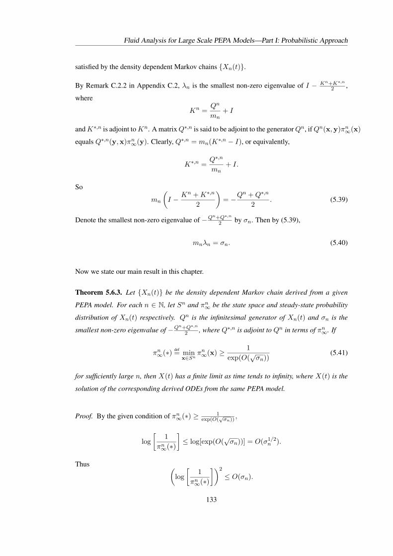
Fluid Analysis for Large Scale PEPA Models—Part I: Probabilistic Approach
satisfied by the density dependent Markov chains {Xn(t)}.
By Remark C.2.2 in Appendix C.2, λn is the smallest non-zero eigenvalue of I − Kn+K∗,n
2 ,
where
Kn =Qn
mn+ I
and K∗,n is adjoint to Kn. A matrix Q∗,n is said to be adjoint to the generator Qn, if Qn(x,y)πn∞(x)
equals Q∗,n(y,x)πn∞(y). Clearly, Q∗,n = mn(K∗,n − I), or equivalently,
K∗,n =Q∗,n
mn+ I.
So
mn
(I − Kn + K∗,n
2
)= −Qn + Q∗,n
2. (5.39)
Denote the smallest non-zero eigenvalue of −Qn+Q∗,n
2 by σn. Then by (5.39),
mnλn = σn. (5.40)
Now we state our main result in this chapter.
Theorem 5.6.3. Let {Xn(t)} be the density dependent Markov chain derived from a given
PEPA model. For each n ∈ N, let Sn and πn∞ be the state space and steady-state probability
distribution of Xn(t) respectively. Qn is the infinitesimal generator of Xn(t) and σn is the
smallest non-zero eigenvalue of −Qn+Q∗,n
2 , where Q∗,n is adjoint to Qn in terms of πn∞. If
πn∞(∗) def= min
x∈Snπn∞(x) ≥ 1
exp(O(√
σn))(5.41)
for sufficiently large n, then X(t) has a finite limit as time tends to infinity, where X(t) is the
solution of the corresponding derived ODEs from the same PEPA model.
Proof. By the given condition of πn∞(∗) ≥ 1
exp(O(√
σn)) ,
log[
1πn∞(∗)
]≤ log[exp(O(
√σn))] = O(σ1/2
n ).
Thus (log[
1πn∞(∗)
])2
≤ O(σn).
133
Fluid Analysis for Large Scale PEPA Models—Part I: Probabilistic Approach
Choose a large T such that
Tmnλn = Tσn ≥ O(σn) ≥(
log[
1πn∞(∗)
])2
.
By Remark 5.6.1 and Lemma 5.6.2, the particular condition holds. Therefore
limt→∞
X(t) = M∞(∞).
According to the above theorem, our problem is simplified to checking that whether (5.41) is
satisfied by the density dependent Markov chains {Xn(t)}. In (5.41) both the spectral gap
λn (= σnmn
) and πn∞(∗) are unknown. In fact, due to the state space explosion problem, πn
∞
cannot be easily solved from πn∞Qn = 0 or equivalently πn
∞Kn = πn∞. Moreover, the estima-
tion of the spectral gap in current literature, for a given Markov chain, is heavily based on the
known stationary distribution, see Theorem C.2.2 and Theorem C.2.3 in Appendix C.2. Thus,
these current results cannot provide a practical check for (5.41).
The convergence and consistency are supported by many numerical experiments (see the case
study in Chapter 7), so we believe that (5.41) is unnecessary. In other words, we believe (5.41)
always holds in the context of PEPA, although at this moment we cannot prove it. Before
concluding this section, we leave an open problem:
Conjecture 1. The formula (5.41) in Theorem 5.6.3 holds for any PEPA model.
5.7 Summary
This chapter has presented the semantics of mapping general PEPA models to ODEs, which
generalises the results of fluid approximations for PEPA in current literature. The fundamental
characteristics of the solutions of the derived ODEs, such as existence, uniqueness, nonneg-
ativeness, boundedness, convergence, as well as the consistency with the underlying Markov
chains, have been established in this chapter. For convenience, we organise them into the fol-
lowing Table 5.5.
In particular, for nonsynchronised PEPA models, as time goes to infinity the solutions of the
derived ODEs have finite limits, which coincide with the stationary probability distributions
134
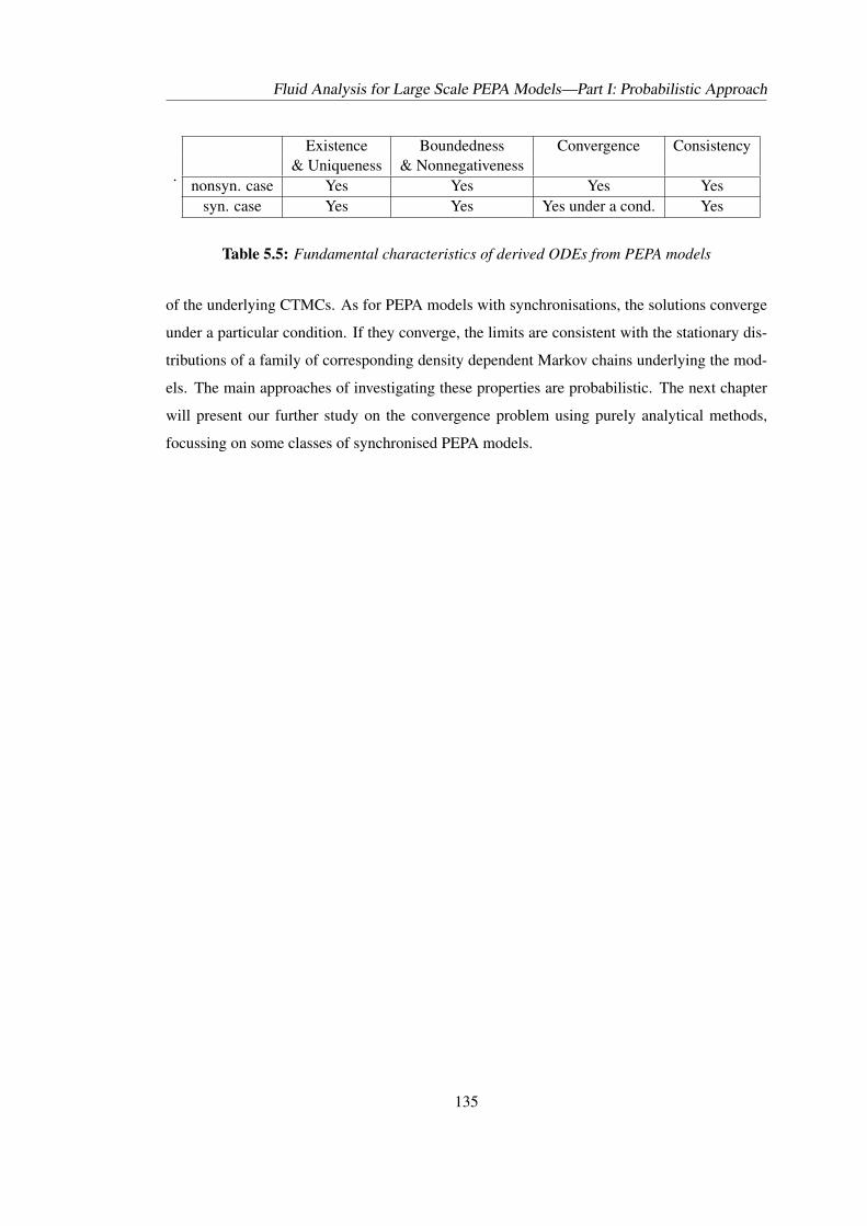
Fluid Analysis for Large Scale PEPA Models—Part I: Probabilistic Approach
.
Existence Boundedness Convergence Consistency& Uniqueness & Nonnegativeness
nonsyn. case Yes Yes Yes Yessyn. case Yes Yes Yes under a cond. Yes
Table 5.5: Fundamental characteristics of derived ODEs from PEPA models
of the underlying CTMCs. As for PEPA models with synchronisations, the solutions converge
under a particular condition. If they converge, the limits are consistent with the stationary dis-
tributions of a family of corresponding density dependent Markov chains underlying the mod-
els. The main approaches of investigating these properties are probabilistic. The next chapter
will present our further study on the convergence problem using purely analytical methods,
focussing on some classes of synchronised PEPA models.
135

136
Chapter 6Fluid Analysis for Large Scale PEPA
Models—Part II: Analytical Approach
6.1 Introduction
The previous chapter has demonstrated the fluid approximation and relevant analysis for PEPA.
Some fundamental results about the derived ODEs such as the boundedness, nonnegativeness
and convergence of the solutions, have been established through a probabilistic approach. In
this chapter we will discuss the boundedness and nonnegativeness again, and prove them by
a purely analytical argument. The convergence presented in the previous chapter is proved
under a particular condition that cannot currently be easily checked. This chapter will present
alternative approaches to deal with the convergence problem. In particular, for an interesting
model with two synchronisations, its structural invariance as revealed in Chapter 4, will be
shown to play an important role in the proof of the convergence. Moreover, for a class of
PEPA models which have two component types and one synchronisation, an analytical proof
of the convergence under some mild conditions on the populations will be presented. These
discussions and investigations will provide new insight into the fluid approximation of PEPA.
The remainder of this chapter is structured as follows. Section 2 gives a purely analytical proof
for the boundedness and nonnegativeness of the solutions of the ODEs derived from general
PEPA models. A case study on convergence for a model with two synchronisations will be
shown in Section 3. In Sections 4 and 5, we present proofs of convergence for PEPA models
with two component types and one synchronisation. Finally, Section 6 concludes this chapter.
6.2 Analytical Proof of Boundedness and Nonnegativeness
Recall that the set of derived ODEs from a general PEPA model is
dxdt
=∑
l∈Alabel
lf(x, l). (6.1)
137
Fluid Analysis for Large Scale PEPA Models—Part II: Analytical Approach
In the previous chapter we have proved that the solution of (6.1) is bounded as well as nonneg-
ative. This section will present a new analytical proof for these characteristics.
6.2.1 Features of the derived ODEs
Let U be a local derivative, then from (6.1) we have
dx(U, t)dt
= −∑
{l|U∈pre(l)}
f(x, l) +∑
{l|U∈post(l)}
f(x, l). (6.2)
As mentioned in Chapter 5, in this formula the term∑
{l|U∈pre(l)} f(x, l) represents the exit
rates in the local derivative U , while the term∑
{l|U∈post(l)} f(x, l) indicates the entry rates to
U . We have noted an important fact: all exit rates in a component type are balanced by all entry
rates. That is Proposition 5.2.1 in Chapter 5. Below, for convenience, this proposition is stated
again:
Proposition 5.2.1. Let Cij be the local derivatives of component type Ci. Then for any i and
t,∑
j
dx(Cij , t
)dt
= 0, and∑
j x(Cij , t
)=∑
j x(Cij , 0
).
This proposition states that the ODEs (6.1) satisfy a conservation law: at any time the popula-
tion of each component type is constant, since the system is closed and there is no exchange
with the environment.
Another important fact to note is: the exit rates in a local derivative Cij in state x are bounded
by all the apparent rates in this local derivative. In fact, according to Proposition 3.4.2 in
Chapter 3, if Cij ∈ pre(l) where l is a labelled activity, then the transition rate function f(x, l)
is bounded by rl(x, Cij ), the apparent rates of l in Cij in state x. That is, f(x, l) ≤ rl(x, Cij ).
Notice rl(x, Cij ) = x[Cij ]rl(Cij ) by Definition 3.4.1 in Chapter 3, where rl(Cij ) represents
the apparent rate for a single instance of Cij . Thus, we have
f(x, l) ≤ x[Cij ]rl(Cij ). (6.3)
We should point out that (6.3) is based on the discrete state space underlying the given model.
According to our semantics of mapping PEPA model to ODEs, the fluid approximation-version
of (6.3) also holds, i.e. f(x(t), l) ≤ x(Cij , t)rl(Cij ). Therefore, we have the following
138
Fluid Analysis for Large Scale PEPA Models—Part II: Analytical Approach
Proposition 6.2.1. For any local derivative Cij ,
∑{l|Cij
∈pre(l)}
f(x(t), l) ≤ x(Cij , t)∑
{l|Cij∈pre(l)}
rl(Cij ), (6.4)
where rl(Cij ) is the apparent rate of l in Cij for a single instance of Cij defined in Defini-
tion 3.4.1.
Propositions 5.2.1 and 6.2.1 are two important characteristics of the ODEs derived from PEPA
models, which can guarantee the boundedness and nonnegativeness of the solutions.
6.2.2 Boundedness and nonnegativeness of solutions
We know that the solution of (6.1) exists and is unique. Furthermore, the solution is bounded
and nonnegative, which has been proved in the previous chapter through an approximation
approach. This subsection will present an analytical proof of these properties, based on the two
propositions described in the previous subsection.
Suppose the initial values x(Cij , 0
)are given, and we denote
∑j x(Cij , 0
)by NCi . We have
a theorem:
Theorem 6.2.1. If x(Cij , t
)satisfies (6.1) with nonnegative initial values, then
0 ≤ x(Cij , t
)≤ NCi , for any t ≥ 0. (6.5)
Moreover, if the initial values are positive, then the solutions are always positive, i.e.,
0 < x(Cij , t
)< NCi , for any t ≥ 0. (6.6)
Proof. By Proposition 5.2.1,∑
j x(Cij , t
)= NCi for all t. All that is left to do is to prove that
x(Cij , t) is positive or nonnegative. The proof is divided into two cases.
Case 1: Suppose all the initial values are positive, i.e. minij
{x(Cij , 0)
}> 0. We will
show that minij
{x(Cij , t)
}> 0 for all t ≥ 0. Otherwise, if there exists a t > 0 such that
minij
{x(Cij , t)
}≤ 0, then there exists a point t′ > 0 such that minij
{x(Cij , t
′)}
= 0. Let
139
Fluid Analysis for Large Scale PEPA Models—Part II: Analytical Approach
t∗ be the first such point, i.e.
t∗ = inf{
t > 0 | minij
{x(Cij , t)
}= 0}
,
then 0 < t∗ < ∞. Without loss of generality, we assume x(C11 , t) reaches zero at t∗, i.e.,
x(C11 , t∗) = 0, x(Cij , t
∗) ≥ 0 (i 6= 1 ∨ j 6= 1)
and
x(Cij , t) > 0, t ∈ [0, t∗), ∀i, j.
Notice that the transition rate function is nonnegative (see Proposition 3.4.2), i.e. f(x, l) ≥ 0.
Then for t ∈ [0, t∗], by Proposition 6.2.1,
dx(C11 , t)dt
= −∑
{l|C11∈pre(l)}
f(x, l) +∑
{l|C11∈post(l)}
f(x, l)
≥ −∑
{l|C11∈pre(l)}
f(x, l)
≥ −x(C11 , t)∑
{l|C11∈pre(l)}
rl(C11).
Set R =∑
{l|C11∈pre(l)} rl(C11), then
dx(C11 , t)dt
≥ −Rx(C11 , t). (6.7)
By Lemma D.1.1 in Appendix D.1, (6.7) implies
x(C11 , t∗) ≥ x(C11 , 0)e−Rt∗ > 0.
This is a contradiction to x(C11 , t∗) = 0. Therefore 0 < x
(Cij , t
), and thus by Proposi-
tion 5.2.1,
0 < x(Cij , t
)< NC0 , ∀t.
Case 2: Suppose minij
{x(Cij , 0)
}= 0. Let uδ(ij , 0) = x(Cij , 0) + δ where δ > 0. Let
uδ(ij , t) be the solution of (6.1), given the initial value uδ(ij , 0). By the proof of Case 1,
uδ(ij , t) > 0 (∀t ≥ 0). Noticing min(·) is a Lipschitz function, by the Fundamental Inequality
140
Fluid Analysis for Large Scale PEPA Models—Part II: Analytical Approach
(Theorem D.1.2) in Appendix D.1, we have
|uδ(ij , t)− x(Cij , t)| ≤ δeKt, (6.8)
where K is a constant. Thus, for any given t ≥ 0,
x(Cij , t) ≥ uδ(ij , t)− δeKt > −δeKt. (6.9)
Let δ ↓ 0 in (6.9), then we have x(Cij , t) ≥ 0. The proof is completed.
6.3 A Case Study on Convergence with Two Synchronisations
If a model has synchronisations, then the derived ODEs are nonlinear. The nonlinearity results
in the complexity of the dynamic behaviour of fluid approximations. However, for some special
models, we can still determine the convergence of the solutions. What follows is a case study
for an interesting PEPA model, in which the structural property of invariance will be shown to
play an important role in the proof of the convergence.
6.3.1 ODEs derived from an interesting model
The model considered in this section is given below, which is Model 3 presented in Chapter 4.
X1def= (action1 , a1 ).X2
X2def= (action2 , a2 ).X1
Y1def= (action1 , a1 ).Y3 + (job1 , c1 ).Y2
Y2def= (job2 , c2 ).Y1
Y3def= (job3 , c3 ).Y4
Y4def= (action2 , a2 ).Y2 + (job4 , c4 ).Y3
(X1 [M1 ]||X2 [M2 ]) BC{action1,action2}
(Y1 [N1 ]||Y2 [N2 ]||Y3 [N3 ]||Y4 [N4 ]) .
The operations of X and Y are illustrated in Figure 6.1. According to the mapping semantics,
the derived ODEs from this model are
141
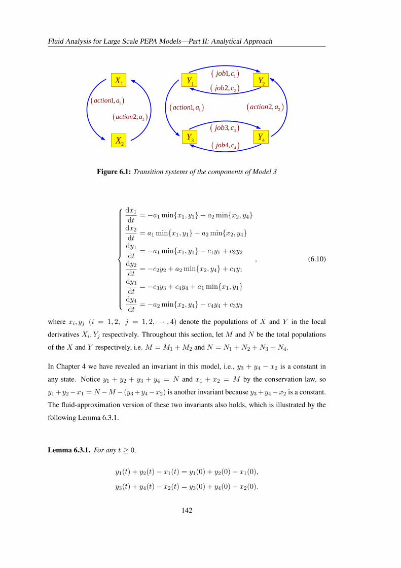
Fluid Analysis for Large Scale PEPA Models—Part II: Analytical Approach
( )11,action a
( )22,action a( )11,action a ( )22,action a
( )11,job c
( )22,job c
( )33,job c
( )44,job c
1X
2X
1Y 2Y
3Y 4Y
Figure 6.1: Transition systems of the components of Model 3
dx1
dt= −a1 min{x1, y1}+ a2 min{x2, y4}
dx2
dt= a1 min{x1, y1} − a2 min{x2, y4}
dy1
dt= −a1 min{x1, y1} − c1y1 + c2y2
dy2
dt= −c2y2 + a2 min{x2, y4}+ c1y1
dy3
dt= −c3y3 + c4y4 + a1 min{x1, y1}
dy4
dt= −a2 min{x2, y4} − c4y4 + c3y3
, (6.10)
where xi, yj (i = 1, 2, j = 1, 2, · · · , 4) denote the populations of X and Y in the local
derivatives Xi, Yj respectively. Throughout this section, let M and N be the total populations
of the X and Y respectively, i.e. M = M1 + M2 and N = N1 + N2 + N3 + N4.
In Chapter 4 we have revealed an invariant in this model, i.e., y3 + y4 − x2 is a constant in
any state. Notice y1 + y2 + y3 + y4 = N and x1 + x2 = M by the conservation law, so
y1 +y2−x1 = N −M − (y3 +y4−x2) is another invariant because y3 +y4−x2 is a constant.
The fluid-approximation version of these two invariants also holds, which is illustrated by the
following Lemma 6.3.1.
Lemma 6.3.1. For any t ≥ 0,
y1(t) + y2(t)− x1(t) = y1(0) + y2(0)− x1(0),
y3(t) + y4(t)− x2(t) = y3(0) + y4(0)− x2(0).
142
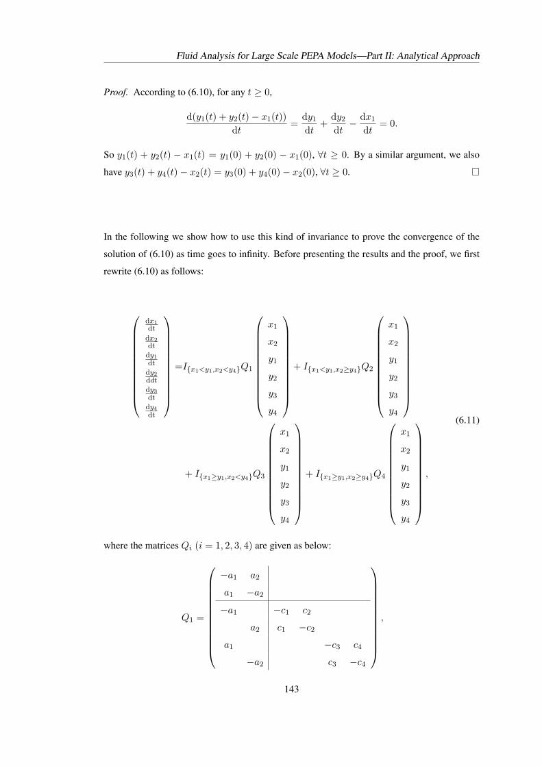
Fluid Analysis for Large Scale PEPA Models—Part II: Analytical Approach
Proof. According to (6.10), for any t ≥ 0,
d(y1(t) + y2(t)− x1(t))dt
=dy1
dt+
dy2
dt− dx1
dt= 0.
So y1(t) + y2(t) − x1(t) = y1(0) + y2(0) − x1(0), ∀t ≥ 0. By a similar argument, we also
have y3(t) + y4(t)− x2(t) = y3(0) + y4(0)− x2(0), ∀t ≥ 0.
In the following we show how to use this kind of invariance to prove the convergence of the
solution of (6.10) as time goes to infinity. Before presenting the results and the proof, we first
rewrite (6.10) as follows:
dx1dt
dx2dt
dy1
dt
dy2
ddt
dy3
dt
dy4
dt
=I{x1<y1,x2<y4}Q1
x1
x2
y1
y2
y3
y4
+ I{x1<y1,x2≥y4}Q2
x1
x2
y1
y2
y3
y4
+ I{x1≥y1,x2<y4}Q3
x1
x2
y1
y2
y3
y4
+ I{x1≥y1,x2≥y4}Q4
x1
x2
y1
y2
y3
y4
,
(6.11)
where the matrices Qi (i = 1, 2, 3, 4) are given as below:
Q1 =
−a1 a2
a1 −a2
−a1 −c1 c2
a2 c1 −c2
a1 −c3 c4
−a2 c3 −c4
,
143
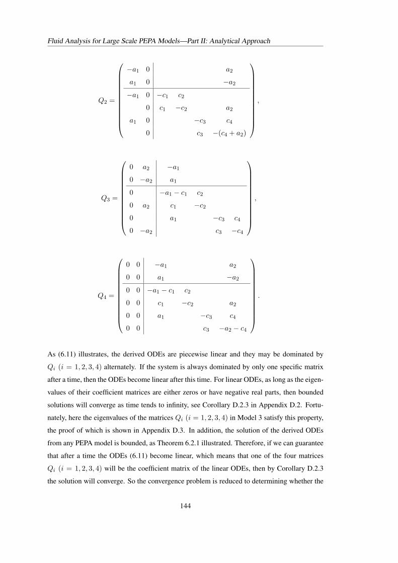
Fluid Analysis for Large Scale PEPA Models—Part II: Analytical Approach
Q2 =
−a1 0 a2
a1 0 −a2
−a1 0 −c1 c2
0 c1 −c2 a2
a1 0 −c3 c4
0 c3 −(c4 + a2)
,
Q3 =
0 a2 −a1
0 −a2 a1
0 −a1 − c1 c2
0 a2 c1 −c2
0 a1 −c3 c4
0 −a2 c3 −c4
,
Q4 =
0 0 −a1 a2
0 0 a1 −a2
0 0 −a1 − c1 c2
0 0 c1 −c2 a2
0 0 a1 −c3 c4
0 0 c3 −a2 − c4
.
As (6.11) illustrates, the derived ODEs are piecewise linear and they may be dominated by
Qi (i = 1, 2, 3, 4) alternately. If the system is always dominated by only one specific matrix
after a time, then the ODEs become linear after this time. For linear ODEs, as long as the eigen-
values of their coefficient matrices are either zeros or have negative real parts, then bounded
solutions will converge as time tends to infinity, see Corollary D.2.3 in Appendix D.2. Fortu-
nately, here the eigenvalues of the matrices Qi (i = 1, 2, 3, 4) in Model 3 satisfy this property,
the proof of which is shown in Appendix D.3. In addition, the solution of the derived ODEs
from any PEPA model is bounded, as Theorem 6.2.1 illustrated. Therefore, if we can guarantee
that after a time the ODEs (6.11) become linear, which means that one of the four matrices
Qi (i = 1, 2, 3, 4) will be the coefficient matrix of the linear ODEs, then by Corollary D.2.3
the solution will converge. So the convergence problem is reduced to determining whether the
144
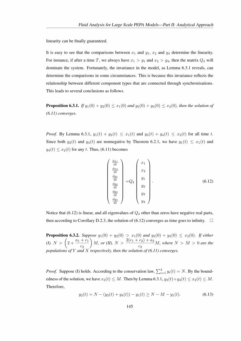
Fluid Analysis for Large Scale PEPA Models—Part II: Analytical Approach
linearity can be finally guaranteed.
It is easy to see that the comparisons between x1 and y1, x2 and y4 determine the linearity.
For instance, if after a time T , we always have x1 > y1 and x2 > y4, then the matrix Q4 will
dominate the system. Fortunately, the invariance in the model, as Lemma 6.3.1 reveals, can
determine the comparisons in some circumstances. This is because this invariance reflects the
relationship between different component types that are connected through synchronisations.
This leads to several conclusions as follows.
Proposition 6.3.1. If y1(0) + y2(0) ≤ x1(0) and y3(0) + y4(0) ≤ x2(0), then the solution of
(6.11) converges.
Proof. By Lemma 6.3.1, y1(t) + y2(t) ≤ x1(t) and y3(t) + y4(t) ≤ x2(t) for all time t.
Since both y2(t) and y4(t) are nonnegative by Theorem 6.2.1, we have y1(t) ≤ x1(t) and
y4(t) ≤ x2(t) for any t. Thus, (6.11) becomes
dx1dt
dx2dt
dy1
dt
dy2
dt
dy3
dt
dy4
dt
=Q4
x1
x2
y1
y2
y3
y4
. (6.12)
Notice that (6.12) is linear, and all eigenvalues of Q4 other than zeros have negative real parts,
then according to Corollary D.2.3, the solution of (6.12) converges as time goes to infinity.
Proposition 6.3.2. Suppose y1(0) + y2(0) > x1(0) and y3(0) + y4(0) ≤ x2(0). If either
(I). N >
(2 +
a1 + c1
c2
)M , or (II). N >
2(c1 + c2) + a2
c2M , where N > M > 0 are the
populations of Y and X respectively, then the solution of (6.11) converges.
Proof. Suppose (I) holds. According to the conservation law,∑4
i=1 yi(t) = N . By the bound-
edness of the solution, we have x2(t) ≤ M . Then by Lemma 6.3.1, y3(t)+y4(t) ≤ x2(t) ≤ M .
Therefore,
y2(t) = N − (y3(t) + y4(t))− y1(t) ≥ N −M − y1(t). (6.13)
145
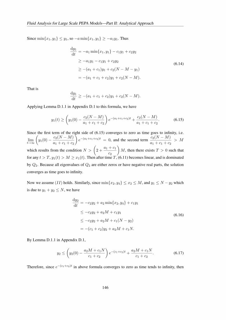
Fluid Analysis for Large Scale PEPA Models—Part II: Analytical Approach
Since min{x1, y1} ≤ y1, so −amin{x1, y1} ≥ −a1y1. Thus
dy1
dt= −a1 min{x1, y1} − c1y1 + c2y2
≥ −a1y1 − c1y1 + c2y2
≥ −(a1 + c1)y1 + c2(N −M − y1)
= −(a1 + c1 + c2)y1 + c2(N −M).
(6.14)
That isdy1
dt≥ −(a1 + c1 + c2)y1 + c2(N −M).
Applying Lemma D.1.1 in Appendix D.1 to this formula, we have
y1(t) ≥(
y1(0)− c2(N −M)a1 + c1 + c2
)e−(a1+c1+c2)t +
c2(N −M)a1 + c1 + c2
. (6.15)
Since the first term of the right side of (6.15) converges to zero as time goes to infinity, i.e.
limt→∞
(y1(0)− c2(N −M)
a1 + c1 + c2
)e−(a1+c1+c2)t = 0, and the second term
c2(N −M)a1 + c1 + c2
> M
which results from the condition N >
(2 +
a1 + c1
c2
)M , then there exists T > 0 such that
for any t > T , y1(t) > M ≥ x1(t). Then after time T , (6.11) becomes linear, and is dominated
by Q2. Because all eigenvalues of Q2 are either zeros or have negative real parts, the solution
converges as time goes to infinity.
Now we assume (II) holds. Similarly, since min{x2, y4} ≤ x2 ≤ M , and y1 ≤ N − y2 which
is due to y1 + y2 ≤ N , we have
dy2
dt= −c2y2 + a2 min{x2, y4}+ c1y1
≤ −c2y2 + a2M + c1y1
≤ −c2y2 + a2M + c1(N − y2)
= −(c1 + c2)y2 + a2M + c1N.
(6.16)
By Lemma D.1.1 in Appendix D.1,
y2 ≤(
y2(0)− a2M + c1N
c1 + c2
)e−(c1+c2)t +
a2M + c1N
c1 + c2. (6.17)
Therefore, since e−(c1+c2)t in above formula converges to zero as time tends to infinity, then
146
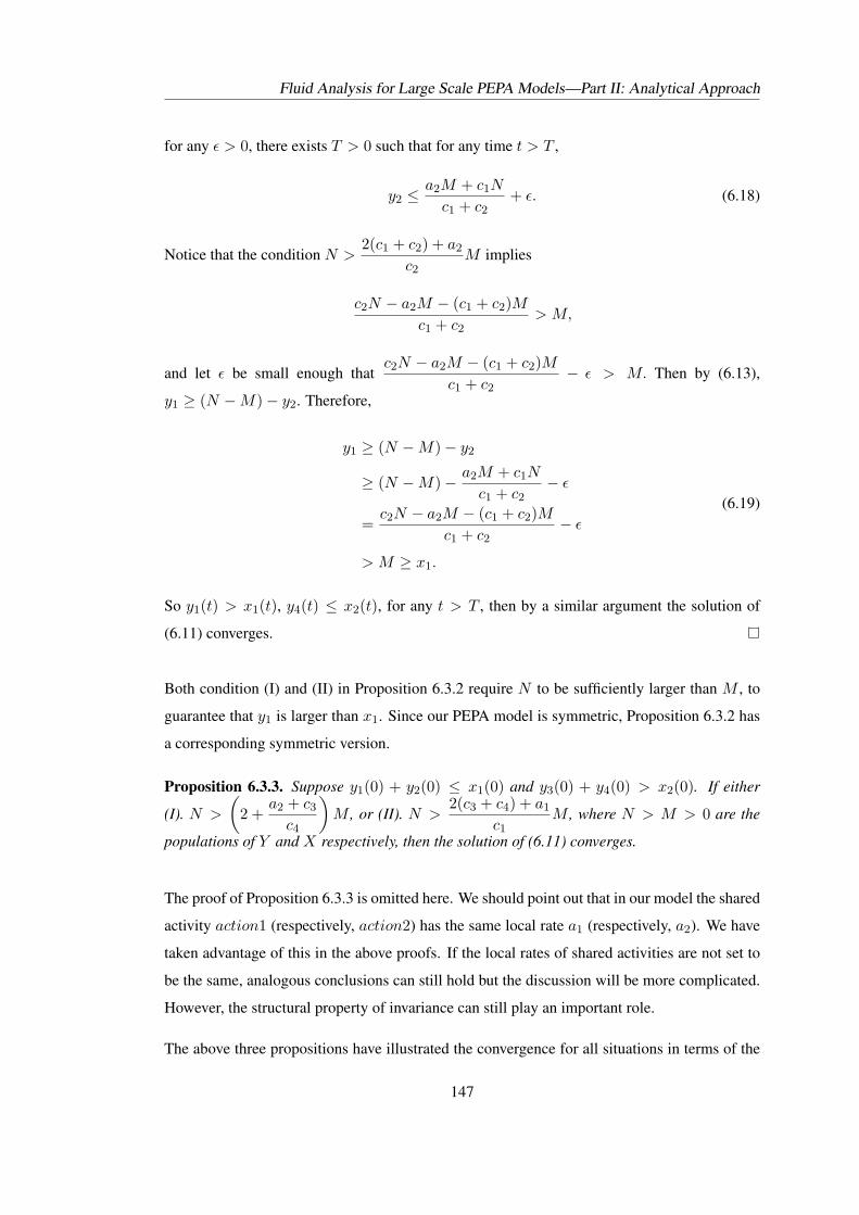
Fluid Analysis for Large Scale PEPA Models—Part II: Analytical Approach
for any ε > 0, there exists T > 0 such that for any time t > T ,
y2 ≤a2M + c1N
c1 + c2+ ε. (6.18)
Notice that the condition N >2(c1 + c2) + a2
c2M implies
c2N − a2M − (c1 + c2)Mc1 + c2
> M,
and let ε be small enough thatc2N − a2M − (c1 + c2)M
c1 + c2− ε > M. Then by (6.13),
y1 ≥ (N −M)− y2. Therefore,
y1 ≥ (N −M)− y2
≥ (N −M)− a2M + c1N
c1 + c2− ε
=c2N − a2M − (c1 + c2)M
c1 + c2− ε
> M ≥ x1.
(6.19)
So y1(t) > x1(t), y4(t) ≤ x2(t), for any t > T , then by a similar argument the solution of
(6.11) converges.
Both condition (I) and (II) in Proposition 6.3.2 require N to be sufficiently larger than M , to
guarantee that y1 is larger than x1. Since our PEPA model is symmetric, Proposition 6.3.2 has
a corresponding symmetric version.
Proposition 6.3.3. Suppose y1(0) + y2(0) ≤ x1(0) and y3(0) + y4(0) > x2(0). If either
(I). N >
(2 +
a2 + c3
c4
)M , or (II). N >
2(c3 + c4) + a1
c1M , where N > M > 0 are the
populations of Y and X respectively, then the solution of (6.11) converges.
The proof of Proposition 6.3.3 is omitted here. We should point out that in our model the shared
activity action1 (respectively, action2) has the same local rate a1 (respectively, a2). We have
taken advantage of this in the above proofs. If the local rates of shared activities are not set to
be the same, analogous conclusions can still hold but the discussion will be more complicated.
However, the structural property of invariance can still play an important role.
The above three propositions have illustrated the convergence for all situations in terms of the
147

Fluid Analysis for Large Scale PEPA Models—Part II: Analytical Approach
starting state, except for the case of y1(0) + y2(0) > x1(0), y3(0) + y4(0) > x2(0). See a
summary in Table 6.1. If y1(0) + y2(0) > x1(0), y3(0) + y4(0) > x2(0), then the dynamic
behaviour of the system is rather complex. A numerical study for this case will be presented in
the next subsection.
Starting state condition Additional condition Conclusiony1(0) + y2(0) ≤ x1(0), y3(0) + y4(0) ≤ x2(0) No Proposition 6.3.1y1(0) + y2(0) > x1(0), y3(0) + y4(0) ≤ x2(0) N > k1M Proposition 6.3.2y1(0) + y2(0) ≤ x1(0), y3(0) + y4(0) > x2(0) N > k2M Proposition 6.3.3
y1(0) + y2(0) > x1(0), y3(0) + y4(0) > x2(0) None identifiedExplorednumerically
Table 6.1: A summary for the convergence of Model 3
0 1 2 3 4 5 6 7 8 9 100
0.5
1
1.5
2
2.5
3
3.5
4
4.5
5
time
x1
x2
y1
y2
y3
y4
Figure 6.2: Numerical study for Model 3: rates (1, 1, 1, 1, 1, 1); equilibrium point(1, 1, 2, 3, 3, 2). (Note: the curves of x1 and x2, the curves of y1 and y4, as well asthose of y2 and y3 respectively, completely overlap.)
6.3.2 Numerical study for convergence
This subsection presents a numerical study at different action rate conditions. The starting
state in this subsection is always assumed as (1, 1, 5, 0, 0, 5), which satisfies the condition of
y1(0) + y2(0) > x1(0) and y3(0) + y4(0) > x2(0).
If all the action rates in the model are set to one, i.e. (a1, a2, c1, c2, c3, c4) = (1, 1, 1, 1, 1, 1),
then the equilibrium point of the ODEs is (x∗1, x∗2, y
∗1, y
∗2, y
∗3, y
∗4) = (1, 1, 2, 3, 3, 2), as the
148
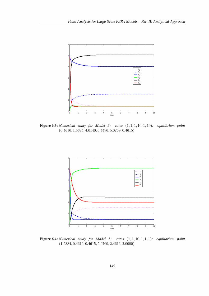
Fluid Analysis for Large Scale PEPA Models—Part II: Analytical Approach
0 1 2 3 4 5 6 7 8 9 100
1
2
3
4
5
6
time
x1
x2
y1
y2
y3
y4
Figure 6.3: Numerical study for Model 3: rates (1, 1, 1, 10, 1, 10); equilibrium point(0.4616, 1.5384, 4.0140, 0.4476, 5.0769, 0.4615)
0 1 2 3 4 5 6 7 8 9 100
1
2
3
4
5
6
time
x1
x2
y1
y2
y3
y4
Figure 6.4: Numerical study for Model 3: rates (1, 1, 10, 1, 1, 1); equilibrium point(1.5384, 0.4616, 0.4615, 5.0769, 2.4616, 2.0000)
149
Fluid Analysis for Large Scale PEPA Models—Part II: Analytical Approach
0 1 2 3 4 5 6 7 8 9 100
0.5
1
1.5
2
2.5
3
3.5
4
4.5
5
time
x1
x2
y1
y2
y3
y4
Figure 6.5: Numerical study for Model 3: rates (20, 20, 1, 1, 1, 1); equilibrium point(1, 1, 0.2273, 4.7727, 4.7727, 0.2273). (Note: the curves of x1 and x2, the curvesof y1 and y4, as well as those of y2 and y3 respectively, completely overlap.)
numerical solution of the ODEs illustrates. In this case, the matrix Q1 finally dominates the
system. See Figure 6.2. Notice that in this figure, the curves of x1 and x2 completely overlap,
as well as the curves of y1 and y4, and those of y2 and y3.
In other situations, for example, if (a1, a2, c1, c2, c3, c4) = (1, 1, 1, 10, 1, 10) then the equilib-
rium point is (0.4616, 1.5384, 4.0140, 0.4476, 5.0769, 0.4615), and the matrix Q2 eventually
dominates the system. See Figure 6.3. Moreover, the matrices Q3 and Q4 can also finally
dominate the system as long as the action rates are appropriately specified. See Figure 6.4 and
Figure 6.5. We should point out that similarly to Figure 6.2, in Figure 6.5 the curves of x1 and
x2, the curves of y1 and y4, as well as those of y2 and y3 respectively, completely overlap.
In short, the system dynamics is rather complex in the situation of y1(0) + y2(0) > x1(0) and
y3(0) + y4(0) > x2(0). A summary of these numerical studies is organised in Table 6.2.
Rates: Equilibrium points: Dominator Figure(a1, a2, c1, c2, c3, c4) (x∗1, x
∗2, y
∗1 , y∗2 , y∗3 , y∗4)
(1, 1, 1, 1, 1, 1) (1, 1, 2, 3, 3, 2) Q1 Figure 6.2(1, 1, 1, 10, 1, 10) (0.4616, 1.5384, 4.0140, 0.4476, 5.0769, 0.4615) Q2 Figure 6.3(1, 1, 10, 1, 1, 1) (1.5384, 0.4616, 0.4615, 5.0769, 2.4616, 2.0000) Q3 Figure 6.4(20, 20, 1, 1, 1, 1) (1, 1, 0.2273, 4.7727, 4.7727, 0.2273) Q4 Figure 6.5
Table 6.2: Complex dynamical behaviour of Model 3: starting state (1,1,5,0,0,5)
150
Fluid Analysis for Large Scale PEPA Models—Part II: Analytical Approach
6.4 Convergence For Two Component Types and One Synchroni-
sation (I): A Special Case
The problem of convergence for more general models without strict conditions, is rather com-
plex and has not been completely solved. But for a particular class of PEPA model — a model
composed of two types of component with one synchronisation between them, we can deter-
mine the convergence of the solutions of the derived ODEs.
As discussed in the previous section, the ODEs derived from PEPA are piecewise linear and
may be dominated by different coefficient matrices alternately. For any PEPA model which has
two component types and one synchronisation, the two corresponding coefficient matrices can
be proved to have a good property: their eigenvalues are either zeros or have negative real parts.
The remaining issue for convergence is to ascertain that these two matrices will not always
alternately dominate the system. In fact, we will prove that under some mild conditions, there
exists a time after which there is only one coefficient matrix dominating the system. This means
the ODEs become linear after that time. Since the coefficient matrix of the linear ODEs satisfies
the good eigenvalue property, then by Corollary D.2.3, the bounded solution will converge as
time goes to infinity.
We first utilise an example in this section to show our approach to dealing with the convergence
problem for this class of PEPA models. The proof for a general case in this class is presented
in the next section.
6.4.1 A previous model and the derived ODE
Let us look at the following PEPA model, which is Model 1 presented in Chapter 1:
User1def=(task1, a).User2
User2def=(task2, b).User1
Provider1def=(task1, a).P rovider2
Provider2def=(reset, d).P rovider1
(User1[M ]) BC{task1}
(Provider1[N ]).
151
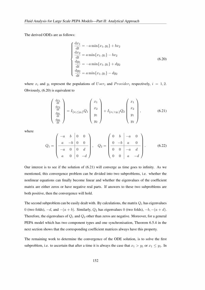
Fluid Analysis for Large Scale PEPA Models—Part II: Analytical Approach
The derived ODEs are as follows:
dx1
dt= −amin{x1, y1}+ bx2
dx2
dt= amin{x1, y1} − bx2
dy1
dt= −amin{x1, y1}+ dy2
dy2
dt= amin{x1, y1} − dy2
(6.20)
where xi and yi represent the populations of Useri and Provideri respectively, i = 1, 2.
Obviously, (6.20) is equivalent to
dx1dt
dx2dt
dy1
dt
dy2
dt
= I{x1≤y1}Q1
x1
x2
y1
y2
+ I{x1>y1}Q2
x1
x2
y1
y2
, (6.21)
where
Q1 =
−a b 0 0
a −b 0 0
−a 0 0 d
a 0 0 −d
, Q2 =
0 b −a 0
0 −b a 0
0 0 −a d
0 0 a −d
. (6.22)
Our interest is to see if the solution of (6.21) will converge as time goes to infinity. As we
mentioned, this convergence problem can be divided into two subproblems, i.e. whether the
nonlinear equations can finally become linear and whether the eigenvalues of the coefficient
matrix are either zeros or have negative real parts. If answers to these two subproblems are
both positive, then the convergence will hold.
The second subproblem can be easily dealt with. By calculations, the matrix Q1 has eigenvalues
0 (two folds), −d, and −(a + b). Similarly, Q2 has eigenvalues 0 (two folds), −b,−(a + d).
Therefore, the eigenvalues of Q1 and Q2 other than zeros are negative. Moreover, for a general
PEPA model which has two component types and one synchronisation, Theorem 6.5.4 in the
next section shows that the corresponding coefficient matrices always have this property.
The remaining work to determine the convergence of the ODE solution, is to solve the first
subproblem, i.e. to ascertain that after a time it is always the case that x1 > y1 or x1 ≤ y1. In
152
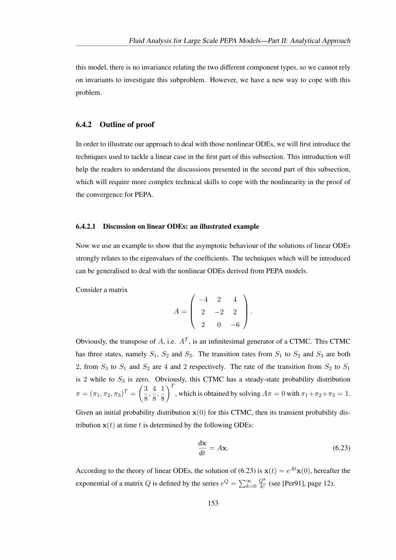
Fluid Analysis for Large Scale PEPA Models—Part II: Analytical Approach
this model, there is no invariance relating the two different component types, so we cannot rely
on invariants to investigate this subproblem. However, we have a new way to cope with this
problem.
6.4.2 Outline of proof
In order to illustrate our approach to deal with those nonlinear ODEs, we will first introduce the
techniques used to tackle a linear case in the first part of this subsection. This introduction will
help the readers to understand the discussions presented in the second part of this subsection,
which will require more complex technical skills to cope with the nonlinearity in the proof of
the convergence for PEPA.
6.4.2.1 Discussion on linear ODEs: an illustrated example
Now we use an example to show that the asymptotic behaviour of the solutions of linear ODEs
strongly relates to the eigenvalues of the coefficients. The techniques which will be introduced
can be generalised to deal with the nonlinear ODEs derived from PEPA models.
Consider a matrix
A =
−4 2 4
2 −2 2
2 0 −6
.
Obviously, the transpose of A, i.e. AT , is an infinitesimal generator of a CTMC. This CTMC
has three states, namely S1, S2 and S3. The transition rates from S1 to S2 and S3 are both
2, from S3 to S1 and S2 are 4 and 2 respectively. The rate of the transition from S2 to S1
is 2 while to S3 is zero. Obviously, this CTMC has a steady-state probability distribution
π = (π1, π2, π3)T =(
38,48,18
)T
, which is obtained by solving Aπ = 0 with π1+π2+π3 = 1.
Given an initial probability distribution x(0) for this CTMC, then its transient probability dis-
tribution x(t) at time t is determined by the following ODEs:
dxdt
= Ax. (6.23)
According to the theory of linear ODEs, the solution of (6.23) is x(t) = eAtx(0), hereafter the
exponential of a matrix Q is defined by the series eQ =∑∞
k=0Qk
k! (see [Per91], page 12).
153
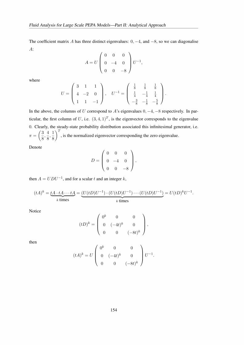
Fluid Analysis for Large Scale PEPA Models—Part II: Analytical Approach
The coefficient matrix A has three distinct eigenvalues: 0,−4, and −8, so we can diagonalise
A:
A = U
0 0 0
0 −4 0
0 0 −8
U−1,
where
U =
3 1 1
4 −2 0
1 1 −1
, U−1 =
18
18
18
14 −1
414
−38 −1
8 −58
.
In the above, the columns of U correspond to A’s eigenvalues 0,−4,−8 respectively. In par-
ticular, the first column of U , i.e. (3, 4, 1)T , is the eigenvector corresponds to the eigenvalue
0. Clearly, the steady-state probability distribution associated this infinitesimal generator, i.e.
π =(
38,48,18
)T
, is the normalized eigenvector corresponding the zero eigenvalue.
Denote
D =
0 0 0
0 −4 0
0 0 −8
,
then A = UDU−1, and for a scalar t and an integer k,
(tA)k = tA · tA · · · tA︸ ︷︷ ︸k times
= (U(tD)U−1) · (U(tD)U−1) · · · (U(tD)U−1)︸ ︷︷ ︸k times
= U(tD)kU−1.
Notice
(tD)k =
0k 0 0
0 (−4t)k 0
0 0 (−8t)k
,
then
(tA)k = U
0k 0 0
0 (−4t)k 0
0 0 (−8t)k
U−1.
154
Fluid Analysis for Large Scale PEPA Models—Part II: Analytical Approach
Noticing 0! = 00 = 1, so
∞∑k=0
1k!
0k 0 0
0 (−4t)k 0
0 0 (−8t)k
=
1 0 0
0∞∑
k=0
(−4t)k
k! 0
0 0∞∑
k=0
(−8t)k
k!
=
1 0 0
0 e−4t 0
0 0 e−8t
where the last equality holds is due to the Taylor expansion ey =∑∞
k=0yk
k! for any y. Therefore,
we have
etA =∞∑
k=0
(tA)k
k!
=∞∑
k=0
1k!
U
0k 0 0
0 (−4t)k 0
0 0 (−8t)k
U−1
= U
∞∑k=0
1k!
0k 0 0
0 (−4t)k 0
0 0 (−8t)k
U−1
= U
1 0 0
0 e−4t 0
0 0 e−8t
U−1.
So, given an initial value x(0), the solution of (6.23) is
x(t) = eAtx(0) = U
1 0 0
0 e−4t 0
0 0 e−8t
U−1x(0). (6.24)
As time goes to infinity, both e−4t and e−8t converge to zeros, thus x(t) converges to a constant
x∗, where
x∗ = U
1 0 0
0 0 0
0 0 0
U−1x(0). (6.25)
155
Fluid Analysis for Large Scale PEPA Models—Part II: Analytical Approach
With some calculation,
x∗ = U
1 0 0
0 0 0
0 0 0
U−1x(0)
= U
1
0
0
( 1 0 0)
U−1x(0)
=
3
4
1
( 18
18
18
)x1(0)
x2(0)
x3(0)
=
3(x1(0)+x2(0)+x3(0))
84(x1(0)+x2(0)+x3(0))
8x1(0)+x2(0)+x3(0)
8
.
(6.26)
Since x(0) = (x1(0), x2(0), x3(0))T is an initial probability distribution, so∑3
i=1 xi(0) = 1.
Thus, x∗ =(
38,48,18
), which coincides with the steady-state distribution π. From (6.26), we
can see that x∗ is determined by the first column of U and the first row of U−1. Since the first
row of U−1 only takes the role of normalisation, so the the steady-state distribution is ultimately
determined by the first column of U , i.e. the eigenvector corresponds to the eigenvalue zero.
In fact, from the equation Aπ = 0 = 0π, we also know that π is in fact an eigenvector
corresponding to the eigenvalue 0.
Moreover, the speed of the convergence to the steady-state distribution depends on the nonzero
eigenvalues of the generator. For example, it is easy to see that the convergence speed in our
case depends on e−4t and e−8t. Because e−8t ≤ e−4t, i.e. e−8t converges to zero more quickly
than e−4t, so the convergence speed mainly depends on e−4t, or the largest nonzero eigenvalue
λ = −4. The estimation of the largest nonzero eigenvalue (called the principle eigenvalue in
some literature) is a hot topic in the fields of Markov theory and functional analysis [Che05,
Wan05], since it has lots of applications, including determining the speed of converging to
equilibria. In our case, a mathematical statement for the dependence of the convergence speed
on the principle eigenvalue λ = −4 is
‖x(t)− x∗‖ ≤ Ce−4t. (6.27)
156
Fluid Analysis for Large Scale PEPA Models—Part II: Analytical Approach
where C is a constant.
Not all coefficient matrices can be diagonalised and not all their eigenvalues are real num-
bers. However, as long as the eigenvalues are either zeros or have negative real parts then the
convergence for bounded solutions can be guaranteed by Corollary D.2.3 in Appendix D.2.
Furthermore, the largest real part of the eigenvalues determines the convergence speed. That is,
if
Λ = inf{−<(λ) | λ is a nonzero eigenvalue of A} (6.28)
whereafter <(·) represents the real part of a complex number, then by Theorem D.2.2 in Ap-
pendix D.2, the converge speed depends on Λ, that is,
‖x(t)− x∗‖ ≤ C(t)e−Λt. (6.29)
Here C(t) is a polynomial function. We should point out that as time goes to infinity, the
asymptotic behaviour of the product of a polynomial and an exponential function can mainly
be determined by the exponential function. In particular, as in our case, if C(t) = C is a
constant then (6.29) becomes
‖x(t)− x∗‖ ≤ Ce−Λt. (6.30)
Of course, both (6.29) and (6.30) can imply
limt→∞
‖x(t)− x∗‖ = 0. (6.31)
Moreover, in the situation that the eigenvalues are unknown, but as long as the corresponding
Λ is proven to be positive, then we can claim that x converges according to (6.29) and (6.30).
6.4.2.2 Dealing with nonlinearity in PEPA
As we have mentioned in the previous subsection, all remaining work to determine the conver-
gence for our ODEs (6.20) or (6.21) is to ensure that the ODEs will finally become linear. For
157
Fluid Analysis for Large Scale PEPA Models—Part II: Analytical Approach
convenience, the ODEs (6.20) are presented again, see the following
dx1
dt= −amin{x1, y1}+ bx2
dx2
dt= amin{x1, y1} − bx2
dy1
dt= −amin{x1, y1}+ dy2
dy2
dt= amin{x1, y1} − dy2
(6.32)
Notice y1(t) ≤ N by the boundedness of solutions. If we can prove that after time T ,
x1(t) ≥ cM , where c > 0 is independent of M , we will get, provided cM > N ,
x1(t) ≥ cM > N ≥ y1(t), t ≥ T.
Therefore, the ODEs (6.32) will become linear after time T . We hope to use the techniques
discussed previously to prove this conclusion. Because the ODEs considered previously are
linear, the previous techniques have to be improved to deal with the nonlinearity in our case.
Let
α(t) =
min{x1(t),y1(t)}
x1(t) , x1(t) 6= 0,
1, x1(t) = 0,
then 0 ≤ α(t) ≤ 1. The ODEs associated with component type X can be rewritten as
dx1
dt= −aα(t)x1 + bx2,
dx2
dt= aα(t)x1 − bx2.
(6.33)
Let
A(t) =
−aα(t) b
aα(t) −b
, X(t) =
x1(t)
x2(t)
.
Then (6.33) can be written asdX(t)
dt= A(t)X(t). (6.34)
The solution of (6.34) is
X(t) = eR t0 A(s)dsX(0). (6.35)
Notice, if A(t) is a constant matrix A, then the solution eR t0 A(s)dsX(0) = eAtX(0) coincides
158
Fluid Analysis for Large Scale PEPA Models—Part II: Analytical Approach
with (6.24), which is in the linear situation.
Let B(t) =1t
∫ t
0A(s)ds, then
X(t) = eR t0 A(s)dsX(0) = etB(t)X(0), (6.36)
and
B(t) =1t
−a∫ t0 α(s)ds bt
a∫ t0 α(s)ds −bt
=
−aβ(t) b
aβ(t) −b
, (6.37)
where β(t) =
∫ t0 α(s)ds
t. Obviously, 0 ≤ β(t) ≤ 1 because 0 ≤ α(s) ≤ 1.
Similar to the diagonalisation of A in Section 6.4.2.1, the matrix B(t) can be diagonalised as
B(t) =
−aβ(t) b
aβ(t) −b
=
baβ(t)+b 1aβ(t)
aβ(t)+b −1
0 0
0 −(aβ(t) + b)
1 1aβ(t)
aβ(t)+b − baβ(t)+b
= U(t)
0 0
0 −(aβ(t) + b)
U−1(t),
(6.38)
where
U(t) =
baβ(t)+b 1aβ(t)
aβ(t)+b −1
, U−1(t) =
1 1aβ(t)
aβ(t)+b − baβ(t)+b
. (6.39)
In the formula (6.38), both 0 and −(aβ(t) + b) are B(t)’s eigenvalues, while the columns of
U(t) are the corresponding eigenvectors. In particular,(
b
aβ(t) + b,
aβ(t)aβ(t) + b
)T
, i.e. the first
column of U(t), is the eigenvector corresponding to the eigenvalue zero.
Analogously to (6.25), we define a function X(t) by
X(t) = U(t)
1 0
0 0
U−1(t)X(0). (6.40)
159
Fluid Analysis for Large Scale PEPA Models—Part II: Analytical Approach
By simple calculation,
X(t) = (x1(t), x2(t))T =(
bM
aβ(t) + b,
aβ(t)Maβ(t) + b
)T
. (6.41)
Obviously, X(t) is the normalised eigenvector corresponding the zero eigenvalue (at the time
t), analogous to the equilibrium x∗ in Section 6.4.2.1. Here the normalisaton is in terms of
the total population M of the component type X . We hope to see that X(t) embodies some
equilibrium meaning. In fact, we can analogously prove a conclusion: for X(t) and X(t)
defined as above, we have
limt→∞
‖X(t)− X(t)‖ = 0. (6.42)
A proof of (6.42), which relies on the explicit expression of U(t), is given in Appendix D.5.
This conclusion is also included in Proposition 6.4.2, which will be introduced later.
Now we discuss the benefit brought by this formula. In fact, by (6.42) the first entry of X(t)
approximates the first entry of X(t), i.e. x1(t) approximates x1(t) =bM
aβ(t) + b. Thus, for any
ε > 0, there exists T > 0 such that for any t ≥ T ,
x1(t) > x1(t)− ε =bM
aβ(t) + b− ε.
SincebM
a + b≤ bM
aβ(t) + b≤ M because 0 ≤ β(t) ≤ 1, so x1(t) >
bM
a + b− ε. Therefore, if
bM
a + b> N , then by the boundedness of y1(t), i.e. y1(t) ≤ N , we have
x1(t) >bM
a + b− ε > N ≥ y1(t),
as long as ε is small enough. This means that Q2 will dominate the system after time T . So we
have
Proposition 6.4.1. IfbM
a + b> N , then the solution of the ODEs (6.21) converges as time tends
to infinity.
Since the model is symmetric, this proposition has a symmetric version: ifdN
a + d> M , then
the solution of the ODEs also converges.
As we discussed, there are two key steps in the proof of Proposition 6.4.1. The first step is to
establish the approximation of x1(t) to x1(t), i.e. x1(t) ≈ x1(t). The second one is to give
160
Fluid Analysis for Large Scale PEPA Models—Part II: Analytical Approach
an estimation x1(t) ≥ cM . According to these two conclusions, we have x1(t) ≥ c′M where
c′ < c, and therefore can conclude that x1(t) ≥ c′M > N > y1(t) provided the condition
c′M > N . This is the main philosophy behind our proof for x1(t) > y1(t).
For the sake of generality, the proofs of these two conclusions should not rely on the explicit
expressions of the eigenvalues and eigenvectors of B(t). This is because for general PEPA
models with two component types and one synchronisation, these explicit expressions are not
always available. The following subsection will present our discussions about these steps, and
the proofs for the conclusions which do not rely on these explicit expressions.
6.4.3 Proofs not relying on explicit expressions
This subsection will divide into two parts. In the first part, we will give a lower bound for
the eigenvalues of the coefficient matrix B(t), based on which a proof of the approximation of
X(t) to X(t) is given. The second part will establish the estimation x1(t) ≥ cM . All proofs
in this subsection do not require knowledge of the explicit expressions of the eigenvalues and
eigenvectors of B(t).
For convenience, in this subsection we define
f(β) =
−aβ b
aβ −b
, (6.43)
where f is a matrix-valued function defined on R. Then the matrix
B(t) =
−aβ(t) b
aβ(t) −b
is in fact a composition of the functions of f(β) and β = β(t). That is, B(t) = f(β(t)), where
t ∈ [0,∞). The diagonalisation of f(β) can be written as
f(β) = g(β)
0 0
0 λ(β)
g−1(β),
where λ(β) is f(β)’s nonzero eigenvalue, and g(β) is a matrix whose columns are the eigen-
vectors of f(β). Here g−1(β) is the inverse of the matrix g(β). Notice that λ(β) is real, because
if λ(β) is complex then its conjugation must be an eigenvalue, which is contradicted by the fact
161
Fluid Analysis for Large Scale PEPA Models—Part II: Analytical Approach
that f(β) only has two eigenvalues, 0 and λ(β). The following discussions in this subsection
do not rely on the explicit expressions of λ(β), g(β) and g−1(β), although it is easy to see that
λ(β) = −aβ + b and
g(β) =
baβ+b 1aβ
aβ+b −1
, g−1(β) =
1 1aβ
aβ+b − baβ+b
.
6.4.3.1 X(t) approximates X(t)
In the following, we will give a lower bound for the nonzero eigenvalue of f(β), i.e. λ(β), and
based on this prove the approximation of A(t) to X(t) as time tends to infinity.
If β > 0, then the transpose of f(β), i.e. f(β)T , is an infinitesimal generator, and thus the
nonzero eigenvalue λ(β) has negative real part, i.e. <(λ(β)) < 0. If β = 0, then f(β) is
independent of β and becomes a nonnegative matrix, i.e. each entry of it is nonnegative. Based
on the Perron-Frobenious theorem which is presented in the next section, we can still have
<(λ(0)) < 0. Therefore, for any β, f(β)’s eigenvalue other than zero has negative real part.
This conclusion is stated in the following lemma.
Lemma 6.4.1. For any β ∈ [0, 1], <(λ(β)) < 0, where λ(β) is a nonzero eigenvalue of f(β).
The proof of Lemma 6.4.1 is presented in Appendix D.6. Lemma 6.4.1 can further lead to the
following
Lemma 6.4.2. Let
Λ1 = infβ∈[0,1]
{−<(λ(β)) | λ(β) is f(β)’s non-zero eigenvalue}, (6.44)
then Λ1 > 0.
Proof. By Lemma 6.4.1, −<(λ(β)) > 0 for any β ∈ [0, 1], so Λ1 ≥ 0. Suppose Λ1 = 0.
Because the eigenvalue λ(β) is a continuous function of the matrix f(β), where f(β) is also
continuous on [0, 1] with respect to β, so λ(β) is a continuous function of β on [0, 1]. This
is due to the fact that a composition of continuous functions is still continuous. Noticing <(·)
is also a continuous function, so −<(λ(β)) is continuous with respect to λ(β), and thus with
respect to β on [0, 1]. Since a continuous function on a closed interval can achieve its minimum
(see Theorem D.1.3 in Appendix D.1), there exists β0 ∈ [0, 1] such that −<(λ(β0)) achieves
162
Fluid Analysis for Large Scale PEPA Models—Part II: Analytical Approach
the minimum Λ1, i.e. −<(λ(β0)) = Λ1 = 0. This is contradicted to Lemma 6.4.1. Therefore,
Λ1 > 0.
For any t ∈ [0,∞), β(t) ∈ [0, 1]. Thus {β(t) | t ∈ [0,∞)} ⊆ [0, 1]. Noticing B(t) = f(β(t)),
therefore
{λ | λ is B(t)’s non-zero eigenvalue, t > 0}
={λ | λ is f(β(t))’s non-zero eigenvalue, t > 0}
⊆{λ | λ is f(β)’s non-zero eigenvalue;β ∈ [0, 1]}.
(6.45)
Thus,
Λ , inf{−<(λ) | λ is B(t)’s nonzero eigenvalue, t > 0}
≥ inf{−<(λ) | λ is f(β)’s non-zero eigenvalue;β ∈ [0, 1]} = Λ1.(6.46)
Because Λ1 > 0 by Lemma 6.4.2, so Λ > 0. That is,
Corollary 6.4.3. Let
Λ = inft≥0{−<(λ(t)) | λ(t) is B(t)’s non-zero eigenvalue},
then Λ > 0.
Based on this corollary, we can prove the approximation of X(t) to X(t).
Proposition 6.4.2. Let X(t) = (x1(t), x2(t))T = etB(t)X(0), i.e. the solution of (6.33). Let
X(t) be defined by (6.40), i.e.
X(t) =
x1(t)
x2(t)
= U(t)
1
0
U(t)−1
x1(0)
x2(0)
. (6.47)
Then limt→∞
‖X(t)− X(t)‖ = 0.
Proof. Notice that eigenvectors of a matrix are continuous functions of the matrix. Since g(β)
is composed of the eigenvectors of the matrix f(β) and f(β) is continuous on [0, 1] with respect
to β, therefore g(β) is continuous on [0, 1] with respect to β. Because the inverse of a matrix is a
continuous mapping, so g−1(β), i.e. the inverse of g(β), is continuous with respect to g(β), and
163
Fluid Analysis for Large Scale PEPA Models—Part II: Analytical Approach
therefore is continuous on [0, 1] with respect to β since g(β) is continuous on [0, 1]. Since any
continuous function is bounded on a compact set [0, 1] (see Theorem D.1.3 in Appendix D.1),
both g(β) and g−1(β) are bounded on [0, 1]. That is, there exists K > 0 such that ‖g(β)‖ ≤ K
and ‖g−1(β)‖ ≤ K for all β ∈ [0, 1]. Because
{U(t) | t ∈ [0,∞)} = {g(β(t)) | t ∈ [0,∞)} ⊆ {g(β) | β ∈ [0, 1]},
we have
supt≥0
‖U(t)‖ ≤ supβ∈[0,1]
‖g(β)‖ ≤ K.
Similarly, supt≥0
∥∥U−1(t)∥∥ ≤ K. Notice
X(t)− X(t) =etB(t)X(0)− U(t)
1 0
0 0
U(t)−1X(0)
=
U(t)
1 0
0 etλ(t)
U(t)−1 − U(t)
1 0
0 0
U(t)−1
X(0)
=U(t)
0 0
0 etλ(t)
U(t)−1X(0),
where λ(t) is B(t)’s nonzero eigenvalue. By a similar argument to λ(β), λ(t) is also real.
Therefore,
−λ(t) = <(−λ(t)) = −<(λ(t)) ≥ Λ > 0
or λ(t) ≤ −Λ < 0, where Λ is defined in Corollary 6.4.3. Then
‖X(t)− X(t)‖ =
∥∥∥∥∥∥U(t)
0 0
0 etλ(t)
U(t)−1X(0)
∥∥∥∥∥∥≤‖U(t)‖
∥∥∥∥∥∥ 0 0
0 etλ(t)
∥∥∥∥∥∥ ‖U(t)−1‖‖X(0)‖
≤K2‖X(0)‖etλ(t)
≤K2‖X(0)‖e−tΛ.
Here we have used the norm property: ‖AB‖ ≤ ‖A‖‖B‖. Since Λ > 0, we have
limt→∞
‖X(t)− X(t)‖ = 0.
164
Fluid Analysis for Large Scale PEPA Models—Part II: Analytical Approach
6.4.3.2 An lower-bound estimation on population in local derivatives
In the following, we will prove that there exists T , such that x1(t) ≥ cM for any t > T .
We first define a function
h(β) = (h1(β), h2(β))T = g(β)
1 0
0 0
g−1(β)
x1(0)
x2(0)
.
Clearly, we have X(t) = h(β(t)) and x1(t) = h1(β(t)). Since β(t) ∈ [0, 1] for all t, the
following proposition can imply x1(t) ≥ cM .
Proposition 6.4.3. There exists c > 0 such that
infβ∈[0,1]
h1(β) ≥ cM.
where M = x1(0) + x2(0), c is independent of M .
Proof. Without loss of generality, we assume M = 1. We will show infβ∈[0,1]
h1(β) = c > 0.
Since h1(β) is a continuous function of β which is due to the continuity of g(β) and g−1(β),
by Theorem D.1.3 in Appendix D.1, h1(β) can achieve its minimum on [0, 1]. That is, there
exists β0 ∈ [0, 1], such that
h1(β0) = infβ∈[0,1]
h1(β) = c.
Consider the matrix
f(β0) =
−aβ0 b
aβ0 −b
and a set of linear ODEs dz1
dt
dz2dt
= f(β0)
z1
z2
. (6.48)
The solution of (6.48), given an initial value Z(0) = X(0) = (x1(0), x2(0))T , is
Z(t) = etf(β0)X(0).
According to (6.38), f(β0) can be diagonalised as
f(β0) = g(β0)
0 0
0 λ(β0)
g−1(β0).
165
Fluid Analysis for Large Scale PEPA Models—Part II: Analytical Approach
where λ(β0) is the nonzero and real eigenvalue of f(β0). Similarly to (6.24) and the discussions
in Section 6.4.2.1,
Z(t) = etf(β0)X(0) = g(β0)
1 0
0 etλ(β0)
g(β0)−1
x1(0)
x2(0)
. (6.49)
Because λ(β0) < 0 by Lemma 6.4.1, so as time goes to infinity,
Z(t) = g(β0)
1 0
0 etλ(β0)
g(β0)−1
x1(0)
x2(0)
−→ g(β0)
1 0
0 0
g(β0)−1
x1(0)
x2(0)
= h(β0).
(6.50)
That is, limt→∞
Z(t) = h(β0). In the following, we discuss two possible cases: β0 > 0 and
β0 = 0.
If β0 > 0, then the transpose of the matrix f(β0), i.e. f(β0)T , is an infinitesimal genera-
tor of an irreducible CTMC, which has two states and the transition rates between these two
states are aβ0 and b respectively. Moreover, the transient distribution of this CTMC, de-
noted by Z(t) = (z1(t), z2(t))T , satisfies the ODEs (6.48). As time goes to infinity, the
transient distribution Z(t) converges to the unique steady-state probability distribution. Since
limt→∞
Z(t) = h(β0), therefore h(β0) = (h1(β0), h2(β0))T is the steady-state probability distri-
bution and thus h1(β0) > 0. So infβ∈[0,1] h1(β) = h1(β0) > 0.
If β0 = 0, then
f(β0) =
0 b
0 −b
.
Since limt→∞
Z(t) = h(β0), therefore(
dz1
dt,dz2
dt
)T
converges to zero. Letting time go to infinity
on the both sides of (6.48), we obtain the following equilibrium equations, 0
0
= f(β0)
h1(β0)
h2(β0)
. (6.51)
166
Fluid Analysis for Large Scale PEPA Models—Part II: Analytical Approach
By the conservation law, (h1(β0)+h2(β0))T = M = 1. Therefore, (h1(β0), h2(β0))T satisfies f(β0)(h1(β0), h2(β0))T = 0,
h1(β0) + h2(β0) = M = 1.(6.52)
Solving (6.52), we obtain the unique solution (h1(β0), h2(β0))T = (1, 0)T . Therefore, h1(β0)
is one, and thus infβ∈[0,1] h1(β) = h1(β0) > 0.
Remark 6.4.1. As β tends to 0,
f(β) =
−aβ b
aβ −b
−→ f(0) =
0 b
0 −b
.
Correspondingly, for the equilibrium h(β) = (h1(β), h2(β))T =(
bMaβ+b ,
aβMaβ+b
)Tsatisfying
f(β)h(β) = 0 and h1(β) + h2(β) = M , we have(
bMaβ+b ,
aβMaβ+b
)T→ (M, 0)T as β tends to
zero. From the explicit expression, i.e. h1(β) = bMaβ+b , the minimum and maximum of h1(β)
are bMa+b and M respectively, which correspond to the matrices f(1) and f(0) respectively. In
the context of the PEPA model, f(1) corresponds to a free subsystem and there is no synchro-
nisation effect on it, i.e. the subsystem of component type X is independent of Y . The matrix
f(0) reflects that the subsystem of X has been influenced by the subsystem of Y , i.e. the rates
of shared activities are determined by Y , that is, the term amin{x1, y1} has been replaced
by ay1. Therefore the exit rates from the local derivative X1 correspondingly become smaller
since now ay1 < ax1. In order to balance the flux, which is described by the equilibrium
equation, the population of X1 must increase. That is why the equilibrium h1(β) increases
as β decreases. In short, synchronisations can increase the populations in syncrhonised local
derivatives in the steady state.
As an application of the above facts, if h1(β0) > 0 for some β0 > 0, then we can claim that
h1(0) > 0 because h1(0) ≥ h1(β0) > 0.
Obviously, Proposition 6.4.3 has a corollary:
Corollary 6.4.4. There exists c > 0 such that for any t ∈ [0,∞), x1(t) ≥ cM.
Proposition 6.4.2 and Proposition 6.4.3 can lead to the following lemma.
Lemma 6.4.5. There exists c > 0, T > 0, such that x1(t) ≥ cM for all t ≥ T .
167
Fluid Analysis for Large Scale PEPA Models—Part II: Analytical Approach
Proof. By Proposition 6.4.3 or Corollary 6.4.4, there exists c1, T1 > 0 such that x1(t) ≥ c1M
for any t > T1. By Proposition 6.4.2, limt→∞ |x1(t) − x1(t)| = 0, which implies that for any
ε, there exists T2 > 0 such that for any t > T2, x1(t) > x1(t) − ε. Choose T2 > T1, then we
have
x1(t) > x1(t)− ε ≥ c1M − ε.
Therefore, there exist c, T > 0 such that such that x1(t) ≥ cM for all t > T .
Because x1(t) ≥ cM , provided cM > N we have x1(t) ≥ cM > N ≥ y1(t), i.e., the system
will finally become linear. In the following we will show how to apply our method to more
general cases.
6.5 Convergence For Two Component Types and One Synchroni-
sation (II): General Case
This section deals with such an arbitrary PEPA model which has two component types and one
synchronisation. The local action rates of the shared activity are not assumed to be the same.
The main result of this section is a convergence theorem: as long as the population of one
component type is sufficiently larger than the population of the other, then the solution of the
derived ODEs converges as time tends to infinity.
6.5.1 Features of coefficient matrix
We assume the component types to be X and Y . The component type X is assumed to have
local derivatives X1, X2, · · · , Xm, while Y has local derivatives Y1, Y2, · · · , Yn. We use xi(t)
to denote the population of X in Xi (i = 1, · · · ,m) at time t. Similarly, yj(t) denotes the
population of Y in Yj (j = 1, · · · , n) at time t. Without loss of generality, we assume the
synchronisation is associated with the local derivatives X1 and Y1, i.e. the nonlinear term in
the derived ODEs is min{rx1(t), sy1(t)} where r and s are some constants. In fact, if the
synchronisation is associated with Xi and Yj , by appropriately permuting their suffixes, i.e.
i → 1, i + 1 → 2, · · · , i− 1 → m, j → 1, j + 1 → 2, · · · , j − 1 → n, the synchronisation
will be associated with X1 and Y1. According to the mapping semantics presented in the
168
Fluid Analysis for Large Scale PEPA Models—Part II: Analytical Approach
previous chapter, the derived ODEs from this class of PEPA model are
dxdt
=∑
l
lf(x, l) (6.53)
where x = (x1(t), · · · , xm(t), y1(t), · · · , yn(t))T . For convenience, we denote
X(t) = (x1(t), x2(t), · · · , xm(t))T ,
Y (t) = (y1(t), y2(t), · · · , yn(t))T .
In (6.53) all terms are linear except for those containing “min{rx1(t), sy1(t)}”. Notice
min{rx1(t), sy1(t)} = I{rx1(t)≤sy1(t)}rx1(t) + I{rx1(t)>sy1(t)}sy1(t).
When rx1(t) ≤ sy1(t), which is indicated by I{rx1(t)≤sy1(t)} = 1 and I{rx1(t)>sy1(t)} = 0,
we can replace min{rx1(t), sy1(t)} by rx1(t) in (6.53). Then (6.53) becomes linear since all
nonlinear terms are replaced by linear terms rx1(t), so the ODEs have the following form, dXdt
dYdt
= Q1
X
Y
, (6.54)
where Q1 is a coefficient matrix. Similarly, if rx1(t) > sy1(t), min{rx1(t), sy1(t)} can be
replaced by sy1(t) in (6.53). Then (6.53) can become dXdt
dYdt
= Q2
X
Y
, (6.55)
where Q2 is another coefficient matrix corresponding to the case of rx1(t) > sy1(t).
In short, the derived ODEs (6.53) are just the following dXdt
dYdt
= I{rx1≤sy1}Q1
X
Y
+ I{rx1>sy1}Q2
X
Y
. (6.56)
The case discussed in the previous section is a special case of this kind of form. If the conditions
rx1(t) ≤ sy1(t) and rx1(t) > sy1(t) occur alternately, then the matrices Q1 and Q2 will
correspondingly alternately dominate the system, as Figure 6.6 illustrates.
169
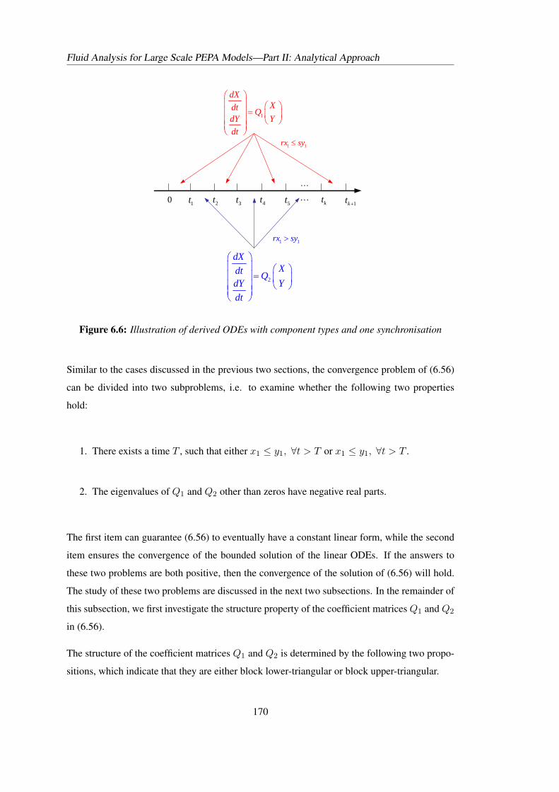
Fluid Analysis for Large Scale PEPA Models—Part II: Analytical Approach
0 1t 2t 3t kt4t 5t
1
dXXdt Q
dY Ydt
⎛ ⎞⎜ ⎟ ⎛ ⎞
=⎜ ⎟ ⎜ ⎟⎜ ⎟ ⎝ ⎠⎜ ⎟⎝ ⎠
1 1rx sy≤
2
dXXdt Q
dY Ydt
⎛ ⎞⎜ ⎟ ⎛ ⎞
=⎜ ⎟ ⎜ ⎟⎜ ⎟ ⎝ ⎠⎜ ⎟⎝ ⎠
1 1rx sy>
1kt +
Figure 6.6: Illustration of derived ODEs with component types and one synchronisation
Similar to the cases discussed in the previous two sections, the convergence problem of (6.56)
can be divided into two subproblems, i.e. to examine whether the following two properties
hold:
1. There exists a time T , such that either x1 ≤ y1, ∀t > T or x1 ≤ y1, ∀t > T .
2. The eigenvalues of Q1 and Q2 other than zeros have negative real parts.
The first item can guarantee (6.56) to eventually have a constant linear form, while the second
item ensures the convergence of the bounded solution of the linear ODEs. If the answers to
these two problems are both positive, then the convergence of the solution of (6.56) will hold.
The study of these two problems are discussed in the next two subsections. In the remainder of
this subsection, we first investigate the structure property of the coefficient matrices Q1 and Q2
in (6.56).
The structure of the coefficient matrices Q1 and Q2 is determined by the following two propo-
sitions, which indicate that they are either block lower-triangular or block upper-triangular.
170
Fluid Analysis for Large Scale PEPA Models—Part II: Analytical Approach
Proposition 6.5.1. Q1 in (6.56) can be written as
Q1 =
Q1 0
W Vn×n
(m+n)×(m+n)
, (6.57)
where QT1 is an infinitesimal generator matrix with the dimension m×m, and
Wn×m =
w11 0 · · · 0
w21 0 · · · 0...
......
...
wn1 0 · · · 0
, (6.58)
where w11 < 0, wj1(j = 2, · · · , n) ≥ 0 and∑n
j=1 wj1 = 0. Here V and W satisfy that if we
let
P = (W1 + V1, V2, · · · , Vn) , (6.59)
i.e. P ’s first column is the sum of V ’s first column and W ’s first column, while P ’s other
columns are the same to V ’s other columns, then P T is also an infinitesimal generator matrix.
Proof. Let
Q1 =
Q1 U
W V
, (6.60)
where Q1 and V are m×m and n× n matrices respectively. Suppose rx1(t) ≤ sy1(t), then dXdt
dYdt
= Q1
X
Y
=
Q1 U
W V
X
Y
. (6.61)
So we havedX
dt= Q1X + UY. (6.62)
The condition rx1(t) ≤ sy1(t) implies that all nonlinear terms min{rx1(t), sy1(t)} can be
replaced by x1(t). This means that the behaviour of the component type X in (6.61) and (6.62)
is independent of the component type Y . Thus in (6.61) U must be a zero matrix, i.e.
Q1 =
Q1 0
W V
.
171
Fluid Analysis for Large Scale PEPA Models—Part II: Analytical Approach
Moreover, (6.62) becomesdX
dt= Q1X, (6.63)
that is, there is no synchronisation in the ODEs corresponding to the component type X given
rx1(t) ≤ sy1(t). Then by Proposition 5.3.1 in Chapter 4, QT1 is an infinitesimal generator.
According to (6.61),
dY
dt= WX + V Y
= (W1,W2, · · · ,Wm)(x1, x2, · · · , xm)T + V Y
= x1W1 + V Y +m∑
i=2
xiWi,
(6.64)
where W = (W1,W2, · · · ,Wm). Notice that the component type Y is synchronised with
the component type X only through the term min{rx1(t), sy1(t)} = x1(t). In other words,
in (6.64) Y is directly dependent on only x1 other than xi (i ≥ 2). This implies W1 6= 0 while
Wi = 0 (i = 2, 3, · · · ,m). Therefore,
dY
dt= x1W1 + V Y
= x1W1 +n∑
j=1
yjVj ,(6.65)
where Vj (j = 1, 2, · · · , n) are the columns of V . Denote W1 = (w11, w21, · · · , wn1)T .
Notice that Y1 is a pre local derivative of the shared activity, and x1w11 represents the exit
rates of the shared activity from Y1. Therefore, w11 < 0. Moreover, x1wj1 (j = 2, · · · , n)
are the synchronised entry rates for the local derivatives Yj (j = 2, · · · , n) respectively, so
wj1 ≥ 0 (j = 2, · · · , n). By the conservation law, the total synchronised exit rates are equal to
the total synchronised entry rates, i.e. x1∑n
j=1 wj1 = 0 or∑n
j=1 wj1 = 0.
We have known that x1 in (6.65) derives from the synchronised term min{rx1, sy1}. If the
effect of the synchronisation on the behaviour of Y is removed, i.e. recover y1 by replacing x1,
172
Fluid Analysis for Large Scale PEPA Models—Part II: Analytical Approach
then (6.65) will become
dY
dt= y1W1 + V Y
= y1W1 +n∑
j=1
yjVj
= PY,
(6.66)
where P = (W1 + V1, V2, · · · , Vn). Since there is no synchronisation contained in the subsys-
tem of the component type Y , according to Proposition 5.3.1 in Chapter 4, P T is the infinitesi-
mal generator.
Similarly, we can prove
Proposition 6.5.2. Q2 in (6.56) can be written as
Q2 =
Em×m F
0 Q2
(m+n)×(m+n)
, (6.67)
where QT2 is an infinitesimal generator matrix with the dimension n× n, and
Fm×n =
f11 0 · · · 0
f21 0 · · · 0...
......
...
fm1 0 · · · 0
, (6.68)
where f11 < 0, fj1(j = 2, · · · ,m) ≥ 0 and∑m
j=1 fj1 = 0. Here F and E satisfy that if we let
R = (F1 + E1, E2, · · · , En) , (6.69)
then RT is also an infinitesimal generator matrix.
6.5.2 Eigenvalues of Q1 and Q2
In this subsection, we will determine the eigenvalue property of Q1 and Q2. First, the Perron-
Frobenius theorem gives an estimation of eigenvalues for nonnegative matrices.
Theorem 6.5.1. (Perron-Frobenius). Let A = (aij) be a real n × n matrix with nonnegative
173
Fluid Analysis for Large Scale PEPA Models—Part II: Analytical Approach
entries aij ≥ 0. Then the following statements hold:
1. There is a real eigenvalue r of A such that any other eigenvalue λ satisfies |λ| ≤ r.
2. r satisfies mini
∑j aij ≤ r ≤ max
i
∑j aij .
Remark 6.5.1. We should point out that in the second property, exchanging i and j in aij in the
formula, we still have mini
∑j aji ≤ r ≤ max
i
∑j aji. In fact, AT is also a real matrix with
non-negative entries. Since AT and A share the same eigenvalues, so r is one of the eigenvalues
of AT , such that any other eigenvalue λ of AT satisfies |λ| ≤ r. Notice (AT )ij = Aji, By
applying the Perron-Frobenius theorem to AT , we have
mini
∑j
aji ≤ r ≤ maxi
∑j
aji.
We cannot directly apply this theorem to our coefficient matrices Q1 and Q2, since both of
them have negative elements, not only on the diagonal but also in other entries. However, we
use some well-known techniques in linear algebra, i.e. the following Lemma 6.5.2 and 6.5.3
(which can be easily found in linear algebra textbooks), to cope with this problem, and thus
derive estimates of their eigenvalues.
Lemma 6.5.2. If Em×m and Fn×n have eigenvalues λi (i = 1, 2, · · · ,m) and δj
(j = 1, 2, · · · , n) respectively, then
H =
E 0
G F
has eigenvalues λi (i = 1, 2, · · · ,m) and δj (j = 1, 2, · · · , n).
Proof. Since E and F are square matrices, then by classical linear algebra theory,
|λI(m+n)×(m+n) −H| =
∣∣∣∣∣∣λI(m+n)×(m+n) −
E 0
G F
∣∣∣∣∣∣=
∣∣∣∣∣∣ λIm×m − E 0
−G λIn×n − F
∣∣∣∣∣∣= |λIm×m − E| × |λIn×n − F |,
174
Fluid Analysis for Large Scale PEPA Models—Part II: Analytical Approach
which implies
|λI(m+n)×(m+n) −H| = 0 ⇐⇒ |λIm×m − E| = 0 or |λIn×n − F | = 0.
In other words, E’s and F ’s eigenvalues are H’s eigenvalues, each eigenvalue of H is an
eigenvalue of either E or F .
Remark 6.5.2. This lemma is also valid for a block upper-triangular matrix,
H =
E G
0 F
.
The benefit of the lemma, in terms of eigenvalues, is to avoid caring about G, the lower-left or
upper-right block of H .
Lemma 6.5.2 shows that the eigenvalues of a block lower-triangular or block upper-triangular
matrix are only determined by the diagonal blocks. For example, the following two matrices −a b
a −b
,
0 d
0 −d
have eigenvalues 0,−(a + b) and 0,−d respectively. Notice
Q1 =
−a b 0 0
a −b 0 0
−a 0 0 d
a 0 0 −d
has eigenvalues 0 (two folds),−d,−(a + b). This is consistent with Lemma 6.5.2.
Lemma 6.5.3. If λ is an eigenvalue of V , then λ + r is an eigenvalue of V + rI , where r is a
scalar.
Proof. Let x be the eigenvector corresponding to λ, then
(V + rI)x = V x + rx = λx + rx = (λ + r)x.
So λ + r is an eigenvalue of V + rI .
175
Fluid Analysis for Large Scale PEPA Models—Part II: Analytical Approach
Remark 6.5.3. If some diagonal elements of V are negative, by adding such a matrix rI where
r is large enough, all the diagonal elements can become positive or nonnegative. Meanwhile,
all eigenvalues simply have an r-shift.
Theorem 6.5.4. The eigenvalues of both Q1 and Q2 are either zeros or have negative real
parts.
Proof. We only give the proof for Q1’s case. By Proposition 6.5.1,
Q1 =
Q1 0
W Vn×n
(m+n)×(m+n)
. (6.70)
According to Lemma 6.5.2, if all eigenvalues of Q1 and V are determined, then the eigenvalues
of Q1 will be determined. Let us consider V first.
Notice that only diagonal elements of V are possibly negative (which can be deduced from
Proposition 6.5.1). Let r = supi|Vii| > 0, then all the entries of V + rI are nonnegative. Let λ
be an arbitrary eigenvalue of V , then by Lemma 6.5.3, λ + r is an eigenvalue of V + rI .
Notice the sum of the elements of any column of V is zero (because the sum of entry rates
equals to the sum of exit rates), so V has a zero eigenvalue with the corresponding eigenvector
1, i.e. V 1 = 0. Thus r = 0 + r is an eigenvalue of V + rI . Moreover,
mini
∑j
(V + rI)ji = r = maxi
∑j
(V + rI)ji.
Applying the Perron-Frobenius theorem (Theorem 6.5.1) and Remark 6.5.1 to V + rI , so
|λ + r| ≤ r. (6.71)
Let λ = a + bi, then (6.71) implies that a ≤ 0, and if a = 0 then b = 0. In other words, V ’s
eigenvalues are either zeros or have negative real parts.
Similarly, Q1’s eigenvalues other than zeros have negative real parts. By Lemma 6.5.2, the
eigenvalues of Q1 other than zeros have negative real parts. The proof is complete.
176
Fluid Analysis for Large Scale PEPA Models—Part II: Analytical Approach
6.5.3 Convergence theorem
Now we deal with another subproblem: whether or not after a long time, we always have
rx1 ≥ sy1 (or rx1 < sy1). If the population of X is significantly larger than the population of
Y , intuitively, there will finally be a greater number of X in the local derivative X1, than the
number of Y in Y1. This will lead to rx1 > sy1.
Lemma 6.5.5. Under the assumptions in Section 6.4.1, for the following ODEs dXdt
dYdt
= I{rx1≤sy1}Q1
X
Y
+ I{rx1>sy1}Q2
X
Y
,
there exists c1 > 0, c2 > 0, T > 0, such that x1(t) ≥ c1M , y1(t) ≥ c2N for any t ≥ T , where
c1 and c2 are independent of M and N .
Proof. The proof is essentially the same as the proof of Lemma 6.4.5. We only give the sketch
of the proof for x1(t) ≥ c1M . By introducing new two functions α(t) and β(t),
α(t) =
min{rx1(t),sy1(t)}
rx1(t) , x1(t) 6= 0,
0, x1(t) = 0.,
β(t) =1t
∫ t
0α(s)ds,
the nonlinear term min{rx1(t), sy1(t)} equals rα(t)x1(t), and thus the ODEs associated with
the subsystem X can be written asdX
dt= A(t)X (6.72)
where A(t) is related to α(t). The solution of (6.72) is X(t) = etB(t)X(0), where B(t) is
defined by B(t) =1t
∫ t
0A(s)ds, and thus B(t) is related to β(t).
Notice that according to Theorem 6.5.4 and its proof, the eigenvalues of B(t) other than zeros
have negative real parts for any t > 0. By a similar proof to Corollary 6.4.3, we have
Λ = inft≥0{−<(λ) | λ is B(t)’s non-zero eigenvalue} > 0. (6.73)
This fact will lead to the conclusion that X(t) can be approximated by X(t), where X(t) is
constructed similarly to the one in Proposition 6.4.2. Because a general B(t) considered here
may not be diagonalisable, so the construction of X(t) is a little bit more complicated. We
177

Fluid Analysis for Large Scale PEPA Models—Part II: Analytical Approach
detail the construction as well as the proof of the following result in Appendix D.2.2:
limt→∞
‖X(t)− X(t)‖ = 0.
Then, by similar arguments to Proposition 6.4.3 and Corollary 6.4.4, we can prove that
inft>T x1(t) ≥ cM , where x1(t) is the first entry of X(t). Then, by a similar proof to the
proof of Lemma 6.4.5, we can conclude that there exists a number c1 such that x1(t) ≥ c1M
after a time T .
Lemma 6.5.6. Under the assumptions of Lemma 6.5.5, if M > K1N or N > K2M , where
constants K1 > 0 and K2 > 0 are sufficiently large, then there exists T such that
rx1(t) ≥ sy1(t), ∀t ≥ T or rx1(t) ≤ sy1(t), ∀t ≥ T respectively.
Proof. By the boundedness of solutions, 0 ≤ x1(t) ≤ M and 0 ≤ y1(t) ≤ N for any t.
Suppose M > K1N . By Lemma 6.5.5, there exists c, T > 0, x1(t) ≥ cM, ∀t ≥ T . Since K1
is assumed to be large enough such that K1 ≥ src , then rcM > sN . So for any t > T , we have
rx1(t) ≥ rcM ≥ sN ≥ sy1(t).
If N > K2M , the proof is similar and omitted here.
Now we state our convergence theorem.
Theorem 6.5.7. If M > K1N or N > K2M , where constants K1,K2 > 0 are sufficiently
large, then the solution of the derived ODEs (6.56), i.e. dXdt
dYdt
= I{rx1≤sy1}Q1
X
Y
+ I{rx1>sy1}Q2
X
Y
,
converges to a finite limit as time goes to infinity.
Proof. Suppose M > K1N , then by Lemma 6.5.6, there exists a time T > 0, such that after
time T , rx1(t) ≥ sy1(t), so (6.56) becomes dXdt
dYdt
= Q2
X
Y
. (6.74)
178
Fluid Analysis for Large Scale PEPA Models—Part II: Analytical Approach
Since Q2’s eigenvalues other than zeros have strict negative real parts according to Theo-
rem 6.5.4, and the solution of the above equation is bounded, then by Corollary D.2.3, the
solution converges to a finite limit as time goes to infinity.
Remark 6.5.4. We should point out that for a general PEPA model with two component types
and one synchronisation, the limit of the solution of the derived ODEs is determined by the
populations of these two component types rather than the particular starting state. That is to
say, whatever the initial state is, as long as the total populations of the components are the
same, the limit that the solution converges to will always be the same. We do not plan to discuss
this topic in detail in this thesis.
6.6 Summary
In this chapter, we have presented our investigations in the fluid approximation for PEPA, from
an analytical perspective. The analytical proofs for the convergence of the solutions of the
ODEs derived from some PEPA models, have been demonstrated. In particular, the case study
of an interesting model, i.e. Model 3, has shown that the structural property of invariance can be
used to prove the convergence. Moreover, for the class of models with two component types and
one synchronisation, the converge has been proved under some mild conditions. In addition,
this chapter has also presented an analytical proof for the boundedness of the solutions for any
general PEPA model.
179

180
Chapter 7
Deriving Performance Measures forLarge Scale Content Adaptation
Systems
7.1 Introduction
In the previous chapters, we have presented the techniques and theoretical results developed for
the PEPA language. This chapter will show how to derive performance measures from large
scale PEPA models based on the previous developments, as well as demonstrate the application
of these developments to large scale content adaptation systems proposed by the Mobile VCE.
In this chapter, numerical experiments are used to show the properties of the fluid approxima-
tion of the content adaptation PEPA model, with an emphasis on the convergence and consis-
tence characteristics. Then, we will discuss what kind of performance measures can be derived
through this fluid approximation approach. In order to obtain the performance metrics that can-
not be derived through this approach, we propose a Gillespie stochastic simulation algorithm
based on our numerical representation scheme of PEPA. Elaborated comparisons of the dif-
ferent approaches for deriving performance measures from content adaptation systems will be
subsequently presented.
Finally, for the purpose of demonstrating the performance derivation and evaluation for large
scale PEPA models through the fluid approximation approach, this chapter will detail the nu-
merical solutions of the ODEs derived from the content adaptation model, assessing the sen-
sitivity of the framework to the performance of individual components, and the scalability of
the framework under increasing loads and different resource conditions. Structural analysis of
a content adaptation system, in terms of invariance analysis and deadlock-checking for a sub-
system, as an application of the techniques developed in Chapter 4, is also briefly discussed in
this chapter.
181
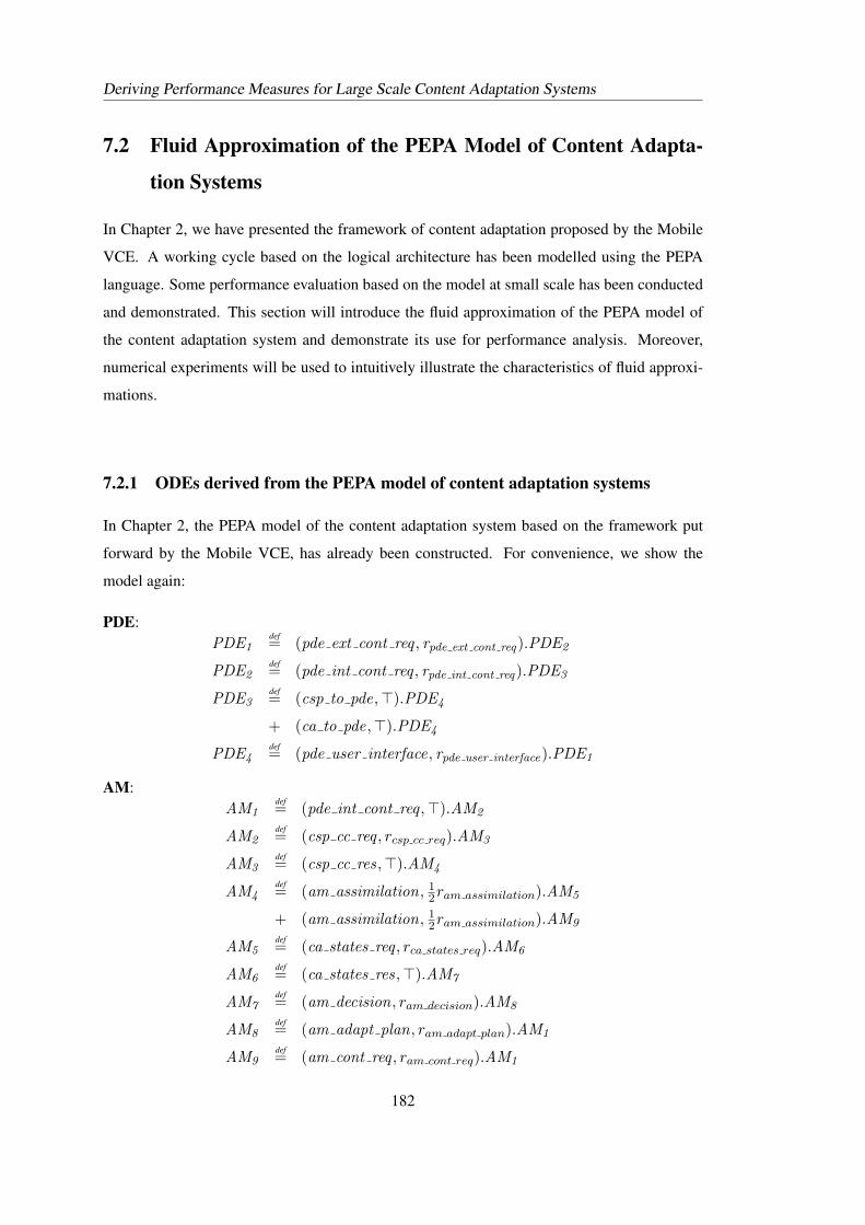
Deriving Performance Measures for Large Scale Content Adaptation Systems
7.2 Fluid Approximation of the PEPA Model of Content Adapta-
tion Systems
In Chapter 2, we have presented the framework of content adaptation proposed by the Mobile
VCE. A working cycle based on the logical architecture has been modelled using the PEPA
language. Some performance evaluation based on the model at small scale has been conducted
and demonstrated. This section will introduce the fluid approximation of the PEPA model of
the content adaptation system and demonstrate its use for performance analysis. Moreover,
numerical experiments will be used to intuitively illustrate the characteristics of fluid approxi-
mations.
7.2.1 ODEs derived from the PEPA model of content adaptation systems
In Chapter 2, the PEPA model of the content adaptation system based on the framework put
forward by the Mobile VCE, has already been constructed. For convenience, we show the
model again:
PDE:PDE1
def= (pde ext cont req , rpde ext cont req).PDE2
PDE2def= (pde int cont req , rpde int cont req).PDE3
PDE3def= (csp to pde,>).PDE4
+ (ca to pde,>).PDE4
PDE4def= (pde user interface, rpde user interface).PDE1
AM:AM1
def= (pde int cont req ,>).AM2
AM2def= (csp cc req , rcsp cc req).AM3
AM3def= (csp cc res,>).AM4
AM4def= (am assimilation, 1
2ram assimilation).AM5
+ (am assimilation, 12ram assimilation).AM9
AM5def= (ca states req , rca states req).AM6
AM6def= (ca states res,>).AM7
AM7def= (am decision, ram decision).AM8
AM8def= (am adapt plan, ram adapt plan).AM1
AM9def= (am cont req , ram cont req).AM1
182
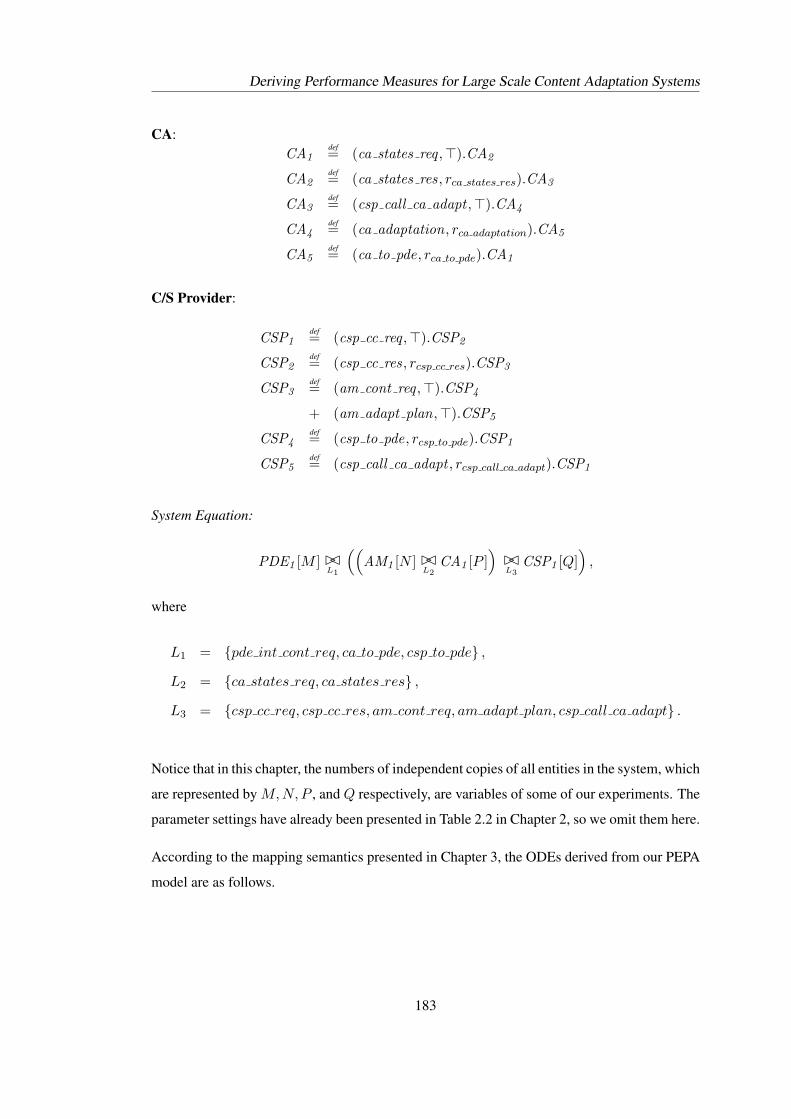
Deriving Performance Measures for Large Scale Content Adaptation Systems
CA:CA1
def= (ca states req ,>).CA2
CA2def= (ca states res, rca states res).CA3
CA3def= (csp call ca adapt ,>).CA4
CA4def= (ca adaptation, rca adaptation).CA5
CA5def= (ca to pde, rca to pde).CA1
C/S Provider:
CSP1def= (csp cc req ,>).CSP2
CSP2def= (csp cc res, rcsp cc res).CSP3
CSP3def= (am cont req ,>).CSP4
+ (am adapt plan,>).CSP5
CSP4def= (csp to pde, rcsp to pde).CSP1
CSP5def= (csp call ca adapt , rcsp call ca adapt).CSP1
System Equation:
PDE1 [M ] BCL1
((AM1 [N ] BC
L2CA1 [P ]
)BCL3
CSP1 [Q])
,
where
L1 = {pde int cont req, ca to pde, csp to pde} ,
L2 = {ca states req, ca states res} ,
L3 = {csp cc req, csp cc res, am cont req, am adapt plan, csp call ca adapt} .
Notice that in this chapter, the numbers of independent copies of all entities in the system, which
are represented by M,N,P , and Q respectively, are variables of some of our experiments. The
parameter settings have already been presented in Table 2.2 in Chapter 2, so we omit them here.
According to the mapping semantics presented in Chapter 3, the ODEs derived from our PEPA
model are as follows.
183
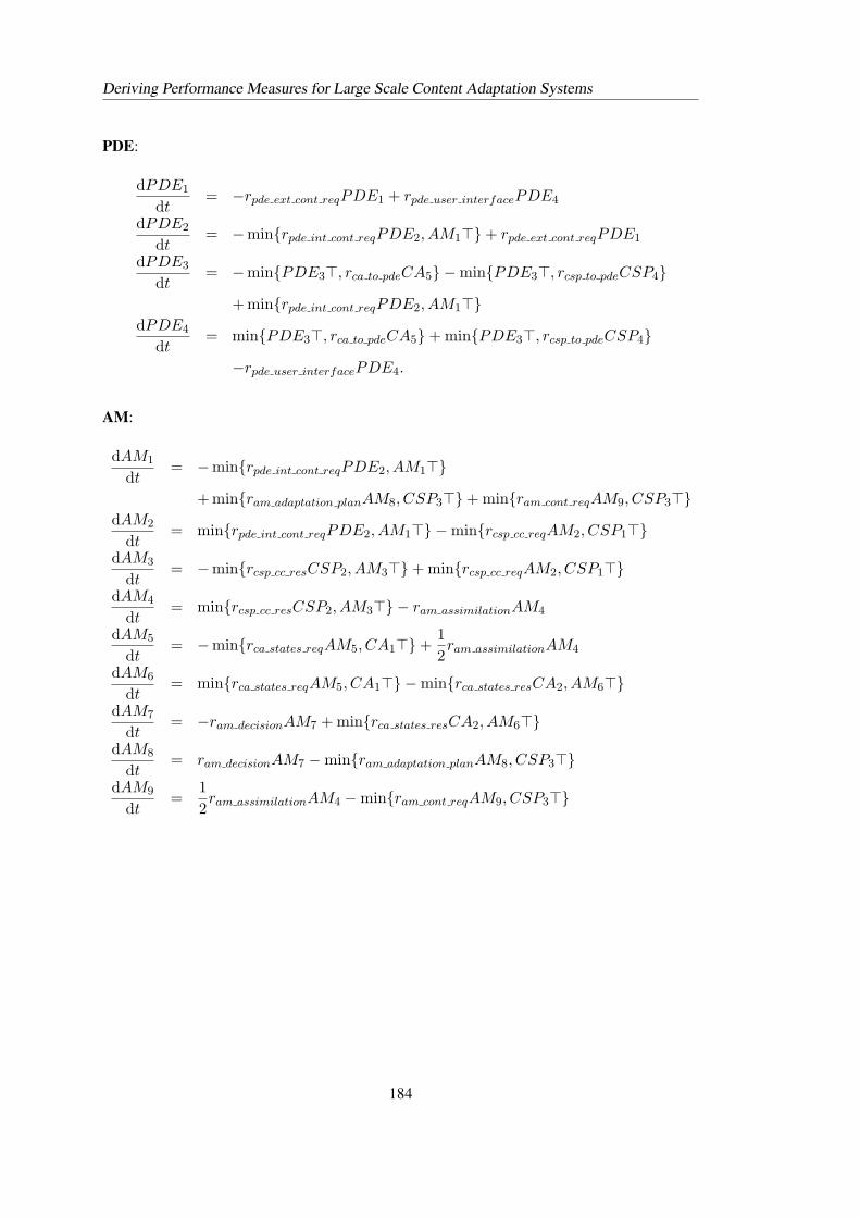
Deriving Performance Measures for Large Scale Content Adaptation Systems
PDE:
dPDE1
dt= −rpde ext cont reqPDE1 + rpde user interfacePDE4
dPDE2
dt= −min{rpde int cont reqPDE2, AM1>}+ rpde ext cont reqPDE1
dPDE3
dt= −min{PDE3>, rca to pdeCA5} −min{PDE3>, rcsp to pdeCSP4}
+min{rpde int cont reqPDE2, AM1>}dPDE4
dt= min{PDE3>, rca to pdeCA5}+ min{PDE3>, rcsp to pdeCSP4}
−rpde user interfacePDE4.
AM:
dAM1
dt= −min{rpde int cont reqPDE2, AM1>}
+min{ram adaptation planAM8, CSP3>}+ min{ram cont reqAM9, CSP3>}dAM2
dt= min{rpde int cont reqPDE2, AM1>} −min{rcsp cc reqAM2, CSP1>}
dAM3
dt= −min{rcsp cc resCSP2, AM3>}+ min{rcsp cc reqAM2, CSP1>}
dAM4
dt= min{rcsp cc resCSP2, AM3>} − ram assimilationAM4
dAM5
dt= −min{rca states reqAM5, CA1>}+
12ram assimilationAM4
dAM6
dt= min{rca states reqAM5, CA1>} −min{rca states resCA2, AM6>}
dAM7
dt= −ram decisionAM7 + min{rca states resCA2, AM6>}
dAM8
dt= ram decisionAM7 −min{ram adaptation planAM8, CSP3>}
dAM9
dt=
12ram assimilationAM4 −min{ram cont reqAM9, CSP3>}
184
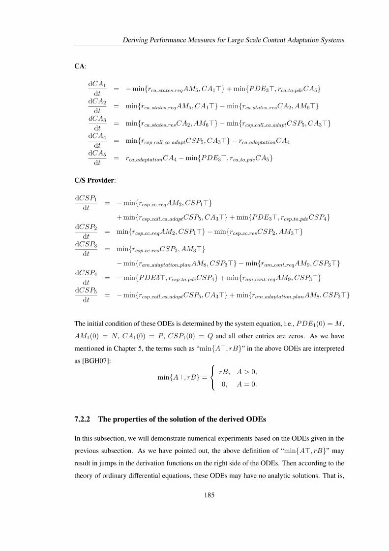
Deriving Performance Measures for Large Scale Content Adaptation Systems
CA:
dCA1
dt= −min{rca states reqAM5, CA1>}+ min{PDE3>, rca to pdeCA5}
dCA2
dt= min{rca states reqAM5, CA1>} −min{rca states resCA2, AM6>}
dCA3
dt= min{rca states resCA2, AM6>} −min{rcsp call ca adaptCSP5, CA3>}
dCA4
dt= min{rcsp call ca adaptCSP5, CA3>} − rca adaptationCA4
dCA5
dt= rca adaptationCA4 −min{PDE3>, rca to pdeCA5}
C/S Provider:
dCSP1
dt= −min{rcsp cc reqAM2, CSP1>}
+min{rcsp call ca adaptCSP5, CA3>}+ min{PDE3>, rcsp to pdeCSP4}dCSP2
dt= min{rcsp cc reqAM2, CSP1>} −min{rcsp cc resCSP2, AM3>}
dCSP3
dt= min{rcsp cc resCSP2, AM3>}
−min{ram adaptation planAM8, CSP3>} −min{ram cont reqAM9, CSP3>}dCSP4
dt= −min{PDE3>, rcsp to pdeCSP4}+ min{ram cont reqAM9, CSP3>}
dCSP5
dt= −min{rcsp call ca adaptCSP5, CA3>}+ min{ram adaptation planAM8, CSP3>}
The initial condition of these ODEs is determined by the system equation, i.e., PDE1(0) = M ,
AM1(0) = N , CA1(0) = P , CSP1(0) = Q and all other entries are zeros. As we have
mentioned in Chapter 5, the terms such as “min{A>, rB}” in the above ODEs are interpreted
as [BGH07]:
min{A>, rB} =
rB, A > 0,
0, A = 0.
7.2.2 The properties of the solution of the derived ODEs
In this subsection, we will demonstrate numerical experiments based on the ODEs given in the
previous subsection. As we have pointed out, the above definition of “min{A>, rB}” may
result in jumps in the derivation functions on the right side of the ODEs. Then according to the
theory of ordinary differential equations, these ODEs may have no analytic solutions. That is,
185
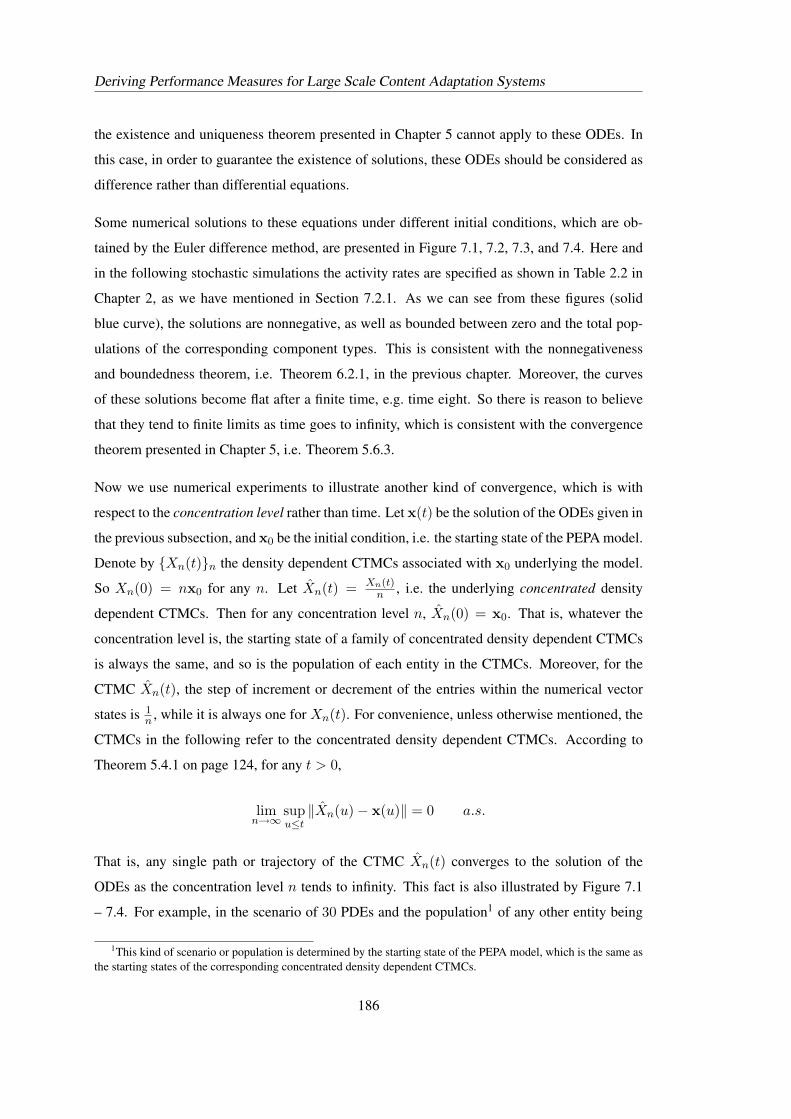
Deriving Performance Measures for Large Scale Content Adaptation Systems
the existence and uniqueness theorem presented in Chapter 5 cannot apply to these ODEs. In
this case, in order to guarantee the existence of solutions, these ODEs should be considered as
difference rather than differential equations.
Some numerical solutions to these equations under different initial conditions, which are ob-
tained by the Euler difference method, are presented in Figure 7.1, 7.2, 7.3, and 7.4. Here and
in the following stochastic simulations the activity rates are specified as shown in Table 2.2 in
Chapter 2, as we have mentioned in Section 7.2.1. As we can see from these figures (solid
blue curve), the solutions are nonnegative, as well as bounded between zero and the total pop-
ulations of the corresponding component types. This is consistent with the nonnegativeness
and boundedness theorem, i.e. Theorem 6.2.1, in the previous chapter. Moreover, the curves
of these solutions become flat after a finite time, e.g. time eight. So there is reason to believe
that they tend to finite limits as time goes to infinity, which is consistent with the convergence
theorem presented in Chapter 5, i.e. Theorem 5.6.3.
Now we use numerical experiments to illustrate another kind of convergence, which is with
respect to the concentration level rather than time. Let x(t) be the solution of the ODEs given in
the previous subsection, and x0 be the initial condition, i.e. the starting state of the PEPA model.
Denote by {Xn(t)}n the density dependent CTMCs associated with x0 underlying the model.
So Xn(0) = nx0 for any n. Let Xn(t) = Xn(t)n , i.e. the underlying concentrated density
dependent CTMCs. Then for any concentration level n, Xn(0) = x0. That is, whatever the
concentration level is, the starting state of a family of concentrated density dependent CTMCs
is always the same, and so is the population of each entity in the CTMCs. Moreover, for the
CTMC Xn(t), the step of increment or decrement of the entries within the numerical vector
states is 1n , while it is always one for Xn(t). For convenience, unless otherwise mentioned, the
CTMCs in the following refer to the concentrated density dependent CTMCs. According to
Theorem 5.4.1 on page 124, for any t > 0,
limn→∞
supu≤t
‖Xn(u)− x(u)‖ = 0 a.s.
That is, any single path or trajectory of the CTMC Xn(t) converges to the solution of the
ODEs as the concentration level n tends to infinity. This fact is also illustrated by Figure 7.1
– 7.4. For example, in the scenario of 30 PDEs and the population1 of any other entity being
1This kind of scenario or population is determined by the starting state of the PEPA model, which is the same asthe starting states of the corresponding concentrated density dependent CTMCs.
186
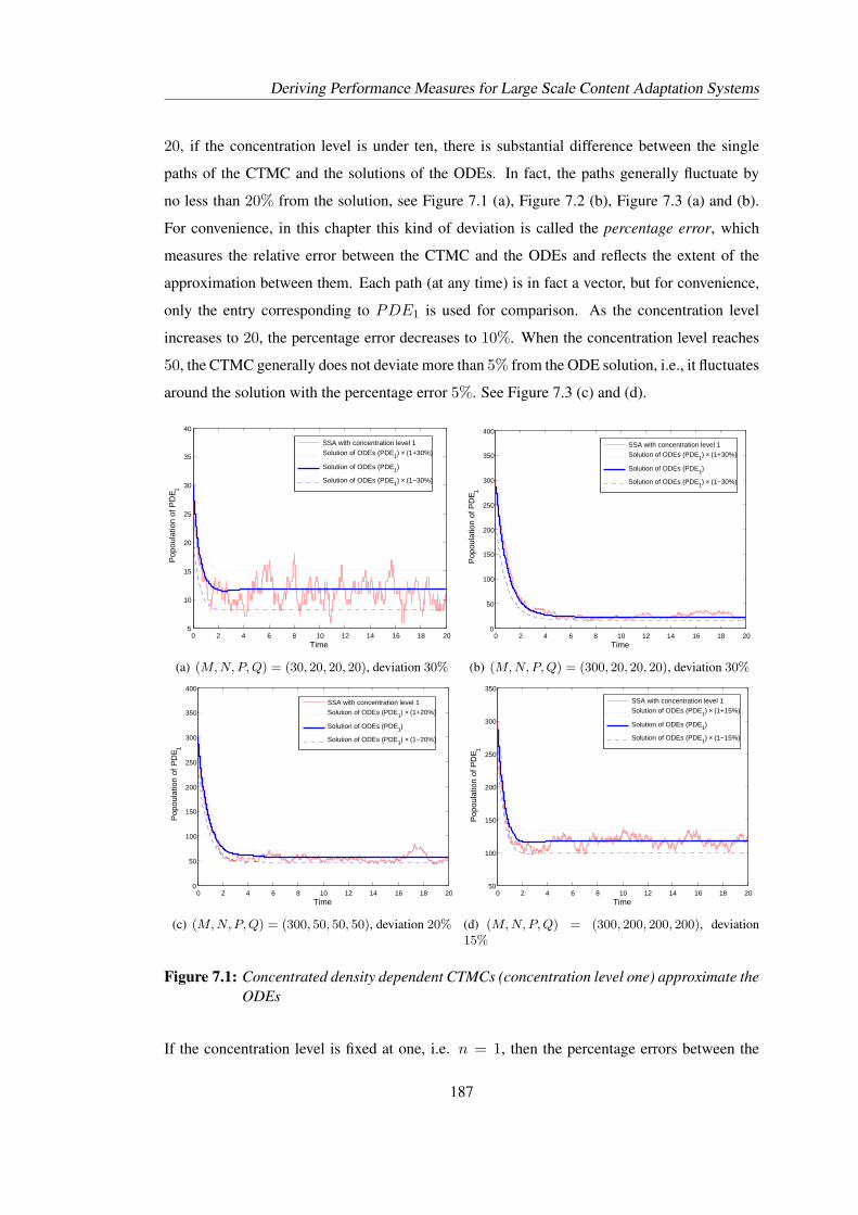
Deriving Performance Measures for Large Scale Content Adaptation Systems
20, if the concentration level is under ten, there is substantial difference between the single
paths of the CTMC and the solutions of the ODEs. In fact, the paths generally fluctuate by
no less than 20% from the solution, see Figure 7.1 (a), Figure 7.2 (b), Figure 7.3 (a) and (b).
For convenience, in this chapter this kind of deviation is called the percentage error, which
measures the relative error between the CTMC and the ODEs and reflects the extent of the
approximation between them. Each path (at any time) is in fact a vector, but for convenience,
only the entry corresponding to PDE1 is used for comparison. As the concentration level
increases to 20, the percentage error decreases to 10%. When the concentration level reaches
50, the CTMC generally does not deviate more than 5% from the ODE solution, i.e., it fluctuates
around the solution with the percentage error 5%. See Figure 7.3 (c) and (d).
0 2 4 6 8 10 12 14 16 18 205
10
15
20
25
30
35
40
Pop
oula
tion
of P
DE 1
Time
SSA with concentration level 1Solution of ODEs (PDE1) × (1+30%)
Solution of ODEs (PDE1)
Solution of ODEs (PDE1) × (1−30%)
(a) (M, N, P, Q) = (30, 20, 20, 20), deviation 30%
0 2 4 6 8 10 12 14 16 18 200
50
100
150
200
250
300
350
400
Pop
oula
tion
of P
DE 1
Time
SSA with concentration level 1Solution of ODEs (PDE1) × (1+30%)
Solution of ODEs (PDE1)
Solution of ODEs (PDE1) × (1−30%)
(b) (M, N, P, Q) = (300, 20, 20, 20), deviation 30%
0 2 4 6 8 10 12 14 16 18 200
50
100
150
200
250
300
350
400
Pop
oula
tion
of P
DE 1
Time
SSA with concentration level 1Solution of ODEs (PDE1) × (1+20%)
Solution of ODEs (PDE1)
Solution of ODEs (PDE1) × (1−20%)
(c) (M, N, P, Q) = (300, 50, 50, 50), deviation 20%
0 2 4 6 8 10 12 14 16 18 2050
100
150
200
250
300
350
Pop
oula
tion
of P
DE 1
Time
SSA with concentration level 1Solution of ODEs (PDE1) × (1+15%)
Solution of ODEs (PDE1)
Solution of ODEs (PDE1) × (1−15%)
(d) (M, N, P, Q) = (300, 200, 200, 200), deviation15%
Figure 7.1: Concentrated density dependent CTMCs (concentration level one) approximate theODEs
If the concentration level is fixed at one, i.e. n = 1, then the percentage errors between the
187
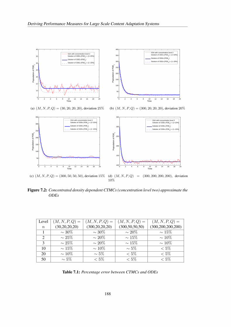
Deriving Performance Measures for Large Scale Content Adaptation Systems
0 2 4 6 8 10 12 14 16 18 205
10
15
20
25
30
35
40
Pop
oula
tion
of P
DE
1
Time
SSA with concentration level 2Solution of ODEs (PDE
1) × (1+25%)
Solution of ODEs (PDE1)
Solution of ODEs (PDE1) × (1−25%)
(a) (M, N, P, Q) = (30, 20, 20, 20), deviation 25%
0 2 4 6 8 10 12 14 16 18 200
50
100
150
200
250
300
350
400
Pop
oula
tion
of P
DE
1
Time
SSA with concentration level 2Solution of ODEs (PDE
1) × (1+20%)
Solution of ODEs (PDE1)
Solution of ODEs (PDE1) × (1−20%)
(b) (M, N, P, Q) = (300, 20, 20, 20), deviation 20%
0 2 4 6 8 10 12 14 16 18 200
50
100
150
200
250
300
350
Pop
oula
tion
of P
DE
1
Time
SSA with concentration level 2Solution of ODEs (PDE
1) × (1+15%)
Solution of ODEs (PDE1)
Solution of ODEs (PDE1) × (1−15%)
(c) (M, N, P, Q) = (300, 50, 50, 50), deviation 15%
0 2 4 6 8 10 12 14 16 18 20100
150
200
250
300
350
Pop
oula
tion
of P
DE
1
Time
SSA with concentration level 2Solution of ODEs (PDE
1) × (1+10%)
Solution of ODEs (PDE1)
Solution of ODEs (PDE1) × (1−10%)
(d) (M, N, P, Q) = (300, 200, 200, 200), deviation10%
Figure 7.2: Concentrated density dependent CTMCs (concentration level two) approximate theODEs
Level (M,N,P, Q) = (M,N,P, Q) = (M,N,P, Q) = (M,N,P, Q) =n (30,20,20,20) (300,20,20,20) (300,50,50,50) (300,200,200,200)1 ∼ 30% ∼ 30% ∼ 20% ∼ 15%2 ∼ 25% ∼ 20% ∼ 15% ∼ 10%3 ∼ 25% ∼ 20% ∼ 15% ∼ 10%10 ∼ 15% ∼ 10% ∼ 5% < 5%20 ∼ 10% ∼ 5% < 5% < 5%50 ∼ 5% < 5% < 5% < 5%
Table 7.1: Percentage error between CTMCs and ODEs
188
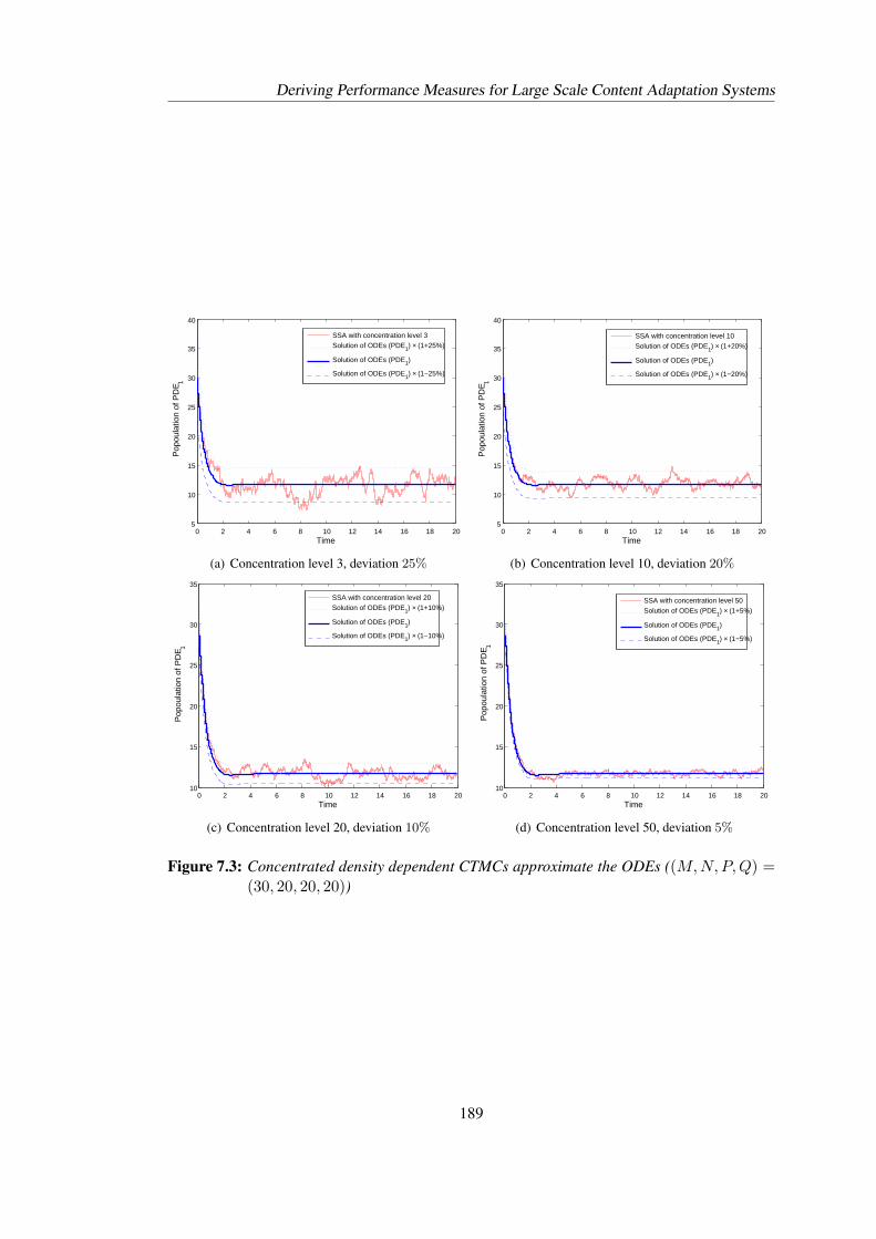
Deriving Performance Measures for Large Scale Content Adaptation Systems
0 2 4 6 8 10 12 14 16 18 205
10
15
20
25
30
35
40
Pop
oula
tion
of P
DE 1
Time
SSA with concentration level 3Solution of ODEs (PDE1) × (1+25%)
Solution of ODEs (PDE1)
Solution of ODEs (PDE1) × (1−25%)
(a) Concentration level 3, deviation 25%
0 2 4 6 8 10 12 14 16 18 205
10
15
20
25
30
35
40
Pop
oula
tion
of P
DE 1
Time
SSA with concentration level 10Solution of ODEs (PDE1) × (1+20%)
Solution of ODEs (PDE1)
Solution of ODEs (PDE1) × (1−20%)
(b) Concentration level 10, deviation 20%
0 2 4 6 8 10 12 14 16 18 2010
15
20
25
30
35
Pop
oula
tion
of P
DE 1
Time
SSA with concentration level 20Solution of ODEs (PDE1) × (1+10%)
Solution of ODEs (PDE1)
Solution of ODEs (PDE1) × (1−10%)
(c) Concentration level 20, deviation 10%
0 2 4 6 8 10 12 14 16 18 2010
15
20
25
30
35
Pop
oula
tion
of P
DE 1
Time
SSA with concentration level 50Solution of ODEs (PDE1) × (1+5%)
Solution of ODEs (PDE1)
Solution of ODEs (PDE1) × (1−5%)
(d) Concentration level 50, deviation 5%
Figure 7.3: Concentrated density dependent CTMCs approximate the ODEs ((M,N,P, Q) =(30, 20, 20, 20))
189
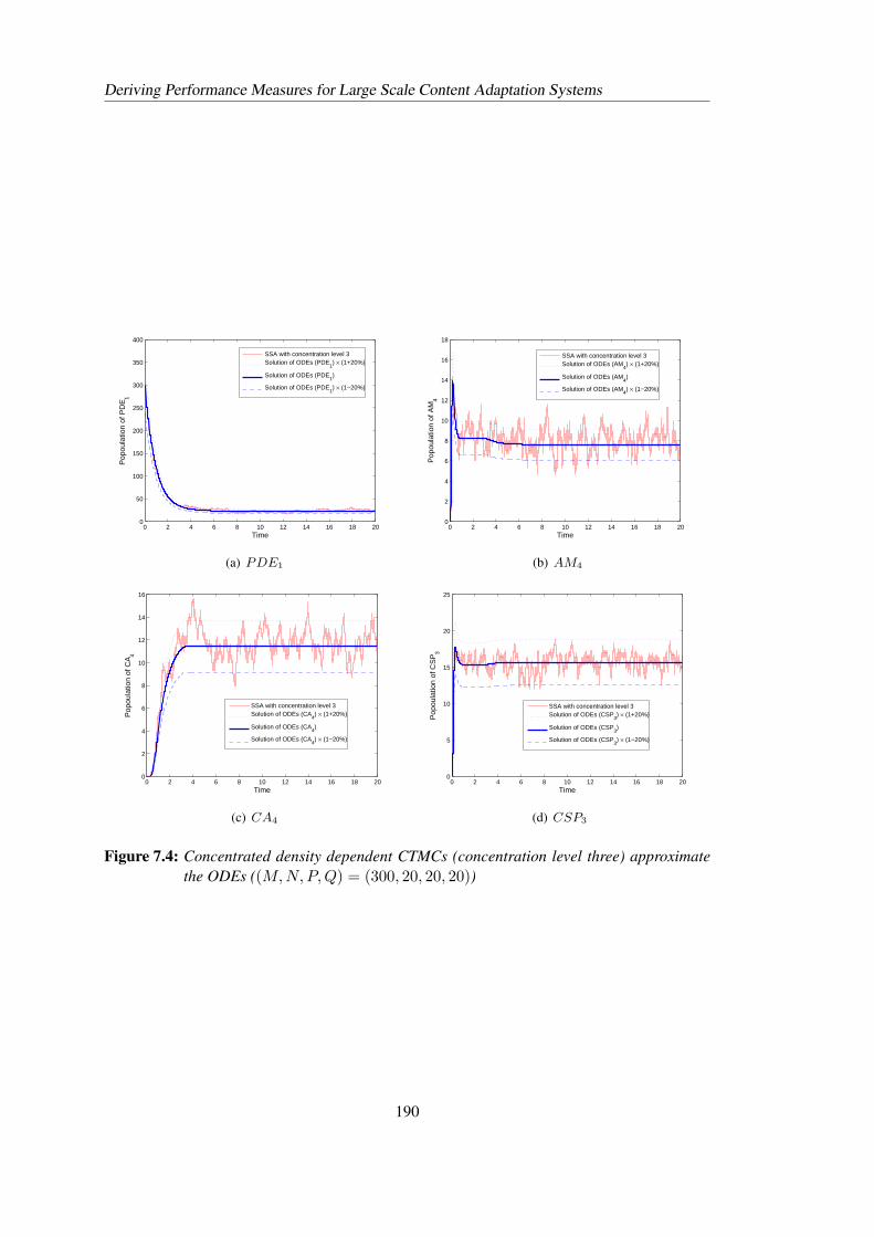
Deriving Performance Measures for Large Scale Content Adaptation Systems
0 2 4 6 8 10 12 14 16 18 200
50
100
150
200
250
300
350
400
Pop
oula
tion
of P
DE
1
Time
SSA with concentration level 3Solution of ODEs (PDE
1) × (1+20%)
Solution of ODEs (PDE1)
Solution of ODEs (PDE1) × (1−20%)
(a) PDE1
0 2 4 6 8 10 12 14 16 18 200
2
4
6
8
10
12
14
16
18
Pop
oula
tion
of A
M4
Time
SSA with concentration level 3Solution of ODEs (AM
4) × (1+20%)
Solution of ODEs (AM4)
Solution of ODEs (AM4) × (1−20%)
(b) AM4
0 2 4 6 8 10 12 14 16 18 200
2
4
6
8
10
12
14
16
Pop
oula
tion
of C
A4
Time
SSA with concentration level 3Solution of ODEs (CA
4) × (1+20%)
Solution of ODEs (CA4)
Solution of ODEs (CA4) × (1−20%)
(c) CA4
0 2 4 6 8 10 12 14 16 18 200
5
10
15
20
25
Pop
oula
tion
of C
SP
3
Time
SSA with concentration level 3Solution of ODEs (CSP
3) × (1+20%)
Solution of ODEs (CSP3)
Solution of ODEs (CSP3) × (1−20%)
(d) CSP3
Figure 7.4: Concentrated density dependent CTMCs (concentration level three) approximatethe ODEs ((M,N,P, Q) = (300, 20, 20, 20))
190
Deriving Performance Measures for Large Scale Content Adaptation Systems
paths and the solutions are about 30%, when there are 30 and 300 PDEs in the system while
the population of each other entity is fixed at 20. See Figure 7.1 (a) and Figure 7.1 (b). That
is, there is not much difference with respect to deviation between the cases of 30 PDEs and
300 PDEs in that scenario. But when n = 2, in the same scenario, the percentage errors are
obviously different since these errors are 25% and 20% respectively, see Figure 7.2 (a) and
Figure 7.2 (b). When the population of each other entity increases to 50 and further to 200
while the number of PDEs is fixed at 300, then the percentage errors significantly decrease
regardless of whether n = 1 or n = 2, see Figure 7.1 (c) and (d), as well as Figure 7.2 (c)
and (d). That is, the population size on the server side (N,P, Q) has a significant effect on the
approximation accuracy. Moreover, these suggest that the smallest population of the entities has
more effect on percentage errors than the maximum of the populations has. This observation
can be supported by further experimental results that are presented in Table 7.1 (on page 188).
In this table, M,N,P, Q represent the numbers of PDE1, AM1, CA1 and CSP1 in the starting
state. As illustrated by this table, as the population increases (both in terms of the smallest and
maximum of the populations), the level needed to achieve percentage error of approximately
5% or less will decrease.
The evolution of the populations of some other entities, such as AM4, CA4 and CSP3, in the
scenario (M,N,P, Q) = (300, 20, 20, 20), has been demonstrated in Figure 7.4. These entities
have a similar percentage error to the one of PDE1.
We should point out that the percentage error discussed here is in terms of the difference be-
tween one-realisation (i.e. one run) of the CTMC and the solution of the ODEs. There is
no doubt that, the “averaged path” in each figure should have much smaller deviations. This
phenomenon can be theoretically explained. For example, let {ξi}ni=1 be a family of random
variables and each of them has the same variance, namely σ2. Then the average of {ξi}ni=1, i.e.
1n
∑ni=1 ξi has a reduced variance σ2
n , provided that these random variables are independent.
An averaged path can be considered as the average of multiple trajectories of the CTMC, which
therefore should have a reduced variance. Thus, the concentration level needed to achieve a
percentage error with respect to average path should be smaller than the error with respect to
single path.
191
Deriving Performance Measures for Large Scale Content Adaptation Systems
7.3 Deriving Quantitative Performance Measures through Differ-
ent Approaches
In Section 2.4 of Chapter 2, we have discussed how to derive performance measures from small
scale PEPA models, through the approach of solving global balance, linear algebraic equations.
This approach is not feasible for large scale models due to the state-space explosion problem.
However, we have alternative ways to obtain quantitative performance measures from a large
scale PEPA model, which will be discussed in this section.
7.3.1 Deriving performance measures through fluid approximation approach
In this subsection, we will discuss what kind of performance measures can be derived through
the fluid approximation approach and how these performance measures can be derived from
PEPA models. As illustrated in Chapter 5, for a given PEPA model, there is a family of density
dependent CTMCs, namely, Xn(t), underlying this model. Let Xn(t) be the concentrated
density dependent CTMCs, i.e. Xn(t) = Xn(t)n . Denote the expectation of Xn(t) by Mn(t),
that is,
Mn(t) = E[Xn(t)] =∑s∈Sn
sπnt (s),
where Sn and πnt (·) are the state space and the transient probability distribution of Xn(t),
respectively. Letdxdt
= F (x) =∑
l∈Alabel
lf(x, l)
be the ODEs derived from this model. Then according to Lemma 5.5.1 in Chapter 5,
limn→∞
Mn(t) = limn→∞
E[Xn(t)] = x(t). (7.1)
Moreover, as Theorem 5.6.3 states, under the stated condition, the solution x(t) of the ODEs
converges to a limit x∗ as time tends to infinity, and satisfies
limt→∞
limn→∞
Mn(t) = limt→∞
x(t) = x∗. (7.2)
That is,
limt→∞
limn→∞
E[Xn(t)] = x∗. (7.3)
192
Deriving Performance Measures for Large Scale Content Adaptation Systems
According to (7.1) and (7.3), the fluid approximation of a PEPA model captures the information
of the first-order moments of the underlying CTMCs. Correspondingly, from the perspective
of performance measure, all performance metrics that only depend on the first-order moment
information can be derived through this fluid approximation approach. These metrics include:
the throughput of an acitivity, utilisation, average response time. However, if a performance
metric needs or relates the information of higher-order moments, then this approach may not
be sufficient to derive this performance. In the following, we will mathematically discuss this
problem.
For the CTMC Xn(t) given above, some averaged transient performance measure ξ(n, t) can
be expressed by
ξ(n, t) = E[ρ(Xn(t))] =∑s∈Sn
ρ(s)πnt (s),
where ρ is a reward function. Some discussions about reward functions have been presented in
Chapter 2. If ρ is a linear function, then this performance measure can be derived through the
fluid approximation approach. See the following proposition.
Proposition 7.3.1. For a given PEPA model, let {Xn(t)}n be the family of concentrated density
dependent CTMCs underlying this model. Let x(t) be the solution of the ODEs derived from
this model. Then for ξ(n, t) = E[ρ(Xn(t))], where ρ is a linear function, we have
limn→∞
E[ρ(Xn(t))] = ρ(x(t)). (7.4)
Moreover, if limt→∞
x(t) = x∗, then
limt→∞
limn→∞
E[ρ(Xn(t))] = ρ(x∗). (7.5)
Proof. Because ρ is linear, so we can exchange the notations of the expectation and the function
ρ (Proposition 2.4, [BZ99]), that is E[ρ(·)] = ρ(E[·]). Therefore,
limn→∞
E[ρ(Xn(t))] = limn→∞
ρ(E[Xn(t)]).
Since ρ is linear and thus continuous, so limn→∞
ρ(E[Xn(t)]) = ρ( limn→∞
E[Xn(t)]). Then by
(7.1), limn→∞
E[Xn(t)] = x(t), so we have limn→∞E[ρ(Xn(t))] = ρ(x(t)), which completes
the first assertion.
193
Deriving Performance Measures for Large Scale Content Adaptation Systems
Moreover, if limt→∞
x(t) = x∗, we have
limt→∞
limn→∞
ξ(n, t) = limt→∞
limn→∞
E[ρ(Xn(t))]
= limt→∞
limn→∞
ρ(E[Xn(t)])
= ρ(
limt→∞
limn→∞
E[Xn(t)])
= ρ(
limt→∞
x(t))
= ρ(x∗).
In above formula, the second “=” holds because E[ρ(·)] = ρ(E[·]) for a linear function ρ. The
third “=” holds due to the continuity of ρ.
We should point out that if ρ is not a linear function, then Proposition 7.3.1 may not hold.
This is because, for a general function, we may not have the property E[ρ(·)] = ρ(E[·])
which is needed in the proof of Proposition 7.3.1. In fact, if ρ is a convex function, then
E[ρ(·)] ≥ ρ(E[·]) (Theorem 2.2 (Jensen’s inequality) [BZ99]), so both (7.4) and (7.5) may
not hold. However, in this case we can still benefit from the fluid approximation: the value
calculated from the ODEs gives an upper bound on the performance measure. As we have
mentioned, the convergence theorem, i.e. Theorem 5.6.3, captures the information of the first-
order moments of the CTMCs. A linear mapping of the first-order is still first-order, and this
first-order information can be provided by the ODEs. That is why a performance measure that
can be defined through a linear reward function, can be derived through the fluid approximation.
As we have discussed in Chapter 2, many performance measures of interest can be repre-
sented through a linear reward function. For example, the average throughput of the activ-
ity ca adaptation in the CTMC Xn(t) underlying the content adaptation model, denoted by
Thr(ca adaptation, n, t), is
Thr(ca adaptation, n, t) =∑s∈Sn
(s[CA4]rca adaptation) πnt (s), (7.6)
where s[CA4] indicates the population of CA4 in the state s. Let ρ1(s) = s[CA4]rca adaptation,
then
Thr(ca adaptation, n, t) = E[ρ1(Xn(t))]. (7.7)
194
Deriving Performance Measures for Large Scale Content Adaptation Systems
Since ρ1(s) is linear with respect to s, we can conclude that
limt→∞
limn→∞
Thr(ca adaptation, n, t) = x∗[CA1]rca adaptationdef= Thr∗(ca adaptation).
(7.8)
Here Thr∗(ca adaptation) reflects the throughput of ca adaptation in the equilibrium state,
i.e. the limit of the transient throughput as time as well as the concentration level tends to
infinity.
In addition to the throughput of activities, utilisation can also be derived through the fluid
approximation approach. For example, the utilisation of the idle state CA1 is defined as
Util(CA1, n, t) =∑s∈Sn
(s[CA1]NCA
)πn
t (s), (7.9)
where NCA is the total population of the component CA. Similarly, if we let ρ2(s) = s[CA1]NCA
,
then ρ2 is linear and
Util(CA1, n, t) = E[ρ2(Xn(t))]. (7.10)
According to Proposition 7.3.1,
limt→∞
limn→∞
Util(CA1, n, t) =x∗[CA1]
NCA
def= Util∗(CA1). (7.11)
Unfortunately, this approach cannot be used to derive the measure of “variation of the utilisation
of CA1”, which is defined by
∑s∈S
(s[CA1]NCA
− x∗[CA1]NCA
)2
π(s).
This is because information about the second-order moment such as∑
s∈S (s[CA1])2 π(s) is
needed in this metric but the ODEs cannot provide this information. That is to say, not all
rewards associated with the CTMCs underlying PEPA models can be derived through the fluid
approximation approach, only those that depend on the first-order moments of the CTMCs.
We should point out that some work on the fluid approximation of higher-order moments of
the component counting stochastic processes for a PEPA model has been presented in [HB08],
but there is no theoretical justification. In [HB09], the application of fluid-generated higher
moments to passage-time approximations has been demonstrated.
195
Deriving Performance Measures for Large Scale Content Adaptation Systems
To conclude, if a performance metric is population-based, or can be represented by a linear
reward function, then this measure can be derived through the fluid approximation approach.
Otherwise, it is not possible to derive this metric using this approach. However, in this situation,
we still have methods to get this measure from PEPA models, which will be presented later in
this chapter. In the following, we first discuss how to use Little’s law to derive average response
time.
7.3.2 Deriving average response time via Little’s Law
Response time is a very important performance metric which has already been discussed based
on a small scale system in Chapter 2. For large scale systems, a good method to get average
response time through fluid approximation models has been demonstrated in [CDGH08]. In
that paper, expected passage response times for large PEPA models are calculated using Little’s
law.
Little’s Law [Lit61] is usually phrased in terms of the jobs in a system and relates the average
number of jobs in the system N to the residence time W , the average time they spend in the
system. Let X be the throughput, i.e. the number of jobs completed during a unit time. Then
for the system in its steady-state, Little’s law states that:
N = XW
The residence time, of course, is the response time if we take the system to be that which occurs
between a request and response action within a model. The only requirement for using Little’s
law is the existence of a stationary state.
For the content adaptation model, what we want to measure is the duration of the service flows,
i.e. the time from the starting activity pde int cont req to the ending activity csp to pde or
ca to pde. Then using Little’s Law we obtain:
W =PDE∗
2 + PDE∗3
PDE∗1 × rpde ext cont req
, (7.12)
where PDE∗i represents the population of the local derivative PDEi in the steady state
(i = 1, 2, 3). In (7.12), the sum of PDE∗2 and PDE∗
3 represents the number of jobs engaged in
the service in the system and PDE∗1 × rpde ext cont req is the corresponding throughput. Since
196
Deriving Performance Measures for Large Scale Content Adaptation Systems
in the steady state the rates of flux in and out are equal, so PDE∗1 × rpde ext cont req in (7.12)
could equally be replaced with PDE∗4 × rpde user interface, where PDE∗
4 is the population of
PDE4 in the steady state.
To get the average response time W , the only remaining work is to determine the values of
PDE∗i (i = 1, 2, 3). Clearly, PDE∗
i (i = 1, 2, 3) are three entries of the vector of the
equilibrium solution x∗ of the ODEs derived from the same model. Therefore, the average
response time is available as long as the solution is available. It should be pointed out that the
steady solution x∗ can be directly derived from the equilibrium equation:
F (x∗) =∑
l∈Alabel
lf(x∗, l) = 0. (7.13)
In fact, since limt→∞
x(t) = x∗, then
0 = limt→∞
dxdt
= limt→∞
F (x) = F ( limt→∞
x) = F (x∗).
Therefore, the average response time is “approximately” governed by the equilibrium equation.
Thus in the sense of approximation, some capacity planning and optimisation for large scale
content adaptation systems can be simply and directly carried out based on a set of nonlinear
algebra equations.
7.3.3 Deriving performance measures through stochastic simulation approach
As discussed in Section 7.3.1, if a reward function associated with the CTMC underlying a
PEPA model is not linear, then we cannot derive the corresponding reward through the fluid
approximation approach. An alternative widely-used way to obtained performance is stochastic
simulation. In fact, Gillespie’s stochastic simulation algorithm (SSA) [Gil76] has already been
implemented in the PEPA Eclipse plug-in [TDG09], a tool supporting PEPA.
The Gillespie algorithm has been widely applied to model and simulate biochemical reac-
tions [Kie02]. This method exploits the fact that the duration from one transition (or reaction)
to the next satisfies an exponential distribution with the reciprocal of total transition rate as
the mean, and assumes that the transition rate is dependent on the state [UHCW06]. In the
context of PEPA, this algorithm can be directly constructed based on our numerical represen-
197
Deriving Performance Measures for Large Scale Content Adaptation Systems
tation scheme that is defined in Chapter 3, see Algorithm 3. In Algorithm 3, the states of a
PEPA model are represented as numerical vector forms, and the rates between those states are
specified by the transition rate functions which only depend on the transition type (i.e. labelled
activity) and the current state. In this algorithm, the generated time τ in each iteration can be
regarded as having been drawn from an exponential distribution with the mean1
f(x), which
has already been pointed out in [Gil76]. Therefore, Line 9 in Algorithm 3 is in fact expressing:
“generate τ from an exponential distribution with the mean1
f(x)”.
Thus, this algorithm is essentially to simulate the CTMC underlying a PEPA model.
We have several reasons to put forward this algorithm in this thesis. Firstly, as one benefit of
our numerical representation scheme, it provides a good platform for directly and conveniently
exploiting the simulation algorithm for PEPA. Secondly, we emphasise that any general perfor-
mance measure can be derived from PEPA models through this kind of simulation, particularly
those that cannot be obtained by the fluid approximation approach. In addition, the simulated
results can be used for comparisons with those obtained by solving ODEs. Finally, simulations
offer a new insight into the dynamics of the CTMCs underlying PEPA models from the stochas-
tic perspective, which is in contrast to the deterministic fluid approximation approach discussed
intensively in the previous chapters.
In Algorithm 3, the stop condition could be: t > T , where T is a given large time. In addi-
tion, since the output performance converges as time goes to infinity as the following Propo-
sition 7.3.2 states, other choices for stopping the algorithm include: the absolute error of two
continued iterations is small enough:
δ =∣∣∣∣PerMeasuren
tn− PerMeasuren−1
tn−1
∣∣∣∣ < ε,
or the relative error is sufficient small:
δ
PerMeasuren/tn< ε,
where ε is a given small number, tn−1, tn are the accumulated time up to the n− 1-th and n-th
iterations respectively, while PerMeasuren−1 and PerMeasuren are the accumulated perfor-
mance up to the n− 1-th and n-th iterations respectively.
2In practise, in order to decrease the computational cost, we should not calculate the performance until after awarm up period so that the effects of the initial state bias can be considered to be negligible.
198
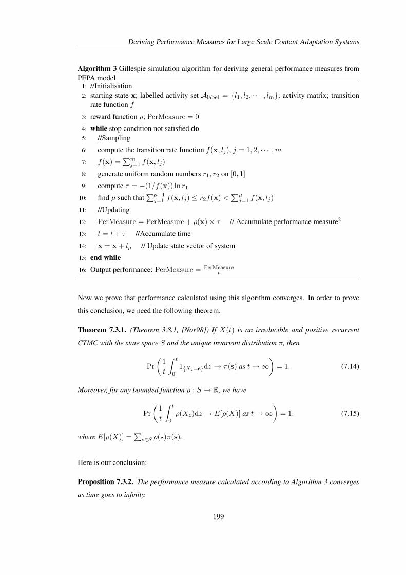
Deriving Performance Measures for Large Scale Content Adaptation Systems
Algorithm 3 Gillespie simulation algorithm for deriving general performance measures fromPEPA model
1: //Initialisation2: starting state x; labelled activity set Alabel = {l1, l2, · · · , lm}; activity matrix; transition
rate function f
3: reward function ρ; PerMeasure = 0
4: while stop condition not satisfied do5: //Sampling
6: compute the transition rate function f(x, lj), j = 1, 2, · · · ,m
7: f(x) =∑m
j=1 f(x, lj)
8: generate uniform random numbers r1, r2 on [0, 1]
9: compute τ = −(1/f(x)) ln r1
10: find µ such that∑µ−1
j=1 f(x, lj) ≤ r2f(x) <∑µ
j=1 f(x, lj)
11: //Updating
12: PerMeasure = PerMeasure + ρ(x)× τ // Accumulate performance measure2
13: t = t + τ //Accumulate time
14: x = x + lµ // Update state vector of system
15: end while16: Output performance: PerMeasure = PerMeasure
t
Now we prove that performance calculated using this algorithm converges. In order to prove
this conclusion, we need the following theorem.
Theorem 7.3.1. (Theorem 3.8.1, [Nor98]) If X(t) is an irreducible and positive recurrent
CTMC with the state space S and the unique invariant distribution π, then
Pr(
1t
∫ t
01{Xz=s}dz → π(s) as t →∞
)= 1. (7.14)
Moreover, for any bounded function ρ : S → R, we have
Pr(
1t
∫ t
0ρ(Xz)dz → E[ρ(X)] as t →∞
)= 1. (7.15)
where E[ρ(X)] =∑
s∈S ρ(s)π(s).
Here is our conclusion:
Proposition 7.3.2. The performance measure calculated according to Algorithm 3 converges
as time goes to infinity.
199
Deriving Performance Measures for Large Scale Content Adaptation Systems
Proof. Assume that n− 1 iterations have been finished and the time has accumulated to tn−1.
Suppose the current one is the n-th iteration and τ is the generated time in this iteration. After
the n-th iteration is finished, the accumulated time will be updated to tn = tn−1 + τ . During
the τ time interval, the simulated CTMC stays in the state x, that is, Xz = x, z ∈ [tn−1, tn).
Therefore,
ρ(x)× τ = ρ(x)∫ tn
tn−1
dz =∫ tn
tn−1
ρ(x)dz =∫ tn
tn−1
ρ(Xz)dz.
That is, the performance calculated in this n-th iteration is∫ tn
tn−1
ρ(Xz)dz. Thus, the perfor-
mance “PerMeasure” accumulated in the previous n− 1 iterations is∫ t1
t0
ρ(Xz)dz +∫ t2
t1
ρ(Xz)dz + · · ·+∫ tn−1
tn−2
ρ(Xz)dz =∫ tn−1
0ρ(Xz)dz.
After updating in this n-th iteration, the performance PerMeasure will be accumulated to∫ tn−1
0ρ(Xz)dz +
∫ tn
tn−1
ρ(Xz)dz =∫ tn
0ρ(Xz)dz.
Therefore,PerMeasure
tn=
1tn
∫ tn
0ρ(Xz)dz.
According to Theorem 7.3.1,1tn
∫ tn
0ρ(Xz)dz → E[ρ(X)] as tn tends to infinity. So the
performance obtained through Algorithm 3 converges as the simulation time goes to infinity.
Performance measure Reward function Alternative wayaveraged population s∗ ρ(s) = s
total variation of s∗ ρ(s) = (s− x∗)T (s− s∗)utilisation of CA4 ρ(s) = s[CA4]
NCA0
s∗[CA4]NCA0
throughput of ca adaptation ρ(s) = s[CA4]rca adaptation s∗[CA4]rca adaptation
response times∗(PDE2) + s∗(PDE3)
s∗(PDE1)× rpde ext cont req
Table 7.2: Deriving performance measures through stochastic simulation
Performance metrics, such as throughput of an activity and utilisation of a local derivative, can
be derived through this algorithm by choosing appropriate reward functions. For example, for
the content adaptation model, some computational methods for common performance measures
have been given in Table 7.2. Particularly in this table, the metric of the total variation of the
200
Deriving Performance Measures for Large Scale Content Adaptation Systems
averaged population cannot be obtained through the fluid approximation approach. When using
Algorithm 3 to derive the throughput of a labelled activity α, we have another choice: the line
12 and line 16 of this algorithm can be respectively replaced by
Thr(α) = Thr(α) + 1{lµ=α},
Thr(α) =Thr(α)
t.
These two new lines account the number of occurrences of α in the total t time. This method is
equivalent to the way of calculating throughput which is presented in Table 7.2.
7.3.4 Comparison of performance measures through different approaches
Until now we have discussed three approaches to deriving performance measures from a PEPA
model. The first way that has been presented in Chapter 2 is to utilise the steady-state probabil-
ity distribution of the CTMC, which can be obtained by solving a matrix equation associated
with the corresponding infinitesimal generator. As we have pointed out, it is not feasible to get
the steady-state distribution when the state space become very large. The other two approaches
are the fluid approximation and stochastic simulation based on our numerical representation
scheme, which have been discussed in the previous subsections. In this subsection, we will
present a comparison between these approaches, in terms of both accuracy and computational
cost, to derive the average response time for the content adaptation system.
7.3.4.1 Comparison in small scale case
According to Little’s law and as the formula (7.12) shows, the average response time can be cal-
culated based on the averaged populations of PDE1, PDE2, PDE3. We have three different
approaches to obtain these populations. The first way, named “solving generator” for conve-
nience, is to get the expected populations based on the steady-state probability distribution,
which is obtained by solving the global balance equation relating to the infinitesimal generator.
This process can be automatically carried out by the PEPA Eclipse plug-in.
The second method is to numerically solve the corresponding ODEs (using the Euler difference
algorithm) to derive the equilibrium, from which the populations of PDEi (i = 1, 2, 3) are
available. The last approach is to employ Algorithm 3 to simulate the CTMC and get the
201
Deriving Performance Measures for Large Scale Content Adaptation Systems
averaged populations. We should point out that Algorithm 3 is designed for simulating the
underlying CTMC in the usual sense, which is also the first CTMC in the density-dependent
family CTMCs underlying the same model, i.e. the CTMC X1(t) with the concentration level
one. When the algorithm is utilised to simulate the CTMC Xn(t) of concentration level n,
according to the definition of density dependent in Chapter 5, it should be modified as follows:
in the algorithm each transition vector lj must be replaced by lj/n and each transition rate
function f(x, lj) be replaced by f(x, lj/n).
Suppose there is one AM, one CA and one C/S Provider in the content adaptation system, i.e.
(N,P, Q) = (1, 1, 1). The number of PDEs varies from one to ten. The experimental results
obtained through the three approaches are presented in Figure 7.5 (a). Of course, the approach
of “solving generator” provides the exact performance of the CTMC, i.e. the CTMC with the
concentration level one, see the red curve. The simulated results with the concentration level
one is coincident with the red curve, reflecting the consistence between the approach of “solving
generator” and the approach of simulation to derive the performance from the same CTMC. As
the level increases, the simulated performance approximates the blue curve which represents
the results obtained by the fluid approximation approach. This is consistent with the conclusion
that the ODEs are the limit of a family of density-dependent CTMCs as the concentration level
tends to infinity. As Figure 7.5 (a) shows, there is a gap between the red and blue curves,
indicating that for a small scale system the performance derived using fluid approximation may
differ from the exact performance of the system. This difference results from the fact that the
fluid approximation only captures the information about the CTMC with concentration level
infinity rather than with level one. However, as we will see later, as the system scale increases,
this difference will decrease to an acceptable level.
We would like to use relative errors to measure this kind of difference. The relative error of
a result obtained by a method is defined as the relative difference between this result and the
result derived by the simulation with the concentration level one, that is
relative error =| result by the other method− result by SSA with concentration level one) |
result by SSA with concentration level one.
In the case of small scale modelling, the reference for calculating relative error should be re-
placed by the numerical solution of the CTMC, as long as it is available. The information of the
relative error about the results presented in Figure 7.5 (a) is given in Figure 7.5 (b). The relative
errors between the exact performance and those obtained through the fluid approximation way
202
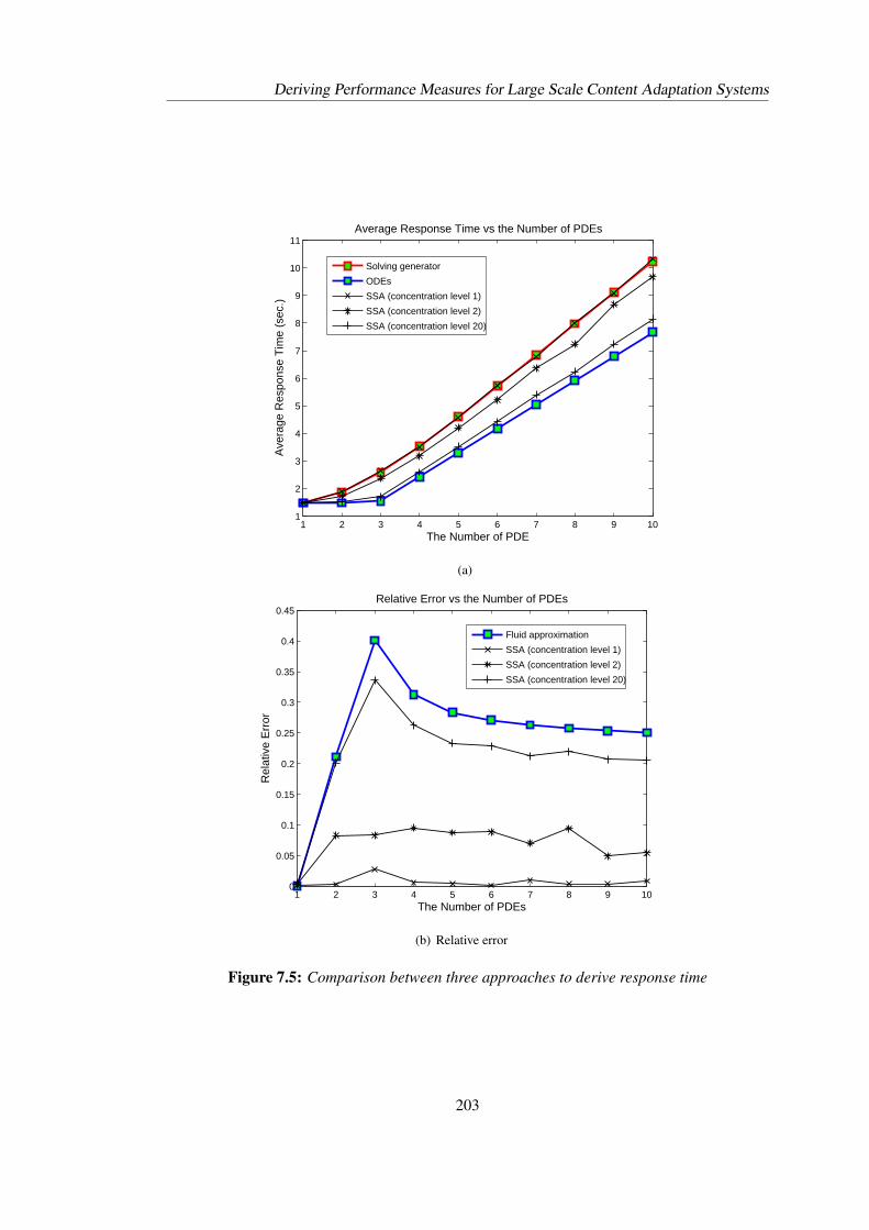
Deriving Performance Measures for Large Scale Content Adaptation Systems
1 2 3 4 5 6 7 8 9 101
2
3
4
5
6
7
8
9
10
11
The Number of PDE
Ave
rage
Res
pons
e T
ime
(sec
.)
Average Response Time vs the Number of PDEs
Solving generator
ODEs
SSA (concentration level 1)
SSA (concentration level 2)
SSA (concentration level 20)
(a)
1 2 3 4 5 6 7 8 9 100
0.05
0.1
0.15
0.2
0.25
0.3
0.35
0.4
0.45
The Number of PDEs
Rel
ativ
e E
rror
Relative Error vs the Number of PDEs
Fluid approximation
SSA (concentration level 1)
SSA (concentration level 2)
SSA (concentration level 20)
(b) Relative error
Figure 7.5: Comparison between three approaches to derive response time
203
Deriving Performance Measures for Large Scale Content Adaptation Systems
are generally greater than 25%, while they reach a peak at the critical point three, which is also
a turning point of the blue curve. As the concentration level decreases, the relative errors of the
simulated results decrease. As we can see, when the concentration level decreases from twenty
to two, the relative errors decrease from more than 20% to less than 10%. The relative errors
are almost zero when the concentration level is one.
The computational cost of these experiments, mainly in terms of running times, is presented
in Table 7.3. These experiments, except for those obtained through the “solving generator”
approach, are carried out using Matlab 7.8.0 (R2009a) on a 2.66GHz Xeon CPU with 4Gb
RAM runing Scientific Linux 5. As seen from Figure 7.1-7.4 in Section 7.2.2, the solutions of
the ODEs will achieve the equilibria before time 20, so the stop time for the fluid approximation
is set as T = 20. The stop time for the simulation using Algorithm 3 is set as T = 5000,
since it can finally make the relative errors of the accumulated performance in two consecutive
iterations less than 5%.
Solving ODEs: SSA: SSA SSA(M,N,P, Q) generator T = 20 T = 5000 T = 5000 T = 5000
step length 10−5 n = 1 n = 2 n = 20(i, 1, 1, 1) < 1.3 1.5885 3.0512 10.2321 378.4077
i = 1, · · · , 10
Table 7.3: Running times (sec.) of small scale experiments
There is no doubt that for small scale modelling in which the steady probability distribution can
be obtained, the approach “solving generator” is promising, because it gives exact performance
values at a low running time. The simulation approach can also provide a similar accuracy, but
the computational cost is higher. The cost of the approach of fluid approximation is low but the
accuracy is also low.
7.3.4.2 Comparison in large scale case
When there are 20 AMs, 20 CAs, 20 C/S Providers in the system, calculating the steady-state
probability distribution by the PEPA Eclipse plug-in becomes infeasible. We have to rely on
the approaches of fluid approximation and stochastic simulation to get performance measures.
As we can see from Figure 7.6 (a) and (b), the fluid approximation can achieve good accuracy.
The relative errors of the results obtained using the fluid approximation are about 6%. Here the
reference for calculating relative errors is the simulated results with the concentration level one,
204
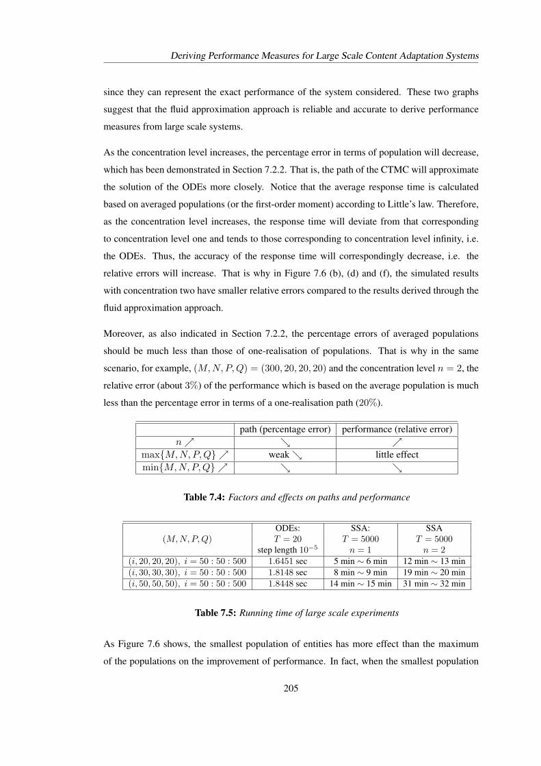
Deriving Performance Measures for Large Scale Content Adaptation Systems
since they can represent the exact performance of the system considered. These two graphs
suggest that the fluid approximation approach is reliable and accurate to derive performance
measures from large scale systems.
As the concentration level increases, the percentage error in terms of population will decrease,
which has been demonstrated in Section 7.2.2. That is, the path of the CTMC will approximate
the solution of the ODEs more closely. Notice that the average response time is calculated
based on averaged populations (or the first-order moment) according to Little’s law. Therefore,
as the concentration level increases, the response time will deviate from that corresponding
to concentration level one and tends to those corresponding to concentration level infinity, i.e.
the ODEs. Thus, the accuracy of the response time will correspondingly decrease, i.e. the
relative errors will increase. That is why in Figure 7.6 (b), (d) and (f), the simulated results
with concentration two have smaller relative errors compared to the results derived through the
fluid approximation approach.
Moreover, as also indicated in Section 7.2.2, the percentage errors of averaged populations
should be much less than those of one-realisation of populations. That is why in the same
scenario, for example, (M,N,P, Q) = (300, 20, 20, 20) and the concentration level n = 2, the
relative error (about 3%) of the performance which is based on the average population is much
less than the percentage error in terms of a one-realisation path (20%).
path (percentage error) performance (relative error)n↗ ↘ ↗
max{M,N,P, Q} ↗ weak ↘ little effectmin{M,N,P, Q} ↗ ↘ ↘
Table 7.4: Factors and effects on paths and performance
ODEs: SSA: SSA(M,N,P, Q) T = 20 T = 5000 T = 5000
step length 10−5 n = 1 n = 2(i, 20, 20, 20), i = 50 : 50 : 500 1.6451 sec 5 min ∼ 6 min 12 min ∼ 13 min(i, 30, 30, 30), i = 50 : 50 : 500 1.8148 sec 8 min ∼ 9 min 19 min ∼ 20 min(i, 50, 50, 50), i = 50 : 50 : 500 1.8448 sec 14 min ∼ 15 min 31 min ∼ 32 min
Table 7.5: Running time of large scale experiments
As Figure 7.6 shows, the smallest population of entities has more effect than the maximum
of the populations on the improvement of performance. In fact, when the smallest population
205
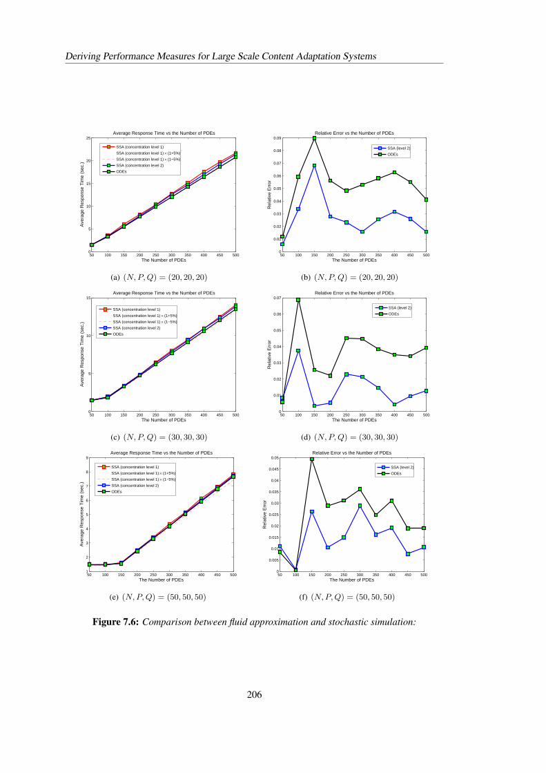
Deriving Performance Measures for Large Scale Content Adaptation Systems
50 100 150 200 250 300 350 400 450 5000
5
10
15
20
25
The Number of PDEs
Ave
rage
Res
pons
e T
ime
(sec
.)
Average Response Time vs the Number of PDEs
SSA (concentration level 1)
SSA (concentration level 1) × (1+5%)
SSA (concentration level 1) × (1−5%)
SSA (concentration level 2)
ODEs
(a) (N, P, Q) = (20, 20, 20)
50 100 150 200 250 300 350 400 450 5000
0.01
0.02
0.03
0.04
0.05
0.06
0.07
0.08
0.09
The Number of PDEs
Rel
ativ
e E
rror
Relative Error vs the Number of PDEs
SSA (level 2)
ODEs
(b) (N, P, Q) = (20, 20, 20)
50 100 150 200 250 300 350 400 450 5000
5
10
15
The Number of PDEs
Ave
rage
Res
pons
e T
ime
(sec
.)
Average Response Time vs the Number of PDEs
SSA (concentration level 1)
SSA (concentration level 1) × (1+5%)
SSA (concentration level 1) × (1−5%)
SSA (concentration level 2)
ODEs
(c) (N, P, Q) = (30, 30, 30)
50 100 150 200 250 300 350 400 450 5000
0.01
0.02
0.03
0.04
0.05
0.06
0.07
The Number of PDEs
Rel
ativ
e E
rror
Relative Error vs the Number of PDEs
SSA (level 2)
ODEs
(d) (N, P, Q) = (30, 30, 30)
50 100 150 200 250 300 350 400 450 5001
2
3
4
5
6
7
8
9
The Number of PDEs
Ave
rage
Res
pons
e T
ime
(sec
.)
Average Response Time vs the Number of PDEs
SSA (concentration level 1)
SSA (concentration level 1) × (1+5%)
SSA (concentration level 1) × (1−5%)
SSA (concentration level 2)
ODEs
(e) (N, P, Q) = (50, 50, 50)
50 100 150 200 250 300 350 400 450 5000
0.005
0.01
0.015
0.02
0.025
0.03
0.035
0.04
0.045
0.05
The Number of PDEs
Rel
ativ
e E
rror
Relative Error vs the Number of PDEs
SSA (level 2)
ODEs
(f) (N, P, Q) = (50, 50, 50)
Figure 7.6: Comparison between fluid approximation and stochastic simulation:
206
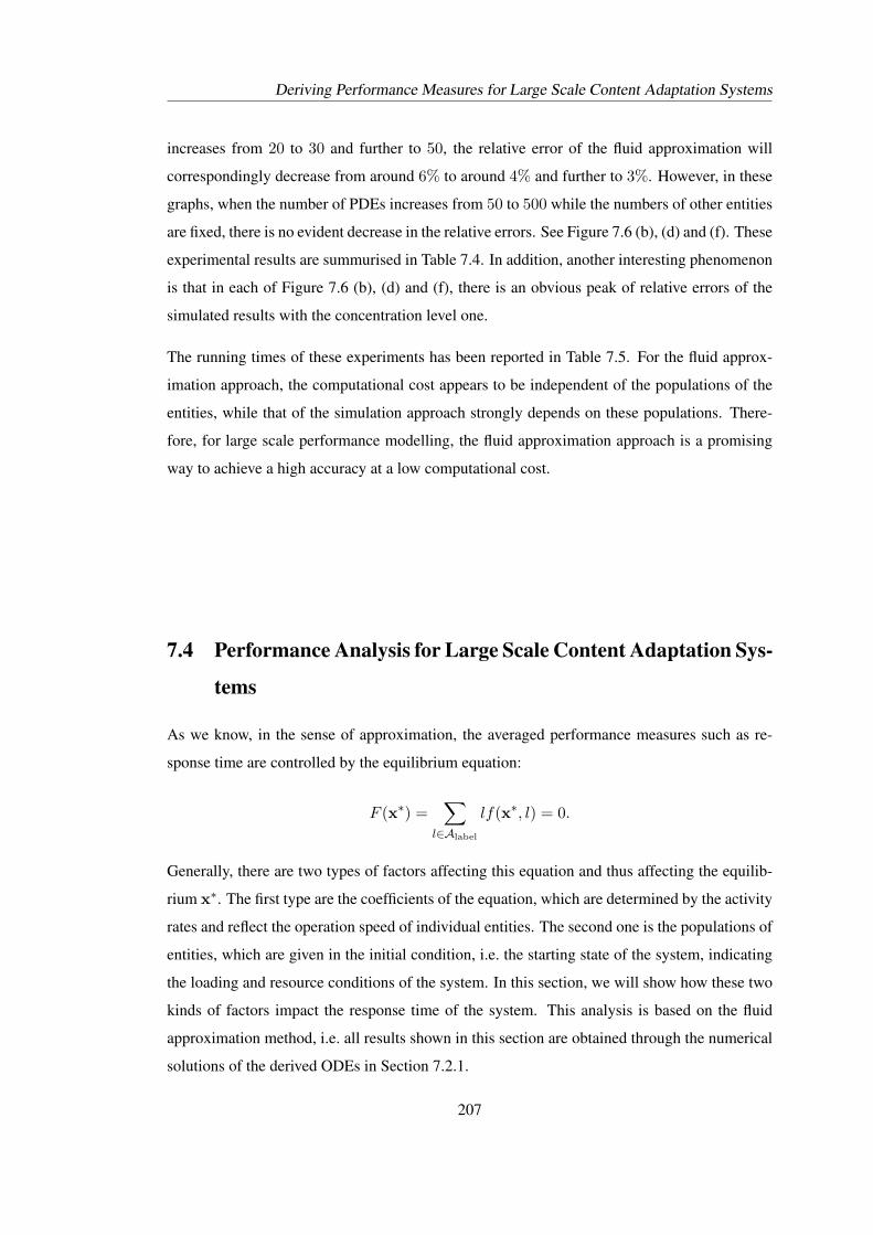
Deriving Performance Measures for Large Scale Content Adaptation Systems
increases from 20 to 30 and further to 50, the relative error of the fluid approximation will
correspondingly decrease from around 6% to around 4% and further to 3%. However, in these
graphs, when the number of PDEs increases from 50 to 500 while the numbers of other entities
are fixed, there is no evident decrease in the relative errors. See Figure 7.6 (b), (d) and (f). These
experimental results are summurised in Table 7.4. In addition, another interesting phenomenon
is that in each of Figure 7.6 (b), (d) and (f), there is an obvious peak of relative errors of the
simulated results with the concentration level one.
The running times of these experiments has been reported in Table 7.5. For the fluid approx-
imation approach, the computational cost appears to be independent of the populations of the
entities, while that of the simulation approach strongly depends on these populations. There-
fore, for large scale performance modelling, the fluid approximation approach is a promising
way to achieve a high accuracy at a low computational cost.
7.4 Performance Analysis for Large Scale Content Adaptation Sys-
tems
As we know, in the sense of approximation, the averaged performance measures such as re-
sponse time are controlled by the equilibrium equation:
F (x∗) =∑
l∈Alabel
lf(x∗, l) = 0.
Generally, there are two types of factors affecting this equation and thus affecting the equilib-
rium x∗. The first type are the coefficients of the equation, which are determined by the activity
rates and reflect the operation speed of individual entities. The second one is the populations of
entities, which are given in the initial condition, i.e. the starting state of the system, indicating
the loading and resource conditions of the system. In this section, we will show how these two
kinds of factors impact the response time of the system. This analysis is based on the fluid
approximation method, i.e. all results shown in this section are obtained through the numerical
solutions of the derived ODEs in Section 7.2.1.
207
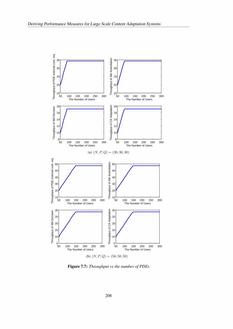
Deriving Performance Measures for Large Scale Content Adaptation Systems
50 100 150 200 250 30015
20
25
30
35
The Number of UsersThr
ough
put o
f PD
E e
xter
nal c
ont.
req.
50 100 150 200 250 30015
20
25
30
35
The Number of Users
Thr
ough
put o
f AM
Ass
imila
tion
50 100 150 200 250 3008
10
12
14
16
18
The Number of Users
Thr
ough
put o
f AM
Dec
isio
n
50 100 150 200 250 3008
10
12
14
16
18
The Number of Users
Thr
ough
put o
f CA
Ada
ptat
ion
(a) (N, P, Q) = (30, 30, 30)
50 100 150 200 250 30010
20
30
40
50
60
The Number of UsersThr
ough
put o
f PD
E e
xter
nal c
ont.
req.
50 100 150 200 250 30010
20
30
40
50
60
The Number of Users
Thr
ough
put o
f AM
Ass
imila
tion
50 100 150 200 250 3005
10
15
20
25
30
The Number of Users
Thr
ough
put o
f AM
Dec
isio
n
50 100 150 200 250 3005
10
15
20
25
30
The Number of Users
Thr
ough
put o
f CA
Ada
ptat
ion
(b) (N, P, Q) = (50, 50, 50)
Figure 7.7: Throughput vs the number of PDEs
208
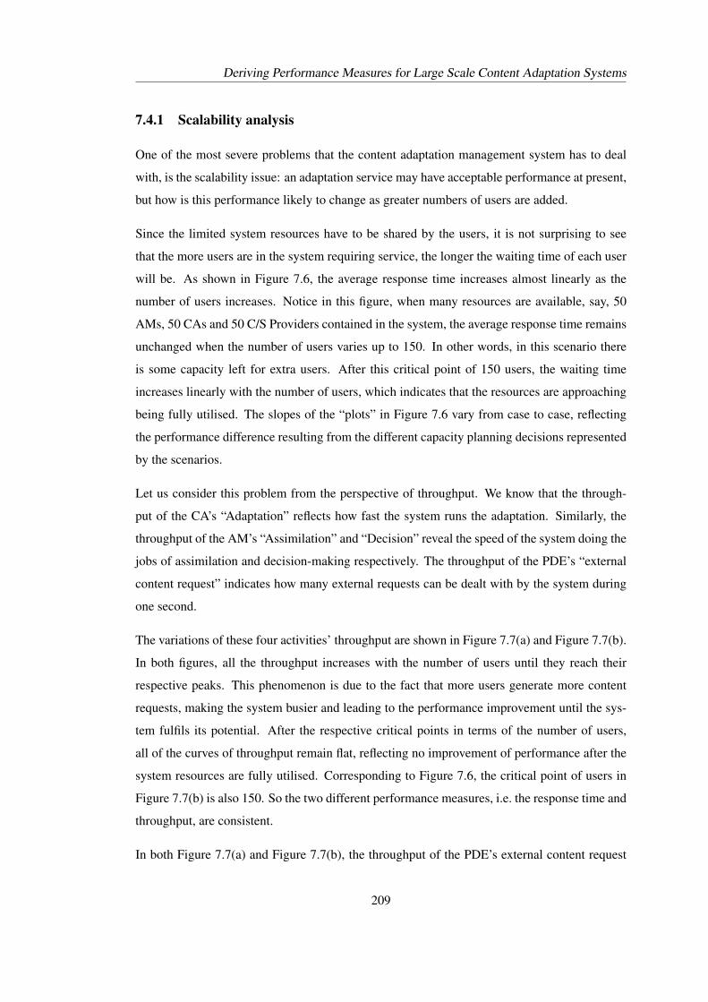
Deriving Performance Measures for Large Scale Content Adaptation Systems
7.4.1 Scalability analysis
One of the most severe problems that the content adaptation management system has to deal
with, is the scalability issue: an adaptation service may have acceptable performance at present,
but how is this performance likely to change as greater numbers of users are added.
Since the limited system resources have to be shared by the users, it is not surprising to see
that the more users are in the system requiring service, the longer the waiting time of each user
will be. As shown in Figure 7.6, the average response time increases almost linearly as the
number of users increases. Notice in this figure, when many resources are available, say, 50
AMs, 50 CAs and 50 C/S Providers contained in the system, the average response time remains
unchanged when the number of users varies up to 150. In other words, in this scenario there
is some capacity left for extra users. After this critical point of 150 users, the waiting time
increases linearly with the number of users, which indicates that the resources are approaching
being fully utilised. The slopes of the “plots” in Figure 7.6 vary from case to case, reflecting
the performance difference resulting from the different capacity planning decisions represented
by the scenarios.
Let us consider this problem from the perspective of throughput. We know that the through-
put of the CA’s “Adaptation” reflects how fast the system runs the adaptation. Similarly, the
throughput of the AM’s “Assimilation” and “Decision” reveal the speed of the system doing the
jobs of assimilation and decision-making respectively. The throughput of the PDE’s “external
content request” indicates how many external requests can be dealt with by the system during
one second.
The variations of these four activities’ throughput are shown in Figure 7.7(a) and Figure 7.7(b).
In both figures, all the throughput increases with the number of users until they reach their
respective peaks. This phenomenon is due to the fact that more users generate more content
requests, making the system busier and leading to the performance improvement until the sys-
tem fulfils its potential. After the respective critical points in terms of the number of users,
all of the curves of throughput remain flat, reflecting no improvement of performance after the
system resources are fully utilised. Corresponding to Figure 7.6, the critical point of users in
Figure 7.7(b) is also 150. So the two different performance measures, i.e. the response time and
throughput, are consistent.
In both Figure 7.7(a) and Figure 7.7(b), the throughput of the PDE’s external content request
209
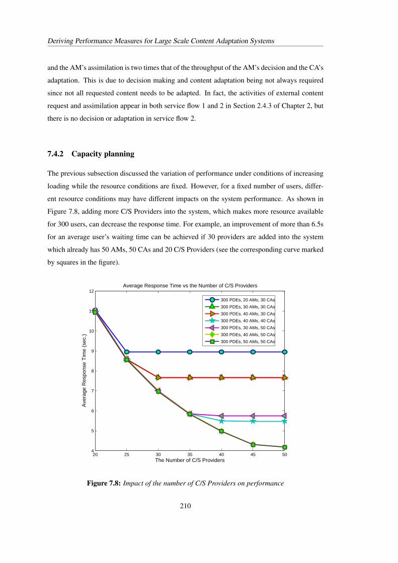
Deriving Performance Measures for Large Scale Content Adaptation Systems
and the AM’s assimilation is two times that of the throughput of the AM’s decision and the CA’s
adaptation. This is due to decision making and content adaptation being not always required
since not all requested content needs to be adapted. In fact, the activities of external content
request and assimilation appear in both service flow 1 and 2 in Section 2.4.3 of Chapter 2, but
there is no decision or adaptation in service flow 2.
7.4.2 Capacity planning
The previous subsection discussed the variation of performance under conditions of increasing
loading while the resource conditions are fixed. However, for a fixed number of users, differ-
ent resource conditions may have different impacts on the system performance. As shown in
Figure 7.8, adding more C/S Providers into the system, which makes more resource available
for 300 users, can decrease the response time. For example, an improvement of more than 6.5s
for an average user’s waiting time can be achieved if 30 providers are added into the system
which already has 50 AMs, 50 CAs and 20 C/S Providers (see the corresponding curve marked
by squares in the figure).
20 25 30 35 40 45 504
5
6
7
8
9
10
11
12
The Number of C/S Providers
Ave
rage
Res
pons
e T
ime
(sec
.)
Average Response Time vs the Number of C/S Providers
300 PDEs, 20 AMs, 30 CAs
300 PDEs, 30 AMs, 30 CAs
300 PDEs, 40 AMs, 30 CAs
300 PDEs, 40 AMs, 40 CAs
300 PDEs, 30 AMs, 50 CAs
300 PDEs, 40 AMs, 50 CAs
300 PDEs, 50 AMs, 50 CAs
Figure 7.8: Impact of the number of C/S Providers on performance
210
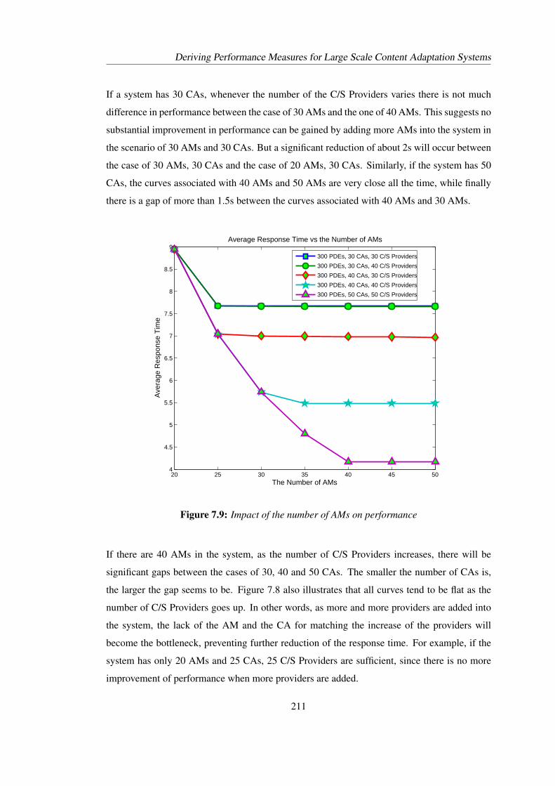
Deriving Performance Measures for Large Scale Content Adaptation Systems
If a system has 30 CAs, whenever the number of the C/S Providers varies there is not much
difference in performance between the case of 30 AMs and the one of 40 AMs. This suggests no
substantial improvement in performance can be gained by adding more AMs into the system in
the scenario of 30 AMs and 30 CAs. But a significant reduction of about 2s will occur between
the case of 30 AMs, 30 CAs and the case of 20 AMs, 30 CAs. Similarly, if the system has 50
CAs, the curves associated with 40 AMs and 50 AMs are very close all the time, while finally
there is a gap of more than 1.5s between the curves associated with 40 AMs and 30 AMs.
20 25 30 35 40 45 504
4.5
5
5.5
6
6.5
7
7.5
8
8.5
9
The Number of AMs
Ave
rage
Res
pons
e T
ime
Average Response Time vs the Number of AMs
300 PDEs, 30 CAs, 30 C/S Providers
300 PDEs, 30 CAs, 40 C/S Providers
300 PDEs, 40 CAs, 30 C/S Providers
300 PDEs, 40 CAs, 40 C/S Providers
300 PDEs, 50 CAs, 50 C/S Providers
Figure 7.9: Impact of the number of AMs on performance
If there are 40 AMs in the system, as the number of C/S Providers increases, there will be
significant gaps between the cases of 30, 40 and 50 CAs. The smaller the number of CAs is,
the larger the gap seems to be. Figure 7.8 also illustrates that all curves tend to be flat as the
number of C/S Providers goes up. In other words, as more and more providers are added into
the system, the lack of the AM and the CA for matching the increase of the providers will
become the bottleneck, preventing further reduction of the response time. For example, if the
system has only 20 AMs and 25 CAs, 25 C/S Providers are sufficient, since there is no more
improvement of performance when more providers are added.
211
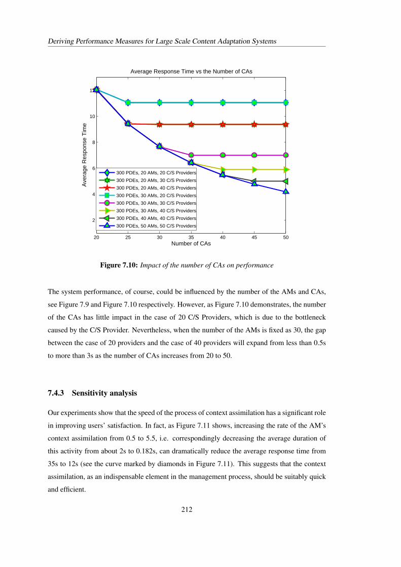
Deriving Performance Measures for Large Scale Content Adaptation Systems
20 25 30 35 40 45 50
2
4
6
8
10
12
Number of CAs
Ave
rage
Res
pons
e T
ime
Average Response Time vs the Number of CAs
300 PDEs, 20 AMs, 20 C/S Providers
300 PDEs, 20 AMs, 30 C/S Providers
300 PDEs, 20 AMs, 40 C/S Providers
300 PDEs, 30 AMs, 20 C/S Providers
300 PDEs, 30 AMs, 30 C/S Providers
300 PDEs, 30 AMs, 40 C/S Providers
300 PDEs, 40 AMs, 40 C/S Providers
300 PDEs, 50 AMs, 50 C/S Providers
Figure 7.10: Impact of the number of CAs on performance
The system performance, of course, could be influenced by the number of the AMs and CAs,
see Figure 7.9 and Figure 7.10 respectively. However, as Figure 7.10 demonstrates, the number
of the CAs has little impact in the case of 20 C/S Providers, which is due to the bottleneck
caused by the C/S Provider. Nevertheless, when the number of the AMs is fixed as 30, the gap
between the case of 20 providers and the case of 40 providers will expand from less than 0.5s
to more than 3s as the number of CAs increases from 20 to 50.
7.4.3 Sensitivity analysis
Our experiments show that the speed of the process of context assimilation has a significant role
in improving users’ satisfaction. In fact, as Figure 7.11 shows, increasing the rate of the AM’s
context assimilation from 0.5 to 5.5, i.e. correspondingly decreasing the average duration of
this activity from about 2s to 0.182s, can dramatically reduce the average response time from
35s to 12s (see the curve marked by diamonds in Figure 7.11). This suggests that the context
assimilation, as an indispensable element in the management process, should be suitably quick
and efficient.
212
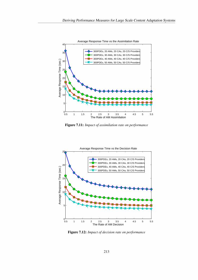
Deriving Performance Measures for Large Scale Content Adaptation Systems
0.5 1 1.5 2 2.5 3 3.5 4 4.5 5 5.50
5
10
15
20
25
30
35
40
The Rate of AM Assimilation
Ave
rage
Res
pons
e T
ime
(sec
.)
Average Response Time vs the Assimilation Rate
300PDEs, 20 AMs, 20 CAs, 20 C/S Providers
300PDEs, 30 AMs, 30 CAs, 30 C/S Providers
300PDEs, 40 AMs, 40 CAs, 40 C/S Providers
300PDEs, 50 AMs, 50 CAs, 50 C/S Providers
Figure 7.11: Impact of assimilation rate on performance
0.5 1 1.5 2 2.5 3 3.5 4 4.5 5 5.50
5
10
15
20
25
The Rate of AM Decision
Ave
rage
Res
pons
e T
ime
(sec
.)
Average Response Time vs the Decision Rate
300PDEs, 20 AMs, 20 CAs, 20 C/S Providers
300PDEs, 30 AMs, 30 CAs, 30 C/S Providers
300PDEs, 40 AMs, 40 CAs, 40 C/S Providers
300PDEs, 50 AMs, 50 CAs, 50 C/S Providers
Figure 7.12: Impact of decision rate on performance
213
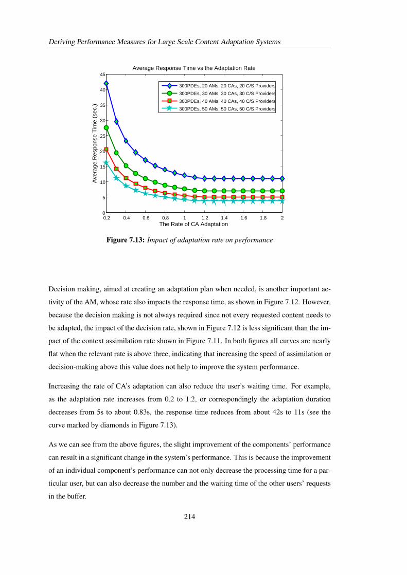
Deriving Performance Measures for Large Scale Content Adaptation Systems
0.2 0.4 0.6 0.8 1 1.2 1.4 1.6 1.8 20
5
10
15
20
25
30
35
40
45
The Rate of CA Adaptation
Ave
rage
Res
pons
e T
ime
(sec
.)
Average Response Time vs the Adaptation Rate
300PDEs, 20 AMs, 20 CAs, 20 C/S Providers
300PDEs, 30 AMs, 30 CAs, 30 C/S Providers
300PDEs, 40 AMs, 40 CAs, 40 C/S Providers
300PDEs, 50 AMs, 50 CAs, 50 C/S Providers
Figure 7.13: Impact of adaptation rate on performance
Decision making, aimed at creating an adaptation plan when needed, is another important ac-
tivity of the AM, whose rate also impacts the response time, as shown in Figure 7.12. However,
because the decision making is not always required since not every requested content needs to
be adapted, the impact of the decision rate, shown in Figure 7.12 is less significant than the im-
pact of the context assimilation rate shown in Figure 7.11. In both figures all curves are nearly
flat when the relevant rate is above three, indicating that increasing the speed of assimilation or
decision-making above this value does not help to improve the system performance.
Increasing the rate of CA’s adaptation can also reduce the user’s waiting time. For example,
as the adaptation rate increases from 0.2 to 1.2, or correspondingly the adaptation duration
decreases from 5s to about 0.83s, the response time reduces from about 42s to 11s (see the
curve marked by diamonds in Figure 7.13).
As we can see from the above figures, the slight improvement of the components’ performance
can result in a significant change in the system’s performance. This is because the improvement
of an individual component’s performance can not only decrease the processing time for a par-
ticular user, but can also decrease the number and the waiting time of the other users’ requests
in the buffer.
214
Deriving Performance Measures for Large Scale Content Adaptation Systems
7.5 Structural Analysis of A Subsystem
In reality, content adaptation management may be rather complex, particularly in a highly
loaded condition, due to the heterogeneity of devices and the diversity of requirements. The
previous section has presented two ways to enhance the system performance: in addition to
improving the performance of individual entities, the system manager could have an alterna-
tive way—capacity planning—to meet the users’ requirements. In both ways, it is important to
know information about the system such as the working states of those entities, for the purpose
of efficiently controlling and optimising the management of the whole. Therefore, in this sec-
tion we will deduce some functional properties of content adaptation systems by the techniques
developed for PEPA that were presented in Chapter 4.
7.5.1 Adaptation management model
For convenience, the illustration of our technique is based on a subsystem of the content adapta-
tion framework, which only consists of the three entities: the AM, the CA and the C/S Provider.
This subsystem can be considered as an external environment to the users, which only conducts
adaptation processes without communication with the users. See Figure 7.14, which illustrates
the working cycle of the subsystem. We should point out that the users as well as the inter-
actions with the users are not considered in this working mechanism. This allows us to place
more emphasis on the management process and pay more attention to the interactions between
the entities which can carry out the management and provide services. Another reason is that,
a realistic system may differ significantly from the system considered in this chapter. A useful
technique which can generally apply is thus more important than a result concluded from a
specific model. Therefore, we emphasise our technique and just use the subsystem to illustrate
the technique in this section.
The PEPA model of the operation of this subsystem can be similarly defined. See below.
215
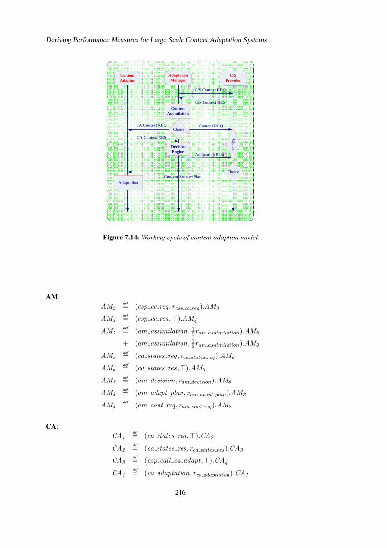
Deriving Performance Measures for Large Scale Content Adaptation Systems
Context Assimilation
Content REQ
Content Source+Plan
Decision Engine
C/S Context REQ
Adaptation
C/SProvider
Content Adaptor
AdaptationManager
C/S Context RES
Choice
Choice
CA Context REQ
CA Context RES
Adaptation PlanC
hoice
Figure 7.14: Working cycle of content adaption model
AM:AM2
def= (csp cc req , rcsp cc req).AM3
AM3def= (csp cc res,>).AM4
AM4def= (am assimilation, 1
2ram assimilation).AM5
+ (am assimilation, 12ram assimilation).AM9
AM5def= (ca states req , rca states req).AM6
AM6def= (ca states res,>).AM7
AM7def= (am decision, ram decision).AM8
AM8def= (am adapt plan, ram adapt plan).AM2
AM9def= (am cont req , ram cont req).AM2
CA:CA1
def= (ca states req ,>).CA2
CA2def= (ca states res, rca states res).CA3
CA3def= (csp call ca adapt ,>).CA4
CA4def= (ca adaptation, rca adaptation).CA1
216
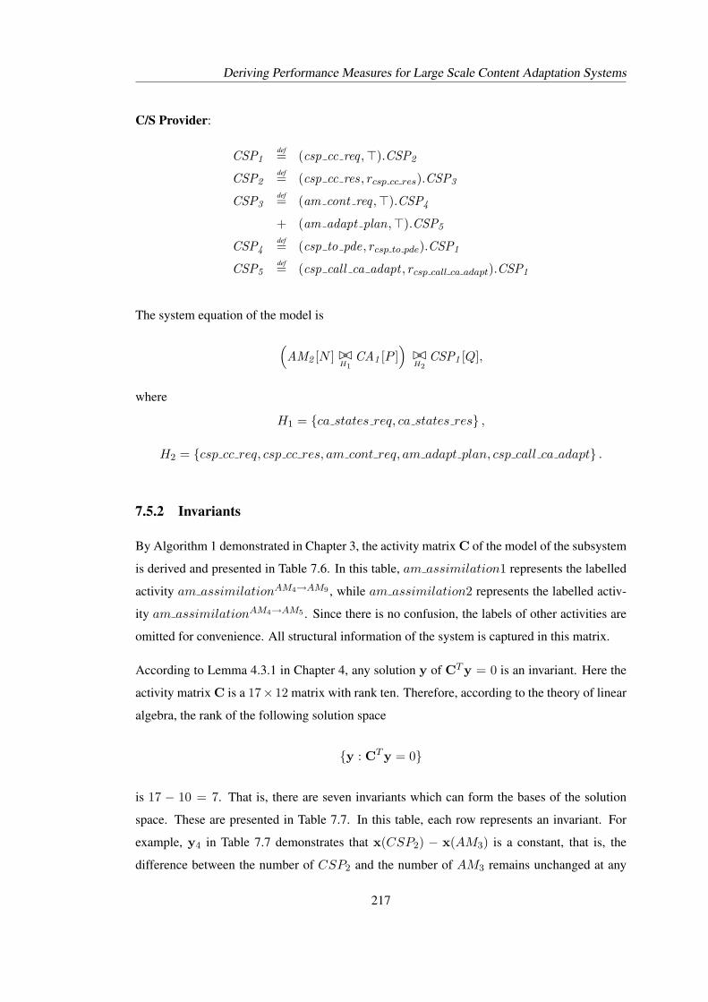
Deriving Performance Measures for Large Scale Content Adaptation Systems
C/S Provider:
CSP1def= (csp cc req ,>).CSP2
CSP2def= (csp cc res, rcsp cc res).CSP3
CSP3def= (am cont req ,>).CSP4
+ (am adapt plan,>).CSP5
CSP4def= (csp to pde, rcsp to pde).CSP1
CSP5def= (csp call ca adapt , rcsp call ca adapt).CSP1
The system equation of the model is
(AM2 [N ] BC
H1CA1 [P ]
)BCH2
CSP1 [Q],
where
H1 = {ca states req, ca states res} ,
H2 = {csp cc req, csp cc res, am cont req, am adapt plan, csp call ca adapt} .
7.5.2 Invariants
By Algorithm 1 demonstrated in Chapter 3, the activity matrix C of the model of the subsystem
is derived and presented in Table 7.6. In this table, am assimilation1 represents the labelled
activity am assimilationAM4→AM9 , while am assimilation2 represents the labelled activ-
ity am assimilationAM4→AM5 . Since there is no confusion, the labels of other activities are
omitted for convenience. All structural information of the system is captured in this matrix.
According to Lemma 4.3.1 in Chapter 4, any solution y of CTy = 0 is an invariant. Here the
activity matrix C is a 17× 12 matrix with rank ten. Therefore, according to the theory of linear
algebra, the rank of the following solution space
{y : CTy = 0}
is 17 − 10 = 7. That is, there are seven invariants which can form the bases of the solution
space. These are presented in Table 7.7. In this table, each row represents an invariant. For
example, y4 in Table 7.7 demonstrates that x(CSP2) − x(AM3) is a constant, that is, the
difference between the number of CSP2 and the number of AM3 remains unchanged at any
217
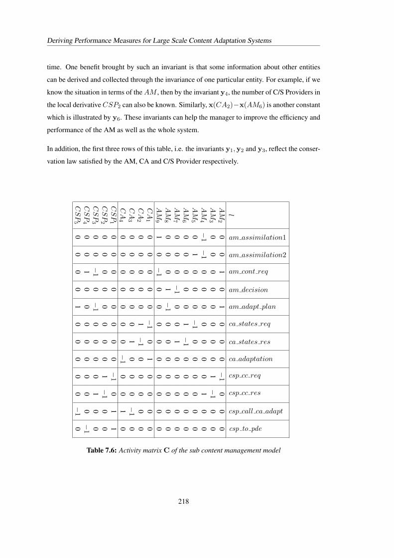
Deriving Performance Measures for Large Scale Content Adaptation Systems
time. One benefit brought by such an invariant is that some information about other entities
can be derived and collected through the invariance of one particular entity. For example, if we
know the situation in terms of the AM , then by the invariant y4, the number of C/S Providers in
the local derivative CSP2 can also be known. Similarly, x(CA2)−x(AM6) is another constant
which is illustrated by y6. These invariants can help the manager to improve the efficiency and
performance of the AM as well as the whole system.
In addition, the first three rows of this table, i.e. the invariants y1,y2 and y3, reflect the conser-
vation law satisfied by the AM, CA and C/S Provider respectively.l
am assimilation1
am assimilation2
am cont req
am decision
am adapt plan
ca states req
ca states res
ca adaptation
csp cc req
csp cc res
csp call ca adapt
csp to pde
AM
20
01
01
00
0−
10
00
AM
30
00
00
00
01
−1
00
AM
4−
1−
10
00
00
00
10
0A
M5
01
00
0−
10
00
00
0A
M6
00
00
01
−1
00
00
0A
M7
00
0−
10
01
00
00
0A
M8
00
01
−1
00
00
00
0A
M9
10
−1
00
00
00
00
0C
A1
00
00
0−
10
10
00
0C
A2
00
00
01
−1
00
00
0C
A3
00
00
00
10
00
−1
0C
A4
00
00
00
0−
10
01
0C
SP
10
00
00
00
0−
10
11
CS
P2
00
00
00
00
1−
10
0C
SP
30
0−
10
−1
00
00
10
0C
SP
40
01
00
00
00
00
−1
CS
P5
00
00
10
00
00
−1
0
Table 7.6: Activity matrix C of the sub content management model
218
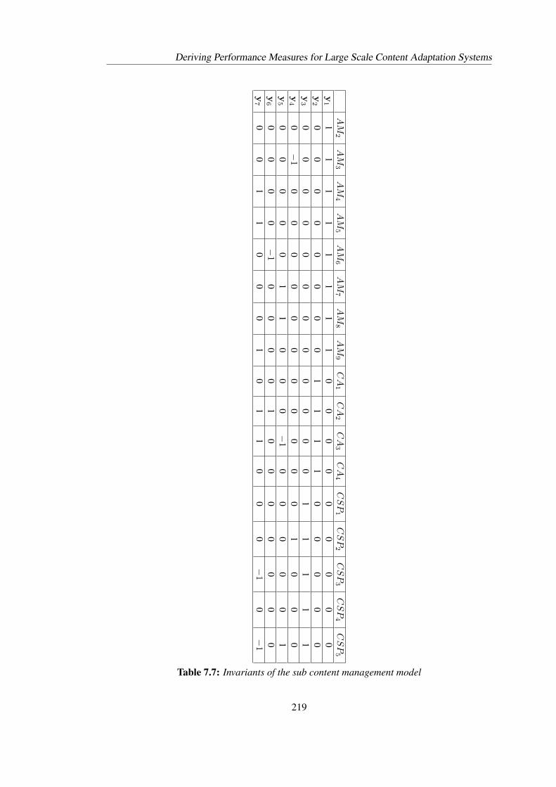
Deriving Performance Measures for Large Scale Content Adaptation Systems
AM
2A
M3
AM
4A
M5
AM
6A
M7
AM
8A
M9
CA
1C
A2
CA
3C
A4
CS
P1
CS
P2
CS
P3
CS
P4
CS
P5
y1
11
11
11
11
00
00
00
00
0y
20
00
00
00
01
11
10
00
00
y3
00
00
00
00
00
00
11
11
1y
40
−1
00
00
00
00
00
01
00
0y
50
00
00
11
00
0−
10
00
00
1y
60
00
0−
10
00
01
00
00
00
0y
70
01
10
00
10
11
00
0−
10
−1
Table 7.7: Invariants of the sub content management model
219
Deriving Performance Measures for Large Scale Content Adaptation Systems
7.5.3 Deadlock-checking
One important issue in protocol design for content adaptation as well as other systems is to
avoid deadlocks, which can make a system become stuck in a particular state. In Chapter 4, we
have provided a structure-based algorithm, i.e. Algorithm 2, to check deadlocks for large scale
systems.
We should point out that the model considered here is not equal conflict. In fact, we know
that from the activity matrix, pre(am cont req) ∩ pre(am adapt plan) = {CSP3} but they
are not equal. So, according to Proposition 4.4.1 in Chapter 4, the model is not equal conflict.
However, as discussed in Section 4.5.3, we can still apply this algorithm to the content adapta-
tion system. That is, if there are no deadlocks in the generalised state space of the system which
is checked by the Algorithm 2, then this system has no deadlocks. Fortunately, according to our
analysis using Algorithm 2, in our model what ever the populations of N,P and Q are, there
are no deadlocks in the linearised state space, so the protocol represented by the working cycle
has no deadlocks.
Of course, we can do more qualitative analysis for content adaptation systems, as long as mature
designs and concrete protocols are available.
7.6 Summary
This chapter has experimentally illustrated some fundamental characteristics of the fluid ap-
proximation of PEPA models, particularly with a focus on the convergence and consistence
properties. In addition, this chapter has demonstrated the kind of performance measures sup-
ported by the fluid approximation approach and how they can be derived. In particular, this
chapter revealed that the average performance is approximately governed by a set of corre-
sponding nonlinear algebra equations, which can help to optimise a system in a simple and
efficient way. For those metrics that cannot be obtained through this approach, we have pro-
posed a numerical representation scheme-based stochastic simulation algorithm, along with a
proof of the convergence of this algorithm. Detailed comparisons and analysis of performance
derivation through different approaches have been presented.
This chapter has shown the performance analysis of the large scale content adaptation system.
The numerical results from the evaluation were presented and analysed to determine the fac-
220

Deriving Performance Measures for Large Scale Content Adaptation Systems
tors that affect the system performance. The analysis of the sensitivity and scalability of the
response time has the potential to have great bearing on the continuing design of the content
adaptation system and the capacity planning of future implementations. Moreover, this chap-
ter has presented some qualitative analysis for a subsystem of content adaptation, in which
invariance analysis as well as deadlock-checking was briefly discussed.
221

222
Chapter 8
Conclusions
8.1 Introduction
In this final chapter the main results of the thesis are summarised. Then several topics for
further research are presented. This will conclude the main body of the thesis.
8.2 Summary
The work presented in this thesis addresses the technical and theoretical development for the
formalism PEPA to overcome the state-space explosion problem and make it suitable to validate
and evaluate large scale computer and communications systems. Our work embodies three
levels of the process of performance modelling: model representation, computational approach
and performance derivation.
As a high-level modelling language, the syntactic nature of PEPA makes the models eas-
ily understood by human beings. However, this advantage becomes a disadvantage for ma-
chines/computers (as well as for human beings) to directly carry out qualitative or quantitative
analysis of PEPA. The numerical representation scheme for PEPA proposed in this thesis will
make this analysis more direct and convenient. In this scheme, the correspondence between ac-
tions in PEPA and transitions in the underlying CTMC has been made to be one-to-one through
the definition of labelled activities. Modified activity matrices have been defined based on
labelled activities to capture the structural information of PEPA models, while transition rate
functions were proposed to capture the timing information. Since all the information of a PEPA
model is described and represented numerically by these definitions, based on them it is easy to
extract and simulate the underlying CTMC and derive the fluid approximation. Moreover, this
new presentation has lead to the finding: there is a P/T structure underlying each PEPA model,
which reveals the strong connection between stochastic process algebras and stochastic Petri
nets.
223
Conclusions
The scheme has been proved consistent with the original semantics of PEPA. An algorithm
for automatically deriving the numerical representation scheme, and thus the underlying P/T
structure and the fluid approximation, from any given PEPA model has been proposed. In addi-
tion, some investigations of the representation scheme were carried out. In particular, we have
proved that using numerical vector forms to represent system states can significantly reduce the
size of the state space of the system, i.e., the exponential increase of the size of the state space
with the number of components can be reduced to at most polynomial increase.
Two important issues regarding structural and fluid-flow analysis were investigated in this the-
sis. These studies which were facilitated by the new representation scheme, have verified the
associated computational approaches with PEPA.
The first issue was to develop approaches and techniques of the qualitative analysis for large
scale PEPA models. Based on the underlying P/T structure and the theories developed for Petri
nets, we have established powerful methods to derive and store the state space for a class of
PEPA models without suffering the state-space explosion problem. Invariants in the context
of PEPA were defined, and the method of how to find them was given. A conservation law
was discussed, which was a particular kind of invariance, stating that the population of each
component type is constant. The other kind of invariance expresses the coupling between dif-
ferent component types, i.e., the cooperations ensure that the numbers of local derivatives in
the synchronised components always change together. Invariants could be used for qualitative
reasoning about systems and to prove the convergence of the solution of the derived ODEs.
As an important part of the structural analysis for PEPA, a new deadlock-checking approach
has been proposed to avoid the state-space explosion problem, which can not only efficiently
carry out checking for a particular system but can tell when and how a system structure leads
to deadlocks.
The second issue was the theoretical development for the fluid approximation of PEPA models.
In this thesis, based on the numerical representation scheme, an improved mapping from PEPA
to ODEs has been proposed, which extended the current mapping semantics of fluid approxi-
mations. The derived ODEs could be considered as the limit of a family of density dependent
CTMCs underlying the given PEPA model. We have established the fundamental characteristics
of the derived ODEs, including the existence, uniqueness, boundedness and nonnegativeness
of the solution. The convergence of the solution as time tends to infinity for general PEPA
models, has been proved under a particular condition. This particular condition relates some
224
Conclusions
famous constants of Markov chains such as the spectral gap and the Log-Sobolev constant. For
a class of PEPA models with two component types and one synchronisation, the convergence
under some mild conditions that can be easily checked, as has been proved through a purely
analytical approach. The coefficient matrices of the derived ODEs were studied: their eigenval-
ues are either zeros or have negative real parts. The structural property of invariance has been
shown to play an important role in the proof of convergence for some PEPA models.
This thesis has established the consistency between the fluid approximation and the underlying
CTMC for PEPA. We have proved that for a PEPA model without synchronisations, the so-
lution of the derived ODEs converges and the limit coincides with the steady-state probability
distribution of the underlying CTMC. For a model with synchronisations, the limit of the so-
lution is consistent with the steady-state probability distribution corresponding to a family of
underlying density dependent CTMCs underlying this model. This consistency has also been
illustrated by the numerical comparisons between the fluid approximation and the simulations
of the CTMCs underlying the content adaptation system.
Another important issue, deriving performance measures from large scale PEPA models, was
also addressed in this thesis. We have shown that only the performance metrics that depend on
the averaged population or that can be represented by a Markov reward function, can be derived
from the fluid approximation of a PEPA model. In order to obtain those measures that cannot
be obtained through this approach, we have provided a stochastic simulation algorithm which
is based on the numerical representation scheme, together with a proof of the convergence of
this algorithm.
These enhancements and investigations of PEPA have been applied to evaluate the large scale
content adaptation systems, where both qualitative and quantitative analysis has been carried
out. The main quantitative performance metric considered was the response time, derived from
the fluid approximation of the model according to Little’s law. Our results particularly showed
that the average response time increased almost linearly as the number of users increased when
the resources were fully utilised. On the other hand, for a fixed number of users, more resource
could help to reduce the response time. But as more and more of a particular type of resource
were added into the system, the lack of the other types of resource to match the increase in this
particular type of resource would become the bottleneck, preventing further reduction of the
response time. This suggested the need for capacity planning and optimisation of content adap-
tation systems. This thesis revealed that the average response time is approximately governed
225
Conclusions
by a set of corresponding nonlinear algebra equations. Based on these equations, sensitivity
and scalability analysis, and capacity planning and optimisation for large scale systems could
be made simpler and more efficient. In addition, some structural analysis of a subsystem of
content adaptation has been presented.
PEPA with these associated techniques and methods is expected to have more applications in
large scale systems in the future. Because there is no mature and complete protocol being
proposed for content adaptation at the current moment, there is no corresponding complete
protocol validation for the content adaptation system. However, we have provided many pow-
erful techniques for the validation and evaluation for the future design of the content adaptation
system. Therefore, not only large scale content adaptation systems but other computer and
communications systems can be validated and evaluated by PEPA.
8.3 Limitations of the thesis and Future work
In this section, we address limitations of our work. Several topics for future research will be
presented, which are motivated by those limitations as well as the achievements presented in
this thesis.
The main limitation of our work is that many results shown in this thesis have certain restric-
tions. For example, the equivalent deadlock-checking theory (Theorem 4.5.5) presented in
Chapter 4 was proved only for a class of EQ systems rather than general systems. The con-
vergence result shown in Chapter 5 was obtained under a particular condition that cannot be
easily verified currently. In Chapter 6, the convergence was demonstrated only for some typ-
ical classes of PEPA models. As a future work, we will investigate whether these restrictions
are necessary and how to weaken or remove them if they are unnecessary. In particular, the
conjecture that the particular condition is satisfied by any PEPA model, i.e. the open problem
given in Chapter 5, should be proved or negated in the future. Since this condition relates the
convergence problem to some famous constants of Markov chains, future investigation of this
aspect can expand our understanding of the CTMCs underlying PEPA models.
In this thesis, the consistency between the ODEs and the CTMCs was demonstrated in an
asymptotic sense, i.e. in the situation of the concentration level tending to infinity. In prac-
tice, as shown by the experiments in Chapter 7, the approximation between the ODEs and the
CTMCs at finite concentration levels, both in terms of population and performance measure, are
226
Conclusions
of interest and thus need to be theoretically measured. Future work should involve theoretical
error estimation for this approximation.
In Chapter 7, we have suggested the appropriate approaches to derive performance measures
for small and large scale modelling respectively. However, we have not considered the middle
scale case. A middle scale PEPA model is one where the numerical solution of the underlying
CTMC is not available while the fluid-approximated result is not accurate. Although stochastic
simulations can be used to derive performance measures for middle scale PEPA models, we
still need to investigate how to derive these measures at a low computational cost for middle
scale modelling.
In the context of probability theory and stochastic processes, the theory of large deviation was
developed to study the asymptotics of probabilities of rare events with the help of variational
problems, see [DZ98, FK06] for an introduction. This theory has been widely used for perfor-
mance analysis [SW95] and been successfully applied to queueing networks [SW95, O’C95,
SG95, AD98]. But to the best of our knowledge, there are no discussions of this theory in the
context of stochastic process algebras. However, this theory could be expected to be helpful in
the quantitative analysis using PEPA. For example, since the simulated performance measures
are obtained or collected within finite time or finite iterations, their deviation from the expected
ones, which can be represented by rare events, should be understood and estimated. Large de-
viation theory is a good method to investigate such deviation. We plan to apply this theory to
the PEPA language in the future.
The future work mentioned above is mainly stimulated by the limitations of the current work.
However, there are some topics for future research, which are motivated by the achievements.
For example, we have established the relationship and connections between PEPA and Petri
nets, which provides a new approach to investigate PEPA as well as Petri nets. Through the re-
vealed connections, not only the work for Petri nets can be established parallel and analogously
in the context of PEPA, but the theories and techniques developed for PEPA can also be applied
to Petri nets. For example, our achievements on the fluid approximation such as the convergence
and consistency results, can be expected to apply to Petri nets. To the best of our knowledge,
although there is plenty of work on fluid approximation of Petri nets (e.g. [SR05,MRS06]), but
there are no results on the problem of the convergence with respect to time, i.e. whether the
solution converges as time tends to infinity. Investigation in this aspect, both in terms of PEPA
and Petri nets, is one area of our future work.
227
Conclusions
As illustrated by the new deadlock-checking method presented in Chapter 4, the structure-based
approach is powerful in the qualitative analysis of PEPA models. Future work is needed to study
some other qualitative problems based on this approach, such as logical model-checking and
qualitative reasoning [BGH09].
When the rates of change within the system model are generalised to allow activity rates to
be governed by probability distributions rather than being deterministic, or more uncertainty
is involved, the evolution of the system can be described by a set of stochastic differential
equations (SDEs) [Hil05a]. Some preliminary study, particularly on the mapping semantics
and some interpretation, has been presented in [Hay07b, Sle09]. But many problems have not
been solved. For example, the positiveness of the solution of the derived SDEs, the relationship
with stochastic simulations, as well as some characteristics (e.g. exponential stability [Mao94]).
These problems lead to a direction for future research for PEPA.
Our research addressed in this thesis was carried out in the context of PEPA. Now the PEPA lan-
guage has been extended into Bio-PEPA to model and analyse biochemical networks [CH09].
For the Bio-PEPA formalism, there are similar problems and issues under investigation, such
as qualitative and quantitative analysis for Bio-PEPA models [Gue09]. Our achievements, such
as the structure-based method for qualitative analysis and the theoretical developments for fluid
approximations, can be expected to benefit and inspire the future research for Bio-PEPA.
228
References
[Abo] http://www.dcs.ed.ac.uk/pepa/about/.
[AD98] Rami Atar and Paul Dupuis, Large deviations and queueing networks: methodsfor rate function identification, http://arxiv.org/abs/math/9809204, 1998.
[ADLM08] Abdelhak Attou, Jie Ding, Dave Laurenson, and Klaus Moessner, Performancemodelling and evaluation of an adaptation management system, InernationalSymposium on Performance Evaluation of Computer and TelecommunicationSystems (SPECTS 2008) (Edinburgh, Scotland), June 2008.
[AM07] A. Attou and K. Moessner, Context-aware service adaptation, IEEE 18th Inter-national Symposium on Personal, Indoor and Mobile Radio Communications(PIMRC 2007) (Athens, Greece), 2007.
[And91] William J. Anderson, Continuous-time Markov chains: An applications-oriented appraoch, Springer Series in Statistics, Springer-Verlag, 1991.
[ARI89] H. H. Ammar and S. M. Rezaul Islam, Time scale decomposition of a class ofgeneralized stochastic Petri net models, IEEE Trans. Softw. Eng. 15 (1989),no. 6, 809–820.
[Bae05] J. C. M. Baeten, A brief history of process algebra, Theoretical Computer Sci-ence 335 (2005), no. 2-3, 131 – 146.
[BB] Sven Buchholz and Thmas Buchholz, Replica placement in adaptative contentdistribution networks, Proceedings of the 2004 ACM Symposium on AppliedComputing, ACM, pp. 1705–1710.
[BB91] J. C. M. Baeten and J. A. Bergstra, Real time process algebra, Formal Aspectsof Computing 3 (1991), no. 2, 142C188.
[BCMP75] Forest Baskett, K. Mani Chandy, Richard R. Muntz, and Fernando G. Palacios,Open, closed, and mixed networks of queues with different classes of customers,J. ACM 22 (1975), no. 2, 248–260.
[BDGK] J. Bradley, N. Dingle, S. Gilmore, and W. Knottenbelt, Extracting passage timesfrom PEPA models with the HYDRA tool: A case study, Proceedings of theNineteenth annual UK Performance Engineering Workshop, pp. 79–90.
[BG98] M. Bernardo and R. Gorrieri, A tutorial on EMPA: A theory of concurrentprocesses with nondeterminism, priorities, probabilities and time, TheoreticalComputer Science 202 (1998), 1–54.
[BGdMT98] G. Bolch, S. Greiner, H. d. Meer, and K. S. Trivedi, Queueing networks andMarkov chains: Modelling and performance evaluation with computer scienceapplication, John Wiley & Sons, INC., 1998.
229

References
[BGGW02] M. Butler, F. Giannetti, R. Gimson, and T. Wiley, Device independence and theweb, IEEE Internet Computing 6 (2002), 81–86.
[BGH07] Jeremy T. Bradley, Stephen T. Gilmore, and Jane Hillston, Analysing dis-tributed internet worm attacks using continuous state-space approximation ofprocess algebra models, Journal of Computer and System Sciences (2007).
[BGH09] Paolo Ballarini, Maria Luisa Guerriero, and Jane Hillston, Qualitative reason-ing of stochasitc models and the role of flux, Proceedings of 8th Workshop onProcess Algebra and Stochastically Timed Activities (PASTA’09), 2009.
[BH97] H. Bohnenkamp and B. Haverkort, Decomposition methods for the solution ofstochastic process algebra models: a proposal, Proc. of 5th Process Algebraand Performance Modelling Workshop, 1997.
[BH99] Henrik C. Bohnenkamp and Boudewijn R. Haverkort, Semi-numerical solutionof stochastic process algebra models, ARTS ’99: Proceedings of the 5th Inter-national AMAST Workshop on Formal Methods for Real-Time and Probabilis-tic Systems (London, UK), Springer-Verlag, 1999, pp. 228–243.
[BHKS08] Jeremy T. Bradley, Richard Hayden, William J. Knottenbelt, and TamasSuto, Extracting Response Times from Fluid Analysis of Performance Models,SIPEW’08, SPEC International Performance Evaluation Workshop, Darmstadt,27-28 June 2008, Lecture Notes in Computer Science, vol. 5119, May 2008,pp. 29–43.
[BHM+09] Soufiene Benkirane, Jane Hillston, Chris McCaig, Rachel Norman, and CarronShankland, Improved continuous approximation of PEPA models through epi-demiological examples, Electron. Notes Theor. Comput. Sci. 229 (2009), no. 1,59–74.
[BHR+99] Staffan Bjork, Lars Erik Holmquist, Johan Redstrom, Rolf Danielsson, JussiKarlgren, and Kristofer Franzen, WEST: A web browser for small termi-nals, ACM conference on User Interface Standards and Technology (UIST)(Asheville, North Carolina, USA), November 1999.
[BID06] J. Bush, J. Irvine, and J. Dunlop, Removing the barriers to ubiquitous ser-vices: A user perspective, First International Workshop on Personalized Net-works(PerNets’06), July 2006.
[BK04] Jeremy T. Bradley and William J. Knottenbelt, The ipc/HYDRA tool chain forthe analysis of PEPA models, QEST’04, 1st IEEE International Conference onthe Quantitative Evaluation of Systems, August 2004, pp. 334–335.
[BLT94] T. Bolognesi, F. Lucidi, and S. Trigila, Converging towards a timed LOTOSstandard, Comput. Standards Interfaces 16 (1994), 87–118.
[BMSM+08] Roberto Barbuti, Andrea Maggiolo-Schettini, Paolo Milazzo, Paolo Tiberi, andAngelo Troina, Stochastic calculus of looping sequences for the modelling andsimulation of cellular pathways, Transactions on Computational Systems Biol-ogy IX (Berlin, Heidelberg), Lecture Notes in Bioinformatics, Springer-Verlag,2008, pp. 86–113.
230
References
[BMSMT06a] Roberto Barbuti, Andrea Maggiolo-Schettini, Paolo Milazzo, and AngeloTroina, Bisimulation congruences in the calculus of looping sequences, The-oretical Aspects of Computing - ICTAC 2006, Lecture Notes in Computer Sci-ence, vol. 4281, Springer Berlin / Heidelberg, 2006, pp. 93–107.
[BMSMT06b] , A calculus of looping sequences for modelling microbiological sys-tems, Fundam. Inf. 72 (2006), no. 1-3, 21–35.
[Bou94] R. J. Boucherie, A characterization of independence for competing Markovchains with applications to stochastic Petri nets, IEEE Trans. Softw. Eng. 20(1994), no. 7, 536–544.
[Bru98] Richard A. Brualdi, Introductory combinatorics, third ed., Prentice Hall, 1998.
[BS94] Richard J. Boucherie and Matteo Sereno, On the traffic equationsfor batch routing queueing networks and stochastic Petri nets, 1994,ftp://ftp.inria.fr/associations/ERCIM/research rep.
[BT93] A. Blakemore and S.K. Tripathi, Automated time scale decomposition and anal-ysis of stochastic Petri nets, Proc. of 5th International Workshop on Petri Netsand Performance Models, Oct 1993, pp. 248–257.
[Buc94] B. Buchholz, Compositional analysis of a Markovian process algebra, Proc.of 2nd Process Algebra and Performance Modelling Workshop (M. Rettelbachand U. Herzog, eds.), 1994.
[Bus06] J. Bush, Architecture for ubiqiutous systems, Deliverable, MobileVCE Core 4,August 2006.
[BZ99] Zdzisław Brzezniak and Tomasz Zastawniak, Basic stochastic processes,Springer Undergraduate Mathematics Series, Springer, 1999.
[CCC05a] C. Canali, V. Cardellini, and M. Colajanni, Performance comparison of dis-tributed architectures for content adaptation and delivery of web resources,Proc. of the International Workshop on Services and Infrastructure for the Ubiq-uitous and Mobile Internet (SIUMI’05), 2005.
[CCC05b] , A two-level distributed architecture for efficient web content adapta-tion and delivery, Proc. of the IEEE/IPSJ Symposium on Applications and theInternet (SAINT’05), January-February 2005.
[CCE+03] E. Cecchet, A. Chanda, S. Elnikety, J. Marguerite, and W. Zwaenepoel,Performance comparison of middleware architectures for generating dy-namic web content, Lecture Notes in Computer Science, vol. 2672, SpringerBerlin/Heidelberg, 2003.
[CCL05] C. Canali, S. Casolari, and R. Lancellotti, Architectures for scalable and flexibleweb personalization services, Proc. of the International Workshop on AdvancedArchitectures and Algorithms for Internet Delivery and Applications (AAA-IDEA’05), June 2005.
231
References
[CDGH08] Allan Clark, Adam Duguid, Stephen Gilmore, and Jane Hillston, Espresso, alittle coffee, PASTA ’08: Proceedings of the 7th Workshop on Process Algebraand Stochastically Timed Acitvities, 2008.
[CEV00] Surendar Chandra Carla, Carla Schlatter Ellis, and Amin Vahdat, Differenti-ated multimedia web services using quality aware transcoding, IEEE Journalon Selected Areas in Communications 18 (2000), no. 12.
[CGH05] Muffy Calder, Stephen Gilmore, and Jane Hillston, Automatically derivingODEs from process algebra models of signalling pathways, Proc. of 3rd In-ternational Workshop on Computational Methods in Systems Biology (CMSB)(Edinburgh) (Gordon Plotkin, ed.), April 2005, pp. 204–215.
[CH96] Graham Clark and Jane Hillston, Towards automatic derivation of performancemeasures from PEPA models, Proceedings of UKPEW, 1996, pp. 17–26.
[CH02] G. Clark and J. Hillston, Product form solution for an insensitive stochasticprocess algebra structure, Performance Evaluation 50 (2002), no. 2–3, 129–151.
[CH09] Federica Ciocchetta and Jane Hillston, Bio-PEPA: A framework for the mod-elling and analysis of biological systems, Theoretical Computer Science 410(2009), no. 33-34, 3065 – 3084.
[Che04] H. Chen, An intelligent broker architecture for pervasive context-aware system,Ph.D. thesis, University of Maryland, USA, 2004.
[Che05] Mu-FA Chen, Eigenvalues, inequalities, and ergodic theory, Probability and itsApplications, Springer, 2005.
[Chi98] G. Chiola, Timed Petri nets, MATCH Summer School (Spain), Septemper 1998.
[Cla09] Allan Clark, Response-time profiles for PEPA models compiled to ODEs,PASTA ’09: Proceedings of the 8th Workshop on Process Algebra and Stochas-tically Timed Acitvities, 2009.
[CM99] Gianfranco Ciardo and Andrew S. Miner, A data structure for the efficient Kro-necker solution of GSPNs, Proc. 8th Int. Workshop on Petri Nets and Perfor-mance Models (PNPM99, IEEE Comp. Soc. Press, 1999, pp. 22–31.
[Cou77] Pierre Jacques Courtois, Decomposability: queueing and computer system ap-plications, Academic Press, New York, 1977.
[CT91] G. Ciardo and K.S. Trivedi, A decomposition approach for stochastic Petri netmodels, Proc. of the Fourth International Workshop on Petri Nets and Perfor-mance Models (PNPM’91), Dec 1991, pp. 74–83.
[CTS98] J. M. Colom, E. Teruel, and M. Silva, Logical properties of P/T system andtheir analysis, MATCH Summer School (Spain), Septemper 1998.
[CWW07] W. H. Cheng, C. W. Wang, and J. L. Wu, Video adaptation for small displaybased on content recomposition, IEEE Transactions on Circuits and Systemsfor Video Technology 17 (2007), 43–58.
232
References
[Des] http://dl.kr.org/.
[Dey00] A. K. Dey, Providing architectural support for building context-aware applica-tions, Ph.D. thesis, Georgia Institute of Technology, USA, 2000.
[DHL] Jie Ding, Jane Hillston, and Dave Laurenson, Evaluating the response time oflarge scale content adaptation systems using peformance evaluation processalgebra, accepted by IEEE International Communications Conference 2010.
[DHL09] , Performance modelling of content adaptation for a personal dis-tributed environment, Wireless Personal Communications 48 (2009), 93–112.
[DHR95] S. Donatelli, J. Hillston, and M. Ribaudo, A comparison of Performance Eval-uation Process Algebra and Generalized Stochastic Petri Nets, Proc. 6th In-ternational Workshop on Petri Nets and Performance Models (Durham, NorthCarolina), 1995.
[DK00] Susanna Donatelli and Peter Kemper, Integrating synchronization with priorityinto a Kronecker representation, TOOLS ’00: Proceedings of the 11th Inter-national Conference on Computer Performance Evaluation: Modelling Tech-niques and Tools (London, UK), Springer-Verlag, 2000, pp. 203–215.
[DLM08] Jie Ding, Ning Li, and Klaus Moessner, Performance evaluation for a dis-tributed adaptation management framework in content delivery networks(manuscript), The University of Edinburgh, 2008.
[DN08] R. W. R. Darling and J. R. Norris, Differential equation approximations forMarkov chains, Probability Surveys 5 (2008), 37–79.
[Don94] Susanne Donatelli, Superposed generalized stochastic Petri nets: definition andefficient solution., Lecture Notes in Computer Science; Application and Theoryof Petri Nets 1994, Proceedings 15th International Conference, Zaragoza, Spain(R. Valette, ed.), vol. 815, Springer-Verlag, 1994, pp. 258–277.
[DZ98] Amir Dembo and Ofer Zeitouni, Large deviations techniques and applications,Springer, 1998.
[EK86] Stewartn N. Ethier and Thomas G. Kurtz, Markov processes: Characterizationand convergence, John Wiley & Sons, Inc., 1986.
[EKBS04] Khalil El-Khatib, Gregor V. Bochmann, and Abdulmotaleb El Saddik, Adistributed content adaptation framework for content distribution networks,http://beethoven.site.uottawa.ca/dsrg/PublicDocuments/Publications/ElKh04c.pdf,2004.
[ER00] Amani Helmi El-Rayes, Analysing performance of open queueing systems withstochastic process algebras, Ph.D. thesis, School of Computer Science, Univer-sity of Birmingham, 2000.
[FAD+97] Brian Fisher, Makrina Agelidis, John Dill, Paul Tan, Gerald Collaud, and ChrisJones, Czweb: Fish-eye views for visualizing the world-wide web, Proc. of the7th Int. Conf. on Human-Computer Interaction (HCI International ’97, 1997,pp. 719–722.
233
References
[FGC+97] Armando Fox, Steven D. Gribble, Yatin Chawathe, Eric A. Brewer, and PaulGauthier, Cluster-based scalable network services, 16th ACM Symp. On Oper-ating Systems Principles (Saint-Malo, France), 1997, pp. 78–91.
[FK06] Jin Feng and Thomas G. Kurtz, Large deviations for stochastic processes,Mathematical Surveys and Monographs, vol. 131, American Mathematical So-ciety, 2006.
[FLQ04] J. M. Fourneau, M. Lecoz, and F. Quessette, Algorithms for an irreducible andlumpable strong stochastic bound, Linear Algebra and Its Applications 386(2004), 167–185.
[FLW06] Harald Fecher, Martin Leucker, and Verena Wolf, Don’t know in probabilisticsystems, Model Checking Software. LNCS, Springer, 2006, pp. 71–88.
[FPS07] J. M. Fourneau, B. Plateau, and W. Stewart, Product form for stochastic au-tomata networks, Proceedings of the 2nd International Conference on Perfor-mance Evaluation Methodologies and Tools, ICST (Institute for Computer Sci-ences, Social-Informatics and Telecommunications Engineering), 2007, pp. 1–10.
[Gal08] Vashti Galpin, Continuous approximation of PEPA models and Petri nets, Pro-ceedings of the European Simulation and Modelling Conference (ESM 2008)(Le Havre, France), 27-29 October 2008, pp. 492–499.
[GHR92] N. Gotz, U. Herzog, and M. Rettelbach, TIPP– a language for timed processesand performance evaluation, Tech. report, Tech. Rep.4/92, IMMD7, Universityof Erlangen-Nornberg, Germany, Nov. 1992.
[GHR97] Stephen Gilmore, Jane Hillston, and Laura Recalde, Elementary structuralanalysis for PEPA, Tech. report, The University of Edinburgh, UK, December1997.
[GHR01] Stephen Gilmore, Jane Hillston, and Marina Ribaudo, An efficient algorithm foraggregating PEPA models, IEEE Trans. Softw. Eng. 27 (2001), no. 5, 449–464.
[GHS08] Nil Geisweiller, Jane Hillston, and Marco Stenico, Relating continuous anddiscrete PEPA models of signalling pathways, Theoretical Computer Science404 (2008), no. 1-2, 97–111.
[Gil76] Daniel T. Gillespie, A general method for numerically simulating the stochastictime evolution of coupled chemical reactions, Journal of Computational Physics22 (1976), no. 4, 403 – 434.
[Gil05] S. Gilmore, Continuous-time and continuous-space process algebra, ProcessAlgebra and Stochastically Timed Activities (PASTA’05), 2005.
[Gue09] Maria Luisa Guerriero, Qualitative and quantitative analysis of a Bio-PEPAmodel of the Gp130/JAK/STAT signalling pathway, T. Comp. Sys. Biology 11(2009), 90–115.
234
References
[Han94] H. Hansson, Time and probability in formal design of distributed systems, Real-Time Safety Critical Systems, vol. 1, Elsevier Science Inc., 1994.
[Har03] Peter G. Harrison, Turning back time in Markovian process algebra, Theor.Comput. Sci. 290 (2003), no. 3, 1947–1986.
[Har04] Peter G. Harrison, Reversed processes, product forms and a non-product form,Linear Algebra and its Applications 386 (2004), 359 – 381.
[Har06] P.G. Harrison, Process algebraic non-product-forms, Electronic Notes in The-oretical Computer Science 151 (2006), no. 3, 61 – 76.
[Har09] Peter G. Harrison, Product-forms and functional rates, Performance Evaluation66 (2009), no. 11, 660 – 663.
[Hay07a] Richard Hayden, Addressing the state space explosion problem for PEPAmodels through fluid-flow approximation, http://pubs.doc.ic.ac.uk/fluid-spa-modelling/, July 2007.
[Hay07b] Richard A. Hayden, Addressing the state space explosion problem for PEPAmodels through fluid-flow approximation (bachelor thesis), Imperial College,2007.
[HB08] Richard A. Hayden and Jeremy T. Bradley, ODE-based general moment ap-proximations for PEPA, Proceedings of 7th Workshop on Process Algebra andStochastically Timed Activities (PASTA’08), 2008.
[HB09] Richard Hayden and Jeremy T. Bradley, Fluid passage-time calculation in largeMarkov models, Tech. report, Department of Computing, Imperial college, UK,May, 2009.
[HB10] , Evaluating fluid semantics for passive stochastic process algebra co-operation, Performance Evaluation (2010), In Press.
[Her98] H. Hermanns, Interactive Markov chains, Ph.D. thesis, Universitat Erlangen-Nurnberg, Germany, 1998.
[HHK02] H. Hermanns, U. Herzog, and J. P. Katoen, Process algebra for performanceevaluation, Theoretical Computer Science 264 (2002), 43–87.
[Hil96] J. Hillston, A compositional approach to performance modelling (phd thesis),Cambridge University Press, 1996.
[Hil98] Jane Hillston, Exploiting structure in solution: Decomposing compositionalmodels, Proceedings of 6th International Workshop on Process Algebra andPerformance Modelling, Springer-Verlag, 1998, pp. 1–15.
[Hil05a] J. Hillston, Fluid flow approximation of PEPA models, International Conferenceon the Quantitative Evaluation of Systems (QEST’05), IEEE Computer Society,2005.
[Hil05b] , Tuning systems: From composition to performance, The ComputerJournal 48 (2005), no. 4, 385–400, The Needham Lecture paper.
235
References
[HK01] Jane Hillston and Leıla Kloul, An efficient Kronecker representation for PEPAmodels, PAPM-PROBMIV ’01: Proceedings of the Joint International Work-shop on Process Algebra and Probabilistic Methods, Performance Modelingand Verification (London, UK), Springer-Verlag, 2001, pp. 120–135.
[HK07] Jane Hillston and Leıla Kloul, Formal techniques for performance analysis:blending SAN and PEPA, Formal Aspects of Computing 19 (2007), 3–33.
[HLT89] W. Henderson, D. Lucic, and P. G. Taylor, A net level performance analysis ofstochastic Petri nets., J. Aust. Math. Soc. B. 31 (1989), no. 2, 176–187.
[HM95] Jane Hillston and Vassilis Mertsiotakis, A simple time scale decomposition tech-nique for stochastic process algebras, The Computer Journal, 1995, pp. 566–577.
[HM09] Michael Harrison and Mieke Massink, Modelling interactive experience, func-tion and performance in ubiquitous systems, Proc. of 4th International Work-shop on Practical Applications of Stochastic Modelling (PASM’09) (ImperialCollege, Lodon), 2009.
[Hoa85] C. A. R. Hoare, Communicating sequential processes, Prentice Hall, 1985.
[How71] R. A. Howard, Dynamic probability system: Volume 2, semi-Markov decisionprocesses, John Wiley & Sons, 1971.
[HRRS01] J. Hillston, L. Recalde, M. Ribaudo, and M. Silva, A comparison of the ex-pressiveness of SPA and bounded SPN models, Proceedings of the 9th Inter-national Workshop on Petri Nets and Performance Models (Aachen, Germany)(B. Haverkort and R. German, eds.), IEEE Computer Science Press, 2001.
[HT91] William Henderson and Peter G. Taylor, Embedded processes in stochastic Petrinets, IEEE Trans. Softw. Eng. 17 (1991), no. 2, 108–116.
[HT99] Jane Hillston and Nigel Thomas, Product form solution for a class of PEPAmodels, Performance Evaluation 35 (1999), no. 3–4, 171–192.
[htt] http://www.mobilevce.com.
[HW90] J. H. Hubbard and B. H. West, Differential equations: A dynamical systemsapproach (higher-dimensional systems), Texts in Applied Mathematics, no. 18,Springer, 1990.
[Joh08] M. John, A spatial extension to the π-Calculus, Electronic Notes in TheoreticalComputer Science 194 (2008), no. 3, 133–148.
[JS90] C-C. Jou and S. A. Smolka, Equivalences, congruences and complete axiom-atizations of probabilistic processes, Lecture Notes in Computer Science, vol.458, Springer-Verlag, August 1990, pp. 367–383.
[JTW+07] H. Jiang, G. Tong, H. Wei, I. L. Yen, and F. Bastani, A flexible content adap-tation system using a rule-based approach, IEEE Transactions on Knowledgeand Data Engineering 19 (2007), 127–140.
236
References
[Kem96] Peter Kemper, Numerical analysis of superposed GSPNs, IEEE Trans. Softw.Eng. 22 (1996), no. 9, 615–628.
[Kie02] Andrzej M. Kierzek, STOCKS: STOChastic kinetic simulations of biochemicalsystems with Gillespie algorithm, Bioinformatics 18 (2002), no. 3, 470–481.
[KKLW07] Joost-Pieter Katoen, Daniel Klink, Martin Leucker, and Verena Wolf, Three-valued abstraction for continuous-time Markov chains, Formal Methods forIndustrial Critical Systems, Lecture Notes in Computer Science, vol. 4590,Springer Berlin / Heidelberg, 2007, pp. 311–324.
[KM06] Ahmed Reda Kaced and Jean-Claude Moissinac, SEMAFOR: A frameworkfor authentication of adaptive multimedia content and delivery for heteroge-neous networks, International Conference on Internet Surveillance and Protec-tion (ICISP ’06), 2006, pp. 28–28.
[KN06] Celine Kuttler and Joachim Niehren, Gene regulation in the π-calculus: Simu-lating cooperativity at the lambda switch, Lecture Notes in Computer Science,vol. 4230, Springer Berlin / Heidelberg, 2006, pp. 24–55.
[Kur70] Thomas G. Kurtz, Solutions of ordinary differential equations as limits of purejump Markov processes, Journal of Applied Probability 7 (1970), no. 1, 49–58.
[KV05] Leıla Kloul and Fabrice Valois, Investigating unfairness scenarios in MANETusing 802.11b, PE-WASUN ’05: Proceedings of the 2nd ACM internationalworkshop on Performance evaluation of wireless ad hoc, sensor, and ubiquitousnetworks (New York, NY, USA), ACM, 2005, pp. 1–8.
[LH05] T. Laakko and T. Hiltunen, Adapting web content to mobile user agents, IEEEInternet Computing 9 (2005), 46–53.
[Li06] Ning Li, Requirements definition for the content/service support adaptation ar-chitecture, Deliverable, MobileVCE Core 4, April 2006.
[Lit61] J. D. C. Little, A proof of the queueing formula l = λw, Operations Research 9(1961), 383 – 387.
[LL97] L. Leonard and G. Leduc, An introduction to ET-LOTOS for the description oftime-sensitive systems, Networks and ISDN Systems 29 (1997), no. 3, 271–292.
[LL02a] W. Y. Lum and Francis C. M. Lau, A context-aware decision engine for contentadaptation, IEEE Pervasive Computing 1 (2002), no. 3, 41–49.
[LL02b] , On balancing between transcoding overhead and spatial consump-tion in content adaptation, Proceedings of the 8th annual international confer-ence on mobile computing and networking (Atlanta, USA), September 2002,pp. 239–250.
[LM06] N. Li and K. Moessner, The MVCE management framework for context-awarecontent and service adaptation, 1st International Workshop Semantic MediaAdaptation and Personalization, December 2006.
237
References
[LM07] , The MVCE knowledge-based content and service adaptation manage-ment framework, Workshop on Applications and Services in Wireless Networks(Santander, Spain), 2007.
[LPQ+03] P. Lecca, C. Priami, P. Quaglia, B. Rossi, C. Laudanna, and G. Costantin, Lan-guage modeling and simulation of autoreactive lymphocytes recruitment in in-flamed brain vessels, SIMULATION: Transactions of The Society for Modelingand Simulation International 80 (2003), 273–288.
[LR91] Aurel A. Lazar and Thomas G. Robertazzi, Markovian Petri nets protocols withproduct form solution, Perform. Eval. 12 (1991), no. 1, 67–77.
[LS91] K. Larsen and A. Skou, Bisimulation through probabilistic testing, Informationand Computation 94 (1991), no. 1, 1–28.
[Mao94] Xuerong Mao, Exponential stability of stochastic differential equations, Mono-graphs and Textbooks in Pure and Applied Mathematics, vol. 182, MarcelDekker, Inc., 1994.
[MBC+00] Wei-Ying Ma, Ilja Bedner, Grace Chang, Allan Kuchinsky, and HongJiangZhang, A framework for adaptive content delivery in heterogeneous networkenvironments, San Jose, California, USA, 2000, SPIE Multimedia Computingand Networking.
[Mer97] Vassilis Mertsiotakis, Time scale decomposition of stochastic process algebramodels, Proc. of 5th Process Algebra and Performance Modelling Workshop,1997.
[Mer98] V. Mertsiotakis, Approximate analysis methods for stochastic process algebras,Ph.D. thesis, Universitat Erlangen-Nurnberg, Erlangen, 1998.
[Mil83] R. Milner, Calculi for synchrony and asynchrony, Theoretical Computer Sci-ence 25 (1983), no. 3, 267–310.
[Mil89] , Communication and concurrency, Prentice Hall, 1989.
[Mil07] Paolo Milazzo, Qualitative and quantitative formal modeling of biological sys-tems, Ph.D. thesis, University of Pisa, 2007.
[MR80] G. Memmi and G. Roucairol, Linear algebra in net theory, Net Theory andApplications (Berlin) (W. Brauer, ed.), Lecture Notes in Computer Science,vol. 84, Springer Verlag, 1980, pp. 213–223.
[MRS06] C. Mahulea, L. Recalde, and M. Silva, On performance monotonicity and basicservers semantics of continuous Petri nets, WODES06: 8th International Work-shop on Discrete Event Systems (Ann Arbor, USA), July 2006, pp. 345—-351.
[MS96] Vassilis Mertsiotakis and Manuel Silva, A throughput approximation algorithmfor decision free processes, Proc. of 6th Process Algebra and Performance Mod-elling Workshop, 1996, pp. 161–178.
238
References
[MS97] , Throughput approximation of decision free processes using decompo-sition, In Proc. of the 7th Int. Workshop on Petri Nets and Performance Models,1997, pp. 174–182.
[MSCS99] R. Mohan, J. R. Smith, and L. Chung-Sheng, Adapting multimedia internetcontent for universal access, IEEE Transactions on Multimedia 1 (1999), 104–114.
[MT89] F. Moller and C. Tofts, A temporal calculus for communicating systems, LectureNotes in Computer Science, vol. 458, Springer-Verlag, August 1989.
[Nor98] J.R. Norris, Markov chains, Cambridge Series in Statistical and ProbabilisticMathematics, Cambridge University Press, July 1998.
[NS92] X. Nicollin and J. Sifakis, An overview and synthesis on timed process algebras,Lecture Notes in Computer Science, vol. 600, Springer-Verlag, 1992, pp. 526–548.
[O’C95] Neil O’Connell, Large deviations in queueing networks,ftp://www.stp.dias.ie/DAPG/dapg9413.ps, 1995.
[OWL] http://www.w3.org/.
[Per91] Lawrence Perko, Differential equations and dynamical systems, Texts in Ap-plied Mathematics, no. 7, Springer-Verlag, 1991.
[PKP03] A. Pashtan, S. Kollipara, and M. Pearce, Adapting content for wireless webservices, IEEE Internet Computing 7 (2003), 79–85.
[Pla84] B. Plateau, De l’evaluation du parallelisme et de la synchronisation, Ph.D. the-sis, Universite de Paris XII, Orsay, France, 1984.
[Pla85] Brigitte Plateau, On the stochastic structure of parallelism and synchroniza-tion models for distributed algorithms, SIGMETRICS Perform. Eval. Rev. 13(1985), no. 2, 147–154.
[PQ05] Corrado Priami and Paola Quaglia, Beta binders for biological interactions,Computatinal Methods in Systems Biology, Lecture Notes in Computer Sci-ence, vol. 3082, Springer Berlin / Heidelberg, 2005, pp. 20–33.
[PRSS01] Corrado Priami, Aviv Regev, Ehud Shapiro, and William Silverman, Applica-tion of a stochastic name-passing calculus to representation and simulation ofmolecular processes, Inf. Process. Lett. 80 (2001), no. 1, 25–31.
[Rib95] Marina Ribaudo, Stochastic Petri net semantics for stochastic process algebras,Proceedings of the Sixth International Workshop on Petri Nets and PerformanceModels (Washington DC, USA), IEEE Computer Society, 1995.
[RS94] Michael Rettelbach and Markus Siegle, Compositional minimal semantics forthe stochastic process algebra TIPP, Proc. of 2nd Process Algebra and Perfor-mance Modelling Workshop, 1994, p. pages.
239
References
[RV06] T. Razafindralambo and Fabrice Valois, Performance evaluation of backoff al-gorithms in 802.11 ad-hoc networks, PE-WASUN ’06: Proceedings of the 3rdACM international workshop on Performance evaluation of wireless ad hoc,sensor and ubiquitous networks (New York, NY, USA), ACM, 2006, pp. 82–89.
[SA61] H. A. Simon and A. Ando, Aggregation of variables in dynamic systems, Econo-metrica 29 (1961), 111–138.
[SC97] Laurent Saloff-Coste, Lectures on finite Markov chains, Lecture Notes in Math-ematics (Berlin), vol. 1665, Springer, 1997.
[Sch95] S. Schneider, An operational semantics for timed CSP, Inform. and Comput.116 (1995), 193–213.
[SD83] D. Stoyan and D. J. Daley, Comparison methods for queues and other stochasticmodels, John wiley & Sons, New Yourk, USA, 1983.
[Ser95] M. Sereno, Towards a product form solution for stochastic process algebras,The Computer Journal 38 (1995), no. 7, 622–632.
[SG95] A. Simonian and J. Guibert, Large deviations approximation for fluid queuesfed by a large number of on/off sources, IEEE Journal on Selected Areas inCommunications 13 (1995), no. 6, 1017–1027.
[Shi96] A. N. Shiryaev, Probability, second ed., Graduate Texts in Mathematics, no. 95,Springer-Verlag New York Inc., 1996.
[Sle09] Joris Slegers, A Langevin interpretation of PEPA models, Proc. of 4th Interna-tional Workshop on Practical Applications of Stochastic Modelling (PASM’09)(Imperial College, Lodon), 2009.
[Smi09a] Michael J. A. Smith, Abstraction and model checking in the Eclipse PEPAplug-in, PASTA ’09: Proceedings of the 8th Workshop on Process Algebra andStochastically Timed Acitvities, 2009.
[Smi09b] , Compositional abstraction of PEPA models, 2009,http://lanther.co.uk/papers/PEPA abstraction.pdf.
[Smi09c] , A tool for abstraction and model checking of PEPA models, 2009,http://lanther.co.uk/papers/PEPA tool.pdf.
[SR05] Manuel Silva and Laura Recalde, Continuization of timed Petri nets: From per-formance evaluation to observation and control., Lecture Notes in ComputerScience: Applications and Theory of Petri Nets 2005: 26th International Con-ference, ICATPN 2005, Miami, USA, June 20-25, 2005. / Gianfranco Ciardo,Philippe Darondeau (Eds.), vol. 3536, Springer Verlag, june 2005, pp. 26–47.
[STC96] M. Silva, E. Teruel, and J. M. Colom, Linear algebraic and linear programmingtechniques for the analyisis of place/transition net systems, Lecture Notes inComputer Science, vol. 1491, Springer-Verlag, 1996.
240
References
[SW95] Adam Shwartz and Alan Weiss, Large deviations for performance analysis:Queues, communication, and computing, Chapman & Hall, 1995.
[TBID08] H. Tarus, J. Bush, J. Irvine, and J. Dunlop, Multi-agent mediated electronic-marketplace for adaptation services, 5th IEEE Consumer Communications andNetworking Conference (CCNC) (Las Vegas, Nevada, USA), Jan. 2008.
[TDG09] Mirco Tribastone, Adam Duguid, and Stephen Gilmore, The PEPA eclipseplug-in, SIGMETRICS Perform. Eval. Rev. 36 (2009), no. 4, 28–33.
[TH00] J. Tomasik and J. Hillston, Transforming PEPA models to obtain product formbounds, Tech. Report EDI-INF-RR-0009, Laboratory for Foundations of Com-puter Science, The University of Edinburgh, February 2000.
[Tho06] Nigel Thomas, Approximation in non-product form finite capacity queue sys-tems, Future Gener. Comput. Syst. 22 (2006), no. 7, 820–827.
[Tho09] Nigel Thomas, Using ODEs from PEPA models to derive asymptotic solutionsfor a class of closed queueing networks, PASTA ’09: Proceedings of the 8thWorkshop on Process Algebra and Stochastically Timed Acitvities, 2009.
[Tof92] C. Tofts, Describing social insect behaviour using process algebra, Transac-tions of the Society for Computer Simulation 9 (1992), no. 4, 227–283.
[Tri09] Mirco Tribastone, Differential analysis of PEPA models, Proceedings of 8thWorkshop on Process Algebra and Stochastically Timed Activities (PASTA’09),2009.
[TZ08] Nigel Thomas and Yishi Zhao, Fluid flow analysis of a model of a secure keydistribution centre, Proceedings of 24th Annual UK Performance EngineeringWorkshop (Imperial College, London), 2008.
[UDD] http://www.oasis-open.org/committees/uddi-spec/doc/tcspecs.htm.
[UHCW06] M. Ullah, Schmidt H., K. H. Cho, and O. Wolkenhauer, Deterministic modellingand stochastic simulation of biochemical pathways using matlab., Syst Biol(Stevenage) 153 (2006), no. 2, 53–60.
[VCH03] A. Vetro, C. Christopoulos, and S. Huifang, Video transcoding architecturesand techniques: an overview, IEEE Signal Processing Magazine 20 (2003),18–29.
[Wan05] Feng-Yu Wang, Functional inequalities, Markov semigroups and spectral the-ory, Science Press (China), 2005.
[WHFG92] R. Want, A. Hopper, V. Falcao, and J. Gibbons, The active badge location sys-tem, ACM Transactions on Information System 10 (1992), no. 1, 91–102.
[WLH09a] Hao Wang, Dave Laurenson, and Jane Hillston, A general performance eval-uation framework for network selection strategies in heterogeneous wirelessnetworks, submitted to IEEE Transaction on Mobile Computing (2009).
241
References
[WLH09b] , A reservation optimised advance resource reservation scheme fordeploying RSVP in mobile environments, Wireless Personal Communications(2009), published online first.
[YL03] L. Wai Yip and F. C. M. Lau, User-centric content negotiation for effectiveadaptation service in mobile computing, IEEE Transactions on Software Engi-neering 29 (2003), 1100–1111.
[ZT08] Yishi Zhao and Nigel Thomas, Approximate solution of a PEPA model of a keydistribution centre, Performance Evaluation: Metrics, Models and Benchmarks,Lecture Notes in Computer Science, vol. 5119, Springer Berlin / Heidelberg,2008, pp. 44–57.
[ZT09] , Efficient solutions of a PEPA model of a key distribution centre, Per-formance Evaluation In Press, Corrected Proof (2009), –.
242
Appendix AFrom Process Algebra to Stochastic
Process Algebra
In this appendix, we will give an overview of the history from process algebras to stochastic
process algebras. This part is mainly based on the literature [Bae05, NS92, Han94].
A.1 Process algebra
A process algebra is a formal description technique for the study of the behaviour of concurrent
systems by algebraic means. It models parallel or distributed systems by their algebra and
provides apparatus for reasoning about the structure and behaviour of the model. In the process
algebra approach systems are modelled as collections of entities called agents or processes,
which execute atomic actions. Process algebra can be viewed as an approach to both automata
theory and concurrency theory, since a process, in process algebra, is described as an automaton
which has several states and actions and it is also able to interact with other processes.
The history of process algebra can be traced back to the early seventies of the twentieth cen-
tury. The early work centred around giving semantics to programming languages involving a
parallel construct. After two breakthroughs as pointed out in [Bae05], replacing the idea that a
program is a transformation from input to output by an approach where all intermediate states
are important, and replacing the notion of global variables by the paradigm of message passing
and local variables, the process algebras CCS [Mil89] and CSP [Hoa85] were developed. By
the early eighties, process algebra was finally established as a separate area of research and
gave underlying theories to many parallel and distributed systems, extending formal language
and automata theory with the central ingredient of interaction. For the details of the history of
process algebra, please refer to [Bae05].
The most widely used pure process algebras are CCS and CSP. In CCS, any action may be
internal to an agent or may constitute the interaction between neighbouring agents. Agents
243
From Process Algebra to Stochastic Process Algebra
may proceed with their internal actions simultaneously, but the semantics given to the language
imposes an interleaving on such concurrent behaviour, i.e., it does not allow two actions to
occur simultaneously. The operational semantics of CCS uses a labelled transition system, from
which a derivative tree or graph may be constructed. In the tree or graph, language terms form
the nodes and transitions (actions) are the arcs. The graph records all the possible evolutions of
a language expression or model [Hil05b]. This structure is the basis of the bisimulation style of
equivalence as well as a useful tool for reasoning about agents and the system they represent.
CCS and CSP models have been used extensively for the specification and design of concurrent
systems by deriving functional or qualitative properties such as freedom from deadlock and
fairness.
A.2 Timed process algebra
In pure process algebra an action is instantaneous and only relative timing is represented via the
traces of the process since time is abstracted away within a process. There are many variants
of CCS with timing. For the purpose of synchronisation, time is incorporated in the process
algebra such as SCCS [Mil83] in the simplest way, which synchronises all the actions according
to an implicit global clock, so only one action can occur at each clock tick.
A more sophisticated representation of time, as in Temporal CCS (TCCS) [MT89], is to enable
an agent to witness specified lengths of time in addition to witnessing actions. In TCCS actions
are still assumed to be instantaneous while the time domain is taken to be the natural numbers.
Timed extensions of other process algebras like ACP [BB91], CSP [Sch95] and LOTOS [BLT94,
LL97] have also been defined in the past decades. A main distinction between the several timed
process algebras, as pointed out by [HHK02], concerns the interpretation of when actions can
occur. In a must-timing interpretation, which is usually applied to internal actions, an action
must occur as soon as it is enabled since it is not subject to synchronisation and thus it is unnec-
essary to delay it after it becomes enabled. In a may-timing semantics, however, an action may
occur after a certain time delay, but may be subject to a further delay, for instance, since it has
to synchronise with its context [HHK02]. Usually, the operational semantics of these languages
are associated with both action transitions and time transitions, whether they are combined or
are treated separately. An overview of the main issues in defining timed process algebra is
presented in [NS92].
244
From Process Algebra to Stochastic Process Algebra
A.3 Probabilistic process algebra
In some systems there is uncertainty about the behaviour of a component and this uncertainty
will be abstracted away so that all choices become nondeterministic. Probabilistic extensions
of process algebra, as pointed out in [HHK02], are introduced to quantify the uncertainty of
behaviour by replacing nondeterministic choice of actions with probabilistic choice.
The basic idea of probabilistic process algebras is to incorporate the probabilities into the la-
belled transition systems so that the transitions are associated with probabilities. There are two
types of these systems. In the generative system a probability distribution is defined over the
possible actions of the agent, while in the reactive system, the probability distribution is defined
over the possible derivatives of an agent given that a particular action is performed [Hil96].
In the CCS tradition, several probabilistic extensions of CCS such as PCCS [JS90] and WSCCS
[Tof92] have been proposed. It has been shown in [LS91] that probabilistic process algebras are
more suitable tools to test equivalence between a system’s specification and its implementation.
For an overview of probabilistic process algebras we refer to [Han94].
A.4 Stochastic process algebra
Process algebra will often be used to model systems of which the behaviour with respect to
dynamic properties such as throughput and response time are also of interest. Without quanti-
fied information about the timing characteristics of the system and the relative probabilities of
alternative behaviours, it is not possible to derive those quantitative measures. Such problems
encountered when carrying out performance analysis motivate the development of stochastic
process algebras.
Stochastic process algebras extend classical process algebras by associating a random vari-
able, representing duration, with every action. In addition to PEPA which has already been
introduced in Chapter 2, there are several other stochastic process algebras, for example, TIPP
(Timed Process and Performance Analysis) [GHR92], EMPA (Extended Markovian Process
Algebra) [BG98] that have been proposed. In particular, the stochastic process algebra IMC
(Interactive Markov Chains, [Her98]) takes a different approach in which time and action are
separated. Therefore, uncertainty about the behaviour of a component could have more sense
than only an embodiment of stochastic distribution. Moreover, a synchronised action in IMC
245
From Process Algebra to Stochastic Process Algebra
does not occur until all the engaged components are available, i.e., all the corresponding time
delay has finished, which is in contrast to the semantics of PEPA.
Recently, in order to handle some features of biochemical networks, such as stoichiometry and
different kinds of kinetic laws, the PEPA formalism has been extended into Bio-PEPA, a lan-
guage for the modelling and the analysis of biochemical networks. For more details, please
refer to [CH09]. There are other process algebras which have been considered in the context of
biological systems. For example, the process algebra π-calculus and its biochemical stochas-
tic extension [PRSS01], have been extensively used in systems biology [LPQ+03, KN06] and
have given rise to Beta Binders [PQ05]. The calculus Beta Binders is inspired by biological
phenomena and enriches the standard π-calculus by allowing the modeller to represent biolog-
ical features, such as the join between two bio-processes, and the split of one bio-process into
two. In order to deal with spatial aspects of biological systems, π-calculus has been extended
into SpacePI [Joh08], in which positions are associated with processes and processes can move
autonomously according to a movement function.
Another language used for modelling biological systems and their evolution is the Calculus
of Looping Sequences (CLS) [BMSMT06b, BMSMT06a, Mil07]. This calculus is based on
term rewriting, which describes the biological system, and a set of rewrite rules, modelling the
activities one would like to describe. A stochastic version of CLS is proposed in [BMSM+08],
in which rates are associated with rewrite rules in order to model the speed of the activities.
246
Appendix BTwo Proofs in Chapter 3
This appendix presents the proofs omitted in the chapter.
B.1 Proof of consistency between transition rate function and PEPA
semantics
Now we show the proof of Proposition 3.4.1 (on page 64), i.e., the transition rate function
in Definition 3.4.2 is consistent with the operational semantic rules of PEPA. The semantics
have been presented in Section 2.3.3 in Chapter 2. For convenience, we just show a proof
of the consistency between the definition of the transition rate function and the “cooperation”
operational rule of PEPA, while omitting the proof for other operational rules.
By induction, it is sufficient to consider a simple case like the following
X = U1[x[U1]] BCL
U2[x[U2]]
and l ∈ L with pre(l) = {U1, U2}, where Ui is a local derivative, x[Ui] ≥ 1 is the number of
instances of some components in Ui, i = 1, 2. Let l ∈ L, w = (U1 → V1, U2 → V2) where
Vi ∈ post(Ui, l) and
Ui(l,rUi→Vi )−→ Vi i = 1, 2.
Then X(l,f(x,lw)−→ X ′ where
X ′ = (U1[x[U1]− 1] ‖ V1) BCL
(U2[x[U2]− 1] ‖ V2).
According to the definition of transition rate function (Definition 3.4.2), the rate of the transition
from X to X ′ is
f(x, lw) =rU1→V1
rl(U1)rU2→V2
rl(U2)min {rl(U1)x[U1], rl(U2)x[U2]} ,
247
Two Proofs in Chapter 3
where
rl(Ui) =∑
v∈post(Ui,l)
rUi→V , i = 1, 2.
In the following, we show that the rate, namely R, of the transition from X to X ′ determined by
the operational semantics of PEPA, is the same as the above transition rate function f(x, lw).
In fact, the rate of the transition from U1[x[U1]] to (U1[x[U1] − 1] ‖ V1) is rU1→V1x[U1], and
from U2[x[U2]] to (U2[x[U2]− 1] ‖ V2) is rU2→V2x[U2]. That is,
U1[x[U1]](l,r1)−→(U1[x[U1]− 1] ‖ V1), r1 = rU1→V1x[U1],
U2[x[U2]](l,r2)−→(U2[x[U2]− 1] ‖ V2), r2 = rU2→V2x[U2].
According to the operational semantics of PEPA, the rate R in the following transition,
U1[x[U1]](l,r1)−→(U1[x[U1]− 1] ‖ V1) U2[x[U2]]
(l,r2)−→(U2[x[U2]− 1] ‖ V2)
P(l,R)−→P ′
(l ∈ L1)
=U1[x[U1]]
(l,r1)−→(U1[x[U1]− 1] ‖ V1) U2[x[U2]](l,r2)−→(U2[x[U2]− 1] ‖ V2)(
U1[x[U1]] BCL1
U2[x[U2]])
(l,R)−→((U1[x[U1]− 1] ‖ V1) BC
L1(U2[x[U2]− 1] ‖ V2)
) (l ∈ L1),
is calculated as
R =r1
rl(U1[x[U1]])r2
rl(U2[x[U2]])min{rl(U1[x[U1]]), rl(U2[x[U2]])}
=rU1→V1x[U1]rl(U1)x[U1]
rU2→V2x[U2]rl(U2)x[U2]
min{rl(U1)x[U1], rl(U2)x[U2]}
=rU1→V1
rl(U1)rU2→V2
rl(U2)min{rl(U1)x[U1], rl(U2)x[U2]},
where rl(Ui[x[Ui]]) = rl(Ui)x[Ui] is the apparent rate of l in the process Ui[x[Ui]] (see the
apparent rate definition in Chapter 2).
Compare R with f(x, lw), we have R = f(x, lw). The proof is complete.
B.2 Proof of Proposition 3.4.3
Lemma B.2.1. The function “min(·)” is Lipschitz continuous.
248
Two Proofs in Chapter 3
Proof. Consider the two-dimensional case first, we need to prove
|min(x1, x2)−min(y1, y2)| ≤ K‖(x1, x2)− (y1, y2)‖def= K(|x1 − y1|+ |x2 − y2|),
where K is some constant.
Noticing min(a, b) = a+b−|a−b|2 , then
min(x1, x2)−min(y1, x2) =x1 − y1
2+|y1 − x2| − |x1 − x2|
2
≤ 12|x1 − y1|+
12|(y1 − x2)− (x1 − x2)|
= |x1 − y1|.
Similarly, min(y1, x2)−min(y1, y2) ≤ |x2 − y2|. Hence
|min(x1, x2)−min(y1, y2)| = |min(x1, x2)−min(y1, x2) + min(y1, x2)−min(y1, y2)|
≤ |min(x1, x2)−min(y1, x2)|+ |min(y1, x2)−min(y1, y2)|
≤ |x1 − y1|+ |x2 − y2|.
For a general n-dimensional case, by induction we have∣∣∣∣ mini∈{1,··· ,n}
{xi} − mini∈{1,··· ,n}
{yi}∣∣∣∣ =
∣∣∣∣min(
x1, mini∈{2,··· ,n}
{xi})−min
(y1, min
i∈{2,··· ,n}{yi}
)∣∣∣∣≤ |x1 − y1|+
∣∣∣∣ mini∈{2,··· ,n}
{xi} − mini∈{2,··· ,n}
{yi}∣∣∣∣
≤ · · · · · ·
≤n−2∑i=1
|xi − yi|+∣∣∣∣ mini=n−1,n
{xi} − mini=n−1,n
{yi}∣∣∣∣
≤n∑
i=1
|xi − yi|.
The proof is complete.
For convenience, we list Proposition 3.4.3 again.
Proposition 3.4.3. Let l be an labelled activity, and x,y be two states. The transition rate
function f(x, l), defined in Definition 3.4.2 satisfies:
1. For any H > 0, Hf(x/H, l) = f(x, l).
249
Two Proofs in Chapter 3
2. There exists M > 0 such that |f(x, l)− f(y, l)| ≤ M ||x− y|| for any x,y and l.
Proof of Proposition 3.4.3. If l is individual, the proof is trivial. Suppose l is shared.
1. Notice for any H > 0,
mini=1,··· ,n
{aixi} = H mini=1,··· ,n
{aixi/H},
so f(x, l) = Hf(x/H, l).
2. Consider (B.2) in Definition 3.4.2, that is
f(x, lw) =
(k∏
i=1
rUi→Vil
rl(Ui)
)min
i∈{1,··· ,k}{x[Ui]rl(Ui)}.
Since for each i, 0 < rUi→Vil ≤ rl(Ui), so
∏ki=1
rUi→Vilrl(Ui)
≤ 1. Let M = maxU∈D{rl(U)}.
Then for any l, by Lemma B.2.1,
|f(x, l)− f(y, l)| =
(k∏
i=1
rUi→Vil
rl(Ui)
)∣∣∣∣ mini∈{1,··· ,k}
{x[Ui]rl(Ui)} − mini∈{1,··· ,k}
{y[Ui]rl(Ui)}∣∣∣∣
≤∣∣∣∣ mini∈{1,··· ,k}
{x[Ui]rl(Ui)} − mini∈{1,··· ,k}
{y[Ui]rl(Ui)}∣∣∣∣
≤k∑
i=1
|x[Ui]rl(Ui)− y[Ui]rl(Ui)|
=k∑
i=1
rl(Ui) |x[Ui]− y[Ui]|
≤ M∑U∈D
|x[U ]− y[U ]|
= M‖x− y‖.
This completes the proof.
250
Appendix C
Some Theorems and FunctionalAnalysis of Markov chains
C.1 Some theorems
Theorem C.1.1. ( [HW90], page 14). If x′ = f(t,x) is defined on a set U in R × Rn with
Lipschitz condition
‖f(t,x1)− f(t,x2)‖ < K‖x1 − x2‖
for all (t,x1) and (t,x2) on U , then there exists a unique solution x = u(t) for a given set of
initial condition x(t0).
Theorem C.1.2. (Lebesgue’s Theorem on Dominated Convergence, [Shi96], page 187). Let
η, ξ, ξ1, ξ2, . . . be random variables such that |ξn| ≤ η, Eη ≤ ∞ and ξn → ξ (a.s.). Then
E|η| ≤ ∞, Eξn → Eξ and E|ξn − ξ| → 0 as n →∞.
Theorem C.1.3. (Kurtz theorem [EK86], page 456). Let Xn be a family of density dependent
CTMCs with the infinitesimal generators
q(n)k,k+l = nf(k/n, l),
where f(x, l) (x ∈ E ⊂ Rh, l ∈ Zh) is a continuous function, k is a numerical state vector
and l is a transition vector.
Suppose X(t) ∈ E satisfiesdx
dt= F (x)
where F (x) =∑
l lf(x, l). Suppose that for each compact K ⊂ E,
∑l
‖l‖ supx∈K
f(x, l) < ∞ (C.1)
251
Some Theorems and Functional Analysis of Markov chains
and there exists MK > 0 such that
‖F (x)− F (y)‖ ≤ MK‖x− y‖, x, y ∈ K. (C.2)
If limn→∞Xn(0)
n = x0, then for every t ≥ 0,
limn→∞
sups≤t
∥∥∥∥Xn(s)n
−X(s)∥∥∥∥ = 0 a.s. (C.3)
C.2 Spectral gaps and Log-Sobolev constants of Markov chains
This section introduces the spectral gap and Log-Sobolev constant of a Markov chain. The
material presented here is extracted from [SC97].
Let (K, π) be a Markov chain on a finite set S, where K is a Markov kernel and π is the
stationary probability distribution associated with K. For any real function f, g on S, define an
inner product “〈·, ·〉” as
〈f, g〉 =∑x∈S
f(x)g(x)π(x).
Denote ‖f‖2 =√〈f, f〉, and
l2(π) = {f : ‖f‖2 < ∞}.
Then l2(π) is a Hilbert space with the norm ‖ · ‖2. We say that K∗ is adjoint to K if
〈Kf, g〉 = 〈f,K∗g〉, ∀f, g ∈ L2(π).
It follows that
K∗(x, y) =π(y)π(x)
K(y, x).
If K = K∗, then K is called self-adjoint. If K is self-adjoint on l2(π), then (K, π) is reversible
(note: this is different from the reversible definition given in Definition 4.4.4).
For a function in f ∈ l2(π), denote its mean and variance by π(f) and V ar(f) respectively,
that is
π(f) =∑x∈S
f(x)π(x), V ar(f) = π((f − π(f))2).
252
Some Theorems and Functional Analysis of Markov chains
Definition C.2.1. (Dirichlet form). The form
E(f, g) = 〈(I −K)f, g〉
is called the Dirichlet form associated with Ht = e−t(I−K).
Remark C.2.1. The Dirichlet form E satisfies
E(f, f) = 〈(I −K)f, f〉 =⟨(
I − K + K∗
2
)f, f
⟩,
E(f, f) =12
∑x,y
(f(x)− f(y))2K(x, y)π(x).
Definition C.2.2. (Spectral gap). Let K be a Markov kernel with Dirichlet form E . The spectral
gap λ = λ(K) is defined by
λ = min{E(f, f)V ar(f)
: V ar(f) 6= 0}
.
Remark C.2.2. In general λ is the smallest non zero eigenvalue of I − K+K∗
2 . If K is self-
adjoint, then λ is the smallest non zero eigenvalue of I −K. Clearly, we also have
λ = min {E(f, f) : ‖f‖2 = 1, π(f) = 0} .
The definition of the logarithmic Sobolev (Log-Sobolev) constant α is similar to that of the
spectral gap λ where the variance has been replaced by
L(f) =∑x∈S
f(x)2 log(
f(x)2
‖f‖22
)π(x).
Definition C.2.3. (Log-Sobolev constant). Let K be an irreducible Markov chain with station-
ary measure π. The logarithmic Sobolev constant α = α(K) is defined by
α = min{E(f, f)L(f)
: L(f) 6= 0}
.
Lemma C.2.1. . For any finite Markov chain K with stationary measure π, the Log-Sobolev
constant α and the spectral gap λ satisfy
1− 2π(∗)log[1/π(∗)− 1]
λ ≤ α ≤ λ
2,
253
Some Theorems and Functional Analysis of Markov chains
where π(∗) = minx π(x).
A Markov chain on S determines a directed graph (S, E). There is an edge between vertices x
and y if and only if K(x, y) > 0. E is the set of all edges on S.
Definition C.2.4. (Adapted set) Let K be an irreducible Markov chain on a finite set S. An edge
set A ⊂ S ×S is said to be adapted to K if A is symmetric (that is (x, y) ∈ A ⇒ (y, x) ∈ A),
(S,A) is connected, and
(x, y) ∈ A ⇒ K(x, y) + K(y, x) > 0.
In this case we also say that the graph (S,A) is adapted.
Let A be an adapted edge set. A path γ in (S,A) is a sequence of vertices γ = (x0, · · · , xk)
such that (xi−1, xi) ∈ A, i = 1, 2, · · · , k. Equivalently, γ can be viewed as a sequence of
edges γ = (e1, · · · , ek) with ek = (xi−1, xi) ∈ A, i = 1, 2, · · · , k. The length of such path
is |γ| = k. Let Γ be the set of all paths γ in (S,A) which have no repeated edges. For each
e = (x, y) ∈ S × S, set
Γ(x, y) = {γ = (x0, · · · , xk) ∈ Γ : x = x0, y = xk},
J(e) =K(x, y)π(x) + K(y, x)π(y)
2.
Theorem C.2.2. Let K be an irreducible chain with stationary measure π on a finite set S. Let
A be an adapted edge set. For each (x, y) ∈ S ×S choose exactly one path γ(x, y) in Γ(x, y).
Then λ ≥ 1B where
B = maxe∈A
1J(e)
∑x,y∈S:γ(x,y)3e
|γ(x, y)|π(x)π(y)
.
The boundary ∂A of a set A ⊂ S is the set
∂A = {e = (x, y) ∈ S × S : x ∈ A, y ∈ Ac or x ∈ Ac, y ∈ A}.
Thus, the boundary is the set of all pairs connecting A and Ac. Define the measure of the
254
Some Theorems and Functional Analysis of Markov chains
boundary ∂A of A ⊂ S by
J(∂A) =12
∑x∈A,y∈Ac
[K(x, y)π(x) + K(y, x)π(y)].
Definition C.2.5. (Isoperimetric constant). The isoperimetric constant of the chain (K, π) is
defined by
I = I(K, π) =∑
A⊂S:π(A)≤1/2
{J(∂A)π(A)
}.
Theorem C.2.3. (Cheeger’s inequality). The spectral gap λ and the isoperimetric constant I
is related byI2
8≤ λ ≤ I.
255

256
Appendix DProofs and Some Background
Theories in Chapter 6
D.1 Some basic results in mathematical analysis
The following lemma can be found in any good book on differential calculus.
Lemma D.1.1. Let y(t) be a differentiable function defined for t ≥ 0. Suppose a, b ∈ R, a 6= 0.
If y(t) satisfiesdy
dt≥ ay(t) + b, t > 0, then
y(t) ≥ eat
(y(0) +
b
a
)− b
a.
Similarly, if y(t) satisfiesdy
dt≤ ay(t) + b, t > 0, then
y(t) ≤ eat
(y(0) +
b
a
)− b
a.
Proof. Let W (t) = y(t)e−at, thendW
dt= e−at
(dy
dt− ay
)≥ be−at. Integrating on both
sides, so W (t) − W (0) ≥ b∫ t0 e−asds. Thus y(t)e−at − y(0) ≥ b
a(1 − e−at).
So y(t) ≥ eat(y(0) + b
a
)− b
a . The second conclusion can be similarly proved.
Theorem D.1.2. (Fundamental Inequality, [HW90], page 14). Ifdxdt
= f(x, t) is defined on
a set U in Rn × R with the Lipschitz condition
‖f(x1, t)− f(x2, t)‖ < K‖x1 − x2‖
for all (x1, t) and (x2, t) on U , and if for εi, δ ∈ R, and u1(t) and u2(t) are two continuous,
piecewise differentiable functions on U into Rn with∥∥∥∥dui(t)dt
− f(ui(t), t)∥∥∥∥ ≤ εi, and ‖u1(t0)− u2(t0)‖ ≤ δ,
257
Proofs and Some Background Theories in Chapter 6
then
‖u1(t)− u2(t)‖ ≤ δeK(t−t0) +(
ε1 + ε2K
)(eK(t−t0) − 1
).
The following theorem is well-known, and can be found in standard calculus books.
Theorem D.1.3. (Properties of continuous functions). For a continuous function f(x) defined
on a compact set I (e.g. closed intervals), it has the following properties:
1. f(x) is bounded on I , that is, there exists m,M ∈ R such that m ≤ f(x) ≤ M for any
x ∈ I .
2. f(x) achieves its minimum and maximum on I , i.e. there exists x1, x2 ∈ I such that
f(x1) = infx∈I f(x) and f(x2) = supx∈I f(x).
D.2 Some theories of differential equations
D.2.1 The Jordan Canonical Form
In this subsection, we use <(z) and =(z) to respectively represent the real and imaginary parts
of a complex number z. The following is mainly extracted from [Per91] (page 39∼42).
Theorem D.2.1. (The Jordan Canonical Form). Let A be a real matrix with real eigenvalues
λj , j = 1, · · · , k and complex eigenvalues λj = aj + ibj and λj = aj − ibj ,
j = k + 1, · · · , n. Then there exists a basis {v1, · · · ,vk,vk+1,uk+1, · · · ,vn,un} for R2n−k
where vj , j = 1, · · · , k and wj , j = k + 1, · · · , n are generalized eigenvectors of A,
uj = <(wj) and vj = =(wj) for j = k + 1, · · · , n, such that the matrix
P = {v1, · · · ,vk,vk+1,uk+1, · · · ,vn,un} is invertible and
P−1AP =
B1
. . .
Br
258
Proofs and Some Background Theories in Chapter 6
where the elementary Jordan blocks B = Bj , j = 1, · · · , r are either of the form
B =
λ 1 0 · · · 0
0 λ 1 · · · 0
· · ·
0 · · · λ 1
0 · · · 0 λ
(D.1)
for λ one of the real eigenvalues of A or of the form
B =
D I2 0 · · · 0
0 D I2 · · · 0
· · ·
0 · · · D I2
0 · · · 0 D
(D.2)
with
D =
a −b
b a
, I2 =
1 0
0 1
and 0 =
0 0
0 0
for λ = a + ib one of the complex eigenvalues of A.
The Jordan canonical form of A yields some explicit information about the form of x = eAtx0,
i.e. the solution of the initial value problemdxdt
=Ax
x(0) =x0
(D.3)
That is,
x(t) = P diag[eBjt
]P−1x0, (D.4)
where Bj are the elementary Jordan blocks of A, j = 1, · · · , r. Here diag[eBjt
]represents
diag[eBjt
]=
eB1t 0 · · · 0
0 eB2t · · · 0...
.... . .
...
0 0 · · · eBrt
.
259
Proofs and Some Background Theories in Chapter 6
In the following, the notation diag[·] indicates the similar meaning. If Bj = B is an m × m
matrix of the form (D.1) and λ is a real eigenvalue of A then
eBt = eλt
1 t t2/2! · · · tm−1/(m− 1)!
0 1 t · · · tm−2/(m− 2)!
0 0 1 · · · tm−3/(m− 3)!
· · ·
0 · · · 1 t
0 · · · 0 1
. (D.5)
If Bj = B is an 2m× 2m matrix of the form (D.2) and λ = a + ib is a complex eigenvalue of
A, then
eBt = eat
R Rt Rt2/2! · · · Rtm−1/(m− 1)!
0 R Rt · · · Rtm−2/(m− 2)!
0 0 R · · · Rtm−3/(m− 3)!
· · ·
0 · · · R Rt
0 · · · 0 R
(D.6)
where R is the rotation matrix
R =
cos bt − sin bt
sin bt cos bt
.
Theorem D.2.2. If x(t) satisfies (D.3), then each coordinate in x(t) is a linear combination of
functions of the form
tkeat cos bt or tkeat sin bt
where λ = a + ib is an eigenvalue of the matrix An×n and 0 ≤ k ≤ n− 1.
Corollary D.2.3. If the eigenvalues of A are either zeros or have negative real parts, and x(t)
is bounded in [0,∞), then x(t) converges to a finite limit as time goes to infinity.
Proof. The solution is composed of the terms like tkeat cos bt and tkeat sin bt. If a < 0, then
tkeat cos bt and tkeat sin bt converge as time goes to infinity. If a = b = 0, we will see k = 0.
In fact, in this case tkeat cos bt = tk. If k > 0, then this term tk in the solution will make
the solution unbounded as t tends to infinity. So k must be zero in the terms corresponding to
260
Proofs and Some Background Theories in Chapter 6
a = b = 0. Thus, tkeat cos bt = 1 and tkeat sin bt = 0. So the solution converges.
D.2.2 Some obtained results
As the above subsections illustrate, the following problemdxdt
=Ax
x(0) =x0
has solution x(t) = eAtx0, which equals
x(t) = P diag[eBjt
]P−1x0, (D.7)
where Bj are the elementary Jordan blocks of A, j = 1, · · · , r. Suppose the rank of An×n is
n− 1. This means that zero is a one fold eigenvalue of A.
According to (D.7), we construct a corresponding x in the form
x = P diag[Bj
]P−1x0, (D.8)
where Bj(t) is defined as follows. If eBjt in (D.7) has the form of (D.6), then Bj is defined by
Bj = 02m×2m. (D.9)
If eBjt has the form of (D.5), and the corresponding real eigenvalue λ < 0, then Bj is defined
by
Bj = 0m×m (D.10)
If λ = 0, we know that zero is a one fold eigenvalue of A due to its rank n − 1. So m = 1.
Then,
Bj = 1. (D.11)
In short, only for the zero eigenvalue is Bj set to one, otherwise it is set to zeros. The readers
are suggested to see the discussions in Section 6.4.2 for instance. Obviously, we have
Lemma D.2.4. If zero is a one fold eigenvalue of A and all other eigenvalues of A have negative
261
Proofs and Some Background Theories in Chapter 6
real parts, then
limt→∞
|x(t)− x(t)| = 0.
Proof. If B is the Jordan block corresponding to the one fold zero eigenvalue, then according
to (D.11), eBt = e0 = 1, and eBt− B = 1− 1 = 0. For any non-zero eigenvalue, since B = 0
then eBt − B = eBt. Notice that by (D.5) and (D.6),
‖eBt‖ ≤ C1(t)e−Λt,
where C1(t) is a polynomial of t with the maximum order k, and
Λ = inf{−<(λ) | λ is non-zero eigenvalue of A} > 0.
Therefore,
‖x(t)− x‖ ≤∑B
‖eBt − B‖ ≤ C2(t)e−Λt −→ 0 (D.12)
as t goes to infinity, where C2(t) is a polynomial function of t.
The above construction can be extended to the problem of
dX
dt= A(t)X (D.13)
with the initial value X(0), which is discussed in Section 6.5.3. The solution is
X(t) = etC(t)X(0),
where C(t) =1t
∫ t
0A(s)ds. We can similarly define a function f such that C(t) = f(β(t)),
where β(t) is similarly defined according to A(t). Therefore,
X(t) = etC(t)X(0) = etf(β(t))X(0).
For a fixed β,
etf(β)X(0) = P (β) diag[eBj(β)t
]P (β)−1X(0), (D.14)
where Bj(β) are the elementary Jordan blocks of f(β), j = 1, · · · , r(β). Repeating the previ-
ous construction process with Bj(β) for each j, we obtain the constructed matrix B(β)j . We
262
Proofs and Some Background Theories in Chapter 6
define
h(β) = P (β) diag[B(β)j
]P (β)−1X(0). (D.15)
For convenience, suppose the dimension of A(t) in (D.13) is n × n. We should point out that
for any t, the rank of A(t) is n − 1, and thus for any t, A(t)’s zero eigenvalue is one fold. In
fact, the rank of any infinitesimal generator with dimension n×n is n−1. This implies that any
n − 1 columns or rows of this generator are linearly independent. According to the definition
of A(t) in Section 6.5.3, A(t) is an infinitesimal generator if α(t) 6= 0. If α(t) = 0, A(t) is
also a generator after one column is modified (see Proposition 6.5.1 and 6.5.2), which means
that the other n − 1 columns are linearly independent. So whatever t is, the rank of A(t) is
n− 1. Thus, the zero eigenvalue is one fold. Therefore, f(β)’s zero eigenvalue is also one fold
for any β. So each entry of all blocks B(β)j is zero, except for the one corresponding to the
zero eigenvalue, in which case this block is a scalar one. This implies that for any β all entries
of the matrix diag[B(β)j ] are zeros, except for a diagonal entry with one.
By permutation, diag[B(β)j
]can always be transformed into the form
1 0
0 0
.
Correspondingly, P (β) is permuted into U(β). Therefore, the formulae (D.15) can be written
as
h(β) = U(β)
1 0
0 0
U(β)−1X(0), (D.16)
Now we prove a proposition which is used in Section 6.5.3.
Proposition D.2.1. For the etf(β)X(0) in (D.14) and h(β) in (D.15), we have
limt→∞
‖etf(β)X(0)− h(β)‖ = 0.
Proof. By a similar estimation as (D.12), we have
‖etf(β)X(0)− h(β)‖ ≤ C(t)e−Λ1t.
263
Proofs and Some Background Theories in Chapter 6
where C(t) is a polynomial of t. By a similar proof to Lemma 6.4.2, we have
Λ1 = infβ∈[0,1]
{−<(λ)|λ is f(β)’s non-zero eigenvalue} > 0.
Then
‖etf(β)X(0)− h(β)‖ ≤ C(t)e−Λ1t −→ 0
as t goes to infinity.
Let X(t) = h(β(t)), where β(t) ∈ [0, 1], and notice X(t) = f(β(t)). As a consequence of
this proposition, we have
Corollary D.2.5. Let X(t) be the solution of dXdt = A(t)X which is discussed in Section 6.5.3,
and let X(t) = h(β(t)), then
limt→∞
‖X(t)− X(t)‖ = 0.
D.3 Eigenvalue properties of coefficient matrices of Model 3
In this subsection, we claim that all eigenvalues of Qi (i = 1, 2, 3, 4) appearing in (6.11) in
Section 6.3.1 other than zeros have negative real parts.
We do not worry about Q1 and Q4 since they are lower or upper block triangular matrices and
the eigenvalues of this kind of matrices can be well estimated: all eigenvalues of Q1 and Q4 are
either zeros or have negative real parts. All that we want to do here is to show that both Q2 and
Q3 also have this property.
By symbolic calculation using Matlab, Q3’s eigenvalues are
λ1,2,3 = 0(three folds), λ4 = −c4 − c3,
λ5 = −12(a1 + a2 + c1 + c2) +
12
√(a1 − a2 + c1 + c2)2 − 4a1c2,
λ6 = −12(a1 + a2 + c1 + c2)−
12
√(a1 − a2 + c1 + c2)2 − 4a1c2.
If (a1−a2 + c1 + c2)2−4a1c2 < 0, then the real parts of λ5 and λ6 are−12(a1 +a2 + c1 + c2),
264
Proofs and Some Background Theories in Chapter 6
which is negative. Otherwise,
(a1 − a2 + c1 + c2)2 − 4a1c2 ≥ 0.
In this case,
(a1 − a2 + c1 + c2)2 − 4a1c2 ≤ (a1 − a2 + c1 + c2)2 < (a1 + a2 + c1 + c2)2,
so
−12(a1 + a2 + c1 + c2) +
12
√(a1 − a2 + c1 + c2)2 − 4a1c2 < 0.
This means that λ5 and λ6 are both negative. Thus λi (i = 1, 2, · · · , 6) are either 0 or have
negative real parts.
Similarly, Q2’s eigenvalues are δ1,2,3 = 0, δ4 = −c1 − c2,
δ5 = −12(a1 + a2 + c3 + c4) +
12
√(a2 − a1 + c3 + c4)2 − 4a2c3,
δ6 = −12(a1 + a2 + c3 + c4)−
12
√(a2 − a1 + c3 + c4)2 − 4a2c3.
By similar argument, we still have that δi (i = 1, 2, · · · , 6) are either zeros or have negative
real parts.
D.4 Eigenvalue property for more general cases
In this subsection, we show that the eigenvalue properties hold for a more general case. Suppose
in a system, there are three kinds of component X, Y, Z, with one synchronisation between X
and Y , and one synchronisation between Y and Z. By a similar discussion in Section 6.4.1, the
derived ODEs are as follows,
dXdt
dYdt
dZdt
=I{r1xi≤s1yj ,r2ym≤s2zn}Q1
X
Y
Z
+ I{r1xi≤s1yj ,r2ym>s2zn}Q2
X
Y
Z
+I{r2xi>s1yj ,r2ym≤s2zn}Q3
X
Y
Z
+ I{r1xi>s1yj ,r2ym>s2zn}Q4
X
Y
Z
,
265
Proofs and Some Background Theories in Chapter 6
where
Q1 =
Q
(1)11
Q(1)21 Q
(1)22
Q(1)32 Q
(1)33
=
D1
Q(1)32 Q
(1)33
, D1 =
Q(1)11
Q(1)21 Q
(1)22
,
Q2 =
Q
(2)11
Q(2)21 Q
(2)22 Q
(2)23
Q(2)33
=
D2 Q(2)23
Q(2)33
, D2 =
Q(2)11
Q(2)21 Q
(2)22
,
Q3 =
Q
(3)11 Q
(3)12
Q(3)22
Q(3)32 Q
(3)33
=
D3
Q(3)32 Q
(3)33
, D3 =
Q(3)11 Q
(3)21
Q(3)22
,
Q4 =
Q
(4)11 Q
(4)12
Q(4)22 Q
(4)23
Q(4)33
=
D4 Q(4)23
Q(4)33
, D4 =
Q(4)11 Q
(4)21
Q(4)22
.
We notice that the diagonal blocks of these matrices are just lower-triangular or upper-triangular.
Thus, by Lemma 6.5.2, for any k, Qk’s eigenvalues are composed by Dk’s and Q(k)33 ’s eigen-
values, where Dk’s eigenvalues determined by Q(k)11 ’s and Q
(k)22 ’s. So, the collection of the
eigenvalues of Q(k)11 , Q
(k)22 and Q
(k)33 , determines Q(k)’s eigenvalues. Since all eigenvalues of
Q(k)αα (α = 1, 2, 3) are either zeros or have negative real parts, therefore Q(k)’s eigenvalues also
share this property.
D.5 A proof of (6.42) in Section 6.4.2.2
This subsection gives a proof of (6.42) presented in Section 6.4.2.2.
266
Proofs and Some Background Theories in Chapter 6
Let
B(t) =
−aβ(t) b
aβ(t) −b
= U(t)
0 0
0 −(aβ(t) + b)
U−1(t),
where
U(t) =
baβ(t)+b 1aβ(t)
aβ(t)+b −1
, U−1(t) =
1 1aβ(t)
aβ(t)+b − baβ(t)+b
.
Let X(t) = etB(t)X(0) and
X(t) = U(t)
1 0
0 0
U−1(t)X(0),
where X(0) = (x1(0), x2(0))T and x1(0) + x2(0) = M . Obviously,
X(t) =
bMaβ(t)+baβ(t)Maβ(t)+b
.
We will prove
limt→∞
‖X(t)− X(t)‖ = 0.
In fact,
(tB(t))k =
U(t)
0 0
0 −(aβ(t) + b)
U(t)−1
k
= U(t)
0k 0
0 [−t(aβ(t) + b)]k
U(t)−1,
267
Proofs and Some Background Theories in Chapter 6
and e−t(aβ(t)+b) =∑∞
k=0[−t(aβ(t)+b)]k
k! . Therefore,
etB(t) =∞∑
k=0
(tB(t))k
k!
=∞∑
k=0
1k!
U(t)
0k 0
0 −[t(aβ(t) + b)]k
U(t)−1
= U(t)
1 0
0∑∞
k=0[−t(aβ(t)+b)]k
k!
U(t)−1
= U(t)
1 0
0 e−t(aβ(t)+b)
U(t)−1.
By simple calculations,
U(t)
1 0
0 e−t(aβ(t)+b)
U(t)−1
=
baβ(t)+b 1aβ(t)
aβ(t)+b −1
1 0
0 e−t(aβ(t)+b)
1 1aβ(t)
aβ(t)+b − baβ(t)+b
=
b
aβ(t)+b + e−t(aβ(t)+b) aβ(t)aβ(t)+b
baβ(t)+b − e−t(aβ(t)+b) b
aβ(t)+b
aβ(t)aβ(t)+b − e−t(aβ(t)+b) aβ(t)
aβ(t)+baβ(t)
aβ(t)+b + e−t(aβ(t)+b) baβ(t)+b
.
Thus
etB(t) =
b
aβ(t)+b + e−t(aβ(t)+b) aβ(t)aβ(t)+b
baβ(t)+b − e−t(aβ(t)+b) b
aβ(t)+b
aβ(t)aβ(t)+b − e−t(aβ(t)+b) aβ(t)
aβ(t)+baβ(t)
aβ(t)+b + e−t(aβ(t)+b) baβ(t)+b
,
and therefore,
etB(t) −
baβ(t)+b
baβ(t)+b
aβ(t)aβ(t)+b
aβ(t)aβ(t)+b
=
e−t(aβ(t)+b) aβ(t)aβ(t)+b −e−t(aβ(t)+b) b
aβ(t)+b
−e−t(aβ(t)+b) aβ(t)aβ(t)+b e−t(aβ(t)+b) b
aβ(t)+b
.
268
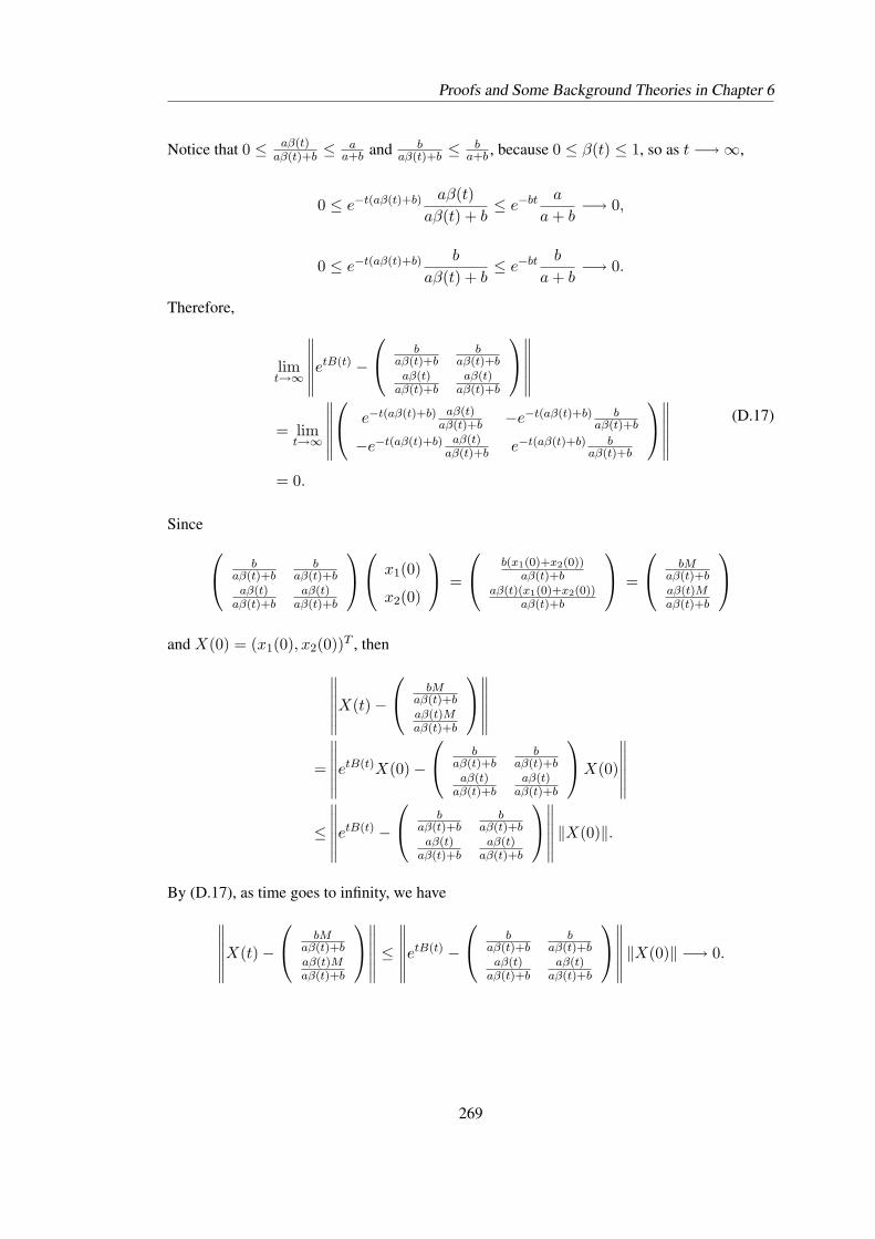
Proofs and Some Background Theories in Chapter 6
Notice that 0 ≤ aβ(t)aβ(t)+b ≤
aa+b and b
aβ(t)+b ≤b
a+b , because 0 ≤ β(t) ≤ 1, so as t −→∞,
0 ≤ e−t(aβ(t)+b) aβ(t)aβ(t) + b
≤ e−bt a
a + b−→ 0,
0 ≤ e−t(aβ(t)+b) b
aβ(t) + b≤ e−bt b
a + b−→ 0.
Therefore,
limt→∞
∥∥∥∥∥∥etB(t) −
baβ(t)+b
baβ(t)+b
aβ(t)aβ(t)+b
aβ(t)aβ(t)+b
∥∥∥∥∥∥= lim
t→∞
∥∥∥∥∥∥ e−t(aβ(t)+b) aβ(t)
aβ(t)+b −e−t(aβ(t)+b) baβ(t)+b
−e−t(aβ(t)+b) aβ(t)aβ(t)+b e−t(aβ(t)+b) b
aβ(t)+b
∥∥∥∥∥∥= 0.
(D.17)
Since baβ(t)+b
baβ(t)+b
aβ(t)aβ(t)+b
aβ(t)aβ(t)+b
x1(0)
x2(0)
=
b(x1(0)+x2(0))aβ(t)+b
aβ(t)(x1(0)+x2(0))aβ(t)+b
=
bMaβ(t)+baβ(t)Maβ(t)+b
and X(0) = (x1(0), x2(0))T , then∥∥∥∥∥∥X(t)−
bMaβ(t)+baβ(t)Maβ(t)+b
∥∥∥∥∥∥=
∥∥∥∥∥∥etB(t)X(0)−
baβ(t)+b
baβ(t)+b
aβ(t)aβ(t)+b
aβ(t)aβ(t)+b
X(0)
∥∥∥∥∥∥≤
∥∥∥∥∥∥etB(t) −
baβ(t)+b
baβ(t)+b
aβ(t)aβ(t)+b
aβ(t)aβ(t)+b
∥∥∥∥∥∥ ‖X(0)‖.
By (D.17), as time goes to infinity, we have∥∥∥∥∥∥X(t)−
bMaβ(t)+baβ(t)Maβ(t)+b
∥∥∥∥∥∥ ≤∥∥∥∥∥∥etB(t) −
baβ(t)+b
baβ(t)+b
aβ(t)aβ(t)+b
aβ(t)aβ(t)+b
∥∥∥∥∥∥ ‖X(0)‖ −→ 0.
269
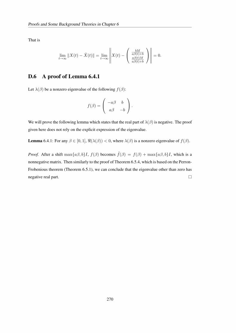
Proofs and Some Background Theories in Chapter 6
That is
limt→∞
‖X(t)− X(t)‖ = limt→∞
∥∥∥∥∥∥X(t)−
bMaβ(t)+baβ(t)Maβ(t)+b
∥∥∥∥∥∥ = 0.
D.6 A proof of Lemma 6.4.1
Let λ(β) be a nonzero eigenvalue of the following f(β):
f(β) =
−aβ b
aβ −b
.
We will prove the following lemma which states that the real part of λ(β) is negative. The proof
given here does not rely on the explicit expression of the eigenvalue.
Lemma 6.4.1: For any β ∈ [0, 1], <(λ(β)) < 0, where λ(β) is a nonzero eigenvalue of f(β).
Proof. After a shift max{aβ, b}I , f(β) becomes f(β) = f(β) + max{aβ, b}I , which is a
nonnegative matrix. Then similarly to the proof of Theorem 6.5.4, which is based on the Perron-
Frobenious theorem (Theorem 6.5.1), we can conclude that the eigenvalue other than zero has
negative real part.
270