Quadrotor Helicopter Trajectory Tracking Control,ai.stanford.edu/~gabeh/papers/GNC08_QuadTraj.pdf · Quadrotor Helicopter Trajectory Tracking Control Gabriel M. Ho mann, Steven L

Quadrotor Helicopter Trajectory Tracking Control

Gabriel M. Hoffmann∗, Steven L. Waslander†

Stanford University, Stanford, California, 94305

Claire J. Tomlin‡

University of California, Berkeley, California, 94720

The Stanford Testbed of Autonomous Rotorcraft for Multi-Agent Control (STARMAC),a fleet of quadrotor helicopters, has been developed as a testbed for novel algorithmsthat enable autonomous operation of aerial vehicles. This paper develops an autonomousvehicle trajectory tracking algorithm through cluttered environments for the STARMACplatform. A system relying on a single optimization must trade off the complexity of theplanned path with the rate of update of the control input. In this paper, a trajectorytracking controller for quadrotor helicopters is developed to decouple the two problems.By accepting as inputs a path of waypoints and desired velocities, the control input can beupdated frequently to accurately track the desired path, while the path planning occurs asa separate process on a slower timescale. To enable the use of planning algorithms that donot consider dynamic feasibility or provide feedforward inputs, a computationally efficientalgorithm using space-indexed waypoints is presented to modify the speed profile of inputpaths to guarantee feasibility of the planned trajectory and minimum time traversal of theplanned. The algorithm is an efficient alternative to formulating a nonlinear optimizationor mixed integer program. Both indoor and outdoor flight test results are presented forpath tracking on the STARMAC vehicles.

I. Introduction

The development of autonomous rotorcraft, with the capability to hover, makes possible many applica-tions for uninhabited aerial vehicles (UAVs) for which fixed wing aircraft, with more limited maneuverability,are not well suited. Examples include the close range inspection of buildings and bridges for crack formation,unexploded ordinance detection, rescue beacon tracking of first responders, RFID tracking in commercialpackage management, and wildlife monitoring. In each case, rapid trajectory generation and precise trajec-tory tracking are required to enable autonomous rotorcraft operation near obstacles in the environment.

The Stanford Testbed of Autonomous Rotorcraft for Multi-Agent Control (STARMAC) has been devel-oped as a flexible platform upon which novel algorithms can be demonstrated in real world situations withprecisely these applications in mind. By developing a multi-vehicle testbed, applications that benefit frommultiple simultaneous measurements can be developed, and methods for collision avoidance and cooperativesearch have already been developed.1,2 The choice of quadrotor helicopters ensures easy-to-use vehicles withlow maintenance requirements, and with a mass of under 3 kg, the testbed can operate in small spaces andcluttered environments with limited safety concerns. Indeed, most of STARMAC flight tests are performedon the Stanford campus, indoors and outdoors, as depicted in Figure 1.

To enable more complex missions for autonomous rotorcraft and for STARMAC in particular, this paperpresents a trajectory tracking algorithm to follow a desired path, and an algorithm for the generation ofdynamically feasible trajectories. To generate dynamically feasible trajectories, first a plan is generatedthrough the environment which satisfies collision and obstacle avoidance constraints. The planning phasecomputation is simplified by neglecting vehicle dynamic constraints, making possible real-time planning∗Ph.D. Candidate, Aeronautics and Astronautics; [email protected]. AIAA Student Member.†Postdoctoral Scholar, Aeronautics and Astronautics; [email protected]. AIAA Member.‡Professor, Department of Electrical Engineering and Computer Science; [email protected]. AIAA Member.

1 of 14

American Institute of Aeronautics and Astronautics

Figure 1. Autonomous hover at a waypoint by a quadrotor helicopter from the Stanford Testbed of AutonomousRotorcraft for Multi-Agent Control (STARMAC).

in cluttered environments using techniques such as visibility graphs3 or fast-marching.4,5 The resultingtrajectories are defined in simple geometric terms of lines and connecting curves with accompanying desiredvelocities along each segment. Then, a feasible set of inputs and travel speeds is computed, based on thecurvature of the path, given speed and acceleration constraints on the vehicles. The ability to hover enablesturning with an arbitrary radius of curvature, hence feasible trajectories are guaranteed to exist. Bothtrajectory tracking algorithms are space-indexed rather than time-indexed, enforcing the requirement thatthe obstacle-free planned path be tracked without deviation.

The trajectory tracking approach and results demonstrated on the STARMAC platform represent twosignificant advances for quadrotor vehicles. The first lies in the ability to perform accurate trajectory trackingboth indoors and out, and to do so outdoors with all sensing and computation on board the vehicles, asdemonstrated by experiments. The second lies in the novel approach to trajectory tracking for quadrotorvehicles, which exploits the hover capabilities of the quadrotor to track paths generated rapidly withoutconsideration of the vehicle dynamics. The space-indexed trajectory that results is minimum-time alongthe path that it is constrained to follow. Although the resulting travel times through the environment arenot necessarily optimal, the lower computational burden of this explicit method ensures that limited onboard resources can be used for higher level perception and planning needs. The algorithm is an efficientalternative to alternative solutions. One could formulate a nonlinear program to solve the minimum timespace-indexed optimization, requiring an iterative solution, or a mixed integer program to solve the time-indexed optimization, with exponential time complexity in the number of waypoints. The approach presentedhere requires computational time that is linear in the number of waypoints and does not need to iterate.

The paper proceeds as follows. First, related work in trajectory tracking for helicopters and the devel-opment of quadrotor testbeds is described in detail in Section II. Then, a nonlinear dynamic model of thequadrotor vehicle is presented in Section III. Section IV describes the development and flight test results ofthe quadrotor attitude control as well as the path tracking controller, which demonstrates the capability ofthe STARMAC platform to perform complex autonomous missions. Sections V then proposes an algorithmfor determining a dynamically feasible trajectory given a list of waypoints and desired velocities, and finally,simulation results of the modified trajectories in action are presented in VC.

II. Background

Autonomous trajectory tracking for rotorcraft is a widely studied problem. Recent work has focusedprimarily on nonlinear methods such as input/output linearization, where differential flatness is used toguarantee that trajectories and control inputs can be generated from an output trajectory,6 and backsteppingcontroller design7 which was used to enable acrobatic maneuvers8 for an X-Cell 0.60 size helicopter. Thebackstepping controller has been extended to include robustness considerations as well9 and in each case,flight test results were demonstrated with outdoor testbed vehicles. Although these approaches may be

2 of 14


necessary when extreme performance is required, such as in acrobatic maneuvers, the applications thatmotivate the development of STARMAC do not place such demands on the trajectory tracking control.

Many research groups are now working on quadrotors as UAV testbeds for control algorithms for au-tonomous control and sensing.10–16 A subset of these groups have been successful in performing trajectorytracking flights. One such project features the OS4 vehicle, for which a proportional-derivative (PD) controllaw led to adequate hovering capability, and an integral backstepping controller for trajectory tracking wasshown in simulation.11 A second project relies on an off-board 100 Hz Vicon state measurement system andLQR control to perform multi-vehicle maneuvers.17 The vehicles are capable of tracking slow trajectoriesthroughout an enclosed area that is visible to the Vicon system, with limited disruptions. A third project pro-posed the use of nested saturated control loops for trajectory tracking,18 for which stability guarantees wereestablished using Lyapunov theory. Experimental demonstrations were performed using the commerciallyavailable Draganfly III19 in tethered indoor flight.

In addition to research platforms, some commercially available small-scale quadrotors are becomingincreasingly capable. In particular, the MD4-200 quadrocopter from Microdrones GmbH20 is a commerciallyavailable platform that includes onboard GPS and has is capable of waypoint tracking with 2 m accuracy,outperforming many of the research projects listed above. By contrast, the results presented in this paperdemonstrate autonomous path tracking with an indoor accuracy of 10 cm and an outdoor accuracy of 50 cm.

The methodology for trajectory tracking developed for the STARMAC platform strikes a balance betweensimplicity and performance. It takes as input a path, generated by a higher level motion planner which issimplified by not needing to consider dynamic constraints, and produces a dynamically feasible sub-optimaltrajectory that the vehicle tracks using a linear controller. Although this approach is conservative in thetype of paths it generates through environments, it provides sufficient capabilities for the tasks required ofthe quadrotor testbed in most applications. The flight test results demonstrate a significant improvement incapability over previous quadrotor testbeds.

III. Vehicle Dynamics

The nonlinear dynamics of the quadrotor helicopter are those of a point mass m with moment of inertiaIb ∈ R3×3, location ρ ∈ R3 in inertial space, and angular velocity ωB ∈ R3 in the body frame. The vehicleundergoes forces F ∈ R3 in the inertial frame and moments M ∈ R3 in the body framea yielding the equationsof motion,

F = mρ (1)M = IbωB + ωB × IbωB (2)

where the total angular momentum of the rotors is assumed to be near zero, as the momentum from thecounter-rotating pairs cancels when yaw is held steady, and is small in practice. The body attitude isrepresented as a 1-2-3 Euler angle sequence with roll φ, pitch θ, and yaw ψ. A free body diagram ispresented in Figure 2, depicting the main forces and moments acting on the vehicle, including the motorthrusts and torques, gravity and aerodynamic drag.

The ith rotor contributes thrust force Ti, along local axis zRiperpendicular to the rotor planeb, which

may be tilted with respect to the body frame due to blade flapping, an aerodynamic effect described indetail in previous work.21 The thrust acts at a distance l from the center of gravity, denoted li in vectorform. Each rotor produces moments Mi in the body fixed frame. The moment is a function of the motortorque, thrust, and additional aerodynamic effects. Note that for the design of the trajectory controller, it isassumed that the disturbances in forces and moments from aerodynamic effects due to vehicle velocity canbe satisfactorily rejected in the attitude and attitude feedback control loops presented in Section IVA, andcan therefore be neglected.

The rotor thrust and reaction torque are proportional to the rotor rotation speed squared, which canbe linearized for control.21 Roll and pitch are controlled through torque generated by differential speed ofopposing pairs of rotors; rotors 2 and 4 for roll, and rotors 1 and 3 for pitch, as shown in Figure 3a. Thisyields approximately independent moments about each axis. The yaw angle is controlled through torque

aThe subscript I shall denote inertial axes in North, East, Down coordinates, with labels eN, eE, eD. The subscript B shalldenote the body reference frame, with coordinates xB,yB, zB.

bThe subscript Ri denotes to ith rotor plane reference frame.

3 of 14


Figure 2. Free body diagram of a quadrotor helicopter. The roll, pitch and yaw angles are denoted φ, θ, andψ, respectively. Motors are labeled 1 − 4, with thrust Ti and moments Mi. The force due to gravity, mg, actsin the downward direction and drag forces Db act opposite the direction of the free stream velocity eV.

(a) (b)

Figure 3. Quadrotor helicopters are controlled by varying the speeds of the rotors. (a) Pitch and roll torquesare generated independently by controlling the relative speed of rotors on opposite sides of the vehicle. (b)Yaw torque is generated by controlling the relative speed of pairs of motors, which counter-rotate to producea varying total reaction torque about the motor shafts. Vertical acceleration is controlled by the total speedof all rotors, and lateral acceleration is controlled through the pitch and roll of the aircraft.

generated by differential speed between rotors 1 and 3, which rotate one direction, and rotors 2 and 4, whichrotate the opposite direction, as shown in Figure 3b. This varies the total reaction torque about the yawaxis without affecting the roll or pitch moments, or total thrust.

The vehicle body drag force Db is a function of both vehicle and wind speed, and acceleration due togravity is denoted g. The total force F is the summation of all contributing forces,

F = −Dbev +mgeD +4∑i=1

(−TiRRi,IzRi) (3)

where RRi,I is the rotation matrix from the plane of rotor i to inertial coordinatesc. Similarly, the totalmoment, M, is,

M =4∑i=1

(Mi + li × (−TiRRi,BzRi)) (4)

where RRi,B is the rotation matrix from the plane of rotor i to body coordinates. Note that the dragforce was neglected in computing the moments acting on the vehicle, as it was found to cause a negligibledisturbance on the total moment over the flight regime of interest compared to other aerodynamic moments.Combining Equations (2) with (3) and (4) yields a full set of nonlinear dynamics for the quadrotor vehicles.

cThe notation RA,B shall refer to rotation matrices from coordinate system A to B throughout.

4 of 14


IV. Trajectory Tracking Control

The proposed control law tracks line segments connecting sequences of waypoints at a desired velocity. Todesign the trajectory tracking control law, the strong attitude angle control authority of quadrotor helicopterscan be exploited. This section proceeds by first presenting an attitude control law with the ability to trackrapidly varying commands. The altitude control law is given in previous work, using feedback linearizationand acceleration feedback.21 Next, the path tracking control law is presented, which uses the attitudecontroller to orient the vehicle’s thrust to produce the desired lateral acceleration.

A. Attitude Control

The equations of motion are approximately decoupled about each attitude axis, so control inputs about eachaxis, uφ, uθ, and uψ, can be implemented independently. This is an accurate assumption when the angularvelocities are low and the attitude angles are within approximately ±30◦. The inputs for each axis can thenbe combined to generate u1 through u4, for motors 1 through 4,

u1 = −uθ + uψ + uz

u2 = uφ − uψ + uz

u3 = uθ + uψ + uz

u4 = −uφ − uψ + uz

(5)

In controlling each attitude angle, the time delay in thrust must be included in the model. It is wellapproximated as a first order delay, as experimentally verified.21 Linearizing Equation (4), the resultingtransfer function for the roll axis is

Φ(s)Uφ(s)

=Iφ/l

s2(τs+ 1)(6)

where Iφ is the component of Ib for the roll axis, l is once again the lever arm of the rotors about the centerof mass, and τ is the thrust time delay, which was experimentally determine to be 0.1 sec for STARMAC.The transfer functions for the pitch and yaw axes are similarly computed.

Although a standard proportional-integral-derivative (PID) controller has been shown to perform ade-quately,22 control design using root locus techniques revealed that adding an additional zero, using angularacceleration feedback, allowed the gains to be significantly increased, yielding higher bandwidth. Also notethat aerodynamic disturbance torques are directly measured by errors in the angular acceleration. Theresulting control law,

C(s) = kdds2 + kds+ kp +

kis

(7)

was tuned to provide substantially faster and more accurate performance than previously possible. TheLaplace transform of the control input is then,

U(s) = C(s)(Θref (s)−Θ(s)) (8)

The implementation of this control law requires some consideration. First, the required angular accel-eration signal must be computed by finite differencing the rate gyroscope data, a step which can amplifynoise. However, in implementation, it was found that the signal resulting from a single difference using76 Hz measurements from rate gyroscope chips was sufficiently clean for use in the controller. Second, toimplement this control law, C(s) acts on the error signal to provide reference command tracking capability.To enable this, it was necessary to process the reference command using a low pass digital filter to computeboth first and second derivatives.

In practice, the controller is able to track rapidly varying reference commands, as shown in Figure 4,with root mean square (RMS) error of 0.65◦ in each axis. Aggressive flights have been flown frequently, withtypically up to 15◦ of bank angle. The controller has been flown up to its programmed limit of 30◦ withoutapparent degradation in performance.

5 of 14


0 5 10 15 20 25 30 35 40 45 50

−10

0

10

Time (s)

Rol

l (de

g)

0 5 10 15 20 25 30 35 40 45 50

−10

0

10

Time (s)

Pitc

h (d

eg)

0 5 10 15 20 25 30 35 40 45 50

−10

0

10

Time (s)

Yaw

(de

g)

−2 0 20

200

400

600

Roll Tracking Error (deg)

Sam

ples

−2 0 20

200

400

600

Pitch Tracking Error (deg)

Sam

ples

−2 0 20

200

400

600

Yaw Tracking Error (deg)

Sam

ples

Figure 4. Attitude control results from a flight test a STARMAC quadrotor, accurately tracking a time varyingreference command. The dashed line is the reference command, the solid line is the measured vehicle attitudeangle.

Figure 5. Vehicle path definition. While the quadrotor travels along segment Pi from waypoint xdi to xd

i+1, itapplies along track and cross track control inputs uat and uct to follow the path segment.

B. Path Tracking Control

With an attitude controller of sufficient bandwidth defined, it is possible to develop a path tracker thatgenerates attitude reference commands, ignoring the fast dynamics of the attitude angles.

A path, P ∈ N ×R3, is defined by a sequence of N desired waypoints, xdi and desired speeds of travel vdialong path segment Pi connecting waypoint i to i + 1, as depicted in Figure 5. Let ti be the unit tangentvector in the direction of travel along the track from xdi to xdi+1, and ni be the unit normal vector to thetrack. Then, given the current position x(t), the cross track error ect and along track error rate eat are,

ect = (xdi − x(t)) · niect = −v(t) · nieat = vdi − v(t) · ti

(9)

Note that only the along track error rate is considered, and depends only the velocity of the vehicle. Thisis done so that the resulting controller does not attempt to catch up or slow down for scheduled waypoints,but simply proceeds along the track matching the desired velocity as closely as possible.

A trajectory tracking controller was implemented by closing the loop on along track velocity and crosstrack error. This is essentially piecewise PI control in the along track direction, and PID control in the cross

6 of 14


track direction.

uat = Katpeat +Kati

t∫0

eatdt

uct = Kctpect +Kctdect +Kcti

t∫0

ectdt

(10)

Transition from segment i to i + 1 occurs when the vehicle crosses the line segment normal to the path atthe end of the segment. Upon completion of Pi, the integrators were reset because the along track and crosstrack error integrals reject different disturbances. Note than when the transition angle from one segment tothe next is sufficiently small, as occurs for low curvature paths, the integrators need not be reset.

The controller defined in Equation 7 was implemented on the STARMAC platform in both indoor andoutdoor settings, for which results are presented in Figures 6 and 7, respectively. The indoor results demon-strate tracking errors of under 10cm throughout the box shaped trajectory, and show the largest overshootwhen switching from one track to the next, as the desired direction of travel suddenly switches by 90◦. Forthe outdoor flight tests, the gains on the cross track and along track controllers were reduced significantly,and the resulting errors increased to ±0.5 m. Lower gains were used due to increased oscillations when inhover condition outside, and may be attributed to either significant levels of wind gust disturbances or tothe decreased position update rate from 15 Hz for the indoor positioning system to 10 Hz for the carrierphase differential GPS solution. Further investigation is required to isolate the true source of this drop inperformance.

−0.6 −0.4 −0.2 0 0.2 0.4 0.6

−0.6

−0.4

−0.2

0

0.2

0.4

East (m)

Nor

th (

m)

Figure 6. Tracking a trajectory indoors, at 0.5 m/s, with an error of under 0.1 m. An overhead webcam isused to provide 15 Hz position updates simulating GPS data.

One thing to note in the above flight test results, in particular in the case of the indoor trajectory, isthe effect of direction changes in the trajectory to be tracked. Since the trajectory controller as defined inEquation 10 has no sense of the curvature of the desired trajectory, significant overshoot on sharp corners isinevitable. This can cause concern in constrained environments if, for example the changes in direction arerequired to avoid obstacles or other vehicles in the environment. Section V now presents modifications to thetrajectory to be tracked that do incorporate path curvature and vehicle dynamics when making transitionsfrom one waypoint to the next, enabling more precise tracking performance.

V. Time Optimal Feasible Trajectory

Given a planned sequence of desired waypoints, the desired speed profile for the quadrotor must begenerated in a dynamically feasible manner. Although the speed profile can be determined at the time of

7 of 14


−4 −2 0 2 40

2

4

6

8

10

East (m)

Nor

th (

m)

Figure 7. Tracking a trajectory outdoors, at 2.0 m/s, with an error of under 0.5 m. GPS is used for position,and nominal winds were measured at 5-10 mph.

trajectory generation, this step increases the complexity of trajectory planning and many algorithms withlow complexity can quickly generate paths, but cannot guarantee dynamic feasibility. Examples includeusing A∗ with visibility graphs,23 and fast marching5 with gradient descent, as shown in Figure 8. In orderto render the trajectory dynamically feasible, this section presents a method to compute a space-indexedspeed profile that traverses the sequence of waypoints in minimum time while satisfying acceleration andspeed constraints. This algorithm runs in O(N) time, where N is the number of waypoints.

This method starts by generating a finer sampling of waypoints than the examples in Section B, whichdefines a space-indexed path, x ∈ RN×2, with a curvature that can be numerically estimatedd. For compu-tational efficiency, the algorithm assumes acceleration constraints apply separately in the along track andcross track directions. First, the cross track acceleration constraint is satisfied by computing a maximumallowable speed at every waypoint, using the approximate path curvature. Second, the optimal time speedprofile is computed that satisfies piecewise linear along track acceleration constraints, as well as the minimumof the desired speed and of the allowable speed from the previous step.

A. Cross Track Acceleration Constraint Satisfaction

The cross track acceleration act,i at waypoint xi = (xi, yi) is a function of the velocity vct,i at xi and theradius of curvature ri,

act,i =v2i

ri(11)

Constraining the cross track acceleration to be of magnitude less than amax results in a maximum allowablevelocity vi,allow at xi,

vi,allow ≤√amaxri (12)

To determine ri, waypoints xi−1, xi, and xi+1 are used to define a circle through those points. This circle isassumed to have curvature ri, a valid assumption when the the waypoints are finely spaced relative to theircurvature. Waypoints xi−1 and xi define a first line, and points xi and xi+1 define a second line, with slopesma and mb respectively. The intersection of the perpendicular lines through their midpoints is at the centerof the circle. The slopes are

ma =yi − yi−1

xi − xi−1, mb =

yi+1 − yixi+1 − xi

(13)

dNote that the variable x is reused by abuse of notation, in order to greatly simplify the derivation in this section.

8 of 14


0 2 4 6 8 10 120

1

2

3

4

5

6

7

8

0 2 4 6 8 100

1

2

3

4

5

6

7

8

(a) (b)

Figure 8. (a) Visibility Graph, with shortest path highlighted, and waypoints sampled with a spacing of 0.2units. (b) Fast marching potential function with steepest descent path highlighted.

Solving for the intersection yields the center point xci ,

xci =mamb(yi−1 − yi+1) +mb(xi−1 + xi)−ma(xi + xi+1)

2(mb −ma)(14)

This can be substituted into the equation for the line to obtain yci . Equation (13) can be substituted into(14) to obtain a form that is numerically well behaved. This yields

xci =(x2i−1 + y2

i−1)(yi − yi+1) + (x2i + y2

i )(yi+1 − yi−1) + (x2i+1 + y2

i+1)(yi−1 − yi)ci

(15)

yci =(x2i−1 + y2

i−1)(xi+1 − xi) + (x2i + y2

i )(xi−1 − xi+1) + (x2i+1 + y2

i+1)(xi − xi−1)ci

(16)

whereci = 2(yi+1(xi − xi−1) + yi(xi−1 − xi+1) + yi−1(xi+1 − xi)) (17)

Note that ci should be precomputed as it’s value is zero for any straight line segment where the radius ofcurvature is infinite. Otherwise, the centerpoint can be computed using (15). The radius ri is the norm of thevector connecting xi and the center. The direction of the curve can be computed for finite ri using the signof the cross product of the first and second line segments. Now, with a speed limit imposed by accelerationconstraints, vi,allow, at every waypoint, the speed plan and feedforward acceleration can be computed forthe path, as presented next.

B. Time Optimal Speed and Acceleration Plan

The speed at every point is constrained by both the desired velocity vi,max as defined by the pre-path, whichmust be feasible for the vehicle to fly, and by the constraint imposed for the cross track acceleration constraint,vi,allow. At every point, the minimum of these two constraints must be satisfied. Let the maximum velocityallowed at each space-indexed point be,

vi = min(vi,max, vi,allow) (18)

This section derives the algorithm to determine the speed profile, v ∈ RN , and acceleration profiles, aat ∈ RNand act ∈ RN , that satisfy these constraints.

Consider piecewise constant along track acceleration aat,i between waypoints i and i + 1. The speed atthe next waypoint vi+1 given current speed vi and time between waypoints ∆t is

vi+1 = vi + aat,i∆t (19)

9 of 14


Let the along track position of waypoint i be si, measured from the beginning of the path, i.e., ||xi+1−xi||2 =si+1 − si. To determine ∆t, integrate (19).

12aat,i∆t2 + vi∆t+ (si − si+1) = 0 (20)

Solving for ∆t yields

∆t =−vi ±

√v2i − 2aat,i(si − si+1)aat,i

(21)

Substituting (21) into (19),

vi+1 =√v2i − 2aat,i(si − si+1) (22)

Note that only the positive root in (21) has a physical interpretation because the speeds must be positive.Solving for the acceleration to achieve a given change in speed over a given distance,

aat,i =v2i − v2

i+1

2(si − si+1)(23)

Algorithm 1 Velocity Plan Sweep(v0, s, v, amax)v1 ← v0

for i = 1 to N doaat,i ← min

(amax,

v2i−(vi+1)2

2(si−si+1)

)if aat,i > 0 thenvi+1 ←

√v2i − 2aat,i(si − si+1)

∆ti ←−vi+√v2i−2aat,i(si−si+1)

aat,i

elseif vi > vi+1 thenvi+1 ← vi+1

aat,i ←v2i−v

2i+1

2(si−si+1)

∆ti ←−vi+√

(v2i−2aat,i(si−si+1))

aat,i

elsevi+1 ← viaat,i ← 0∆ti ← si+1−si

vi

end ifend if

end forreturn v, a, ∆t

Next, the algorithm to compute the time optimal plan is explained. It operates in five steps. First, allalong track positions are stored in s and all maximum speeds are stored in v. Second, to prepare for sweepingthrough the points from the end to the beginning, these arrays are reversed in time, and s is negated. Third,to satisfy the minimum acceleration constraint the sweeping algorithm, defined in Algorithm 1 and describedbelow, is run on the reversed data with v0 = vN to generate an along track acceleration plan, a, such thataat,i > −amax ∀ i. Third, to retain the minimum acceleration constraint from the previous step, v is setto the resulting v. Fourth, to prepare for sweeping through the points from beginning to end, the arraysare again reversed in time, and s is negated. Fifth, to enforce the maximum acceleration constraint, thesweeping algorithm is run on this data, with v0 = v1, to generate a such that aat,i < amax ∀ i. In thissweep, aat,i < −amax is not possible due to the speed limits imposed by the previous, reverse sweep. Oncethese reverse and forward sweeps have been completed, the acceleration constraints and speed constraintsare satisfied.

The sweeping algorithm, Algorithm 1, operates by incrementing through the waypoints. At waypoint i,it first determines if it is possible to accelerate between xi and xi+1. If it can accelerate, it accelerates as fast

10 of 14


as required, or saturates at amax. If it cannot accelerate, it next checks if it must slow down to satisfy vi+1.If it must, it slows down to that speed, using whatever acceleration necessary, even if using aat,i < −amax ifrequired. Note that it only violates amax to slow down. If it does not need to slow down, then it holds thecurrent speed. Finally, it returns the computed speed profile, v, acceleration profile, a, and time profile, ∆t.Note that ∆t must be computed, because the algorithm is space-indexed.

Using this algorithm, the time optimal speed and along track acceleration can be computed. The crosstrack acceleration required to achieve this path has magnitude vi/r2

i , with the sign equal to that of the thirdcomponent of the cross product of tangent vectors ti−1 and ti. The computed feedforward accelerationscan then be superimposed with the feedback control law, (10), to control the quadrotor to track the desiredtrajectory at the time-optimal speed.

C. Application to Example Problems

0 2 4 6 8 10 120

0.5

1

1.5

2

2.5

Spe

ed (m

/s)

Position on Path (m)

vplan

vlim

0 2 4 6 8 10 12−1.5

−1

−0.5

0

0.5

1

1.5

Nom

inal

Acc

el (m

/s2 )


uat

uct

0 5 10 150

5

10

15

Pos

ition

(m)

Time (s)

0 5 10 150

0.5

1

1.5

2

Spe

ed (m

/s)

Time (s)

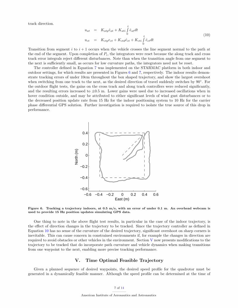
Figure 9. Results from optimizing the visibility graph based path, yielding a 13.6 sec plan. When the pathchanges direction around obstacle corners, the vehicle must slow down to a safe speed, accelerate laterally,then speed up again.

The time optimal sweeping algorithm was applied to the two examples of path planning algorithmsgiven in the beginning of this section, and shown in Figure 8. All experiments were run using a 3.4 GHzPentium IV computer and the time to compute the plan demonstrated that this algorithm is negligible, asexpected by its O(n) time complexity. The plans demonstrate the ability of the algorithm to capture thenecessary information to produce a time-optimal trajectory.

1. Visibility Graph

Consider the path generated using a A* to find the shortest path through a visibility graph,23 shown inFigure 8a. The generation of the shortest path required under 20 ms using Matlab. However, this methodignored dynamic constraints, which would require the quadrotor to slow to a halt at sharp corners. To runthe optimum time sweeping algorithm, the shortest path was discretized at 0.2 m increments, resulting ina computation time of under 1 ms to run optimum time sweeping. The results are shown in Figure 9. Theminimum time to traverse the path under acceleration and speed constraints was 13.6 sec.

One drawback to the presented approach is that corners may be cut, depending on the fineness of thediscretization, a problem common to many path planning algorithms. However, the computational cost for

11 of 14


choosing a sufficiently fine discretization is low, given the low run time of the sweeping algorithm and soan arbitrary precision may be used to avoid obstacles. The effect of increasing the precision of the spacediscretization is that it increases the total time to complete the trajectory, as the velocity slows to zero ateach turn in the underlying desired path. In some problem formulations, it is desirable for corners to be cut,if there is sufficient margin in the definition of obstacles used in generating the original plan. This allowssharp corners in the paths to be traversed without stopping, which is only advantageous when there aresharp corners in the path as in the case of the visibility graph. Fast marching, on the other hand, does notsuffer from this trade off.

2. Fast Marching

0 5 10 150

0.5

1

1.5

2

2.5

Spe

ed (m

/s)


vplan

vlim

0 5 10 15−1.5

−1

−0.5

0

0.5

1

1.5

Nom

inal

Acc

el (m

/s2 )


uat

uct

0 5 10 150

5

10

15

Pos

ition

(m)

Time (s)

0 5 10 150

0.5

1

1.5

2

Spe

ed (m

/s)

Time (s)

Figure 10. Results from optimizing the fast marching based path, yielding a 13.8 sec plan. Although this pathis longer than the visibility graph based path, there are no corners, so the average speed is faster.

Consider the path generated using fast marching with the planar wave approximation,5 shown in Fig-ure 8b. This method, using a discrete grid, propagates the cost to reach the goal from the goal outward,increasing with distance. Close proximity to obstacles increases this cost, resulting in the refraction of thewave front around surfaces. Using the resulting cost map, gradient descent is used to find the best path tothe target, according to the cost map. In the example shown, the complete path finding algorithm againran in under 20 ms. Due to the aversion to obstacles, this cost map is not exactly the time to the goal–thevehicle is penalized for being close to obstacles. To run the optimum time sweeping algorithm, the fastmarching path was discretized at 0.2 m increments again, and resulted in a computation time of under 1 ms.The results are shown in Figure 10. The minimum time to traverse the path under acceleration and speedconstraints was 13.8 sec.

The results for fast marching differ from those of the visibility graph. Although the aversion to obstaclesresults in smoother paths, the paths are always longer than the visibility graph. As a result, sometimes thevisibility graph is faster, and sometimes the fast marching path is faster. The aversion to obstacles causesfast marching to tend to avoid going through small gaps when possible, which is advantageous if there arewinding corners, but hurts performance if there is a simple gap. The resulting minimum time accelerationcommands for the fast marching path varied much more smoothly than for the visibility graph, due to a lackof corners. Although the maximum velocity constraint due to cross track acceleration was active for moretime than it was for the visibility graph path, the minimum values were not as low, so the average speeds

12 of 14


were close to equal for the two examples.In both examples, the computation time to find a path through the environment was low because dynamic

constraints were first ignored to find the path, and then included by the optimum time sweeping algorithm.By separately considering vehicle dynamics and path plans, the overall paths are not optimal. However,given the already good paths, the optimum time sweeping algorithm generates a control input and speedplan that traverses the path in minimum time. This algorithm can be run online in real-time with thefeedback controller of Section B.

VI. Conclusions

Autonomous rotorcraft can make possible many potential applications for uninhabited aerial vehicles.To enable more complex missions for autonomous quadrotors, and for STARMAC in particular, this paperpresented a trajectory tracking algorithm to follow a desired path, and an algorithm for the generation ofdynamically feasible trajectories. The trajectory tracking algorithm used has been experimentally demon-strated to track a path indoors with 10 cm accuracy and outdoors with 50 cm accuracy. The dynamicallyfeasible trajectory generation algorithm separated the plan generation for obstacle avoidance from the com-putation of dynamically feasible travel speeds and control inputs. In doing so, it is possible to find thetime optimal inputs to follow a given path with little computational burden. Simulations demonstrate theaccurate computation of these control inputs, and the fast run time on the computer.

In future work, it would be interesting to investigate the possibility of generating trajectories that slightlymodify the location of space indexed waypoints to improve the minimum travel speed for the worst offendingsegments along the path. It may also be possible to incorporate knowledge of the obstacle locations in thevelocity determination to ensure slower, more precise tracking when in constrained spaces. The proposedalgorithm will be next be implemented and tested on the STARMAC platform, and flight test results fromthese experiments will be included in the final version of the paper. With reliable tracking of trajectoriesachieved, the STARMAC platform will be ready to embark on many of the applications envisaged for it,including multi-vehicle collision avoidance and cooperative target localization in unknown environments.

Acknowledgments

The authors would like to thank Vijay Pradeep, Haomiao Huang and Michael Vitus for their manycontributions to the STARMAC project, and in particular, Vijay Pradeep, for his work on the fast-marchingalgorithm.

References

1Hoffmann, G. M., Waslander, S. L., and Tomlin, C. J., “Distributed Cooperative Search using Information-Theoretic Costsfor Particle Filters with Quadrotor Applications,” Proceedings of the AIAA Guidance, Navigation, and Control Conference,Keystone, CO, August 2006.

2Waslander, S. L., Multi-agent system design for aerospace applications, Ph.D. thesis, Stanford University, Stanford, CA,USA, 2007.

3Asand, T., Asano, T., Guibas, L., Hershberger, J., and Imai, H., “Visibility of Disjoint Polygons,” Algorithmica, Vol. 1,1986, pp. 49–63.

4Kimmel, R. and Sethian, J., “Computing geodesic paths on manifolds,” Proceedings of National Academy of Sciences,Vol. 95, 1998, pp. 8431–8435.

5Osher, S. and Fedkiw, R., Level Set Methods and Dynamic Implicit Surfaces, Springer-Verlag, New York, NY, USA,2002.

6Koo, T. J. and Sastry, S., “Output Tracking Control Design of a Helicopter Model Based on Approximate Linearization,”Proceedings of the 37th IEEE Conference on Decision and Control , Tampa Bay, Florida, USA, December 1998.

7Frazzoli, E., Dahleh, M., and Feron, E., “Trajectory tracking control design for autonomous helicopters using a backstep-ping algorithm,” AACC American Control Conference, 2000, pp. 4102 – 4107.

8Gavrilets, V., Martinos, I., Mettler, B., and Feron, E., “Flight test and simulation results for an autonomous aerobatichelicopter,” Vol. 2, 2002, pp. 8C3–1–8C3–6, DOI: 10.1109/DASC.2002.1052943.

9Mahony, R. and Hamel, T., “Robust trajectory tracking for a scale model autonomous helicopter,” International Journalof Robust and Nonlinear Control , Vol. 14, No. 12, 2004, pp. 1035–1059, DOI: 10.1002/rnc.931.

10Altug, E., Ostrowski, J. P., and Taylor, C. J., “Quadrotor Control Using Dual Camera Visual Feedback,” In Proceedingsof the IEEE International Conference on Robotics and Automation, Taipei, Taiwan, Sept 2003, pp. 4294–4299.

13 of 14


11Bouabdallah, S., Murrieri, P., and Siegwart, R., “Towards Autonomous Indoor Micro VTOL,” Autonomous Robots,Vol. 18, No. 2, March 2005, pp. 171–183.

12Guenard, N., Hamel, T., and Moreau, V., “Dynamic modeling and intuitive control strategy for an X4-flyer,” In Pro-ceedings of the International Conference on Control and Automation, Budapest, Hungary, June 2005, pp. 141–146.

13Escareno, J., Salazar-Cruz, S., and Lozano, R., “Embedded control of a four-rotor UAV,” Proceedings of the AACCAmerican Control Conference, Minneapolis, MN, June 2006, pp. 3936–3941.

14Nice, E. B., Design of a Four Rotor Hovering Vehicle, Master’s thesis, Cornell University, 2004.15Park, S., Won, D., Kang, M., Kim, T., Lee, H., and Kwon, S., “RIC (Robust Internal-loop Compensator) Based Flight

Control of a Quad-Rotor Type UAV,” Proceedings of the IEEE/RSJ International Conference on Intelligent Robotics andSystems, Edmonton, Alberta, August 2005.

16Pounds, P., Mahony, R., and Corke, P., “Modelling and Control of a Quad-Rotor Robot,” In Proceedings of the Aus-tralasian Conference on Robotics and Automation, Auckland, New Zealand, 2006.

17Culligan, K., Valenti, M., Kuwata, Y., and How, J. P., “Three-Dimensional Flight Experiments Using On-Line Mixed-Integer Linear Programming Trajectory Optimization,” Proceedings of the AACC American Control Conference, New York,NY, July 2006, pp. 5322–5327.

18Salazar-Cruz, S., Palomino, S., and Lozano, R., “Trajectory tracking for a four rotor mini-aircraft,” Proceedings of theIEEE Conference on Decision and Control , Seville, Spain, December 2005, pp. 2505–2510.

19“DraganFly-Innovations DraganFlyer III,” 2006, http://www.rctoys.com.20Microdrones GmbH MD4-200 quadrotor helicopter , 2008, http://www.microdrones.com/news waypoint navigation.html.21Hoffmann, G. M., Huang, H., Waslander, S. L., and Tomlin, C. J., “Quadrotor Helicopter Flight Dynamics and Control:

Theory and Experiment,” Proceedings of the AIAA Guidance, Navigation, and Control Conference, Hilton Head, SC, August2007.

22Waslander, S. L., Hoffmann, G. M., Jang, J. S., and Tomlin, C. J., “Multi-Agent Quadrotor Testbed Control Design:Integral Sliding Mode vs. Reinforcement Learning,” In Proceedings of the IEEE/RSJ International Conference on IntelligentRobotics and Systems 2005 , Edmonton, Alberta, August 2005, pp. 468–473.

23Latombe, J.-C., Robot Motion Planning, Kluwer Academic Publishers, Boston, MA, USA, 1991.

14 of 14


Documents

Quadrotor Helicopter Trajectory Tracking Control,ai.stanford.edu/~gabeh/papers/GNC08_QuadTraj.pdf · Quadrotor Helicopter Trajectory Tracking Control Gabriel M. Ho mann, Steven L