Sliding Mode Approach to Control Quadrotor Using …cdn.intechopen.com/...mode...control_quadrotor_using_dynamic_inve… · A typical model of a quadrotor helicopter ... Sliding Mode

1

Sliding Mode Approach to Control Quadrotor Using Dynamic Inversion

Abhijit Das, Frank L. Lewis and Kamesh Subbarao Automation and Robotics Research Institute

The University of Texas at Arlington USA

1. Introduction

Nowadays unmanned rotorcraft are designed to operate with greater agility, rapid maneuvering, and are capable of work in degraded environments such as wind gusts etc. The control of this rotorcraft is a subject of research especially in applications such as rescue, surveillance, inspection, mapping etc. For these applications, the ability of the rotorcraft to maneuver sharply and hover precisely is important (Koo and Sastry 1998). Rotorcraft control as in these applications often requires holding a particular trimmed state; generally hover, as well as making changes of velocity and acceleration in a desired way (Gavrilets, Mettler, and Feron 2003). Similar to aircraft control, rotorcraft control too involves controlling the pitch, yaw, and roll motion. But the main difference is that, due to the unique body structure of rotorcraft (as well as the rotor dynamics and other rotating elements) the pitch, yaw and roll dynamics are strongly coupled. Therefore, it is difficult to design a decoupled control law of sound structure that stabilizes the faster and slower dynamics simultaneously. On the contrary, for a fixed wing aircraft it is relatively easy to design decoupled standard control laws with intuitively comprehensible structure and guaranteed performance (Stevens and F. L. Lewis 2003). There are many different approaches available for rotorcraft control such as (Altug, Ostrowski, and Mahony 2002; Bijnens et al. 2005; T. Madani and Benallegue 2006; Mistler, Benallegue, and M'Sirdi 2001; Mokhtari, Benallegue, and Orlov 2006) etc. Popular methods include input-output linearization and back-stepping. The 6-DOF airframe dynamics of a typical quadrotor involves the typical translational and rotational dynamical equations as in (Gavrilets, Mettler, and Feron 2003; Castillo, Lozano, and Dzul 2005; Castillo, Dzul, and Lozano 2004). The dynamics of a quadrotor is essentially a simplified form of helicopter dynamics that exhibits the basic problems including under-actuation, strong coupling, multi-input/multi-output, and unknown nonlinearities. The quadrotor is classified as a rotorcraft where lift is derived from the four rotors. Most often they are classified as helicopters as its movements are characterized by the resultant force and moments of the four rotors. Therefore the control algorithms designed for a quadrotor could be applied to a helicopter with relatively straightforward modifications. Most of the papers (B. Bijnens et al. 2005; T. Madani and Benallegue 2006; Mokhtari, Benallegue, and Orlov 2006) etc. deal with either input-output linearization for decoupling pitch yaw roll or back-stepping to deal with the under-actuation problem. The problem of coupling in the

www.intechopen.com

Challenges and Paradigms in Applied Robust Control 4

yaw-pitch-roll of a helicopter, as well as the problem of coupled dynamics-kinematic underactuated system, can be solved by back-stepping (Kanellakopoulos, Kokotovic, and Morse 1991; Khalil 2002; Slotine and Li 1991). Dynamic inversion (Stevens and F. L. Lewis 2003; Slotine and Li 1991; A. Das et al. 2004) is effective in the control of both linear and nonlinear systems and involves an inner inversion loop (similar to feedback linearization) which results in tracking if the residual or internal dynamics is stable. Typical usage requires the selection of the output control variables so that the internal dynamics is guaranteed to be stable. This implies that the tracking control cannot always be guaranteed for the original outputs of interest. The application of dynamic inversion on UAV’s and other flying vehicles such as missiles, fighter aircrafts etc. are proposed in several research works such as (Kim and Calise 1997; Prasad and Calise 1999; Calise et al. 1994) etc. It is also shown that the inclusion of dynamic neural network for estimating the dynamic inversion errors can improve the controller stability and tracking performance. Some other papers such as (Hovakimyan et al. 2001; Rysdyk and Calise 2005; Wise et al. 1999; Campos, F. L. Lewis, and Selmic 2000) etc. discuss the application of dynamic inversion on nonlinear systems to tackle the model and parametric uncertainties using neural nets. It is also shown that a reconfigurable control law can be designed for fighter aircrafts using neural net and dynamic inversion. Sometimes the inverse transformations required in dynamic inversion or feedback linearization are computed by neural network to reduce the inversion error by online learning. In this chapter we apply dynamic inversion to tackle the coupling in quadrotor dynamics which is in fact an underactuated system. Dynamic inversion is applied to the inner loop, which yields internal dynamics that are not necessarily stable. Instead of redesigning the output control variables to guarantee stability of the internal dynamics, we use a sliding mode approach to stabilize the internal dynamics. This yields a two-loop structured tracking controller with a dynamic inversion inner loop and an internal dynamics stabilization outer loop. But it is interesting to notice that unlike normal two loop structure, we designed an inner loop which controls and stabilizes altitude and attitude of the quadrotor and an outer loop which controls and stabilizes the position (x,y) of the quadrotor. This yields a new structure of the autopilot in contrast to the conventional loop linear or nonlinear autopilot. Section 2 of this chapter discusses the basic quadrotor dynamics which is used for control law formulation. Section 3 shows dynamic inversion of a nonlinear state-space model of a quadrotor. Sections 4 discuss the robust control method using sliding mode approach to stabilize the internal dynamics. In the final section, simulation results are shown to validate the control law discussed in this chapter.

2. Quadrotor dynamics

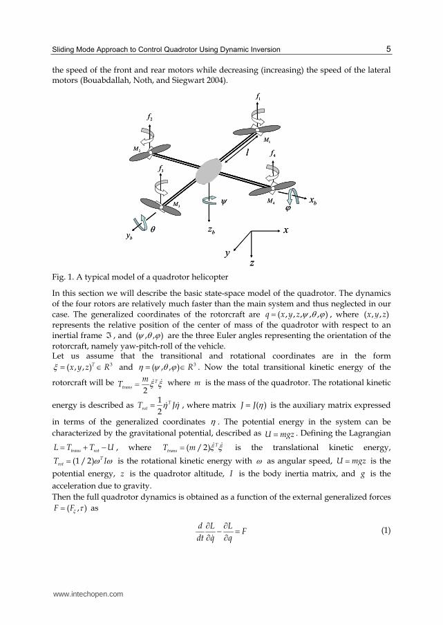
Fig. 1 shows a basic model of an unmanned quadrotor. The quadrotor has some basic advantage over the conventional helicopter. Given that the front and the rear motors rotate counter-clockwise while the other two rotate clockwise, gyroscopic effects and aerodynamic torques tend to cancel in trimmed flight. This four-rotor rotorcraft does not have a swash-plate (P. Castillo, R. Lozano, and A. Dzul 2005). In fact it does not need any blade pitch control. The collective input (or throttle input) is the sum of the thrusts of each motor (see Fig. 1). Pitch movement is obtained by increasing (reducing) the speed of the rear motor while reducing (increasing) the speed of the front motor. The roll movement is obtained similarly using the lateral motors. The yaw movement is obtained by increasing (decreasing)

www.intechopen.com

Sliding Mode Approach to Control Quadrotor Using Dynamic Inversion 5

the speed of the front and rear motors while decreasing (increasing) the speed of the lateral motors (Bouabdallah, Noth, and Siegwart 2004).

Fig. 1. A typical model of a quadrotor helicopter

In this section we will describe the basic state-space model of the quadrotor. The dynamics of the four rotors are relatively much faster than the main system and thus neglected in our case. The generalized coordinates of the rotorcraft are ( , , , , , )q x y z , where ( , , )x y z

represents the relative position of the center of mass of the quadrotor with respect to an inertial frame , and ( , , ) are the three Euler angles representing the orientation of the rotorcraft, namely yaw-pitch-roll of the vehicle. Let us assume that the transitional and rotational coordinates are in the form 3( , , )Tx y z R and 3( , , ) R . Now the total transitional kinetic energy of the

rotorcraft will be 2

Ttrans

mT where m is the mass of the quadrotor. The rotational kinetic

energy is described as 12

TrotT J , where matrix ( )J J is the auxiliary matrix expressed

in terms of the generalized coordinates . The potential energy in the system can be characterized by the gravitational potential, described as U mgz . Defining the Lagrangian

trans rotL T T U , where ( / 2) TtransT m is the translational kinetic energy,

(1 / 2) TrotT I is the rotational kinetic energy with as angular speed, U mgz is the

potential energy, z is the quadrotor altitude, I is the body inertia matrix, and g is the acceleration due to gravity. Then the full quadrotor dynamics is obtained as a function of the external generalized forces

( , )F F as

d L L

Fdt q q

(1)

l

1f

1M

2M

2f

3M

3f

4M

4f

bxbz

by

x

yz

l

1f

1M

2M

2f

3M

3f

4M

4f

bxbz

by

x

yz

www.intechopen.com


The principal control inputs are defined as follows. Define

0

0RF

u

(2)

where u is the main thrust and defined by

1 2 3 4u f f f f (3)

and if ’s are described as 2i i if k , where ik are positive constants and i are the angular

speed of the motor i . Then F can be written as

RF RF (4)

where R is the transformation matrix representing the orientation of the rotorcraft as

c c s s s

R c s s s c s s s c c c s

c s c s s s s c c s c c

(5)

The generalized torque for the variables are

(6)

where

4 1 2 3 41

( )iM

i

c f f f f (7)

2 4( )f f l (8)

3 1( )f f l (9)

Thus the control distribution from the four actuator motors of the quadrotor is given by

1

2

3

4

1 1 1 1

0 0

0 0

f

u f

l l f

l l f

c c c c f

C

(10)

where l is the distance from the motors to the center of gravity, iM is the torque produced

by motor iM , and c is a constant known as force-to-moment scaling factor. So, if a required thrust and torque vector are given, one may solve for the rotor force using (10).

www.intechopen.com


The final dynamic model of the quadrotor is described by (11)-(14),

0

0 Rm F

mg

(11)

1

( )2

TdJ J J

dt (12)

,dJ J C

dt (13)

,J C (14)

where,

sin

cos sin

cos cosRF u , auxiliary Matrix TJ J T IT with

sin 0 1

cos sin cos 0

cos cos sin 0

T .

Now finally the dynamic model of the quadrotor in terms of position , ,x y z and rotation ( , , ) is written as,

0 sin1

0 cos sin

cos cos

x

y um

z g

(15)

( , , ) ( , , )f g (16)

where,

( , , )

y z p

x x

pz x

y y

x y

z

I I J

I I

JI If

I I

I I

I

,

0 0

( , , ) 0 0

0 0

x

y

z

l

I

lg

I

l

I

, 1u R and

3R are the

control inputs, , ,x y zI are body inertia, pJ is propeller/rotor inertia and 2 4 1 3 .

Thus, the system is the form of an under-actuated system with six outputs and four inputs.

www.intechopen.com


Comment 2.1: In this chapter we considered a generalized state space model of quadrotor derived from Lagrangian dynamics. Design autopilot with actual Lagrangian model of quadrotor is discussed in (Abhijit Das, Frank Lewis, and Kamesh Subbarao 2009).

3. Partial feedback linearization for Quadrotor model

Dynamic inversion (Stevens and F. L. Lewis 2003) is an approach where a feedback linearization loop is applied to the tracking outputs of interest. The residual dynamics, not directly controlled, is known as the internal dynamics. If the internal dynamics are stable, dynamic inversion is successful. Typical usage requires the selection of the output control variables so that the internal dynamics is guaranteed to be stable. This means that tracking cannot always be guaranteed for the original outputs of interest. In this chapter we apply dynamic inversion to the system given by (15) and (16) to achieve station-keeping tracking control for the position outputs ( , , , )x y z . Initially we select the convenient output vector ( , , , )diy z which makes the dynamic inverse easy to find. Dynamic inversion now yields effectively an inner control loop that feedback linearizes the system from the control ( , , , )diu u to the output ( , , , )diy z . Note that the output contains attitude parameters as well as altitude of the quadrotor. Note however that diy is not the desired system output. Moreover, dynamic inversion generates a specific internal dynamics, as detailed below, which may not always be stable. Therefore, a second outer loop is designed to generate the required values for ( , , , )diy z in terms of the values of the desired tracking output ( , , , )x y z . An overall Lyapunov proof guarantees stability and performance. The following background is required. Consider a nonlinear system of the form

, qq f q u (17)

where mqu R is the control input and nq R is state vector. The technique of designing the

control input u using dynamic inversion involves two steps. First, one finds a state transformation ( )z z q and an input transformation ( , )q qu u q v

so that the nonlinear

system dynamics is transformed into an equivalent linear time invariant dynamics of the form

z az bv (18)

where ,n n n ma R b R are constant matrices with v is known as new input to the linear system. Secondly one can design v easily from the linear control theory approach such as pole placement etc. To get the desired linear equations (18), one has to differentiate outputs until input vector diu appears. The procedure is known as dynamic inversion.

3.1 Dynamic inversion for inner loop

The system, (15)→(16) is an underactuated system if we consider the states ( , , , , , )x y z as

outputs and T

diu u as inputs. To overcome these difficulties we consider

four outputs ( , , , )diy z which are used for feedback linearization. Differentiating the output vector twice with respect to the time we get from (15) and (16) that,

www.intechopen.com


di di di diy M E u (19)

where,

4

y z p

x x

pdi z x

y y

x y

z

g

I I J

I I

JM I I

I I

I I

I

,

4 4

(1 / )cos cos 0 0 0

0 0 0

0 0 0

0 0 0

x

di

y

z

m

l

I

lE

I

l

I

The number 8r of differentiation required for an invertible diE is known as the relative degree of the system and generally 12r n ; if r n then full state feedback linearization is achieved if diE is invertible. Note that for multi-input multi-output system, if number of outputs is not equal to the number of inputs (under-actuated system), then diE becomes non-square and is difficult to obtain a feasible linearizing input diu . It is seen that for non-singularity of diE , 0 , 90 . The relative degree of the system is calculated as 8 whereas the order of the system is 12 . So, the remaining dynamics ( 4) which does not come out in the process of feedback linearization is known as internal dynamics. To guarantee the stability of the whole system, it is mandatory to guarantee the stability of the internal dynamics. In the next section we will discuss how to control the internal dynamics using a PID with a feed-forward acceleration outer loop. Now using (19) we can write the desired input to the system

1di di di diu E M v (20)

which yields

di diy v (21)

where, T

di zv v v v v . This system is decoupled and linear. The auxiliary input div

is designed as described below.

3.2 Design of linear controller

Assuming the desired output to the system is T

d d d d dy z , the linear controller

div is designed in the following way

1 2

1 2

1 2

1 2

( ) ( )

( ) ( )

( ) ( )

( ) ( )

z zd d dz

d d d

di

d d d

d d d

z K z z K z zv

K Kvv

v K K

v K K

(22)

www.intechopen.com


where, 1 2, ,....K K etc. are positive constants so that the poles of the error dynamics arising from (23) and (24) are in the left half of the s plane. For hovering control, dz and d are chosen depending upon the designer choice.

3.3 Defining sliding variable error

Let us define the state error 1

T

d d d de z z and a sliding mode error as

1 1 1 1r e e (23)

where, 1 is a diagonal positive definite design parameter matrix. Common usage is to select 1 diagonal with positive entries. Then, (23) is a stable system so that 1e is bounded as long as the controller guarantees that the filtered error 1r is bounded. In fact it is easy to show (F. Lewis, Jagannathan, and Yesildirek 1999) that one has

11 1 1

min 1

,( )

re e r (24)

Note that 1 1 1 0e e defines a stable sliding mode surface. The function of the controller to be designed is to force the system onto this surface by making 1r small. The parameter 1 is selected for a desired sliding mode response

11 1 1( ) (0)te t e e (25)

We now focus on designing a controller to keep 1r small. From (23),

1 1 1 1r e e (26)

Adding an integrator to the linear controller given in (22), and now we can rewrite (22) as

1 1 2 1 3 10d

t

di div y K e K e K r dt (27)

where, , , ,d

T

di d d d dy z and ( , , , ) 0zi i i i iK diag K K K K , 1,2,3, 4i .

Now using equation (20) and (27) we can rewrite the equation (19) in the form of error dynamics as

1 1 1 2 1 3 10

0t

e K e K e K r dt (28)

Thus equation (26) becomes

1 1 1 2 1 3 1 1 10

t

r K e K e K r dt e (29)

If we choose 1 1 2 1( ),K R K R , then equation (29) will look like

1 1 3 10

t

r Rr K r dt (30)

www.intechopen.com


Note that 0R is also a diagonal matrix.

4. Sliding mode control for internal dynamics

The internal dynamics (Slotine and Li 1991) for the feedback linearizes system given by

sinu

xm

(31)

cos sinu

ym

(32)

For the stability of the whole system as well as for the tracking purposes, ,x y should be bounded and controlled in a desired way. Note that the altitude z of the rotorcraft a any given time t is controlled by (20),(22). To stabilize the zero dynamics, we select some desired d and d such that ( , )x y is bounded. Then that ,d d can be fed into (22) as a reference. Using Taylor series expansion about some nominal values

d , d and considering up to first order terms

* * *

* * *

* * *

sin sin cos ( )

cos cos sin ( )

sin sin cos ( )

d d d d d

d d d d d

d d d d d

(33)

Using (33) on (31) we get

* * *sin cos ( )d d d d

ux

m (34)

* * * * * *cos sin ( ) sin cos ( )d d d d d d d d

uy

m (35)

For hovering of a quadrotor, assuming the nominal values * 0d , * 0d , (31) and (32) becomes

d

ux

m (36)

d

uy

m (37)

Define the state error

2

T

d de x x y y (38)

and the sliding mode error for the internal dynamics as

2 2 2 2r e e (39)

www.intechopen.com


where, 2

is a diagonal positive definite design parameter matrix with similar characteristic of 1 . Also

22 2 2

min 2

,( )

re e r (40)

Therefore according to (40), designing a controller to keep 2r small will guarantee that

2e and 2e are small. Differentiating 2r we get

2 2 2 2r e e (41)

Let the choice of the control law is as follows

11 12 13 2 20

( ) sgn( ) , 0t

d d d d x x

mx c x x c x x c r dt r

u (42)

21 22 23 2 20

( ) sgn( ) , 0t

d d d d y y

my c y y c y y c r dt r

u (43)

where,

111

21

00

0

cC

c,

122

22

00

0

cC

c,

133

23

00

0

cC

c and

00

0x

y

.

Combining the equations (36) to (43)

2 1 2 2 2 3 2 20

sgn( ) 0t

e C e C e C r dt r (44)

Therefore

2 1 2 2 2 3 2 2 2 20

sgn( )t

r C e C e C r dt r e (45)

Let

1 2 0C S (46)

2 2 0C S (47)

Therefore

2 2 0 2 2 0 2 3 2 2 2 20

sgn( )t

r S e S e C r dt r e (48)

2 0 2 3 2 20

sgn( )t

r S r C r dt r (49)

www.intechopen.com


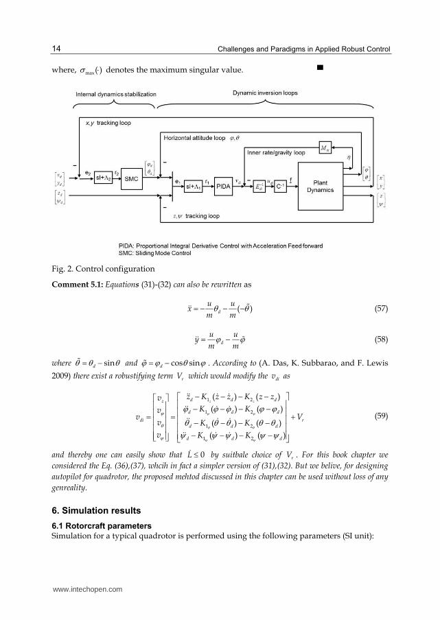
5. Controller structure and stability analysis

The overall control system has two loops and is depicted in Fig. 2. The following theorem details the performance of the controller. Definition 5.1: The equilibrium point ex is said to be uniformly ultimately bounded (UUB) if there

exist a compact set nS R so that for all 0x S there exist a bound B and a time 0( , )T B x such that 0( ) ( )ex t x t B t t T .

Theorem 5.1: Given the system as described in (15) and (16) with a control law shown in Fig. 2. and

given by (20), (27), (42) , (43) . Then, the tracking errors 1r and 2r and thereby 1e and 2e are UUB

if (53) and (54) are satisfied and can be made arbitrarily small with a suitable choice of gain

parameters. According to the definition given by (23) of 1r and (39) of 2r , this guarantees that 1e

and 2e are UUB since

1

1

2

2

11

min 1 min 1

22

min 2 min 2

0

0

r

r

r

r

bre b

bre b

(50)

where min i is the minimum singular value of , 1,2i i .

Proof: Consider the Lyapunov function

1 1 1 2 1 2 1 2 1 2 2 2

0 0 0 0

1 1 1 12 2 2 2

t t t tT T T TL r P r r Q r r dt P r dt r dt Q r dt (51)

with symmetric matrices 1 2 1 2, , , 0P P Q Q

Therefore, by differentiating L we will get the following

1 1 1 1 1 3 1 1 2 1 2 1 0 20 0

2 1 3 2 2 2 2 2 1 20 0

sgn( )

t tT T T

t tT T T

L r P Rr r P K r dt r P r dt r Q S r

r Q C r dt r Q r dt r Q r

(52)

Define,

2 1 3P P K (53)

2 1 3Q Q C (54)

then integration term vanishes.

1 1 1 2 1 0 2 2 1 2sgn( )T T TL r P Rr r Q S r r Q r (55)

The Equation (55) can be written as

2 2max 1 1 max 1 0 2 max 1 2( ) ( ) ( ) 0L P R r Q S r Q r (56)

www.intechopen.com


where, max( ) denotes the maximum singular value. ▀

Fig. 2. Control configuration

Comment 5.1: Equations (31)-(32) can also be rewritten as

( )d

u ux

m m (57)

d

u uy

m m (58)

where sind and cos sind . According to (A. Das, K. Subbarao, and F. Lewis

2009) there exist a robustifying term rV which would modify the div as

1 2

1 2

1 2

1 2

( ) ( )

( ) ( )

( ) ( )

( ) ( )

z zd d dz

d d d

di r

d d d

d d d

z K z z K z zv

K Kvv V

v K K

v K K

(59)

and thereby one can easily show that 0L by suitbale choice of rV . For this book chapter we

considered the Eq. (36),(37), whcih in fact a simpler version of (31),(32). But we belive, for designing

autopilot for quadrotor, the proposed mehtod discussed in this chapter can be used without loss of any

genreality.

6. Simulation results

6.1 Rotorcraft parameters

Simulation for a typical quadrotor is performed using the following parameters (SI unit):

www.intechopen.com


1

1 0 0

0 1 0

0 0 1

M ;

5 0 0

0 5 0

0 0 15

J ; 9.81g .

6.2 Reference trajectory generation

As outlined in Refs (Hogan 1984; Flash and Hogan 1985), a reference trajectory is derived that minimizes the jerk (rate of change of acceleration) over the time horizon. The trajectory ensures that the velocities and accelerations at the end point are zero while meeting the position tracking objective. The following summarizes this approach:

2 3 41 2 3 4 5( ) 2 3 4 5

x x x x xdx t a a t a t a t a t (60)

Differentiating again,

2 32 3 4 5( ) 2 6 12 20

x x x xdx t a a t a t a t (61)

As we indicated before that initial and final velocities and accelerations are zero; so from Eqs. (60) and (61) we can conclude the following:

23

24

25

1

0 3 4 5

0 6 12 20

x

x

x

x f f

f f

f f

d t t a

t t a

t t a

(62)

Where, 0

3/fx d d fd x x t . Now, solving for coefficients

123

24

25

1

3 4 5 0

6 12 20 0

x

x

x

f f x

f f

f f

a t t d

a t t

a t t

(63)

Thus the desired trajectory for the x direction is given by

0

3 4 53 4 5( )

x x xd dx t x a t a t a t (64)

Similarly, the reference trajectories for the y and z directions are gives by Eq. (65) and Eq. (66) respectively.

0

3 4 53 4 5( )

y y yd dy t y a t a t a t (65)

0

3 4 53 4 5( )

z z zd dz t z a t a t a t (66)

The beauty of this method lying in the fact that more demanding changes in position can be accommodated by varying the final time. That is acceleration/torque ratio can be controlled smoothly as per requirement. For example, Let us assume at 0,t

00dx and at 10t sec, 10

fdx . Therefore xd 0.01 and the trajectory is given by Eq. (67) and shown in Fig. 3 for various desired final positions.

3 4 5( ) 0.1 0.015 0.0006dx t t t t (67)

www.intechopen.com


Fig. 3. Example trajectory simulation for different final positions

6.3 Case 1: From initial position at 0,5,10 to final position at 20, 5,0

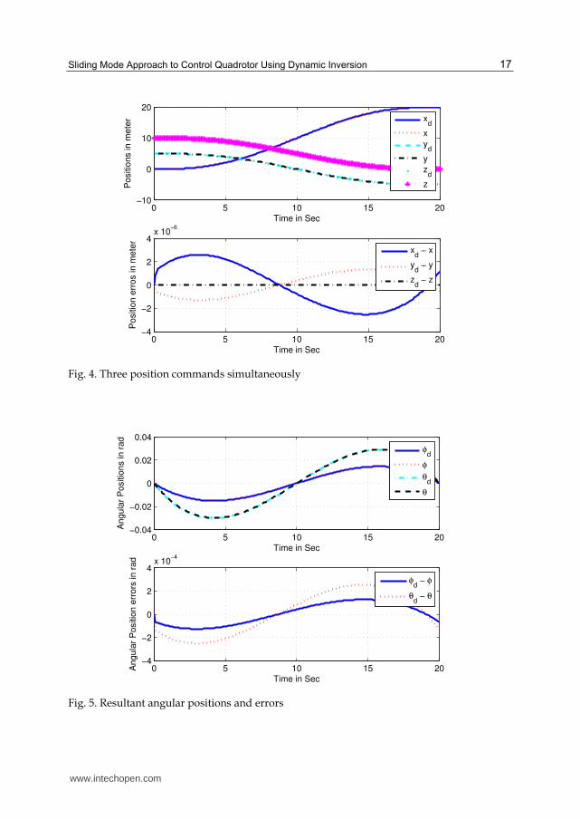
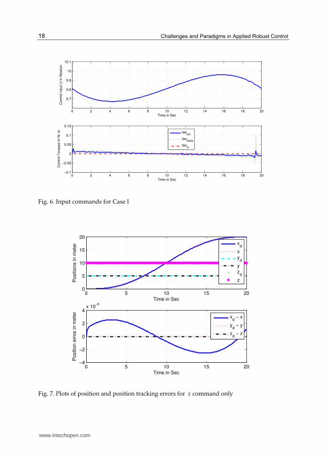
Figure 4 describes the controlled motion of the quadrotor from its initial position 0,5,10 to final position 20, 5,0 for a given time (20 seconds). The actual trajectories ( ), ( ), ( )x t y t z t match exactly their desired values ( ), ( ), ( )d d dx t y t z t respectively nearly exactly. The errors along the three axes are also shown in the same figure. It can be seen that the tracking is almost perfect as well as the tracking errors are significantly small. Figure 5 describes the attitude of the quadrotor , along with their demands ,d d and attitude errors in radian. Again the angles match their command values nearly perfectly. Figure 6 describes the control input requirement which is very much realizable. Note that as described before the control requirement for yaw angle is 0

and it is seen from Fig. 6.

6.4 Case 2: From initial position at 0,5,10 to final position at 20,5,10

Figures 7-8 illustrates the decoupling phenomenon of the control law. Fig. 7 shows that ( )x t follows the command ( )dx t nearly perfectly unlike ( )y t and ( )z t are held their initial values. Fig. 8 shows that the change in x does not make any influence on . The corresponding control inputs are also shown in Fig. 9 and due to the full decoupling effect it is seen that

is almost zero. The similar type of simulations are performed for y and z directional motions separately and similar plots are obtained showing excellent tracking.

0 2 4 6 8 100

5

10

15

20

25

30

35

40

Time in Seconds

x d (t) i

n m

eter

Example Reference Trajectory

www.intechopen.com

�� %"�

Fig. 4. Three position commands simultaneously

Fig. 5. Resultant angular positions and errors

0 5 10 15 20−10

0

10

20

Time in Sec

Positio

ns in m

ete

r

xd

x

yd

y

zd

z

0 5 10 15 20−4

−2

0

2

4x 10

−6

Time in Sec

Positio

n e

rros in m

ete

r

xd − x

yd − y

zd − z

0 5 10 15 20−0.04

−0.02

0

0.02

0.04

Time in Sec

Angula

r P

ositio

ns in r

ad

φd

φ

θd

θ

0 5 10 15 20−4

−2

0

2

4x 10

−4

Time in Sec

Angula

r P

ositio

n e

rrors

in r

ad

φd − φ

θd − θ

www.intechopen.com

�� %#

Fig. 6. Input commands for Case I

Fig. 7. Plots of position and position tracking errors for � command only

0 2 4 6 8 10 12 14 16 18 20

9.7

9.8

9.9

10

10.1

Time in Sec

Co

ntr

ol in

pu

t U

in

Ne

wto

n

0 2 4 6 8 10 12 14 16 18 20−0.1

−0.05

0

0.05

0.1

0.15

Time in Sec

Co

ntr

ol T

orq

ue

s I

n N

−m

taophi

taotheta

taosi

0 5 10 15 200

5

10

15

20

Time in Sec

Positio

ns in m

ete

r

xd

x

yd

y

zd

z

0 5 10 15 20−4

−2

0

2

4x 10

−6

Time in Sec

Positio

n e

rros in m

ete

r

xd − x

yd − y

zd − z

www.intechopen.com

�� %$�

Fig. 8. Angular variations due to change in �

Fig. 9. Input commands for variation in � (Case II)

0 5 10 15 20−0.04

−0.02

0

0.02

0.04

Time in Sec

Angula

r P

ositio

ns in r

ad

φd

φ

θd

θ

0 5 10 15 20−4

−2

0

2

4x 10

−4

Time in Sec

Angula

r P

ositio

n e

rrors

in r

ad

φd − φ

θd − θ

0 5 10 15 209.81

9.812

9.814

9.816

9.818

Time in Sec

Contr

ol in

put U

in N

ew

ton

0 5 10 15 20−0.05

0

0.05

0.1

0.15

Time in Sec

Contr

ol T

orq

ues In N

−m

taophi

taotheta

taosi

www.intechopen.com

�� '&

'�&��,�� "��

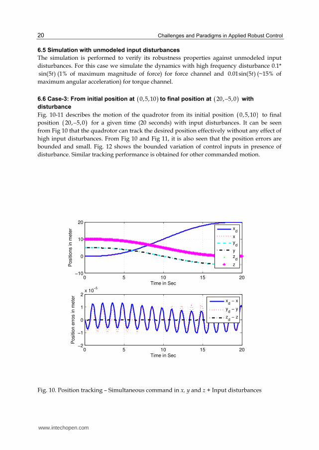
The simulation is performed to verify its robustness properties against unmodeled input

disturbances. For this case we simulate the dynamics with high frequency disturbance 0.1*

sin(5 )� (1% of maximum magnitude of force) for force channel and 0.01sin(5 )� (~15% of

maximum angular acceleration) for torque channel.

'�'��-�*�+�� ( )0,5,10 ��!�� ( )−20, 5,0 �,��

��"��

Fig. 10811 describes the motion of the quadrotor from its initial position ( )0,5,10 to final

position ( )−20, 5,0 for a given time (20 seconds) with input disturbances. It can be seen

from Fig 10 that the quadrotor can track the desired position effectively without any effect of

high input disturbances. From Fig 10 and Fig 11, it is also seen that the position errors are

bounded and small. Fig. 12 shows the bounded variation of control inputs in presence of

disturbance. Similar tracking performance is obtained for other commanded motion.

Fig. 10. Position tracking – Simultaneous command in �� and + Input disturbances

0 5 10 15 20−10

0

10

20

Time in Sec

Positio

ns in m

ete

r

xd

x

yd

y

zd

z

0 5 10 15 20−2

−1

0

1

2x 10

−5

Time in Sec

Positio

n e

rros in m

ete

r

xd − x

yd − y

zd − z

www.intechopen.com

�� '%�

Fig. 11. Angular variations, errors and velocities (with input disturbances)

Fig. 12. Force and torque input variations (with input disturbances)

0 5 10 15 20−0.04

−0.02

0

0.02

0.04

Time in Sec

Angula

r P

ositio

ns in r

ad

φd

φ

θd

θ

0 5 10 15 20−4

−2

0

2

4x 10

−4

Time in Sec

Angula

r P

ositio

n e

rrors

in r

ad

φd − φ

θd − θ

0 5 10 15 20

9.7

9.8

9.9

10

10.1

10.2

Time in Sec

Contr

ol in

put U

in N

ew

ton

0 5 10 15 20−0.4

−0.2

0

0.2

0.4

Time in Sec

Contr

ol T

orq

ues In N

−m

taophi

taotheta

taosi

www.intechopen.com


7. Conclusion

Sliding mode approach using input-output linearization to design nonlinear controller for a quadrotor dynamics is discussed in this Chapter. Using this approach, an intuitively structured controller was derived that has an outer sliding mode control loop and an inner feedback linearizing control loop. The dynamics of a quadrotor are a simplified form of helicopter dynamics that exhibits the basic problems including under-actuation, strong coupling, multi-input/multi-output. The derived controller is capable of deal with such problems simultaneously and satisfactorily. As the quadrotor model discuss in this Chapter is similar to a full scale unmanned helicopter model, the same control configuration derived for quadrotor is also applicable for a helicopter model. The simulation results are presented to demonstrate the validity of the control law discussed in the Chapter.

8. Acknowledgement

This work was supported by the National Science Foundation ECS-0801330, the Army Research Office W91NF-05-1-0314 and the Air Force Office of Scientific Research FA9550-09-1-0278.

9. References

Altug, Erdinc, James P. Ostrowski, and Robert Mahony. 2002. Control of a Quadrotor Helicopter Using Visual Feedback ID - 376. In . Washington DC, Virginia, June.

B. Bijnens, Q. P. Chu, G. M. Voorsluijs, and J. A. Mulder. 2005. AIAA Guidance, Navigation, and Control Conference and Exhibit. In . San Francisco, California.

Bijnens, B., Q. P. Chu, G. M. Voorsluijs, and J. A. Mulder. 2005. Adaptive Feedback Linearization Flight Control for a Helicopter UAVID - 199.

Bouabdallah, Samir, AndrÂ´e Noth, and Roland Siegwart. 2004. International Conference on Intelligent Robots and Systems. In , 3:2451-2456. Sendal, Japan: IEEE.

Calise, A. J., B. S. Kim, J. Leitner, and J. V. R. Prasad. 1994. Helicopter adaptive flight control using neural networks. In . Lake Buena Vista, FL.

Campos, J., F. L. Lewis, and C. R. Selmic. 2000. Backlash Compensation in Discrete Time Nonlinear Systems Using Dynamic Inversion by Neural Networks. In . San Francisco, CA.

Castillo, P., A. Dzul, and R. Lozano. 2004. Real-time Stabilization and Tracking of a Four-Rotor Mini Rotorcraft. IEEE Transaction on Control System Technology 12: 510-516.

Castillo, P., R. Lozano, and A. Dzul. 2005. Modelling and Control of Mini Flying Machines. Springer-Verlag.

Das, A., T. Garai, S. Mukhopadhyay, and A. Patra. 2004. Feedback Linearization for a Nonlinear Skid-To-Turn Missile Model. First India annual conference, Proceedings of

the IEEE INDICON 2004: 586-589. Das, A., K. Subbarao, and F. Lewis. 2009. Dynamic inversion with zero-dynamics

stabilisation for quadrotor control. Control Theory & Applications, IET 3, no. 3 (March): 303 - 314.

www.intechopen.com


Das, Abhijit, Frank Lewis, and Kamesh Subbarao. 2009. Backstepping Approach for Controlling a Quadrotor Using Lagrange Form Dynamics. Journal of Intelligent and

Robotic Systems 56, no. 1-2 (4): 127-151. doi:10.1007/s10846-009-9331-0. Flash, T., and N. Hogan. 1985. The Coordination of Arm Movements: an Experimentally

Confirmed Mathematical Model. Journal of Neuro Science 5: 1688-1703. Gavrilets, V., B. Mettler, and E. Feron. 2003. Dynamic Model for a Miniature Aerobatic

Helicopter. MIT-LIDS report LIDS-P-2580. Hogan, N. 1984. Adaptive Control of Mechanical Impedance by Coactivation of Antagonist

Muscles. IEEE Transaction of Automatic Control 29: 681-690. Hovakimyan, N., F. Nardi, A. J. Calise, and H. Lee. 2001. Adaptive Output Feedback Control

of a Class of Nonlinear Systems Using Neural Networks. International Journal of

Control 74: 1161-1169. Kanellakopoulos, I., P. V. Kokotovic, and A. S. Morse. 1991. Systematic Design of Adaptive

Controllers for Feedback Linearizable Systems. IEEE Transaction of Automatic

Control 36: 1241-1253. Khalil, Hassan K. 2002. Nonlinear Systems. 3rd ed. Upper Saddle River, N.J: Prentice

Hall. Kim, B. S., and A. J. Calise. 1997. Nonlinear flight control using neural networks. Journal of

Guidance Control Dynamics 20: 26-33. Koo, T. J., and S. Sastry. 1998. Output tracking control design of a helicopter model based on

approximate linearization. In Proceedings of the 37th Conference on Decision and

Control. Tampa, Florida: IEEE. Lewis, F., S. Jagannathan, and A. Yesildirek. 1999. Neural Network Control of Robot

Manipulators and Nonlinear Systems. London: Taylor and Francis. Mistler, V., A. Benallegue, and N. K. M'Sirdi. 2001. Exact linearization and non- interacting

control of a 4 rotors helicopter via dynamic feedback. In 10th IEEE Int. Workshop on

Robot-Human Interactive Communication. Paris. Mokhtari, A., A. Benallegue, and Y. Orlov. 2006. Exact Linearization and Sliding Mode

Observer for a Quadrotor Unmanned Aerial Vehicle. International Journal of Robotics

and Automation 21: 39-49. P. Castillo, R. Lozano, and A. Dzul. 2005. Stabilization of a Mini Rotorcraft Having Four

Rotors. IEEE Control System Magazine 25: 45-55. Prasad, J. V. R., and A. J. Calise. 1999. Adaptive nonlinear controller synthesis and

flight evaluation on an unmanned helicopter. In . Kohala Coast-Island of Hawaii, USA.

Rysdyk, R., and A. J. Calise. 2005. Robust Nonlinear Adaptive Flight Control for Consistent Handling Qualities. IEEE Transaction of Control System Technology 13: 896-910.

Slotine, Jean-Jacques, and Weiping Li. 1991. Applied Nonlinear Control. Prentice Hall. Stevens, B. L., and F. L. Lewis. 2003. Aircraft Simulation and Control. Wiley and Sons. T. Madani, and A. Benallegue. 2006. Backstepping control for a quadrotor helicopter. In .

Beijing, China.

www.intechopen.com


Wise, K. A., J. S. Brinker, A. J. Calise, D. F. Enns, M. R. Elgersma, and P. Voulgaris. 1999. Direct Adaptive Reconfigurable Flight Control for a Tailless Advanced Fighter Aircraft. International Journal of Robust and Nonlinear Control 9: 999-1012.

www.intechopen.com

Challenges and Paradigms in Applied Robust ControlEdited by Prof. Andrzej Bartoszewicz

ISBN 978-953-307-338-5Hard cover, 460 pagesPublisher InTechPublished online 16, November, 2011Published in print edition November, 2011

InTech EuropeUniversity Campus STeP Ri Slavka Krautzeka 83/A 51000 Rijeka, Croatia Phone: +385 (51) 770 447 Fax: +385 (51) 686 166www.intechopen.com

InTech ChinaUnit 405, Office Block, Hotel Equatorial Shanghai No.65, Yan An Road (West), Shanghai, 200040, China

Phone: +86-21-62489820 Fax: +86-21-62489821

The main objective of this book is to present important challenges and paradigms in the field of applied robustcontrol design and implementation. Book contains a broad range of well worked out, recent application studieswhich include but are not limited to H-infinity, sliding mode, robust PID and fault tolerant based controlsystems. The contributions enrich the current state of the art, and encourage new applications of robustcontrol techniques in various engineering and non-engineering systems.

How to referenceIn order to correctly reference this scholarly work, feel free to copy and paste the following:

Abhijit Das, Frank L. Lewis and Kamesh Subbarao (2011). Sliding Mode Approach to Control Quadrotor UsingDynamic Inversion, Challenges and Paradigms in Applied Robust Control, Prof. Andrzej Bartoszewicz (Ed.),ISBN: 978-953-307-338-5, InTech, Available from: http://www.intechopen.com/books/challenges-and-paradigms-in-applied-robust-control/sliding-mode-approach-to-control-quadrotor-using-dynamic-inversion

Documents

Sliding Mode Approach to Control Quadrotor Using …cdn.intechopen.com/...mode...control_quadrotor_using_dynamic_inve… · A typical model of a quadrotor helicopter ... Sliding Mode