Downwash-Aware Trajectory Planning for Large Quadrotor Teams

James A. Preiss, Wolfgang Honig, Nora Ayanian, and Gaurav S. Sukhatme

Abstract— We describe a method for formation-change tra-jectory planning for large quadrotor teams in obstacle-richenvironments. Our method decomposes the planning probleminto two stages: a discrete planner operating on a graph repre-sentation of the workspace, and a continuous refinement thatconverts the non-smooth graph plan into a set of Ck-continuoustrajectories, locally optimizing an integral-squared-derivativecost. We account for the downwash effect, allowing safe flight indense formations. We demonstrate the computational efficiencyin simulation with up to 200 robots and the physical plausibilitywith an experiment with 32 nano-quadrotors. Our approachcan compute safe and smooth trajectories for hundreds ofquadrotors in dense environments with obstacles in a fewminutes.

I. INTRODUCTION

Trajectory planning is a fundamental problem in multi-robot systems. Given a set of robots with known initiallocations and a set of goal locations, the task is to find aone-to-one goal assignment and a set of continuous functionsthat move each robot from its start position to its goal, whileavoiding collisions and respecting dynamic limits. Trajectoryplanning is a core subproblem of various applications includ-ing search-and-rescue, inspection, and delivery. In this workwe address the unlabeled case; in the labeled case the goalassignment is given.

A large body of work has addressed this problem withvaried discrete and continuous formulations. However, noexisting solution simultaneously satisfies the goals of com-pleteness, physical plausibility, optimality in time or energyusage, and good computational performance. In this work,we present a method that attempts to balance these goals.

Our method uses a graph-based planner to compute asolution for a discretized version of the problem, and thenrefines this solution into smooth trajectories in a separate,decoupled optimization stage. We directly take the downwasheffect of quadrotors into account, preserving safety duringdense formation flights. Furthermore, our method is completewith respect to the resolution of the discretization, and lo-cally optimal with respect to an energy-minimizing integral-squared-derivative objective function. We also present ananytime iterative refinement scheme that improves the trajec-tories within a given computational budget. We support user-specified smoothness constraints and provide simulationswith up to 200 robots and a physical experiment with 32quadrotors, see Fig. 1.

All authors are with the Department of Computer Science, University ofSouthern California, Los Angeles, CA, USA.

Email: japreiss, whoenig, ayanian, gaurav@usc.eduThis work was partially supported by the ONR grants N00014-16-1-2907

and N00014-14-1-0734, and the ARL grant W911NF-14-D-0005.

Fig. 1. Long exposure of 32 Crazyflie nano-quadrotors flying through awall with windows, viewed from the edge of the wall.

II. RELATED WORK

A simple approach to multi-robot motion planning is torepurpose a single-robot planner and represent the Cartesianproduct of the robots’ configuration spaces as a singlelarge joint configuration space [1]. Robot-robot collisions arerepresented as configuration-space obstacles. However, thehigh-dimensional search space is computationally infeasiblefor large teams.

Many works have approached the problem from a graphsearch perspective [2], [3]. These methods are adept atdealing with maze-like environments and scenarios with highcongestion. Some represent the search graph implicitly [4],so they are not always restricted to a predefined set ofpoints in configuration space. However, directly interpretinga graph plan as a trajectory results in a piecewise linearpath, requiring the robot to fully stop at each graph vertexto maintain dynamic feasibility. It is possible to use theseplanners to resolve ordering conflicts and refine the outputfor execution on robots [5].

Some authors have solved the formation change problemin a continuous setting [6], [7], but methods are often tightlycoupled, solving one large optimization problem in whichthe decision variables define all robots’ trajectories. Theseapproaches are typically demonstrated on smaller teams anddo not scale up to the size of team in which we are interested.Others decouple the problem but do not support the level ofsmoothness in our solution [8], and the authors do not showresults on large teams. The method of [9] is computationallyfast, but offsets the different trajectories in time, resulting inmuch longer time durations. Velocity profile methods [10]handle kinodynamic constraints well but are not able to fullyexploit free space in the environment. Collision-avoidanceapproaches [11], [12] let each robot plan its trajectory inde-pendently and resolve conflicts in real time when impendingcollisions are detected. These methods scale well, and their

robustness against disturbances is appealing. However, theydo not provide any means to optimize the trajectories forobjectives such as time or energy use, and they are poorlysuited to problems in maze-like environments.

Spline-based refinement of waypoint plans was describedin [13] and [14]. Our method builds upon these worksby adding support for three-dimensional ellipsoidal robots,environmental obstacles, and an anytime refinement stageto further improve the plan after generating an initial setof smooth trajectories. We demonstrate that our iterativerefinement produces trajectories with significantly smootherdynamics.

III. APPROACH

We start by introducing the robot model, which is requiredto model the downwash effect. We then formalize the prob-lem statement and outline our approach. In later sections, wewill discuss each part of our approach in detail.

A. Robot Model

As aerial vehicles, quadrotors have a six-dimensionalconfiguration space. However, as shown in [15], quadrotorsare differentially flat in the flat outputs (x, y, z, ψ), wherex, y, z is the robot’s position in space and ψ its yaw angle(heading). Differential flatness implies that the control inputsneeded to move the robot along a trajectory in the flat outputsare algebraic functions of the flat outputs and a finite numberof their derivatives. Furthermore, in many applications, aquadrotor’s yaw angle is unimportant and can be fixed atψ = 0. We therefore focus our efforts on planning trajectoriesin three-dimensional Euclidean space.

While some multi-robot planning work has consideredsimplified dynamics models such as kinematic agents [5]or double-integrators [6], our method produces trajectorieswith arbitrary smoothness up to a user-defined derivative.This goal is motivated by [15], where it was shown thata continuous fourth derivative of position is necessary forphysically plausible quadrotor trajectories, because it ensuresthat the quadrotor will not be asked to change its motorspeeds instantaneously.

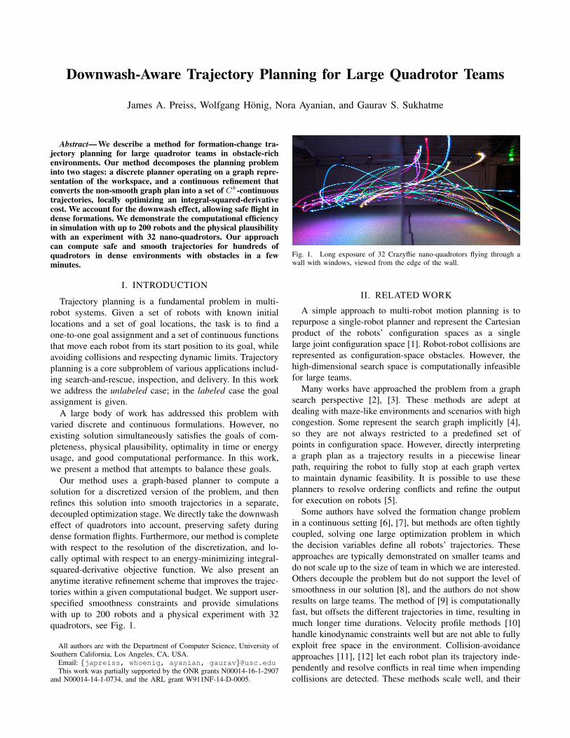
Rotorcraft generate a large, fast-moving volume of airunderneath their rotors called downwash. The downwashforce is large enough to cause a catastrophic loss of stabilitywhen one rotorcraft flies underneath another. We modeldownwash constraints by treating each robot as an axis-aligned ellipsoid of radii 0 < rx = ry rz , illustrated inFig. 2. Empirical data collected in [16], [17] support thismodel. The set of points representing a robot at positionq ∈ R3 is given by

E(q) = Ex+ q : ‖x‖2 ≤ 1 (1)

where E = diag(rx, ry, rz). The collision-avoidance con-straint between robots located at p, q ∈ R3 is given by

‖E−1(p− q)‖2 ≥ 2. (2)

Fig. 2. Axis-aligned ellipsoid model of robot volume. Tall height preventsdownwash interference between quadrotors.

B. Problem Statement

Consider a team of N robots in a bounded environmentcontaining convex obstacles O1 . . .ONobs

. Boundaries of theenvironment are defined by a convex polytope W . The freeconfiguration space for a single robot is thus given by

F = (W \ (⋃hOh)) E(0) (3)

where denotes the Minkowski difference.We are given a start position for each robot si ∈ F and

a set of goal positions G ⊂ F , |G| = N . The start and goalinputs must satisfy the collision constraint (2) for all robotpairs. We seek the following:• An assignment of each robot to a goal positiongφ(i) ∈ G, where φ is a permutation of 1 . . . N

• The total time duration T ∈ R>0 until the last robotreaches its goal

• For each robot ri, a trajectory f i : [0, T ] 7→ F wheref i(0) = si, f i(T ) = gφ(i), and f i must be continuousup to a user-specified parameter C:

dc

dtcf i(t) continuous for all c ∈ 1 . . . C. (4)

Additionally, we require that the collision-avoidanceconstraint (2) is satisfied at all times for all pairs ofrobots.

In the following, we present an efficient solution to thesubclass of problems where all si and gi are positions in anorthogonal grid and obstacles are cubes within that grid.

C. Overview

Our approach decomposes the formation change probleminto two steps: Discrete Planning and Continuous Refine-ment. Discrete planning solves the goal assignment problem(generating φ) and computes a timed sequence of waypointsfor each robot in a graph approximation of the environment.Continuous refinement uses the discrete plan as a startingpoint to compute a set of smooth trajectories satisfying user-supplied smoothness constraints.

We note that a major benefit of our method is its abilityto use different discrete planners. For example, it would bepossible to use a discrete planner for planning problemswhere the goal assignment is fixed a-priori, or where robotsare split into smaller groups.

IV. DISCRETE PLANNING STAGE

The discrete planning stage works with a grid discretiza-tion of the environment. We assume that the robots’ start andgoal locations are vertices of the underlying graph.

A. Overview

The discrete planning stage computes the goal assign-ment φ and a path pi for each robot composed of a sequenceof K + 1 (time, position) pairs:

pi = (t0, xi0), (t1, x

i1), . . . , (tK , x

iK) (5)

where 0 = t0 < t1 < · · · < tK = T , xik ∈ F , xi0 = si, andxiK = gφ(i). In between waypoints (tk, x

ik) and (tk+1, x

ik+1),

we assume that robot i travels on the line segment betweenxik and xik+1, but we do not make any assumptions aboutthe velocity profile of the robot along that path. We denotethis line segment by `ik.

We require that the discrete planner supplies a plan thatsatisfies the ellipsoid collision-avoidance constraint (2) for allpossible identical velocity profiles. We also require all robotsto share the same sequence of waypoint times t0 . . . tK .

In the following, we discuss one specific discrete plannerthat simultaneously computes the goal assignment φ andproduces waypoint sequences pi that minimize K. Thisplanner operates in a grid environment and assumes fixedtimesteps, i.e. tk+1 − tk is equal for all k. Furthermore, werequire the grid size to be greater than 2rx. A robot caneither move to an adjacent grid cell or stay at its currentlocation each step. At all timesteps, and during movements,the planner must ensure that the collision constraints arefulfilled. With fixed timesteps, the number of waypointsK corresponds to the time duration of the trajectory. Kis known as the makespan. Our planner minimizes K toproduce short trajectories.

B. Unlabeled Planner

We model unlabeled planning as a variant of the unla-beled Multi-Agent Path-Finding (MAPF) problem. We aregiven an undirected connected graph of the environmentGE = (VE , EE), where each vertex v ∈ VE corresponds toa location in F and each edge (u, v) ∈ EE denotes thatthere is a linear path in F connecting u and v. Obstacles areimplicitly modeled by not including a vertex in VE for eachcell that contains an obstacle. We assume that there exists avertex vis ∈ VE corresponding to each start location si and

that there exists a vertex vig ∈ VE for each goal location gi.At each discrete timestep, a robot can either wait at its currentvertex or traverse an edge. For the following formulation, weassume that the locations corresponding to the vertices arein a grid world and that z(·) and xy(·) map a vector to its zand x, y components, respectively. Our goal is to find pathspi, such that the following properties hold:

P1: Each robot starts at its start vertex: ∀i : xi0 = si.P2: Each robot ends at its goal vertex: ∀i : xiK = gφ(i).P3: At each timestep, each robot either stays at its current

position or traverses an edge: ∀k, ∀i: xik = xik+1 or∃ (u, v) ∈ EE s.t. u and v correspond to xik and xik+1.

P4: No robots occupy the same location at the same time(vertex collision): ∀k, ∀i 6= j: xik 6= xjk.

P5: No robots traverse the same edge in opposite directions(edge collision): ∀k, ∀i 6= j: xik 6= xjk+1 or xjk 6= xik+1.

P6: Robots obey downwash constraints when stationary(downwash vertex collision): ∀k, ∀i 6= j wherexy(xik) = xy(xjk): |z(xik)− z(xjk)| ≥ 2rz .

P7: Robots obey downwash constraints while traversing anedge (downwash edge collision): ∀k, ∀i 6= j wherexy(xik) = xy(xjk+1), xy(xjk) = xy(xik+1): |z(xik) −z(xjk+1)| ≥ 2rz or |z(xjk)− z(xik+1)| ≥ 2rz .

We consider a solution optimal if the makespan K isminimal. If only the first five properties are considered and Kis given, unlabeled MAPF can be solved in polynomial timeby reduction to a maximum-flow problem in a larger graph,derived from G, known as a time-expanded flow-graph [18].This graph, denoted by GF , contains O(K ·|VE |) vertices andis constructed such that a flow in GF represents a solutionto the MAPF instance. This maximum-flow problem canalso be expressed as an Integer Linear Program (ILP) whereeach edge is modeled as binary variable indicating its flowand the objective is to maximize the flow subject to flowconservation constraints [19]. An ILP formulation allows usto add additional constraints for P6 and P7.

We build the time-expanded flow-graph GF = (VF , EF )as intermediate step to formulate the ILP. Compared tothe existing detailed discussions [18], [19], [20], we addadditional annotations con : EF 7→ 2EF to some of the edgessuch that con(e) is the set of edges with which e is in conflictunder the downwash model. For each timestep k and vertexv ∈ VE we add two vertices uvk and wvk to VF and create anedge connecting them.

as1

b

cg1

(a) GE

uv1k

uv2k

wv1k

wv2k

(b) “Gadget” for flow-graph construction.

ua0

ub0

uc0

wa0

wb0

wc0

ua1

ub1

uc1

wa1

wb1

wc1

source

sink

(c) GF with K = 2.

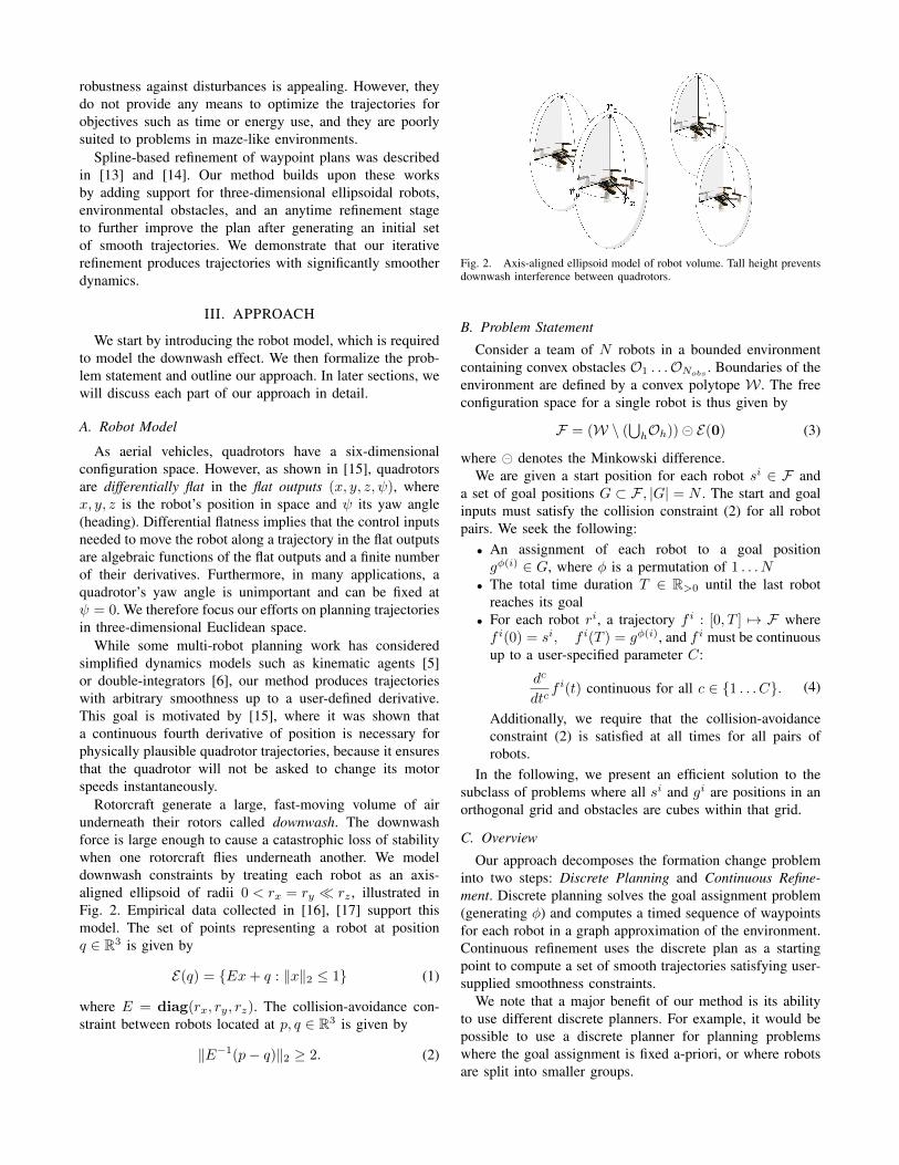
Fig. 3. Example flow-graph (Fig. 3(c)) for environment shown in Fig. 3(a) with a single robot. The construction uses a graph “gadget” (Fig. 3(b)) foreach edge in GE . The blue edges are annotated with downwash edge conflicts and the green edges are annotated with downwash vertex conflicts. Thebold arrows in Fig. 3(c) show the maximum flow through the network, which can be used to compute the robots’ paths.

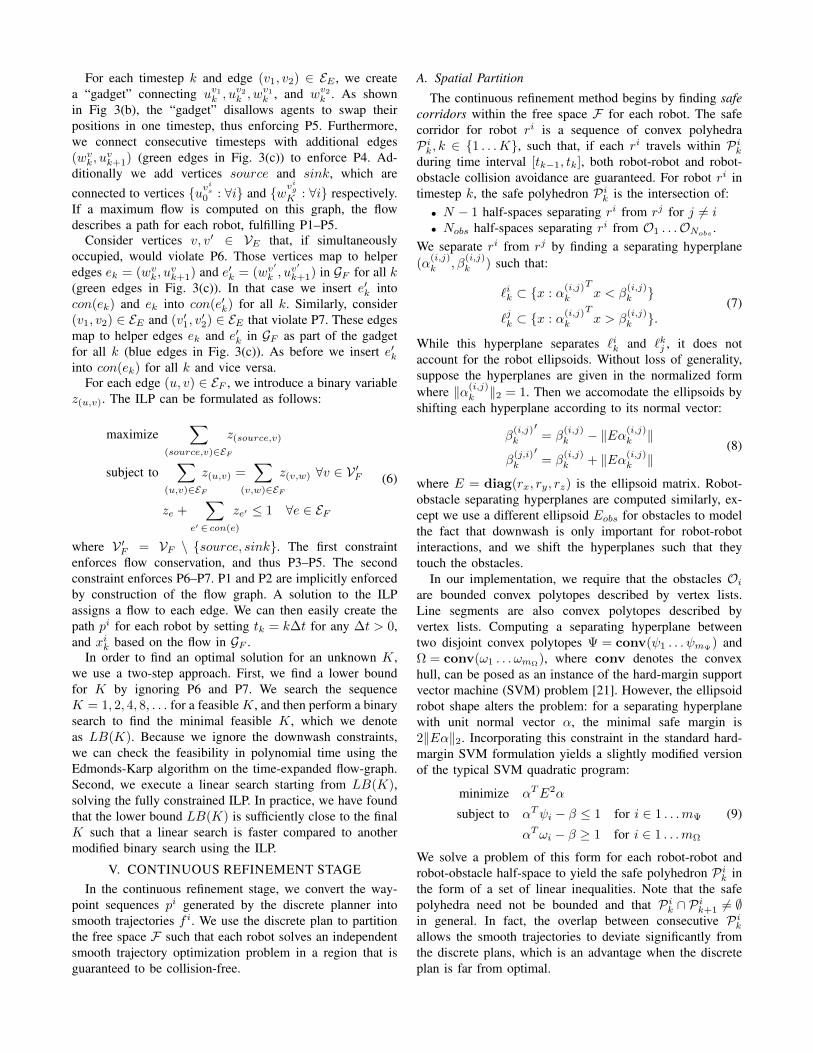
For each timestep k and edge (v1, v2) ∈ EE , we createa “gadget” connecting uv1

k , uv2

k , wv1

k , and wv2

k . As shownin Fig 3(b), the “gadget” disallows agents to swap theirpositions in one timestep, thus enforcing P5. Furthermore,we connect consecutive timesteps with additional edges(wvk, u

vk+1) (green edges in Fig. 3(c)) to enforce P4. Ad-

ditionally we add vertices source and sink, which areconnected to vertices uv

is

0 : ∀i and wvig

K : ∀i respectively.If a maximum flow is computed on this graph, the flowdescribes a path for each robot, fulfilling P1–P5.

Consider vertices v, v′ ∈ VE that, if simultaneouslyoccupied, would violate P6. Those vertices map to helperedges ek = (wvk, u

vk+1) and e′k = (wv

′

k , uv′

k+1) in GF for all k(green edges in Fig. 3(c)). In that case we insert e′k intocon(ek) and ek into con(e′k) for all k. Similarly, consider(v1, v2) ∈ EE and (v′1, v

′2) ∈ EE that violate P7. These edges

map to helper edges ek and e′k in GF as part of the gadgetfor all k (blue edges in Fig. 3(c)). As before we insert e′kinto con(ek) for all k and vice versa.

For each edge (u, v) ∈ EF , we introduce a binary variablez(u,v). The ILP can be formulated as follows:

maximize∑

(source,v)∈EF

z(source,v)

subject to∑

(u,v)∈EF

z(u,v) =∑

(v,w)∈EF

z(v,w) ∀v ∈ V ′F

ze +∑

e′ ∈ con(e)

ze′ ≤ 1 ∀e ∈ EF

(6)

where V ′F = VF \ source, sink. The first constraintenforces flow conservation, and thus P3–P5. The secondconstraint enforces P6–P7. P1 and P2 are implicitly enforcedby construction of the flow graph. A solution to the ILPassigns a flow to each edge. We can then easily create thepath pi for each robot by setting tk = k∆t for any ∆t > 0,and xik based on the flow in GF .

In order to find an optimal solution for an unknown K,we use a two-step approach. First, we find a lower boundfor K by ignoring P6 and P7. We search the sequenceK = 1, 2, 4, 8, . . . for a feasible K, and then perform a binarysearch to find the minimal feasible K, which we denoteas LB(K). Because we ignore the downwash constraints,we can check the feasibility in polynomial time using theEdmonds-Karp algorithm on the time-expanded flow-graph.Second, we execute a linear search starting from LB(K),solving the fully constrained ILP. In practice, we have foundthat the lower bound LB(K) is sufficiently close to the finalK such that a linear search is faster compared to anothermodified binary search using the ILP.

V. CONTINUOUS REFINEMENT STAGEIn the continuous refinement stage, we convert the way-

point sequences pi generated by the discrete planner intosmooth trajectories f i. We use the discrete plan to partitionthe free space F such that each robot solves an independentsmooth trajectory optimization problem in a region that isguaranteed to be collision-free.

A. Spatial Partition

The continuous refinement method begins by finding safecorridors within the free space F for each robot. The safecorridor for robot ri is a sequence of convex polyhedraPik, k ∈ 1 . . .K, such that, if each ri travels within Pikduring time interval [tk−1, tk], both robot-robot and robot-obstacle collision avoidance are guaranteed. For robot ri intimestep k, the safe polyhedron Pik is the intersection of:• N − 1 half-spaces separating ri from rj for j 6= i• Nobs half-spaces separating ri from O1 . . .ONobs

.We separate ri from rj by finding a separating hyperplane(α

(i,j)k , β

(i,j)k ) such that:

`ik ⊂ x : α(i,j)k

Tx < β

(i,j)k

`jk ⊂ x : α(i,j)k

Tx > β

(i,j)k .

(7)

While this hyperplane separates `ik and `kj , it does notaccount for the robot ellipsoids. Without loss of generality,suppose the hyperplanes are given in the normalized formwhere ‖α(i,j)

k ‖2 = 1. Then we accomodate the ellipsoids byshifting each hyperplane according to its normal vector:

β(i,j)k

′= β

(i,j)k − ‖Eα(i,j)

k ‖

β(j,i)k

′= β

(i,j)k + ‖Eα(i,j)

k ‖(8)

where E = diag(rx, ry, rz) is the ellipsoid matrix. Robot-obstacle separating hyperplanes are computed similarly, ex-cept we use a different ellipsoid Eobs for obstacles to modelthe fact that downwash is only important for robot-robotinteractions, and we shift the hyperplanes such that theytouch the obstacles.

In our implementation, we require that the obstacles Oiare bounded convex polytopes described by vertex lists.Line segments are also convex polytopes described byvertex lists. Computing a separating hyperplane betweentwo disjoint convex polytopes Ψ = conv(ψ1 . . . ψmΨ

) andΩ = conv(ω1 . . . ωmΩ

), where conv denotes the convexhull, can be posed as an instance of the hard-margin supportvector machine (SVM) problem [21]. However, the ellipsoidrobot shape alters the problem: for a separating hyperplanewith unit normal vector α, the minimal safe margin is2‖Eα‖2. Incorporating this constraint in the standard hard-margin SVM formulation yields a slightly modified versionof the typical SVM quadratic program:

minimize αTE2α

subject to αTψi − β ≤ 1 for i ∈ 1 . . .mΨ

αTωi − β ≥ 1 for i ∈ 1 . . .mΩ

(9)

We solve a problem of this form for each robot-robot androbot-obstacle half-space to yield the safe polyhedron Pik inthe form of a set of linear inequalities. Note that the safepolyhedra need not be bounded and that Pik ∩ Pik+1 6= ∅in general. In fact, the overlap between consecutive Pikallows the smooth trajectories to deviate significantly fromthe discrete plans, which is an advantage when the discreteplan is far from optimal.

B. Bezier Trajectory basis

After computing safe corridors, we plan a smooth trajec-tory f i(t) for each robot, contained within the robot’s safecorridor. We represent these trajectories as piecewise polyno-mials with one piece per time interval [tk, tk+1]. Piecewisepolynomials are widely used for trajectory planning: with anappropriate choice of degree and number of pieces, they canrepresent arbitrarily complex trajectories with an arbitrarynumber of continuous derivatives.

We denote the kth piece of robot i’s piecewise polynomialtrajectory as f ik. We wish to constrain f ik to lie within thesafe polyhedron Pik. However, when working in the standardmonomial basis, i.e. when the decision variables are the aiin the expression

p(t) = a0 + a1t+ a2t2 + · · ·+ aDt

D,

bounding the polynomial inside a convex polyhedron is nota convex constraint. Instead, we formulate trajectories asBezier curves. A degree-D Bezier curve is defined by asequence of D+ 1 control points yi ∈ R3 and a fixed set ofBernstein polynomials, such that

f(t) = b0,D(t)y0 + b1,D(t)y1 + · · ·+ bD,D(t)yD (10)

where each bi,D is a degree-D Bernstein polynomial withcoefficients1 given in [22]. The curve begins at y0 and endsat yD. In between, it does not pass through the interveningcontrol points, but rather is guaranteed to lie in the convexhull of all control points. Thus, when using Bezier controlpoints as decision variables instead of monomial coefficients,constraining the control points to lie inside a safe polyhedronguarantees that the resulting polynomial will lie inside thepolyhedron also. We define f i as a K-piece, degree-D Beziercurve and denote the dth control point of f ik as yik,d. Thedegree parameter D must be sufficiently high to ensurecontinuity at the user-defined continuity level C.

C. Optimization Problem

The set of Bezier curves that lie within a given safecorridor describes a family of feasible solutions to a singlerobot’s planning problem. We select an optimal trajectory byminimizing a weighted combination of the integrated squaredderivatives:

cost(f i) =

C∑c=1

γc

∫ T

0

∥∥∥∥ dcdtc f i(t)∥∥∥∥2

2

dt (11)

where the γc ≥ 0 are user-chosen weights on the derivatives.A typical choice in our experiments is to penalize accelera-tion and snap equally. As an input to the trajectory optimiza-tion stage, we require the user to supply an initial guess ofthe duration ∆t of each timestep, such that T = K∆t.

Our decision variable y consists of all control points forf i concatenated together:

y =[yi1,0

T. . . yi1,D

T, . . . , yiK,0

T. . . yiK,D

T]T

(12)

1 The canonical Bernstein polynomials are defined over the time interval[0, 1], but they are easily modified to span our desired time interval.

The objective function (11) is a quadratic function of y,which can be expressed in the form:

cost(f i) = yT (BTQB)y (13)

where B is a block-diagonal matrix transforming controlpoints into polynomial coefficients, and the formula for Q isgiven in [23]. The start and goal position constraints, as wellas the continuity constraints between successive polynomialpieces, can be expressed as linear equalities. Thus, we solvethe quadratic program:

minimize yT (BTQB)y

subject to yik,d ∈ Pik ∀ i, k, df i(0) = si, f i(T ) = gφ(i)

f i continuous up to derivative Cdc

dtcf i(t) = 0 ∀ c > 0, t ∈ 0, T

(14)

It is important to note that this quadratic program may notalways have a solution due to our conservative assumptionsregarding velocity profiles. In these cases, we fall back on asolution that follows the discrete plan exactly, coming to acomplete stop at corners. Details of this solution are givenin [13].

The corridor-constrained Bezier formulation presents onenotable shortcoming: for a given safe polyhedron Pik, thereexist degree-D polynomials that lie inside the polyhedronbut cannot be expressed as a Bezier curve with control pointsthat are contained within Pik. Empirical exploration of Beziercurves suggests that this problem is most significant when thedesired trajectory is near the faces of the polyhedron ratherthan the center. Further research is needed to characterizethis issue more precisely.

D. Iterative Refinement

Solving (14) for each robot converts the discrete plan intoa set of smooth trajectories that are locally optimal giventhe spatial decomposition. However, these trajectories arenot globally optimal. In our experiments, we found that thesmooth trajectories sometimes lie quite far away from theoriginal discrete plan. Motivated by this observation, weimplement an iterative refinement stage where we use thesmooth trajectories to define a new spatial decomposition,

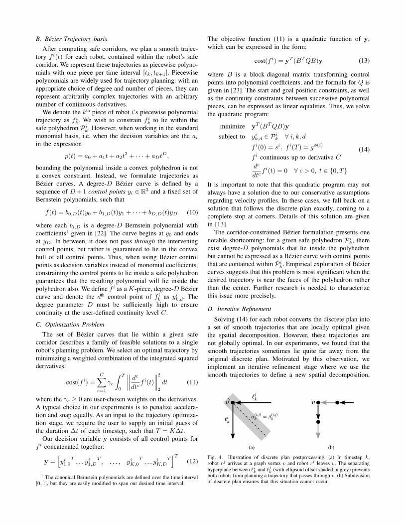
(a) (b)

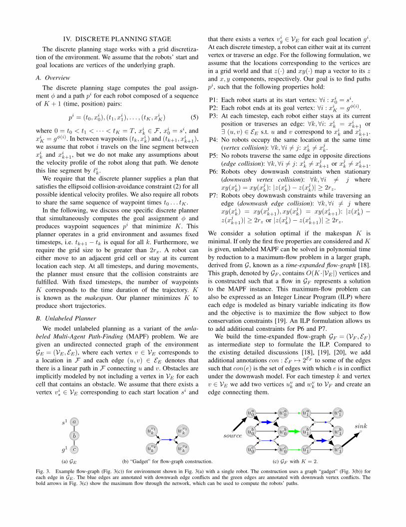
Fig. 4. Illustration of discrete plan postprocessing. (a) In timestep k,robot rj arrives at a graph vertex v and robot ri leaves v. The separatinghyperplane between `ik and `jk (with ellipsoid offset shaded in grey) preventsboth robots from planning a trajectory that passes through v. (b) Subdivisionof discrete plan ensures that this situation cannot occur.

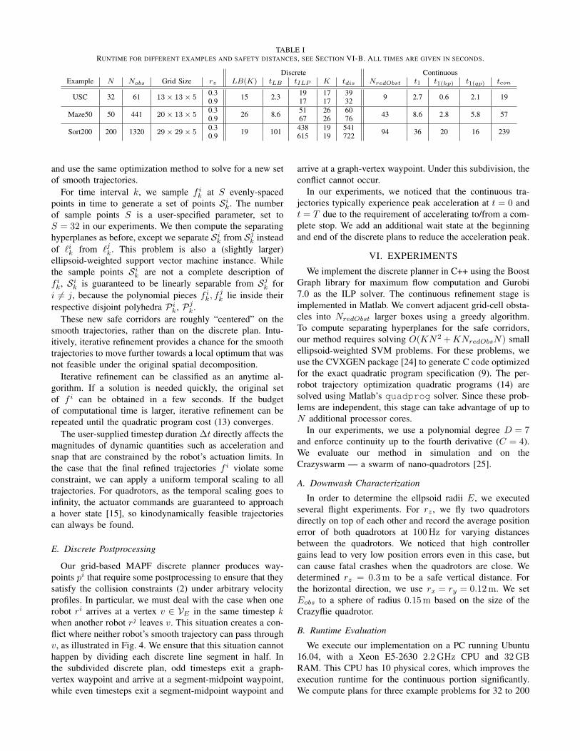
TABLE IRUNTIME FOR DIFFERENT EXAMPLES AND SAFETY DISTANCES, SEE SECTION VI-B. ALL TIMES ARE GIVEN IN SECONDS.

Discrete ContinuousExample N Nobs Grid Size rz LB(K) tLB tILP K tdis NredObst t1 t1(hp) t1(qp) tcon

USC 32 61 13× 13× 50.3 15 2.3 19 17 39 9 2.7 0.6 2.1 190.9 17 17 32

Maze50 50 441 20× 13× 50.3 26 8.6 51 26 60 43 8.6 2.8 5.8 570.9 67 26 76

Sort200 200 1320 29× 29× 50.3 19 101 438 19 541 94 36 20 16 2390.9 615 19 722

and use the same optimization method to solve for a new setof smooth trajectories.

For time interval k, we sample f ik at S evenly-spacedpoints in time to generate a set of points Sik. The numberof sample points S is a user-specified parameter, set toS = 32 in our experiments. We then compute the separatinghyperplanes as before, except we separate Sik from Sjk insteadof `ik from `jk. This problem is also a (slightly larger)ellipsoid-weighted support vector machine instance. Whilethe sample points Sik are not a complete description off ik, Sik is guaranteed to be linearly separable from Sjk fori 6= j, because the polynomial pieces f ik, f

jk lie inside their

respective disjoint polyhedra Pik, Pjk .These new safe corridors are roughly “centered” on the

smooth trajectories, rather than on the discrete plan. Intu-itively, iterative refinement provides a chance for the smoothtrajectories to move further towards a local optimum that wasnot feasible under the original spatial decomposition.

Iterative refinement can be classified as an anytime al-gorithm. If a solution is needed quickly, the original setof f i can be obtained in a few seconds. If the budgetof computational time is larger, iterative refinement can berepeated until the quadratic program cost (13) converges.

The user-supplied timestep duration ∆t directly affects themagnitudes of dynamic quantities such as acceleration andsnap that are constrained by the robot’s actuation limits. Inthe case that the final refined trajectories f i violate someconstraint, we can apply a uniform temporal scaling to alltrajectories. For quadrotors, as the temporal scaling goes toinfinity, the actuator commands are guaranteed to approacha hover state [15], so kinodynamically feasible trajectoriescan always be found.

E. Discrete Postprocessing

Our grid-based MAPF discrete planner produces way-points pi that require some postprocessing to ensure that theysatisfy the collision constraints (2) under arbitrary velocityprofiles. In particular, we must deal with the case when onerobot ri arrives at a vertex v ∈ VE in the same timestep kwhen another robot rj leaves v. This situation creates a con-flict where neither robot’s smooth trajectory can pass throughv, as illustrated in Fig. 4. We ensure that this situation cannothappen by dividing each discrete line segment in half. Inthe subdivided discrete plan, odd timesteps exit a graph-vertex waypoint and arrive at a segment-midpoint waypoint,while even timesteps exit a segment-midpoint waypoint and

arrive at a graph-vertex waypoint. Under this subdivision, theconflict cannot occur.

In our experiments, we noticed that the continuous tra-jectories typically experience peak acceleration at t = 0 andt = T due to the requirement of accelerating to/from a com-plete stop. We add an additional wait state at the beginningand end of the discrete plans to reduce the acceleration peak.

VI. EXPERIMENTS

We implement the discrete planner in C++ using the BoostGraph library for maximum flow computation and Gurobi7.0 as the ILP solver. The continuous refinement stage isimplemented in Matlab. We convert adjacent grid-cell obsta-cles into NredObst larger boxes using a greedy algorithm.To compute separating hyperplanes for the safe corridors,our method requires solving O(KN2 +KNredObsN) smallellipsoid-weighted SVM problems. For these problems, weuse the CVXGEN package [24] to generate C code optimizedfor the exact quadratic program specification (9). The per-robot trajectory optimization quadratic programs (14) aresolved using Matlab’s quadprog solver. Since these prob-lems are independent, this stage can take advantage of up toN additional processor cores.

In our experiments, we use a polynomial degree D = 7and enforce continuity up to the fourth derivative (C = 4).We evaluate our method in simulation and on theCrazyswarm — a swarm of nano-quadrotors [25].

A. Downwash Characterization

In order to determine the ellpsoid radii E, we executedseveral flight experiments. For rz , we fly two quadrotorsdirectly on top of each other and record the average positionerror of both quadrotors at 100 Hz for varying distancesbetween the quadrotors. We noticed that high controllergains lead to very low position errors even in this case, butcan cause fatal crashes when the quadrotors are close. Wedetermined rz = 0.3 m to be a safe vertical distance. Forthe horizontal direction, we use rx = ry = 0.12 m. We setEobs to a sphere of radius 0.15 m based on the size of theCrazyflie quadrotor.

B. Runtime Evaluation

We execute our implementation on a PC running Ubuntu16.04, with a Xeon E5-2630 2.2 GHz CPU and 32 GBRAM. This CPU has 10 physical cores, which improves theexecution runtime for the continuous portion significantly.We compute plans for three example problems for 32 to 200

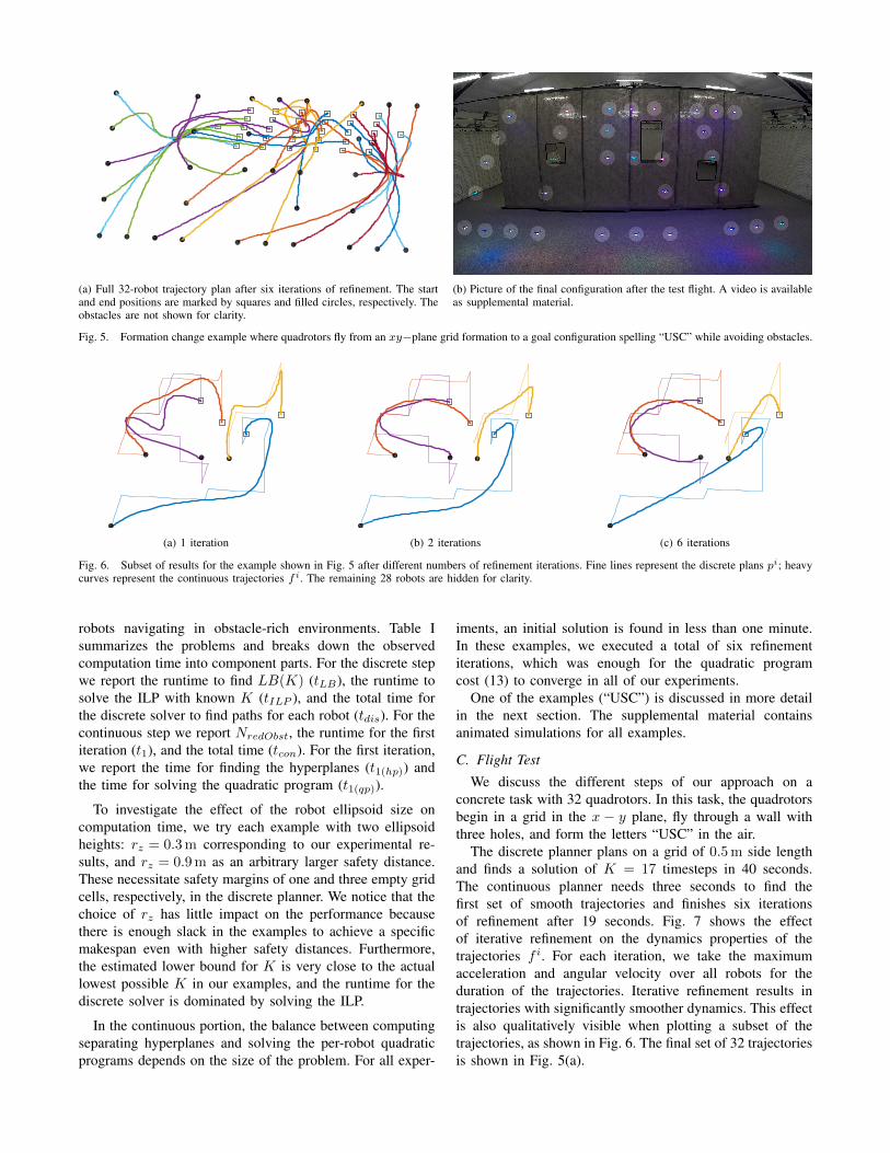
(a) Full 32-robot trajectory plan after six iterations of refinement. The startand end positions are marked by squares and filled circles, respectively. Theobstacles are not shown for clarity.

(b) Picture of the final configuration after the test flight. A video is availableas supplemental material.

Fig. 5. Formation change example where quadrotors fly from an xy−plane grid formation to a goal configuration spelling “USC” while avoiding obstacles.

(a) 1 iteration (b) 2 iterations (c) 6 iterations

Fig. 6. Subset of results for the example shown in Fig. 5 after different numbers of refinement iterations. Fine lines represent the discrete plans pi; heavycurves represent the continuous trajectories f i. The remaining 28 robots are hidden for clarity.

robots navigating in obstacle-rich environments. Table Isummarizes the problems and breaks down the observedcomputation time into component parts. For the discrete stepwe report the runtime to find LB(K) (tLB), the runtime tosolve the ILP with known K (tILP ), and the total time forthe discrete solver to find paths for each robot (tdis). For thecontinuous step we report NredObst, the runtime for the firstiteration (t1), and the total time (tcon). For the first iteration,we report the time for finding the hyperplanes (t1(hp)) andthe time for solving the quadratic program (t1(qp)).

To investigate the effect of the robot ellipsoid size oncomputation time, we try each example with two ellipsoidheights: rz = 0.3 m corresponding to our experimental re-sults, and rz = 0.9 m as an arbitrary larger safety distance.These necessitate safety margins of one and three empty gridcells, respectively, in the discrete planner. We notice that thechoice of rz has little impact on the performance becausethere is enough slack in the examples to achieve a specificmakespan even with higher safety distances. Furthermore,the estimated lower bound for K is very close to the actuallowest possible K in our examples, and the runtime for thediscrete solver is dominated by solving the ILP.

In the continuous portion, the balance between computingseparating hyperplanes and solving the per-robot quadraticprograms depends on the size of the problem. For all exper-

iments, an initial solution is found in less than one minute.In these examples, we executed a total of six refinementiterations, which was enough for the quadratic programcost (13) to converge in all of our experiments.

One of the examples (“USC”) is discussed in more detailin the next section. The supplemental material containsanimated simulations for all examples.

C. Flight Test

We discuss the different steps of our approach on aconcrete task with 32 quadrotors. In this task, the quadrotorsbegin in a grid in the x − y plane, fly through a wall withthree holes, and form the letters “USC” in the air.

The discrete planner plans on a grid of 0.5 m side lengthand finds a solution of K = 17 timesteps in 40 seconds.The continuous planner needs three seconds to find thefirst set of smooth trajectories and finishes six iterationsof refinement after 19 seconds. Fig. 7 shows the effectof iterative refinement on the dynamics properties of thetrajectories f i. For each iteration, we take the maximumacceleration and angular velocity over all robots for theduration of the trajectories. Iterative refinement results intrajectories with significantly smoother dynamics. This effectis also qualitatively visible when plotting a subset of thetrajectories, as shown in Fig. 6. The final set of 32 trajectoriesis shown in Fig. 5(a).

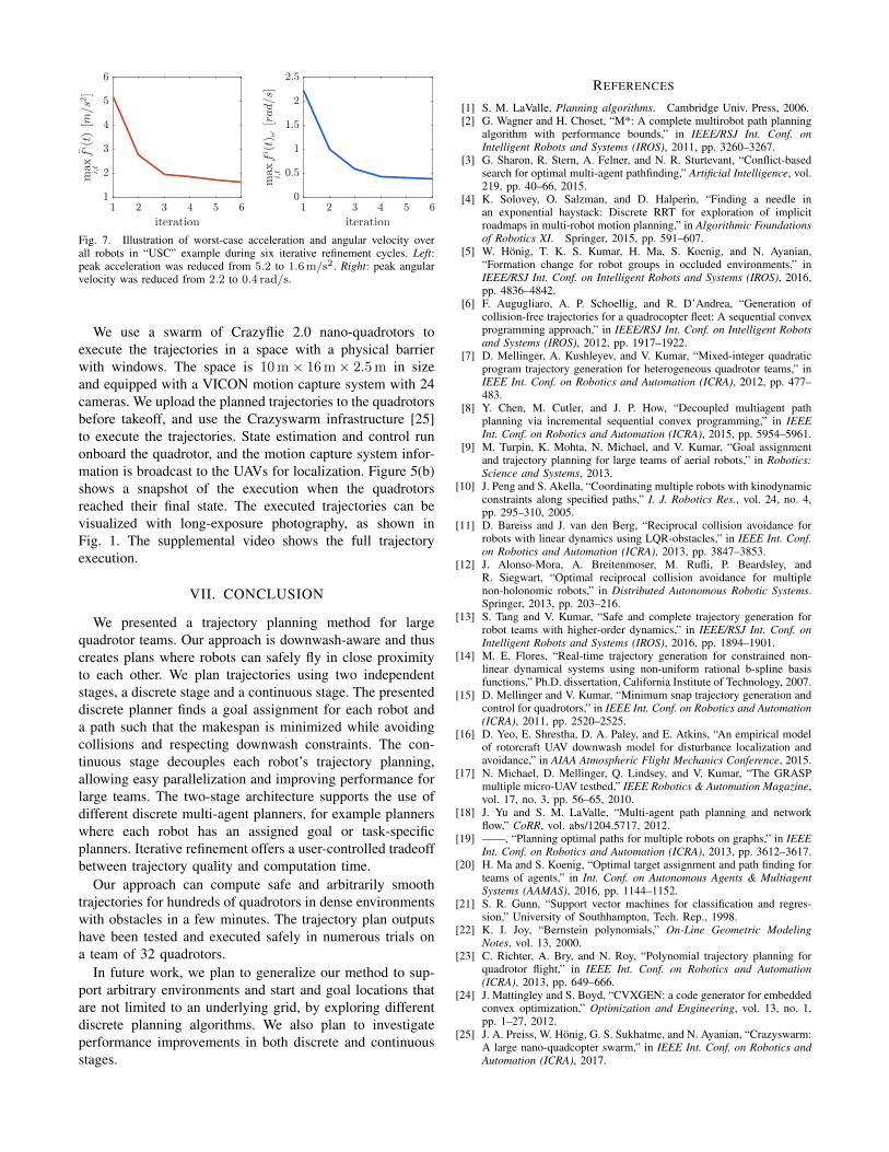
Fig. 7. Illustration of worst-case acceleration and angular velocity overall robots in “USC” example during six iterative refinement cycles. Left:peak acceleration was reduced from 5.2 to 1.6m/s2. Right: peak angularvelocity was reduced from 2.2 to 0.4 rad/s.

We use a swarm of Crazyflie 2.0 nano-quadrotors toexecute the trajectories in a space with a physical barrierwith windows. The space is 10 m× 16 m× 2.5 m in sizeand equipped with a VICON motion capture system with 24cameras. We upload the planned trajectories to the quadrotorsbefore takeoff, and use the Crazyswarm infrastructure [25]to execute the trajectories. State estimation and control runonboard the quadrotor, and the motion capture system infor-mation is broadcast to the UAVs for localization. Figure 5(b)shows a snapshot of the execution when the quadrotorsreached their final state. The executed trajectories can bevisualized with long-exposure photography, as shown inFig. 1. The supplemental video shows the full trajectoryexecution.

VII. CONCLUSION

We presented a trajectory planning method for largequadrotor teams. Our approach is downwash-aware and thuscreates plans where robots can safely fly in close proximityto each other. We plan trajectories using two independentstages, a discrete stage and a continuous stage. The presenteddiscrete planner finds a goal assignment for each robot anda path such that the makespan is minimized while avoidingcollisions and respecting downwash constraints. The con-tinuous stage decouples each robot’s trajectory planning,allowing easy parallelization and improving performance forlarge teams. The two-stage architecture supports the use ofdifferent discrete multi-agent planners, for example plannerswhere each robot has an assigned goal or task-specificplanners. Iterative refinement offers a user-controlled tradeoffbetween trajectory quality and computation time.

Our approach can compute safe and arbitrarily smoothtrajectories for hundreds of quadrotors in dense environmentswith obstacles in a few minutes. The trajectory plan outputshave been tested and executed safely in numerous trials ona team of 32 quadrotors.

In future work, we plan to generalize our method to sup-port arbitrary environments and start and goal locations thatare not limited to an underlying grid, by exploring differentdiscrete planning algorithms. We also plan to investigateperformance improvements in both discrete and continuousstages.

REFERENCES

[1] S. M. LaValle, Planning algorithms. Cambridge Univ. Press, 2006.[2] G. Wagner and H. Choset, “M*: A complete multirobot path planning

algorithm with performance bounds,” in IEEE/RSJ Int. Conf. onIntelligent Robots and Systems (IROS), 2011, pp. 3260–3267.

[3] G. Sharon, R. Stern, A. Felner, and N. R. Sturtevant, “Conflict-basedsearch for optimal multi-agent pathfinding,” Artificial Intelligence, vol.219, pp. 40–66, 2015.

[4] K. Solovey, O. Salzman, and D. Halperin, “Finding a needle inan exponential haystack: Discrete RRT for exploration of implicitroadmaps in multi-robot motion planning,” in Algorithmic Foundationsof Robotics XI. Springer, 2015, pp. 591–607.

[5] W. Honig, T. K. S. Kumar, H. Ma, S. Koenig, and N. Ayanian,“Formation change for robot groups in occluded environments,” inIEEE/RSJ Int. Conf. on Intelligent Robots and Systems (IROS), 2016,pp. 4836–4842.

[6] F. Augugliaro, A. P. Schoellig, and R. D’Andrea, “Generation ofcollision-free trajectories for a quadrocopter fleet: A sequential convexprogramming approach,” in IEEE/RSJ Int. Conf. on Intelligent Robotsand Systems (IROS), 2012, pp. 1917–1922.

[7] D. Mellinger, A. Kushleyev, and V. Kumar, “Mixed-integer quadraticprogram trajectory generation for heterogeneous quadrotor teams,” inIEEE Int. Conf. on Robotics and Automation (ICRA), 2012, pp. 477–483.

[8] Y. Chen, M. Cutler, and J. P. How, “Decoupled multiagent pathplanning via incremental sequential convex programming,” in IEEEInt. Conf. on Robotics and Automation (ICRA), 2015, pp. 5954–5961.

[9] M. Turpin, K. Mohta, N. Michael, and V. Kumar, “Goal assignmentand trajectory planning for large teams of aerial robots,” in Robotics:Science and Systems, 2013.

[10] J. Peng and S. Akella, “Coordinating multiple robots with kinodynamicconstraints along specified paths,” I. J. Robotics Res., vol. 24, no. 4,pp. 295–310, 2005.

[11] D. Bareiss and J. van den Berg, “Reciprocal collision avoidance forrobots with linear dynamics using LQR-obstacles,” in IEEE Int. Conf.on Robotics and Automation (ICRA), 2013, pp. 3847–3853.

[12] J. Alonso-Mora, A. Breitenmoser, M. Rufli, P. Beardsley, andR. Siegwart, “Optimal reciprocal collision avoidance for multiplenon-holonomic robots,” in Distributed Autonomous Robotic Systems.Springer, 2013, pp. 203–216.

[13] S. Tang and V. Kumar, “Safe and complete trajectory generation forrobot teams with higher-order dynamics,” in IEEE/RSJ Int. Conf. onIntelligent Robots and Systems (IROS), 2016, pp. 1894–1901.

[14] M. E. Flores, “Real-time trajectory generation for constrained non-linear dynamical systems using non-uniform rational b-spline basisfunctions,” Ph.D. dissertation, California Institute of Technology, 2007.

[15] D. Mellinger and V. Kumar, “Minimum snap trajectory generation andcontrol for quadrotors,” in IEEE Int. Conf. on Robotics and Automation(ICRA), 2011, pp. 2520–2525.

[16] D. Yeo, E. Shrestha, D. A. Paley, and E. Atkins, “An empirical modelof rotorcraft UAV downwash model for disturbance localization andavoidance,” in AIAA Atmospheric Flight Mechanics Conference, 2015.

[17] N. Michael, D. Mellinger, Q. Lindsey, and V. Kumar, “The GRASPmultiple micro-UAV testbed,” IEEE Robotics & Automation Magazine,vol. 17, no. 3, pp. 56–65, 2010.

[18] J. Yu and S. M. LaValle, “Multi-agent path planning and networkflow,” CoRR, vol. abs/1204.5717, 2012.

[19] ——, “Planning optimal paths for multiple robots on graphs,” in IEEEInt. Conf. on Robotics and Automation (ICRA), 2013, pp. 3612–3617.

[20] H. Ma and S. Koenig, “Optimal target assignment and path finding forteams of agents,” in Int. Conf. on Autonomous Agents & MultiagentSystems (AAMAS), 2016, pp. 1144–1152.

[21] S. R. Gunn, “Support vector machines for classification and regres-sion,” University of Southhampton, Tech. Rep., 1998.

[22] K. I. Joy, “Bernstein polynomials,” On-Line Geometric ModelingNotes, vol. 13, 2000.

[23] C. Richter, A. Bry, and N. Roy, “Polynomial trajectory planning forquadrotor flight,” in IEEE Int. Conf. on Robotics and Automation(ICRA), 2013, pp. 649–666.

[24] J. Mattingley and S. Boyd, “CVXGEN: a code generator for embeddedconvex optimization,” Optimization and Engineering, vol. 13, no. 1,pp. 1–27, 2012.

[25] J. A. Preiss, W. Honig, G. S. Sukhatme, and N. Ayanian, “Crazyswarm:A large nano-quadcopter swarm,” in IEEE Int. Conf. on Robotics andAutomation (ICRA), 2017.