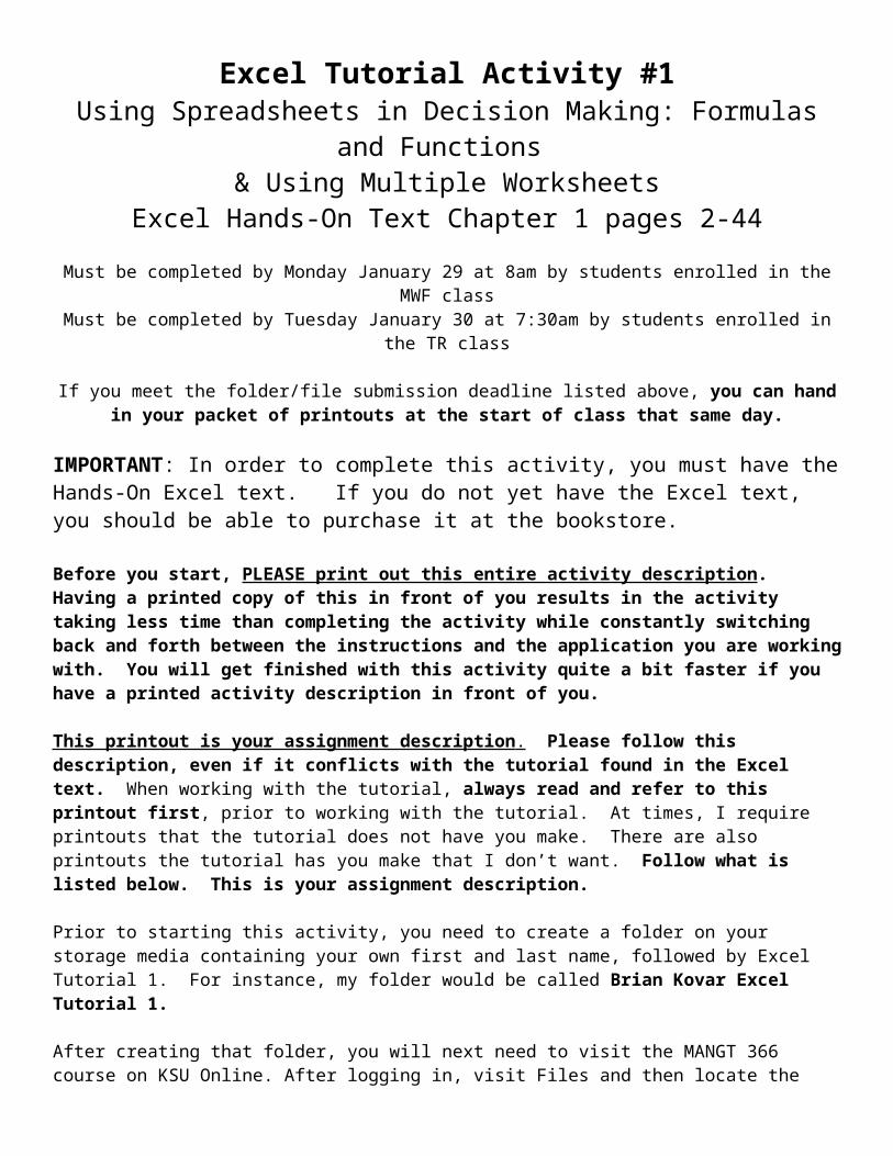
Excel Tutorial Activity #1Using Spreadsheets in Decision Making: Formulas and Functions

& Using Multiple WorksheetsExcel Hands-On Text Chapter 1 pages 2-44

Must be completed by Monday January 29 at 8am by students enrolled in the MWF classMust be completed by Tuesday January 30 at 7:30am by students enrolled in the TR class

If you meet the folder/file submission deadline listed above, you can hand in your packet of printouts at the start of class that same day.

IMPORTANT: In order to complete this activity, you must have the Hands-On Excel text. If you do not yet have the Excel text, you should be able to purchase it at the bookstore.

Before you start, PLEASE print out this entire activity description. Having a printed copy of this in front of you results in the activity taking less time than completing the activity while constantly switching back and forth between the instructions and the application you are working with. You will get finished with this activity quite a bit faster if you have a printed activity description in front of you.

This printout is your assignment description . Please follow this description, even if it conflicts with the tutorial found in the Excel text. When working with the tutorial, always read and refer to this printout first, prior to working with the tutorial. At times, I require printouts that the tutorial does not have you make. There are also printouts the tutorial has you make that I don’t want. Follow what is listed below. This is your assignment description.

Prior to starting this activity, you need to create a folder on your storage media containing your own first and last name, followed by Excel Tutorial 1. For instance, my folder would be called Brian Kovar Excel Tutorial 1.

After creating that folder, you will next need to visit the MANGT 366 course on KSU Online. After logging in, visit Files and then locate the Excel Tutorial Activity #1 folder. This folder contains Excel files to download for the first Excel tutorial activity. Download ALL OF THE FILES that you see into the folder that you just created. If you create any files from scratch as part of this activity, you will also need to save them into your named folder.

IMPORTANT: PLEASE READ: If a tutorial talks about getting files from some sort of folder or storage location, you will need to visit the folder that you just created/added to your storage media in the prior paragraph. All files that you don’t create yourself are already in that folder. When one of the tutorials tells you to save a file under a certain name, use the name required in the assignment description that you are currently reading (rather than the name found in the tutorial text).

SPECIAL NOTE: PLEASE READAll currency/dollar values found in this project must contain the $ symbol and be formatted using “Currency Style”. Please use the “true” currency style, rather than the $ button. Although the button is labeled as “$”, it is really Accounting Style. You want to use the true currency style, which results in a $ sign right next to the number, such as $45

Tutorial Excel activity #1 is composed of the following components:

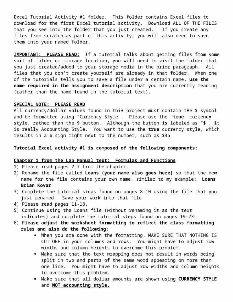
Chapter 1 from the Lab Manual text: Formulas and Functions1) Please read pages 2-7 from the chapter.2) Rename the file called Loans (your name also goes here) so that the new name for the file contains your

own name, similar to my example: Loans Brian Kovar 3) Complete the tutorial steps found on pages 8-10 using the file that you just renamed. Save your work into

that file.4) Please read pages 11-18.5) Continue using the Loans file (without renaming it as the text indicates) and complete the tutorial steps found

on pages 19-23.6) Please adjust the worksheet formatting to reflect the class formatting rules and also do the following:

When you are done with the formatting, MAKE SURE THAT NOTHING IS CUT OFF in your columns and rows. You might have to adjust row widths and column heights to overcome this problem.

Make sure that the text wrapping does not result in words being split in two and parts of the same word appearing on more than one line. You might have to adjust row widths and column heights to overcome this problem.

Make sure that all dollar amounts are shown using CURRENCY STYLE and NOT accounting style.

For neatness and professionalism, make sure that the labels in row 7 are centered. Make sure that the labels in row #7 are over the data that they describe. If you find that a label

has nothing underneath it, you will need to adjust the column width accordingly. Use Print Preview and go into the Page Setup/Scaling options (see pages 57 and 62 in your lab

manual). Make sure that1. Everything fits on one page. (scaling option). 2. The labels are DIRECTLY over the numbers that they describe.3. That the GRIDLINES DO NOT DISPLAY when the printout is made, and that the

column and row headings DO NOT DISPLAY either. In the workplace, it is considered very unprofessional to display spreadsheet gridlines, column headings and row headings when printing spreadsheets. DON’T PRINT THOSE THINGS.

Use the Page Setup feature to create a custom footer. The custom footer should be located in the center section of the worksheet. The first line of the custom footer should automatically display the worksheet name (there is a footer option button that does this). Immediately below this, the second line of the custom footer should display your first and last name (you will have to type this in on the second line of the custom footer)

8) Save your work and Hand in the following: A printout of the Details spreadsheet. A printout of the formulas created in the Details spreadsheet (Formulas tab, Show Formulas

option)9) Please read pages 24-31.10) Switch to the worksheet called Payment Info. 11) Begin with step #1B on page 32 and complete the tutorial steps as written until you complete the last

tutorial step on page 36.12) Make sure that all of your money amounts display using the currency style, rather than the

accounting style. 13) Make sure that you are following all of the class formatting rules in regards to the content of this worksheet.

In addition, please do the following: When you are done with the formatting, MAKE SURE THAT NOTHING IS CUT OFF in your

columns and rows. You might have to adjust row widths and column heights to overcome this problem.

Make sure that the text wrapping does not result in words being split in two and parts of the same word appearing on more than one line. You might have to adjust row widths and column heights to overcome this problem.

For neatness and professionalism, make sure that the labels in row 8 are centered. Make sure that the labels in row #8 are over the data that they describe. If you find that a label

has nothing underneath it, you will need to adjust the column width accordingly. Use Print Preview and go into the Page Setup options (see prior steps above where you did

this). Make sure that everything fits on one page, that the GRIDLINES DO NOT DISPLAY when the printout is made, and that the column and row headings DO NOT DISPLAY either. In the workplace, it is considered very unprofessional to display spreadsheet gridlines, column headings and row headings when printing spreadsheets. DON’T PRINT THOSE THINGS.

Use the Page Setup feature to create a custom footer. The custom footer should be located in the center section of the worksheet. The first line of the custom footer should automatically display the worksheet name (there is a footer option button that does this). Immediately below this, the second line of the custom footer should display your first and last name (you will have to type this in on the second line of the custom footer)

14) Hand in the following: A printout of the Payment Info spreadsheet. A printout of the formulas created in the Payment Info (Formulas tab, Show Formulas option)

15) Save your work. Close down this file.

Working With Multiple Worksheets)This next part of the tutorial activity deals with files containing multiple worksheets of related data. You can group worksheets so that you can perform one operation to several sheets at the same time (applying common formats to all sheets or creating formulas that do the same thing on different sheets). You can also create 3-D formulas that perform calculations using data on more than one sheet.

1) Open the file MultipleSheet (your name also goes here) and rename the file so that the new file name contains your last name, using the following example as a guide (MultipleSheet Kovar).

2) Click the Qtr1 worksheet tab, and then click each worksheet tab to see the differences. You should see that each worksheet appears different.

3) Click the Qtr1 worksheet tab, press and hold the Shift key, and then click on the Yearly Totals worksheet tab. You should now have grouped all of the worksheets together. Whatever you do to one sheet now happens on all of the grouped sheets. The title bar displays [Group] after the file name.

4) Click cell A1 in the Qtr1 worksheet to select it, click Fill in the Editing group on the Home tab, and then select Across Worksheets. When the Fill Across Worksheets dialog box opens, select All (indicating that you want to fill the content and the formatting) and then OK.

5) Right-click the Yearly Totals worksheet tab, and then select Ungroup Sheets. Please check all sheets to make sure that Heartland Department Store appears across the top of all sheets (in cell A1).

6) Return to the Qtr1. Copy the range A2:A9 using the Copy button.

7) Click the Qtr2 worksheet tab, press and hold the Shift key, and then click on the Yearly Totals worksheet tab. You have once again created a worksheet group. Click in cell A2 and click Paste. Next, widen out column A so that none of the words are cut off. These two actions (pasting and widening out the columns) is happening on all sheets in the worksheet group.

8) Click the Qtr1 worksheet tab to ungroup the sheets and then verify that you did take those actions on all sheets that made up the worksheet group.

9) Next, create a worksheet group comprised for the four quarterly sheets and do the following: Type Dept. Totals in cell E2. Use Format Painter to give cell E2 the same formats as used in cell D2. Widen out column E so that

nothing is cut off. Select the range E3:E9 and click the AutoSum button. Type Monthly Totals in cell A10. Use Format Painter to give cell A10 the same formats as used in cell

A2. Click the Increase Indent button once in cell A10. Select the range B10:E10 and click the AutoSum button. Apply the Currency Number Format to the range of B3:E3 and the range of B10:E10. Widen out any

columns that display #### Select the range of B4:E9. Right-click, select Format Cells, select Number, use the Number Format

and format the numbers to display two decimal places and use the 1000 Separator. Select the range B9:E9 Apply the Underline format to this range. Select the range B10:E10. Click the Underline Arrow in the font group and then select the Double

Underline option.

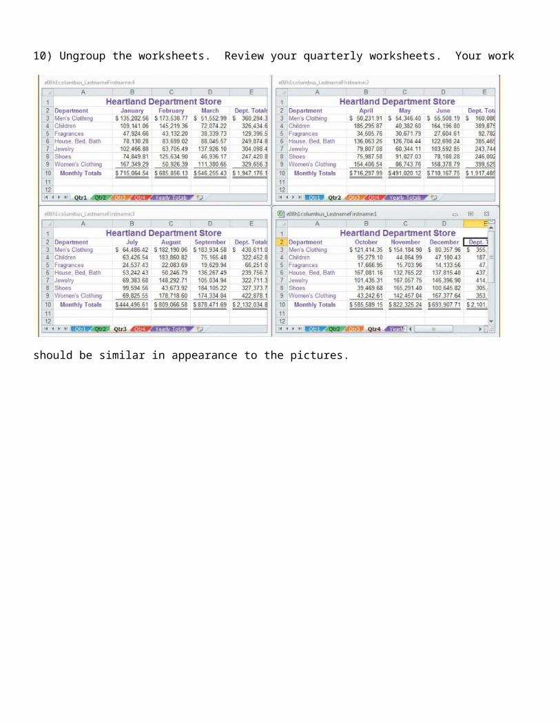
10) Ungroup the worksheets. Review your quarterly worksheets. Your work should be similar in appearance to the pictures.

11) Go to the Yearly Totals worksheet. Type in the following: Qtr1 in cell B2 Qtr2 in cell C2 Qtr3 in cell D2 Qtr4 in cell E2 Dept. Totals in cell F2

12) Format the range of B2:F2 so that those cells are purple, bold and centered. Widen out column F so that nothing is cut off.

The Yearly Totals worksheet is a summary worksheet that pulls data from the quarterly worksheets.

13) Click in cell B3 on the Yearly Totals worksheet. Do the following: Type an equals sign = Click on the Qtr1 worksheet tab Click cell E3 Press enter

You have now created a formula that pulls data from one sheet and places it on another sheet. Please look at the formula in the formula bar.

14) Do the following: Click in cell C3 and create a similar formula for quarter 2 Click in cell D3 and create a similar formula for quarter 3 Click in cell E3 and create a similar formula for quarter 4

15) When finished, copy the formulas in B3, C3,D3, E3 down so that all department categories display quarterly data.

16) Summarize the department to find the Department Totals

17) Cell A10 should display the label Quarterly Totals. It should display in purple font, bold and idented.

18) Summarize each quarter to find the quarterly totals.

19) Underline the Women’s Clothing numbers.Double underline the Quarterly Totals numbers

20) Make sure that your work matches the picture (in all aspects).

21) Create a worksheet group that includes all five sheets. Do the following to the group: Format the worksheets so that each will fit on 1 page and print in the landscape orientation Create a custom footer that will appear on all sheets. The custom footer should be centered and contain

the name of the worksheet, followed by your own name on the next line.

22) Save your work23) Print all 5 worksheets in the Multiple Sheets file (each on their own sheet of paper)24) Display the formulas on the Yearly Totals worksheet. Print those formulas

25) Proofread your printouts. Make sure that they are all formatted correctly and that the required footers display on each page. Sometimes, working with groups is tricky and something might not happen the way you think it should.

26) When you are happy with your work, save your work one last time and then close Excel.

HANDING IN THE ACTIVITY1) Submit ALL OF THE FILES THAT YOU WORKED WITH on this assignment to the KSU Online Canvas assignment submission location. You will submit two Excel files.

2) Please assemble your packet of printouts. The printouts should be arranged in the following order: A cover page containing the usual required information (which can also be found in the syllabus). The printout with the footer of Details The formulas for the Details printout The printout with the footer of Payment Info The formulas for the Payment Info printout The printout with the footer Qtr1. The printout with the footer Qtr2 The printout with the footer Qtr3 The printout with the footer Qtr4 The printout with the footer Yearly Totals The formulas for the Yearly Totals printout

IN ORDER TO BE CONSIDERED FOR FULL CREDIT, YOUR PRINTOUTS MUST BE IN THE REQUIRED SUBMISSION ORDER. Deductions will be taken for printouts that are not in the proper order.

FOLDER/FILE SUBMISSION TO THE APPROPRIATE KSU Canvas submission location, as well as submission of required printouts, MUST BE COMPLETED BY THE DATE AND TIME LISTED ABOVE (at the top of this activity description) .