Embed Size (px)
Citation preview
PRE-PROCESSING AND ANALYSIS
OF HIGH-DIMENSIONAL PLANT
METABOLOMICS DATA
Aikaterini KALOGEROPOULOU
May 2011
A thesis submitted in partial fulfilment of requirements for the degree of Master of
Philosophy of the University of East Anglia, Norwich, England.
Supported by the John Innes Centre and the Institute of Food Research
Norwich Research Park, Colney Lane, Norwich NR4 7U
© This copy of the thesis is supplied on condition that anyone who consults it is
understood to recognise that its copyright rests with the author and that no quotation
from the thesis, nor any information derived therefrom, may be published without
the author’s prior written consent.
1
CONTENTS
Acknowledgements……………………………………………......………………...5
Abstract………………………………………………………..…………………….6
Chapter 1: INTRODUCTION
1.1 Introduction to metabolomics……………………………………………...9
1.2 Analytical approaches………………………………………………………9
1.3 Data handling………………………………………………………………10
1.3.1 Data pre-processing………………………………………………..12
1.3.2 Data pre-treatment………………………………………………...12
1.3.3 Data analysis……...………………………………………………..13
1.3.4 Metabolite annotation……………………………………………..14
1.4 Applications of metabolomics in plant research…………………..……..15
1.4.1 Functional genomics………………………………..……………...15
1.4.2 Mutant analysis…………………………………………..………...15
1.5 Further challenges in plant metabolomics…………………….………....16
Chapter 2: METABOLOMIC TECHNOLOGIES
2.1 The extraction method…………………………………………..………...19
2.2 Mass Spectrometry……………………………………………..………….19
2.2.1 Ion sources…………………………………………..……………...22
2.2.1.1 Electron ionization…………………………………...…………….22
2.2.1.2 Electrospray ionization……………………………..……..24
2.2.2 Mass analyzers………………………………………………..…....24
2.2.2.1 The quadrupole………………………………..…………...26
2.2.2.2 Ion trap……………………………………………..……....26
2.2.3 Detectors………………………………………………………..…..26
2.2.4 Important MS parameters………………………………………...26
2.3 MS-chromatography coupling…………………………………….….…..27
2.3.1 Gas Chromatography………………………………….……….....28
2.3.2 Liquid Chromatography………………………..………………....29
2.4 Other technologies………………………………..………………………..29
2
2.5 Summary…………………………………………………...………………30
Chapter 3: COMPUTATION – steps in the data pipeline
3.1 Pre-Processing – pipeline step……………………………………...……..32
3.1.1 XCMS – an overview……………………………………...……….34
3.1.2 The XCMS Environment……………………...…………………..35
3.1.3 XCMS Pre-processing steps………………...……………………..35
3.1.3.1 Peak Detection – peak width considerations…………......35
3.1.3.2 Retention Time Alignment – across samples peak
grouping…………………………………………………………..………………...39
3.1.3.3 Filling missing peak data…………….…………………....40
3.1.4 Competing software………………………….……………………40
3.2 Pre-treatment - pipeline step 2…………………………..…………………..43
3.3 Statistical modelling – pipeline step 3……………………..………………...45
3.3.1 Multivariate analysis…………………………..…………………..46
3.3.1.1 Principal Component Analysis (PCA)………..…………..46
3.3.1.2 Partial Least Squares (PLS)……………………….……...47
3.3.1.3 Linear Discriminant Analysis…………………..…………50
3.3.2 Validation methods………………………………..……………….51
3.3.3 Univariate Analysis……………………………………….……….52
3.3.3.1 Analysis of variance (ANOVA)..………………….………54
3.3.3.2 Multi-comparison tests…………………………..………...55
3.4 Peak Annotation – pipeline step 4……………………………..…………….56
Chapter 4: Considerations for metabolomics data analysis: a case study - the
HiMet project
4.1 An introduction to HiMet project………………………………...………58
4.2 Materials and methods…………………………………………...………..61
4.2.1 Samples……………………………………………………...………..61
4.2.2 Plant growth and harvest…………………………………...……….61
4.2.3 Sample analysis……………………………………………...……….61
4.3 Multivariate data exploration and pretreatment……………...………...62
3
4.3.1. Raw data……………………………………………...............…….62
4.3.2 Missing values……………………………………...............……....62
4.3.3 Data scaling……………………………………...............…………64
4.4 Mutivariate data analysis (PLS-DA)………………...............…………...65
4.4.1 Cross-validation design………………………..……………….……67
4.4.2 Classification of the known genotypes……..……………….……....68
4.4.3 Prediction of the unknown (SMlines)……..………………………..69
4.5 Discussion on the limitations…………………..……………...…………..69
Chapter 5: A metabolomics investigation of starch metabolism
5.1 Starch metabolism…………………………………………...…………….76
5.1.1 Starch biosynthesis…………………………………..…………….76
5.1.2 Starch degradation……………………………..………………….77
5.1.3 Phosporylation and de-phosphorylation of the starch
granule……………………………………………………...………………79
5.1.4 Fate of maltose………………………………………..……………79
5.1.5 Pathway elucidation…………………………………..…………...80
5.2 Materials and methods…………………………………….………………81
5.2.1 Mutants selection…………………………………………………..81
5.2.2 Plant growth……………………………………………….……….81
5.2.3 Extraction and GC-MS analyses of Arabidopsis leaf
metabolites……………………………………………………………………..…...81
5.3 Results and discussion……………………………………………………..83
5.3.1 Visual examination of metabolite profiles……………………......83
5.3.2 Data pre-processing……………………………...……….………..85
5.3.3. Data normalization…………...……………………….…………...87
5.3.4 Correlation analysis………………………………………………..89
5.4 Multivariate modelling……...……………………………………………..94
5.4.1 Partial Least Square Discriminant Analysis (PLS-DA)………....94
5.4.1.1 Identification of significant metabolites…………….…..103
5.4.1.2 Role of the identified metabolites in starch
metabolism…………………………………………………….….103
5.4.1.3 Summary of the mutant relationships………………….112
4
5.4.2 Comparison with alternative statistical methods……...……….115
5.4.2.1 An alternative algorithm to perform PLS-DA………….115
5.4.2.2 Principal Component Discriminant Analysis
PCA-DA………………………………………...…………………116
5.4.2.3 Hierarchical Cluster Analysis………………..………….116
5.4.2.4 Univariate Multiway Analysis of variance
(Anova-n)………………………………...………………………..120
5.4.5 Summary………………………...………………………..124
Chapter 6: Conclusion……………………………………..…………………….126
Chapter 7: Cited Literature……………………………….…………………….131
A APPENDIX
A1 Exemplar R and Matlab Code…………………….…………………………142
A1.1 Matlab routines……………………………………...…………...142
A1.1.1 PLS-DA implemented with cross validation…………...……….142
A1.1.2 PLS-DA NIPALS algorithm………...……………..…………….144
A1.2 R routines……………………………………………….….…..…145
A1.2.1 PLS-DA implemented with cross validation……………..……..145
A1.1.2 PLS – mvrCv function……………………………………..……..148
A2 Supplementary material for Chapter 4………………………..…....………151
A3 Supplementary material for Chapter 5……………………………………..164

5
Acknowledgements
I would like to thank Dr Kate Kemsley, Head of Bioinformatics and Statistics at the
Institute of Food Research, for her supervision, her constant support, and the time
and energy she dedicated into this project. Her knowledge, skills and experience
inspired me and gave me confidence. I can not thank her enough for her positive
attitude and encouragement that were a crucial factor in completing this study
successfully.
I am deeply thankful to Dr Marianne Defernez, for her explanations and guidance,
her assistance and kindness, and for always being available to help me and answer
my questions.
I would also like to thank Dr Trevor Wang, from the Metabolic Biology Department
in John Innes Centre, for the co-supervision of this project. I am also grateful to
Lionel Hill for discussions and helpful advice about mass spectroscopy, to Dr Alison
Smith for our discussions regarding starch metabolism, and to Mr Alan Jones and
Ms Baldeep Kular for supplying the data for this project.
I can not leave out my office mates in Kate Kemsley’s group, Henri Tapp (especially
for his explanations regarding multivariate and univariate statistical analysis), Jack
Dainty and Andrew Watson, who along with Kate and Marianne created a
welcoming everyday environment.
My thanks also go Dr Jo Dicks and Dr Richard Morris for their advice and
encouragement during the period I spent in Computational Biology Department in
John Innes Centre.
Finally, I want to thank my family and all my friends for their support during a
difficult final year.
6
Abstract
Metabolomics technologies produce an overwhelming amount of complex data.
Extracting the relevant information from such data is a challenging process,
requiring a series of appropriate numerical treatments to transform the raw
measurements into parsimonious outputs with clear biological meaning. In this
thesis, a complete data analysis ‘pipeline’ for handling multivariate (high-
dimensional) plant metabolomics data is presented. This pipeline is intended for data
acquired by chromatographic techniques coupled to mass spectrometry, and includes
four discrete steps: pre-processing, pre-treatment, statistical modelling and
metabolite annotation.
All software elements in the pipeline are flexible and open source. Two
programming platforms were employed for various different steps. The pre-
processing step is conducted using XCMS software in the freely available ‘R’
environment. Pre-treatment and statistical analyses are conducted using ‘R’, and the
commercial language, Matlab (The Mathworks, Inc). Comparisons were made
between alternative statistical methods, as well as across different implementations
of nominally the same method, at the level of coding of the algorithms. Thus, the
open source nature of both languages was fully exploited.
The statistical modelling step involves a choice of multivariate/univariate and
supervised/unsupervised methods, with an emphasis on appropriate model
validation. Particular attention was given to a commonly encountered chemometric
method, Partial Least Squares Discriminant Analysis (PLS-DA). Consideration is
given to different variants of the PLS algorithm, and it will be shown these can
impact quite substantially on the outcome of analyses.
Specific components of the pipeline are demonstrated by examining two
experimental datasets, acquired from Arabidopsis wild type and mutant plants. The
first of these comprises amino acid profiles of a set of lipid mutants, obtained by
liquid chromatography mass spectrometry (LC-MS). Multivariate classification
models were developed which could discriminate between the mutants and wild
type, and also make predictions about mutants of unknown functionalities.

7
The second dataset concerns untargeted metabolite profiling, and is used for a
thorough exploration of all steps in the pipeline. The data were obtained by gas
chromatography mass spectrometry (GC-MS) from mutants deficient in starch
synthesis or degradation. Supervised statistical modelling was able to discriminate
between the mutants, even in the presence of strong batch effects, whilst in contrast,
unsupervised modelling performed poorly. Although methodological and even
algorithm differences can produce numerically quite different results, the final
outcomes of the alternative supervised modelling techniques in terms of biological
interpretation were very similar.

8
CHAPTER 1:
INTRODUCTION
9
1 INTRODUCTION
1.1 Introduction to metabolomics
Metabolomics, the comprehensive analysis of all metabolites in a biological sample,
has emerged in recent years as an important functional genomics tool that can
significantly contribute to the understanding of complex metabolic processes (Oliver
et al., 1998; Rochfort, 2005; Tweeddale et al., 1998; Weckwerth, 2003).
Metabolomics can be used to describe the responses of biological systems to
environmental or genetic modifications and is considered the key link between genes
and phenotypes (Fiehn, 2002). The plant metabolome may include hundreds or
thousands of different metabolic components that can vary in their abundance by up
to 6 orders of magnitude (Weckwerth and Morgenthal, 2005). Any valid
metabolomic approach must be able to provide unbiased and comprehensive high-
throughput analysis of this enormous diversity of chemical compounds (Bino et al.,
2004). The impressive progress in the development of high-throughput methods for
metabolomics in the last decade is a result of both the rapid improvements in mass
spectrometry (MS)-based methods (Shah et al., 2000), and in computer hardware and
software that is capable of handling large datasets (Katajamaa and Oresic, 2007).
1.2 Analytical approaches
A wide range of mass spectrometric techniques are used in plant metabolomics, each
of them providing particular advantages regarding precision, comprehensiveness and
sample throughput. At the end of the 1990’s, GC-MS (gas-chromatography mass
spectrometry) was the technology of choice for attempts at the simultaneous analysis
of a very large number of metabolites in a range of plant species (Fiehn et al., 2000;
Roessner et al., 2000). This work contributed to the development of spectral libraries
for the identification of unknown metabolites (The Golm Metabolome Database by
Max Planck Institute of Molecular Plant Physiology in Golm, Germany). Today,
GC-MS remains one of the most popular technologies for identifying multiple
metabolites in plant systems.
LC-MS (liquid-chromatography mass spectrometry) is another commonly used
technology, well adapted to non-volatile and thermo-unstable analytes. Other
popular mass spectrometric techniques include CE-MS (capillary electrophoresis),
10
EI-MS (electrospray ionization liquid chromatography), and several combinations of
technologies such GCxGC-MS, or tandem MS. Besides mass spectrometry, NMR is
widely used in other areas of metabolomics and is becoming increasingly popular in
plant systems (Krishnan et al., 2005).
While the capabilities of metabolomic technologies are constantly progressing, a
global metabolite analysis is still constrained by the considerable challenges of
covering the wide chemical diversity and range of concentration of all metabolites
present in an organism. In fact, a combination of different technologies may always
be necessary for a thorough metabolomic analysis (Bino et al., 2004; Moco et al.,
2007b). Whichever technologies are used, a necessary requirement is the
establishment of a robust data handling pipeline, in order to interpret the very large
number of chromatographic peaks and mass spectra produced, and to make
meaningful comparisons of data obtained from different instruments.
1.3 Data handling
Handling the large and complex datasets produced by metabolomic experiments is
one of the prime challenges in the metabolomics research field (Boccard et al., 2010;
Jonsson et al., 2005; Van Den Berg et al., 2006). Data handling can be considered as
a pipeline of successive steps: data pre-processing, data pre-treatment, data analysis
(usually statistical modelling), and annotation. Some of the main considerations for
the choice of the appropriate data handling procedure are the analytical platform
used to generate the data, the biological question to be answered and the inherent
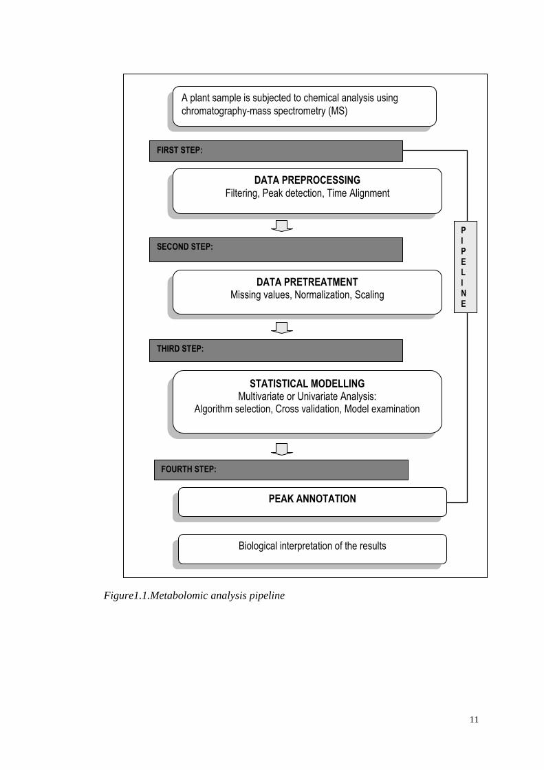
properties of the data. In this work I present a pre-processing, pre-treatment,
analysis and annotation pipeline for GC-MS and LC-MS metabolomic data
(Figure 1.1). This includes:
pre-processing (condensing and extracting features from the raw data);
pre-treatment (scaling and or normalization, to address specific properties of
the data)
statistical modelling (for example, dimensionality reduction and discriminant
analysis steps)
metabolite annotation (using appropriate databases)
11
Figure1.1.Metabolomic analysis pipeline
A plant sample is subjected to chemical analysis using
chromatography-mass spectrometry (MS)
DATA PREPROCESSING
Filtering, Peak detection, Time Alignment
DATA PRETREATMENT Missing values, Normalization, Scaling
STATISTICAL MODELLING Multivariate or Univariate Analysis:
Algorithm selection, Cross validation, Model examination
PEAK ANNOTATION
Biological interpretation of the results
FIRST STEP:
SECOND STEP:
THIRD STEP:
FOURTH STEP:
P I P E L I N E
12
Once a robust metabolomic analysis pipeline has been established, it can be used in
various applications; from answering simple biological questions (for example, what
are the differences between two cultivars?), to investigating complex metabolic
networks. The steps in the pipeline will now be considered individually.
1.3.1 Data pre-processing
In metabolomic analyses, a raw dataset may contain tens or hundreds of spectra,
each of them containing many hundreds or thousands of intensity measurements.
Low level pre-processing is often necessary in order to make sense of this large
volume of data. Data pre-processing constitutes the initial step in data handling
(Goodacre et al., 2007), and its main goal is to extract all the relevant information
from the raw data and summarize them in a single table (data matrix). This
procedure includes steps such as noise filtering, data binning, automatic peak
detection and chromatographic alignment.
Pre-processing mass spectrometric data is one of the most challenging areas in the
metabolomics field with regard to software development. Most of the technology
manufacturers provide automated software intended to accomplish these tasks for
instance AMDIS or SIEVE (Blackburn et al.; Styczynski et al., 2007), however,
instrument dependent software packages have substantial limitations and are usually
inefficient. Several free (open source) packages are increasingly being used in the
field, such as XCMS (Smith et al., 2006), MZMine (Katajamaa et al., 2006),
MetAlign (Lommen, 2009), and several others (Blackburn et al.). The pre-processing
step is discussed fully in Chapter 3.
1.3.2 Data pre-treatment
Certain properties of a dataset, such as unwanted technical variation can limit the
interpretability of metabolomics data (Van Den Berg et al., 2006; Werf et al., 2005).
Data pre-treatment methods are used to correct or at least reduce some of these
aspects (Idborg et al., 2005). Initially, data may be normalized prior to analysis to
remove certain types of systematic variations between the samples. Normalization
aims to remove this unwanted variation whilst preserving biological information.
There are several statistical methods for data normalization; one of the most common
is area normalization (Craig et al., 2006). When internal standards are added, their
13
peaks may be used as scaling factors for more efficient normalization (Sysi-Aho et
al., 2007).
Depending on the choice of statistical analysis method, the data may be further pre-
treated prior to model fitting. Mean centering and variance scaling are common pre-
treatment steps (Keun et al., 2003; Van Den Berg et al., 2006) that can optimize the
fit of the model to the data. Data pre-treatment is often overlooked, but in fact it can
have a great impact on the outcome of the statistical analysis. In this work it is
emphasized that pre-treatment is an important step of the analysis pipeline, and that
the assumptions and limitations of the pre-treatment method should always be taken
into account.
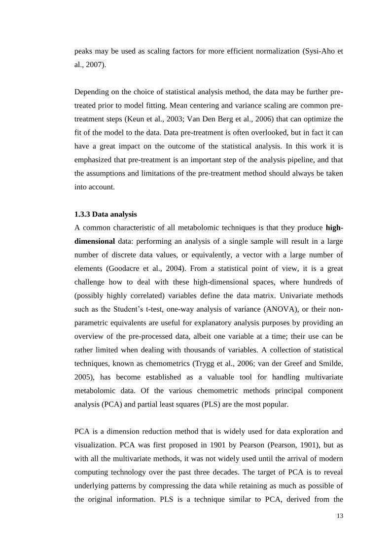
1.3.3 Data analysis
A common characteristic of all metabolomic techniques is that they produce high-
dimensional data: performing an analysis of a single sample will result in a large
number of discrete data values, or equivalently, a vector with a large number of
elements (Goodacre et al., 2004). From a statistical point of view, it is a great
challenge how to deal with these high-dimensional spaces, where hundreds of
(possibly highly correlated) variables define the data matrix. Univariate methods
such as the Student’s t-test, one-way analysis of variance (ANOVA), or their non-
parametric equivalents are useful for explanatory analysis purposes by providing an
overview of the pre-processed data, albeit one variable at a time; their use can be
rather limited when dealing with thousands of variables. A collection of statistical
techniques, known as chemometrics (Trygg et al., 2006; van der Greef and Smilde,
2005), has become established as a valuable tool for handling multivariate
metabolomic data. Of the various chemometric methods principal component
analysis (PCA) and partial least squares (PLS) are the most popular.
PCA is a dimension reduction method that is widely used for data exploration and
visualization. PCA was first proposed in 1901 by Pearson (Pearson, 1901), but as
with all the multivariate methods, it was not widely used until the arrival of modern
computing technology over the past three decades. The target of PCA is to reveal
underlying patterns by compressing the data while retaining as much as possible of
the original information. PLS is a technique similar to PCA, derived from the
14
concept of iterative fitting (Wold et al., 1983). In its basic regression form, PLS
models the relationship between two datasets, using a series of local least square fits.
This is the crucial difference between PLS and PCA: PLS is a supervised technique
that makes use of additional information to produce a statistical model, whereas PCA
is unsupervised not requiring a second data input.
An area that has attracted attention in the field is the use of metabolomic data for
mutant classification problems, discussed further below. Both PCA and PLS can
perform this kind of analysis when used as dimension reduction before discriminant
analysis, forming the methods PCA-DA and PLS-DA respectively. These
hyphenated methods are both highly effective supervised classification methods for
application to multivariate data. However, as with all supervised techniques
particular emphasis should always be given to model validation, as an important step
of the model building.
Regarding the statistical software for multivariate analysis, MATLAB is considered
a standard for the development and publication of chemometrics algorithms, while
the open source statistically-oriented language R is rapidly becoming a popular
alternative. These are the two development environments that have been used in the
present work. There are many other commercial and open source statistical packages
that offer options for multivariate analysis, including many with well-developed
graphical user interfaces (GUIs), e.g. SIMCA (Eriksson et al.; Wold and Sjostrom,
1977). However, where algorithm development or indeed transparency is a priority,
then a language-based package is the more flexible, preferred option.
1.3.4. Metabolite annotation
A big effort in the metabolomics field is directed towards the establishment of good
databases for the identification of plant metabolites (Bais et al., 2010). Although
substantial improvements have been made in the last years, the uniform annotation
of metabolite signals in publicly available databases remains a challenge (Saito and
Matsuda, 2010). The construction of metabolite databases in the plant field is
particularly difficult because plants produce a huge diversity of metabolites – larger
than that of animals and microorganisms. In fact, a single accession of Arabidopsis
thaliana is expected to produce ~5000 metabolites or more. AraCyc (Mueller et al.,
15
2003) is one of the most extensive databases that contains 2,632 compound entries to
date. Other databases that include plant metabolite data are KEGG (Okuda et al.,
2008), PlantCyc and KNApSAcK (Yonekura-Sakakibara and Saito, 2009).
In metabolomic studies, metabolite signals are identified by comparing their
chromatograms and mass spectra with those of standard compounds available in
libraries. However, the pool of identified compounds for some of the technologies
e.g. LC-MS, especially for secondary metabolites, is very much limited. Tandem MS
may be employed for structural elucidation in these cases. The most thorough
spectral libraries concern GC-MS technology. In the present work, the Golm
Metabolome Database (Hummel et al., 2007) was used for the annotation of GC-MS
data.
1.4 Applications of metabolomics in plant research
1.4.1 Functional genomics
Metabolomics as functional genomics tool aims to replace or complement the
somewhat laborious and low-throughput classical forward genetic approaches. The
key role of metabolomics in decoding the functions of genes has been reported
extensively in the recent years (Bino et al., 2004; Fiehn, 2002; Hagel and Facchini,
2008; Hall, 2006; Oksman-Caldentey and Saito, 2005). In plant systems,
metabolomics can be a valuable tool for the identification of responsible genes and
their products, or plant adaptations to different abiotic stresses. The detailed
characterization of metabolic adaptations to low and high temperature in Arabidopsis
thaliana has already demonstrated the power of this approach (Kaplan et al., 2004).
Metabolomics approaches have been successfully used to assess the natural variance
in metabolite content between individual plants, an approach with great potential for
the improvement of the compositional quality of crops (Fernie and Schauer, 2009;
Schauer and Fernie, 2006). The determination of the role of both metabolites and
genes can provide new ideas for genetic engineering and breeding.
1.4.2 Mutant analysis
The analysis of phenotypic mutants can greatly contribute to our understanding of
the structure and regulation of biosynthetic pathways in plants (Keurentjes, 2009).
Metabolomics, due to its unbiased approach, has become a major tool in the analysis
16
of direct transgenesis/mutation effects, as well as for the investigation of indirect and
potentially unknown alterations of plant metabolism. Metabolomics approaches have
been successfully used to phenotype genetically and environmentally diverse plant
systems, i.e. to determine the influence of transgenic and environmental
manipulations on a number of transgenic potato tubers altered in their starch
biosynthesis pathway, and wild type tubers incubated in different sugars using GC-
MS (Roessner et al., 2001). Many approaches for phenotypic analysis have been
described, ranging from changes in the whole plant phenotypes, or novel assays for
detecting specific compounds. The ultimate aim is to switch from specific classes of
molecule to more global metabolomics approaches.
The advancements in MS have allowed multiple compounds to be analysed
simultaneously, for example, LC-MS/MS analysis was efficiently used for the
screening of 10,000 Arabidopsis random mutant families for changes in levels of
free amino acids in seeds (Jander et al., 2004). The combination of mutants screening
and genetic mapping based identification can enhance the efficient discovery of
genes that influence enzymes in multiple pathways, of relationships between
different metabolites, and between metabolites and other traits.
The distinctiveness of mutant phenotypes was explored in a comparative analysis
that employed different fingerprinting technologies (NMR, GC-MS, LC-MS, FTIR)
and machine learning techniques (Scott et al., 2010). (The present thesis employs a
subset of the same data (the “HiMet” project, Chapter 4)). The use of metabolite
fingerprinting for the rapid classification of phenotypic Arabidopsis mutants has also
been reported (Messerli et al., 2007). Both of these studies demonstrated that
metabolomic analysis can successfully be used for the prediction of uncharacterized
mutants, in this way assisting in the process of gene discovery.
1.5 Further challenges in plant metabolomics
Considering the role of metabolites in biological systems, metabolomics can be a
very important tool in efforts to decipher plant metabolism. However, the
biochemical richness and complexity of plant systems will always remain one of the
fundamental challenges. Future directions in the field are set to involve the
improvement of the technological capabilities, the construction of public available

17
databases for plant metabolite annotation and finally the ultimate effort for systems
biology approaches that integrate analyses from metabolomics, transcriptomics and
proteomics experiments. Examples from studies in microorganisms show that this is
a promising research field, and such data sets are beginning to become available for
plant systems (Last et al., 2007; Redestig et al., 2011). In relation to the
establishment of a thorough data analysis pipeline, the ultimate goal of metabolomics
is to realize the full potential of technology and data handling methods, and leave
biological interpretation as the only real bottleneck remaining.

18
CHAPTER 2:
METABOLOMIC TECHNOLOGIES
19
2 METABOLOMIC TECHNOLOGIES
The development of high-throughput methods for measuring large numbers of
compounds has been facilitated in recent decades by rapid improvements in
analytical technologies. In order to enhance the information available from the
enormous amount of recorded (raw) data by the different analytical instruments, a
good understanding of the technologies used for the data acquisition is essential.
In this Chapter, I will present the technologies used to acquire the data in the present
work, along with a number of issues common to all the high-throughput analytical
techniques. In general terms, the capabilities of the different technologies to analyse
small molecules differ in the amount and type of compounds analysed per run, in the
quality of structural information they obtain, and in their sensitivity (Weckwerth,
2007). With regard to analysing the wide range of metabolites within a cell, each
technology provides particular advantages and disadvantages. There is no instrument
able to measure all compound classes involved in an ‘omic’ scale analysis (Dunn and
Ellis, 2005), therefore a combination of different technologies is often necessary to
gain a broad view of the metabolome of a tissue (Hollywood et al., 2006). The most
commonly used metabolomics techniques are chromatographic techniques coupled
to mass spectrometry (MS), and nuclear magnetic resonance (NMR). In this work,
the data were acquired by either Liquid Chromatography mass spectrometry (LC-
MS) or Gas Chromatography mass spectrometry (GC-MS), and they are discussed in
depth below.
2.1 The extraction method
Metabolomics presents a significant challenge for the extraction methodology, due to
the required comprehensiveness of the extract, which should represent as large
number of cellular metabolites as possible. Moreover, in order to have reproducible
measurements, the conditions and provenance of the biological material should be as
homogenous as possible in terms of environment (e.g. light, temperature, time of
sampling), and the enzymatic activity should be halted for the duration of the
extraction process to prevent possible degradation or inter-conversion of the
metabolites (Canelas et al., 2009; Lin et al., 2007; Moco et al., 2009).
20
The extraction method should also be adapted toward the analytical technique used
and the required metabolite range. No single extraction method is ideal for all the
metabolites within a cell or tissue. For metabolomics, with its implication of a
hypothesis-free design, a fast, reproducible and unselective extraction method is
preferred for detecting a wide range of metabolites. Wherever feasible, internal
standards can be added to the extraction solutions for quality control and for
subsequent quantification of the samples (Fiehn et al., 2008; Major and Plumb,
2006). Good analytical practice is also to conduct measurements on reference or
“quality control” (QC) samples at regular intervals during a study. The aim is to be
able to monitor and potentially correct for variations in the data due to changing
instrument response, an inevitability in virtually all analytical technologies.
2.2 Mass Spectrometry
The main requirement for metabolomic analysis is the ability of an instrument to
detect chemicals of complex mixtures with high accuracy. MS is ideal for this kind
of analysis because it can detect and resolve a broad range of metabolites with speed,
sensitivity and accuracy (Dettmer et al., 2007). It produces mass spectra with very
sharp peaks which to a great extent are independent of each other and reflect
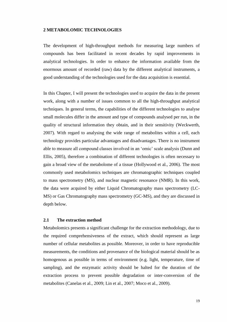
different metabolites. The key components of a mass spectrometer are shown in
Figure 2.1.
The data produced by mass spectrometric systems can be used in metabolomic
approaches without any knowledge of what chemicals are involved. However, mass
spectrometers can also be useful tools for subsequent structural identification of
unknown compounds. MS can be used to analyse biological extracts either directly
via direct-injection MS, or following chromatographic or electrophoretic separation.
(van Zijtveld et al., 2003). Direct injection mass spectrometry (DIMS) is a very rapid
technique to analyse large number of metabolites, but it has drawbacks mostly
because of a phenomenon known as ion suppression, where the signal of many
analytes can be lost at the mass spectrometer interface. For example, if one chemical
prevents ionisation of another, it may erroneously be concluded that the second is
absent. Moreover, without tandem MS (that involves multiple steps of
fragmentation), DIMS cannot distinguish isomers.
21
Figure 2.1.Basic diagram for a mass spectrometer
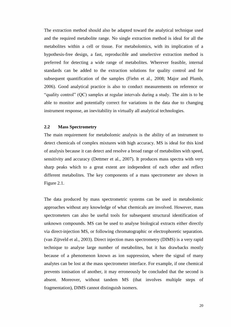
Figure2.2.The ion source consists of a heated filament giving off electrons. The
electrons are accelerated towards an anode and collide with the gaseous molecules
of the analyzed sample injected into the source.
e-
22
The first step for most of the techniques in mass spectrometry is the ionization of the
neutral molecules and the following decomposition of the molecular ions that are
produced. All these ions are separated according to their mass-to-charge ratio and are
detected in proportion to their abundance. Ultimately, the fragmentation products
provide information regarding the nature and the structure of the precursor molecule.
2.2.1 Ion Sources
An ion source (Figure 2.2) converts the gas or the liquid phase sample molecules
into ions. There are several techniques for the ionization of the samples prior to the
analysis in mass spectrometers. Some of them are very energetic and cause extensive
fragmentation, while others are softer and only produce molecular species. The
physicochemical properties of the analyte are very important at this stage, as it is
usually the ionization step that determines what types of samples can be analyzed by
mass spectrometry, i.e. some techniques are limited only to volatile and thermally
stable compounds.
Electron ionization and electrospray ionization (Figure 2.3) are very commonly used
in GC-MS and LC-MS analysis respectively (Cole, 1997). These two methods are
described in some more detail below. Others include: Field Desorption (FD), Plasma
desorption, laser desorption and Matrix Assisted Laser Desorption Ionization
(MALDI), fast atom bombardment (FAB), thermospray, atmospheric pressure
chemical ionization (APCI), thermal ionization (TIMS), and gas-phase ion molecular
reactions (De Hoffmann and Stroobant, 2007).
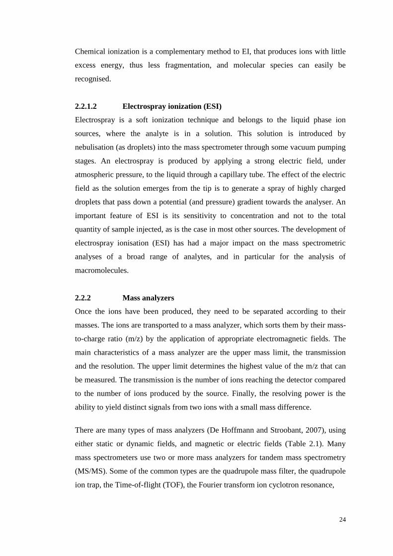
2.2.1.1 Electron ionization
Electron ionization is the most common form of ionization. It is suitable only for
gas-phase ionization, which requires that the compounds are sufficiently volatile.
Gases and samples with high vapour pressure are introduced directly into the source,
while liquids are heated in order to increase their vapour pressure. This technique
induces extensive fragmentation; the electron energy applied to the system is
typically 70 eV (electron Volts), with the result that molecular ions are not always
observed. Because of the extensive fragmentation, it works well for structural
identification of the compounds (Figure 2.4).
23
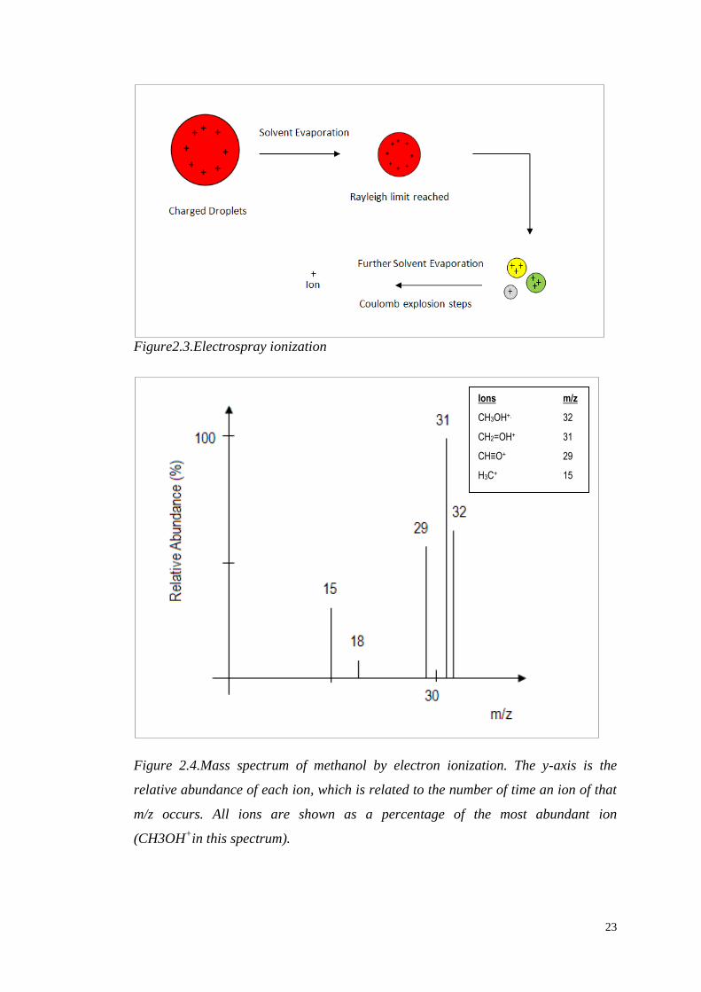
Figure2.3.Electrospray ionization
Figure 2.4.Mass spectrum of methanol by electron ionization. The y-axis is the
relative abundance of each ion, which is related to the number of time an ion of that
m/z occurs. All ions are shown as a percentage of the most abundant ion
(CH3OH+in this spectrum).
Ions m/z
CH3OH+. 32
CH2=OH+ 31
CH≡O+ 29
H3C+ 15
24
Chemical ionization is a complementary method to EI, that produces ions with little
excess energy, thus less fragmentation, and molecular species can easily be
recognised.
2.2.1.2 Electrospray ionization (ESI)
Electrospray is a soft ionization technique and belongs to the liquid phase ion
sources, where the analyte is in a solution. This solution is introduced by
nebulisation (as droplets) into the mass spectrometer through some vacuum pumping
stages. An electrospray is produced by applying a strong electric field, under
atmospheric pressure, to the liquid through a capillary tube. The effect of the electric
field as the solution emerges from the tip is to generate a spray of highly charged
droplets that pass down a potential (and pressure) gradient towards the analyser. An
important feature of ESI is its sensitivity to concentration and not to the total
quantity of sample injected, as is the case in most other sources. The development of
electrospray ionisation (ESI) has had a major impact on the mass spectrometric
analyses of a broad range of analytes, and in particular for the analysis of
macromolecules.
2.2.2 Mass analyzers
Once the ions have been produced, they need to be separated according to their
masses. The ions are transported to a mass analyzer, which sorts them by their mass-
to-charge ratio (m/z) by the application of appropriate electromagnetic fields. The
main characteristics of a mass analyzer are the upper mass limit, the transmission
and the resolution. The upper limit determines the highest value of the m/z that can
be measured. The transmission is the number of ions reaching the detector compared
to the number of ions produced by the source. Finally, the resolving power is the
ability to yield distinct signals from two ions with a small mass difference.
There are many types of mass analyzers (De Hoffmann and Stroobant, 2007), using
either static or dynamic fields, and magnetic or electric fields (Table 2.1). Many
mass spectrometers use two or more mass analyzers for tandem mass spectrometry
(MS/MS). Some of the common types are the quadrupole mass filter, the quadrupole
ion trap, the Time-of-flight (TOF), the Fourier transform ion cyclotron resonance,
25
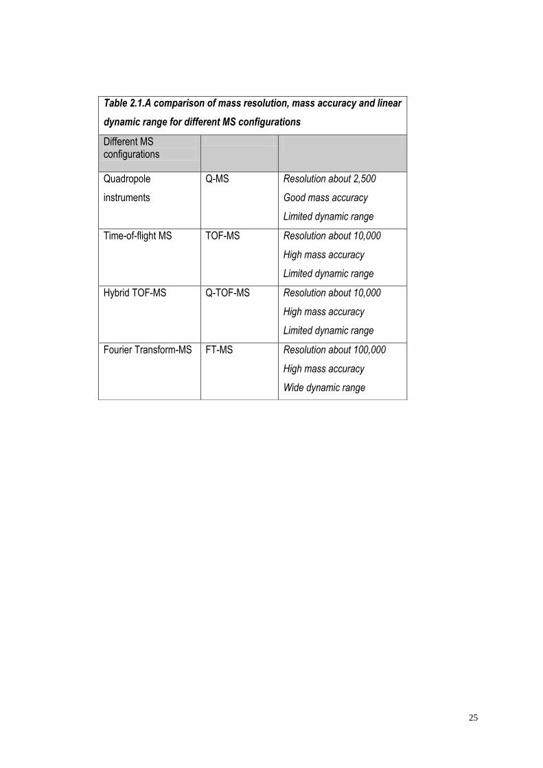
Table 2.1.A comparison of mass resolution, mass accuracy and linear
dynamic range for different MS configurations
Different MS configurations
Quadropole
instruments
Q-MS Resolution about 2,500
Good mass accuracy
Limited dynamic range
Time-of-flight MS TOF-MS Resolution about 10,000
High mass accuracy
Limited dynamic range
Hybrid TOF-MS Q-TOF-MS Resolution about 10,000
High mass accuracy
Limited dynamic range
Fourier Transform-MS FT-MS Resolution about 100,000
High mass accuracy
Wide dynamic range
26
and the Orbitrap. The first two are low-resolution, and the latter three high-resolution
analysers. Of the most common analyzers, which were used to acquire the data in the
present work, are the quadrupole and the ion trap.
2.2.2.1 The quadrupole
Quadrupole is a mass filter that produces an oscillating field created between four
parallel rods. A quadrupole mass analyzer acts as a mass-selective filter and only
ions with a given m/z range can pass through the system. Quadrupoles are low
resolution instruments. Usually, the quadrupoles are operated at unit resolution, i.e.
resolution that is sufficient to separate two peaks that are one mass unit apart.
2.2.2.2 Ion trap
The ion trap analyzer is a type of mass analyzer in which ions are confined in space
by means of a three-dimensional, rotationally symmetric quadrupolar electric field
capable of storing ions at selected m/z ratios. The ions are trapped in a quadrupole
field, in a space defined by the electrodes, and are sequentially ejected. It is also
possible to build a linear ion trap using quadrupoles, which is the case in the LTQ
(“linear trap quadrupole”) Orbitrap, for example.
2.2.3 Detectors
The final element of the mass spectrometer is the detector. The detector records
either the charge induced or the current produced when an ion passes by or hits a
surface. In a scanning instrument, it measures the value of an indicator of quantity
(the signal produced in the detector during the course of the scan versus where the
instrument is in the scan and produces a mass spectrum, representing the abundances
of each ion present as a function of m/Q.
2.2.4 Important MS Parameters
There are several instrumental parameters that describe the performance of a mass
spectrometer, which are used to determine whether the instrument suits the intended
analysis. The most important are the mass spectrometer’s resolving power and mass
accuracy. Mass resolution is the ability of the detector to distinguish two peaks of
slightly different m/z and it is described as the difference in mass-to-charge between
the two adjacent mass signals. Mass accuracy is used to indicate the deviation of the
27
instrument’s response from a known mass and it is described by the ratio of the mass
error and the expected mass:
( ) ( )
( )
where Δm is usually represented as parts per million, ppm. The quality and the
quantity of mass signals can be significantly improved by the using high-resolution
and ultra-high resolution accurate mass spectrometers.
The mass detector’s sensitivity and the linear dynamic range are also very important.
Mass sensitivity is the ability of an instrument to separate the intensity of a real
analyte from the noise. Sensitivity is given by the ratio between the intensity level of
the mass signal and the intensity level of the noise:
Linear dynamic range is the range over which the ion signal is linear with the analyte
concentration. In general, the development of new analytical techniques is largely
focused on increasing the resolution and the comprehensiveness of the metabolites
that are measured and on increasing the speed and throughput of the analytical
assays.
2.3 MS- chromatography coupling
The coupling of MS to chromatographic techniques enables the separation of the
mixture components before samples enter the mass spectrometer. By adding a
separation technique, the number of ions being measured at a given time is reduced,
which improves the analytical properties of the method by reducing ion suppression.
Moreover, chromatography can separate isomers, providing a way to measure
compounds with exactly the same mass. The separation properties usually reflect the
type of molecule being measured, i.e. polar versus hydrophobic or positively charged
versus negatively charged.
28
In the case of mass spectrometry-chromatography coupling, the instrument’s
resolving power in the time direction, i.e. a reasonably constant retention time scale,
is a very important prerequisite for obtaining consistent data that can be properly
combined across different sample acquisitions.
2.3.1 Gas Chromatography
GC-MS technology is highly suitable for rapid metabolite profiling, because it is a
very versatile technique which offers comprehensiveness for different compound
classes. Many applications have been developed for the most common plant
metabolites (Last et al., 2007). GC-MS is well established for chemical identification
and there is a large knowledge-base of literature and spectral libraries for all the
main metabolites (Schauer et al., 2005), the largest of which is the 2005
NIST/EPA/NIH Mass Spectral Library (http://www.nist.gov/srd/nist1.htm).
However, GC-MS has several limitations (Kopka, 2006). First of all, samples have
to be sufficiently volatile. Such compounds are introduced directly, but for non-
volatile components, chemical derivatization is required. Most metabolites analyzed
by GC-MS can be partitioned into polar and non-polar fractions, and after specific
derivatization, each fraction made volatile. There are a number of strategies for
derivatising compounds prior to GC/MS analysis, e.g. silylation, alkylation,
acylation and alkoxyamination, the standard procedure in plant metabolomics is to
first derivatise them using methoxyamine (CH3-O-NH2) in pyridine to stabilize
carbonyl moieties in the metabolites. Chemical derivatization provides significant
improvement in the compounds’ separation but has the drawback that it adds an
extra step into the analytical procedure, and it can introduce artefacts in the process,
for instance multiple derivatives of some compounds (e.g. amino acids) or
derivatives of reducing sugars.
GC-MS is most suited to small molecules. Large complicated molecules tend not to
be particularly volatile, and their derivatization is not easy. Measurements of higher
phosphates, co-factors and nucleotides have to be carried out using other techniques.
Moreover the analysis of secondary plant metabolites, and metabolites with relative
molecular masses exceeding m/z 600-800 is not feasible using GC-MS techniques.
Finally, samples are destroyed by the GC-MS sampling procedure.
29
2.3.2 Liquid Chromatography
Similar to gas chromatography MS (GC-MS), liquid chromatography mass
spectrometry (LC-MS) separates compounds chromatographically before they are
introduced into the mass spectrometer. It differs from GC-MS in that the mobile
phase is liquid, usually a mixture of water and organic solvents, instead of gas. LC-
MS most commonly uses soft ionization sources.
LC-MS is being increasingly used in metabolomics applications due to its high
sensitivity and the large range in analyte polarity and molecular mass it detects,
which is wider than GC–MS. LC–MS has a strong advantage over GC–MS (Díaz
Cruz et al., 2003), in that there is no need for chemical derivatization of metabolites
(required for the analysis of non-volatile compounds by GC–MS). A substantial
drawback for the LC–MS as a non-targeted profiling tool is the lack of transferable
mass spectral libraries. On the other hand, LC–MS can be a very good tool for
structural elucidation of unknown compounds, especially when it uses tandem MS.
2.4 Other technologies
Capillary electrophoresis (CE-MS) is an alternative MS technology used in
metabolomics, which has a very high resolving power and can profile simultaneously
many different metabolite classes (Terabe et al., 2001) .
Along with MS, NMR is one of the most important technologies in plant
metabolomics (Krishnan et al., 2005; Ratcliffe and Shachar-Hill, 2005). It can detect
a wide range of metabolites and provides both structural and quantitative results. It
has the great advantage that is a non-sample-destructive method. The main drawback
is that it provides lower sensitivity compared to other techniques regarding the
analysis of low abundance metabolites, thus it is not efficient for very complex
mixtures. For improved identification results the combination of NMR with MS can
be a very powerful strategy (Exarchou et al., 2003; Moco et al., 2007a).
Other alternatives include thin layer chromatography, FT-IR (Johnson et al., 2004)
and HPLC with ultraviolet (UV) but these give virtually no structural information.

30
2.5 Summary
The various metabolomics technologies provide different standards in analytical
precision, comprehensiveness and sample throughput. Each technique has particular
advantages in the identification and quantification of the metabolites in a biological
sample. LC-electrospray and NMR are considered as very important technologies in
the metabolomic race; LC-ESI for its coverage and sensitivity, NMR for its
coverage, resolution and structural aspects, especially where sensitivity is not the
main concern (e.g. concentrated medical samples versus dilute plants). However, the
comprehensiveness for different compound classes make GC-MS technology a
superior technique for plant metabolomics. Moreover GC-MS is quick, cheap, has
reasonable coverage, with good structural libraries, and was the technique of choice
for the major study reported in this thesis (Chapter 5), on starch metabolism in
Arabidopsis.

31
CHAPTER 3:
COMPUTATION
32
3 COMPUTATION
3.1 Pre-Processing – pipeline step 1
The first step in the data analysis pipeline is data pre-processing, which involves
aligning and peak extraction/integration processes that prepares the multiple samples
of raw data for the statistical modelling step. It is very important to perform this first
step diligently, since the accuracy and reproducibility of results from analysing LC-
MS and GC-MS data sets depend in part on careful data pre-processing.
Untargeted metabolite profiling yields a vast amount of complex data that can be
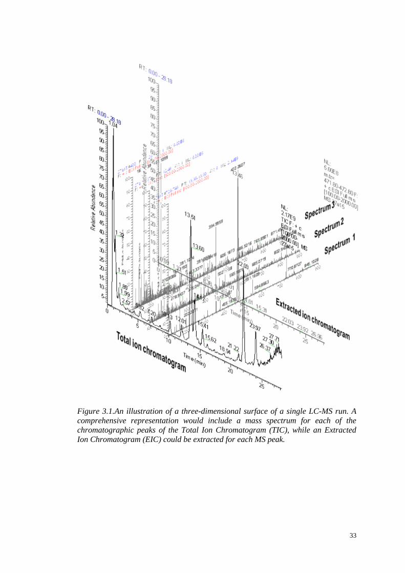
difficult to handle. Figure 3.1 shows an example of a three-dimensional surface of
LC-MS data that indicates the many components and the complexity of the nature of
the chromatographic data. Data pre-processing includes a variety of different
procedures for editing and analyzing mass spectrometric chromatographic data, such
as signal detection, spectral calibration, de-noising, baseline correction and
normalization (Bijlsma et al., 2006). The aim is to optimize the resulting matrix of
identified peaks and transform the data into a format that makes the subsequent
statistical analysis easier and more robust.
There are a number of tools for pre-processing MS-data, proposing different analysis
methods and algorithms; in this work I extensively used the XCMS software
(metlin.scripps.edu/xcms/). XCMS (Smith et al., 2006) has advanced capabilities for
feature selection, and is emerging as a very important resource in the metabolomics
field, not least because of its use of open source software (Corrado, 2005; Gentleman
et al., 2004). The XCMS software suite was developed initially for pre-processing
LC-MS data, and to our knowledge, it is used predominantly for this purpose.
However, with appropriate modification, it should also be highly useful for treating
GC-MS data. This approach is explored in the present work, in which I will disclose
the application of XCMS to GC-MS data, identifying the most important parameters
and the manner in which they need to be adjusted in order to optimize the pre-
processing step for this different class of data.
33
Figure 3.1.An illustration of a three-dimensional surface of a single LC-MS run. A
comprehensive representation would include a mass spectrum for each of the
chromatographic peaks of the Total Ion Chromatogram (TIC), while an Extracted
Ion Chromatogram (EIC) could be extracted for each MS peak.
34
3.1.1 XCMS – an overview
XCMS is a package developed in R (www.r-project.org) and made available by the
Bioconductor Project (http://www.bioconductor.org/), for the treatment of
(hyphenated) MS data. It is a sophisticated data analysis tool that includes many
options for data handling and visualization. It includes novel algorithms for data
analysis (Smith et al., 2006), taking advantage of the many statistical processing
routines available in R, whilst allowing the user to control its features in order to
optimise the analysis. However, because the software interface is a command line
programming environment, it can be a challenge for users without programming
experience.
In general terms, the XCMS software package transforms large, full-scan raw MS
data into a much smaller matrix of pre-processed data. XCMS has some prerequisites
regarding the input file formats. All data must be input in one of the following raw
file types: aia/andi, NetCDF, mzXML and mzData. In these file formats, the data are
stored as separate lists of mass/intensity pairs with each list representing one scan.
NetCDF (Rew and Davis, 1990), which has been used in the present work, is a very
common format and most MS instruments incorporate software for conversion to
this file type. XCMS outputs the final matrix of processed data into a tab separated
value (.tsv) file. This includes the intensity values for all masses (m/z values)
detected, for each one of the samples. The number of values can range from a few
hundred to a few thousand.
The pre-processed data may be subjected to further feature selection and subsequent
multivariate statistical analysis. XCMS offers some statistical processing, but this is
restricted to univariate ANOVA-type analyses on grouped data only (single grouping
variable). Furthermore, to utilise the XCMS statistical analysis features, data files
should be organised in subdirectories based on the sample grouping characteristics
e.g. cell type or mutation. More commonly, the final matrix of pre-processed is
output from XCMS and transferred to a dedicated package for statistical analysis (as
implemented in the present work).
The most important advantages of XCMS is that it works quickly, and crucially,
unlike the most common alternatives, it does not require the use of internal standards
35
for the retention time alignment (Elizabeth et al., 2006). The ability of its algorithms
to work without internal standards is very important. It is sometimes desirable to
avoid the addition of chemicals during sample preparation that may interfere with the
experimentally relevant metabolites. The isotopic and the adduct peaks are treated as
separate metabolite features, thus contributing to the total number of the identified
metabolites.
3.1.2 The XCMS environment
XCMS is implemented as an object-oriented framework within the R programming
environment. XCMS provides two main classes for data storage and processing,
respectively represented by the xcmsRaw and xcmsSet objects. Each class includes
several fixed algorithms and arguments that can be altered for the data analysis. The
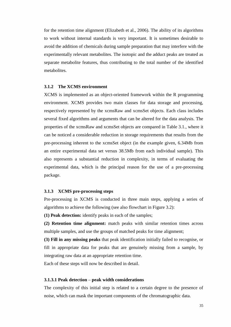
properties of the xcmsRaw and xcmsSet objects are compared in Table 3.1., where it
can be noticed a considerable reduction in storage requirements that results from the
pre-processing inherent to the xcmsSet object (in the example given, 6.34Mb from
an entire experimental data set versus 38.5Mb from each individual sample). This
also represents a substantial reduction in complexity, in terms of evaluating the
experimental data, which is the principal reason for the use of a pre-processing
package.
3.1.3 XCMS pre-processing steps
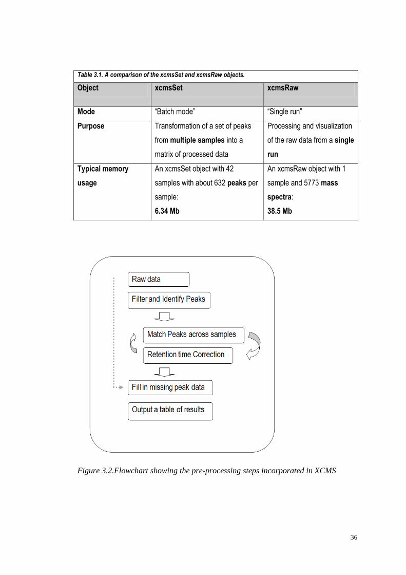
Pre-processing in XCMS is conducted in three main steps, applying a series of
algorithms to achieve the following (see also flowchart in Figure 3.2):
(1) Peak detection: identify peaks in each of the samples;
(2) Retention time alignment: match peaks with similar retention times across
multiple samples, and use the groups of matched peaks for time alignment;
(3) Fill in any missing peaks that peak identification initially failed to recognise, or
fill in appropriate data for peaks that are genuinely missing from a sample, by
integrating raw data at an appropriate retention time.
Each of these steps will now be described in detail.
3.1.3.1 Peak detection – peak width considerations
The complexity of this initial step is related to a certain degree to the presence of
noise, which can mask the important components of the chromatographic data.
36
Figure 3.2.Flowchart showing the pre-processing steps incorporated in XCMS
Table 3.1. A comparison of the xcmsSet and xcmsRaw objects.
Object xcmsSet xcmsRaw
Mode “Batch mode” “Single run”
Purpose Transformation of a set of peaks
from multiple samples into a
matrix of processed data
Processing and visualization
of the raw data from a single
run
Typical memory
usage
An xcmsSet object with 42
samples with about 632 peaks per
sample:
6.34 Mb
An xcmsRaw object with 1
sample and 5773 mass
spectra:
38.5 Mb
37
A good peak detection method should be able to reduce the noise and read complex
data in a comprehensive manner with the minimum loss of information. The XCMS
peak detection step provides a robust and reproducible method able to filter out
random noise and detect peaks with low signal-to-noise ratio.
The peak detection algorithm cuts the data into slices one tenth of a mass unit (0.1
m/z) wide, and then operates on the individual slices in the chromatographic domain.
Each of these slices is represented as an extracted ion chromatogram (EIC, see
Figure 3.1). Before peak detection, each slice is filtered with a “matched filter” that
uses a second derivative Gaussian shape to generate a new, smoothed
chromatographic profile. Match filtration is based on the application of a filter whose
coefficients are equal to the expected shape of the signal, to be discussed below
(Danielsson et al., 2002). After filtration, the peaks are detected using the mean of
the unfiltered data as a signal-to-noise cut-off. Finally, the peaks are determined by
integrating the unfiltered chromatogram between the zero-crossing points of the
filtered chromatogram. The most important parameters that need to be chosen at this
step are: the peak width of the filter, the boundaries of the mass tolerance window,
and the binning algorithm, which are each described below.
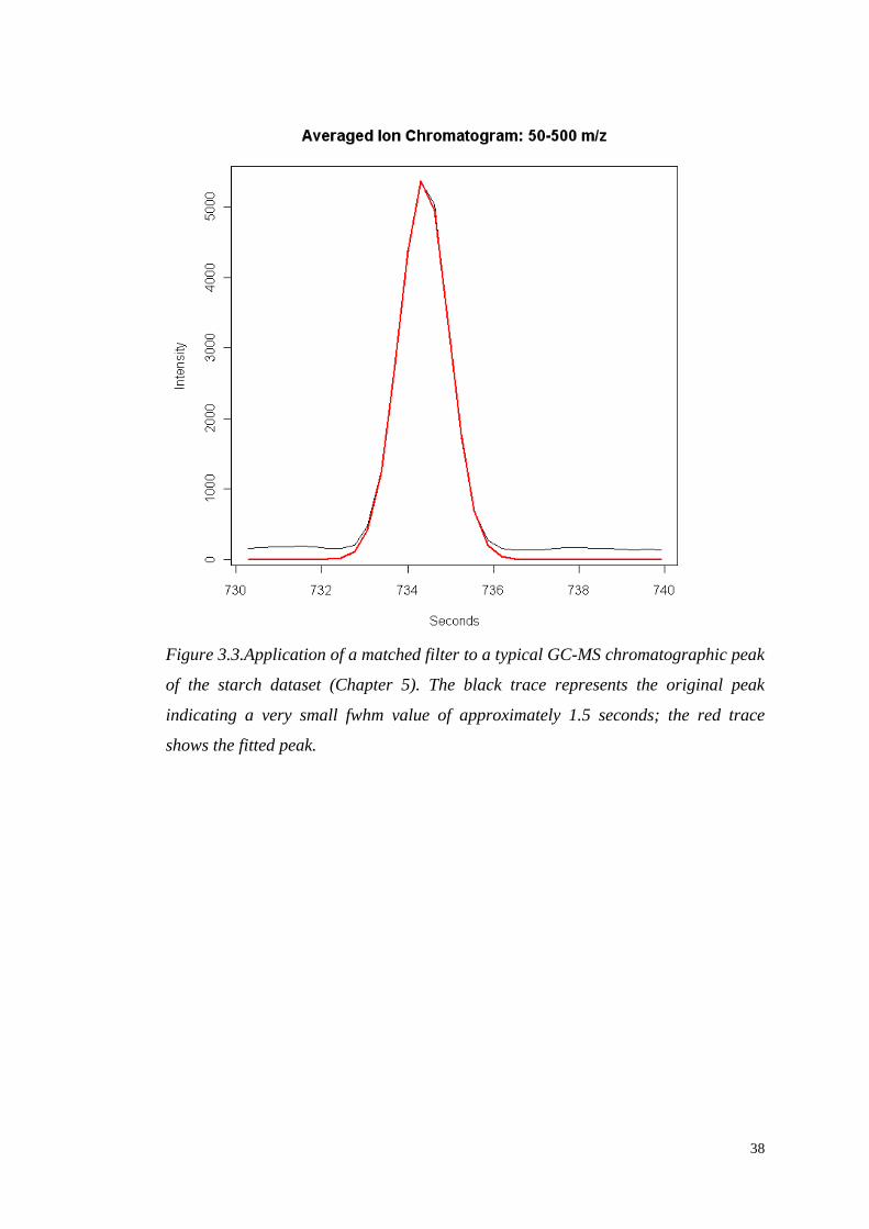
Peak width. The shape of a chromatographic peak can be very different
depending on the type of chromatography and the type of instrument. For
example, LC-MS peaks are much wider than those obtained by GC-MS and
TOF-MS. For the best use of the matched filter, the characteristics of the model
peak should fit the characteristics of the sample peak. The default XCMS value
for the peak full-width at half-maximum (fwhm) is 30 (seconds). Note that this is
appropriate for LC-MS, but not necessarily for the other techniques. In our work,
I established an optimal fwhm value of 3 to be used in processing the starch GC-
MS data set. The results are discussed in full Section 5.3.2, Figure 5.3; an
example of the filter applied to a representative GC-MS sample peak from our
data is shown in Figure 3.3.
Mass tolerance window (bin width). Another important consideration is the
relationship between the width of the mass peaks and the mass bin width, which
38
Figure 3.3.Application of a matched filter to a typical GC-MS chromatographic peak
of the starch dataset (Chapter 5). The black trace represents the original peak
indicating a very small fwhm value of approximately 1.5 seconds; the red trace
shows the fitted peak.
39
in turn is related to the resolution and scan-to-scan accuracy of the instrument. A
peak can shift or become distorted for two reasons. First, in high resolution
instruments or centroid mass spectral data, where the peak width can be
significantly smaller than the slice width, the signal from an analyte may sit
almost exactly on the boundary of two bins and oscillate between adjacent slices
over chromatographic time, making an otherwise smooth peak shape appear to
have a sharply uneven surface. In this case, the maximum signal intensity from
adjacent slices is combined into overlapping Extracted Ion Base Peak
Chromatograms (EIBPCs). Second, in low resolution instruments, where the
peak width can be larger than the default 0.1 m/z slice width, the signal from a
single peak may split across multiple slices and the middle of the very broad
peak (which is where the centroid line will be placed) will move around quite
widely. In this case, instead of eliminating the extra peaks during detection, the
algorithm incorporates a post-processing step where the full peak list is sorted
and examined by intensity, eliminating any low intensity peaks surrounding the
higher intensity peaks in a specific area. By altering the bin width, the XCMS
peak detection algorithm can handle, in theory, different peak shapes in a flexible
and robust manner.
Binning algorithm. The binning algorithm transforms the data from being
separate lists of mass and intensity pairs into a matrix with a row representing
equally spaced masses and a column for each sample. The software package
provides four alternative algorithms, which mainly differ in the way the intensity
in the mass bins is calculated, and the method used to interpolate areas with
missing data. In this work I used the default parameters for this step.
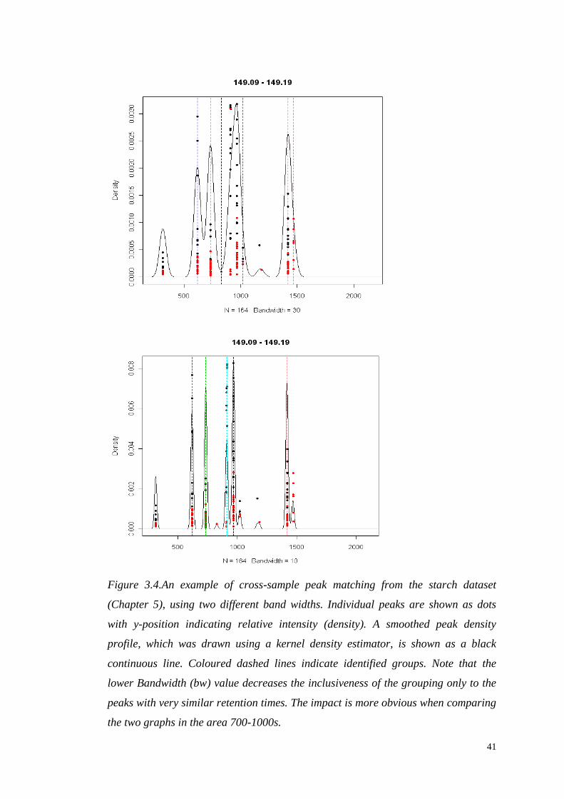
3.1.3.2 Retention time alignment – across samples peak grouping
Time alignment starts with the matching of peaks that represent the same analyte
across different samples. The matched peaks are subsequently used for the
calculation of retention times and alignment. The important parameter here is the
band width of peak groups (bw). The grouping algorithm starts with binning all the
samples in the mass domain. After grouping the peaks in bins, the algorithm resolves
groups of peaks with different retention times in each bin and starts to operate in the
40
chromatographic domain. To avoid certain complications, it uses a kernel density
estimator to calculate the overall distributions of peaks in chromatographic time
(Figure 3.4), and from these distributions identifies groups of peaks with similar
retention times. The algorithm employs several criteria for the optimum
identification of the groups, i.e. it selects only groups that contain more than half of
the samples. The effect of the grouping bandwidth can be seen in Figure 3.4.
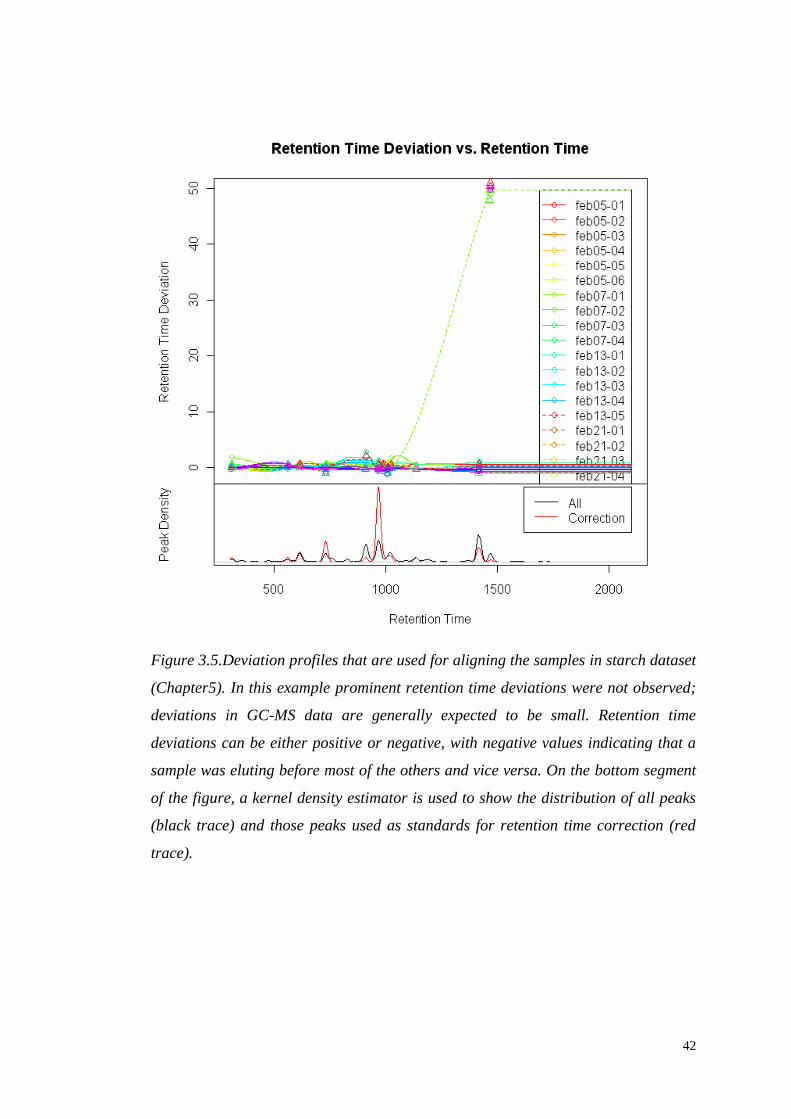
The grouping information from the peak matching step is used to identify groups of
peaks with a high probability of being well-matched, and these groups are used as
temporary standards. For every one of the so-called “well-behaved” groups, the
algorithm calculates the median retention time and the deviation from the median for
every sample in the group (Figure 3.5). For parts of the chromatogram in which no
well-behaved groups are identified, the algorithm uses a local regression fitting
model, “loess”, to approximate differences between deviations, and interpolates
sections where no peak groups are present. For increased precision, the alignment
step can be repeated recursively.
3.1.3.3 Filling missing peak data
XCMS includes a final step in which an algorithm identifies missing samples from
the groups, re-reads the raw data and integrates the regions of the missing peaks.
Missing samples from the groups can be a result of missed peaks during peak
identification, or because a peak is genuinely absent from a sample. This step is very
important because difficulties of handling missing values (or large numbers of zeros)
may arise in later statistical analysis.
3.1.4 Competing software
There are alternatives to XCMS for pre-processing MS data (Mueller et al., 2008).
Amongst the most popular of these are Sieve, MZmine, and MetAlign. Sieve is a
commercial software supplied by Thermofisher. It aligns chromatographic data,
extracts ion chromatograms (EICs) for every aligned ion and outputs them in a table.
Before the introduction of XCMS, Sieve was the only software used by the
Metabolite Services (JIC) for metabolomics analysis. Sieve (with a license to
Spotfire®) provides a very good user-friendly environment that allows interactive
41
Figure 3.4.An example of cross-sample peak matching from the starch dataset
(Chapter 5), using two different band widths. Individual peaks are shown as dots
with y-position indicating relative intensity (density). A smoothed peak density
profile, which was drawn using a kernel density estimator, is shown as a black
continuous line. Coloured dashed lines indicate identified groups. Note that the
lower Bandwidth (bw) value decreases the inclusiveness of the grouping only to the
peaks with very similar retention times. The impact is more obvious when comparing
the two graphs in the area 700-1000s.
42
Figure 3.5.Deviation profiles that are used for aligning the samples in starch dataset
(Chapter5). In this example prominent retention time deviations were not observed;
deviations in GC-MS data are generally expected to be small. Retention time
deviations can be either positive or negative, with negative values indicating that a
sample was eluting before most of the others and vice versa. On the bottom segment
of the figure, a kernel density estimator is used to show the distribution of all peaks
(black trace) and those peaks used as standards for retention time correction (red
trace).
43
visual inspection of the EICs, but it has some crucial flaws. First of all, it is
instrument dependent, compatible only with Thermofisher instruments. Moreover, it
does not allow access to its proprietary algorithms, thus it is difficult for the user to
fully understand how it works. The peak detection algorithms appear unrefined,
identifying peaks using unsophisticated thresh-holding processes which are often
inadequate.
MZmine (Katajamaa et al., 2006) is an open source package for the analysis of
metabolic MS data. It has good functionality, and allows the user to perform a large
amount of data pre-processing using EICs (Extracted Ion Chromatograms), and some
basic multivariate analysis. It has several visualization algorithms for both the raw
and processed data. The most important feature is the alignment tool, which can be
used to process data for export to allow analysis in other statistical software
packages. MetAlign (Lommen, 2009) is another very popular software programme
for the pre-processing and comparison of accurate mass and nominal mass GC-MS
and LC-MS data. Its algorithms incorporate several pre-processing steps i.e. data
smoothing, local noise calculation, baseline correction, between-chromatogram
alignment. It is capable of automatic format conversion and handling of up to 1000
data sets. Finally, many instrument manufacturers provide their own software
packages for metabolomic analysis. However, as noted for the Sieve package, such
proprietary software is in general instrument-specific and closed-source, so that the
numerical methods by which the data are pre-processed are not transparent.
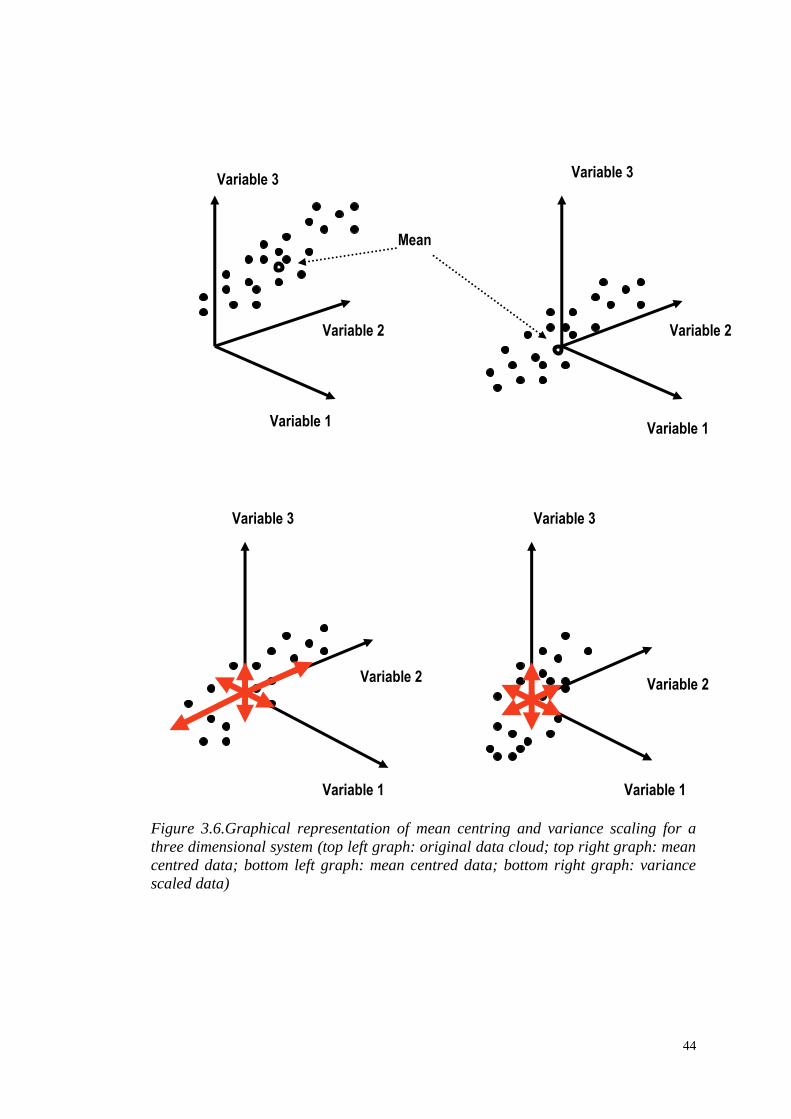
3.2 Pre-treatment – pipeline step 2
This step mainly concerns data scaling processes (mean centring, variance scaling,
normalization) and missing values treatment. Here, “scaling” is used to refer to
treatments which are applied column-wise (to each variable, or metabolite intensity):
for each variable, mean-centring simply consists of subtracting the dataset mean
from each intensity, and variance-scaling of dividing each intensity by the dataset’s
standard deviation. “Normalization” refers to treatments which are applied row-wise
(to each observation or sample), and principally this involves applying a correcting
factor so that the sum of all intensities equals unity, making overall intensity scales
comparable across samples. The choice of scaling requires a very careful
consideration, since scaling alters the relative distances between the observations
44
Figure 3.6.Graphical representation of mean centring and variance scaling for a
three dimensional system (top left graph: original data cloud; top right graph: mean
centred data; bottom left graph: mean centred data; bottom right graph: variance
scaled data)
Mean
Variable 1
Variable 2
Variable 3
Variable 1
Variable 2
Variable 3
Variable 1
Variable 2
Variable 3
Variable 1
Variable 2
Variable 3
45
(Figure 3.6), and this can have a dramatic effect on the output of analyses. Similarly
how one treats missing variables may have a significant effect on the position of
individual samples in clustering diagrams. The effect of these pre-treatments are
explored in detail in Chapter 4.
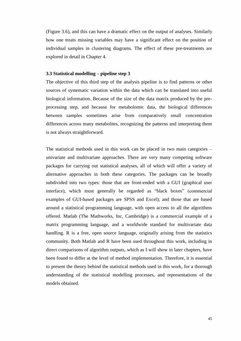
3.3 Statistical modelling – pipeline step 3
The objective of this third step of the analysis pipeline is to find patterns or other
sources of systematic variation within the data which can be translated into useful
biological information. Because of the size of the data matrix produced by the pre-
processing step, and because for metabolomic data, the biological differences
between samples sometimes arise from comparatively small concentration
differences across many metabolites, recognizing the patterns and interpreting them
is not always straightforward.
The statistical methods used in this work can be placed in two main categories –
univariate and multivariate approaches. There are very many competing software
packages for carrying out statistical analyses, all of which will offer a variety of
alternative approaches in both these categories. The packages can be broadly
subdivided into two types: those that are front-ended with a GUI (graphical user
interface), which must generally be regarded as “black boxes” (commercial
examples of GUI-based packages are SPSS and Excel); and those that are based
around a statistical programming language, with open access to all the algorithms
offered. Matlab (The Mathworks, Inc, Cambridge) is a commercial example of a
matrix programming language, and a worldwide standard for multivariate data
handling. R is a free, open source language, originally arising from the statistics
community. Both Matlab and R have been used throughout this work, including in
direct comparisons of algorithm outputs, which as I will show in later chapters, have
been found to differ at the level of method implementation. Therefore, it is essential
to present the theory behind the statistical methods used in this work, for a thorough
understanding of the statistical modelling processes, and representations of the
models obtained.
46
3.3.1 Multivariate analysis
PCA (principal component analysis) and PLS (partial least squares) are the most
commonly used techniques in the chemometrics field for analysing multivariate
(high-dimensional) data (Kemsley, 1996). Both of the methods compress the original
data matrix so that underlying patterns may be revealed. PCA is a very useful tool
for data visualization and exploration; PLS makes use of a second matrix of data (in
our case, categorical) to compress the data in a “supervised” manner. In this thesis,
PLS and PCA are used as dimension reduction methods in predictive models, prior
to linear discriminant analysis (PLS-DA, PCA-DA). The predictive capability of the
hyphenated models is evaluated using cross-validation. In Section 5.4.2.2 a direct
comparison between PCA-DA and PLS-DA is shown.
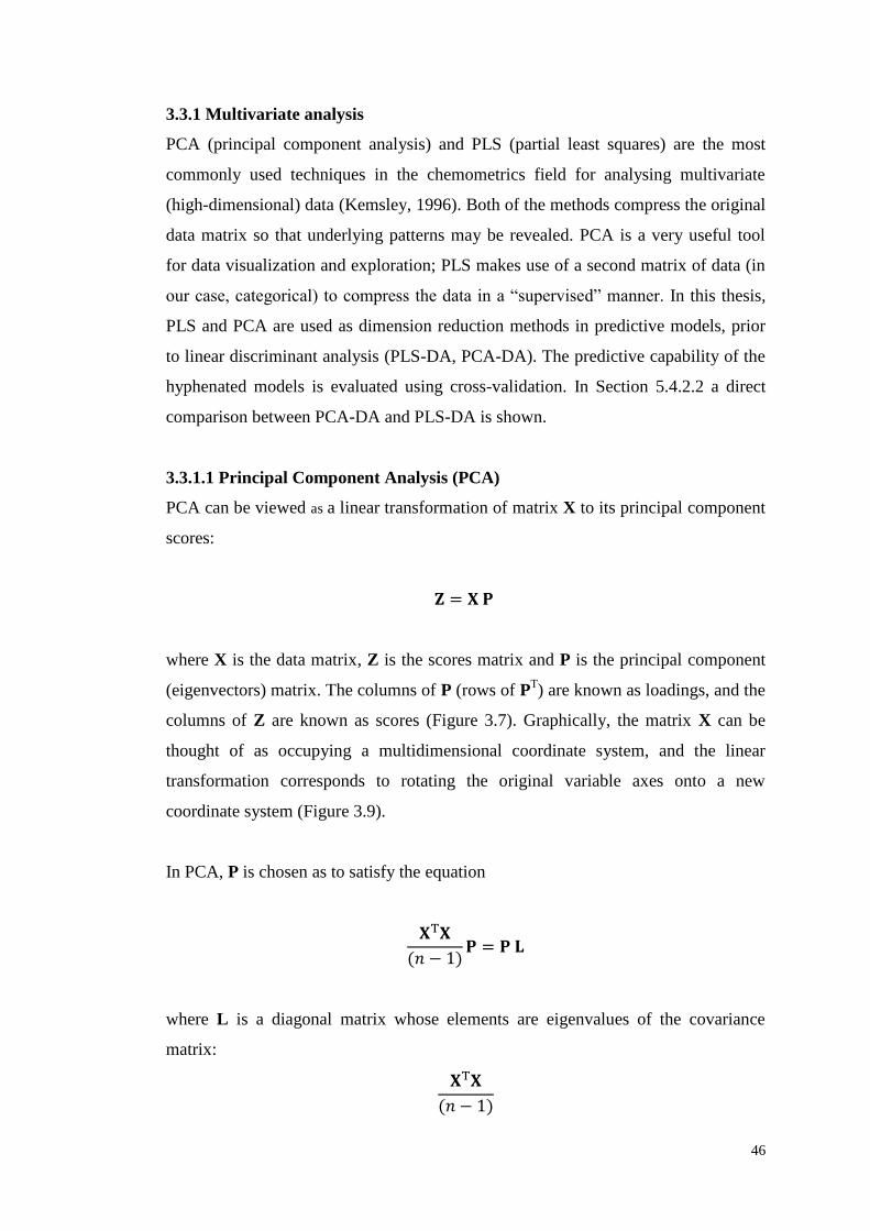
3.3.1.1 Principal Component Analysis (PCA)
PCA can be viewed as a linear transformation of matrix X to its principal component
scores:
where X is the data matrix, Z is the scores matrix and P is the principal component
(eigenvectors) matrix. The columns of P (rows of PT) are known as loadings, and the
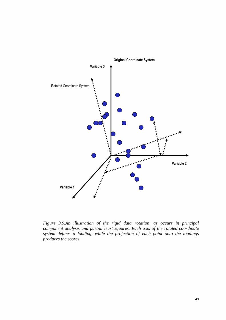
columns of Z are known as scores (Figure 3.7). Graphically, the matrix X can be
thought of as occupying a multidimensional coordinate system, and the linear
transformation corresponds to rotating the original variable axes onto a new
coordinate system (Figure 3.9).
In PCA, P is chosen as to satisfy the equation
( )
where L is a diagonal matrix whose elements are eigenvalues of the covariance
matrix:
( )
47
and the columns of P its corresponding eigenvectors. The eigenvalues also represent
the variance of the columns of Z. For many analysis methods the data matrix X is
mean-centred (column means subtracted from all entries).
There is also a formulation of PCA in which the X matrix is variance-scaled (the
mean-centred entries are divided by the respective column standard deviation), in
which case the loadings are eigenvectors of the data correlation matrix. Variance
scaling alters the relative distances between observations, thus the loadings and
scores will differ between the correlation and covariance matrix methods. In the
covariance matrix methods, the loadings retain the same units as the original data,
which can sometimes allow the analyst to attribute physical meaning to individual
PCs. However, in the correlation matrix method, small but potentially useful spectral
features can influence the linear transformation as much as large spectral peaks.
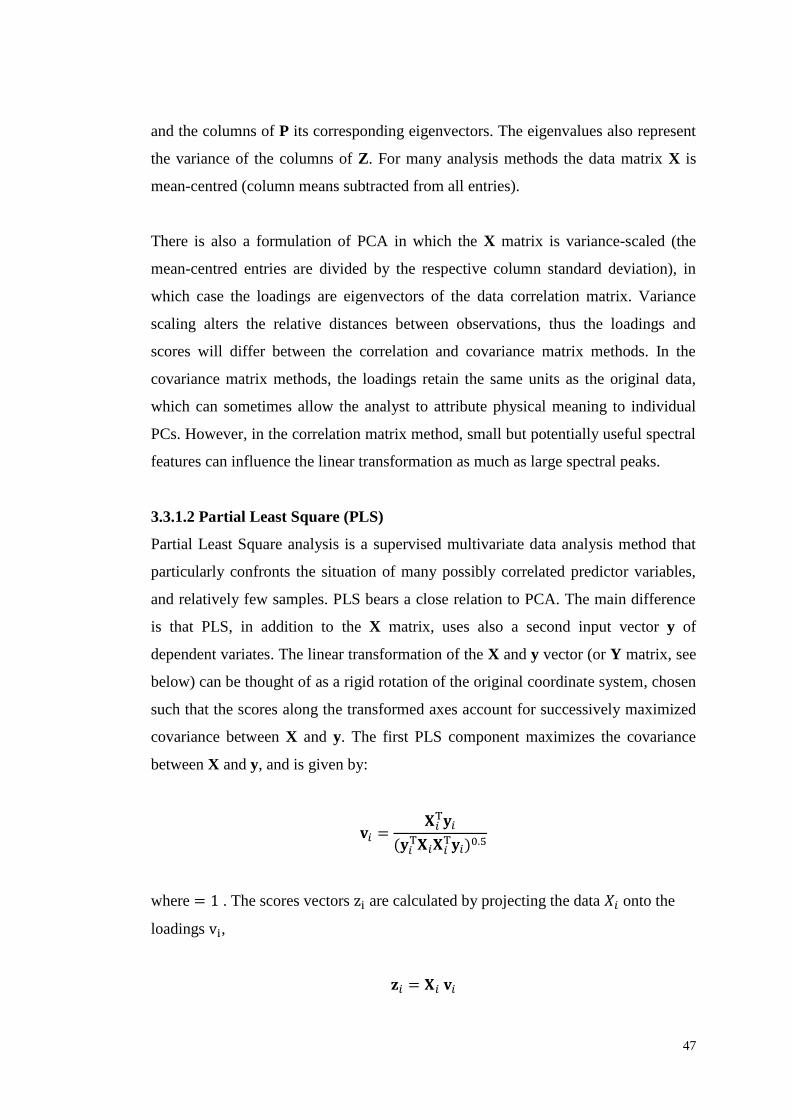
3.3.1.2 Partial Least Square (PLS)
Partial Least Square analysis is a supervised multivariate data analysis method that
particularly confronts the situation of many possibly correlated predictor variables,
and relatively few samples. PLS bears a close relation to PCA. The main difference
is that PLS, in addition to the X matrix, uses also a second input vector y of
dependent variates. The linear transformation of the X and y vector (or Y matrix, see
below) can be thought of as a rigid rotation of the original coordinate system, chosen
such that the scores along the transformed axes account for successively maximized
covariance between X and y. The first PLS component maximizes the covariance
between X and y, and is given by:
(
)
where . The scores vectors are calculated by projecting the data onto the
loadings ,
48
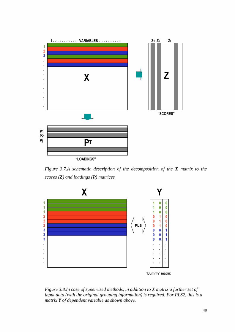
Figure 3.7.A schematic description of the decomposition of the X matrix to the
scores (Z) and loadings (P) matrices
Figure 3.8.In case of supervised methods, in addition to X matrix a further set of
input data (with the original grouping information) is required. For PLS2, this is a
matrix Y of dependent variable as shown above.
P1P2 Pj PT …
.
X
1 2 3 . . . . . . . . . . . . N
1 . . . . . . . . . . . . . . VARIABLES . . . . . . . . . . . . . . K
Z
….
Z1 Z2 Zi
“SCORES”
“LOADINGS”
X 1 1 1 2 2 2 3 3 3 . . . . . .
1 1 1 0 0 0 0 0 0 . . . . .
0 0 0 1 1 1 0 0 0 . . . . .
0 0 0 0 0 0 1 1 1 . . . . .
Y
PLS
‘Dummy’ matrix
49
Figure 3.9.An illustration of the rigid data rotation, as occurs in principal
component analysis and partial least squares. Each axis of the rotated coordinate
system defines a loading, while the projection of each point onto the loadings
produces the scores
Variable 2
Variable 1
Variable 3
Original Coordinate System
Rotated Coordinate System
50
The subsequent components are orthogonal (uncorrelated) to the previous
components. They are determined iteratively by calculating a residual-X and -y
(where the projected part of the data is subtracted from the complete dataset),
maximizing each time the covariance between the X-residual and y-residual. In our
work, a dummy matrix Y (rather than vector) is required to represent the different
groups or categories of data. In this case, the method is sometimes known as PLS2.
The original PLS method was first proposed in the 1980s, when computers were not
as advanced as today, and the algorithm had to make compromises at the coding
level in order for it to be practical to carry out the calculation of scores and loadings
in a reasonable time. Since then, various algorithms have been developed that
provide different definitions of PLS, some of which have the specific aim of
improving the speed of calculation (Andersson, 2009; de Jong, 1993; Geladi, 1988).
Both R and Matlab provide routines for carrying out PLS regression; additionally for
this work, in-house scripts have also been used for conducting the NIPALS PLS
method (Miyashita et al., 1990; Rosipal and Krämer, 2006). Some examples of
preliminary comparisons carried out in the different development environments are
given in Appendix A1, which presents Matlab and R scripts for conducting cross-
validated NIPALS PLS2. A Matlab in-house script for NIPAL PLS was applied to a
model dataset (infrared spectra of olive oils, publicly available at
www.ifr.ac.uk/Bioinformatics/BSDataSets.html) and the script outputs compared
with the original R version of PLS. This comparison resulted in a revision to the R
script, also shown, to correct for the absence of cross-validated scores amongst the
output arguments. Furthermore, in Chapter 5, I present the comparison of the output
from two different variants of PLS2 as applied to one of the metabolomics datasets
of interest. The methods in question are the NIPALS algorithm as described by
Martens (Martens, 2001) and the SIMPLS algorithm (de Jong, 1993) provided as the
PLS routine in Matlab).
3.3.1.3 Linear Discriminant Analysis (LDA)
Discriminant analysis is used to find the linear combination of features which best
separate two or more groups of observations. The LDA algorithms use the mean
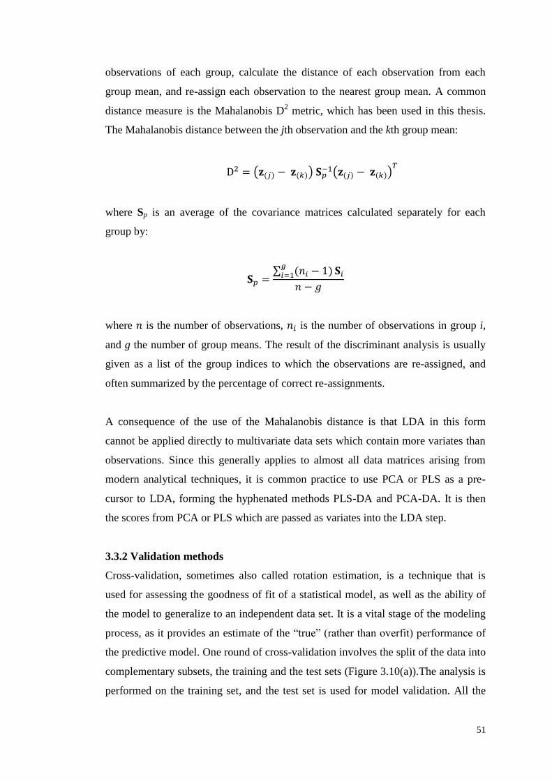
51
observations of each group, calculate the distance of each observation from each
group mean, and re-assign each observation to the nearest group mean. A common
distance measure is the Mahalanobis D2 metric, which has been used in this thesis.
The Mahalanobis distance between the jth observation and the kth group mean:
( ( ) ( )) ( ( ) ( ))
where Sp is an average of the covariance matrices calculated separately for each
group by:
∑ ( )
where is the number of observations, is the number of observations in group i,
and g the number of group means. The result of the discriminant analysis is usually
given as a list of the group indices to which the observations are re-assigned, and
often summarized by the percentage of correct re-assignments.
A consequence of the use of the Mahalanobis distance is that LDA in this form
cannot be applied directly to multivariate data sets which contain more variates than
observations. Since this generally applies to almost all data matrices arising from
modern analytical techniques, it is common practice to use PCA or PLS as a pre-
cursor to LDA, forming the hyphenated methods PLS-DA and PCA-DA. It is then
the scores from PCA or PLS which are passed as variates into the LDA step.
3.3.2 Validation methods
Cross-validation, sometimes also called rotation estimation, is a technique that is
used for assessing the goodness of fit of a statistical model, as well as the ability of
the model to generalize to an independent data set. It is a vital stage of the modeling
process, as it provides an estimate of the “true” (rather than overfit) performance of
the predictive model. One round of cross-validation involves the split of the data into
complementary subsets, the training and the test sets (Figure 3.10(a)).The analysis is
performed on the training set, and the test set is used for model validation. All the
52
model parameters, i.e. the optimum number of components and the selected
variables, are optimized on the training set. To reduce variability, multiple rounds of
cross-validation are performed using different partitions, and the validation results
are averaged over the rounds.
The differences between the various cross-validation types are based on differences
of the sub-set partitioning process. In this work, leave-one-out and leave-segment-
out cross validation was used. Both of the methods differ from repeated random
partitioning in that all observations are used as both training and tests sets and each
observation is used as a test set exactly once. In leave-segment-out (K-fold) cross-
validation (Figure 3.10(b)), the original dataset is randomly partitioned into K
subsets. A single subset is used as a test set and the remaining are used as training
set. The cross-validation process is repeated K-times and each of the subsets is used
exactly once as validation set. In leave-one-out cross-validation (LOOCV) a single
observation from the original data set is used as test set, and the remaining
observations as training set. This is repeated such that each observation in the sample
is used once as test item. The various cross-validation methods are advantageous in
situations where the number of independent observations in the dataset is relatively
small (i.e., tens rather than hundreds), but they need to be used appropriately and
with an awareness of their limitations. The choice of an inappropriate validation
method can lead to overfitting, a phenomenon which is examined in Section 4.4.1.
3.3.3 Univariate analysis
Univariate statistical analysis encompasses the wide range of traditional statistical
methods in which only one predictor variable is considered at a time. In the context
of metabolomics data analysis, univariate analysis is often used in the first stages of
research for descriptive purposes, where individual metabolites are viewed (and
sometimes modeled) singly, or also as a confirmatory tool following multivariate
analysis. Generally though, it is supplemented by more advanced multivariate
statistical methods. The focus of the present work is the application of multivariate
techniques for the analysis of high-dimensional data. However, some selected
univariate analysis methods (specifically, multi-way ANOVA (in Chapter 5) and
non-parametric equivalents of t-tests (Chapter 4)) are used for comparative purposes,
and these will be described briefly first.
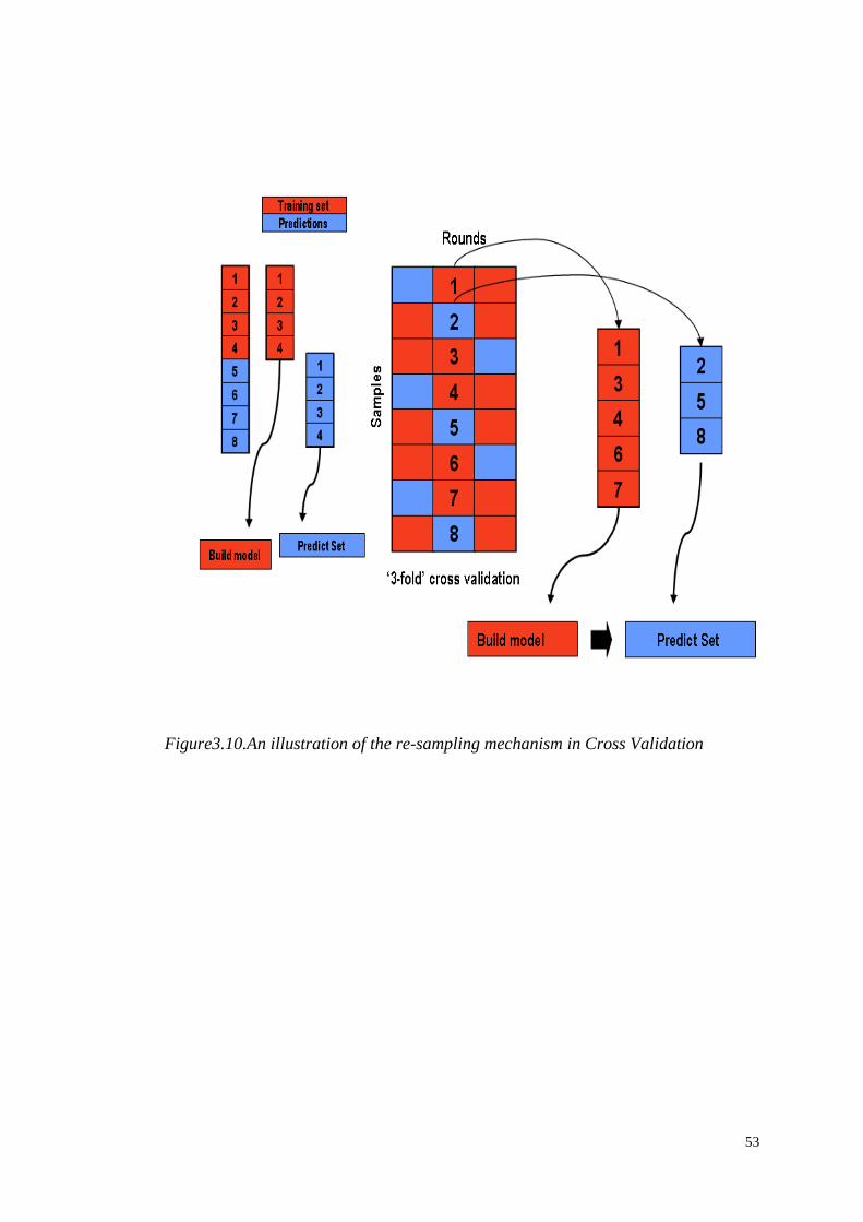
53
Figure3.10.An illustration of the re-sampling mechanism in Cross Validation

54
3.3.3.1 Analysis of variance (ANOVA)
ANOVA is a technique that aims to discover whether data from nominally different
groups are statistically different, that is, to determine whether the groups differ
significantly with respect to the measured characteristic. It does this by testing the
null hypothesis that the groups share a common mean.
The standard ANOVA output is a table containing elements as follows: sums of
squares (SS), degrees of freedom (df), mean squares (SS/df), F statistic, and p-value
(Figure 3.11). The F statistic is used in the hypothesis test, and the p-value returned
informs on the significance. A small p-value is evidence for rejecting the null
hypothesis, and suggests that the group means are significantly different. The p-
value depends on assumptions about the random disturbances in the model equation.
For the p-value to be valid, these disturbances need to be independent, normally
distributed, and have uniform variance.
Figure 3.11.Multi-way ANOVA table for two factors X1(day of analysis) and
X2(genotype). The p-value (Prob>F) for X2 indicates whether or not the type of
genotype is a significant factor for separating the groups of samples after
compensating for the effect of day. This is an example from section 5.4.1., showing
that one of the identified spectral features (a peak with m/z 130 and retention time
11.35min) is not a discriminatory factor for the five genotypes involved in the
experiment.
55
Multi-way (N-way) ANOVA is used to determine whether the means in a set of data
differ when grouped by multiple factors, and indicate which factors or combinations
of factors are associated with the difference. For example in Chapter 5, these factors
are the different genotypes as well as the day that the analysis was performed.
A graphical reassurance that the means of groups are different for each examined
variable can be gained by looking at the boxplots (this is the way I will examine the
variables in Section 5.4.1.2). However, it should be noted that the notches are (by
default in this software package) used for a comparison of medians, not a
comparison of means.
3.3.3.2 Multi-comparison tests
Post-hoc multi-comparison tests are performed to determine not just whether there
are any differences among the means, but specifically to assess which pairs of means
are significantly different. The several available tests differ on the assumptions about
characteristics of the statistical population. In this thesis I used two types of tests: the
parametric Student’s t-test and the non-parametric Wilcoxon signed-rank test.
Students t-test examines if two independent samples that come from normal
distributions with unknown but equal (or, optionally, unequal) variances have the
same mean, against the alternative that the means are unequal. In a t test, a t statistic
is computed and compared to a critical value. The critical value is chosen so that
when the means are the same (any difference is attributed to random chance), the
probability that the t statistic will exceed the critical value is small (i.e. less than 5%,
a commonly used threshold for the p-value). In Section 5.4.2.2, the critical values
from the t distribution are calculated using a Bonferroni adjustment to compensate
for multiple comparisons. The Bonferroni adjustment at the 5% level is calculated
as:
( ) ⁄
A Wilcoxon rank sum test examines if two independent samples that come from
identical continuous distributions have equal medians, against the alternative that
they do not have equal medians. It is the non-parametic equivalent of the t-test. The

56
key difference is that the data are not used in their raw form, but are instead
transformed into a ranked list before calculation of the test statistics. In this way, the
distribution of the original data is irrelevant as far as the test is concerned (hence the
term “non-parametric”).
3.4 Peak annotation – pipeline step 4
The final step in the metabolomics data pipeline is annotation of the individual
peaks. Comprehensive identification of all detected metabolites is a challenging task;
however, if the output from the statistical analysis includes, for instance, a subset or
a ranked list of important peaks, then the task of annotation can be made less
daunting by reducing the scale of the task.
In the present work, for the annotation of peaks I used AMDIS software, where
metabolites are identified by comparing retention indices and mass spectra with the
Golm Metabolome Database and NIST libraries. The data are imported in NetCDF
format; an automated calibration process is run that converts the retention times to
retention index values; and subsequently, within a few seconds, the software package
outputs a list of identified compounds.

57
CHAPTER 4:
CONSIDERATIONS FOR METABOLOMICS DATA
ANALYSIS: A CASE STUDY – THE HiMet PROJECT
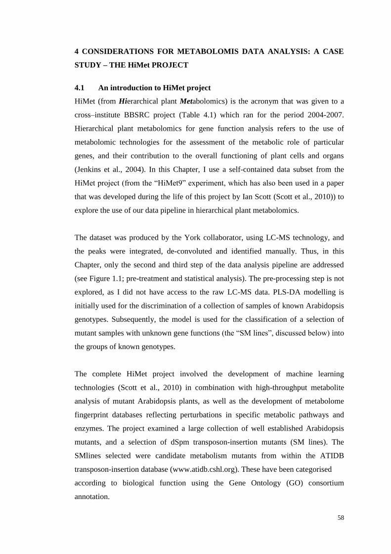
58
4 CONSIDERATIONS FOR METABOLOMIS DATA ANALYSIS: A CASE
STUDY – THE HiMet PROJECT
4.1 An introduction to HiMet project
HiMet (from Hierarchical plant Metabolomics) is the acronym that was given to a
cross–institute BBSRC project (Table 4.1) which ran for the period 2004-2007.
Hierarchical plant metabolomics for gene function analysis refers to the use of
metabolomic technologies for the assessment of the metabolic role of particular
genes, and their contribution to the overall functioning of plant cells and organs
(Jenkins et al., 2004). In this Chapter, I use a self-contained data subset from the
HiMet project (from the “HiMet9” experiment, which has also been used in a paper
that was developed during the life of this project by Ian Scott (Scott et al., 2010)) to
explore the use of our data pipeline in hierarchical plant metabolomics.
The dataset was produced by the York collaborator, using LC-MS technology, and
the peaks were integrated, de-convoluted and identified manually. Thus, in this
Chapter, only the second and third step of the data analysis pipeline are addressed
(see Figure 1.1; pre-treatment and statistical analysis). The pre-processing step is not
explored, as I did not have access to the raw LC-MS data. PLS-DA modelling is
initially used for the discrimination of a collection of samples of known Arabidopsis
genotypes. Subsequently, the model is used for the classification of a selection of
mutant samples with unknown gene functions (the “SM lines”, discussed below) into
the groups of known genotypes.
The complete HiMet project involved the development of machine learning
technologies (Scott et al., 2010) in combination with high-throughput metabolite
analysis of mutant Arabidopsis plants, as well as the development of metabolome
fingerprint databases reflecting perturbations in specific metabolic pathways and
enzymes. The project examined a large collection of well established Arabidopsis
mutants, and a selection of dSpm transposon-insertion mutants (SM lines). The
SMlines selected were candidate metabolism mutants from within the ATIDB
transposon-insertion database (www.atidb.cshl.org). These have been categorised
according to biological function using the Gene Ontology (GO) consortium
annotation.
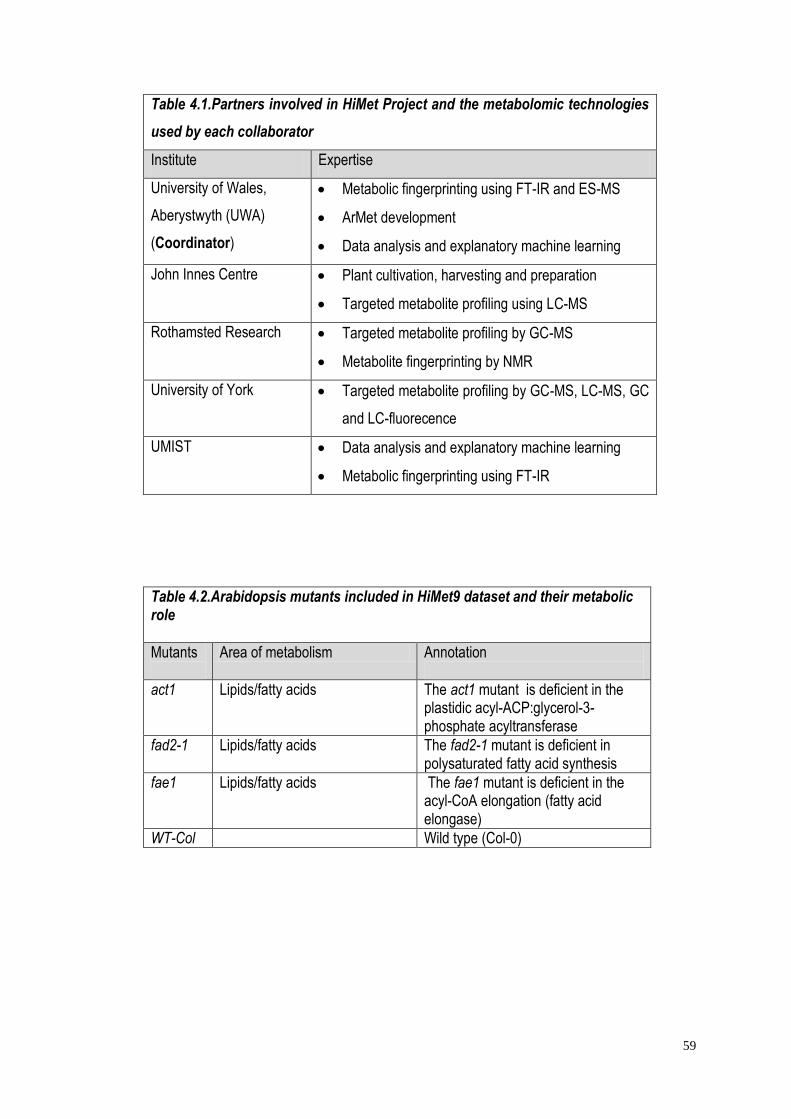
59
Table 4.1.Partners involved in HiMet Project and the metabolomic technologies
used by each collaborator
Institute Expertise
University of Wales,
Aberystwyth (UWA)
(Coordinator)
Metabolic fingerprinting using FT-IR and ES-MS
ArMet development
Data analysis and explanatory machine learning
John Innes Centre Plant cultivation, harvesting and preparation
Targeted metabolite profiling using LC-MS
Rothamsted Research Targeted metabolite profiling by GC-MS
Metabolite fingerprinting by NMR
University of York Targeted metabolite profiling by GC-MS, LC-MS, GC
and LC-fluorecence
UMIST Data analysis and explanatory machine learning
Metabolic fingerprinting using FT-IR
Table 4.2.Arabidopsis mutants included in HiMet9 dataset and their metabolic role
Mutants
Area of metabolism Annotation
act1 Lipids/fatty acids
The act1 mutant is deficient in the plastidic acyl-ACP:glycerol-3-phosphate acyltransferase
fad2-1 Lipids/fatty acids
The fad2-1 mutant is deficient in polysaturated fatty acid synthesis
fae1 Lipids/fatty acids
The fae1 mutant is deficient in the acyl-CoA elongation (fatty acid elongase)
WT-Col Wild type (Col-0)
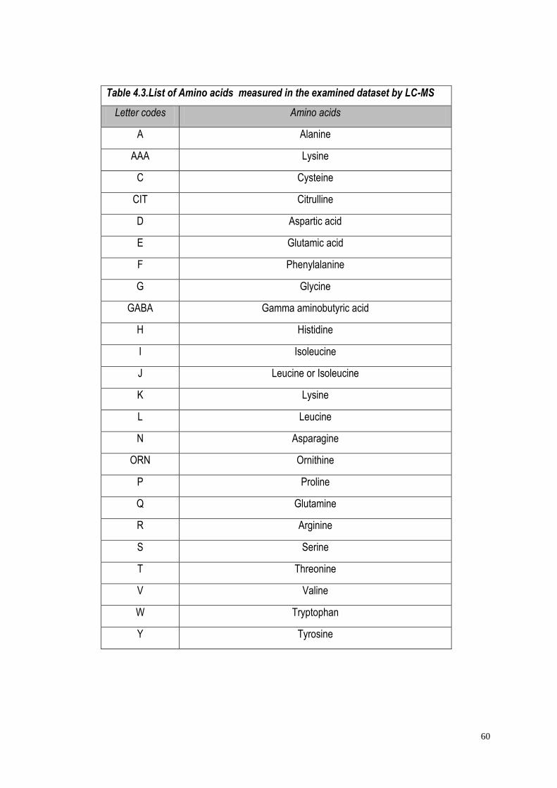
60
Table 4.3.List of Amino acids measured in the examined dataset by LC-MS
Letter codes Amino acids
A Alanine
AAA Lysine
C Cysteine
CIT Citrulline
D Aspartic acid
E Glutamic acid
F Phenylalanine
G Glycine
GABA Gamma aminobutyric acid
H Histidine
I Isoleucine
J Leucine or Isoleucine
K Lysine
L Leucine
N Asparagine
ORN Ornithine
P Proline
Q Glutamine
R Arginine
S Serine
T Threonine
V Valine
W Tryptophan
Y Tyrosine
61
4.2 Materials and methods
4.2.1 Samples
The dataset’s known-genotype samples (Table 4.2) include the wild-type (WT-Col),
and three Arabidopsis lipid/fatty acid mutants: act1 mutant - deficient in the plastid
acyltransferase that catalyzes lysophosphatidic acid biosynthesis; fad2-1 mutant –
deficient in polyunsaturated fatty acid synthesis; and fae1 mutant – related to fatty
acid elongation. Additionally, a collection of eleven SM single-copy transposon-
insertion lines (SM 15225, SM 15771, SM 17367, SM 18958, SM 19779, SM 19801,
SM 19881, SM 20192, SM 21150, SM 270, SM 35810) was used to investigate
previously unknown gene functions. These SM lines were selected via a TIGR.5
genome annotation of the ATIDB database, and the ATIDB entries were matched to
MAPMAN for Gene Ontology Consortium categorization.
4.2.2 Plant growth and harvest
Plants were grown by the JIC partner in nine random blocks in an environment of
23°C/18°C, 16/8 h day/night photoperiods of 250 to 270 mmol m-2
s-1
light, and 70%
relative humidity. Aerial tissues from stage 6.00 plants (Boyes et al., 2001) were
harvested into liquid N2 in mid light period, freeze dried, and powdered. Replicate
plants from each block were allocated to each analytical method. Shipment and
laboratory processing entailed a few days at ambient temperature.
4.2.3 Sample analysis
Twenty-four amino acids were measured by the York partner, with norleucine used
as an internal standard, on a Thermo LCQ Classic LC-MS device (Thermo
Scientific). Samples (2 mg) extracted in 70 μL of 80:20 ethanol:water (4°C, 30 min)
were analyzed as isobutyl chloroformate derivatives (Husek, 1998) on a 100 mm
porous graphitic column (5 mmHypercarb; Thermo Scientific) at 0.4 mL min-1
with
a 15min gradient of 100% solvent A (10 mM ammonium trifluoroacetate, 10 mM
trifluoroacetic acid in 50:50 ethanol:water) to 100% B (10 mM trifluoroacetic acid in
tetrahydrofuran). Amino acids were measured by positive-ion atmospheric pressure
chemical ionization-tandem MS, with capillary at 4V and 150°C, vaporizer at 550°C,
and discharge current of 6 mA (Scott et al., 2010).
62
4.3 Multivariate data exploration and pre-treatment
4.3.1 The raw data
All pre-processing (peak identification and integration) was carried out by the
collaborators at York. The raw data matrix of the specific dataset incorporates the
intensities of 24 amino acids (Table 4.3) for 105 samples. These 105 observations
include the four genotypes (act1, fad2-1 and fae1 mutants, and the wild type), and
consist of 9 independent biological replicates for each of the wild-type, act1 and
fad2-1 mutants, 8 independent biological replicates of fae1 mutant, and three
technical replicates for each biological replicate (identified by unique sample codes).
(see Appendix A2, Table 4.4).
It is good practice to use an appropriate way of examining the raw data in its
entirety, as an initial means of quality control. Many different types of graphs can be
used for this purpose, but amongst the most useful are the “heatmap” representations
which make use of colour to represent intensities in the dataset. The complete table
of raw data is shown as a heatmap in Figure 4.1. In this type of plot, each data value
(metabolite intensity) is indicated by a patch of colour whose RGB (red-green-blue)
value has been determined by mapping the intensity value onto the desired colour
scale. Heatmaps of the intensity matrices provide an immediate impression of the
general patterns in the data. For instance, it is apparent that the HiMet 9 data
matrices are dominated by two amino acids, E (Glutamate) and Q (Glutamine).
4.3.2. Missing values
Missing values (i.e. empty cells where the respective metabolite has not been
assigned to any numerical value) are very common phenomena in metabolomic
measurements. The handling of missing values is an important step in the
preparation of the data, as most of the multivariate methods require a fully defined
matrix, or become computationally ineffective for incomplete data. How best to deal
with sets containing missing values depends in part on the actual number of missing
values and also, if there is an indication, on the mechanism which gave rise to them.
For instance, missing values sometimes imply that the level of the respective
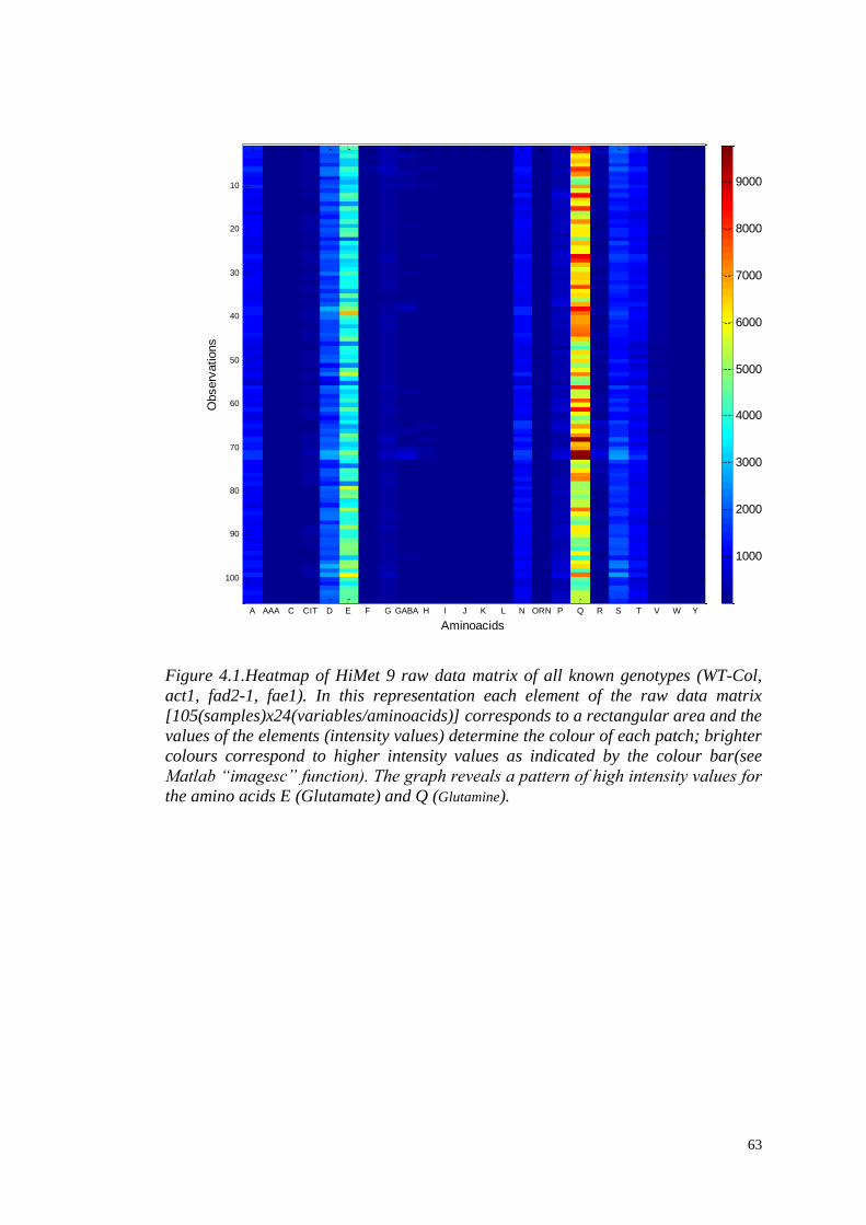
63
Figure 4.1.Heatmap of HiMet 9 raw data matrix of all known genotypes (WT-Col,
act1, fad2-1, fae1). In this representation each element of the raw data matrix
[105(samples)x24(variables/aminoacids)] corresponds to a rectangular area and the
values of the elements (intensity values) determine the colour of each patch; brighter
colours correspond to higher intensity values as indicated by the colour bar(see
Matlab “imagesc” function). The graph reveals a pattern of high intensity values for
the amino acids E (Glutamate) and Q (Glutamine).
Aminoacids
Observ
ations
A AAA C CIT D E F G GABA H I J K L N ORN P Q R S T V W Y
10
20
30
40
50
60
70
80
90
100
1000
2000
3000
4000
5000
6000
7000
8000
9000
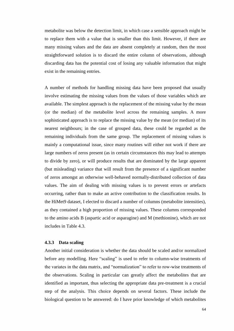
64
metabolite was below the detection limit, in which case a sensible approach might be
to replace them with a value that is smaller than this limit. However, if there are
many missing values and the data are absent completely at random, then the most
straightforward solution is to discard the entire column of observations, although
discarding data has the potential cost of losing any valuable information that might
exist in the remaining entries.
A number of methods for handling missing data have been proposed that usually
involve estimating the missing values from the values of those variables which are
available. The simplest approach is the replacement of the missing value by the mean
(or the median) of the metabolite level across the remaining samples. A more
sophisticated approach is to replace the missing value by the mean (or median) of its
nearest neighbours; in the case of grouped data, these could be regarded as the
remaining individuals from the same group. The replacement of missing values is
mainly a computational issue, since many routines will either not work if there are
large numbers of zeros present (as in certain circumstances this may lead to attempts
to divide by zero), or will produce results that are dominated by the large apparent
(but misleading) variance that will result from the presence of a significant number
of zeros amongst an otherwise well-behaved normally-distributed collection of data
values. The aim of dealing with missing values is to prevent errors or artefacts
occurring, rather than to make an active contribution to the classification results. In
the HiMet9 dataset, I elected to discard a number of columns (metabolite intensities),
as they contained a high proportion of missing values. These columns corresponded
to the amino acids B (aspartic acid or asparagine) and M (methionine), which are not
includes in Table 4.3.
4.3.3 Data scaling
Another initial consideration is whether the data should be scaled and/or normalized
before any modelling. Here “scaling” is used to refer to column-wise treatments of
the variates in the data matrix, and “normalization” to refer to row-wise treatments of
the observations. Scaling in particular can greatly affect the metabolites that are
identified as important, thus selecting the appropriate data pre-treatment is a crucial
step of the analysis. This choice depends on several factors. These include the
biological question to be answered: do I have prior knowledge of which metabolites
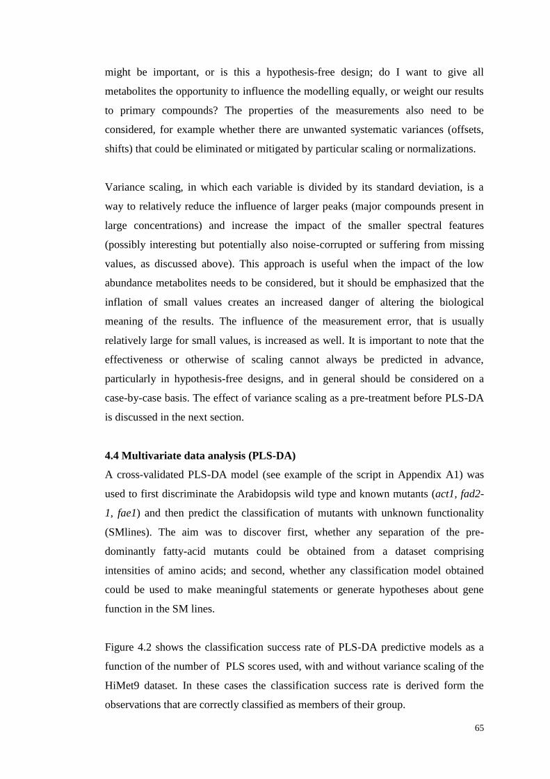
65
might be important, or is this a hypothesis-free design; do I want to give all
metabolites the opportunity to influence the modelling equally, or weight our results
to primary compounds? The properties of the measurements also need to be
considered, for example whether there are unwanted systematic variances (offsets,
shifts) that could be eliminated or mitigated by particular scaling or normalizations.
Variance scaling, in which each variable is divided by its standard deviation, is a
way to relatively reduce the influence of larger peaks (major compounds present in
large concentrations) and increase the impact of the smaller spectral features
(possibly interesting but potentially also noise-corrupted or suffering from missing
values, as discussed above). This approach is useful when the impact of the low
abundance metabolites needs to be considered, but it should be emphasized that the
inflation of small values creates an increased danger of altering the biological
meaning of the results. The influence of the measurement error, that is usually
relatively large for small values, is increased as well. It is important to note that the
effectiveness or otherwise of scaling cannot always be predicted in advance,
particularly in hypothesis-free designs, and in general should be considered on a
case-by-case basis. The effect of variance scaling as a pre-treatment before PLS-DA
is discussed in the next section.
4.4 Multivariate data analysis (PLS-DA)
A cross-validated PLS-DA model (see example of the script in Appendix A1) was
used to first discriminate the Arabidopsis wild type and known mutants (act1, fad2-
1, fae1) and then predict the classification of mutants with unknown functionality
(SMlines). The aim was to discover first, whether any separation of the pre-
dominantly fatty-acid mutants could be obtained from a dataset comprising
intensities of amino acids; and second, whether any classification model obtained
could be used to make meaningful statements or generate hypotheses about gene
function in the SM lines.
Figure 4.2 shows the classification success rate of PLS-DA predictive models as a
function of the number of PLS scores used, with and without variance scaling of the
HiMet9 dataset. In these cases the classification success rate is derived form the
observations that are correctly classified as members of their group.
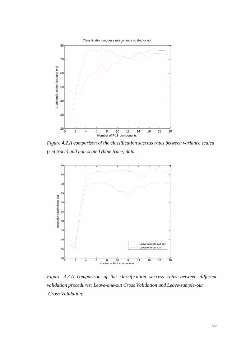
66
Figure 4.2.A comparison of the classification success rates between variance scaled
(red trace) and non-scaled (blue trace) data.
Figure 4.3.A comparison of the classification success rates between different
validation procedures; Leave-one-out Cross Validation and Leave-sample-out
Cross Validation.
0 2 4 6 8 10 12 14 16 18 2020
30
40
50
60
70
80
Classification success ratevariance scaled or not
Number of PLS components
Successfu
l cla
ssific
ations (
%)
0 2 4 6 8 10 12 14 16 18 2040
45
50
55
60
65
70
75
80
85
90Classification success rate for different cross validation segments
Number of PLS components
Successfu
l cla
ssific
ations (
%)
Leave-sample-out CV
Leave-one-out CV
67
The classification of the models themselves will be discussed below, but with
regards to pre-treatment, in this particular instance, variance-scaling compromises
the parsimony of the PLS-DA modelling. Amplifying the signals from the low
abundance metabolites (and their inherent noise) has made the task of obtaining an
effective model harder. Therefore, I henceforth employ mean-centering only as the
pre-treatment of choice in the present chapter.
4.4.1 Cross-validation design
Validation is a very important step in estimating the fit of a model to an independent
data set. In this thesis, PLS-DA models are evaluated using a cross-validation design.
The appropriate training/validation segmentation can be a crucial factor for
constructing robust predictive models (Broadhurst and Kell, 2006). In this section I
demonstrate an important parameter of the validation design related to the presence
of replicate measurements, and a potential pitfall, known as overfitting. In an overfit
model, the classification ability may superficially appear satisfactory, but in fact is
not statistically significant and the model is destined to perform less well when
validated on entirely new samples.
It is easy to highlight the numerical causes of gross overfitting by passing similarly
dimensioned sets of random numbers through the same modelling procedure
(Defernez and Kemsley, 1997). However, various more subtle forms of overfitting
can be manifested with real experimental data, often related to the idea of what
exactly constitutes an “independent” measurement. In the results shown on Figure
4.3, the dataset includes replicate measurements of each sample. In this case, leave-
one-out cross validation provides an ‘overoptimistic’ (overfit) result. The reason for
this behaviour is due to technical replicates tending to be classified together. Thus, as
the model dimensions increase as the training segment is fitted, the single validation
items follow suit and classify in the same way as their matching replicates in the
training segment, rather than providing an independent test of each dimensionality.
The cross-validation success rate is therefore unfairly augmented. In circumstances
such as this, only leave-sample-out cross-validation can reflect the true predictive
performance of the model. This demonstrates that the existence of technical
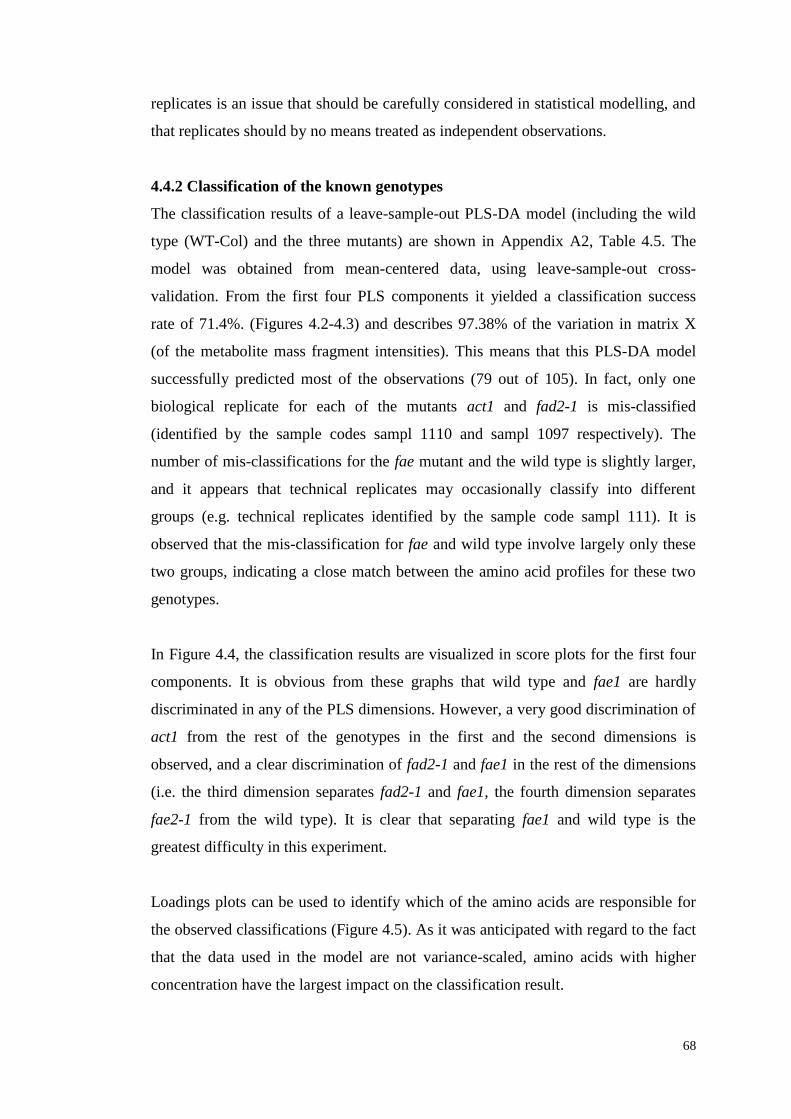
68
replicates is an issue that should be carefully considered in statistical modelling, and
that replicates should by no means treated as independent observations.
4.4.2 Classification of the known genotypes
The classification results of a leave-sample-out PLS-DA model (including the wild
type (WT-Col) and the three mutants) are shown in Appendix A2, Table 4.5. The
model was obtained from mean-centered data, using leave-sample-out cross-
validation. From the first four PLS components it yielded a classification success
rate of 71.4%. (Figures 4.2-4.3) and describes 97.38% of the variation in matrix X
(of the metabolite mass fragment intensities). This means that this PLS-DA model
successfully predicted most of the observations (79 out of 105). In fact, only one
biological replicate for each of the mutants act1 and fad2-1 is mis-classified
(identified by the sample codes sampl 1110 and sampl 1097 respectively). The
number of mis-classifications for the fae mutant and the wild type is slightly larger,
and it appears that technical replicates may occasionally classify into different
groups (e.g. technical replicates identified by the sample code sampl 111). It is
observed that the mis-classification for fae and wild type involve largely only these
two groups, indicating a close match between the amino acid profiles for these two
genotypes.
In Figure 4.4, the classification results are visualized in score plots for the first four
components. It is obvious from these graphs that wild type and fae1 are hardly
discriminated in any of the PLS dimensions. However, a very good discrimination of
act1 from the rest of the genotypes in the first and the second dimensions is
observed, and a clear discrimination of fad2-1 and fae1 in the rest of the dimensions
(i.e. the third dimension separates fad2-1 and fae1, the fourth dimension separates
fae2-1 from the wild type). It is clear that separating fae1 and wild type is the
greatest difficulty in this experiment.
Loadings plots can be used to identify which of the amino acids are responsible for
the observed classifications (Figure 4.5). As it was anticipated with regard to the fact
that the data used in the model are not variance-scaled, amino acids with higher
concentration have the largest impact on the classification result.

69
4.4.3 Predictions of the unknowns (SMlines)
The four-component PLS-DA model was used to classify the SMlines included in
HiMet9 experiment. The classification result is shown in Appendix A2, Table 4.6.
From a collection of 292 samples of SMlines, 231 samples were classified as wild
type, 45 samples were classified as fae1, only 15 samples were classified as act1 and
three samples as fad2-1. As can be seen, some of the biological and technical
replicates are assigned into two different groups. The reasons for such separation
could be the variability there is between biological replicates, as well as other
technical aspects (batch effects) that were not available in the metadata.
In order to enhance the interpretation of the classification result it is often useful to
draw graphs that show how the SMlines are scattered across the groups of known
mutants. In the Figures 4.6 to 4.9 the SMlines from each one of the groups are
superimposed on the classification result of the known mutants for the first two PLS
dimensions. Figure 4.6 shows the large amount of SMlines that were classified as
wild type, which seem to be largely superposed across the original fae1 group. This
is a reflection of the close similarity between these two types in the original
classification model. On Figure 4.7, it is very clear that the SMlines classified as
act1 are closer to the cluster of the act1 mutant, however, some of them are also very
close to the remaining groups. This is a reminder to exercise caution, and not to
interpret an act1 classification as entirely definitive.
Overall, the SMlines seem to be closely related to the wild type or the fae1 mutant,
however, considering that these two groups were the least well discriminated from
one another in the original model, it is very difficult to assign the SMlines with
absolute confidence to either of these groups and to come to firm conclusions about
gene functions.
4.5 Discussion on the limitations of the Himet9 work
In this work only one dataset from the HiMet9 experiment I presented, which was
kindly provided by Nigel Hardy of the University of Aberystwyth. However, during
the course of this study, the full Himet data was published in a paper focusing on the
application of machine learning (ML) to metabolomics data (Scott et al., 2010).
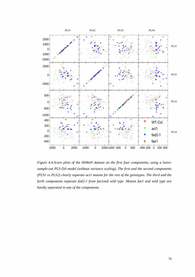
70
-400-200 0 200 400-1000 -500 0 500-2000 0 2000-2000 0 2000
-400
-200
0
200
400
-1000
-500
0
500
-2000
0
2000
-2000
-1000
0
1000
2000
Wt-col
act1
fad2-1
fae1
Figure 4.4.Score plots of the HiMet9 dataset on the first four components, using a leave-
sample-out PLS-DA model (without variance scaling). The first and the second components
(PLS1 vs PLS2) clearly separate act1 mutant for the rest of the genotypes. The third and the
forth components separate fad2-1 from fae1and wild type. Mutant fae1 and wild type are
hardly separated in any of the components.
PLS1
PLS1
PLS2
PLS2
PLS3 PLS4
PLS3
PLS4
WT-Col
act1
fad2-1
fae1
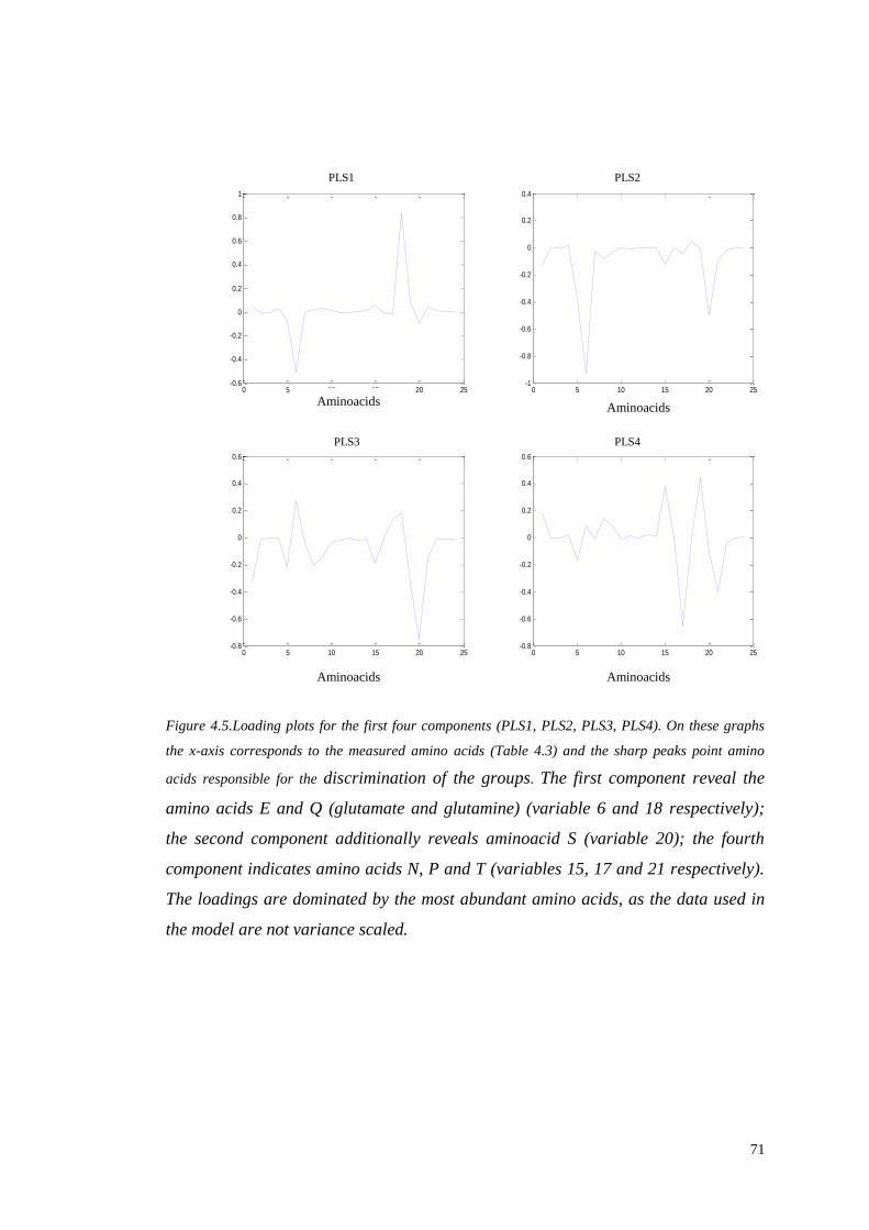
71
0 5 10 15 20 25-0.6
-0.4
-0.2
0
0.2
0.4
0.6
0.8
1LV1
0 5 10 15 20 25-1
-0.8
-0.6
-0.4
-0.2
0
0.2
0.4LV2
0 5 10 15 20 25-0.8
-0.6
-0.4
-0.2
0
0.2
0.4
0.6LV3
0 5 10 15 20 25-0.8
-0.6
-0.4
-0.2
0
0.2
0.4
0.6LV4
Figure 4.5.Loading plots for the first four components (PLS1, PLS2, PLS3, PLS4). On these graphs
the x-axis corresponds to the measured amino acids (Table 4.3) and the sharp peaks point amino
acids responsible for the discrimination of the groups. The first component reveal the
amino acids E and Q (glutamate and glutamine) (variable 6 and 18 respectively);
the second component additionally reveals aminoacid S (variable 20); the fourth
component indicates amino acids N, P and T (variables 15, 17 and 21 respectively).
The loadings are dominated by the most abundant amino acids, as the data used in
the model are not variance scaled.
PLS1 PLS2
PLS3 PLS4
Aminoacids
Aminoacids Aminoacids
Aminoacids
72
It was therefore considered that a more in depth analysis of Himet datasets was not
justified, and the use of this dataset was limited to demonstrating the application of
PLS-DA to classify known mutants and predict the classification of unknowns.
However, it is interesting that I have been able to distinguish mutants of lipid
metabolism (act1, fad2-1, fae1) solely on the basis of their amino acid profiles. This
conclusion is confirmed by Scott et al. (2010), who showed that all (apart from fad4
and tag1) mutants that were involved in HiMet experiments could be discriminated
by amino acid profiles. One might assume that they would more readily be separated
on the basis of carbohydrate or fatty acid profiles, but there is a close coupling of
carbon and nitrogen metabolism in plants (Stitt and Fernie, 2003). Metabolomics, for
example in potato tubers (Roessner et al, 2001) has been used previously to show
such a link and there are complex regulatory mechanisms known to ensure a balance
between carbon and nitrogen utilisation (Nunes-Nesi et al, 2010).
The incompleteness of the classification concerning the SMlines is partially due to
the small number of mutants included in this experiment. Any attempt to come to
conclusions regarding gene functions analysis would require the examination of
hundreds of mutants from different metabolic pathways. Moreover, a more
comprehensive collection of metadata could have helped the interpretation of the
mis-classifications of the SM-lines.
In summary, in this Chapter, I examined an LC-MS dataset of known metabolites
(24 amino acids; targeted metabolite analysis), where the peak detection and
deconvolution was performed manually, consequently the first (and last) steps of the
pipeline were not required. In the next Chapter, I will examine a complete GC-MS
untargeted metabolomics experiment, including hundreds of ions within a mass
range of 50-500 m/z representing known or structurally novel metabolites, which are
produced by pre-processing the raw data files using the XCMS software, and use
statistical modelling to make statements about the dataset that are of direct biological
interest.
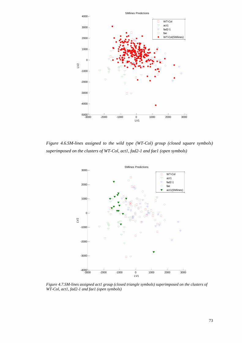
73
-3000 -2000 -1000 0 1000 2000 3000-4000
-3000
-2000
-1000
0
1000
2000
3000
LV1
LV
2
SMlines Predictions
WT-Col
act1
fad2-1
fae
act1(SMlines)
-3000 -2000 -1000 0 1000 2000 3000-5000
-4000
-3000
-2000
-1000
0
1000
2000
3000
4000
LV1
LV
2
SMlines Predictions
WT-Col
act1
fad2-1
fae
WT-Col(SMlines)
Figure 4.6.SM-lines assigned to the wild type (WT-Col) group (closed square symbols)
superimposed on the clusters of WT-Col, act1, fad2-1 and fae1 (open symbols)
Figure 4.7.SM-lines assigned act1 group (closed triangle symbols) superimposed on the clusters of
WT-Col, act1, fad2-1 and fae1 (open symbols)
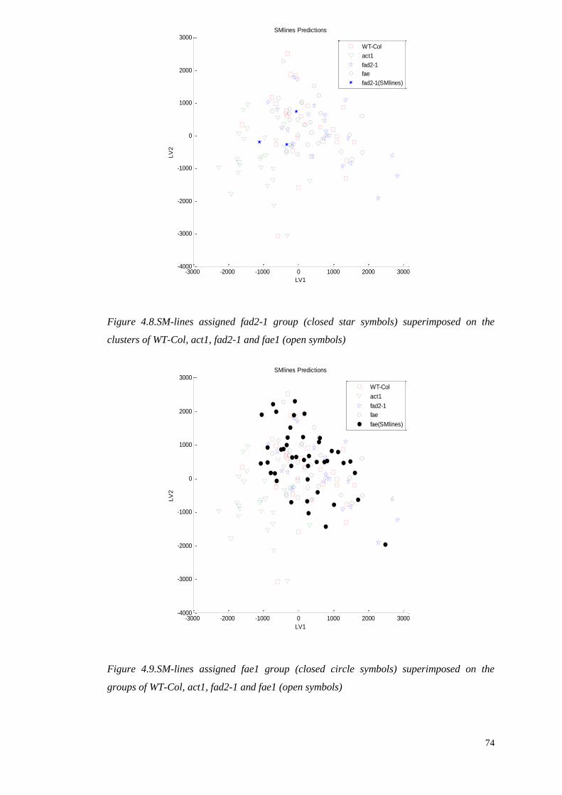
74
-3000 -2000 -1000 0 1000 2000 3000-4000
-3000
-2000
-1000
0
1000
2000
3000
LV1
LV
2
SMlines Predictions
WT-Col
act1
fad2-1
fae
fad2-1(SMlines)
-3000 -2000 -1000 0 1000 2000 3000-4000
-3000
-2000
-1000
0
1000
2000
3000
LV1
LV
2
SMlines Predictions
WT-Col
act1
fad2-1
fae
fae(SMlines)
Figure 4.8.SM-lines assigned fad2-1 group (closed star symbols) superimposed on the
clusters of WT-Col, act1, fad2-1 and fae1 (open symbols)
Figure 4.9.SM-lines assigned fae1 group (closed circle symbols) superimposed on the
groups of WT-Col, act1, fad2-1 and fae1 (open symbols)

75
CHAPTER 5:
A METABOLOMICS INVESTIGATION
OF STARCH METABOLISM
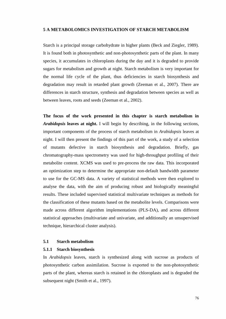
76
5 A METABOLOMICS INVESTIGATION OF STARCH METABOLISM
Starch is a principal storage carbohydrate in higher plants (Beck and Ziegler, 1989).
It is found both in photosynthetic and non-photosynthetic parts of the plant. In many
species, it accumulates in chloroplasts during the day and it is degraded to provide
sugars for metabolism and growth at night. Starch metabolism is very important for
the normal life cycle of the plant, thus deficiencies in starch biosynthesis and
degradation may result in retarded plant growth (Zeeman et al., 2007). There are
differences in starch structure, synthesis and degradation between species as well as
between leaves, roots and seeds (Zeeman et al., 2002).
The focus of the work presented in this chapter is starch metabolism in
Arabidopsis leaves at night. I will begin by describing, in the following sections,
important components of the process of starch metabolism in Arabidopsis leaves at
night. I will then present the findings of this part of the work, a study of a selection
of mutants defective in starch biosynthesis and degradation. Briefly, gas
chromatography-mass spectrometry was used for high-throughput profiling of their
metabolite content. XCMS was used to pre-process the raw data. This incorporated
an optimization step to determine the appropriate non-default bandwidth parameter
to use for the GC-MS data. A variety of statistical methods were then explored to
analyse the data, with the aim of producing robust and biologically meaningful
results. These included supervised statistical multivariate techniques as methods for
the classification of these mutants based on the metabolite levels. Comparisons were
made across different algorithm implementations (PLS-DA), and across different
statistical approaches (multivariate and univariate, and additionally an unsupervised
technique, hierarchical cluster analysis).
5.1 Starch metabolism
5.1.1 Starch biosynthesis
In Arabidopsis leaves, starch is synthesized along with sucrose as products of
photosynthetic carbon assimilation. Sucrose is exported to the non-photosynthetic
parts of the plant, whereas starch is retained in the chloroplasts and is degraded the
subsequent night (Smith et al., 1997).
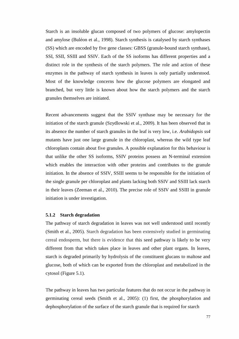
77
Starch is an insoluble glucan composed of two polymers of glucose: amylopectin
and amylose (Buléon et al., 1998). Starch synthesis is catalysed by starch synthases
(SS) which are encoded by five gene classes: GBSS (granule-bound starch synthase),
SSI, SSII, SSIII and SSIV. Each of the SS isoforms has different properties and a
distinct role in the synthesis of the starch polymers. The role and action of these
enzymes in the pathway of starch synthesis in leaves is only partially understood.
Most of the knowledge concerns how the glucose polymers are elongated and
branched, but very little is known about how the starch polymers and the starch
granules themselves are initiated.
Recent advancements suggest that the SSIV synthase may be necessary for the
initiation of the starch granule (Szydlowski et al., 2009). It has been observed that in
its absence the number of starch granules in the leaf is very low, i.e. Arabidopsis ss4
mutants have just one large granule in the chloroplast, whereas the wild type leaf
chloroplasts contain about five granules. A possible explanation for this behaviour is
that unlike the other SS isoforms, SSIV proteins possess an N-terminal extension
which enables the interaction with other proteins and contributes to the granule
initiation. In the absence of SSIV, SSIII seems to be responsible for the initiation of
the single granule per chloroplast and plants lacking both SSIV and SSIII lack starch
in their leaves (Zeeman et al., 2010). The precise role of SSIV and SSIII in granule
initiation is under investigation.
5.1.2 Starch degradation
The pathway of starch degradation in leaves was not well understood until recently
(Smith et al., 2005). Starch degradation has been extensively studied in germinating
cereal endosperm, but there is evidence that this seed pathway is likely to be very
different from that which takes place in leaves and other plant organs. In leaves,
starch is degraded primarily by hydrolysis of the constituent glucans to maltose and
glucose, both of which can be exported from the chloroplast and metabolized in the
cytosol (Figure 5.1).
The pathway in leaves has two particular features that do not occur in the pathway in
germinating cereal seeds (Smith et al., 2005): (1) first, the phosphorylation and
dephosphorylation of the surface of the starch granule that is required for starch
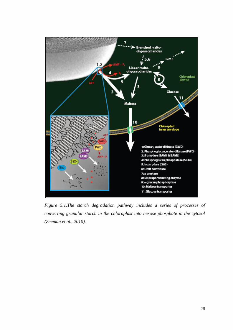
78
Figure 5.1.The starch degradation pathway includes a series of processes of
converting granular starch in the chloroplast into hexose phosphate in the cytosol
(Zeeman et al., 2010).
79
degradation (Yu et al., 2001), which involves the enzymes SEX1 (also known as
GWD1) and SEX4, (2) second, the export of maltose from the chloroplast and its
subsequent metabolism in the cytosol, which involves the maltose transporter protein
MEX1 and the transglucosidase DPE2 (Niittylä et al., 2004). Neither of these
features is yet fully understood, but it has been observed that mutations affecting the
above key proteins decrease starch breakdown, resulting in the accumulation of
starch over repeated diurnal cycles (Zeeman et al., 2010).
5.1.3 Phosphorylation and de-phosphorylation of the starch granule
The phosphorylation of the starch glucans is a process which serves to solubilise the
granule surface and allows the hydrolases access to the glucan chain. This process
requires a class of enzymes called glucan water dikinases (GWD). GWD has a high
affinity for crystalline malto-oligosaccharides, and phosphorylation results in
extensive solubilisation of the constituent oligosaccharide chains. Mutations that
eliminate the GWD protein or affect the dikinase domain of the enzyme dramatically
reduce the rate of starch degradation. Loss of GWD in Arabidopsis leaves (sex1
mutants) leads to a very severe starch-excess (sex) phenotype, accumulating amounts
of starch up to seven times greater than those in wild-type leaves (Yu et al., 2005). A
second enzyme, the phosphoglucan water kinase (PWD), is also required for normal
starch breakdown but the pwd mutants have a mild sex phenotype.
5.1.4 Fate of maltose
Maltose is produced by β-amylolysis inside the chloroplast, however none of the
enzymes that are capable of hydrolyzing maltose to produce glucose is plastidial.
There is strong evidence that maltose produced during starch degradation at night is
exported to the cytosol via a specific protein, MEX1, which is located in the inner
membrane of the chloroplast envelope. Mutations at the MEX1 locus cause
accumulation of both starch and maltose in Arabidopsis leaves. Maltose levels are at
least 40 times those of wild-type leaves (Chia et al., 2004).
In the cytosol, maltose is metabolized via a transglucosylation reaction. Extracts of
leaves lacking a predicted transglucosidase, DPE2, have a phenotype similar to that
of mex1 that lacks the maltose transporter. Maltose levels are many times higher than
80
those of normal plants and starch degradation is inhibited. The free glucose released
from the maltose is likely to be converted to hexose phosphate.
5.1.5 Pathway elucidation
The roles and importance of key enzymes in starch metabolism have been mainly
explored using two approaches: first, using forward genetics by selecting plants
unable to degrade starch from a mutant population, then finding which gene has been
mutated; second, using reverse genetics by obtaining mutants lacking expression of
genes from the genome that are predicted to encode enzymes that might be important
in starch degradation. In general, forward genetic Arabidopsis mutant studies have
been among the most successful approaches to revealing roles of genes and their
products, and elucidating biochemical, developmental and signalling pathways.
Forward genetics approaches have the advantage over reverse genetics that there is
no need for prior knowledge of the genes involved in the process; nevertheless it is
sometimes technically challenging to discover the gene responsible for a phenotype
by map-based cloning or discovery of the insertion element, as the selected
phenotypes may arise by secondary changes which may or may not be related to the
subject of study. Reverse genetics is also an excellent way to associate genes with
phenotypes, though a large number of mutants with a wide range of phenotypic
assays is required for producing detectable phenotypes. Ultimately, both of these
methods are time consuming, thus restricting the rate of discovery of gene function.
A more rapid way to gain information about the functions of important enzymes is to
use metabolomics as a functional genomics tool in order to explore what happens
to the metabolism when they are lost, and to compare the effects of loss of different
components of the pathway. Metabolite profiling is potentially a valuable method for
these comparisons, because it enables a large number of metabolites to be analysed
simultaneously and gives a broad view of metabolism. However, in order to gain
meaningful information from very complex metabolite profiles, which would allow
the effective preliminary characterization of classical genetic mutants, it is necessary
to compare large metabolomic datasets, and to use robust statistical methods to make
these comparisons.
81
5.2 Materials and methods
5.2.1 Mutants selection
Five mutants deficient in starch metabolism were used to determine the effect of loss
of different proteins on the metabolite profile of Arabidopsis leaves. The collection
of mutants includes one mutant deficient in starch biosynthesis, ss4, and four
mutants deficient in starch degradation: sex1 and sex4 (involved with the
phosphorylation and dephosphorylation of the starch granule) and mex1 and dpe2
(involved with the maltose metabolism). All mutants used were of Columbia (Col-0)
ecotype background. Wild type plants (Col-0) were used for comparisons. In Table
5.1 I list the replicates (seven for each genotype) and the day on which the GC-MS
analysis was performed. The latter will be discussed as an important consideration
during the data analysis.
5.2.2 Plant growth
Arabidopsis (Arabidopsis thaliana) ecotypes Col-0 and their mutants were grown in
a climate-controlled chamber set to growth conditions comprising cycles of 12 hours
light at 20°C followed by 12 hours dark at 16°C. Relative humidity was kept
between 60 and 75%. Plants of each genotype were randomized with respect to
position within the growth chamber shelving. Mature rosette stage, pre-flowering
specimens were harvested 1 hour before the end of the dark period (Boyes et al.,
2001) and immediately frozen in liquid nitrogen.
5.2.3 Extraction and GC-MS analyses of Arabidopsis leaf metabolites
The extraction and the analysis were performed by Baldeep Kular (JIC) and Lionel
Hill (JIC), respectively. The extraction method was based on that described by
Roessner et al.(2000 & 2001). Leaves were ground to a powder while frozen in
liquid nitrogen using a mortar and pestle and then freeze-dried and stored at -80°C
until needed. For soluble metabolite profiling by GC-MS analysis, leaf material (40–
60 mg) was extracted in 2 ml of 100% methanol together with an internal standard
(0.050 mg/ml phenyl-α-D-glucopyranoside, Sigma P6626; Sigma-Aldrich
Corporation, St. Louis, Missouri, USA). The mixture was heated and sonicated in a
screw-capped glass tube at 80°C for 15 minutes. Insoluble material was removed by
centrifugation. The samples were then evaporated to dryness under vacuum at 40°C.
Samples were dissolved in 100 μl of 2% methoxyamine hydrochloride (Aldrich,
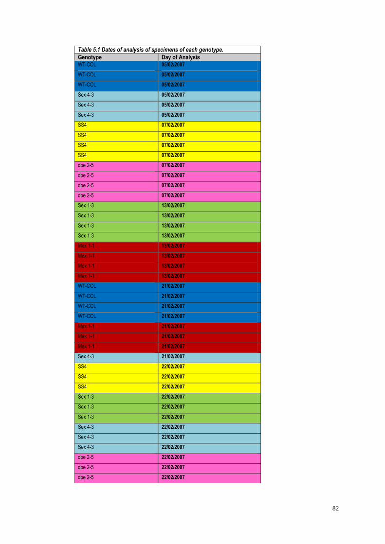
82
Table 5.1 Dates of analysis of specimens of each genotype.
Genotype Day of Analysis WT-COL 05/02/2007
WT-COL 05/02/2007
WT-COL 05/02/2007
Sex 4-3 05/02/2007
Sex 4-3 05/02/2007
Sex 4-3 05/02/2007
SS4 07/02/2007
SS4 07/02/2007
SS4 07/02/2007
SS4 07/02/2007
dpe 2-5 07/02/2007
dpe 2-5 07/02/2007
dpe 2-5 07/02/2007
dpe 2-5 07/02/2007
Sex 1-3 13/02/2007
Sex 1-3 13/02/2007
Sex 1-3 13/02/2007
Sex 1-3 13/02/2007
Mex 1-1 13/02/2007
Mex 1-1 13/02/2007
Mex 1-1 13/02/2007
Mex 1-1 13/02/2007
WT-COL 21/02/2007
WT-COL 21/02/2007
WT-COL 21/02/2007
WT-COL 21/02/2007
Mex 1-1 21/02/2007
Mex 1-1 21/02/2007
Mex 1-1 21/02/2007
Sex 4-3 21/02/2007
SS4 22/02/2007
SS4 22/02/2007
SS4 22/02/2007
Sex 1-3 22/02/2007
Sex 1-3 22/02/2007
Sex 1-3 22/02/2007
Sex 4-3 22/02/2007
Sex 4-3 22/02/2007
Sex 4-3 22/02/2007
dpe 2-5 22/02/2007
dpe 2-5 22/02/2007
dpe 2-5 22/02/2007
83
22,690-4; Sigma-Aldrich Corporation, St. Louis, Missouri, USA) in pyridine for 90
minutes at 30°C with constant stirring to protect the carbonyl moieties. The samples
were then silylated with the addition of 100 μl of MSTFA (N-methyl-N-
[trimethylsil] trifluoroacetamide, Pierce Biotechnology, now Thermo Scientific,
Rockford, Illinois, USA) for 30 minutes at 37°C with constant stirring. The samples
were transferred to glass GC vials and left for 2 hours before analysis.
The analyses was performed using (Agilent Technologies, Wilmington, Delaware,
USA) GC 6890N coupled to a Mass Selective Detector 5973inert. Automated
splitless injections (1 μl) were made using an Agilent 7683 automatic sampler.
Conditions of chromatography were: inlet temperature 250oC; the carrier gas was
helium at a constant flow rate of 0.9ml/min; nominal inlet pressure of 7.86 psi. The
oven temperature program was: 80oC for 2 minutes, 10
oC/min to 340
oC then held for
7 minutes, giving a total run time of 35 minutes. The column was a ZB-5HT Inferno
(Zebron: 7HG-G015-02, Phenomenex, Macclesfield, UK.) 30m x 0.25mm x 0.25 μm
with a 5 meter guard column incorporated on the front end. The mass spectrometer
parameters were: using electron ionisation in positive mode (70eV), with a source
temperature of 230oC and a quad temperature of 150
oC, according to the
manufacturer’s defaults. Total ion scans were made from 50 to 500 amu and all data
was processed via the Agilent GC Chemstation software (D.01.00) in conjunction
with the NIST Mass Spectral Library, V2.0 (National Institute of Standards and
Technology, Gaithersburg, Maryland, USA) and the Gölm Metabolome database
(http://csbdb.mpimp-golm.mpg.de/csbdb/gmd/msri/gmd_msri.html) hosted at the
Max Planck Institute of Molecular Plant Physiology, Potsdam, Germany.
5.3 Results and discussion
5.3.1 Visual examination of metabolite profiles
The composition of individuals of each genotype can be broadly visualized by
displaying their metabolite profiles as annotated chromatograms. Figure 5.2 shows
an illustrative comparison between all metabolite profiles of the wild type and
mutant plants. Variations in metabolite levels in comparison to the wild type can
reveal distinct patterns of change affecting central metabolism in each genotype.
Nevertheless, it should be taken into consideration that firstly, the samples are a
“snapshot” taken at a single time point, and secondly, a visual point-by-point
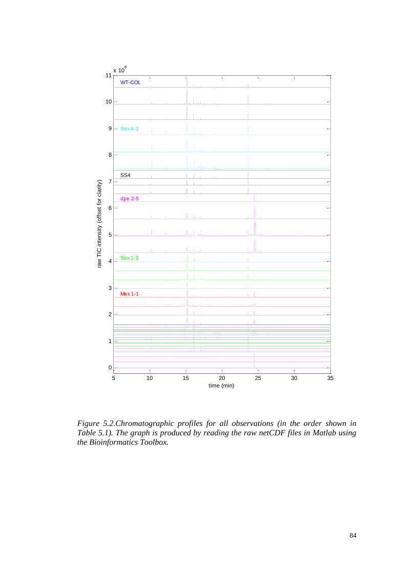
84
Figure 5.2.Chromatographic profiles for all observations (in the order shown in
Table 5.1). The graph is produced by reading the raw netCDF files in Matlab using
the Bioinformatics Toolbox.
5 10 15 20 25 30 35
0
1
2
3
4
5
6
7
8
9
10
11x 10
8
Mex 1-1
Sex 1-3
dpe 2-5
SS4
Sex 4-3
WT-COL
time (min)
raw
TIC
inte
nsity (
off
set
for
cla
rity
)
85
analysis is not practical on the metabolomic scale. Furthermore, there is a substantial
within-genotype variance, which is a clear indication of the need for data
normalization, discussed further below.
The peaks in the chromatogram were identified by using the Golm Metabolome
Database (http://csbdb.mpimp-golm.mpg.de/csbdb/gmd/msri/gmd_msri.html)
through the NIST software. Over 100 metabolites were detected in each sample.
These included a range of chemical classes, mainly represented by sugars, sugar
alcohols, amino acids and organic acids.
5.3.2 Data pre-processing
XCMS software (version 2.10.1) was used to deconvolute and align mass ions from
the 42 data files (samples) into a single data set. The input files were in NetCDF
format, created by format conversion of the raw GC-MS datafiles.
As discussed in Chapter 3, the default XCMS parameters are by default intended for
pre-processing LC-MS data. Historically, XCMS has largely been used for
processing this type of data. However, modifications are required for handling GC-
MS data, arising from a substantive difference in the width of the chromatographic
peaks, which are much wider for LC-MS data. Specifically, the XCMS parameters
(see section 3.1.3) which require new values are: fwhm (full-width half-maximum;
xcmsSet function) and bw (band width; group function). Failure to adjust these
parameters appropriately will lead to XCMS overlooking a large proportion of the
peaks/compounds present in the data.
In Figure 5.3 it is shown how the fwhm parameter was optimized for the specific
GC-MS dataset. On the basis of this, it was determined that the value for this
parameter for handling GC-MS data should be set to 3 (a substantial change,
compared with the LC-MS default of 30). The bandwidth parameter bw was set to
10. (Full details of the various XCMS parameters and pre-processing steps were
discussed in Chapter 3, where a typical chromatographic peak of this dataset and the
band width as a grouping variable are shown in Figures 3.3 and 3.4, respectively.)
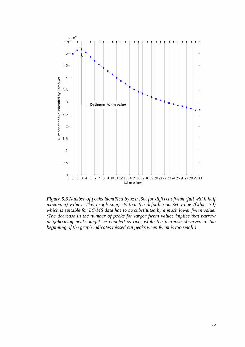
86
Figure 5.3.Number of peaks identified by xcmsSet for different fwhm (full width half
maximum) values. This graph suggests that the default xcmsSet value (fwhm=30)
which is suitable for LC-MS data has to be substituted by a much lower fwhm value.
(The decrease in the number of peaks for larger fwhm values implies that narrow
neighbouring peaks might be counted as one, while the increase observed in the
beginning of the graph indicates missed out peaks when fwhm is too small.)
0 1 2 3 4 5 6 7 8 9 10 1112 1314 151617 1819 202122 2324 252627 2829 300
0.5
1
1.5
2
2.5
3
3.5
4
4.5
5
5.5x 10
4
fwhm values
Num
ber
of
peaks indentifid b
y x
cm
sS
et
Optimum fwhm value
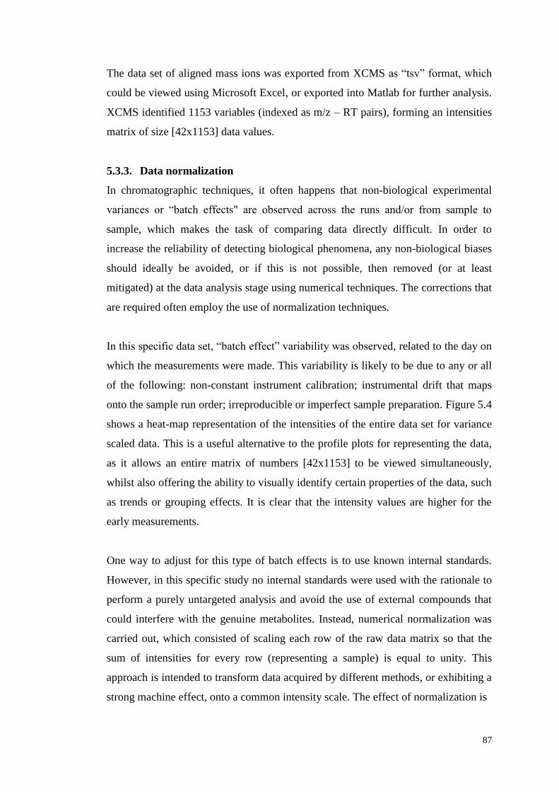
87
The data set of aligned mass ions was exported from XCMS as “tsv” format, which
could be viewed using Microsoft Excel, or exported into Matlab for further analysis.
XCMS identified 1153 variables (indexed as m/z – RT pairs), forming an intensities
matrix of size [42x1153] data values.
5.3.3. Data normalization
In chromatographic techniques, it often happens that non-biological experimental
variances or “batch effects" are observed across the runs and/or from sample to
sample, which makes the task of comparing data directly difficult. In order to
increase the reliability of detecting biological phenomena, any non-biological biases
should ideally be avoided, or if this is not possible, then removed (or at least
mitigated) at the data analysis stage using numerical techniques. The corrections that
are required often employ the use of normalization techniques.
In this specific data set, “batch effect” variability was observed, related to the day on
which the measurements were made. This variability is likely to be due to any or all
of the following: non-constant instrument calibration; instrumental drift that maps
onto the sample run order; irreproducible or imperfect sample preparation. Figure 5.4
shows a heat-map representation of the intensities of the entire data set for variance
scaled data. This is a useful alternative to the profile plots for representing the data,
as it allows an entire matrix of numbers [42x1153] to be viewed simultaneously,
whilst also offering the ability to visually identify certain properties of the data, such
as trends or grouping effects. It is clear that the intensity values are higher for the
early measurements.
One way to adjust for this type of batch effects is to use known internal standards.
However, in this specific study no internal standards were used with the rationale to
perform a purely untargeted analysis and avoid the use of external compounds that
could interfere with the genuine metabolites. Instead, numerical normalization was
carried out, which consisted of scaling each row of the raw data matrix so that the
sum of intensities for every row (representing a sample) is equal to unity. This
approach is intended to transform data acquired by different methods, or exhibiting a
strong machine effect, onto a common intensity scale. The effect of normalization is
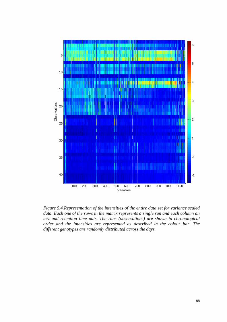
88
Figure 5.4.Representation of the intensities of the entire data set for variance scaled
data. Each one of the rows in the matrix represents a single run and each column an
m/z and retention time pair. The runs (observations) are shown in chronological
order and the intensities are represented as described in the colour bar. The
different genotypes are randomly distributed across the days.
Variables
Observ
ations
100 200 300 400 500 600 700 800 900 1000 1100
5
10
15
20
25
30
35
40 -1
0
1
2
3
4
5
6
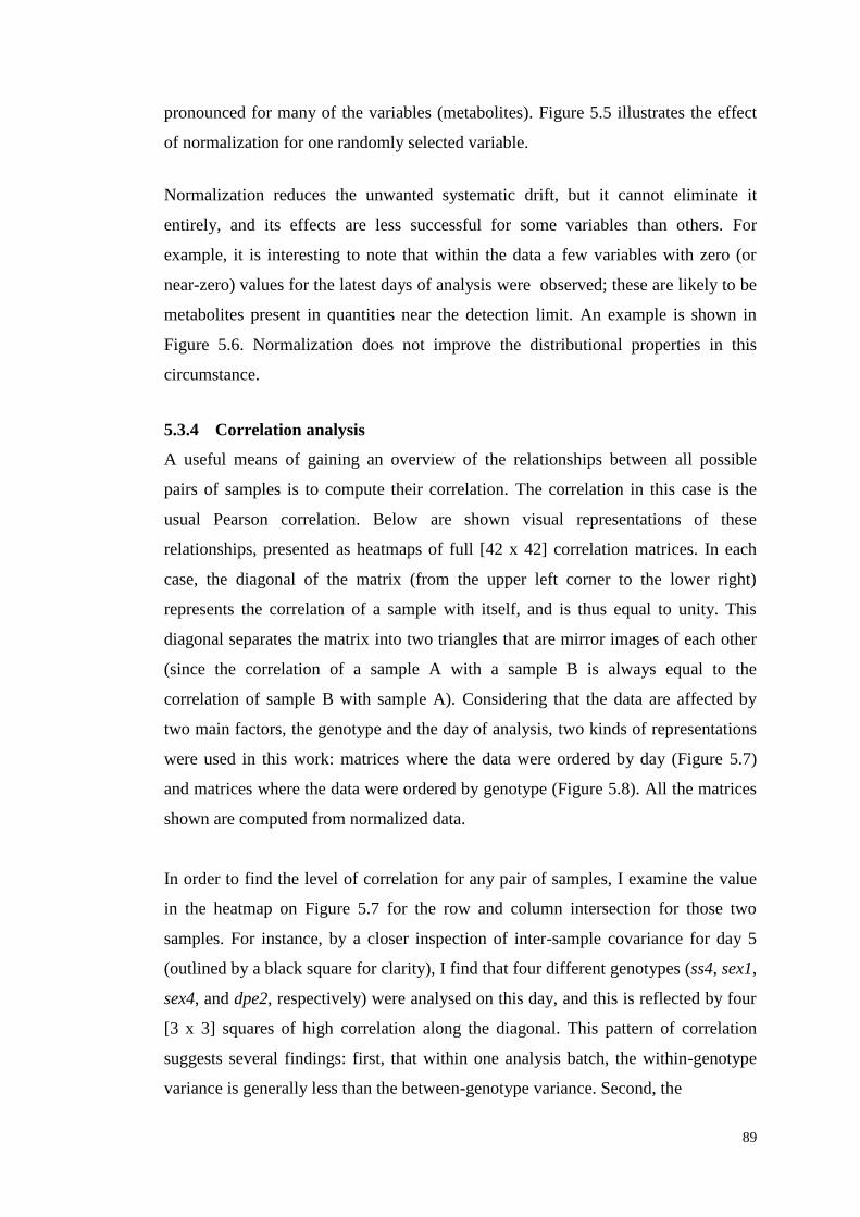
89
pronounced for many of the variables (metabolites). Figure 5.5 illustrates the effect
of normalization for one randomly selected variable.
Normalization reduces the unwanted systematic drift, but it cannot eliminate it
entirely, and its effects are less successful for some variables than others. For
example, it is interesting to note that within the data a few variables with zero (or
near-zero) values for the latest days of analysis were observed; these are likely to be
metabolites present in quantities near the detection limit. An example is shown in
Figure 5.6. Normalization does not improve the distributional properties in this
circumstance.
5.3.4 Correlation analysis
A useful means of gaining an overview of the relationships between all possible
pairs of samples is to compute their correlation. The correlation in this case is the
usual Pearson correlation. Below are shown visual representations of these
relationships, presented as heatmaps of full [42 x 42] correlation matrices. In each
case, the diagonal of the matrix (from the upper left corner to the lower right)
represents the correlation of a sample with itself, and is thus equal to unity. This
diagonal separates the matrix into two triangles that are mirror images of each other
(since the correlation of a sample A with a sample B is always equal to the
correlation of sample B with sample A). Considering that the data are affected by
two main factors, the genotype and the day of analysis, two kinds of representations
were used in this work: matrices where the data were ordered by day (Figure 5.7)
and matrices where the data were ordered by genotype (Figure 5.8). All the matrices
shown are computed from normalized data.
In order to find the level of correlation for any pair of samples, I examine the value
in the heatmap on Figure 5.7 for the row and column intersection for those two
samples. For instance, by a closer inspection of inter-sample covariance for day 5
(outlined by a black square for clarity), I find that four different genotypes (ss4, sex1,
sex4, and dpe2, respectively) were analysed on this day, and this is reflected by four
[3 x 3] squares of high correlation along the diagonal. This pattern of correlation
suggests several findings: first, that within one analysis batch, the within-genotype
variance is generally less than the between-genotype variance. Second, the
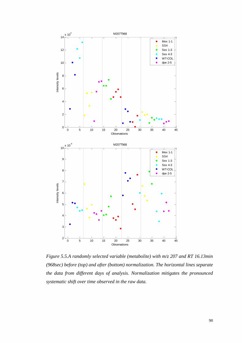
90
Figure 5.5.A randomly selected variable (metabolite) with m/z 207 and RT 16.13min
(968sec) before (top) and after (bottom) normalization. The horizontal lines separate
the data from different days of analysis. Normalization mitigates the pronounced
systematic shift over time observed in the raw data.
0 5 10 15 20 25 30 35 40 450
2
4
6
8
10
12
14x 10
4
Observations
Inte
nsity levels
M207T968
Mex 1-1
SS4
Sex 1-3
Sex 4-3
WT-COL
dpe 2-5
0 5 10 15 20 25 30 35 40 452
3
4
5
6
7
8
9
10x 10
-4
Observations
Inte
nsity levels
M207T968
Mex 1-1
SS4
Sex 1-3
Sex 4-3
WT-COL
dpe 2-5
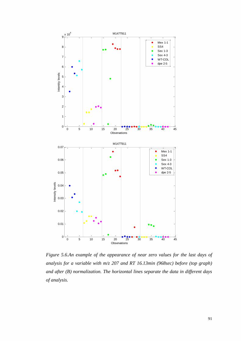
91
Figure 5.6.An example of the appearance of near zero values for the last days of
analysis for a variable with m/z 207 and RT 16.13min (968sec) before (top graph)
and after (B) normalization. The horizontal lines separate the data in different days
of analysis.
0 5 10 15 20 25 30 35 40 450
1
2
3
4
5
6
7
8
9x 10
6 M147T911
Observations
Inte
ntity
levels
Mex 1-1
SS4
Sex 1-3
Sex 4-3
WT-COL
dpe 2-5
0 5 10 15 20 25 30 35 40 450
0.01
0.02
0.03
0.04
0.05
0.06
0.07
Observations
Inte
nsity levels
M147T911
Mex 1-1
SS4
Sex 1-3
Sex 4-3
WT-COL
dpe 2-5
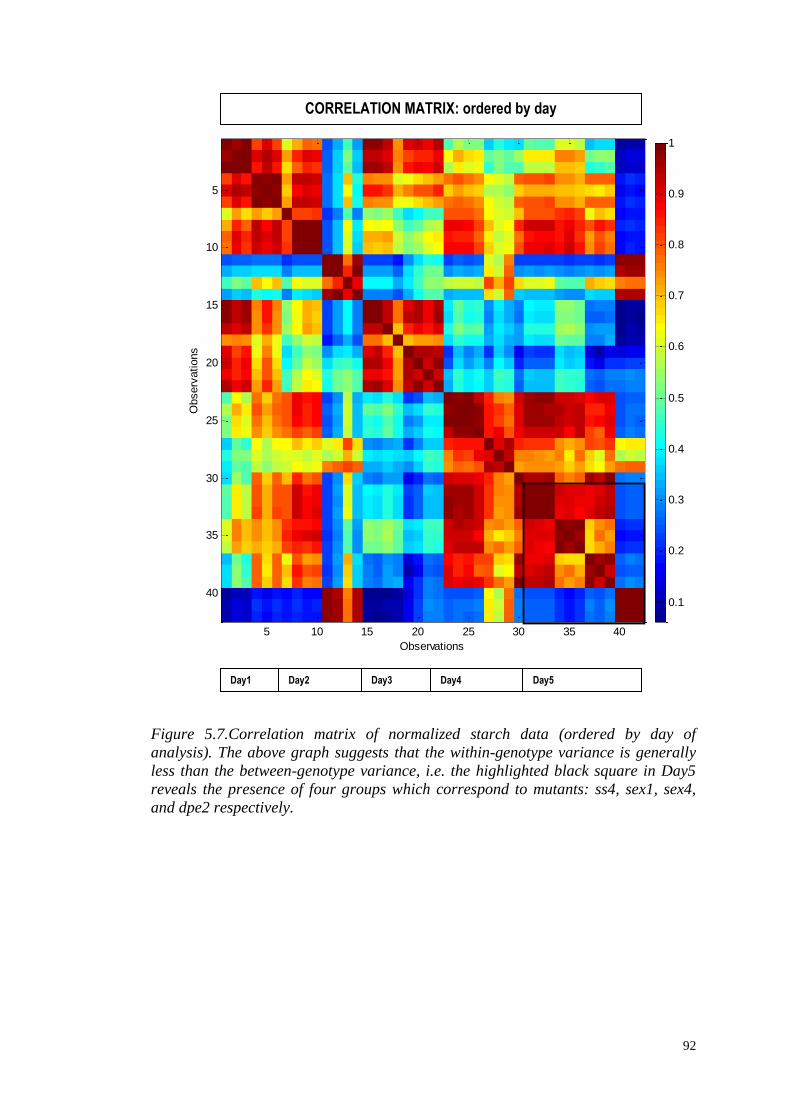
92
Figure 5.7.Correlation matrix of normalized starch data (ordered by day of
analysis). The above graph suggests that the within-genotype variance is generally
less than the between-genotype variance, i.e. the highlighted black square in Day5
reveals the presence of four groups which correspond to mutants: ss4, sex1, sex4,
and dpe2 respectively.
Observations
Observ
ations
5 10 15 20 25 30 35 40
5
10
15
20
25
30
35
400.1
0.2
0.3
0.4
0.5
0.6
0.7
0.8
0.9
1
CORRELATION MATRIX: ordered by day
Day1 Day2 Day3 Day4 Day5
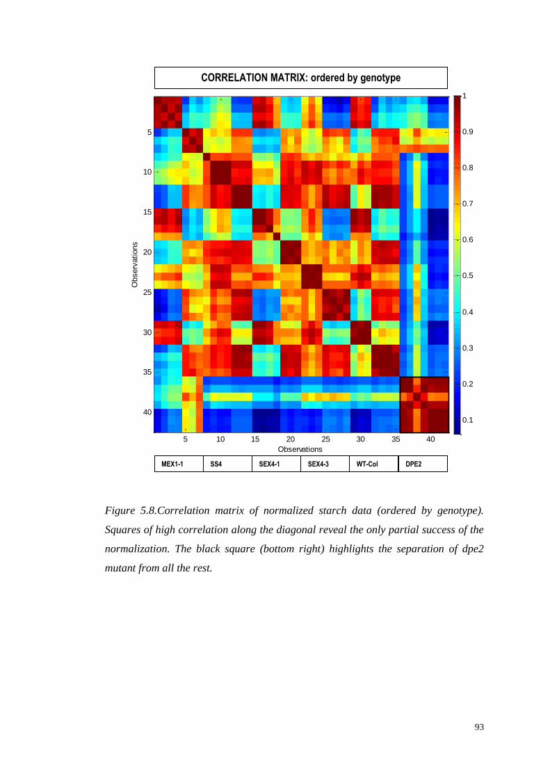
93
Figure 5.8.Correlation matrix of normalized starch data (ordered by genotype).
Squares of high correlation along the diagonal reveal the only partial success of the
normalization. The black square (bottom right) highlights the separation of dpe2
mutant from all the rest.
Observations
Observ
ations
5 10 15 20 25 30 35 40
5
10
15
20
25
30
35
400.1
0.2
0.3
0.4
0.5
0.6
0.7
0.8
0.9
1
CORRELATION MATRIX: ordered by genotype
MEX1-1 SS4 SEX4-1 SEX4-3 WT-Col DPE2
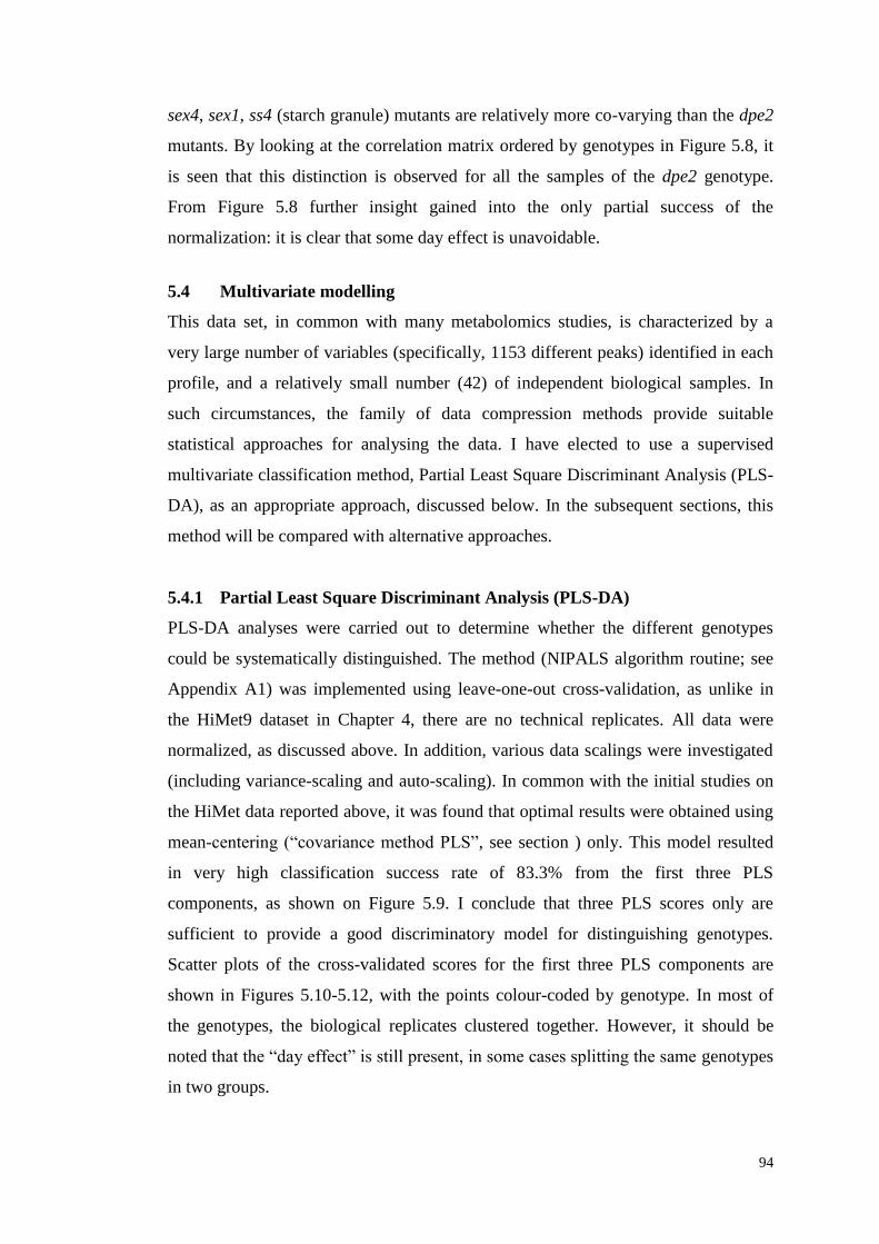
94
sex4, sex1, ss4 (starch granule) mutants are relatively more co-varying than the dpe2
mutants. By looking at the correlation matrix ordered by genotypes in Figure 5.8, it
is seen that this distinction is observed for all the samples of the dpe2 genotype.
From Figure 5.8 further insight gained into the only partial success of the
normalization: it is clear that some day effect is unavoidable.
5.4 Multivariate modelling
This data set, in common with many metabolomics studies, is characterized by a
very large number of variables (specifically, 1153 different peaks) identified in each
profile, and a relatively small number (42) of independent biological samples. In
such circumstances, the family of data compression methods provide suitable
statistical approaches for analysing the data. I have elected to use a supervised
multivariate classification method, Partial Least Square Discriminant Analysis (PLS-
DA), as an appropriate approach, discussed below. In the subsequent sections, this
method will be compared with alternative approaches.
5.4.1 Partial Least Square Discriminant Analysis (PLS-DA)
PLS-DA analyses were carried out to determine whether the different genotypes
could be systematically distinguished. The method (NIPALS algorithm routine; see
Appendix A1) was implemented using leave-one-out cross-validation, as unlike in
the HiMet9 dataset in Chapter 4, there are no technical replicates. All data were
normalized, as discussed above. In addition, various data scalings were investigated
(including variance-scaling and auto-scaling). In common with the initial studies on
the HiMet data reported above, it was found that optimal results were obtained using
mean-centering (“covariance method PLS”, see section ) only. This model resulted
in very high classification success rate of 83.3% from the first three PLS
components, as shown on Figure 5.9. I conclude that three PLS scores only are
sufficient to provide a good discriminatory model for distinguishing genotypes.
Scatter plots of the cross-validated scores for the first three PLS components are
shown in Figures 5.10-5.12, with the points colour-coded by genotype. In most of
the genotypes, the biological replicates clustered together. However, it should be
noted that the “day effect” is still present, in some cases splitting the same genotypes
in two groups.
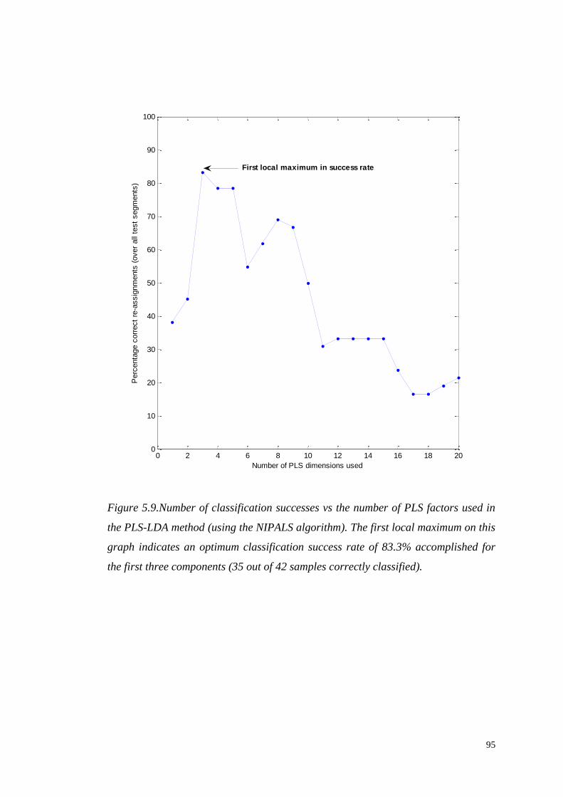
95
Figure 5.9.Number of classification successes vs the number of PLS factors used in
the PLS-LDA method (using the NIPALS algorithm). The first local maximum on this
graph indicates an optimum classification success rate of 83.3% accomplished for
the first three components (35 out of 42 samples correctly classified).
0 2 4 6 8 10 12 14 16 18 200
10
20
30
40
50
60
70
80
90
100
Number of PLS dimensions used
Perc
enta
ge c
orr
ect
re-a
ssig
nm
ents
(over
all
test
segm
ents
)
First local maximum in success rate
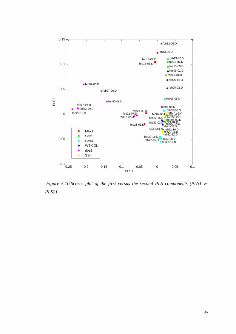
96
Figure 5.10.Scores plot of the first versus the second PLS components (PLS1 vs
PLS2).
-0.25 -0.2 -0.15 -0.1 -0.05 0 0.05 0.1-0.1
-0.05
0
0.05
0.1
0.15
PLS1
PLS
2
feb05-01.D
feb05-02.D
feb05-03.D
feb05-04.D
feb05-05.D
feb05-06.D
feb07-01.D
feb07-02.D
feb07-03.D feb07-04.D
feb07-05.D
feb07-06.D
feb07-07.D
feb07-08.D
feb13-01.D
feb13-02.D
feb13-03.D
feb13-04.D
feb13-05.D
feb13-06.D
feb13-07.D
feb13-08.D
feb21-01.D
feb21-02.D
feb21-03.D
feb21-04.Dfeb21-05.D
feb21-06.Dfeb21-07.D
feb21-08.D
feb22-10.Dfeb22-11.Dfeb22-12.D
feb22-13.D
feb22-14.D
feb22-15.D
feb22-16.Dfeb22-17.D
feb22-18.D
feb22-19.D
feb22-20.D
feb22-21.D
Mex1
Sex1
Sex4
WT-COL
dpe2
SS4
97
Figure 5.11.Scores plot of the first versus the third PLS components (PLS1 vs PLS3).
-0.25 -0.2 -0.15 -0.1 -0.05 0 0.05 0.1-0.06
-0.05
-0.04
-0.03
-0.02
-0.01
0
0.01
0.02
0.03
0.04
PLS1
PLS
3
feb05-01.D
feb05-02.D
feb05-03.D
feb05-04.D
feb05-05.D
feb05-06.D
feb07-01.D
feb07-02.D
feb07-03.D
feb07-04.D
feb07-05.D
feb07-06.D
feb07-07.D
feb07-08.D
feb13-01.Dfeb13-02.D
feb13-03.Dfeb13-04.D
feb13-05.D
feb13-06.D
feb13-07.D
feb13-08.D
feb21-01.Dfeb21-02.D
feb21-03.Dfeb21-04.D
feb21-05.D
feb21-06.D
feb21-07.D
feb21-08.D
feb22-10.Dfeb22-11.D
feb22-12.D
feb22-13.D
feb22-14.D
feb22-15.D
feb22-16.D
feb22-17.Dfeb22-18.D
feb22-19.D
feb22-20.D
feb22-21.D
Mex1
SS4
Sex1
Sex4
WT-COL
dpe2
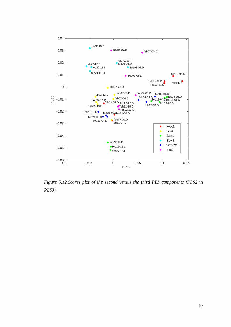
98
Figure 5.12.Scores plot of the second versus the third PLS components (PLS2 vs
PLS3).
-0.1 -0.05 0 0.05 0.1 0.15-0.06
-0.05
-0.04
-0.03
-0.02
-0.01
0
0.01
0.02
0.03
0.04
PLS2
PLS
3
feb05-01.D
feb05-02.D
feb05-03.D
feb05-04.D
feb05-05.D
feb05-06.D
feb07-01.D
feb07-02.D
feb07-03.D
feb07-04.D
feb07-05.D
feb07-06.D
feb07-07.D
feb07-08.D
feb13-01.Dfeb13-02.D
feb13-03.D
feb13-04.D
feb13-05.D
feb13-06.D
feb13-07.D
feb13-08.D
feb21-01.D feb21-02.D
feb21-03.D
feb21-04.D
feb21-05.D
feb21-06.D
feb21-07.D
feb21-08.D
feb22-10.D
feb22-11.D
feb22-12.D
feb22-13.D
feb22-14.D
feb22-15.D
feb22-16.D
feb22-17.D
feb22-18.D
feb22-19.D
feb22-20.D
feb22-21.D
Mex1
SS4
Sex1
Sex4
WT-COL
dpe2
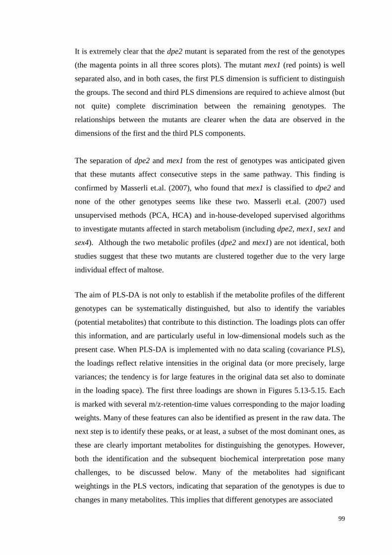
99
It is extremely clear that the dpe2 mutant is separated from the rest of the genotypes
(the magenta points in all three scores plots). The mutant mex1 (red points) is well
separated also, and in both cases, the first PLS dimension is sufficient to distinguish
the groups. The second and third PLS dimensions are required to achieve almost (but
not quite) complete discrimination between the remaining genotypes. The
relationships between the mutants are clearer when the data are observed in the
dimensions of the first and the third PLS components.
The separation of dpe2 and mex1 from the rest of genotypes was anticipated given
that these mutants affect consecutive steps in the same pathway. This finding is
confirmed by Masserli et.al. (2007), who found that mex1 is classified to dpe2 and
none of the other genotypes seems like these two. Masserli et.al. (2007) used
unsupervised methods (PCA, HCA) and in-house-developed supervised algorithms
to investigate mutants affected in starch metabolism (including dpe2, mex1, sex1 and
sex4). Although the two metabolic profiles (dpe2 and mex1) are not identical, both
studies suggest that these two mutants are clustered together due to the very large
individual effect of maltose.
The aim of PLS-DA is not only to establish if the metabolite profiles of the different
genotypes can be systematically distinguished, but also to identify the variables
(potential metabolites) that contribute to this distinction. The loadings plots can offer
this information, and are particularly useful in low-dimensional models such as the
present case. When PLS-DA is implemented with no data scaling (covariance PLS),
the loadings reflect relative intensities in the original data (or more precisely, large
variances; the tendency is for large features in the original data set also to dominate
in the loading space). The first three loadings are shown in Figures 5.13-5.15. Each
is marked with several m/z-retention-time values corresponding to the major loading
weights. Many of these features can also be identified as present in the raw data. The
next step is to identify these peaks, or at least, a subset of the most dominant ones, as
these are clearly important metabolites for distinguishing the genotypes. However,
both the identification and the subsequent biochemical interpretation pose many
challenges, to be discussed below. Many of the metabolites had significant
weightings in the PLS vectors, indicating that separation of the genotypes is due to
changes in many metabolites. This implies that different genotypes are associated
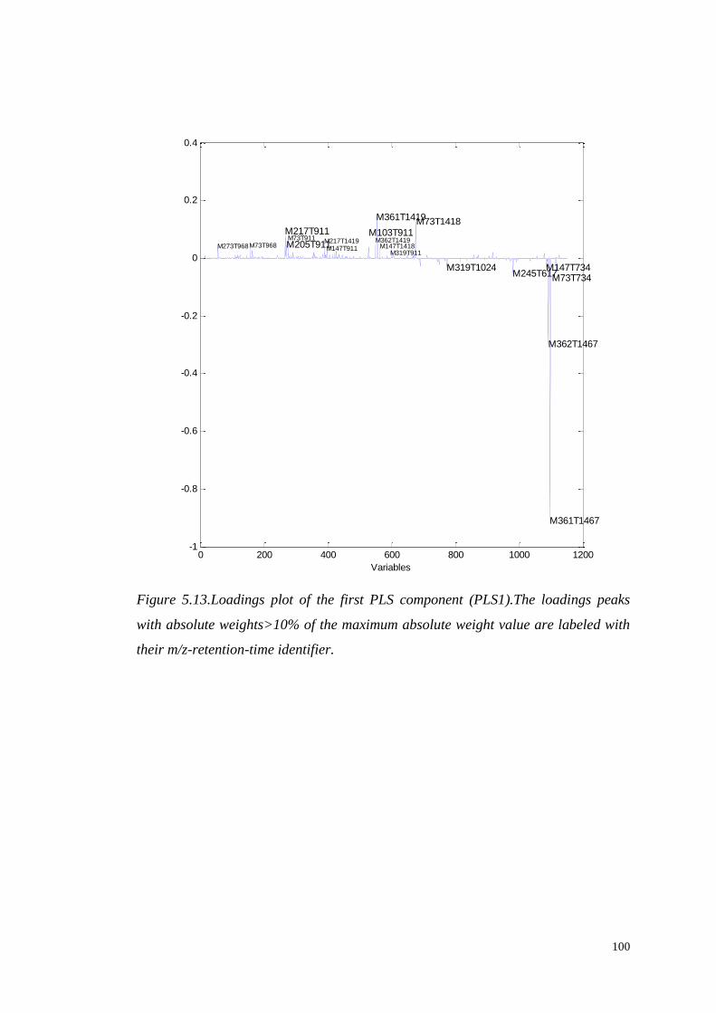
100
Figure 5.13.Loadings plot of the first PLS component (PLS1).The loadings peaks
with absolute weights>10% of the maximum absolute weight value are labeled with
their m/z-retention-time identifier.
0 200 400 600 800 1000 1200-1
-0.8
-0.6
-0.4
-0.2
0
0.2
0.4
Variables
M273T968M73T968
M217T911M217T1419M147T911
M361T1419M73T1418
M319T1024M245T617
M147T734
M362T1467
M361T1467
M73T734
M205T911
M103T911
M319T911M147T1418
M362T1419M73T911
101
Figure 5.14.Loadings plot of the second PLS component (PLS2).The loadings peaks
with absolute weights>10% of the maximum absolute weight value are labeled with
their m/z-retention-time identifier.
0 200 400 600 800 1000 1200-0.4
-0.3
-0.2
-0.1
0
0.1
0.2
0.3
0.4
0.5
M117T911M133T911
M217T911
M205T911
M73T911
M204T911
M206T911
M218T911
M219T911
M217T1419
M147T911
M103T911
M362T1419
M361T1419
M147T1418
M189T911
M319T911
M307T911
M73T1418
M73T1024
M129T911
M217T934M205T1024
M319T1024
M305T1137M204T1573
M75T617M143T617
M246T617
M245T617
M147T617
M73T617
M362T1467
M361T1467
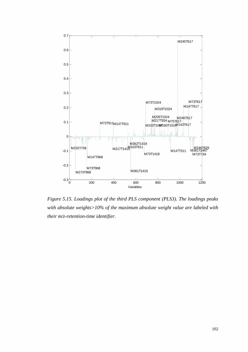
102
Figure 5.15. Loadings plot of the third PLS component (PLS3). The loadings peaks
with absolute weights>10% of the maximum absolute weight value are labeled with
their m/z-retention-time identifier.
0 200 400 600 800 1000 1200-0.3
-0.2
-0.1
0
0.1
0.2
0.3
0.4
0.5
0.6
0.7
M232T758
M273T968
M73T968
M147T968
M73T911
M217T1419
M147T911
M103T911M362T1419
M361T1419
M73T1418
M103T1007
M73T1024
M217T934M205T1024
M319T1024
M160T1024
M75T617
M147T311
M143T617
M246T617
M245T617
M147T617
M73T617
M361T1467M73T734
M246T829
Variables
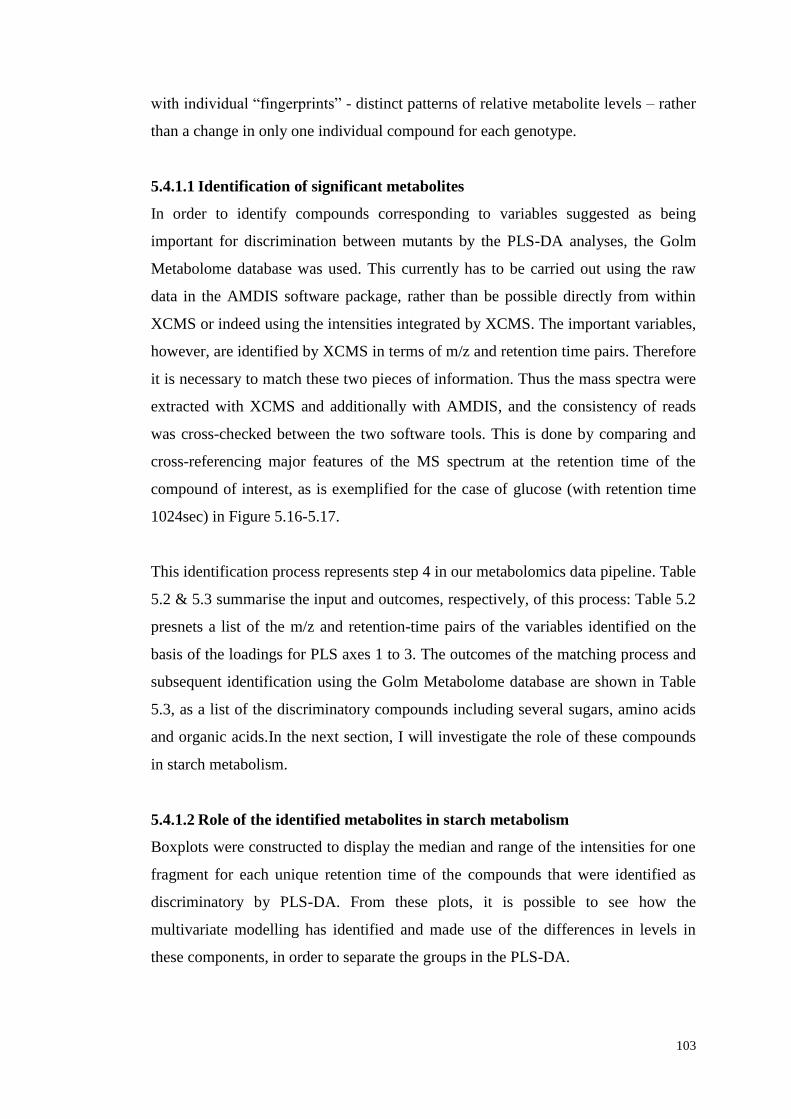
103
with individual “fingerprints” - distinct patterns of relative metabolite levels – rather
than a change in only one individual compound for each genotype.
5.4.1.1 Identification of significant metabolites
In order to identify compounds corresponding to variables suggested as being
important for discrimination between mutants by the PLS-DA analyses, the Golm
Metabolome database was used. This currently has to be carried out using the raw
data in the AMDIS software package, rather than be possible directly from within
XCMS or indeed using the intensities integrated by XCMS. The important variables,
however, are identified by XCMS in terms of m/z and retention time pairs. Therefore
it is necessary to match these two pieces of information. Thus the mass spectra were
extracted with XCMS and additionally with AMDIS, and the consistency of reads
was cross-checked between the two software tools. This is done by comparing and
cross-referencing major features of the MS spectrum at the retention time of the
compound of interest, as is exemplified for the case of glucose (with retention time
1024sec) in Figure 5.16-5.17.
This identification process represents step 4 in our metabolomics data pipeline. Table
5.2 & 5.3 summarise the input and outcomes, respectively, of this process: Table 5.2
presnets a list of the m/z and retention-time pairs of the variables identified on the
basis of the loadings for PLS axes 1 to 3. The outcomes of the matching process and
subsequent identification using the Golm Metabolome database are shown in Table
5.3, as a list of the discriminatory compounds including several sugars, amino acids
and organic acids.In the next section, I will investigate the role of these compounds
in starch metabolism.
5.4.1.2 Role of the identified metabolites in starch metabolism
Boxplots were constructed to display the median and range of the intensities for one
fragment for each unique retention time of the compounds that were identified as
discriminatory by PLS-DA. From these plots, it is possible to see how the
multivariate modelling has identified and made use of the differences in levels in
these components, in order to separate the groups in the PLS-DA.
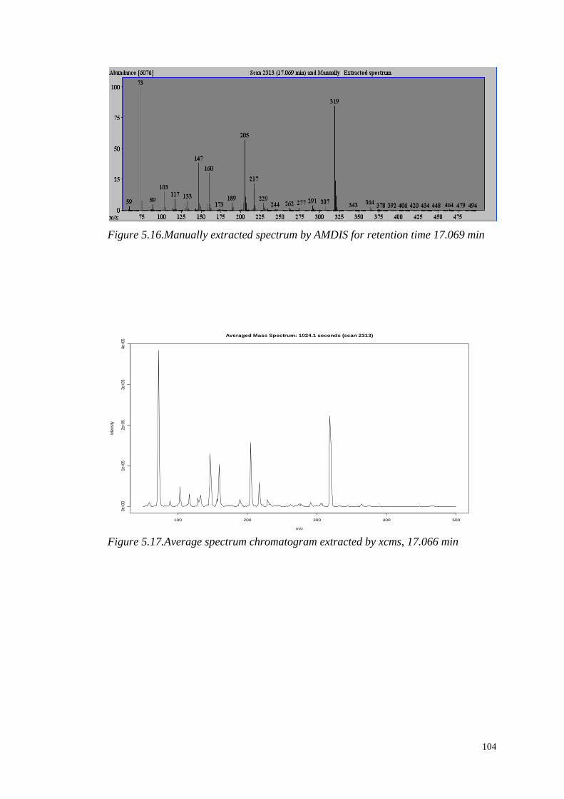
104
Figure 5.16.Manually extracted spectrum by AMDIS for retention time 17.069 min
Figure 5.17.Average spectrum chromatogram extracted by xcms, 17.066 min
100 200 300 400 500
0e+0
01e
+05
2e+0
53e
+05
4e+0
5
Averaged Mass Spectrum: 1024.1 seconds (scan 2313)
m/z
Inte
nsity
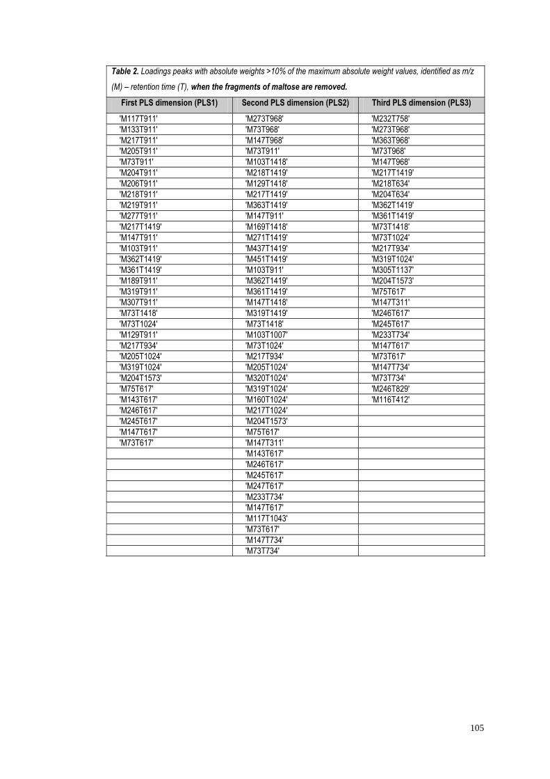
105
Table 2. Loadings peaks with absolute weights >10% of the maximum absolute weight values, identified as m/z
(M) – retention time (T), when the fragments of maltose are removed.
First PLS dimension (PLS1) Second PLS dimension (PLS2) Third PLS dimension (PLS3)
'M117T911' 'M273T968' 'M232T758'
'M133T911' 'M73T968' 'M273T968'
'M217T911' 'M147T968' 'M363T968'
'M205T911' 'M73T911' 'M73T968'
'M73T911' 'M103T1418' 'M147T968'
'M204T911' 'M218T1419' 'M217T1419'
'M206T911' 'M129T1418' 'M218T634'
'M218T911' 'M217T1419' 'M204T634'
'M219T911' 'M363T1419' 'M362T1419'
'M277T911' 'M147T911' 'M361T1419'
'M217T1419' 'M169T1418' 'M73T1418'
'M147T911' 'M271T1419' 'M73T1024'
'M103T911' 'M437T1419' 'M217T934'
'M362T1419' 'M451T1419' 'M319T1024'
'M361T1419' 'M103T911' 'M305T1137'
'M189T911' 'M362T1419' 'M204T1573'
'M319T911' 'M361T1419' 'M75T617'
'M307T911' 'M147T1418' 'M147T311'
'M73T1418' 'M319T1419' 'M246T617'
'M73T1024' 'M73T1418' 'M245T617'
'M129T911' 'M103T1007' 'M233T734'
'M217T934' 'M73T1024' 'M147T617'
'M205T1024' 'M217T934' 'M73T617'
'M319T1024' 'M205T1024' 'M147T734'
'M204T1573' 'M320T1024' 'M73T734'
'M75T617' 'M319T1024' 'M246T829'
'M143T617' 'M160T1024' 'M116T412'
'M246T617' 'M217T1024'
'M245T617' 'M204T1573'
'M147T617' 'M75T617'
'M73T617' 'M147T311'
'M143T617'
'M246T617'
'M245T617'
'M247T617'
'M233T734'
'M147T617'
'M117T1043'
'M73T617'
'M147T734'
'M73T734'
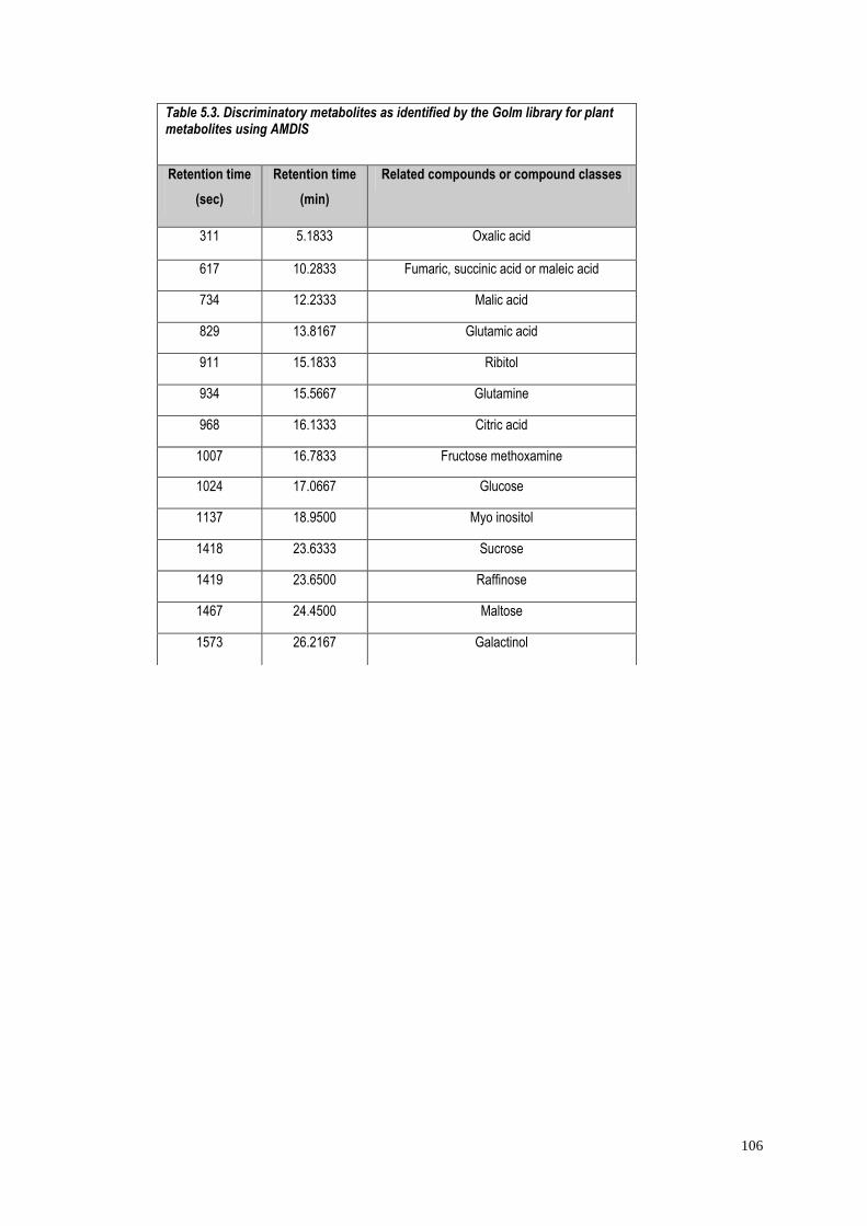
106
Table 5.3. Discriminatory metabolites as identified by the Golm library for plant metabolites using AMDIS
Retention time
(sec)
Retention time
(min)
Related compounds or compound classes
311 5.1833 Oxalic acid
617 10.2833 Fumaric, succinic acid or maleic acid
734 12.2333 Malic acid
829 13.8167 Glutamic acid
911 15.1833 Ribitol
934 15.5667 Glutamine
968 16.1333 Citric acid
1007 16.7833 Fructose methoxamine
1024 17.0667 Glucose
1137 18.9500 Myo inositol
1418 23.6333 Sucrose
1419 23.6500 Raffinose
1467 24.4500 Maltose
1573 26.2167 Galactinol
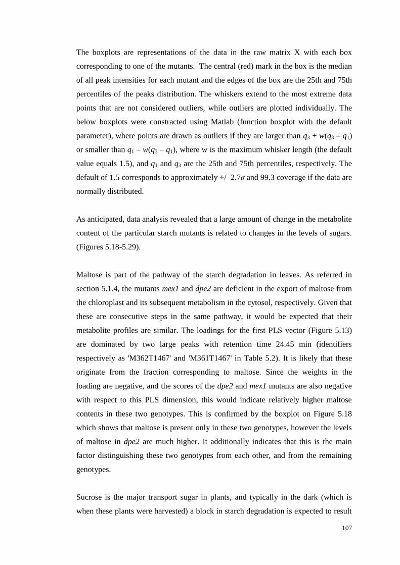
107
The boxplots are representations of the data in the raw matrix X with each box
corresponding to one of the mutants. The central (red) mark in the box is the median
of all peak intensities for each mutant and the edges of the box are the 25th and 75th
percentiles of the peaks distribution. The whiskers extend to the most extreme data
points that are not considered outliers, while outliers are plotted individually. The
below boxplots were constracted using Matlab (function boxplot with the default
parameter), where points are drawn as outliers if they are larger than q3 + w(q3 – q1)
or smaller than q1 – w(q3 – q1), where w is the maximum whisker length (the default
value equals 1.5), and q1 and q3 are the 25th and 75th percentiles, respectively. The
default of 1.5 corresponds to approximately +/–2.7σ and 99.3 coverage if the data are
normally distributed.
As anticipated, data analysis revealed that a large amount of change in the metabolite
content of the particular starch mutants is related to changes in the levels of sugars.
(Figures 5.18-5.29).
Maltose is part of the pathway of the starch degradation in leaves. As referred in
section 5.1.4, the mutants mex1 and dpe2 are deficient in the export of maltose from
the chloroplast and its subsequent metabolism in the cytosol, respectively. Given that
these are consecutive steps in the same pathway, it would be expected that their
metabolite profiles are similar. The loadings for the first PLS vector (Figure 5.13)
are dominated by two large peaks with retention time 24.45 min (identifiers
respectively as 'M362T1467' and 'M361T1467' in Table 5.2). It is likely that these
originate from the fraction corresponding to maltose. Since the weights in the
loading are negative, and the scores of the dpe2 and mex1 mutants are also negative
with respect to this PLS dimension, this would indicate relatively higher maltose
contents in these two genotypes. This is confirmed by the boxplot on Figure 5.18
which shows that maltose is present only in these two genotypes, however the levels
of maltose in dpe2 are much higher. It additionally indicates that this is the main
factor distinguishing these two genotypes from each other, and from the remaining
genotypes.
Sucrose is the major transport sugar in plants, and typically in the dark (which is
when these plants were harvested) a block in starch degradation is expected to result
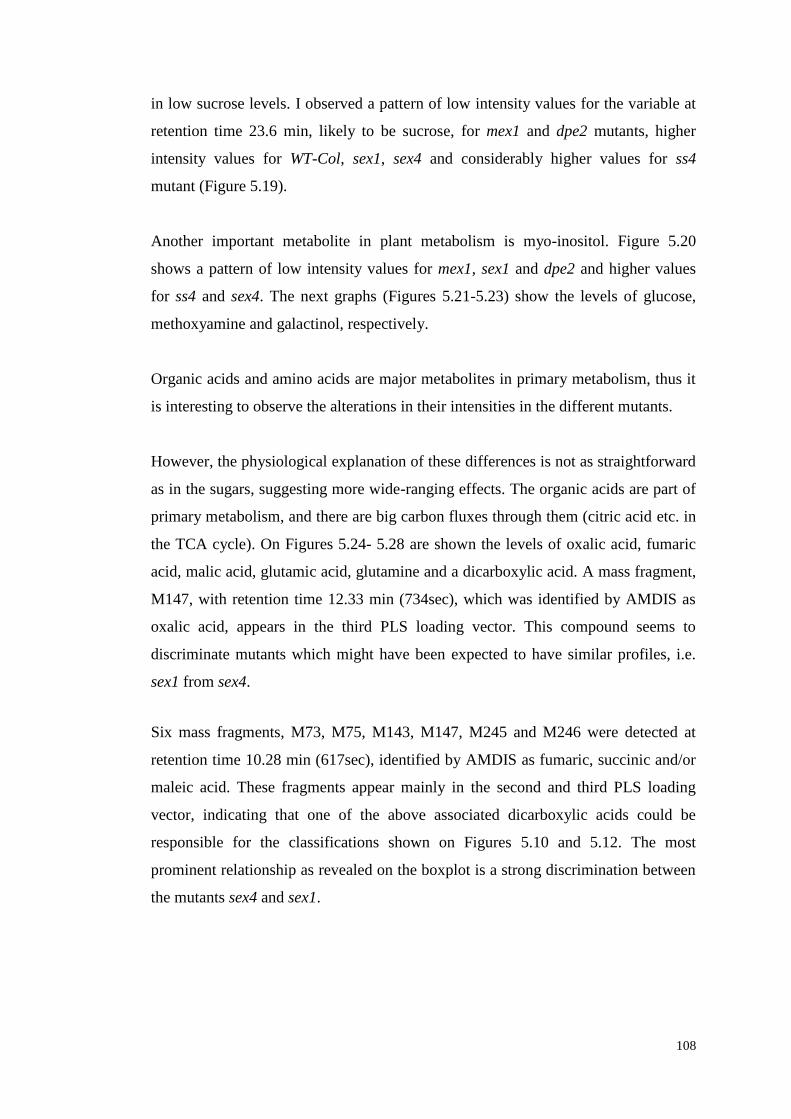
108
in low sucrose levels. I observed a pattern of low intensity values for the variable at
retention time 23.6 min, likely to be sucrose, for mex1 and dpe2 mutants, higher
intensity values for WT-Col, sex1, sex4 and considerably higher values for ss4
mutant (Figure 5.19).
Another important metabolite in plant metabolism is myo-inositol. Figure 5.20
shows a pattern of low intensity values for mex1, sex1 and dpe2 and higher values
for ss4 and sex4. The next graphs (Figures 5.21-5.23) show the levels of glucose,
methoxyamine and galactinol, respectively.
Organic acids and amino acids are major metabolites in primary metabolism, thus it
is interesting to observe the alterations in their intensities in the different mutants.
However, the physiological explanation of these differences is not as straightforward
as in the sugars, suggesting more wide-ranging effects. The organic acids are part of
primary metabolism, and there are big carbon fluxes through them (citric acid etc. in
the TCA cycle). On Figures 5.24- 5.28 are shown the levels of oxalic acid, fumaric
acid, malic acid, glutamic acid, glutamine and a dicarboxylic acid. A mass fragment,
M147, with retention time 12.33 min (734sec), which was identified by AMDIS as
oxalic acid, appears in the third PLS loading vector. This compound seems to
discriminate mutants which might have been expected to have similar profiles, i.e.
sex1 from sex4.
Six mass fragments, M73, M75, M143, M147, M245 and M246 were detected at
retention time 10.28 min (617sec), identified by AMDIS as fumaric, succinic and/or
maleic acid. These fragments appear mainly in the second and third PLS loading
vector, indicating that one of the above associated dicarboxylic acids could be
responsible for the classifications shown on Figures 5.10 and 5.12. The most
prominent relationship as revealed on the boxplot is a strong discrimination between
the mutants sex4 and sex1.
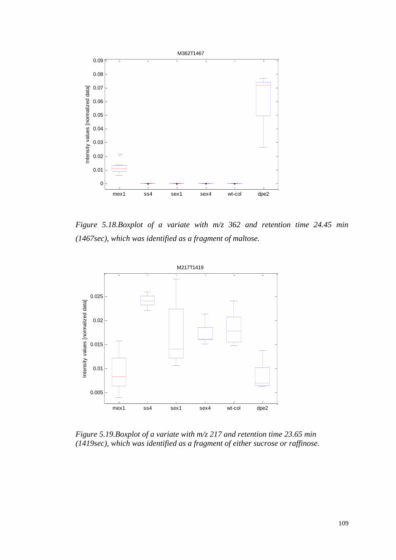
109
Figure 5.18.Boxplot of a variate with m/z 362 and retention time 24.45 min
(1467sec), which was identified as a fragment of maltose.
Figure 5.19.Boxplot of a variate with m/z 217 and retention time 23.65 min
(1419sec), which was identified as a fragment of either sucrose or raffinose.
mex1 ss4 sex1 sex4 wt-col dpe2
0
0.01
0.02
0.03
0.04
0.05
0.06
0.07
0.08
0.09
M362T1467
Inte
nsity v
alu
es [
norm
aliz
ed d
ata
]
mex1 ss4 sex1 sex4 wt-col dpe2
0.005
0.01
0.015
0.02
0.025
M217T1419
Inte
nsity v
alu
es [
norm
aliz
ed d
ata
]
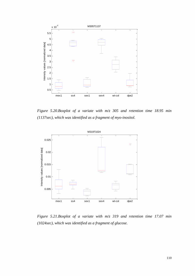
110
Figure 5.20.Boxplot of a variate with m/z 305 and retention time 18.95 min
(1137sec), which was identified as a fragment of myo-inositol.
Figure 5.21.Boxplot of a variate with m/z 319 and retention time 17.07 min
(1024sec), which was identified as a fragment of glucose.
mex1 ss4 sex1 sex4 wt-col dpe2
0.5
1
1.5
2
2.5
3
3.5
4
4.5
5
5.5
x 10-3 M305T1137
Inte
nsity v
alu
es [
norm
aliz
ed d
ata
]
mex1 ss4 sex1 sex4 wt-col dpe2
0.005
0.01
0.015
0.02
0.025
M319T1024
Inte
nsity v
alu
es [
norm
aliz
ed d
ata
]
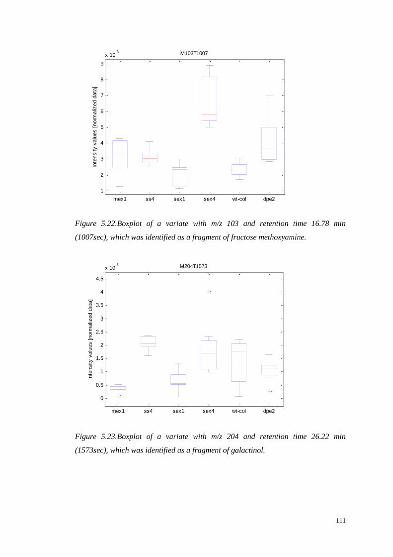
111
Figure 5.22.Boxplot of a variate with m/z 103 and retention time 16.78 min
(1007sec), which was identified as a fragment of fructose methoxyamine.
Figure 5.23.Boxplot of a variate with m/z 204 and retention time 26.22 min
(1573sec), which was identified as a fragment of galactinol.
mex1 ss4 sex1 sex4 wt-col dpe2
1
2
3
4
5
6
7
8
9
x 10-3 M103T1007
Inte
nsity v
alu
es [
norm
aliz
ed d
ata
]
mex1 ss4 sex1 sex4 wt-col dpe2
0
0.5
1
1.5
2
2.5
3
3.5
4
4.5
x 10-3 M204T1573
Inte
nsity v
alu
es [
norm
aliz
ed d
ata
]
112
Two unique mass fragments, M73 and M147, were detected at retention time 12.33
min (734sec), both of them identified as malic acid. These fragments appear in the
first and third PLS loading vectors, indicating that malic acid could contribute to the
discrimination of dpe2 and mex1 from the rest of the genotypes (Figure 5.10), or to
any of the relationships on the third PLS component (Figure 5.12), among which the
discrimination of sex1 and sex4 is most noticable on the boxplot below (Figure 5.26).
A mass fragment, M246, with retention time 13.82 min (829sec) identified by
AMDIS as L-glutamic acid, appears in the third PLS loading vector. However, the
boxplot (Figure 5.27) shows that there is large variance within each genotype, and
incomplete discrimination.
Finally, glutamate and glutamine are involved in carbon/nitrogen balance in plants. It
is found that glutamine is a clear discriminator between various genotypes (Figure
5.28). Glutamate did not reveal any strong relationship among the different
genotypes.
5.4.1.3 Summary of the mutant relationships
Maltose appears in significant concentrations only in the dpe2 and mex1 mutants,
with the highest levels in dpe2. Maltose has a very strong effect on the clustering
obtained by the supervised modelling. The effects of differences in the other
metabolite levels are somewhat more subtle. Raffinose and sucrose have relatively
high concentrations in the ss4 mutant, low concentrations in mex1 and dpe2, and
more intermediate concentrations for sex1, sex4, and wild type. The variable most
likely identified as fumaric acid has higher values for sex4 and very low for sex1,
indicating that it is a separator of the sex mutants. Myo-inositol exhibits high levels
for ss4 and sex4, lower levels for wild type, and very low for mex1, sex1 and dpe2.
Again this provides a differentiator between the sex1 and sex4 mutants.
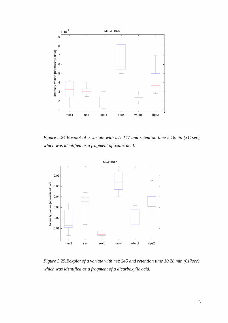
113
Figure 5.24.Boxplot of a variate with m/z 147 and retention time 5.18min (311sec),
which was identified as a fragment of oxalic acid.
Figure 5.25.Boxplot of a variate with m/z 245 and retention time 10.28 min (617sec),
which was identified as a fragment of a dicarboxylic acid.
mex1 ss4 sex1 sex4 wt-col dpe2
1
2
3
4
5
6
7
8
9
x 10-3 M103T1007
Inte
nsity v
alu
es [
norm
aliz
ed d
ata
]
mex1 ss4 sex1 sex4 wt-col dpe2
0
0.01
0.02
0.03
0.04
0.05
0.06
M245T617
Inte
nsity v
alu
es [
norm
aliz
ed d
ata
]
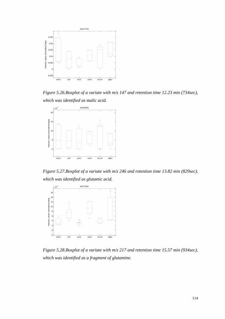
114
Figure 5.26.Boxplot of a variate with m/z 147 and retention time 12.23 min (734sec),
which was identified as malic acid.
Figure 5.27.Boxplot of a variate with m/z 246 and retention time 13.82 min (829sec),
which was identified as glutamic acid.
Figure 5.28.Boxplot of a variate with m/z 217 and retention time 15.57 min (934sec),
which was identified as a fragment of glutamine.
mex1 ss4 sex1 sex4 wt-col dpe2
-0.005
0
0.005
0.01
0.015
0.02
0.025
M147T734
Inte
nsity v
alu
es [
norm
aliz
ed d
ata
]
mex1 ss4 sex1 sex4 wt-col dpe2
0
5
10
15
20
x 10-3 M246T829
Inte
nsity v
alu
es [
norm
aliz
ed d
ata
]
mex1 ss4 sex1 sex4 wt-col dpe2-2
0
2
4
6
8
10
12
14
16
x 10-3 M217T934
Inte
nsity v
alu
es [
norm
aliz
ed d
ata
]
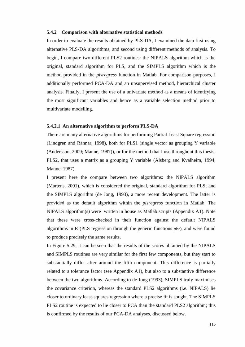
115
5.4.2 Comparison with alternative statistical methods
In order to evaluate the results obtained by PLS-DA, I examined the data first using
alternative PLS-DA algorithms, and second using different methods of analysis. To
begin, I compare two different PLS2 routines: the NIPALS algorithm which is the
original, standard algorithm for PLS, and the SIMPLS algorithm which is the
method provided in the plsregress function in Matlab. For comparison purposes, I
additionally performed PCA-DA and an unsupervised method, hierarchical cluster
analysis. Finally, I present the use of a univariate method as a means of identifying
the most significant variables and hence as a variable selection method prior to
multivariate modelling.
5.4.2.1 An alternative algorithm to perform PLS-DA
There are many alternative algorithms for performing Partial Least Square regression
(Lindgren and Rännar, 1998), both for PLS1 (single vector as grouping Y variable
(Andersson, 2009; Manne, 1987)), or for the method that I use throughout this thesis,
PLS2, that uses a matrix as a grouping Y variable (Alsberg and Kvalheim, 1994;
Manne, 1987).
I present here the compare between two algorithms: the NIPALS algorithm
(Martens, 2001), which is considered the original, standard algorithm for PLS; and
the SIMPLS algorithm (de Jong, 1993), a more recent development. The latter is
provided as the default algorithm within the plsregress function in Matlab. The
NIPALS algorithm(s) were written in house as Matlab scripts (Appendix A1). Note
that these were cross-checked in their function against the default NIPALS
algorithms in R (PLS regression through the generic functions plsr), and were found
to produce precisely the same results.
In Figure 5.29, it can be seen that the results of the scores obtained by the NIPALS
and SIMPLS routines are very similar for the first few components, but they start to
substantially differ after around the fifth component. This difference is partially
related to a tolerance factor (see Appendix A1), but also to a substantive difference
between the two algorithms. According to de Jong (1993), SIMPLS truly maximises
the covariance criterion, whereas the standard PLS2 algorithms (i.e. NIPALS) lie
closer to ordinary least-squares regression where a precise fit is sought. The SIMPLS
PLS2 routine is expected to lie closer to PCA than the standard PLS2 algorithm; this
is confirmed by the results of our PCA-DA analyses, discussed below.
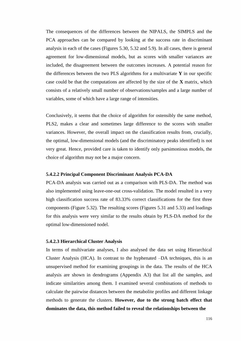
116
The consequences of the differences between the NIPALS, the SIMPLS and the
PCA approaches can be compared by looking at the success rate in discriminant
analysis in each of the cases (Figures 5.30, 5.32 and 5.9). In all cases, there is general
agreement for low-dimensional models, but as scores with smaller variances are
included, the disagreement between the outcomes increases. A potential reason for
the differences between the two PLS algorithms for a multivariate Y in our specific
case could be that the computations are affected by the size of the X matrix, which
consists of a relatively small number of observations/samples and a large number of
variables, some of which have a large range of intensities.
Conclusively, it seems that the choice of algorithm for ostensibly the same method,
PLS2, makes a clear and sometimes large difference to the scores with smaller
variances. However, the overall impact on the classification results from, crucially,
the optimal, low-dimensional models (and the discriminatory peaks identified) is not
very great. Hence, provided care is taken to identify only parsimonious models, the
choice of algorithm may not be a major concern.
5.4.2.2 Principal Component Discriminant Analysis PCA-DA
PCA-DA analysis was carried out as a comparison with PLS-DA. The method was
also implemented using leave-one-out cross-validation. The model resulted in a very
high classification success rate of 83.33% correct classifications for the first three
components (Figure 5.32). The resulting scores (Figures 5.31 and 5.33) and loadings
for this analysis were very similar to the results obtain by PLS-DA method for the
optimal low-dimensioned nodel.
5.4.2.3 Hierarchical Cluster Analysis
In terms of multivariate analyses, I also analysed the data set using Hierarchical
Cluster Analysis (HCA). In contrast to the hyphenated –DA techniques, this is an
unsupervised method for examining groupings in the data. The results of the HCA
analysis are shown in dendrograms (Appendix A3) that list all the samples, and
indicate similarities among them. I examined several combinations of methods to
calculate the pairwise distances between the metabolite profiles and different linkage
methods to generate the clusters. However, due to the strong batch effect that
dominates the data, this method failed to reveal the relationships between the
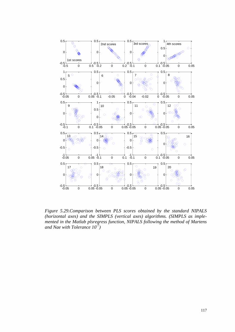
117
Figure 5.29.Comparison between PLS scores obtained by the standard NIPALS
(horizontal axes) and the SIMPLS (vertical axes) algorithms. (SIMPLS as imple-
mented in the Matlab plsregress function, NIPALS following the method of Martens
and Nae with Tolerance 10-7
)
-0.5 0 0.5-0.5
0
0.5
-0.2 0 0.2-0.5
0
0.5
-0.1 0 0.1-0.5
0
0.5
-0.05 0 0.05-0.5
0
0.5
1
-0.05 0 0.05-0.5
0
0.5
1
5
-0.1 -0.05 0-0.5
0
0.5
6
-0.04 -0.02 0-0.5
0
0.57
-0.05 0 0.05-0.5
0
0.58
-0.1 0 0.1-0.5
0
0.59
-0.05 0 0.05-0.5
0
0.5
110
-0.05 0 0.05-0.5
0
0.511
-0.05 0 0.05-0.5
0
0.512
-0.05 0 0.05-1
-0.5
0
0.513
-0.1 0 0.1-1
-0.5
0
0.514
-0.1 0 0.1-1
-0.5
0
0.515
-0.05 0 0.05-0.5
0
0.516
-0.05 0 0.05-0.5
0
0.517
-0.05 0 0.05-0.5
0
0.518
-0.05 0 0.05-0.5
0
0.5
19
-0.05 0 0.05-0.5
0
0.520
2nd scores 3rd scores 4th scores
1st scores
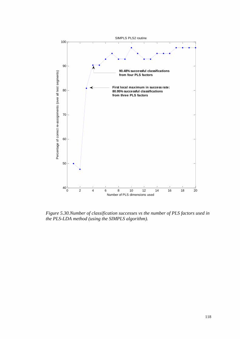
118
Figure 5.30.Number of classification successes vs the number of PLS factors used in
the PLS-LDA method (using the SIMPLS algorithm).
0 2 4 6 8 10 12 14 16 18 2040
50
60
70
80
90
100
Number of PLS dimensions used
Perc
enta
ge o
f corr
ect
re-a
ssig
nm
ents
(over
all
test
segm
ents
)
SIMPLS PLS2 routine
First local maximum in success rate:
80.95% successful classifications
from three PLS factors
90.48% successful classifications
from four PLS factors
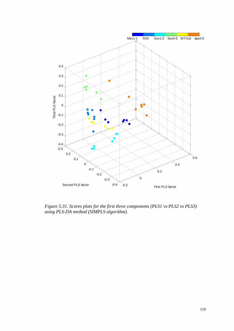
119
Figure 5.31. Scores plots for the first three components (PLS1 vs PLS2 vs PLS3)
using PLS-DA method (SIMPLS algorithm).
-0.2
0
0.2
0.4
0.6
-0.4
-0.3
-0.2
-0.1
0
0.1
0.2
0.3
-0.4
-0.3
-0.2
-0.1
0
0.1
0.2
0.3
0.4
First PLS factorSecond PLS factor
Third P
LS
facto
r
Mex1-1 SS4 Sex1-3 Sex4-3 WT-Col dpe2-5
120
mutants as a result of the genetic variation. The separation of dpe2 from the rest
of the mutants was the only clear observation of biological interest, which is
consistent with the results of the other statistical modelling analysis.
5.4.2.4 Univariate Multiway Analysis of Variance (Anova-n)
In addition to multivariate analysis, univariate analysis, in the form of multiway-
ANOVA, was carried out, as an alternative approach to identifying the most
important metabolites for discriminating between genotypes, through an individual
ranking method. As previously described, the starch dataset is dominated by a very
strong batch effect, thus besides the biological variability due to the different
genotypes, a univariate approach should also take into consideration the day of
analysis as an additional factor of variance. I used here an ANOVA model (anovan
function in Matlab) with two grouping variables: genotype and day of analysis. This
model computes p-values for each of the two grouping factors, and performs
multiple t-tests with Bonferroni adjustment to compensate for the multiple
comparisons. By specifying the suitable type of sum-of-squares (TypeI), the
calculations of the p-values in relation to the genotype (second term in anovan
function) are performed on a fit that already includes the effect of day (first term in
anovan function). In this way, finally a set of p-values that determine the most
significantly different variables (mz-RT time pairs) due to genotype after
compensating for the effect of day is obtained. The p-values of the 30 most
significantly different values are shown on Table 5.4. The unique retention times
identified here are 1467, 1137, 1418 and 1419 sec corresponding to fragments of
maltose, myoinositol, sucrose and raffinose respectively.
This result is consistent with the outcome of the PLS-DA analysis (Tables 5.2 and
5.3). However fewer compounds were identified, and no information about the
relationships between the mutants can be extracted; that is, there is no equivalent to
the PLS scores plot which depicts the relative positions of groups and observations
form one another in some chosen model space.
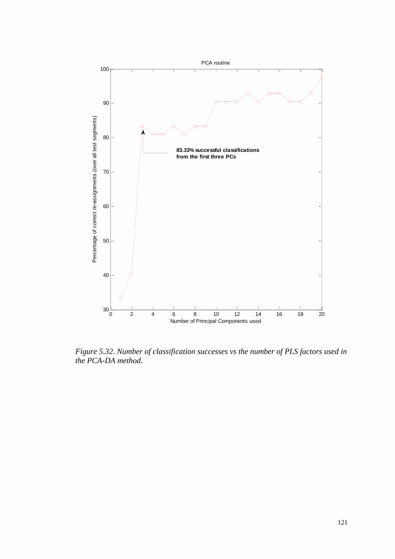
121
Figure 5.32. Number of classification successes vs the number of PLS factors used in
the PCA-DA method.
0 2 4 6 8 10 12 14 16 18 2030
40
50
60
70
80
90
100PCA routine
Number of Principal Components used
Perc
enta
ge o
f corr
ect
re-a
ssig
nm
ents
(over
all
test
segm
ents
)
83.33% successful classifications
from the first three PCs
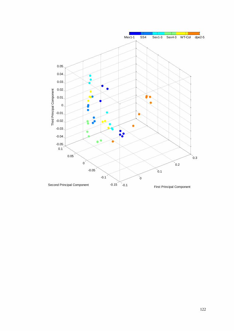
122
-0.1
0
0.1
0.2
0.3
-0.15
-0.1
-0.05
0
0.05
0.1
-0.05
-0.04
-0.03
-0.02
-0.01
0
0.01
0.02
0.03
0.04
0.05
First Principal ComponentSecond Principal Component
Third P
rincip
al C
om
ponent
Mex1-1 SS4 Sex1-3 Sex4-3 WT-Col dpe2-5
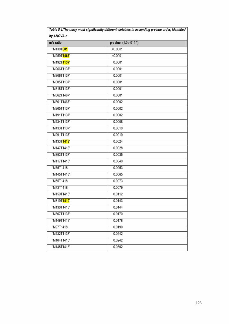
123
Table 5.4.Τhe thirty most significantly different variables in ascending p-value order, identified
by ANOVA-n
m/z ratio p-value (1.0e-011 *)
'M130T681' >0.0001
'M259T1467' >0.0001
'M192T1137' 0.0001
'M266T1137' 0.0001
'M306T1137' 0.0001
'M305T1137' 0.0001
'M318T1137' 0.0001
'M362T1467' 0.0001
'M361T1467' 0.0002
'M265T1137' 0.0002
'M191T1137' 0.0002
'M434T1137' 0.0008
'M433T1137' 0.0010
'M291T1137' 0.0019
'M133T1418' 0.0024
'M147T1418' 0.0028
'M393T1137' 0.0035
'M117T1418' 0.0040
'M75T1418' 0.0053
'M145T1418' 0.0065
'M55T1418' 0.0073
'M73T1418' 0.0079
'M159T1418' 0.0112
'M319T1419' 0.0143
'M130T1418' 0.0144
'M367T1137' 0.0170
'M149T1418' 0.0178
'M97T1418' 0.0190
'M432T1137' 0.0242
'M104T1418' 0.0242
'M148T1418' 0.0302
124
Anovan thus has somewhat limited capabilities compared to multivariate methods.
However, the method can be useful for comparative purposes, or could also be used
as a variable selection method prior to the multivariate methods. For instance, in the
whole data set of 1153 variables, only 451 variables passed the Bonferroni critical
value p<0.05/1153, forming a subset matrix of rank [42x451] that was subsequently
used as input for PLS-DA analysis.
5.5. Summary
This work has contributed to establishing relationships between the profiles of
different Arabidopsis starch mutant genotypes. I have successfully pre-processed
GC-MS data using an optimization method to select appropriate parameters for the
data type, and shown that the different supervised classification modelling methods
(multivariate and/or univariate) yielded similar results, and further, that
characterisation using XCMS and/or AMDIS is both practical and fruitful. I have
further seen that two PLS2 algorithms, NIPALS and SIMPLS, substantially differ
after the fourth component, despite being thought of as nominally the same
technique. It was clear that the data analysis is strongly affected by the batch effect
in this dataset, and that this effect needs to be taken into account by whatever
analysis method is adopted; hence, the unsupervised approach, HCA, did not
perform well, and was only able to make very limited statements about the data of
biological interest.

125
CHAPTER 6:
CONCLUSION
126
6 CONCLUSION
This thesis has examined the holistic process involved in metabolomics studies of
plant tissues, from data acquisition, through pre-processing and statistical analysis, to
interpretation of the results in biological terms. The motivation for the work was
specifically to address the implementation of the metabolomics “pipeline” at the
John Innes Centre; that is, to handle LC- and GC-MS data acquired in the main from
plant tissues. In the past, studies have largely focused on targeted analysis; manual
analysis of spectra using proprietary software Chemstation, Agilent Technology;
limited use of SIEVE; and statistical analyses mainly involving univariate, two-
groups comparisons. However, there is increasingly the requirement to perform
untargeted, metabolomics-scale analyses, with a greater range of options for data
analysis and interpretation.
I suggested a practical and functional software pipeline for MS metabolomics data
that comprises four main steps:
o the pre-processing of raw MS data using XCMS software
o the pre-treatment of the data via various scaling procedures (normalization,
centring, variance scaling)
o statistical analysis using one of the statistics-oriented, open source
programming languages (R, Matlab)
o the annotation of metabolite signals using on-line libraries
The key feature of this pipeline is that it is flexible and open-source. This implies
that it avoids the disadvantages associated with instrument-specific software which
are often expensive and non-transferable between machines. Moreover, all the
methods and algorithms involved in the pipeline are transparent, which means they
can be checked for correctness, or easily altered to adapt to different
experiments/instruments.
I believe that this pipeline can be used extensively for the analysis of metabolomic
experiments in the future, and will lead to fruitful results by helping to decode
complex biological phenomena. Moreover, considering that the pipeline is flexible
and adaptable to different technologies, with the right implementations it can be used
127
for merging data of different natures and structures. It is anticipated that a robust
analysis of metabolomic data will be very important for the integration of
metabolomics with other ‘omic technologies, such as transcriptomics and
proteomics.
All software elements in the pipeline are flexible and open source. Two
programming platforms were employed for various different steps. The pre-
processing step was conducted using XCMS software in the freely available ‘R’
environment. Pre-treatment and statistical analyses were conducted using ‘R’, and
the commercial language, Matlab (The Mathworks, Inc). Comparisons and contrasts
were made between alternative statistical methods, as well as across different
implementations of the same method. Thus, the open source nature of both languages
was fully exploited.
Some specific features of various components of the pipeline were investigated in
detail, at the level of coding of the algorithms, and revisions and improvements were
developed. For example, one element of the initial work was the revision of the
default algorithms for PLS in R, which as of July 2009 did not provide cross-
validated scores. It was possible to write a revised and updated routine to provide
this functionality; eventually this may be uploaded to the ‘R’ project as a user
contribution.
The statistical modelling step involves a choice of multivariate/univariate and
supervised/unsupervised methods, with an emphasis on appropriate model
validation. Particular attention was given to a commonly encountered chemometric
method, Partial Least Squares Discriminant Analysis (PLS-DA). Consideration was
given to different variants of the PLS algorithm, and it was shown these can impact
quite substantially on the outcome of analyses. However, although methodological
and even algorithm differences produced numerically quite different results, I found
that the final outcomes of the alternative supervised modelling techniques in terms of
biological interpretation were very similar.
Two particular experimental data sets have been examined in detail, both acquired
from specimens of Arabidopsis wild-type and mutant plants. The first dataset
128
(HiMet, Chapter 4) of LC-MS data was used to demonstrate some considerations for
specific steps of the pipeline, whilst the second dataset (Starch mutant analysis,
Chapter 5) comprising GC-MS data was used for a thorough presentation of the
pipeline.
In Chapter 4, I demonstrated that PLS-DA can be effectively used for the
classification of a set of Arabidopsis mutants, and can make predictions on the
identity of mutants with unknown functionalities (SMlines). I used this Chapter to
introduce important pre-treatment steps and emphasize the importance of validation
steps in the modelling process, which can avoid such phenomena as overfitting.
In Chapter 5, I presented XCMS as the software of choice for data pre-processing.
XCMS by default is optimized for LC-MS analysis. A challenge was to thoroughly
understand the various pre-processing functions as implemented within XCMS,
rather than using the software as a black box, and to identify key parameters that
should be optimized for the use of the software for GC-MS analysis. In this work I
established non-default parameters for GC-MS analysis, concerning the
chromatographic peak width (fwhm) and an across-samples grouping parameter (bw).
In contrast with literature reports (Danielson et al., 2002) which assert that these
parameters do not substantially affect the peak extraction process, I found that
incorrect parameter settings could reduce the number of compounds identified by up
to half.
An important observation regarding the data acquisition was that in all the data
examined, experimental effects (batching, machine drift) had a considerable impact
on the data. The observed batch effect (day-of-analysis effect) observed in starch
mutants analysis (Chapter 5) suggested that a careful instrument operation is
essential for the quality of the data. Nevertheless, multivariate analysis was in all
cases able to generate models which were able to discriminate between the different
groups (genotypes) under study, which indicates that the methods suggested are very
powerful for the analysis of ‘systematically noisy’ data.
The output from the analysis of the starch mutants in Chapter 5 indicated key
metabolites responsible for the difference between groups of samples. Some of the
129
putatively identified compounds were consistent with anticipated differences
between sample types, confirming the effectiveness of the statistical approach.
Additionally, some less anticipated compounds were identified as key
discriminators. These results can be used as a strong indicator of the relationships
underlying the particular pathways. However it should be emphasized that the data
are taken from a single time point, and that the results from a single experiment can
be used only as circumstantial evidence of the underlying relationships. Future
experiments could involve a wider range of mutants, as well as measurements from
different time points, the use of different extraction methods, and the combinations
of different technologies. For example, a wider range of mutations would improve
our understanding of the effect of genes on the metabolic phenotype by providing a
better coverage of the metabolic effects of mutations. In addition, considering that
variations in starch content can be observed throughout the diurnal cycle,
investigating the metabolome at different time points during the diurnal cycle (e.g. at
the end of the light period) and at different stages of plant growth would facilitate a
better understanding of starch metabolism.
In conclusion, the use of metabolomics to decipher complex metabolic processes
requires detailed understanding of the system under study, of the measurement
technologies and their specific impact on the data produced, and of data handling and
statistical techniques suitable for very large datasets. At this moment in time, this is
far from an automated process that can reveal hidden patterns of biological interest
just by feeding raw metabolomic data; instead, a thorough understanding of each of
the steps involved in the pipeline by the researchers working with the data is crucial.

130
CHAPTER 7:
LITERATURE CITED
131
7 LITERATURE CITED
Alsberg B.K., Kvalheim O.M. (1994) Speed improvement of multivariate algorithms
by the method of postponed basis matrix multiplication: Part I. Principal
component analysis. Chemometrics and Intelligent Laboratory Systems
24:31-42.
Andersson M. (2009) A comparison of nine PLS1 algorithms. Journal of
Chemometrics 23:518-529.
Bais P., Moon S.M., He K., Leitao R., Dreher K., Walk T., Sucaet Y., Barkan L.,
Wohlgemuth G., Roth M.R. (2010) PlantMetabolomics. org: a web portal for
plant metabolomics experiments. Plant Physiology 152:1807-1816.
Beck E., Ziegler P. (1989). Biosynthesis and degradation of starch in higher plants.
Annual Review of Plant Biology 40:95-117.
Bijlsma S., Bobeldijk I., Verheij E.R., Ramaker R., Kochhar S., Macdonald I.A., van
Ommen B., Smilde A.K. (2006) Large-scale human metabolomics studies: a
strategy for data (pre-) processing and validation. Analytical Chemistry
78:567-574.
Bino R.J., Hall R.D., Fiehn O., Kopka J., Saito K., Draper J., Nikolau B.J., Mendes
P., Roessner-Tunali U., Beale M.H. (2004) Potential of metabolomics as a
functional genomics tool. Trends in Plant Science 9:418-425.
Blackburn G., Zheng L.,Watson D. (2010) Data processing methods in
metabolomics. (Poster) Available from:
http://www.metabolomics.strath.ac.uk/files/ media/SUSLA_facilities_poster_
07042010.pdf
Broadhurst D.I., Kell D.B. (2006) Statistical strategies for avoiding false discoveries
in metabolomics and related experiments. Metabolomics, 2: 171-196.
Boccard J., Veuthey J.L., Rudaz S. (2010) Knowledge discovery in metabolomics:
an overview of MS data handling. Journal of Separation Science 33:290-304.
Boyes D.C., Zayed A.M., Ascenzi R., McCaskill A.J., Hoffman N.E., Davis K.R.,
Görlach J. (2001) Growth stage–based phenotypic analysis of Arabidopsis: A
model for high throughput functional genomics in plants. The Plant Cell
13:1499-1510.
Buléon A., Colonna P., Planchot V., Ball S. (1998) Starch granules: structure and
biosynthesis. International Journal of Biological Macromolecules 23:85-112.
132
Canelas A.B., ten Pierick A., Ras C., Seifar R.M., van Dam J.C., van Gulik W.M.,
Heijnen J.J. (2009) Quantitative evaluation of intracellular metabolite
extraction techniques for yeast metabolomics. Analytical Chemistry 81:7379-
7389.
Chia T., Thorneycroft D., Chapple A., Messerli G., Chen J., Zeeman S.C., Smith
S.M., Smith A.M. (2004) A cytosolic glucosyltransferase is required for
conversion of starch to sucrose in Arabidopsis leaves at night. The Plant
Journal 37:853-863.
Cole R.B. (1997) Electrospray ionization mass spectrometry: fundamentals,
instrumentation, and applications. Wiley, ISBN: 0-471-14564-5, New York,
USA.
Corrado E.M. (2005) The importance of open access, open source, and open
standards for libraries. Issues in Science and Technology Librarianship, 42
Spring Issue 2005.
Craig A., Cloarec O., Holmes E., Nicholson J.K., Lindon J.C. (2006) Scaling and
normalization effects in NMR spectroscopic metabonomic data sets.
Analytical Chemistry 78:2262-2267.
de Hoffmann E., Stroobant V. (2002) Mass spectrometry: principles and
applications. Second edition. Wiley. ISBN: 0-471-48566-7, Chichester, UK.
de Jong S. (1993) SIMPLS: an alternative approach to partial least squares
regression. Chemometrics and Intelligent Laboratory Systems 18:251-263.
Danielsson R., Bylund D., Markides K.E. (2002) Matched filtering with background
suppression for improved quality of base peak chromatograms and mass
spectra in liquid chromatography-mass spectrometry. Analytica Chimica Acta
454:167-184.
Defernez M., Kemsley E.K. (1997) The use and misuse of chemometrics for treating
classification problems. Trends in Analytical Chemistry 16, 216-221.
Dettmer K., Aronov P.A., Hammock B.D. (2007) Mass spectrometry-based
metabolomics. Mass Spectrometry Reviews 26:51-78.
Díaz Cruz M.S., López de Alda M.J., López R., Barceló D. (2003) Determination of
estrogens and progestogens by mass spectrometric techniques (GC/MS,
LC/MS and LC/MS/MS). Journal of Mass Spectrometry 38:917-923.
Dunn W.B., Ellis D. (2005) Metabolomics: current analytical platforms and
methodologies. TrAC Trends in Analytical Chemistry 24:285-294.
133
Elizabeth J., O'Maille G., Smith C.A., Brandon T.R., Uritboonthai W., Qin C.,
Trauger S.A., Siuzdak G. (2006) Solvent-dependent metabolite distribution,
clustering, and protein extraction for serum profiling with mass spectrometry.
Analytical Chemistry 78:743-752.
Eriksson L., Johansson E., Kettaneh-Wold N., Wold S. (2001) Multi-and
megavariate data analysis. Umetrics Academy, ISBN: 91-973730-1, Umeå,
Sweden.
Exarchou V., Godejohann M., van Beek T.A., Gerothanassis I.P., Vervoort J. (2003)
LC-UV-solid-phase extraction-NMR-MS combined with a cryogenic flow
probe and its application to the identification of compounds present in Greek
oregano. Analytical Chemistry 75:6288-6294.
Fernie A.R., Schauer N. (2009) Metabolomics-assisted breeding: a viable option for
crop improvement. Trends Genetics 25:39-48.
Fiehn O. (2002) Metabolomics–the link between genotypes and phenotypes. Plant
Molecular Biology 48:155-171.
Fiehn O., Kopka J., Dormann P., Altmann T., Trethewey R.N., Willmitzer L. (2000)
Metabolite profiling for plant functional genomics. Nature Biotechnology
18:1157-1161.
Fiehn O., Wohlgemuth G., Scholz M., Kind T., Lee D.Y., Lu Y., Moon S., Nikolau
B. (2008) Quality control for plant metabolomics: reporting MSI compliant
studies. The Plant Journal 53:691-704.
Geladi P. (1988) Notes on the history and nature of partial least squares (PLS)
modelling. Journal of Chemometrics 2:231-246.
Gentleman R.C., Carey V.J., Bates D.M., Bolstad B., Dettling M., Dudoit S., Ellis
B., Gautier L., Ge Y., Gentry J. (2004) Bioconductor: open software
development for computational biology and bioinformatics. Genome Biology
5:R80.
Goodacre R., Broadhurst D., Smilde A.K., Kristal B.S., Baker J.D., Beger R.,
Bessant C., Connor S., Capuani G., Craig A. (2007) Proposed minimum
reporting standards for data analysis in metabolomics. Metabolomics 3:231-
241.
Goodacre R., Vaidyanathan S., Dunn W.B., Harrigan G.G., Kell D.B. (2004)
Metabolomics by numbers: acquiring and understanding global metabolite
data. Trends in Biotechnology 22:245-252.
134
Hagel J.M., Facchini P.J. (2008) Plant metabolomics: analytical platforms and
integration with functional genomics. Phytochemistry Reviews 7:479-497.
Hall R.D. (2006) Plant metabolomics: from holistic hope, to hype, to hot topic. New
Phytologist 169:453-468.
Hollywood K., Brison D.R., Goodacre R. (2006) Metabolomics: current technologies
and future trends. Proteomics 6:4716-4723.
Hummel J., Selbig J., Walther D., Kopka J. (2007) The Golm Metabolome Database:
a database for GC-MS based metabolite profiling. Metabolomics 18:75-95.
Idborg H., Zamani L., Edlund P.O., Schuppe-Koistinen I., Jacobsson S.P. (2005)
Metabolic fingerprinting of rat urine by LC/MS: Part 2. Data pretreatment
methods for handling of complex data. Journal of Chromatography B
828:14-20.
Jander G., Norris S.R., Joshi V., Fraga M., Rugg A., Yu S., Li L., Last R.L. (2004)
Application of a high throughput HPLC MS/MS assay to Arabidopsis mutant
screening; evidence that threonine aldolase plays a role in seed nutritional
quality. The Plant Journal 39:465-475.
Jenkins H., Hardy N., Beckmann M., Draper J., Smith A. R., Taylor J., Fiehn O.,
Goodacre R., Bino R.J., Hall R., Kopka J., Lane G.A., Lange M.B., Liu J.R.,
Mendes P., Nikolau B.J., Oliver S.G., Paton N.W., Rhee S., Roessner-Tunali
U., Saito K., Smedsgaard J., Sumner L.W., Wang T., Walsh S., Wurtele E.S.,
Kell D.B (2004) A proposed framework for the description of plant
metabolomics. Nature Biotechnology 22:1601-1606.
Johnson H.E., Broadhurst D., Kell D.B., Theodorou M.K., Merry R.J., Griffith G.W.
(2004) High-throughput metabolic fingerprinting of legume silage
fermentations via Fourier transform infrared spectroscopy and chemometrics.
Applied and Environmental Microbiology 70:1583-1592.
Jonsson P., Johansson A.I., Gullberg J., Trygg J., Jiye A., Grung B., Marklund S.,
Sjöström M., Antti H., Moritz T. (2005) High-throughput data analysis for
detecting and identifying differences between samples in GC/MS-based
metabolomic analyses. Analytical Chemistry 77:5635-5642.
Kaplan F., Kopka J., Haskell D.W., Zhao W., Schiller K.C., Gatzke N., Sung D.Y.,
Guy C.L. (2004) Exploring the temperature-stress metabolome of
Arabidopsis. Plant Physiology 136:4159-4168.
135
Katajamaa M., Miettinen J., Oreši M. (2006) MZmine: toolbox for processing and
visualization of mass spectrometry based molecular profile data.
Bioinformatics 22:634-636.
Katajamaa M., Oresic M. (2007) Data processing for mass spectrometry-based
metabolomics. Journal of Chromatography A 1158:318-328.
Kemsley E. (1996) Discriminant analysis of high-dimensional data: a comparison of
principal components analysis and partial least squares data reduction
methods. Chemometrics and Intelligent Laboratory Systems 33:47-61.
Keun H.C., Ebbels T., Antti H., Bollard M.E., Beckonert O., Holmes E., Lindon
J.C., Nicholson J.K. (2003) Improved analysis of multivariate data by
variable stability scaling: application to NMR-based metabolic profiling.
Analytica Chimica Acta 490:265-276.
Keurentjes J.J.B. (2009) Genetical metabolomics: closing in on phenotypes. Current
Opinion in Plant Biology 12:223-230.
Kopka J. (2006) Current challenges and developments in GC-MS based metabolite
profiling technology. Journal of Biotechnology 124:312-322.
Krishnan P., Kruger N.J., Ratcliffe R.G. (2005) Metabolite fingerprinting and
profiling in plants using NMR. Journal of Experimental Botany 56:255-265.
Krishnan P., Kruger N.J., Ratcliffe R.G. (2005) Metabolite fingerprinting and
profiling in plants using NMR. Journal of Experimental Botany 56:255-265.
Last R.L., Jones A.D., Shachar-Hill Y. (2007) Towards the plant metabolome and
beyond. Nature Reviews Molecular Cell Biology 8:167-174.
Lin C.Y., Wu H.F., Tjeerdema R.S., Viant M.R. (2007) Evaluation of metabolite
extraction strategies from tissue samples using NMR metabolomics.
Metabolomics 3:55-67.
Lindgren F., Rännar S. (1998) Alternative partial least-squares (PLS) algorithms.
Perspectives in Drug Discovery and Design 12:105-113.
Lommen A. (2009) MetAlign: interface-driven, versatile metabolomics tool for
hyphenated full-scan mass spectrometry data preprocessing. Analytical
Chemistry 81:3079-3086.
Major H., Plumb R. (2006) A pragmatic and readily implemented quality control
strategy for HPLC-MS and GC-MS-based metabonomic analysis. Analyst
131:1075-1078.
136
Manne R. (1987) Analysis of two partial-least-squares algorithms for multivariate
calibration. Chemometrics and Intelligent Laboratory Systems 2:187-197.
Martens H. (2001) Reliable and relevant modelling of real world data: a personal
account of the development of PLS regression. Chemometrics and Intelligent
Laboratory Systems 58:85-95.
Messerli G., Partovi Nia V., Trevisan M., Kolbe A., Schauer N., Geigenberger P.,
Chen J., Davison A.C., Fernie A.R., Zeeman S.C. (2007) Rapid classification
of phenotypic mutants of Arabidopsis via metabolite fingerprinting. Plant
Physiology 143:1484.
Miyashita Y., Itozawa T., Katsumi H., Sasaki S.I. (1990) Comments on the NIPALS
algorithm. Journal of Chemometrics 4:97-100.
Moco S., Bino R.J., De Vos R.C.H., Vervoort J. (2007) Metabolomics technologies
and metabolite identification. TrAC Trends in Analytical Chemistry 26:855-
866.
Moco S., Schneider B., Vervoort J. (2009) Plant Micrometabolomics: the analysis of
endogenous metabolites present in a plant cell or tissue. Journal of Proteome
Research 8:1694-1703.
Moco S., Vervoort J., Bino R.J., De Vos R.C.H., Bino R. (2007) Metabolomics
technologies and metabolite identification. TrAC Trends in Analytical
Chemistry 26:855-866.
Mueller L.N., Brusniak M.Y., Mani D., Aebersold R. (2008) An assessment of
software solutions for the analysis of mass spectrometry based quantitative
proteomics data. Journal of Proteome Research 7:51-61.
Mueller L.A., Zhang P., Rhee S.Y. (2003) AraCyc: a biochemical pathway database
for Arabidopsis. Plant Physiology 132:453-460.
Niittylä T., Messerli G., Trevisan M., Chen J., Smith A.M., Zeeman S.C. (2004) A
previously unknown maltose transporter essential for starch degradation in
leaves. Science 303:87-89.
Nunes Nesi A., Sweetlove L.J., Fernie A.R. (2007) Operation and function of the
tricarboxylic acid cycle in the illuminated leaf. Physiologia Plantarum
129:45-56.
Oksman-Caldentey K.M., Saito K. (2005) Integrating genomics and metabolomics
for engineering plant metabolic pathways. Current Opinion in Biotechnology
16:174-179.
137
Okuda S., Yamada T., Hamajima M., Itoh M., Katayama T., Bork P., Goto S.,
Kanehisa M. (2008) KEGG atlas mapping for global analysis of metabolic
pathways. Nucleic Acids Research 36:W423-426.
Oliver S.G., Winson M.K., Kell D.B., Baganz F. (1998) Systematic functional
analysis of the yeast genome. Trends in Biotechnology 16:373-378.
Pearson K. (1901) Principal components analysis. The London, Edinburgh, and
Dublin Philosophical Magazine and Journal of Science 6:559.
Ratcliffe R.G., Shachar-Hill Y. (2005) Revealing metabolic phenotypes in plants:
inputs from NMR analysis. Biological Reviews 80:27-43.
Redestig H., Szymanski J., Hirai M.Y., Selbig J., Willmitzer L., Nikoloski Z., Saito
K. (2011) Data integration, metabolic networks and systems biology. Anual
Plant Review 43: Biology of Plant Metabolomics.
Rew R., Davis G. (1990) NetCDF: an interface for scientific data access. Computer
Graphics and Applications, IEEE 10:76-82.
Rochfort S. (2005) Metabolomics reviewed: a new “omics” platform technology for
systems biology and implications for natural products research. Journal of
Natural Products 68:1813-1820.
Roessner U., Luedemann A., Brust D., Fiehn O., Linke T., Willmitzer L., Fernie
A.R. (2001) Metabolic profiling allows comprehensive phenotyping of
genetically or environmentally modified plant systems. The Plant Cell
13:11-29.
Roessner U., Wagner C., Kopka J., Trethewey R.N., Willmitzer L. (2000)
Simultaneous analysis of metabolites in potato tuber by gas chromatography–
mass spectrometry. The Plant Journal 23:131-142.
Rosipal R., Krämer N. (2006) Overview and recent advances in partial least squares.
Subspace, Latent Structure and Feature Selection 3940:34-51.
Saito K., Matsuda F. (2010) Metabolomics for functional genomics, systems
biology, and biotechnology. Annual Review of Plant Biology 61:463-489.
Schauer N., Fernie A.R. (2006) Plant metabolomics: towards biological function and
mechanism. Trends in Plant Science 11:508-516.
Schauer N., Steinhauser D., Strelkov S., Schomburg D., Allison G., Moritz T.,
Lundgren K., Roessner-Tunali U., Forbes M.G., Willmitzer L. (2005) GC-
MS libraries for the rapid identification of metabolites in complex biological
samples. FEBS letters 579:1332-1337.
138
Scott I.M., Vermeer C.P., Liakata M., Corol D.I., Ward J.L., Lin W., Johnson H.E.,
Whitehead L., Kular B., Baker J.M. (2010) Enhancement of plant metabolite
fingerprinting by machine learning. Plant Physiology 153:1506-1520.
Shah V.P., Midha K.K., Findlay J.W.A., Hill H.M., Hulse J.D., McGilveray I.J.,
McKay G., Miller K.J., Patnaik R.N., Powell M.L. (2000) Bioanalytical
method validation—a revisit with a decade of progress. Pharmaceutical
Research 17:1551-1557.
Smith A.M., Denyer K., Martin C. (1997) The synthesis of the starch granule.
Annual Review of Plant Biology 48:67-87.
Smith A.M., Zeeman S.C., Smith S.M. (2005) Starch degradation. Annual Review of
Plant Biology 56:73-98.
Smith C.A., Elizabeth J., O'Maille G., Abagyan R., Siuzdak G. (2006) XCMS:
processing mass spectrometry data for metabolite profiling using nonlinear
peak alignment, matching, and identification. Analytical Chemistry 78:779-
787.
Stitt M., Fernie A.R. (2003) From measurements of metabolites to metabolomics: an
‘on the fly’ perspective illustrated by recent studies of carbon-nitrogen
interactions. Current Opinion in Biotechnology 14:136-144.
Styczynski M.P., Moxley J.F., Tong L.V., Walther J.L., Jensen K.L.,
Stephanopoulos G.N. (2007) Systematic identification of conserved
metabolites in GC/MS data for metabolomics and biomarker discovery.
Analytical Chemistry 79:966-973.
Sysi-Aho M., Katajamaa M., Yetukuri L., Oreši M. (2007) Normalization method
for metabolomics data using optimal selection of multiple internal standards.
BMC Bioinformatics 8:93.
Terabe S., Markuszewski M.J., Inoue N., Otsuka K., Nishioka T. (2001) Capillary
electrophoretic techniques toward the metabolome analysis. Pure and
Applied Chemistry 73:1563-1572.
Trygg J., Gullberg J., Johansson A., Jonsson P., Moritz T. (2006) Chemometrics in
metabolomics—an introduction. Plant Metabolomics 57:117-128.
Tweeddale H., Notley-McRobb L., Ferenci T. (1998) Effect of slow growth on
metabolism of Escherichia coli, as revealed by global metabolite pool ("
metabolome") analysis. Journal of Bacteriology 180:5109-5116.
139
Van Den Berg R.A., Hoefsloot H.C.J., Westerhuis J.A., Smilde A.K., Van Der Werf
M.J. (2006) Centering, scaling, and transformations: improving the biological
information content of metabolomics data. BMC Genomics 7:142.
van der Greef J., Smilde A.K. (2005) Symbiosis of chemometrics and metabolomics:
past, present, and future. Journal of Chemometrics 19:376-386.
van Zijtveld J., van den Berg S., Swart P. (2003) Development and validation of a
direct plasma injection LC-MS method for YM087 and YM440 and
metabolites in human plasma. Chromatographia 57:23-27.
Weckwerth W. (2003) Metabolomics in systems biology. Annual Review of Plant
Biology 54:669-689.
Weckwerth W. (2007) Metabolomics: methods and protocols. Humana Press,
ISBN:1064-3745, New Jersey.
Weckwerth W., Morgenthal K. (2005) Metabolomics: from pattern recognition to
biological interpretation. Drug Discovery Today 10:1551-1558.
Werf M.J., Jellema R.H., Hankemeier T. (2005) Microbial metabolomics: replacing
trial-and-error by the unbiased selection and ranking of targets. Journal of
Industrial Microbiology and Biotechnology 32:234-252.
Wold S., Martens H., Wold H. (1983) The multivariate calibration problem in
chemistry solved by the PLS method. Proceedings of the Conference on
Matrix Pencils:286-293.
Wold S., Sjostrom M. (1977) SIMCA: a method for analyzing chemical data in
terms of similarity and analogy, ACS Publications Chapter 12: 243-282.
Yonekura-Sakakibara K., Saito K. (2009) Functional genomics for plant natural
product biosynthesis. Natural Product Reports 26:1466-1487.
Yu T.S., Kofler H., Häusler R.E., Hille D., Flügge U.I., Zeeman S.C., Smith A.M.,
Kossmann J., Lloyd J., Ritte G. (2001) The Arabidopsis sex1 mutant is
defective in the R1 protein, a general regulator of starch degradation in
plants, and not in the chloroplast hexose transporter. The Plant Cell 13:1907-
1918.
Zeeman S.C., Tiessen A., Pilling E., Kato K.L., Donald A.M., Smith A.M. (2002)
Starch synthesis in Arabidopsis. Granule synthesis, composition, and
structure. Plant Physiology 129:516-529.
Zeeman S., Smith S., Smith A. (2007) The diurnal metabolism of leaf starch.
Biochemical Journal 401:13-28.

140
Zeeman S., Kossmann J., Smith A. (2010) Starch: its metabolism, evolution, and
biotechnological modification in plants. Annual Reviews of Plant Biology 61:
209–234.

141
APPENDIX A1:
EXAMPLAR R AND MATLAB CODE
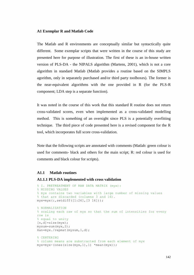
142
A1 Exemplar R and Matlab Code
The Matlab and R environments are conceptually similar but syntactically quite
different. Some exemplar scripts that were written in the course of this study are
presented here for purpose of illustration. The first of these is an in-house written
version of PLS-DA - the NIPALS algorithm (Martens, 2001), which is not a core
algorithm in standard Matlab (Matlab provides a routine based on the SIMPLS
agorithm, only in separately purchased and/or third party toolboxes). The former is
the near-equivalent algorithms with the one provided in R (for the PLS-R
component; LDA step is a separate function).
It was noted in the course of this work that this standard R routine does not return
cross-validated scores, even when implemented as a cross-validated modelling
method. This is something of an oversight since PLS is a potentially overfitting
technique. The third piece of code presented here is a revised component for the R
tool, which incorporates full score cross-validation.
Note that the following scripts are annotated with comments (Matlab: green colour is
used for comments- black and others for the main script; R: red colour is used for
comments and black colour for scripts).
A1.1 Matlab routines
A1.1.1 PLS-DA implemented with cross validation
% I. PRETREATMENT OF RAW DATA MATRIX (myx):
% MISSING VALUES
% myx contains two variables with large number of missing values
% that are discarded (columns 3 and 16).
myx=myx(:,setdiff([1:26],[3 16]));
% NORMALIZATION
% scaling each raw of myx so that the sum of intensities for every
row is
% equal to unity
[n,d]=size(myx);
mysum=sum(myx,2);
Xan=myx./repmat(mysum,1,d);
% CENTERING
% column means are substracted from each element of myx
myx=myx-(ones(size(myx,1),1) *mean(myx));
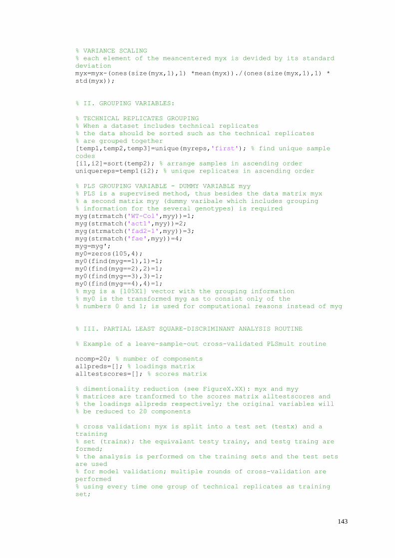
143
% VARIANCE SCALING
% each element of the meancentered myx is devided by its standard
deviation
myx=myx-(ones(size(myx,1),1) *mean(myx))./(ones(size(myx,1),1) *
std(myx));
% II. GROUPING VARIABLES:
% TECHNICAL REPLICATES GROUPING
% When a dataset includes technical replicates
% the data should be sorted such as the technical replicates
% are grouped together
[temp1,temp2,temp3]=unique(myreps,'first'); % find unique sample
codes
[i1,i2]=sort(temp2); % arrange samples in ascending order
uniquereps=temp1(i2); % unique replicates in ascending order
% PLS GROUPING VARIABLE - DUMMY VARIABLE myy
% PLS is a supervised method, thus besides the data matrix myx
% a second matrix myy (dummy varibale which includes grouping
% information for the several genotypes) is required
myg(strmatch('WT-Col',myy))=1;
myg(strmatch('act1',myy))=2;
myg(strmatch('fad2-1',myy))=3;
myg(strmatch('fae',myy))=4;
myg=myg';
my0=zeros(105,4);
my0(find(myg==1),1)=1;
my0(find(myg==2),2)=1;
my0(find(myg==3),3)=1;
my0(find(myg==4),4)=1;
% myg is a [105X1] vector with the grouping information
% my0 is the transformed myg as to consist only of the
% numbers 0 and 1; is used for computational reasons instead of myg
% III. PARTIAL LEAST SQUARE-DISCRIMINANT ANALYSIS ROUTINE
% Example of a leave-sample-out cross-validated PLSmult routine
ncomp=20; % number of components
allpreds=[]; % loadings matrix
alltestscores=[]; % scores matrix
% dimentionality reduction (see FigureX.XX): myx and myy
% matrices are tranformed to the scores matrix alltestscores and
% the loadings allpreds respectively; the original variables will
% be reduced to 20 components
% cross validation: myx is split into a test set (testx) and a
training
% set (trainx); the equivalant testy trainy, and testg traing are
formed;
% the analysis is performed on the training sets and the test sets
are used
% for model validation; multiple rounds of cross-validation are
performed
% using every time one group of technical replicates as training
set;
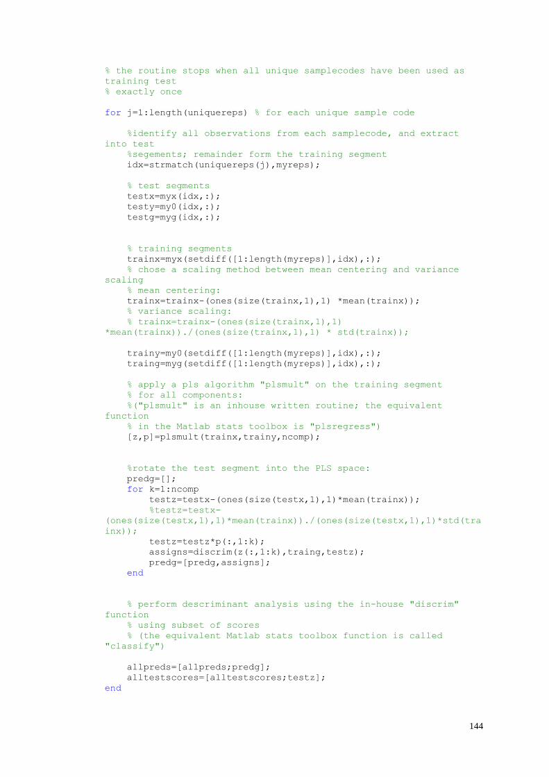
144
% the routine stops when all unique samplecodes have been used as
training test
% exactly once
for j=1:length(uniquereps) % for each unique sample code
%identify all observations from each samplecode, and extract
into test
%segements; remainder form the training segment
idx=strmatch(uniquereps(j),myreps);
% test segments
testx=myx(idx,:);
testy=my0(idx,:);
testg=myg(idx,:);
% training segments
trainx=myx(setdiff([1:length(myreps)],idx),:);
% chose a scaling method between mean centering and variance
scaling
% mean centering:
trainx=trainx-(ones(size(trainx,1),1) *mean(trainx));
% variance scaling:
% trainx=trainx-(ones(size(trainx,1),1)
*mean(trainx))./(ones(size(trainx,1),1) * std(trainx));
trainy=my0(setdiff([1:length(myreps)],idx),:);
traing=myg(setdiff([1:length(myreps)],idx),:);
% apply a pls algorithm "plsmult" on the training segment
% for all components:
%("plsmult" is an inhouse written routine; the equivalent
function
% in the Matlab stats toolbox is "plsregress")
[z,p]=plsmult(trainx,trainy,ncomp);
%rotate the test segment into the PLS space:
predg=[];
for k=1:ncomp
testz=testx-(ones(size(testx,1),1)*mean(trainx));
%testz=testx-
(ones(size(testx,1),1)*mean(trainx))./(ones(size(testx,1),1)*std(tra
inx));
testz=testz*p(:,1:k);
assigns=discrim(z(:,1:k),traing,testz);
predg=[predg,assigns];
end
% perform descriminant analysis using the in-house "discrim"
function
% using subset of scores
% (the equivalent Matlab stats toolbox function is called
"classify")
allpreds=[allpreds;predg];
alltestscores=[alltestscores;testz];
end
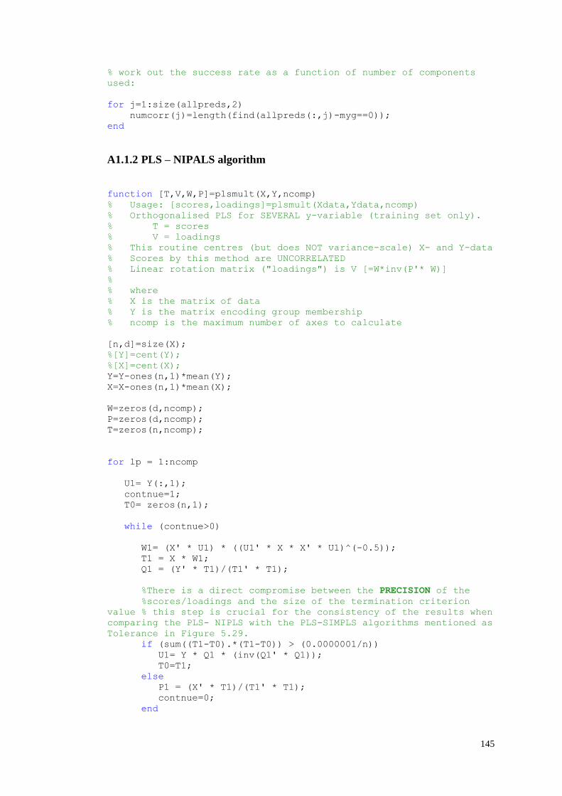
145
% work out the success rate as a function of number of components
used:
for j=1:size(allpreds,2)
numcorr(j)=length(find(allpreds(:,j)-myg==0));
end
A1.1.2 PLS – NIPALS algorithm
function [T,V,W,P]=plsmult(X,Y,ncomp)
% Usage: [scores,loadings]=plsmult(Xdata,Ydata,ncomp)
% Orthogonalised PLS for SEVERAL y-variable (training set only).
% T = scores
% V = loadings
% This routine centres (but does NOT variance-scale) X- and Y-data
% Scores by this method are UNCORRELATED
% Linear rotation matrix ("loadings") is V [=W*inv(P'* W)]
%
% where
% X is the matrix of data
% Y is the matrix encoding group membership
% ncomp is the maximum number of axes to calculate
[n,d]=size(X);
%[Y]=cent(Y);
%[X]=cent(X);
Y=Y-ones(n,1)*mean(Y);
X=X-ones(n,1)*mean(X);
W=zeros(d,ncomp);
P=zeros(d,ncomp);
T=zeros(n,ncomp);
for lp = 1:ncomp
U1= Y(:,1);
contnue=1;
T0= zeros(n,1);
while (contnue>0)
W1= (X' * U1) * ((U1' * X * X' * U1)^(-0.5));
T1 = X * W1;
Q1 = (Y' * T1)/(T1' * T1);
%There is a direct compromise between the PRECISION of the
%scores/loadings and the size of the termination criterion
value % this step is crucial for the consistency of the results when
comparing the PLS- NIPLS with the PLS-SIMPLS algorithms mentioned as
Tolerance in Figure 5.29.
if (sum((T1-T0).*(T1-T0)) > (0.0000001/n))
U1= Y * Q1 * (inv(Q1' * Q1));
T0=T1;
else
P1 = (X' * T1)/(T1' * T1);
contnue=0;
end
146
end
T(:,lp)=T1;
W(:,lp)=W1;
P(:,lp)=P1;
X= X - (T1 * P1');
Y= Y - (T1 * Q1');
end
V = W * inv(P' * W);
A1.2 R routines
A1.2.1 PLS-DA implemented with cross validation
# DATA PREPARATION AND PRETREATMENT IN R
getwd()
list.files()
library(pls)
oliveoil<-read.table(file.choose(), header=T, fill=TRUE)
attach(oliveoil)
greece<-oliveoil[1:10,]
italy<-oliveoil[11:27,]
portugal<-oliveoil[28:35,]
spain<-oliveoil[36:60,]
# creating a vector of responses (binary)
y<-cbind(c(rep(1, 10), rep(0,50)), c(rep(0,10), rep(1, 17), rep(0,
33)),
c(rep(0, 27), rep(1,8), rep(0,25)), c(rep(0, 35), rep(1, 25)))
# rownames, colnames
rownames(y)<-c(1:60)
colnames(y)<-c("Greece", "Italy", "Portugal", "Spain")
# creating a test set
ooTest.all<-rbind(greece[1:2, ], italy[1:3, ], portugal[1, ],
spain[1:5, ])
ooTest<-as.matrix(ooTest.all[,-c(1:2)])
# creating a training set
X<-as.matrix(rbind(greece[-(1:2), 3:ncol(greece)], italy[-(1:3),
3:ncol(italy)],
portugal[-1, 3:ncol(portugal) ], spain[-(1:5), 3:ncol(spain) ]))
test.rows<-c(1:2, 11:13, 28, 36:40)
Y<-as.matrix(y[-test.rows,])
147
# the training data frame
ooTrain<-data.frame(Y=I(Y), X=I(X))
# running pls
ooTrain.pls<-plsr(Y ~ X, data=ooTrain, validation="LOO")
# change colours
rainbow<-rainbow(4)
cols<- c(rep(rainbow[1], 10), rep(rainbow[2], 17),
rep(rainbow[3],8), rep(rainbow[4],25))
trainCols<-cols[-test.rows]
# mean centering
X.cent<-apply(ooTrain$X, 2, meanCent)
meanCent<-function(x){
newX<-x-mean(x)
}
Y.cent<-apply(ooTrain$Y, 2, meanCent)
# centered training data
train.cent<-data.frame(Y=I(Y.cent), X=I(X.cent))
# PLS on centered data
train.c.pls<-plsr(Y~X, data=train.cent, validation="LOO",
method="oscorespls", ncomp=10)
# scores plot
plot(train.c.pls, "scores", comp=1:4, col=trainCols)
# pls on random data
x.random<-matrix(ncol=ncol(X.cent), nrow=nrow(X.cent),
data=rep(rnorm(ncol(X.cent)), nrow(X.cent)))
random.df<-data.frame(Y=I(Y.cent), X=I(x.random))
pls.rand<-plsr(Y~X, data=random.df, ncomp=4, validation="LOO",
method="oscorespls")
# VALIDATION DESIGN
# perform pls on a
ooTrain.pls<-plsr(Y ~ X, ncomp=4, data=ooTrain, method="oscorespls",
validation="LOO")
# ooTrain.pls$validation$scores
# extract scores into matrix
scoresList<-ooTrain.pls$validation$scores
scoreMat<-matrix(nrow=nrow(ooTrain), ncol=ncol(scoresList[[1]]))
rownames(scoreMat)<-rownames(ooTrain)
colnames(scoreMat)<-colnames(scoresList[[1]])
# makes a large matrix bound by rows (the rownames repeat and are
the observation IDs)
allScores<-do.call('rbind', scoresList)
148
# go through the original rownames
for (i in 1:nrow(ooTrain)){
obsID.pattern<-paste("^",rownames(ooTrain)[i],"$", sep="")
# grep the indices from the rownames of the allScores matrix
all.indices<-grep(obsID.pattern, rownames(allScores), perl=T)
# in the score Matrix, of observation i, store the average of the
scores
scoreMat[i,]<-apply(allScores[all.indices,], 2, mean)
}
# pls on random data
randData<-matrix(nrow=nrow(ooTrain$X), ncol=ncol(ooTrain$X))
randData<-apply(randData, 2, rnorm, ncol(randData))
dimnames(randData)<-dimnames(ooTrain$X)
rand.df<-data.frame(Y=I(Y), X=I(randData))
rand.pls<-plsr(Y~X, ncomp=4, data=rand.df, method="oscorespls",
validation="LOO")
# get the means of the validation scores
rand.scores<-rand.pls$validation$scores
rand.v.scores<-matrix(nrow=nrow(randData),
ncol=ncol(rand.scores[[1]]))
allRandscores<-do.call('rbind', rand.scores)
for (i in 1:nrow(randData)){
obsID.pattern<-paste("^", rownames(randData)[i], "$", sep="")
all.ind<-grep(obsID.pattern, rownames(allRandscores), perl=T)
rand.v.scores[i,]<-apply(allRandscores[all.ind,], 2, mean)
}
plot(rand.v.scores, type="p",col=trainCols)
# the algorithm is overfitting, potential pitfall of weak cross-
validation routine
A1.2.2 PLS – A1.1.2 PLS – mvrCv function
# Changes to mvrCv function of package pls to ensure that cross
validated scores are returned
(notes from July 2009)
mvrCv<-function (X, Y, ncomp, method = pls.options()$mvralg, scale =
FALSE,
segments = 10, segment.type = c("random", "consecutive",
"interleaved"), length.seg, jackknife = FALSE, trace =
FALSE,
...)
{
Y <- as.matrix(Y)
dnX <- dimnames(X)
dnY <- dimnames(Y)
nobj <- dim(X)[1]
npred <- dim(X)[2]
nresp <- dim(Y)[2]
149
if (!is.logical(scale) || length(scale) != 1)
stop("'scale' must be 'TRUE' or 'FALSE'")
if (is.list(segments)) {
if (is.null(attr(segments, "type")))
attr(segments, "type") <- "user supplied"
}
else {
if (missing(length.seg)) {
segments <- cvsegments(nobj, k = segments, type =
segment.type)
}
else {
segments <- cvsegments(nobj, length.seg = length.seg,
type = segment.type)
}
}
ncomp <- min(ncomp, nobj - max(sapply(segments, length)) -
1)
method <- match.arg(method, c("kernelpls", "widekernelpls",
"simpls", "oscorespls", "svdpc"))
fitFunc <- switch(method, kernelpls = kernelpls.fit,
widekernelpls = widekernelpls.fit,
simpls = simpls.fit, oscorespls = oscorespls.fit, svdpc =
svdpc.fit)
adj <- matrix(0, nrow = nresp, ncol = ncomp)
cvPred <- pred <- array(0, dim = c(nobj, nresp, ncomp))
# scores <- array(0, dim=c((nobj-1), ncomp, length(segments)))
# cvScores <-array(0, dim=c(nobj, ncomp, length(segments)))
cvScores<-list(length=length(segments))
if (jackknife)
cvCoef <- array(dim = c(npred, nresp, ncomp,
length(segments)))
if (trace)
cat("Segment: ")
for (n.seg in 1:length(segments)) {
if (trace)
cat(n.seg, "")
seg <- segments[[n.seg]]
Xtrain <- X[-seg, ]
if (scale) {
ntrain <- nrow(Xtrain)
sdtrain <- sqrt(colSums((Xtrain - rep(colMeans(Xtrain),
each = ntrain))^2)/(ntrain - 1))
if (any(abs(sdtrain) < .Machine$double.eps^0.5))
warning("Scaling with (near) zero standard
deviation")
Xtrain <- Xtrain/rep(sdtrain, each = ntrain)
}
fit <- fitFunc(Xtrain, Y[-seg, ], ncomp, stripped = FALSE,
...)
cvScores[[n.seg]]<-I(fit$scores)
if (jackknife)
cvCoef[, , , n.seg] <- fit$coefficients
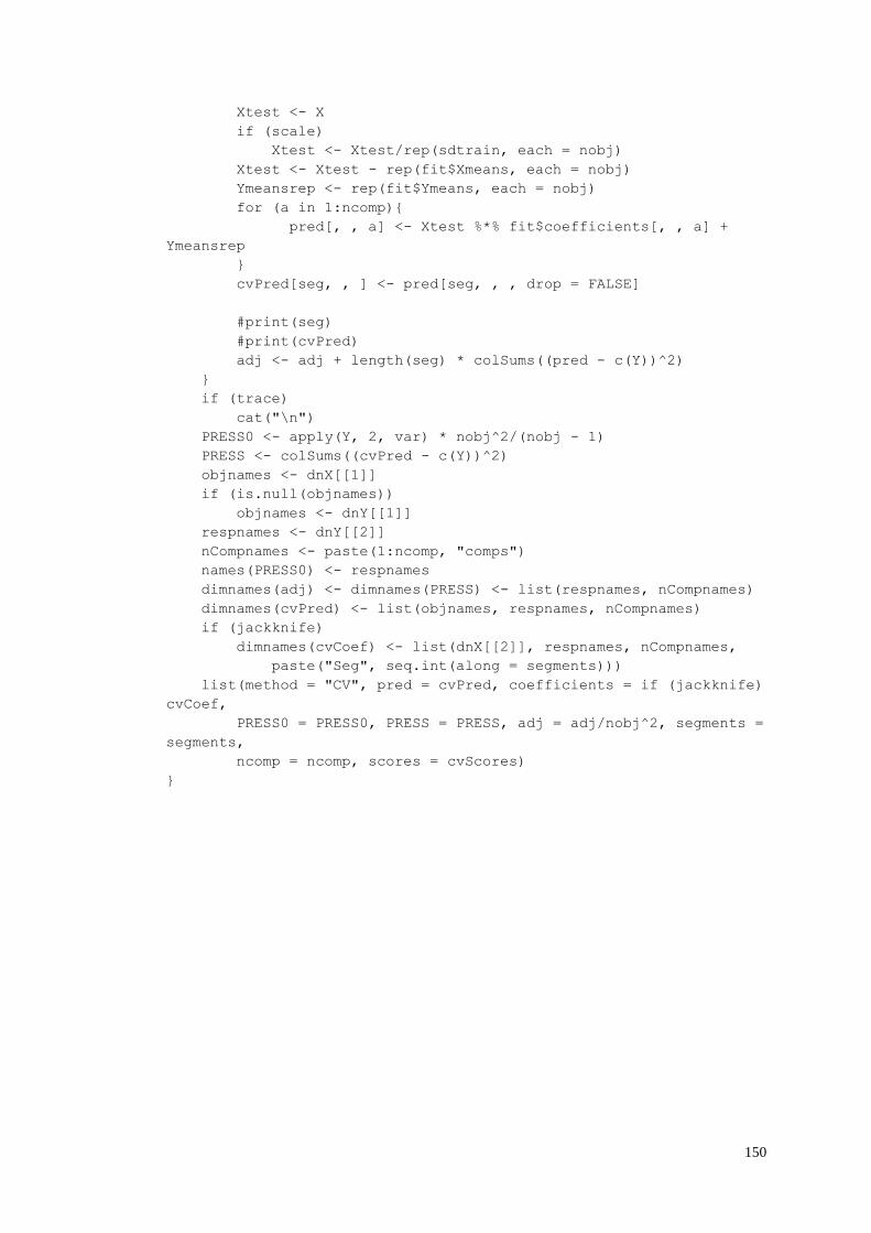
150
Xtest <- X
if (scale)
Xtest <- Xtest/rep(sdtrain, each = nobj)
Xtest <- Xtest - rep(fit$Xmeans, each = nobj)
Ymeansrep <- rep(fit$Ymeans, each = nobj)
for (a in 1:ncomp){
pred[, , a] <- Xtest %*% fit$coefficients[, , a] +
Ymeansrep
}
cvPred[seg, , ] <- pred[seg, , , drop = FALSE]
#print(seg)
#print(cvPred)
adj <- adj + length(seg) * colSums((pred - c(Y))^2)
}
if (trace)
cat("\n")
PRESS0 <- apply(Y, 2, var) * nobj^2/(nobj - 1)
PRESS <- colSums((cvPred - c(Y))^2)
objnames <- dnX[[1]]
if (is.null(objnames))
objnames <- dnY[[1]]
respnames <- dnY[[2]]
nCompnames <- paste(1:ncomp, "comps")
names(PRESS0) <- respnames
dimnames(adj) <- dimnames(PRESS) <- list(respnames, nCompnames)
dimnames(cvPred) <- list(objnames, respnames, nCompnames)
if (jackknife)
dimnames(cvCoef) <- list(dnX[[2]], respnames, nCompnames,
paste("Seg", seq.int(along = segments)))
list(method = "CV", pred = cvPred, coefficients = if (jackknife)
cvCoef,
PRESS0 = PRESS0, PRESS = PRESS, adj = adj/nobj^2, segments =
segments,
ncomp = ncomp, scores = cvScores)
}

151
APPENDIX A2:
SUPPLEMENTARY MATERIAL FOR CHAPTER 4
Table 4.4
Table 4.5
Table 4.6
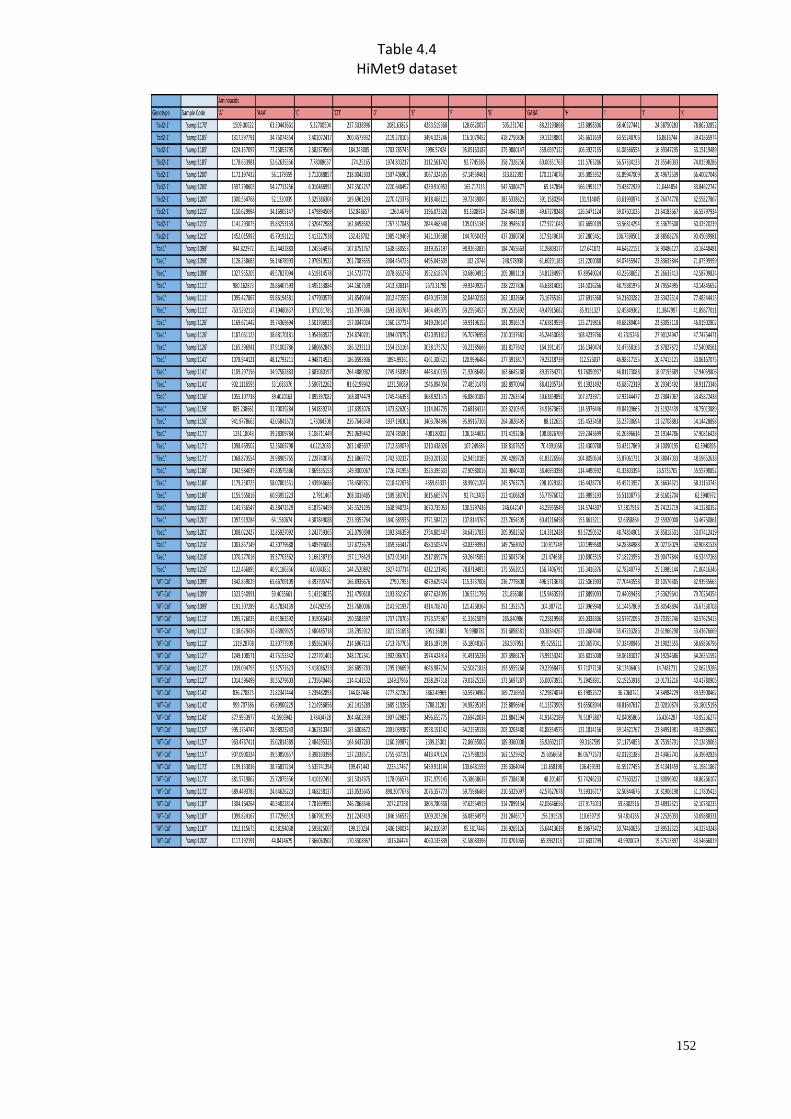
152
Table 4.4 HiMet9 dataset
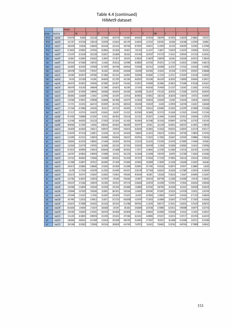
153
Aminoacids
Genotype Sample Code 'A' 'AAA' 'C' 'CIT' 'D' 'E' 'F' 'G' 'GABA' 'H' 'I' 'J' 'K'
'WT‐Col' 'sampl1202' 919.4327108 50.668246 2.022411286 102.7034449 1649.977764 3146.585851 68.96561825 239.7852546 70.88247995 105.7935301 42.20635766 22.76880425 47.0027225
'WT‐Col' 'sampl1202' 1232.753877 44.47871608 2.289011328 170.0878708 2135.836118 4485.157987 82.34485764 313.2705247 82.09470031 138.439664 56.58214986 21.50578596 56.5868055
'WT‐Col' 'sampl1217' 1006.566786 20.6945386 6.530006305 160.0414624 1626.513019 3493.974602 88.70299247 159.6563571 110.1948378 100.135339 64.08410978 15.03293001 61.24739849
'WT‐Col' 'sampl1217' 871.3684262 42.09598415 2.391794565 226.3898415 1205.106056 3169.48273 72.83712014 155.1322477 57.2685677 77.00401359 42.22634379 15.90184645 49.0162556
'fad2‐1' 'sampl1097' 1172.634374 36.19416189 3.829122386 82.0649127 1392.588684 3605.81363 87.69716483 228.9105507 87.45713728 117.4614121 50.99599169 35.43711029 64.24029361
'fad2‐1' 'sampl1097' 1250.98016 43.10383932 3.506142032 151.849199 1767.786773 2634.92781 81.76982145 237.4040278 52.09803798 160.534052 56.42021004 26.90787119 57.26850419
'fad2‐1' 'sampl1097' 1029.535342 63.75938968 2.530871393 115.244666 1953.891126 3159.909893 68.29889236 202.9572065 397.6697213 112.1713076 46.21961925 15.55690841 63.40661718
'fad2‐1' 'sampl1125' 1166.498078 46.29023305 5.505788598 235.7459879 1804.973848 4609.894224 78.28785968 308.5754125 43.43348938 126.2627657 57.67251652 19.39352608 67.18879802
'fad2‐1' 'sampl1125' 1489.441998 57.86323478 5.778543337 283.103662 2040.03946 4034.681848 118.0292969 606.8758302 65.9632465 183.705348 67.17897914 20.98255875 84.58666088
'fad2‐1' 'sampl1125' 1234.61968 38.02307279 5.947076962 291.7286602 1987.155241 3144.498147 78.03879496 403.4364067 111.7223191 122.6273117 63.70324979 23.14011589 54.10301692
'fad2‐1' 'sampl1140' 1376.0254 32.92723658 4.43116835 196.4862926 2021.270955 3401.253647 66.40203379 299.5319003 438.4116979 166.3876022 57.30982859 29.69640246 81.03495271
'fad2‐1' 'sampl1140' 1668.392743 48.42000155 5.299359854 320.7906897 2834.329677 4754.626021 92.53045712 476.8298009 620.3468665 204.5080153 78.73199969 34.78523488 94.93146257
'fad2‐1' 'sampl1140' 1580.954783 42.58113639 5.968485948 215.7208406 2654.060718 4010.35996 126.7543343 494.8357683 770.0440299 225.5110377 72.20318437 23.12628201 104.7545563
'fad2‐1' 'sampl1155' 1162.603872 40.74295584 2.548904845 164.8638663 1483.043454 3645.650033 108.6428586 258.1220174 47.95115281 106.0037601 67.27258248 25.94077051 68.62945454
'fad2‐1' 'sampl1155' 1089.389923 31.66463099 3.17189107 161.4879406 1343.519873 2229.784135 88.49398726 229.7089321 29.68157183 100.6637654 55.39304729 18.7927333 44.87368407
'fad2‐1' 'sampl1155' 1174.629603 43.78189151 5.678992086 156.4890398 1983.738066 4140.037767 101.1862246 299.8393243 44.26362429 123.434687 59.33362439 28.1865349 63.68910336
'fad2‐1' 'sampl1170' 1227.37555 53.01187631 4.684217523 205.9387697 1861.370016 3869.901032 109.8223589 376.9019479 55.410933 113.8790078 53.42877683 15.56160517 55.66585689
'WT‐Col' 'sampl1217' 1172.752636 43.17948638 2.410541992 189.105129 1634.723222 4204.087851 81.17741597 203.0013312 69.35589441 105.3240922 61.62297097 18.73490938 67.82102808
'fad2‐1' 'sampl1170' 1227.131127 41.92278714 5.816362979 167.8616811 1258.82097 2319.103222 89.38738549 338.7684095 38.27472278 101.4554693 56.17003255 23.05454032 47.21571843
'act1' 'sampl1096' 997.1447982 37.89680048 3.671520367 119.391423 2068.786543 5578.022356 105.2135012 189.2290271 121.5484433 95.18434078 56.03769113 23.46876964 51.35780729
'act1' 'sampl1096' 1111.874384 40.66023953 2.931321226 127.5938726 1872.302581 4531.148324 99.81399534 206.2745885 105.5565106 89.95094973 56.87675081 16.33774529 47.40311495
'act1' 'sampl1096' 989.0095834 34.17076491 3.14596236 90.88465106 1894.484502 4860.640038 90.90729779 192.802911 104.5131839 96.04029413 48.85025337 20.11985551 47.39969108
'act1' 'sampl1110' 1106.449709 46.43564334 3.746452171 93.06981791 1749.964578 3439.836718 96.24667483 303.3498101 78.17645226 99.06547433 65.62487467 25.33152758 48.94371177
'act1' 'sampl1110' 873.3667814 40.57321108 2.252808171 122.2033581 1358.11109 3644.690108 71.88600276 241.1642223 54.90261278 96.33004261 39.48773938 17.29880199 43.79374926
'act1' 'sampl1110' 1221.509495 65.31741212 2.524806759 126.9036685 2048.368104 5180.633575 99.58797641 272.1596272 115.7918625 130.8160672 55.04763407 19.58898863 57.95056296
'act1' 'sampl1124' 1230.869501 48.10107503 3.748830561 137.3148426 2169.582505 3902.295164 122.5623119 355.1612035 97.55159504 126.1697382 60.72389935 17.47446605 59.3596206
'act1' 'sampl1124' 1216.583204 25.56157799 1.545979352 146.2286286 2248.123362 3827.292016 92.60325205 268.4570298 151.320048 103.9228844 56.03809581 26.4164135 47.03870966
'act1' 'sampl1124' 997.3205147 46.99999544 4.744933134 86.95864548 1473.300488 3867.900312 91.7329772 221.6969281 112.2373897 91.52336854 47.53475136 33.04724207 46.41195992
'act1' 'sampl1139' 1138.374677 66.93886193 4.548879928 157.4698496 2012.99313 5083.122945 93.41282448 323.2290998 74.00373599 103.840799 62.52573809 27.15818526 64.42203846
'act1' 'sampl1139' 1118.753223 48.06856619 7.374204692 170.6343889 1985.925341 3921.342369 109.7015975 267.9501854 55.77134193 107.9380541 59.62611363 31.06911425 59.03920222
'act1' 'sampl1139' 1213.708839 45.50809774 2.897782227 180.4694967 1747.239596 3973.089693 109.7809332 299.6398009 117.4809455 101.3333964 67.63665968 25.35582875 60.4661488
'act1' 'sampl1154' 1045.801735 42.50088422 6.328845802 137.0184165 1926.768549 4521.609386 95.09368741 293.7734961 94.47813261 95.36993774 59.0935477 18.12888687 61.842303
'act1' 'sampl1154' 1101.8766 51.17755436 4.782267958 161.1535915 1916.618905 4847.630271 92.58151789 250.7779628 66.45820192 102.0010585 62.23728887 14.32007544 56.15836054
'act1' 'sampl1154' 1010.922732 35.45077471 2.970189437 125.4960351 1778.490145 4799.816901 89.59641044 186.508675 72.36140558 97.03061918 57.2041407 18.94289491 61.19242967
'act1' 'sampl1169' 1232.576852 56.19602379 3.102693518 144.3790274 1978.18496 4700.646822 110.5984471 238.9613319 88.82773964 113.2528685 46.24505894 18.7691346 55.48813961
'act1' 'sampl1169' 1029.821397 33.72216682 1.269590744 125.6720653 1566.593313 3097.571782 81.69260238 210.6397934 161.6639396 76.55530913 43.3706186 24.06821835 46.00034828
'act1' 'sampl1169' 1240.392806 31.26605449 1.932025636 152.9236784 2290.314602 4914.696085 123.0808939 263.9752841 40.08775843 106.4520438 66.3233104 29.60935508 60.62823199
'act1' 'sampl1184' 1278.089448 41.87765059 7.950361894 258.309622 2864.760132 5183.951842 111.8443934 399.6974807 69.73566972 130.5022245 52.43747298 29.5263021 51.69157949
'act1' 'sampl1184' 1037.824469 21.41013672 1.111700391 194.2626037 2018.568704 3776.436751 100.415907 283.7986045 113.9800593 72.40447357 53.26543019 26.77217393 40.58683304
'act1' 'sampl1184' 1491.749691 71.22092192 3.574098113 235.605572 2672.327324 6063.858788 141.0547397 477.3266516 101.9098639 129.0269557 63.77746707 25.71240354 63.40160036
'act1' 'sampl1199' 1041.666741 39.73506883 3.462362813 104.3162263 1658.759532 4151.078866 98.89793431 211.2626785 84.86471767 92.72613611 56.69189101 19.37615299 68.83607333
'act1' 'sampl1199' 865.4166429 23.9442894 1.772100274 130.8428208 1367.40567 3403.50305 92.96682048 182.8716366 63.37988092 82.01295131 59.09693898 14.96697779 62.05277418
'act1' 'sampl1199' 1109.414991 37.66634674 4.129726921 106.8764736 1945.460269 4432.881965 127.685114 269.0856873 86.41498035 93.61833668 60.1951563 33.1763023 81.50240137
'act1' 'sampl1214' 1251.612655 46.10883391 8.598992784 133.5107026 2239.163553 4579.720836 96.25102421 244.6989853 48.70163271 124.8202154 55.50751717 18.92237044 46.44415376
'act1' 'sampl1214' 1188.680618 44.89618311 4.013176849 112.9656118 1995.263828 4308.473932 95.24444076 217.7959677 98.0535247 108.1448489 59.16196384 23.40227511 60.19315884
'act1' 'sampl1214' 1004.224004 50.28392801 2.728283696 149.9233164 1898.860189 4642.479493 73.46799725 226.460218 79.00466953 92.26971862 48.48759336 20.77898088 53.84945622
Table 4.4 (continued) HiMet9 dataset
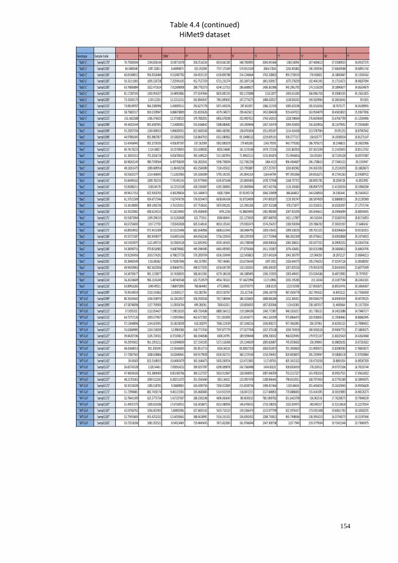
154
Genotype Sample Code 'L' 'N' 'ORN' 'P' 'Q' 'R' 'S' 'T' 'V' 'W' 'Y'
'fad2‐1' 'sampl1170' 70.75006504 1194.826144 10.90715478 358.2516234 8319.662185 348.7000995 2040.491466 1383.56094 247.4404612 37.55089923 34.09107276
'fad2‐1' 'sampl1185' 64.3480548 1097.32851 8.46994875 325.192298 7757.175349 574.9213169 2064.57826 1250.401862 196.1929545 27.66639588 29.68951742
'fad2‐1' 'sampl1185' 60.81308012 956.9226484 9.312087782 334.4531133 6150.892788 214.1246664 1762.328852 993.1736519 176.920822 24.18830467 33.13334162
'fad2‐1' 'sampl1185' 50.32111081 1005.520728 7.255941435 452.7527259 6721.231374 265.2697134 1861.030917 1075.578259 192.4641391 31.17134271 38.98207094
'fad2‐1' 'sampl1200' 63.76806884 1022.471614 7.012698908 288.7792373 6244.117313 286.6688027 1406.361986 945.2961792 174.1516109 29.18840677 34.06334679
'fad2‐1' 'sampl1200' 81.17287243 1303.954257 10.48953882 377.0247664 8025.892155 302.1170088 2110.2877 1405.613283 266.0961726 35.03083155 45.15611825
'fad2‐1' 'sampl1200' 73.33265175 1159.12201 12.21512311 342.8944547 7061.809635 247.2774275 1488.420527 1138.834242 194.5629964 42.36016441 39.0101
'fad2‐1' 'sampl1215' 73.08149707 964.2385996 5.430093511 293.6271778 5071.459226 287.651057 1586.212193 1005.623196 185.5516256 30.7675177 34.26189955
'fad2‐1' 'sampl1215' 58.75802517 850.5339947 8.886078899 235.8335626 4579.248272 290.4625611 1452.084638 919.4247023 163.9504079 30.45818023 25.93677836
'fad2‐1' 'sampl1215' 116.1662588 1186.374625 12.37338525 379.7802051 6902.678298 352.9007621 1764.542013 1228.598669 276.6630604 53.67667709 41.12504906
'fae1' 'sampl1098' 49.34202544 891.6587691 7.214085851 555.6368642 5588.880682 134.2839696 1367.524476 1094.453003 156.2629816 28.11679052 37.29246083
'fae1' 'sampl1098' 55.29207256 1240.069015 5.896009351 823.5605338 8481.482981 158.8763004 1551.093347 1214.424438 213.5787964 29.951252 18.87967642
'fae1' 'sampl1098' 44.97881045 855.9867857 10.53820592 510.8647915 6312.080062 95.19488132 1219.695191 939.2777217 158.635777 24.10508334 20.81275147
'fae1' 'sampl1111' 52.42456943 902.3729335 4.926397397 537.262599 5952.890329 179.405285 1243.79293 943.7770282 186.7076272 30.2248813 20.20622906
'fae1' 'sampl1111' 60.74176223 1114.34827 10.25769055 553.1698282 8026.54848 161.3176186 1479.172324 1101.862819 207.3615269 21.21420453 20.85113762
'fae1' 'sampl1111' 41.30355313 755.2026719 9.056700563 395.1499223 5111.807876 71.99923112 1135.491874 751.9934816 154.591833 18.71295328 18.09737087
'fae1' 'sampl1126' 60.98262143 980.7339564 6.407768249 556.2822631 5596.758034 212.7381258 1064.4123 906.4364607 196.1708615 27.73465122 30.1353947
'fae1' 'sampl1126' 48.18261475 1089.689954 11.86430258 463.2568389 7130.435021 123.7993887 1257.257937 1030.802982 194.3633392 31.25136359 26.18828673
'fae1' 'sampl1126' 50.91625277 1114.460645 7.111815965 535.3266384 5793.192191 141.8041314 1164.64704 997.3931066 169.8316271 34.17341263 22.04589722
'fae1' 'sampl1141' 55.66494162 1009.782155 7.741491143 525.9779465 6145.871648 125.8693405 1478.727048 1168.737372 180.8931781 28.2036728 41.8552992
'fae1' 'sampl1141' 55.06386211 1030.04178 16.22152538 428.2356967 6192.308065 155.9699944 1457.432766 1126.265683 208.8947579 21.41356554 20.24960284
'fae1' 'sampl1141' 49.94117552 822.9350765 4.365290634 555.1469473 4500.71894 87.01592724 1046.259699 846.664812 144.5268924 24.5381441 18.25454522
'fae1' 'sampl1156' 61.37521509 924.6717546 7.627476736 576.9254473 6638.841434 92.07524699 1747.893207 1129.392747 180.5874929 32.88808015 29.21292969
'fae1' 'sampl1156' 53.34148085 809.1492736 3.761191911 427.7538161 5874.991201 115.2991206 1297.352188 978.271877 153.3526551 24.05202937 27.17571744
'fae1' 'sampl1156' 63.35220581 838.6134212 9.126139463 676.4584693 5976.2236 91.88659693 1381.980385 1047.923295 245.6546611 26.59466094 26.88344041
'fae1' 'sampl1171' 65.91872064 1249.296315 10.31263608 621.772411 8584.80443 221.1276926 1807.068765 1421.117897 243.532434 27.01820743 28.81716953
'fae1' 'sampl1171' 60.67256693 1017.27759 7.055455838 605.5148141 8010.135341 179.9302475 1574.254257 1300.930394 229.7866702 37.58101937 27.6484242
'fae1' 'sampl1171' 43.89324932 972.4515309 8.515225496 682.6540906 6608.612443 158.0484795 1303.576431 1099.558195 199.7011321 30.82046654 19.92163315
'fae1' 'sampl1186' 45.55715587 983.9439077 9.624051436 404.6562244 5734.229543 108.2295509 1317.753948 986.3632309 185.9736611 29.69928808 29.24734923
'fae1' 'sampl1186' 64.51925875 1121.695715 10.35829128 512.6953932 6559.165455 143.1788598 1400.838416 1065.586011 230.5677252 24.09092252 33.02647236
'fae1' 'sampl1186' 54.38390731 970.8316982 9.668790682 449.2984385 6463.495903 177.8756366 1411.191857 1076.426831 183.0131988 28.36606812 25.68424745
'fae1' 'sampl1201' 59.92260456 1033.574291 8.788157726 570.2859704 6336.354949 122.5458823 1357.643164 1043.383797 215.984293 28.2872127 25.06846213
'fae1' 'sampl1201' 50.38483549 1153.86362 9.792857846 461.557893 7927.46065 223.6736434 1597.3921 1326.644275 195.2746252 37.01547126 31.08188292
'fae1' 'sampl1201' 49.94359063 962.5622056 8.906467911 498.5173291 6234.691709 110.1350241 1495.439187 1057.825526 179.9553578 23.84144355 23.60775599
'fae1' 'sampl1216' 54.34793677 981.1150877 10.74260635 586.0411961 6279.184158 146.1889405 1266.153035 1003.449421 223.0264186 26.48719902 29.7979507
'fae1' 'sampl1216' 56.26158609 906.1535249 5.487403548 632.7519579 4954.745321 97.14672994 1117.10906 1035.195285 213.16354 23.31877594 28.22432101
'fae1' 'sampl1216' 63.89916265 1049.49521 7.886972893 768.864483 6772.89601 110.9733775 1308.0135 1223.91598 217.8502671 26.89134741 30.10646367
'WT‐Col' 'sampl1099' 76.99144019 1510.191862 21.8345117 451.082784 8519.250767 251.417246 1396.140739 987.4504778 242.7491622 34.8453122 61.73364658
'WT‐Col' 'sampl1099' 80.35343642 1436.918973 16.13613917 558.2920326 7417.586944 186.3236605 1688.066286 1152.365921 269.0566179 36.84565924 30.40739125
'WT‐Col' 'sampl1099' 67.58748096 1157.793905 11.05926764 499.289261 7000.62021 120.8056055 1657.820366 1124.63383 238.1607017 31.4695664 35.13172924
'WT‐Col' 'sampl1112' 57.9293332 1132.054427 7.198126105 409.7354586 6889.264113 119.1084596 1340.772987 946.5501017 181.7786131 24.34553086 24.79487577
'WT‐Col' 'sampl1112' 64.72757126 1093.577857 7.193919463 462.6717001 7211.853093 123.4536771 1461.163299 975.8866473 220.9180655 21.19584061 30.86862945
'WT‐Col' 'sampl1112' 57.13648896 1144.625091 10.18158209 418.182079 7368.113539 107.1046216 1336.858171 957.3662891 206.337061 24.82301221 21.78984021
'WT‐Col' 'sampl1127' 55.62684985 1234.150039 12.9983588 418.7717434 7597.877779 177.0277458 1247.373138 1039.743919 189.5058126 29.94047752 27.18830275
'WT‐Col' 'sampl1127' 39.84207196 1105.724531 8.371038117 360.3346586 6500.24795 189.9298448 1098.258332 968.0229492 179.9721137 21.80225423 24.42624068
'WT‐Col' 'sampl1127' 49.29545815 961.1953121 6.510948609 327.1541505 5171.516308 135.1346639 1085.826807 745.0536602 158.399843 16.08828191 19.07263022
'WT‐Col' 'sampl1142' 48.42648313 831.350194 12.55434605 281.8512713 4334.36318 85.00027318 1060.052873 701.3930603 131.9959571 15.82069282 17.96818572
'WT‐Col' 'sampl1142' 57.72067563 1008.628866 10.62640441 459.9179928 6350.367215 360.1219169 1150.294452 820.4058875 205.2339947 19.58006118 21.97020864
'WT‐Col' 'sampl1142' 39.45605 823.5168915 10.64065479 365.1646473 5650.269554 123.4713065 1117.69763 605.3415322 130.4710336 20.8891054 16.90587209
'WT‐Col' 'sampl1157' 56.82743528 1128.54461 7.050914252 399.9257397 6290.009878 242.7360498 1434.00225 928.8356919 178.250512 24.97372106 16.78155744
'WT‐Col' 'sampl1157' 47.46036326 931.3809405 8.851365766 380.1127257 5010.313067 128.5608591 1087.046359 753.2117227 141.4782324 18.95917521 17.05614022
'WT‐Col' 'sampl1157' 48.21703363 1069.512242 8.282511075 351.5565469 5831.36632 125.0957478 1188.966442 798.6510551 168.7973454 16.57701589 16.38945075
'WT‐Col' 'sampl1172' 50.35218328 1385.518781 9.30689803 420.4395754 7204.012809 215.8339736 1398.457464 1103.04634 201.4426016 23.26226943 24.99356628
'WT‐Col' 'sampl1172' 51.72994881 882.7433176 9.461213301 335.0600483 5114.922559 118.0472215 1127.848855 770.0886065 155.4141091 24.30159893 24.98126273
'WT‐Col' 'sampl1172' 32.78441309 625.5775734 5.417237607 288.2392248 4696.063645 88.9639218 780.1969782 651.6423709 136.962516 17.76238575 19.79046539
'WT‐Col' 'sampl1187' 51.49537275 1300.623186 17.67169551 526.3018471 8152.480926 146.6706531 1710.198255 1325.024975 240.040217 31.52119618 15.22170254
'WT‐Col' 'sampl1187' 42.03766762 1056.001992 5.84892906 427.6835142 5423.710123 139.2366474 1213.977799 922.5976417 173.0351408 19.60811763 18.16920235
'WT‐Col' 'sampl1187' 52.75950683 953.4252532 12.64550661 388.0418991 5516.331352 156.8392452 1288.733813 965.7498046 138.3954215 16.55746575 19.21597646
'WT‐Col' 'sampl1202' 53.72518206 1081.922521 8.54523469 719.4845455 7671.822005 161.9766046 1547.300738 1157.7945 219.3779504 19.72421546 23.73069375
Table 4.4 (continued) HiMet9 dataset
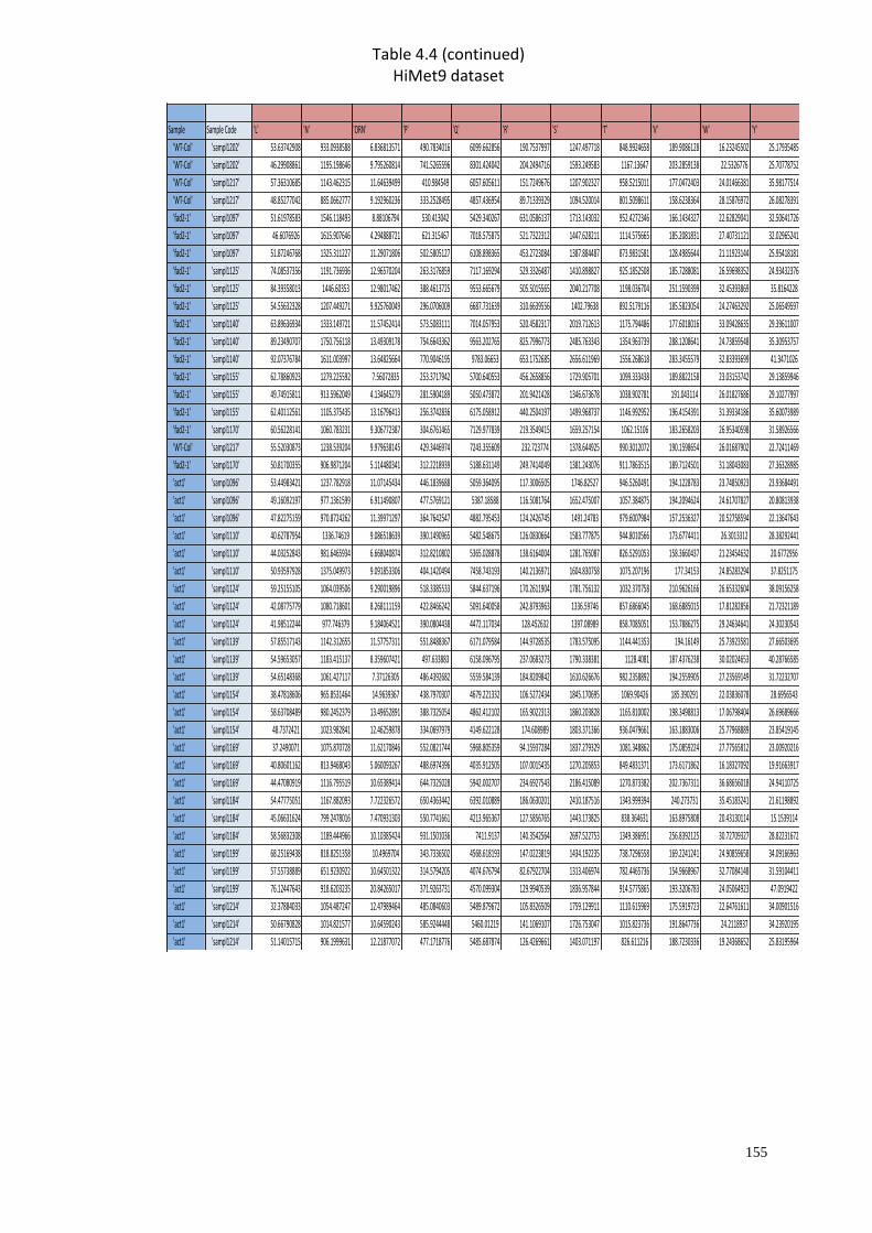
155
Sample Sample Code 'L' 'N' 'ORN' 'P' 'Q' 'R' 'S' 'T' 'V' 'W' 'Y'
'WT‐Col' 'sampl1202' 53.63742908 933.0938588 6.836813571 490.7834016 6099.662856 190.7537997 1247.497718 848.9924658 189.9086128 16.23245502 25.17935485
'WT‐Col' 'sampl1202' 46.29908861 1195.198646 9.795260814 741.5265596 8301.424042 204.2494716 1593.249583 1167.13647 203.2859138 22.5326776 25.70778752
'WT‐Col' 'sampl1217' 57.36310685 1143.462315 11.64639499 410.984549 6057.605611 151.7249676 1207.902327 958.5215011 177.0472403 24.01466381 35.98177514
'WT‐Col' 'sampl1217' 48.85277042 885.0662777 9.192960236 333.2528495 4857.436954 89.71339329 1094.520014 801.5098611 158.6238364 28.15876972 26.08278391
'fad2‐1' 'sampl1097' 51.61978583 1546.118493 8.88106794 530.413042 5429.340267 631.0586137 1713.143032 952.4272346 166.1434327 22.62829041 32.50641726
'fad2‐1' 'sampl1097' 46.6076926 1615.907646 4.294888721 621.315467 7018.575875 521.7322312 1447.628211 1114.575665 185.2081831 27.40731121 32.02965241
'fad2‐1' 'sampl1097' 51.87246768 1325.311227 11.29071806 502.5805127 6108.898365 453.2723084 1387.884487 873.9831581 128.4985644 21.11923144 25.95418181
'fad2‐1' 'sampl1125' 74.08537356 1191.736936 12.96570204 263.3176859 7117.169294 529.3326487 1410.898827 925.1852508 185.7288081 26.59698352 24.93432376
'fad2‐1' 'sampl1125' 84.39358013 1446.60353 12.98017462 388.4613725 9553.665679 505.5015565 2040.217708 1198.036704 251.1590399 32.45393869 35.8164228
'fad2‐1' 'sampl1125' 54.55632328 1207.449271 9.925760049 296.0706009 6687.731639 310.6639556 1402.79638 892.5179116 185.5823054 24.27463292 25.06549597
'fad2‐1' 'sampl1140' 63.89636934 1333.149721 11.57452414 573.5083111 7014.057953 520.4582317 2019.712613 1175.794486 177.6018016 33.09428635 29.39611007
'fad2‐1' 'sampl1140' 89.23490707 1750.756118 13.49309178 754.6643362 9563.202765 825.7996773 2485.763343 1354.963739 288.1208641 24.73859548 35.30953757
'fad2‐1' 'sampl1140' 92.07376784 1611.003997 13.64825664 770.9046195 9783.06653 653.1752685 2656.611969 1556.268618 283.3455579 32.83393699 41.3471026
'fad2‐1' 'sampl1155' 62.78860923 1279.225592 7.56072835 253.3717942 5700.640553 456.2658856 1729.905701 1099.333438 189.8822158 23.03153742 29.13859946
'fad2‐1' 'sampl1155' 49.74915811 913.5962049 4.134645279 281.5904189 5050.473872 201.9421428 1346.673678 1038.902781 191.043114 26.01827686 29.10277997
'fad2‐1' 'sampl1155' 62.40112561 1105.375435 13.16796413 256.3742836 6175.058912 440.2504197 1499.968737 1146.992952 196.4154391 31.39334186 35.60073989
'fad2‐1' 'sampl1170' 60.56228141 1060.783231 9.306772387 304.6761465 7129.977839 219.3549415 1659.257154 1062.15106 183.2658203 26.95340598 31.58926566
'WT‐Col' 'sampl1217' 55.52030873 1238.539204 9.979638145 429.3446974 7243.355609 232.723774 1378.644925 990.3012072 190.1598654 26.01687902 22.72411469
'fad2‐1' 'sampl1170' 50.81700355 906.9871204 5.114480341 312.2218939 5188.631149 249.7414049 1381.243076 911.7863515 189.7124501 31.18043083 27.36328985
'act1' 'sampl1096' 53.44983421 1237.782918 11.07145434 446.1839688 5059.364095 117.3006505 1746.82527 946.5260491 194.1228783 23.74850923 23.93684491
'act1' 'sampl1096' 49.16092197 977.1361599 6.911490807 477.5769121 5387.18588 116.5081764 1652.475007 1057.384875 194.2094624 24.61707827 20.80813938
'act1' 'sampl1096' 47.82275159 970.8724262 11.39971297 364.7642547 4882.795453 124.2426745 1491.24783 979.6007984 157.2536327 20.52758594 22.13647643
'act1' 'sampl1110' 40.62787954 1336.74619 9.086518639 390.1490965 5482.548675 126.0830664 1583.777875 944.8010566 173.6774411 26.3013312 28.38292441
'act1' 'sampl1110' 44.03252843 981.6465934 6.668040874 312.8210802 5365.028878 138.6164004 1281.765087 826.5291053 158.3660437 21.23454632 20.6772956
'act1' 'sampl1110' 50.93597928 1375.049973 9.091853306 404.1420494 7458.743193 140.2136971 1604.830758 1075.207196 177.34153 24.85283294 37.8251175
'act1' 'sampl1124' 59.25155105 1064.039506 9.290019896 518.3385533 5844.637196 170.2611904 1781.756132 1032.370758 210.9626166 26.65332604 38.09156258
'act1' 'sampl1124' 42.08775779 1080.718601 8.268111159 422.8466242 5091.640058 242.8793963 1336.59746 857.6866045 168.6885015 17.81282856 21.72321189
'act1' 'sampl1124' 41.98512244 977.746379 9.184064521 390.0804438 4472.117034 128.452632 1397.08989 858.7085051 153.7886275 29.24634641 24.30230543
'act1' 'sampl1139' 57.85517143 1142.312655 11.57757311 551.8488367 6171.079584 144.9728535 1783.575095 1144.441353 194.16149 25.73923581 27.66503695
'act1' 'sampl1139' 54.59653057 1183.415137 8.359607421 497.633883 6158.096795 237.0683273 1790.338381 1128.4081 187.4376238 30.02024653 40.28766585
'act1' 'sampl1139' 54.65148368 1061.427117 7.37126305 486.4392682 5559.584139 184.8209842 1610.626676 982.2358892 194.2559905 27.23569149 31.72232707
'act1' 'sampl1154' 38.47818606 965.8531464 14.9639367 438.7970307 4679.221332 106.5272434 1845.170695 1069.90426 185.390291 22.03836078 28.6956543
'act1' 'sampl1154' 58.63708489 980.2452379 13.49652891 388.7325054 4862.412102 165.9022313 1860.203828 1165.810002 198.3498813 17.06798404 26.69689666
'act1' 'sampl1154' 48.7372421 1023.982841 12.46259878 334.0697979 4149.622128 174.608989 1803.371366 936.0479661 163.1883006 25.77968889 23.85419145
'act1' 'sampl1169' 37.2490071 1075.870728 11.62170846 552.0821744 5968.805359 94.15937284 1837.279329 1081.348862 175.0859224 27.77565812 23.00920216
'act1' 'sampl1169' 40.80601162 813.9468043 5.060093267 488.6974396 4035.912505 107.0015435 1270.205853 849.4831371 173.6171862 16.18327092 19.91663917
'act1' 'sampl1169' 44.47080919 1116.795519 10.65389414 644.7325028 5942.002707 234.6927543 2186.415089 1270.873382 202.7367311 36.68656018 24.94110725
'act1' 'sampl1184' 54.47775051 1167.882093 7.722326572 650.4363442 6392.010889 186.0630201 2410.187516 1343.999394 240.273731 35.45183241 21.61198892
'act1' 'sampl1184' 45.06631624 799.2478016 7.470931303 550.7741661 4213.965367 127.5856765 1443.173825 838.364631 163.8975808 20.43130114 15.1539114
'act1' 'sampl1184' 58.56832308 1189.444966 10.10385424 931.1501036 7411.9137 140.3542564 2697.522753 1349.386951 256.8392125 30.72709327 28.82231672
'act1' 'sampl1199' 68.25169438 818.8251358 10.4969704 343.7336502 4568.618193 147.0223819 1434.192235 738.7296558 169.2241241 24.90859658 34.09166963
'act1' 'sampl1199' 57.55738889 651.9230922 10.64501322 314.5794205 4074.676794 82.67922704 1313.406974 782.4465736 154.9668967 32.77084148 31.59104411
'act1' 'sampl1199' 76.12447643 918.6203235 20.84265017 371.9263731 4570.099304 129.9940539 1836.957844 914.5775865 193.3206783 24.05064923 47.0919422
'act1' 'sampl1214' 32.37884033 1054.487247 12.47989464 485.0840603 5489.879672 105.8326509 1759.129911 1110.615969 175.5919723 22.64761611 34.00901516
'act1' 'sampl1214' 50.66790828 1014.821577 10.64590243 585.9244448 5460.01219 141.1069107 1726.753047 1015.823736 191.8647736 24.2118937 34.23920195
'act1' 'sampl1214' 51.14015715 906.1999631 12.21877072 477.1718776 5485.687874 126.4269661 1403.071197 826.611216 188.7230336 19.24368652 25.83195964
Table 4.4 (continued) HiMet9 dataset
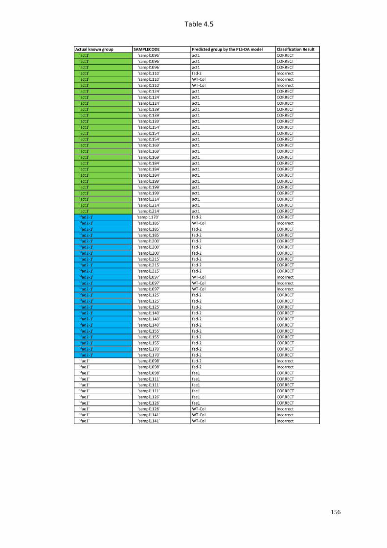
156
Table 4.5
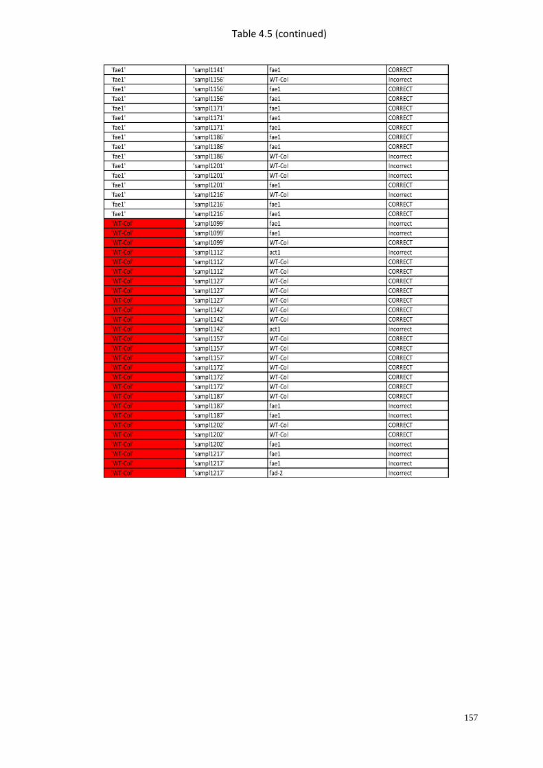
157
Table 4.5 (continued)
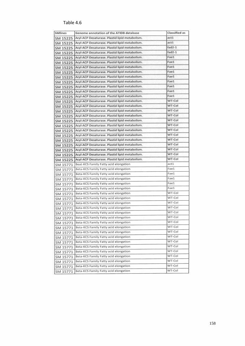
158
Table 4.6
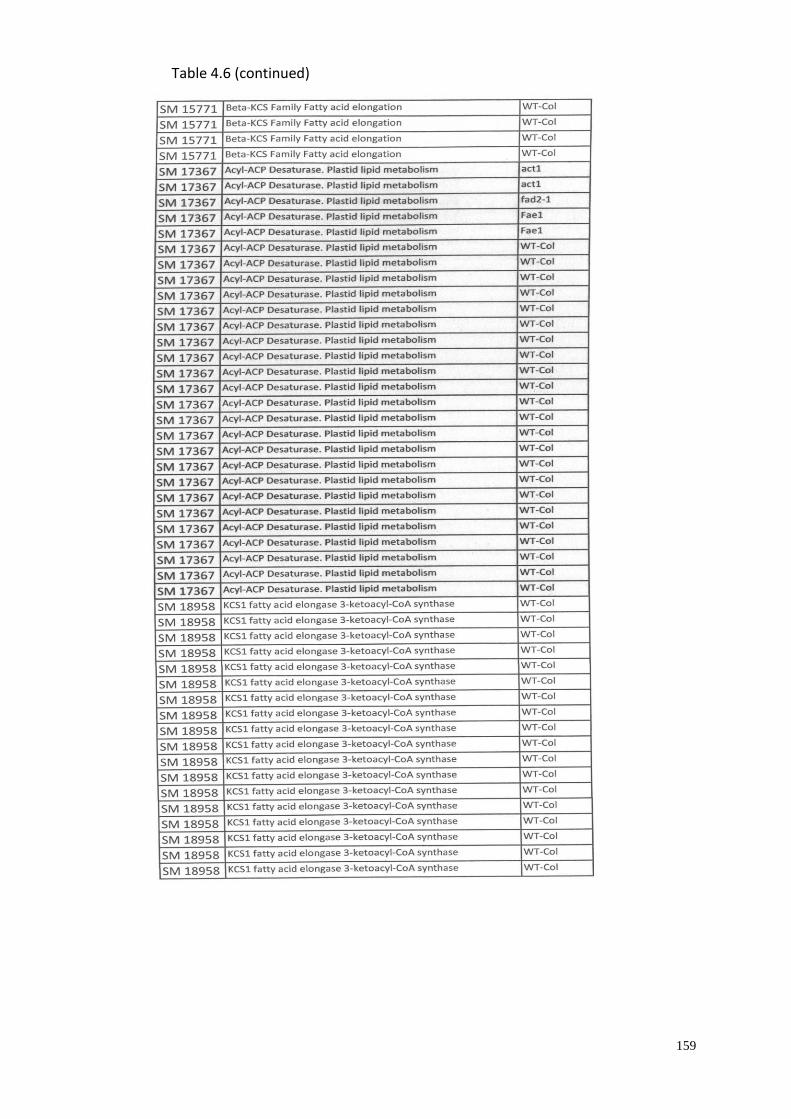
159
Table 4.6 (continued)
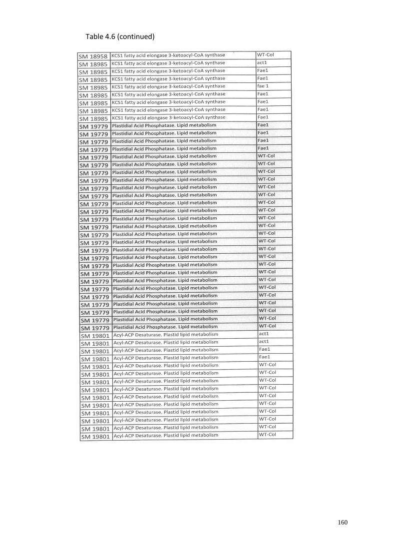
160
Table 4.6 (continued)
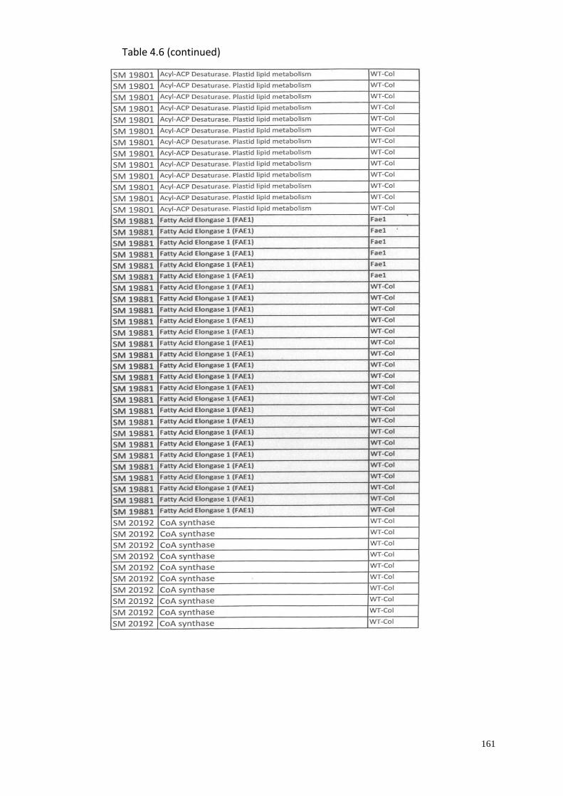
161
Table 4.6 (continued)
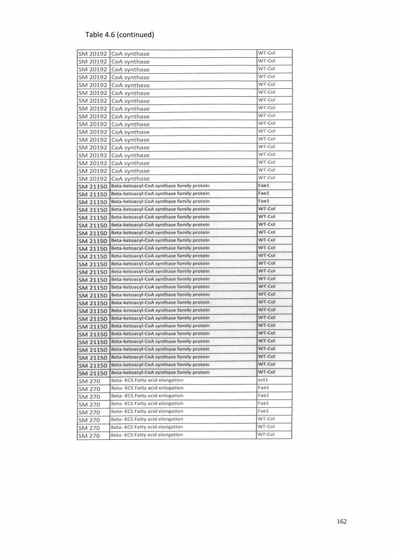
162
Table 4.6 (continued)
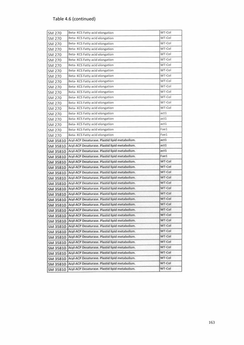
163
Table 4.6 (continued)

164
APPENDIX A3:
SUPPLEMENTARY MATERIAL FOR CHAPTER 5
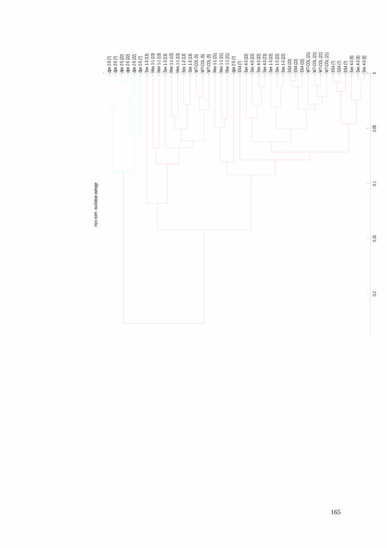
165
00.
050.
10.
150.
2
Sex
4-3
(5)
Sex
4-3
(5)
Sex
4-3
(5)
SS
4 (7
)
SS
4 (7
)
SS
4 (7
)
WT-
CO
L (2
1)
WT-
CO
L (2
1)
WT-
CO
L (2
1)
WT-
CO
L (2
1)
SS
4 (2
2)
SS
4 (2
2)
SS
4 (2
2)
Sex
1-3
(22)
Sex
1-3
(22)
Sex
1-3
(22)
Sex
4-3
(21)
Sex
4-3
(22)
Sex
4-3
(22)
Sex
4-3
(22)
SS
4 (7
)
dpe
2-5
(7)
Mex
1-1
(21)
Mex
1-1
(21)
Mex
1-1
(21)
WT-
CO
L (5
)
WT-
CO
L (5
)
WT-
CO
L (5
)
Sex
1-3
(13)
Sex
1-3
(13)
Mex
1-1
(13)
Mex
1-1
(13)
Sex
1-3
(13)
Mex
1-1
(13)
Mex
1-1
(13)
Sex
1-3
(13)
dpe
2-5
(7)
dpe
2-5
(22)
dpe
2-5
(22)
dpe
2-5
(22)
dpe
2-5
(7)
dpe
2-5
(7)
myx
norm
eucl
idea
n aver
age