Embed Size (px)
Citation preview
Pore-Scale Network Modeling of Microporosity in Low-
Resistivity Pay Zones of Carbonates
By
© 2019
Nijat Hakimov
B.Sc., Azerbaijan State Oil Academy, 2013
Submitted to the graduate degree program in Chemical and Petroleum Engineering
and the Graduate Faculty of the University of Kansas in partial fulfillment of the
requirements
for the degree of Master of Science.
Chair: Dr. Amirmasoud Kalantari-Dahaghi
Dr. Shahin Negahban
Dr. Arsalan Zolfaghari
Date Defended: 3rd of June, 2019
i
The thesis committee for Nijat Hakimov certifies that this is
the approved version of the following thesis:
Pore-Scale Network Modeling of Microporosity in Low-
Resistivity Pay Zones of Carbonates
Chair: Dr. Amirmasoud Kalantari-Dahaghi
Date Approved: 3rd of June, 2019
ii
Abstract
Carbonates present an important research area as classical empirical methods primarily
developed for sandstone characterizations give erroneous results when being applied to
carbonates. Specifically, the question of applicability of the Archie equation for these
rocks is of great interest in the industry since it is directly related to reserves estimation.
Archie equation often calculates high water saturation for intervals dominated by
carbonates which would yield zero or little water-cut when being put on production. This
phenomenon is known as “Low Resistivity Pay” (LRP). The problem arises from the
inherent multi-scale heterogeneity of these rock types where different scales of pore
populations constitute the pore space. As a result, the traditional techniques employed in
digital rock physics has to be modified for accurate descriptions of the pore space in
carbonates. Here in this work, we develop a state-of-the-art pore-scale network model
(PSNM) that populates pore space for the microporous zones of carbonates and
consequently, simulates displacement sequences during drainage and imbibition. To
generate representative pore networks, the digital 3D images of the pore space should
be larger than the representative elementary volume (REV) of the sample where all the
effective pore space (i.e., contributing to the flow) are fully resolved. Existence of mixed-
wet states in carbonates reduces the minimum pore sizes that contribute to the flow of
the wetting phase. At the same time, inherent heterogeneity of carbonates increases their
REV. This means that high-resolution images of large sample volumes have to be
collected and processed. This, however, is not possible due to the physical and
computational power limitations of the current imaging tools and computers. Therefore, it
is often the case that the 3D image of a REV does not have high enough resolution, thus,
iii
overlooking a large number of micropores, which usually account for a significant portion
of the pore space in carbonates.
In this work, we develop a PSNM to investigate microporosity impact on the electrical and
transport properties of 2D (lattice-based) and 3D pore networks. We have addressed the
resolution problem by generating stochastic pore networks spatially located within the
domains of unresolved zones (i.e., microporosity). The model stochastically reconstructs
the pore space at higher resolutions based on the given input parameters of local porosity
and pore size distribution for the microporous zones. We use two carbonate samples:
one outcrop of Estaillades limestone and one reservoir limestone. The latter is taken from
the Mississippian formation of the Osagean age in the STACK play in Oklahoma. For this
interval, traditional techniques suggest high water saturation, however, core analysis
reveals a significant oil saturation throughout the zone.
The results indicate a strong effect of the pore size distribution on the electrical and
transport properties of these carbonate samples. The model allows to simulate and
explain non-Archie behavior of the Resistivity Index curve. It also allows investigating the
extent to which microporosity can have an impact on the petrophysical properties of
carbonates by identifying key parameters with the biggest impact on the simulated
properties.

iv
Acknowledgments
First of all, I would like to express my deepest appreciation to my graduate advisor Dr.
Amirmasoud Kalantari-Dahaghi for giving me this opportunity to join his research team
back in Fall 2017 and for his support and help during my research project. Also, I would
like to extend my deepest gratitude to one of the most hard-working people I have ever
met — Dr. Arsalan Zolfaghari — for helping me numerous times to overcome very tough
obstacles during my research and for being to me as a brother and as a friend at the times
when I needed support. I appreciate the constant help that he has offered me even
outside academia. Besides, I am very grateful to Prof. Shahin Negahban for his helpful
comments on my project and I sincerely appreciate the time he took to hold frequent
meetings with me to share his expertise in the field of my research.
Also, I am very thankful to Gary Gunter from Schlumberger and Geoff Vice from Fairway
Resources for their useful feedback on my research project. I also would like to thank
Prof. Paul Willhite for supervising me during my first semester at KU when I was working
as a TA for his class.
Also, I would like to extend my sincere thanks to Martha Kehr at the CPE department for
her help and support during all these years at KU. I am also grateful to all of my co-
workers and friends and all the kind people that I met here and which supported me and
helped me during this long journey.
And last, but not least, as for everything in life, I’m always thankful to my parents and to
my brother for their endless support, love, and belief in me.
v
Table of Contents
Chapter 1. Introduction and problem statement ..............................................................vi
Chapter 2. Literature Review ........................................................................................... 9
Chapter 3. Methods ....................................................................................................... 14
3.1. Quasi-static Pore-Network Modelling Simulations of Primary Drainage and
Imbibition ................................................................................................................... 14
3.2. 2D pore networks generation. ............................................................................. 17
3.3. 3D pore-networks generation ............................................................................. 22
3.3.1. Samples used in this work ............................................................................ 22
3.3.2. 3D Image acquisition and segmentation ...................................................... 22
3.3.3. Stochastic pore-network generation ............................................................. 24
3.4. Calculation of electrical properties ...................................................................... 31
3.5. Tortuosity calculations ........................................................................................ 34
Chapter 4. Results......................................................................................................... 38
4.1. 2D pore-networks with introduced microporosity. Sensitivity of resistivity index
and tortuosity to increasing microporosity. ................................................................. 38
4.2. 3D pore networks. Effect of wide pore size distribution on the electrical
properties. .................................................................................................................. 45
4.2.1. Archie’s calculated water saturation ............................................................. 46
4.2.2. Comparison to Berea sandstone .................................................................. 48
4.3. 3D pore-networks. Impact of microporosity related parameters on electrical and
transport properties of the rock sample. .................................................................... 51
4.3.1. Capillary pressure results ............................................................................. 57
4.3.2. Relative permeability results ........................................................................ 59
4.3.3. Resistivity Index results ................................................................................ 62
4.3.4. Impact on reserves estimation. .................................................................... 67
Chapter 5. Discussion & conclusion .............................................................................. 68
References .................................................................................................................... 70
Appendices ................................................................................................................... 75
vi
List of Figures
Figure 3.1. Example matrix generated for a 2D pore-network numbering representation.
...................................................................................................................................... 18
Figure 3.2. Illustration of the equilateral triangular pore and two throats with the same
cross-sectional shape connected to it. L is used to denote the length of the pore. ....... 19
Figure 3.3. Illustration of a 2D lattice pore network where red dots represent pore centers
...................................................................................................................................... 19
Figure 3.4. Two identical macro-pore networks: a small example of base pore network
(top) and a modified pore network with microporosity (bottom) ..................................... 21
Figure 3.5. The raw 3D micro-CT scan image of the sample with the resolution of 3.1 µm
(A), phases extracted the image segmentation overlaid on the original micro-CT scan
image after (B): blue color represents microporosity, red — macropore space. ............ 23
Figure 3.6. Resolved (macro) pore space (A) and its corresponding pore network where
pore and throat radii demonstrate the largest inscribed radii (B). .................................. 24
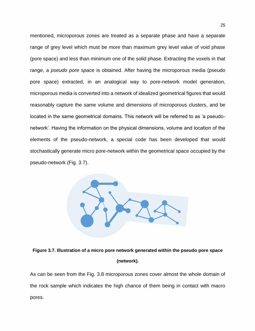
Figure 3.7. Illustration of a micropore network generated within the pseudo pore space
(network). ...................................................................................................................... 25
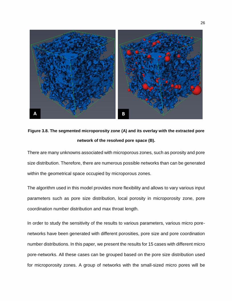
Figure 3.8. The segmented microporosity zone (A) and its overlay with the extracted pore
network of the resolved pore space (B). ........................................................................ 26
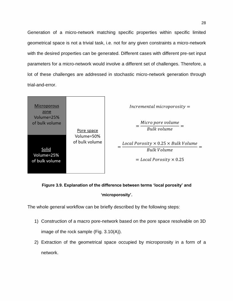
Figure 3.9. Explanation of the difference between terms ‘local porosity’ and
‘microporosity’. .............................................................................................................. 28
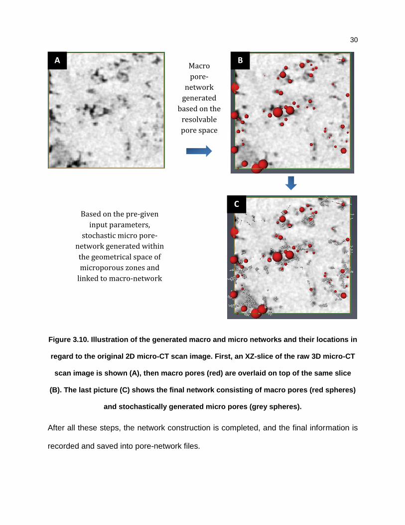
Figure 3.10. Illustration of the generated macro and micro networks and their locations in
regard to the original 2D micro-CT scan image. First, an XZ-slice of the raw 3D micro-CT
scan image is shown (A), then macro pores (red) are overlaid on top of the same slice
(B). The last picture (C) shows the final network consisting of macro pores (red spheres)
and stochastically generated micro pores (grey spheres). ............................................ 30
Figure 3.11. Kirchhoff's current law under a steady-state condition for a pore with the
coordination number of 5. .............................................................................................. 33
Figure 3.12. Geometrical tortuosity is calculated as the ratio of the shortest pathway
length to the straight-line (end-to-end) length. ............................................................... 35
vii
Figure 3.13. Illustration of the difference between geometrical and hydraulic tortuosity.
For the same porous media, the left picture depicts the shortest pathway length used for
geometrical tortuosity calculation, the right picture shows converging-diverging
streamlines that are considered for hydraulic tortuosity calculation. ............................. 36
Figure 3.14. An example of one of the pathway lengths and end-to-end length for a pore
network .......................................................................................................................... 36
Figure 4.1. Five different groups of pore networks with microporosity used in this study.
...................................................................................................................................... 38
Figure 4.2. Electrical resistance versus water saturation during drainage and imbibition
processes for the first group of generated networks where random horizontal macro-
throats are replaced with micro-networks. ..................................................................... 41
Figure 4.3. Electrical resistance versus water saturation during drainage and imbibition
processes for the second group of generated networks where random vertical macro-
throats are replaced with micro-networks. ..................................................................... 42
Figure 4.4. Electrical resistance versus water saturation during drainage and imbibition
processes for the third group of generated networks where random vertical macro-throats
are removed and random horizontal macro-throats are replaced with micro-networks. 43
Figure 4.5. Electrical resistance versus water saturation during drainage and imbibition
processes for the fourth group of generated networks where random horizontal macro-
throats are removed and random vertical macro-throats are replaced with micro-networks.
...................................................................................................................................... 44
Figure 4.6. Electrical resistance versus water saturation during drainage and imbibition
processes for the fifth group of generated networks where both random vertical and
horizontal macro-throats are replaced with micro-networks. ......................................... 45
Figure 4.7. The pore network of Estaillades limestone generated from 3D CT-scan image
of a dry sample. Note: some of the pores or throats are not clearly visible due to their
small radii. ..................................................................................................................... 46
Figure 4.8. The comparison of Archie’s calculated water saturation and actual water
saturation from the PNM of Estaillades-1 sub-volume during primary drainage. ........... 48
viii
Figure 4.9. Pore networks of the Berea sandstone on the left and Estaillades limestone
on the right. Note: throats are hidden to make pores more visible. Sphere sizes represent
each pore volume. ......................................................................................................... 49
Figure 4.10. Pore Network of the Estaillades-2 sub-volume where the blue arrow shows
the injection direction. Note: throats are hidden to make pores more visible. ................ 50
Figure 4.11. The comparison of pore size distributions for the Berea sandstone and
Estaillades limestone. .................................................................................................... 50
Figure 4.12. The electrical resistivity of the Berea sandstone and Estaillades limestone
during primary drainage. ............................................................................................... 51
Figure 4.13. Comparison of the pore coordination number distributions for stochastically
generated networks: S-10 (with small-sized micro pores), M-10 (with medium-sized micro
pores) and L-10 (with large-sized micro pores). Note: bars for coordination numbers
higher than 11 are not shown because of very low frequency for all three networks. ... 54
Figure 4.14. Bar chart with the comparison of the number of pores and throats, isolated
and total porosity for all the generated networks. .......................................................... 55
Figure 4.15. Bar chart with the comparison of the absolute permeability, incremental
microporosity, isolated and total porosity for all the generated networks. Note: absolute
permeability for L-10 is not visible on the graph due to very low value compared to
permeability axis scale. ................................................................................................. 56
Figure 4.16. Capillary pressure curves during primary drainage generated for the pore-
networks with small micro pores in microporosity zones. .............................................. 57
Figure 4.17. Capillary pressure curves during primary drainage generated for the all pore-
networks. Red curves represent S-networks (small-sized micro pores), blue — M-
networks (medium-sized micro pores) and green — L-networks (large-sized micro pores).
Transparent areas are shown in order to group the results in separate clusters. .......... 58
Figure 4.18. Relative permeability curves during primary drainage generated for the pore-
networks with the small-sized micro pores in microporosity zones. .............................. 60
Figure 4.19. Relative permeability curves during primary drainage generated for the all
pore-networks. Red curves represent S-networks (small-sized micro pores), blue — M-
networks (medium-sized micro pores) and green — L-networks (large-sized micro pores).
Relative permeability axis is shown in log-scale. For the purpose of more clear
ix
visualization, oil relative permeability curve is not connected all the way till zero value, i.e.
only non-zero values of oil relative permeability are plotted and connected. ................. 61
Figure 4.20. Approximate type curves determined based on the results for relative
permeability during primary drainage for three groups of pore-networks. Red curve
corresponds to the group of pore-networks with the small-sized pores in microporosity
zone, green — to the group with the medium-sized micropores and blue — to the group
with the large-sized micropores. Relative permeability axis is shown in log-scale. ....... 62
Figure 4.21. Resistivity Index curves during primary drainage generated for the pore-
networks with small micropores in microporosity zones. Both axes are shown in log-scale.
...................................................................................................................................... 63
Figure 4.22. Pore Size Distribution comparison for three generated pore-networks (S-10,
M-10, L-10) with the same local porosity (10%) but with the different micro pore sizes. 64
Figure 4.23. Visual comparison of three generated pore-networks (S-10, M-10, L-10) with
the same local porosity (10%) but with the different micro pore sizes. .......................... 65
Figure 4.24. Resistivity Index curves during primary drainage generated for all pore-
networks. Red curves represent S-networks (small-sized micro pores), blue — M-
networks (medium-sized micro pores) and green — L-networks (large-sized micro pores).
Transparent grey areas are shown in order to group the results in one cluster. ............ 66
Figure 4.25. The plot shows by how much (%) the reserves estimated using Archie
equation would differ from the actual value. .................................................................. 67
Figure A-1. Capillary pressure curves during primary drainage generated for the pore-
networks with the medium-sized micro pores in microporosity zones. .......................... 75
Figure A-2. Capillary pressure curves during primary drainage generated for the pore-
networks with the large-sized micro pores in microporosity zones. ............................... 76
Figure A-3. Relative permeability curves during primary drainage generated for the pore-
networks with the medium-sized micro pores in microporosity zones. .......................... 77
Figure A-4. Relative permeability curves during primary drainage generated for the pore-
networks with the large-sized micro pores in microporosity zones. ............................... 78

x
Figure A-5. Resistivity Index curves during primary drainage generated for the pore-
networks with the medium-sized micro pores in microporosity zones. Both axes are
shown in log-scale. ........................................................................................................ 79
Figure A-6. Resistivity Index curves during primary drainage generated for the pore-
networks with the large-sized micro pores in microporosity zones. Both axes are shown
in log-scale. ................................................................................................................... 80
Figure A-7. Five different groups of 2D pore networks with their included microporosity
regions. Base pore networks are shown on the left. Same pore networks with the inserted
micro-networks in red are shown on the right. ............................................................... 81
Figure A-8. The percentages of microporosity regions and the electrical and flow
tortuosities in all pore networks generated in this work. ................................................ 82
Figure A-9. Pore Network of the Estaillades-2 sub-volume where both pores and throats
are shown. ..................................................................................................................... 83
List of Tables
Table 1.1. Micro-CT scanner resolutions (Xiong et al., 2016). ........................................ 3
Table 1.2. Summary of the existing pore-scale flow simulation models. ......................... 3
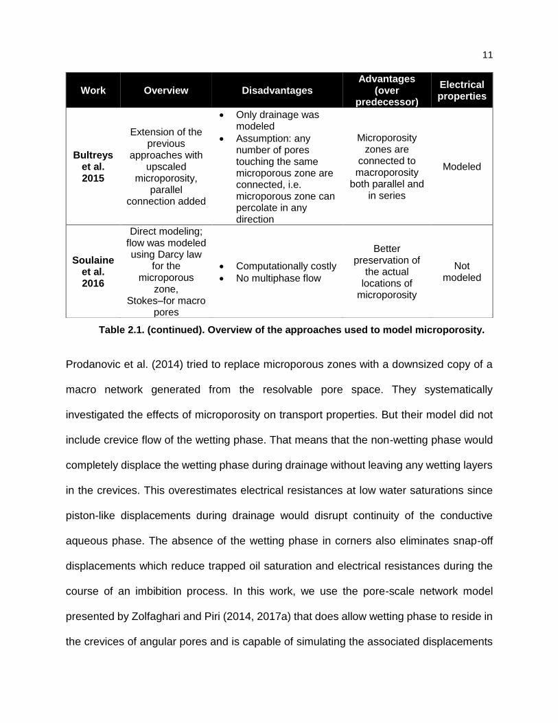
Table 2.1. Overview of the approaches used to model microporosity. .......................... 10
Table 3.1. All the generated pore-networks named based on the pore size and porosity.
...................................................................................................................................... 27
Table 3.2. The analogy between transport and electrical properties ............................. 32
Table 4.1. Summary of the properties for the all generated pore networks. .................. 52

1
Chapter 1. Introduction and problem statement
The first chapter introduces the main tools and concepts that have been used in this work.
Particularly, first of all, we discuss the importance of the research on carbonates and the
challenges associated with them. We specifically consider two major problems that the
researchers encounter while dealing with carbonates in two different areas. Secondly, we
discuss the common cause of these problems — microporosity — and review the general
pore space characterization methods commonly used in Digital Rock Physics to address
these problems. Finally, we specifically focus on the technique used in this work called
Pore-Network Modelling (PNM) and present the ideas and the assumptions it is based
on.
Experts estimate that carbonate reservoirs hold more than 60% of the world’s oil reserves
and 40% of the world’s gas reserves (Ahmed 2010, Al-Marzouqi et al. 2010, Sheng 2013).
Especially, for the Middle East region, the statistics get even more drastic with carbonate
formations accounting for 70% of oil and 90% of gas reserves (Gundogar et al. 2016).
These numbers spotlight the strategic importance of carbonate reservoirs in the context
of future energy supply. Therefore, it is of great significance to accurately characterize
carbonates, especially, considering the extremely complex nature of these formations.
Generally, porous media characterization has always been a major area of research in
different fields, such as petroleum engineering, hydrology, and environmental and
biological sciences. Various studies have shown the linkage between small scale events
at the pore level and their corresponding large scale effect at the core level. Over the past
few years, a lot of attention has been attracted to develop models for the simulation of
2
different pore-scale events. With the recent development of supercomputers and imaging
technologies, our understanding of different pore-level physics has been improved.
However, there are still unaddressed challenges, particularly, with respect to some of the
commonly used hypotheses and scale-up issues.
From the modeling point of view, the first important step is to obtain a representative pore
space structure for the medium of interest. This can be done by various imaging
techniques, using different modalities (Xiong et al., 2016), or other methods such as,
Mercury Intrusion Porosimetry (MIP) (Leon y Leon, 1998) and Gas Adsorption (Thommes
et al., 2006). Non-imaging techniques can provide little details about the complex topology
of the pore space. They are primarily limited to extraction of pore size distribution with the
assumption that injected fluid has access to all and every pore and throat. Imaging
techniques, on the other hand, can be used to characterize topological properties of a
sample for each individual pore and throat as long as resolution allows. These techniques
include X-ray computed micro-tomography (micro-CT), scanning electron microscopy
(SEM) with Focused Ion Beams (FIB). Maximum resolution of SEM alone can vary in the
range of 1-20 nm, while FIB can go lower down to less than 1 nm. Combination of these
two techniques allows achieving voxel dimensions of tens of nanometers (Xiong et al.,
2016). However, FIB/SEM is destructive imaging method, while micro-CT imaging
techniques are non-destructive and non-invasive, and they are the most commonly used
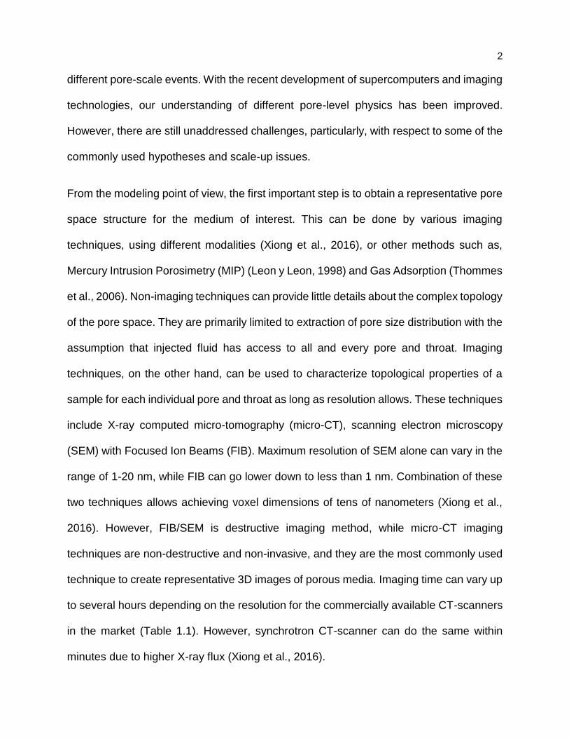
technique to create representative 3D images of porous media. Imaging time can vary up
to several hours depending on the resolution for the commercially available CT-scanners
in the market (Table 1.1). However, synchrotron CT-scanner can do the same within
minutes due to higher X-ray flux (Xiong et al., 2016).
3
CT scanner Spatial resolution
Medical 200-500 µm
Industrial 2-100 µm
Synchrotron 1-50 µm
Table 1.1. Micro-CT scanner resolutions (Xiong et al., 2016).
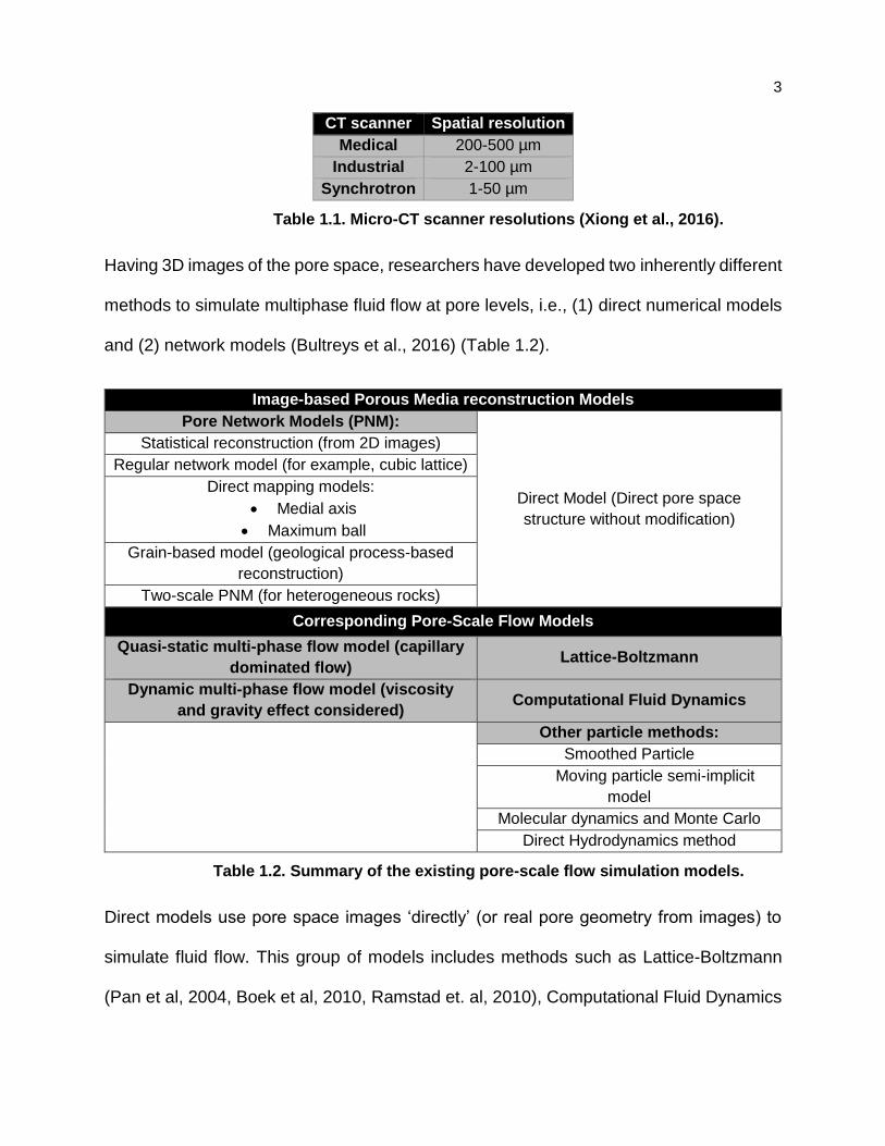
Having 3D images of the pore space, researchers have developed two inherently different
methods to simulate multiphase fluid flow at pore levels, i.e., (1) direct numerical models
and (2) network models (Bultreys et al., 2016) (Table 1.2).
Image-based Porous Media reconstruction Models
Pore Network Models (PNM):
Statistical reconstruction (from 2D images)
Regular network model (for example, cubic lattice)
Direct mapping models:
• Medial axis
• Maximum ball
Direct Model (Direct pore space
structure without modification)
Grain-based model (geological process-based
reconstruction)
Two-scale PNM (for heterogeneous rocks)
Corresponding Pore-Scale Flow Models
Quasi-static multi-phase flow model (capillary
dominated flow) Lattice-Boltzmann
Dynamic multi-phase flow model (viscosity
and gravity effect considered) Computational Fluid Dynamics
Other particle methods:
Smoothed Particle
Moving particle semi-implicit
model
Molecular dynamics and Monte Carlo
Direct Hydrodynamics method
Table 1.2. Summary of the existing pore-scale flow simulation models.
Direct models use pore space images ‘directly’ (or real pore geometry from images) to
simulate fluid flow. This group of models includes methods such as Lattice-Boltzmann
(Pan et al, 2004, Boek et al, 2010, Ramstad et. al, 2010), Computational Fluid Dynamics
4
(CFD) (Raeini et al., 2015, Icardi et al., 2014), and Inscribed Sphere Movement
(Mohammadmoradi et al., 2017). These models are computationally expensive and
instable (Meakin et al., 2009). They are mostly developed for 2D images, single phase
flow, and has not reached to the level to reliably predict relative permeability and capillary
pressures even in more homogenous systems. It is interesting to note that not many
researchers have tried to simulate multiphase flow using direct methods. Raeini et al.
(2015) tried to study capillary trapping impact by solving full Navier-Stokes equations for
two-phase flow on micro-CT images of Berea sandstone and LV60 sandpack. They
compared the results to the experiment and to quasi-static Pore-Network Modeling (PNM)
simulation. They showed a better match for the direct simulation results with that of the
experiments. Their PNM simulations had significant deviation from the experimental
results. Direct simulation results matched the experiment, while PNM simulation predicted
higher residual non-wetting phase saturation for water injection in the direction reverse to
primary drainage, especially for LV60 sandpack. However, it is worth to mention that
viscosity and density for both fluids were to set to that of water at room temperature.
LBM has been successfully used for single flow simulations, however, multiphase flow
simulation involves a lot of challenges, due to numerical instability it becomes problematic
to implement it for multiphase flow of fluids with large density and viscosity ratios (for
example, water-gas systems) (Meakin et al., 2009, Chin et. al, 2002).
Not many researchers have tried to simulate multiphase flow directly on pore-scale
images. The early works were done on two-dimensional models without comparison to
experimental data (Pan et. al, 2004). Boek et al. (2010) conducted Latice-Boltzmann
simulations for single-phase flow on 2D micro-model of Berea and for two-phase flow on
5
3D model of Bentheimer. However, the generated relative permeability data was not
compared to the experimental one. Ramstad et al. (2012) simulated steady-state and
unsteady-state experiments of two-phase flow using Lattice-Boltzmann on micro-CT
images of Bentheimer and Berea samples. The results were in a good agreement with
the reported experimental data, except non-wetting-phase relative permeability for
drainage, which was calculated from production and pressure data; authors explained
that with viscous instabilities (viscous fingering) which contradict Darcy’s law assumptions
for two-phase flow. Raeini et al. (2015) tried to study capillary trapping effect by solving
full Navier-Stokes equations for two-phase flow on micro-CT images of Berea sandstone
and LV60 sandpack, and compared the results with the experiment and quasi-static PNM
simulation. One of the common problems encountered during Lattice-Boltzmann-based
simulations of two-phase flow is wetting film thickness being smaller than voxel size,
which can lead to erroneous results. (Raeini et al., 2015, Ahrenholz et al., 2008, Vogel et
al., 2005)
The other disadvantage of Direct Simulation methods is much smaller scale of simulation
compared to PNM, while PNM simulations can go up to close to core scale (Blunt et al.,
2013).
In Pore-Network Models (PNM) — the second group of models — the pore space is
characterized by a network of pores connected by throats with idealized and constant
cross-sectional geometries. Researchers have used different cross-sectional shapes
including circle, triangle, square, rectangle, star, and ellipse. Such simple geometries are
particularly chosen to calculate the corresponding threshold capillary pressures of
displacements using more computationally efficient analytical approaches. This is

6
because ‘threshold capillary pressures’ and ‘phase connectivities’ are primarily used to
determine displacement sequences at pore levels. Most pore network models are
developed under quasi-static conditions where capillary forces are solely responsible for
fluid displacements at pore levels (Blunt et al. 2002, 2013; Piri and Blunt 2005a, Zolfaghari
2017a, 2017b). This assumption is reasonably valid when we determine the key forces
controlling the physics of flow through porous media. At the pore scale level, due to very
small fluid velocities, viscous forces become negligible compared to capillary forces
(Satter and Iqbal 2015). Despite that fact, researchers have also been able to expand the
capability of Pore-Network Models to incorporate viscous and gravitational forces
(Joekar-Niasar et al. 2010, Sheng and Thompson 2013, Aghaei and Piri 2015). Although
there is a still a lot of discussion around the experimental validation of the results obtained
from PNM simulation (Oren 1997, Piri and Blunt 2005b, Piri and Karpyn 2007, Aghaei
and Piri 2015, Zolfaghari and Piri 2016, Yang 2017), the latest model with the cooperative
pore-body filling presented by Ruspini et al. 2017 showed the capability of the PNM to
predict the experimental measurements. In addition, the research has been done by Miao
et al. (2017) to create a pore network without pore shape simplifications. In that model
single-phase hydraulic conductance of the actual pore element (without idealization of
geometry) is predicted by the Neural Network based on three parameters describing a
pore element: circularity, elongation and convexity. Using CFD, Navier-Stokes equation
was solved and hydraulic conductance data was generated for 3292 pore elements and
was used to train the Neural Network. 90% of hydraulic conductance predictions lied
within an accuracy of ±20%. This might be the first step in creating a model which would
combine both accuracy and efficiency at the same time.
7
Considering the advantages that PNMs can offer in comparison to direct methods, one
can find them more suitable for the purpose of studying the electrical and transport
properties of carbonates.
However, characterization of the carbonate rocks still remains challenging due to the
existence of complex multiscale pore structures and their connectivity. This causes
considerable heterogeneity at different scales presenting a tough challenge for engineers
and geologists in determining the performance of the carbonate reservoirs. One of these
challenges comes from the fact that most of the traditionally used models for studying
transport and electrical properties are developed for siliciclastic rocks which may give
erroneous results when being applied to carbonates (Talabani et al. 2000; Doveton 2001;
Bauer et al. 2011; Prodanovic et al. 2014). Depositional history of carbonate rocks makes
them completely different from siliciclastic rocks (Akbar et al. 2000; Ahr 2011). The latter
ones are composed of pieces (usually, well-sorted) of the other rocks that were eroded
by weathering processes, while most of the carbonates are made up from the fragments
of calcareous organisms (Akbar et al. 2000). Therefore, one can expect more
homogenous pore space in clastic rocks than in carbonates. Later diagenetic alterations
drastically increase heterogeneity which is likely to occur in carbonates due to their brittle
nature and vulnerability of their minerals to dissolution (Akbar et al. 2000; Bear et al.
2012). This causes the pore space in carbonates to undergo various morphological
changes, ultimately, becoming very heterogeneous. Thus, carbonates contain not only
interparticle but also intraparticle porosity. The latter is usually referred to as
microporosity. The recent works have shown that microporosity can account for a very
significant portion of the pore space in carbonates which emphasizes the importance of
8
its effect on the electrical and transport properties of these rocks (Norbisrath et al. 2015;
Gundogar 2016).
Traditional techniques used in Digital Rock Physics also fail to provide an accurate pore
space description for carbonates because of their extreme heterogeneity within a small
volume. The challenge arises due to the selection of an appropriate scale that represents
their wide pore size distributions. Regardless of the resolution, pore sizes in the
microporosity zones are often below the resolution of the tool being used (Blunt et al.
2013; Bultreys et al. 2015). On one hand, a 3D image of porous media should cover a
larger volume than its Representative Elementary Volume (REV). On the other hand, it
should have high enough resolution to capture smaller pores. That causes the problem
of scale where sub-resolution microporosity regions exist in pore-scale images regardless
of the imaging technique being employed (e.g., micro-CT scanning). Since pore space
topology cannot be captured in these unresolved regions, they are often ignored in the
pore-scale models. Assuming microporous zone as a void space or as a nonporous solid
will result in incorrect predictions of flow and electrical properties such as absolute and
relative permeabilities, capillary pressure, and formation factor (Bultreys et al. 2015;
Norbisrath et al. 2015; Soulaine et al. 2016). It should be noted that for monomineralic
rocks, although individual micro-pores cannot be imaged, the regions with microporosity
can be identified based on their gray level range on gray-scale images of the pore space
(Bultreys et al. 2015).
9
Chapter 2. Literature Review
Over the last few years, there have been several attempts to develop modeling
techniques for studying microporosity and its impact on the flow and electrical properties.
Particularly, some researchers have tried to incorporate microporosity into the PNMs
(Prodanovic et al. 2014, Bultreys et al. 2015). To incorporate microporosity regions, one
should obtain a 3D image of an REV (or a larger volume) that has high enough resolution
to capture micro pores. This would generate a huge amount of voxels which is beyond
the processing capabilities of the modern computers (Jiang et al. 2013). Several authors
have tried to circumvent capturing the actual pore space of microporosity by modifying
PNMs to accommodate different scales. Table 2.1 provides a brief overview of the
approaches that have been used to model microporosity.
Bekri et al. (2005) introduced one of the first dual PNMs with a lattice network of macro
pores and parallel microporous matrixes. To model the flow, upscaled known properties
were assigned to the matrix including porosity, permeability, capillary pressure, and
relative permeability curves. Bauer et al. (2011, 2012) followed the same approach by
modeling microporous zones as the blocks of continuous porous media. In their work,
each block connects two macro pores parallel to the linking macro-throat. Jiang et al.
(2013) built multi-scale pore networks with individual pores for microporosity zones. In
their model, representative networks were first generated from images at distinct length
scales. A stochastic method was then used to generate a larger network based on the
statistical information gathered from networks of different scales.

10
Table 2.1. Overview of the approaches used to model microporosity.
Work Overview Disadvantages Advantages
(over predecessor) Electrical properties
Bekri et al. 2005
Vugs/fractures are modelled as a
lattice network of macro pores with the microporous
matrix, the microporous zone
is treated as continuous porous
media
• Microporosity acts only in parallel
• Only drainage was modeled
• Does not contain pore networks for microporous zones
As all PNMs, has less computational time in comparison with direct models /
Less complex
Modeled
Bauer et al. 2011, 2012
Microporous zones are
represented as blocks of
continuous porous media connecting
2 macro pores that are already
connected through a macro
throat
• Microporous zones are connected to macro pores only in parallel
• Does not contain pore networks for microporous zones, microporosity is modeled as continuous porous media
Crevice flow was modeled
Modeled
Jiang et al. 2013
Actual pore network for a
random microporosity
zone is generated and used to
generate a larger pore network that
would fit the macro network
domain
Impractical computational cost
and time
• Better representation of microporosity/ individual micro pores
• Better representation of cross-scale connectivity
Not Modeled
Prodanovic et al. 2014, Mehmani
and Prodanovic
2014
A copy of macro network reduced
in size and mapped on microporous
zones
Crevice flow of the wetting phase not
modeled
A model with individual micro pores, without
upscaling
Not Modeled
11
Table 2.1. (continued). Overview of the approaches used to model microporosity.
Prodanovic et al. (2014) tried to replace microporous zones with a downsized copy of a
macro network generated from the resolvable pore space. They systematically
investigated the effects of microporosity on transport properties. But their model did not
include crevice flow of the wetting phase. That means that the non-wetting phase would
completely displace the wetting phase during drainage without leaving any wetting layers
in the crevices. This overestimates electrical resistances at low water saturations since
piston-like displacements during drainage would disrupt continuity of the conductive
aqueous phase. The absence of the wetting phase in corners also eliminates snap-off
displacements which reduce trapped oil saturation and electrical resistances during the
course of an imbibition process. In this work, we use the pore-scale network model
presented by Zolfaghari and Piri (2014, 2017a) that does allow wetting phase to reside in
the crevices of angular pores and is capable of simulating the associated displacements
Work Overview Disadvantages Advantages
(over predecessor)
Electrical properties
Bultreys et al. 2015
Extension of the previous
approaches with upscaled
microporosity, parallel
connection added
• Only drainage was modeled
• Assumption: any number of pores touching the same microporous zone are connected, i.e. microporous zone can percolate in any direction
Microporosity zones are
connected to macroporosity
both parallel and in series
Modeled
Soulaine et al. 2016
Direct modeling; flow was modeled using Darcy law
for the microporous
zone, Stokes–for macro
pores
• Computationally costly
• No multiphase flow
Better preservation of
the actual locations of
microporosity
Not modeled
12
such as snap-off. Bauer et al. (2011) pointed out the importance of wetting layers for
accurate modeling of electrical properties. They showed that resistivity index is hugely
overestimated for Fontainebleau sandstone when the wetting film is not modeled. Besides
sandstone, they investigated the electrical properties of carbonates with a major limitation
in their model: microporous zones were only connected in parallel to the macro pore
networks. Bultreys et al. (2015) have also used a similar approach of treating
microporosity as a continuous porous media and assigning upscaled properties.
However, they allowed both parallel and in-series connections for the linking of
microporosity zones to macro pore networks. In these works, the upscaled properties are
usually estimated based on the gray level of microporous zones, which is valid only for
monomineralic rocks (Bultreys et al. 2015).
Besides PNMs, direct modeling techniques have been also used for fluid flow modeling
in the pore space of various rock samples (Blunt et al. 2013; Bultreys et al. 2016). As was
mentioned, these techniques use an actual geometry of the pore space (i.e., without
simplifications of the pore networks) to solve governing equations of flow. Microporosity
still remains a challenge due to being unresolved. Recently, Soulaine et al. (2016) used
a direct model consisting of Stokes equation for macro pores and Darcy equation for
microporosity regions. Authors successfully calculated absolute permeability of Berea
sandstone from images with 2% subresolution porosity. They reported 60%
overestimations of the permeability for the cases where microporous zones are
mistakenly replaced with the void space. As mentioned, microporosity greatly impacts
transport and electrical properties of samples with wide pore size distributions (Bekri et
al. 2005; Bauer et al. 2011, 2012). The specific problem associated with the electrical
13
properties has been also referred to “Low Resistivity Pay” (LRP) phenomenon in the oil
and gas industry (Boyd et al. 1995, Coates et al. 1999). Formation resistivity is often
measured during well logging operations which is then correlated to the water saturation.
This water could be however mobile, partially mobile, or immobile. In LRP zones, the
assumption of high mobile water saturation leads to underestimation of hydrocarbon
resources (Coates et al. 1999). This could be caused by the existence of microporosity
or conductive minerals (Boyd et al. 1995). Differentiation of bound water from mobile
water in carbonates is another research topic by itself. The primary focus of this work is
however to investigate the effect of microporosity on electrical properties.
It is worth mentioning that microporosity does not have universal quantitative or qualitative
definition. Various authors characterized it differently (Rahman et al. 2011). Choquette
and Pray (1970) defined micropores as pores smaller than 1/16 mm (≈62 µm) in
diameters. Swanson (1985) described micropores as pores which do not contribute to
rock’s permeability due to their significantly smaller sizes. Cantrell and Hagerty (1999)
set the upper limit of 10 microns, identifying microporosity as the difference between total
measured porosity and visible porosity from thin section analyses. Similarly, Ehrenberg
et al. (2015) defined micropores as pores not visible in their petrographic analysis (< 30
µm). As mentioned, in Digital Rock Physics, microporosity is usually defined as any pores
below the resolution of the imaging tool being used (Blunt et al. 2013, Bultreys at al. 2015).
In this work, we consider and refer to any pores below the resolution of the imaging tool
as “micropores”. The goal of this paper is to systematically investigate the effect of
microporosity and its uncertain properties on electrical and flow properties of porous
media using PNMs. To incorporate microporosity into our networks, we generate two
14
types of pore networks, i.e., macro- and micro-pore networks. These two types of
networks are later being linked by a special random cross-scale connection algorithm.
We assume networks are strongly water-wet and originally fully saturated with water. Oil
is then injected during primary drainage by calculating threshold capillary pressures of all
available oil-to-water displacements. Primary drainage mimics migration of the oil into
reservoir during which oil/water capillary pressure increases. Specifically, we extend the
capability of the model developed by Zolfaghari and Piri (2017a, b) to take into account
microporosity and calculate electrical properties of a rock sample. The model simulates
crevice flow using two main displacement mechanisms at pore levels, i.e., piston-like and
snap-off displacements. The detail of these displacements is described elsewhere (Piri
2003, Piri and Blunt 2005, Zolfaghari 2014).
Chapter 3. Methods
3.1. Quasi-static Pore-Network Modelling Simulations of Primary Drainage
and Imbibition
Pore Network Modelling is one of the most popular and practical methods for the
simulation of multiphase flow at the pore scale due to its computational efficiency and
incorporated level of physics such as layer and crevice flows. In these models, pore space
is represented by a simplified network of pores and throats with a constant cross-sectional
shape for each element. Each element is assigned a different shape, inscribed radius,
length, and spatial coordinate. These models are originally developed for the capillary-
dominated flow regimes, where pore-level fluid/fluid displacements are determined based
on capillary forces (Blunt et al. 2002, 2013; Piri and Blunt 2005a, Zolfaghari 2017a,
15
2017b). Although these models use idealized networks to represent the actual pore
space, many studies have shown their capabilities for predicting experimental
measurements (Oren 1998, Piri and Blunt 2005b, Piri and Karpyn 2007, Aghaei and Piri
2015, Zolfaghari and Piri 2016, Yang 2017, Ruspini et al. 2017). PNM techniques have
also been used to investigate biomass growth, dissolution/precipitation and adsorption
processes (see Xiong 2016 for more references). Here in this work, we assume capillary-
dominated flow regime in all of our generated networks. Pores and throats in our 2D
networks have regular triangular cross sections while those in our 3D networks have a
wide range of shapes (i.e., circle, irregular triangle, and square). All the pore-networks
used in this work are assumed to be strongly water-wet with the receding and advancing
oil-water contact angles of 0 and 10°, respectively.
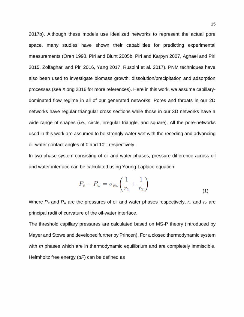
In two-phase system consisting of oil and water phases, pressure difference across oil
and water interface can be calculated using Young-Laplace equation:
(1)
Where Po and Pw are the pressures of oil and water phases respectively, r1 and r2 are
principal radii of curvature of the oil-water interface.
The threshold capillary pressures are calculated based on MS-P theory (introduced by
Mayer and Stowe and developed further by Princen). For a closed thermodynamic system
with m phases which are in thermodynamic equilibrium and are completely immiscible,
Helmholtz free energy (dF) can be defined as
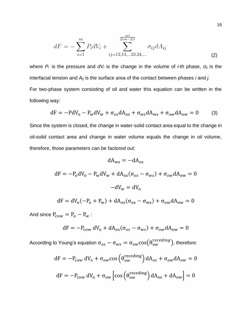
16
(2)
where Pi is the pressure and dVi is the change in the volume of i-th phase, σij is the
interfacial tension and Aij is the surface area of the contact between phases i and j.
For two-phase system consisting of oil and water this equation can be written in the
following way:
dF = −PdVo − PwdVw + σ𝑜𝑠dAos + σ𝑤𝑠dAws + σ𝑜𝑤dAow = 0 (3)
Since the system is closed, the change in water-solid contact area equal to the change in
oil-solid contact area and change in water volume equals the change in oil volume,
therefore, those parameters can be factored out:
dAws = −dAos
dF = −PodVo − PwdVw + dAos(σ𝑜𝑠 − σ𝑤𝑠) + σ𝑜𝑤dAow = 0
−dVw = dVo
dF = dVo(−Po + Pw) + dAos(σos − σws) + σowdAow = 0
And since Pcow = Po − Pw :
dF = −Pcow dVo + dAos(σ𝑜𝑠 − σ𝑤𝑠) + σ𝑜𝑤dAow = 0
According to Young’s equation σ𝑜𝑠 − σ𝑤𝑠 = σ𝑜𝑤cos(θ𝑜𝑤𝑟𝑒𝑐𝑒𝑑𝑖𝑛𝑔
), therefore:
dF = −P𝑐𝑜𝑤 dV𝑜 + σ𝑜𝑤cos (θ𝑜𝑤receding
) dA𝑜𝑠 + σ𝑜𝑤dA𝑜𝑤 = 0
dF = −Pcow dVo + σ𝑜𝑤 [cos (θ𝑜𝑤receding
) dAos + dAow] = 0

17
Since Pcow = σ𝑜w ×1
𝑟𝑜𝑤 :
(4)
The developed model in this work can be divided into two main parts: a pore network
generator and a flow simulator. This is to investigate microporosity’s impact on flow and
electrical properties using both 2- and 3-D pore networks. The 2D pore networks are
generated to interpret the results on simpler networks. We then compare our results of
3D pore networks extracted for Berea sandstone and Estaillades limestone samples.
Here, we go over our pore network modeling and generation techniques.
3.2. 2D pore networks generation
Being able to generate a random Pore-Network model allows to have control on several
geological or geometrical properties such as porosity, pore coordination number and pore
size range.
One of the main challenges in generation of random pore-network model is making it
geometrically and geologically realistic, so that lengths and radii are within pre-given
ranges and within geometrical limitations. Therefore, we generate a random pore-network
on lattice principle. All pores are located in the nodes of lattice and all throats are located
on the sides of a grid cell, thus, the network has vertical and horizontal throats.
Here, we refer to pores and throats altogether as ‘elements’. In the context of Python
code, all elements are instances of the same class named ‘Triangle’. Triangle class takes
two input parameters: inscribed radius and length. All other parameters such as threshold
18
capillary pressure and water saturation at some given capillary pressure are automatically
calculated and stored as attributes of a triangular element. Each element has inscribed
radius and length assigned to it.
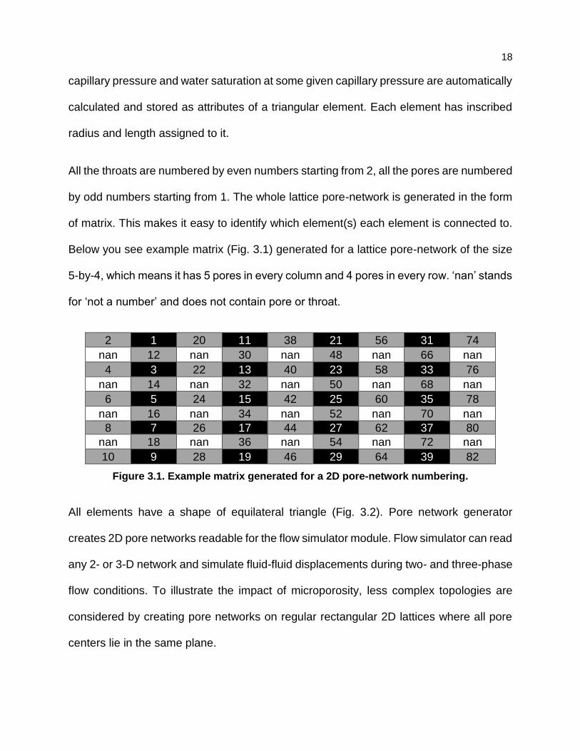
All the throats are numbered by even numbers starting from 2, all the pores are numbered
by odd numbers starting from 1. The whole lattice pore-network is generated in the form
of matrix. This makes it easy to identify which element(s) each element is connected to.
Below you see example matrix (Fig. 3.1) generated for a lattice pore-network of the size
5-by-4, which means it has 5 pores in every column and 4 pores in every row. ‘nan’ stands
for ‘not a number’ and does not contain pore or throat.
2 1 20 11 38 21 56 31 74
nan 12 nan 30 nan 48 nan 66 nan
4 3 22 13 40 23 58 33 76
nan 14 nan 32 nan 50 nan 68 nan
6 5 24 15 42 25 60 35 78
nan 16 nan 34 nan 52 nan 70 nan
8 7 26 17 44 27 62 37 80
nan 18 nan 36 nan 54 nan 72 nan
10 9 28 19 46 29 64 39 82
Figure 3.1. Example matrix generated for a 2D pore-network numbering.
All elements have a shape of equilateral triangle (Fig. 3.2). Pore network generator
creates 2D pore networks readable for the flow simulator module. Flow simulator can read
any 2- or 3-D network and simulate fluid-fluid displacements during two- and three-phase
flow conditions. To illustrate the impact of microporosity, less complex topologies are
considered by creating pore networks on regular rectangular 2D lattices where all pore
centers lie in the same plane.
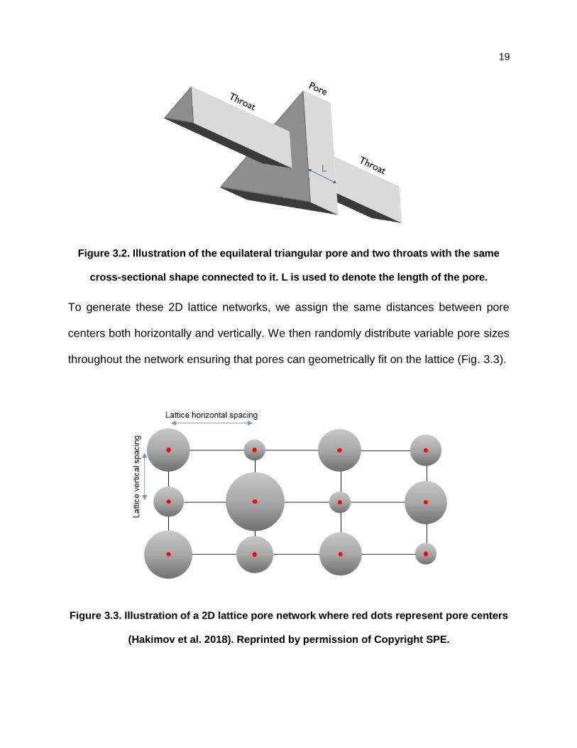
19
Figure 3.2. Illustration of the equilateral triangular pore and two throats with the same
cross-sectional shape connected to it. L is used to denote the length of the pore.
To generate these 2D lattice networks, we assign the same distances between pore
centers both horizontally and vertically. We then randomly distribute variable pore sizes
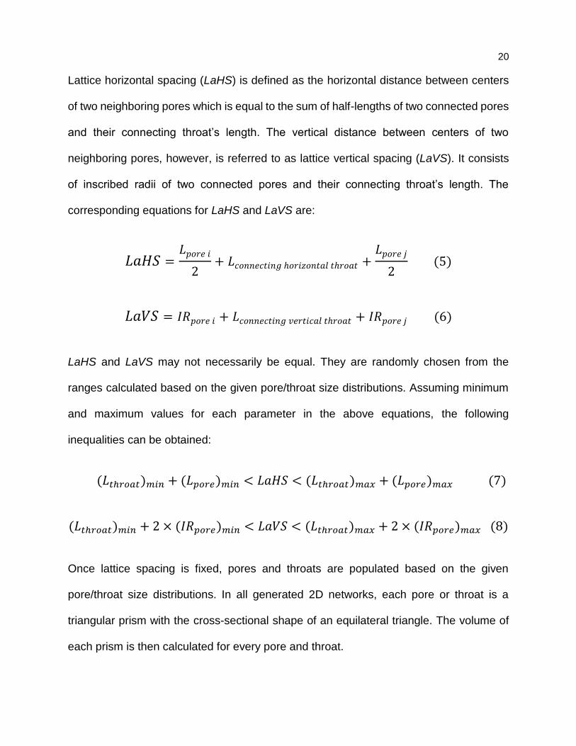
throughout the network ensuring that pores can geometrically fit on the lattice (Fig. 3.3).
Figure 3.3. Illustration of a 2D lattice pore network where red dots represent pore centers
(Hakimov et al. 2018). Reprinted by permission of Copyright SPE.
20
Lattice horizontal spacing (LaHS) is defined as the horizontal distance between centers
of two neighboring pores which is equal to the sum of half-lengths of two connected pores
and their connecting throat’s length. The vertical distance between centers of two
neighboring pores, however, is referred to as lattice vertical spacing (LaVS). It consists
of inscribed radii of two connected pores and their connecting throat’s length. The
corresponding equations for LaHS and LaVS are:
𝐿𝑎𝐻𝑆 =𝐿𝑝𝑜𝑟𝑒 𝑖
2+ 𝐿𝑐𝑜𝑛𝑛𝑒𝑐𝑡𝑖𝑛𝑔 ℎ𝑜𝑟𝑖𝑧𝑜𝑛𝑡𝑎𝑙 𝑡ℎ𝑟𝑜𝑎𝑡 +
𝐿𝑝𝑜𝑟𝑒 𝑗
2 (5)
𝐿𝑎𝑉𝑆 = 𝐼𝑅𝑝𝑜𝑟𝑒 𝑖 + 𝐿𝑐𝑜𝑛𝑛𝑒𝑐𝑡𝑖𝑛𝑔 𝑣𝑒𝑟𝑡𝑖𝑐𝑎𝑙 𝑡ℎ𝑟𝑜𝑎𝑡 + 𝐼𝑅𝑝𝑜𝑟𝑒 𝑗 (6)
LaHS and LaVS may not necessarily be equal. They are randomly chosen from the
ranges calculated based on the given pore/throat size distributions. Assuming minimum
and maximum values for each parameter in the above equations, the following
inequalities can be obtained:
(𝐿𝑡ℎ𝑟𝑜𝑎𝑡)𝑚𝑖𝑛 + (𝐿𝑝𝑜𝑟𝑒)𝑚𝑖𝑛 < 𝐿𝑎𝐻𝑆 < (𝐿𝑡ℎ𝑟𝑜𝑎𝑡)𝑚𝑎𝑥 + (𝐿𝑝𝑜𝑟𝑒)𝑚𝑎𝑥 (7)
(𝐿𝑡ℎ𝑟𝑜𝑎𝑡)𝑚𝑖𝑛 + 2 × (𝐼𝑅𝑝𝑜𝑟𝑒)𝑚𝑖𝑛 < 𝐿𝑎𝑉𝑆 < (𝐿𝑡ℎ𝑟𝑜𝑎𝑡)𝑚𝑎𝑥 + 2 × (𝐼𝑅𝑝𝑜𝑟𝑒)𝑚𝑎𝑥 (8)
Once lattice spacing is fixed, pores and throats are populated based on the given
pore/throat size distributions. In all generated 2D networks, each pore or throat is a
triangular prism with the cross-sectional shape of an equilateral triangle. The volume of
each prism is then calculated for every pore and throat.
21
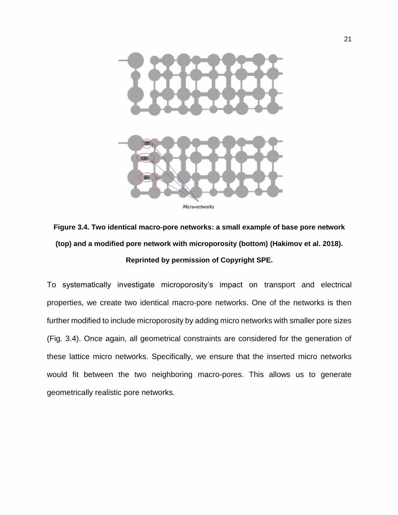
Figure 3.4. Two identical macro-pore networks: a small example of base pore network
(top) and a modified pore network with microporosity (bottom) (Hakimov et al. 2018).
Reprinted by permission of Copyright SPE.
To systematically investigate microporosity’s impact on transport and electrical
properties, we create two identical macro-pore networks. One of the networks is then
further modified to include microporosity by adding micro networks with smaller pore sizes
(Fig. 3.4). Once again, all geometrical constraints are considered for the generation of
these lattice micro networks. Specifically, we ensure that the inserted micro networks
would fit between the two neighboring macro-pores. This allows us to generate
geometrically realistic pore networks.
22
3.3. 3D pore-networks generation
3.3.1. Samples used in this work
The samples used in this work include one sandstone (Berea) and two carbonates — one
outcrop (Estaillades limestone) and one reservoir carbonate. The latter one was obtained
from the oil-producing carbonate formation of Osagean age of Mississippian period in
STACK play in Oklahoma. Conventional techniques used for water saturation calculation
yielded a high value for the considered interval. However, the Special Core Analysis
(SCAL) indicated the opposite (lower water saturation). Therefore, salinity was assumed
to be very high to increase electrical conductivity used in empirical equations which would
yield lower estimated value for water saturation. However, formation water analysis
indicated invalidity of this assumption. Thus, the company operating the field has
concluded from the well log interpretation and production tests the possibility of the
presence of the Low Resistivity Pay zone in the formation.
3.3.2. 3D Image acquisition and segmentation
Micro-CT scanner with the imaging resolution of 3.1 µm was used to obtain 3D image of
the interior of the rock sample (Fig. 3.5). X-rays pass freely through the pore space but
are absorbed or scattered by the solid (matrix). The denser the solid, the more X-rays are
attenuated. Microporous zones have smaller effective density than the regular imporous
solid parts of the sample and, therefore, are supposed to cause less attenuation of the X-
rays and appear less bright on CT-scan images. This assumption is reasonably valid for
carbonates since they are mono-mineralic rocks. The mineralogy analysis of the reservoir
carbonate sample has shown that calcite comprises approximately 97% of the sample.
23
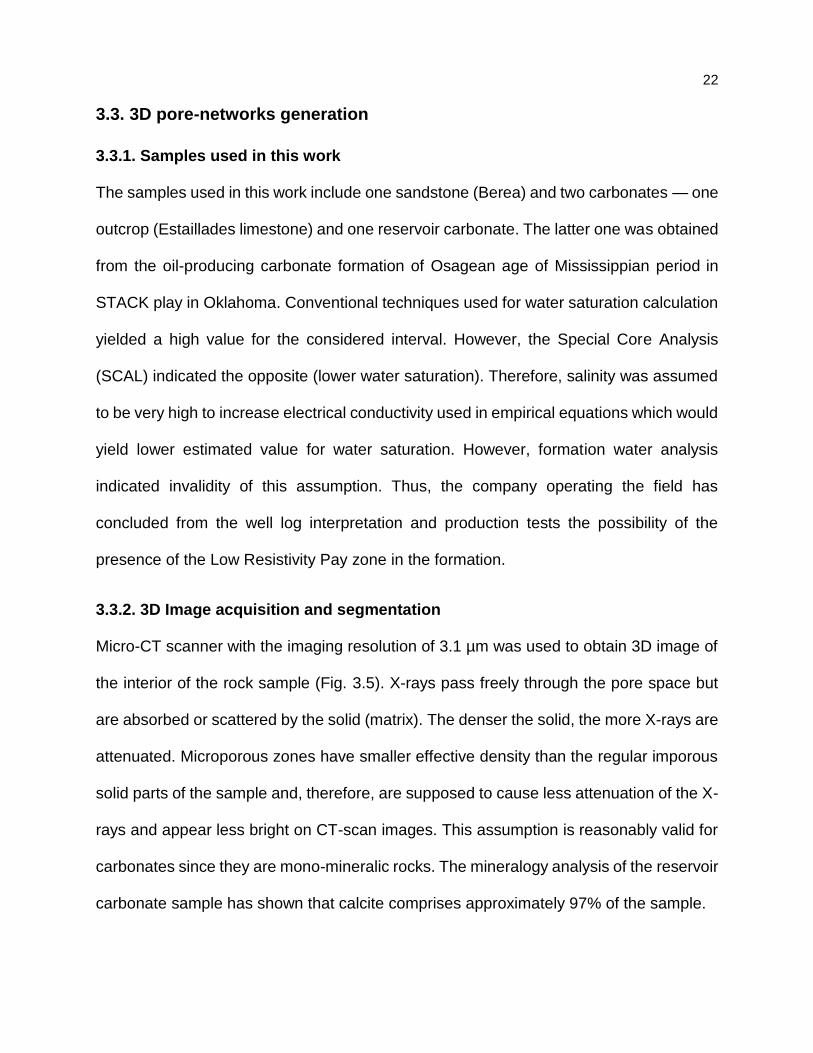
The picture below shows unsegmented, unfiltered original 3D image of the Osage
carbonate sample (Fig. 3.5. (A)). Black voxels represent resolvable pore space
(hereinafter, referred to as “macroporosity”), while dark grey ones correspond to
microporous zones, and contain pore space and solid phase at the same time. After
obtaining the 3D image of the sample, the image was filtered and segmented based on
grey level (Fig. 3.5. (B)).
Figure 3.5. The raw 3D micro-CT scan image of the sample with the resolution of 3.1 µm
(A), phases extracted the image segmentation overlaid on the original micro-CT scan
image after (B): blue color represents microporosity, red — macro pore space.
Image segmentation is a process when voxels of the image are extracted based on the
given grey level range. For this specific case, the 3D image was segmented into three
“phases”: microporosity, macro pore space and solid phase. Microporosity is assumed to
have intermediate grey level, since pore space(void) is represented by the minimum value
and the solid phase — by the maximum value of the obtained data. The Figure 1B shows
B A
24
the extracted macro pore space and microporous zones overlaid onto the original micro-
CT scan image.
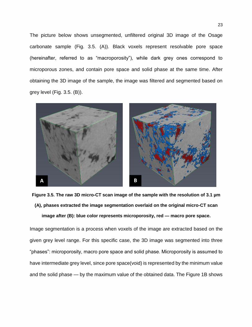
Figure 3.6. Resolved (macro) pore space (A) and its corresponding pore network where
pore and throat radii demonstrate largest inscribed radii (B).
The extracted macro space is then used to generate a macro Pore Network Model. As
can be seen from the Fig. 3.6., the significant portion of the macro pore space is
unconnected and therefore, the pore-network generation algorithm yields a large number
of isolated pores or clusters of pores. This again emphasizes the importance of inclusion
of the micro pore-networks into the model, since the individual isolated macro pores might
be connected through micro pore-network. Connection between macro and micro pores
will be referred to as ‘cross-scale’ connection and is discussed in the following subsection.
3.3.3. Stochastic pore-network generation
After the macro pore-network has been generated, the next step is to identify spatial
location and geometrical dimensions of the microporous zones. As was already
A B
25
mentioned, microporous zones are treated as a separate phase and have a separate
range of grey level which must be more than maximum grey level value of void phase
(pore space) and less than minimum one of the solid phase. Extracting the voxels in that
range, a pseudo pore space is obtained. After having the microporous media (pseudo
pore space) extracted, in an analogical way to pore-network model generation,
microporous media is converted into a network of idealized geometrical figures that would
reasonably capture the same volume and dimensions of microporous clusters, and be
located in the same geometrical domains. This network will be referred to as ‘a pseudo-
network’. Having the information on the physical dimensions, volume and location of the
elements of the pseudo-network, a special code has been developed that would
stochastically generate micro pore-network within the geometrical space occupied by the
pseudo-network (Fig. 3.7).
Figure 3.7. Illustration of a micro pore network generated within the pseudo pore space
(network).
As can be seen from the Fig. 3.8 microporous zones cover almost the whole domain of
the rock sample which indicates the high chance of them being in contact with macro
pores.
26
Figure 3.8. The segmented microporosity zone (A) and its overlay with the extracted pore
network of the resolved pore space (B).
There are many unknowns associated with microporous zones, such as porosity and pore
size distribution. Therefore, there are numerous possible networks than can be generated
within the geometrical space occupied by microporous zones.
The algorithm used in this model provides more flexibility and allows to vary various input
parameters such as pore size distribution, local porosity in microporosity zone, pore
coordination number distribution and max throat length.
In order to study the sensitivity of the results to various parameters, various micro pore-
networks have been generated with different porosities, pore size and pore coordination
number distributions. In this paper, we present the results for 15 cases with different micro
pore-networks. All these cases can be grouped based on the pore size distribution used
for microporosity zones. A group of networks with the small-sized micro pores will be
A B
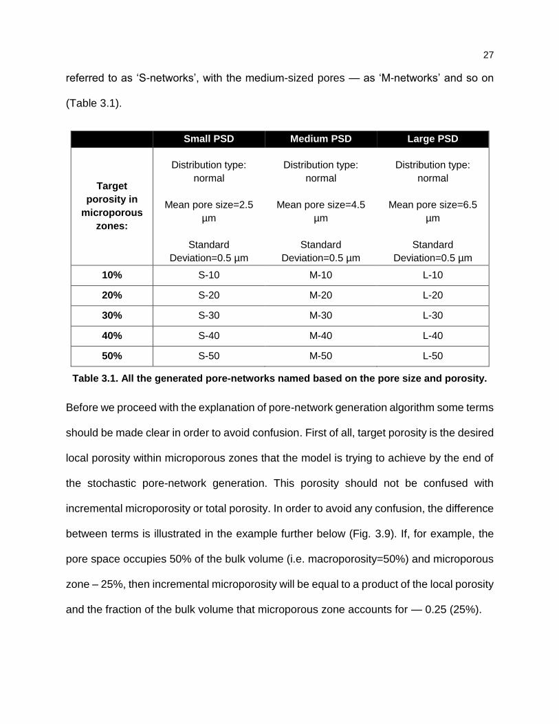
27
referred to as ‘S-networks’, with the medium-sized pores — as ‘M-networks’ and so on
(Table 3.1).
Small PSD Medium PSD Large PSD
Target
porosity in
microporous
zones:
Distribution type:
normal
Mean pore size=2.5
µm
Standard
Deviation=0.5 µm
Distribution type:
normal
Mean pore size=4.5
µm
Standard
Deviation=0.5 µm
Distribution type:
normal
Mean pore size=6.5
µm
Standard
Deviation=0.5 µm
10% S-10 M-10 L-10
20% S-20 M-20 L-20
30% S-30 M-30 L-30
40% S-40 M-40 L-40
50% S-50 M-50 L-50
Table 3.1. All the generated pore-networks named based on the pore size and porosity.
Before we proceed with the explanation of pore-network generation algorithm some terms
should be made clear in order to avoid confusion. First of all, target porosity is the desired
local porosity within microporous zones that the model is trying to achieve by the end of
the stochastic pore-network generation. This porosity should not be confused with
incremental microporosity or total porosity. In order to avoid any confusion, the difference
between terms is illustrated in the example further below (Fig. 3.9). If, for example, the
pore space occupies 50% of the bulk volume (i.e. macroporosity=50%) and microporous
zone – 25%, then incremental microporosity will be equal to a product of the local porosity
and the fraction of the bulk volume that microporous zone accounts for — 0.25 (25%).
28
Generation of a micro-network matching specific properties within specific limited
geometrical space is not a trivial task, i.e. not for any given constraints a micro-network
with the desired properties can be generated. Different cases with different pre-set input
parameters for a micro-network would involve a different set of challenges. Therefore, a
lot of these challenges are addressed in stochastic micro-network generation through
trial-and-error.
Figure 3.9. Explanation of the difference between terms ‘local porosity’ and
‘microporosity’.
The whole general workflow can be briefly described by the following steps:
1) Construction of a macro pore-network based on the pore space resolvable on 3D
image of the rock sample (Fig. 3.10(A)).
2) Extraction of the geometrical space occupied by microporosity in a form of a
network.
𝐼𝑛𝑐𝑟𝑒𝑚𝑒𝑛𝑡𝑎𝑙 𝑚𝑖𝑐𝑟𝑜𝑝𝑜𝑟𝑜𝑠𝑖𝑡𝑦 =
=𝑀𝑖𝑐𝑟𝑜 𝑝𝑜𝑟𝑒 𝑣𝑜𝑙𝑢𝑚𝑒
𝐵𝑢𝑙𝑘 𝑣𝑜𝑙𝑢𝑚𝑒=
=𝐿𝑜𝑐𝑎𝑙 𝑃𝑜𝑟𝑜𝑠𝑖𝑡𝑦 × 0.25 × 𝐵𝑢𝑙𝑘 𝑉𝑜𝑙𝑢𝑚𝑒
𝐵𝑢𝑙𝑘 𝑉𝑜𝑙𝑢𝑚𝑒=
= 𝐿𝑜𝑐𝑎𝑙 𝑃𝑜𝑟𝑜𝑠𝑖𝑡𝑦 × 0.25

29
3) Generation of the micro pores within the pseudo network based on the given target
local porosity and PSD (micro throats volumes will be considered to be negligible
and not used to match the local porosity).
4) Creating links (micro-throats) between micro-pores based on the pre-set target
pore coordination number distribution and maximum throat length. It should be
noted that before connection, a special algorithm ensures that 2 micro pores are
located in the same microporosity cluster.
5) Cross-scale connection algorithm: the code randomly generates throats between
macro pores and micro pores. However, each time, a throat connecting macro and
micro pore is being generated only in the case when the following 2 criteria are
met:
a. The micro-pore is located within microporosity cluster that is “touching” the
macro pore.
b. Adding the connection between the given micro and macro pores would not
exceed the assigned (target) coordination number for the given micro pore
(the absolute tolerance is pre-set).
c. The resulting throat length would not exceed the maximum allowed throat
length (defined as an input parameter) for micro-to-macro connection (the
relative tolerance is pre-set).
6) Continuous cluster construction algorithm checks for connectivity and identifies
isolated cluster of networks (or pores) and establishes links between the closest 2
pores of different clusters. In order to reduce computation time, a maximum length
is pre-defined for the throat connecting 2 isolated clusters.
30
Figure 3.10. Illustration of the generated macro and micro networks and their locations in
regard to the original 2D micro-CT scan image. First, an XZ-slice of the raw 3D micro-CT
scan image is shown (A), then macro pores (red) are overlaid on top of the same slice
(B). The last picture (C) shows the final network consisting of macro pores (red spheres)
and stochastically generated micro pores (grey spheres).
After all these steps, the network construction is completed, and the final information is
recorded and saved into pore-network files.
Macro
pore-
network
generated
based on the
resolvable
pore space
Based on the pre-given
input parameters,
stochastic micro pore-
network generated within
the geometrical space of
microporous zones and
linked to macro-network
A
C
B
31
3.4. Calculation of electrical properties
As mentioned, we simulate multi-phase flow under capillary-dominated flow regime. This
means that all fluid-fluid displacements are triggered by the change of capillary pressure
between displacing and displaced phases during drainage and imbibition processes. The
model calculates threshold capillary pressures of all potential displacements at each
saturation. They are then compared against the overall capillary pressure of the network
to determine occurring displacements. At each capillary pressure, after all the available
displacements are done, a quasi-steady-state condition is reached. At this condition, all
relevant transport and petrophysical properties such as water saturation, relative
permeabilities, electrical resistance or resistivity, and resistivity index are calculated.
For a detailed description of the Pore Network Models and their constituent theories, the
reader should see Piri and Blunt 2005a, Karpyn and Piri 2007, Blunt 2017, Zolfaghari and
Piri 2017a. Here in this work, we specifically improve the model of Zolfaghari and Piri
(2017a, 2017b) to estimate electrical properties in dual-porosity rock samples.
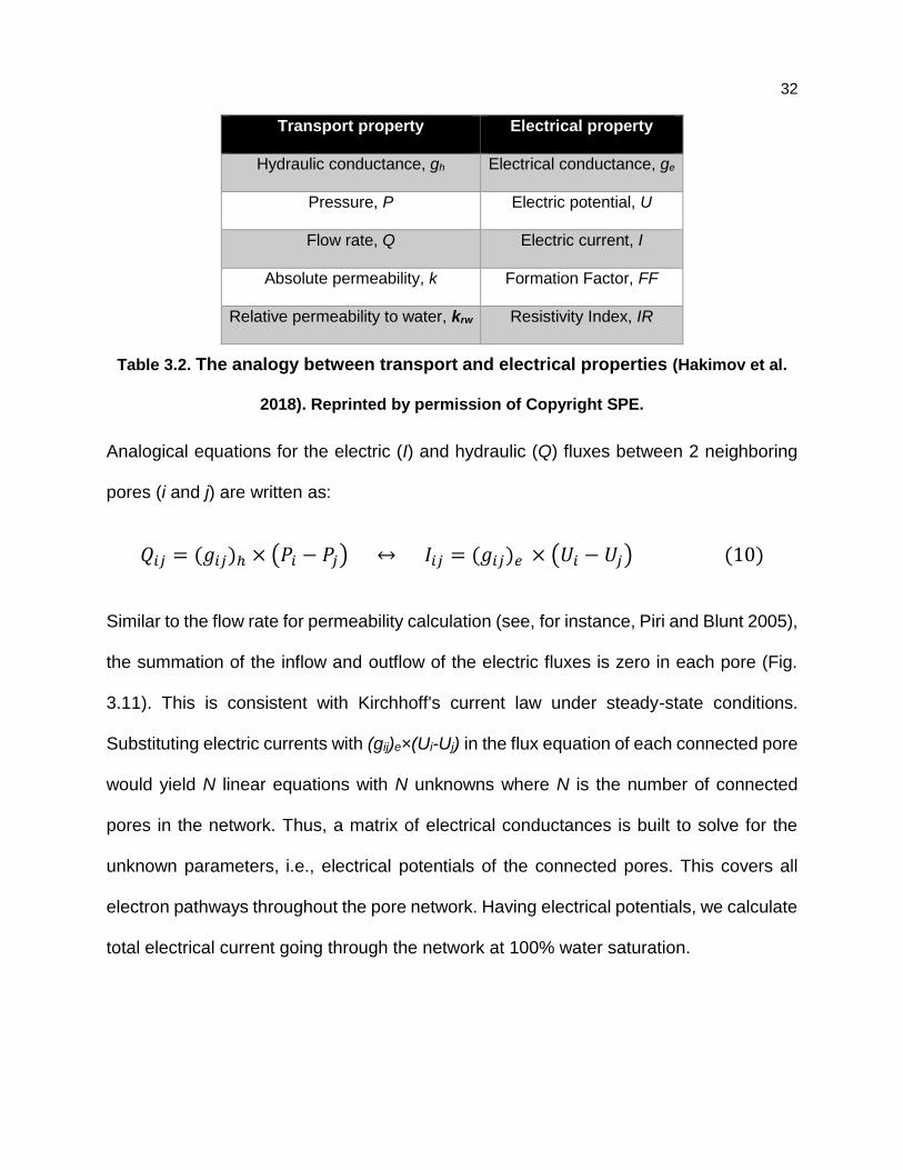
At each quasi-steady-state condition, electrical properties can be calculated in the similar
way to transport properties (Bekri et al. 2005). Each of the transport properties has an
analogical electrical parameter listed in Table 2. The analogical parameter to the hydraulic
conductance is electrical conductance which is expressed as
𝑔𝑒 = 𝜎𝑤
𝐴𝑤
𝐿 (9)
where Aw and L are water cross-sectional area and length of pore/throat, respectively. σw
denotes electrical conductivity of brine and is assumed to be 54.645 S/m (Fleury 2004).
32
Transport property Electrical property
Hydraulic conductance, gh Electrical conductance, ge
Pressure, P Electric potential, U
Flow rate, Q Electric current, I
Absolute permeability, k Formation Factor, FF
Relative permeability to water, krw Resistivity Index, IR
Table 3.2. The analogy between transport and electrical properties (Hakimov et al.
2018). Reprinted by permission of Copyright SPE.
Analogical equations for the electric (I) and hydraulic (Q) fluxes between 2 neighboring
pores (i and j) are written as:
𝑄𝑖𝑗 = (𝑔𝑖𝑗)ℎ × (𝑃𝑖 − 𝑃𝑗) ↔ 𝐼𝑖𝑗 = (𝑔𝑖𝑗)𝑒 × (𝑈𝑖 − 𝑈𝑗) (10)
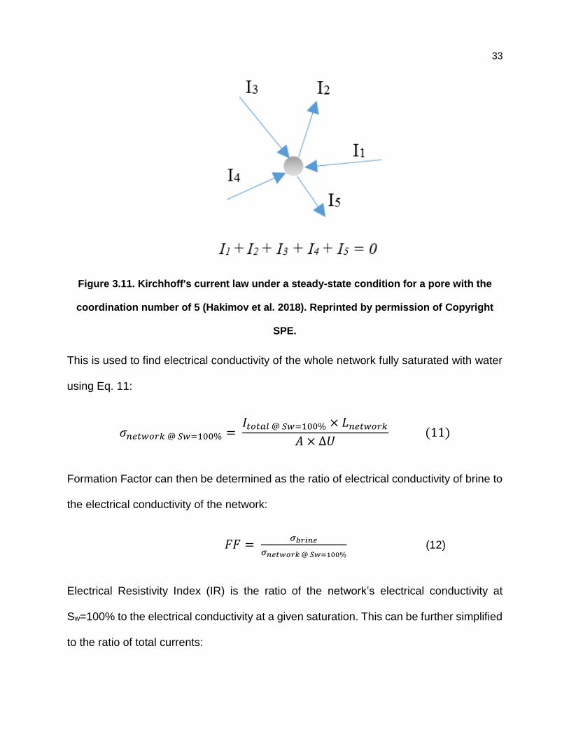
Similar to the flow rate for permeability calculation (see, for instance, Piri and Blunt 2005),
the summation of the inflow and outflow of the electric fluxes is zero in each pore (Fig.
3.11). This is consistent with Kirchhoff's current law under steady-state conditions.
Substituting electric currents with (gij)e×(Ui-Uj) in the flux equation of each connected pore
would yield N linear equations with N unknowns where N is the number of connected
pores in the network. Thus, a matrix of electrical conductances is built to solve for the
unknown parameters, i.e., electrical potentials of the connected pores. This covers all
electron pathways throughout the pore network. Having electrical potentials, we calculate
total electrical current going through the network at 100% water saturation.
33
Figure 3.11. Kirchhoff's current law under a steady-state condition for a pore with the
coordination number of 5 (Hakimov et al. 2018). Reprinted by permission of Copyright
SPE.
This is used to find electrical conductivity of the whole network fully saturated with water
using Eq. 11:
𝜎𝑛𝑒𝑡𝑤𝑜𝑟𝑘 @ 𝑆𝑤=100% = 𝐼𝑡𝑜𝑡𝑎𝑙 @ 𝑆𝑤=100% × 𝐿𝑛𝑒𝑡𝑤𝑜𝑟𝑘
𝐴 × ∆𝑈 (11)
Formation Factor can then be determined as the ratio of electrical conductivity of brine to
the electrical conductivity of the network:
𝐹𝐹 = 𝜎𝑏𝑟𝑖𝑛𝑒
𝜎𝑛𝑒𝑡𝑤𝑜𝑟𝑘 @ 𝑆𝑤=100% (12)
Electrical Resistivity Index (IR) is the ratio of the network’s electrical conductivity at
Sw=100% to the electrical conductivity at a given saturation. This can be further simplified
to the ratio of total currents:
34
𝐼𝑅 =𝜎𝑛𝑒𝑡𝑤𝑜𝑟𝑘 @ 𝑆𝑤=100%
𝜎𝑎𝑡 𝑔𝑖𝑣𝑒𝑛 𝑆𝑤
= 𝐼𝑡𝑜𝑡𝑎𝑙 @ 𝑆𝑤=100% × 𝐿𝑛𝑒𝑡𝑤𝑜𝑟𝑘
𝐴 × ∆𝑈×
𝐴 × ∆𝑈
𝐼𝑡𝑜𝑡𝑎𝑙 𝑎𝑡 𝑔𝑖𝑣𝑒𝑛 𝑆𝑤 × 𝐿𝑛𝑒𝑡𝑤𝑜𝑟𝑘=
=𝐼𝑡𝑜𝑡𝑎𝑙 @ 𝑆𝑤=100%
𝐼𝑡𝑜𝑡𝑎𝑙 𝑎𝑡 𝑔𝑖𝑣𝑒𝑛 𝑆𝑤 (13)
As mentioned, we generate networks of the same lengths and cross-sectional areas to
investigate the impact of microporosity. Having networks with the same spatial
dimensions, it is sufficient to compare only electrical conductances (𝑔𝑒) or resistances (R)
rather than conductivities (σ) or resistivities (ρ). The corresponding equations are
presented below to further illustrate such reasoning:
𝜎𝑛𝑒𝑡𝑤𝑜𝑟𝑘 = 𝐼𝑡𝑜𝑡𝑎𝑙
∆𝑈×
𝐿𝑛𝑒𝑡𝑤𝑜𝑟𝑘
𝐴 (𝑔𝑒)𝑛𝑒𝑡𝑤𝑜𝑟𝑘 =
𝐼𝑡𝑜𝑡𝑎𝑙
∆𝑈 (14)
𝜌𝑛𝑒𝑡𝑤𝑜𝑟𝑘 = ∆𝑈
𝐼𝑡𝑜𝑡𝑎𝑙×
𝐴
𝐿𝑛𝑒𝑡𝑤𝑜𝑟𝑘 𝑅𝑛𝑒𝑡𝑤𝑜𝑟𝑘 =
∆𝑈
𝐼𝑡𝑜𝑡𝑎𝑙 (15)
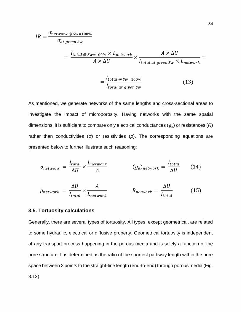
3.5. Tortuosity calculations
Generally, there are several types of tortuosity. All types, except geometrical, are related
to some hydraulic, electrical or diffusive property. Geometrical tortuosity is independent
of any transport process happening in the porous media and is solely a function of the
pore structure. It is determined as the ratio of the shortest pathway length within the pore
space between 2 points to the straight-line length (end-to-end) through porous media (Fig.
3.12).
35
Figure 3.12. Geometrical tortuosity is calculated as the ratio of the shortest pathway
length to the straight-line (end-to-end) length.
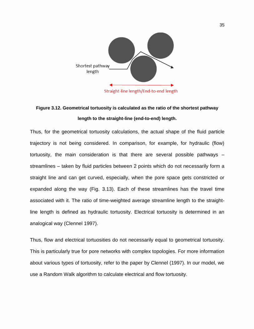
Thus, for the geometrical tortuosity calculations, the actual shape of the fluid particle
trajectory is not being considered. In comparison, for example, for hydraulic (flow)
tortuosity, the main consideration is that there are several possible pathways –
streamlines – taken by fluid particles between 2 points which do not necessarily form a
straight line and can get curved, especially, when the pore space gets constricted or
expanded along the way (Fig. 3.13). Each of these streamlines has the travel time
associated with it. The ratio of time-weighted average streamline length to the straight-
line length is defined as hydraulic tortuosity. Electrical tortuosity is determined in an
analogical way (Clennel 1997).
Thus, flow and electrical tortuosities do not necessarily equal to geometrical tortuosity.
This is particularly true for pore networks with complex topologies. For more information
about various types of tortuosity, refer to the paper by Clennel (1997). In our model, we
use a Random Walk algorithm to calculate electrical and flow tortuosity.
36
Figure 3.13. Illustration of the difference between geometrical and hydraulic tortuosity.
For the same porous media, the left picture depicts the shortest pathway length used for
geometrical tortuosity calculation, the right picture shows converging-diverging
streamlines that are considered for hydraulic tortuosity calculation.
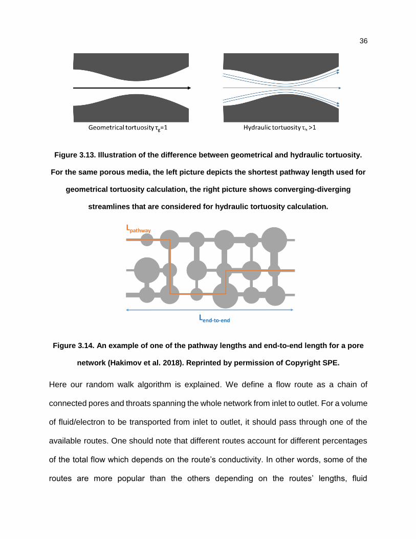
Figure 3.14. An example of one of the pathway lengths and end-to-end length for a pore
network (Hakimov et al. 2018). Reprinted by permission of Copyright SPE.
Here our random walk algorithm is explained. We define a flow route as a chain of
connected pores and throats spanning the whole network from inlet to outlet. For a volume
of fluid/electron to be transported from inlet to outlet, it should pass through one of the
available routes. One should note that different routes account for different percentages
of the total flow which depends on the route’s conductivity. In other words, some of the
routes are more popular than the others depending on the routes’ lengths, fluid
37
occupancies, and sizes of the constituent pores and throats. It is computationally
infeasible to identify all possible pathways and calculate percentages of the total flow for
each of them. Therefore, it is rational to calculate the average length of many particles
traversing from inlet to outlet. To obtain reliable results, the number of particles should be
high enough depending on the topology and connectivity of the pore network. A Random
Walk algorithm is developed to simulate the movement of each particle. Initially, all
particles enter the network from the inlet side. Giving more chances to throats with higher
flow rates, each particle is then randomly assigned to an inlet throat. The particle then
moves to the pore connected to the given inlet throat. Further, the particle can travel to
any neighboring connected pore(s) that has lower pressure (or electric potential) than that
of the current pore. If there is more than one option, the particle’s trajectory is randomly
chosen based on the throats’ flow rates (or electric currents) that are connecting various
destination pores. Once the particle reaches the outlet, the transversed trajectory is
calculated. Repeating such calculations for many particles, the average pathway length
is calculated. Tortuosity is then determined as the ratio of the average pathway length to
the straight line (end-to-end) length of the network. (Fig. 3.14).
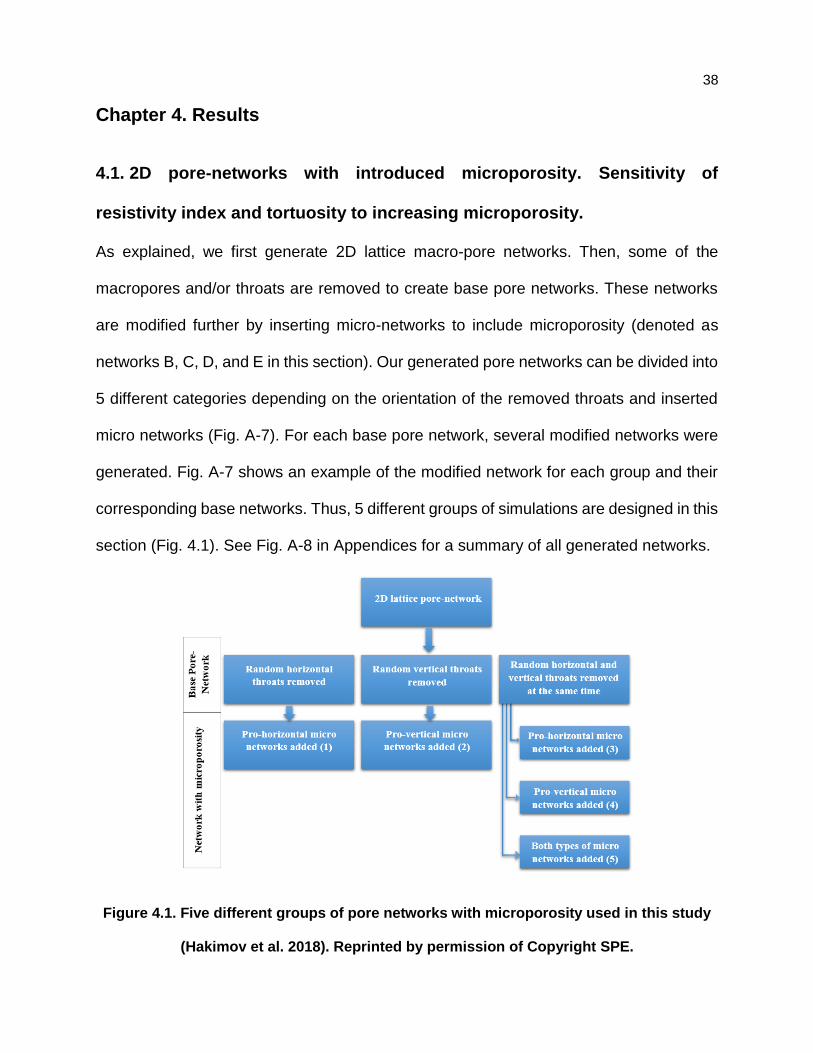
38
Chapter 4. Results
4.1. 2D pore-networks with introduced microporosity. Sensitivity of
resistivity index and tortuosity to increasing microporosity.
As explained, we first generate 2D lattice macro-pore networks. Then, some of the
macropores and/or throats are removed to create base pore networks. These networks
are modified further by inserting micro-networks to include microporosity (denoted as
networks B, C, D, and E in this section). Our generated pore networks can be divided into
5 different categories depending on the orientation of the removed throats and inserted
micro networks (Fig. A-7). For each base pore network, several modified networks were
generated. Fig. A-7 shows an example of the modified network for each group and their
corresponding base networks. Thus, 5 different groups of simulations are designed in this
section (Fig. 4.1). See Fig. A-8 in Appendices for a summary of all generated networks.
Figure 4.1. Five different groups of pore networks with microporosity used in this study
(Hakimov et al. 2018). Reprinted by permission of Copyright SPE.
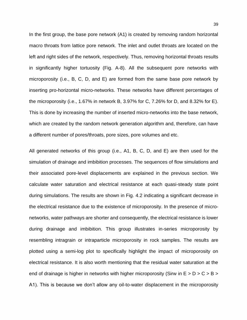
39
In the first group, the base pore network (A1) is created by removing random horizontal
macro throats from lattice pore network. The inlet and outlet throats are located on the
left and right sides of the network, respectively. Thus, removing horizontal throats results
in significantly higher tortuosity (Fig. A-8). All the subsequent pore networks with
microporosity (i.e., B, C, D, and E) are formed from the same base pore network by
inserting pro-horizontal micro-networks. These networks have different percentages of
the microporosity (i.e., 1.67% in network B, 3.97% for C, 7.26% for D, and 8.32% for E).
This is done by increasing the number of inserted micro-networks into the base network,
which are created by the random network generation algorithm and, therefore, can have
a different number of pores/throats, pore sizes, pore volumes and etc.
All generated networks of this group (i.e., A1, B, C, D, and E) are then used for the
simulation of drainage and imbibition processes. The sequences of flow simulations and
their associated pore-level displacements are explained in the previous section. We
calculate water saturation and electrical resistance at each quasi-steady state point
during simulations. The results are shown in Fig. 4.2 indicating a significant decrease in
the electrical resistance due to the existence of microporosity. In the presence of micro-
networks, water pathways are shorter and consequently, the electrical resistance is lower
during drainage and imbibition. This group illustrates in-series microporosity by
resembling intragrain or intraparticle microporosity in rock samples. The results are
plotted using a semi-log plot to specifically highlight the impact of microporosity on
electrical resistance. It is also worth mentioning that the residual water saturation at the
end of drainage is higher in networks with higher microporosity (Sirw in E > D > C > B >
A1). This is because we don’t allow any oil-to-water displacement in the microporosity
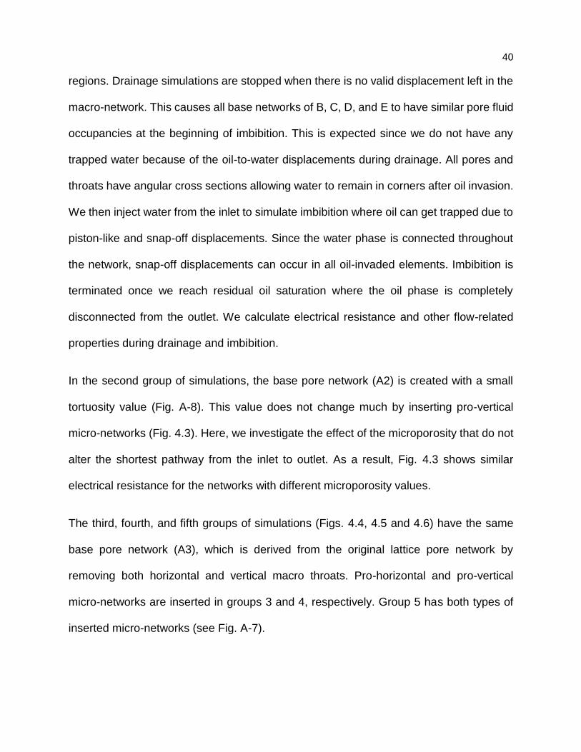
40
regions. Drainage simulations are stopped when there is no valid displacement left in the
macro-network. This causes all base networks of B, C, D, and E to have similar pore fluid
occupancies at the beginning of imbibition. This is expected since we do not have any
trapped water because of the oil-to-water displacements during drainage. All pores and
throats have angular cross sections allowing water to remain in corners after oil invasion.
We then inject water from the inlet to simulate imbibition where oil can get trapped due to
piston-like and snap-off displacements. Since the water phase is connected throughout
the network, snap-off displacements can occur in all oil-invaded elements. Imbibition is
terminated once we reach residual oil saturation where the oil phase is completely
disconnected from the outlet. We calculate electrical resistance and other flow-related
properties during drainage and imbibition.
In the second group of simulations, the base pore network (A2) is created with a small
tortuosity value (Fig. A-8). This value does not change much by inserting pro-vertical
micro-networks (Fig. 4.3). Here, we investigate the effect of the microporosity that do not
alter the shortest pathway from the inlet to outlet. As a result, Fig. 4.3 shows similar
electrical resistance for the networks with different microporosity values.
The third, fourth, and fifth groups of simulations (Figs. 4.4, 4.5 and 4.6) have the same
base pore network (A3), which is derived from the original lattice pore network by
removing both horizontal and vertical macro throats. Pro-horizontal and pro-vertical
micro-networks are inserted in groups 3 and 4, respectively. Group 5 has both types of
inserted micro-networks (see Fig. A-7).
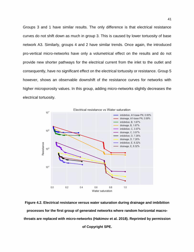
41
Groups 3 and 1 have similar results. The only difference is that electrical resistance
curves do not shift down as much in group 3. This is caused by lower tortuosity of base
network A3. Similarly, groups 4 and 2 have similar trends. Once again, the introduced
pro-vertical micro-networks have only a volumetrical effect on the results and do not
provide new shorter pathways for the electrical current from the inlet to the outlet and
consequently, have no significant effect on the electrical tortuosity or resistance. Group 5
however, shows an observable downshift of the resistance curves for networks with
higher microporosity values. In this group, adding micro-networks slightly decreases the
electrical tortuosity.
Figure 4.2. Electrical resistance versus water saturation during drainage and imbibition
processes for the first group of generated networks where random horizontal macro-
throats are replaced with micro-networks (Hakimov et al. 2018). Reprinted by permission
of Copyright SPE.
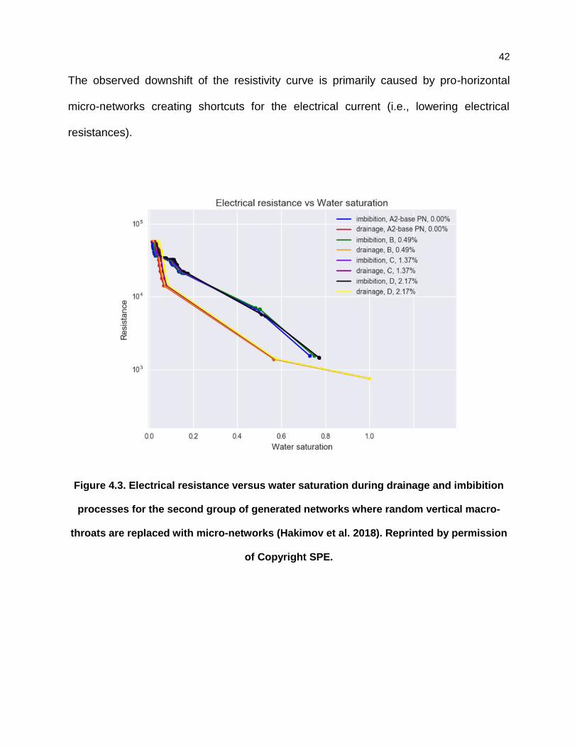
42
The observed downshift of the resistivity curve is primarily caused by pro-horizontal
micro-networks creating shortcuts for the electrical current (i.e., lowering electrical
resistances).
Figure 4.3. Electrical resistance versus water saturation during drainage and imbibition
processes for the second group of generated networks where random vertical macro-
throats are replaced with micro-networks (Hakimov et al. 2018). Reprinted by permission
of Copyright SPE.
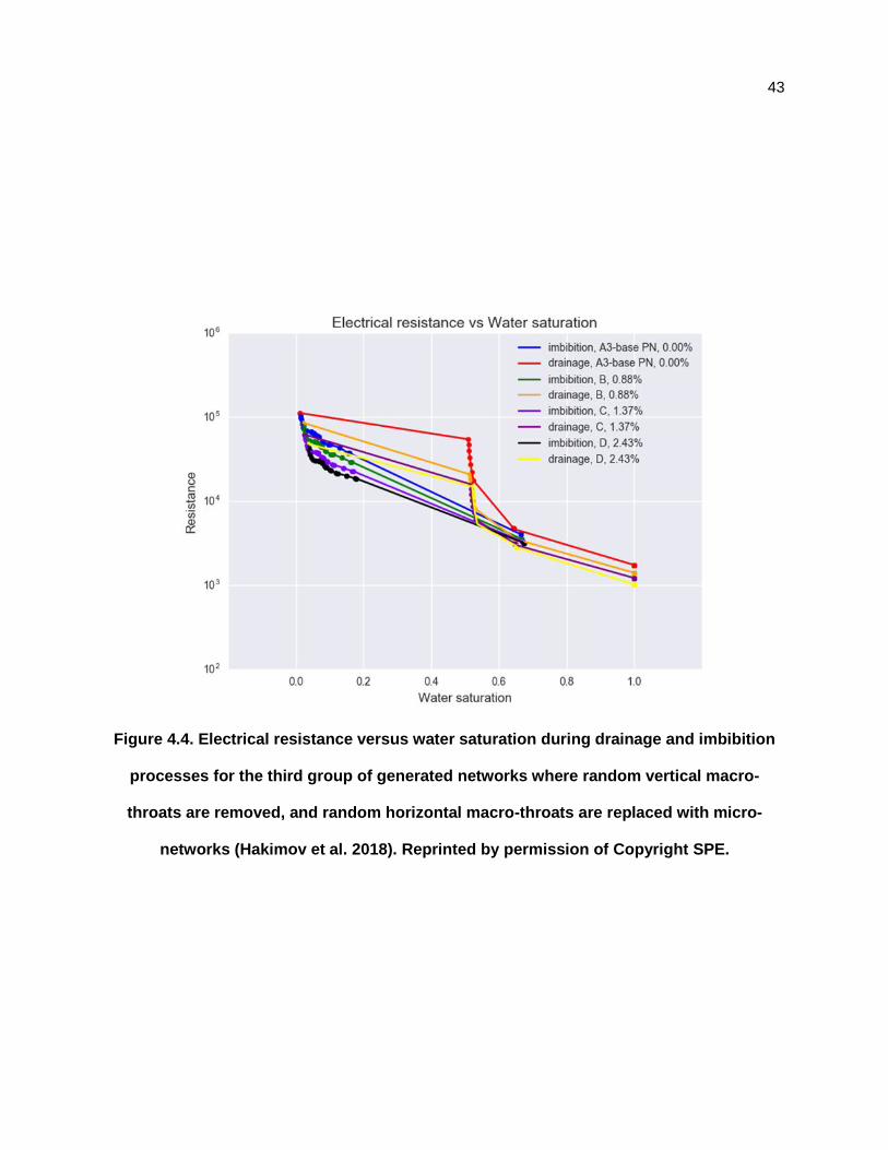
43
Figure 4.4. Electrical resistance versus water saturation during drainage and imbibition
processes for the third group of generated networks where random vertical macro-
throats are removed, and random horizontal macro-throats are replaced with micro-
networks (Hakimov et al. 2018). Reprinted by permission of Copyright SPE.
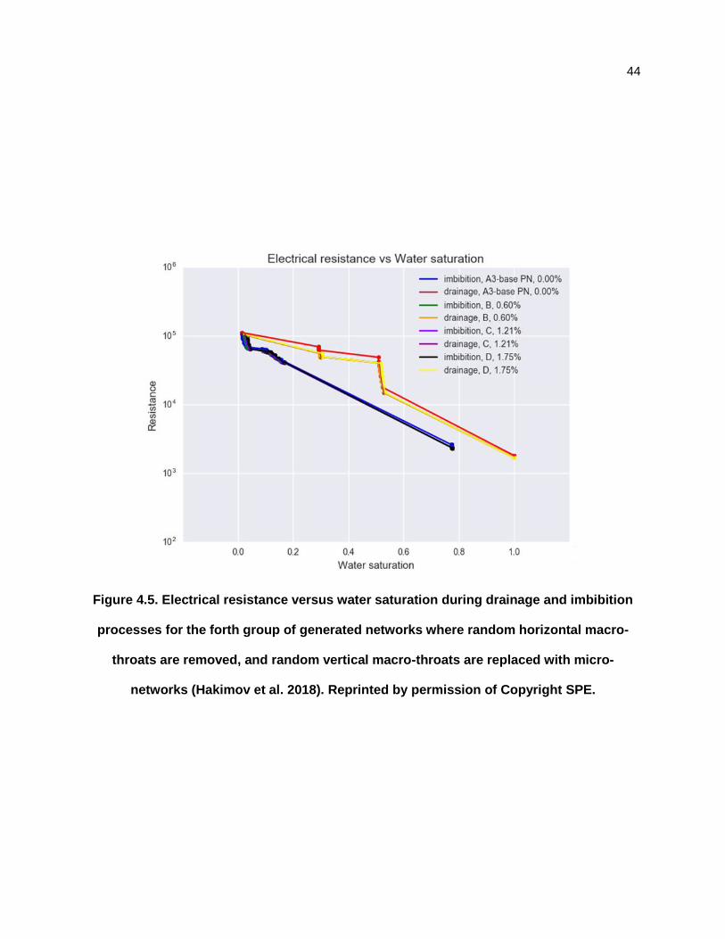
44
Figure 4.5. Electrical resistance versus water saturation during drainage and imbibition
processes for the forth group of generated networks where random horizontal macro-
throats are removed, and random vertical macro-throats are replaced with micro-
networks (Hakimov et al. 2018). Reprinted by permission of Copyright SPE.
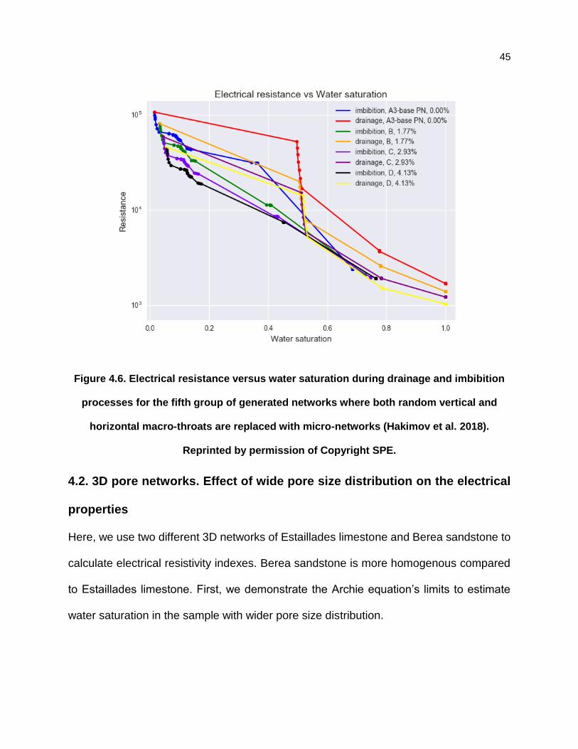
45
Figure 4.6. Electrical resistance versus water saturation during drainage and imbibition
processes for the fifth group of generated networks where both random vertical and
horizontal macro-throats are replaced with micro-networks (Hakimov et al. 2018).
Reprinted by permission of Copyright SPE.
4.2. 3D pore networks. Effect of wide pore size distribution on the electrical
properties
Here, we use two different 3D networks of Estaillades limestone and Berea sandstone to
calculate electrical resistivity indexes. Berea sandstone is more homogenous compared
to Estaillades limestone. First, we demonstrate the Archie equation’s limits to estimate
water saturation in the sample with wider pore size distribution.
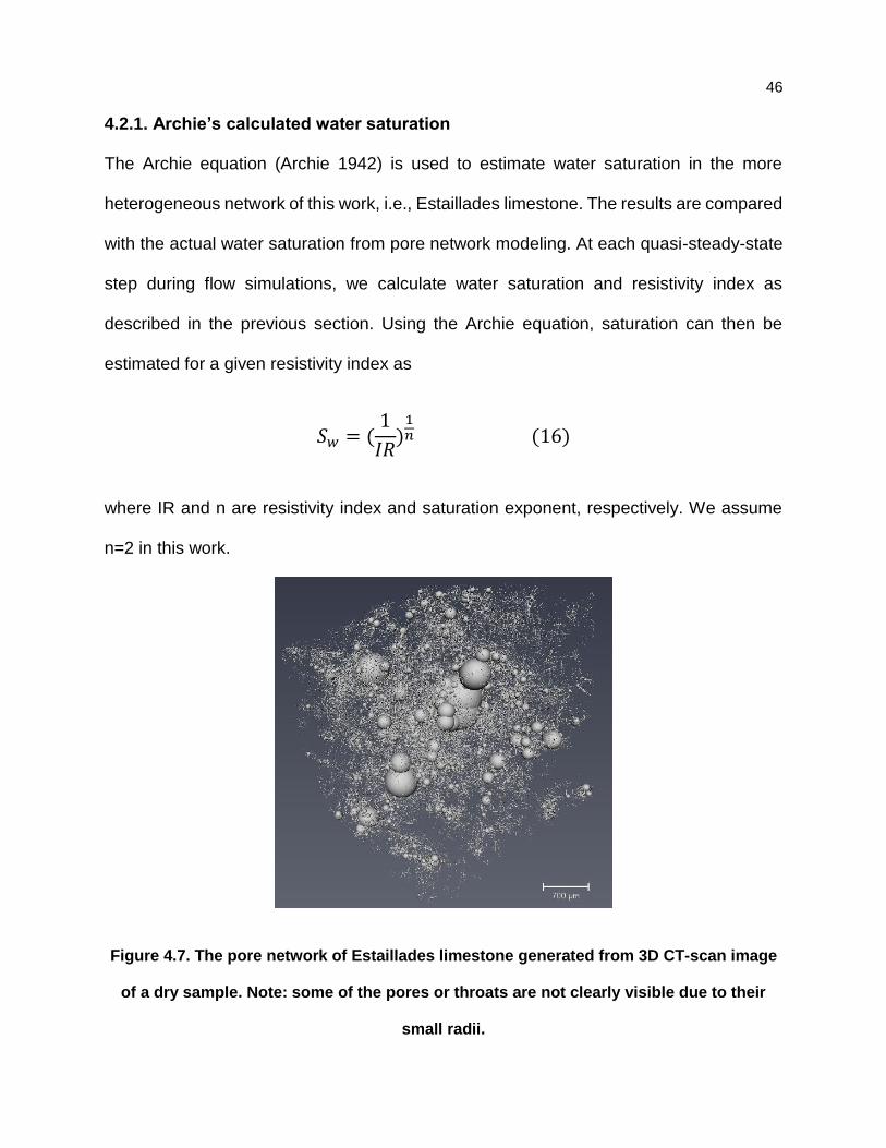
46
4.2.1. Archie’s calculated water saturation
The Archie equation (Archie 1942) is used to estimate water saturation in the more
heterogeneous network of this work, i.e., Estaillades limestone. The results are compared
with the actual water saturation from pore network modeling. At each quasi-steady-state
step during flow simulations, we calculate water saturation and resistivity index as
described in the previous section. Using the Archie equation, saturation can then be
estimated for a given resistivity index as
𝑆𝑤 = (1
𝐼𝑅)
1𝑛 (16)
where IR and n are resistivity index and saturation exponent, respectively. We assume
n=2 in this work.
Figure 4.7. The pore network of Estaillades limestone generated from 3D CT-scan image
of a dry sample. Note: some of the pores or throats are not clearly visible due to their
small radii.

47
We used 3D CT-scan image of Estaillades limestone with 3.1-µm resolution (Bultreys et
al. 2016) to extract the representative pore network. To do so, the Thermo Fisher
Scientific™ PerGeos™ software package is used to extract the pore space from images,
perform connectivity analysis, skeletonization, and clustering, and finally assign
geometric properties to all generated pores and throats. Fig. 4.7 shows the representative
pore network of the entire image volume (i.e., a cube with the dimensions 3096.9 μm ×
3096.9 μm × 3100 μm). This network has 126586 pores and 316192 throats which is too
large for our flow simulation. Therefore, a small sub-volume of the original image is used
to generate a pore network for the simulation of drainage and imbibition flow cycles.
Similar to the 2D networks, we assign equilateral triangles for the cross section of all
pores and throats. The resistivity index during drainage is plotted in Fig. 4.8. The results
indicate that the Archie equation fairly predicts intermediate and high water saturation but
overestimates lower water saturation regions.
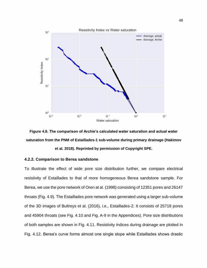
48
Figure 4.8. The comparison of Archie’s calculated water saturation and actual water
saturation from the PNM of Estaillades-1 sub-volume during primary drainage (Hakimov
et al. 2018). Reprinted by permission of Copyright SPE.
4.2.2. Comparison to Berea sandstone
To illustrate the effect of wide pore size distribution further, we compare electrical
resistivity of Estaillades to that of more homogeneous Berea sandstone sample. For
Berea, we use the pore network of Oren at al. (1998) consisting of 12351 pores and 26147
throats (Fig. 4.9). The Estaillades pore network was generated using a larger sub-volume
of the 3D images of Bultreys et al. (2016), i.e., Estaillades-2. It consists of 25718 pores
and 45904 throats (see Fig. 4.10 and Fig. A-9 in the Appendices). Pore size distributions
of both samples are shown in Fig. 4.11. Resistivity indices during drainage are plotted in
Fig. 4.12. Berea’s curve forms almost one single slope while Estaillades shows drastic
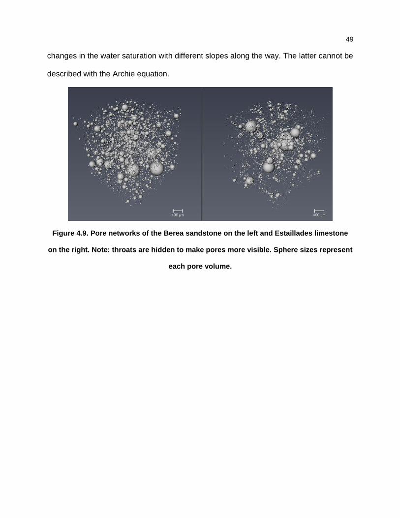
49
changes in the water saturation with different slopes along the way. The latter cannot be
described with the Archie equation.
Figure 4.9. Pore networks of the Berea sandstone on the left and Estaillades limestone
on the right. Note: throats are hidden to make pores more visible. Sphere sizes represent
each pore volume.
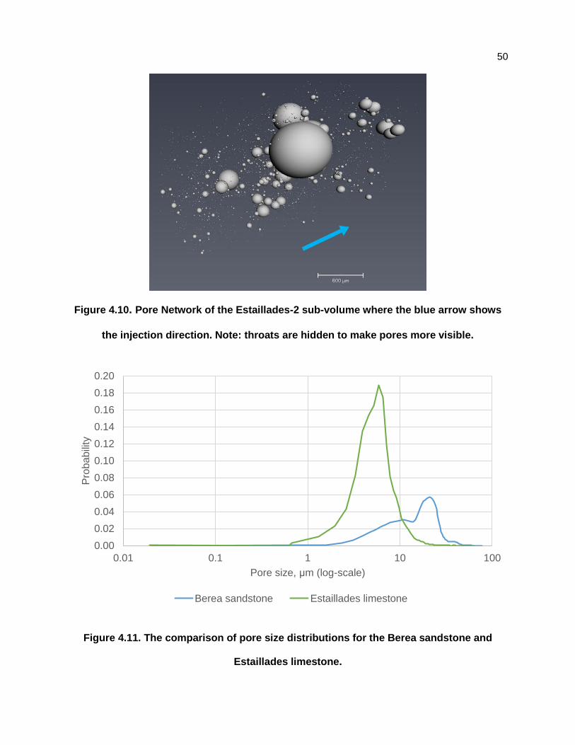
50
Figure 4.10. Pore Network of the Estaillades-2 sub-volume where the blue arrow shows
the injection direction. Note: throats are hidden to make pores more visible.
Figure 4.11. The comparison of pore size distributions for the Berea sandstone and
Estaillades limestone.
0.00
0.02
0.04
0.06
0.08
0.10
0.12
0.14
0.16
0.18
0.20
0.01 0.1 1 10 100
Pro
ba
bili
ty
Pore size, μm (log-scale)
Berea sandstone Estaillades limestone
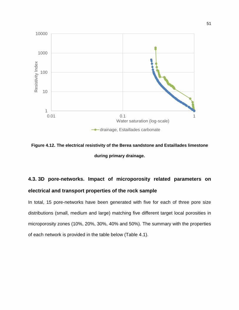
51
Figure 4.12. The electrical resistivity of the Berea sandstone and Estaillades limestone
during primary drainage.
4.3. 3D pore-networks. Impact of microporosity related parameters on
electrical and transport properties of the rock sample
In total, 15 pore-networks have been generated with five for each of three pore size
distributions (small, medium and large) matching five different target local porosities in
microporosity zones (10%, 20%, 30%, 40% and 50%). The summary with the properties
of each network is provided in the table below (Table 4.1).
1
10
100
1000
10000
0.01 0.1 1
Re
sis
tivity I
nde
x
Water saturation (log-scale)
drainage, Estaillades carbonate
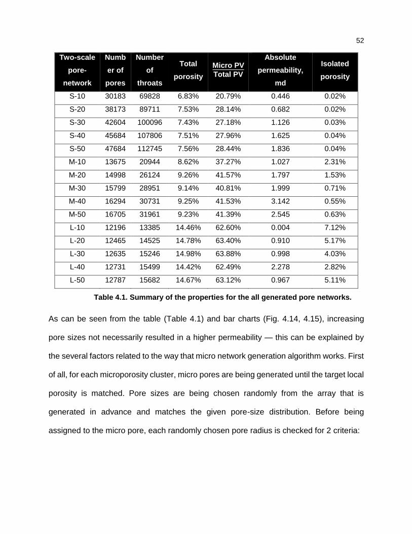
52
Two-scale
pore-
network
Numb
er of
pores
Number
of
throats
Total
porosity
Micro PV
Total PV
Absolute
permeability,
md
Isolated
porosity
S-10 30183 69828 6.83% 20.79% 0.446 0.02%
S-20 38173 89711 7.53% 28.14% 0.682 0.02%
S-30 42604 100096 7.43% 27.18% 1.126 0.03%
S-40 45684 107806 7.51% 27.96% 1.625 0.04%
S-50 47684 112745 7.56% 28.44% 1.836 0.04%
M-10 13675 20944 8.62% 37.27% 1.027 2.31%
M-20 14998 26124 9.26% 41.57% 1.797 1.53%
M-30 15799 28951 9.14% 40.81% 1.999 0.71%
M-40 16294 30731 9.25% 41.53% 3.142 0.55%
M-50 16705 31961 9.23% 41.39% 2.545 0.63%
L-10 12196 13385 14.46% 62.60% 0.004 7.12%
L-20 12465 14525 14.78% 63.40% 0.910 5.17%
L-30 12635 15246 14.98% 63.88% 0.998 4.03%
L-40 12731 15499 14.42% 62.49% 2.278 2.82%
L-50 12787 15682 14.67% 63.12% 0.967 5.11%
Table 4.1. Summary of the properties for the all generated pore networks.
As can be seen from the table (Table 4.1) and bar charts (Fig. 4.14, 4.15), increasing
pore sizes not necessarily resulted in a higher permeability — this can be explained by
the several factors related to the way that micro network generation algorithm works. First
of all, for each microporosity cluster, micro pores are being generated until the target local
porosity is matched. Pore sizes are being chosen randomly from the array that is
generated in advance and matches the given pore-size distribution. Before being
assigned to the micro pore, each randomly chosen pore radius is checked for 2 criteria:

53
1) It should geometrically fit the given microporosity cluster, i.e. not exceed
dimensions of the given space occupied by microporosity (the pre-set relative
tolerance should not be exceeded).
2) Adding the given pore radius should not result in the local porosity greater than the
target value (similarly, the relative tolerance is checked).
If any of these conditions is not satisfied, the randomly chosen pore size will not be added
to the network. In that case, another random choice will be made. In case there is no pore
size in the pre-generated pore-size distribution that would match these criteria, no pore
will be created.
Therefore, depending on the available pore size options and how close the current local
porosity (after creating some number of micro pores) is to the target value, a pore might
be generated or not generated at all. This means that in the same cross-section of the
sample’s cubic domain there might be less pore area open to flow in the L-networks than
in the S-networks. In case with the large pore size distribution (the same as with the
medium distribution in comparison with the small one), execution of the algorithm results
in generating fewer number of pores leading to a smaller area open to the flow. However,
this is not the sole contributor leading to these results. The second important factor is
poorer pore connectivity of the L-networks in comparison with the S-networks. As can be
seen from the graph (Fig. 4.13), L-10 has significantly higher number of pores with the
coordination number of 1, while S-10 has the mean coordination number of 5. In other
words, there are higher number of ‘dead-end’ or ‘cul-de-sac’ pores in L-10 than in S-10.
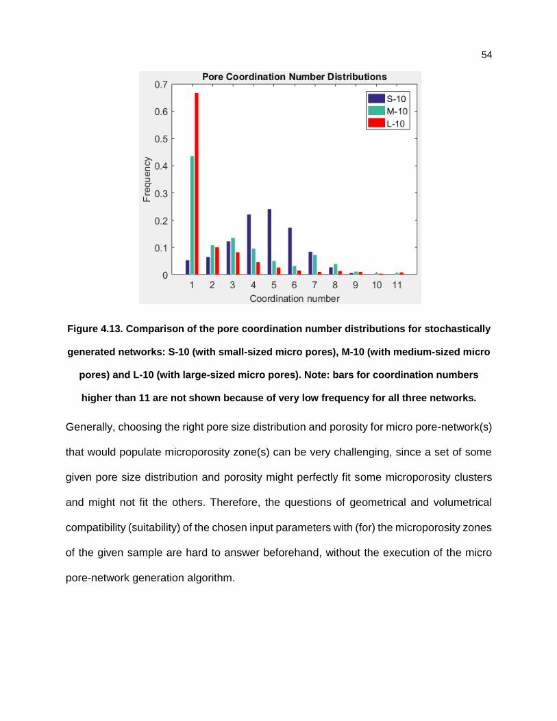
54
Figure 4.13. Comparison of the pore coordination number distributions for stochastically
generated networks: S-10 (with small-sized micro pores), M-10 (with medium-sized micro
pores) and L-10 (with large-sized micro pores). Note: bars for coordination numbers
higher than 11 are not shown because of very low frequency for all three networks.
Generally, choosing the right pore size distribution and porosity for micro pore-network(s)
that would populate microporosity zone(s) can be very challenging, since a set of some
given pore size distribution and porosity might perfectly fit some microporosity clusters
and might not fit the others. Therefore, the questions of geometrical and volumetrical
compatibility (suitability) of the chosen input parameters with (for) the microporosity zones
of the given sample are hard to answer beforehand, without the execution of the micro
pore-network generation algorithm.
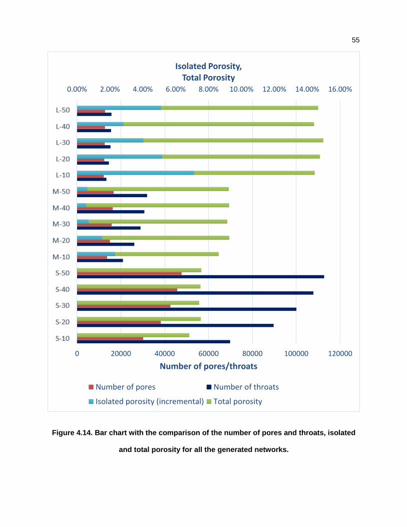
55
Figure 4.14. Bar chart with the comparison of the number of pores and throats, isolated
and total porosity for all the generated networks.
0.00% 2.00% 4.00% 6.00% 8.00% 10.00% 12.00% 14.00% 16.00%
0 20000 40000 60000 80000 100000 120000
S-10
S-20
S-30
S-40
S-50
M-10
M-20
M-30
M-40
M-50
L-10
L-20
L-30
L-40
L-50
Isolated Porosity,Total Porosity
Number of pores/throats
Number of pores Number of throats
Isolated porosity (incremental) Total porosity
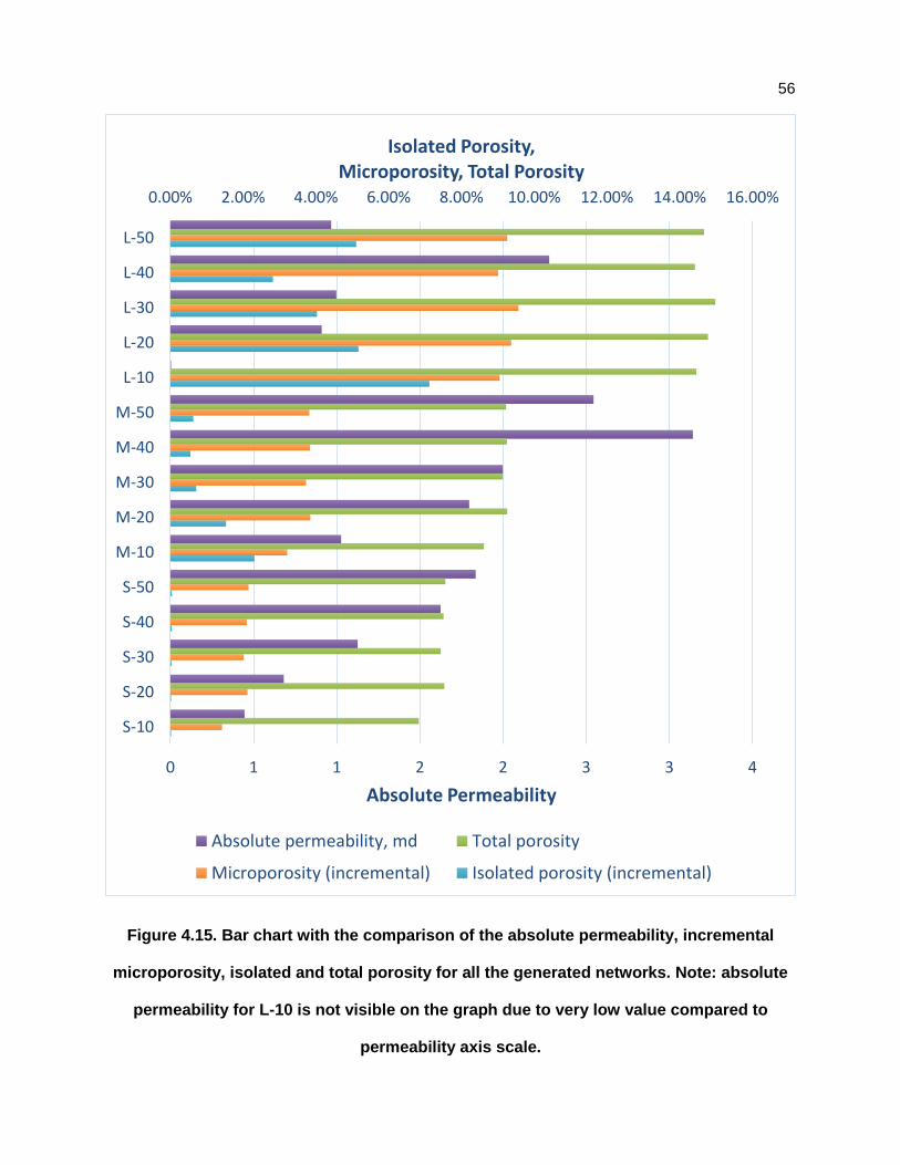
56
Figure 4.15. Bar chart with the comparison of the absolute permeability, incremental
microporosity, isolated and total porosity for all the generated networks. Note: absolute
permeability for L-10 is not visible on the graph due to very low value compared to
permeability axis scale.
0.00% 2.00% 4.00% 6.00% 8.00% 10.00% 12.00% 14.00% 16.00%
0 1 1 2 2 3 3 4
S-10
S-20
S-30
S-40
S-50
M-10
M-20
M-30
M-40
M-50
L-10
L-20
L-30
L-40
L-50
Isolated Porosity,Microporosity, Total Porosity
Absolute Permeability
Absolute permeability, md Total porosity
Microporosity (incremental) Isolated porosity (incremental)
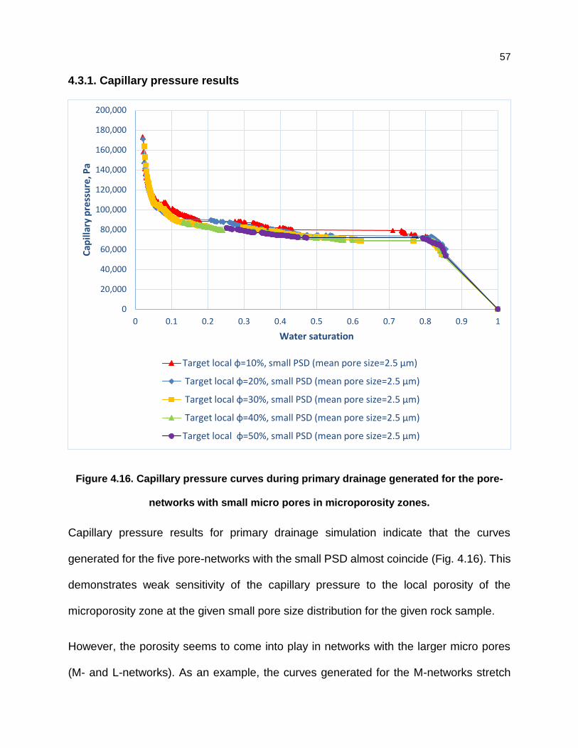
57
4.3.1. Capillary pressure results
Figure 4.16. Capillary pressure curves during primary drainage generated for the pore-
networks with small micro pores in microporosity zones.
Capillary pressure results for primary drainage simulation indicate that the curves
generated for the five pore-networks with the small PSD almost coincide (Fig. 4.16). This
demonstrates weak sensitivity of the capillary pressure to the local porosity of the
microporosity zone at the given small pore size distribution for the given rock sample.
However, the porosity seems to come into play in networks with the larger micro pores
(M- and L-networks). As an example, the curves generated for the M-networks stretch
0
20,000
40,000
60,000
80,000
100,000
120,000
140,000
160,000
180,000
200,000
0 0.1 0.2 0.3 0.4 0.5 0.6 0.7 0.8 0.9 1
Cap
illar
y p
ress
ure
, Pa
Water saturation
Target local ф=10%, small PSD (mean pore size=2.5 µm)
Target local ф=20%, small PSD (mean pore size=2.5 µm)
Target local ф=30%, small PSD (mean pore size=2.5 µm)
Target local ф=40%, small PSD (mean pore size=2.5 µm)
Target local ф=50%, small PSD (mean pore size=2.5 µm)
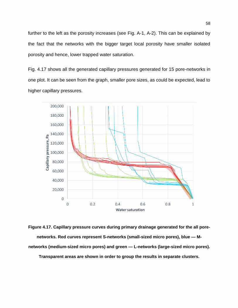
58
further to the left as the porosity increases (see Fig. A-1, A-2). This can be explained by
the fact that the networks with the bigger target local porosity have smaller isolated
porosity and hence, lower trapped water saturation.
Fig. 4.17 shows all the generated capillary pressures generated for 15 pore-networks in
one plot. It can be seen from the graph, smaller pore sizes, as could be expected, lead to
higher capillary pressures.
Figure 4.17. Capillary pressure curves during primary drainage generated for the all pore-
networks. Red curves represent S-networks (small-sized micro pores), blue — M-
networks (medium-sized micro pores) and green — L-networks (large-sized micro pores).
Transparent areas are shown in order to group the results in separate clusters.

59
4.3.2. Relative permeability results
The relative permeability results for S-networks during primary drainage can be seen on
Fig. 4.18. Similarly to capillary pressure results, all 5 curves overlap indicating weak
sensitivity to the local porosity within microporosity zones. However, for the bigger pore
sizes (M- and L-networks) with the different local porosities the curves become more
spreaded although a clear trend with regard to local porosity cannot be established
(Appendix B-1, B-2).
The big impact of pore size distribution on the results can be observed again when all the
15 cases are plotted in one figure (Fig. 4.19). General trend, as expected, is that
increasing pore sizes, due to having smaller entry capillary pressures, speed up oil
invasion and oil reaching to outlet — that is why oil relative permeability shoots up to high
values in L-networks much earlier than that occurs in S- and M-networks (Fig. 4.20). At
the same time, in the networks with the larger pores water relative permeability drops
much faster than that happens in the other two groups of networks (S- and M-) because
of oil already invading the majority of the pores right at the beginning of the drainage.
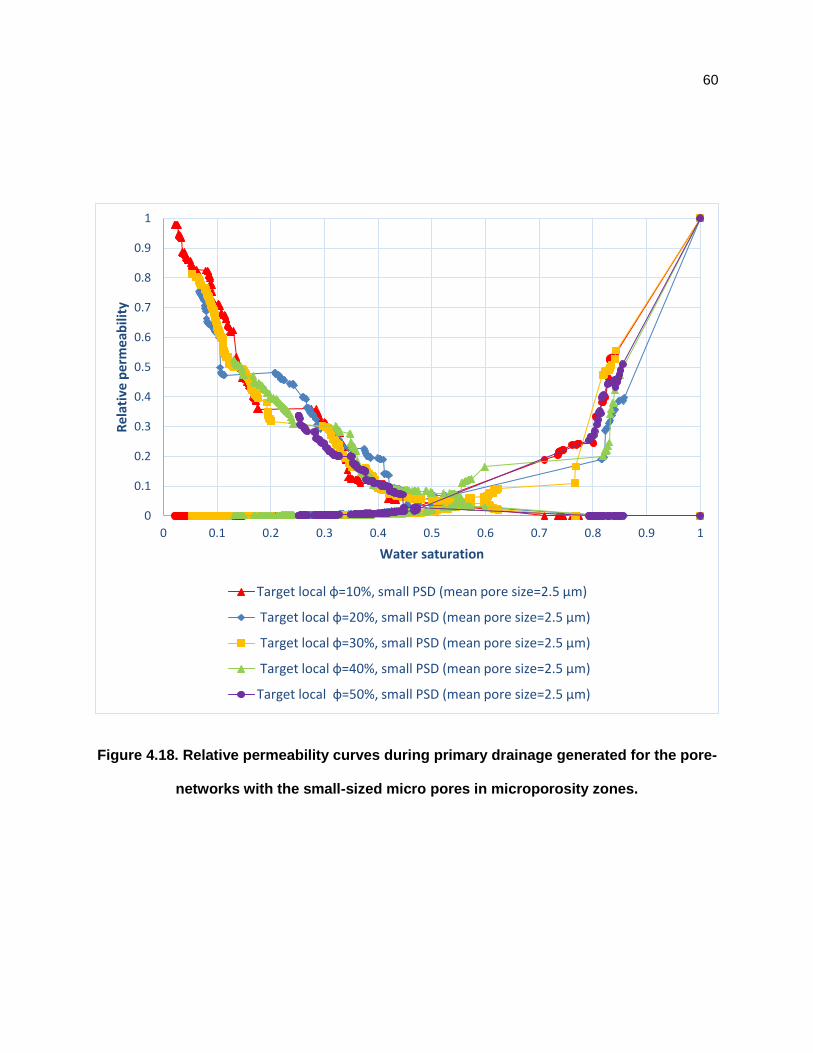
60
Figure 4.18. Relative permeability curves during primary drainage generated for the pore-
networks with the small-sized micro pores in microporosity zones.
0
0.1
0.2
0.3
0.4
0.5
0.6
0.7
0.8
0.9
1
0 0.1 0.2 0.3 0.4 0.5 0.6 0.7 0.8 0.9 1
Re
lati
ve p
erm
eab
ility
Water saturation
Target local ф=10%, small PSD (mean pore size=2.5 µm)
Target local ф=20%, small PSD (mean pore size=2.5 µm)
Target local ф=30%, small PSD (mean pore size=2.5 µm)
Target local ф=40%, small PSD (mean pore size=2.5 µm)
Target local ф=50%, small PSD (mean pore size=2.5 µm)
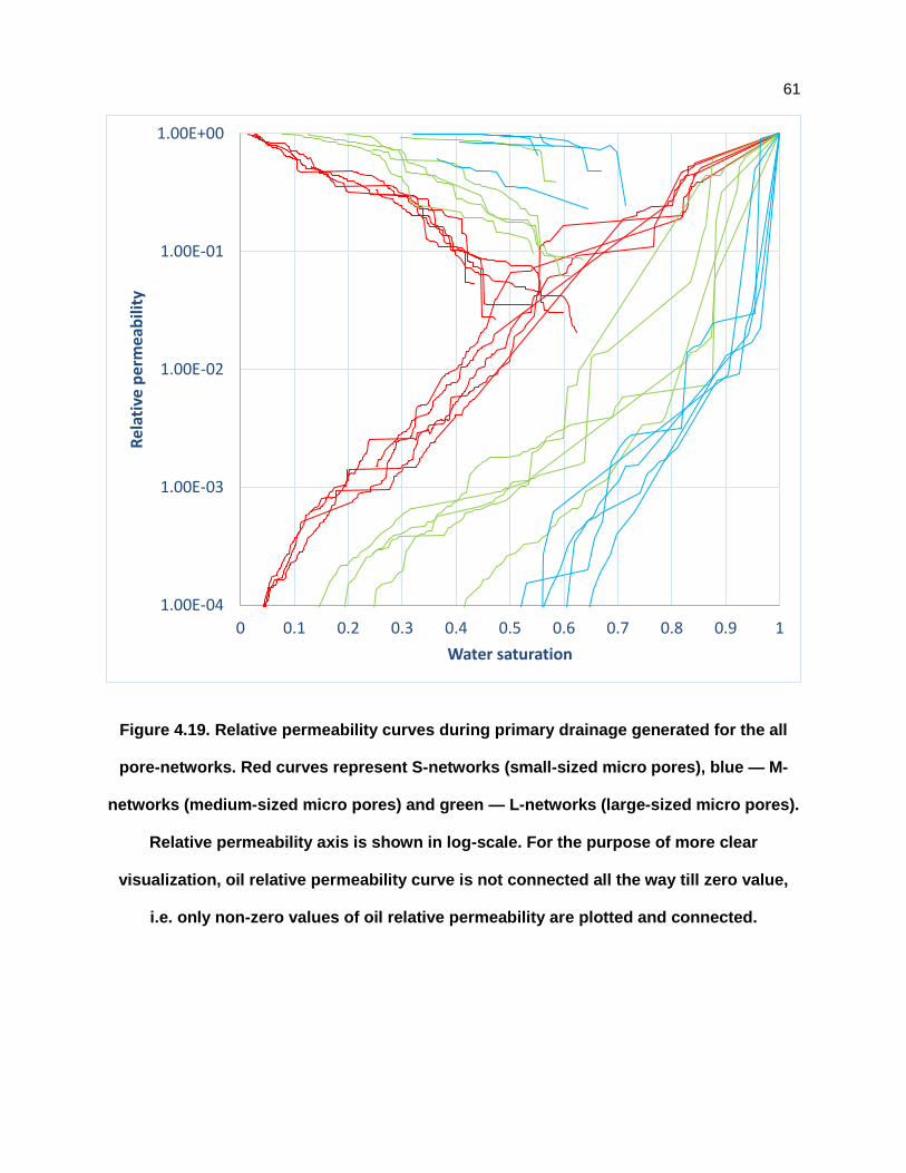
61
Figure 4.19. Relative permeability curves during primary drainage generated for the all
pore-networks. Red curves represent S-networks (small-sized micro pores), blue — M-
networks (medium-sized micro pores) and green — L-networks (large-sized micro pores).
Relative permeability axis is shown in log-scale. For the purpose of more clear
visualization, oil relative permeability curve is not connected all the way till zero value,
i.e. only non-zero values of oil relative permeability are plotted and connected.
1.00E-04
1.00E-03
1.00E-02
1.00E-01
1.00E+00
0 0.1 0.2 0.3 0.4 0.5 0.6 0.7 0.8 0.9 1
Rel
ativ
e p
erm
eab
ility
Water saturation
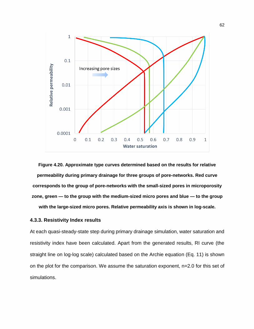
62
Figure 4.20. Approximate type curves determined based on the results for relative
permeability during primary drainage for three groups of pore-networks. Red curve
corresponds to the group of pore-networks with the small-sized pores in microporosity
zone, green — to the group with the medium-sized micro pores and blue — to the group
with the large-sized micro pores. Relative permeability axis is shown in log-scale.
4.3.3. Resistivity Index results
At each quasi-steady-state step during primary drainage simulation, water saturation and
resistivity index have been calculated. Apart from the generated results, RI curve (the
straight line on log-log scale) calculated based on the Archie equation (Eq. 11) is shown
on the plot for the comparison. We assume the saturation exponent, n=2.0 for this set of
simulations.
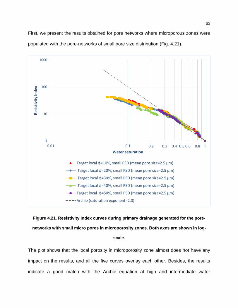
63
First, we present the results obtained for pore networks where microporous zones were
populated with the pore-networks of small pore size distribution (Fig. 4.21).
Figure 4.21. Resistivity Index curves during primary drainage generated for the pore-
networks with small micro pores in microporosity zones. Both axes are shown in log-
scale.
The plot shows that the local porosity in microporosity zone almost does not have any
impact on the results, and all the five curves overlay each other. Besides, the results
indicate a good match with the Archie equation at high and intermediate water
0.2 0.3 0.4 0.5 0.6 0.8
1
10
100
1000
0.01 0.1 1
Re
sist
ivit
y In
dex
Water saturation
Target local ф=10%, small PSD (mean pore size=2.5 µm)
Target local ф=20%, small PSD (mean pore size=2.5 µm)
Target local ф=30%, small PSD (mean pore size=2.5 µm)
Target local ф=40%, small PSD (mean pore size=2.5 µm)
Target local ф=50%, small PSD (mean pore size=2.5 µm)
Archie (saturation exponent=2.0)
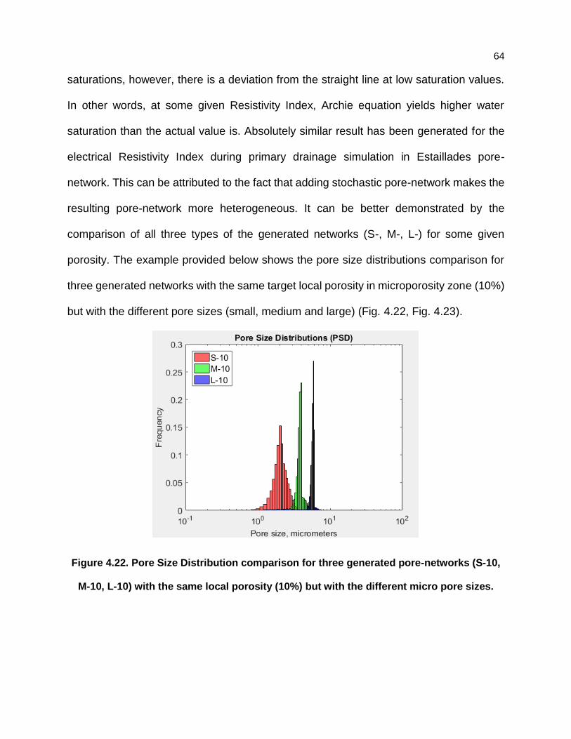
64
saturations, however, there is a deviation from the straight line at low saturation values.
In other words, at some given Resistivity Index, Archie equation yields higher water
saturation than the actual value is. Absolutely similar result has been generated for the
electrical Resistivity Index during primary drainage simulation in Estaillades pore-
network. This can be attributed to the fact that adding stochastic pore-network makes the
resulting pore-network more heterogeneous. It can be better demonstrated by the
comparison of all three types of the generated networks (S-, M-, L-) for some given
porosity. The example provided below shows the pore size distributions comparison for
three generated networks with the same target local porosity in microporosity zone (10%)
but with the different pore sizes (small, medium and large) (Fig. 4.22, Fig. 4.23).
Figure 4.22. Pore Size Distribution comparison for three generated pore-networks (S-10,
M-10, L-10) with the same local porosity (10%) but with the different micro pore sizes.
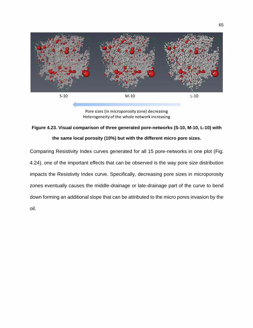
65
Figure 4.23. Visual comparison of three generated pore-networks (S-10, M-10, L-10) with
the same local porosity (10%) but with the different micro pore sizes.
Comparing Resistivity Index curves generated for all 15 pore-networks in one plot (Fig.
4.24), one of the important effects that can be observed is the way pore size distribution
impacts the Resistivity Index curve. Specifically, decreasing pore sizes in microporosity
zones eventually causes the middle-drainage or late-drainage part of the curve to bend
down forming an additional slope that can be attributed to the micro pores invasion by the
oil.
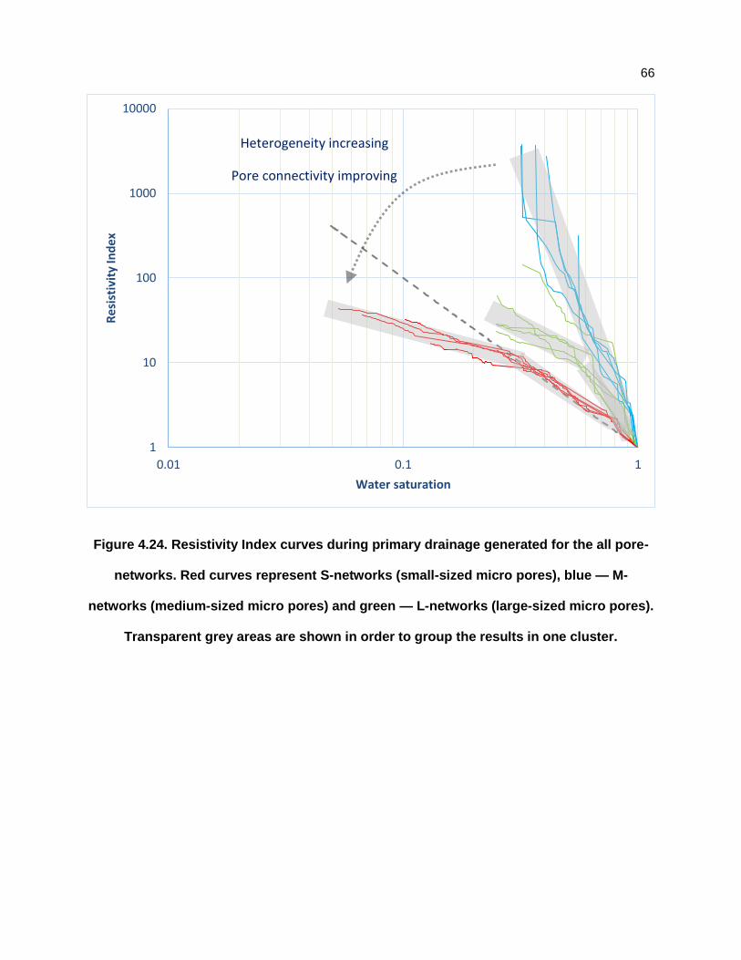
66
Figure 4.24. Resistivity Index curves during primary drainage generated for the all pore-
networks. Red curves represent S-networks (small-sized micro pores), blue — M-
networks (medium-sized micro pores) and green — L-networks (large-sized micro pores).
Transparent grey areas are shown in order to group the results in one cluster.
1
10
100
1000
10000
0.01 0.1 1
Re
sist
ivit
y In
dex
Water saturation
Heterogeneity increasing
Pore connectivity improving
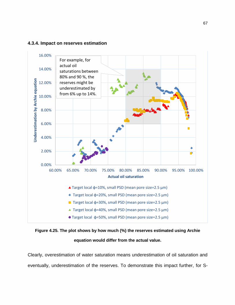
67
4.3.4. Impact on reserves estimation
Figure 4.25. The plot shows by how much (%) the reserves estimated using Archie
equation would differ from the actual value.
Clearly, overestimation of water saturation means underestimation of oil saturation and
eventually, underestimation of the reserves. To demonstrate this impact further, for S-
0.00%
2.00%
4.00%
6.00%
8.00%
10.00%
12.00%
14.00%
16.00%
60.00% 65.00% 70.00% 75.00% 80.00% 85.00% 90.00% 95.00% 100.00%
Un
de
rest
imat
ion
by
Arc
hie
eq
uat
ion
Actual oil saturation
Target local ф=10%, small PSD (mean pore size=2.5 µm)
Target local ф=20%, small PSD (mean pore size=2.5 µm)
Target local ф=30%, small PSD (mean pore size=2.5 µm)
Target local ф=40%, small PSD (mean pore size=2.5 µm)
Target local ф=50%, small PSD (mean pore size=2.5 µm)
For example, for actual oil saturations between 80% and 90 %, the reserves might be underestimated by from 6% up to 14%.
68
group of networks, the differences are calculated between actual and estimated oil
saturations ( Actual So- Estimated So
Actual So ×100% ) and are shown in the Fig. 4.25.
Chapter 5. Discussion & conclusion
We improved the model of Zolfaghari and Piri (2015a) to calculate the electrical properties
of porous media during drainage and imbibition flow cycles. The model investigates the
impact of microporosity on the electrical properties of porous media where the wetting
phase resides at corners. To do so, we built angular pore networks on 2D lattices and
added microporosity regions to generate bimodal pore networks. Five different groups of
pore networks were generated to study the impact of variable arrangements of the
microporosity regions. The results show that the intraparticle microporosity can
significantly lower electrical resistance by providing a shorter pathway for the electrical
current. Pro-vertical micro-networks (parallel microporosity) do not affect electrical
properties as much since they do not alter the shortest path of the flow. In-series
microporosity has a much more significant effect on the electrical properties. Electrical
tortuosity has a strong positive correlation with the electrical resistance: higher tortuosity
means higher electrical resistance. Using representative 3D pore networks, we also
calculated the Resistivity Index (RI) of Estaillades limestone and Berea sandstone
samples. We demonstrated the non-Archie behavior of RI at low water saturation in a
more heterogeneous sample, i.e., Estaillades limestone. The fact of having a very wide
range of pore sizes and the pore volume distributed irregularly throughout the network is
the underlying cause of sudden changes in water saturation of Estaillades networks which
can be observed on the RI curve with drastic changes of the original slope. Since the
69
majority of larger pores are surrounded by small pores, oil invades larger pores
instantaneously once the neighboring smaller pores are invaded during drainage.
Therefore, a large volume of water is displaced in a single displacement event causing
an abrupt change in the water saturation. Further work needs to be done to incorporate
Archie parameters such as saturation exponent and cementation factor in the Pore
Network Models.
We also simulated microporosity regions of a reservoir carbonate sample using our
developed Pore-Scale Network Model. We specifically studied the effect of different local
porosities and pore size distributions of microporosity zones by generating stochastic
pore networks within the Euclidean space of the microporosity clusters.
Results indicate that pore size distribution within the microporosity zone has a much
stronger impact on the results (i.e., capillary pressure, relative permeabilities and
resistivity index curve) rather than local porosity. However, as the micropore sizes are
increasing, results vary in a wide range and show more sensitivity to the local porosity
values. Generally, the pore networks generated with the chosen small Pore Size
Distribution (PSD) of the micropores seems to better replicate the pore space in
microporosity zone. Resistivity Index curve for this group of networks shows non-Archie
behavior with two slopes which is consistent with the simulated result of Estaillades
limestone.
70
References
Aghaei, A. & Piri, M. (2015). Direct pore-to-core up-scaling of displacement processes: Dynamic
pore network modeling and experimentation. Journal of hydrology, 522, 488-509.
Ahmed, T. (2010). Reservoir engineering Handbook Gulf Professional Publishing.
Ahr, W. M. (2011). Geology of carbonate reservoirs: the identification, description and
characterization of hydrocarbon reservoirs in carbonate rocks. John Wiley & Sons.
Ahrenholz, B., Tölke, J., Lehmann, P., Peters, A., Kaestner, A., Krafczyk, M., & Durner, W.
(2008). Prediction of capillary hysteresis in a porous material using lattice-Boltzmann methods
and comparison to experimental data and a morphological pore network model. Advances in
Water Resources, 31(9), 1151-1173.
Akbar, M., Vissapragada, B., Alghamdi, A. H., Allen, D., Herron, M., Carnegie, A., Dutta, D.,
Olesen, J.R., Chourasiya, R.D., Logan, D. & Stief, D. (2000). A snapshot of carbonate
reservoir evaluation. Oilfield Review, 12(4), 20-21.
Al-Marzouqi, M. I., Budebes, S., Sultan, E., Bush, I., Griffiths, R., Gzara, K. B., ... & Montaron,
B. (2010). Resolving carbonate complexity. Oilfield review, 22(2), 40-55.
Archie, G. E. (1942). The electrical resistivity log as an aid in determining some reservoir
characteristics. Transactions of the AIME, 146(01), 54-62.
Bauer, D., Youssef, S., Fleury, M., Bekri, S., Rosenberg, E., & Vizika, O. (2012). Improving the
estimations of petrophysical transport behavior of carbonate rocks using a dual pore network
approach combined with computed microtomography. Transport in porous media, 94(2), 505-
524.
Bauer, D., Youssef, S., Han, M., Bekri, S., Rosenberg, E., Fleury, M., & Vizika, O. (2011). From
computed microtomography images to resistivity index calculations of heterogeneous
carbonates using a dual-porosity pore-network approach: Influence of percolation on the
electrical transport properties. Physical review E, 84(1), 011133.
Bear, J., Tsang, C. F., & De Marsily, G. (2012). Flow and contaminant transport in fractured rock.
Academic Press.
Bekri, S., Laroche, C., & Vizika, O. (2005, August). Pore network models to calculate transport
and electrical properties of single or dual-porosity rocks. In SCA (Vol. 35, p. 2005).
Blunt, M. J. (2017). Multiphase flow in permeable media: A pore-scale perspective. Cambridge
University Press.
Blunt, M. J., Bijeljic, B., Dong, H., Gharbi, O., Iglauer, S., Mostaghimi, P., Paluszny, A. &
Pentland, C. (2013). Pore-scale imaging and modelling. Advances in Water Resources, 51,
197-216.
Blunt, M. J., Jackson, M. D., Piri, M., & Valvatne, P. H. (2002). Detailed physics, predictive
capabilities and macroscopic consequences for pore-network models of multiphase flow.
Advances in Water Resources, 25(8-12), 1069-1089.
Boek, E. S., & Venturoli, M. (2010). Lattice-Boltzmann studies of fluid flow in porous media with
realistic rock geometries. Computers & Mathematics with Applications, 59(7), 2305-2314.
Boyd, A., Darling, H., Tabanou, J., Davis, B., Lyon, B., Flaum, C., Klein J., Sneider R., Sibbit A.
& Singer, J. (1995). The lowdown on low-resistivity pay. Oilfield Review, 7(3), 4-18.
Bultreys, T., De Boever, W., & Cnudde, V. (2016). Imaging and image-based fluid transport
modeling at the pore scale in geological materials: A practical introduction to the current state-
of-the-art. Earth-Science Reviews, 155, 93-128.
71
Bultreys, T., Lin, Q., Gao, Y., Raeini, A. Q., AlRatrout, A., Bijeljic, B., & Blunt, M. J. (2018).
Validation of model predictions of pore-scale fluid distributions during two-phase flow.
Physical Review E, 97(5), 053104.
Bultreys, T., Van Hoorebeke, L., & Cnudde, V. (2015). Multi-scale, micro-computed tomography-
based pore network models to simulate drainage in heterogeneous rocks. Advances in Water
Resources, 78, 36-49.
Cantrell, D. L., & Hagerty, R. M. (1999). Microporosity in arab formation carbonates, Saudi
Arabia. GeoArabia, 4(2), 129-154.
Chin, J. (2002). Lattice Boltzmann simulation of the flow of binary immiscible fluids with different
viscosities using the Shan-Chen microscopic interaction model. Philosophical Transactions of
the Royal Society of London. Series A: Mathematical, Physical and Engineering Sciences,
360(1792), 547-558.
Choquette, P. W., & Pray, L. C. (1970). Geologic nomenclature and classification of porosity in
sedimentary carbonates. AAPG bulletin, 54(2), 207-250.
Clennell, M. B. (1997). Tortuosity: a guide through the maze. Geological Society, London, Special
Publications, 122(1), 299-344.
Coates, G. R., Xiao, L., & Prammer, M. G. (1999). NMR logging: principles and applications (Vol.
234). Houston: Haliburton Energy Services.
Doveton, J. H. (2001). Development of an Archie Equation Model for Log Analysis of
Pennsylvanian Oomoldic Zones in Kansas. KGS Open File Report.
Ehrenberg, S. N., & Walderhaug, O. (2015). Preferential calcite cementation of macropores in
microporous limestones. Journal of Sedimentary Research, 85(7), 780-793.
Fatt, I. (1956). The network model of porous media.
Fleury, M., Efnik, M., & Kalam, M. Z. (2004, October). Evaluation of water saturation from
resistivity in a carbonate field. From laboratory to logs. In Proceedings of International
Symposium of the Society of Core Analysts, Abu Dhabi, UAE (pp. 5-9).
Gundogar, A. S., Ross, C. M., Akin, S., & Kovscek, A. R. (2016). Multiscale pore structure
characterization of Middle East carbonates. Journal of Petroleum Science and Engineering,
146, 570-583.
Hakimov, N., Zolfaghari, A., Kalantari-Dahaghi, A., Negahban, S., & Gunter, G. (2018,
November). Pore-Scale Network Modeling of Petrophysical Properties in Samples with Wide
Pore Size Distributions. In Abu Dhabi International Petroleum Exhibition & Conference.
Society of Petroleum Engineers.
Hamada, G. M., Almajed, A. A., Okasha, T. M., & Algathe, A. A. (2013). Uncertainty analysis of
Archie’s parameters determination techniques in carbonate reservoirs. Journal of Petroleum
Exploration and Production Technology, 3(1), 1-10.
Hassan, A., Chandra, V., Yutkin, M. P., Patzek, T. W., & Espinoza, D. N. (2019). Imaging and
Characterization of Microporous Carbonates Using Confocal and Electron Microscopy of
Epoxy Pore Casts. SPE Journal.
Icardi, M., Boccardo, G., Marchisio, D. L., Tosco, T., & Sethi, R. (2014). Pore-scale simulation of
fluid flow and solute dispersion in three-dimensional porous media. Physical review E, 90(1),
013032.
Jiang, Z., Van Dijke, M. I. J., Sorbie, K. S., & Couples, G. D. (2013). Representation of multiscale
heterogeneity via multiscale pore networks. Water resources research, 49(9), 5437-5449.
Jiang, Z., Van Dijke, M. I. J., Wu, K., Couples, G. D., Sorbie, K. S., & Ma, J. (2012). Stochastic
pore network generation from 3D rock images. Transport in porous media, 94(2), 571-593.
72
Joekar-Niasar, V., Hassanizadeh, S. M., & Dahle, H. K. (2010). Non-equilibrium effects in
capillarity and interfacial area in two-phase flow: dynamic pore-network modelling. Journal
of Fluid Mechanics, 655, 38-71.
Karpyn, Z. T., & Piri, M. (2007). Prediction of fluid occupancy in fractures using network
modeling and x-ray microtomography. I: Data conditioning and model description. Physical
Review E, 76(1), 016315.
Leon y Leon, C. A. L. (1998). New perspectives in mercury porosimetry. Advances in colloid and
interface science, 76, 341-372.
Mayer, R. P., & Stowe, R. A. (1965). Mercury porosimetry—breakthrough pressure for
penetration between packed spheres. Journal of colloid Science, 20(8), 893-911.
Meakin, P., & Tartakovsky, A. M. (2009). Modeling and simulation of pore‐scale multiphase fluid
flow and reactive transport in fractured and porous media. Reviews of Geophysics, 47(3).
Mehmani, A., & Prodanović, M. (2014). The effect of microporosity on transport properties in
porous media. Advances in Water Resources, 63, 104-119.
Miao, X., Gerke, K. M., & Sizonenko, T. O. (2017). A new way to parameterize hydraulic
conductances of pore elements: A step towards creating pore-networks without pore shape
simplifications. Advances in water resources, 105, 162-172.
Mohammadmoradi, P., & Kantzas, A. (2017). Toward direct pore-scale modeling of three-phase
displacements. Advances in water resources, 110, 120-135.
Morad, D., Paganoni, M., Al Harthi, A., Morad, S., Ceriani, A., Mansurbeg, H., Al Suwaidi, A.,
Al-Aasm, I.S & Ehrenberg, S. N. (2018). Origin and evolution of microporosity in packstones
and grainstones in a Lower Cretaceous carbonate reservoir, United Arab Emirates. Geological
Society, London, Special Publications, 435(1), 47-66.
Norbisrath, J. H., Eberli, G. P., Laurich, B., Desbois, G., Weger, R. J., & Urai, J. L. (2015).
Electrical and fluid flow properties of carbonate microporosity types from multiscale digital
image analysis and mercury injection. AAPG Bulletin, 99(11), 2077-2098.
Oren, P. E., Bakke, S., & Arntzen, O. J. (1997, January). Extending predictive capabilities to
network models. In SPE Annual Technical Conference and Exhibition. Society of Petroleum
Engineers.
Pak, T., Butler, I. B., Geiger, S., van Dijke, M. I., Jiang, Z., & Surmas, R. (2016). Multiscale pore‐network representation of heterogeneous carbonate rocks. Water Resources Research, 52(7),
5433-5441.
Pan, C., Hilpert, M., & Miller, C. T. (2004). Lattice‐Boltzmann simulation of two‐phase flow in
porous media. Water Resources Research, 40(1).
Piri, M. (2003). "Pore-scale modelling of three-phase flow." PhD Disseration. Imperial College.
Piri, M., & Blunt, M. J. (2005a). Three-dimensional mixed-wet random pore-scale network
modeling of two-and three-phase flow in porous media. I. Model description. Physical Review
E, 71(2), 026301.
Piri, M., & Blunt, M. J. (2005b). Three-dimensional mixed-wet random pore-scale network
modeling of two-and three-phase flow in porous media. II. Results. Physical Review E, 71(2),
026302.
Piri, M., & Karpyn, Z. T. (2007). Prediction of fluid occupancy in fractures using network
modeling and X-ray microtomography. II: Results. Physical Review E, 76(1), 016316.
Princen, H. M. (1969a). Capillary phenomena in assemblies of parallel cylinders: I. Capillary rise
between two cylinders. Journal of Colloid and Interface Science, 30(1), 69-75.
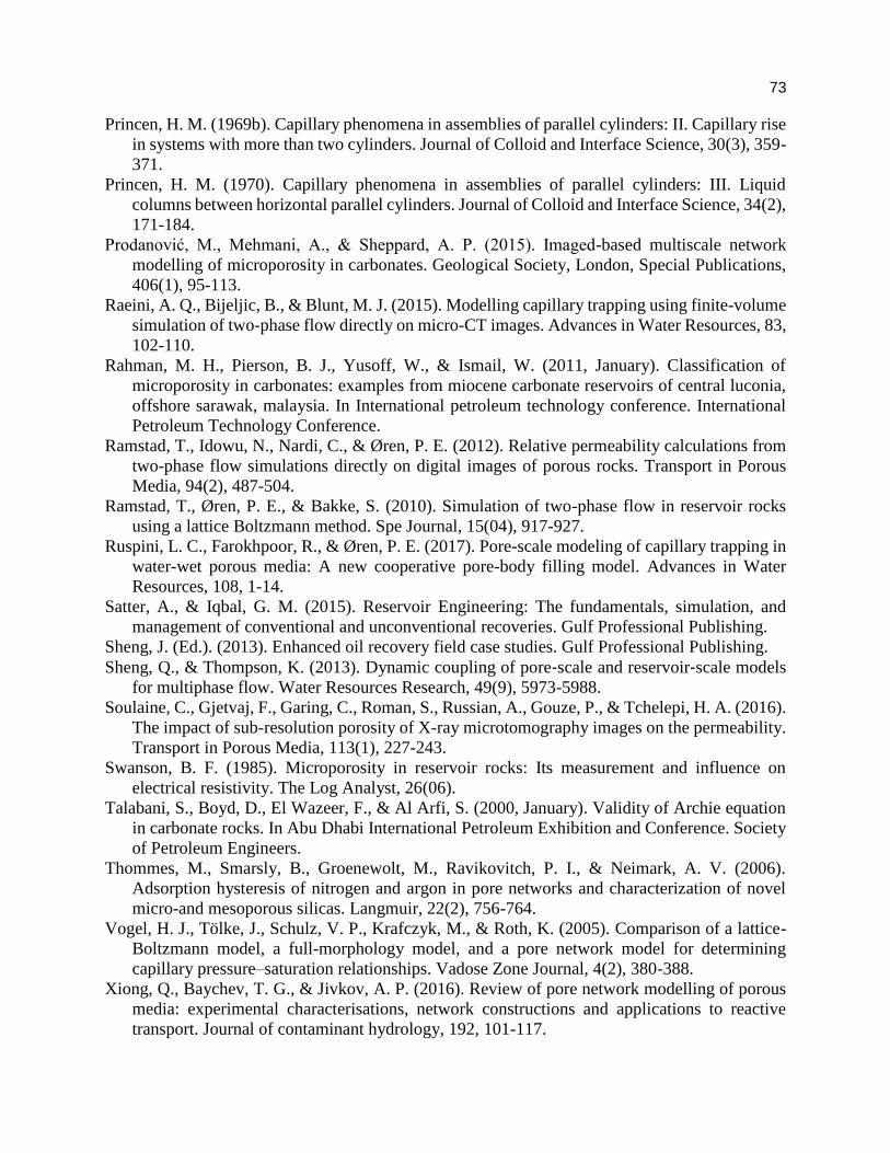
73
Princen, H. M. (1969b). Capillary phenomena in assemblies of parallel cylinders: II. Capillary rise
in systems with more than two cylinders. Journal of Colloid and Interface Science, 30(3), 359-
371.
Princen, H. M. (1970). Capillary phenomena in assemblies of parallel cylinders: III. Liquid
columns between horizontal parallel cylinders. Journal of Colloid and Interface Science, 34(2),
171-184.
Prodanović, M., Mehmani, A., & Sheppard, A. P. (2015). Imaged-based multiscale network
modelling of microporosity in carbonates. Geological Society, London, Special Publications,
406(1), 95-113.
Raeini, A. Q., Bijeljic, B., & Blunt, M. J. (2015). Modelling capillary trapping using finite-volume
simulation of two-phase flow directly on micro-CT images. Advances in Water Resources, 83,
102-110.
Rahman, M. H., Pierson, B. J., Yusoff, W., & Ismail, W. (2011, January). Classification of
microporosity in carbonates: examples from miocene carbonate reservoirs of central luconia,
offshore sarawak, malaysia. In International petroleum technology conference. International
Petroleum Technology Conference.
Ramstad, T., Idowu, N., Nardi, C., & Øren, P. E. (2012). Relative permeability calculations from
two-phase flow simulations directly on digital images of porous rocks. Transport in Porous
Media, 94(2), 487-504.
Ramstad, T., Øren, P. E., & Bakke, S. (2010). Simulation of two-phase flow in reservoir rocks
using a lattice Boltzmann method. Spe Journal, 15(04), 917-927.
Ruspini, L. C., Farokhpoor, R., & Øren, P. E. (2017). Pore-scale modeling of capillary trapping in
water-wet porous media: A new cooperative pore-body filling model. Advances in Water
Resources, 108, 1-14.
Satter, A., & Iqbal, G. M. (2015). Reservoir Engineering: The fundamentals, simulation, and
management of conventional and unconventional recoveries. Gulf Professional Publishing.
Sheng, J. (Ed.). (2013). Enhanced oil recovery field case studies. Gulf Professional Publishing.
Sheng, Q., & Thompson, K. (2013). Dynamic coupling of pore‐scale and reservoir‐scale models
for multiphase flow. Water Resources Research, 49(9), 5973-5988.
Soulaine, C., Gjetvaj, F., Garing, C., Roman, S., Russian, A., Gouze, P., & Tchelepi, H. A. (2016).
The impact of sub-resolution porosity of X-ray microtomography images on the permeability.
Transport in Porous Media, 113(1), 227-243.
Swanson, B. F. (1985). Microporosity in reservoir rocks: Its measurement and influence on
electrical resistivity. The Log Analyst, 26(06).
Talabani, S., Boyd, D., El Wazeer, F., & Al Arfi, S. (2000, January). Validity of Archie equation
in carbonate rocks. In Abu Dhabi International Petroleum Exhibition and Conference. Society
of Petroleum Engineers.
Thommes, M., Smarsly, B., Groenewolt, M., Ravikovitch, P. I., & Neimark, A. V. (2006).
Adsorption hysteresis of nitrogen and argon in pore networks and characterization of novel
micro-and mesoporous silicas. Langmuir, 22(2), 756-764.
Vogel, H. J., Tölke, J., Schulz, V. P., Krafczyk, M., & Roth, K. (2005). Comparison of a lattice-
Boltzmann model, a full-morphology model, and a pore network model for determining
capillary pressure–saturation relationships. Vadose Zone Journal, 4(2), 380-388.
Xiong, Q., Baychev, T. G., & Jivkov, A. P. (2016). Review of pore network modelling of porous
media: experimental characterisations, network constructions and applications to reactive
transport. Journal of contaminant hydrology, 192, 101-117.
74
Yang, J., Bondino, I., Regaieg, M., & Moncorgé, A. (2017). Pore to pore validation of pore
network modelling against micromodel experiment results. Computational Geosciences, 21(5-
6), 849-862.
Zolfaghari, A. (2014). “Pore-scale Network Modeling of Two-and Three-phase Flow Based on
Thermodynamically Consistent Threshold Capillary Pressures” PhD Disseration. University
of Wyoming.
Zolfaghari, A., & Piri, M. (2017a). Pore-scale network modeling of three-phase flow based on
thermodynamically consistent threshold capillary pressures. I. Cusp formation and collapse.
Transport in porous media, 116(3), 1093-1137.
Zolfaghari, A., & Piri, M. (2017b). Pore-scale network modeling of three-phase flow based on
thermodynamically consistent threshold capillary pressures. II. Results. Transport in Porous
Media, 116(3), 1139-1165.
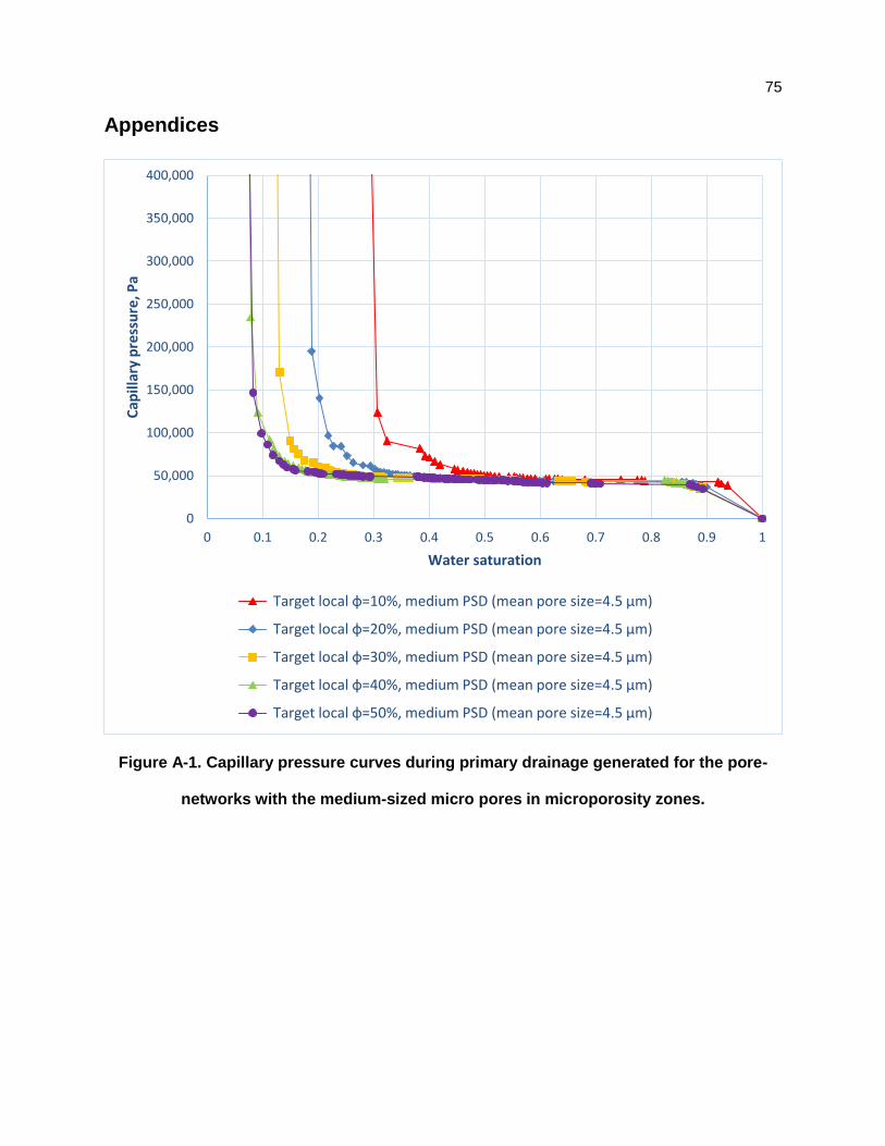
75
Appendices
Figure A-1. Capillary pressure curves during primary drainage generated for the pore-
networks with the medium-sized micro pores in microporosity zones.
0
50,000
100,000
150,000
200,000
250,000
300,000
350,000
400,000
0 0.1 0.2 0.3 0.4 0.5 0.6 0.7 0.8 0.9 1
Cap
illar
y p
ress
ure
, Pa
Water saturation
Target local ф=10%, medium PSD (mean pore size=4.5 µm)
Target local ф=20%, medium PSD (mean pore size=4.5 µm)
Target local ф=30%, medium PSD (mean pore size=4.5 µm)
Target local ф=40%, medium PSD (mean pore size=4.5 µm)
Target local ф=50%, medium PSD (mean pore size=4.5 µm)
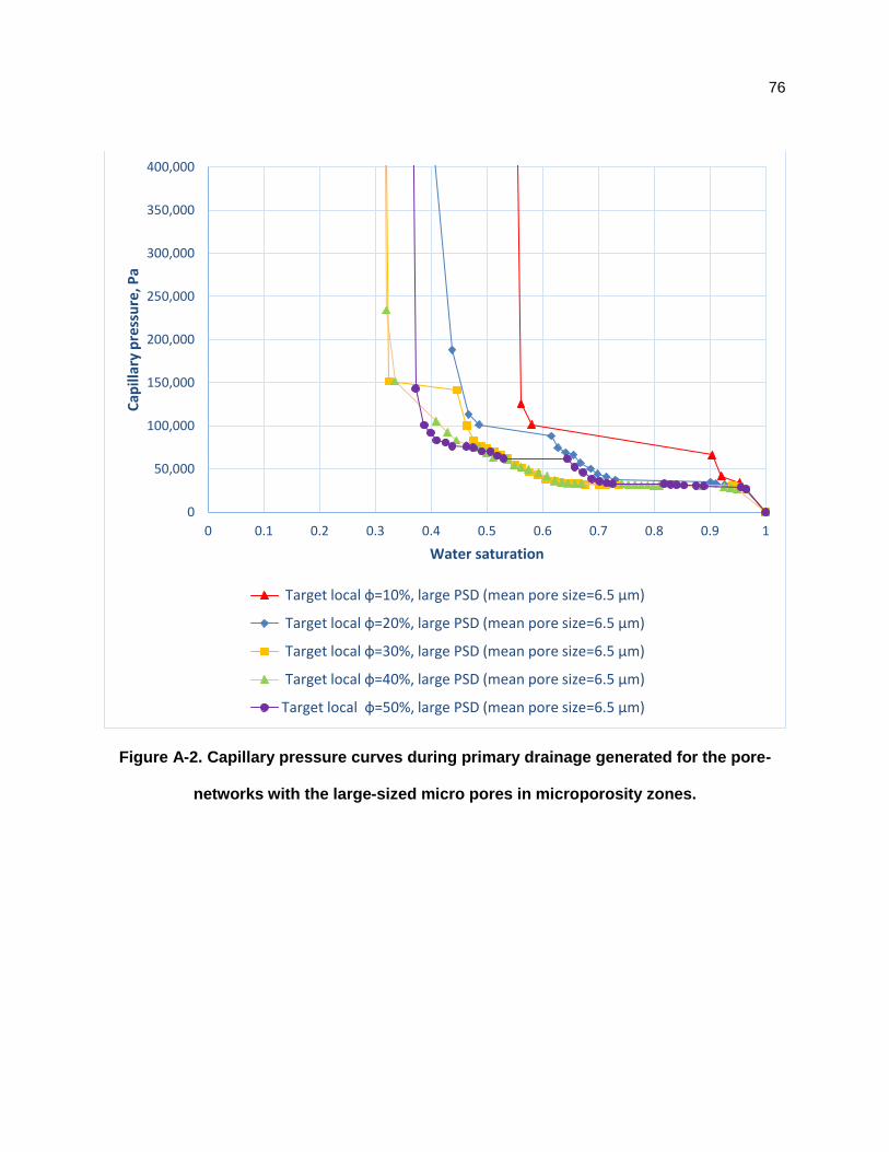
76
Figure A-2. Capillary pressure curves during primary drainage generated for the pore-
networks with the large-sized micro pores in microporosity zones.
0
50,000
100,000
150,000
200,000
250,000
300,000
350,000
400,000
0 0.1 0.2 0.3 0.4 0.5 0.6 0.7 0.8 0.9 1
Cap
illar
y p
ress
ure
, Pa
Water saturation
Target local ф=10%, large PSD (mean pore size=6.5 µm)
Target local ф=20%, large PSD (mean pore size=6.5 µm)
Target local ф=30%, large PSD (mean pore size=6.5 µm)
Target local ф=40%, large PSD (mean pore size=6.5 µm)
Target local ф=50%, large PSD (mean pore size=6.5 µm)
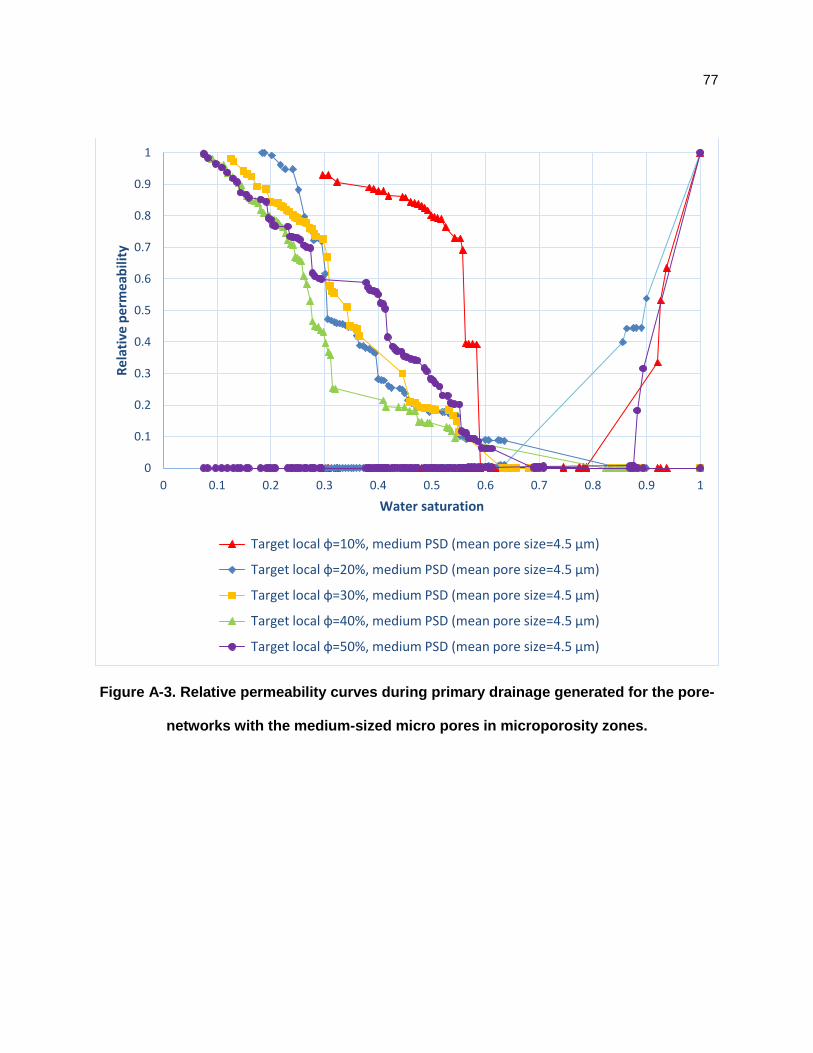
77
Figure A-3. Relative permeability curves during primary drainage generated for the pore-
networks with the medium-sized micro pores in microporosity zones.
0
0.1
0.2
0.3
0.4
0.5
0.6
0.7
0.8
0.9
1
0 0.1 0.2 0.3 0.4 0.5 0.6 0.7 0.8 0.9 1
Re
lati
ve p
erm
eab
ility
Water saturation
Target local ф=10%, medium PSD (mean pore size=4.5 µm)
Target local ф=20%, medium PSD (mean pore size=4.5 µm)
Target local ф=30%, medium PSD (mean pore size=4.5 µm)
Target local ф=40%, medium PSD (mean pore size=4.5 µm)
Target local ф=50%, medium PSD (mean pore size=4.5 µm)
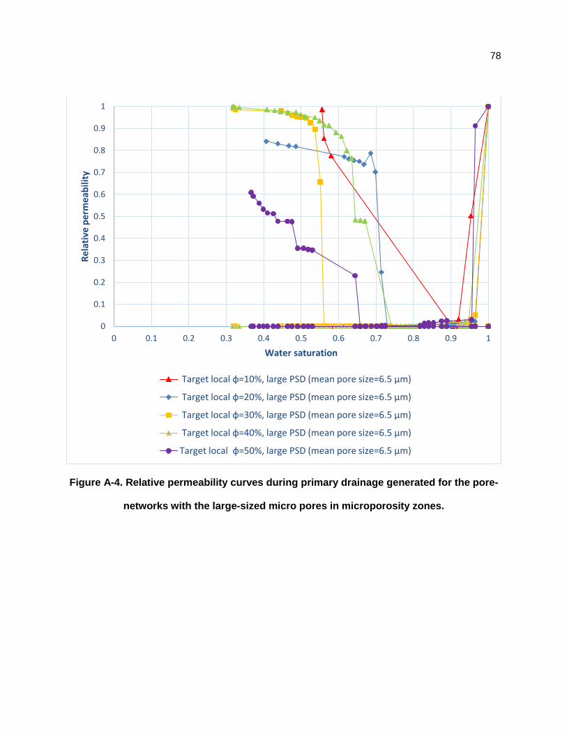
78
Figure A-4. Relative permeability curves during primary drainage generated for the pore-
networks with the large-sized micro pores in microporosity zones.
0
0.1
0.2
0.3
0.4
0.5
0.6
0.7
0.8
0.9
1
0 0.1 0.2 0.3 0.4 0.5 0.6 0.7 0.8 0.9 1
Re
lati
ve p
erm
eab
ility
Water saturation
Target local ф=10%, large PSD (mean pore size=6.5 µm)
Target local ф=20%, large PSD (mean pore size=6.5 µm)
Target local ф=30%, large PSD (mean pore size=6.5 µm)
Target local ф=40%, large PSD (mean pore size=6.5 µm)
Target local ф=50%, large PSD (mean pore size=6.5 µm)
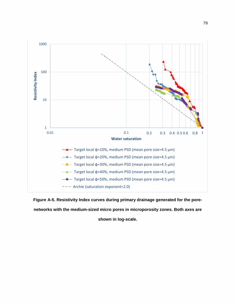
79
Figure A-5. Resistivity Index curves during primary drainage generated for the pore-
networks with the medium-sized micro pores in microporosity zones. Both axes are
shown in log-scale.
0.2 0.3 0.4 0.5 0.6 0.8
1
10
100
1000
0.01 0.1 1
Re
sist
ivit
y In
dex
Water saturation
Target local ф=10%, medium PSD (mean pore size=4.5 µm)
Target local ф=20%, medium PSD (mean pore size=4.5 µm)
Target local ф=30%, medium PSD (mean pore size=4.5 µm)
Target local ф=40%, medium PSD (mean pore size=4.5 µm)
Target local ф=50%, medium PSD (mean pore size=4.5 µm)
Archie (saturation exponent=2.0)
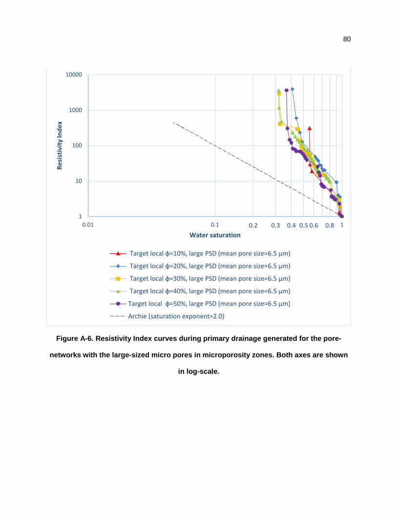
80
Figure A-6. Resistivity Index curves during primary drainage generated for the pore-
networks with the large-sized micro pores in microporosity zones. Both axes are shown
in log-scale.
0.2 0.3 0.4 0.5 0.6 0.8
1
10
100
1000
10000
0.01 0.1 1
Re
sist
ivit
y In
dex
Water saturation
Target local ф=10%, large PSD (mean pore size=6.5 µm)
Target local ф=20%, large PSD (mean pore size=6.5 µm)
Target local ф=30%, large PSD (mean pore size=6.5 µm)
Target local ф=40%, large PSD (mean pore size=6.5 µm)
Target local ф=50%, large PSD (mean pore size=6.5 µm)
Archie (saturation exponent=2.0)
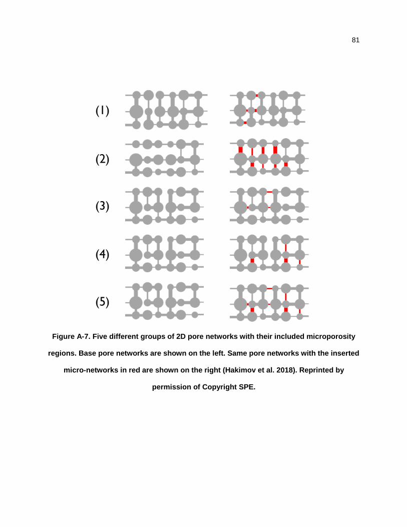
81
Figure A-7. Five different groups of 2D pore networks with their included microporosity
regions. Base pore networks are shown on the left. Same pore networks with the inserted
micro-networks in red are shown on the right (Hakimov et al. 2018). Reprinted by
permission of Copyright SPE.
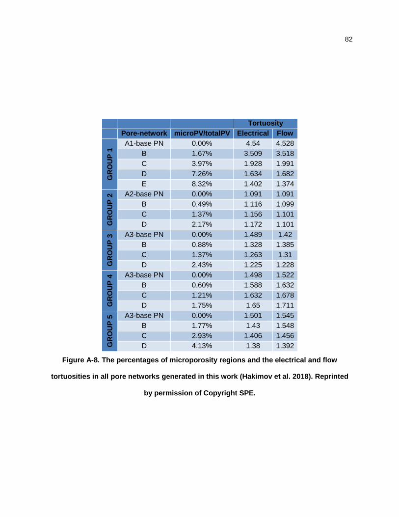
82
Tortuosity
Pore-network microPV/totalPV Electrical Flow
GR
OU
P 1
A1-base PN 0.00% 4.54 4.528
B 1.67% 3.509 3.518
C 3.97% 1.928 1.991
D 7.26% 1.634 1.682
E 8.32% 1.402 1.374
GR
OU
P 2
A2-base PN 0.00% 1.091 1.091
B 0.49% 1.116 1.099
C 1.37% 1.156 1.101
D 2.17% 1.172 1.101
GR
OU
P 3
A3-base PN 0.00% 1.489 1.42
B 0.88% 1.328 1.385
C 1.37% 1.263 1.31
D 2.43% 1.225 1.228
GR
OU
P 4
A3-base PN 0.00% 1.498 1.522
B 0.60% 1.588 1.632
C 1.21% 1.632 1.678
D 1.75% 1.65 1.711
GR
OU
P 5
A3-base PN 0.00% 1.501 1.545
B 1.77% 1.43 1.548
C 2.93% 1.406 1.456
D 4.13% 1.38 1.392
Figure A-8. The percentages of microporosity regions and the electrical and flow
tortuosities in all pore networks generated in this work (Hakimov et al. 2018). Reprinted
by permission of Copyright SPE.
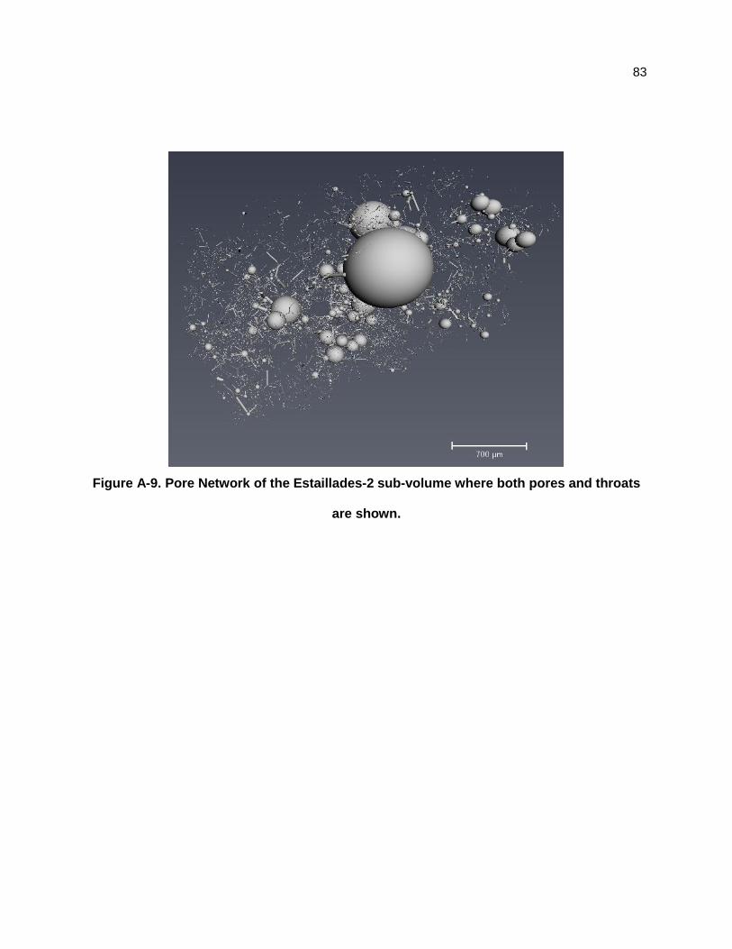
83
Figure A-9. Pore Network of the Estaillades-2 sub-volume where both pores and throats
are shown.