COUPLED PORE-TO-CONTINUUM MULTISCALE MODELING OF

DYNAMIC PARTICLE FILTRATION PROCESSES IN POROUS

MEDIA

A Dissertation

Submitted to the Graduate Faculty of the

Louisiana State University and

Agricultural and Mechanical College

in partial fulfilment of the

requirements for the degree of

Doctor of Philosophy

in

The Department of Petroleum Engineering

by

John Rayner Blears

B.S., Washington University in St. Louis, 2013

M.S., Louisiana State University, 2015

December 2019

ii

This work is dedicated to my family and friends, whose support and sacrifices throughout my life

have made this work possible.

iii

Acknowledgements

I would like to thank my committee members for their guidance and time spent during the research

for this work. I am truly grateful for the opportunities you have given me, which greatly improved

my analytical and communication skills. Specifically, I would like to thank Dr. Karsten Thompson

for the opportunity to work under his guidance as a teaching assistant, masters candidate, and

doctoral candidate. I also thank Dr. Richard Hughes and Dr. Mayank Tyagi for the opportunities

they gave me to work as a teaching assistant and for their support in the research process.

My family and friends have given me the support and encouragement needed to undertake and

complete this work. I am extremely grateful to my parents for their dedication to my wellbeing

and education. and to my siblings for their care and support. Also to Valentina Rosasco for being

with me during the during the course of this work and to all my friends who have assisted me along

the way, I thank you.

iv

Table of Contents

Acknowledgements ....................................................................................................................... iii

Abstract ........................................................................................................................................... v

Chapter 1. Introduction .................................................................................................................. 1

1.1. Overview ......................................................................................................................1

1.2. Applications ..................................................................................................................3

1.3. Experimental Observations ..........................................................................................4

1.4. Continuum-scale Modeling ..........................................................................................6

1.5. Pore-scale Modeling .....................................................................................................9

1.6. Coupled Modeling ......................................................................................................21

1.7. Objectives ...................................................................................................................24

Chapter 2. Technical Approach ................................................................................................... 25

2.1. Resources Available....................................................................................................25

2.2. Finite Difference Model .............................................................................................36

2.3. Finite Difference Model Verification and Validation .................................................40

2.4. Concurrently Coupled Model .....................................................................................54

Chapter 3. Results and Discussion ............................................................................................... 55

3.1. One-Dimensional Concurrent Coupling .....................................................................55

3.2. Three-Dimensional Concurrent Coupling.................................................................108

Conclusion ...................................................................................................................................119

Appendix. Supplementary Input Data File for Chapter 3 ........................................................... 121

References ....................................................................................................................................126

Vita .............................................................................................................................................. 137

v

Abstract

Modeling particle transport and retention in porous media is important in fields such as

hydrocarbon extraction, groundwater filtration, and membrane separation. While the continuum-

scale (>1 m) is usually of practical interest, pore-scale (1-100 μm) dynamics govern the transport

and retention of particles. Therefore, accurate modeling of continuum-scale behavior requires an

effective incorporation of pore-scale dynamics. Due to current computational limits however, the

large spatial and temporal discrepancies of these scales prohibit modeling an entire continuum-

scale system as a single pore-scale model. Even if a pore-scale model could incorporate every pore

contained in a continuum-scale system, an upscaling scheme that coupled pore- and continuum-

scale models should in principle be more efficient and achieve acceptable accuracy. In this work,

a continuum-scale model for particle transport and retention has been developed using the

concurrent coupling method. In the model, pore network models (PNMs) were embedded within

continuum-scale finite difference grid blocks. As simulations progressed the embedded PNMs

periodically provided their continuum-scale grid blocks with updated petrophysical properties.

The PNMs used a Lagrangian particle tracking method to identify particle dispersion and retention

coefficients. Any changes in permeability and porosity due to particle trapping were also

determined. Boundary conditions for the PNM simulations were prescribed by fluid velocity and

influent particle concentration information from the continuum-scale grid blocks. Coupling in this

manner allowed for a dynamic understanding of how particle induced changes at the pore-scale

impact continuum-scale behavior.

1

Chapter 1. Introduction

1.1. Overview

The study of particle transport and retention in porous media, also referred to as particle filtration

in this work, has been ongoing since the 1960s and has a wide range of applications in multiple

disciplines (Gao, 2008). Applications include water filtration (Yao et al., 1971), pathogen transport

in groundwater (McDowell-Boyer et al., 1986), hydrocarbon reservoir damage (Gao, 2007), and

transport of engineered nanoparticles (Molnar et al., 2015). For these and all other applications, a

model capable of predicting how retention of particles will impact field-scale parameters would

be highly useful. Such a model would aid in the design of effective treatments to mitigate or

enhance particle retention, depending on the nature of the application. Analytical, experimental,

and numerical methods, which have been used to understand the processes involved in particle

filtration, have provided the foundation to develop predictive continuum-scale models. To date

however, accurate models have been difficult to develop due to the complex pore geometry and

multi-scale nature of porous media.

Particle filtration models can be categorized as either continuum-scale or pore-scale models.

Continuum-scale models can be subsequently classified as trajectory analysis models or

phenomenological models. Trajectory analysis models use force balances to compute particle

trajectories and determine whether or not retention will occur (Imdakm and Sahimi, 1991). The

porous media in these models is typically represented as a collection of so-called unit collectors

which provide an attachment surface for suspended particles. While this configuration allows for

semi-analytical solutions of fluid flow and particle trajectory, the underlying simplifications of the

medium inhibit accurately modeling many systems of interest (Sahimi et al., 1990).

Alternatively, phenomenological models treat fluid and solid species concentrations as smooth

functions of time and space and are primarily based on numerical solutions to various forms of the

advection-dispersion equation (Sahimi et al., 1990). In phenomenological models, particle

retention is typically accounted for with an additional term that uses a mass transfer rate

coefficient. The mass transfer coefficients are typically empirically obtained from particle

filtration core flooding experiments (Gao, 2008). Although simpler to utilize, phenomenological

models make simplifying assumptions concerning microscopic properties of the porous medium

and do not explicitly consider the mechanisms responsible for particle retention, such as particle

size (Feng et al., 2015). These simplifications limit the practical usefulness of phenomenological

models.

In contrast, pore-scale models determine particle retention by considering the forces and transport

mechanisms acting on particles as they flow through a porous medium. Pore-scale models can be

categorized as either direct models or pore network models (PNMs). Direct models solve the

governing equations of transport and retention on direct representations of the porous medium

(Mehmani and Balhoff, 2015a). Modern computed tomography (CT) imaging techniques, such as

micro-CT scanning, have allowed for the generation of three-dimensional models of pore structure

with resolutions of a few microns (Blunt et al., 2013). Fluid flow and particle retention can then

be computed on models extracted directly from the pore-space images using numerical techniques,

such as the Lattice Boltzmann Method (LBM) or the finite element method (FEM). The high

2

resolution and accuracy of modern direct pore-scale models however, is associated with large

computational requirements. For systems containing tens or hundreds of interconnected pores,

analytical complexities are compounded, causing the computational requirements needed to obtain

solutions to become intractable (Tartakovsky et al., 2007).

In comparison, PNMs represent porous media as simplified networks of pores connected by

throats. Both pores and throats are given simple geometries, with the most commonly used

geometries being spheres for pores and cylinders for throats (Xiong et al., 2016). The simple

geometries used in PNMs allow for analytical treatments, which greatly reduces computational

demand compared to direct methods. This reduced computational demand allows for the

simulation of larger, more statistically representative systems. Advanced PNMs have recently been

developed specifically to model particle filtration and consider many transport and retention

mechanisms, including hydraulic drag, gravity, electrostatic and van der Waals forces, Brownian

motion, and surface roughness (Yang and Balhoff, 2017). Although these advanced PNMs are

capable of accurately predicting particle retention at the core-scale (1-10 cm), limited efforts have

been made to fully couple PNMs to continuum-scale models.

Most conventional approaches use PNM simulations to obtain continuum-scale parameters, such

as permeability, which are then used as inputs to continuum-scale models. The purpose of this

sequential coupling is to validate or replace the more costly and time-consuming results obtained

from traditional core flooding experiments (Dakshinamurthy et al., 2014). Although the sequential

approach can add value, approaches that fully couple pore-scale and continuum-scale simulators,

referred to as hybrid multiscale models (Scheibe et al., 2007), provide more predictive power and

accuracy. In one type of hybrid multiscale model, known as a concurrently coupled model,

continuum-scale grid blocks are embedded with PNMs. The continuum-scale grid blocks

periodically provide boundary condition information to the PNMs, which in turn provide

continuum-scale parameters to the continuum-scale grid blocks. This two-way communication

between the pore-scale and continuum-scale models allows for the spatial and temporal prediction

of how particle retention will impact continuum-scale flow dynamics (Sheng and Thompson,

2013). In their work on multiphase immiscible displacements, Sheng and Thompson (2013)

demonstrated the ability of a concurrently coupled model to incorporate pore-scale phenomena to

model continuum-scale processes with an accuracy unobtainable through traditional methods. The

concurrently coupled model of Sheng and Thompson (2013) however, was limited to one

dimension and had less than five continuum-scale grid blocks that received updated property

values from embedded pore-scale models. A more fundamental challenge that Sheng and

Thompson (2013) observed was that discrepancies could arise between phase saturations in the

finite difference grid cells and their embedded pore-scale models. Although the root cause of the

discrepancies was determined to result from obtaining relative permeability values from steady

state pore-scale simulations, no methodology was provided to constrain the models and resolve

the inconsistency. Furthermore, unlike in this work, Sheng and Thompson (2013) did not provide

a quantitative analysis of how model accuracy was impacted by the size discrepancy between

continuum-scale grid blocks and their embedded pore-scale models.

French (2015) created a concurrently coupled PNM and continuum-scale reservoir simulator that

captured changes in permeability caused by particle retention. The work demonstrated the

importance of including pore-scale effects in the determination of continuum-scale parameters.

3

The model developed in that work however, was not shown to be capable of simulating a truly

continuum-scale system. While most practical continuum-scale applications involve upwards of

hundreds of continuum-scale grid blocks simulated in three-dimensional systems, the concurrently

coupled system tested was one-dimensional and consisted of five continuum-scale grid blocks,

each embedded with a single PNM of the same size. This work is thought to provide the first

example of an efficient hybrid model capable of accurately modeling particle filtration at the

continuum-scale by incorporating pore-scale processes.

1.2. Applications

Particle filtration is a field of study with a wide range of practical applications. A significant

amount of research relevant to particle filtration has been dedicated to water and waste water

filtration. Contaminants such as viruses and bacteria can migrate over significant distances in

saturated soils and pollute groundwater drinking sources (Bouwer, 1984). Groundwater

contamination by micro-organisms led to over 46 disease outbreaks and several deaths in the

United States alone between the years 1998 and 2002 (John and Rose, 2005). Engineered

nanoparticles originating from aerosols, exhaust emissions, and consumer products can also

contaminate wells supplying drinking water and thereby threaten public health (Molnar et al.,

2015). Considering that an estimated fifty percent of the world’s drinking water originates as

groundwater (United Nations, 2003), contaminant transport to and filtration out of groundwater

are issues of great significance.

Damage to hydrocarbon bearing formations is another application of particle filtration that has

generated much attention. Solids contained in drilling mud, added to increase its density, can

penetrate permeable formations and lead to a build-up of a filter cake (McDowell-Boyer et al.,

1986). Filter cake can significantly decrease the permeability of hydrocarbon bearing rock and

thus reduce well productivity. Additionally, filter cake build-up can lead to differential drillpipe

sticking and inhibition of well log interpretation (Ferguson and Klotz, 1954). Improved

understanding and prediction of filter cake formation would allow for these deleterious effects to

be mitigated.

The migration of particles in hydrocarbon reservoirs can also lead to permeability loss and

decreased well performance. For production wells, damage is typically caused by preexisting fines,

which are defined as loose or unconfined particles smaller than 37 microns that exist naturally in

sandstone formations (Huang et al., 2008). Fines may become suspended in the fluid flowing

towards a production well due to drag forces exerted by the fluid or due to changes in pH or

salinity. Mobile fines may be retained and aggregate near the wellbore, thereby causing significant

permeability loss over time. Fines not retained by the porous medium or by downhole filters, such

as gravel packs, may enter the wellbore and severely damage production tubing and surface

equipment (Salama, 1998).

Reduced efficiency of injection wells is often caused by particles suspended within the injected

water. Although the concentration of particles in injection fluids is small, severe damage may

occur because large quantities of water are utilized in most waterflooding and waste water disposal

operations (Gao, 2008). In one case, five water injection wells in the Gulf of Mexico experienced

a decline in injection rate from 7000 bbl/day to under 1000 bbl/day in only 200 days, despite the

4

injection water having been filtered to ten microns (Sharma et al., 1997). For that case, near

wellbore retention of particles suspended in the injected water was determined to have been the

main cause of the reduced injectivity.

The use of engineered nanoparticles to improve hydrocarbon exploration and production is a more

recent area of interest (Bera and Belhaj, 2016). Ongoing research is investigating the potential

usefulness of tracer-like nanoparticles, designed with detectable electromagnetic properties, being

added to injection fluids and used as contrast agents (Rahmani et al., 2015). If successful, such

nanoparticles could aid in mapping flood fronts and bypassed oil regions during waterflooding,

and in characterizing fracture lengths and stimulated reservoir volumes during hydraulic

fracturing. Encapsulated nanoparticles could also be used to transport and release chemical

payloads deep in the reservoir. To improve conformance control for example, crosslinking agents

could be encapsulated and used to divert flow from high permeability zones and into unswept

hydrocarbon bearing zones (Zhang et al., 2009). While the aforementioned applications may

involve different systems, particles, and objectives, all are dependent on similar underlying

characteristics, and demonstrate the potential benefit of developing predictive continuum-scale

models of particle filtration.

1.3. Experimental Observations

Experimental research has greatly aided the understanding of mechanisms that underlie particle

transport and retention in porous media. Early studies used membrane filters to represent porous

media, however the current standard approach involves the use of core flooding tests (Gao, 2007).

Most researchers use an apparatus similar to that depicted in Figure 1.

Figure 1. Standard core flooding experimental apparatus (Gao, 2007).

In core flooding experiments, particle suspension is achieved by mechanical stirring of a carrying

fluid contained in a tank. The particle-fluid mixture is then pumped into a core sample whereupon

particles are either retained by the core sample, or exit the sample in the effluent fluid. As the

experiment progresses, a transducer records the inlet and outlet pressures. Pressure changes due to

particle retention can then be related to the permeability decrease of the core sample. To determine

5

the extent of retention at different depths, additional pressure sensors may be placed along the core

sample.

Todd et al. (1984) flooded sandstone cores with aluminum oxide particles to investigate the

relationship between particle size and depth of retention. Particles less than 3 microns in diameter

were found to be retained throughout the entire length of the 7.6 cm cores, while slightly larger

particles with diameters of 4 to 6 microns exhibited more retention in the first 12 mm of the cores.

The retention of larger particles of 8 to 10 microns in diameter was observed to decrease

permeability by 90% in the first 5 mm of the cores and cause a filter cake to form on the core inlet.

These observations demonstrated that a significant relationship exists between particle size and

depth of particle transport.

The work of Vetter et al. (1987) used Berea sandstone cores and also found a relationship between

particle size and depth of particle transport. Smaller particles, 0.05 to 7 microns, were observed to

penetrate deeper into the core sample with a more gradual loss of permeability compared to larger

particles. Larger particles caused shallower but more rapid permeability loss. Additionally, Vetter

et al. (1987) studied the impacts of flow rate, particle concentration, and particle charge on

retention. Lower flow rates were observed to cause greater permeability loss, while higher flow

rates led to greater depth of transport. Higher concentrations of injected particles were observed to

cause larger permeability losses. Particle charges were altered by adding surfactants to the flowing

fluid, and were observed to have a significant impact on particle retention. Subsequent work by

Baghdlklan et al. (1989), who used a packed sand core injected with mostly sub-micron clay

particles, validated the findings of Vetter et al. (1987).

The observations in these and other experimental studies demonstrate that particle retention can

be attributed to three primary mechanisms: gravity settling, adsorption, and size exclusion. These

three retention mechanisms are depicted in Figure 2.

Figure 2. Particle retention mechanisms (Gao, 2007).

Gravity settling occurs when density differences between suspended particles and the surrounding

fluid cause particles to interact with and become retained by the porous media. The observed

increase in particle retention under lower velocity conditions can be mostly accounted for by

6

gravity settling (Gao, 2008). At lower velocities, gravitational forces dominate over hydrodynamic

forces and thus retention through gravity settling dominates.

Electrostatic attraction between particles and media surfaces that leads to retention can be viewed

as adsorption. The relationship between particle charge and retention observed by Vetter et al.

(1987) and Baghdlklan et al. (1989) can be attributed to adsorption. If attractive forces exist

between particle surface charges and those of the matrix surfaces, then retention through

adsorption will normally occur (Molnar et al., 2015). Therefore, the presence of surfactants or

other additives that change the charge properties of fluids can have a substantial impact on

adsorption. Also, small particles are more likely to be retained at low velocities because Brownian

motion dominates hydrodynamic forces. This makes particle contact with surfaces, and thus

adsorption, more likely.

The dominant retention mechanism for larger particles is size exclusion, where particles are

retained because they are too large to enter a pore throat (Sharma and Yortsos, 1987a). As

observed by Todd et al. (1984), size exclusion can result in severe permeability loss with limited

penetration into the formation. While experimental work has helped greatly in the understanding

of retention mechanisms, any empirical formulation for particle retention is inherently limited to

the range of conditions under which the experiments were conducted. Predicting retention behavior

in novel systems requires a new set of experiments and is thus impractical. Numerical modeling

provides a more practical way to investigate known particle retention mechanisms and thereby

provide quantitative predictions of the effects of particle retention.

1.4. Continuum-scale Modeling

1.4.1. Phenomenological Modeling

Phenomenological models treat fluid and solid species concentrations as smooth functions of time

and space and are primarily based on numerical solutions to various forms of the advection-

dispersion equation (ADE) (Sahimi et al., 1990). The ADE is a partial differential equation that

describes the transport of non-reactive solute concentrations in homogenous porous media. As

demonstrated by Socolofsky and Jirka (2005), the ADE can be derived using a conservation of

mass approach, which results in

∂𝐶𝑘

∂𝑡=

∂

∂𝑥𝑖(𝐷𝑖𝑗

∂𝐶𝑘

∂𝑥𝑗)

− ∂

∂𝑥𝑖

(𝑢𝑖𝐶𝑘) (1)

where 𝐶𝑘, 𝑡, 𝐷𝑖𝑗, and 𝑢𝑖 represent concentration of species k, time, hydrodynamic dispersion

coefficient tensor, and interstitial velocity respectively.

Advection, which accounts for particle motion caused by the flow of the surrounding fluid, is

modeled via the second term on the right side of Equation 1. Particle motion due to dispersion is

modeled by the first term on the right hand of Equation 1. The hydrodynamic dispersion tensor

quantifies the degree to which particles spread independent of advection. Hydrodynamic

dispersion is caused by the combined effects of mechanical dispersion and molecular diffusion.

Mechanical dispersion refers to the spreading of particles due to different flow velocities and flow

7

paths present in the porous media, whereas molecular diffusion refers to the spreading of particles

due to concentration gradients. A commonly used formulation used to express the hydrodynamic

dispersion tensor is that proposed by Bear (1972 and 1979)

𝐷𝑥𝑥 = 𝛼𝐿

𝑢𝑥2

|𝑢| + 𝛼𝑇

𝑢𝑦2

|𝑢|+ 𝛼𝑇

𝑢𝑧2

|𝑢|+ 𝐷𝑚 (2𝑎)

𝐷𝑦𝑦 = 𝛼𝐿

𝑢𝑦2

|𝑢| + 𝛼𝑇

𝑢𝑥2

|𝑢|+ 𝛼𝑇

𝑢𝑧2

|𝑢|+ 𝐷𝑚 (2𝑏)

𝐷𝑧𝑧 = 𝛼𝐿

𝑢𝑧2

|𝑢| + 𝛼𝑇

𝑢𝑥2

|𝑢|+ 𝛼𝑇

𝑢𝑦2

|𝑢|+ 𝐷𝑚 (2𝑐)

𝐷𝑥𝑦 = 𝐷𝑦𝑥 = (𝛼𝐿 − 𝛼𝑇)𝑢𝑥𝑢𝑦

|𝑢| (2𝑑)

𝐷𝑥𝑧 = 𝐷𝑧𝑥 = (𝛼𝐿 − 𝛼𝑇)𝑢𝑥𝑢𝑧

|𝑢| (2𝑒)

𝐷𝑦𝑧 = 𝐷𝑧𝑦 = (𝛼𝐿 − 𝛼𝑇)𝑢𝑦𝑢𝑧

|𝑢| (2𝑓)

Where 𝐷𝑥𝑥, 𝐷𝑦𝑦, 𝐷𝑧𝑧 are the diagonal components of the dispersion tensor,

𝐷𝑥𝑦, 𝐷𝑦𝑧, 𝐷𝑥𝑧, 𝐷𝑧𝑥, 𝐷𝑦𝑧, 𝐷𝑧𝑦 are the off-diagonal components of the dispersion tensor, 𝛼𝐿 is

longitudinal dispersivity, 𝛼𝑇 is transverse dispersivity, 𝐷𝑚 is the molecular diffusion

coefficient, 𝑢𝑥, 𝑢𝑥, 𝑢𝑥 are the x, y, and z components of the velocity vector, and |𝑢| is the velocity

magnitude. Longitudinal and transverse dispersivity characterize particle spreading in the direction

parallel to fluid flow, and in the direction orthogonal to fluid flow, respectively.

Experimental results have shown that transverse dispersivity is typically on the same order-of-

magnitude as molecular diffusion (Cirpka et al., 2006), and at least an order-of-magnitude smaller

than longitudinal dispersivity (Herrera, 2009). In many studies, transverse dispersivity and

molecular diffusion are considered negligible compared to mechanical dispersion (Zheng and

Wang, 1999). However, the effects of molecular diffusion and transverse dispersivity have been

shown to become significant at low flow velocities (Bijeljic and Blunt, 2007).

To model particle filtration, additional terms can be added to Equation 1 that represent individual

retention mechanisms. A commonly used approach is to express all retention mechanisms with a

single term. As demonstrated by Soo and Radke (1986), particle filtration modeled through a single

retention term can be written as

∂𝐶𝑘

∂𝑡=

∂

∂𝑥𝑖(𝐷𝑖𝑗

∂𝐶𝑘

∂𝑥𝑗)

− ∂

∂𝑥𝑖

(𝑢𝑖𝐶𝑘) − 𝑘𝑟𝐶𝑘 (3)

The retention coefficient, 𝑘𝑟, accounts for all mechanisms of particle retention and is typically

obtained by analyzing effluent concentration data from core flooding experiments (Gao, 2008).

8

Experimental studies, such as those of Tufenkji and Elimelech (2004) and Porubcan and Xu

(2010), have shown that the single-coefficient model of particle transport, given by Equation 3,

can accurately describe particle transport in systems where adsorption is the dominant retention

mechanism and all particles are of uniform size. However, for systems in which adsorption is not

the dominant retention mechanism, numerous experimental studies have demonstrated that the

single-coefficient model overestimates the degree of particle retention (Molnar et al., 2015).

Commonly encountered systems that are not dominated by adsorption include those containing

micron-sized particles, where size exclusion often dominates transport behavior.

In their work, Tufenkji and Elimelech (2004) and Porubcan and Xu (2010) provided alternate

retention models to the single-coefficient model of Equation 3. These models were shown to

accurately predict transport behavior in systems with limited adsorption. Despite their improved

accuracy, the alternate models introduced empirical coefficients dependent on the availability of

supporting experimental data, thus limiting their utility. Furthermore, Xu and Saiers (2009)

demonstrated that these models failed to predict transport behavior in systems involving particles

of more than one size. Although Xu and Saiers (2009) were able to establish a phenomenological

model that could predict transport in systems containing two particle sizes, the authors concluded

that extending their model to polydisperse systems would require the introduction of many

empirical parameters. This would compromise the usefulness of the model and indicated that

future work should focus on developing more simplified models for the straining of polydisperse

particle suspensions.

Whatever form of the ADE used, phenomenological models treat the continuum-scale system as

an accumulation of representative elementary volumes (REVs) (Bear, 1972). When numerically

solving the ADE, particle concentration, and all other continuum-scale parameters, are treated as

constant within each REV. Although the use of REVs and empirically derived retention

coefficients make phenomenological models relatively simple to utilize, the underlying

assumptions, and need to fit experimental data to obtain key parameters, limit the usefulness of

these models (Molnar et al., 2015). For example, if any parameter not directly accounted for by

the model changes, such as the size of particles being filtered, a new retention coefficient must be

empirically determined. An alternative approach called trajectory analysis, while introducing its

own limitations, allows for more flexible modeling (Rajagopalan and Tien, 1976).

1.4.2. Trajectory Analysis Modeling

Some of the earliest models of particle filtration in porous media, such as that proposed by Yao et

al. (1971) in their work on colloid filtration theory (CFT), utilized trajectory analysis. In trajectory

analysis, also commonly referred to as mechanistic modeling, the porous media is represented

using a single collector upon the surface of which particles may be retained. These models assume

that a continuum-scale system can be considered as a grouping of identical collectors and thus that

pore-scale processes can be directly upscaled to the continuum-scale (Seetha et al., 2017). To

simplify the determination of the flow field around the collector, the collector is usually given a

spherical geometry and assumed to be surrounded by an infinite fluid (Sahimi et al., 1990). Once

the flow field is specified, particle trajectories are determined by integrating a trajectory equation

based on a force balance on the suspended particle. A particle is considered to be retained

9

irreversibly if its trajectory intercepts the collector. Trajectory analysis models do not track the

paths of individual particles, but rather provide a correlation equation that can be used to determine

an overall contact efficiency, 𝜂, defined as the fraction of particles that enter the system which

contact the collector (Yao et al., 1971). The correlation equations are comprised of various

dimensionless parameters and are determined by running the trajectory analysis models within a

specified range of system conditions.

Multiple correlation equations for 𝜂 have been proposed that use different collector geometries

and incorporate different forces acting on particles. For example, Yao et al. (1971) included

hydrodynamic and gravitational forces in their analysis, whereas Payatakes et al. (1973, 1974a, b)

also incorporated electric double layer and London dispersion forces in their analysis. Over 10

such trajectory analysis models exist. A detailed review of the forces and geometries accounted

for by these models, as well as their correlation equations for 𝜂, can be found in Molnar et al.

(2015). The models can successfully predict 𝜂 for micron-sized particles under “favorable”

conditions, where electrostatic repulsion between particles and collection surfaces is negligible

(Rajagopalan and Tien, 1976). For “unfavorable” conditions, where repulsive forces exist between

particles and collection surfaces, trajectory analysis models erroneously underpredict particle

retention (Elimelech and O’Melia, 1990). Unfavorable conditions represent most natural systems

and attempts have been made to account for the reduction in contact efficiency resulting from

repulsive electrostatic forces. Despite these efforts, a correlation equation for 𝜂 under unfavorable

conditions does not currently exist (Seetha et al., 2017). Trajectory analysis models, while useful

in understanding the effects of pore-scale retention mechanisms, have additional limitations.

The models do not accurately account for Brownian diffusion, which has led to overpredictions of

𝜂 for smaller particles whose movement is more influenced by diffusion (Long and Hilpert, 2009).

The models also typically do not include mechanical straining as a retention mechanism, where a

particle is retained because it is too large to enter a pore throat. This is a significant limitation for

systems involving larger particles, where size exclusion is known to be a dominant retention

mechanism (Rege and Fogler, 1987). Additionally, the use of simplified geometries for collectors,

which neglect grain-grain contacts, leads to unrealistic flow field solutions and trajectory errors

(Li et al., 2010). One of the most significant limitations of trajectory analysis models is that they

only accurately determine the initial value of 𝜂 for the system (Tien and Payatakes, 1979). The

models do not account for the fact that as particles are retained, they can dramatically alter flow

dynamics and continuum-scale properties. Such models are thus inadequate in their ability to

reliably predict how key continuum-scale parameters, such as permeability, will change temporally

as more and more particles are retained (Sahimi et al., 1990). The efforts to overcome the

limitations of trajectory analysis methods has led to the development of models that more

accurately represent geometries of individual pores and connections between pores.

1.5. Pore-scale Modeling

1.5.1. Direct Modeling

Direct pore-scale models solve the equations governing transport and retention using direct

representations of the porous medium (Mehmani and Balhoff, 2015a). Recent technological

advances have enabled high resolution models to be extracted directly from images of porous

10

media samples. The most commonly used imaging techniques for model extraction are micro-CT

and synchrotron computed microtomography (Blunt et al., 2013). In these techniques, three-

dimensional images of rock and fluid are generated by subjecting samples to X-rays at different

angles and recording the level of absorption. Images containing 10003 to 20003 voxels with

resolutions of a few microns are currently possible with samples of a few millimeters in length

(Blunt et al., 2013). Voxels are the three-dimensional equivalent of pixels in two-dimensional

space and are assigned grayscale intensity values proportional to the imaged material’s density.

High resolution images from micro-CT scanning allow for realistic three-dimensional models of

porous media to be constructed without damaging the imaged sample. A detailed review of pore-

scale imaging techniques and capabilities is provided by Wildenschild and Sheppard (2012).

Multiple processing steps are required to convert an image of a porous media sample into a digital

three-dimensional model that can be used to simulate fluid flow. First, voxel data should be

corrected to remove any artifacts from the imaging process, such as beam hardening artifacts

(Wildenschild and Sheppard, 2012). Beam hardening occurs because all sources of X-rays

currently used in imaging contain a spectrum of energies. Lower energy parts of the spectrum do

not penetrate as deeply as high energy parts of the specturm and thus are more readily absorbed at

the sample surfaces. The resultant images thus appear to show greater hardness near their surfaces

compared to their interiors. The effect can be mitigated by post-processing the voxel data (Iassonov

and Tuller, 2010).

Following the removal of imaging artifacts, the image undergoes a process of segmentation in

which voxels belonging to various phases of the porous media are identified and differentiated

(Wildenschild and Sheppard, 2012). Segmentation typically classifies voxels as either belonging

to a single fluid phase or the solid phase which constitutes the matrix of the porous medium,

although additional fluid or solid phases can be identified. Numerous methods exist to perform

image segmentation and a detailed review is provided by Iassonov et al. (2009). A simple but

commonly used segmentation method is to define a threshold voxel intensity value above which

voxels are classified as solid phase, and below which voxels are classified as fluid phase. Such

thresholding methods may however produce poorly segmented images if significant amounts of

noise in the voxel data exist and are not filtered in a pre-processing step (Wildenschild and

Sheppard, 2012).

Once segmentation is complete, the image is finally evaluated for any remaining imaging artifacts

requiring removal. These artifacts, such as a group of solid phase voxels suspended in fluid phase

voxels, may occur from inadequate filtering of noise or from improper selection of a voxel intensity

threshold value (Wildenschild and Sheppard, 2012). With segmentation and image artifact removal

complete, the fluid phase may then be discretized so that fluid flow may be simulated.

Fluid flow and particle retention can be computed numerically on discretized fluid phase domains.

Among the most popular numerical methods are the Lattice Boltzmann Method (LBM) and

methods incorporating computational fluid dynamics (CFD) (Molnar et al., 2015). The LBM

simulates fluid flow as a collision process between particles that represent fluid packets (Blunt et

al., 2013). The main advantages of LBM are the use of Cartesian grids to represent irregular pore

geometries (which eliminates the need to generate a numerical mesh) and efficiency, when run on

parallel computing systems (Yang et al., 2015). In porous media applications, LBM has been

11

successfully used to calculate macroscopic properties of interest, such as permeability in single

phase systems (Ahrenholz et al., 2006), capillary pressure curves in multi-phase systems (Pan et

al., 2004), and relative permeabilities in multi-phase systems (Ramstad et al., 2009). Long and

Hilpert (2009) used a LBM approach to study the filtration of diffusion dominated particles in

random sphere packings.

CFD methods, such as the finite element method (FEM), calculate fluid flow on a discretized mesh

by numerically solving the Navier-Stokes equations (Yang et al., 2015). The Navier-Stokes

equations govern fluid flow and are derived from applying Newton’s second law to a fluid system

of constant mass. For incompressible Newtonian fluids in the absence of external forces the

Navier-Stokes equations may be written as

𝜌 (𝜕𝑢

𝜕𝑡+ 𝑢 ∙ ∇𝑢) = −∇𝑃 + 𝜇∇2𝑢 (4)

where 𝜌, 𝑢, 𝑃, and 𝜇 represent fluid density, velocity field, pressure, and dynamic viscosity

respectively. The two terms on the left side of Equation 4 represent inertial and convective forces,

while the two terms on the right side correspond to pressure and viscous forces. For systems with

Reynolds numbers much less than one, also known as creeping flow systems, inertial forces

become negligible relative to viscous forces. Creeping flow systems are governed by the Stokes

equations

∇𝑃 = 𝜇∇2𝑢 (5)

and are solved in conjunction with the continuity equation, which represents conservation of mass

𝜕𝜌

𝜕𝑡+ ∇ ∙ (𝜌𝑢) = 0 (6)

For incompressible systems, the continuity equation becomes

∇ ∙ 𝑢 = 0 (7)

Many systems of interest are associated with low flow rates that constitute creeping flow, such as

transport in groundwater systems with no external pumping (Molnar et al., 2015).

Initial research using FEM to model fluid flow in porous media focused on simple two-

dimensional geometry and sphere pack systems. Ghaddar (1995) calculated transverse

permeability values using FEM in two-dimensional systems with cylindrical inclusions of uniform

diameter. These results were compared with analytic solutions for creeping flow and found to be

in good agreement in moderate and high porosity systems, but in poor agreement in low porosity

systems. Fourar et al. (2004) used FEM to examine velocity profiles in homogenous sphere

packings at various Reynolds numbers. Panfilov and Fourar (2006) applied FEM to the Navier-

Stokes equations to calculate velocity profiles at high Reynolds numbers in a two-dimensional

periodic channel representing an element of a porous medium.

12

The most recent FEM approaches have used unstructured tetrahedral meshes to model complex

interfaces between solid and fluid phases present in porous media. The resolution of the

unstructured mesh can be adjusted independently of the underlying resolution of the image’s voxel

data. This enables higher resolution in areas of interest, such as pore surfaces, and thus more

accurate representations of pore geometries (Shen, 2014). Image resolutions on the order of

nanometers can be achieved (Mayo et al., 2003). The two most common methods used for mesh

generation are based on either Delaunay tessellation or the advancing front technique (Shen, 2014).

Delaunay tessellation approaches begin with a point insertion step, where points are added to the

domain until the desired mesh resolution is achieved. This is followed by a Delaunay construction

step, where a unique set of non-intersecting tetrahedrons is constructed. The advancing front

technique on the other hand, first applies a triangular mesh to the domain surface boundaries, and

then iteratively constructs a tetrahedral mesh in the domain interior (Shen, 2014).

Lane and Thompson (2010) developed a robust unstructured tetrahedral meshing algorithm

capable of generating meshes directly from three-dimensional rock images. This algorithm and

FEM was used to model Stokes flow in a Berea sandstone sample. A characteristic scale for

permeability of approximately 1mm was reported, and mesh coarsening was shown to effect

simulated permeability and porosity values. Shen (2014) continued the work of Lane and

Thompson (2010) and used an image-based FEM model to simulate flow in proppant packings

and propped fractures. The effects of loading stress on fracture permeability, non-Darcy flow

coefficient, void space geometry, and pore-level flow behavior were analyzed. Limited research

has been performed that uses FEM to analyze particle transport and retention in porous media.

The FEM approach has the deficiency that the required meshes can be time consuming to generate.

This is especially true for high resolution meshes that may contain millions of tetrahedral elements,

although highly efficient mesh generation algorithms are a promising field of ongoing research

(e.g., Geuzaine and Remacle, 2009). The utility of FEM in modeling particle filtration is currently

limited to smaller particles, which are assumed to have a negligible impact on the flow field of the

system. In principle, larger particles may be simulated, however each time a larger particle is

retained, it may alter the flow field. Thus, accurate modeling would require the pressure field to

be recalculated each time a particle is trapped, which could occur tens of thousands of times in a

single simulation. Therefore, because solving the pressure field for large or high resolution meshes

can be time consuming, computational constraints currently pose a significant challenge to

modeling particle filtration using FEM, which limits its utility.

Even if the pressure field recalculation could be avoided, FEM and all other direct modeling

methods are associated with large computational requirements. These computational requirements

are due to the high levels of mesh resolution required to map the complex geometries contained in

porous media. For systems containing tens or hundreds of interconnected pores in multiple

directions, analytical complexities are compounded, causing computational requirements to

become intractable (Tartakovsky et al., 2007). The desire to model larger more statistically

representative systems has made network modeling a significant area of research in the field of

pore-scale modeling.

13

1.5.2. Network modeling

In a pore network model (PNM), the void space of porous media is represented as a simplified

network of pores connected by throats. The simple geometries used in PNMs allow for analytical

treatments and greatly reduce the computational demand per unit volume simulated compared to

direct methods. This reduced computational demand allows for the simulation of larger systems

that incorporate more heterogeneity. The most commonly used geometries in PNMs are spheres

for pores and cylinders for throats (Xiong et al., 2016).

Prior to the development of PNMs, the bundle-of-tubes model (which represents the porous media

as a bundle of parallel capillary tubes) and the sphere pack model (which represents porous media

as a collection of unconsolidated spheres) were used to model flow in porous media (Fatt, 1956).

While the bundle-of-tubes model is conceptually simple and can be used to obtain several

macroscopic properties, such as permeability and porosity, the lack of connections between tubes

makes it perfectly anisotropic. This perfect anisotropy makes the bundle-of-tubes model dissimilar

to most porous media, which tend to be mostly isotropic. Although the sphere pack model allowed

for the derivation of equations for rock properties, such as the Carman-Kozeny equation (Kozeny,

1927) which relates porosity to permeability, its simplicity resulted in calculated vales for rock

properties that poorly matched many experimentally observed results (Fatt, 1956). Furthermore,

the sphere pack model retained complications that made it unsuitable for theoretical study at the

time (Fatt, 1956).

Fatt (1956) proposed the first PNM as a model for porous media that was isotropic and

computationally tractable. The PNMs used by Fatt (1965) modeled the void space of porous media

using two-dimensional networks of tubes arranged in regular hexagonal and square lattices (shown

in Figure 3). The tubes were designed to define individual pores, with radii randomly assigned

from a pore-size distribution representative of a real porous media. The network structure of PNMs

allowed for cross-directional flow to be modeled, which was a significantly more realistic

representation of porous media compared to the bundle-of-tubes model. These simple PNMs were

used by Fatt (1965) to study the flow of two immiscible fluids and derive capillary pressure curves

as well as permeability estimates. The effects of pore-size distribution and number of connections

per pore, also known as coordination number (Mehmani and Balhoff, 2015a), were also

investigated. Capillary pressure curves were found to be more sensitive to changes in pore-size

distribution than coordination number.

Following Fatt (1956), several studies, using modifications and improvements of the originally

proposed PNM, were undertaken to investigate fluid flow in porous media. Most of these early

PNMs, including those of Fatt (1956), belonged to a category known as statistically mapped

PNMs. Statistically mapped PNMs randomly distribute network properties, such as pore throat

radii or coordination number, from a probability distribution representative of a given porous

media (Mehmani and Balhoff, 2015a). Statistical distributions, such as the beta distribution (useful

for its fixed upper and lower bounds), can be used as the probability distributions of network

properties (Reeves and Celia, 1996).

14

Figure 3. Lattice networks used by Fatt (1956): 1) single hexagonal 2) square 3) double

hexagonal 4) triple hexagonal.

Dodd and Kiel (1959) noted that the immiscible displacement processes used by Fatt (1956) did

not allow for the wetting phase to be trapped in the desaturation process. Their work extended that

of Fatt (1956) by including parameters capable of modeling wetting phase trapping during

desaturation. Wettability was also incorporated in displacement calculations by treating the

probability of entrance of a displacing fluid into a wetting-fluid filled pore as a stochastic process.

Furthermore, the number of pores in the PNMs used by Fatt (1956) ranged from 200 to 400, while

the number of pores used by Dodd and Kiel (1959) ranged from 310 to 480. The modified PNM

developed by Dodd and Kiel (1959) was accurate enough to simulate capillary pressure curves of

sandstones.

Harris (1965) used a two-dimensional regular square PNM to simulate two-phase drainage in a

column. A gravitational field was implemented by applying a pressure gradient to the PNM before

simulating the drainage process. During drainage, the wetting phase exited at the bottom edge of

the PNM, while the displacing non-wetting phase entered the top edge of the PNM. Shopper (1966)

derived formulas for the relationships between electrical resistivity, porosity, and permeability

using a PNM approach. The formulas contain a characteristic constant, 𝜀, that is dependent on the

structure and size of a given mesh. Shopper (1966) determined the limits of 𝜀 to be 0 and 1, but

did not provide a means for explicitly determining the value of 𝜀. Rink and Schopper (1968)

continued the work of Shopper (1966) and developed a numerical method to calculate 𝜀, which

they demonstrated for triangular, square, and hexagonal two-dimensional networks.

Nicholson and Petropoulos (1971, 1975) studied gas phase flow using three-dimensional cubic

lattice PNMs. In their work, they looked at the impact of tube radius distribution and coordination

number on gas phase diffusion. Payatakes et al. (1980) used a square two-dimensional PNM to

study the dynamics of discontinuous oil droplets during immiscible displacement in water wet

unconsolidated sandpacks. Instead of using cylindrical tubes, their PNM used sinusoidal-

contoured constricted tubes to more accurately model pore geometry. Mohanty et al. (1987) used

a square two-dimensional PNM to model the displacement of a non-wetting oil phase from an

initially oil-saturated porous media by a wetting phase. Their PNM was used to identify the

locations and sizes of trapped oil blobs during the displacement process, and thus provide insight

into the dependence of residual oil saturation on pore geometry and capillary number.

15

It is also possible to adjust the probability distributions, used to randomly assign network

properties in statistically mapped PNMs, until a match with an experimental measurement, such

as a capillary pressure curve, is achieved. The PNM can subsequently be used to predict more

complex properties (Mehmani and Balhoff, 2015a). For example, Fischer and Celia (1999)

adjusted the lattice topology of a cubic PNM to match experimentally obtained capillary pressure

data, and then used the PNM to predict relative and absolute permeabilities for gas and water

systems. The PNM was shown to predict water relative permeabilities that were effectively

equivalent to available analytic models and outperformed analytic models for gas relative

permeability predictions.

As demonstrated by the aforementioned studies, statistically mapped PNMs can serve as useful

tools for making predictions of rock parameters. However, the random assignment of pore

properties and regular lattice structures commonly used result in PNMs that may poorly represent

porous materials (Bryant et al., 1993b). Additionally, the random assignment of network properties

results in PNMs that are not unique, which compromises the predictive reliability of statistically

mapped PNMs (Mehmani and Balhoff, 2015a). Bryant and coworkers (Bryant and Blunt, 1992;

Bryant et al., 1993a, 1993b, 1993c) sought to overcome the limitations of statistically mapped

PNMs by introducing the concept of physically representative PNMs. Unlike statistically mapped

PNMs, physically representative PNMs are generated using details of the actual topology of a

porous medium, without assumptions about its microstructure.

Bryant and Blunt (1992) used the coordinates of spherical ball bearings in a random close pack, as

measured by Finney (1968), to generate a physically representative PNM. More specifically, a

Delaunay construction, which connects nearest-neighbor points, was performed on the sphere

centers. This resulted in tetrahedral Delaunay cells whose centers represented pores and faces

represented throats, as depicted in Figure 4. Using the geometry of each tetrahedral cell, the

assignment of pore and throat radii could be achieved without using statistical mapping. Each

tetrahedral Delaunay cell had four faces, and thus the PNMs used had a constant coordination

number of four. Bryant and coworkers (Bryant and Blunt, 1992; Bryant et al., 1993a, 1993b,

1993c) accurately calculated permeability, relative permeability, and capillary pressure for sand

packs, bead packs, and a simple sandstone over a wide range of porosity. All calculations were

made without using adjustable parameters or supplementary measurements of pore structure, such

as capillary pressure or pore-size distribution. Additionally, because the Delaunay construction

process resulted in a unique set of tetrahedral cells, the physically representative PNM could be

replicated given the original sphere locations.

Modern imaging techniques have allowed for physically representative PNMs to be generated

from voxel images of more complex porous materials, such as reservoir rock (Blunt et al., 2013).

However, network extraction from digital images is a non-trivial process with several proposed

approaches. Grain-based approaches, such as that used by Bryant and Blunt (1992), identify pores

as areas farthest from grain centers (Øren and Bakke, 2002). Although grain-based approaches

work well for sphere packings and other granular media, they are less effective for more

complicated systems in which grain identification is difficult, such as carbonates (Blunt et al.,

2013).

16

Figure 4. Delaunay cell in random close packing of spheres (Bryant and Blunt, 1992).

Void-based methods, such as the medial-axis method and maximal ball method, offer alternative

approaches to grain-based network generation. In medial-axis methods, (e.g., Thovert et al., 1993;

Lindquist and Venkatarangan, 1999) a skeleton of the void space is created by identifying points

of maximum distance from the solid matrix. The skeleton is then used to define pores and throats.

However, defining a unique set of pores and throats from the skeleton remains a limitation

associated with the medial-axis method (Blunt et al., 2013). The maximal ball method (e.g., Silin

and Patzek, 2006; Dong and Blunt, 2009) identifies pores and throats by analyzing the image for

maximal inscribed void spheres. The largest spheres are modeled as pores, while smaller spheres

represent throats. The ranges in size parameters used to differentiate pores and throats may

however lead to discrepancies in PNMs generated using the maximal ball approach (Blunt et al.,

2013).

Image-based physically representative PNMs have been used to model and characterize fluid flow

in a variety of geologic materials. Thompson et al. (2008) used a grain-based algorithm to create

a physically representative PNM from an image of a sandstone sample from the Frontier Formation

in Wyoming, USA. The PNM was used to model single-phase creeping flow of a Newtonian fluid

and calculate the permeability of the sample. Arns et al. (2005) generated a physically

representative PNM from an X-ray microtomography image of a carbonate reservoir core plug.

Using the PNM, permeability, capillary pressure, and electrical resistivity were calculated for the

core plug, and were found to be in good agreement with experimentally measured values on the

same sample. Image-based physically representative PNMs have also been used to compute two-

phase relative permeability (e.g., Sheng et al., 2011).

Regardless of the approach used to generate a PNM, any simulation of flow in a PNM first requires

the determination of bulk velocities within throats. The common approach (e.g., Mehmani et al.,

2012) is to first apply a mass conservation at each pore in the PNM

∑ 𝑞𝑖𝑗 = 0

𝑗

(8)

where 𝑞𝑖𝑗 represents the volumetric flow rate in a throat connecting pores i and j. For an

incompressible Newtonian fluid flowing at a low Reynolds number at steady state, the flow

equations are given by

∑ 𝑞𝑖𝑗 = ∑𝑔𝑖𝑗

𝜇(𝑝𝑗 − 𝑝𝑖) (9)

𝑗𝑗

17

where 𝑔𝑖𝑗 represents hydraulic conductance in the throat connecting pores 𝑖 and 𝑗, 𝜇 represents

fluid viscosity, and 𝑝𝑖 represents pore pressure. Equations 8 and 9 create a system of linear

equations that can be solved by imposing either constant pressure or constant flow rate boundary

conditions. In the case of a constant flow rate boundary condition, the following constraining

equation may be added to the matrix

𝑄 = ∑[(𝑝𝑖𝑛𝑙𝑒𝑡 − 𝑝𝑖)𝑔𝑖,𝑗]

𝑗

(10)

where 𝑄 is the constant rate boundary condition (represented by the sum of flow over all inlet

pores) and 𝑝𝑖 represents the pressure in each pore. Solving this system of equations yields the

pressure in each pore, which can be used to calculate the bulk flow rate throughout the PNM.

Both statistically mapped and physically representative PNMs have been used to study solute

transport in porous media, as well as the transport and retention of larger particles, such as colloids.

In general, PNMs for solute or particle transport typically use either a Eulerian or Lagrangian

approach (Mehmani and Balhoff, 2015a). Eulerian approaches treat pores as control volumes over

which a particle balance is imposed (Mehmani and Balhoff, 2015b), while Lagrangian approaches

track the pore to pore movement of individual particles (Mehmani and Balhoff, 2015a). Eulerian

approaches are advantageous because they are known to be computationally efficient (Mehmani

and Balhoff, 2015b). The mixed-cell method (MCM) (Bryntesson, 2002) is a commonly used

Eulerian approach for solute transport (Mehmani et al., 2014). In MCM, bulk flow rates are first

calculated in all throats of the PNM. Subsequently, solute balance equations are written for each

pore and solved to calculate solute concentration. Solute in all pores is implicitly assumed to be

perfectly mixed as each pore takes a single value for solute concentration. MCM has been used to

study a wide range of solute transport systems, including solute precipitation and dissolution

relevant to CO2 sequestration (Li et al., 2006; Kim et al., 2011), and non-linearly adsorbing solute

transport (Acharya et al., 2005).

The perfect mixing assumption used by MCM, while valid for low velocity diffusion dominant

systems, leads to significant errors for higher velocity systems that may contain solute

concentration gradients within individual pores (Mehmani and Balhoff, 2015a). This deficiency

has led to several modified versions of MCM capable of modeling partial mixing of solute inside

of pores. One such modified version, the streamline splitting method (SSM) (Mehmani et al.,

2014), divides pore volumes into smaller sub-volumes that may each take differing solute

concentration values. The number of sub-volumes in any given pore is equivalent to the number

of inlet throats to that pore. Solute concentration values are calculated by applying conservation

equations to all sub-volumes. Additionally, mass transfer via diffusion can occur between sub-

volumes within a pore. Although computational costs were slightly higher for SSM compared to

MCM, solute concentration predictions from SSM were shown to agree well with both CFD

simulations and micromodel experiments (Mehmani and Balhoff, 2015a).

Lagrangian approaches, although typically more computationally demanding than Eulerian

approaches, provide a more detailed description of particle transport (Mehmani and Balhoff,

2015a). The most commonly used Lagrangian approach is particle tracking, in which particle

movement is individually tracked in the PNM in a series of advective and diffusive steps (Mehmani

18

and Balhoff, 2015a). Throats may have individually assigned velocity profiles that can be used to

track particle movement within throats with enhanced detail (e.g., Bruderer and Bernabé, 2001;

Bijeljic et al., 2004). Particle tracking PNMs utilizing detailed tracking within pores and throats

have successfully predicted dispersion coefficients in unconsolidated porous media (Mehmani and

Balhoff, 2015a). A less detailed, and less computationally expensive approach has also been

implemented that does not track particle movement within pores. These methods rely on throat

transit-time distributions to probabilistically determine particle duration in each throat (e.g.,

Rhodes and Blunt, 2006). The lack of flexibility associated with these transit-time distributions

and limited information on particle location within a pore or throat however, may lead to model

inaccuracy (Mehmani and Balhoff, 2015a).

PNMs have also been used extensively to model the transport and retention of micron-sized

particles in porous media. Donaldson et al. (1977) used a network of parallel capillary tubes model

to simulate the transport and retention of sand particles in sandstone cores. Experiments were first

performed to identify permeability loss due to particle retention, effluent particle distributions, and

pore-size distribution of the cores. The pore-size distributions and a random number generator

were used to assign diameters to the capillary tube model. Influent particle sizes were randomly

chosen from the same particle-size distribution used in the experiments. The probability of a

particle entering a given capillary was proportional to the volumetric flow rate into the capillary

tube. Each tube was divided into segments along its length with the segments connected in series.

Once inside a tube, a particle could be retained in any segment along the tube. If retained, the tube

diameter in that segment would be reduced by an amount proportional to the particle size, and the

flow field for the entire system would be recalculated. Even with their simplistic model, calculated

pressures and distributions of effluent particles from the capillary tube model were found to be in

good agreement with the experimental data.

Todd et al. (1984) used a three-dimensional cubic PNM to investigate the effect of particle

retention on permeability reduction. An experimentally obtained capillary pressure curve was used

to assign throat-sizes to the PNM. The statistically mapped PNM was then scaled such that model

porosity matched that of the rock sample used to supply the capillary pressure curve. A random

walk technique was used to simulate the movement of particles through the PNM. In the technique,

particle path selection was unbiased (particles were equally likely to travel in any direction), and

thus the model simulated a purely diffusive process. Particle retention was modeled using several

criteria and resulted in a reduction of pore throat diameter proportional to the size of the particle

retained. The retention criteria included random capture (determined by a simple statistical

function), size exclusion (where particles are retained due to being too large to enter a pore throat),

and gravity settling. Model predictions of permeability reduction were observed to overpredict

experimental values. Although attributed by the authors to deficiencies in the particle retention

mechanisms used, the inaccuracies may also have been caused by the purely diffusive nature of

the model (Sahimi et al., 1990). The transport of micron-sized particles is significantly impacted

by fluid flow, and thus a purely diffusive model may not accurately represent actual systems

(Molnar et al., 2015).

Rege and Fogler (1987) utilized a flow-biased probability model for particle transport as an

improvement to the unbiased particle path selection used by Todd et al. (1984). In a flow-biased

probability model for particle transport, the probability of a particle flowing into a given throat is

19

assumed to be stochastic, but proportional to the fluid flow rate in that throat. Thus, particles are

more likely to enter throats with higher flow rates. Rege and Fogler (1987) used a triangular two-

dimensional statistically mapped PNM to model formation damage caused by particle retention.

Size exclusion was the only retention mechanism considered. Various influent particle size

distributions, including uniform size distributions, were analyzed in the study. Uniform particle

size distributions were observed to cause significant and rapid permeability reduction in the PNM.

This permeability reduction eventually plateaued as all pore throats of diameter less than the

influent particles became plugged. The results from the PNM were found to agree well with

experimental data.

Rege and Fogler (1988) improved their previous PNM by considering direct interception, in

addition to size exclusion, as a retention mechanism. Direct interception occurs when particles are

retained on pore or throat surfaces because of forces, such as gravitational and hydrodynamic

forces, acting on the particle. A probability-based approach was used to determine if particle

retention due to direct interception would occur. The formula used to predict the probability of

direct interception was a function of particle and throat radii, and a grouped parameter θ that

accounted for various fluid and particle properties, such as fluid velocity, pH, and particle density.

The PNM was used to model permeability response and effluent concentration profiles. Model

results were found to reasonably match the experimental data of Baghdikian et al. (1987) and Soo

and Radke (1984, 1985). However, the predictive usefulness of the PNM used by Rege and Fogler

(1988) was undermined because the derivation of the parameter θ required fitting simulated data

to experimental data (Feng et al., 2015).

In a manner similar to that of Rege and Fogler (1988), Wenrong et al. (1996) used a statistically

mapped PNM that considered size exclusion and direct interception as retention mechanisms.

Their model was used to investigate temporary plugging techniques (TPT), in which acid-soluble

particles could enter a formation and form a low permeability mudcake. The removable mudcake

prevents small particles from penetrating deep into the formation during activities, such as drilling,

and thus prevents damage to the formation. Model results were compared with experimental core

flooding data and found to be in good agreement. The use of a PNM was thus determined to be

beneficial for optimizing the particle sizes used in TPT applications. Like Rege and Fogler (1988)

however, the model’s use of an aggregated parameter θ in predicting direct interception weakened

its practical usefulness.

Sharma (1985) and Sharma and Yortsos (1987a, 1987b) created a PNM that used an effective

medium approach (EMA) to represent the flow field and calculate changes in the flow field caused

by retained particles. In the EMA, effective properties for a porous media were obtained by

representing a disordered media as a homogenous media with unknown physical constants (Sahimi

et al., 1990). The model accounted for size exclusion and direct interception as retention

mechanisms. The rate of particle retention by direct interception was determined using population

balance equations that accounted for parameters such as particle size, throat size, and electrostatic

potential of solid surfaces. In the model, retained particles could detach from matrix surfaces and

re-enter the flow field. The model was capable of successfully predicting effluent concentration

profiles, permeability reduction profiles, and filter coefficients used in continuum-scale models.

Filter coefficients of porous media were found to change temporally and spatially, depending on

the local degree of particle retention.

20

Imdakm and Sahimi (1987, 1991) developed a Monte Carlo method to study the transport of fine

particles in porous media, and their effect on permeability when retained. The model consisted of

a statistically mapped cubic PNM that rigorously tracked particle trajectories using a force balance

approach, as proposed by Payatakes et al. (1973). The force balance involved in the trajectory

analysis incorporated hydrodynamic and London forces, as well as the effect of the carrying fluid’s

ionic strength. Particle path selection was performed using a flow rate biased methodology like

that of Donaldson et al. (1977) and Rege and Fogler (1987, 1988). Additionally, surface roughness

was incorporated into the model using uniformly distributed rectangular surface protrusions.

Particle retention was determined by applying a torque balance between a particle and a protrusion.

Retained particles, unable to roll over the protrusion, could detach from the solid phase and return

to the fluid phase provided hydrodynamic forces became sufficient. Size exclusion as a retention

mechanism was also considered. Results for a given set of parameters were typically averaged

from simulations conducted on ten different network realizations, each obtained by re-mapping

the PNM from the same pore-size distribution. Results of permeability reduction showed good

agreement with experimental results of Baghdikian et al. (1984). The ability to match experimental

data without using any adjustable parameters was a considerable strength of the model developed

by Imdakm and Sahimi (1987, 1991).

Siqueira et al. (2003) developed a three-dimensional statistically mapped PNM constructed using

data obtained from digitized two-dimensional images of rock thin sections. The images were

analyzed to determine pore and pore throat size distributions, porosity, and average coordination

numbers. Incorporating these morphologic and topologic data into their PNM allowed for the

calculation of realistic pore-scale interstitial velocities. Initially, the three-dimensional PNM

consisted of a regular cubic lattice of cubic throats connected by throats with rectangular cross

sections. Throats were then removed from the lattice until the average coordination number of the

PNM matched the value obtained from image analysis. Like Rege and Fogler (1988), their model

used an adjustable aggregated parameter to predict the probability of particle retention by direct

interception. The parameter required a core flooding experiment for calibration, which detracted

from the predictive utility of the PNM.

Yang and Balhoff (2017) developed a physically representative three-dimensional PNM that

considered direct interception, particle bridging, and size exclusion as retention mechanisms, and

utilized a trajectory analysis methodology to track particle movement. The force balance used in

the particle tracking included the effects of Brownian motion, hydraulic drag, gravity, and

electrostatic and van der Waals forces. Pore throats were given a converging-diverging geometry,

and surface roughness was modeled using rectangular protrusions in a manner similar to that of

Imdakm and Sahimi (1991). An analytical solution for fluid velocity was calculated within each

throat, which enabled particle trajectories to be explicitly calculated. Rather than being statistically

mapped onto regular lattices, irregular PNMs were mapped from computer-generated images, such

as a sphere pack. Although computer-generated images were used, in principle the networks could

have been constructed from three-dimensional images of rock samples. Model validation was

provided by predictions of effluent particle concentrations, which compared well with

experimental data obtained by Yoon et al. (2006). The model was then used to investigate how

particle retention was affected by various parameters, such as Brownian diffusion, particle to grain

size ratio, particle size distribution, and electrostatic forces.

21

1.6. Coupled Modeling

As discussed in the previous section, significant advancements in pore-scale modeling have

enabled accurate predictions of continuum-scale parameters such as permeability, relative

permeability, and filtration coefficient. These parameters are typically used as inputs to

continuum-scale models, which lack the pore-scale resolution needed for direct determination. In

theory, the most straightforward way to accurately incorporate pore-scale processes at the

continuum-scale would be to define the entire continuum-scale domain with a single pore-scale

model. This approach is however prohibited by current computational limitations, which are

unlikely to be overcome in the near future (Tartakovsky et al., 2007). Even if a pore-scale model

could incorporate every pore contained in a continuum-scale system, an upscaling scheme that

coupled pore- and continuum-scale models would be more efficient and achieve acceptable

accuracy. Significant efforts have been dedicated to developing approaches capable of coupling

pore- and continuum-scale models. These approaches can be divided into two general categories:

boundary coupling and hierarchical coupling. Hierarchical coupling methods can be further

classified into sequential and concurrent coupling methods.

1.6.1. Boundary Coupling

Boundary coupling methods couple flow at an interface between two adjacent models (Sheng and

Thompson, 2013). Balhoff et al. (2007) used a boundary coupling method that matched the fluid

flux at an interface between a pore network model (PNM) (which represented a sphere packing)

and a low permeability continuum region. The model was chosen primarily because it served as a

prototype for an oilfield propped fracture application and could be modeled without changing the

characteristic length scale (Balhoff et al., 2007). The PNM used was created from a computer-

generated random sphere packing using a modified Delaunay tessellation algorithm, as

demonstrated by Al-Raoush et al. (2003). Pore-scale heterogeneity was shown to impact the flow

rate of the system, as well as the flow resistance caused by the low permeability continuum region.

Thus, the accurate modeling of certain systems was shown to rely on the use of an effective

coupling methodology.

A more general approach to boundary coupling utilizing mortars was presented by Balhoff et al.

(2008). Mortars are two-dimensional finite-element spaces that couple independent subdomains

by enforcing pressure and flux continuity at shared boundary interfaces (Balhoff et al., 2008). The

use of mortars allows for the coupling of subdomains that can have non-matching dimensions. It

also allows for the coupling of subdomains that are based on different physical principles or

implement different finite-difference or finite element meshes (Sun et al., 2012). Balhoff et al.

(2008) verified their model by coupling two identical periodic PNMs and comparing the resultant

pressure field to a single equivalent PNM. The utility of this model was then demonstrated by

coupling a variety of different pore-scale systems, and by coupling a pore-scale model to a

continuum-scale model. The ability of mortar coupling to couple subdomains with different

properties makes it applicable to a wide range of systems.

Sun et al. (2012) used mortar coupling to create a reservoir simulator that directly substituted

PNMs for fine continuum-scale finite-difference grids. Over 7500 PNMs were inserted in an

approximately one square meter area around a production well. The outer region consisted of a

22

finite-difference continuum-scale model. Mortar coupling was used to couple the PNMs to each

other as well as to couple the PNMs to the outer continuum-scale model. Single-phase steady-state

flow was modeled, although in principle the model could be used to investigate nonlinear and

dynamic near-well phenomena, such as non-Darcy flow, acid transport, or formation damage (Sun

et al., 2012). Although boundary coupling methods allow for dissimilar systems to be modeled

together, they do not upscale information from the pore-scale to the continuum-scale.

1.6.2. Sequential Coupling

Sequential coupling can be classified as a hierarchical coupling technique. Unlike boundary

coupled models, in which two models occupy distinct volumes and share an interface,

hierarchically coupled pore- and continuum-scale models exist in the same volumetric space (e.g.,

a PNM inside a continuum-scale finite-difference grid (Sheng and Thompson, 2013)). In

sequential coupling, pore-scale models are used to obtain continuum-scale parameters, such as

permeability or relative permeability, and these parameters are then used as inputs to continuum-

scale models (Sheng and Thompson, 2013). The objective of sequential coupling is to validate or

replace the more costly and time-consuming results obtained from traditional laboratory

experiments (Dakshinamurthy et al., 2014).

Blunt et al. (2002) sequentially coupled a PNM to a conventional finite-difference reservoir

simulator. After presenting a conceptual framework for modeling two- and three-phase flow in

PNMs, this framework was used to accurately predict relative permeability for a water-wet

sandstone. The relative permeability data obtained from the PNM was then utilized as an input to

a simple waterflooding simulation in a large-scale reservoir model. Macroscopic predictions of oil

recovery were found to significantly differ when compared to results obtained from conventional

empirical relative permeability models. The significant difference observed in model predictions

demonstrated the potential benefits of using input data obtained from sequentially coupled PNMs,

rather than empirical correlations, in continuum-scale modeling.

Rhodes et al. (2008) used sequential coupling to study solute transport in single-phase flow

systems at the continuum-scale. Solute transport was first simulated at the pore-scale using a PNM

developed by Rhodes and Blunt (2006) that incorporated a continuous time random walk particle

tracking method. The pore-scale solute transport simulation yielded a distribution of transition

times between pores that was derived using a truncated power law function. The transition time

distribution was then used as an input to simulate solute transport at the core-scale, which yielded

a new transition time distribution. The procedure was repeated to simulate solute transport at the

grid-block-scale and finally the field-scale. Model validation was performed by predicting

breakthrough curves in various sand packs and comparing them to experimental data. The study

concluded that macroscopic behavior is impacted by pore-scale transport, even if the macroscopic

system contains a high degree of heterogeneity. Thus, the assumption that particle transport is

dominated by continuum-scale geology (thereby neglecting pore-scale dynamics) can lead to

significant errors (Rhodes et al., 2008).

Hierarchical coupling is not limited to the use of network modeling to simulate pore-scale

phenomena, or finite-difference methods to the modeling of continuum-scale behavior. In

principle, any pore-scale model may be coupled to any continuum-scale model. Chen et al. (2010)

23

sequentially coupled a pore-scale Lattice Boltzmann Method (LBM) simulator to a continuum-

scale LBM simulator. The study investigated how the deposition of micron-scale colloidal particles

effects continuum-scale structural heterogeneity in sediment beds. Pore-scale LBM flow

simulations were conducted to define a constitutive relationship between porosity and permeability

for the glass bead system under investigation. This relationship was then utilized by a continuum-

scale LBM model to predict the effect of particle deposition on bed structure.

1.6.3. Concurrent Coupling

Concurrently coupled models allow information to pass from both pore- to continuum-scale and

continuum- to pore-scale models (Sheng and Thompson, 2013). This two-way exchange of

information can occur periodically during a simulation and thereby provide a means of

dynamically incorporating pore-scale phenomena into a continuum-scale model, while at the same

time passing continuum-scale information to the pore-scale via updated boundary conditions.

Thus, concurrent coupling has the potential to model a wide variety of systems in which pore-scale

processes evolve temporally and effect continuum-scale behavior. Few published studies have

successfully developed and implemented a concurrently coupled model. Celia et al. (1993)

proposed a concurrently coupled model consisting of PNMs embedded in the centers of selected

grid blocks of a continuum-scale model. The model was proposed as a method to incorporate

material heterogeneities in multiphase flow simulations but was not developed due to

computational limitations. Computational limitations also prevented the development of the

concurrently coupled model of Van den Akker (2010), which proposed the use of LBM models to

simulate turbulent two-phase flow processes.

Heiba et al. (1986) concurrently coupled a statistically mapped PNM to a one-dimensional

continuum-scale finite-element simulator. The PNM simulated multi-phase flow and was used to

obtain relative-permeability and capillary pressure data. This data was then used by the continuum-

scale model to simulate multi-phase displacement. Local continuum-scale changes in water

saturation were periodically passed to the PNM to update the continuum-scale data. The model

was used to analyze continuum-scale displacements under varying conditions of wettability and

flooding sequences. The model demonstrated the potential for concurrently coupled models to

improve simulation accuracy compared to conventional models, which derive continuum-scale

input parameters from empirical correlations. The concurrently coupled model however, had

computational costs that were up to 100 times that of conventional models. More recently, Battiato

et al. (2011) developed a concurrently coupled model that used pore-scale models to overcome

situations in which continuum-scale transport assumptions were violated. Concurrently coupled

models have also been used to investigate non-Darcy flow at the continuum-scale (Chu et al.,

2012), and to model immiscible displacement at the continuum-scale (Chu et al., 2013).

Sheng and Thompson (2013) concurrently coupled PNMs with a traditional continuum-scale

simulator to investigate multiphase flow. The PNMs were located at the centers of selected

continuum-scale grid blocks and provided relative permeability information to the continuum-

scale grid blocks. The continuum-scale blocks then provided saturation and boundary pressure

information to the PNMs. This two-way exchange of information was iterated so that the

continuum-scale grid blocks could receive periodically updated relative permeability information.

The model was tested by simulating variable-rate immiscible displacements under conditions in

24

which relative permeability depended on flow rate. Traditional continuum-scale models would not

have been able to model such a rate-dependent scenario. Thus, the model of Sheng and Thompson

(2013) demonstrated the ability of concurrently coupled models to effectively incorporate dynamic

pore-scale phenomena in a continuum-scale model. Despite its success, their model used a steady-

state value from the pore-scale simulation to communicate back to a transient continuum-scale

model, which allowed for a discrepancy in saturation between the two models over time.

Additionally, unlike this work, the impact of the size of the embedded pore-scale model relative

to the continuum-scale grid block was not studied.

French (2015) created a concurrently coupled PNM and continuum-scale reservoir simulator that

effectively captured changes in permeability caused by particle retention. However, the model was

not capable of simulating truly continuum-scale systems. The system tested was one-dimensional

and consisted of five continuum-scale grid blocks each embedded with a single PNM of the same

size as the grid block. Thus, although the continuum-scale was modeled using continuum-scale

transport equations, the continuum-scale grid blocks had pore-scale dimensions. Considering that

most practical continuum-scale applications involve upwards of hundreds of continuum-scale grid

blocks simulated in three dimensions, significant challenges remained in configuring the model

for practical applications.

1.7. Objectives

The primary objective of this work was to develop a concurrently coupled model that can be used

to accurately predict the effects of particle transport and retention on continuum-scale filtration

behavior. Physically representative pore-network models (PNMs) were embedded at the centers

of traditional finite-difference continuum-scale grid blocks. Using boundary conditions derived

from the continuum-scale grid blocks, the PNMs obtained continuum-scale parameters. The

continuum-scale parameters were then assigned to the continuum-scale grid blocks, which

represented homogenous volumes. By iterating the process periodically, the model could

dynamically capture pore-scale effects on continuum-scale processes.

As an advancement upon previous works involving concurrently coupled models, this work

performed accurate simulations in which greater than an order-of-magnitude size difference

existed between embedded pore-scale models and finite difference grid blocks. By gradually

increasing the size discrepancy between embedded pore-scale models and finite difference grid

blocks, challenges associated with overcoming the spatial and temporal discrepancies of these

scales were identified and quantified. The model was also extended to three dimensions to simulate

a realistic field-scale scenario of water injection with particles being retained. The final three-

dimensional simulations involved hundreds of continuum-scale grid blocks, each with embedded

PNMs. Furthermore, the model was shown to capture dynamic pore-scale effects at the continuum-

scale in a flexible framework. The work demonstrates the significant potential for concurrently

coupled models not only for continuum-scale systems involving particle transport and retention,

but for many systems involving dynamic pore-scale effects.

25

Chapter 2. Technical Approach

2.1. Resources Available

2.1.1. Pore Network Models

The pore network models (PNMs) used in this work were generated using internally developed

algorithms. The first algorithm, Vox2Net, uses a maximal ball approach to create physically

representative PNMs from segmented three-dimensional voxel images (Bhattad et al., 2011). The

segmented images can be of actual rock samples or computer-generated geometric packings.

Maximal ball approaches identify pores and throats by analyzing the image for maximal inscribed

void spheres. The largest spheres are modeled as pores, while throats are identified as spheres

below a cutoff threshold size value. The PNMs created by Vox2Net characterize porous media

using a body and throat framework. In this framework, throats are defined as two-dimensional

surfaces connecting two pores, and thus occupy no volume. Optional input parameters to Vox2Net

allow for pores to be merged based on their degree of overlap.

Two physically representative PNMs generated with the Vox2Net algorithm were used in this

work. One, referred to hereafter as the Berea PNM, was generated from microtomographic images

of a Berea sandstone core sample (Figure 5).

Figure 5. Microtomographic image of a Berea sandstone core sample.

The Berea PNM is depicted in Figure 6 as a simplified ball-and-stick model. This ball-and-stick

depiction is for illustrative purposes only. As previously described, throats are represented as two-

dimensional surfaces in the model and occupy no volume, unlike the stick representation of throats

in Figure 6. The Berea PNM was the same as that used by French (2015), having dimensions of

0.3502 x 0.3502 x 0.2270 cm3 and containing 31,400 pores and 137,215 throats. Prior to all PNM

simulations in this work, no-flow boundaries were implemented on boundaries orthogonal to the

flow direction by removing all boundary throats not lying on the inlet or outlet face of the PNM.

Pores with no throat connections, also known as dead pores, were also removed from all PNMs

before simulating particle transport because these pores do not contribute to flow and can cause

26

singularities in the pore pressure solution matrix. Removal of boundary throats and dead pores for

the Berea PNM resulted in the PNM containing 30,042 pores and 134,294 throats. Permeability

and bulk porosity were found to be 521 mD and 15.24% respectively, which were in good

agreement with experimentally determined values obtained from the sample on which the PNM

was generated. When running particle filtration simulations on any of the PNMs, flow was selected

in a principal direction. In the one-dimensional work of this study, that flow direction was selected

to ensure particles flowed in one of the directions of the sample with the longest length. Table 1

summarizes the properties of the Berea sandstone PNM.

Figure 6. Berea sandstone PNM (ball-and-stick representation).

Table 1. Properties of Berea sandstone pore network model.

The second physically representative PNM was created using a computer-generated random

packing of 10,000 uniform-size spheres (Figure 7). This PNM will hereafter be referred to as the

random uniform PNM or RU PNM. A sphere radius of 2.1918x10-4 m was chosen for the RU

PNM. This radius was selected to enable comparisons with the work of Jha et al. (2011), who also

analyzed a random packing of 10,000 spheres with radii of 2.1918x10-4 m. The calculated

permeability and porosity of the RU PNM were 221.3 Darcy and 39.08% respectively. The

calculated permeability for the RU PNM was within 5% of the value calculated using the modified

Carman-Kozeny equation proposed by Ergun (1952) for packed beds of spheres

𝑘 = 𝐷𝑝

2∅3

150(1 − ∅)2 (11)

27

where Dp represents grain diameter and ∅ represents porosity of the random uniform sphere

packing. The number of pores and throats after removal of dead pores and boundary throats was

18,495 and 120,529 respectively.

Figure 7. Random packing of 10,000 uniform-size spheres.

Table 2 summarizes the properties of the RU PNM. A ball-and-stick depiction of the RU PNM is

provided in Figure 8.

Table 2. Properties of random uniform packing PNM.

A separate program was written which enabled the generation of three-dimensional lattice PNMs.

The lattice models used in this work had pores arranged in a regular cubic structure (pore centers

equidistant and orthogonal to 6 neighbors). An example 10x10x10 lattice PNM is depicted is

Figure 9.

Pore diameters in the lattice structures were randomly distributed between a minimum and

maximum value, and all other geometric properties of the lattice were derived from these randomly

selected pore diameters. Although structurally simple, lattice networks were found useful for

investigating complex phenomena seen in physically representative PNMs. A 40x40x20 lattice

28

PNM similar in size and number of pores to the Berea PNM was created, which is hereafter referred

to simply as the Lattice PNM. Table 3 summarizes the properties of the Lattice PNM.

Figure 8. Random uniform sphere packing PNM (ball-and-stick representation).

Figure 9. Lattice PNM (ball-and-stick representation).

Table 3. Properties of the Lattice PNM.

29

2.1.2. Pore Network Particle Filtration Model

The algorithm used to simulate particle transport and retention in PNMs for this work was based

on the algorithm developed by French (2015). The algorithm can be used to simulate single-phase

fluid flow and particle transport in physically representative systems. Size exclusion, where

particles are retained due to being too large to enter a pore throat (Sharma and Yortsos, 1987a), is

the only retention mechanism considered by the model. Size exclusion is known to be a dominant

retention mechanism for many systems containing micron-sized particles (Rege and Fogler, 1987).

Considering size exclusion as the only retention mechanism was considered valid because micron-

sized particles were the focus of this work. In principle, additional retention mechanisms and other

complexities could be added to the PNM filtration mode to expand its capabilities. Using a

relatively simple PNM was acceptable for this work as it reduced potential sources of error and

was more computationally efficient. The PNM filtration model could also be replaced with a

different type of pore-scale model, such a direct finite-element model for fluid flow and particle

tracking.

Before a particle transport simulation began, the pressure in each pore of the PNM was calculated.

As previously stated in section 1.5.2. (see Equations 8 and 9), mass conservation was first applied

to each pore in the PNM. The fluid was assumed to be Newtonian and flowing at a low Reynolds

number at steady state. This assumption allowed for the flow rate between two pores to be

calculated as a function of the pressure difference between the two pores. Thus, a system of linear

equations was created which could be solved by imposing either constant pressure or flow rate

boundary conditions. Fluid flow could be prevented in any of the three principal directions by

imposing no flow boundary conditions. The system of linear equations was represented as a sparse

matrix and solved using the Gauss-Seidel method (French, 2015). Solving this system of equations

yielded the pressure in each pore, which could be used to calculate the bulk flow rate throughout

the PNM. The Gauss-Seidel method, although relatively simple and time consuming for solving a

large system of equations, was found to be faster than more complex matrix solvers for cases with

many particles trapping. This was due to the fact that a single particle trapping had a small impact

on the pressure field of the PNM. Thus, although the first pressure solution was more time

consuming to compute, subsequent pressure solutions were obtained more rapidly because the

Gauss-Seidel method uses the previous solution as a starting point.

Permeability and porosity values of the model could be identified at any point in the particle

filtration simulation. Permeability for a given flow direction was calculated using Darcy’s law

(Darcy, 1856)

𝑘 = 𝑄𝜇𝐿

𝐴(𝑃𝑖 − 𝑃𝑜) (12)

where 𝑄 represents total inlet flowrate, 𝜇 represents fluid viscosity, 𝐿 represents the domain length

in the direction of flow, 𝐴 represents cross sectional area of the inlet face, and 𝑃𝑖 and 𝑃𝑜 represent

inlet and outlet pressure respectively. Total inlet flowrate was calculated by identifying all pores

residing on the inlet face of a given flow direction and summing the volumetric flow rates into

those pores. Porosity was determined by dividing the sum of the void volume occupied by all pores

by the bulk volume of the system. In practice, it was also important to identify pores which do not

30

contribute to flow in the PNM and remove the volume of these pores when calculating interstitial

velocity.

With the velocity field, permeability, and porosity initialized, the simulation of particle transport

and retention could begin. The number of injected particles, their size distribution, and time of

injection were all inputs to the PNM simulations. Once injection began, particles entered the PNM

in series. The PNM used in this study incorporated a flow-biased particle path selection

methodology, analogous to that of Rege and Fogler (1987). In a flow-biased probability model for

particle transport, the probability of a particle flowing into a given throat is assumed to be

stochastic, but proportional to the fluid flow rate in that throat. Thus, particles were more likely to

enter throats with higher flow rates. Initial particle location in the PNM was determined using a

flow-biased probability calculation that considered the flow rates of all pores and throats on the

injection face.

For any particle determined to have entered a throat with a radius smaller than that of the particle,

the particle was deemed to be irreversibly retained. For any retained particle, key network

properties were recalculated. The cross-sectional area of the throat in which the particle was

retained was reduced by the cross-sectional area of the particle. Additionally, the void volume of

the most recent pore in which the particle was traveling was reduced by the volume of the retained

particle. This reduced the porosity of the system, which was recalculated accordingly. The volume

reduction had to occur in a pore, as throats were characterized as two-dimensional surfaces and

thus occupied no volume in the PNM. Furthermore, because particle retention altered network

properties, the pressure field was recalculated each time a particle was retained. The location at

which a particle was retained was also recorded so that a spatial distribution of retained particle

penetration could be calculated.

The methodology used to adjust the hydraulic conductivity of a throat in which a particle has been

retained can have a significant impact on subsequent particle retention behavior. As demonstrated

by (Thibodeaux, 2018) the change in hydraulic conductance due to a trapping particle is a complex

function of pore and throat geometries, particle size, and pore coordination numbers. Simple rules

that reduce hydraulic conductance by a fixed percentage or as linear functions of throat and particle

properties poorly predict true the reductions of hydraulic conductance. For this reason, a

probabilistic approach was used to reduce hydraulic conductance in the simulations used in this

work. In this approach, hydraulic conductivity of a throat containing a trapped particle, 𝑔𝑖𝑗𝑇𝑃, was

evaluated as

𝑔𝑖𝑗𝑇𝑃 = 𝛾𝑖𝑗𝑔𝑖𝑗 (12)

where 𝑔𝑖𝑗 is the pre-particle trapping hydraulic conductance value and 𝛾𝑖𝑗 is a conductivity

reduction parameter. In this work, the conductivity reduction parameter was obtained using a

cumulative density function derived from the histogram of Thibodeaux (2018) shown in Figure

10.

31

Figure 10. Histogram of conductivity reduction parameter for glass bead pack data (Thibodeaux,

2018).

Thibodeaux (2018) obtained the histogram in Figure 10 by running FEM simulations to evaluate

hydraulic conductance values before and after spherical particles were trapped in a glass bead pack

model. To generate the data approximately 500 throats were tested with 8 particle sizes across 16

subdomains of the glass bead pack model. Error was likely introduced in this work because the

probabilistic model used to determine hydraulic conductivity reduction in Figure 10 originates

from glass bead pack data while the PNM systems used in this work were primarily physically

representative of Berea sandstone samples. This method was considered acceptable and was used

because it is more physically realistic than using a single reduction coefficient or linear model. In

principle a more rigorous methodology for determining 𝑔𝑖𝑗𝑇𝑃could be implemented. However, this

was outside the scope of this research.

To extend the effective size of PNM domains, the particle filtration model was capable of running

boundary coupled simulations. In these boundary coupled simulations, multiple copies of a single

PNM were appended to each other. Particle transit times were recorded for all particles in a given

PNM before continuing the simulation in the subsequent downstream PNM. Initial particle

locations at each PNM inlet were determined from a random flowrate bias approach across all inlet

pores. Thus a particle could “jump” instantaneously from one effluent location to the next influent

location. French (2015) used the same approach for boundary coupled simulations and found that

dispersion and retention coefficients were not significantly impacted by this boundary coupled

method.

2.1.3. Determination of Retention and Dispersion Coefficients

A retention coefficient (𝑘𝑟) and dispersion coefficient tensor are required to solve species transport

at the continuum-scale, as described by Equation 3. The retention coefficient quantifies the degree

to which particles are retained in the porous media.

32

As demonstrated by McDowell-Boyer et al. (1986), the retention coefficient can be evaluated by

analyzing the effluent concentration curve produced by a constant injection of particles and using

the relationship

𝑘𝑟 = −𝑢

𝐿ln (

𝐶𝑝

𝐶0) (12)

where 𝑢, 𝐿, 𝐶0, and 𝐶𝑝 represent interstitial velocity, system length, influent particle concentration,

and effluent concentration curve plateau concentration respectively. In this work, the ratio of 𝐶𝑝

to 𝐶0 was determined by injecting particles into a single PNM system of interest and determining

the fraction of particles that would have been retained by size exclusion. The number of particles

injected was pre-determined from a sensitivity analysis to ensure that sufficient particles were used

for the retention coefficient value to be accurate. When running the simulation, if a particle was

considered to have been retained, it was counted as such, but the PNM was left unchanged. Throat

conductivity was not reduced because retention coefficient is a strong function of system damage.

If throat conductivity values were reduced, subsequent particles would be less likely to flow into

them and thus less likely to be retained within the PNM. This could result in the calculation of

artificially low values of the retention coefficient.

The dispersion coefficient tensor quantifies the degree to which particles spread spatially because

of the variable flow velocities and flow paths present in a porous media. The longitudinal

dispersion coefficient quantifies spreading in the direction of fluid flow, while the transverse

dispersion coefficient quantifies spreading orthogonal to the flow direction. As demonstrated by

Jha et al. (2011), longitudinal dispersion coefficients can be determined via spatial statistics using

the relationship

𝐷𝐿 = 𝜎2

2𝑡 (13)

Where 𝜎2 is the variance of particle positions in the flow direction at time 𝑡. In this work, a

sensitivity analysis for each PNM was used to determine the number of particles needed to be used

to obtain accurate dispersion coefficient values. Jha et al. (2011) demonstrated that dispersion

coefficients only reach a constant value when the system length is sufficiently large to ensure that

particles have sampled a statistically significant number of flow velocities within a system. Thus,

using a single PNM may not be sufficient to obtain accurate dispersion coefficient values. The

number of PNMs needed to obtain a convergent dispersion coefficient depends on the size of the

PNM as well as the distribution of velocities within the PNM. Complex PNMs with relatively wide

velocity distributions, such as those representing real rocks, require larger systems than those with

narrow velocity distributions. In this work, the number of boundary coupled PNMs needed to

obtain an accurate dispersion coefficient was determined by running a series of simulations for

each PNM and then analyzing at which system length convergence occurred. Results of these

simulations are shown in Figure 11.

Due to its relatively narrow velocity distribution, the length of a single PNM is sufficient to achieve

convergence of the dispersion coefficient for the Lattice PNM. For the random uniform (RU)

sphere packing PNM, convergence was reached after approximately 4 PNMs. The Berea PNM,

having the widest throat velocity distribution of the three PNMs, had the longest length required

for dispersion coefficient convergence at about 10 PNMs. Although convergence did not occur

33

until 10 PNMs, the value at 5 PNMs was within 10 percent of the converged value, so 5 PNMs

were used to determine longitudinal dispersion coefficients for all simulations involving the Berea

PNM.

Figure 11. Longitudinal dispersion coefficient convergence.

An analysis was performed to identify the impact of number of particles simulated on dispersion

and retention coefficients values. Simulations were run with increasing numbers of particles

injected from 100 to 100,000. The results from Figure 11 were used to determine the number of

boundary coupled networks required for each system. 1, 4, and 5 boundary coupled PNMs were

used for each simulation for the Lattice PNM, RU PNM, and Berea PNM respectively. Figure 12

shows the results of these simulations for longitudinal dispersion coefficient.

Figure 12. Longitudinal dispersion coefficient vs number of particles injected.

A relatively small number of particles can be simulated to obtain the converged dispersion

coefficient values. The difference between longitudinal dispersion coefficient calculated using

34

1,000 particles and 100,000 particles was 1.4% for the Berea PNM, 2.8% for the RU PNM and

3.3% for the Lattice PNM.

Similar results were observed for retention coefficient. Simulations were performed on the Berea

PNM for 13- and 10-micron-diameter particle sizes, which corresponded to average ratios of

retained particles to injected particles of 0.96 and 0.39 respectively. Results of the simulations are

shown in Figure 13.

Figure 13. Retention coefficient vs number of particles injected.

The difference between retention coefficient calculated using 1,000 particles and 100,000 particles

was 1.5% for the high retention scenario and 5.8% for the moderate retention case. Based on these

results it was considered that use of 1,000 particles would be acceptable for simulations to calculate

dispersion or retention coefficients. To ensure converged coefficient values, 2,000 particles were

used for retention and dispersion coefficient determinations in this work.

A comparison with experimental and simulated data was performed to analyze the reliability of

dispersion coefficient values calculated in this work. Numerous experimental studies have

analyzed dispersion in random packings of uniform sized spheres. Jha et al. (2011) developed a

PNM capable of calculating dispersion coefficients and compared their simulated results to

multiple experimental works (Figure 14). Dispersion coefficients calculated by this study at a

variety of inlet flow rates for the previously described RU PNM are superimposed in red. In Figure

14, DL is the longitudinal dispersion coefficient, Do is the molecular diffusion coefficient, v is the

interstitial fluid velocity, and Dp is the diameter of the spheres which make up the sphere packing.

The plug flow model used by Jha et al. (2011) assumed that particles in a given throat flowed at a

fixed velocity equal to the average velocity of that throat. The plug flow model did not consider

diffusion and was therefore similar to the model used in this work. The dispersion coefficients

produced by this work tended to be higher than experimental values and those simulated by Jha et

al. (2011). This is likely due to the choice of flowrate biased path selection, which does not

consider flow streamlines within pores. In a real system, the exit throat for a particle inside a pore

will be influenced by the local flow field. This influence will increase with increasing flow rate

35

and a particle may have a very low probability of traveling into a throat that is not aligned with the

local flow field, even if that outlet throat has a significant flow rate. The model used in this work

assigns a probability of path selection purely based on exit flow rates in a given pore, which leads

to artificial dispersion.

The models used by Jha et al. (2011) tracked particle locations within pores and throats and used

deterministic rules based on particle position and local flow streamlines to determine a particle’s

exit throat. Additionally, that model was generated using Delaunay tessellation and had a fixed

coordination number (number of throats per pore). Having a fixed coordination number made the

number of possible flow scenarios tractable and thus enabled deterministic path selection criteria.

It is thought that such deterministic path selection rules do not exist for physically representative

PNM systems with complex structures. Thus, the artificial dispersion caused by flow rate biased

path selection would be present for any complex physically representative PNM system, such as a

reservoir rock. Despite the inherent tendency for overprediction of dispersion of the PNM used in

this study, simulated dispersion coefficient values are reasonably and acceptably accurate given

that the main objective of this work is to investigate concurrent coupling of PNMs and larger

continuum-scale models.

Figure 14. Dispersion coefficient comparison from Jha et al. (2011) (simulated values from this

work in red).

The plug flow model of Jha et al. (2011) tended to underestimate values for dispersion coefficient.

When the authors altered the model to include parabolic velocity profiles in throats as well as

diffusion, the simulated dispersion coefficients increased and matched experimental data more

closely. The authors concluded that adding diffusion and parabolic throat velocities widened the

distribution of velocities in the model, which resulted in increased dispersion. Thus, incorporating

parabolic flow profiles and diffusion into the particle transport and retention model used in this

work would lead to even greater dispersion, and so was not implemented. Without diffusion

however, it was possible for the model used in this study to produce unreasonably low dispersion

coefficients at very low flow velocities. In theory, particle spreading due to dispersion cannot be

36

less than that due to diffusion and so in this work the diffusion coefficient was used as a lowest

possible value for dispersion coefficient. The transverse dispersion coefficient was assumed to be

equal to a value one order-of-magnitude less than longitudinal dispersion coefficient. This

assumption is valid for relatively large particles at moderate to high flow rates, which are the

scenarios of interest in this work (Herrera, 2009).

2.2. Finite Difference Model

2.2.1. Solving the Pressure Field

A finite-difference reservoir simulator was developed and verified to enable its concurrent

coupling to the PNM filtration model described in section 2.1.2.. The finite-difference simulator

modeled flow of single-phase incompressible fluids. A block-centered grid system was

implemented in which fluid and rock properties such as porosity, phase pressure, and fluid density

were defined at block centers (Chen, 2007).

Fluid flow equations were derived from the conservation of mass equation applied to a rectangular

control volume (a single grid block)

{𝑇𝑜𝑡𝑎𝑙 𝑚𝑎𝑠𝑠 𝑖𝑛} − {𝑇𝑜𝑡𝑎𝑙 𝑚𝑎𝑠𝑠 𝑜𝑢𝑡} = {𝑇𝑜𝑡𝑎𝑙 𝑚𝑎𝑠𝑠 𝑎𝑐𝑐𝑢𝑚𝑢𝑙𝑎𝑡𝑖𝑜𝑛} (14)

Mass in or out of a given face is equivalent to the product of density (𝜌), velocity (𝑢) at the grid

face, and cross-sectional area (A). Mass accumulation may occur because of fluid compressibility,

mass sinks, or mass sources. Applying these parameters in three dimensions gives

[(𝜌𝑢1)∆𝑥1−

∆𝑥12

,∆𝑥2,∆𝑥3− (𝜌𝑢1)

∆𝑥1+∆𝑥1

2,∆𝑥2,∆𝑥3

] ∆𝑥2∆𝑥3 +

[(𝜌𝑢2)∆𝑥1,∆𝑥2−

∆𝑥22

,∆𝑥3− (𝜌𝑢2)

∆𝑥1∆,𝑥2+∆𝑥2

2,∆𝑥3

] ∆𝑥1∆𝑥3 +

[(𝜌𝑢3)∆𝑥1,∆𝑥2,∆𝑥3−

∆𝑥32

− (𝜌𝑢3)∆𝑥1,∆𝑥2,∆𝑥3+

∆𝑥32

] ∆𝑥1∆𝑥2 = (𝜕(∅𝜌)

𝜕𝑡− 𝑞) ∆𝑥1∆𝑥2∆𝑥3 (15)

Where subscripts (1, 2, 3) denote principal directions, subscripts on the (𝜌𝑢𝑖) terms denote grid

faces, ∆𝑥𝑖 represents grid length in a given direction, ∅ represents porosity, and 𝑞 is a sink/source

term representing cumulative mass flow rate. To apply Equation 15 to a porous medium, velocity

may be substituted with fluid velocities from Darcy’s law (Darcy, 1856)

𝑢𝑖 = −𝑘𝐴

𝜇

𝜕𝑝

𝜕𝑥𝑖 (16)

where 𝑘 is permeability, 𝜇 is fluid viscosity, and p is pressure. Substitution of Equation 16 into

Equation 15 yields

𝜕(∅𝜌)

𝜕𝑡= ∇ ∙ (

𝜌

𝜇𝐤(∇𝑝 − 𝛾∇z) ) + 𝑞 (17)

37

where 𝐤 is the absolute permeability tensor and 𝛾 is the product of density and gravitational

acceleration. Discretizing Equation 17 using a backwards difference scheme for the temporal

derivative and a central difference scheme for the spatial derivatives yields

(𝑉∅𝜌𝑛𝑐𝑡𝑛 𝑝𝑛+1−𝑝𝑛

∆𝑡 )

𝑖,𝑗,𝑘= 𝑇1(𝑝𝑖+1,𝑗,𝑘

𝑛+1 − 𝑝𝑖,𝑗,𝑘𝑛+1) − 𝑇2(𝑝𝑖,𝑗,𝑘

𝑛+1 − 𝑝𝑖,𝑗−1,𝑘𝑛+1 ) +

𝑇3(𝑝𝑖,𝑗+1,𝑘𝑛+1 − 𝑝𝑖,𝑗,𝑘

𝑛+1) − 𝑇4(𝑝𝑖,𝑗,𝑘𝑛+1 − 𝑝𝑖,𝑗−1,𝑘

𝑛+1 ) +

𝑇5(𝑝𝑖,𝑗,𝑘+1𝑛+1 − 𝑝𝑖,𝑗,𝑘

𝑛+1) − 𝑇6(𝑝𝑖,𝑗,𝑘𝑛+1 − 𝑝𝑖,𝑗,𝑘−1

𝑛+1 ) −

𝑇1𝛾(𝑧𝑖+1,𝑗,𝑘 − 𝑧𝑖,𝑗,𝑘) + 𝑇2𝛾(𝑧𝑖,𝑗,𝑘 − 𝑧𝑖−1,𝑗,𝑘) −

𝑇3𝛾(𝑧𝑖,𝑗+1,𝑘 − 𝑧𝑖,𝑗,𝑘) + 𝑇4𝛾(𝑧𝑖,𝑗,𝑘 − 𝑧𝑖,𝑗−1,𝑘) −

𝑇5𝛾(𝑧𝑖,𝑗,𝑘+1 − 𝑧𝑖,𝑗,𝑘) + 𝑇6𝛾(𝑧𝑖,𝑗,𝑘 − 𝑧𝑖,𝑗,𝑘−1) − 𝑞𝑖,𝑗1,𝑘𝑛+1 (18)

where V represents grid volume, 𝑐𝑡 represents total compressibility, superscripts denote time step,

and 𝑇 represents block transmissibility. Transmissibility values are defined at grid faces. 𝑇1 and 𝑇2

are defined at the i+1/2 and i-1/2 faces respectively. 𝑇3 through 𝑇6 were defined similarly but for

the j and k directions. Transmissibility at the i+1/2 face was defined as

𝑇1 = 𝑘1𝐴1

∆𝑥1

𝜌

𝜇 (19)

𝑇2 through 𝑇6 were defined similarly. Transmissibility values were evaluated at grid faces while

reservoir properties were stored at grid centers. Thus, appropriate averaging was required for all

transmissibility calculations. This work used the standard method of arithmetic averaging for fluid

properties and harmonic averaging for rock properties (Chen, 2007).

Before modeling fluid flow, initialization of boundary conditions and well information was

required. As a default setting, all boundaries were initialized as no flow boundaries, although

alternative conditions could be specified. Boundary condition options included flow rates,

pressures, and pressure gradients specified at external boundaries of the system. The Peaceman

well model (1977) was used to relate grid block pressure to well bottom-hole pressures. In this

study, a given well could communicate with a maximum of one grid block. Thus, multi-layer well

completions were excluded from this work. Wells could either be allocated constant bottom-hole

flowing pressures or constant flow rates.

Equation 17 can be written as a system of equations in the form

𝐀x = 𝐁 (20)

where A is an n by n coefficient matrix (with n equal to the total number of grid bocks), x is an n

by 1 matrix representing pressures evaluated at the next time step, and B is an n by 1 matrix

containing the known values in Equation 18. Equation 20 was solved in this work using the Intel

MKL PARDISO Version 6.1.0 matrix solver (Petra et al., 2014). The Intel MKL PARDISO

package is a high-performance, robust, and memory-efficient matrix solver capable of solving

large sparse systems of equations.

38

2.2.2. Solving the Concentration Field

Once the pressure field had been evaluated, particle concentration values in all grid blocks of the

model were calculated. Concentration values were calculated by applying a finite difference

approach to the previously discussed advection-dispersion-retention equation given in Equation 3.

∂𝐶𝑘

∂𝑡=

∂

∂𝑥𝑖(𝐷𝑖𝑗

∂𝐶𝑘

∂𝑥𝑗)

− ∂

∂𝑥𝑖

(𝑢𝑖𝐶𝑘) − 𝑘𝑟𝐶𝑘 (3)

The single-term retention model in Equation 3 has been shown to be valid for systems that have

irreversible particle retention and no significant repulsive electromagnetic forces between particles

and matrix surfaces (Li et al., 2004). However, it should be recognized that the single-term

retention model is inadequate for systems which do possess significant repulsive electromagnetic

forces between particles and matrix surfaces. This work incorporates the full dispersion tensor

(𝐷𝑖𝑗), and determines values for 𝐷𝑖𝑗 using the formulation proposed by Bear (1972 and 1979),

Equations 2a – 2f. A second order accurate central finite difference scheme was used to evaluate

the dispersion term in Equation 3. The finite difference evaluation of a diagonal tensor term for a

given grid cell i (x direction only for brevity) was determined as

𝐷𝑥𝑥

∂2𝐶𝑖𝑘

∂𝑥2=

(𝐷𝑥𝑥∂𝐶𝑘

∂𝑥)

𝑖+12

− ( 𝐷𝑥𝑥∂𝐶𝑘

∂𝑥)

𝑖−12

∆𝑥=

𝐷𝑥𝑥,𝑖+

12

(𝐶𝑖+1𝑘 − 𝐶𝑖

𝑘) − 𝐷𝑥𝑥,𝑖−

12

(𝐶𝑖𝑘 − 𝐶𝑖−1

𝑘 )

(∆𝑥)2 (21)

where ∆𝑥 is the grid size in the x direction. The 𝐷𝑥𝑥 values were evaluated at grid faces by

averaging values in the two relevant adjacent grid blocks.

Off-diagonal dispersion tensor values were calculated using a second order accurate symmetric

scheme (Van Es et al., 2014). The symmetric scheme began by evaluating finite difference

solutions for off diagonal dispersion elements at grid corners. These corner values were then

averaged to obtain the off-diagonal dispersion effect at grid centers. A schematic representation of

the symmetric scheme is given in Figure 15.

Calculating the off-diagonal terms at grid corners allowed for the concentration values used in the

finite difference scheme to be calculated at grid centers. The finite difference scheme for the off-

diagonal term evaluated at the i - 1

2, j -

1

2 corner of grid i,j in the XY plane was determined as (other

corners and planes being omitted for brevity)

𝐷𝑥𝑦

∂2𝐶𝑖−1/2,𝑗−1/2𝑘

∂𝑥 ∂𝑦=

(𝐷𝑥𝑦∂𝐶𝑘

∂𝑦)

𝑖,𝑗−1/2

− ( 𝐷𝑥𝑦∂𝐶𝑘

∂𝑦)

𝑖−1,𝑗−1/2

∆𝑥 (22)

= 𝐷𝑥𝑦,𝑖,𝑗−1/2(𝐶𝑖,𝑗

𝑘 − 𝐶𝑖,𝑗−1𝑘 ) − 𝐷𝑥𝑦,𝑖−1,𝑗−1/2(𝐶𝑖−1,𝑗

𝑘 − 𝐶𝑖−1,𝑗−1𝑘 )

∆𝑥∆𝑦

39

The 𝐷𝑥𝑦 values were evaluated at grid faces and determined by averaging 𝐷𝑥𝑦 values in the two

relevant adjacent grid blocks.

Figure 15. Symmetric scheme schematic (Van Es et al., 2014).

The advection term was evaluated using a third order accurate Quadratic Upstream Interpolation

for Convective Kinematics (QUICK) scheme, as first proposed by Leonard (1979). The QUICK

scheme uses a three-point stencil and quadratic interpolation at cell faces (where velocity values

are stored) to evaluate the advection term at cell centers (where concentration values are stored).

The QUICK scheme evaluated for grid i in the case of one-dimensional flow in the positive x

direction was determined as (additional dimensions omitted for brevity)

∂

∂𝑥(𝑢𝐶𝑘)𝑖 =

𝑢𝑖+1/2 (68 𝐶𝑖

𝑘 +38 𝐶𝑖+1

𝑘 −18 𝐶𝑖−1

𝑘 ) − 𝑢𝑖−1/2 (68 𝐶𝑖−1

𝑘 +38 𝐶𝑖

𝑘 −18 𝐶𝑖−2

𝑘 )

∆𝑥 (23)

where 𝑢 represents interstitial velocity and is evaluated at grid faces. Using the QUICK scheme

ameliorates numerical diffusion in the simulator as it is a more accurate scheme than the commonly

used upwind scheme (Leonard, 1993). Numerical diffusion is caused by truncation errors in finite

difference approximations of the advection-diffusion equations and can result in artificial diffusion

in the numerical solution (Hirsch, 2010).

The default concentration boundary condition for the finite difference simulator was that the

concentration gradient across external boundaries had a value of zero. This boundary condition

may be interpreted physically as allowing advection out of the system and prohibiting dispersive

flux out of the system (Zheng and Wang, 1999). The simulator also allowed for fixed concentration

value boundary conditions. It was also possible to prescribe concentration values to grid blocks

that were not on the system’s boundaries.

A first order forwards finite difference was used for the temporal derivative, which made the

solution implicit. As was done for solving the pressure field, Equation 3 was written as a system

of equations in the form

𝐀x = 𝐁 (20)

where A is an n by n coefficient matrix, x is an n by 1 matrix representing grid concentrations at

the next time step, and B is an n by 1 matrix containing the known values in Equation 3. The

40

resulting system of equations was solved using the Intel MKL PARDISO Version 6.1.0 matrix

solver (Petra et al., 2014).

2.3. Finite Difference Model Verification and Validation

2.3.1. Pressure Solution Verification

A series of verification and validation tests were performed to investigate the validity of the finite

difference simulator. The first two tests evaluated the accuracy of the simulator’s pressure solution

by comparing it with the analytical solution for a well producing from an infinite isotropic media.

Such a system can be described mathematically as having an initial condition of

𝑝(𝑟, 0) = 𝑝0, 0 ≤ 𝑟 < ∞, (24)

and boundary conditions

𝑝(𝑟, 𝑡) = 𝑝0 as 𝑟 → ∞, 𝑡 ≥ 0 (25)

𝑟𝜕𝑝

𝜕𝑟=

𝑄𝜇

2𝜋𝑘ℎ as 𝑟 → 0, 𝑡 > 0 (26)

where r is the radial distance from the well, 𝑄 is a fixed volumetric flow rate from the well, and

h is the thickness of the system. The analytical solution for pressure as a function of radial

distance from the well, as derived by Chen (2007), is given by

𝑝(𝑟, 𝑡) = 𝑝0 +𝑄𝜇

4𝜋𝑘ℎ𝐸𝑖 (−

𝑟2∅𝜇𝑐𝑡

4𝑡𝑘) (27)

where Ei is the exponential integral function. A two-dimensional finite difference model with a

single producing well at its center was created to mimic flow in an infinite isotropic system. Details

of the parameters used in the simulation are provided in Table 4.

Pressure profiles in the system were generated for three values of simulated time (0.01, 0.02, and

0.1 days). The times were selected so that the pressure drop due to well production had not yet

reached the outer boundaries of the model. Each of the three simulations used 10 time steps.

Simulation results and their corresponding analytical solutions are shown in Figure 16.

The pressure solution given by the finite difference simulator had a maximum difference compared

to the analytical solution of .036 percent, and an average difference less than .01 percent. Thus, in

this case the pressure solution given by the finite difference simulator matched the analytical

solution with a high degree of accuracy.

41

Table 4. Parameters for first pressure validation case.

Figure 16. Pressure profiles for first pressure verification case.

A second verification test for the pressure solution was performed using the analytical

pseudosteady-state solution for a well flowing at the center of a finite cylindrical system with a

constant bottom-hole pressure. If such a system has an initial condition of

𝑝(𝑟, 0) = 𝑝0, 0 ≤ 𝑟 ≤ 𝑟𝑒 , (28)

where 𝑟𝑒 represents the distance from the center of the system to the external boundary, and the

pseudosteady-state boundary condition of

𝜕𝑝

𝜕𝑟= 0 at 𝑟 = 𝑟𝑒 , 𝑡 > 0, (29)

42

then, as demonstrated by Craft and Hawkins (1959), the production rate from the well, q, may be

given by

𝑞 =2𝜋𝑘ℎ(�̅� − 𝑝𝑤𝑓)

𝜇𝐵 [ln (𝑟𝑒

𝑟𝑤) −

34]

(30)

where �̅�, 𝑝𝑤𝑓, 𝐵, and 𝑟𝑤, represent volumetrically averaged reservoir pressure, well bottom-hole

pressure, fluid formation volume factor, and wellbore radius, respectively. For comparison with

the pseudosteady-state analytical solution, a two-dimensional finite difference model was created.

The finite difference model had a single well at its center producing at a constant bottom-hole

pressure. Detailed parameters for the finite difference system are listed in Table 5.

Table 5. Parameters for second pressure validation case.

The value for 𝑟𝑒 used when computing flow rates via Equation 29 was calculated by equating the

surface area of the finite difference model to the area of a circle with radius 𝑟𝑒. For this system, 𝑟𝑒

was calculated to be 620.61 ft. Figure 17 provides a comparison of the flow rates given by Equation

28 and the finite difference simulator.

Figure 17. Flow rate vs average reservoir pressure for second pressure validation case.

43

The higher flow rates given by the finite difference model can be attributed to transient flow in the

model. Transient flow occurs when the pressure decrease due to well production has not reached

the outer boundary of the system. Once the pressure at the outer boundary begins to decrease at a

constant rate, the system enters pseudosteady-state flow. After the transient flow period, the flow

rates given by the finite difference model are consistent with the analytical pseudosteady-state

flow solution. Given that the simulated flow rates were a function of the system’s pressures, it can

be inferred that the pressure solution given by the finite difference model was accurate.

2.3.2. Well Model and Boundary Condition Verification

To verify the well model and boundary condition implementation a comprehensive hypothetical case

was solved. Problem 7.7 from Abou-Kassem et al. (2006) was used as the verification problem. This

case incorporates many features of the simulator and requires implementation of pressure, flow rate,

and pressure gradient boundary conditions, as well as bottom-hole pressure and flow rate well

constraints. The example system consists of a two by two grid system, with boundary conditions as

depicted in Figure 18.

Figure 18. System and boundary conditions for example 7.7 of Abou-Kassem et al. (2006).

Other simulation parameters are summarized in Tables 6 and 7.

44

Table 6. System parameters for example 7.7 of Abou-Kassem et al. (2006).

Table 7. Well parameters for example 7.7 of Abou-Kassem et al. (2006).

After three time step iterations, the finite difference model pressure solution converged to the solution

provided by Abou-Kassem et al. (2006). A comparison of output pressure data from the simulator to

the data provided in the text is shown in Table 8.

Table 8. Result comparison for problem 7.7 of Abou-Kassem et al. (2006).

The difference between the simulated pressures and those given by Abou-Kassem et al. (2006) was

negligible for all four grid blocks. This agreement provides strong evidence that well and boundary

conditions used in the finite difference simulator were correctly implemented.

2.3.3. Pure Advection

The finite difference solution for transport in the case of pure advection (no diffusion or retention)

was validated using the analytical solution for transport in a semi-infinite one-dimensional

45

medium. For this test, the inlet boundary was held at a constant concentration value of 𝐶0. The

initial and boundary conditions for this case may be written as

𝐶(𝑥, 𝑡) = 0, 𝑥 > 0, 𝑡 = 0 (31)

𝐶(𝑥, 𝑡) = 𝐶0, 𝑥 = 0, 𝑡 > 0 (32)

With no dispersion or retention, the analytic concentration profile is equivalent to a step function

from 𝐶0 to zero. All concentration values upstream of the front are 𝐶0, while all values downstream

of the front are zero. The location of the vertical front can be calculated by multiplying interstitial

fluid velocity by time elapsed after the initiation of the constant concentration boundary condition.

The finite difference simulator was used to model this case by imposing an interstitial velocity of

0.5 feet per second in a 1-foot long system, for a total simulation time of one second. Under these

conditions, at a time of one second, the analytic concentration front is located 0.5 feet from the

origin. Three simulations were performed with the number of time steps increasing from 100 to

250 to 500 to investigate the effect of numerical dispersion. The results of these three simulations

and their comparison to the analytic solution is depicted in Figure 19.

Figure 19. Concentration profiles for pure advection verification case.

As the number of time steps in the simulation increases numerical dispersion decreases, and the

finite difference solution converges towards the analytical solution. In practice, the effects of

numerical dispersion become insignificant when physical dispersion is dominant. The conditions

encountered in this work all had a dispersive component and thus were never purely advective.

The results of this verification study demonstrate that, if necessary, numerical diffusion can be

reduced by increasing the number of time steps simulated.

46

2.3.4. Pure Diffusion

A second verification test was performed to model transport in the case of pure diffusion (no

advection or retention) in a semi-infinite one-dimensional medium. With no advection, dispersion

reduces to molecular diffusion. The same boundary conditions of constant inlet concentration as

used in the pure advection verification case (Equations 30 and 31) were used. The analytic solution

for this situation, as given by Ogata and Banks (1961), simplifies to

𝐶(𝑥, 𝑡) = 𝐶0 [erfc (𝑥

2√𝐷𝑡)] (33)

where erfc is the error-function complement. Two simulations were performed with values of

molecular diffusion coefficient equal to 1x10-5 and 5x10-5 cm2/s. These values are representative

of many common solute species in water (Cussler, 1997). For each value of molecular diffusion

coefficient, concentration profiles were compared to the analytical solution at times of 1, 5, and 10

days. The total length of the simulated system was 1 foot. For all simulations, the number of grid

blocks used was 100 and the number of timesteps was 100. Results of the two simulations and

their comparison to the analytic solution is depicted in Figure 20.

Figure 20. Concentration profiles for pure diffusion verification case.

The finite difference simulator accurately predicted concentration profiles for both low and high

values of molecular diffusion, across a wide range of simulated times. Given the strong correlation

between the model and the analytical solution, diffusion and physical dispersion were considered

to be correctly implemented by the finite difference simulator.

2.3.5. Advection with Dispersion and Retention

A verification test was performed to investigate the ability of the finite difference model to

simulate transport in the case of simultaneous advection, dispersion, and retention. The modeled

system used was semi-infinite, one-dimensional, and had boundary conditions as defined by

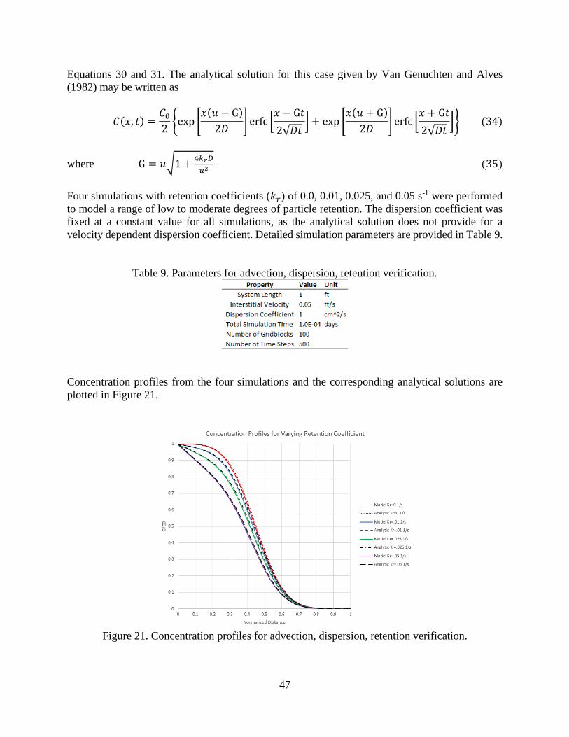
47

Equations 30 and 31. The analytical solution for this case given by Van Genuchten and Alves

(1982) may be written as

𝐶(𝑥, 𝑡) =𝐶0

2{exp [

𝑥(𝑢 − G)

2𝐷] erfc ⌊

𝑥 − G𝑡

2√𝐷𝑡⌋ + exp [

𝑥(𝑢 + G)

2𝐷] erfc ⌊

𝑥 + G𝑡

2√𝐷𝑡⌋} (34)

where G = 𝑢√1 +4𝑘𝑟𝐷

𝑢2 (35)

Four simulations with retention coefficients (𝑘𝑟) of 0.0, 0.01, 0.025, and 0.05 s-1 were performed

to model a range of low to moderate degrees of particle retention. The dispersion coefficient was

fixed at a constant value for all simulations, as the analytical solution does not provide for a

velocity dependent dispersion coefficient. Detailed simulation parameters are provided in Table 9.

Table 9. Parameters for advection, dispersion, retention verification.

Concentration profiles from the four simulations and the corresponding analytical solutions are

plotted in Figure 21.

Figure 21. Concentration profiles for advection, dispersion, retention verification.

48

Simulations for all four levels of retention coefficient were in close agreement with the analytical

solutions, providing confirmation that retention had been implemented accurately in the finite

difference simulator.

2.3.6. Radial Diffusion

To verify that the finite difference simulator was functional in multiple dimensions, a radial

diffusion case was modeled. If a cylindrical system is internally bound by a cylinder with radius r

= a and has the initial condition

𝐶(𝑟, 𝑡) = 0, 0 ≤ 𝑟 < ∞, 𝑡 > 0, (36)

and a boundary condition of

𝐶(𝑟, 𝑡) = 𝐶0, 𝑟 = 𝑎, 𝑡 > 0, (37)

then, as illustrated by Crank (1975), the analytical solution for concentration as a function of

radial distance and time may be written as

𝐶(𝑟, 𝑡) = 𝐶0 +2𝐶0

𝜋∫ exp(−𝐷𝑤2𝑡)

𝐽0(𝑤𝑟)𝑌0(𝑤𝑎) − 𝐽0(𝑤𝑎)𝑌0(𝑤𝑟)

𝐽02(𝑤𝑎) + 𝑌0

2(𝑤𝑎)

∞

0

d𝑤

𝑤 (38)

where 𝐽0 and 𝑌0 are Bessel functions of the first and second kind respectively. As further illustrated

by Crank (1975), Equation 38 may be approximated for small time values as

𝐶(𝑟, 𝑡) = 𝐶0 [(𝑎

𝑟)

1/2

erfc (𝑟 − 𝑎

2√𝐷𝑡) +

(𝑟 − 𝑎)(𝐷𝑡)1/2

4𝑎1/2𝑟3/2ierfc (

𝑟 − 𝑎

2√𝐷𝑡) (39)

+𝐷𝑡(9𝑎2 − 2𝑎𝑟 − 7𝑟2

32𝑎3/2𝑟5/2i2erfc (

𝑟 − 𝑎

2√𝐷𝑡) + ⋯ ]

where

ierfc(𝑥) = 1

𝜋1/2e−𝑥2

− 𝑥 erfc(𝑥) (40)

i2erfc(𝑥) = 1

4[erfc(𝑥) − 2𝑥 ierfc(𝑥)] (41)

A finite difference system was created to match the boundary condition of Equation 36 as closely

as possible. The system created was two-dimensional, contained 25 grid blocks in both the X and

Y directions, and had grid block side lengths of .01 feet in all directions. Due to the Cartesian basis

of the finite difference model, the radial boundary condition was approximated using a “stair step”

approach. Figure 22 depicts the lower 6 by 6 region of the 25 by 25 grid system, and illustrates

how the “stair step” approach was implemented.

49

Figure 22. “Stair step” boundary implementation.

A total of 10 grid blocks (red blocks in Figure 22) were kept at a concentration value of 𝐶0 during

the entire simulation. The radius of the internally bound cylinder, a, was calculated to be 0.357 ft.

This value was obtained by equating the area of a quarter circle with radius a to the area of the 10

grid blocks held at 𝐶0. Results for simulations using values of Dt/a2 of 0.25 and 1.0 are shown in

Figure 23.

Figure 23. Radial diffusion concentration profiles.

Given that the grid blocks of the finite difference simulator were defined in a Cartesian grid, it was

not possible to replicate a radial system exactly. Despite this limitation, the maximum percent error

between any concentration value given by the finite difference model and the corresponding value

given by the approximate analytical solution (Equations 39-41) was 7.06 percent. Due to this

50

favorable agreement with the approximate analytical solution, the finite difference simulator was

shown to be capable of accurately solving concentration fields in multi-dimensional systems.

2.3.7. Full Dispersion Tensor

A qualitative and quantitative analysis was performed to investigate the incorporation of the full

dispersion tensor into the finite difference simulator. In principle, it was necessary to incorporate

the full dispersion tensor as particle dispersion could occur in directions that were not aligned with

the principal directions of the Cartesian continuum-scale model. A series of simulations were

performed in which a single grid block at the center of a square two-dimensional system was held

at constant concentration C0. For all simulations, the system dimensions were 10ft by 10ft by 1 ft,

total simulated time was 1.0E-3 days and simulation time steps were 5.0E-5 days. Additionally,

all simulations were purely diffusive (no advection); however, the full dispersion tensor was

modified to cause anisotropic diffusion. As a base case, the first simulation modeled equivalent

dispersion in all directions. Thus, the dispersion coefficient aligned with the x direction, 𝐷𝑥𝑥, was

set equal to that in the y direction, 𝐷𝑦𝑦, and diagonal dispersion coefficients were set to zero. The

concentration field for the control simulation, which used 𝐷𝑥𝑥 = 𝐷𝑦𝑦 = 25.0 cm/s2 and 51 grids in

the X and Y directions, is shown in Figure 24.

Figure 24. Concentration field for equivalent dispersion in all directions.

The radially symmetric concentration field indicates that dispersion was equivalent in all

directions, which shows that the base case model was implemented correctly. The second

simulation reduced 𝐷𝑦𝑦 to 2.5 cm2/s (one order-of-magnitude) and kept 𝐷𝑥𝑥 at 25.0 cm2/s. Such a

dispersion tensor could occur when a high velocity flow field is aligned with the x direction. The

final concentration field for this simulation, performed on a 51 by 51 grid system, is shown in

Figure 25.

Grid n

um

ber

in y

direction

Grid number in x direction

10 20 30 40 50

5

10

15

20

25

30

35

40

45

50

C/C

0

0.1

0.2

0.3

0.4

0.5

0.6

0.7

0.8

0.9

1

51

Figure 25. Concentration field for dominant dispersion in x direction.

The elongated concentration profile in the x direction indicates that dispersion in the x direction is

indeed much larger than the y direction. The previous two simulations had dispersion tensors with

all off diagonal elements equal to zero, which served as a basis for comparison. If the velocity

vector of fluid flow in a grid cell is not aligned with one of the principal Cartesian directions, the

dispersion tensor effectively undergoes a rotation transformation. This transformation results in

non-zero off-diagonal elements of the dispersion tensor. To represent such a situation, two

additional simulations were performed in which the dispersion tensor of the second simulation

(dominant dispersion in X direction) was rotated. The two rotation transformations used were 20-

and 45-degree clockwise rotations. Dispersion tensors for all four simulations are summarized in

Table 10 (all dispersion values in cm2/s).

Table 10. Dispersion tensor values.

The final concentration fields for the rotated dispersion tensor simulations, performed on a 51 by

51 grid system, are shown in Figure 26.

Grid n

um

ber

in y

direction

Grid number in x direction

10 20 30 40 50

5

10

15

20

25

30

35

40

45

50

C/C

0

0

0.1

0.2

0.3

0.4

0.5

0.6

0.7

0.8

0.9

1

52

Figure 26. Concentration field for 20-degree (left) and 45-degree (right) rotation.

The superimposed red lines in Figure 26 depict 20-degree and 45-degree angles. For both cases,

the direction of maximum dispersion is aligned with the degree of rotation, which indicates the

finite difference solution correctly implemented the off-diagonal elements of the dispersion tensor.

Compared to the base case of Figure 25 however, the concentration fields in Figure 26 appear to

have lower concentration gradients in the transverse direction. Thus, rotation appears to artificially

cause additional dispersion in the transverse direction. This effect is likely due to the Cartesian

nature of the grid-based simulator. When a concentration front spreads along a direction that is not

one of the principal Cartesian directions, it cannot travel in a straight line. Instead the front must

take a “stair step” path, which will result in artificially high dispersion in the transverse direction

and artificially low dispersion in the longitudinal direction. This effect will be most pronounced

when the longitudinal flow direction is least aligned with a principal Cartesian direction. In a two-

dimensional system, this occurs at a 45-degree angle to the principal Cartesian directions. This

effect can be seen in Figure 26 as the ratio of longitudinal spreading to transverse spreading of

concentration is lowest for the 45-degree case.

This effect can be mitigated by increasing the grid refinement. To investigate, a series of

simulations were performed with the same parameters as simulations 3 and 4 in Table 10 but with

increasing numbers of finite difference grids. Simulations were performed for grid systems of 11

by 11 (121 grids), 51 by 51 (2,601 grids), 101 by 101 (10,201 grids), 251 by 251 (63,001), and

317 by 317 (100,489 grids). For each simulation, a concentration profile was recorded. For the 20-

degree rotation case, the concentration profile was taken from the system origin to the edge located

at x = 10ft, y = 5ft (middle of right edge). For the 45-degree rotation case, the concentration profile

was taken from the system origin to the corner located at x = 10ft, y = 10ft. Results for all

simulations are shown in Figures 27 and 28.

53

Figure 27. Concentration profiles for 20-degree rotation.

Figure 28. Concentration profiles for 45-degree rotation.

Concentration profiles for both simulations converge as the number of grid blocks used increases.

This implies that increasing grid refinement can reduce errors due to concentration fields spreading

in directions not aligned with the principal Cartesian directions of the system.

54

2.4. Concurrently Coupled Model

2.4.1. Concurrently Coupled Model Overview

The algorithm used to run the concurrently coupled simulator developed in this work is depicted

in Figure 29.

Figure 29. Algorithm for concurrently coupled particle transport and retention simulations.

Each finite difference grid block in the concurrently coupled model was first initialized with the

properties of the embedded PNMs (Step1). Each time step then began by solving the pressure field

(Step 2). In Step 3, the velocity flow field (derived from the pressure field) and the particle

concentration field were used to predict the number of particles (Np) for each particle species that

would enter each PNM during the time step. Simulations were then performed in Step 4 in which

the number of particles as predicted in Step 3 were used to damage each embedded PNM. In Step

5, simulations were performed in each grid block (distinct from those in Step 4) to determine the

continuum-scale properties of interest: permeability, porosity, retention coefficient, and dispersion

coefficient (longitudinal and transverse). Retention and dispersion coefficients were determined

for each particle species. These properties were then assigned to each finite difference grid block

(Step 6) and the concentration field was solved for (Step 7). The two-way transfer of information,

between the PNMs and continuum-scale grids (Steps 2 through 7), continued until the simulation

was complete (Step 8). It is important to note that the user could select the frequency at which

PNM property updates via PNM simulation occurred (Steps 3 through 6. This enabled high

temporal resolution for pressure and concentration field updates, which helped to reduce numerical

dispersion, while allowing the algorithm to run in a timely manner.

55

Chapter 3. Results and Discussion

3.1. One-Dimensional Concurrent Coupling

Simulations with gradually increasing size discrepancies between embedded pore-scale models

and finite difference grid blocks were run to identify potential challenges associated with the

concurrently coupled particle filtration model. Simulations with no size discrepancy between the

pore- and continuum-scale models, referred to in this work as 1-to-1 simulations, were first used

to ensure that the boundary condition and parameter coupling had been implemented correctly and

to evaluate the potential impact of numerical dispersion. These simulations were followed by

simulations involving finite difference grid blocks three times larger than their embedded PNMs.

The final one-dimensional concurrently coupled simulations involved finite difference grid blocks

eleven times larger than their embedded PNMs. Additional concurrently coupled simulations with

bidisperse particle systems were run at various pore- and continuum-scale size discrepancies. The

accuracy of each concurrently coupled simulation was validated by a boundary coupled simulation

with identical input parameters, such as particle concentration and system size. While the

concurrently coupled simulations generated particle concentration information using a finite

difference approximation to the modified version of the advection dispersion equation given by

Equation 3, boundary coupled simulations tracked the pore-to-pore transport of each individual

particle. The direct particle tracking of the boundary coupled simulations provided a fundamentally

reliable representation of overall particle transport behavior that was used to evaluate the accuracy

of the concurrently coupled simulations.

3.1.1. One-Dimension 1-to-1 Concurrent Coupling with No Retention

A series of one-dimensional simulations with no particle retention were used to verify that the

concurrently coupled model had been correctly developed. In the simulations, the continuum-scale

finite difference model occupied the same volume as the embedded PNMs. When the continuum-

and pore-scale models occupy the same volume and represent the same system, the behavior of

the concurrently coupled system should replicate the behavior of a system containing only

boundary coupled PNMs.

Simulations involving only boundary coupled PNMs were first run to serve as a basis for

comparison for the concurrently coupled model. The simulated systems consisted of 20 boundary

coupled PNMs. Injection of 50,000 particles at a constant rate into the system over 0.5 system pore

volumes was simulated. A particle diameter size of 0.01 microns was used for all particles to ensure

that they were too small to become trapped in the PNMs. In the simulations a constant flow rate

boundary condition, which corresponded to a Darcy velocity of 0.01 cm/s was imposed, together

with a constant fluid viscosity of 0.01 g/cm-s. At 0.5 pore volumes of injected fluid, particle

concentrations were calculated in each grid block. Simulations for these conditions used Berea

PNMs, random uniform (RU) PNMs, and Lattice PNMs. See section 2.1.1. for more information

on these PNM systems. The resulting particle concentration profile at 0.5 pore volumes for each

of the three PNM systems is shown in Figure 30.

56

Figure 30. Concentration profiles of 50,000 particles injected into 20 boundary coupled PNMs at

0.5 system pore volumes.

A comparison with the analytic solution for a constant injection concentration (Equations 34 and

35) was made to test the validity of the concentration profiles generated using the boundary

coupled PNM simulations. Values for longitudinal dispersion and retention coefficients are

required to generate the analytic solutions. These coefficients were obtained in separate

simulations that used the same boundary conditions as the previous simulations. Section 2.1.3.

provides details on the methods used to evaluate the dispersion coefficient. Dispersion coefficient

values of 1.0E-3 cm2/s, 1.2E-3 cm2/s, and 5.0E-4 cm2/s were calculated for the Berea PNM, RU

PNM, and Lattice PNM, respectively. Table 11 summarizes the parameters used in the analytical

solution for each PNM. Figures 31 to 33 provide comparisons of the boundary coupled

concentration profiles at 0.5 system pore volumes (Figure 30) to the analytical solutions using the

parameters from Table 11 for each PNM system.

Table 11. Parameters for analytical solution for concentration profiles of particles injected into

20 boundary coupled PNMs at 0.5 system pore volumes.

57

Figure 31. Analytical and simulated concentration profile of 50,000 particles injected into 20

boundary coupled PNMs at 0.5 system pore volumes (Berea PNM).

Figure 32. Analytical and simulated concentration profile of 50,000 particles injected into 20

boundary coupled PNMs at 0.5 system pore volumes (RU PNM).

58

Figure 33. Analytical and simulated concentration profile of 50,000 particles injected into 20

boundary coupled PNMs at 0.5 system pore volumes (Lattice PNM).

The qualitative agreement of the matches between the analytical and simulated concentration

curves provide support to the validity of the coefficient values. Additionally, because the simulated

boundary coupled PNM concentration profiles match the analytical solutions, it can be inferred

that, in the absence of retention, the PNM simulations produce physically realistic results

consistent with classical theory. Given that the continuum-scale model developed in this work uses

a finite-difference solution based on an approximate form of classical theory, it should therefore

be in agreement the boundary coupled PNM solution when accurate coefficient values are used

and numerical dispersion is small.

To verify that the finite difference model used by the concurrently coupled model could match the

boundary coupled PNM solutions for particle transport, a series of simulations using only the finite

difference model were performed (without embedded PNM simulations and coupling). These

simulations were run with varying spatial and temporal resolutions with the same system

parameters and boundary conditions of the previous boundary coupled PNM simulations. The

retention and dispersion coefficients used were those obtained from the PNM simulations

summarized in Table 11. Results for the three relevant dispersion coefficient values are shown in

Figures 34-36.

59

Figure 34. Concentration profiles for constant injection into 20 boundary coupled PNMs at 0.5

system pore volumes with finite difference solutions (Berea PNM).

Figure 35. Concentration profiles for constant injection into 20 boundary coupled PNMs at 0.5

system pore volumes with finite difference solutions (RU PNM).

60

Figure 36. Concentration profiles for constant injection into 20 boundary coupled PNMs at 0.5

system pore volumes with finite difference solutions (Lattice PNM).

When 20 finite difference grid blocks and ten time steps are used in the finite difference model,

numerical dispersion dominates the solution. This numerical dispersion is inherent to the finite

difference model and cannot be reduced by lowering the dispersion coefficient used. This is seen

in figures 34-36 where for all three cases the yellow curve, which uses the dispersion coefficients

in Table 11, is nearly identical to the purple curve, which has a finite-but-near-zero value for the

dispersion coefficient.

Numerical dispersion can be reduced by adding more finite difference grid blocks to the system

(total system size remaining constant) or by using more time steps in the finite difference model

(total simulated time remaining constant). The finite difference model approaches the boundary

coupled PNM solution when numerical dispersion is sufficiently reduced. For the Berea PNM and

RU PNM, 40 finite difference grid blocks and 200 time steps were sufficient to effectively

eliminate numerical dispersion. The Lattice PNM required 80 finite difference grid blocks and 400

time steps. Having a more uniform velocity distribution, the Lattice PNM had less physical

dispersion than the Berea PNM and RU PNM. A finer finite difference discretization is therefore

required relative to the Berea PNM and RU PNM to allow physical dispersion to dominate over

numerical dispersion.

The findings from the finite difference simulation comparisons indicate that a concurrently

coupled system with 20 finite difference grid blocks and 20 embedded PNMs of the same size will

be unable to match the 20 boundary coupled PNM solution. With that spatial discretization, the

finite difference solution of the continuum-scale model exhibited excessive numerical dispersion.

To overcome this limitation, it is possible to use different temporal and spatial discretizations for

the continuum-scale and PNM models.

61

Although the size of a PNM is fixed, multiple finite-difference grid blocks can be used to represent

the same amount of volumetric dimensions as a PNM in the coupled model. Each finite difference

grid block within the volume of the PNM would have the same values for retention and dispersion

coefficients, permeability, and porosity as the PNM. In a similar way, the finite difference time

steps can be smaller than the simulated time during a PNM simulation. The finite difference grid

block parameters remain constant at each small finite difference time step and are updated

periodically. Increasing spatial and temporal resolutions in this way provides a means of

effectively eliminating numerical dispersion for the sake of validation.

A series of simulations were performed to verify that the concurrently coupled model could

replicate the boundary coupled PNM solution for the case of equal system volumes and no

retention. For each PNM system (Berea, RU, and Lattice) a concurrently coupled simulation was

performed in which 20 finite difference grid blocks and 100 time steps were used to simulate 0.5

pore volumes of particles injected at a constant rate. Additional simulations were performed, which

used multiple finite difference grid blocks for each of the 20 PNMs in the concurrently coupled

model. The multiple finite difference grid blocks representing each PNM had equivalent

parameters derived from the single PNM they represented. The Berea and RU PNMs used a total

of 40 finite difference grid blocks and 200 time steps in the concurrently coupled model. In

comparison, the Lattice PNM used 80 finite difference grid blocks and 400 time steps. These

parameters were selected as they corresponded to levels of discretization in the finite difference

model, which effectively eliminated numerical dispersion in their respective PNM systems.

Results from the concurrently coupled simulations as well as the boundary coupled PNM and

finite-difference-only simulations are shown in Figures 37-39.

Figure 37. Concentration profiles for constant injection into 20 boundary coupled PNMs at 0.5

system pore volumes with finite difference and concurrently coupled solutions (Berea PNM).

62

Figure 38. Concentration profiles for constant injection into 20 boundary coupled PNMs at 0.5

system pore volumes with finite difference and concurrently coupled solutions (RU PNM).

Figure 39. Concentration profiles for constant injection into 20 boundary coupled PNMs at 0.5

system pore volumes with finite difference and concurrently coupled solutions (Lattice PNM).

63

These simulations demonstrate that, for the case of non-retaining particles, the concurrently

coupled simulator can produce accurate results when the continuum-scale model occupies the

same physical volume as the pore-scale model. The finite difference and concurrently coupled

simulations produce identical results because the system discretizations were the same and

parameter values for both were obtained from identical PNM simulations. The only difference was

that the finite difference only simulations obtained the parameters from the PNMs in separate

simulations, while the concurrently coupled model obtained the parameters from embedded PNMs

at each simulation time step. Although this scenario was simple in that a system without retention

has constant parameters, it shows that the concurrently coupled model can use boundary conditions

from the continuum-scale to obtain key parameters of interest from pore-scale models, and pass

these parameters back to finite difference grid blocks. Although limited in utility, because a

sequentially coupled PNM and continuum-scale finite difference model could produce the same

results as the concurrently coupled model, it served as a logical first step in this work.

3.1.2. One-Dimensional 1-to-1 Concurrent Coupling with Particle Retention

The advantage of using a concurrently coupled model becomes more evident in systems with

particle retention. Systems with retention have changing parameters, such as permeability,

porosity, and retention coefficient. The changes in these parameters are a complex function of

particle and matrix interactions that can only be accurately measured at the pore-scale. Although

experimental work can yield empirical functions of rock parameters, the accuracy of these

functions is limited to the experimental conditions (particle size distributions, injection rates, etc.)

used in the study. Using a concurrently coupled model allows for the measurement of changing

parameters under any simulated situation. Furthermore, because physically representative PNMs

can be generated for the specific system of interest, they have the potential to be more accurate

than experimentally derived data, which may come from systems other than that being

investigated.

A study was first performed to identify the conditions under which a 1-to-1 size concurrently

coupled model would be valid. To reiterate, a 1-to-1 size concurrently coupled model is one in

which the continuum-scale finite difference model occupies the same volume as the embedded

PNMs. When the continuum- and pore-scale models occupy the same volume and represent the

same system, the behavior of the concurrently coupled system should replicate that of a system

containing only boundary coupled PNMs.

1-to-1 concurrently coupled simulations may fail to replicate boundary coupled simulations due to

numerical dispersion. The boundary coupled simulations used in this study utilized a Lagrangian

particle tracking method that was not impacted by numerical dispersion. However, truncation

errors associated with the finite difference methods used by the concurrently coupled model caused

numerical dispersion. When numerical dispersion dominates physical dispersion, simulation

results become less accurate. This can occur if spatial resolutions or temporal resolutions are too

coarse. Figure 40 compares analytic and finite difference concentration profiles at 0.5 system pore

volumes injected for three cases with varying retention coefficients. The concentration profiles for

these and all other simulations involving particle retention in this work represent only the

concentration of non-trapped particles. For each simulation, 20 finite difference grid cells were

used and all rock parameters remained constant throughout the simulation. The finite difference

64

grid cell dimensions were set equal to those of the Berea PNM. A dispersion coefficient of 1.0 E-

3 cm2/s was used, and the 0.5 system pore volume injection time was discretized into 10 finite

difference time steps (each time step equivalent to the injection of one grid cell pore volume).

Figure 40. Analytic and finite difference concentration profiles at 0.5 system pore volumes with

varying retention coefficient.

At this level of discretization (20 finite difference grid cells and 10 time steps), when no retention

occurs (kr = 0.00 s-1), numerical dispersion causes significant error relative to the analytical

solution. As kr increases, the solution becomes dominated by the effect of retention and numerical

dispersion results in less deviation from the analytical solution. Increasing the temporal resolution

by adding more time steps (total simulated time held constant) reduces numerical dispersion.

Figure 41 compares simulation results for the cases of kr = 0.00 s-1 and kr = 0.05 s-1 with varying

numbers of time steps (10, 100, and 1,000) to analytical solutions.

65

Figure 41. Analytic and finite difference concentration profiles at 0.5 system pore volumes with

varying retention coefficient (varying temporal resolution).

Although numerical dispersion was reduced, it was not eliminated by increasing the temporal

resolution alone. This implies that a 1-to-1 system with 20 finite difference grid cells and 20

embedded PNMs of the same size may be unable to match an analytic or boundary coupled result

due to numerical dispersion. In general, concurrently coupled results will have more error due to

numerical dispersion when systems have low physical dispersion and low retention.

A series of simulations were performed on the same systems of Figure 41 to investigate the impact

of increasing spatial resolution on numerical dispersion. For all simulations 10 time steps were

used but the number of finite difference grid blocks was varied with total system length held

constant. Results for number of finite difference grids of 20, 200, and 2,000 compared to analytical

solutions are summarized in Figure 42.

66

Figure 42. Analytic and finite difference concentration profiles at 0.5 system pore volumes with

varying retention coefficient (varying spatial resolution).

Increasing the spatial resolution of the system had a negligible impact on numerical dispersion,

which remained significant when only 10 time steps were used. Thus, simply increasing either

spatial or temporal resolution alone does not ensure that numerical dispersion will be effectively

eliminated.

To evaluate if the numerical dispersion inherent to the concurrently coupled model developed in

this work was acceptable, a comparative simulation was performed using CMG’s IMEX, a widely

used commercial finite difference simulator with generally accepted numerical accuracy. The

scenario chosen for the comparison was the injection of a non-trapping solute species at uniform

injection concentration for 0.5 system pore volumes. The system was comprised of 20 finite

difference nodes with sizes and properties equivalent to the Berea PNM. For the concurrently

coupled model, given that no particles could be retained, system properties remained constant and

no PNM simulations were required to update system properties. The dispersion coefficient for the

solute species was set to zero so that any dispersion in the simulation would be due solely to

numerical dispersion. To create an identical simulation in CMG, a solute species was created by

using the SEAWATER feature. This feature allows for the injection of a non-reactive seawater

species. The properties of the injected seawater were made identical to the in-situ fluid, so the

seawater concentration was purely a solute species, with no impact on the rock or fluid system.

The input file for the CMG simulation containing all simulation parameters can be found in Figure

A1 of the Appendix. Results of the two simulations are shown in Figure 43.

67

Figure 43. Comparison of numerical dispersion to commercial simulator.

The finite difference simulator used in the concurrently coupled model of this work exhibited

significantly less numerical dispersion than the CMG model. The improved accuracy can be

attributed to the use of the QUICK upwinding scheme applied in this work. Given that the accuracy

of the finite difference model used in this work is on par with and potentially better than a widely

used commercial software, the numerical dispersion of the concurrently coupled model was

considered low enough given other potential sources of error, such as coefficient value accuracy.

A series of simulations were performed to confirm that numerical dispersion could be eliminated

at appropriate levels of spatial and temporal resolution. Simulations were performed with

increasing levels of spatial and temporal resolution (total simulated time and domain size held

constant) until a resolution was found that effectively eliminated numerical dispersion. The results

of these simulations are shown in Figure 44.

At sufficiently fine spatial and temporal resolutions, it was possible to effectively eliminate

numerical dispersion. Although the finite difference solutions shown in Figure 44 used a relatively

high resolution to eliminate numerical dispersion, acceptable accuracy was achieved with coarser

resolutions. Furthermore, systems with significant levels of retention require much less resolution

to eliminate numerical dispersion than systems without retention. Although updating parameters

with PNM simulations may be time consuming when performed at each finite difference time step

in a concurrently coupled simulation, parameter updates are only needed if a change in rock

parameters has occurred.

68

Figure 44. Analytic and finite difference concentration profiles at 0.5 system pore volumes with

varying retention coefficient (numerical dispersion eliminated).

The simulation results depicted in Figure 44 required spatial resolutions smaller than the length of

a single Berea PNM to reduce numerical dispersion. However, the ultimate goal of this work was

to simulate conditions in which the spatial resolution of the finite difference model was much

larger than the size of the embedded PNMs. As an intermediate step to this ultimate goal, a series

of simulations were performed to identify a 1-to-1 concurrently coupled system which had finite

difference grid cells equal in volume to their embedded PNMs, with low numerical dispersion.

From Figure 41 it can be seen that if there is no retention, a system of 20 finite difference grid cells

equal in size to the Berea PNM will exhibit significant numerical dispersion, even with very high

temporal resolutions. Simulations were performed in which the number of finite difference grid

cells was increased (grid cell size remaining constant) until numerical dispersion could be

effectively eliminated with a reasonable temporal resolution. Results for kr = 0.00 s-1 and kr = 0.05

s-1 are shown in Figures 45 and 46 respectively.

69

Figure 45. Analytic and finite difference concentration profiles at 0.5 system pore volumes for

finite difference grid sizes equal to Berea PNM dimensions (kr = 0.00 s-1).

Figure 46. Analytic and finite difference concentration profiles at 0.5 system pore volumes for

finite difference grid sizes equal to Berea PNM dimensions (kr = 0.05 s-1).

70

When kr = 0.00 s-1 and each finite difference grid was equivalent in size to a single Berea PNM,

increasing the number of finite difference grids alone could not eliminate numerical dispersion.

Although adding more finite difference grids reduced the effect of numerical dispersion, the

system length increased. A longer system length resulted in a sharper concentration front. In

practice, with a finite difference model, a sharper concentration front is more difficult to replicate

than a relatively more spread-out front because sharper fronts are more impacted by numerical

dispersion. Effectively this meant that the finite difference model, although second order accurate,

could not model without error a system with finite difference grid blocks of the same size and

dispersion coefficient as the Berea PNM, when kr = 0.00 s-1. Thus, the concurrently coupled model

would not be capable of producing error free predictions of concentration profiles under such 1-

to-1 model conditions. However, as shown in Figure 44, error free predictions could be made if

each embedded PNM was represented by multiple finite difference grid blocks. Alternatively, it

can be inferred that error free results could also be obtained if the Berea PNM was smaller in size.

In practice however, smaller PNMs are unsuitable as they contain fewer pores and tend to be less

representative of the true porous media compared to larger PNMs.

If retention is present, it is possible for numerical dispersion to be eliminated when each finite

difference grid is equivalent in size to a single Berea PNM. As can be seen in Figure 46, as the

number of finite difference grid cells was increased, numerical dispersion caused less and less

error. This research primarily considered cases where retention was non-zero. Thus, it was possible

to perform accurate modeling when the concurrently coupled model had finite difference grid

blocks that were the same size as their embedded PNMs. As particle trapping progresses however,

retention coefficients decrease. As retention coefficients decrease, numerical dispersion becomes

more dominant. Therefore, it was difficult to know a priori if an accurate simulation was possible

for a given 1-to-1 concurrently coupled system.

Simulations were performed to identify a situation with changing retention coefficient that could

be accurately modeled by a 1-to-1 concurrently coupled system with finite difference grids

equivalent in size to a single Berea PNM. A particle size of 10 microns was chosen for influent

damaging particles as this particle size became trapped in significant numbers in the Berea PNM.

Initially, the effect of 10-micron particle trapping on retention and dispersion coefficients for the

Berea PNM was investigated. Figures 47 and 48 demonstrate how these parameter values changed

as a function of the number of 10-micron particles trapped in a single Berea PNM.

71

Figure 47. Retention coefficient vs number of 10-micron particles retained in a single Berea

PNM.

Figure 48. Dispersion coefficient vs number of 10-micron particles retained in a single Berea

PNM.

For this particular PNM, at relatively small numbers of 10-micron particles retained (less than

about 200), retention coefficient decreased approximately linearly. Once the number of 10-micron

particles retained exceeds about 200 however, the retention coefficient decreased in a non-linear

fashion and could be approximated with a good degree of accuracy using a logarithmic model.

Dispersion coefficient in the Berea PNM was far less impacted by the retention of 10-micron

particles. Although its value fluctuated around an average of 1.02 E-3 cm2/s, its minimum and

maximum value differed by less than 10% for the case of 10-micron particles. Thus, for practical

72

purposes the dispersion coefficient of the Berea PNM was independent of the degree of 10-micron

particle trapping.

As an intermediate step towards running a 1-to-1 concurrently coupled model with PNMs,

simulations were performed that used a piecewise empirical equation to periodically update

retention coefficient in the case of 10-micron particle injection. Use of an empirical equation for

retention coefficient, although not possible in general, was faster than using a PNM simulation.

This aided in rapid testing of the concurrently coupled model. The piecewise empirical equation

used was obtained by replotting Figure 47 with number of particles injected as the independent

variable, rather than number of particles retained. The replotted version of Figure 47 is shown in

Figure 49.

Figure 49. Retention coefficient vs number of 10-micron particles injected into a single Berea

PNM.

The resulting piecewise empirical equation can be written as

‐ 2𝐸‐ 5𝑁𝑝 + 0.0937 if 𝑁𝑝 ≤ 500

𝑘𝑟 = ‐ 0.02 ln (𝑁𝑝) + 0.2106 if 500 ≤ 𝑁𝑝 ≤ 25,000 (42)

‐ 1𝐸‐ 7𝑁𝑝 + 0.0093 if 𝑁𝑝 > 25,000

where 𝑁𝑝 represents number of particles injected into a given PNM. When using Equation 42, a

minimum value of zero was used as a lower limit for values of 𝑁𝑝 larger than 100,000. Number of

particles injected was used as the independent variable as it is simpler to predict than number of

particles retained in a PNM.

73

Regardless of whether a PNM simulation or an empirical function was used to obtain grid block

properties, a formulation was required to determine 𝑁𝑝. For a given grid cell j and time step length

∆𝑡, 𝑁𝑝 (number of particles entering an embedded PNM) can be evaluated as

𝑁𝑝,𝑗 = 𝐶𝑗−ℓ𝑃𝑁𝑀/2 𝑄 ∆𝑡 (43)

where 𝑄 represents volumetric flow rate into the PNM and 𝐶𝑗−ℓ𝑃𝑁𝑀/2 (units of number of particles

per volume) represents particle concentration in block j evaluated at the upwind face of the

embedded PNM. It is important to note that 𝑁𝑝 is defined as the number of particles that enter the

PNM, not the grid block. Various methods are available for evaluating 𝐶𝑗−ℓ𝑃𝑁𝑀/2 and linear

interpolation between 𝐶𝑗 and 𝐶𝑗−1 was used, the accuracy of which was sufficient for the purpose

of this work. If the embedded PNM and finite difference grid blocks are the same size, then they

share the same face location and the number of particles entering the grid block is the same as that

entering the PNM. In this scenario equation 43 becomes

𝑁𝑝,𝑗 =𝐶𝑗 + 𝐶𝑗−1

2 𝑄 ∆𝑡 (44)

However, if the embedded PNM is smaller than the finite difference grid block, the number of

particles entering the PNM may be significantly different than the number of particles entering the

finite difference grid block over any given time step. Failure to evaluate 𝑁𝑝,𝑗 using the upwind

PNM face concentration can result in significant error, as Section 3.1.5. will demonstrate.

Importantly, before a given time step, all grid block parameters should be determined and these

parameters remain constant during the time step. If parameter values change over the course of a

time step, then use of a set of parameters that was valid only at the beginning of a time step can

lead to error. For example, particle retention may result in a lower value of retention coefficient at

the end of a time step compared to the beginning. Thus, applying the initial larger retention

coefficient value over that finite difference time step would lead to a predicted concentration value

in the grid block that would be too low. Similarly, if the finite difference model used the retention

coefficient value at the end of the time step, the predicted concentration value in the grid block

would be higher than the true value. Thus, it is better to evaluate parameter values at an

intermediate time between the beginning and end of a time step, and apply these intermediate

values over the duration of the time step. For this reason, this work used a value of 𝑁𝑝 evaluated

at a time halfway between the beginning and end of the time step to determine grid block parameter

values. This intermediate value of 𝑁𝑝, called 𝑁𝑝𝑖 in this work, can be evaluated for a given grid

cell j at a given time step n as

𝑁𝑝𝑖,𝑗 =1

2(∑ 𝑁𝑝,𝑗 + ∑ 𝑁𝑝,𝑗

𝑛+1

𝑡=0

𝑛

𝑡=0

) − ∑ 𝑁𝑝𝑖,𝑗

𝑛−1

𝑡=0

(44)

where the term in parentheses represents the cumulative number of particles injected half way

between the current and next time step, and the rightmost term represents the cumulative number

of particles previously injected into the grid cell.

74

As a basis of comparison for the concurrently coupled models, concentration profiles were

generated after 0.5 system pore volumes of injection of 10-micron-diameter particles into various

boundary coupled Berea PNM systems. The first set of simulations considered a total of 50,000

particles injected into 10, 20, and 40 boundary coupled Berea PNMs. For all cases, the particles

were injected at a constant rate and concentration over the 0.5 system pore volume period. The

concentration profiles for these simulations are shown in Figure 50.

Figure 50. Concentration profiles for injection of 50,000 10-micron particles into 10, 20, and 40

boundary coupled Berea PNMs at 0.5 system pore volumes.

It is important to note that concentration values in a given PNM should be evaluated using effective

rather than bulk pore volumes. In this work effective pore volume was calculated by summing the

pore volume of all pores which had non-zero inlet and outlet flow rates. The concentration within

a given PNM, 𝐶𝑃𝑁𝑀, normalized to inlet concentration, 𝐶0, was determined as

𝐶0 =𝑇𝑜𝑡𝑎𝑙 𝑁𝑢𝑚𝑏𝑒𝑟 𝑜𝑓 𝐼𝑛𝑗𝑒𝑐𝑡𝑒𝑑 𝑃𝑎𝑟𝑡𝑖𝑐𝑙𝑒𝑠

𝑇𝑜𝑡𝑎𝑙 𝑃𝑉 𝐼𝑛𝑗𝑒𝑐𝑡𝑒𝑑 [𝑐𝑚3] (45)

𝐶𝑃𝑁𝑀 =𝑁𝑢𝑚𝑏𝑒𝑟 𝑜𝑓 𝑝𝑎𝑟𝑡𝑖𝑐𝑙𝑒𝑠 𝑖𝑛 𝑃𝑁𝑀

𝐸𝑓𝑓𝑒𝑐𝑡𝑖𝑣𝑒 𝑃𝑁𝑀 𝑃𝑜𝑟𝑒 𝑉𝑜𝑙𝑢𝑚𝑒 [𝑐𝑚3] (46)

𝐶𝑃𝑁𝑀

𝐶0=

𝑁𝑢𝑚𝑏𝑒𝑟 𝑜𝑓 𝑝𝑎𝑟𝑡𝑖𝑐𝑙𝑒𝑠 𝑖𝑛 𝑃𝑁𝑀

𝐸𝑓𝑓𝑒𝑐𝑡𝑖𝑣𝑒 𝑃𝑁𝑀 𝑃𝑜𝑟𝑒 𝑉𝑜𝑙𝑢𝑚𝑒 [𝑐𝑚3]

𝑇𝑜𝑡𝑎𝑙 𝑃𝑉 𝐼𝑛𝑗𝑒𝑐𝑡𝑒𝑑 [𝑐𝑚3]

𝑇𝑜𝑡𝑎𝑙 𝑁𝑢𝑚𝑏𝑒𝑟 𝑜𝑓 𝐼𝑛𝑗𝑒𝑐𝑡𝑒𝑑 𝑃𝑎𝑟𝑡𝑖𝑐𝑙𝑒𝑠 (47)

As particles become retained, throat conductance values can become zero resulting in pores that

do not contribute to fluid flow in the system. These no flow pores contribute to bulk porosity but

75

not effective porosity. As more particle retention occurs, effective porosity decreases. If this effect

is not taken into account and bulk porosity is used to determine particle concentration values inside

a given PNM, the result will be artificially low values of grid block concentration.

To illustrate this point, solute flow simulations were run on two boundary coupled systems of 10

Berea PNMs. The first simulation used non-damaged Berea PNMs and the second simulation

involved Berea PNMs that had been damaged by a random mix of 100,000 10-micron-diameter

particles and 100,000 13-micron-diameter particles. In each simulation 10,000 solute particles

were injected over 0.8 system pore volumes. PNM concertation values in the two simulations were

evaluated using both bulk and effective porosity as the basis for PNM pore volume when

determining solute concentration values. Table 12 contains bulk and effective porosity values for

the two PNMs.

Table 12: Bulk and effective porosity values for undamaged and damaged Berea PNMs.

Both the undamaged and damaged Berea PNMs have the same bulk porosity. In the undamaged

PNM about 2% of pores do not contribute to flow resulting in an effective porosity value about

98% of the bulk porosity. Injection and retention of particles into the undamaged Berea PNM

resulted in reducing the effective porosity to about 93% of bulk porosity. Concentration profile

results from the two simulations are displayed in Figures 51 and 52.

76

Figure 51. Solute concentration profile comparison: undamaged Berea PNMs.

Figure 52. Solute concentration profile comparison: damaged Berea PNMs.

In the undamaged system there was little difference in bulk and effective porosity, which

corresponded to little difference in the concentration profiles calculated by both methods. On the

other hand, in the damaged system the concentration profile as evaluated using bulk porosity was

noticeably lower than that evaluated using effective porosity. Extrapolating the concentration

curves to the inlet, the value corresponding to the effective porosity formulation trended towards

1.0, while that determined by bulk porosity trended to below 1.0 (about 0.95). Given that the inlet

concentration should be 1.0, it can be inferred that effective porosity is the proper porosity to use

when evaluating PNM concentration values. If bulk porosity were used to determine PNM

77

concentrations, boundary coupled simulations with significant amounts of retained particles and

relatively lower effective porosities would have artificially low concentration values. This would

lead to artificial discrepancies between concurrently coupled simulations and boundary coupled

simulations with identical input parameters.

1-to-1 concurrently coupled simulations were performed and compared to the boundary coupled

results of Figure 50. The results of these simulations, shown in Figure 53, used the piecewise

empirical formula of Equation 42 to evaluate kr. For each system size, one concurrently coupled

simulation was performed in which the finite difference grid cells had the same size as a Berea

PNM, and a second concurrently coupled simulation was performed with an order-of-magnitude

higher spatial resolution.

Figure 53. Comparison of concentration profiles for injection of 50,000 10-micron particles into

10, 20, and 40 boundary coupled Berea PNMs at 0.5 system pore volumes with concurrently

coupled simulations (empirical formulation for kr).

The higher spatial resolution simulations had resolutions fine enough to effectively eliminate

numerical dispersion. Therefore, the spread between the high resolution and low resolution

concurrently coupled simulations was purely due to numerical dispersion. With 10 finite difference

grid cells, numerical dispersion was significant and caused the concurrently coupled model to

differ significantly from the high resolution and boundary coupled cases. As the number of finite

difference grid cells increased, the difference between the high and low resolution concurrently

coupled simulations decreased. Despite the effects of numerical dispersion, concurrently coupled

simulation results produced good qualitative matches for the cases of 20 and 40 boundary coupled

PNMs. As long as the error associated with using an empirical formulation for kr is small, a

78

concurrently coupled model using PNMs rather than the empirical formulation should also result

in good matches with boundary coupled simulations.

For completeness, simulations were performed which were identical to those shown in Figure 53,

with a total number of particles injected of 25,000 and 10,000 rather than 50,000. The results of

these simulations are shown in Figures 54 and 55. Simulations for 10 boundary coupled PNMs

were omitted due to the previously observed significant impact of numerical dispersion with only

10 finite difference grid cells.

Figure 54. Comparison of concentration profiles for injection of 25,000 10-micron particles into

20 and 40 boundary coupled Berea PNMs at 0.5 system pore volumes with concurrently coupled

simulations (empirical formulation for kr).

Figure 55. Comparison of concentration profiles for injection of 10,000 10-micron particles into

20 and 40 boundary coupled Berea PNMs at 0.5 system pore volumes with concurrently coupled

simulations (empirical formulation for kr).

79

As was the case for 50,000 particles, concurrently coupled simulations using finite difference grid

cells the same size as the Berea PNM and Equation 42 for kr were able to produce good qualitative

matches with boundary coupled simulations for 25,000 and 10,000 10-micron particles injected.

Simulations were performed to confirm that the concurrently coupled model using PNMs to update

coefficient values rather than the empirical formulation of Equation 42 could accurately match

boundary coupled simulation results. 1-to-1 concurrently coupled simulations using PNMs were

performed for a system size of 20 Berea PNMs and total number of 10-micron particles injected

of 50,000, 25,000, and 10,000. Results are summarized in Figure 56.

Figure 56. Comparison of concentration profiles for injection of 10-micron particles into 20

boundary coupled Berea PNMs at 0.5 system pore volumes with concurrently coupled

simulations.

The concurrently coupled simulations using PNMs to evaluate kr were able to replicate the

boundary coupled PNM simulation results with a high degree of accuracy. Discrepancies between

the concurrently coupled simulations using PNMs and the boundary coupled results can be

attributed to numerical dispersion. Evidence of this discrepancy can be inferred from Figure 56 as

concurrently coupled simulations with fewer particles injected more closely repreoduced the

boundary coupled results. When fewer particles were injected, fewer particles damage the system

and retention coefficients remained larger. Larger retention coefficients correspond to solutions

more dominated by retention and less influenced by numerical dispersion. Also, when relatively

large numbers of particles were injected and retained (as in the case of 50,000 particles injected)

retention coefficients were reduced to almost zero and numerical dispersion caused additional

80

error. Discrepancies between the concurrently coupled simulations using PNMs and those using

the empirical formulation to calculate kr can be attributed to error in the empirical formulation.

The results of Figure 56 demonstrate that a concurrently coupled model can use embedded PNMs

to accurately evaluate grid block properties and simulate particle transport and retention. Particle

retention in those simulations caused grid block properties to vary significantly in time and space.

An analytic solution or finite difference model with constant parameters would have been unable

to reproduce the boundary coupled results. Although, as was demonstrated, accurate finite

difference simulation results can be obtained when empirical formulations are used to evaluate

grid block properties, these formulations are time consuming to produce, not entirely accurate, and

most importantly are limited by the precise set of conditions used in their creation.

It is important to note that the single coefficient retention model of Equation 3 governs particle

transport and retention in the concurrently coupled model. Although previous experimental work

has shown this model to be deficient in scenarios in which size exclusion is the dominant

mechanism for retention, it provided accurate results in the 1-to-1 scenario. The improved accuracy

of the model can be attributed to the use of PNM simulations to periodically update the retention

coefficient in each finite difference grid block. Thus, the concurrently coupled model was able to

accurately simulate particle transport and retention in a straining dominated scenario without the

use of additional empirical parameters needed for alternate models, such as those of Tufenkji and

Elimelech (2004) and Porubcan and Xu (2010). This demonstrates the potential for concurrent

coupling to provide a flexible and simple means of simulating particle transport and retention.

3.1.3. One-Dimensional 3-to-1 Concurrent Coupling – Single Particle Size

Having demonstrated the accuracy of the 1-to-1 concurrently coupled model, the next stage of

model development focused on scenarios where the underlying PNMs were smaller than their

embedded grid blocks. For the concurrently coupled model to be useful for practical situations, the

embedded PNMs ultimately have to be significantly smaller than the finite difference grid blocks.

As discussed previously, PNMs are typically on the order of centimeters in length while finite

difference grid blocks in most systems of interest are on the order of meters. A series of simulations

were conducted to investigate the challenges and accuracy of concurrently coupled models with

such large size discrepancies.

As an intermediate step to simulating particle transport and retention in a concurrently coupled

system with order-of-magnitude differences in size between embedded PNMs and finite difference

grid blocks, a series of simulations were performed with small differences in size between the

pore- and continuum-scale models. The first system chosen was one-dimensional and contained

10 finite difference grid cells. Each grid cell had a PNM embedded in its center, with the length of

the PNM in the direction of flow being one-third that of the grid cell. Dimensions of the PNM in

non-flow directions were equivalent to the finite difference grid cells. Given the three-to-one size

ratio of grid cells to PNMs, this system will be referred to as a 3-to-1 system. A single grid cell

and embedded PNM for the 3-to-1 concurrently coupled system is depicted in Figure 57.

Before running concurrently coupled simulations on the 3-to-1 system, a baseline was obtained by

running a boundary coupled simulation of 30 Berea PNMs (equivalent system size to the 3-to-1

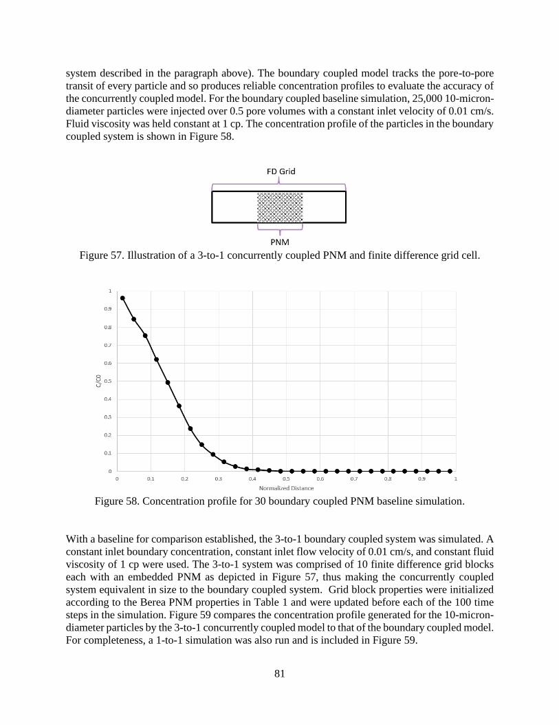
81

system described in the paragraph above). The boundary coupled model tracks the pore-to-pore

transit of every particle and so produces reliable concentration profiles to evaluate the accuracy of

the concurrently coupled model. For the boundary coupled baseline simulation, 25,000 10-micron-

diameter particles were injected over 0.5 pore volumes with a constant inlet velocity of 0.01 cm/s.

Fluid viscosity was held constant at 1 cp. The concentration profile of the particles in the boundary

coupled system is shown in Figure 58.

Figure 57. Illustration of a 3-to-1 concurrently coupled PNM and finite difference grid cell.

Figure 58. Concentration profile for 30 boundary coupled PNM baseline simulation.

With a baseline for comparison established, the 3-to-1 boundary coupled system was simulated. A

constant inlet boundary concentration, constant inlet flow velocity of 0.01 cm/s, and constant fluid

viscosity of 1 cp were used. The 3-to-1 system was comprised of 10 finite difference grid blocks

each with an embedded PNM as depicted in Figure 57, thus making the concurrently coupled

system equivalent in size to the boundary coupled system. Grid block properties were initialized

according to the Berea PNM properties in Table 1 and were updated before each of the 100 time

steps in the simulation. Figure 59 compares the concentration profile generated for the 10-micron-

diameter particles by the 3-to-1 concurrently coupled model to that of the boundary coupled model.

For completeness, a 1-to-1 simulation was also run and is included in Figure 59.

82

Figure 59. Concentration profile comparison of 3-to-1 and boundary coupled simulations.

The 3-to-1 concurrently coupled simulation results compared favorably with those of the boundary

coupled model, indicating that the changes in grid cell properties were properly calculated and

updated by the embedded PNMs. While promising, the result could have been achieved using an

empirical formulation for network properties due to the fact that a single particle size was used in

the simulation. The utility of the concurrently coupled model was evaluated by using more

complex simulations involving multiple particles sizes.

3.1.4. One-Dimensional 3-to-1 Concurrent Coupling – Multiple Particle Sizes

Given that many systems involving particle transport and retention involve particles with multiple

sizes, the multi-species capabilities of the concurrently coupled model were tested. The ability to

flexibly handle multiple particle species is a key advantage of concurrently coupled simulators.

Traditional finite difference models rely on empirical formulations of key parameters to determine

updated grid block properties. Although this is possible for single particle size systems, as was

demonstrated in section 2.4.3, it is highly impractical for multi-particle size systems. To investigate

this and highlight the benefit of using a concurrently coupled model, preliminary simulations were

run on a single Berea PNM to investigate the impact of different particle sizes and sequences on

particle transport and retention behavior.

The simplest multi-size particle system, that of two different particles sizes, was used in the

simulations. These two-particle size simulations are referred to as A/B simulations in this work

representing the two sizes. In the first A/B simulation, 10,000 7-micron-diameter particles were

injected into a single Berea PNM over two network pore volumes, immediately followed by 10,000

10-micron-diameter particles over an additional two pore volumes. The resulting effluent

concentration curve is shown in Figure 60. Simulation results are summarized in Table 13.

83

Figure 60. Effluent concentration curves for 10,000 7-micron-diameter particles followed by

10,000 10-micron-diameter particles into a Berea PNM.

Table 13. Particle retention summary for Figure 60.

Particle Diameter (microns)

Number Injected

Number Retained

Percent Retained

Retention Coefficient (1/s)

7 10,000 0 0.0 0

10 10,000 2,380 23.8 8.91E-02

None of the 7-micron-diameter particles were retained while 23.8% of the subsequent 10-micron-

diameter particles were retained in the Berea PNM. Throat radii of the Berea PNM were analyzed

to investigate the absence of retention of the 7-micron-diameter particles. A histogram of the throat

diameter of curvatures (TDC) for each throat in the PNM is provided in Figure 61, where a TDC

is defined as the tightest diameter of curvature, as measured by the smallest inscribed sphere that

can pass through a throat.

84

Figure 61. Histogram of throat diameter of curvatures for the Berea PNM.

It is clear that none of the seven micron particles were retained in the previous simulation because

no throats were small enough for them to become trapped. The unrealistic features of the throat

TDC histogram, such as the lack of throats with TCD values between zero and nine microns, is

likely a consequence of the finite resolution of the microtomography image used to create the

Berea PNM. Despite the limitations of the three-dimensional digital imaging and network

generation process, the Berea PNM was still valid for investigating particle transport and retention.

The subsequent A/B simulation was identical to that run previously, however the 10-micron-

diameter particles were injected first and the 7-micron-diameter particles were injected therafter.

Effluent concentration curves and the simulation result summary are shown in Figure 62 and Table

14 respectively.

85

Figure 62. Effluent concentration curves for 10,000 10-micron-diameter particles followed by

10,000 7-micron-diameter particles into a Berea PNM.

Table 14. Particle retention summary for Figure 62.

Particle Diameter (microns)

Number Injected

Number Retained

Percent Retained

Retention Coefficient (1/s)

10 10,000 2,338 23.4 8.76E-02

7 10,000 473 4.7 1.08E-02

The injection of 10-micron-diameter particles led to an increase in the retention of seven micron

particles from zero to about five percent. This demonstrates that for certain situations, particle

sequence can impact transport and retention behavior. For the sake of completeness, an additional

A/B simulation was performed which was identical to the first two, with the modification that

injection of 14-micron-diameter particles was followed by the injection of 7-micron-diameter

particles. Effluent concentration curves and the simulation result summary are shown in Figure 63

and Table 15 respectively.

86

Figure 63. Effluent concentration curves for 10,000 14-micron-diameter particles followed by

10,000 7-micron-diameter particles into a Berea PNM

Table 15. Particle retention summary for Figure 63.

Particle Diameter (microns)

Number Injected

Number Retained

Percent Retained

Retention Coefficient (1/s)

14 10,000 9,974 99.7 1.77

7 10,000 2,678 26.8 1.03E-1

Nearly all of the relatively large 14-micron-diameter particles were retained in the PNM, which

led to over 25% of the 7-micron particles being retained. Thus, both the size and sequence of

particles entering a porous medium can have a significant impact on the transport and retention of

those particles. While particle size and sequence can clearly impact transport behavior, the

previous A/B simulations involved particle sizes that resulted in particles which were nearly all

retained or all passed through the Berea PNM.

A second set of A/B simulations was performed to investigate the magnitudes of the impacts of

particle size and sequence on transport behavior. To this end, A/B simulations were performed

using more moderate particle diameters of 10 and 13 microns. A series of three A/B simulations

were performed on the Berea PNM. These three A/B simulations will be referred to as Cases A,

B, and C and are described in table 16.

87

Table 16. A/B simulation descriptions for cases A, B, and C. Simulation Case Description

A 15,000 10-micron-diameter particles injected over 3 PNM pore volumes, followed by 15,000 13-micron-diameter particles injected over an additional 3 PNM pore volumes. Particles injected into Berea PNM.

B 15,000 13-micron-diameter particles injected over 3 PNM pore volumes, followed by 15,000 10-micron-diameter particles injected over an additional 3 PNM pore volumes. Particles injected into Berea PNM.

C 15,000 10-micron-diameter particles and 15,000 13-micron-diameter particles injected together over 6 PNM pore volumes. Particles injected into Berea PNM.

For all three cases, particles were injected at constant concentrations. For Case C, the 10 and 13-

micron-diameter particles were mixed randomly. Effluent concentration curves for Cases A, B,

and C are provided in Figures 64-66 and retention results are summarized in Table 17.

Figure 64. Effluent concentration curves for Case A: 15,000 10-micron-diameter particles

followed by 15,000 13-micron-diameter particles injected into a Berea PNM.

88

Figure 65. Effluent concentration curves for Case B: 15,000 13-micron-diameter particles

followed by 15,000 10-micron-diameter particles injected into a Berea PNM.

Figure 66. Effluent concentration curves for Case C: 15,000 10-micron-diameter particles and

15,000 13-micron-diameter particles mixed injection into a Berea PNM.

89

Table 17. A/B simulation results summary for cases A, B, and C.

Simulation Case

Percent 10-micron-diameter Particles Retained

Percent 13-micron-diameter Particles Retained

A 20.2 90.1

B 38.2 92.4

C 41.8 87.3

The smaller particle species had more than double the extent of retention in case C compared to

case A. Although the larger particle size showed a smaller change in retention behavior, cases B

and C differed in the number of trapped particles by 5.7%, a non-negligible amount. Particle size

should therefore be appropriately incorporated into particle transport and retention models in order

for them to be accurate.

Logical arguments can be made to explain the behavior of cases A and B, however the behavior

of case C demonstrates the complexity of particle transport and retention. In case A, the smaller

particles were injected first and likely plugged smaller throats, diverting the flow field into more

of the larger throats. This likely led to the large particles subsequently injected in case A flowing

into more large throats with less overall retention of the larger particle species. In case B, the

injection of a larger particle species first resulted in greater retention of the smaller species. The

larger particles likely became trapped in throats that the smaller particles would normally have

been able to pass through, which reduced their throat sizes, leading to the observed greater

retention of the larger species. Interestingly, the mixed injection in case C led to the largest

retention of smaller particles and the least retention of the larger particles amongst cases A, B, and

C. The retention behavior of particles therefore cannot simply be interpolated from more extreme

cases of particle injection sequencing like cases A and B. This highlights the fact that particle

transport and retention is fundamentally a pore-scale phenomenon. Models that incorporate pore-

scale effects directly, such as concurrently coupled models, will have significant advantages over

those that do not, such as traditional finite difference based models based on the ADE.

To verify that the results of cases A, B, and C were not unique to the PNM model used, two

additional sets of A/B simulations were performed, one on a damaged version of the Berea PNM,

and one on the RU PNM described in Section 2.1.1. To alter the Berea PNM, 15,000 13-micron-

diameter particles (a size that becomes retained at a high rate) were injected into the Berea PNM.

The resulting altered PNM is referred to as the damaged Berea PNM. The three A/B simulations

run on the damaged Berea PNM are referred to as cases D, E, and F, and are described in table 18.

90

Table 18. A/B simulation descriptions for cases D, E, and F

Simulation Case Description

D

10,000 10-micron-diameter particles injected over 2 PNM pore volumes, followed by 10,000 13-micron-diameter particles injected over an additional 2 PNM pore volumes. Particles injected into Berea PNM previously damaged by 15,000 13-micron-diameter particles.

E

10,000 13-micron-diameter particles injected over 2 PNM pore volumes, followed by 10,000 10-micron-diameter particles injected over an additional 2 PNM pore volumes. Particles injected into Berea PNM previously damaged by 15,000 13-micron-diameter particles.

F 10,000 10-micron-diameter particles and 10,000 13-micron-diameter particles injected together over 4 PNM pore volumes. Particles injected into Berea PNM previously damaged by 15,000 13-micron-diameter particles.

As with cases A, B, and C, particles were injected at constant concentrations. For Case F, the 10

and 13-micron-diameter particles were mixed randomly. Effluent concentration curves for Cases

D, E, and F are provided in Figures 67-69 and retention results are summarized in Table 19, which

includes cases A, B, and C for comparison.

Figure 67. Effluent concentration curves for Case D: 10,000 10-micron-diameter particles

followed by 10,000 13-micron-diameter particles injected into a Berea PNM.

91

Figure 68. Effluent concentration curves for Case E: 10,000 13-micron-diameter particles

followed by 10,000 10-micron-diameter particles injected into a Berea PNM.

Figure 69. Effluent concentration curves for Case F: 10,000 10-micron-diameter particles and

10,000 13-micron-diameter particles mixed injection into the damaged Berea PNM.

92

Table 19. A/B simulation results summary for cases A through F.

Simulation Case

Percent 10-micron-diameter Particles Retained

Percent 13-micron-diameter Particles Retained

A 20.2 90.1

B 38.2 92.4

C 41.8 87.3

D 43.4 56.1

E 35.4 66.5

F 40.5 60.7

With a significant amount of particle trapping having already taken place in the damaged Berea

PNM, the amount of retained 10 and 13-micron-diameter particles was closer in cases D, E, and F

compared to cases A, B, and C. Although the sequence and sizes of particles in cases D, E, and F

mimicked cases A, B, and C, the relative retention of the cases differed significantly. For example,

case A showed the lowest amount of 10-micron particle retention amongst cases A, B, and C. As

with case A, case D had 10-micron particles being injected first, however the 10-micron particles

exhibited the greatest amount of retention amongst cases D, E, and F. This further demonstrates

the need for pore-scale modeling, as relative retention behaviors can change within a single system

as that system’s properties change.

A final set of A/B simulations for testing purposes were run on the RU PNM. As with cases A

though F, two particle sizes were selected that would exhibit moderately low and moderately large

amounts of retention. To identify appropriate particle sizes, the throat diameters of curvature of

the RU PNM system, plotted as a histogram in Figure 70, were analyzed.

Figure 70. Histogram of throat diameter of curvatures for the RU PNM.

93

Given the that the RU PNM was made of a random packing of spheres, its throat size distribution

follows a smooth log-normal distribution. Upon analysis of the distribution, particle diameters of

70 microns (mostly non-trapping) and 85 microns (moderately likely to trap) were selected for use

in the A/B simulations. Three simulations were run on the RU PNM with similar parameters to

cases D, E, and F. Descriptions of the A/B simulations run on the damaged RU PNM, referred to

as cases G, H, and I are provided in table 20.

Table 20. A/B simulation descriptions for cases E, F, and G.

Simulation Case Description

G 10,000 70-micron-diameter particles injected over 2 PNM pore volumes, followed by 10,000 85-micron-diameter particles injected over an additional 2 PNM pore volumes. Particles injected into the RU PNM.

H 10,000 85-micron-diameter particles injected over 2 PNM pore volumes, followed by 10,000 70-micron-diameter particles injected over an additional 2 PNM pore volumes. Particles injected into the RU PNM.

I 10,000 70-micron-diameter particles and 10,000 85-micron-diameter particles injected together over 4 PNM pore volumes. Particles injected into the RU PNM.

Effluent concentration curves for Cases G, H, and I are provided in Figures 71-73 and retention

results are summarized in Table 21, which includes cases A through F for comparison.

Figure 71. Effluent concentration curves for Case G: 10,000 70-micron-diameter particles

followed by 10,000 85-micron-diameter particles injected into the RU PNM.

94

Figure 72. Effluent concentration curves for Case H: 10,000 85-micron-diameter particles

followed by 10,000 70-micron-diameter particles injected into the RU PNM.

Figure 73. Effluent concentration curves for Case I: 10,000 70-micron-diameter particles and

10,000 85-micron-diameter particles mixed injection into the RU PNM.

95

Table 21. A/B simulation results summary for cases A through I.

Simulation Case

Percent of Smaller Particle Species Retained (10-

micron-diameter for cases A-F, 70-micron-diameter for

cases G-I)

Percent of Larger Particle Species Retained (13-

micron-diameter for cases A-F, 85-micron-diameter for

cases G-I)

A 20.2 90.1

B 38.2 92.4

C 41.8 87.3

D 43.4 56.1

E 35.4 66.5

F 40.5 60.7

G 17.9 86.3

H 34.4 87.5

I 30.1 86.5

The retention results for cases G, H, and I are different from those of A, B, and C and D, E, and F

in regard to the relative amounts of retention for the different sequences of smaller and larger

particles. More specifically, case H was the only case in which the injection of the larger particle

first resulted in the highest amount of small particle species retention. Also, cases G, H, and I

exhibited little difference in the retention behavior of the larger species compared to cases A, B,

and C and cases D, E, and F. Therefore, particle size and sequence were seen to impact multiple

porous media samples, which provides evidence that these parameters should be accounted for in

a wide range of, if not all, systems in which particle transport and retention is being modeled.

The A/B simulations above demonstrate that particle size, number, and sequence can have

significant impacts on particle transport behavior. For a traditional finite difference simulator to

accurately account for these parameters an empirical formulation would need to be made for an

effectively infinite combination of particle sizes, sequences, and amounts. This poses a significant

limitation in the ability of traditional finite difference simulators to accurately model particle

transport and retention. While this limitation was demonstrated for the simplest of multi-particle

systems, the situation becomes even more intractable for systems with more than two particle sizes.

While boundary coupled PNM simulations can easily handle multiple particle sizes, they are very

limited in scale. On the other hand, concurrently coupled models enable system sizes at practical

scales and the ability to accurately simulate multi-particle size systems in a computationally

efficient manner.

To remove the effects of the digital imaging process (which gave discrete pore and throat sizes)

for subsequent simulations, a portion of the throats with TDC values between 13 and 15 microns

were adjusted so that the TDC distribution would more closely follow a log-normal distribution.

Figure 74 shows the adjusted TDC histogram for the Berea PNM and Figure 75 compares the

original and adjusted values to a log-normal distribution. Although Figure 75 should technically

be plotted as a histogram, for the sake of simpler interpretation it is displayed as an XY scatter plot

with lines.

96

Figure 74. Histogram of throat diameter of curvatures for the adjusted Berea PNM.

Figure 75. Comparison of throat diameter of curvature distributions of the original and adjusted

Berea PNM to a log-normal distribution.

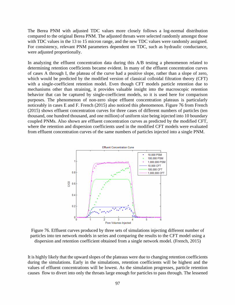
97

The Berea PNM with adjusted TDC values more closely follows a log-normal distribution

compared to the original Berea PNM. The adjusted throats were selected randomly amongst those

with TDC values in the 13 to 15 micron range, and the new TDC values were randomly assigned.

For consistency, relevant PNM parameters dependent on TDC, such as hydraulic conductance,

were adjusted proportionally.

In analyzing the effluent concentration data during this A/B testing a phenomenon related to

determining retention coefficients became evident. In many of the effluent concentration curves

of cases A through I, the plateau of the curve had a positive slope, rather than a slope of zero,

which would be predicted by the modified version of classical colloidal filtration theory (CFT)

with a single-coefficient retention model. Even though CFT models particle retention due to

mechanisms other than straining, it provides valuable insight into the macroscopic retention

behavior that can be captured by single-coefficient models, so it is used here for comparison

purposes. The phenomenon of non-zero slope effluent concentration plateaus is particularly

noticeably in cases E and F. French (2015) also noticed this phenomenon. Figure 76 from French

(2015) shows effluent concentration curves for three cases of different numbers of particles (ten

thousand, one hundred thousand, and one million) of uniform size being injected into 10 boundary

coupled PNMs. Also shown are effluent concentration curves as predicted by the modified CFT,

where the retention and dispersion coefficients used in the modified CFT models were evaluated

from effluent concentration curves of the same numbers of particles injected into a single PNM.

Figure 76. Effluent curves produced by three sets of simulations injecting different number of

particles into ten network models in series and comparing the results to the CFT model using a

dispersion and retention coefficient obtained from a single network model. (French, 2015)

It is highly likely that the upward slopes of the plateaus were due to changing retention coefficients

during the simulations. Early in the simulations, retention coefficients will be highest and the

values of effluent concentrations will be lowest. As the simulation progresses, particle retention

causes flow to divert into only the throats large enough for particles to pass through. The lessened

98

particle retention at the end of the simulation leads to higher effluent concentrations and an overall

upwards sloping effluent concentration profile. The effect is moderate in the simulation with

10,000 particles and very significant in the simulation with 100,000 particles. Thus, the more

significant slope in the 100,000 particle case was likely due to a greater change in retention

coefficient. The effect is muted in the simulation with 1,000,000 particles likely because the large

number of particles caused the retention coefficient to approach zero rapidly, from where it could

not change significantly. As can be seen in the 100,000 case, the effluent concentration is nearly

1.0 at the end of the simulation. This implies that the retention concentration was nearly zero after

approximately 0.4 pore volumes (100,000 particles injected) for the 1,000,000 particle case. The

effluent concentration curve approaching 1.0 approximately 0.4 pore volumes after breakthrough

for the 1,000,000 particle case supports this inference.

This phenomenon has important consequences. Firstly, retention coefficients should be evaluated

at specific points in time, not by fitting CFT models to raw effluent concentration curves. If the

latter approach is used, retention coefficient values may not be accurate because 1) CFT modified

with single-coefficient retention models predict zero slope effluent concentration profiles while

effluent concentration curves can have a slope and 2) the value of the retention coefficient may

change from the beginning of the simulation in a non-linear manner, making it difficult to identify

at what point the computed value actually represented the system. As discussed in Section 2.1.3.,

this work evaluates retention coefficients as specific points in time by determining the number of

particles that would become retained in the system, but does not actually retain those particles or

alter the system when doing so. Thus, when determining the retention coefficient in this work the

system does not change, which enables the retention coefficient to remain constant. Attempting to

determine the retention coefficient in a manner that alters the system, such as using an effluent

concentration curve from a particle retention simulation, will lead to artificially low values of

retention coefficient. The greater the number of particles used to evaluate the retention coefficient,

the lower the value will be. This is due to the fact that retention coefficients trend to zero as all

throats that are too small for particles to become trapped get plugged and flow is diverted such that

only throats large enough for particles to pass through remain. Thus although large numbers of

particles may be used to achieve statistical significance, this will make the calculated value more

precise but artificially low. Evidence of this can be seen in the 10,000 particle case (blue data set)

in Figure 76, where an artificially low value of retention coefficient likely led to the modified CFT

model under-predicting the amount of particle retention. Critically, because the concurrently

coupled model developed in this work evaluates retention coefficients at specific points in time, it

has the ability to calculate retention coefficients as frequently as needed. This ability would be

needed any time the retention coefficient changed rapidly. For example, if the retention coefficient

changed by 10% after just 100 particles were injected, the retention coefficient could be accurately

determined by the model in this work. However, an effluent concentration curve based on so few

particles would likely have a large amount of noise, leading to an inaccurate retention coefficient

value. Although retention coefficients were the focus of this discussion, similar arguments could

be made for any dynamic property derived from a pore-scale model.

Having established that particle size and sequence can have a material impact on transport and

retention, 3-to-1 concurrently coupled simulations were performed to test the model for accuracy

in evaluating these parameters. Two 3-to-1 concurrently coupled A/B simulations were run in

addition to the previous 3-to-1 simulation with a single particle size. The two additional

99

simulations involved particles of 10 and 13-micron-diameters. To make the results of the A/B

simulations comparable to those of Section 3.1.3., the same non-particle simulation parameters

(boundary flow rate, fluid viscosity, and system length) were used. Descriptions of the three A/B

3-to-1 simulations are provided in Table 22.

Table 22. A/B simulation descriptions for 3-to-1 concurrently coupled simulation cases.

Simulation Case Description

2A 25,000 10-micron-diameter particles injected over 0.5 system pore volumes. Particles injected into 10 3-to-1 finite difference grid cells each embedded with a Berea PNM (identical simulation to that in Section 2.4.3).

2B

25,000 13-micron-diameter particles injected over 0.5 system pore volumes, followed by 25,000 10-micron-diameter particles injected over an additional 0.5 PNM pore volumes. Particles injected into 10 3-to-1 finite difference grid cells each embedded with a Berea PNM.

2C 25,000 10-micron-diameter particles and 25,000 13-micron-diameter particles injected together over 0.5 system pore volumes. Particles injected into 10 3-to-1 finite difference grid cells each embedded with a Berea PNM.

As with the single particle size 3-to-1 case shown in Figure 58, boundary coupled simulations were

run for each case to obtain results to which the concurrently coupled models could be compared.

The boundary coupled simulations involved 30 Berea PNMs to make the system equivalent in size

to the 3-to-1 case. Concentration profiles of the 10-micron-diameter particles for each boundary

coupled simulation are plotted in Figure 77. For the sake of comparison, the concentration profiles

were taken after 0.5 pore volumes of injection of the 10-micron-diameter particle species. This

corresponded to simulation times of 0.5 pore volumes for cases 2A and 2C, and 1.0 pore volumes

for case 2B.

Figure 77. 10-micron particle species concentration profiles for 30 boundary coupled PNM

baseline simulations for cases 2A, 2B and 2C.

100

Noticeable differences in the concentration profiles for the 10-micron particles were observed in

the baseline PNM results. The differences in these profiles are due solely to the order in which the

two particle sizes entered the system. Qualitatively, the behavior of cases 2A and 2C match that

observed in the experimental work of Xu and Saiers (2009), which investigated the transport of

single and bidisperse particle suspensions. Xu and Saiers (2009) noted that the extent of retention

for the smaller particle species in the monodisperse case (2A in this work) was less than that in the

bidisperse case (2C in this work). Xu and Saiers (2009) attributed the increased retention of the

smaller species in the mixed case to the larger species partially constricting pore throats that the

smaller species would have otherwise been able to pass through. The ability of the boundary

coupled model to achieve a qualitative match with comparable experimental data provides

evidence that the straining rules implemented by the PNM were physically realistic.

As previously discussed, such results would be very difficult to model with a traditional finite

difference simulator based on the ADE. Such a model would need to rely on complex empirical

formulations to obtain grid block properties such as particle retention and dispersion coefficients.

These empirical formulations would be time consuming to create and limited to the specific

particle sizes used in this simulation. For a system containing multiple particle sizes, those models

would be inaccurate and prohibitively time consuming to create.

3-to-1 concurrently coupled simulations were run for each case and compared to the baseline

boundary coupled PNM results. All simulations used 100 finite difference time steps with PNM

updates at each time step. The number of time steps utilizedd was sufficient to minimize the effects

of numerical dispersion. Grid block properties were also updated frequently. In practice the

simulator was made more efficient by only updating properties for grids that encountered entering

particles. The results, as well as 1-to-1 concurrently coupled results are shown in Figure 78.

Figure 78. 10-micron concentration profile comparison of 3-to-1 and boundary coupled

simulations for cases 2A, 2B, and 2C.

101

The concurrently coupled simulator was able to capture the complex transport behavior of the three

situations. Accurate results were achieved despite the 3-to-1 discrepancy in the size of the finite

difference grid blocks and embedded PNMs. This example demonstrates the potential for the

concurrently coupled model to accurately incorporate complex pore-scale phenomena in a

computationally efficient finite difference framework. The 3-to-1 size discrepancy also allowed

for the same system size to be simulated with three times fewer PNMs than in the boundary

coupled simulations. Furthermore, the concurrently coupled simulations solved for species

properties in a flexible manner, which could have accounted for any number of particle sizes and

sequences.

While the 3-to-1 results were promising, the total system length in these simulations was 10.5 cm.

This scale indicated that concurrently coupled models can be used effectively at the core scale,

however the ultimate goal of this work was to develop a concurrently coupled model that could be

applied to field scale systems. To this end, the size discrepancy between finite difference grid block

and embedded PNM was extended to an order-of-magnitude.

3.1.5. One-Dimensional 11-to-1 Concurrent Coupling – Multiple Particle Sizes

The final one-dimensional simulations run before running the model in three-dimensional space

evaluated the accuracy of the concurrently coupled model in cases with an order-of-magnitude

difference in size between finite difference grid and embedded PNMs. For a typical PNM on the

order of centimeters, this size difference corresponds to system sizes on the order of meters, which

is the scale of most practical laboratory problems, and represents a progression to the ultimate

objective of this work. To achieve an order-of-magnitude difference in size, simulations were run

in which each finite difference grid cell was 11 times larger in length than its embedded PNM.

Simulations were first run to evaluate the impact of how the number of particles entering the PNM

at each time step (Np) was calculated. To reiterate, in the concurrently coupled simulations, Np was

calculated for each grid cell at the beginning of each time step to determine how many particles

would be simulated as entering the embedded PNM during that time step. The formula used in this

work to determine Np for a given grid cell j and time step length ∆𝑡 was

𝑁𝑝,𝑗 = 𝐶𝑗−ℓ𝑃𝑁𝑀/2 𝑄 ∆𝑡 (48)

where 𝑄 represents volumetric flow rate and 𝐶𝑗−ℓ𝑃𝑁𝑀/2 (units of number of particles per volume)

represents particle concentration in block j evaluated at the upwind face of the embedded PNM. A

priori it was not known that the upwind concentration used in Equation 48 should be evaluated at

the upwind face of the embedded PNM. To arrive at this conclusion, simulations were run for two

possible locations to evaluate the upwind particle concentration: at the upwind PNM face and at

the upwind finite difference grid face. Figure 79 illustrates these upwind locations for an arbitrary

grid block j.

To identify which of these upwind locations was most suitable for determining 𝑁𝑝,𝑗, a baseline

simulation was first obtained by simulating the injection of 500,000 10-micron-diameter particles

into 660 boundary coupled Berea PNMs over 0.5 system pore volumes. Next, 1-to-1, 3-to-1, and

11-to-1 concurrently coupled simulations were run for the possible upwind locations to evaluate

102

the particle concentration used in determining 𝑁𝑝,𝑗. The concentration values at the upwind

locations were determined using linear interpolation between the concentrations evaluated at the

centers of finite grid cells j and j-1. Linear interpolation was deemed to have enough accuracy for

the purposes of this work because concentration gradients were relatively small in the scenarios

simulated. For other work, involving scenarios with sharp concentration gradients, a more accurate

method of interpolation could be implemented. The concentration profiles at the end of all

simulations are plotted in Figure 80.

Figure 79. Illustration of potential upwind locations for evaluation of 𝑁𝑝,𝑗.

Figure 80. Comparison of upwind evaluation points for determining 𝑁𝑝,𝑗: FD grid face (top) and

PNM face (bottom).

103

Using the upwind PNM face as the location to evaluate particle concentration in determining 𝑁𝑝,𝑗

led to consistent results between the boundary coupled and concurrently coupled results. As the

size discrepancy between finite difference grid blocks and embedded PNMs increased, error

increased towards the end of the concentration profile (about 0.09 normalized distance). Given

that the error in the 1-to-1 case was negligible and increased monotonically for the systems with

larger size discrepancies between the pore and finite difference models, the error can most likely

be attributed to numerical dispersion resulting from having fewer finite difference grids. Use of

the upwind grid face was seen to overpredict concentration values for larger size discrepancies.

Larger size discrepancies resulted in larger overpredictions of particle concentration values. For

the 1-to-1 case the upwind grid face and embedded PNM are at the same location so both produce

accurate results compared to the boundary coupled simulations. As the size discrepancy between

the embedded PNM and finite difference grid increases, the distance between grid center and grid

face increases. This led to use of a concentration value to predict 𝑁𝑝,𝑗 that was increasingly farther

upwind, and in that case, higher. The higher concentration values led to higher values of 𝑁𝑝,𝑗, more

retained particles, lower values of retention coefficient, and ultimately higher concentration values.

Comparing the two results it was clear that 𝑁𝑝,𝑗 should be evaluated using the concentration value

upwind of the embedded PNM. This is conceptually reasonable, as the concentration at this

location is most representative of the fluid that will enter the embedded PNM during the time step.

Importantly, the 11-to-1 simulation was able to match the boundary coupled simulation, providing

the first evidence that a concurrently coupled model can accurately simulate situations with an

order-of-magnitude size difference between pore- and continuum-scale models. While promising,

these preliminary results were for a single-particle-size species.

A/B simulations were performed to evaluate the ability of the concurrently coupled simulator to

accurately predict multi-particle species transport in systems with order-of-magnitude

discrepancies in size between embedded PNMs and finite difference grids. Systems composed of

Berea PNMs with no prior particle damage only allow minimal penetration for moderately sized

particles. As can be seen in Figure 80, particles had penetrated a normalized distance of 0.1 after

more than half a million particles were injected over 0.5 pore volumes. To more quantitatively

illustrate this point, Figure 81 shows concentration profiles for 100,000 particles injected into

systems in which a fixed percentage of particles are trapped at in each grid block.

Figure 81. Concentration profiles for systems with fixed amount of retention in each grid block.

104

When 20% of particles are retained in each grid block, the farthest a particle species can reach is

about 20 grids. The 20% retention value is moderately low given that in the A/B simulations in

section 3.1.4., the initial retention rate of 10-micron-diameter particles for the Berea PNM was

seen to vary from about 20-40%. In order to test the accuracy of an 11-to-1 system, a boundary

coupled PNM simulation is needed as a baseline. A boundary coupled system of 110 PNMs was

chosen for the 11-to-1 simulation baselines so that the concurrently coupled simulations would

have ten nodes (roughly the minimum size desirable to reduce numerical dispersion). To allow

particles to penetrate into the 110 PNM boundary coupled baseline simulations, the A/B

simulations for the 11-to-1 cases used slightly smaller particle sizes of 7 and 10-micron-diameter

particles. These particle sizes corresponded to 6.3% and 20.2% retention respectively.

Three A/B 11-to-1 simulation cases were run with 7 and 10-micron-diameter particles.

Descriptions of the three simulations cases are provided in Table 23.

Table 23. A/B simulation descriptions for 11-to-1 concurrently coupled simulation cases.

Simulation Case Description

3A 100,000 7-micron-diameter particles injected over 0.8 system pore volumes. Particles injected into 10 11-to-1 finite difference grid cells each embedded with a damaged Berea PNM.

3B

100,000 10-micron-diameter particles injected over 0.8 system pore volumes, followed by 100,000 7-micron-diameter particles injected over an additional 0.8 PNM pore volumes. Particles injected into 10 11-to-1 finite difference grid cells each embedded with a damaged Berea PNM.

3C

100,000 7-micron-diameter particles and 100,000 10-micron-diameter particles injected together over 0.8 system pore volumes. Particles injected into 10 11-to-1 finite difference grid cells each embedded with a damaged Berea PNM.

For each case, a boundary couple simulation of 110 damaged Berea PNMs was simulated to obtain

a baseline concentration curve. The baseline boundary coupled concentration curves for the 7-

micron-diameter particles are plotted in Figure 82. For the sake of comparison, the concentration

profiles were taken after 0.8 pore volumes of injection of the 7-micron-diameter particle species.

This corresponded to simulation times of 0.8 pore volumes for cases 3A and 3C and 1.6 pore

volumes for case 3B.

105

Figure 82. 7-micron particle species concentration profiles for 110 boundary coupled damaged

Berea PNM baseline simulations for cases 3A, 3B and 3C.

With the baseline concentration curves obtained, 11-to-1 simulations were performed for cases

3A, 3B, and 3C. The results of these simulations are shown in Figure 83. For completeness, 5-to-

1 simulations were also run for cases 3A, 3B, and 3C and are included in the result comparison.

One hundred time steps were used for all concurrently coupled simulations and PNM properties

were updated at each time step.

106

Figure 83. 10-micron concentration profile comparison of 11-to-1 and boundary coupled

simulations for cases 3A, 3B, and 3C.

Overall, the 11-to-1 simulations compared favorably to the boundary coupled simulations. Each

11-to-1 concurrently coupled simulation followed closest to the boundary coupled simulation it

represented. This indicates that the concurrently coupled model was able to incorporate pore-scale

particle retention dynamics for a multi-particle system with an order-of-magnitude difference in

the size of the embedded pore-scale models and finite difference grid blocks. The length of the

systems for cases 3A, 3B, and 3C was 38.5 cm, a length on the order-of-magnitude of typical core

samples. This result was significant in that it provided evidence that concurrently coupled models

can be used to directly incorporate pore-scale effects in systems with sizes of practical interest.

Furthermore, these results for the boundary coupled simulations were computationally demanding

to obtain, taking around 36 hours. Although in some cases, the concurrently coupled simulations

were even more computationally demanding, due to the fact that the PNM simulations were run in

series. If performed in parallel, the PNM updates could be done rapidly and the concurrently

coupled model would be much more efficient than the boundary coupled model. The results could

not have been obtained by a traditional finite difference simulator, given the limitations of

empirical models, to determine dynamic pore-scale properties. Therefore, the concurrently coupled

model was demonstrated to simulate situations that alternative models could also do, but much

more slowly at best, and at worst would be incapable of generating accurate simulations.

107

While the need to update grid block properties with PNMs was time consuming and led to some

boundary coupled simulations being faster than the concurrently coupled simulations, the

concurrently coupled model framework is ideally suited for parallel processing. At each time step,

the number of particles that can enter each PNM can be quickly calculated and each PNM’s grid

block properties could be updated in parallel, since they are independent of each other. Thus, the

PNM parameter updates do not scale with system size, making timely concurrently coupled

simulations on systems of any size feasible, as long as enough memory can be obtained to store

each PNM’s data.

A sensitivity analysis was performed to define the effect of PNM property update frequency. To

this end, 11-to-1 concurrently coupled simulations of case 3C were run with the number of times

PNM property updates occurring during the simulation ranging from 0 to 100. Results of the

simulations are shown in Figure 84.

Figure 84. Sensitivity of concurrently coupled simulation results to PNM update frequency.

As in figure 83, 11-to-1 concurrently coupled simulation results converged to the baseline

boundary coupled simulations. Updating the PNM property values 0 times, the equivalent of using

constant grid block property values, resulted in a significantly reduced concentration profile. With

no updates, the retention coefficients remain artificially high and are not reduced over time as

particles become retained. Convergence towards the boundary coupled simulations occurred

quickly, with significant improvements over constant coefficient values occurring with just 5 PNM

updates, and nearly converged values after 25 PNM updates.

108

Although the concurrently coupled model is capable of running multi-species particle filtration

simulations for cases with two orders of magnitude difference in size between embedded PNMs

and finite difference grids, obtaining baseline results using boundary coupled models would be

computationally prohibitive. For example, obtaining a baseline simulation for a 100-to-1

concurrently coupled model with 10 finite difference grid cells would have required a 1,000 PNM

boundary coupled model. The issue compounds for multi-dimensional systems, where the same

100-to-1 size difference would require 100,000 boundary coupled PNMs for two-dimensional

cases, and 10,000,000 boundary coupled PNMs for three-dimensional cases. The computational

limitations of boundary coupled models for larger system sizes was one of the motivations for this

work. Having demonstrated the capabilities of the concurrently coupled model in one-dimensional

systems, the focus of this work was to demonstrate the potential of the concurrently coupled model

for three-dimensional applications.

3.2. Three-Dimensional Concurrent Coupling

3.2.1. Extension of One-Dimensional Model to Three Dimensions

The purpose of this work was to develop an enhanced model whose capabilities could provide

simulation results which were unavailable from and superior to those generated by previous

models. Consequently this would necessitate the use of experimental data for comparison and

validation purposes. However, given that the objective of this work was to determine the viability

of concurrently coupled models, such comparisons to experimental data were outside the scope of

this work.

Modifications to the one-dimensional concurrently coupled simulator were made to make it

compatible for three-dimensional simulations. The first adjustment made was to the evaluation of

the number of influent particles used to damage a given PNM for a given time step (step 3 in Figure

29) for each of the 3 principal directions. Thus, equation 48 was modified to

𝑁𝑝,𝑗,𝑑 = 𝐶𝑗−ℓ𝑃𝑁𝑀/2,𝑑 𝑄𝑑 ∆𝑡 (49)

Where subscript d indicates each of the 3 principal flow directions, 𝑄𝑑 represents volumetric flow

rate into the PNM in the direction d, and 𝐶𝑗−ℓ𝑃𝑁𝑀/2,𝑑 (units of number of particles per volume)

represents particle concentration in block j evaluated at the upwind face of the embedded PNM in

the d flow direction. It is important to note that the cross-sectional area of the PNM in the three-

dimensional simulations was not identical to that of the finite difference grid blocks, as was the

case in the one-dimensional simulations. The volumetric flowrate into the PNM for a given flow

direction, 𝑄𝑑, was adjusted accordingly. In step 5 of the concurrently coupled simulator algorithm,

the number of influent particles for each flow direction were injected into the PNM.

The second key adjustment to the concurrently coupled flow simulator occurred in step 6 of the

simulator algorithm, in which PNM properties were determined. In this step, permeability was

calculated for all 3 principal directions, and retention and dispersion coefficients were calculated

in the principal flow direction with the largest magnitude of flow velocity in that grid block. Given

that the PNM flow simulator used in this work was not designed to simulate flow through the PNM

in a direction not aligned with one of the principal directions, this was an acceptable simplification.

109

This is not a limitation of PNMs in general and in principle longitudinal dispersion and retention

coefficients could be determined along the exact flow direction. Given the absence of baseline

results for comparison to the three-dimensional simulation results, the gain in coefficient accuracy

was not considered necessary. Similarly, transverse dispersion coefficients were determined by

assuming that they were 10% of the longitudinal dispersion coefficient for a given PNM, a

reasonable assumption for the systems modeled in this work (Herrera, 2009).

3.2.2. Three-Dimensional Continuum-scale Concurrent Coupling

Pursuant to modifications made to enable the concurrently coupled model to operate in three

dimensions, a realistic three-dimensional continuum-scale system was derived from the SPE 10

data set to test the model for a practical application. The designated application was that of a

waterflood in a geospatially heterogeneous porous medium. As noted by Sharma et al. (1997), this

application is highly relevant as there have been many reported instances of water well injectivity

loss due to inadequate particle filtration at the surface, resulting in significant particle retention in

the subsurface. The single phase nature of the concurrently coupled simulator used in this work is

also appropriate for a waterflooding application.

To obtain a realistic permeability distribution at the continuum-scale, a three-dimensional system

based on a 7 by 14 by 3 grid block subset of the SPE 10 data set was generated. The selected subset

contains the cells from (29, 144, 7) to (36, 158, 10) of the SPE 10 data set. This subset was selected

because it has a wide permeability range spanning two orders of magnitude and has well defined

geologic features, such as diagonally segregated areas of high and low permeability in the upper

layer of the subset. Given that each grid block had dimensions of 20 by 10 by 3 ft, using a 7 by 14

system in the X and Y directions resulted in a square domain in the XY plane. For reference,

compared to the embedded PNMs, the finite difference grid blocks were 1,741 times larger in

length in the X direction, 870 times larger in Y and 268 times larger in Z.

To limit the number of PNMs needed to initiate the three-dimensional simulations, the

permeability values of each grid block in the subset were assigned to one of ten values. The

selected permeability values were 10, 25, 50, 100, 200, 300, 400, 500, 750, and 1000 md. The

smoothed Berea PNM, with an original permeability value of 418md, was adjusted by altering the

radii of all throats in the network by a fixed multiplier until a PNM was obtained for each of the

10 desired permeability values. Relevant parameters such as throat cross sectional area and

hydraulic conductance were adjusted accordingly for each PNM. The throat radii multiplier used

for each of the 10 PNMs is provided in Table 24.

Table 24. Ten permeability values for three-dimensional simulation PNMs and corresponding

radii multipliers.

110

Permeability values for the subset were assigned from the values in Table 24 according to the value

with the lowest absolute difference to the original permeability value in the X direction. Figure 85

provides permeability heat maps of the three layers in the three-dimensional subset after

assignment to one of the 10 values (values in md).

Figure 85. Permeability heat map for three-dimensional subset (values in md).

A single Berea PNM was embedded into each grid block with an initial permeability value equal

to that of the mapping from the SPE 10 data subset depicted in Figure 85. It should be noted that

the Y and Z permeability values of the three-dimensional subset used in this work were derived

from the embedded PNMs and were not set to match those in the original SPE 10 data set. In a

more realistic scenario with unique petrophysical parameter values in each grid block and possibly

different lithologies, PNMs derived from representative core samples could be used to initialize

the concurrently coupled model.

For the three-dimensional flow simulations a water injection well was placed in the upper right

corner of the model and allowed to communicate with the system in all 3 layers. A fixed injection

rate boundary condition of 5,000 bbl/day was applied to the system. For simplicity the injected

fluid was evenly distributed into the three layers such that each of the three upper corner grid cells,

(7,1,1), (7,1,2) and (7,1,3) had a boundary condition of 1666.67 bbl/day. To mimic a system under

radial flow, no flow boundaries were assigned to the upper XY plane (Z=1), lower XY plane (Z=3),

lower XZ plane (Y=1), and upper XZ plane (X=7). The remaining external boundaries, lower YZ

plane (X=1) and upper XZ plane (Y=14), were assigned pressure values based on the radial

solution to Darcy’s law

𝑝𝑏(𝑟𝑏 , 𝑡) = 𝑝0 −𝑄𝜇

4𝜋𝑘ℎ𝐸𝑖 (−

𝑟𝑏2∅𝜇𝑐𝑡

4𝑡𝑘) (26)

where 𝑝𝑏 is pressure at the external boundary face, 𝑟𝑏 is the equivalent radius to the boundary face

(computed from the equivalent circular area of the XY plane), Ei is the exponential integral

function, 𝑝𝑜 is the initial pressure (set to 6000 psi in all three-dimensional simulations), 𝑄 is

injection flow rate, 𝜇 is fluid viscosity (1 cp in all simulations), 𝑘 represents median permeability

in each layer, ∅ is average layer porosity, 𝑐𝑡 is total compressibility (set to 1E-6 psi-1 in all three-

dimensional simulations), and 𝑡 is time. Pressure boundary conditions were evaluated for each

111

time step and incorporated permeability changes due to particle trapping. Although setting the

pressure boundaries in this way biases flow towards lower permeability regions, it was applied

consistently in all simulations and therefore enabled for valid comparisons of different simulation

runs in which the only changing parameter was the particle species injected.

The remaining parameter needed to initiate flow simulations was an appropriate particle

concentration and size range to inject into the system. Sharma et al. (1997) indicated in their Gulf

of Mexico waterflooding case study that the well operator had filtered the injected water to 5

microns but later switched to 10-micron filters because of operational cost. Thus, an appropriate

particle range for the three-dimensional simulations in this work was determined to be between 1

and 10 microns. Sharma et al. (1997) also cited particle concentrations ranging from 1 to 7 mg/L

with a median value of about 3 mg/L. Assuming the median concentration value of 3 mg/L, a

particle density equivalent to sandstone (2.65 g/cc), and 5-micron-diameter particles (middle of

previously explained range), the total number of particles entering the system per day is 2.44x1013.

When the size differential of the PNMs to the finite difference grid blocks is taken into account,

this corresponds to 60,080 particles per day or 84,620 particles per system pore volume passing

through a given PNM. Considering the previous simulations with relatively high numbers of

trapped particles involved 100,000 – 200,000 total injected particles, the concentration boundary

condition was determined to be feasible. To allow the same number of particles to be injected for

the subsequent three-dimensional A/B simulations involving different particle sizes, all

simulations used the aforementioned concentration boundary condition.

The first three-dimensional simulation performed was to evaluate the concentration field of solute

particles after one pore system pore volume of injection. This provided context to subsequent

simulations with particle retention. Given the injection rate, one system pore volume of injection

occurred at 0.71 days. The resulting solute concentration field in the three-dimensional system

after one system pore volume of injection is provided in Figure 86.

Figure 86. Solute concentration field after 1.0 system pore volumes injected.

The solute concentration field was different for each layer. In the upper layer, the solute particles

remained in the lower half of the system in the Y direction due to the low permeability values in

the upper half of the system in the Y direction. In the middle layer permeability values were higher

on average and there was no distinct pattern in the permeability map. This resulted in fairly even

radial spreading of the concentration field in the middle layer. The lower layer was similar to the

112

upper layer in that there was a flow bias in the X direction, however permeability values were

lower on average so the concentration field developed more slowly.

A series of simulations were subsequently performed with uniform particle size distributions.

Particle sizes were increased from 2 to 5 microns in diameter and concentration fields were

recorded after one system pore volume. A simulation for 1-micron-diameter particles was omitted

because these particles exhibited negligible retention and were thus effectively the same as solute

particles for this system. Results of the concentration field for each particle size are provided in

figures 87-90. Each simulation used 500 time steps and updated PNM properties a total of 10

times.

Figure 87. 2-micron-diameter particle concentration field after 1.0 system pore volumes injected.

Figure 88. 3-micron-diameter particle concentration field after 1.0 system pore volumes injected.

Figure 89. 4-micron-diameter particle concentration field after 1.0 system pore volumes injected.

113

Figure 90. 5-micron-diameter particle concentration field after 1.0 system pore volumes injected.

The ability for particles to travel significant distances into the three-dimensional system was seen

to diminish rapidly as particle size increased beyond 3 microns in diameter. Table 25 shows the

percent of 5-micron-diameter particles that could pass through each of the 10 PNMs that made up

the three-dimensional system. Even in the limited transport case of 5-micron-diameter particles,

it can be inferred that a high percent of particles passed through each PNM during the simulation.

Table 25. Percent of 5-micron-diameter particles that pass through each PNM in the three-

dimensional system.

Small amounts of retention over large distances can result in limited overall system transport. With

only relatively small particles capable of significant transport in the three-dimensional continuum-

scale system used in this work, minimal changes were observed in permeability and porosity. For

example, the most severely damaged grid blocks in the 5-micron-diameter particle simulation (the

grid blocks where particle injection was occurring) showed a reduction in permeability less than

0.5% from their original value.

Although there were limited changes in permeability and porosity, retention coefficients in the

three-dimensional simulations changed significantly from the beginning of a given simulation to

the end. Figures 91-94 depict the reduction of retention coefficient for each single particle size

simulation. Values of 0.0 indicate that no reduction in retention coefficient occurred, while values

of 1.0 indicate that the retention coefficient was reduced to zero, and values of N/A indicate that

the retention coefficient for that particle size in that grid block was initially zero, and could

therefore not be reduced.

For the case of 2-micron-diameter particles, particles exhibited no retention for the majority of

grid cells. This was reflected by the high degree of similarity between the solute concentration

field and the 2-micron-diameter particle concentration field. In general as particle sizes increased,

fewer grid cells had initial retention coefficients of zero, and more grids exhibited large degrees of

114

alteration in retention coefficient. These large alterations in retention coefficient resulted in

complex transport behavior and the different concentration profiles between the various cases.

From a practical standpoint, the results of these simulations could be used to indicate that, for this

system, significant amounts of particles will become retained over time, if the injected water is not

filtered to remove particles larger than 4 microns in diameter. A finer scale model of the system

could be made to perform a further analysis closer to the wellbore where the damage would be

localized. Alternatively, these results could be used to indicate that for a species intended to

penetrate deep into the three-dimensional system, such as a conformance control agent, it must be

about 4 microns in diameter or smaller to have a significant impact.

Figure 91. 2-micron-diameter particle retention coefficient reduction.

Figure 92. 3-micron-diameter particle retention coefficient reduction.

Figure 93. 4-micron-diameter particle retention coefficient reduction.

115

Figure 94. 5-micron-diameter particle retention coefficient reduction.

A final A/B simulation was performed to demonstrate the multispecies capabilities of the

concurrently coupled model in a three-dimensional system and in turn the benefit of operating a

concurrently coupled model. For the A/B simulation a random mix of 3- and 4-micron-diameter

particles was injected in the three-dimensional system over 1.0 system pore volumes. The injected

concentration of each particle species was reduced by half relative to that in the single species

simulations so that the combined total concentration was equivalent to that of the single species

simulations. Concentration maps for the 3-and 4-micron-diameter species at the end of the mixed

injection simulation are provided in Figures 95 and 96. Concentration fields for the 3- and 4-

micron-diameter single species injection cases are included for comparison.

116

Figure 95. 3-micron-diameter particle concentration fields for single species (top), mixed species

(middle), and 4-micron followed by 3-micron (bottom) cases.

117

Figure 96. 4-micron-diameter particle concentration fields for single species (top), mixed species

(middle), and 3-micron followed by 4-micron (bottom) cases.

The concentration field for the 3-micron-diameter particles species in the single species case did

not differ greatly from that in the mixed 3- and 4-micron case. However, the concentration field

for the 4-micron-diameter particles species in the single species case did differ noticeably from

that in the mixed 3- and 4-micron case. The difference for the 4-micron-diameter particle

concentration maps was most significant in the upper layer, where the mixed case resulted in more

particle spreading than the single 4-micron species case. This matches qualitatively with the

experimental work of Xu and Saiers (2009), who also noted lessened retention of a larger species

when injected with a smaller species compared to a monodisperse injection of the larger species.

These results indicate that the concurrently coupled model was capable of identifying differences

in particle transport and retention behavior for multi-species particle systems at the continuum-

scale. These differences were determined by incorporating dynamic pore-scale processes in a

continuum-scale model, the primary objective of this work. Due to the fact that the model was

118

flexible, any number of particle species and ratios thereof could have been simulated. The

simulations were also able to run in about 10 hours, an acceptable amount of time, demonstrating

computational efficiency. Computational time constraints were evident in that only 10 updates

were made to the PNMs during the running of the simulations, however running the PNM updates

in parallel rather than in series would result in a significant reduction in simulation time. More

realistic continuous distributions of particle sizes could also be simulated, with acceptable

simulation times and accuracy, by grouping particles of a similar size into species with averaged

retention and dispersion coefficients.

119

Conclusion

As demonstrated in previous experimental work and in the numerical simulations of this work, in

systems where size exclusion is the dominant retention mechanism, particle size distribution and

concentration have significant impacts on particle transport behavior. As a consequence of these

pore-scale effects, the formulation of accurate continuum-scale particle filtration models has

proved to be challenging. While phenomenological models for monodisperse and bidisperse

systems have been developed, these models have limited flexibility and practical utility. These

limitations arise from the models being dependent on empirical parameters, the generation of

which requires experimental or numerical data that is time consuming to obtain. This work

developed a continuum-scale model for particle transport and retention consisting of a traditional

finite difference model concurrently coupled to pore-scale network models. Dynamically updating

system properties with values obtained from embedded pore-scale models was shown to enable a

relatively simple single-coefficient retention model to accurately and flexibly model complex

particle transport behavior at the continuum-scale.

Application of the concurrently coupled model developed in this work led to additional findings,

including the determination that the methodology used to upwind parameters at the embedded

pore-scale model’s boundary can have a significant impact on model behavior. Effective porosity

was also shown to change due to particle filtration, and it’s potential impacts on determining

particle concentrations was investigated. A key feature of the concurrently coupled model

developed in this work was a robust methodology for determining pore-scale parameter values.

Determining dynamic parameter values, such as the retention coefficient, at fixed points in time

rather than using time averaged values was shown to enable frequent parameter updates and high

accuracy of modeled transport behavior. Numerical simulation was shown to be advantageous

relative to experimental methods for determining pore-scale parameter values. This was due to the

ability of numerical simulation to investigate the effects, such as particle trapping, on a given

system without altering that system.

The concurrently coupled model provided accurate simulation results for both monodisperse and

bidisperse particle systems. Simulated results from both the monodisperse and bidisperse systems

qualitatively matched those of experimental data. Accurate simulations were achieved without the

use of experimentally derived empirical coefficients required by standard models. Thus, the model

developed in this work was shown to be flexible and had practical utility. Additionally, the model

accurately simulated particle transport in systems with greater than an order-of-magnitude size

discrepancy between the embedded pore-scale network models and finite difference grid cells.

Although the accuracy of the model could not be validated for larger continuum-scale systems due

to the computational limitations of pore-scale models, and lack of experimental data, the model

was capable of analyzing a realistic three-dimensional continuum-scale scenario.

Future work could further expand the utility of concurrently coupled models for particle transport

and retention. Implementation of parallel processing to obtain updated parameters from embedded

pore-scale models would significantly improve the computational efficiency relative to the series

update methodology used in this work. If implemented, parallel computation could potentially

allow for the simulation of a wide range of inputs to develop more robust empirical models or

tabulations for coefficient values prior to running the concurrently coupled model. A useful

120

continuation of this work would be to investigate the accuracy of concurrently coupled models for

particle transport in three-dimensional continuum-scale systems through comparisons to

experimental work. Future work could incorporate pore-scale models with additional retention

mechanisms such as adsorption and gravity settling. The use of alternate continuum-scale models,

such as those using irregular frameworks, could also be investigated. Additionally, the model could

be extended to multiphase and polydisperse particle systems. This work demonstrated that

concurrently coupled models can accurately account for dynamic pore-scale phenomenon.

Therefore, the methodology could be utilized for the investigation of a wide range of applications

involving dynamic pore-scale phenomenon that impact continuum-scale systems, such as matrix

acidization and wettability alteration.

121

Appendix. Supplementary Input Data File for Chapter 3

** **************************************************************************

**

** *IO

**

** **************************************************************************

**

RESULTS SIMULATOR IMEX 201410

*INUNIT *FIELD

*OUTSRF *GRID *SEAWF

****************************************************************************

**

** *GRID

**

****************************************************************************

*GRID *VARI 20 1 1

*KDIR *DOWN

*DI *IVAR

20*0.011489502

*DJ *JVAR

1*0.011489502

*PERMI *ALL

20*521

*PERMJ *ALL

20*521

*DK *ALL

20*0.007447901

*POR *ALL

20*0.1524

PERMK EQUALSI

** 0 = pinched block, 1 = active block

PINCHOUTARRAY CON 1

*DEPTH-TOP *ALL

20*4000

** 0 = null block, 1 = active block

NULL CON 1

*CROCKTYPE 1

*CCPOR 0.000003

*CPRPOR 4000

****************************************************************************

**

** *MODEL

**

****************************************************************************

*MODEL *OILWATER_SEAWATER

122

*DENSITY *OIL 52.0000

*DENSITY *GAS .04400

*DENSITY *WATER 64.0000

*PVT BG 1

0 0 1.0 .1757549 2.5 0.00790592

1000 0.0000000001 1.0 .17575489 2.5 0.007905921

*BOT 1

0 1

8000 0.999

*VOT 1

0 1.

8000 1.

*REFPW 0

*BWI 1

*CW 0.00000303

*VWI 1.0

*CVW 0

*SVISC 1.

****************************************************************************

**

** *ROCKFLUID

**

****************************************************************************

*ROCKFLUID

*KROIL *SEGREGATED

*RPT 1

*SWT

0. 0.0 1 0

1. 1 0 0

*SGT

0. 0.0 1 0 0

1. 1 0.0 0 0

****************************************************************************

**

** *INITIAL

**

****************************************************************************

*INITIAL

*VERTICAL *BLOCK_CENTER *WATER_OIL

*REFDEPTH 4000

*REFPRES 4000

*DWOC 1000

*PB *CON 0

NUMERICAL

*DTMAX 0.000005863739

*DTMIN 0.000005863739

123

****************************************************************************

**

** *RUN

**

****************************************************************************

*RUN

*DATE 2011 1 1

GROUP 'G' ATTACHTO 'FIELD'

*WELL 'I' *ATTACHTO 'G'

INJECTOR MOBWEIGHT 'I'

INCOMP SEAWATER

OPERATE MAX STW 0.000431995 CONT

OPERATE MAX BHP 100000.0 CONT

*XFLOW-MODEL 'I' *FULLY-MIXED

*WELL 'P' *ATTACHTO 'G'

PRODUCER 'P'

OPERATE MIN BHP 3999.0 CONT

*BHPDEPTH 'P' 4000.0

*XFLOW-MODEL 'P' *FULLY-MIXED

** rad geofac wfrac skin

GEOMETRY K 0.000382983 0.56 0.25 0.0

PERF GEOA 'I'

** UBA ff Status Connection

1 1 1 1.0 OPEN FLOW-FROM 'SURFACE'

** rad geofac wfrac skin

GEOMETRY K 0.000382983 0.56 0.25 0.0

PERF GEOA 'P'

** UBA ff Status Connection

20 1 1 1.0 OPEN FLOW-TO 'SURFACE'

*BHPDEPTH 'I' 4000.0

DATE 2011 1 1.000005863739

DATE 2011 1 1.000011727477

DATE 2011 1 1.000017591216

DATE 2011 1 1.000023454954

DATE 2011 1 1.000029318693

DATE 2011 1 1.000035182431

DATE 2011 1 1.000041046170

DATE 2011 1 1.000046909908

DATE 2011 1 1.000052773647

DATE 2011 1 1.000058637386

DATE 2011 1 1.000064501124

DATE 2011 1 1.000070364863

DATE 2011 1 1.000076228601

DATE 2011 1 1.000082092340

DATE 2011 1 1.000087956078

DATE 2011 1 1.000093819817

DATE 2011 1 1.000099683555

DATE 2011 1 1.000105547294

DATE 2011 1 1.000111411033

DATE 2011 1 1.000117274771

124

DATE 2011 1 1.000123138510

DATE 2011 1 1.000129002248

DATE 2011 1 1.000134865987

DATE 2011 1 1.000140729725

DATE 2011 1 1.000146593464

DATE 2011 1 1.000152457202

DATE 2011 1 1.000158320941

DATE 2011 1 1.000164184680

DATE 2011 1 1.000170048418

DATE 2011 1 1.000175912157

DATE 2011 1 1.000181775895

DATE 2011 1 1.000187639634

DATE 2011 1 1.000193503372

DATE 2011 1 1.000199367111

DATE 2011 1 1.000205230849

DATE 2011 1 1.000211094588

DATE 2011 1 1.000216958327

DATE 2011 1 1.000222822065

DATE 2011 1 1.000228685804

DATE 2011 1 1.000234549542

DATE 2011 1 1.000240413281

DATE 2011 1 1.000246277019

DATE 2011 1 1.000252140758

DATE 2011 1 1.000258004496

DATE 2011 1 1.000263868235

DATE 2011 1 1.000269731974

DATE 2011 1 1.000275595712

DATE 2011 1 1.000281459451

DATE 2011 1 1.000287323189

DATE 2011 1 1.000293186928

DATE 2011 1 1.000299050666

DATE 2011 1 1.000304914405

DATE 2011 1 1.000310778143

DATE 2011 1 1.000316641882

DATE 2011 1 1.000322505621

DATE 2011 1 1.000328369359

DATE 2011 1 1.000334233098

DATE 2011 1 1.000340096836

DATE 2011 1 1.000345960575

DATE 2011 1 1.000351824313

DATE 2011 1 1.000357688052

DATE 2011 1 1.000363551790

DATE 2011 1 1.000369415529

DATE 2011 1 1.000375279268

DATE 2011 1 1.000381143006

DATE 2011 1 1.000387006745

DATE 2011 1 1.000392870483

DATE 2011 1 1.000398734222

DATE 2011 1 1.000404597960

DATE 2011 1 1.000410461699

DATE 2011 1 1.000416325437

DATE 2011 1 1.000422189176

DATE 2011 1 1.000428052915

125

DATE 2011 1 1.000433916653

DATE 2011 1 1.000439780392

DATE 2011 1 1.000445644130

DATE 2011 1 1.000451507869

DATE 2011 1 1.000457371607

DATE 2011 1 1.000463235346

DATE 2011 1 1.000469099084

DATE 2011 1 1.000474962823

DATE 2011 1 1.000480826562

DATE 2011 1 1.000486690300

DATE 2011 1 1.000492554039

DATE 2011 1 1.000498417777

DATE 2011 1 1.000504281516

DATE 2011 1 1.000510145254

DATE 2011 1 1.000516008993

DATE 2011 1 1.000521872731

DATE 2011 1 1.000527736470

DATE 2011 1 1.000533600209

DATE 2011 1 1.000539463947

DATE 2011 1 1.000545327686

DATE 2011 1 1.000551191424

DATE 2011 1 1.000557055163

DATE 2011 1 1.000562918901

DATE 2011 1 1.000568782640

DATE 2011 1 1.000574646378

DATE 2011 1 1.000580510117

DATE 2011 1 1.000586373856

STOP

RESULTS SPEC 'Permeability K'

RESULTS SPEC SPECNOTCALCVAL -99999

RESULTS SPEC REGION 'All Layers (Whole Grid)'

RESULTS SPEC REGIONTYPE 'REGION_WHOLEGRID'

RESULTS SPEC LAYERNUMB 0

RESULTS SPEC PORTYPE 1

RESULTS SPEC EQUALSI 0 1

RESULTS SPEC SPECKEEPMOD 'YES'

RESULTS SPEC STOP

Figure A1. CMG simulation input file for numerical dispersion comparison

126

References

Abou-Kassem, J. H., Farouq Ali, S.M., and Islam, M. R., 2006, Petroleum Reservoir

Simulation - A Basic Approach: Gulf Publishing Company.

Acharya, R. C., Van der Zee, S. E. A. T. M., and Leijnse, A., 2005, Transport modeling of

nonlinearly adsorbing solutes in physically heterogeneous pore networks: Water Resour.

Res., v. 41, W02020.

Ahrenholz, B., Tölke, J., and Krafczyk, M., 2006, Lattice-Boltzmann simulations in

reconstructed parametrized porous media: Int. J. Comput. Fluid Dyn., v. 20, no. 6,

p. 369–377.

Al-Raoush, R., Thompson, K. E., and Willson, C. S., 2003, Comparison of network generation

techniques for unconsolidated porous media: Soil Science Society of America Journal,

v. 67, no. 6, p. 1687–1700.

Arns, C. H., Bauget, F., Limaye, A., Sakellariou, A., Senden, T. J., Sheppard, A. P., Sok, R. M.,

Pinczewski, W., Bakke, S., Berge, L. I, Øren, P.-E., and Knackstedt, M. A., 2004, Pore

Scale Characterisation of Carbonates Using X-ray Microtomography, Society of

Petroleum Engineers.

Baghdikian, S. Y., Sharma, M. M., and Handy, L. L., 1989, Flow of Clay Suspensions Through

Porous Media, Society of Petroleum Engineers.

Balhoff, M. T., Thompson, K. E, and Hjortsø, M., 2007, Coupling pore networks to continuum

Models: Comput. Geosci., v. 33, no. 3, p. 393–410.

Balhoff, M. T., Thomas, S. G., and Wheeler, M. F., 2008, Mortar coupling and upscaling of

pore-scale models: Comput. Geosci., v. 12, no. 1, p. 15-27.

Battiato, I., Tartakovsky, D. M., Tartakovsky, A. M., and Scheibe, T. D., 2011, Hybrid models of

reactive transport in porous and fractured media: Advances in Water Resources, v. 34,

no. 9, p. 1140-1150.

Bear, J., 1972, Dynamics of Fluids in Porous Media: Dover Publications, Inc., New York.

Bear, J., 1979, Hydraulics of Groundwater: McGraw-Hill, New York, p.210.

Bera, A., and Belhaj, H., 2016, Application of nanotechnology by means of nanoparticles and

nanodispersions in oil recovery - a comprehensive review: J. Nat. Gas Sci. Eng., v. 34, p.

1284–1309.

Bhattad, P., Willson, C., and Thompson, K., 2011, Effect of Network Structure on

Characterization and Flow Modeling Using X-ray Micro-Tomography Images of

Granular and Fibrous Porous Media: Transport in Porous Media, v. 90, no. 2, p. 363-391.

127

Bijeljic, B., and Blunt, M. J., 2007, Pore-scale modelling of transverse dispersion in porous

Media: Water Resour. Res., v. 43, W12S11.

Bijeljic, B., Muggeridge, A. H., and Blunt, M. J., 2004, Pore-scale modeling of longitudinal

dispersion: Water Resour. Res., v. 40, W11501.

Blunt, M. J., Bijeljic, B., Dong, H., Gharbi, O., Iglauer, S., Mostaghimi, P., Paluszny, A., and

Pentland, C., 2013, Pore-scale imaging and modeling: Adv. Water Resour., v. 51, p. 197-

216.

Blunt, M. J., Jackson, M. D., Piri, M., and Valvatne, P. H., 2002, Detailed physics, predictive

capabilities and macroscopic consequences for pore-network models of multiphase flow:

Adv. Water Resour., v. 25, no. 8–12, p. 1069–1089.

Bouwer, H., 1984, Elements of soil science and groundwater hydrology: Groundwater Pollution

Microbiology, pp. 9-38.

Bradford, S. A., J. Simunek, M. Bettahar, M. T. van Genuchten, and S. R. Yates, 2006,

Significance of straining in colloid deposition: Evidence and implications, Water Resour.

Res., v. 42.

Bruderer, C., and Bernabé, Y., 2001, Network modeling of dispersion: Transition from Taylor

dispersion in homogeneous networks to mechanical dispersion in very heterogeneous

ones: Water Resour. Res., v. 37, p. 897–908

Bryant, S. L., and M. Blunt, 1992, Prediction of relative permeability in simple porous media:

Physical Review A, v. 46, no. 4, p. 2004-2011.

Bryant S. L., Cade, C. A., and Mellor, D. W., 1993a, Permeability prediction from geologic

models: AAPG Bull., v. 77, no. 8, p. 1338–1350.

Bryant, S. L., King, P. R., and Mellor, D. W., 1993b, Network model Evaluation of permeability

and spatial correlation in a real random sphere packing: Transp. Porous Media, v. 11,

p. 53-70.

Bryant, S. L., Mellor, D. W., and Cade, C. A., 1993c, Physically representative network models

of transport in porous media: AIChE J., v. 39, no. 3, p. 387-396.

Bryntesson, L. M., 2002, Pore network modelling of the behaviour of a solute in

chromatography media: Transient and steady-state diffusion properties: J. Chromatogr.

A, v. 945, no. 1, p. 103–115.

Celia, M. A., Rajaram, H., and Ferrand, L. A., 1993, A multi-scale computational model for

multiphase flow in porous media: Advances in Water Resources, v. 16, no. 1, p. 81-92.

128

Chen, Z., 2007, Reservoir Simulation: Mathematical Techniques in Oil Recovery: Society for

Industrial and Applied Mathematics.

Chen, C., Packman, A. I., Zhang, D., and Gaillard, J.‐F., 2010, A multi‐scale investigation of

interfacial transport, pore fluid flow, and fine particle deposition in a sediment bed:

Water Resour. Res., v. 46, W11560.

Chu, J., Engquist, B., Prodanović, M., and Tsai, R., 2012, A Multiscale Method Coupling

Network and Continuum Models in Porous Media I: Steady-State Single Phase Flow:

Multiscale Modeling & Simulation, v. 10, no. 2, p. 515-549.

Chu, J., Engquist, B., Prodanović, M., and Tsai, R., 2013, A Multiscale Method Coupling

Network and Continuum Models in Porous Media II—Single- and Two-Phase Flows, in

Melnik, R., and Kotsireas, I. S., eds., Advances in Applied Mathematics, Modeling, and

Computational Science, v. 66, Springer US, p. 161-185.

Cirpka, O. A., Olsson, A., Ju, Q. S., Rahman, M. A., and Grathwohl, P., 2006, Determination

of transverse dispersion coefficients from reactive plume lengths; Ground Water, v. 44, p.

212–221.

Craft, B. C., and Hawkins, M. F., 1959, Applied petroleum reservoir engineering. United States:

Prentice-Hall: Englewood Cliffs, NJ, United States.

Crank, J., 1975, The mathematics of diffusion by J. Crank. Oxford, [Eng]: Clarendon Press.

Cussler, E. L., 1997, Diffusion: Mass Transfer in Fluid Systems (2nd ed.). New York:

Cambridge University Press.

Dakshinamurthy, N., Verma, N. K., Abdul Salam, T., Al-Sammak, I., Koronfol, S., Dernaika,

M., and Teh, W. J., 2014, Computation of Relative Permeability Curves in Middle

Eastern Carbonates Using Digital Rock Physics: International Petroleum Technology

Conference.

Darcy, H., 1856, Les Fontaines Publiques de la Ville de Dijon: Victor Dalmond.

Dodd, C. G., and Kiel, O. G., 1959, Evaluation of Monte Carlo methods in studying fluid-fluid

displacement and wettability in porous rock: J. phys. Chem., v. 63, p. 299-324.

Donaldson, E. C., Baker, B. A., and Carroll, H. B., 1977, Particle Transport In Sandstones,

Society of Petroleum Engineers.

Dong, H., and Blunt, M. J., 2009, Pore-network extraction from micro-computerized tomography

Images: Phys. Rev. E, v. 80, no. 036307.

Elimelech, M., and O’Melia, C. R., 1990, Kinetics of deposition of colloidal particles in porous

Media: Environ. Sci. Technol., v. 24, no. 10, p. 1528–1536.

129

Ergun, S., 1952, Fluid flow through packed columns: Chemical Engineering Progress, v. 48, p.

89-94.

Fatt, I., 1956, The Network Model of Porous Media, Petroleum Transactions: AIME, v. 207,

p. 144-181.

Feng, Q., Li, S., Han, X., and Wang, S., 2015, Network simulation for formation impairment due

to suspended particles in injected water: J. Pet. Sci. Eng., v. 133, p. 384-391.

Ferguson, C. K., and Klotz, J. A., 1954, Filtration From Mud During Drilling, Society of

Petroleum Engineers.

Finney, J., 1968, Ph.D. dissertation: London University.

Fischer, U., and Celia, M. A., 1999, Prediction of relative and absolute permeabilities for gas and

water from soil water retention curves using a pore-scale network model: Water Resour.

Res., v. 35, p. 1089–1100

Fourar M., Radilla, G., Lenormand, R., and Moyne, C., 2004, On the non-linear behavior of a

laminar single-phase flow through two and three-dimensional porous media: Adv. Water

Resour., v. 27, p. 669–677.

French, L. B., 2015, Multiscale Modeling of Particle Transport in Petroleum Reservoirs, Master

thesis, Department of Petroleum Engineering, Louisiana State University.

Gao, C., 2007, Factors Affecting Particle Retention In Porous Media: Emirates Journal for

Engineering Research, v. 12, no. 3, p. 1-7.

Gao, C., 2008, Understanding capture of non-Brownian particles in porous media with

network model: Asia-Pac. J. Eng., v. 3, no. 3, p. 298–306.

Geuzaine, C., and Remacle, J.-F., 2009, Gmsh: A 3-D finite element mesh generator with built-in

pre- and post-processing facilities: Int. J. Numer. Meth. Engng., v. 79, p. 1309–1331.

Ghaddar, C. K., 1995, On the permeability of unidirectional fibrous media: A parallel

computational approach: Physics of Fluids (1994-present), v. 7, no. 11, p. 2563-2586.

Golzar, M., Saghravani, S. F., and Moghaddam, M. A., 2014, Experimental Study and Numerical

Solution of Poly Acrylic Acid Supported Magnetite Nanoparticles Transport in a One-

Dimensional Porous Media: Advances in Materials Science and Engineering, p. 4-6.

Harrris, C. C., 1965, Latin Square as a network model of random packing: Nature, v. 205,

p. 535-356.

Heiba, A. A., Jerauld, G. R., Davis, H. T., and Scriven, L. E., 1986, Mechanism-Based Simulation of

Oil Recovery Processes, Society of Petroleum Engineers.

130

Herrera, P., 2009, Particle and streamline numerical methods for conservative and reactive

transport simulations in porous media, Ph.D. thesis, University of British Columbia.

Hirsch, C., 2010, Numerical Computation of Internal and External Flows - Fundamentals of

Computational Fluid Dynamics (2nd Edition); Elsevier, p. 290-291.

Huang, T., Crews, J. B., and Willingham, J. R., 2008, Using Nanoparticle Technology to Control

Fine Migration, Society of Petroleum Engineers.

Iassonov, P., Gebrenegus, T., and Tuller, M., 2009, Segmentation of X-ray computed

tomography images of porous materials: a crucial step for characterization and

quantitative analysis of pore structures: Water Resour. Res., v. 45.

Iassonov, P., and Tuller, M., 2010, Application of segmentation for correction of intensity bias in

X-ray computed tomography images: Vadose Zone J., v. 9, no. 1, p. 187–91.

Imdakm, A. O., and Sahimi, M., 1987, Transport of large particles in flow through porous media:

Physical Review A, v. 36, no. 11, p. 5304-5309.

Imdakm, A. O., and Sahimi, M., 1991, Computer simulation of particle transport processes in

flow through porous media: Chemical Engineering Science, v. 46, no. 8, p. 1977-1993.

Jha, R. K., Bryant, S., and Lake, L. W., 2011, Effect of Diffusion on Dispersion:

Society of Petroleum Engineers.

John, D. E., and Rose, J. B., 2005, Review of factors affecting microbial survival in

Groundwater: Environ. Sci. Technol., v.39, no. 19, p. 7345– 7356.

Kim, D., Peters, C. A., and Lindquist, W. B., 2011, Upscaling geochemical reaction rates

accompanying acidic CO2-saturated brine flow in sandstone aquifers: Water Resour.

Res., v. 47, W01505.

Kozeny, J., 1927, Ueber kapillare Leitung des Wassers im Boden: Sitzungsber Akad. Wiss., Wien, v.

136, no. 2a, p. 271-306.

Lane, N. and Thompson, K. E., 2010, Image-Based Pore-Scale Modeling using the Finite

Element Method, In: Advances in Computed Tomography for Geomaterials: GeoX 2010.

Eds. K.A. Alshibli and A.H. Reed.

Leonard, B. P., 1979, A stable and accurate convection modelling procedure based on quadratic

upstream interpolation: Comput. Meth. Appl. Mech. Eng. 19, 59.

Leonard, B.P., 1993, Order of Accuracy of QUICK and Related Convection-Diffusion Schemes;

Technical Report NASA TM 106402.

Li, L., Peters, C. A., and Celia, M. A., 2006, Upscaling geochemical reaction rates using pore-

scale network modeling, Adv: Water Resour., v. 29, p. 1351–1370.

131

Li, X. Q., Scheibe, T. D., and Johnson, W. P., 2004, Apparent decreases in colloid deposition

rate coefficients with distance of transport under unfavorable deposition conditions: A

general phenomenon: Environ. Sci. Technol., v. 38, no. 21, p. 5616–5625.

Li, Z., Zhang, D. X., and Li, X., 2010, Tracking colloid transport in porous media using discrete

flow fields and sensitivity of simulated colloid deposition to space discretization:

Environ. Sci. Technol., v. 44, no. 4, p. 1274–1280.

Lindquist, W.B., and Venkatarangan, A., 1999, Investigating 3D geometry of porous media

from high resolution images: Phys. Chem. Earth A, v. 25, no. 7, p. 593–599.

Long, W., and Hilpert, M., 2009, A correlation for the collector efficiency of Brownian particles

in clean-bed filtration in sphere packings by a Lattice-Boltzmann method: Environ. Sci.

Technol., v. 43, no. 12, p. 4419–4424.

Mayo, S. C., Davis, T. J., Gureyev, T. E., Miller, P. R., Paganin D., Pogany, A., Stevenson, A.

W., and Wilkins, S. W., 2003, X-ray phase-contrast microscopy and microtomography:

Opt. Express, v. 11, p. 2289–2302.

McCain, W. D. Jr., Spivey, J. P., and Lenn, C. P., 2011, Petroleum Reservoir Fluid Property

Correlations: PennWell.

McDowell-Boyer, L. M., Hunt, J. R., and Sitar, N., 1986, Particle transport through porous

media: Water Resour. Res., v. 22, no. 13, p. 1901–1921.

Mehmani, Y., and Balhoff, M. T., 2015a, Mesoscale and hybrid models of fluid flow and solute

Transport: Rev. Mineral Geochem, v. 80, p. 433–459.

Mehmani, Y., and Balhoff, M. T., 2015b, Eulerian network modeling of longitudinal dispersion:

Water Resour. Res., v. 51, p. 8586–8606.

Mehmani, Y., Oostrom, M., and Balhoff, M. T., 2014, A streamline splitting pore-network

approach for computationally inexpensive and accurate simulation of species transport in

porous media: Water Resour. Res., v. 50, p. 2488-2517.

Mehmani, Y., Sun, T., Balhoff, M. T., Eichhubl, P., and Bryant, S., 2012, Multiblock pore-scale

modeling and upscaling of reactive transport: Application to carbon sequestration:

Transp. Porous Media, v. 95, no. 2, p. 305–326.

Mohanty K. K., Davis, H. T., and Scriven, L. E., 1987, Physics of oil entrapment in water-wet

rock, Society of Petroleum Engineers.

Molnar, L. L., Johnson, W. P., Gerhard, J. I.,Willson, C. S., and O’Carroll, D. M., 2015,

Predicting colloid transport through saturated porous media: A critical review: Water

Resour. Res., v. 51, no. 9, p. 6804–6845.

132

Nicholson, D., and Petropoulos, J. H., 1971, Capillary models for porous media: III. Two-phase

flow in a three-dimensional network with Gaussian radius distribution: J. Phys. D: Appl.

Phys., v. 4, p. 181-189.

Nicholson, D., and Petropoulos, J. H., 1975, Capillary models for porous media: V. Flow

properties of random networks with various radius distributions: J. Phys. D: Appl. Phys.,

v. 8, p. 1430-1440.

Ogata, A., and Banks, R. B., 1961, A solution of the differential equation of longitudinal

dispersion in porous media; U.S. Geol. Surv. Prof. Pap., 411-A.

Øren P-E, and Bakke, S, 2002, Process based reconstruction of sandstones and prediction of

transport properties: Transport Porous Med., v. 46, p. 311–343.

Pan, C., Hilpert, M., and Miller, C. T., 2004, Lattice-Boltzmann simulation of two-phase flow in

porous media: Water Resour. Res., v. 40.

Payatakes, A. C., Ng, K. M., and Flumerfelt, R. W., 1980, Oil ganglion dynamics during

immiscible displacement: Model formulation: AIChE J., v. 26, no. 3, p. 430–443.

Payatakes, A. C., Rajagopalan, R., and Tien, C., 1974a, Application of porous media models to

the study of deep bed filtration: Can. J. chem. Engng., v. 52, p. 722-731.

Payatakes, A. C., Tien, C., and Turian, R. M., 1973, A new model for granular porous media:

AIChE J., v. 19, p. 58-76.

Payatakes, A. C., Tien, C., and Turian, R. M., 1974b, Trajectory calculation of particle

deposition in deep bed filtration: AIChE J., v. 20, p. 889-905.

Peaceman, D. W., 1977, Interpretation of Well-Block Pressures in Numerical Reservoir

Simulation, Society of Petroleum Engineers.

Petra, C. G., Schenk, O., and Anitescu, M., 2014, Real-time stochastic optimization of complex

energy systems on high-performance computers: IEEE Computing in Science &

Engineering, v. 16, no. 5, p. 32-42.

Porubcan, A. A., and S. Xu, 2011, Colloid straining within saturated heterogeneous porous

media, Water Res., v. 45, no. 4, p. 1796–1806.

Rahmani, A. R., Bryant, S. L., Huh, C., Ahmadian, M., Zhang, W., and Liu, Q. H., 2015,

Characterizing Reservoir Heterogeneities Using Magnetic Nanoparticles, Society of

Petroleum Engineers.

Rajagopalan, R., Tien, C., 1976, Trajectory analysis of deep-bed filtration with the sphere-in-cell

porous media model: AIChE J., v. 22, no. 3, p. 523–533.

133

Ramstad, T., Oren, P. E., and Bakke, S., 2009, Simulation of Two Phase Flow in Reservoir

Rocks Using a Lattice Boltzmann Method, Society of Petroleum Engineers.

Reeves, P. C., and Celia, M. A., 1996, A Functional Relationship Between Capillary Pressure,

Saturation, and Interfacial Area as Revealed by a Pore-Scale Network Model: Water

Resour. Res., v. 32, no. 8, p. 2345–2358.

Rege, S. D., and Fogler, H. S., 1987, Network Model for Straining Dominated Particle

Entrapment in Porous-Media: Chemical Engineering Science, v. 42, no. 7, p. 1553-1564.

Rege, S. D., and Fogler, H. S., 1988, A Network Model for Deep Bed Filtration of Solid Particles

and Emulsion Drops: AIChE J., v. 34, no. 11, p. 1761-1772.

Rhodes, M. E., Bijeljic, B., and Blunt, M. J., 2008, Pore-to-field simulation of single-phase

transport using continuous time random walks: Advances in Water Resources, v. 31,

no. 12, p. 1527-1539.

Rhodes, M. E., and Blunt, M. J., 2006, An exact particle tracking algorithm for advective-

dispersive transport in networks with complete mixing at nodes: Water Resour. Res.,

v. 42, no. 4.

Rink, M., and Schopper, J. R., 1968, Computations of network models of porous media:

Geophys. Prospect., v. 16, p. 277-297.

Sahimi, M., Gavalas, G. R., and Tsotsis, T. T., 1990, Statistical and continuum models of fluid-

solid reactions in porous media: Chem. Eng. Sci., v. 45, no. 6, p. 1443-1502.

Salama, M. M., 1998, Sand Production Management: Offshore Technology Conference.

Scheibe, T. D., Tartakovsky, A. M., Tartakovsky, D. M., Redden, G. D., and Meakin, P., 2007,

Hybrid numerical methods for multiscale simulations of subsurface biogeochemical

processes: J. Phys:Conf Ser 78:012063. IOP Publishing.

Seetha, N., Raoof, A., Mohan Kumar, M. S., and Majid Hassanizadeh, S., 2017, Upscaling of

nanoparticle transport in porous media under unfavorable conditions: Pore scale to Darcy

scale: Journal of Contaminant Hydrology, v. 200, p. 1-14.

Sharma, M. M., 1985, Transport of Particulate Suspensions in Porous Media: Applications to

Filtration and Formation Damage in Sandstones: Ph.D. Diss., Univ. So. California.

Sharma, M. M., Pang, S., Wennberg, K. E., and Morgenthaler, L. N., 1997, Injectivity decline in

water-injection wells: An offshore Gulf of Mexico case study: SPE Prod. Facil. J., v. 15,

no. 1, p. 6–13.

Sharma, M. M., and Yortsos, Y. C., 1987a, Transport of particulate suspensions in porous media:

model formulation: AIChE J. v. 33, p. 1636-1643.

134

Sharma, M. M., and Yortsos, Y. C., 1987b, A network model for deep bed filtration processes:

AIChE J., v. 33, no. 10, p. 1644-1653.

Shen, Y., 2014, Image-Based Pore-Scale Modeling of Inertial Flow in Porous Media and

Propped Fractures: LSU Doctoral Dissertations, 1000.

Sheng, Q., and Thompson, K. E., 2013, Dynamic coupling of pore-scale and reservoir-scale

models for multiphase flow: Water Resour. Res., v. 49, no. 9, p. 5973–5988.

Sheng, Q., Thompson, K. E., Fredrich, J. T., and Salino, P. A., 2011, Numerical Prediction of

Relative Permeability from MicroCT Images: Comparison of Steady-State versus

Displacement Methods, Society of Petroleum Engineers.

Shopper, J. R., 1966, A theoretical investigation of the formation factor/permeability/porosity

relationship using a network model: Geophys. Prospect., v. 14, p. 301-310.

Silin, D., and Patzek, T., 2006, Pore space morphology analysis using maximal inscribed

spheres: Physica A, v. 371, p. 336–360.

Siqueira, A. G., Bonet, E. J., and Shecaira, F. S., 2003, A 3D Network Model of Rock

Permeability Impairment Due to Suspended Particles in Injection Water, Society of

Petroleum Engineers.

Socolofsky, S. A., and Jirka, G. H., 2005, Special Topics in Mixing and Transport Processes in

the Environment: Engineering – Lectures, fifth ed., Coastal and Ocean Engineering

Division, Texas A&M University

Soo, H., and Radke, C. J., 1984. The flow mechanism of dilute stable emulsions in porous media:

Ind. Engng Chem. Fundam., v. 23, p. 342-347.

Soo, H., and Radkc, C. J., 1985, Flow of dilute stable liquid and solid dispersions in porous

media: AIChE J., v. 31, p. 1926-1929.

Soo, H., and Radke, C. J., 1986, A filtration model for the flow of dilute, stable emulsions in

porous media - I. Theory: Chem. Engng. Sci., v. 41, no. 2, p. 263-272.

Sun, T., Mehmani, Y., and Balhoff, M. T., 2012, Hybrid multiscale modeling through direct

substitution of porescale models into near-well reservoir simulators: Energy & Fuels,

v. 26, no. 9, p. 5828–5836.

Tartakovsky, A. M., Meakin, P., Scheibe, T. D., and EichlerWest, R. M., 2007, Simulations of

reactive transport and precipitation with smoothed particle hydrodynamics: J. Comput.

Phys., v. 222, no. 2, p. 654–672.

Thibodeaux, T. W., 2018, Image-based Modeling of Flow through Porous Media:

Development of Multiscale Techniques for the Pore Level. LSU Doctoral Dissertations.

135

Thompson, K. E., Willson, C. S., White, C. D., Nyman, S., Bhattacharya, J. P., and Reed, A. H.,

2008, Application of a new grain-based reconstruction algorithm to microtomography

images for quantitative characterization and flow modeling, Society of Petroleum

Engineers.

Thovert, J. F., Salles, J., and Adler, P. M., 1993, Computerized characterization of the geometry

of real porous media: their discretization, analysis and interpretation: J. Microsc., v. 170,

p. 65–79.

Tien, C., and Payatakes, A. C., 1979, Advances in Deep Bed Filtration: AIChE J., v. 25, no. 5,

p. 737-759.

Todd, A.C., Somerville, J.E. and Scott, G., 1984, The application of depth of formation damage

measurements in predicting water injectivity decline, Society of Petroleum Engineers.

Tufenkji, N., and M. Elimelech, 2004, Deviation from the classical colloid filtration theory in the

presence of repulsive DLVO interactions, Langmuir, v. 20, no. 25., p. 10,818–10,828.

United Nations, 2003, Water for people, water for life: UNESCO-WWAP, Paris.

Van den Akker, H. E. A., 2010, Toward A Truly Multiscale Computational Strategy For Simulating

Turbulent Two-Phase Flow Processes: Industrial & Engineering Chemistry Research, v. 49,

no. 21, p. 10780-10797.

Van Es, B., Koren, B., de Blank, H., 2014, Finite-difference schemes for anisotropic diffusion; J.

Comput. Phys., v. 272, p. 526–549.

Van Genuchten, M.Th., and Alves, W. J., 1982, Analytical Solutions of the One-Dimensional

Convective-Dispersive Solute Transport Equation; Technical Bulletin 1661, US

Department of Agriculture, Washington DC.

Vetter, O.J., Kandarpa, V., Stratton, M. and Veith, E., 1987, Particle invasion into porous

medium and related injectivity problems, Society of Petroleum Engineers.

Wenrong, M., Shihong, S., Tianhua, L., Wenzhong, L., and Guoheng, H., 1996, Pore and Throat

Network Model and Its Application to the Optimal Selection of Temporary Plugging

Particles, Society of Petroleum Engineers.

Wildenschild, D., and Sheppard, A. P., 2012, X-ray imaging and analysis techniques for

quantifying pore-scale structure and processes in subsurface porous medium systems:

Adv. Water Resour., v. 51, p. 217–246.

Xiong, Q., Baychev, T. G., and Jivkov, A. P., 2016, Review of pore network modelling of porous

media: Experimental characterisations, network constructions and applications to reactive

transport: Journal of Contaminant Hydrology, v. 192, p. 101-117.

136

Xu, S., and J. E. Saiers, 2009, Colloid straining within water-saturated porous media: Effects of

colloid size nonuniformity, Water Resour. Res., v. 45.

Yang, H., and Balhoff, M. T., 2017, Pore-network modeling of particle retention in porous

media: AIChE J., v. 63, no. 7, p. 3118–3131.

Yang, X., Mehmani, Y., Perkins, W. A., Pasquali, A., Schönherr, M., Kim, K., Perego, M.,

Parks, M. L., Trask, N., Balhoff, M. T., Richmond, M. C., Geier, M., Krafczyk, M., Luo,

L.-S., Tartakovsky, A. M., Scheibe, T. D., 2015, Intercomparison of 3D pore-scale flow

and solute transport simulation methods: Adv. Water Resour., v. 95, p. 176–189.

Yao, K. M., Habibian, M. T., and O’Melia, C. R., 1971, Water and waste water filtration:

Concepts and applications: Environ. Sci. Technol., v. 5 no. 11, p. 1105–1112.

Yoon, J. S., Germaine, J. T., and Culligan, P. J., 2006, Visualization of particle behavior within a

porous medium: mechanisms for particle filtration and retardation during downward

transport: Water Resour. Res., v. 42, no. 6, p. 1–16.

Zhang, T., Roberts, M., Bryant, S. L., and Huh, C., 2009, Foams and Emulsions Stabilized With

Nanoparticles for Potential Conformance Control Applications, Society of Petroleum

Engineers.

Zheng, C., and Wang, P. P., 1999, MT3DMS: A Modular Three-Dimensional Multispecies

Transport Model for Simulation of Advection, Dispersion, and Chemical Reactions of

Contaminants in Groundwater Systems: Documentation and User’s Guide: Alabama

University, Tuscaloosa, AL.

137

Vita

John Rayner Blears, also known as Jack, was born in Chicago, Illinois and received his bachelor’s

degree in physics from Washington University in St. Louis in 2013. Wanting to work in the field

of energy, Jack decided to pursue a master’s degree in petroleum engineering at Louisiana State

University, which he completed in 2015. Jack continued his education in the field of petroleum

engineering, enrolling in the PhD program directly following his master’s degree. In January 2019,

while continuing to perform research towards his doctoral degree, Jack began working as a

consultant for Darcy Partners to help to speed the adoption of novel technologies in the oil and gas

industry. Jack intents to complete his doctoral degree in December 2019.