Embed Size (px)
Citation preview
PORE NETWORK MODELING OF FISSURED AND VUGGY CARBONATES
A THESIS SUBMITTED TO THE GRADUATE SCHOOL OF NATURAL AND APPLIED SCIENCES
OF MIDDLE EAST TECHNICAL UNIVERSITY
BY
SELİN ERZEYBEK
IN PARTIAL FULFILLMENT OF THE REQUIREMENTS FOR
THE DEGREE OF MASTER OF SCIENCE IN PETROLEUM AND NATURAL GAS ENGINEERING
JUNE 2008
Approval of the thesis:
PORE NETWORK MODELING OF FISSURED AND VUGGY CARBONATES
submitted by SELİN ERZEYBEK in partial fulfillment of the requirements for the degree of Master of Science in Petroleum and Natural Gas Engineering Department, Middle East Technical University by, Prof. Dr. Canan Özgen ______________________ Director, Graduate School of Natural and Applied Sciences
Prof. Dr. Mahmut Parlaktuna ______________________ Head of Department, Petroleum and Natural Gas Engineering Prof. Dr. Serhat Akın ______________________ Supervisor, Petroleum and Natural Gas Engineering Dept. Examining Committee Members
Prof. Dr. Ender Okandan ______________________ Petroleum and Natural Gas Engineering Dept., METU Prof. Dr. Serhat Akın ______________________ Petroleum and Natural Gas Engineering Dept., METU Prof. Dr. Mahmut Parlaktuna ______________________ Petroleum and Natural Gas Engineering Dept., METU Assist. Prof. Dr. Evren Özbayoğlu ______________________ Petroleum and Natural Gas Engineering Dept., METU Dr. Hüseyin Çalışgan ______________________ Research Center, TPAO Date: ______________________
iii
I hereby declare that all information in this document has been obtained and presented in accordance with academic rules and ethical conduct. I also declare that, as required by these rules and conduct, I have fully cited and referenced all material and results that are not original to this work. Name, Lastname : SELİN ERZEYBEK
Signature :
iv
ABSTRACT
PORE NETWORK MODELLING OF
FISSURED AND VUGGY CARBONATES
Erzeybek, Selin
M.Sc., Department of Petroleum and Natural Gas Engineering
Supervisor : Prof. Dr. Serhat Akın
June 2008, 104 pages
Carbonate rocks contain most of the world’s proven hydrocarbon reserves. It is
essential to predict flow properties and understand flow mechanisms in carbonates
for estimating hydrocarbon recovery accurately. Pore network modeling is an
effective tool in determination of flow properties and investigation of flow
mechanisms. Topologically equivalent pore network models yield accurate results
for flow properties. Due to their simple pore structure, sandstones are generally
considered in pore scale studies and studies involving carbonates are limited. In
this study, in order to understand flow mechanisms and wettability effects in
heterogeneous carbonate rocks, a novel pore network model was developed for
simulating two-phase flow.
The constructed model was composed of matrix, fissure and vug sub domains and
the sequence of fluid displacements was simulated typical by primary drainage
followed by water flooding. Main mechanisms of imbibition, snap-off, piston like
advance and pore body filling, were also considered. All the physically possible
fluid configurations in the pores, vugs and fissures for all wettability types were

v
examined. For configurations with a fluid layer sandwiched between other phases,
the range of capillary pressures for the existence of such a layer was also
evaluated. Then, results of the proposed model were compared with data available
in literature. Finally, effects of wettability and pore structure on flow properties
were examined by assigning different wettability conditions and porosity features.
It was concluded that the proposed pore network model successfully represented
two phase flow in fissured and vuggy carbonate rocks.
Keywords: Pore Network, Two-phase relative permeability, wettability, fissured
carbonates
vi
ÖZ
ÇATLAKLI VE KOVUKLU KARBONATLARIN
GÖZENEK AĞ MODELLEMESİ
Erzeybek, Selin
Y. Lisans, Petrol ve Doğal Gaz Mühendisliği Bölümü
Tez Yöneticisi : Prof. Dr. Serhat Akın
Haziran 2008, 104 sayfa
Karbonat kayaçlar, dünya üzerindeki hidrokarbon rezervlerinin büyük bir kısmına
sahiptir. Hidrokarbon kurtarımının doğru bir şekilde öngörülmesi için,
karbonatların sahip olduğu akış özellikleri doğru tahmin edilmeli ve akış
mekanizmaları anlaşılmalıdır. Son yıllarda yaygınlaşan gözenek ağı modellemesi,
akış özelliklerinin ve mekanizmalarının belirlenmesinde etkili bir yöntem olarak
kullanılmaktadır. Topolojik olarak eşdeğer gözenek ağları, akış özelliklerini doğru
olarak belirlenmesini sağlar. Basit gözenek yapıları nedeniyle, gözenek ölçekli
çalışmalarda kumtaşları tercih edilmiş olup, karbonat kayaçları için yapılan
çalışmalar sınırlıdır. Bu çalışmada, heterojen karbonatlarda iki fazlı akış
mekanizmalarının ve ıslanımlık etkilerinin anlaşılması için bir gözenek ağ modeli
geliştirilmiştir.
Oluşturulan model matriks, çatlak ve kovuk alt kümelerinden oluşmuş olup, tipik
olarak birincil drenaj ve takiben suyla öteleme şeklinde gerçekleşen akışkan
ötelemesi serisinin simulasyonu yapılmıştır. Suyla öteleme sırasında gerçekleşen
özel mekanizmalar da ayrıca gözönünde bulundurulmuştur. Gözeneklerde,

vii
çatlaklarda ve kovuklarda, fiziksel olarak mümkün olan tüm akışkan
konfigürasyonları incelenmiştir. Diğer fazlar arasında araya sıkışmış bir akışkan
tabakası şeklindeki konfigürasyonlarda, bu şekilde bulunan bir tabakanın oluşması
için gerekli olan kılcal basınç aralıkları belirlenmiştir. Bir sonraki aşamada,
oluşturulan modelin sonuçları literatürde bulunan verilerle karşılaştırılmıştır. Son
olarak ıslanımlık özelliklerinin ve gözenek yapılarının akış özelliklerine olan
etkileri farklı ıslanımlık ve gözenek koşullarında incelenmiştir. Bu çalışmanın
sonucunda, oluşturulan modelin, çatlaklı ve kovuklu karbonat kayaçlarında iki
fazlı akışı başarıyla temsil ettiğine karar verilmiştir.
Anahtar Kelimeler: Gözenek ağları, iki faz göreli geçirgenlik, ıslanımlık, çatlaklı
karbonatlar

viii
To My Parents and My Brother
ix
ACKNOWLEDGEMENTS
I would like to thank my supervisor Prof. Dr. Serhat Akın for his courage,
guidance and support throughout my education at METU. His great contributions
were extremely beneficial for me during my undergraduate and graduate studies. I
also would like to appreciate my thesis committee members, Prof Dr. Ender
Okandan, Prof. Dr. Mahmut Parlaktuna, Assist. Prof. Dr. Evren Özbayoğlu and
Dr. Hüseyin Çalışgan, for their contributions.
I would like to express my deepest gratitude to my parents, Nimet – Selim
Erzeybek and my brother Yunus Serhat Erzeybek, for their continuous love,
support and confidence in me. They are always beside me and will be with me
despite the distances between us. I greatly acknowledge the supports of Nurcan
Tür for her valuable friendship and encouragement throughout this study. She has
been more than a home mate for me.
I would like to express my special thanks to Hüseyin Onur Balan for his
continuous patience, support and trust. Without his love and his contributions to
my life, this study cannot be accomplished.
I wish to thank to my instructors at my department for their valuable contributions
to my academic life. Also, I owe special thanks to The Scientific and
Technological Research Council of Turkey (TUBITAK) for the financial support
throughout my M.Sc. education.
x
TABLE OF CONTENTS
ABSTRACT ..................................................................................................... iv
ÖZ..................................................................................................................... vi
ACKNOWLEDGEMENTS ............................................................................. ix
TABLE OF CONTENTS ................................................................................. x
LIST OF TABLES ........................................................................................... xiii
LIST OF FIGURES.......................................................................................... xiv
NOMENCLATURE......................................................................................... xvi
CHAPTER
1. INTRODUCTION.................................................................................. 1
2. LITERATURE REVIEW....................................................................... 4
2.1. Carbonate Reservoirs .................................................................... 5
2.2. Pore Structure of Carbonates......................................................... 6
2.2.1. Porosity Types in Carbonates............................................... 6
2.2.1.1. Primary Porosity.......................................................... 7
2.2.1.2. Secondary Porosity...................................................... 7
2.2.2. Porosity Classification of Carbonate Rocks......................... 8
2.2.3. Pore Network Modeling Studies for Carbonates.................. 11
2.3. Advanced Studies in Pore Network Modeling .............................. 12
3. PORE NETWORK MODELING .......................................................... 15
3.1. Pore Morphology........................................................................... 15
3.2. Network Type................................................................................ 16
3.2.1. Network Dimension ............................................................. 16
3.2.2. Flow Behavior ...................................................................... 17
3.2.2.1. Quasi-Static Network Models ..................................... 17
3.2.2.2. Dynamic Network Models .......................................... 17
3.2.3. Spatially Correlated and Uncorrelated Networks................. 19
3.3. Flow Mechanisms.......................................................................... 20
3.3.1. Snap – Off ............................................................................ 20
xi
3.3.2. Piston – Like Advance ......................................................... 22
3.3.3. Pore – Body Filling .............................................................. 25
4. STATEMENT OF THE PROBLEM ..................................................... 27
5. METHODOLOGY................................................................................. 28
5.1. Construction of Pore Network Model ........................................... 28
5.1.1. Assigning Matrix Properties................................................. 28
5.1.2. Assigning Secondary Porosity Features ............................... 30
5.1.3. Constructed Pore Network Model........................................ 30
5.2. Simulation of Flow Mechanisms................................................... 32
5.2.1. Primary Drainage ................................................................. 32
5.2.1.1. Threshold Pressure Calculation................................... 32
5.2.1.2. Primary Drainage Algorithm....................................... 33
5.2.2. Waterflooding (Imbibition) .................................................. 34
5.2.2.1. Snap – Off ................................................................... 34
5.2.2.2. Piston – Like Advance ................................................ 34
5.2.2.3. Pore Body Filling ........................................................ 35
5.2.2.4. Waterflooding Algorithm............................................ 36
5.2.3. Calculation of Flow Properties............................................. 36
5.2.3.1. Phase Area Calculation ............................................... 36
5.2.3.2. Conductance Calculation............................................. 38
5.2.3.3. Saturation Calculation ................................................. 39
5.2.3.4. Relative Permeability Calculation............................... 39
6. RESULTS AND DISCUSSION ............................................................ 41
6.1. Base Model.................................................................................... 41
6.1.1. Saturation Distribution ......................................................... 47
6.1.2. Sensitivity Analysis.............................................................. 48
6.1.2.1. Wettability Analysis .................................................... 48
6.1.2.2. Effects of Wettability on Imbibition Mechanisms ...... 51
6.1.2.3. Pore Morphology Analysis.......................................... 52
6.2. Pore Network Model for Vuggy Carbonates................................. 57
7. CONCLUSIONS.................................................................................... 62
8. RECOMMENDATIONS ....................................................................... 64
xii
REFERENCES................................................................................................. 65
APPENDICES
A. Matlab Code for Pore Network Construction................................. 74
B. Code For Primary Drainage ........................................................... 84
B.1. Flow in Primary Drainage ...................................................... 84
B.2. Threshold Pressure Calculation .............................................. 88
B.3. Conductance Calculation ........................................................ 88
C. Code For Imbibition ....................................................................... 90
C.1. Flow in Imbibition .................................................................. 90
C.2. Threshold Pressure Calculation .............................................. 94
C.3. Threshold Pressure Calculation for Mechanism Type............ 96
C.3.1. Snap – Off...................................................................... 96
C.3.2. Piston Like Advance...................................................... 97
C.3.3. Pore Body Filling........................................................... 99
C.4. Conductance Calculation for Imbibition ................................ 100
xiii
LIST OF TABLES
TABLES
Table 1 Lucia Classification .................................................................................10
Table 2 Parameters in Weibull Distribution and Contact Angle Ranges............29
Table 3 Radius Ranges for Elements ...................................................................31
Table 4 Model Properties for Valvatne (2004) and This Study ..........................44
Table 5 Model Properties for Base Model and Bekri et al. (2004) .....................45
Table 6 Advancing Angle Ranges for Sensitivity Analysis ................................49
Table 7 Residual Phase Saturations for Wettability Cases..................................50
Table 8 Radius Ranges for Sensitivity Analysis..................................................53
Table 9 Vug Size Ranges......................................................................................57
Table 10 Advancing Angle Ranges for Vuggy Base Model ...............................60
xiv
LIST OF FIGURES
FIGURES
Figure 1 World Distribution of Carbonate Reservoirs (SLB, 2008) ................ .6
Figure 2 Choquette and Pray Classification Porosity Types (Moore, 2001).... .9
Figure 3 Choquette and Pray Classification Modifying Terms (Moore, 2001).9
Figure 4 Revised Lucia Classification Interparticle Pore Space
(Moore, 2001)................................................................................................... 11
Figure 5 Revised Lucia Classification Vuggy Pore Space (Moore, 2001) ...... 11
Figure 6 Pore Shapes used in Pore Network Models ....................................... 16
Figure 7 Snap – Off Mechanism (Arc menisci moves into the center) ............ 21
Figure 8 Snap – Off Mechanisms (Valvatne, 2004)......................................... 22
Figure 9 Piston – Like Advance ....................................................................... 23
Figure 10 Piston – Like Advance (Modified from Valvatne, 2004) ................ 23
Figure 11 Pore – Body Filling Mechanism ...................................................... 25
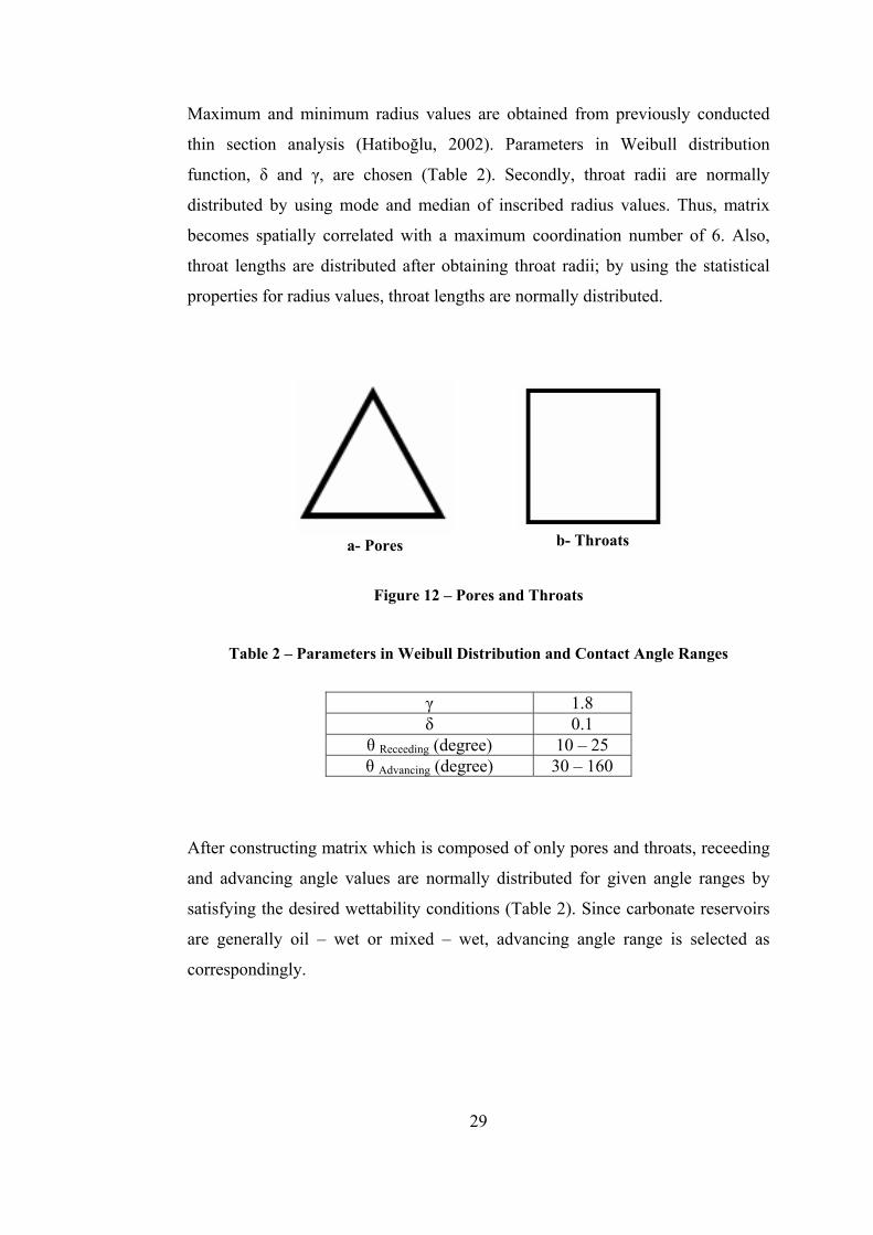
Figure 12 Pores and Throats............................................................................. 29
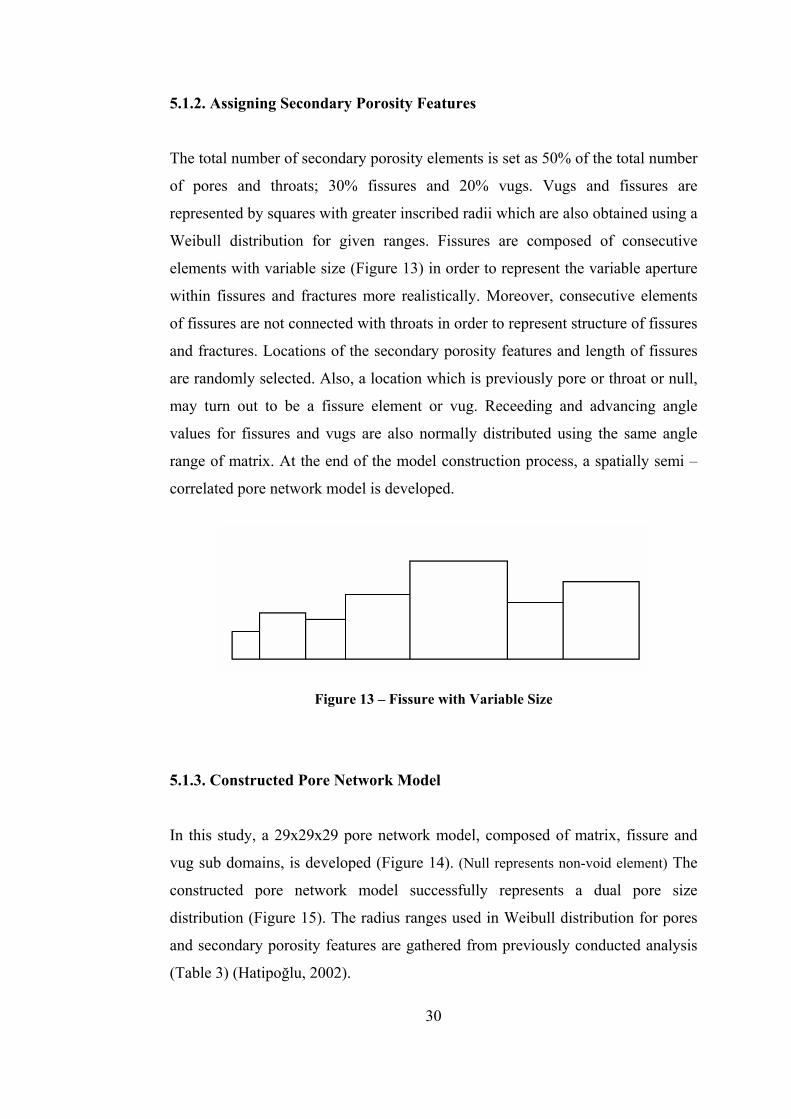
Figure 13 Fissure with Variable Size ............................................................... 30
Figure 14 Distribution of Sub Domains ........................................................... 31
Figure 15 Pore Size Distribution ...................................................................... 31
Figure 16 Phase Area Distribution within Elements ........................................ 37
Figure 17 Phase Area Distribution with Non – Wetting Phase Layer.............. 37
Figure 18 Capillary Pressure Curves for Drainage and Imbibition.................. 41
Figure 19 Relative Permeability Curves (Drainage) ........................................ 42
Figure 20 Relative Permeability Curves (Imbibition)...................................... 42
Figure 21 Comparison of Capillary Pressure Curves with Valvatne (2004) A
(Primary Drainage)........................................................................................... 44
Figure 22 Comparison of Relative Permeability Curves with
Valvatne (2004) B (Primary Drainage) ............................................................ 44
Figure 23 Comparison of Capillary Pressure Curves with
Bekri et al. (2004) (Imbibition) ........................................................................ 45
xv
Figure 24 Comparison of Relative Permeability Curves with Bekri et al. (2004)
(Imbibition) ...................................................................................................... 46
Figure 25 Oil Saturation Distribution (At the end of drainage) ....................... 47
Figure 26 Water Saturation Distribution (At the end of imbibition)................ 48
Figure 27 Relative Permeability Curves for Wettability Analysis
(Primary Drainage)........................................................................................... 50
Figure 28 Relative Permeability Curves for Wettability Analysis
(Waterflooding) ................................................................................................ 50
Figure 29 Preference of Imbibition Mechanisms for Different Wettability
Conditions ........................................................................................................ 51
Figure 30 Preference of In Mechanisms ........................................................... 52
Figure 31 Relative Permeability Curves for Large Sized Element
(Primary Drainage)........................................................................................... 54
Figure 32 Relative Permeability Curves for Large Sized Elements
(Waterflooding) ................................................................................................ 54
Figure 33 Relative Permeability Curves for Small Sized Elements
(Primary Drainage)........................................................................................... 56
Figure 34 Relative Permeability Curves for Small Sized Elements
(Waterflooding) ................................................................................................ 56
Figure 35 Capillary Pressure Curves for Base Model and Matrix (Drainage). 58
Figure 36 Relative Permeability Curves for Vuggy Base Model (Drainage) .. 58
Figure 37 Relative Permeability Curves for Vuggy Base Model
(Waterflooding) ................................................................................................ 59
Figure 38 Relative Permeability Curves for Vuggy Base Model
(Wettability Analysis for Drainage) ................................................................. 60
Figure 39 Relative Permeability Curves for Vuggy Base Model
(Wettability Analysis for Waterflooding) ........................................................ 61
xvi
NOMENCLATURE
A Area, L2
a Random number
bpin Length of water-wet corner, L
D Threshold pressure function
f Boundary condition parameter
F Threshold pressure function
g Conductance, L4
G Dimensionless shape factor
kr Relative permeability
n Number of invaded neighbor elements
nc Number of corners
Num Total number of elements
Pc Capillary pressure, m/Lt2
Pc_max Maximum capillary pressure during primary drainage, m/Lt2
r Radius of curvature, L
R Radius, L
Rn Mean radius of curvature, L
Sw Water saturation, fraction
So Oil saturation, fraction
x Random number
Greek Letters
α Corner half angle, radians
β Angle, radians
γ Weibull distribution function parameter
δ Weibull distribution function parameter
θ Contact angle, radians

xvii
θmax Maximum contact angle for spontaneous imbibition, radians
μ Viscosity, m/Lt
σ Interfacial tension, m/t2
φ1 Conductance function parameter
φ2 Conductance function parameter
φ3 Conductance function parameter
Ω Effective perimeter, L
Subscripts
a Advancing
advancing Advancing
c Corner
center Center
corner Corner
eff Effective
ins Inscribed
Max Maximum
Min Minimum
nw Non-wetting phase
o Oil
p Phase Type (nw or w)
r Receeding
receeding Receeding
t Total (for element)
T Total (for model)
w Wetting phase
1
CHAPTER 1
INTRODUCTION
Studies in reservoir modeling and oil recovery estimation require accurate
prediction of rock and fluid properties, and a good understanding of flow
mechanisms. Properties like relative permeability and wettability have significant
influence on oil recovery and they should be predicted as close to reality as
possible (Honarpour and Mahmood, 1986). Moreover, identification of flow
mechanisms is essential since probable phase entrapments can be determined by
understanding flow in porous media.
Relative permeability curves are generally obtained by steady or unsteady state
experimental methods. Although steady state methods yield accurate and reliable
results, they are time consuming. On the other hand, unsteady state methods are
less time consuming but resulting uncertainties and have operational constraints
like capillary end effects or viscous fingering (Honarpour and Mahmood, 1986).
Moreover, effects of wettability cannot be clearly identified by using experimental
techniques. Thus, in order to obtain relative permeability curves and investigate
effects of wettability, pore network models and pore scale modeling studies are
conducted. Pore network modeling is an effective tool in determination of relative
permeabilities in cases where experimental methods are not sufficient and
successful or heterogeneity in porous media is high.
In early pore scale studies, porous media was represented by sphere packs or
bundle of tubes. Fatt (1956) initiated use of pore network models by proposing a
new model for porous media by combining sphere pack and bundle of tubes
approaches. Later on, studies for homogeneous and isotropic porous media were
2
conducted by using pore networks and flow mechanisms were simulated (Dullien
et al., 1976). After implementation of invasion-percolation theory into pore scale
modeling (Larson et al., 1981; Wilkinson and Willemsen, 1983) and enhances in
pore space extraction methods, it became possible to obtain relative permeability
and capillary pressure curves similar to the experimental results (Heiba et al.,
1983; Oren et al, 1997; Blunt, 1997).
In pore scale studies, it is essential to represent porous media accurately. By using
topologically equivalent pore network models, it is possible to obtain good
matches with simulation and experimental results (Oren et al, 1997). During the
last decade, studies in pore network modeling of sandstones increased. By using
different pore size determination methods, like NMR (Kamath et al., 1998;
Ioannidis and Chatzis, 2000; Moctezuma et al., 2003; Bekri et al., 2004), CT
imaging (Piri, 2003), X-ray tomography, topologically equivalent pore space for
sandstones can be constructed, since porous media is relatively homogeneous and
simple. On the contrary, carbonates have complex and heterogeneous pore space
due to secondary porosity features like vugs, fissures and fractures.
Representation of the complicated flow behavior and determination of wettability
effects within the complex porous media of carbonate rocks, are relatively hard
and require additional techniques (Blunt, 2001). Conventional experimental
methods are inadequate to determine flow properties and to yield precise pore size
distribution of heterogeneous carbonates. Thus, studies in pore network modeling
of carbonates are conducted for granular type carbonates (Valvatne, 2004;
Nguyen et al., 2005). As for heterogeneous vuggy carbonates, pore network
modeling is recently initiated (Kamath et al., 1998; Ioannidis and Chatzis, 2000;
Moctezuma et al., 2003; Bekri et al., 2004; Bekri et al., 2005) and for fractures
and fissured carbonates, studies are limited (Hughes and Blunt, 2001; Wilson-
Lopez and Rodriguez, 2004).
In this study, a pore network model is constructed for simulating two-phase flow
in fissured and vuggy carbonates. In Chapter 2, a literature review on pore
structure of carbonate rocks is provided. In Chapter 3, pore network modeling and

3
flow mechanisms are introduced. The statement of the problem will be presented
and methodology part will follow in Chapter 4 and 5 respectively. Results and
discussion are presented in Chapter 6 and conclusion will be given in Chapter 7.
4
CHAPTER 2
LITERATURE REVIEW
Pore scale modeling is an effective method in determination of wettability effects
on relative permeability and capillary pressure curves. By using topologically
equivalent representation of porous media, flow properties can be predicted
accurately.
Representing porous media and simulating single and multiphase flow at pore
scale are technologically enhancing study areas. During the early stages of
network modeling, sphere of packs and bundle of tubes approaches were used to
represent porous media. Initially, sphere packs were implemented in flow
modeling studies and it was concluded that complex pore geometry in sphere
packs prevented the derivation of flow properties (Fatt, 1956). In bundle of tubes
approach, flow in porous media could be successfully described by relatively
simple mathematical expressions whereas representation of real porous media
might not be accurate. Moreover, bundle of tubes approach was not capable for
elucidating capillary hysteresis and existence of residual saturation wetting or
non-wetting phase saturation (Fatt, 1956; Dullien, 1992). Thus, in order to
determine flow properties and understand flow mechanisms and wettability
effects, Fatt (1956) demonstrated a pioneering approach where use of tube
networks combined with pre-used methods, successfully represented flow
properties.
In this study, a pore network model for fissured and vuggy carbonates is
developed. Since carbonate reservoirs contain more than 60% of world remaining
5
oil in place and 40% of the world gas reserves (SLB, 2008), it is essential to
understand flow mechanisms and wettability effects in carbonate rocks.
2.1 Carbonate Reservoirs
Carbonates are sedimentary rocks deposited in marine environments. Biological in
origin, carbonates are composed of fragments of marine organisms, skeletons,
coral, algae and precipitated mostly calcium carbonate. They are chemically
active and easily altered. The deposition area directly affects the heterogeneity of
carbonate grains. Once carbonate rock is formed, a range of chemical and physical
processes begins to alter the rock structure changing fundamental characteristics
such as porosity and permeability.
At deposition, carbonate sediments often have very high porosities (35%–75%)
but this decreases sharply as the sediment is altered and buried to reservoir depths.
As a result, carbonate reservoirs exhibit abrupt variations in rock type distribution
(SLB, 2008). Thus, a complex porous media and heterogeneous pore network are
present within carbonate rocks and carbonate reservoirs are generally
characterized by extreme heterogeneity of porosity and permeability. They can be
massive, vuggy and fractured in the organic reef facies or highly stratified, often
vertically discontinuous in the back reef and shoal facies (Jardine et al., 1977).
Contrary to sandstones, carbonate reservoirs are generally mixed – wet or oil –
wet (SLB, 2008).
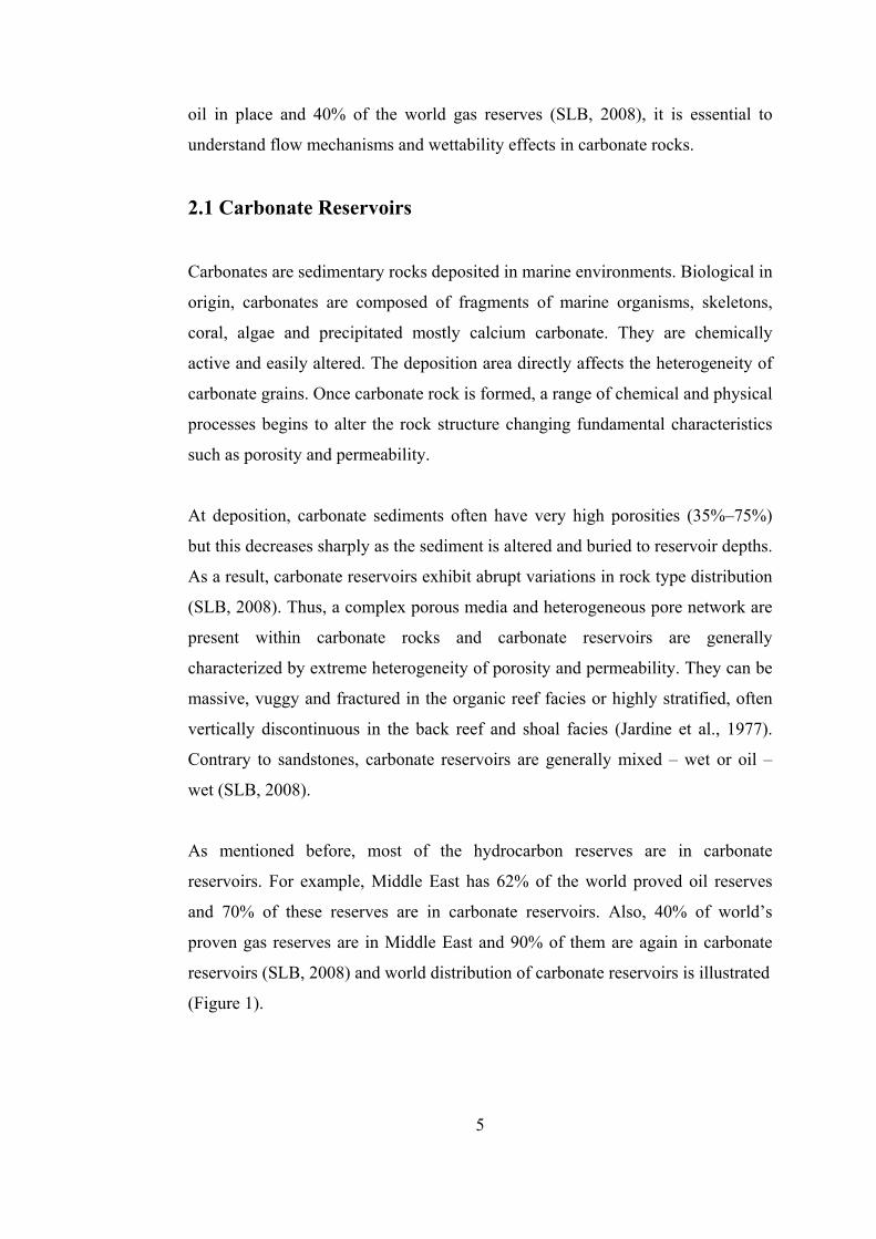
As mentioned before, most of the hydrocarbon reserves are in carbonate
reservoirs. For example, Middle East has 62% of the world proved oil reserves
and 70% of these reserves are in carbonate reservoirs. Also, 40% of world’s
proven gas reserves are in Middle East and 90% of them are again in carbonate
reservoirs (SLB, 2008) and world distribution of carbonate reservoirs is illustrated
(Figure 1).
6
Despite the difficulties in characterizing and identifying, it is essential to
understand flow behavior in carbonate reservoir in order to forecasting production
accurately.
Figure 1- World Distribution of Carbonate Reservoirs (SLB, 2008)
2.2 Pore Structure of Carbonates
2.2.1. Porosity Types in Carbonates
Several mechanisms influence porosity evolution and pore-size distribution in
carbonate rocks. Mainly, there are two types of porosity; primary interparticle and
secondary. Primary interparticle porosity is formed by deposition of calcareous
sand or gravel under the influence of strong currents or waves or by local
production of calcareous sand-size particles with sufficient rapidity to deposit
particle on particle with little or no interstitial mud. Secondary porosity is formed
by dissolution of interstitial mud in calcareous sand and the result is microvuggy
porosity resembling inter particle pore space.
7
2.2.1.1. Primary Porosity
Primary porosity includes pore types which result from depositional processes and
which have been modified slightly by compaction, pressure solution, and simple
pore filling cement, or dissolution alteration.
According to Murray (1960), primary porosity is originated from framework, mud
and sands. Framework material could be organic or inorganic and commonly
composed of tightly interlocking crystals of calcite or aragonite. Mud consists of
particles that are chemically or biochemically precipitated fine crystals or finely
comminuted debris of larger particles. In addition, carbonates can be deposited as
sands, which are generally deposited under conditions of sufficiently rapid water
movement either to remove the finer particles or to transport and selectively
deposit larger particles.
Primary pore types can be destroyed; porosity and pore size may be reduced either
by cementation or by cementation in conjunction with replacement. Commonly
observed cementing materials are calcite, anhydrite, and quartz. Calcite cement
appears to be especially common where the particles are monocrystalline (Moore,
2001).
2.2.1.2. Secondary Porosity
Secondary porosity in carbonates is composed of different features like vugs,
fractures and fissures. As mentioned before, in early stages of diagenesis,
carbonates are composed of framework material and during diagenesis vugs are
formed generally within the framework. Fracture and fissures may be formed by
post depositional processes. Their geometry and intensity are dependent on
several factors like geomechanical and lithological properties (Peacock and Mann,
2005).
8
Secondary vugs are void spaces formed by post-depositional processes. Vugs are
larger than the simple fitting together of associated mutually interfering crystals or
deposited particles. Several mechanisms involve in formation of vugs;
replacement of anhydrite, carbonate dissolution, replacement of dolomite and
fracturing (Mazullo, 2004).
Fractures have an important role in porosity of carbonate rocks. The style,
geometry and distribution of fractures can be controlled by various factors; such
as, rock characteristics and diagenesis (lithology, sedimentary structures, bed
thickness, mechanical stratigraphy, the mechanics of bedding planes); structural
geology (tectonic setting, paleostresses, subsidence and uplift history, proximity
to faults, position in a fold, timing of structural events, mineralization, the angle
between bedding and fractures); and present-day factors; such as, orientations of
in situ stresses, fluid pressure, perturbation of in situ stresses and depth (Peacock
and Mann, 2005). Furthermore, lithological competence can control the geometry
and distribution of fractures, with more fractures tending to occur in more brittle
beds. Sedimentary structure can be considered as weakness points and fractures
can initiate at such anisotropies as bedding plane irregularities and fossils.
Moreover, bed thickness affects spacing of joint sets within a bed. It is commonly
approximately proportional to bed thickness, with joint frequencies tending to be
higher in thinner beds than in thicker beds. Also, mechanical behavior of the
bedding planes can control fracture propagation and mechanical stratigraphy
(Peacock and Mann, 2005).
2.2.2. Porosity Classification of Carbonate Rocks
Porosity classification of carbonate rocks is different and more difficult than the
classification in siliciclastic rocks. Since carbonates are composed of fragmental
or non-fragmental particles, micrite or sparry calcite cements and may involve
fractures, vugs or fissures; their porosity classification requires additional care.
Thus, many carbonate sedimentologists propose different porosity classification
9
methods, generally based on rock fabric, petrophysical properties, modifying
terms and timing.
The pore types can be generally classified as intergrain/intercrystal,
moldic/intrafossil/shelter and cavernous/fracture/solution enlarged fracture. This
general classification was further divided according to visibility and rock fabric
related to petrophysical properties by Archie (1952), rock fabric and petrophysical
properties by Lucia (1983) (further improvements in 1995 and 1999) and fabric
selectivity by Choquette and Pray (1970).
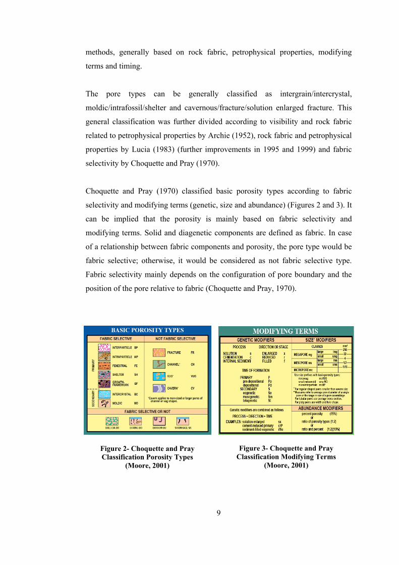
Choquette and Pray (1970) classified basic porosity types according to fabric
selectivity and modifying terms (genetic, size and abundance) (Figures 2 and 3). It
can be implied that the porosity is mainly based on fabric selectivity and
modifying terms. Solid and diagenetic components are defined as fabric. In case
of a relationship between fabric components and porosity, the pore type would be
fabric selective; otherwise, it would be considered as not fabric selective type.
Fabric selectivity mainly depends on the configuration of pore boundary and the
position of the pore relative to fabric (Choquette and Pray, 1970).
Figure 2- Choquette and Pray Classification Porosity Types
(Moore, 2001)
Figure 3- Choquette and Pray
Classification Modifying Terms (Moore, 2001)
10
For primary porosity (syndepositional porosity), fabric selectivity is totally
determined by fabric components; where as in secondary porosity, which is
formed after final deposition, fabric selectivity depends on the diagenetic history.
Moreover, Choquette and Pray generated their classification also on genetic and
size modifiers. Genetic modifiers are used for giving more detailed information
about the evolution of porosity and size modifiers are used for expressing the size
of the pores.
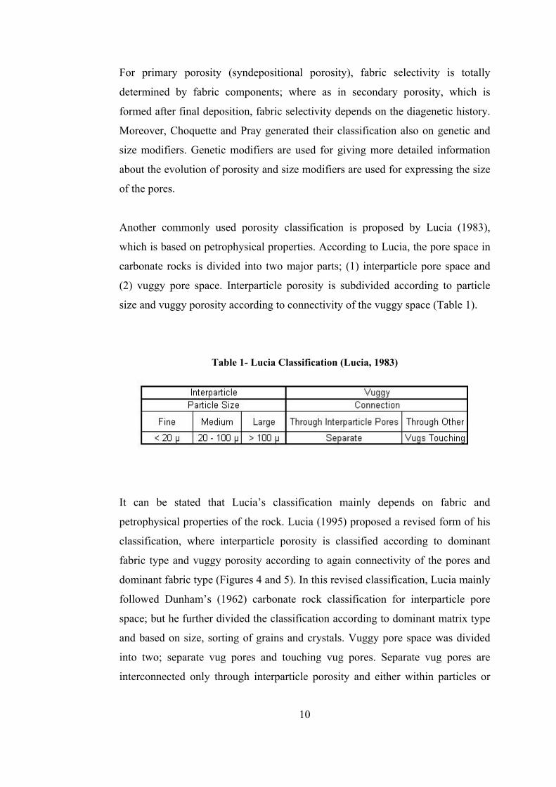
Another commonly used porosity classification is proposed by Lucia (1983),
which is based on petrophysical properties. According to Lucia, the pore space in
carbonate rocks is divided into two major parts; (1) interparticle pore space and
(2) vuggy pore space. Interparticle porosity is subdivided according to particle
size and vuggy porosity according to connectivity of the vuggy space (Table 1).
Table 1- Lucia Classification (Lucia, 1983)
It can be stated that Lucia’s classification mainly depends on fabric and
petrophysical properties of the rock. Lucia (1995) proposed a revised form of his
classification, where interparticle porosity is classified according to dominant
fabric type and vuggy porosity according to again connectivity of the pores and
dominant fabric type (Figures 4 and 5). In this revised classification, Lucia mainly
followed Dunham’s (1962) carbonate rock classification for interparticle pore
space; but he further divided the classification according to dominant matrix type
and based on size, sorting of grains and crystals. Vuggy pore space was divided
into two; separate vug pores and touching vug pores. Separate vug pores are
interconnected only through interparticle porosity and either within particles or
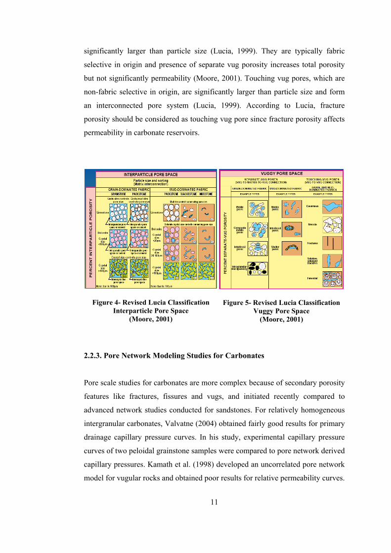
11
significantly larger than particle size (Lucia, 1999). They are typically fabric
selective in origin and presence of separate vug porosity increases total porosity
but not significantly permeability (Moore, 2001). Touching vug pores, which are
non-fabric selective in origin, are significantly larger than particle size and form
an interconnected pore system (Lucia, 1999). According to Lucia, fracture
porosity should be considered as touching vug pore since fracture porosity affects
permeability in carbonate reservoirs.
Figure 4- Revised Lucia Classification
Interparticle Pore Space (Moore, 2001)
Figure 5- Revised Lucia Classification
Vuggy Pore Space (Moore, 2001)
2.2.3. Pore Network Modeling Studies for Carbonates
Pore scale studies for carbonates are more complex because of secondary porosity
features like fractures, fissures and vugs, and initiated recently compared to
advanced network studies conducted for sandstones. For relatively homogeneous
intergranular carbonates, Valvatne (2004) obtained fairly good results for primary
drainage capillary pressure curves. In his study, experimental capillary pressure
curves of two peloidal grainstone samples were compared to pore network derived
capillary pressures. Kamath et al. (1998) developed an uncorrelated pore network
model for vugular rocks and obtained poor results for relative permeability curves.
12
Ioannidis and Chatzis (2000) proposed a dual network model for representation of
pore structure for vuggy carbonates. They constructed a dual porosity network
model by combining X-ray and CT analysis results. Vugs were superimposed on
matrix blocks in an agreement with porosity distribution of the sample.
Moctezuma et al. (2003) constructed a dual network model, composed of matrix,
vugs and fractures combining vugs, for a vuggy carbonate. The equivalent pore
network model was developed by combining mercury invasion data and NMR
measurements. Bekri and Laroche (2004) extended Moctezuma’s study to
investigate wettability effects on vuggy carbonates and, calculate transport and
electrical properties (2005). By constructing a 3-D pore network model, capillary
pressure and relative permeability curves were determined which were in
agreement with the experimental data. Okabe (2004) and Al-Kharusi (2007)
extracted pore space from CT images for carbonates and developed a pore scale
simulator for determining flow properties.
As for fractures, microfractures and fissures, Hughes and Blunt (2001) simulated
multiphase flow in a single fracture represented by square lattices connected by
throats and extended this study to investigate matrix/fracture transfer (2001). For
modeling two-phase flow in microfractured porous media, a network model
composed of pores, without throats, with variable cross sections was used by
Wilson-Lopez and Rodriguez (2004). A recent study is conducted by Erzeybek
and Akın (2008) for modeling two – phase flow in fissured and vuggy carbonates.
Both fissures and vugs are implemented into pore network and various properties
like wettability and pore morphology are examined.
2.3 Advanced Studies in Pore Network Modeling
Technological improvements in computer science and advanced imaging tools
like CT and SEM yield enhancements in pore scale modeling. Pore scale studies
can be coupled with neural networks to simulate flow in porous media (Karaman,
2002). In addition, use of pore network models is extended to other research areas
13
such as modeling miscible CO2 flooding (Uzun, 2005) and flow of Non-
Newtonian fluids or NAPLs. In hydrology, pore scale modeling can be used for
identification of NAPL behavior within the porous media. Non-Newtonian fluids
used in petroleum industry are polymeric solutions with shear-thinning behavior,
unlike Newtonian fluids which are conventionally found in reservoirs. Since it is
hard to determine relative permeability and capillary pressure curves of NAPLs
and Non-Newtonian fluids by experiments, pore network modeling studies can be
used for obtaining flow properties for those kinds of fluids.
Jia et al. (1999) conducted visualization experiments and numerical simulations in
pore networks for understanding basic aspects of mass transfer during the
solubilization of residual non-aqueous phase liquids NAPL. Moreover, Al-Futaisi
and Patzek (2004) studied spontaneous and forced secondary imbibition of NAPL
invaded sediment by using a 3-D uncorrelated pore network model of a mixed-wet
soil.
For simulating Non-Newtonian flow in porous media, studies are recently
conducted (Lopez et al., 2003; Balhoff, 2005; Sochi, 2007). Lopez et al. (2003)
studied the flow of power law fluids in porous media at pore scale. By using an
accurate representation of pore space and bulk rheology (variation of viscosity
with shear rate), a relationship between pressure drop and average flow velocity in
each pore was defined. They predicted the experimental results successfully but
their study was limited to simple shear-thinning fluids. Balhoff (2005) reported
pore scale modeling of Non-Newtonian fluids. He used an unconsolidated porous
media to simulate flow of polymers and suspensions. He predicted flow properties
for steady state flows. Also, viscous fingering patterns of Non-Newtonian fluids
were examined during transient displacement.
Sochi (2007) constructed a topologically disordered pore network model and
simulated flow of Non-Newtonian fluids. Pressure field was obtained iteratively
and volumetric flow rate and apparent viscosity values were determined.
Moreover, time-independent category of the non-Newtonian fluids is investigated
14
using two time-independent fluid models and a comparison between the model
and the experimental results was carried out. The yield-stress phenomenon was
also investigated and several numerical algorithms were developed and
implemented to predict threshold yield pressure of the network.
Apart from the studies conducted for Non-Newtonian fluid and NAPLs, pore scale
modeling is used for construction of sedimentary rocks and mechanical properties
(Bakke and Oren, 1997; Jin and Patzek, 2003). Bakke and Oren (1997) developed
a pore network model by simulating the main sandstone forming geological
processes. They successfully modeled sand grain sedimentation, cementation and
diagenesis by using the input data gathered from thin section analysis and
obtained a topologically equivalent representation of porous media.
Jin and Patzek (2003) developed a depositional model by constructing geometrical
structure and mechanical properties of sedimentary rocks. They obtained two and
three-dimensional porous media for unconsolidated sand and sandstones. At pore
scale, they simulated the dynamic geologic processes of grain sedimentation,
compaction and diagenetic rock transformations and obtained mechanical
properties. Moreover, the depositional model was used for studying initiation,
growth and coalescence of micro-cracks.
Pore network modeling can also be used for modeling advanced processes such as
in-situ combustion (Lu and Yortsos, 2001) or coal structure modeling (Tomeczek
and Mlonka, 1998). Lu and Yortsos (2001) used a pore network model composed
of pores and solid sites, for modeling the effect of the microstructure on
combustion processes in porous media. In the model, flow and transport of the gas
phase occurred in the pore space with convection, whereas heat transfer occurred
in solid phase by conduction. Tomeczek and Mlonka (1998) represented coal with
both cylindrical and non-cylindrical pores. By using the experimental porosity,
they concluded that not only cylindrical pores but also non-cylindrical, spherical
pores contributed. They modified a previously developed random pore model by
implementing spherical vesicles.
15
CHAPTER 3
PORE NETWORK MODELING
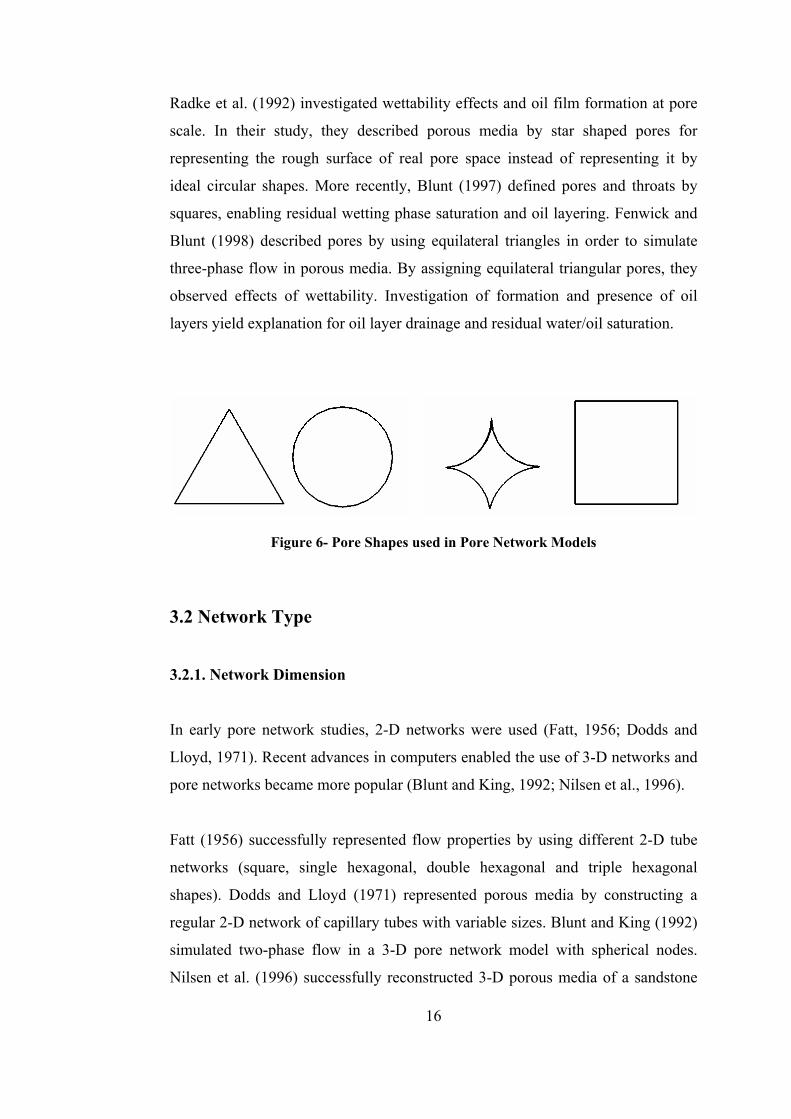
3.1. Pore Morphology
In early pore network studies, porous media is described by pores and throats that
have circular cross sections or by spheres (Blunt and King, 1992). Applying flow
equations and solving mathematical expressions for simple circular cross sections
are relatively less time consuming. In circular pores, only one phase can be
present and thus, effects of wettability cannot be determined accurately.
Moreover, circular cross section does not reflect the real porous space. Therefore,
different types of pores are needed in pore networks. That’s why pore types with
equilateral or irregular triangular, square and star shaped cross sections are
generally used for description of porous media (Figure 6) (Oren et al., 1997;
Blunt, 1997; Radke et al., 1992; Hui and Blunt, 2000; Valvatne and Blunt, 2003;
Patzek, 2000). In recent studies (Patzek and Silin, 2001; Piri and Blunt, 2005),
porous media is represented by combination of triangular, circular or square cross-
sections.
Blunt and King (1992) simulated two phase flow at pore scale by constructing a
pore network consisted of pores and throats with spherical geometry. Oren et al.
(1997) described pore space by cylindrical shapes with different dimensionless
shape factors. By assigning various shape factors, irregular porous media was
represented by topologically equivalent irregular triangles. Thus, irregularity in
real porous media was reflected and effects of wettability could be observed.
16
Radke et al. (1992) investigated wettability effects and oil film formation at pore
scale. In their study, they described porous media by star shaped pores for
representing the rough surface of real pore space instead of representing it by
ideal circular shapes. More recently, Blunt (1997) defined pores and throats by
squares, enabling residual wetting phase saturation and oil layering. Fenwick and
Blunt (1998) described pores by using equilateral triangles in order to simulate
three-phase flow in porous media. By assigning equilateral triangular pores, they
observed effects of wettability. Investigation of formation and presence of oil
layers yield explanation for oil layer drainage and residual water/oil saturation.
Figure 6- Pore Shapes used in Pore Network Models
3.2 Network Type
3.2.1. Network Dimension
In early pore network studies, 2-D networks were used (Fatt, 1956; Dodds and
Lloyd, 1971). Recent advances in computers enabled the use of 3-D networks and
pore networks became more popular (Blunt and King, 1992; Nilsen et al., 1996).
Fatt (1956) successfully represented flow properties by using different 2-D tube
networks (square, single hexagonal, double hexagonal and triple hexagonal
shapes). Dodds and Lloyd (1971) represented porous media by constructing a
regular 2-D network of capillary tubes with variable sizes. Blunt and King (1992)
simulated two-phase flow in a 3-D pore network model with spherical nodes.
Nilsen et al. (1996) successfully reconstructed 3-D porous media of a sandstone
17
sample reconstructed by using thin section analysis and numerical modeling of
main geological processes.
3.2.2. Flow Behavior
In pore scale studies, mainly two types of model are used: quasi-static and
dynamic. Quasi-static models involve use of invasion percolation process and
capillary forces are dominant. On the other hand, dynamic models require an input
flow rate and both capillary and dynamic forces are considered.
3.2.2.1. Quasi-Static Network Models
Fluid flow is dominated either by capillary or viscous forces alone or both. In
quasi-static flow, capillary force is the driving force. Thus effects of dynamic
aspects are neglected. Final static position of fluid interfaces and configurations
are determined in quasi-static networks. Interfacial forces are dominant since
capillary number is small (Jia, 2005).
In quasi-static network modeling, invasion-percolation process is implemented for
simulating flow in reconstructed porous media. Invasion-percolation process is
based on percolation theory (Wilkinson and Willemsen, 1983). Initially,
percolation theory is used for describing morphology, conductivity and flow at
pore scale (Larson et al., 1981). Percolation process is defined by the fluid flow
path determined by the porous media, which is random (Larson et al., 1981). Later
on, Wilkinson and Willemsen (1983) defined invasion-percolation describing
dynamically flow processes by using constant rate rather than constant applied
pressure at pore scale.
3.2.2.2. Dynamic Network Models
Dynamic network models can be used for investigating the effects of both
interfacial and viscous forces. In this kind of network model, a certain flow rate is
18
imposed on network and pressure field is calculated iteratively. Configurations of
elements are transiently determined. Since both interfacial and viscous forces are
implemented in dynamic network models, the preference between viscous and
interfacial forces depends on the capillary number. For low values of capillary
number, interfacial forces are dominant whereas for higher values viscous forces
are effective. Contrary to quasi-static ones, dynamic networks are not limited to
low capillary numbers. Thus, effects of displacement rate on imbibition can be
determined easily by using dynamic network models (Jia, 2005).
Dynamic network models are used for investigating flow rate and wettability
effects on relative permeability and capillary pressure curves (Koplick and
Lasseter, 1985; Dias and Payatakes, 1986a; Lenormand et al., 1988; Mogensen
and Stenby, 1998; Hughes and Blunt, 2000; Nguyen et al., 2005). Koplick and
Lasseter’s (1985) study was the first of its kind where a dynamic model was
developed for pore scale modeling. By assuming equal viscosities, 2-phase flow
was simulated in porous media which was represented by spherical pores and
cylindrical throats. Lenormand et al. (1988) constructed a dynamic model for
simulating pore scale immiscible displacement by using a two dimensional porous
media constructed by interconnected capillaries. In order to study the effects of
viscous and capillary forces on relative permeability, Blunt and King (1992)
developed 2-D and 3-D two-phase dynamic models.
Mogensen and Stenby (1998) constructed a 3-D dynamic pore network model for
investigating imbibition processes. They observed the effects of contact angle,
aspect ratio and capillary number on the competition between piston-like advance
and snap-off mechanisms during imbibition. Hughes and Blunt (2000) also
constructed a dynamic pore network to study the effects of flow rate and contact
angle on relative permeability. They were successful at identifying displacement
patterns throughout the imbibition process by varying capillary number, contact
angle and initial wetting phase saturation. More recently, Nguyen et al. (2005)
developed a dynamic pore network model representing flow in Berea sandstone.
They investigated the effects of displacement rate and wettability on imbibition
19
relative permeability. They recognized the inhibiting effect of displacement rate
on snap-off during imbibition.
3.2.3. Spatially Correlated and Uncorrelated Networks
In pore scale studies, there are two main methods used in characterization of
porous media: tuning geometric parameters of a regular network model and
modeling the random topology of pore space directly. In the first method, a
regular network model, which is spatially correlated, is used and corresponding
geometric parameters are tuned to match experimental data. Although this method
yields more accurate results than simple correlations, predictions are still poor. In
the second method, porous media is directly constructed by using only pore size
distribution data gathered from thin section analysis. Then, sedimentation and
compaction are simulated and a random pore network is obtained. This approach
results accurate prediction for sedimentary structures but statistical methods are
required for carbonate rocks (Blunt, 2001). In reconstructed pore networks, spatial
correlation and connectivity are directly incorporated in the model (Blunt, 2001).
Two approaches are mainly used in representing spatial correlation in porous
media: short-range correlations like spherical, Gaussian and exponential structures
and long-range correlations like fractal concepts (Mani and Mohanty, 1999).
Besides pore size distribution and pore – throat aspect ratio, spatial correlation has
also an influence on flow properties. Mani and Mohanty (1999) studied the effects
of spatial correlations on multiphase phase flow properties. They observed similar
trends in primary drainage and imbibition characteristics for spatially uncorrelated
and correlated porous media. Realization independent absolute permeability and
capillary pressure curves were obtained. For spatial correlations represented by
long-range correlations, realization dependent capillary pressure curves were
reported. Also, effects of spatial correlation on primary drainage and imbibition
capillary pressure curves were observed. In spatially correlated networks, primary
drainage capillary pressure curves were more gradual with respect to the ones in
uncorrelated networks. Moreover, higher wetting and non – wetting phase relative
20
permeability values were obtained during primary drainage as spatial correlation
increased. As for imbibition, they reported increase in probability for snap – off
and decrease in probability for piston – like advance in spatially correlated
systems (detailed information about the processes is presented in Section
3.3).Thus, higher residual non – wetting phase saturation at the end of imbibition
were observed as spatial correlation increased. Steeper imbibition capillary
pressure curves were obtained for correlated networks with respect to uncorrelated
ones (Mani and Mohanty, 1999).
Pore networks are generally assumed to be spatially uncorrelated but it is reported
that spatial correlation yields more accurate results with limited predictive
capabilities. Thus, Knackstedt et al. (2001) introduced correlated heterogeneity
and investigated its effects on two – phase flow properties. They reported
significant effect of small-scale correlations on the structure of fluid clusters at
breakthrough and at the residual saturation. Also, lower residual phase saturations
were observed in correlated heterogeneous pore networks than in the random
ones. They concluded that correlated heterogeneity has a strong influence on the
final configuration of trapped fluid clusters.
3.3 Flow Mechanisms
In porous media, fluid flow occurs by different mechanisms mainly; snap-off,
piston-like advance and pore-body filling. In primary drainage, the elements are
assumed to be filled by piston-like advance. On the other hand, during imbibition
(for example waterflooding) process, the competition between the flow
mechanisms is considered. The detailed descriptions for the mechanisms are
provided respectively.
3.3.1. Snap – Off
Snap-off is the invasion by wetting-phase arc menisci present in the corners of an
element. The arc menisci displaces the non-wetting phase present in the center
21
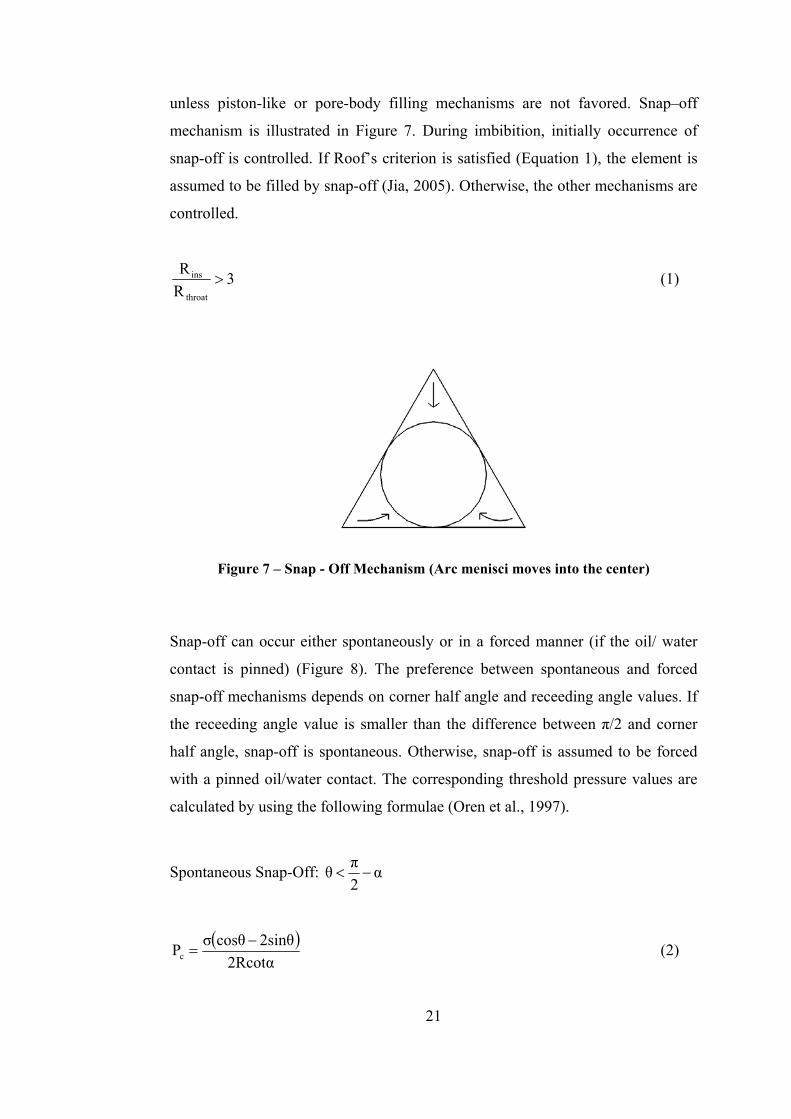
unless piston-like or pore-body filling mechanisms are not favored. Snap–off
mechanism is illustrated in Figure 7. During imbibition, initially occurrence of
snap-off is controlled. If Roof’s criterion is satisfied (Equation 1), the element is
assumed to be filled by snap-off (Jia, 2005). Otherwise, the other mechanisms are
controlled.
3RR
throat
ins > (1)
Figure 7 – Snap - Off Mechanism (Arc menisci moves into the center) Snap-off can occur either spontaneously or in a forced manner (if the oil/ water
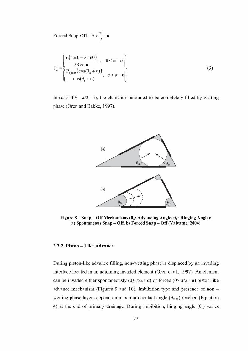
contact is pinned) (Figure 8). The preference between spontaneous and forced
snap-off mechanisms depends on corner half angle and receeding angle values. If
the receeding angle value is smaller than the difference between π/2 and corner
half angle, snap-off is spontaneous. Otherwise, snap-off is assumed to be forced
with a pinned oil/water contact. The corresponding threshold pressure values are
calculated by using the following formulae (Oren et al., 1997).
Spontaneous Snap-Off: α2πθ −<
( )2Rcotα
2sinθcosθσPc−
= (2)
22
Forced Snap-Off: α2πθ −>
( )
( )⎪⎪⎭
⎪⎪⎬
⎫
⎪⎪⎩
⎪⎪⎨
⎧
−>+
+
−≤−
=απθ ,
α)cos(θα)cos(θP
απθ , 2Rcotα
2sinθcosθσ
P
r
ac_maxc (3)
In case of θ= π/2 – α, the element is assumed to be completely filled by wetting
phase (Oren and Bakke, 1997).
Figure 8 – Snap – Off Mechanisms (θa: Advancing Angle, θh: Hinging Angle): a) Spontaneous Snap – Off, b) Forced Snap – Off (Valvatne, 2004)
3.3.2. Piston – Like Advance
During piston-like advance filling, non-wetting phase is displaced by an invading
interface located in an adjoining invaded element (Oren et al., 1997). An element
can be invaded either spontaneously (θ≤ π/2+ α) or forced (θ> π/2+ α) piston like
advance mechanism (Figures 9 and 10). Imbibition type and presence of non –
wetting phase layers depend on maximum contact angle (θmax) reached (Equation
4) at the end of primary drainage. During imbibition, hinging angle (θh) varies
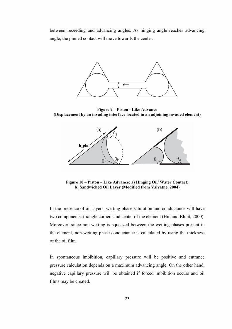
23
between receeding and advancing angles. As hinging angle reaches advancing
angle, the pinned contact will move towards the center.
Figure 9 – Piston - Like Advance (Displacement by an invading interface located in an adjoining invaded element)
Figure 10 – Piston – Like Advance: a) Hinging Oil/ Water Contact; b) Sandwiched Oil Layer (Modified from Valvatne, 2004)
In the presence of oil layers, wetting phase saturation and conductance will have
two components: triangle corners and center of the element (Hui and Blunt, 2000).
Moreover, since non-wetting is squeezed between the wetting phases present in
the element, non-wetting phase conductance is calculated by using the thickness
of the oil film.
In spontaneous imbibition, capillary pressure will be positive and entrance
pressure calculation depends on a maximum advancing angle. On the other hand,
negative capillary pressure will be obtained if forced imbibition occurs and oil
films may be created.
24
⎟⎟⎟⎟
⎠
⎞
⎜⎜⎜⎜
⎝
⎛
+−
+−−=
)θcos(αcosασ
RP)sinαθsin(α1cosθ
rc_max
rmax (4)
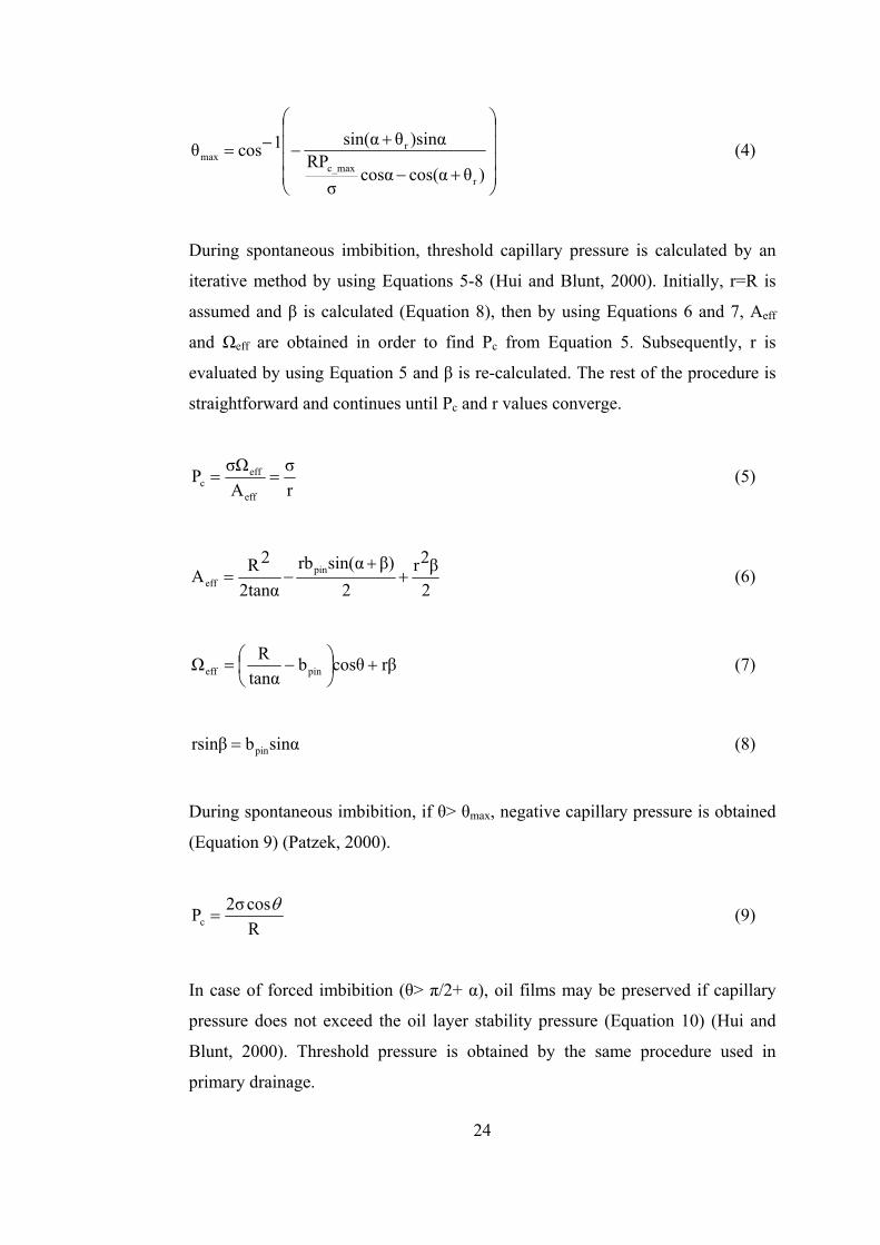
During spontaneous imbibition, threshold capillary pressure is calculated by an
iterative method by using Equations 5-8 (Hui and Blunt, 2000). Initially, r=R is
assumed and β is calculated (Equation 8), then by using Equations 6 and 7, Aeff
and Ωeff are obtained in order to find Pc from Equation 5. Subsequently, r is
evaluated by using Equation 5 and β is re-calculated. The rest of the procedure is
straightforward and continues until Pc and r values converge.
rσ
AσΩP
eff
effc == (5)
2β2r
2β)sin(αrb
2tanα
2RA pineff +
+−= (6)
rβcosθbtanα
RΩ pineff +⎟⎠⎞
⎜⎝⎛ −= (7)
sinαbrsinβ pin= (8)
During spontaneous imbibition, if θ> θmax, negative capillary pressure is obtained
(Equation 9) (Patzek, 2000).
Rcos2σPc
θ= (9)
In case of forced imbibition (θ> π/2+ α), oil films may be preserved if capillary
pressure does not exceed the oil layer stability pressure (Equation 10) (Hui and
Blunt, 2000). Threshold pressure is obtained by the same procedure used in
primary drainage.
25
( )
⎟⎠⎞⎜
⎝⎛ ++
⎟⎟⎠
⎞⎜⎜⎝
⎛⎟⎠⎞
⎜⎝⎛ −−⋅++
=θθαα
θαθααθααασ
2coscossin42sin3b
cossin42cos32cos42sincossin2sincosP
pin
stab
(10)
3.3.3. Pore – Body Filling
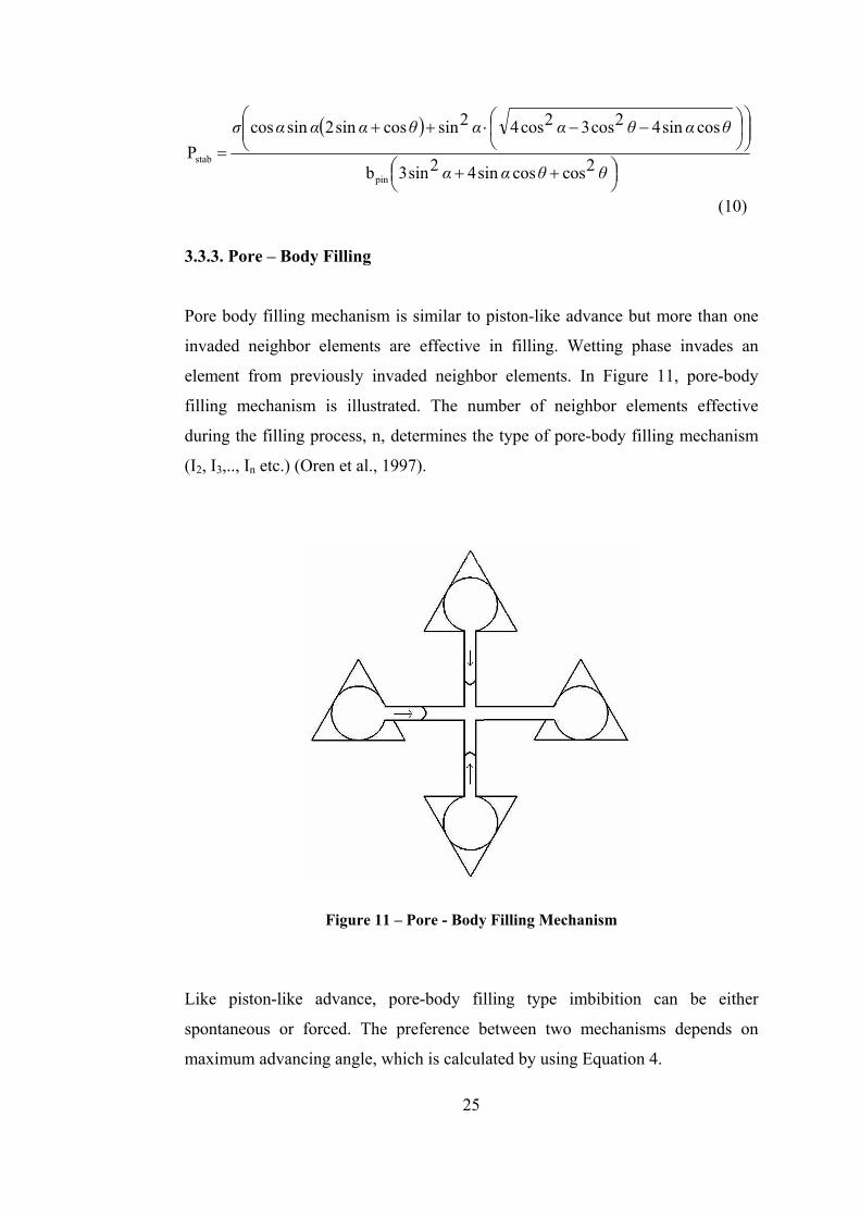
Pore body filling mechanism is similar to piston-like advance but more than one
invaded neighbor elements are effective in filling. Wetting phase invades an
element from previously invaded neighbor elements. In Figure 11, pore-body
filling mechanism is illustrated. The number of neighbor elements effective
during the filling process, n, determines the type of pore-body filling mechanism
(I2, I3,.., In etc.) (Oren et al., 1997).
Figure 11 – Pore - Body Filling Mechanism Like piston-like advance, pore-body filling type imbibition can be either
spontaneous or forced. The preference between two mechanisms depends on
maximum advancing angle, which is calculated by using Equation 4.
26
In spontaneous pore-body filling (in other words if θ≤θmax) threshold pressure of
an element is a function of number of previously invaded neighbor elements and
can be calculated by using the following equations (Oren et al., 1997, Patzek,
2000);
⎟⎟⎠
⎞⎜⎜⎝
⎛∑=
+=n
1ixRaR
cosθ1R iins_iiinsn (11)
nnc, R
2σP = (12)
If only one of the neighbor elements is invaded (n=1), then the mechanism is
similar to piston-like advance and threshold pressure is calculated by using the
same procedure in piston-like advance. If imbibition is forced, then the threshold
pressure is obtained by the same procedure for primary drainage with advancing
angle.
27
CHAPTER 4
STATEMENT OF THE PROBLEM
Carbonates have relatively heterogeneous and complex porous media because of
secondary porosity features like fractures, fissures and vugs. The heterogeneous
structure of carbonate rocks results difficulties in identification of complex flow
mechanisms and determination of flow properties. In pore scale studies
topologically equivalent networks yield accurate representation of flow properties.
However, it is challenging to represent heterogeneous carbonates accurately and
implement a topologically equivalent pore network model for carbonate rocks.
Besides its heterogeneous pore structure, carbonate rocks can be mixed wet,
resulting heterogeneity also in wettability conditions. Due to their complex pore
structure and wettability characteristics, pore scale studies for carbonate rocks are
limited.
In this study, a novel pore network model that simulates two-phase flow in
fissured and vuggy carbonates is developed. Secondary porosity features are
assigned and flow properties within the complex porous media are predicted using
this model. Capillary pressure and relative permeability curves for primary
drainage and waterflooding mechanisms are obtained. Moreover, by assigning
variable contact angle ranges, effects of wettability are observed and mixed wet
conditions are simulated straightforwardly.
28
CHAPTER 5
METHODOLOGY
In this study, a 3-D novel pore network model is developed for simulating two-
phase flow in fissured and vuggy carbonate rock. Initially matrix, which is
composed of pore and throats, is constructed. The corresponding receeding and
advancing angle values are assigned by using normal distribution within a given
range for the corresponding wettability conditions. Following that, secondary
porosity features (fissures and vugs) are assigned in the model. The elements are
constructed for given size ranges, which are obtained from previously conducted
thin section analysis and experimental results. Then, capillary pressure and
relative permeability curves are obtained for primary drainage and waterflooding
mechanisms.
5.1. Construction of Pore Network Model
5.1.1. Assigning Matrix Properties
Matrix is composed of equilateral triangular pores and square throats (Figure 12a-
b). First, inscribed radius values are assigned for pores by using Weibull
distribution (Equation 13) for given radius ranges (Hui and Blunt, 2000).
( ) MinMinMaxins R1/γ
1/δe1/δe1xδlnRRR +⎟⎠⎞
⎜⎝⎛
⎥⎦⎤
⎢⎣⎡ −+⎟
⎠⎞⎜
⎝⎛ −−−−= (13)
29
Maximum and minimum radius values are obtained from previously conducted
thin section analysis (Hatiboğlu, 2002). Parameters in Weibull distribution
function, δ and γ, are chosen (Table 2). Secondly, throat radii are normally
distributed by using mode and median of inscribed radius values. Thus, matrix
becomes spatially correlated with a maximum coordination number of 6. Also,
throat lengths are distributed after obtaining throat radii; by using the statistical
properties for radius values, throat lengths are normally distributed.
a- Pores
b- Throats
Figure 12 – Pores and Throats
Table 2 – Parameters in Weibull Distribution and Contact Angle Ranges
γ 1.8 δ 0.1
θ Receeding (degree) 10 – 25 θ Advancing (degree) 30 – 160
After constructing matrix which is composed of only pores and throats, receeding
and advancing angle values are normally distributed for given angle ranges by
satisfying the desired wettability conditions (Table 2). Since carbonate reservoirs
are generally oil – wet or mixed – wet, advancing angle range is selected as
correspondingly.
30
5.1.2. Assigning Secondary Porosity Features
The total number of secondary porosity elements is set as 50% of the total number
of pores and throats; 30% fissures and 20% vugs. Vugs and fissures are
represented by squares with greater inscribed radii which are also obtained using a
Weibull distribution for given ranges. Fissures are composed of consecutive
elements with variable size (Figure 13) in order to represent the variable aperture
within fissures and fractures more realistically. Moreover, consecutive elements
of fissures are not connected with throats in order to represent structure of fissures
and fractures. Locations of the secondary porosity features and length of fissures
are randomly selected. Also, a location which is previously pore or throat or null,
may turn out to be a fissure element or vug. Receeding and advancing angle
values for fissures and vugs are also normally distributed using the same angle
range of matrix. At the end of the model construction process, a spatially semi –
correlated pore network model is developed.
Figure 13 – Fissure with Variable Size
5.1.3. Constructed Pore Network Model
In this study, a 29x29x29 pore network model, composed of matrix, fissure and
vug sub domains, is developed (Figure 14). (Null represents non-void element) The
constructed pore network model successfully represents a dual pore size
distribution (Figure 15). The radius ranges used in Weibull distribution for pores
and secondary porosity features are gathered from previously conducted analysis
(Table 3) (Hatipoğlu, 2002).
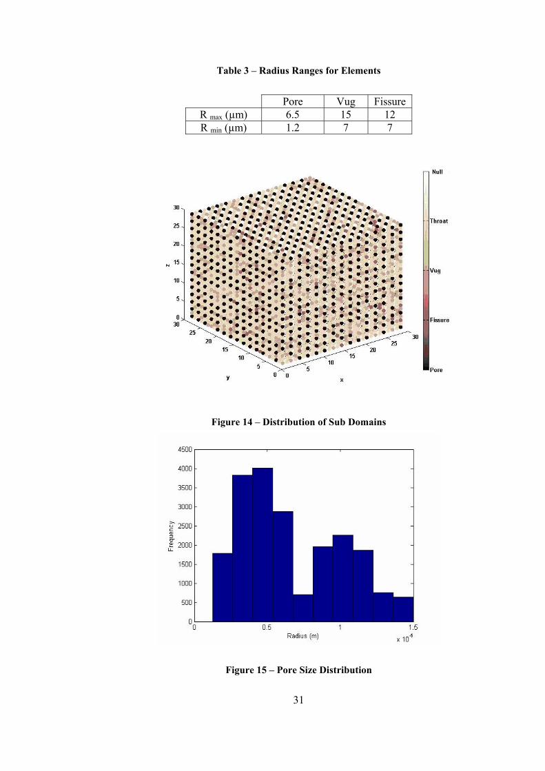
31
Table 3 – Radius Ranges for Elements
Pore Vug Fissure
R max (µm) 6.5 15 12 R min (µm) 1.2 7 7
Figure 14 – Distribution of Sub Domains
Figure 15 – Pore Size Distribution
32
The type of cross sections is defined by corner half angle values (α) of elements
and area of an element is calculated by considering α (Equation 14), by not
directly using geometric equations (Hui and Blunt, 2000).
cotαRnA 2ct ⋅⋅= (14)
Contact angle ranges are selected by bearing in mind that porous media is mixed
wet and water is always present in corners. In addition, receeding angle range is
assigned such that advancing angle is always greater than receeding angle.
Presence of water in corners is guaranteed by the relationship between receeding
and corner angles (Equation 15).
παθReceeding ≤+ (15)
5.2. Simulation of Flow Mechanisms
5.2.1. Primary Drainage
5.2.1.1. Threshold Pressure Calculation
For simulating two – phase flow in this pore network model, first primary
drainage is considered. It is assumed that the system is filled by water prior to oil
migration. In primary drainage, receeding angle values are used as contact angle
and non-wetting phase enters an element with radius R at threshold pressure of Pc
(Oren and et al., 1997);
( ) F
RcosθπG21σPc
+= (16)
where;
πG21θ4GD/cos11F
2
+++
= (17)
33
4Gθcos-3sinθsinθ
pi/3θ1πD
2
+⎟⎟⎠
⎞⎜⎜⎝
⎛−= (18)
2
2
11
)sin(2α)sin(2α2
2)sin(2αG
−
⎟⎟⎠
⎞⎜⎜⎝
⎛+⋅= (19)
Since the elements are represented by regular geometries, αi (where i=1, 2,..,nc)
values are equal. During primary drainage, receeding angle is used as contact
angle (θ).
5.2.1.2. Primary Drainage Algorithm
Flow of non-wetting phase starts from y=1 to y=29 and all of the elements (pore,
throat, fissure or vug) connected to inlet are considered to be prospective elements
to be invaded. Initially, threshold pressures of all elements are calculated by using
Equation 16 and corresponding pressure values of the inlet elements are listed. An
element with minimum threshold pressure is filled by non-wetting phase and
current capillary pressure of the system is set to this value. Then, its neighbor
elements are controlled to find out whether they can be invaded or not. If a
particular capillary pressure exceeds the corresponding threshold pressure of the
neighbor element, it is filled and its capillary pressure is set equal to current
capillary pressure. If threshold pressure of the neighbor element is greater than the
current capillary pressure, the element is added into the pressure list.
Subsequently, the minimum pressure in the list is set equal to the capillary
pressure of the system and its corresponding element is filled. The same
procedure is applied until all possible elements are invaded by non-wetting phase.
At each filling step, saturation and conductance of both phases are calculated.
At the end of primary drainage, water is present in corners and oil is in center of
the invaded elements. Oil/water contact can be either pinned or not and it is
determined by the receeding angle and the corner half angle.
34
5.2.2. Waterflooding (Imbibition)
Waterflooding starts after primary drainage and two-phase flow properties of the
model are obtained for imbibition. All possible flow mechanisms in imbibition,
snap-off, piston-like advance and pore body filling, are considered. During
imbibition, advancing angle values are used as contact angle. As mentioned
before, advancing contact angle values are normally distributed between 30 and
160 degrees range yielding a mixed – wet system. All possible fluid
configurations are examined, thus saturation and conductance calculations are
conducted by bearing in mind the presence of oil layers, if exists any.
5.2.2.1. Snap – Off
During waterflooding, occurrence of snap – off is controlled first. As mentioned
before, if Roof’s criterion (Equation 1) is satisfied, the element is assumed to be
filled by snap – off process (Jia, 2005). The preference between spontaneous and
forced snap – off is determined by relationship between corner half angle and
contact angle. Threshold pressure of an element can be obtained for snap – off
mechanism by using Equations 2 and 3.
In spontaneous snap – off, if θh > θa, the element is assumed to be completely
filled by wetting phase present in corners. Otherwise, phase configuration does
not change (same as at the end of primary drainage). In forced snap – off, oil /
water contact is pinned if θh < θa and Ac is determined by using θh otherwise, π- θa
is used as θ. In case of θ= (π/ 2) – α, the element is completely filled by wetting
phase and conductance is calculated accordingly.
5.2.2.2. Piston – Like Advance
In piston – like advance, imbibition can be either spontaneous or forced and the
preference depends on θAdvancing and θMax (Oren and Bakke, 1997). In spontaneous
imbibition, the element is completely filled by the invading wetting phase. As
35
hinging angle reaches advancing angle, the element will be completely filled by
wetting phase. Contrary to spontaneous case, in forced imbibition oil layers can be
preserved when suitable conditions exist. In case of forced imbibition, capillary
pressure is negative and wetting phase has two components (in corner and in
center). Thus, wetting and non – wetting phase areas are calculated by accounting
for the presence of oil layers.
Threshold pressure in spontaneous imbibition is calculated by using the
aforementioned iterative method (Equations 5-8). During spontaneous imbibition,
an element is completely filled by wetting phase and conductance is calculated
straightforwardly. In forced imbibition, threshold pressure is obtained by Equation
10 and presence of oil layers is controlled by Equation 9. In case of oil layers,
wetting phase has two components; corners and center. Total conductance of
wetting phase is obtained by summation of these components. If oil layers are not
preserved, the element will be completely filled by wetting – phase and
conductance is obtained correspondingly.
5.2.2.3. Pore Body Filling
In pore body filling mechanism, number of previously invaded elements is
important. If only one invaded neighbor element (I1) is present, imbibition will be
same as piston – like advance. Threshold pressure and conductance will be
calculated by using the same procedure for piston – like advance.
Pore body filling mechanism can occur either spontaneously (θ≤θmax) or forced
(θ≤θmax). In spontaneous imbibition, threshold pressure is calculated by using
Equations 11 and 12 and number of terms depends on the number of previously
invaded neighbor elements (Oren and Bakke, 1997). As for forced imbibition,
threshold pressure is obtained as I1 mechanism. Phase conductances are
determined correspondingly for either spontaneous or forced imbibition.
36
5.2.2.4. Waterflooding Algorithm
Waterflooding starts after primary drainage and flow occurs from y=1 to y=29.
Initially, threshold pressure values, for all waterflooding mechanisms, are
calculated for invaded elements in primary drainage. The inlet elements are
assumed to be filled by piston-like advance mechanism. For the interior and outlet
elements, there is competition between the imbibition mechanisms. First, element
is checked for snap-off using Roof’s criterion. If snap-off is not favored, threshold
pressures for piston like advance and pore body filling mechanisms are compared.
Mechanism yielding greater threshold pressure is favored for the corresponding
element (Jia, 2005). Then, threshold pressures of inlet elements are listed and
element with maximum threshold value is invaded by wetting-phase and its
threshold pressure is set equal to current capillary pressure of the system. The
neighbors of the invaded element are checked to be filled by wetting phase or not.
If it can be invaded, saturation and conductance of the element is calculated. If the
neighbor can not be invaded, its threshold pressure is added into the list and
procedure continues until the all possible elements are invaded by wetting-phase.
Similar to primary drainage, at each filling step, saturation and conductance of
both wetting and non-wetting phases are calculated.
5.2.3. Calculation of Flow Properties
5.2.3.1. Phase Area Calculation
For saturation and conductance calculations, wetting and non-wetting phases’
areas are determined. Phase areas in the corners and in the center (Figure 16) are
calculated by the following formulae (Piri and Blunt, 2005).
( ) ⎪⎪⎭
⎪⎪⎬
⎫
⎪⎪⎩
⎪⎪⎨
⎧
≠+⎟⎠⎞
⎜⎝⎛ −++−
=+⎟⎠⎞
⎜⎝⎛ +
=
2πθα if ,
2πsincoscotcosrn
2πθα if , cossin
sinαα)cos(θR
A2
c
2
c
αθθθαθ
αα (20)
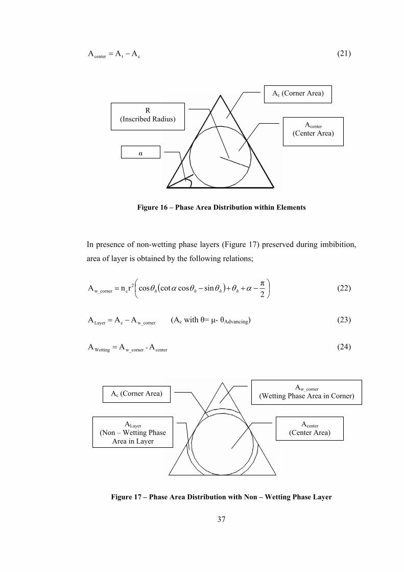
37
ctcenter AAA −= (21)
Figure 16 – Phase Area Distribution within Elements In presence of non-wetting phase layers (Figure 17) preserved during imbibition,
area of layer is obtained by the following relations;
( ) ⎟⎠⎞
⎜⎝⎛ −++−=
2πsincoscotcosrn A 2
cw_corner αθθθαθ hhhh (22)
w_cornercLayer AAA −= (Ac with θ= μ- θAdvancing) (23)
center w_cornerWetting AAA += (24)
Figure 17 – Phase Area Distribution with Non – Wetting Phase Layer
ALayer (Non – Wetting Phase
Area in Layer
Aw_corner (Wetting Phase Area in Corner) Ac (Corner Area)
Acenter (Center Area)
α
R (Inscribed Radius)
Ac (Corner Area)
Acenter (Center Area)
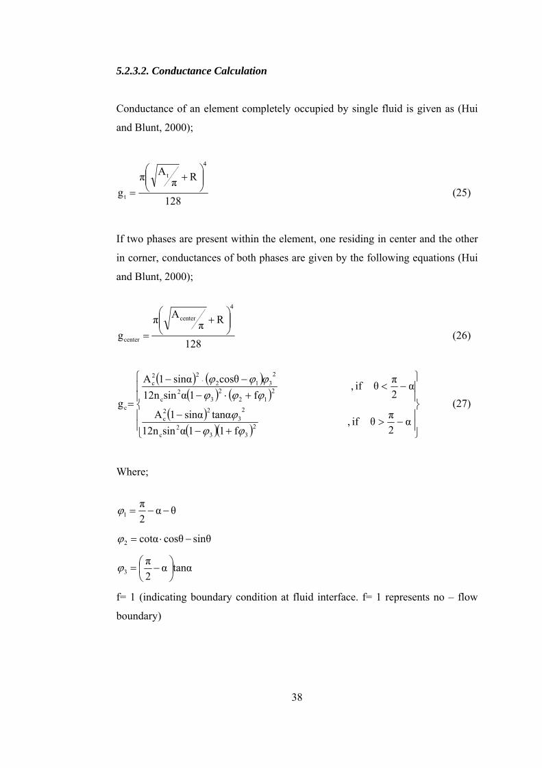
38
5.2.3.2. Conductance Calculation
Conductance of an element completely occupied by single fluid is given as (Hui
and Blunt, 2000);
128
RπAπ
g
4
t
t
⎟⎟⎠
⎞⎜⎜⎝
⎛+
= (25)
If two phases are present within the element, one residing in center and the other
in corner, conductances of both phases are given by the following equations (Hui
and Blunt, 2000);
128
RπAπ
g
4
center
center
⎟⎟⎠
⎞⎜⎜⎝
⎛+
= (26)
( ) ( )
( ) ( )( )
( )( ) ⎪⎪
⎭
⎪⎪
⎬
⎫
⎪⎪
⎩
⎪⎪
⎨
⎧
−>+−
−
−<+⋅−−−
=
⋅
α2πθ if ,
f11αsin12ntanαsinα1A
α2πθ if ,
f1αsin12ncosθsinα1A
g
233
2c
23
22c
212
23
2c
2312
22c
c
ϕϕϕ
ϕϕϕϕϕϕ
(27)
Where;
θα2π
1 −−=ϕ
sinθcosθcotα2 −⋅=ϕ
tanαα2π
3 ⎟⎠⎞
⎜⎝⎛ −=ϕ
f= 1 (indicating boundary condition at fluid interface. f= 1 represents no – flow
boundary)
39
At the end of the imbibition process, if non – wetting phase is preserved as layer
within elements, corresponding wetting and non – wetting phase conductances are
obtained by following equations (Hui and Blunt, 2000);
( )
( )2
c
w_corner32313
2cc
23
23Layer
Layer
AA
)f(1f11αsinA12n
tanαsinα1Ag
⎟⎟⎠
⎞⎜⎜⎝
⎛−−+⋅−
−=
ϕϕϕ
ϕ (28)
w_cornercenterwetting ggg += (29)
Where gw_corner is calculated by using Ac=Aw_corner.
5.2.3.3. Saturation Calculation
Saturation of each phase within an element is obtained by the ratio of phase area
to the total area of the model. At each filling step, phase saturations are obtained
by the summation of saturations of corresponding phase at each element.
T
pp A
AS = (30)
∑==
Num
1i T
i pT A
AS (31)
5.2.3.4. Relative Permeability Calculation
In pore network modeling studies, Poiseuille’s law is applied and phase flow rates
are obtained. Then, relative permeability is obtained by dividing the phase flow
rate to total flow rate of the system.(Oren and Bakke, 1997; Patzek, 2000; Piri and
Blunt, 2005). In this study, relative permeability is defined as the ratio of phase
conductance to total conductance of the system in order to minimize time
consumption. Since the model is initially filled by water, total conductance of the
40
system is defined with respect to water conductance. Total conductance and
relative permeability of a particular element are defined as;
∑+
==
⎟⎟⎠
⎞⎜⎜⎝
⎛
Num
1i
4
iit
T 128
RπAπ
g (32)
T
Num
1ii p
rp g
gk
∑= = (33)
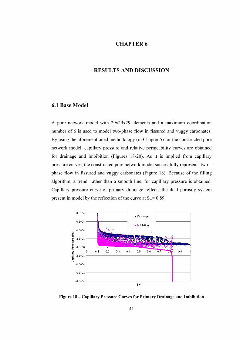
41
CHAPTER 6
RESULTS AND DISCUSSION
6.1 Base Model
A pore network model with 29x29x29 elements and a maximum coordination
number of 6 is used to model two-phase flow in fissured and vuggy carbonates.
By using the aforementioned methodology (in Chapter 5) for the constructed pore
network model, capillary pressure and relative permeability curves are obtained
for drainage and imbibition (Figures 18-20). As it is implied from capillary
pressure curves, the constructed pore network model successfully represents two –
phase flow in fissured and vuggy carbonates (Figure 18). Because of the filling
algorithm, a trend, rather than a smooth line, for capillary pressure is obtained.
Capillary pressure curve of primary drainage reflects the dual porosity system
present in model by the reflection of the curve at Sw= 0.89.
Figure 18 – Capillary Pressure Curves for Primary Drainage and Imbibition
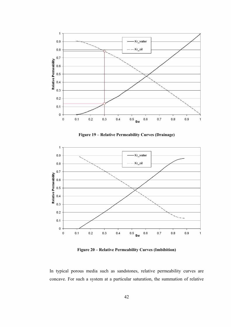
42
Figure 19 – Relative Permeability Curves (Drainage)
Figure 20 – Relative Permeability Curves (Imbibition) In typical porous media such as sandstones, relative permeability curves are
concave. For such a system at a particular saturation, the summation of relative
43
permeabilities is less than one, indicating phase interference. On the other than,
for fractured media X – type relative permeability curves are reported (Romm,
1966). That is to say, the summation of relative permeability values at a particular
saturation is equal to 1 (no phase interference). However, recent studies (Akın,
2001) indicate that concave relative permeability curves are possible for fractured
media. In the present study, relative permeability curves are obtained for primary
drainage and imbibition (Figures 19 and 20). It is observed that the curves are
neither concave nor linear. This is validated by the summation of relative
permeability values at a particular saturation. For example, for primary drainage,
at Sw= 0.3, water relative permeability is 0.14 where as oil relative permeability is
near 0.78 (summation is 0.92), indicating phase interference.Valvatne (2004)
reported capillary pressure and relative permeability curves for a mixed – wet
intergranular carbonate sample. The sample has pores and throat with 0.1 μm
radius mainly. He obtained capillary pressure curve for primary drainage with
receeding angles in 25-65 range, fixed advancing angle of 140° and interfacial
tension of 0.48 N/m for mercury and air. Capillary pressure curve obtained for the
same wettability conditions is compared with the one in Valvatne’s study (Figure
21) with adjusted pore base model (Table 4). Also, capillary pressure curve
obtained in this study is smoothed as representing the general trend for
comparison. Effects of secondary porosity features are not recognizable since
smaller radius ranges for the elements are assigned (Table 4) resulting in a
relatively homogeneous porous media. On the other hand, in relative permeability
curves, secondary porosity effects are amplified (Figure 22). Valvatne used
intergranular carbonate sample which was relatively homogeneous and reported
concave relative permeability curves. Base model (for fissured and vuggy
carbonate rock) is modified for simulating primary drainage with the same
wettability conditions (Table 4). It is observed that due to the secondary porosity
features the model resulted in linear relative permeability curves (Figure 22).
Also, cross over points are at close water saturations with different relative
permeabilities. This is due to the flow algorithm used in this study and pore
morphology. In other words, greater element sizes resulted higher saturation and
conductance.
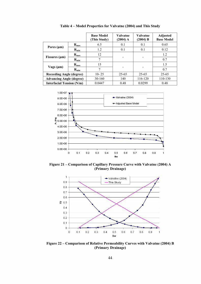
44
Table 4 – Model Properties for Valvatne (2004) and This Study
Base Model (This Study)
Valvatne (2004) A
Valvatne (2004) B
Adjusted Base Model
Rmax 6.5 0.1 0.1 0.65 Pores (μm)
Rmin 1.2 0.1 0.1 0.12 Rmax 12 1.2
Fissures (μm) Rmin 7
- - 0.7
Rmax 15 1.5 Vugs (μm)
Rmin 7 - -
0.7 Receeding Angle (degree) 10- 25 25-65 25-65 25-65 Advancing Angle (degree) 30-160 140 116-120 110-130 Interfacial Tension (N/m) 0.0447 0.48 0.0299 0.48
Figure 21 – Comparison of Capillary Pressure Curve with Valvatne (2004) A (Primary Drainage)
Figure 22 – Comparison of Relative Permeability Curves with Valvatne (2004) B
(Primary Drainage)
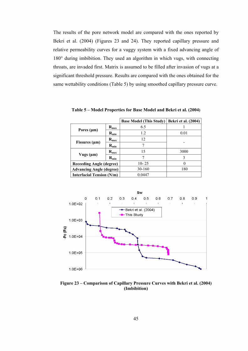
45
The results of the pore network model are compared with the ones reported by
Bekri et al. (2004) (Figures 23 and 24). They reported capillary pressure and
relative permeability curves for a vuggy system with a fixed advancing angle of
180° during imbibition. They used an algorithm in which vugs, with connecting
throats, are invaded first. Matrix is assumed to be filled after invasion of vugs at a
significant threshold pressure. Results are compared with the ones obtained for the
same wettability conditions (Table 5) by using smoothed capillary pressure curve.
Table 5 – Model Properties for Base Model and Bekri et al. (2004)
Base Model (This Study) Bekri et al. (2004) Rmax 6.5 1
Pores (μm) Rmin 1.2 0.01 Rmax 12
Fissures (μm) Rmin 7
-
Rmax 15 3000 Vugs (μm)
Rmin 7 3 Receeding Angle (degree) 10- 25 0 Advancing Angle (degree) 30-160 180 Interfacial Tension (N/m) 0.0447
Figure 23 – Comparison of Capillary Pressure Curves with Bekri et al. (2004) (Imbibition)
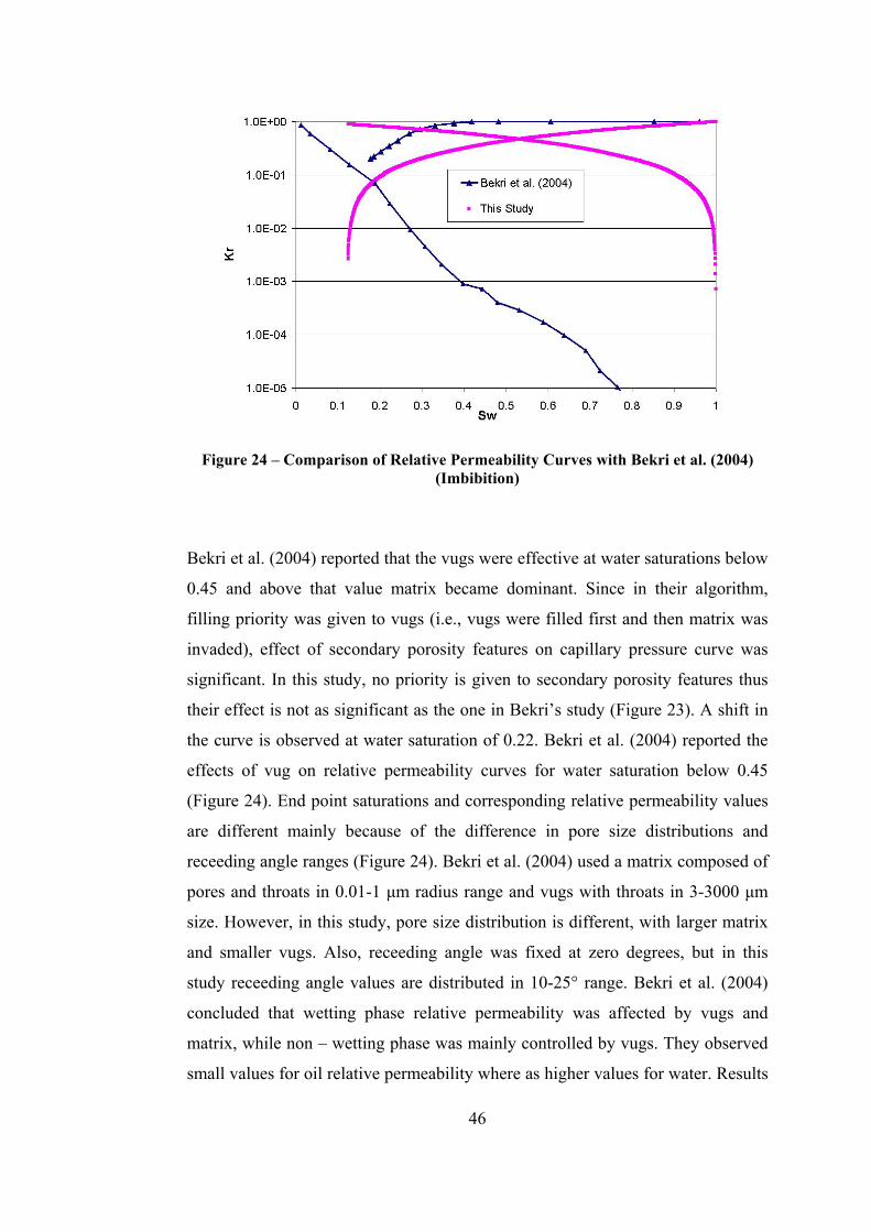
46
Figure 24 – Comparison of Relative Permeability Curves with Bekri et al. (2004) (Imbibition)
Bekri et al. (2004) reported that the vugs were effective at water saturations below
0.45 and above that value matrix became dominant. Since in their algorithm,
filling priority was given to vugs (i.e., vugs were filled first and then matrix was
invaded), effect of secondary porosity features on capillary pressure curve was
significant. In this study, no priority is given to secondary porosity features thus
their effect is not as significant as the one in Bekri’s study (Figure 23). A shift in
the curve is observed at water saturation of 0.22. Bekri et al. (2004) reported the
effects of vug on relative permeability curves for water saturation below 0.45
(Figure 24). End point saturations and corresponding relative permeability values
are different mainly because of the difference in pore size distributions and
receeding angle ranges (Figure 24). Bekri et al. (2004) used a matrix composed of
pores and throats in 0.01-1 μm radius range and vugs with throats in 3-3000 μm
size. However, in this study, pore size distribution is different, with larger matrix
and smaller vugs. Also, receeding angle was fixed at zero degrees, but in this
study receeding angle values are distributed in 10-25° range. Bekri et al. (2004)
concluded that wetting phase relative permeability was affected by vugs and
matrix, while non – wetting phase was mainly controlled by vugs. They observed
small values for oil relative permeability where as higher values for water. Results
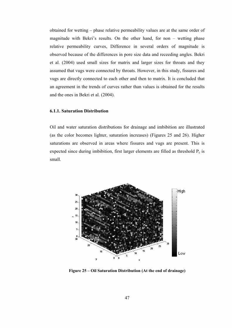
47
obtained for wetting – phase relative permeability values are at the same order of
magnitude with Bekri’s results. On the other hand, for non – wetting phase
relative permeability curves, Difference in several orders of magnitude is
observed because of the differences in pore size data and receeding angles. Bekri
et al. (2004) used small sizes for matrix and larger sizes for throats and they
assumed that vugs were connected by throats. However, in this study, fissures and
vugs are directly connected to each other and then to matrix. It is concluded that
an agreement in the trends of curves rather than values is obtained for the results
and the ones in Bekri et al. (2004).
6.1.1. Saturation Distribution
Oil and water saturation distributions for drainage and imbibition are illustrated
(as the color becomes lighter, saturation increases) (Figures 25 and 26). Higher
saturations are observed in areas where fissures and vugs are present. This is
expected since during imbibition, first larger elements are filled as threshold Pc is
small.
Figure 25 – Oil Saturation Distribution (At the end of drainage)
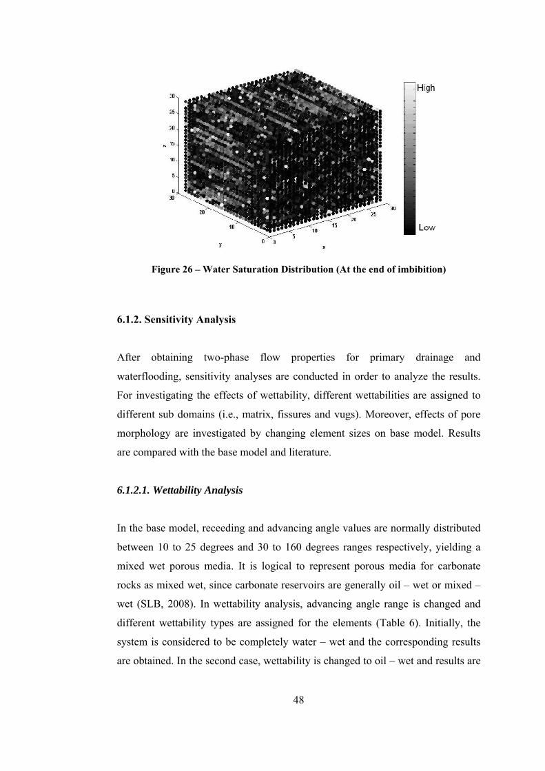
48
Figure 26 – Water Saturation Distribution (At the end of imbibition)
6.1.2. Sensitivity Analysis
After obtaining two-phase flow properties for primary drainage and
waterflooding, sensitivity analyses are conducted in order to analyze the results.
For investigating the effects of wettability, different wettabilities are assigned to
different sub domains (i.e., matrix, fissures and vugs). Moreover, effects of pore
morphology are investigated by changing element sizes on base model. Results
are compared with the base model and literature.
6.1.2.1. Wettability Analysis
In the base model, receeding and advancing angle values are normally distributed
between 10 to 25 degrees and 30 to 160 degrees ranges respectively, yielding a
mixed wet porous media. It is logical to represent porous media for carbonate
rocks as mixed wet, since carbonate reservoirs are generally oil – wet or mixed –
wet (SLB, 2008). In wettability analysis, advancing angle range is changed and
different wettability types are assigned for the elements (Table 6). Initially, the
system is considered to be completely water – wet and the corresponding results
are obtained. In the second case, wettability is changed to oil – wet and results are
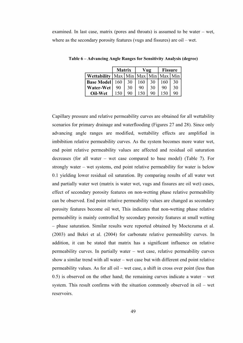
49
examined. In last case, matrix (pores and throats) is assumed to be water – wet,
where as the secondary porosity features (vugs and fissures) are oil – wet.
Table 6 – Advancing Angle Ranges for Sensitivity Analysis (degree)
Matrix Vug Fissure Wettability Max Min Max Min Max Min Base Model 160 30 160 30 160 30 Water-Wet 90 30 90 30 90 30
Oil-Wet 150 90 150 90 150 90 Capillary pressure and relative permeability curves are obtained for all wettability
scenarios for primary drainage and waterflooding (Figures 27 and 28). Since only
advancing angle ranges are modified, wettability effects are amplified in
imbibition relative permeability curves. As the system becomes more water wet,
end point relative permeability values are affected and residual oil saturation
decreases (for all water – wet case compared to base model) (Table 7). For
strongly water – wet systems, end point relative permeability for water is below
0.1 yielding lower residual oil saturation. By comparing results of all water wet
and partially water wet (matrix is water wet, vugs and fissures are oil wet) cases,
effect of secondary porosity features on non-wetting phase relative permeability
can be observed. End point relative permeability values are changed as secondary
porosity features become oil wet, This indicates that non-wetting phase relative
permeability is mainly controlled by secondary porosity features at small wetting
– phase saturation. Similar results were reported obtained by Moctezuma et al.
(2003) and Bekri et al. (2004) for carbonate relative permeability curves. In
addition, it can be stated that matrix has a significant influence on relative
permeability curves. In partially water – wet case, relative permeability curves
show a similar trend with all water – wet case but with different end point relative
permeability values. As for all oil – wet case, a shift in cross over point (less than
0.5) is observed on the other hand; the remaining curves indicate a water – wet
system. This result confirms with the situation commonly observed in oil – wet
reservoirs.
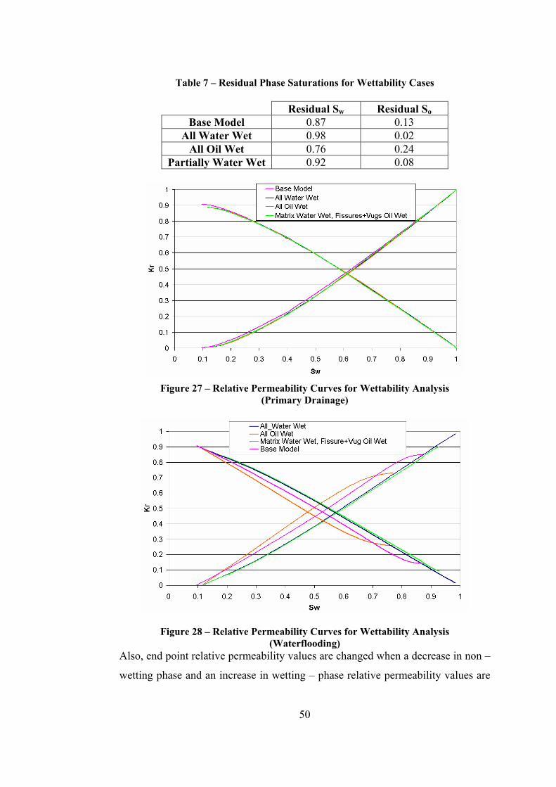
50
Table 7 – Residual Phase Saturations for Wettability Cases
Residual Sw Residual So
Base Model 0.87 0.13 All Water Wet 0.98 0.02
All Oil Wet 0.76 0.24 Partially Water Wet 0.92 0.08
Figure 27 – Relative Permeability Curves for Wettability Analysis
(Primary Drainage)
Figure 28 – Relative Permeability Curves for Wettability Analysis (Waterflooding)
Also, end point relative permeability values are changed when a decrease in non –
wetting phase and an increase in wetting – phase relative permeability values are
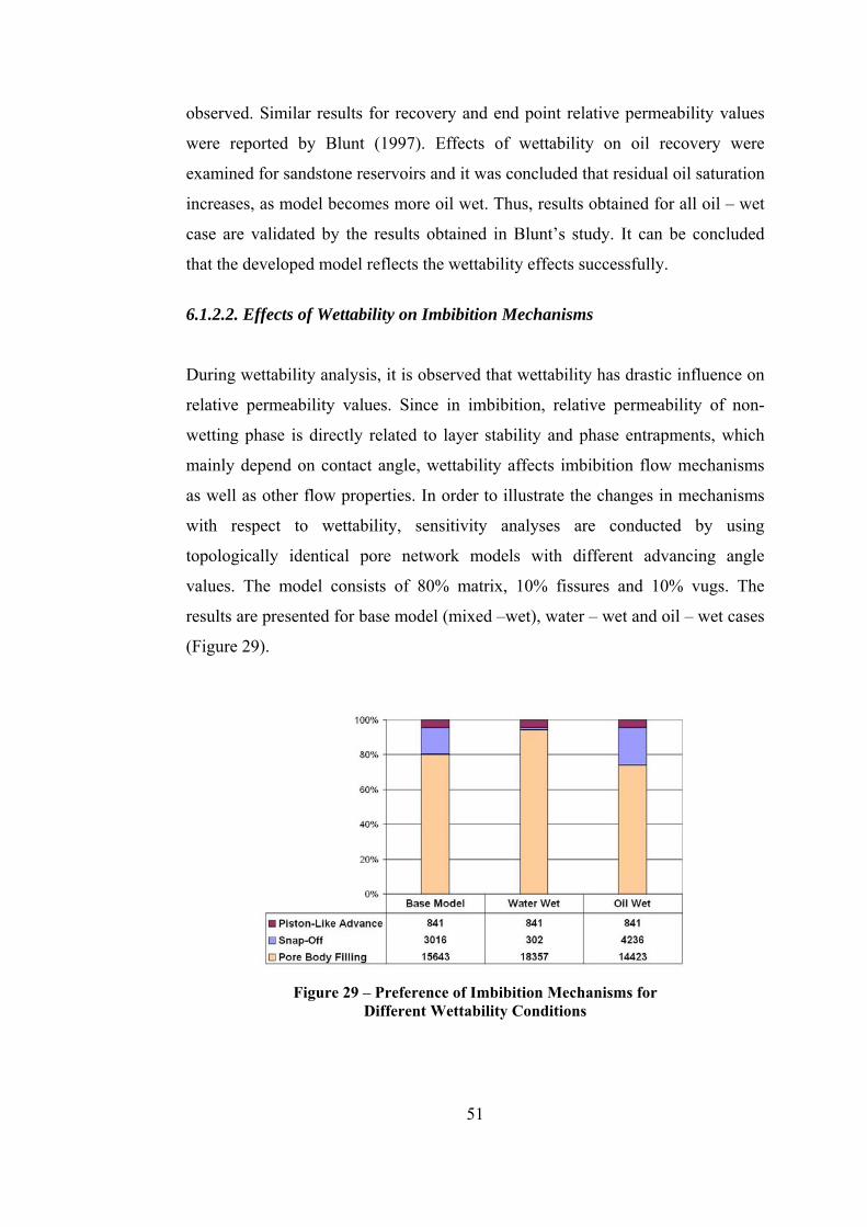
51
observed. Similar results for recovery and end point relative permeability values
were reported by Blunt (1997). Effects of wettability on oil recovery were
examined for sandstone reservoirs and it was concluded that residual oil saturation
increases, as model becomes more oil wet. Thus, results obtained for all oil – wet
case are validated by the results obtained in Blunt’s study. It can be concluded
that the developed model reflects the wettability effects successfully.
6.1.2.2. Effects of Wettability on Imbibition Mechanisms
During wettability analysis, it is observed that wettability has drastic influence on
relative permeability values. Since in imbibition, relative permeability of non-
wetting phase is directly related to layer stability and phase entrapments, which
mainly depend on contact angle, wettability affects imbibition flow mechanisms
as well as other flow properties. In order to illustrate the changes in mechanisms
with respect to wettability, sensitivity analyses are conducted by using
topologically identical pore network models with different advancing angle
values. The model consists of 80% matrix, 10% fissures and 10% vugs. The
results are presented for base model (mixed –wet), water – wet and oil – wet cases
(Figure 29).
Figure 29 – Preference of Imbibition Mechanisms for
Different Wettability Conditions
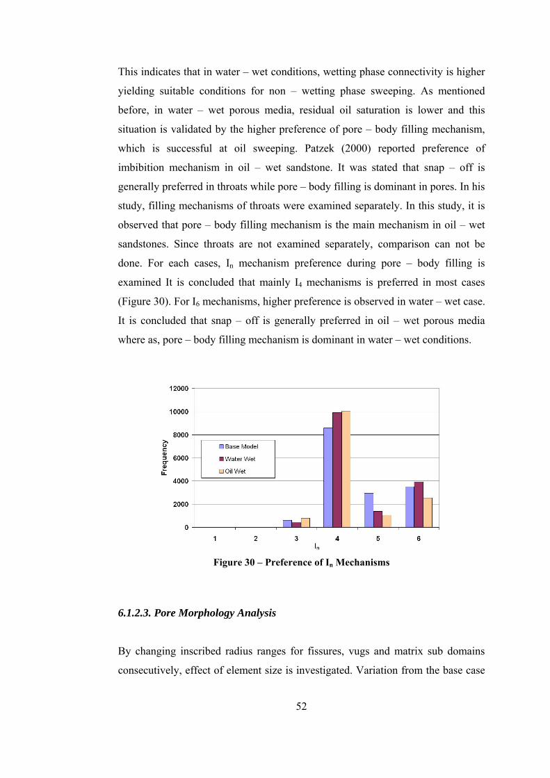
52
This indicates that in water – wet conditions, wetting phase connectivity is higher
yielding suitable conditions for non – wetting phase sweeping. As mentioned
before, in water – wet porous media, residual oil saturation is lower and this
situation is validated by the higher preference of pore – body filling mechanism,
which is successful at oil sweeping. Patzek (2000) reported preference of
imbibition mechanism in oil – wet sandstone. It was stated that snap – off is
generally preferred in throats while pore – body filling is dominant in pores. In his
study, filling mechanisms of throats were examined separately. In this study, it is
observed that pore – body filling mechanism is the main mechanism in oil – wet
sandstones. Since throats are not examined separately, comparison can not be
done. For each cases, In mechanism preference during pore – body filling is
examined It is concluded that mainly I4 mechanisms is preferred in most cases
(Figure 30). For I6 mechanisms, higher preference is observed in water – wet case.
It is concluded that snap – off is generally preferred in oil – wet porous media
where as, pore – body filling mechanism is dominant in water – wet conditions.
Figure 30 – Preference of In Mechanisms
6.1.2.3. Pore Morphology Analysis
By changing inscribed radius ranges for fissures, vugs and matrix sub domains
consecutively, effect of element size is investigated. Variation from the base case
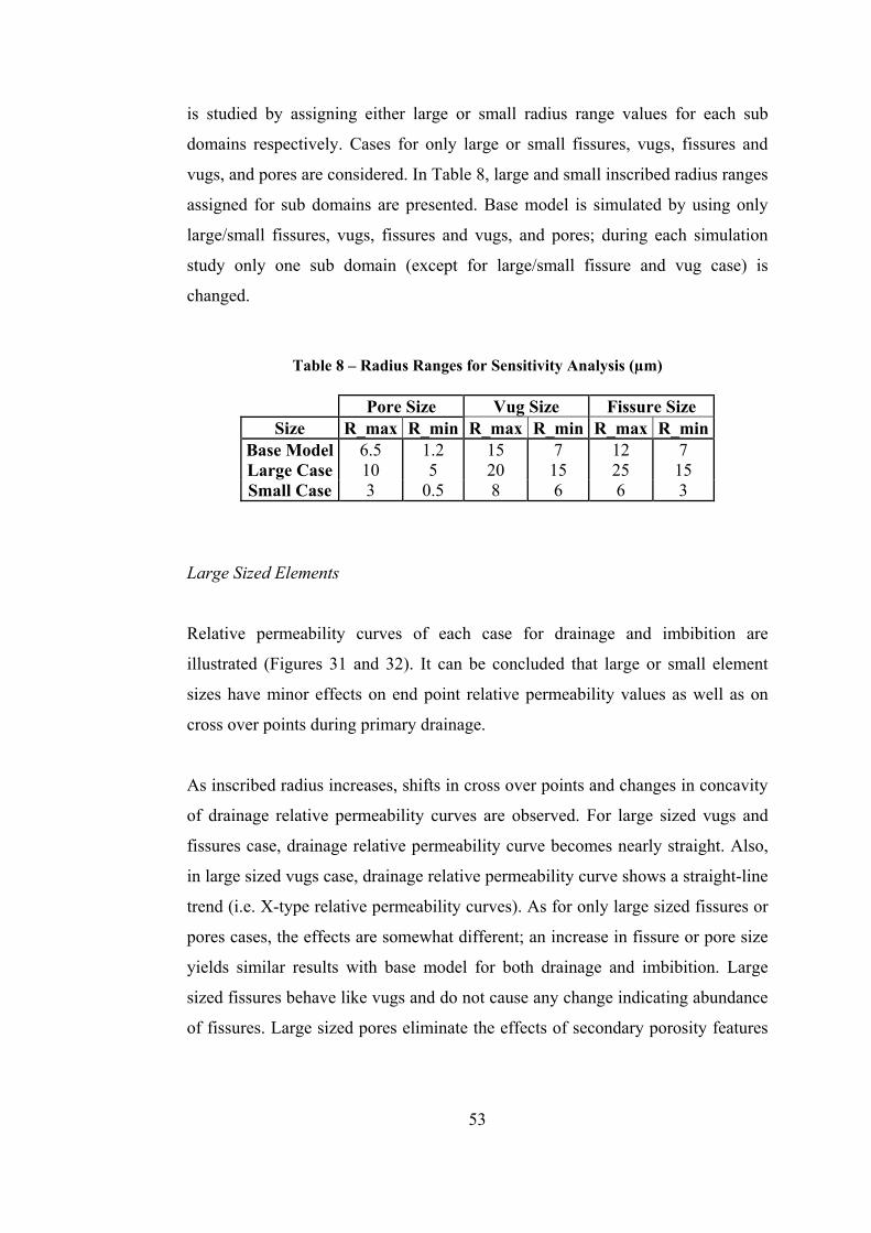
53
is studied by assigning either large or small radius range values for each sub
domains respectively. Cases for only large or small fissures, vugs, fissures and
vugs, and pores are considered. In Table 8, large and small inscribed radius ranges
assigned for sub domains are presented. Base model is simulated by using only
large/small fissures, vugs, fissures and vugs, and pores; during each simulation
study only one sub domain (except for large/small fissure and vug case) is
changed.
Table 8 – Radius Ranges for Sensitivity Analysis (µm)
Pore Size Vug Size Fissure Size Size R_max R_min R_max R_min R_max R_min
Base Model 6.5 1.2 15 7 12 7 Large Case 10 5 20 15 25 15 Small Case 3 0.5 8 6 6 3
Large Sized Elements
Relative permeability curves of each case for drainage and imbibition are
illustrated (Figures 31 and 32). It can be concluded that large or small element
sizes have minor effects on end point relative permeability values as well as on
cross over points during primary drainage.
As inscribed radius increases, shifts in cross over points and changes in concavity
of drainage relative permeability curves are observed. For large sized vugs and
fissures case, drainage relative permeability curve becomes nearly straight. Also,
in large sized vugs case, drainage relative permeability curve shows a straight-line
trend (i.e. X-type relative permeability curves). As for only large sized fissures or
pores cases, the effects are somewhat different; an increase in fissure or pore size
yields similar results with base model for both drainage and imbibition. Large
sized fissures behave like vugs and do not cause any change indicating abundance
of fissures. Large sized pores eliminate the effects of secondary porosity features
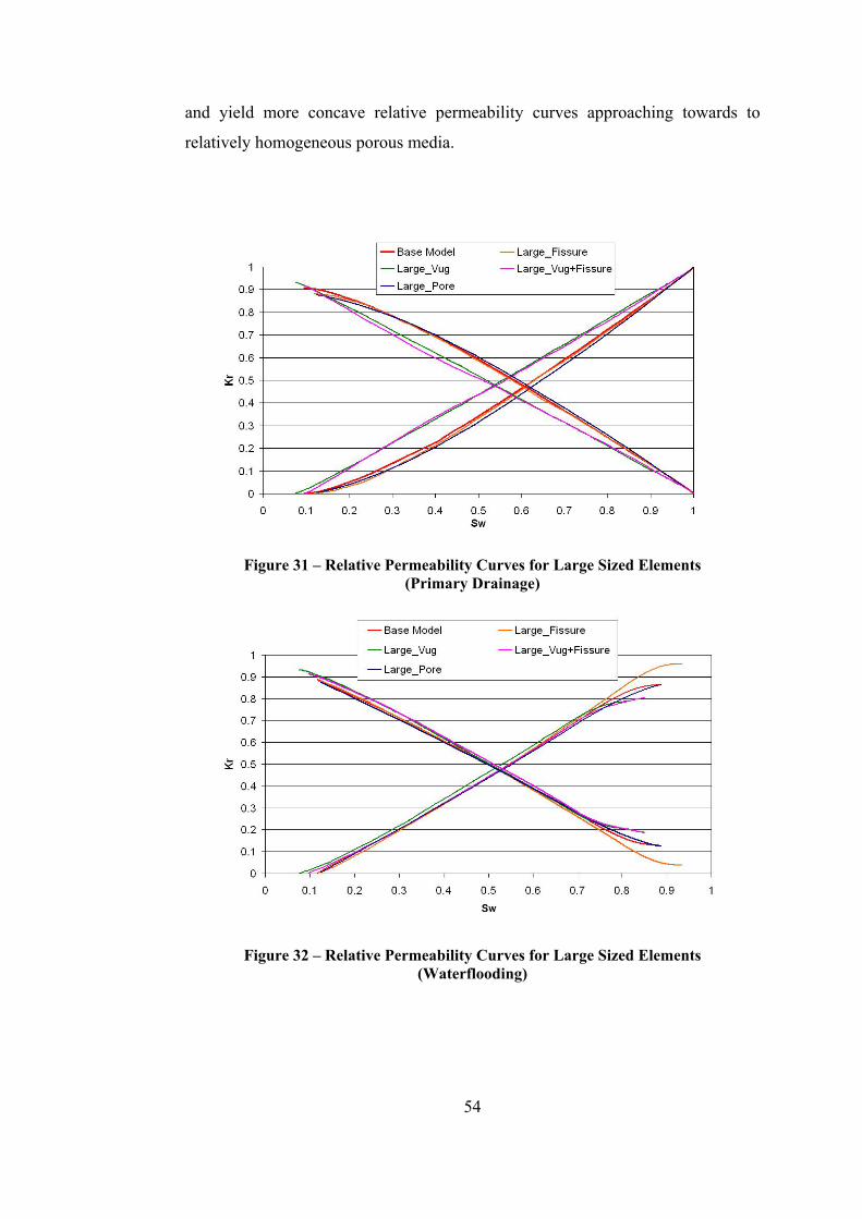
54
and yield more concave relative permeability curves approaching towards to
relatively homogeneous porous media.
Figure 31 – Relative Permeability Curves for Large Sized Elements (Primary Drainage)
Figure 32 – Relative Permeability Curves for Large Sized Elements (Waterflooding)

55
It can be concluded that for large sized elements, especially vugs and fissures,
porous media behaves like fractured or microfractured porous medium. Similar
results were reported previously (Romm, 1966; Babadagli and Ershaghi, 1993;
Wilson-Lopez and Rodriguez, 2004). Larger vugs and fissures also effect
imbibition by yielding higher end point water relative permeability values; larger
vugs and fissures, and vug cases, result a system which has less water – wet
behavior than the base model. As mentioned before, as the system becomes more
oil – wet (a shift in cross over saturation towards left), residual oil saturation
increases and thus end point oil relative permeability decreases significantly. It
can be stated that size of secondary porosity features, in other words secondary
porosity value, obviously affect non – wetting phase recovery and wettability
behavior of a system.
Small Sized Elements
Small values for radius ranges are assigned and pore network model with small
sized elements is constructed. Two-phase relative permeability curves for primary
drainage and imbibition processes are illustrated (Figure 33 and 34). During
primary drainage, effects of small sized vugs and pores are more obvious with
respect to small sized fissures or fissures and vugs cases. As vugs get smaller,
they act like pores and reduce the effect of secondary porosity features thus,
relative permeability curves become more concave with respect to base model
curve approaching towards to a single porosity system. Contrary to small sized
vugs case, small sized pores significantly increase the effects of secondary
porosity features during primary drainage. Thus, curvature of relative
permeability curves decreases and they become straighter reflecting a fractured
system.
As for small sized fissure and small sized vug and fissure cases, the effects are not
obvious in primary drainage and imbibition. Similar results with the base model
are obtained but minor increases in end point water relative permeability are
observed in primary drainage curves.
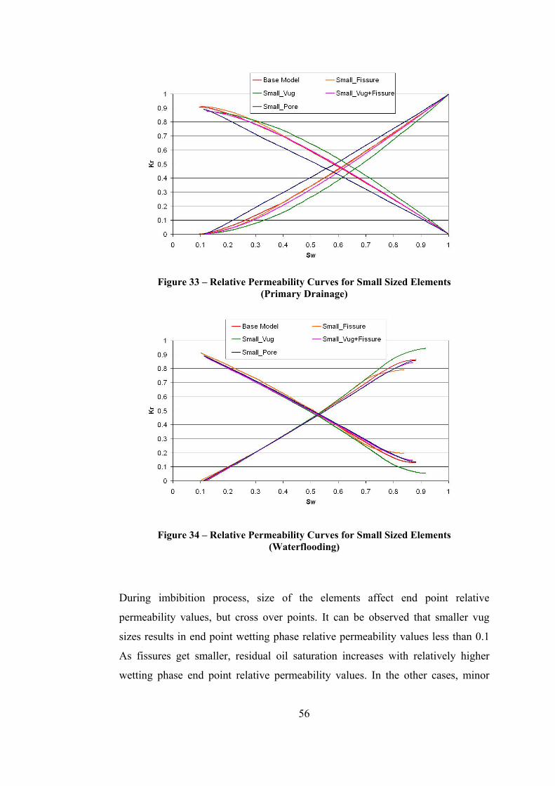
56
Figure 33 – Relative Permeability Curves for Small Sized Elements (Primary Drainage)
Figure 34 – Relative Permeability Curves for Small Sized Elements (Waterflooding)
During imbibition process, size of the elements affect end point relative
permeability values, but cross over points. It can be observed that smaller vug
sizes results in end point wetting phase relative permeability values less than 0.1
As fissures get smaller, residual oil saturation increases with relatively higher
wetting phase end point relative permeability values. In the other cases, minor
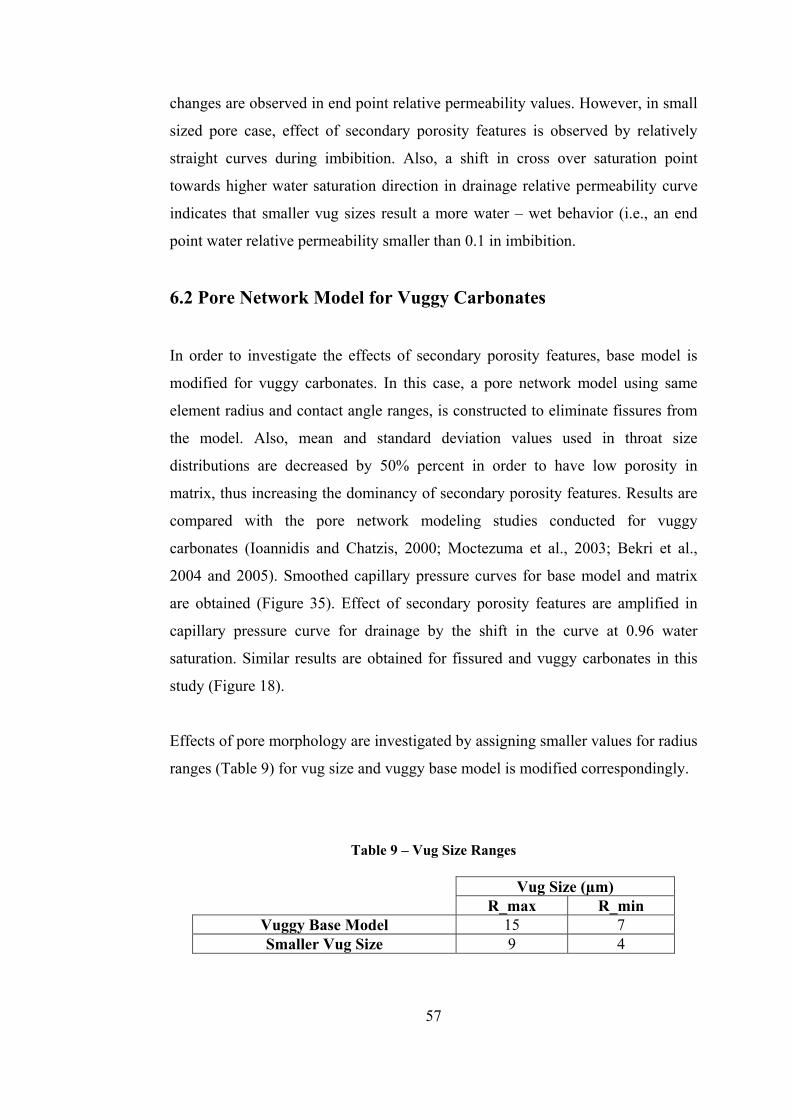
57
changes are observed in end point relative permeability values. However, in small
sized pore case, effect of secondary porosity features is observed by relatively
straight curves during imbibition. Also, a shift in cross over saturation point
towards higher water saturation direction in drainage relative permeability curve
indicates that smaller vug sizes result a more water – wet behavior (i.e., an end
point water relative permeability smaller than 0.1 in imbibition.
6.2 Pore Network Model for Vuggy Carbonates
In order to investigate the effects of secondary porosity features, base model is
modified for vuggy carbonates. In this case, a pore network model using same
element radius and contact angle ranges, is constructed to eliminate fissures from
the model. Also, mean and standard deviation values used in throat size
distributions are decreased by 50% percent in order to have low porosity in
matrix, thus increasing the dominancy of secondary porosity features. Results are
compared with the pore network modeling studies conducted for vuggy
carbonates (Ioannidis and Chatzis, 2000; Moctezuma et al., 2003; Bekri et al.,
2004 and 2005). Smoothed capillary pressure curves for base model and matrix
are obtained (Figure 35). Effect of secondary porosity features are amplified in
capillary pressure curve for drainage by the shift in the curve at 0.96 water
saturation. Similar results are obtained for fissured and vuggy carbonates in this
study (Figure 18).
Effects of pore morphology are investigated by assigning smaller values for radius
ranges (Table 9) for vug size and vuggy base model is modified correspondingly.
Table 9 – Vug Size Ranges
Vug Size (µm) R_max R_min
Vuggy Base Model 15 7 Smaller Vug Size 9 4
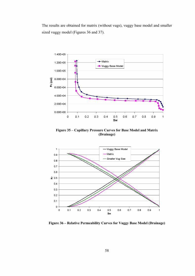
58
The results are obtained for matrix (without vugs), vuggy base model and smaller
sized vuggy model (Figures 36 and 37).
Figure 35 – Capillary Pressure Curves for Base Model and Matrix (Drainage)
Figure 36 – Relative Permeability Curves for Vuggy Base Model (Drainage)
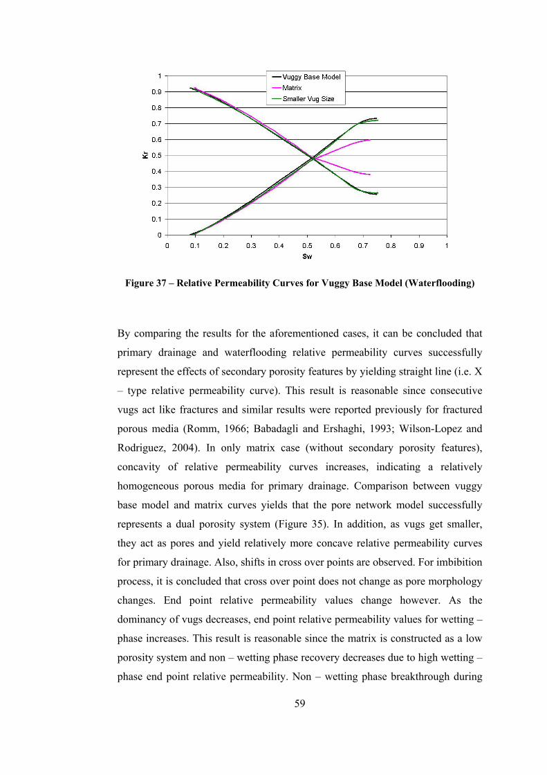
59
Figure 37 – Relative Permeability Curves for Vuggy Base Model (Waterflooding) By comparing the results for the aforementioned cases, it can be concluded that
primary drainage and waterflooding relative permeability curves successfully
represent the effects of secondary porosity features by yielding straight line (i.e. X
– type relative permeability curve). This result is reasonable since consecutive
vugs act like fractures and similar results were reported previously for fractured
porous media (Romm, 1966; Babadagli and Ershaghi, 1993; Wilson-Lopez and
Rodriguez, 2004). In only matrix case (without secondary porosity features),
concavity of relative permeability curves increases, indicating a relatively
homogeneous porous media for primary drainage. Comparison between vuggy
base model and matrix curves yields that the pore network model successfully
represents a dual porosity system (Figure 35). In addition, as vugs get smaller,
they act as pores and yield relatively more concave relative permeability curves
for primary drainage. Also, shifts in cross over points are observed. For imbibition
process, it is concluded that cross over point does not change as pore morphology
changes. End point relative permeability values change however. As the
dominancy of vugs decreases, end point relative permeability values for wetting –
phase increases. This result is reasonable since the matrix is constructed as a low
porosity system and non – wetting phase recovery decreases due to high wetting –
phase end point relative permeability. Non – wetting phase breakthrough during
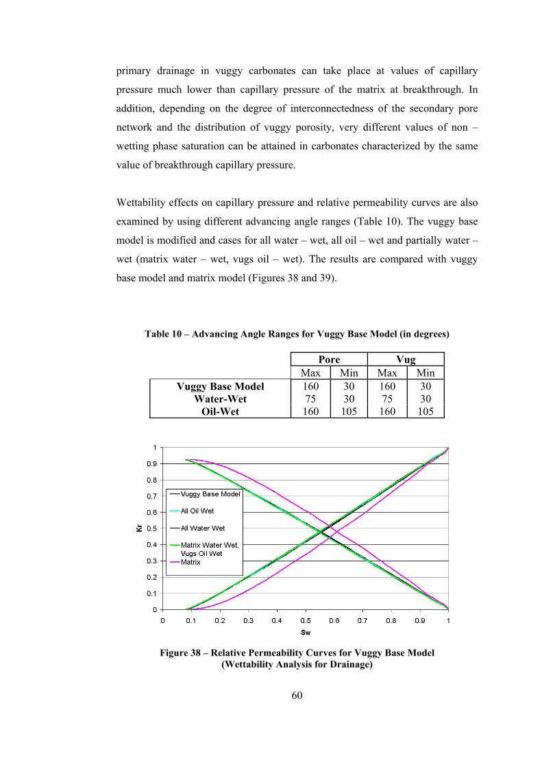
60
primary drainage in vuggy carbonates can take place at values of capillary
pressure much lower than capillary pressure of the matrix at breakthrough. In
addition, depending on the degree of interconnectedness of the secondary pore
network and the distribution of vuggy porosity, very different values of non –
wetting phase saturation can be attained in carbonates characterized by the same
value of breakthrough capillary pressure.
Wettability effects on capillary pressure and relative permeability curves are also
examined by using different advancing angle ranges (Table 10). The vuggy base
model is modified and cases for all water – wet, all oil – wet and partially water –
wet (matrix water – wet, vugs oil – wet). The results are compared with vuggy
base model and matrix model (Figures 38 and 39).
Table 10 – Advancing Angle Ranges for Vuggy Base Model (in degrees)
Pore Vug Max Min Max Min
Vuggy Base Model 160 30 160 30 Water-Wet 75 30 75 30
Oil-Wet 160 105 160 105
Figure 38 – Relative Permeability Curves for Vuggy Base Model
(Wettability Analysis for Drainage)
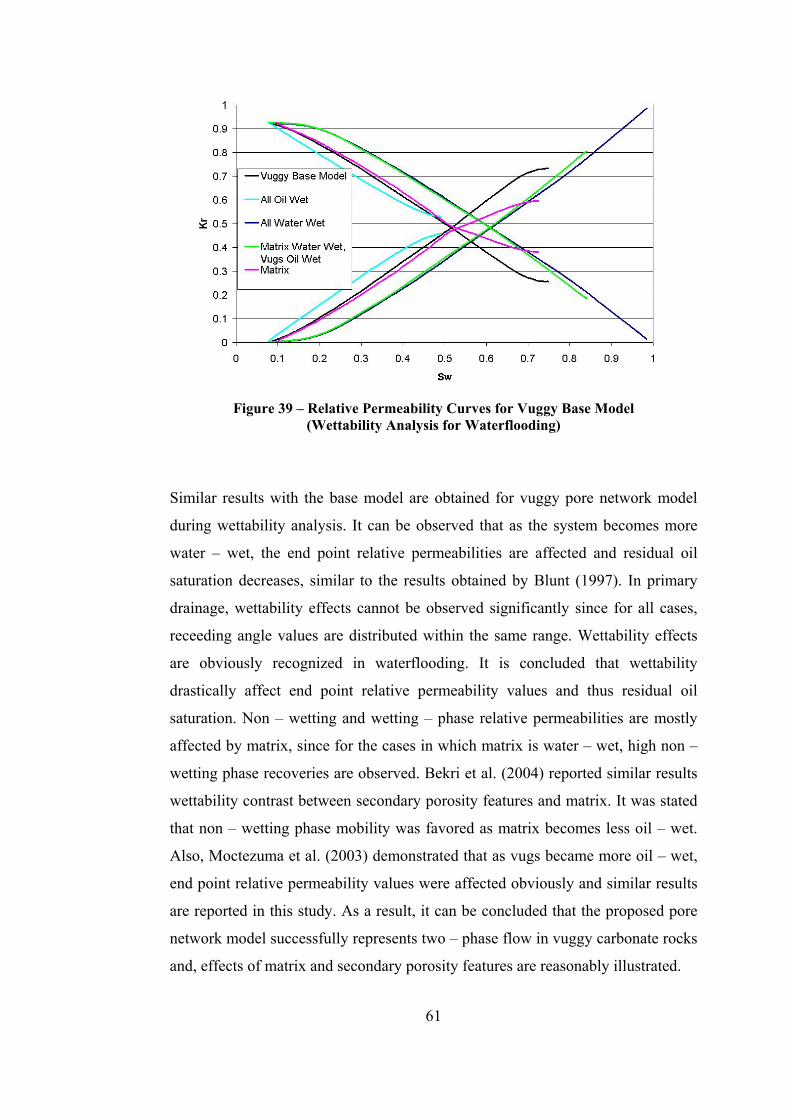
61
Figure 39 – Relative Permeability Curves for Vuggy Base Model
(Wettability Analysis for Waterflooding) Similar results with the base model are obtained for vuggy pore network model
during wettability analysis. It can be observed that as the system becomes more
water – wet, the end point relative permeabilities are affected and residual oil
saturation decreases, similar to the results obtained by Blunt (1997). In primary
drainage, wettability effects cannot be observed significantly since for all cases,
receeding angle values are distributed within the same range. Wettability effects
are obviously recognized in waterflooding. It is concluded that wettability
drastically affect end point relative permeability values and thus residual oil
saturation. Non – wetting and wetting – phase relative permeabilities are mostly
affected by matrix, since for the cases in which matrix is water – wet, high non –
wetting phase recoveries are observed. Bekri et al. (2004) reported similar results
wettability contrast between secondary porosity features and matrix. It was stated
that non – wetting phase mobility was favored as matrix becomes less oil – wet.
Also, Moctezuma et al. (2003) demonstrated that as vugs became more oil – wet,
end point relative permeability values were affected obviously and similar results
are reported in this study. As a result, it can be concluded that the proposed pore
network model successfully represents two – phase flow in vuggy carbonate rocks
and, effects of matrix and secondary porosity features are reasonably illustrated.
62
CHAPTER 7
CONCLUSIONS
Two-phase flow in fissured and vuggy carbonates was studied by developing a
new pore network model that consists of several sub-networks including matrix,
vug and fissures. The matrix was constructed as spatially correlated since pore
and throat radii were statistically related, where as the secondary porosity features
were assigned randomly yielding a spatially uncorrelated pore network model.
Primary drainage and imbibition processes were simulated and corresponding
flow properties were determined. In order to investigate the effects of wettability
on flow properties and mechanisms in heterogeneous carbonate rocks, sensitivity
analyses were conducted for different wettability types. In addition, effects of
pore morphology were examined and results were compared with the base model
and literature. The following conclusions are drawn from the results obtained in
this study:
• Heterogeneous porous media can be successfully represented by
sub networks composed of matrix and secondary porosity features
similar to the one constructed in this study,
• Wettability significantly influences on capillary pressure and
relative permeability curves and thus residual oil saturation. End
point relative permeability values are directly affected by
wettability type.

63
• As the system becomes more water wet, residual oil saturation
decreases and end point water relative permeassbility increases.
This indicates that, higher recovery is favored for strongly water –
wet systems, as it is reported in literature previously.
• In heterogeneous carbonates, matrix wettability directly affects end
point relative permeability values. As matrix becomes oil – wet
recovery decreases.
• It is observed that wettability type also influences on flow
mechanisms, snap – off, piston –like advance and pore body filling,
during imbibition. The preference between the mechanisms
depends on contact angle and as system becomes water – wet, pore
body filling mechanism is favored. In oil – wet systems, snap – off
is mainly preferred.
• Pore morphology directly affects flow properties especially during
primary drainage. As sizes of secondary porosity features increase,
the system behaves like fractured media yielding linear relative
permeability curves. As vugs and fissures get smaller, effect of
secondary porosity features decreases and concavity of relative
permeability curves increases.
• As vugs and fissures get larger, cross over point shifts to lower
wetting phase saturation for primary drainage. This indicates that
wettability behavior of a system is altered by changes in element
size.
• For imbibition, change in pore morphology results drastic changes
in end point relative permeability values. It is concluded that as
size of secondary porosity features get smaller, end point relative
permeability value of wetting phase increases.
64
CHAPTER 8
RECOMMENDATIONS
Pore network modeling is an effective tool in identification of flow mechanisms
and determination of flow properties. By using the developed model in this study,
it is shown that two – phase flow can be simulated in fissured and vuggy
carbonates at pore scale. Also, effects of wettability on capillary pressure and
relative permeability curves are examined. In this study, relative permeability
values are determined by a new approach, rather than using Poiseuille’s law.
Improved studies can be conducted in order to compare the results obtained by
using the aforementioned methodology and the ones obtained from Poiseuille’s
law and typical flow equations.
Further research studies can be conducted by using the aforementioned model and
methodology, to determine three phase flow properties. Mechanisms like WAG or
polymer injection can be simulated and corresponding flow properties, which are
challenging to be determined experimentally, can be obtained. Moreover, by using
pore space extraction tools, topologically equivalent pore network model can be
used to simulate two or three phase flow in heterogeneous carbonates.
65
REFERENCES
Akin,S.,“Estimation of Fracture Relative Permeabilities From Unsteady State
Corefloods”, Journal of Petroleum Science and Engineering, 30, 2001, 1-14.
Al-Futaisi, A., Patzek, T. W., “Secondary Imbibition in NAPL- Invaded
Mixed Wet Sediments”, Journal of Contaminant Hydrology, 74, 2004, 61-81.
Al-Kharusi, A. S. Z., “Pore Scale Characterization of Carbonate Rocks”, PhD
Thesis, Imperial College, 2007.
Archie, G.E., “Classification of Carbonate Reservoir Rocks and Petrophysical
Considerations”, AAPG Bulletin, 36-6, 1952, 278-298.
Babadagli, T., Ershaghi, I., “Improved Modeling of Oil/Water Flow in
Naturally Fractured Reservoirs Using Effective Fracure Relative
Permeabilities”, SPE 26076, Proceedings of the 1993 SPE Western Regional
Meeting, Anchorage, Alaska, USA, 1993.
Bakke, S., Oren, P. E., “3-D Pore Scale Modeling of Sandstones and Flow
Simulations in the Pore Network”, SPE 35479, SPE Journal, Vol. 2, June
1997, 136-149.
Balhoff, M., “Modeling the Flow of Non-Newtonian Fluids in Packed Beds at
the Pore Scale”, PhD Thesis, Louisiana State University, 2005.
66
Bekri, S., Laroche, C., Vizika, O., “Pore Network Models to Calculate
Transport and Electrical Properties of Single or Dual- Porosity Rocks”, SCA
2005-35, Proceedings of 2005 International Symposium of the Society of Core
Analysts, Toronto, Canada, 2005.
Bekri, S., Nardi, C., Vizika, O., “Effect of Wettability on the Petrophysical
Parameters of Vuggy Carbonates: Network Modeling Investigation”, SCA
2004-25, Proceedings of 2004 International Symposium of the Society of Core
Analysts, Abu Dhabi, UAE, 2004.
Blunt, M., J, King, M., J, “Simulation and Theory of Two Phase Flow in
Porous Media”, Physical Review A, 46-12, December 1992, 7680-7702.
Blunt, M.J., “Flow in Porous Media – Pore Network Models and Multiphase
Flow”, Current Opinion in Colloid & Interface Science, 6, 2001, 197-207.
Blunt, M.J., “Pore Level Modeling of the Effects of Wettability”, SPE Journal,
2, December 1997, 494-510.
Choquette, P.W, Pray, L.C., “Geologic Nomenclature and Classification of
Porosity in Sedimentary Carbonates”, AAPG Bulletin, 54, 1970, 207-250.
Dias, M. M., Payatakes, A. C., “Network Models for Two Phase Flow in
Porous Media: 1. Immiscible Microdisplacement of Nonwetting Fluids”,
Journal of Fluid Mechanics, 164, 1986, 305-336.
Dodds, J.A., Lloyd, P.J., “A Model for the Void Structure in Multi-
Component Sphere Packs Applied to Capillary Pressure Curves”, Powder
Technology, 5, 1971, 69- 76.
Dullien, F.A.L., “Porous Media: Fluid Transport and Pore Structure”, 1992,
San Diego, California: Academic Press Inc.
67
Dullien, F.A.L., Chatzis, I., El-Sayed, M.S., “Modeling Transport Phenomena
in Porous Media by Networks Consisting of Non-Uniform Tubes”, SPE 6191,
Proceedings of the 1976 Annual Fall Technical Conference and Exhibition of
SPE of AIME, New Orleans, 1976.
Dunham, R.J., “Classification of Carbonate Rocks According to Depositional
Texture”, Proceeding of AAPG Classification of Carbonate Rocks: A
Symposium, 1962, 108-121.
Erzeybek, S., Akin, S., “Pore Network Modeling of Multiphase Flow in
Fissured and Vuggy Carbonates”, SPE 113384, Proceedings of the 2008
SPE/DOE Improved Oil Recovery Symposium, Tulsa, OK, 2008.
Fatt, I., “The Network Model of Porous Media I. Capillary Pressure
Characteristics”, Trans. AIME, 207, 1956, 144.
Fatt, I., “The Network Model of Porous Media II. Dynamic Properties of a
Single Size Tube Network”, Trans. AIME, 207, 1956, 160.
Fatt, I., “The Network Model of Porous Media III. Dynamic Properties of
Networks with Tube Radius Distribution”, Trans. AIME, 207, 1956, 164.
Fenwick, D.H., Blunt, M.J., “Network Modeling of Three-Phase Flow in
Porous Media”, SPE Journal, March 1998, 86-97.
Hatiboğlu, C. H., “Automated Porosity Measurement Using Image Analysis
Techniques”, M.Sc. Thesis, Middle East Technical University, 2002.
Heiba, A.A., Davis, H.T., Scriven, L.E., “Effect of Wettability on Two-Phase
Relative Permeabilities and Capillary Pressures”, SPE 12172, Proceedings of
the 1983 SPE Annual Technical Conference and Exhibition, San Francisco,
CA, 1983.
68
Honarpour, M., Mahmood, S.M., SPE 18565, Relative Permeability
Measurements: An Overview, SPE Technology Today Series, 1986.
Hughes, R.G., Blunt, M.J., “Network Modeling of Multiphase Flow in
Fractures”, Advances in Water Resources, 24, 2001, 409-421.
Hughes, R.G., Blunt, M.J., “Pore Scale Modeling of Rate Effects in
Imbibition”, Transport in Porous Media, 40, 2000, 295-322.
Hui, M.H., Blunt, M.J., “Pore Scale Modeling of Three-Phase Flow and the
Effects of Wettability”, SPE 59309, Proceedings of the 2000 SPE/DOE
Improved Oil Recovery Symposium, Tulsa, OK, 2000.
Ioannidis, M.A., Chatzis, I., “A Dual-Network Model of Pore Structure for
Vuggy Carbonates”, SCA 2000-09, Proceedings of 2000 International
Symposium of the Society of Core Analysts, Abu Dhabi, UAE, 2000.
Jardine, D., Andrews, D. P., Wischart, J. W., Young, J. W., “Distribution and
Continuity of Carbonate Reservoirs”, SPE 6139, Journal of Petroleum
Technology, July 1977, 873-885.
Jia, C., Shing, K., Yortsos, Y. C., “Visualization and Simulation of Non-
Aqueous Phase Liquids Solubilization in Pore Networks”, Journal of
Contaminant Hydrology, 35, 1999, 363-387.
Jia, L., “Reservoir Definition through Integration of Multiscale Petrophysical
Data”, Ph.D. Thesis, Stanford University, 2005.
Jin, G., Patzek, T. W., “Physics-Based Reconstruction of Sedimentary Rocks”,
SPE 83587, Proceeding of SPE Western Regional/ AAPG Pacific Section
Joint Meeting, Long Beach, California, USA, 19-24 May, 2003.
69
Kamath, J., Xu, B., Lee, S.H., Yortsos, Y.C., “Use of Pore Network Models to
Interpret Laboratory Experiments on Vugular Rocks”, Journal of Petroleum
Science and Technology, 20, 1998, 109-115.
Karaman, T., “Development of a Pore Network Model and a Neural Network
Model To Be Coupled To Simulate Porous Medium”, M.Sc. Thesis, Middle
East Technical University, 2002.
Knackstedt, M. A., Sheppard, A. P., Sahimi, M., “Pore Network Modeling of
Two Phase Flow in Porous Rock: The Effect of Correlated Heterogeneity”,
Advances in Water Resources, 24, 2001, 257 – 277.
Koplick, J., Lasseter, T.J., “Two Phase Flow in Random Network Models of
Porous Media”, SPEJ, February 1985, 89-100.
Larson, R.G., Scriven, L.E., Davis, H.T., “Percolation Theory of Two Phase
Flow in Porous Media”, Chemical Engineering Science, 36, 1981, 57-73.
Lenormand, R., Toubol, E., Zarcone, C., “Numerical Models and Experiments
on Another in a Network of Capillary Ducts”, Journal of Fluid Mechanics,
186, 1988, 165-187.
Lopez, X., Valvatne, P. H., Blunt, M. J., “Predictive Network Modeling of
Single Phase Non-Newtonian Flow in Porous Media”, Journal of Colloid and
Interface Science, 264, 2003, 256-265.
Lu, C., Yortsos, Y. C., “A Pore Network Model of In-Situ Combustion in
Porous Media”, SPE 69705, Proceeding of SPE International Thermal
Operations and Heavy Oil Symposium, Margarita, Venezuela, 12-14 March,
2001.
70
Lucia, F.J., “Petrophysical Parameters Estimated from Visual Descriptions of
Carbonate Rocks: A Field Classification of Carbonate Pore Space”, Journal of
Petroleum Technology, March 1983, 629- 637.
Lucia, F. J., Carbonate reservoir characterization, Berlin, Germany, Springer, 1999.
Mani, V., Mohanty, K. K., “Effect of Pore – Space Spatial Correlations on
Two – Phase Flow in Porous Media”, Journal of Petroleum Science and
Engineering, 23, 1999, 173 – 188.
Mazullo, S. J., “Overview of Porosity Evolution in Carbonate Rocks”, Kansas
Geological Society Bulletin, 79, 1, 2004.
Moctezuma, A., Bekri, S., Laroche, C., Vizika, O., “A Dual Network Model
for Relative Permeability of Bimodal Rocks: Application in a Vuggy
Carbonate”, SCA2003-12, Proceedings of 2003 International Symposium of
the Society of Core Analysts, Pau, France, 2003.
Mogensen, K., Stenby, E.H., “A Dynamic Two-Phase Pore-Scale Model of
Imbibition”, Transport in Porous Media, 32, 1998, 299-327.
Moore, C.H., “Carbonate Reservoirs Porosity Evolution and Diagenesis in a
Sequence Stratigraphic Framework”, 2001, Amsterdam, The Netherlands,
Elsevier Scientific Publ. Co.
Murray, R.C., “Origin of Porosity in Carbonate Rocks”, Journal of
Sedimentary Petrology, 30, 1, 1960, 59-84.
Nguyen, V.H., Sheppard, A.P., Knackstedt, M.A., Pinczewski, W.V., “The
Effects of Displacement Rate and Wettability on Imbibition Relative
Permeabilities”, SCA2005-39, Proceedings of 2005 International Symposium
of the Society of Core Analysts, Toronto, Canada, 2005.
71
Nilsen, L. S., Oren, P.E. and Bakke, S., “Prediction of Relative Permeability
and Capillary Pressure from a Pore Model”, SPE 35531, Proceedings of the
European 3-D Reservoir Modeling Conference, Stavanger, Norway, 1996.
Okabe, H., “Pore Scale Modeling of Carbonates”, Ph.D. Thesis, University of
London, Diploma, Imperial College, 2004.
Oren, P.E., Bakke, S., Arntzen, O.J., “Extending Predictive Capabilities to
Network Models”, SPE 38880, Proceedings of the 1997 SPE Annual
Technical Conference and Exhibition, San Antonio, Texas, 1997.
Patzek, T. W., Silin, D.B., “Shape Factor and Hydraulic Conductance in
Noncircular Capillaries I. One-Phase Creeping Flow”, Journal of Colloid and
Interface Science, 236, 2001, 295-304.
Patzek, T.W., “Verification of a Complete Pore Network Simulator of
Drainage and Imbibition”, SPE 59312, Proceedings 2000 of the SPE/DOE
Improved Oil Recovery Symposium, Tulsa, OK, 2000.
Peacock, D.C.P., Mann, A “Evaluation of the Controls on Fracturing in
Reservoir Rocks”, Journal of Petroleum Geology, 28-4, 2005, 385-396.
Piri, M., “Pore-Scale Modeling of Three-Phase Flow”, Ph.D. Thesis, Imperial
College, 2003.
Piri, M., Blunt, M.J., “Three- Dimensional Mixed Wet Random Pore Scale
Network Modeling of Two and Three Phase Flow in Porous Media I. Model
Description”, Physical Review E., 71, 2005, 26301/1-26301-30.
72
Radke, C.J., Kovscek, A.R., Wong, H., “A Pore-Level Scenario for the
Development of Mixed Wettability in Oil Reservoirs”, SPE 24880,
Proceedings of the 1992 SPE Annual Technical Conference and Exhibition,
Washington, DC, 1992.
Romm, E.S., “Fluid Flow in Fractured Rocks”, Nedra Publishing House,
Moscow, 1966.
SLB, Schlumberger, Carbonate Reservoirs, (Last accessed in April, 2008)
http://www.slb.com/media/services/solutions/reservoir/carbonate_reservoirs.p
Sochi, T., “Pore-Scale Modeling of Non-Newtonian Flow in Porous Media”,
PhD Thesis, Imperial College, 2007.
Tomeczek, J., Mlonka, J., “The Parameters of a Random Pore Network with
Spherical Vesicles for Coal Structure Modeling”, Fuel, Vol. 77, 15, 1998,
1841-1844.
Uzun, I., “Use Of Pore Scale Simulators to Understand the Effects of
Wettability on Miscible Carbon Dioxide Flooding and Injectivity”, M.Sc.
Thesis, Middle East Technical University, 2005.
Valvatne, P.H., “Predicting Pore-Scale Modeling of Multiphase Flow”, Ph.D.
Thesis, Imperial College, 2004.
Valvatne, P.H., Blunt, M.J., “Predictive Pore-Scale Network Modeling”, SPE
84550, Proceedings of the 2003 SPE Annual Technical Conference and
Exhibition, Denver, Colorado, 2003.
Wilkinson, D., Willemsen, J.F., “Invasion Percolation: A New Form of
Percolation Theory”, Journal of Physics A: Math. Gen., 1983, 16, 3365-3376.

73
Wilson-Lopez, R.V., Rodriguez, F., “A Network Model for Two-Phase Flow
in Microfractures Porous Media”, SPE 92056, Proceedings of 2004 SPE
International Petroleum Conference, Puebla, Mexico, 2004.
74
APPENDIX A
MATLAB CODE FOR PORE NETWORK CONSTRUCTION
%Matrix Construction Function (17.10.2007) function [Model]=model_const(R_max,R_min,x,a,c,Approach,min,max,mu,sig,n) clear all fid1=fopen('pore_size.dat','r'); fid2=fopen('pore_properties.dat','r'); fid3=fopen('model_prop.dat','r'); fid4=fopen('contact_angles.dat','r'); fid5=fopen('pore_throat_size.dat','r+'); fid6=fopen('fissure_size.dat','r'); fid7=fopen('vug_size.dat', 'r'); pore_prop; pore_throat; Pore_Model_Cons; model; g_w; %===== Pore Properties Function=========== %Inscribed radius calculation,total area calculation and pore size distribution function [At,R_ins,alpha,nc] =pore_prop(R_max,R_min,x,a,c,Approach,n) global At R_ins alpha n nc n_p theta_0 theta_1 theta_ow %Lengths are in meter n=fscanf(fid3, '%g %g',[1,1]); %model size n_p=n^3; %number of pores Radius=fscanf(fid1,'%g', [2,n_p]); %Radius values are gathered. %Constants, From Blunt (2000) delta=0.3; gamma=1.8; x=0+(1-0)*rand(n_p,1); %Inscribed radius calculation R_max=0.000006535; R_min=0.000001206; R_ins=(R_max-R_min).*(-delta*log(x.*(1-exp(-1/delta))+exp(-1/delta))).^(1/gamma)+R_min; %Inscribed Radius %Distribution maximum=max2(R_ins)/2; minimum=min2(R_ins)/2; m=mean(R_ins)/2; s=std(R_ins)/2; range_vals=[maximum;minimum;m;s]; fprintf(fid5,'%g\n', range_vals);
75
fclose(fid5) hist(R_ins) prop=fscanf(fid2,'%g',[1,3]); a=prop(1); if a==1; dist1= normpdf(R_ins,m,s); end if a==2; dist2= lognpdf(R_ins,m,s); end %Cross section type and total area calculation Approach=prop(2); c=prop(3); %Cross section type (Square:1, Equilateral Triangle:2, Circular:3) %Alpha is half-angle of each corner of a polygon if Approach==1; %Blunt's Total Area Approach disp('Blunts Total Area Approach is used') if c==1; alpha=pi()/4; %For square,in radians nc=4; %# of corners At= nc.*R_ins.^2*cot(alpha); %Total area calculation, from Blunt 2001 end if c==2; alpha=pi()/6; %For equilateral triangle, in radians nc=3; %# of corners At= nc.*R_ins.^2*cot(alpha); %Total area calculation, from Blunt 2001 end if c==3; disp('Geometric Approach is used instead of Blunts Approach for circular cross sections') alpha=0; %For circular, in radians r=R_ins ; %Radius of circle At=pi()*r.^2; %Total Area calculation by geometric approach nc=1; end end if Approach==2 %Geometric Approach disp('Geometric Approach is used for Total Area Calculation') if c==1; alpha=pi()/4; %For square,in radians E=2*R_ins; %Edge of square At=E.*E; %Cross sectional area nc=4; end if c==2; alpha=pi()/6; %For equilateral triangle, in radians E=2*R_ins*sqrt(3); %Edge of equilateral triangle H=3*R_ins; %Height of equilateral triangle At= E.*H/2; nc=3; end if c==3; alpha=0; %For circular, in radians r=R_ins ; %Radius of circle At=pi()*r.^2;
76
nc=1; end end angles=deg2rad(fscanf(fid4,'%g',[2,3])); theta_0=angles(1,1); %Contact angle during primary drainage before wettability change theta_rec=angles(:,2); %Receding Contact Angle Range (radians)(Patzek,2000) theta_1=theta_rec(1,1)+(theta_rec(2,1)-theta_rec(1,1))*rand((2*n-1)^3,1); %Contact angle during primary drainage after wettability change (radians) theta_adv=angles(:,3); %Advancing Contact Angle Range (radians)(Patzek,2000) theta_ow= theta_adv(1,1)+(theta_adv(2,1)-theta_adv(1,1))*rand((2*n-1)^3,1); %Advancing Contact Angle end %End of Pore Properties function %=====Pore Throat Properties Function====== %Pore throat size and distribution function [R_throat,At_throat,l_throat]=pore_throat(min_t,max_t,mu,sig,n,R_ins) global At R_ins alpha n nc n_p theta_0 theta_1 theta_ow global R_throat At_throat l_throat n_t n_t=(5*n^2-2*n)*(n-1); %Number of throats %Lengths are in meter fid5=fopen('pore_throat_size.dat','r'); range=fscanf(fid5,'%g'); min_t=range(2); max_t=range(1); delta=0.8; gamma=1.6; x=0+(1-0)*rand(n_t,1); R_throat=(max_t-min_t).*(-delta*log(x*(1-exp(-1/delta))+exp(-1/delta))).^(1/gamma)+min_t; %Randomly distributed throat radius (Blunt) mu=mean(R_throat); sig=std(R_throat); l_throat=mu+ sig*randn(n_t,1); %Randomly distributed throat length %Eliminate zero and negative values of l_throat for i=1:n_t if l_throat(i,1)==0 l_throat(i,1)=0.0001; %Set zero values of l_throat to 0.0001 end if l_throat(i,1)<0 l_throat(i,1)=abs(l_throat(i,1)); %Set negative values of l_throat to its absolute value else l_throat(i,1)=l_throat(i,1); end end %Cross section is assumed as square At_throat=4.*R_throat.^2*cot(pi/4); %Total area calculation, from Blunt 2001 end %End of Pore Throat Properties Function %=============Pore Model Construction Function========= %Pore Model Construction %Lengths are in meter function [Pore_Model_Const,Elm,Type]=Pore_Model_Cons(R_ins, R_throat, alpha, nc, At, n)
77
global At R_ins alpha n nc n_p theta_0 theta_1 theta_ow global R_throat At_throat l_throat n_t global Pore_Model_Const Pore_Model Location Elm Type Matrix_Model format long %Maximum coordination number of 3-D model is 6 %Required # of pore radius is gathered R_p(:,1)=R_ins(:,1); %Required # of pore throat radius is gathered. Control for pore throat radius distribution of Pore_Model R_t(:,1)=R_throat(:,1); %========Pore Model Construction=========% disp('Pore Model Before Construction') Pore_Model=cell([2*n-1,2*n-1,2*n-1]); %Location=cell([2*n-1,2*n-1,2*n-1]); Pore_Model(:,:,:)=0; disp(Pore_Model); %Pores a=1; b=1; c=1;%Counter for R_ins num=1; for k=1:1:2*n-1 if rem(k,2)~=0; for j=1:1:2*n-1 if rem(j,2)~=0; for i=1:2:2*n-1; Pore_Model(i,j,k)=[R_ins(c,1) At(c,1) theta_ow(a,1) theta_1(a,1) 0]; Location(i,j,k).C=1; Location(i,j,k).T='p'; Elm(num,1)=i; Elm(num,2)=j; Elm(num,3)=k; Type(num,1)=1; %1 stands for pore num=num+1; a=a+1; c=c+1; end for i=2:2:2*n-2; Pore_Model(i,j,k)=[R_throat(b,1) At_throat(b,1) theta_ow(a,1) theta_1(a,1) l_throat(b,1)]; Location(i,j,k).C=1; Location(i,j,k).T='t'; Elm(num,1)=i; Elm(num,2)=j; Elm(num,3)=k; Type(num,1)=4; %4 stands for throat num=num+1; a=a+1; b=b+1; end else for i=1:2:2*n-1; Pore_Model(i,j,k)=[R_throat(b,1) At_throat(b,1) theta_ow(a,1)
theta_1(a,1) l_throat(b,1)]; Location(i,j,k).C=1;
78
Location(i,j,k).T='t'; Elm(num,1)=i; Elm(num,2)=j; Elm(num,3)=k; Type(num,1)=4; %4 stands for throat num=num+1; a=a+1; b=b+1; end for i=2:2:2*n-2; Pore_Model(i,j,k)=[0 0 0 0 0]; Location(i,j,k).C=0; Location(i,j,k).T='m'; Elm(num,1)=i; Elm(num,2)=j; Elm(num,3)=k; Type(num,1)=5; %5 stands for null num=num+1; end end end else for j=1:1:2*n-1 if rem(j,2)~=0; for i=1:1:2*n-1; Pore_Model(i,j,k)=[R_throat(b,1) At_throat(b,1) theta_ow(a,1) theta_1(a,1)
l_throat(b,1)]; Location(i,j,k).C=1; Location(i,j,k).T='t'; Elm(num,1)=i; Elm(num,2)=j; Elm(num,3)=k; Type(num,1)=4; %4 stands for throat num=num+1; a=a+1; b=b+1; end else for i=1:2:2*n-1; Pore_Model(i,j,k)=[R_throat(b,1) At_throat(b,1) theta_ow(a,1) theta_1(a,1)
l_throat(b,1)]; Location(i,j,k).C=1; Location(i,j,k).T='t'; Elm(num,1)=i; Elm(num,2)=j; Elm(num,3)=k; Type(num,1)=4; %4 stands for throat num=num+1; b=b+1; a=a+1; end for i=2:2:2*n-2; Pore_Model(i,j,k)=[0 0 0 0 0]; Location(i,j,k).C=0; Location(i,j,k).T='m'; Elm(num,1)=i; Elm(num,2)=j;
79
Elm(num,3)=k; Type(num,1)=5; %5 stands for null num=num+1; end end end end end Matrix_Model=Pore_Model; matrix='Pore_Radius','Throat_Radius','Throat_Length','Receeding_Ang','Advancing_Angle';%; R_throat, l_throat, theta_1, theta_ow; xlswrite('Sim_Results.xls', matrix, 'Matrix_Prop', 'A1'); xlswrite('Sim_Results.xls', R_ins, 'Matrix_Prop', 'A2'); xlswrite('Sim_Results.xls', R_throat, 'Matrix_Prop', 'B2'); xlswrite('Sim_Results.xls', l_throat, 'Matrix_Prop', 'C2'); xlswrite('Sim_Results.xls', theta_1, 'Matrix_Prop', 'D2'); xlswrite('Sim_Results.xls', theta_ow, 'Matrix_Prop', 'E2'); end %End of Pore Model Construction Function %============Model Construction Function=============% %Inserts fissures and vugs into the matrix constructed by previous function. %Fissures and vugs are assummed to have square cross-sections. function [Model,Model_Areas,num_p,num_t,num_fis,num_v,num_null]=model( Pore_Model, Location, n, n_t, n_p, theta_1, theta_ow, Elm,Type) global Pore_Model Location n n_t n_p theta_1 theta_ow global Model Model_Areas At_f At_v Type Elm num_p num_t num_fis num_v num_null n_v=round(0.1*(n_t+n_p)); %Number of vugs n_f=round(0.1*(n_t+n_p)); %Number of fissures theta_1_new=theta_1(n_t+n_p+1:end); theta_ow_new= theta_ow(n_t+n_p+1:end); %Fissure Coordinates are assigned randomly l_f=myrandint(1,1,[n-3:n-1]); num_f=round(n_f/l_f); %Constants, From Blunt (2000) delta=0.8; gamma=1.8; xv=0+(1-0)*rand(n_v,1) xf=0+(1-0)*rand(n_f,1); %R_ins for Fissures are calculated Fissure_R=fscanf(fid6,'%g %g',[2,1]); R_f_min=Fissure_R(1); R_f_max=Fissure_R(2); R_f=(R_f_max-R_f_min).*(-delta*log(xf.*(1-exp(-1/delta))+exp(-1/delta))).^(1/gamma)+R_f_min %Inscribed Radius At_f= 4.*R_f.^2*cot(pi/4); %Total area calculation, from Blunt 2001. Fissures are assumed to have square cross-section %R_ins for Vugs are calculated Vug_R=fscanf(fid7,'%g %g',[2,1]); R_v_min=Vug_R(1); R_v_max=Vug_R(2);
80
R_v=(R_v_max-R_v_min).*(-delta*log(xv.*(1-exp(1/delta))+exp(1/delta))) ^(1/gamma) +R_v_min; %Inscribed Radius At_v= 4.*R_v.^2*cot(pi/4); %Total area calculation, from Blunt 2001.Vugs are assumed to have square cross-section dbstop error %================Fissures are distributed===================% a=1; counter=1; x_f=myrandint(1,1,[1:2*n-1]); y_f=myrandint(1,1,[1:2*n-1-l_f]); z_f=myrandint(1,1,[1:2*n-1]); while counter<=num_f if Location(x_f,y_f,z_f).T~='f' % & Location(x_f,y_f+l_f-1,z_f).T~='f'; if Location(x_f,y_f,z_f).C==1 Pore_Modelx_f,y_f,z_f(1)=R_f(a,1); Pore_Modelx_f,y_f,z_f(2)=At_f(a,1); Location(x_f,y_f,z_f).C=1; Location(x_f,y_f,z_f).T='f'; I=findn(Elm(:,1)==x_f & Elm(:,2)==y_f & Elm(:,3)==z_f); Type(I,1)=2; %2 stands for Fissure else Pore_Model(x_f,y_f,z_f)=[R_f(a,1) At_f(a,1) theta_ow_new(a,1)
theta_1_new(a,1) l_f]; Location(x_f,y_f,z_f).C=1; Location(x_f,y_f,z_f).T='f'; I=findn(Elm(:,1)==x_f & Elm(:,2)==y_f & Elm(:,3)==z_f); Type(I,1)=2; %2 stands for Fissure end for j=1:l_f-1 if Location(x_f,y_f+l_f-1,z_f).C==1 Pore_Modelx_f,y_f+j,z_f(1)=R_f(a+j,1); Pore_Modelx_f,y_f+j,z_f(2)=At_f(a+j,1); Location(x_f,y_f+j,z_f).C=1; Location(x_f,y_f+j,z_f).T='f'; I=findn(Elm(:,1)==x_f & Elm(:,2)==y_f & Elm(:,3)==z_f); Type(I,1)=2; %2 stands for Fissure else Pore_Model(x_f,y_f+j,z_f)=[R_f(a+j,1) At_f(a+j,1) theta_ow_new(a+j,1)
theta_1_new(a+j,1) l_f]; Location(x_f,y_f+j,z_f).C=1; Location(x_f,y_f+j,z_f).T='f'; I=findn(Elm(:,1)==x_f & Elm(:,2)==y_f & Elm(:,3)==z_f); Type(I,1)=2; %2 stands for Fissure end end a=a+l_f-1; counter=counter+1; x_f=myrandint(1,1,[1:2*n-1]); y_f=myrandint(1,1,[1:2*n-1-l_f]); z_f=myrandint(1,1,[1:2*n-1]); else x_f=myrandint(1,1,[1:2*n-1]); y_f=myrandint(1,1,[1:2*n-1-l_f]); z_f=myrandint(1,1,[1:2*n-1]); end end
81
%===============Vugs are distributed====================% counter=1; a=1; i=1; %Vug Coordinates are assigned randomly x_v=myrandint(n_v,1,[1:2*n-1]); y_v=myrandint(n_v,1,[1:2*n-1]); z_v=myrandint(n_v,1,[1:2*n-1]); while counter<=n_v if Location(x_v(i),y_v(i),z_v(i)).T~='v' % & Location(x_f,y_f+l_f-1,z_f).T~='f'; if Location(x_v(i),y_v(i),z_v(i)).C==1 Pore_Modelx_v(i),y_v(i),z_v(i)(1)=R_v(a,1); Pore_Modelx_v(i),y_v(i),z_v(i)(2)=At_v(a,1); Location(x_v(i),y_v(i),z_v(i)).C=1; Location(x_v(i),y_v(i),z_v(i)).T='v'; I=findn(Elm(:,1)==x_v(i) & Elm(:,2)==y_v(i) & Elm(:,3)==z_v(i)); Type(I,1)=3; %3 stands for Vug else
Pore_Model(x_v(i),y_v(i),z_v(i))=[R_v(a,1) At_v(a,1) theta_ow_new(a,1) theta_1_new(a,1) 0];
Location(x_v(i),y_v(i),z_v(i)).C=1; Location(x_v(i),y_v(i),z_v(i)).T='v'; I=findn(Elm(:,1)==x_v(i) & Elm(:,2)==y_v(i) & Elm(:,3)==z_v(i)); Type(I,1)=3; %3 stands for Vug end a=a+1; counter=counter+1; i=i+1; else x_v(i)=myrandint(1,1,[1:2*n-1]); y_v(i)=myrandint(1,1,[1:2*n-1]); z_v(i)=myrandint(1,1,[1:2*n-1]); end end %% num_p=0; num_t=0; num_fis=0; num_v=0; num_null=0; for k=1:1:2*n-1; for j=1:1:2*n-1; for i=1:1:2*n-1; El_Type=Location(i,j,k).T; El_Loc(i,j,k)=Location(i,j,k).T; El_Cor(i,j,k)=Location(i,j,k).C; switch (El_Type) case 'p' num_p=num_p+1; case 't' num_t=num_t+1; case 'f' num_fis=num_fis+1; case 'v' num_v=num_v+1; case 'm' num_null=num_null+1;
82
end if Location(i,j,k).C==1 Model(i,j,k)=Pore_Modeli,j,k(1); Model_Areas(i,j,k)=Pore_Modeli,j,k(2); Angle_ow(i,j,k)= Pore_Modeli,j,k(3); Angle_1(i,j,k)= Pore_Modeli,j,k(4); ele_l(i,j,k)= Pore_Modeli,j,k(5); end end end end hist(nonzeros(reshape(Model,(2*n-1)^3,1))) radius=reshape(Model,(2*n-1)^3,1); area_mod=reshape(Model_Areas,(2*n-1)^3,1); angles1=reshape(Angle_1,(2*n-1)^3,1); angles_ow=reshape(Angle_ow,(2*n-1)^3,1); el_length=reshape(ele_l,(2*n-1)^3,1); Loc_C=reshape(El_Cor,(2*n-1)^3,1); Loc_T=reshape(El_Loc,(2*n-1)^3,1); Model_backup='Model_R','Area','Receeding_Ang','Advancing_Angle' 'Element Length' 'Number of Pores' 'Number of Throats' 'Number of Fissures' 'Number of Vugs' 'Number of Nulls' 'Loc_C' 'Loc_T'; xlswrite('Sim_Results.xls', Model_backup, 'Secondary Porosity', 'A1'); xlswrite('Sim_Results.xls', radius, 'Secondary Porosity', 'A2'); xlswrite('Sim_Results.xls', area_mod, 'Secondary Porosity', 'b2'); xlswrite('Sim_Results.xls',angles1 , 'Secondary Porosity', 'c2'); xlswrite('Sim_Results.xls', angles_ow, 'Secondary Porosity', 'd2'); xlswrite('Sim_Results.xls', el_length, 'Secondary Porosity', 'e2'); xlswrite('Sim_Results.xls', num_p, 'Secondary Porosity', 'f2'); xlswrite('Sim_Results.xls', num_t, 'Secondary Porosity', 'g2'); xlswrite('Sim_Results.xls', num_fis, 'Secondary Porosity', 'h2'); xlswrite('Sim_Results.xls', num_v, 'Secondary Porosity', 'i2'); xlswrite('Sim_Results.xls', num_null, 'Secondary Porosity', 'j2'); xlswrite('Sim_Results.xls', Loc_C, 'Secondary Porosity', 'k2'); xlswrite('Sim_Results.xls', Loc_T, 'Secondary Porosity', 'l2'); end %End of Model Function %============Water Conductance Function===========% %Poiseuille's law for flow in a circular cylinder approach is used (Blunt,2000). function [W_conduct]=g_w(Model,n,Location) global n global Model Location Model_Areas global W_conduct for k=1:1:2*n-1; for j=1:1:2*n-1; for i=1:1:2*n-1; if Location(i,j,k).C==1; %Calculation of water conductance of pore in m^4 W_conduct(i,j,k)=(pi*(sqrt(Model_Areas(i,j,k)/pi)+Model(i,j,k)).^4)/128; end end end end end %End of Water Conductance Function

83
%=======================================================% global Model n Type Elm num_p num_t num_fis num_v num_null pause clf plot3_Model([Elm(:,1) Elm(:,3) Elm(:,2)],[Type],'o',5); disp('Model_Constructed=') end%End of Model Construction Function
84
APPENDIX B
CODE FOR PRIMARY DRAINAGE
B.1. Flow In Primary Drainage %======Primary Drainage Function =====% function [P_cap]=Pres_Dist4(Pc_thres,Pore_Model) clear load model_prop.dat global alpha n %From pore_prop function global Pore_Model Location %From Pore_Model_Construction function global Pc_thres Pc_drain Pc_ow_max b_pin Coord g_w g_nw Ac Ao S_water S_oil%From Primary Drainage global P_I Unfilled Filled_Cor kr_oil kr_water %Pressure global sig_ow %Oil/Water interfacial tension (N/m) global Model_Areas Model W_conduct At At_f At_v At_throat sig_ow=model_prop(2); %Pres=Pc_thres; %Pc_thres for drainage, Pc_thresh for imbibition Model_Area=sum(reshape(Model_Areas,(2*n-1)^3,1)); g_nw=zeros(2*n-1,2*n-1,2*n-1); g_w=zeros(2*n-1,2*n-1,2*n-1); gIJ_w=zeros(2*n-1,2*n-1,2*n-1); S_water=zeros(2*n-1,2*n-1,2*n-1); S_oil=zeros(2*n-1,2*n-1,2*n-1); Ao=zeros(2*n-1,2*n-1,2*n-1); Ac=zeros(2*n-1,2*n-1,2*n-1); count=1; for k=1:1:2*n-1; for j=1:1:2*n-1; for i=1:1:2*n-1; if Location(i,j,k).C==1;
Pc_thres(i,j,k)=feval(@Pri_Drain,Pore_Modeli,j,k(4), Pore_Modeli,j,k(1)); g_w(i,j,k)=W_conduct(i,j,k); if Location(i,j,k).T=='t' g_wet.t(i,j,k)=g_w(i,j,k); g_nwet.t(i,j,k)=0; end S_water(i,j,k)=Model_Areas(i,j,k)/Model_Area; Coord(i,j,k)=count; Unfilled.x(count)=i; Unfilled.y(count)=j; Unfilled.z(count)=k; Phase(count)=0;
85
count=count+1; end end end end g_total=W_conduct; Pc_drain=zeros(2*n-1,2*n-1,2*n-1); Total_Conductance=sum(sum(sum(W_conduct))); kr_water=g_w/Total_Conductance; %====Compare Calculated Capillary Pressures with Threshold Pressures====% num=1; t=1; Filled.x(num)=0; Filled.y(num)=0; Filled.z(num)=0; Mod(:,1)=Unfilled.x; Mod(:,2)=Unfilled.y; Mod(:,3)=Unfilled.z; j=1; %Flow starts from the first column P_list.P=nonzeros(Pc_thres(:,1,:)); P_list.Coordinates=nonzeros(Coord(:,1,:)); Sw=sum(sum(sum(S_water))); while length(P_list.P)~=0 [Pc,I]=min2(P_list.P); [Loc]=findn(Coord(:,:,:)==P_list.Coordinates(I)); x1=Loc(1); y1=Loc(2); z1=Loc(3); Pc_drain(x1,y1,z1)=Pc; contr=any(x1==Filled.x(:)& y1==Filled.y(:) & z1==Filled.z(:)); [Neigh,Indices]=feval(@Neigh_P,x1,y1,z1,Pc_thres); if contr==0 Filled.x(num)=x1; Filled.y(num)=y1; Filled.z(num)=z1; Capil_P(num)=Pc; %Calculation of Conductance for each phase at pore or throat [g_nw(x1,y1,z1),g_w(x1,y1,z1),Ac(x1,y1,z1),Ao(x1,y1,z1)]=feval(@conduct_drain,Pc,Pore_Modelx1,y1,z1(4),Pore_Modelx1,y1,z1(2),Pore_Modelx1,y1,z1(1)); if Location(x1,y1,z1).T=='t' g_nwet.t(x1,y1,z1)=g_nw(x1,y1,z1); g_wet.t(x1,y1,z1)=g_w(x1,y1,z1); end %Calculation of Saturation [S_oil(x1,y1,z1),S_water(x1,y1,z1)]=feval(@Cal_Sat,Ao(x1,y1,z1),Ac(x1,y1,z1),Model_Area); Water_Sat(num)=S_water(x1,y1,z1); Oil_Sat(num)=S_oil(x1,y1,z1); Total_Sat(num)=Water_Sat(num)+Oil_Sat(num); Phase(num)=1;
86
%Calculation of Relative Permeability [kr_oil(x1,y1,z1),kr_water(x1,y1,z1)]=feval(@Cal_kr,g_nw(x1,y1,z1),g_w(x1,y1,z1),Total_Conductance); num=num+1; end %End of if contr==0 for a=1:length(Neigh) %Check for Neighbor elements if Pc_drain(Indices.xx(a),Indices.yy(a),Indices.zz(a))==0; if Pc>=Neigh(a); Pc_drain(Indices.xx(a),Indices.yy(a),Indices.zz(a))=Pc; %Set Drainage
Capillary of the element to Pc Filled.x(num)=Indices.xx(a); Filled.y(num)=Indices.yy(a); Filled.z(num)=Indices.zz(a); Capil_P(num)=Pc; Phase(num)=1; %Calculation of Conductance for each phase [g_nw(Indices.xx(a),Indices.yy(a),Indices.zz(a)),g_w(Indices.xx(a),Indices.yy(a),Indices.zz(a)),Ac(Indices.xx(a),Indices.yy(a),Indices.zz(a)),Ao(Indices.xx(a),Indices.yy(a),Indices.zz(a))]= feval(@conduct_drain,Pc,Pore_ModelIndices.xx(a),Indices.yy(a),Indices.zz(a)(4),Pore_ModelIndices.xx(a),Indices.yy(a),Indices.zz(a)(2),Pore_ModelIndices.xx(a),Indices.yy(a),Indices.zz(a)(1)); %Calculation of Saturation [S_oil(Indices.xx(a),Indices.yy(a),Indices.zz(a)),S_water(Indices.xx(a),Indices.yy(a),Indices.zz(a))]=feval(@Cal_Sat,Ao(Indices.xx(a),Indices.yy(a),Indices.zz(a)),Ac(Indices.xx(a),Indices.yy(a),Indices.zz(a)),Model_Area); Water_Sat(num)=S_water(Indices.xx(a),Indices.yy(a),Indices.zz(a)); Oil_Sat(num)=S_oil(Indices.xx(a),Indices.yy(a),Indices.zz(a)); Total_Sat(num)=Water_Sat(num)+Oil_Sat(num); %Calculation of Relative Permeability [kr_oil(Indices.xx(a),Indices.yy(a),Indices.zz(a)),kr_water(Indices.xx(a),Indices.yy(a),Indices.zz(a))]=feval(@Cal_kr,g_nw(Indices.xx(a),Indices.yy(a),Indices.zz(a)),g_w(Indices.xx(a),Indices.yy(a),Indices.zz(a)),Total_Conductance); %g_total(Indices.xx(a),Indices.yy(a),Indices.zz(a)));% num=num+1; %Eliminate the pressure of filled element if it is included in pressure list (P_list) contr=any(Coord(Indices.xx(a),Indices.yy(a),Indices.zz(a))==P_list.Coordinates(:)); if contr==1 [Loc_f]=findn(Coord(Indices.xx(a),Indices.yy(a),Indices.zz(a))==P_list.Coordinates(:)); P_list.P(Loc_f)=[]; P_list.Coordinates(Loc_f)=[]; end %Find neighbors of the filled element [Neigh_f,Indices_f]=feval(@Neigh_P,Indices.xx(a),Indices.yy(a),Indices.zz(a), Pc_thres); for i=1:length(Neigh_f) if Pc_drain(Indices_f.xx(i),Indices_f.yy(i),Indices_f.zz(i))==0;
contr=any(Coord(Indices_f.xx(i),Indices_f.yy(i),Indices_f.zz(i))==P_list.Coordinates(:));
if contr==0
87
P_list.P(length(P_list.P)+1)=Pc_thres(Indices_f.xx(i), Indices_f.yy(i),Indices_f.zz(i)); P_list.Coordinates(length(P_list.Coordinates)+1)=Coord(Indices_f.xx(i),Indices_f.yy(i),Indices_f.zz(i));
end end end else %Else of if contr==1 contr=any(Coord(Indices.xx(a),Indices.yy(a),Indices.zz(a))==P_list.Coordinates(:));
if contr==0 P_list.P(length(P_list.P)+1)=Pc_thres(Indices.xx(a),Indices.yy(a), Indices.zz(a)); P_list.Coordinates(length(P_list.Coordinates)+1)=Coord(Indices.xx(a), Indices.yy(a),Indices.zz(a));
end end %End of if end end P_list.P(I)=[]; P_list.Coordinates(I)=[]; Sw(t,1)=sum(sum(sum(S_water))); Snw(t,1)=sum(sum(sum(S_oil))); P_cap(t,1)=Pc; kr_o(t,1)= sum(sum(sum(kr_oil))); kr_w(t,1)=sum(sum(sum(kr_water))); tom=Sw(t,1)+Snw(t,1); t=t+1; end [Pc_ow_max]=max(P_cap); [I_max]=findn(Pc_thres(:,:,:)==Pc_ow_max); b_pin=(sig_ow/Pc_ow_max)*(cot(alpha)*cos(Pore_ModelI_max(1,1),I_max(1,2), I_max(1,3)(4))-sin(Pore_ModelI_max(1,1),I_max(1,2),I_max(1,3)(4))); num=1; for j=1:1:2*n-1; for i=1:1:2*n-1; if Location(i,1,k).C==1 & Location(i,1,k).T~='t'; In_P(num,1)=Pc_drain(i,1,k); Out_P(num,1)=Pc_drain(i,2*n-1,k); num=num+1; end end end drainage='Sw','Capillary Pressure (Pa)','kr_w','kr_o'; xlswrite('Sim_Results.xls', drainage, 'Drainage', 'A1'); xlswrite('Sim_Results.xls', Sw, 'Drainage', 'A2'); xlswrite('Sim_Results.xls', P_cap, 'Drainage', 'B2'); xlswrite('Sim_Results.xls', kr_w, 'Drainage', 'C2'); xlswrite('Sim_Results.xls', kr_o, 'Drainage', 'D2'); Filled_Cor(:,1)=nonzeros(Filled.x); Filled_Cor(:,2)=nonzeros(Filled.y); Filled_Cor(:,3)=nonzeros(Filled.z); clf; h=plot3k([Filled_Cor(:,1) Filled_Cor(:,2) Filled_Cor(:,3)],[Oil_Sat],'o',25,'Oil Saturation Distribution');
88
pause; clf; f=plot3k([Filled_Cor(:,1) Filled_Cor(:,2) Filled_Cor(:,3)], [Water_Sat], 'o', 25, 'Water Saturation Distribution'); B.2. Threshold Pressure Calculation %Threshold Pressure for Primary Drainage function [Threshold_P]=Pri_Drain(Rec_Ang,Radius) global alpha sig_ow if Rec_Ang+alpha>pi/2 %Control for presence of water in the corners error ('theta_1+alpha should be smaller than pi/2.Change theta_1 value') return end %End of if (Pore_Modeli,j,k(4)+alpha>pi/2) %============Capillary Pressure Calculation==========% %Threshold Capillary Pressure Calculation (Oren&Bakke,1997) if Radius==0 Threshold_P=inf; end alpha_1=alpha; %Maximum value of corner half angle alpha_2=pi/4-alpha_1/2; %Minimum value of corner half angle G=(sin(2*alpha_1)/2).*(2.+(sin(2.*alpha_1)./sin(2.*alpha_2))).^-2; %Dimensionless shape factor D=pi*(1-Rec_Ang/(pi/3))+3.*sin(Rec_Ang).*cos(Rec_Ang) (cos(Rec_Ang).^2)./(4*G); Fd=(1.+sqrt(1+4*G*D./(cos(Rec_Ang)).^2))./(1+2.*sqrt(pi*G)); Threshold_P=(sig_ow*(1+2*sqrt(pi*G)).*cos(Rec_Ang)./Radius).*Fd; %Threshold Capillary pressure (Pa) B.3. Conductance Calculation function [g_nwetting,g_wetting,Acor,Anw]=conduct_drain(Pres,Rec_Ang, Area, Radius) global alpha nc %From pore_prop function global sig_ow %Oil/Water interfacial tension (N/m) %Lengths are in m %Conductance values are in m^4 %Angles are in degrees %Pressure values are in Pa %===========Conductance Calculation=============% r_ow=sig_ow/Pres; %Interfacial radius of curvature (m) if alpha+Rec_Ang==pi/2; %(From Piri&Blunt, 2005) Acor=(r_ow*cos(alpha+Rec_Ang)/sin(alpha))^2*sin(alpha)*cos(alpha); else
Acor=nc.*r_ow.^2.*(cos(Rec_Ang).*(cot(alpha).*cos(Rec_Ang)-sin(Rec_Ang))+Rec_Ang+alpha-pi/2); %Area occupied by fluid in the corners. For primary drainage Ac=Aw (water area) (m^2)
end Anw=Area-Acor; %Non-wetting phase area,oil area. Oil is present in the center of pore space. (m^2) f=1; %Boundary condition at fluid/fluid interface. (1 represents no-flow boundary)

89
%Conductance Parameters phi_1=pi/2-alpha-Rec_Ang; phi_2=cot(alpha)*cos(Rec_Ang)-sin(Rec_Ang); phi_3=(pi/2-alpha)*tan(alpha); %Conductance calculations g_wetting=(Acor.^2.*(1-sin(alpha))^2.*(phi_2.*cos(Rec_Ang)-phi_1)*phi_3^2)/ (12*nc*(sin(alpha))^2*(1-phi_3)^2.*(phi_2+f*phi_1).^2); %Wetting phase conductance. (Water is wetting phase) (m^4) g_nwetting=pi*(sqrt(abs(Anw/pi))+Radius)^4/128; %Non-wetting phase conductance. (Oil is non-wetting phase) (m^4)
90
APPENDIX C
CODE FOR IMBIBITION
C.1. Flow in Imbibition %======Imbibibition=====% function [P_cap]=Pres_Dist_imb(Pc_thres,Pore_Model) clear global alpha n %From pore_prop function global Pore_Model Location %From Pore_Model_Construction function global Pc_thres Pc_drain Pc_ow_max b_pin S_water S_oil g_nw g_w kr_oil kr_water Ao Ac%From Primary Drainage global sig_ow %Oil/Water interfacial tension (N/m) global Model_Areas Model W_conduct Filledby %Pres=Pc_thres; %Pc_thres for drainage, Pc_thresh for imbibition Model_Area=sum(reshape(Model_Areas,(2*n-1)^3,1)); [Pc_threshold,theta_hing]=Imb; count=1; for k=1:1:2*n-1; for j=1:1:2*n-1; for i=1:1:2*n-1; if Location(i,j,k).C==1 & Pc_drain(i,j,k)~=0; Coord(i,j,k)=count; Pc_thres_imbibition(i,j,k)=Pc_threshold(i,j,k); theta_h_imb(i,j,k)=theta_hing(i,j,k); Uninvaded.x(count)=i; Uninvaded.y(count)=j; Uninvaded.z(count)=k; count=count+1; end end end end g_nwet_imb=g_nw; g_wet_imb=g_w; S_water_imb=S_water; S_oil_imb=S_oil; kr_oil_imb=kr_oil; kr_water_imb=kr_water; A_nwet_imb=Ao; A_wet_imb=Ac; Pc_imb=zeros(2*n-1,2*n-1,2*n-1); Total_Conductance=sum(sum(sum(W_conduct)));
91
%% %====Compare Calculated Capillary Pressures with Threshold Pressures====% num=1; t=1; Invaded.x(num)=0; Invaded.y(num)=0; Invaded.z(num)=0; %Flow starts from the first column (from left to right) P_list.P=nonzeros(Pc_thres_imbibition(:,1,:)); P_list.Coordinates=nonzeros(Coord(:,1,:)); while length(P_list.P)~=0 [Pc,I]=max2((P_list.P)); [Loc]=findn(Coord(:,:,:)==P_list.Coordinates(I)); x1=Loc(1); y1=Loc(2); z1=Loc(3); Pc_imb(x1,y1,z1)=Pc; Capil_P_imb(num)=Pc; contr=any(x1==Invaded.x(:)& y1==Invaded.y(:) & z1==Invaded.z(:)); if contr==0 Invaded.x(num)=x1; Invaded.y(num)=y1; Invaded.z(num)=z1; %Calculation of Conductance for each phase at pore or throat M=Filledbyx1,y1,z1(4); [g_nwet_imb(x1,y1,z1),g_wet_imb(x1,y1,z1),A_wet_imb(x1,y1,z1),A_nwet_imb(x1,y1,z1)]=imbibition_conduct(M,Pore_Modelx1,y1,z1(3),theta_h_imb(x1,y1,z1),Pore_Modelx1,y1,z1(4),Pc,Pore_Modelx1,y1,z1(2),Pore_Modelx1,y1,z1(1)); if Location(x1,y1,z1).T=='t' g_nwetting_imb.t(x1,y1,z1)=g_nwet_imb(x1,y1,z1); g_wetting_imb.t(x1,y1,z1)=g_wet_imb(x1,y1,z1); end %Calculation of Saturation [S_oil_imb(x1,y1,z1),S_water_imb(x1,y1,z1)]=feval(@Cal_Sat,A_nwet_imb(x1,y1,z1), A_wet_imb(x1,y1,z1), Model_Area); Water_Sat_imb(num)=S_water_imb(x1,y1,z1); Oil_Sat_imb(num)=S_oil_imb(x1,y1,z1); Total_Sat_imb(num)=Water_Sat_imb(num)+Oil_Sat_imb(num); %Calculation of Relative Permeability [kr_oil_imb(x1,y1,z1),kr_water_imb(x1,y1,z1)]=feval(@Cal_kr,g_nwet_imb(x1,y1,z1),g_wet_imb(x1,y1,z1),Total_Conductance); num=num+1; end [Neigh,Indices]=feval(@Neigh_P,x1,y1,z1,Pc_thres_imbibition); for a=1:length(Neigh) if Pc_imb(Indices.xx(a),Indices.yy(a),Indices.zz(a))==0; if Pc<=Neigh(a);
Pc_imb(Indices.xx(a),Indices.yy(a),Indices.zz(a))= Pc_thres_imbibition(Indices.xx(a),Indices.yy(a),Indices.zz(a)); %Set Imbibition Capillary of the element to Pc
Capil_P_imb(num)=Pc; Invaded.x(num)=Indices.xx(a);
92
Invaded.y(num)=Indices.yy(a); Invaded.z(num)=Indices.zz(a); M=FilledbyIndices.xx(a),Indices.yy(a),Indices.zz(a)(4); [g_nwet_imb(Indices.xx(a),Indices.yy(a),Indices.zz(a)),g_wet_imb(Indices.xx(a),Indices.yy(a),Indices.zz(a)),A_wet_imb(Indices.xx(a),Indices.yy(a),Indices.zz(a)),A_nwet_imb(Indices.xx(a),Indices.yy(a),Indices.zz(a))]= imbibition_conduct(M,Pore_ModelIndices.xx(a),Indices.yy(a),Indices.zz(a)(3),theta_h_imb(Indices.xx(a),Indices.yy(a),Indices.zz(a)),Pore_ModelIndices.xx(a),Indices.yy(a),Indices.zz(a)(4),Pc,Pore_ModelIndices.xx(a),Indices.yy(a),Indices.zz(a)(2),Pore_ModelIndices.xx(a),Indices.yy(a),Indices.zz(a)(1)); %Calculation of Conductance for each phase at pore or throat
if Location(Indices.xx(a),Indices.yy(a),Indices.zz(a)).T=='t'; g_nwetting_imb.t(Indices.xx(a),Indices.yy(a),Indices.zz(a))=g_nwet_imb (Indices.xx(a),Indices.yy(a),Indices.zz(a)); g_wetting_imb.t(Indices.xx(a),Indices.yy(a),Indices.zz(a))=g_wet_imb (Indices.xx(a),Indices.yy(a),Indices.zz(a)); end
%Calculation of Saturation [S_oil_imb(Indices.xx(a),Indices.yy(a),Indices.zz(a)),S_water_imb(Indices.xx(a),Indices.yy(a),Indices.zz(a))]=feval(@Cal_Sat,A_nwet_imb(Indices.xx(a),Indices.yy(a),Indices.zz(a)),A_wet_imb(Indices.xx(a),Indices.yy(a),Indices.zz(a)),Model_Area); Water_Sat_imb(num)=S_water_imb(Indices.xx(a),Indices.yy(a),Indices.zz(a)); Oil_Sat_imb(num)=S_oil_imb(Indices.xx(a),Indices.yy(a),Indices.zz(a)); Total_Sat_imb(num)=Water_Sat_imb(num)+Oil_Sat_imb(num); %Calculation of Relative Permeability [kr_oil_imb(Indices.xx(a),Indices.yy(a),Indices.zz(a)),kr_water_imb(Indices.xx(a),Indices.yy(a),Indices.zz(a))]=feval(@Cal_kr,g_nwet_imb(Indices.xx(a),Indices.yy(a),Indices.zz(a)),g_wet_imb(Indices.xx(a),Indices.yy(a),Indices.zz(a)), Total_Conductance); num=num+1; %Eliminate the pressure of filled element if it is included in pressure list (P_list) contr=any(Coord(Indices.xx(a),Indices.yy(a),Indices.zz(a))==P_list.Coordinates(:));
if contr==1 [Loc_f]=findn(Coord(Indices.xx(a),Indices.yy(a),Indices.zz(a))== P_list.Coordinates(:)); P_list.P(Loc_f)=[]; P_list.Coordinates(Loc_f)=[]; end
%Find neighbors of the filled element [Neigh_f,Indices_f]=feval(@Neigh_P,Indices.xx(a),Indices.yy(a),Indices.zz(a),
Pc_thres_imbibition); for i=1:length(Neigh_f) if Pc_imb(Indices_f.xx(i),Indices_f.yy(i),Indices_f.zz(i))==0; contr=any(Coord(Indices_f.xx(i),Indices_f.yy(i),Indices_f.zz(i))==P_list.Coordinates(:));
if contr==0& Pc_thres_imbibition(Indices_f.xx(i), Indices_f.yy(i), Indices_f.zz(i)) ~=0; P_list.P(length(P_list.P)+1)=Pc_thres_imbibition(Indices_f.xx(i), Indices_f.yy(i),Indices_f.zz(i)); P_list.Coordinates(length(P_list.Coordinates)+1)=Coord(Indices_f.xx(i), Indices_f.yy(i),Indices_f.zz(i));
93
end end end else contr=any(Coord(Indices.xx(a),Indices.yy(a),Indices.zz(a))==P_list.Coordinates(:)); if contr==0 & Pc_thres_imbibition(Indices.xx(a),Indices.yy(a),Indices.zz(a))~=0;
P_list.P(length(P_list.P)+1)=Pc_thres_imbibition(Indices.xx(a), Indices.yy(a),Indices.zz(a)); P_list.Coordinates(length(P_list.Coordinates)+1)=Coord(Indices.xx(a), Indices.yy(a),Indices.zz(a));
end end %End of if end end P_list.P(I)=[]; P_list.Coordinates(I)=[]; Sw(t,1)=sum(sum(sum(S_water_imb))); Snw(t,1)=sum(sum(sum(S_oil_imb))); P_cap(t,1)=Pc; kr_o(t,1)=sum(sum(sum(kr_oil_imb))); kr_w(t,1)=sum(sum(sum(kr_water_imb))); t=t+1; end imbibition='Sw','Capillary Pressure (Pa)','kr_w','kr_o'; xlswrite('Sim_Results.xls', imbibition, 'Imbibition', 'A1'); xlswrite('Sim_Results.xls', Sw, 'Imbibition', 'A2'); xlswrite('Sim_Results.xls', P_cap, 'Imbibition', 'B2'); xlswrite('Sim_Results.xls', kr_w, 'Imbibition', 'C2'); xlswrite('Sim_Results.xls', kr_o, 'Imbibition', 'D2'); [num_s, num_l, num_b, I_n, num_r]=Mechan_Num(Filledby); mech_nums='Snap-Off', 'Piston Like Advance', 'Pore Body Filling', 'I_n', 'Remained'; xlswrite('Sim_Results.xls', mech_nums, 'Imbibition', 'e1'); xlswrite('Sim_Results.xls', num_s, 'Imbibition', 'e2'); xlswrite('Sim_Results.xls', num_l, 'Imbibition', 'f2'); xlswrite('Sim_Results.xls', num_b, 'Imbibition', 'g2'); xlswrite('Sim_Results.xls', I_n, 'Imbibition', 'h2'); xlswrite('Sim_Results.xls', num_r, 'Imbibition', 'i2'); Filled_Cor_Imb(:,1)=nonzeros(Invaded.x); Filled_Cor_Imb(:,2)=nonzeros(Invaded.y); Filled_Cor_Imb(:,3)=nonzeros(Invaded.z); clf; h=plot3k([Filled_Cor_Imb(:,1) Filled_Cor_Imb(:,2) Filled_Cor_Imb(:,3)], [Oil_Sat_imb], 'o', 25, 'Oil Saturation Distribution'); pause; clf; f=plot3k([Filled_Cor_Imb(:,1) Filled_Cor_Imb(:,2) Filled_Cor_Imb(:,3)], [Water_Sat_imb], 'o', 25, 'Water Saturation Distribution');
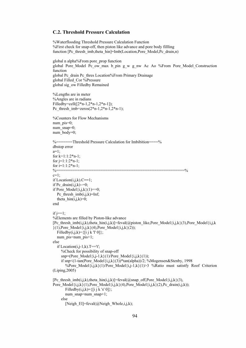
94
C.2. Threshold Pressure Calculation %Waterflooding Threshold Pressure Calculation Function %First check for snap-off, then piston like advance and pore body fillling function [Pc_thresh_imb,theta_hin]=Imb(Location,Pore_Model,Pc_drain,n) global n alpha%From pore_prop function global Pore_Model Pc_ow_max b_pin g_w g_nw Ac Ao %From Pore_Model_Construction function global Pc_drain Pc_thres Location%From Primary Drainage global Filled_Cor %Pressure global sig_ow Filledby Remained %Lengths are in meter %Angles are in radians Filledby=cell([2*n-1,2*n-1,2*n-1]); Pc_thresh_imb=zeros(2*n-1,2*n-1,2*n-1); %Counters for Flow Mechanisms num_pis=0; num_snap=0; num_body=0; %=======Threshold Pressure Calculation for Imbibition====% dbstop error a=1; for k=1:1:2*n-1; for j=1:1:2*n-1; for i=1:1:2*n-1; %=======================================================% c=1; if Location(i,j,k).C==1; if Pc_drain(i,j,k)~=0; if Pore_Modeli,j,k(1)==0; Pc_thresh_imb(i,j,k)=Inf; theta_hin(i,j,k)=0; end if j==1; %Elements are filled by Piston-like advance [Pc_thresh_imb(i,j,k),theta_hin(i,j,k)]=feval(@piston_like,Pore_Modeli,j,k(3),Pore_Modeli,j,k(1),Pore_Modeli,j,k(4),Pore_Modeli,j,k(2)); Filledby(i,j,k)=[i j k 'l' 0]; num_pis=num_pis+1; else if Location(i,j-1,k).T=='t'; %Check for possibility of snap-off snp=(Pore_Modeli,j-1,k(1)/Pore_Modeli,j,k(1)); if snp<(1-tan(Pore_Modeli,j,k(3))*tan(alpha))/2; %Mogensen&Stenby, 1998 %Pore_Modeli,j,k(1)/Pore_Modeli,j-1,k(1)>3 %Ratio must satistfy Roof Criterion (Liping,2005) [Pc_thresh_imb(i,j,k),theta_hin(i,j,k)]=feval(@snap_off,Pore_Modeli,j,k(3), Pore_Modeli,j,k(1),Pore_Modeli,j,k(4),Pore_Modeli,j,k(2),Pc_drain(i,j,k)); Filledby(i,j,k)=[i j k 's' 0]; num_snap=num_snap+1; else [Neigh_El]=feval(@Neigh_Whole,i,j,k);
95
num=1; for a=1:length(Neigh_El.x) %Determine # of filled neighbor elements if Pc_drain(Neigh_El.x(a),Neigh_El.y(a),Neigh_El.z(a))~=0; Neigh_Filling(num,1)=Neigh_El.x(a); Neigh_Filling(num,2)=Neigh_El.y(a); Neigh_Filling(num,3)=Neigh_El.z(a); c=c+1; num=num+1; end end c=c-1; if c==1 %Filling mechanism is either piston like or pore body filling [Pc_thresh.Piston(i,j,k),theta_h.Piston(i,j,k)]=feval(@piston_like,Pore_Modeli,j,k(3),Pore_Modeli,j,k(1),Pore_Modeli,j,k(4),Pore_Modeli,j,k(2)); [Pc_thresh.PoreFill(i,j,k),theta_h.PoreFill(i,j,k)]=feval(@pore_filling_imb, Pore_Modeli,j,k(3),Pore_Modeli,j,k(1),Pore_Modeli,j,k(4),Pore_Modeli,j,k(2),i,j,k,c,Neigh_Filling); if Pc_thresh.Piston(i,j,k)>Pc_thresh.PoreFill(i,j,k)
%Piston like mechanism is prefered Pc_thresh_imb(i,j,k)=Pc_thresh.Piston(i,j,k); theta_hin(i,j,k)=theta_h.Piston(i,j,k); Filledby(i,j,k)=[i j k 'l' 0]; num_pis=num_pis+1; else Pc_thresh_imb(i,j,k)=Pc_thresh.PoreFill(i,j,k); theta_hin(i,j,k)=theta_h.PoreFill(i,j,k); Filledby(i,j,k)=[i j k 'b' c]; end else %Filling mechanism is pore body filling with I_c [Pc_thresh_imb(i,j,k),theta_hin(i,j,k)]=feval(@pore_filling_imb,
Pore_Modeli,j,k(3),Pore_Modeli,j,k(1),Pore_Modeli,j,k(4), Pore_Modeli,j,k(2), i, j, k, c, Neigh_Filling);
Filledby(i,j,k)=[i j k 'b' c]; end end %End of if Pore_Modeli,j,k(1)/Pore_Modeli,j-2,k(1)>3 else [Neigh_El]=feval(@Neigh_Whole,i,j,k); num=1; for a=1:length(Neigh_El.x) %Determine # of filled neighbor elements if Pc_drain(Neigh_El.x(a),Neigh_El.y(a),Neigh_El.z(a))~=0; Neigh_Filling(num,1)=Neigh_El.x(a); Neigh_Filling(num,2)=Neigh_El.y(a); Neigh_Filling(num,3)=Neigh_El.z(a); c=c+1; num=num+1; end end c=c-1; disp(Neigh_Filling) if c==1 %Filling mechanism is either piston like or pore body filling [Pc_thresh.Piston(i,j,k),theta_h.Piston(i,j,k)]=feval(@piston_like,
Pore_Modeli,j,k(3),Pore_Modeli,j,k(1),Pore_Modeli,j,k(4), Pore_Modeli,j,k(2));
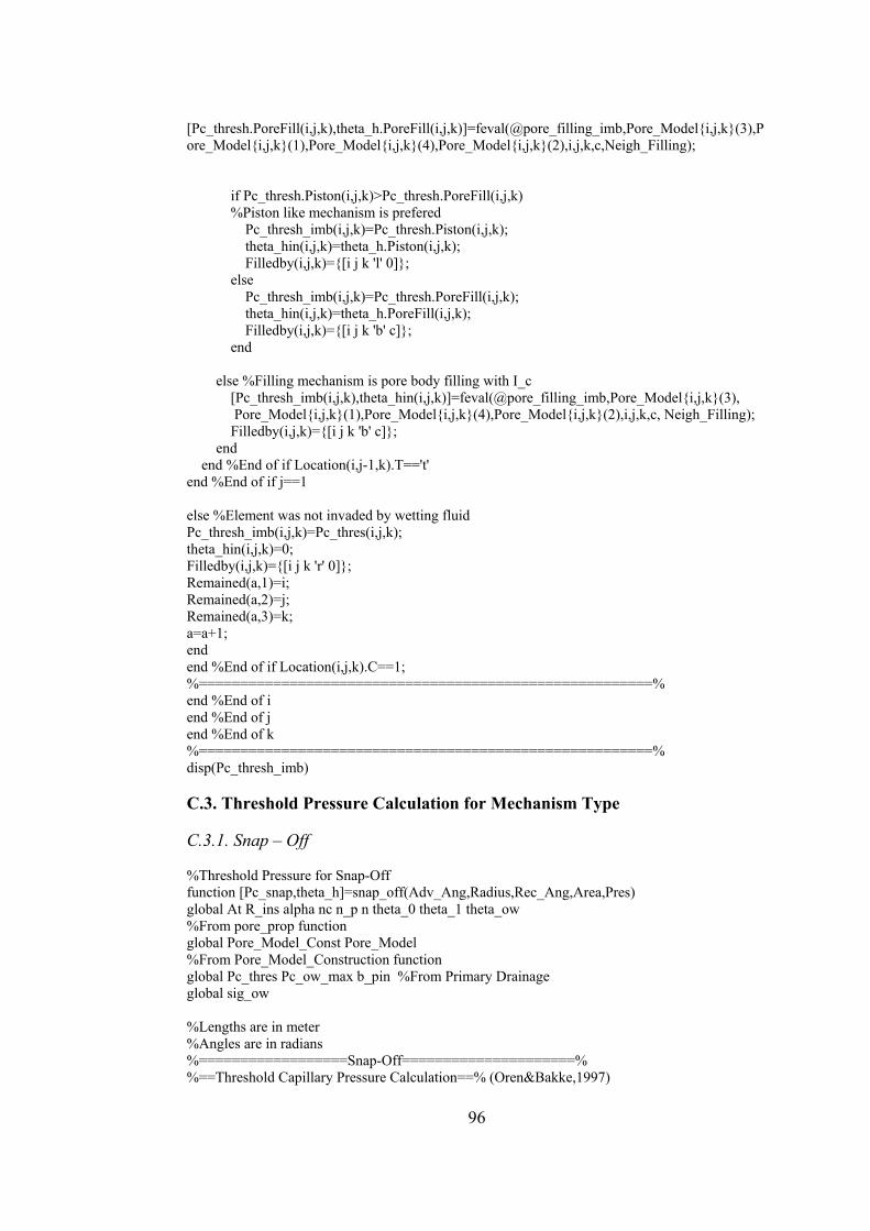
96
[Pc_thresh.PoreFill(i,j,k),theta_h.PoreFill(i,j,k)]=feval(@pore_filling_imb,Pore_Modeli,j,k(3),Pore_Modeli,j,k(1),Pore_Modeli,j,k(4),Pore_Modeli,j,k(2),i,j,k,c,Neigh_Filling); if Pc_thresh.Piston(i,j,k)>Pc_thresh.PoreFill(i,j,k) %Piston like mechanism is prefered Pc_thresh_imb(i,j,k)=Pc_thresh.Piston(i,j,k); theta_hin(i,j,k)=theta_h.Piston(i,j,k); Filledby(i,j,k)=[i j k 'l' 0]; else Pc_thresh_imb(i,j,k)=Pc_thresh.PoreFill(i,j,k); theta_hin(i,j,k)=theta_h.PoreFill(i,j,k); Filledby(i,j,k)=[i j k 'b' c]; end else %Filling mechanism is pore body filling with I_c [Pc_thresh_imb(i,j,k),theta_hin(i,j,k)]=feval(@pore_filling_imb,Pore_Modeli,j,k(3), Pore_Modeli,j,k(1),Pore_Modeli,j,k(4),Pore_Modeli,j,k(2),i,j,k,c, Neigh_Filling); Filledby(i,j,k)=[i j k 'b' c]; end end %End of if Location(i,j-1,k).T=='t' end %End of if j==1 else %Element was not invaded by wetting fluid Pc_thresh_imb(i,j,k)=Pc_thres(i,j,k); theta_hin(i,j,k)=0; Filledby(i,j,k)=[i j k 'r' 0]; Remained(a,1)=i; Remained(a,2)=j; Remained(a,3)=k; a=a+1; end end %End of if Location(i,j,k).C==1; %=======================================================% end %End of i end %End of j end %End of k %=======================================================% disp(Pc_thresh_imb) C.3. Threshold Pressure Calculation for Mechanism Type C.3.1. Snap – Off %Threshold Pressure for Snap-Off function [Pc_snap,theta_h]=snap_off(Adv_Ang,Radius,Rec_Ang,Area,Pres) global At R_ins alpha nc n_p n theta_0 theta_1 theta_ow %From pore_prop function global Pore_Model_Const Pore_Model %From Pore_Model_Construction function global Pc_thres Pc_ow_max b_pin %From Primary Drainage global sig_ow %Lengths are in meter %Angles are in radians %==================Snap-Off=====================% %==Threshold Capillary Pressure Calculation==% (Oren&Bakke,1997)
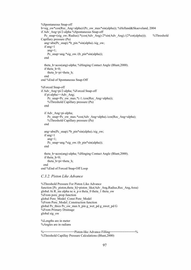
97
%Spontaneous Snap-off b=sig_ow*cos(Rec_Ang+alpha)/(Pc_ow_max*sin(alpha)); %Helland&Skaeveland, 2004 if Adv_Ang<pi/2-alpha %Spontaneous Snap-off Pc_snap=(sig_ow./Radius).*(cos(Adv_Ang)-2*sin(Adv_Ang)./(2*cot(alpha))); %Threshold Capillary pressure (Pa) ang=abs(Pc_snap).*b_pin.*sin(alpha)./sig_ow; if ang>1 ang=1; Pc_snap=ang.*sig_ow./(b_pin*sin(alpha)); end theta_h=acos(ang)-alpha; %Hinging Contact Angle (Blunt,2000). if theta_h<0; theta_h=pi+theta_h; end end %End of Spontaneous Snap-Off %Forced Snap-off if Adv_Ang>pi/2-alpha; %Forced Snap-off if pi-alpha>=Adv_Ang; Pc_snap=Pc_ow_max.*(-1./cos(Rec_Ang+alpha)); %Threshold Capillary pressure (Pa) end if Adv_Ang>pi-alpha; Pc_snap=Pc_ow_max.*cos(Adv_Ang+alpha)./cos(Rec_Ang+alpha); %Threshold Capillary pressure (Pa) end ang=abs(Pc_snap).*b_pin*sin(alpha)./sig_ow; if ang>1 ang=1; Pc_snap=ang.*sig_ow./(b_pin*sin(alpha)); end theta_h=acos(ang)-alpha; %Hinging Contact Angle (Blunt,2000). if theta_h<0; theta_h=pi+theta_h; end end %End of Forced Snap-Off Loop C.3.2. Piston Like Advance %Threshold Pressure For Piston Like Advance function [Pc_piston,theta_h]=piston_like(Adv_Ang,Radius,Rec_Ang,Area) global At R_ins alpha nc n_p n theta_0 theta_1 theta_ow %From pore_prop function global Pore_Model_Const Pore_Model %From Pore_Model_Construction function global Pc_thres Pc_ow_max b_pin g_wet_pd g_nwet_pd G %From Primary Drainage global sig_ow %Lengths are in meter %Angles are in radians %=================Piston-like Advance Filling==============% %Threshold Capillay Pressure Calculations (Blunt,2000)
98
theta_max=acos((-sin(alpha+Rec_Ang)*sin(alpha))./ ((Radius*Pc_ow_max * cos (alpha)/sig_ow)-cos(alpha+Rec_Ang))); %Blunt,2000
%=====Spontaneous Imbibition, Pc>0 (Blunt,2000)======% if Adv_Ang<=pi/2+alpha %theta_ow<=theta_max if Adv_Ang<=theta_max r=Radius; %Initial estimate for Effective Mean Radius of Curvature (m) Pc_thresh=sig_ow./r; %New value of Threshold Capillary Pressure (Pa) beta=asin(b_pin*sin(alpha)./r); %Angle A_eff=(Radius^2/(2*tan(alpha)))(r*b_pin*sin(alpha+beta)/2)+(r^2* beta/2) ; % Effective Area (m^2) omega_eff=((Radius./tan(alpha))-b_pin)*cos(Adv_Ang)+r.*beta; %Effective Perimeter (m) r_new=A_eff./omega_eff; %New value of Effective Mean Radius of Curvature (m) er=abs(r_new-r); %Error %Iteration Loop for Calculation of Threshold Capillary Pressure and Effective Mean Radius of Curvature (Blunt,2000) while er>0.001; %Error Control r=r_new; Pc_thresh=sig_ow./r; %New value of Threshold Capillary Pressure (Pa) beta=asin(b_pin*sin(alpha)./r); A_eff=(Radius^2/(2*tan(alpha)))(r*b_pin*sin(alpha+beta)/2)+(r^2*beta/2); omega_eff=((Radius./tan(alpha))-b_pin)*cos(Adv_Ang)+r.*beta; r_new=A_eff./omega_eff; %Calculates new value of Effective Mean Radius of Curvature (m) er_new=abs(r_new-r); er=er_new; end r=r_new; Pc_thresh=sig_ow./r; %Threshold Capillary Pressure for spontaneous imbibition (Pa) end %theta_ow>theta_max , Intermediate oil films are not created if Adv_Ang>theta_max Pc_thresh=2.*sig_ow.*cos(Adv_Ang)./Radius; %Threshold Capillary pressure (Pa) end end %End of Spontaneous Imbibition Loop %==Forced Imbibition , Pc<0, Intermediate oil films are created (Oren,1997)==% if Adv_Ang>pi/2+alpha %& Adv_Ang>theta_max %Threshold pressure calculation is same with primary drainage %Adv_Ang angle was used as advancing angle alpha_1=alpha; %Maximum value of corner half angle alpha_2=pi/4-alpha_1/2; %Minimum value of corner half angle G=(sin(2*alpha_1)/2).*(2.+(sin(2.*alpha_1)./sin(2.*alpha_2))).^-2; %Dimensionless shape factor D=pi*(1-Adv_Ang/(pi/3))+3.*sin(Adv_Ang).*cos(Adv_Ang)- (cos(Adv_Ang).^2)./(4*G); if D<0; D=0; end Fd=(1.+sqrt(1+4*G*D./(cos(Adv_Ang)).^2))./(1+2.*sqrt(pi*G));
99
Pc_thresh=(sig_ow.*(1+2*sqrt(pi*G)).*cos(Adv_Ang)./Radius).*Fd; %Threshold Capillary pressure (Pa) end %End of Forced Imbibition Loop %================================================% theta_h=acos(Pc_thresh*b_pin*sin(alpha)/sig_ow)-alpha; Pc_piston=Pc_thresh; C.3.3. Pore Body Filling %Pore Body Filling function [Pc_porefill,theta_h]=pore_filling_imb(Adv_Ang, Radius, Rec_Ang, Area, x, y, z, num_of, Filling_N) global alpha n nc%From pore_prop function global Pore_Model Location %From Pore_Model_Construction function global Pc_thres Pc_ow_max b_pin %From Primary Drainage global W_conduct %From Water Conductance function global sig_ow %=====================Pore Body Filling==================% %Threshold Capillay Pressure Calculations (Blunt,2000) theta_max=acos((-sin(alpha+Adv_Ang)*sin(alpha))./ ((Radius*Pc_ow_max*cos(alpha)/sig_ow)-cos(alpha+Adv_Ang))); %Blunt,2000 %====If theta_ow>theta_max, Invasion is similar to forced piston like imbibition====& if Adv_Ang>theta_max %Pc<0 and intermediate oil films are created %Threshold pressure is same with primary drainage alpha_1=alpha; %Maximum value of corner half angle alpha_2=pi/4-alpha_1/2; %Minimum value of corner half angle G=(sin(2*alpha_1)/2)*(2+(sin(2*alpha_1)/sin(2*alpha_2)))^-2; %Dimensionless shape factor D=pi*(1-Adv_Ang/(pi/3))+3*sin(Adv_Ang)* cos(Adv_Ang) (Adv_Ang)^2/(4*G); if D<0; D=0; end Fd=(1+sqrt(1+4*G*D/(cos(Adv_Ang))^2))/(1+2*sqrt(pi*G)); Pc_porefill=(sig_ow*(1+2*sqrt(pi*G))*cos(Adv_Ang)./Radius)*Fd; %Threshold Capillary pressure (Pa) end %End of Forced piston like imbibition %====If theta_ow<theta_max=======% if Adv_Ang<theta_max a=rand(1,num_of); g=rand(1,num_of); %Coefficient calculation for summation term coef=a(1,:).*g(1,:); sum=0; %Summation Term for counter=1:num_of
term=coef(1,counter)*Pore_ModelFilling_N(counter,1), Filling_N(counter,2),Filling_N(counter,3)(1);
sum=sum+term; end r_n=(1/cos(Adv_Ang))*(Radius+sum); %Mean Radius of Curvature Calculation Pc_porefill=2*sig_ow/r_n; %Threshold Capillary Pressure Calculation
100
end ang=abs(Pc_porefill)*b_pin*sin(alpha)/sig_ow; if ang>1 ang=1; Pc_snap=ang.*sig_ow./(b_pin*sin(alpha)); end theta_h=acos(ang)-alpha; %Hinging Contact Angle (Blunt,2000). if theta_h<0; theta_h=pi+theta_h; end end %End of pore filling loop %======================================================%
C.4. Conductance Calculation for Imbibition
%Capillary pressure and conductance calculations for Waterflooding (Imbibition Process) function[g_nwet,g_wet,Aw_total,Ao]=imbibition_conduct(M,Adv_Ang,theta_h,Rec_Ang,Pres, Area,Radius) global alpha n nc%From pore_prop function global Pore_Model Location %From Pore_Model_Construction function global Pc_thres Pc_ow_max b_pin %From Primary Drainage global W_conduct %From Water Conductance function global sig_ow if M=='s'; %==================Snap-Off=====================% %==Threshold Capillary Pressure Calculation==% (Oren&Bakke,1997) %Spontaneous Snap-off r_ow=sig_ow./Pres; %Interfacial radius of curvature (m) phi_3=(pi/2-alpha)*tan(alpha); %Conductance parameter f=1; %Boundary condition at fluid/fluid interface. (1 represents no-flow boundary) if Adv_Ang<pi/2-alpha %Spontaneous Snap-off %=Conductance Calculation (Blunt,2000)=% if theta_h>=Adv_Ang %Pore is completely filled by water g_wet=(pi*(sqrt(Area/pi)+Radius).^4)/128; %in m^4 %Pore is completely filled by water (m^4) (Wetting phase is water) g_nwet=0; %Non-Wetting phase is oil (m^4) Aw_total=Area; Ao=0; else %Pore is not filled by water. Remained same as at the end of Primary Drainage [g_nwet,g_wet,Aw_total,Ao]=feval(@conduct_drain,Pres,Rec_Ang,Area,Radius) ; end end %End of Spontaneous Snap-Off %Forced Snap-off if Adv_Ang>pi/2-alpha; %Forced Snap-off. Curvature is negative %==Conductance Calculation (Blunt,2000)==% if theta_h<Adv_Ang %Oil/Water/Solid Interface is pinned (Blunt,2000). Ac=nc.*r_ow.^2.*(cos(theta_h).*(cot(alpha).*cos(theta_h)-sin(theta_h))+theta_h+alpha-pi/2); %Area of Water in corners (m^2) if Ac<Area Ao=(Area-Ac); %Area of oil (m^2)

101
%Conductance Parameters phi_1=pi/2-alpha-theta_h; phi_2=cot(alpha)*cos(theta_h)-sin(theta_h); phi_3=(pi/2-alpha)*tan(alpha); g_wet=(Ac.^2.*(1-sin(alpha))^2.*(phi_2.*cos(theta_h)-phi_1)*phi_3^2)./ (12*nc*(sin(alpha))^2*(1-phi_3)^2.*(phi_2+f*phi_1).^2); %Wetting phase conductance. (Water is wetting phase) (m^4) g_nwet=(pi*(sqrt(Ao/pi)+Radius).^4)/128; %Conductance of water in center (m^4) else Ac=Area; Ao=0; g_wet=(pi*(sqrt(Area/pi)+Radius).^4)/128; %Conductance of water in center (m^4) g_nwet=0; end Aw_total=Ac; else %theta_h>= Adv_Ang; %Ac=nc.*r_ow.^2.*(cos(theta_h).*(cot(alpha).*cos(theta_h)-sin(theta_h))+theta_h+alpha-pi/2); %Area of Water in corners (m^2) Ac=nc.*r_ow.^2.*(cos(pi-Adv_Ang).*(cot(alpha).*cos(pi-Adv_Ang)-sin(pi-Adv_Ang))+ (pi-Adv_Ang)+alpha-pi/2); %Area of Oil layer + Area of water in corner (m^2) if Ac<Area Ao=(Area-Ac); %Area of oil (m^2) %Conductance Parameters phi_1=pi/2-alpha-theta_h; phi_2=cot(alpha)*cos(theta_h)-sin(theta_h); phi_3=(pi/2-alpha)*tan(alpha); g_wet=(Ac.^2.*(1-sin(alpha))^2.*(phi_2.*cos(theta_h)-phi_1)*phi_3^2)./ (12*nc*(sin(alpha))^2*(1-phi_3)^2.*(phi_2+f*phi_1).^2); %Wetting phase conductance. (Water is wetting phase) (m^4) g_nwet=(pi*(sqrt(Ao/pi)+Radius).^4)/128; %Conductance of water in center (m^4) else Ac=Area; Ao=0; g_wet=(pi*(sqrt(Area/pi)+Radius).^4)/128; %Conductance of water in center (m^4) g_nwet=0; end Aw_total=Ac; end end %End of Forced Snap-Off Loop if Adv_Ang==pi/2-alpha Pres=0; %Threshold Capillary pressure (Pa) (Oren&Bakke,1997) g_wet=(pi*(sqrt(Area/pi)+Radius).^4)/128; %in m^4 %Pore is completely filled by water (m^4) (Wetting phase is water) g_nwet=0; %Non-Wetting phase is oil (m^4) Aw_total=Area; Ao=0; end end %End of snap-off if M=='l' %=====================Piston-like Advance Filling==================% theta_max=acos((-sin(alpha+Rec_Ang)*sin(alpha))./((Radius*Pc_ow_max*cos(alpha)/sig_ow)- cos(alpha+Rec_Ang))); %Blunt,2000 %Threshold Capillay Pressure Calculations (Blunt,2000)
102
if Adv_Ang<=pi/2+alpha %theta_ow<=theta_max %==Conducatance Calculation (Blunt,2000)==% g_wet=(pi*(sqrt(Area/pi)+Radius).^4)/128; %in m^4 %Pore is completely filled by water (m^4) (Wetting phase is water) g_nwet=0; %Oil Conductance Ao=0; Aw_total=Area; end %End of Spontaneous Imbibition Loop %=====Forced Imbibition , Pc<0, Intermediate oil films are created (Blunt,2000)========% if Adv_Ang>=pi/2+alpha %& Adv_Ang>theta_max %Oil Films Stability Pressure (Oren&Bakke,1997) b2=2+cos(Adv_Ang)/sin(alpha); Pc_stab=-Pc_ow_max*(sin(alpha)/cos(Rec_Ang+alpha))*((1-b2^2)/(b2*cos(alpha)+sqrt(1- b2^2*(sin(alpha))^2))); %===Conductance Calculation (Blunt,2000)===% if abs(Pres)<Pc_stab %Oil films do not collapse ang=abs(Pres).*b_pin*sin(alpha)./sig_ow; if ang>1 ang=1; Pres=ang*sig_ow/(b_pin*sin(alpha)); end theta_h=acos(ang)-alpha; %Hinging Contact Angle (Blunt,2000). if theta_h<0; theta_h=pi+theta_h; end r_ow=sig_ow./Pres; %Interfacial radius of curvature (m) Aw_corner=nc.*r_ow.^2.*(cos(theta_h).*(cot(alpha).*cos(theta_h)-sin(theta_h))+theta_h+alpha-pi/2); %Area of Water in corners (m^2) if alpha+Adv_Ang==pi/2; %(From Piri&Blunt, 2005) Ac=(r_ow*cos(pi-Adv_Ang)/sin(alpha))^2*sin(alpha)*cos(alpha); else Ac= nc.*r_ow.^2.*(cos(pi-Adv_Ang).*(cot(alpha).*cos(pi-Adv_Ang)-sin(pi-Adv_Ang))+ pi-Adv_Ang+alpha-pi/2); %Area of Oil layer + Area of water in corner (m^2) end %Ac=nc.*r_ow.^2.*(cos(pi-Adv_Ang).*(cot(alpha).*cos(pi-Adv_Ang)-sin(pi-Adv_Ang)) +(pi-Adv_Ang)+alpha-pi/2); %Area of Oil layer + Area of water in corner (m^2) Ao=(Ac-Aw_corner); %Area of oil (m^2) Aw_center=Area-Ac; %Area of water in the pore center (m^2) Aw_total=Aw_corner+Aw_center; %Total area of wetting phase (water) (m^2) phi_3=(pi/2-alpha)*tan(alpha); %Conductance parameter f=1; %Boundary condition at fluid/fluid interface. (1 represents no-flow boundary) g_wet_corner=(Ac^2*tan(alpha)*(1-sin(alpha))^2*phi_3^2)/(12*nc*(sin(alpha))^2* (1-phi_3)*(1+f*phi_3)^2); %Conductance of water in corners (m^4) g_wet_center=(pi*(sqrt(Aw_center/pi)+Radius).^4)/128; %Conductance of water in center (m^4) g_wet= g_wet_corner+g_wet_center; %Total Water Conductance (m^4) f1=1; %Boundary condition at fluid/fluid interface. (1 represents no-flow boundary) f2=1; %Boundary condition at fluid/fluid interface. (1 represents no-flow boundary)
103
g_nwet=(Ao^3*(1-sin(alpha))^2*tan(alpha)*phi_3^2)/(12*nc*Ac*(sin(alpha))^2* (1-phi_3)*(1+f1*phi_3-(1-f2*phi_3)*sqrt(Aw_corner/Ac))^2); %Conductance of oil layer between water in center and water in corner (m^2) else %Pres>=Pc_stab, Oil films collapse g_wet=(pi*(sqrt(Area/pi)+Radius).^4)/128; %in m^4 %Pore is completely filled by water (m^4) (Wetting phase is water) g_nwet=0; %Oil Conductance Ao=0; Aw_total=Area; end end %End of Forced Imbibition Loop end %End of Piston-like if M=='b' %=====================Pore Body Filling==================% %====If theta_ow>theta_max, Invasion is similar to forced piston like imbibition====& theta_max=acos((-sin(alpha+Adv_Ang)*sin(alpha))./((Radius*Pc_ow_max*cos(alpha)/sig_ow)-cos(alpha+Adv_Ang))); %Blunt,2000 if Adv_Ang>theta_max %Pc<0 and intermediate oil films are created %Oil Films Stability Pressure (Oren&Bakke,1997) b2=2+cos(Adv_Ang)/sin(alpha); Pc_stab=-Pc_ow_max*(sin(alpha)/cos(Rec_Ang+alpha))*((1-b2^2)/(b2*cos(alpha)+ sqrt(1-b2^2*(sin(alpha))^2))); %===Conductance Calculation (Blunt,2000)===% if abs(Pres)<Pc_stab & Adv_Ang>=pi/2+alpha %Oil films do not collapse ang=(Pres)*b_pin*sin(alpha)/sig_ow; if ang>1 ang=1; Pres=ang*sig_ow/(b_pin*sin(alpha)); end theta_h=acos(ang)-alpha; %Hinging Contact Angle (Blunt,2000). if theta_h<0; theta_h=pi+theta_h; end r_ow=sig_ow./Pres; %Interfacial radius of curvature (m) Aw_corner=nc.*r_ow.^2.*(cos(theta_h).*(cot(alpha).*cos(theta_h)-sin(theta_h)) +theta_h+ alpha-pi/2); %Area of Water in corners (m^2) if alpha+Adv_Ang==pi/2; %(From Piri&Blunt, 2005) Ac=(r_ow*cos(pi-Adv_Ang)/sin(alpha))^2*sin(alpha)*cos(alpha); else Ac= nc.*r_ow.^2.*(cos(pi-Adv_Ang).*(cot(alpha).*cos(pi-Adv_Ang)-sin(pi-Adv_Ang))+ pi-Adv_Ang+alpha-pi/2); %Area of Oil layer + Area of water in corner (m^2) end Ao=Ac-Aw_corner; %Area of oil (m^2) Aw_center=Area-Ac; %Area of water in the pore center (m^2) Aw_total=Aw_corner+Aw_center; %Total area of wetting phase (water) (m^2) phi_3=(pi/2-alpha)*tan(alpha); %Conductance parameter f=1; %Boundary condition at fluid/fluid interface. (1 represents no-flow boundary) g_wet_corner=(Ac^2*tan(alpha)*(1-sin(alpha))^2*phi_3^2)/(12*nc*(sin(alpha))^2* (1-phi_3)*(1+f*phi_3)^2); %Conductance of water in corners (m^4)
104
g_wet_center=(pi*(sqrt(Aw_center/pi)+Radius).^4)/128; %Conductance of water in center (m^4) g_wet= g_wet_corner+g_wet_center; %Total Water Conductance (m^4) f1=1; %Boundary condition at fluid/fluid interface. (1 represents no-flow boundary) f2=1; %Boundary condition at fluid/fluid interface. (1 represents no-flow boundary) g_nwet=(Ao^3*(1-sin(alpha))^2*tan(alpha)*phi_3^2)/(12*nc*Ac*(sin(alpha))^2* (1-phi_3)*(1+f1*phi_3-(1-f2*phi_3)*sqrt(Aw_corner/Ac))^2); %Conductance of oil layer between water in center and water in corner (m^2) else %Pres>=Pc_stab, Oil films collapse g_wet=(pi*(sqrt(Area/pi)+Radius).^4)/128; %Pore is completely filled by water .Water spontenously fills pore. Water Conductance (m^4) g_nwet=0; %Oil Conductance Aw_total=Area; Ao=0; end end %====If theta_ow<theta_max=======% if Adv_Ang<theta_max Aw_total=Area; g_wet=pi*(sqrt(Aw_total/pi)+Radius).^4/128; Ao=0; g_nwet=0; end %End of pore filling loop end %End of Pore_Filling if M=='r' %Remained Same g_wet=pi*(sqrt(Area/pi)+Radius).^4/128; %Water Conductance (m^4) g_nwet=0; Aw_total=Area; Ao=0; end