Pore-to-continuum Multiscale Modeling of Two-phase Flow in

Louisiana State UniversityLSU Digital Commons

LSU Doctoral Dissertations Graduate School

2013

Pore-to-continuum Multiscale Modeling of Two-phase Flow in Porous MediaQiang ShengLouisiana State University and Agricultural and Mechanical College

Follow this and additional works at: https://digitalcommons.lsu.edu/gradschool_dissertations

Part of the Chemical Engineering Commons

This Dissertation is brought to you for free and open access by the Graduate School at LSU Digital Commons. It has been accepted for inclusion inLSU Doctoral Dissertations by an authorized graduate school editor of LSU Digital Commons. For more information, please [email protected].

Recommended CitationSheng, Qiang, "Pore-to-continuum Multiscale Modeling of Two-phase Flow in Porous Media" (2013). LSU Doctoral Dissertations.3790.https://digitalcommons.lsu.edu/gradschool_dissertations/3790

https://digitalcommons.lsu.edu?utm_source=digitalcommons.lsu.edu%2Fgradschool_dissertations%2F3790&utm_medium=PDF&utm_campaign=PDFCoverPages

https://digitalcommons.lsu.edu/gradschool_dissertations?utm_source=digitalcommons.lsu.edu%2Fgradschool_dissertations%2F3790&utm_medium=PDF&utm_campaign=PDFCoverPages

https://digitalcommons.lsu.edu/gradschool?utm_source=digitalcommons.lsu.edu%2Fgradschool_dissertations%2F3790&utm_medium=PDF&utm_campaign=PDFCoverPages

https://digitalcommons.lsu.edu/gradschool_dissertations?utm_source=digitalcommons.lsu.edu%2Fgradschool_dissertations%2F3790&utm_medium=PDF&utm_campaign=PDFCoverPages

http://network.bepress.com/hgg/discipline/240?utm_source=digitalcommons.lsu.edu%2Fgradschool_dissertations%2F3790&utm_medium=PDF&utm_campaign=PDFCoverPages

https://digitalcommons.lsu.edu/gradschool_dissertations/3790?utm_source=digitalcommons.lsu.edu%2Fgradschool_dissertations%2F3790&utm_medium=PDF&utm_campaign=PDFCoverPages

mailto:[email protected]

PORE-TO-CONTINUUM MULTISCALE MODELING OF TWO-PHASE FLOW IN POROUS

MEDIA

A Dissertation

Submitted to the Graduate Faculty of the

Louisiana State University and

Agricultural and Mechanical College

in partial fulfillment of the

requirements for the degree of

Doctor in Philosophy

in

The Department of Chemical Engineering

by

Qiang Sheng

B.S., Tianjin University, 2004

May 2013

ii

Acknowledgements

First and foremost, I would like to thank my advisor Dr. Karsten Thompson for giving

me a great opportunity to work on this project. He provided me with great guidance,

encouragement and support I needed in my graduate studies as well as the completion of this

dissertation. I would also like to thank Dr. Joanne Fredrich from BP for offering the subsurface

micro-tomography (microCT) data and financial support to my research. I would like to thank

Schlumberger for additional in-kind support. I want to thank my other advisory committee

members, Dr. Francisco Hung, Dr. Krishnaswamy Nandakumar, Dr. Joseph Siebenaller and Dr.

Clinton Willson for their time and valuable suggestions in my academic research.

I greatly appreciate the help from Dr. Peter Salino of BP for offering the experimental

relative permeability data. I also want to thank Dr. Tony Ladd from university of Florida for

offering Lattice Boltzmann results. My sincere thanks also go to Dr. Le Yan for his help in high

performance computation. I thank Dr. Kyungmin Ham from LSU CAMD for her help to obtain

another microCT data.

I would also like to thank my lab mates Pradeep, Nathan, Amin, Yijie, Tejaswini, Saade,

Tim, Dongxing, Lumeng, and Yin for their help and encouragement throughout my graduate

study. I thank the undergraduate student Ryan for his help in scientific visualization. I am greatly

appreciative of all the help from the supporting staff in Department of Chemical Engineering:

Paul Rodriguez, Darla Dao, Melanie McCandless, Melissa Fay, Danny Fontenot and Robert

Willis, and Andi Donmyer from Department of Petroleum Engineering.

Last but not the least, many thanks go to my parents and my wife Chai for their

unconditional love and support. I cannot imagine completing the graduate study and dissertation

iii

without their encouragement. My thanks also go to my good friend Rong for his support and

friendship throughout the six years of my graduate study.

iv

Table of Contents

Acknowledgements ......................................................................................................................... ii

List of Tables ............................................................................................................................... viii

List of Figures ................................................................................................................................ ix

Abstract ........................................................................................................................................ xiv

1. Introduction ................................................................................................................................. 1

2. Background and Literature Review ............................................................................................ 8

2.1. Pore-scale Modeling ............................................................................................................ 8

2.1.1. Rationale behind Pore-scale Modeling ........................................................................ 8

2.1.2. Physically Representative Network Models ................................................................ 9

2.1.3. Single-phase Network Models ................................................................................... 10

2.2. Two-phase Network Models ............................................................................................. 13

2.2.1. Qausi-static Models ................................................................................................... 13

2.2.2. Semi-dynamic Models ............................................................................................... 14

2.2.3. Dynamic Models Using the Washburn Equation ...................................................... 16

2.2.4. Dynamic Models that Solve the Two-phase Equations Simultaneously ................... 18

2.2.5. Steady-state Dynamic Network Models .................................................................... 19

2.2.6. Unified Dynamic Network Models............................................................................ 20

2.3. Macroscopic Properties ..................................................................................................... 21

2.3.1. Single-phase Properties ............................................................................................. 21

2.3.2. Two-phase Properties ................................................................................................ 23

2.4. Numerical Prediction of Relative Permeability ................................................................. 25

2.4.1. Quasi-static Network Method .................................................................................... 25

2.4.2. Unsteady-state Network Method ............................................................................... 26

2.4.3. Steady-state Network Method ................................................................................... 28

2.4.4. LBM or other CFD Methods ..................................................................................... 29

2.5. Pore-to-continuum Multiscale Models .............................................................................. 30

2.5.1. Boundary Coupling .................................................................................................... 32

2.5.2. Sequential Coupling ................................................................................................... 32

2.5.3. Concurrent Coupling.................................................................................................. 34

v

3. Single-phase Network Modeling and Validation ...................................................................... 40

3.1. Materials and Methods ...................................................................................................... 41

3.1.1. Porous Materials ........................................................................................................ 41

3.1.2. Single-phase Network Modeling ............................................................................... 43

3.1.3. Permeability Prediction using Network Modeling .................................................... 46

3.1.4. Network Model Validation ........................................................................................ 47

3.2. Results and Discussions .................................................................................................... 50

3.2.1. Permeability Comparison in a Computer-generated Sphere Packing ........................ 50

3.2.2. Pore-scale Flow Distribution Comparison ................................................................. 53

3.2.3. Permeability for Anisotropic Porous Media .............................................................. 54

4. A Unified Dynamic Network Algorithm for Two-phase Flow ................................................ 61

4.1. Methods and Materials ...................................................................................................... 61

4.1.1. Porous Materials ........................................................................................................ 61

4.1.2. Dynamic Two-phase Network Model........................................................................ 63

4.1.3. Relative Permeability Prediction ............................................................................... 76

4.2. Results and Discussions .................................................................................................... 77

4.2.1. Permeability and Characteristic Scale ....................................................................... 77

4.2.2. Periodic Steady-state Simulation ............................................................................... 77

4.2.3. Injection of Multiple Phases in Non-periodic Systems ............................................. 82

4.2.4. Periodic versus Non-periodic Steady-state Simulation ............................................. 95

5. Numerical Prediction of Relative Permeability ........................................................................ 97

5.1. Core Samples and Network Generation ............................................................................ 97

5.1.1. Core Samples ............................................................................................................. 97

5.1.2. MicroCT Imaging ...................................................................................................... 97

5.1.3. Network Generation ................................................................................................... 98

5.2. Network Modeling of Relative Permeability .................................................................. 100

5.2.1. Quasi-static Method (QS) ........................................................................................ 100

5.2.2. Unsteady-state Method during a Dynamic Displacement Process (USS) ............... 101

5.2.3. Steady-state Method Using a Periodic Network (SSP) ........................................... 101

5.2.4. Steady-state Method Using a Non-periodic Network (SSN) ................................... 103

5.2.5. Phase Saturation Distributions ................................................................................. 104

5.3. Results ............................................................................................................................. 105

5.3.1. Permeability and Characteristic Scale ..................................................................... 105

vi

5.3.2. Relative Permeability ............................................................................................... 106

5.4. Discussions ...................................................................................................................... 112

5.4.1. Relative Permeability Curves and Saturation Distribution ...................................... 112

5.4.2. Visual Interpretation ................................................................................................ 114

5.4.3. Comparison to Laboratory Data .............................................................................. 117

6. Dynamic Coupling of Pore-scale and Reservoir-scale Models .............................................. 119

6.1. Materials and Methods .................................................................................................... 119

6.1.1. Porous Materials ...................................................................................................... 119

6.1.2. Dynamic Two-phase Network Model...................................................................... 121

6.1.3. Relative Permeability Simulation ............................................................................ 123

6.1.4. Macroscopic Reservoir Model ................................................................................. 123

6.1.5. Coupled Multiscale Algorithm ................................................................................ 125

6.2. Results ............................................................................................................................. 128

6.2.1. Steady-state Relative Permeability Test .................................................................. 128

6.2.2. Rate Effect on Relative Permeability ....................................................................... 130

6.2.3. Concurrent Model with a Constant Injection Rate .................................................. 131

6.2.4. Concurrent Model with a Variable Injection Rate ................................................... 136

7. Conclusions and Recommendations ....................................................................................... 145

7.1. Conclusions ..................................................................................................................... 145

7.1.1. Single-phase Network Model .................................................................................. 145

7.1.2. Two-phase Network Model ..................................................................................... 146

7.1.3. Relative Permeability Prediction ............................................................................. 148

7.1.4. Multiscale Coupling ................................................................................................. 149

7.2. Recommendations ........................................................................................................... 151

7.2.1. Single-phase Network Model .................................................................................. 151

7.2.2. Two-phase Network Model ..................................................................................... 152

7.2.3. Relative Permeability Prediction ............................................................................. 153

7.2.4. Multiscale Coupling ................................................................................................. 154

References Cited ......................................................................................................................... 156

Appendix A. Table of Conductance Methods ............................................................................. 166

Appendix B. Numerical Prediction of Formation Factor ............................................................ 174

Appendix C. Numerical Prediction of Permeability Tensor ....................................................... 176

vii

Appendix D. Two-phase Reservoir Modeling and Validation ................................................... 177

Vita .............................................................................................................................................. 180

viii

List of Tables

Table 3-1: Networks parameters using different merging criteria ................................................ 51

Table 3-2: Permeability results using selected gij methods and three different networks ............ 52

Table 3-3: Average normalized residual (ANR) using selected gij methods and different merging

criteria ........................................................................................................................................... 53

Table 3-4: Permeability results using network model and FEM (permeability unit:10-6

cm2) ..... 56

Table 3-5: Permeability results using different merging criteria and conductance methods for the

stretched porous medium (permeability unit:10-6

cm2) ................................................................ 57

Table 3-6: Angles between eigenvectors and the unit vector of the coordinate system ............... 59

Table 3-7: Angles between eigenvectors and the unit vector of the coordinate system ............... 60

Table 4-1: Network specifications ................................................................................................ 62

Table 4-2: Fluid parameters .......................................................................................................... 62

Table 5-1: fluid properties and simulation time .......................................................................... 107

Table 5-2: Irreducible saturation using different network methods............................................ 112

Table 6-1: Network specifications .............................................................................................. 129

Table 6-2: Fluid parameters ........................................................................................................ 129

Table 6-3: Simulation specification in the reservoir model ........................................................ 131

Table A-1: Conductance methods ............................................................................................... 166

ix

List of Figures

Figure 3-1: a) Random sphere packing; b) Dolomite sample. ...................................................... 41

Figure 3-2: Image of the dolomite sample with the pore network model superimposed. ............ 42

Figure 3-3: Overlap between two inscribed pore bodies (Al-Raoush et al., 2003). ..................... 44

Figure 3-4: a) DT network; b) MDT1 network; c) MDT2 network for a computer-generated

sphere packing containing 100 spheres......................................................................................... 44

Figure 3-5: Three computer generated packings: 1) a random sphere packing containing 1,000

spheres; 2) a packing with 100% stretching in x direction (Only the coordinates are stretched,

and the particles remain the same size and spherical shape); 3) a laminated packing with large

spheres (0.115 cm radius) in the center, and small spheres (0.05 cm radius) on both sides......... 45

Figure 3-6: Geometric operations for constructing a stretched and rotated packing. ................... 45

Figure 3-7: LBM velocity integration in a typical pore throat of a computer-generated random

spheres packing ............................................................................................................................. 48

Figure 3-8: Velocity distribution comparison between LBM and network models using different

conductance methods and merging criteria a) DT gij 250; b) DT gij 260; c) MDT1 gij 250; d)

MDT1 gij 260; e) MDT2 gij 250; f) MDT2 gij 260 ....................................................................... 55

Figure 3-9: Least-square fits of the conductance formula gij=kGp with k=1.27 and p=2.57 ........ 56

Figure 4-1: a) Lattice network; b) sand network; c) sandstone network ...................................... 62

Figure 4-2: Schematics of various types of frontal displacement in the pore with coordination

number of z=4 (Lenormand et al., 1988): a) Throat filling; b) I0 for compressible non-wetting

phase; c) I1 for one connecting throat filled with non-wetting phase; d) I2 for two adjacent

connecting throats filled with non-wetting phase; e) I2 for two opposite connecting throats filled

with non-wetting phase; f) I3 for three connecting throats filled with non-wetting phase. .......... 65

Figure 4-3: Examples of local capillary pressure vs. saturation functions. .................................. 67

Figure 4-4: Examples of relative conductance vs. saturation functions. ...................................... 71

Figure 4-5: a) A 40×40 lattice network b) the lattice network is mirrored around a center plane 73

Figure 4-6: Permeability variation for subsamples of a) sandstone image; b) sand image .......... 78

Figure 4-7: Transient saturation and wetting-phase pressure profiles for individual pores 1001,

1002, 1003 at Sw,ave = 0.40 (sand network) ................................................................................... 79

Figure 4-8: Steady-state pressure distributions for wetting phase (red color) and non-wetting

phase (blue color) at Sw,ave = 0.35 (sand network) and capillary number Ca=2.32×10-4

. Non-

x

wetting pressures are only shown in the backbone pores where two phases flow simultaneously.

....................................................................................................................................................... 80

Figure 4-9: Relative permeability curve using periodic steady-state method (sand network) at

capillary number Ca=2.32×10-4

. At each saturation value, the phases were distributed uniformly

(the same saturation in each pore). ............................................................................................... 81

Figure 4-10: Saturation distributions at average Sw,ave =0.8 in a 100×100 lattice network. a) IC1,

uniform initial saturation; b) IC2, biased initial saturation distribution; c) steady-state saturation

distribution for IC1; d) steady-state saturation distribution for IC2. Simulations are run on a

200×100 periodic lattice network (by mirroring a 100×100 lattice network). Only the original

100×100 lattice network is used for saturation visualization........................................................ 83

Figure 4-11: Relative permeability curves using periodic steady-state simulations with different

initial conditions a) sand network; b) sandstone network ............................................................. 84

Figure 4-12: a) System saturation profile during a steady-state test using a sand network at

capillary number Ca=5.44×10-4

; b) fractional flow ratio curve using a sand network; c) relative

permeability curves using a sand network. Fractional flow ratios 0.00, 0.11, 0.28, 0.44, 0.88 and

1.00 were used. ............................................................................................................................. 86

Figure 4-13: Transient saturation and pressure profiles for individual pores at qw/qtol = 0.44 (sand

network) ........................................................................................................................................ 86

Figure 4-14: a) System saturation profile during a steady-state test (drainage and imbibition)

using a sandstone network; b) Relative permeability curves using a sand network (The black

curve shows relative permeability for a drainage process; the blue curve shows relative

permeability for an imbibition process; the red curve shows a scanning relative permeability

curve). Fractional flow ratios 0.88, 0.44, 0.28, 0.11, 0.00, 0.11, 0.28, 0.44, 0.88 and 1.00 were

used in a drainage and imbibition cycle. The scanning imbibition relative permeability curve was

acquired by starting to increase the fractional flow at saturation 0.67. ........................................ 87

Figure 4-15: Relative permeability curves without cut-off condition using a sandstone network

(The black curve shows relative permeability for a drainage process; the blue curve shows

relative permeability for an imbibition process) ........................................................................... 88

Figure 4-16: Drainage relative permeability curves at different capillary numbers: Ca =1.24×10-3

;

Ca =1.24×10-4

; Ca =1.24×10-5

using a sand network .................................................................... 90

Figure 4-17: Steady-state pressure distributions for wetting (red color) and non-wetting phase

(black color) for fractional flow (qw/qtol) 0.44 at different capillary numbers a) Ca=1.24×10-3

; b)

Ca=1.24×10-4

; c) Ca=1.24×10-5

(sand network). Non-wetting pressures are only shown in the

backbone pores where two phases flow simultaneously............................................................... 90

Figure 4-18: Saturation configurations at different viscosity ratios (M) and fractional flow ratio

(F= qw/qtol): a) F=0.0, M=0.1 at Sw=0.80; b) F=0.0, M=1 at Sw=0.80; c) F=0.0, M=30 at Sw=0.80;

d) F=0.5, M=0.1 at Sw=0.63; e) F=0.5, M=1 at Sw=0.63; f) F=0.5, M=30 at Sw=0.63. Red to

yellow colors denote the wetting phase; blue denotes the non-wetting phase. ............................. 92

xi

Figure 4-19: Saturation distributions at Sw,ave =0.8 using a sandstone sample for a) drainage

(F=0.0); b) steady-state flow (F=0.5). The network model saturations are mapped onto voxels

using an approximate method (Chapter 5). Red Color denotes the non-wetting phase; blue color

denotes the wetting phase. ............................................................................................................ 92

Figure 4-20: Drainage relative permeability curves using different resistance factors for non-

periodic steady-state simulations a) sandstone network; b) sand network ................................... 93

Figure 4-21: Drainage relative permeability curves using different inlet saturation distributions

for non-periodic steady-state simulations for a sandstone network. ............................................. 94

Figure 4-22: Relative permeability curves using both periodic steady-state simulation and non-

periodic steady-state simulation a) sandstone network; b) sand network ..................................... 96

Figure 5-1: a) Porosity and b) permeability variation for subsamples of the microCT image ... 105

Figure 5-2: Relative permeability curves using the quasi-static method .................................... 107

Figure 5-3: a) Average oil saturation and b) effective viscosity profiles during drainage ......... 110

Figure 5-4: a) Fractional flow ratio and b) relative permeability curves at the outlet ................ 110

Figure 5-5: a) Fractional flow and b) relative permeability curves using steady-state method .. 111

Figure 5-6: Bulk saturation during the steady-state test. ............................................................ 111

Figure 5-7: a) Fractional flow ratio and b) relative permeability curves using steady state

simulation. ................................................................................................................................... 112

Figure 5-8: Relative permeability curves using different methods ............................................. 114

Figure 5-9: Fluid distributions in slice 300 of the xy cross-section (orthogonal to the flow

direction) for a) steady-state periodic simulation and b) steady-state non-periodic simulation at

Sw=0.53 ....................................................................................................................................... 115


direction) for a) quasi-static simulation and b) steady-state non-periodic simulation at Sw=0.51

..................................................................................................................................................... 116

Figure 5-11: Fluid distributions in slice 300 of the yz cross-section for a) quasi-static simulation

and b) steady-state non-periodic simulation at Sw=0.51. Flow is from left to right in both images.

..................................................................................................................................................... 116

Figure 5-12: Experimental versus simulated USS relative permeability .................................... 117

Figure 6-1: Image of the sandstone data set with the pore network model superimposed (pores

shown as inscribed spheres and throats shown as line connections). ......................................... 120

xii

Figure 6-2: Ball-and-stick schematics of the two network models used in this study:

a) unconsolidated sand; b) sandstone. ......................................................................................... 120

Figure 6-3: Schematic illustration of the 1D continuum model with a network in the center of

gridblock i. Fractional flows are calculated at grid block boundaries and sent to the network

model as boundary conditions. Instantaneous relative permeability for gridblock i are estimated

from the network model and returned to the host gridblock. ...................................................... 128

Figure 6-4: Plots from the steady-state relative permeability test on the sandstone sample: a)

phase saturation versus pore-volumes injected; each plateau represents a steady-state relative

permeability data point; b) fractional flow ratio versus saturation; c) relative permeability curves.

..................................................................................................................................................... 129

Figure 6-5: Relative permeability curves at different flowrates: a) sandstone network;

b) unconsolidated sand network.................................................................................................. 130

Figure 6-6: a) Saturation comparison between the network and its associated gridblock for β=8

(cylindrical throat shape). The sandstone network was embedded in gridblock 10. b) Comparison

of the network and reservoir fractional flow curves for β=8. c) Saturation comparison between

the network and its associated gridblock β=65.02 (for equilateral triangular throat shape). d)

Comparison of the network and reservoir fractional flow curves for β=65.02. .......................... 132

Figure 6-7: a) Comparison of network vs. gridblock saturations for the unconsolidated sand.

b) Comparison of network versus reservoir fractional flow curves for the unconsolidated sand

network. ...................................................................................................................................... 135

Figure 6-8: Relative permeability comparisons: the black curve shows relative permeability

predicted using the network model as a stand-alone tool; the red curve shows relative

permeability determined from a coupled model with constant-rate displacement at Ca=10-1

. ... 135

Figure 6-9: Behavior of the concurrent multiscale model in a variable rate application using the

sandstone network: a) comparison of network saturation with host gridblock saturation; b)

steady-state relative permeability for two different rates (black) compared to actual relative

permeability values tracked by the coupled network during displacement (red). ...................... 137

Figure 6-10: Concurrent multiscale model with constant rate displacement (Ca=10-1

). Sandstone

networks were embedded in gridblocks 10, 15, and 20. a) Saturation and flowrate profiles; b)

relative permeability for two flowrates. Actual relative permeability values track the Ca=10-1

curve. ........................................................................................................................................... 138

Figure 6-11: Same plot as Figure 6-11a but for the variable rate simulation. Flowrate was

reduced by 0.5% every reservoir iteration. ................................................................................. 139

Figure 6-12: Concurrent multiscale model with variable rate displacement. a) Constant-rate

relative permeability profiles compared to the actual relative permeabilities tracked by the three

embedded networks; b) an enlarged view of the critical saturation range. ................................. 140

xiii

Figure 6-13: Saturation versus distance after 220 days in the waterflood simulation : comparison

of the sequential versus fully-coupled results. ............................................................................ 141

Figure 6-14: Saturation and flowrate profiles for the NAPL remediation simulation. Saturation

plots are for a gridblock in the concentrated spill zone (gridblock 50) and a gridblock

downstream of this zone (gridblock 70). Flowrate is lower for the first 800 days, then increased

by a factor of ten at day 800........................................................................................................ 141

Figure 6-15: a) Saturation versus time for gridblock 70 (downstream of the concentrated zone).

Comparison of two sequential coupling simulations with one concurrent simulation. The

sequential simulations were performed using different relative permeability curves

corresponding to the low and high injection rates. The concurrent simulation accounts for the

different injection rates automatically. Saturation for the concurrent plot is from the embedded

network. b) The two relative permeability curves (high and low rates) and relative permeability

tracked by the network model. .................................................................................................... 142

Figure 6-16: Saturation versus distance along the injection direction at day 1,000 for the NAPL

example. Comparison of sequential versus concurrent coupling. ............................................... 144

Figure 7-1: Saturation configurations at different viscosity ratios (M): a) M=0.003; b) M=10. Red

color denotes the wetting phase; blue color denotes the non-wetting phase. Simulations were

performed using a Level Set (LS) method in COMSOL.. .......................................................... 153

Figure D-1: Flow chart of a reservoir simulation process. For solving pressure, it follows the

process in right sub-flow diagram............................................................................................... 178

Figure D-2: Saturation distribution of Buckley-Leverett Problem ............................................. 178

Figure D-3: a) Simulation pressure distribution b) simulation saturation distribution c) analytical

pressure distribution d) analytical saturation distribution for 4 injectors in corners and 1 producer

in the center ................................................................................................................................. 179

xiv

Abstract

Pore-scale network modeling using 3D X-ray computed tomographic images (digital rock

technology) has become integral to both research and commercial simulations in recent years.

While this technology provides tremendous insight into pore-scale behavior, computational

methods for integrating the results into practical, continuum-scale models remain fairly

primitive. The general approach is to run pore-scale models and continuum models sequentially,

where macroscopic parameters are simulated using the pore-scale models and then used in the

continuum models as if they have been obtained from laboratory experiments. While a sequential

coupling approach is appealing in some cases, an inability to run the two models concurrently

(exchanging parameters and boundary conditions in real numerical time) will prevent using pore-

scale image-based modeling to its full potential.

In this work, an algorithm for direct coupling of a dynamic pore-network model for

multiphase flow with a traditional continuum-scale simulator is presented. The ability to run the

two models concurrently is made possible by a novel dynamic pore-network model that allows

simultaneous injection of immiscible fluids under either transient or steady-state conditions. The

dynamic network algorithm can simulate both drainage and imbibition. Consequently, the

network algorithm can be used to model a complete time-dependent injection process that

comprises a steady-state relative permeability test, and also allows for coupling to a continuum

model via exchange of information between the two models. Results also include the sensitivity

analysis of relative permeability to pore-level physics and simulation algorithms.

A concurrent multiscale modeling approach is presented. It allows the pore-scale

properties to evolve naturally during the simulated reservoir time step and provide a unique

method for reconciling the dramatically different time and length scales across the coupled

xv

models. The model is tested for examples associated with oil production and groundwater

transport in which relative permeability depends on flowrate, thus demonstrating a situation that

cannot be modeled using a traditional approach. This work is significant because it represents a

fundamental change in the way we might obtain continuum-scale parameters in a reservoir

simulation.

1

1. Introduction

Over the last several decades, fluid flow in porous media has garnered significant

attention of research and industry primarily due to oil and gas production and environmental

remediation (Dullien, 1992). Some important processes in oil and gas production that depend on

fluid flow in porous media, include flow towards wells from oil rich reservoirs, and fluid

injection such as water, surfactant or CO2 to increase the production from existing reservoirs

(Blunt et al., 2002). A better understanding of fluid flow in porous media also drives new

technologies in groundwater remediation (Celia et al., 1993). Additionally, numerous porous

media studies have been carried out on other areas, including flow through packed beds

(Thompson and Fogler, 1997), tissue engineering (Shanbhag et al., 2005), membrane filtration

(Long et al., 2010) and battery manufacturing (Mukherjee et al., 2010).

Numerical models are critical to describe porous media and predict fluid flow. The

general approach to modeling fluid flow in porous media is at the continuum scale, which solves

governing equations using average parameters. For example, reservoir simulation predicts oil

and gas production by solving two-phase conservation equations, which require macroscopic

parameters as the inputs. Macroscopic parameters, such as permeability and relative

permeability, are traditionally obtained from either laboratory experiments or empirical relations.

Laboratory experiments can be slow and costly. Empirical relations are not always general

enough for various geological rock types and lack a fundamental relationship to pore-scale

morphology and physics.

Pore-scale models provide an alternative approach to determine macroscopic parameters

by solving first-principles mass and momentum balance equations. They provide detailed pore-

2

scale information (e.g. saturation and pressure distributions). Flow properties at larger scales can

then be predicted using the pore-scale information. The ultimate goal of fluid flow simulation in

porous media is to quantify the physical processes at different scales, and to incorporate the

information into a single workflow.

Advances in 3D imaging techniques and advanced computation have led to an increase of

the use of digital rock workflow (Fredrich et al., 2006; Rassenfoss, 2011). A digital rock

workflow is usually comprised of five components: core recovery and preparation, imaging and

follow-up analysis, flow simulation, macroscopic properties prediction, and upscaling. Core

samples or segmented images are typically provided by collaborators, and the focus of this

research is on the last three components. A number of technical issues must be addressed in each

component.

First, an appropriate numerical approach should balance fundamental physics and

computational efficiency. The two most widely used pore-scale approaches are direct simulation

and network modeling. Direct simulation techniques such as the Lattice Boltzmann Method

(LBM) or other Computational Fluid Dynamics (CFD) techniques compute velocity and pressure

fields at the sub-pore scale. In contrast, network modeling imposes significant approximations to

both pore geometry and fluid mechanics, and is therefore a less rigorous approach. However, it

offers two potential advantages: 1. network models represent pore spaces by discrete networks of

pores and pore throats. By using a reduced data set (103-10

5 pores), network modeling is more

computationally efficient (i.e., a smaller computational problem for a similar-sized physical

simulation), which can be important for pushing the size of the physical domain that can be

modeled. 2. For two-phase flow, interfacial behavior can be incorporated into the pore-scale

equations that comprise the aforementioned flow approximations. This approach, while

3

approximate, obviates the need to capture problematic issues such as non-equilibrium jumps and

flow in thin films via fine-scale time and space discretization.

For two-phase network models, one has the choice of quasi-static simulation and

dynamic simulation. Quasi-static simulation is the most common method. However, this

approach only accounts for capillary forces, and has significant deficiencies at high capillary

numbers. Addressing this issue requires a dynamic network model, where the term dynamic as

used here means an algorithm that accounts for both viscous and capillary forces. The dynamic

two-phase network model has a fairly long history, although no single algorithm has emerged as

an accepted tool for porous media community. Most dynamic network models (Hughes and

Blunt, 2000; Singh and Mohanty, 2003; Nguyen et al., 2004) have been designed for

displacement processes (one phase to be displaced by another phase), which are not adequate to

describe complex flow conditions in a reservoir (Knudsen et al., 2002), such as concurrent or

counter-current flow. Other efforts (Constantinides and Payatakes, 1996; Knudsen et al., 2002)

incorporate periodic boundary condition to allow simultaneous injection of two phases.

However, this type of modeling is not capable of simulating saturation history since the average

system saturation is invariable in a periodic domain. Additionally, pore-scale dynamics in most

dynamic network models are usually described using criteria for a specific process (e.g.

displacement or steady-state flow), which inhibits the practicality of a unified network algorithm.

Second, the prediction ability of network methods should be improved with respect to

macroscopic properties. Multiphase macroscopic properties are especially important for

numerical simulation because of the experimental challenges, including the time associated with

laboratory measurements (Blunt, 2002). If an improved numerical prediction of macroscopic

4

properties is possible, network modeling will become important for core analysis and flow

characterization (Blunt, 2001).

Relative permeability is one of the most important multiphase macroscopic properties

because of its role in reservoir simulation. The most direct method for simulating relative

permeability is to perform fluid flow simulations that attempt to reproduce the analogous

laboratory experiment(s). Various numerical approaches have been used for relative permeability

prediction. Using a quasi-static network algorithm, relative permeability is modeled as a two-step

process: the pore-scale saturation is determined from a quasi-static displacement process, and the

relative-permeability is then calculated using independent single-phase network simulations

based on that particular phase distribution. Dynamic network models for displacement can be

used to simulate an unsteady-state relative permeability test. However, because of the small size

of the simulation domain (generally a few mm), it is not clear that a transient displacement

process is an appropriate description of relative permeability as used in reservoir scale models at

larger length and time scales. Performing relative-permeability simulations using steady-state

simulations has proved to be particularly difficult because inlet/outlet boundary conditions are

not known (i.e., for the cases in which more than one fluid is injected). However, if this problem

can be overcome, steady-state modeling of multiphase flow should provide a more direct way to

computationally back out relative permeability using the multiphase Darcy’s law. In one sense, it

is advantageous to have multiple algorithmic options (and this situation is not dissimilar to the

experimental situation where a range of techniques are used). However, a problem exists if the

algorithms produce different results, especially if the basis for these differences is not

understood.

5

Third, pore-scale information should be integrated into larger-scale continuum models

while accounting for both reservoir dynamics and the disparate time and length scales of the two

types of models (Patzek, 2001). Pore-scale models are usually millimeter order in size, and

seconds order in time, while continuum models are typically three orders of magnitude greater in

size and orders of magnitude larger in time. Upscaling from pore-scale models to a continuum-

scale model is not straightforward. A simple but limited multiscale approach is to predict

macroscopic parameters numerically in a pre-processing step, and then use the resulting

parameters in a continuum simulation in much the same way as if they had been obtained from a

physical laboratory experiment. In this approach, information is only passed in one direction

(from pore-scale model to continuum model).

In principle, information may be passed in both directions: Darcy velocities in each phase

are sent from the reservoir simulator to the network model to provide up-to-date boundary

conditions. Coupling in the opposite direction is via continuum properties such as relative

permeability, which are returned to the reservoir simulator. If this type of algorithm can be made

efficient, the potential benefits are dramatic. The most significant advantage is the ability to

eliminate traditional relative permeability curves. Instead, relative permeability values (as well as

capillary pressure if needed) for a gridblock come from its associated pore-scale model. This

approach has a number of major implications. 1. By providing real-time relative permeability

values, there is no need to parameterize relative permeability with saturation alone. Instead it can

vary with any parameters that the pore-scale model is capable of responding to (for instance

wettability, interfacial area, velocity, and more). 2. Because a network model marches in time

with its associated gridblock, it implicitly contains saturation history for that location and

therefore will automatically account for hysteretic effects. 3. This approach allows the relative

6

permeability data to remain accurate even if reservoir-scale conditions change, which might

affect the parameterized relative permeability curve. A simple example is changing Darcy

velocity due to injection or production rates from wells (under conditions where relative

permeability is rate dependent). More dramatic examples might be damage to absolute

permeability, changes in wettability, or unusual flow conditions such as countercurrent flow

during imbibition processes. A traditional approach (i.e., the use of relative permeability versus

phase saturation data) cannot account for these effects. However, with effective pore-to-

continuum coupling, the pore-scale model has the potential to respond to these effects and

communicate this information via updated values of the relevant parameters.

In this work, attempts have been made to address technical issues associated with two-

phase dynamic coupling. A uniform two-phase dynamic network model for simulating pore-scale

physics has been developed. The network model is evaluated in the context of prediction of

macroscopic properties such as permeability and relative permeability. The network model is

then used to develop a multiscale coupling algorithm, and to explore related numerical issues

that arise in the coupling process. The dissertation is organized as the following:

Chapter 2 presents the background of two-phase network modeling, macroscopic

property prediction, and multiscale simulation. In Chapter 3, a single-phase network model is

presented, and validated with direct simulation results. The effect of conductance is discussed

since it is the key parameter for both single- and multiphase network modeling. A novel

network approach is developed to predict the full permeability tensor for anisotropic porous

media. Chapter 4 presents a new unified two-phase dynamic network algorithm, which can be

run with one-phase injection (i.e. a displacement process) or two-phase simultaneous injection. It

includes a comprehensive sensitivity analysis of two-phase relative permeability on operational

7

parameters (e.g. injection rate, viscosity ratio), fluid mechanics (e.g. local saturation history, film

conductance), and numerical setups (e.g. initial conditions, boundary conditions). In Chapter 5,

different numerical approaches for relative permeability prediction are developed using

traditional quasi-static network algorithms as well as the new dynamic algorithm. The

differences between the models are discussed in the context of the physics that are captured by

the different algorithms and by direct examination of pore-scale saturation distributions. The

simulation results are also compared to experimental data. This is a first step toward interpreting

the underlying algorithmic differences and understanding the differences between experimental

techniques in the context of pore-scale behavior. In Chapter 6, a multi-scale algorithm is

developed to couple dynamic two-phase network models with a continuum reservoir model

concurrently for the first time. It shows how dynamic network models evolve with real time

reservoir conditions, and track local physics. The multiscale algorithm is demonstrated using

examples in both environmental and petroleum engineering. Chapter 7 summarizes the major

findings of the dissertation. Future work is also discussed.

8

2. Background and Literature Review

A review of the research that is relevant to pore-to-continuum multiscale modeling is

presented in the following subsections. Collectively, these studies suggest that pore-scale model

can be a viable research and commercial source for macroscopic properties, and an integral

component of the multiscale workflow for porous media.

2.1. Pore-scale Modeling

2.1.1. Rationale behind Pore-scale Modeling

A knowledge of pore-scale behavior is critical for understanding physical processes at

larger scales such as geological scale, reservoir scale and core scale. For example, the geological

storage of CO2 strongly depends on pore geometry and pore-scale capillary trapping mechanisms

(Benson and Cole, 2008; Knackstedt et al., 2010). Numerical modeling of the pore-scale

behavior is critical to understand fluid flow in porous media. Pore-scale modeling solves first-

principles governing equations at scales where the void structure can be resolved, thus allowing

insight into the fundamental physics.

Pore-scale modeling is instrumental in understanding fundamental flow phenomena in

porous media. Two different modeling approaches that can be used at the pore scale are network

modeling and direct simulation techniques. Direct simulation techniques such as Lattice

Boltzmann Method (LBM) or more traditional Computational Fluid Dynamics (CFD) techniques

discretize the pore space into numerical grids and solve the equations of motion. They represent

rigorous modeling techniques in terms of capturing porous structure and fluid dynamics.

Network modeling represents the same porous media using a much smaller data set, which

includes limited information about pore geometry (e.g. radius, volume) and topology information

9

(e.g. connectivity, orientation). This more approximate approach is more computationally

efficient, and therefore can be applied to larger domains and/or dynamic processes. Network

modeling will be the focus of this work.

2.1.2. Physically Representative Network Models

Quantitative network modeling using a realistic pore structure is attributed to Bryant et al.

(1993), who used the term “physically representative network models” to describe the rigorous

network generation process. Physically representative networks are created from realistic three

dimensional materials, which can include either computer-generated materials or 3D digital

images. The size of computer-generated networks is not limited by the size of the original image

(Idowu, 2009), and can be used to simulate multiscale porous media such as carbonate rocks

(Biswal et al., 2009). However, they use approximations to mimic complex geological processes

(Bakke and Øren, 1997). In contrast, 3D high-resolution images can characterize the

microstructure of a porous media in detail if the image resolution is adequate.

Transforming from digital image to a network structure is not a trivial procedure.

Different algorithms have been used: medial axis based method (Lindquist et al., 2000) or

maximum ball method (Silin et al., 2003). Thompson et al. (2008) developed a network

extraction algorithm by defining the locations of maximal inscribed spheres first using a

nonlinear optimization process. The center of each inscribed sphere is assigned as a pore

location. The void voxels are collected and assigned to the pore to which they belong. A search

for pore boundaries defines the pore-throat geometries and connectivity of the network. The

geometric properties used in the network are computed from the original image data, which

allows the network structure to be mapped with whatever level of detail necessary from the

original 3D images. It should be noted that there is no unique or correct network for most porous

materials. Some approaches assign void space into the pores only (Bakke and Øren, 1997;

10

Thompson et al., 2008), and some assign void space into the throats only (Bryant and Blunt,

1992; Bryant et al., 1993), while the others distribute void space into both pores and throats

(Silin et al., 2003; Dong and Blunt, 2009).

2.1.3. Single-phase Network Models

For single-phase network modeling, the fluid dynamics in a pore throat are characterized

by the throat conductance, which is defined using the following linear relationship between the

flow rate and pressure drop between two pores.

)( ji

ij

ij ppg

q

(2-1)

where pi and pj are pressures at pore i and j, respectively, qij is the flux between them, μ is the

viscosity, and gij is throat conductance. For lattice type networks, throat conductance can be

assigned from a statistical distribution (Li et al., 2006). For physically representative network

models, the issue of computing throat conductance is more important, because physically

representative network models are quantitative, and have few or no adjustable parameters.

Various conductance methods have been proposed over the years (Appendix A), but until

now there has been no quantitative information about which method better accounts for the

relevant pore geometry and captures fluid dynamics. Ewing and Gupta (1993) developed a one-

parameter model in which the throat conductance is a cubic function of throat radius. Their

approach ignored the effect of throat shape, and variation of throat radius along the flow axis.

Approximate conductance expressions have been derived by assuming ideal throat shapes. The

solution of fluid flow through a long cylindrical throat is given exactly by the Hagen-Poiseuille

equations. The cylindrical throat is characterized by its radius and length. To make use of a

Poiseuille type approach, one has a choice of the inscribed radius (Salter and Mohanty, 1982),

equivalent radius (Aker et al., 1998), effective radius (Bryant et al., 1993), hydraulic radius

11

(Dadvar and Sahimi, 2003), and CFD radius (Thompson and Fogler, 1997). The inscribed radius

is the radius of the largest circle that can be inscribed in throat cross section. The equivalent

radius is the radius of the equivalent circle with the same total cross section area. The effective

radius is defined as the arithmetic mean of the inscribed and equivalent radii. Hydraulic radius is

the ratio of throat area and the wetted perimeter. CFD radius is the radius from solving equation

of motion by direct simulation methods such as finite element method (FEM) or boundary

element method (BEM). Throat length, the second parameter in Hagen-Poiseuille expression, can

be estimated using the location of the two adjacent pores (Mani and Mohanty, 1999; Dadvar and

Sahimi, 2003). However, this approach tends to overestimate the throat length (if pore centers

are used). Bryant et al., (1993) shortened the throat length based on the geometrical analysis of

flow paths. Conductance formulas can also be derived using the approximations to torsion

problems with the same governing PDE (Sisavath et al., 2000). Using the Aissen approximation,

the conductance is estimated using the diameters of the throat inscribed circle and circumscribed

circle. Using the Saint-Venant approximation, the conductance is predicted using the throat

cross-sectional area and polar moment about the centroid.

Analytical conductance solutions have been used for non-circular throat shapes, such as

elliptical (Koplik et al., 1984; Seeburger and Nur, 1984), rectangular (Perrin et al., 2006),

triangular (Jia et al., 2008), and less familiar shapes such as the four cusp (Goode and

Ramakrishnan, 1993), and spherical bubbles (Blower, 2001). To compensate for non-circular

throat shape, correction factors have been introduced into Hagen-Poiseuille conductance

expression (Mortensen et al., 2005). Bakke and Øren (1997) used shape factor as the correction

factor to Hagen-Poiseuille expression. Shape factor was calculated based on the throat cross-

sectional area and wetted perimeter. Patzek and Silin (2001) used shape factor with cut-off

12

criteria: all throats with shape factors between those of equilateral triangle and the square can be

mapped onto squares, and those shape factors above square onto circles. Talabi (2008) estimated

shape factor using pore or throat volume, length, and grain surface area.

To account for the radius variation along the flow axis, Koplik (1982) modified the

Hagen-Poiseuille conductance by adding the contributions from throat entrance and exit. Several

studies (Roberts and Schwartz, 1985; Dias and Payatakes, 1986; Bryant et al., 1993; Liang et al.,

2000) divided a throat into small segments, estimated the conductance for each segment, and

used the harmonic mean of segment conductances for the total conductance. Ioannidis and

Chatzis (1993) calculated the conductance as a harmonic mean of the conductance of pores and

connecting throats. Throat conductance was calculated using a tabulated solution for rectangular

cross-sectional throat. Pore conductance was a cubic function of pore radius. Matthews et al.

(1993) used a similar approach, but assumed a cubic throat shape. Schlueter (1995) defined a

constriction factor to reflect the extent to which the pore radius varies along the path axis. Using

the constriction factor, he derived an analytical solution in which the variation of radius is

sinusoidal. Thompson et al. (1997) adjusted the conductance using a correction factor, by

comparing the conductance in a converging-diverging tube with the conductance in a parallel

tube. Bakke and Øren (1997) calculated the conductance using the harmonic mean of the

conductance among two pores and their connecting throat. Mogensen and Stenby (1998)

followed a similar method. Sisavath et al. (2001) derived a conductance formula using an

asymptotic series solution for sinusoidally varying throat. They found the asymptotic series

solution was more accurate than Hagen-Poiseuille solution for constricted throats. Lock et al.

(2002) applied a previous constriction factor (Schlueter, 1995) in an analytical solution for

sawtooth varying tube. Øren and Bakke (2003) used the effective pore and throat length to

13

calculate the conductance in two pores and their connecting throat. Dong and Blunt (2009) made

a similar correction, but used different weighting factors to calculate effective lengths.

Sholokhova et al. (2009) computed the total conductance using a weighted mean of the

conductances of two pores and their connecting throats. The weighting factors reflected the

contributions of pores and throats to the total conductance. They studied the sensitivity of

predicted macroscopic permeability to the weighting factors. They developed a hybrid pore-scale

model that used local LBM simulations to provide conductance values as the inputs to the

network model, and derived an empirical conductance formula based on LBM throat

conductance.

2.2. Two-phase Network Models

For immiscible two-phase flow, each phase exists in its own distinct pore space,

separated by fluid interfaces. The problem of multiphase flow is highly nonlinear with strong

coupling between the individual phase flowrates under many conditions. To gain fundamental

understanding of two-phase flow, many studies on network modeling have been conducted.

2.2.1 Quasi-static Models

Pore-network models for immiscible displacement can be divided into two categories:

quasi-static and dynamic models. Computationally, quasi-static models are equivalent to

invasion percolation processes. The algorithm simulates fluid displacement in the absence of

viscous effects. This type of algorithm also ignores the accumulation term. For an imposed

capillary pressure, the advance of displacement relies on the threshold capillary pressure. The

threshold capillary pressure for piston-like advance is given by:

t

likepistoncr

p cos2

, (2-2)

14

where is contact angle, σ is the interfacial tension, and rt is the throat radius. Quasi-static

models are the most efficient computationally and have been used extensively (Bryant and Blunt,

1992; Held and Celia, 2001; Valvatne and Blunt, 2004; Joekar-Niasar et al., 2008). They are

valid at zero capillary number (Ca = μnwl/σ), but cannot replicate the correct behavior at higher

capillary numbers.

2.2.2 Semi-dynamic Models

Semi-dynamic models solve the pressure field explicitly, but exclude capillary pressure in

the pressure equations. The governing equations can be cast as follows:

)(/

/,

ji

nww

nwwij

ij ppg

q

(2-3)

where μw/nw is the phase viscosity, and gij,w/nw is the phase conductance. Semi-dynamic models

assume that pore bodies and throats are filled with only one phase, and calculate the advance of

the displacement using a quasi-static approximation. They do not track the interface motion in

great detail, instead assuming the interface movement occurs instantaneously. As a result, semi-

dynamic models retain most of computational efficiency of quasi-static models.

Blunt and King (1991) performed drainage simulations in a computer-generated circular

network. They solved a single set of pressure equations, and ignored the local capillary pressure

in pore bodies. Phase conductance was calculated by comparing the pressure difference between

the two pores with the threshold capillary pressure of the connecting throat. Flow patterns were

characteristic of capillary fingering at low Ca, and experienced a transition from stable

displacement to viscous fingering for decreasing viscosity ratio (M = μnw/μw) at high Ca. Bakke

and Øren (1997) ran drainage simulations for computer-generated sandstone networks. They

included film flow in their model, and updated pore saturations by comparing the viscous

pressure gradients between the two pores with the throat threshold capillary pressure. Hughes

15

and Blunt (2000) developed a dynamic algorithm for imbibition in a square lattice network. They

assumed the non-wetting phase pressure gradient was negligible and only solved pressure

equations for the wetting phase. A fixed conductance was assigned for wetting films. They

selected displacement elements by comparing the pressure drop between two neighbor pores

with the throat threshold capillary pressure, which was calculated based on the preferred

mechanisms (frontal displacements, snap-off, and corporative filling). They later applied the

same model to simulate the imbibition process in fracture networks (Hughes and Blunt, 2001).

Yiotis et al. (2001) studied drainage using a dynamic network model. They coupled phase

changes in the pressure equations, and calculated the advance of the displacement using a quasi-

static approximation. They reported the effect of Ca on the saturation evolution. Nordhaug et al.

(2003) simulated drainage with circular-shaped pores in a dynamic model. They observed that

the fluid patterns switched from stable displacement to viscous fingering at decreasing viscosity

ratios. Nguyen et al. (2004) developed a dynamic network model for imbibition, and coupled the

pore-level dynamics such as film flow and snap-off in their model. They solved the pressure

equations only for the wetting phase, and computed the pore filling sequence based on the

competition between frontal displacement and snap-off. The thickness of wetting films was

calculated as a function of local capillary pressure. They studied the effect of Ca on fluid

distribution, relative permeability and residual saturation. Nguyen et al. (2006) applied the same

model in a computer-generated network, and studied the sensitivity of relative permeability and

residual saturation to Ca, wettability and pore structure. Idowu and Blunt (2010) extended a

previous dynamic network model for imbibition (Hughes and Blunt, 2000), and allowed the

wetting layer conductance to vary with pressure. The pressure equations for two phases were not

coupled, and solved independently. They studied the effects of Ca, M and wettability on fluid

16

distribution and saturation profile, and reproduced Buckley-Leverett profiles directly from pore-

scale modeling, thereby providing a bridge between the pore-scale and continuum-scale

transport. Hammond and Unsal (2012) developed a dynamic model based on a similar

displacement criterion used by Idowu and Blunt (2010). They ignored film swelling in their

model by assuming that the wetting film had a small effect on the conductance. They reported

fluid distributions at different M and Ca, and simulated a chemical enhanced oil recovery process

by reducing the interfacial tension or altering wettability.

2.2.3 Dynamic Models Using the Washburn Equation

A second class of dynamic models uses the Washburn equation to link viscous forces and

capillary forces:

)( cji

eff

ij

ij pppg

q

(2-4)

where pc is the throat threshold capillary pressure and μeff is the weighted average viscosities of

the two fluids. Washburn equation describes fluid flow in a capillary tube, but has been extended

to solve problems in porous media. In this type of model, pores have no capillary force or flow

resistance, and throats act as capillary barriers. Instead of solving two set of pressure equations

(one for each fluid), one can solve a single set of pressure equations for both fluids with different

viscosity such that, μeff depends on the interface position. This approach requires an interface

tracking method to identify where each fluid is, so that the correct value of the viscosity is

chosen.

Koplik and Lasseter (1985) used the Washburn approximation in a dynamic network

model for imbibition in which pressure was solved implicitly, and saturation was solved

explicitly. They studied the effect of Ca on transient fluid distributions when fluid viscosities of

both phases were equal. Dias and Payatakes (1986) developed a similar dynamic imbibition

17

model in a lattice network with converging-diverging throats, which implied that the capillary

pressure term in the Washburn equation depended on the interface position. They studied

transient displacement patterns at different M and Ca. Lenormand et al. (1988) developed a

dynamic drainage network model using the Washburn approximation, where μeff was calculated

by averaging two-phase viscosities, weighted by pore saturations. They studied the effects of Ca

and M on flow patterns. Mogensen and Stenby (1998) developed a dynamic network model for

imbibition that accounted for the competition between snap-off and frontal displacement by

comparing their minimum filling times. Film thickness was calculated a priori for each pore, and

was assumed to be constant through the simulation. They performed a sensitivity analysis of Ca,

wettability and pore structure on residual saturation. Aker et al. (1998) developed a dynamic

drainage algorithm in a lattice network with hour-glass shaped tubes, which allowed the local

capillary pressure vary along with the interface position. They neglected the film flow, and

calculated μeff by a sum of the amount of each fluid multiplied by their respective viscosities. The

temporal evolutions of the global pressure and three flow patterns (capillary fingering, viscous

fingering and stable displacement) were reported at different M and Ca. Dehle and Celia (1999)

developed a network model using the Washburn approximation. They allowed interfaces to

move over several pore-lengths within a time step. Singh and Mohanty (2003) developed a

dynamic network model for drainage. They included the effect of film flow in their model, and

studied the effect of Ca and M on fluid distribution. They demonstrated that dynamic capillary

pressures were higher than quasi-static capillary pressures for the same saturation values. Ferer et

al. (2003) developed a dynamic drainage network model, and coupled capillary forces using the

Washburn equation. They reported the effect of Ca and M on fluid distribution. Al-Gharbi and

Blunt (2005) developed a dynamic network model for drainage, and tracked the interface using

18

the equivalent hydraulic resistance of the fluids. Their model was then used to study the effects

of Ca and M on fluid distribution and fractional flow. Løvoll et al. (2005) extended Aker’s model

(1998) by including gravity forces. They demonstrated that flow patterns were governed by the

competition among viscous, capillary and gravity forces. Tørå et al. (2012) modified Aker’s

model (1998) by adding film flow, and reported a saturation exponent relationship and hysteresis

in the resistivity index.

2.2.4 Dynamic Models that Solve the Two-phase Equations Simultaneously

Dynamic models via the Washburn equation couple viscous forces and capillary forces in

a single set of equations. They use simplified rules to describe the pore-scale dynamics in an

approximate way. Those rules may violate a mass balance (Dahle and Celia, 1999), and require a

correction step to ensure that the change of saturation equal to the net flow of fluid through the

boundaries. To maintain mass balance for each fluid, a first-principles approach is to solve two-

phase mass conservation equations simultaneously, where the change of saturation for each fluid

is equal to the net flow of fluid in each pore integrated over a numerical timestep.

Thompson (2002) developed a dynamic network algorithm for imbibition in which the

two-phase conservation equations were solved simultaneously within each pore, helping to

reduce rule-based decisions in the algorithm. He defined the auxiliary functions such as local

capillary pressure and hydraulic conductance. Those relationships depended on local geometry

and saturation history. Currently, they must be estimated using relationships for simple

geometries; nonetheless, this approach remains the most direct approach for discretizing the

conservation equations for multiphase flow. Joekar-Niasar et al. (2010) used a similar approach

in which the two-phase conservation equations were solved simultaneously, and studied non-

equilibrium capillarity effects and the dynamics of two-phase flow.

19

2.2.5 Steady-state Dynamic Network Models

The aforementioned network models are designed for displacement processes.

Displacement algorithms create a large saturation change over very small (order-mm) linear

dimensions, which translates to an essentially infinite saturation gradient in the direction of flow

at the reservoir scale. The possibility of simulating steady-state two-phase flow is appealing

because the results can be interpreted directly using the multiphase Darcy equations (Dullien,

1992) and because steady-state multiphase flow may be more representative of the physical

processes that occur at the small length and time scales captured by pore-scale modeling. To

date, the difficulty in specifying appropriate boundary conditions has limited progress in this

area; periodic boundary conditions limit the types of networks that can be used and force

specification of an initial saturation condition at each saturation tested. At the same time, the

inability to impose known pore-scale boundary conditions for saturation has prevented the

development of non-periodic algorithms.

Constantinides and Payatakes (1996) developed a steady-state network model by

incorporating the Washburn-type equations (for immiscible displacement in a tube) into the

material balance. They simulated steady-state flow in a cubic lattice network with geometrically

identical inlet and outlet zones. Valavanides et al. (1998) coupled the same model with ganglion

population balance equations. Knudsen et al. (2002) developed a steady-state network model

with a periodic boundary condition in a 2D lattice based on Aker’s drainage model (1998). For

the case of two fluids with equal viscosity, they reported the effect of Ca on fluid regimes,

fractional flow ratio, and relative permeability. Knudsen and Hansen (2002) applied the same

model to derive a relationship between fractional flow ratio and global pressure drop. Ramstad

and Hansen (2006) used the model with a periodic boundary condition in a 2D lattice network.

They reported the temporal evolutions of the fluid distribution and global pressure, and found a

20

power-law distribution for large non-wetting phase clusters around a critical saturation in

capillary dominated regime. Ramstad et al. (2009) applied the same model in a 3D computer-

generated network, which was mirrored around the plane normal to the pressure gradient. They

reported that the steady-state saturation configuration was independent of initial distribution, and

found a power-law distribution for non-wetting phase clusters around a rate dependent critical

saturation in viscous dominated regime.

Periodic boundary conditions (with periodic or mirrored structures) provide an effective

way to study steady-state flow. However, simulations performed with periodic boundary

conditions are not capable of simulating saturation history and physically based hysteresis in

relative permeability. It limits the types of networks that can be used and forces specification of

an initial saturation condition because networks extracted from micro-tomography images

usually do not exhibit periodic structure.

2.2.6 Unified Dynamic Network Models

The concept of modeling drainage, imbibition and steady-state flow using a single

algorithm has long been viewed as appealing, but implementation has been slow. Two important

challenges are: 1. the boundary conditions are challenging to implement for a unified network

model because two-phase pressure and saturation are coupled through local capillary pressure.

2. Pore-scale dynamics are usually described using rules for a specific process such as drainage,

imbibition, or steady-state flow.

Aker et al. (1998) developed a dynamic model for drainage, and suggested that their

model could be extended to simulate imbibition by modifying the displacement rules. Dehle and

Celia (1999) developed a unified dynamic network model for drainage and imbibition, even

though the pore-level physics in their model is more relevant to drainage. Tørå et al. (2012)

21

extended Aker’s model (1998) to study imbibition and steady-state flow, by incorporating film

dynamics equations to account for wetting phase swelling and shrinking.

2.3. Macroscopic Properties

Porous media are characterized by macroscopic properties such as porosity, permeability,

formation factor, and relative permeability. Different experimental or empirical methods have

been developed to measure these macroscopic properties. Recently, digital rock technology has

developed as an alternative method to determine macroscopic properties under certain situations

by solving first-principles equations on digital images. Insights into the microscopic structure

help us to understand and interpret the properties of porous media, and digital rock technology

provides a tool to enhance the relationship between material structure and various macroscopic

properties.

2.3.1 Single-phase Properties

Porosity is the fraction of the pore or void space of the bulk volume. Porosity can be

divided into three categories: effective porosity (the connecting flow path), dead-end porosity

(connected only from one side and negligibly to transport), and isolated porosity (completely

disconnected from the flowing path and poorly connected micro-porosity). Experimental

methods for porosity measurement include the density method, optical method, wetting fluid

imbibition, mercury injection and gas expansion (Dullien, 1992). Using digital rock technology,

total porosity can be estimated directly from image analysis, while effective porosity can be

predicted by computing pore connectivity.

Permeability is defined by Darcy’s law, and dictates that flow rate increases linearly with

the applied pressure gradient. For isotropic porous media, the pressure gradient is always aligned

with the Darcy velocity. The permeability can vary depending on the direction of measurement

22

in anisotropic porous media, which require a permeability tensor to fully characterize the

permeability.

j

iij

pA

Qk

(2-5)

Permeability is usually measured using continuum-scale methods: formation testing and

core measurement (Anderson et al., 1994). Using digital rock technology, prediction of

permeability is performed by reproducing the analogous core measurement(s). Isotropic

permeability is calculated by imposing a pressure gradient in the x, y, or z direction. For

anisotropic porous materials, a novel technique has been developed in this work to determine the

full permeability tensors, by imposing simulations in three independent directions (Appendix C).

Formation factor is the ratio of the resistivity of a porous sample saturated with a

conducting fluid to the resistivity of that fluid. Formation factor is always greater than unity,

which indicates the solid surface of porous media is insulating.

w

F

(2-6)

At the pore scale, the electric potential field is determined by solving electrical current

conservation equation. Resistivity is then given by:

AIL

EE OI (2-7)

where σ is the resistivity, EI and Eo are electric potential at the inlet and outlet, respectively, I is

the electric flux between them, A is the cross-sectional area, and L is the length of the domain.

More details about resistivity and formation factor prediction can be found in Appendix B.

23

2.3.2 Two-phase Properties

Two-phase properties are more challenging to measure because of the interaction of two

phases, and complex behavior associated with wettability. Phase saturation is defined as the

fraction of total pore volume occupied by that specific fluid phase. Generally, saturation is

defined for wetting phase. Irreducible phase saturation is used to indicate the phase saturation at

which that phase becomes immobile (and therefore cannot be further removed by flow).

Capillary pressure is defined as the difference between the non-wetting phase pressure

and wetting phase pressure across an interface. Experimental measurements of capillary pressure

include the steady-state method and dynamic displacement method (Dullien, 1992). For the

displacement method, the capillary pressure is equal to the pressure difference between the inlet

and the outlet. For steady-state method, the capillary pressure is equal to the pressure difference

between the non-wetting phase and wetting phase at the inlet, which can be calculated using the

Young-Laplace equation:

rppp wnwc

cos2 (2-8)

At the continuum scale, a global capillary pressure is defined using a statistical average

taken over the void space. Recent studies (Hassanizadeh et al., 1993; Joekar-Niasar et al., 2010)

indicate that capillary pressure is not only a function of saturation, but also a function of

parameters such as interfacial area. At the pore scale, a local capillary pressure can be derived as

a function of local pore geometry, contact angle, and on the degree of saturation for ideal pore

geometries (Thompson, 2002; Joekar-Niasar et al., 2010).

Relative permeability is defined using multi-phase Darcy’s law for two-phase

simultaneous flow through the porous media. It is based on the assumption that the relative

permeability at certain saturation is independent of the phase pressure gradients.

24

i

i

rii p

kkv

(2-9)

where kri is the relative permeability for phase i, vi is the velocity for phase i, μi is the viscosity

for phase i, k is absolute permeability. Experimental approaches for relative permeability include

the steady-state method and dynamic displacement method (Dullien, 1992). In a dynamic

displacement method, one phase is injected to displace the other phase. Relative permeability

values are recovered from the outlet data, based on Buckley-Leverett theory. In a steady-state

method, two phases are injected simultaneously. Steady state is reached when constant saturation

and pressure drop are reached across the sample. No consensus exists as to what is the most

appropriate relative permeability measurement method because there is no clear experimental

evidence that a shock front is created and maintained (unsteady-state) or if a gradual change in

fractional flow occurs (steady-state) in a reservoir. In some systems, the resultant relative

permeabilities are nearly identical but in others, significant differences are observed (Schneider

et al., 1970; Peters et al., 1987).

Moreover, experimental studies show that relative permeability is not only a function of

saturation, but also of parameters such as capillary number (Avraam and Payatakes, 1999),

viscosity ratio (Lefebvre, 1973), contact angle (Owens and Archer, 1971), surface tension

(Bardon and Longeron, 1980), and saturation history (Talash, 1976). Clearly, a better

understanding of how these parameters affect relative permeability is a fundamental requirement

for accurate oil recovery prediction.

25

2.4. Numerical Prediction of Relative Permeability1

2.4.1. Quasi-static Network Method

Traditionally, relative permeability simulations using network models are performed in a

two-step process. In the first step, a quasi-static displacement is performed to a prescribed

capillary pressure. This displacement produces a distribution of fluids in the pore space, and this

distribution is used in an independent single-phase flow simulation that is normalized by the

(simulated) single-phase permeability to obtain a relative permeability.

Quasi-static models have been used in numerous past studies, which have examined a

wide range of physical behavior and employed various algorithmic advances to improve the

physics being captured by the simulations. Jerauld and Salter (1990) showed that the non-wetting

phase relative permeability primarily depends on the saturation in the backbone fraction. Blunt et

al. (1992) modified the quasi-static displacement process to account for flow with and without

trapping of a phase. For the relative permeability part of the calculation, O'Carroll and Sorbie

(1993) derived analytic expressions for the relative permeability using a quasi-static model.

Goode and Ramakrishnan (1993) found there was a lubrication effect in which the non-wetting

phase relative permeability could exceed unity at low wetting phase saturations, and which was

sensitive to the viscosity ratio. Relative permeabilities have been predicted and compared to

laboratory results for unconsolidated rock (Fenwick and Blunt 1998) and consolidated rock

(Blunt, 1997; Dillard et al., 2000). Fischer and Celia (1999) used measured capillary pressure-

saturation data to adjust lattice topology. Other authors made similar adjustments to control pore-

size distribution (Dillard et al. 2000; Laroche and Vizika, 2005; Jia et al. 2005). Other factors

that influence relative permeability have been modeled, including wall roughness (Blunt and

1 Section 2.4 is originally presented in SPE ATCE Conference in Oct 2011, Denver, CO.

26

King, 1992; Laroche and Vizika, 2005), flow rate (Blunt and King, 1992), contact angle (Blunt,

1997), and interfacial area (Joekar-Niasar et al., 2008).

A second generation of network models was created from the pore space in three-

dimensional structures such as sphere packings (Bryant and Blunt, 1992) and computer-

generated geologic materials (Bakke and Øren, 1997). Quasi-static relative permeability models

have been applied to these networks to study factors such as the effect of pore structure and

wettability (Bryant and Blunt, 1992; Bakke and Øren, 1997; Øren et al., 1998; Blunt et al., 2002;

Valvatne and Blunt, 2004; Jackson et al., 2005). Because these studies were applied to specific

3D structures rather than statistically equivalent lattice networks, these models can be thought of

as precursors of the image-based models being used today. Image-based networks are derived

directly from microCT and other 3D digital images. These types of network models have been

used for quasi-static relative permeability calculations in materials such as Fontainebleau

sandstone (Lindquist and Venkatarangan, 1999; Arns et al., 2003; Mahmud et al., 2007),

Bentheimer sandstone (Patzek, 2001), and carbonates (Al-Kharusi and Blunt, 2008). Arns et al.

(2003) observed a tendency to overestimate the wetting-phase relative permeability, and

attributed this to either a large coordination number or an insufficiently large network. They

suggested that the representative volume for single-phase properties might not be large enough to

produce meaningful estimates of relative permeabilities, and also showed that relative

permeabilities were significantly affected by network topology for a drainage process.

2.4.2. Unsteady-state Network Method

Unsteady-state methods are common experimentally, and in principle the same

procedures can be simulated using pore-scale models. Because simulations reveal the internal

saturation distribution, one potentially has more flexibility in what data can be used to calculate

relative permeability, as compared to core-scale experiments.

27

Hughes and Blunt (2000) used a rule-based dynamic imbibition algorithm in a square

lattice to fill pores (similar to a quasi-static model). However, they considered viscous forces in

the wetting phase by assigning a constant conductance for the wetting films. They divided the

network into thin regions (five pores in the flow direction) and calculated relative permeability in

each region. Singh and Mohanty (2003) developed a rule-based dynamic network model in a 3D

lattice network. To avoid solving the two-phase equations explicitly, they developed a heuristic

scheme to account for viscous forces in the wetting phase. Drainage relative permeabilities were

computed by applying the two-phase Darcy’s law to subsections of the network, averaging the

non-wetting phase flow rate since it varied along the length in the displacement direction. They

found relative permeability depended linearly on saturation at high capillary numbers and non-

linearly at low capillary numbers. Al-Gharbi and Blunt (2005) employed a dynamic network

model in a relatively small 2D lattice network. They computed the average saturation and

relative permeability in a four-pore-length section in the middle of the network. Nguyen et al.

(2006) developed a dynamic imbibition model using a network with 12,349 pores reconstructed

from Berea sandstone. They considered pressure gradients in wetting films but ignored viscous

gradients in the bulk fluid. They solved pressure fields separately in the water and oil sub-

networks and determined relative permeability using multi-phase Darcy’s law. Increasing flow

rate suppressed snap-off and resulted in relative permeability curves and residual saturations that

compared favorably with measured data for Berea sandstone. They also found that the rate

sensitivity was high for large pore-throat aspect ratios and low for small aspect ratios.

Tsakiroglou (2012) developed a multi-scale network type algorithm that could be applied to

large length scales (10 cm). They employed a dynamic model by solving the Washburn-type

28

equations and used non-wetting phase and wetting-phase outlet flow rates along with computed

pressure differences to calculate relative permeability from the multiphase Darcy equation.

These and other unsteady-state network simulations used the multiphase Darcy’s law to

calculate relative permeability. However, as shown in experiment (Jones and Roszelle, 1978) and

network simulation results (Singh and Mohanty, 2003), flow rates are not constant along the flow

direction. Hence, the question of whether Darcy’s Law (which is based on steady-state flow) can

be used effectively with displacement simulations needs further investigation.

2.4.3. Steady-state Network Method

Steady-state methods are the most closely aligned to multiphase Darcy’s equation, as all

parameters in Darcy’s equation are specified or measured directly from the network model (or

lab experiment). For modeling, detailed information such as internal saturation and pressure

distribution can also be recovered from the simulations. However, only a few studies exist

detailing steady-state network methods, due largely to the hurdle of accommodating the

simultaneous injection of two phases.

Constantinides and Payatakes (1996) simulated steady-state flow in a 30×20×5 lattice

network with geometrically identical inlet and outlet zones. They imposed periodicity in the flow

direction including allowing ganglia to move across the periodic boundaries, and solved for

pressure in every node by incorporating the Washburn-type equations (for immiscible

displacement in a tube) into the material balance. They calculated transient relative permeability

using Darcy’s law and obtained steady-state relative permeability by averaging the transient

values over a sufficiently long time. In the original paper (Constantinides and Payatakes, 1996),

the effects of capillary number and viscosity ratio on relative permeability were studied, while

Valavanides et al. (1998) added ganglion population balance equations. Knudsen et al. (2002)

studied the dynamics of two-phase immiscible bulk flow under steady-state conditions in a

29

20×40 square lattice of cylindrical tubes. Their model included periodic flow conditions, solved

for pressure and velocity using the Washburn equation, and maintained constant flow by

updating the applied pressure at every time step. Relative permeability was obtained using

multiphase Darcy’s law. Knudsen and Hansen (2002) used the same model to derive a

relationship between fractional flow ratio and global pressure drop. Ramstad et al. (2009) applied

the model to a Berea sandstone network with 12,349 pores by mirroring the network in the flow

direction. In their model, film flow was neglected and piston-like flow was assumed in the pores

by using the Washburn equation. Pressure and flow rates were computed using network

conservation equations, but relative permeability was not studied.

Challenges in developing a network model that can be used for steady-state relative

permeability simulation include: 1. to minimize rule-based algorithms as much as possible; and

2. allow for the incorporation of boundary conditions that reflect behavior in the reservoir and/or

in laboratory tests (depending on how the model is to be used). Thompson (2002) and Joekar-

Niasar et al. (2010) present an algorithm in which the conservation equations are applied to both

phases independently and are coupled through pore-scale capillary pressure and hydraulic

conductance, both of which are functions of local saturation. This approach can be used for

steady-state relative permeability simulation by adding boundary conditions to allow

simultaneous injection of two phases.

2.4.4. LBM or other CFD Methods

Although CFD modeling for two-phase flow simulation is not the focus of this work, it is

worth briefly mentioning this technique because the challenges associated with implementing

boundary/initial conditions are similar (to the steady-state periodic method) and because

comparisons between CFD and network results can be used to provide insights into the validity

of the underlying models. Li et al. (2005) performed two-phase LBM simulations on a 64×64×32

30

periodic lattice. They simulated concurrent flow by adding body forces for both phases. The non-

wetting phase was transported as disconnected blobs at high capillary numbers. They found that

relative permeabilities for both phases were increasing functions of capillary number, although

for higher capillary numbers (Ca >10-3

) the relative permeabilities were nearly constant. Ramstad

et al. (2009) performed two-phase LBM simulations on 1283 and 256

3 voxel domains using an

image from Bentheimer sandstone. They randomly distributed the fluid phases inside the void

space according to an initial target saturation and used both unsteady-state and steady-state

simulations to compute relative permeability. For the steady-state case, they applied periodic

boundary conditions, but phases crossed the boundaries freely. For the unsteady-state case, they

also applied periodic boundary conditions, but wetting fluid that exited the model was changed

to non-wetting fluid that was re-injected at the inlet face. They found that increasing capillary

number had minor effects on the wetting phase relative permeability but a strong effect on the

non-wetting phase relative permeability, especially at high saturation. Boek (2010) extracted an

800×800×630-voxel image from a sample of Bentheimer sandstone. Relative permeability was

computed using a 1283 sub section of this data set. The initial condition was a uniform saturation

distribution. Relative permeability was computed by applying body forces on oil or water or both

phases.

In the future, it is likely that other CFD-type algorithms will be used in addition to LBM.

For example, Silin and Patzek (2009) predicted relative permeability from images by solving the

Stokes equation for the velocity field using a finite difference method. Voxels in the digital

image were used as the numerical grid.

2.5. Pore-to-continuum Multiscale Models

The use of direct numerical simulation such as the LBM and approximate techniques

such as network modeling for pore-scale modeling have become commonplace in the last fifteen

31

years, largely because of the complementary technology, microtomography imaging. Together,

these tools have fostered rapid advances in image-based modeling. If modeling is performed on

sufficiently large domains, continuum parameters such as permeability can be obtained from the

flow simulations just as with a laboratory flow experiment. Generally, this approach is not

viewed as a replacement for experimental tests, but rather a complementary tool. Image-based

modeling has certain advantages (for instance the ability to perform an unlimited number of tests

on a sample). However, it also has many limitations, including whether the relevant physics can

be accurately captured by the pore-scale models and issues related to scale (numerical resolution,

image resolution, and physical size of the digital domains).

The most straightforward technique for upscaling pore-scale results is to perform pore-

scale simulations beforehand, and then to tabulate the results for subsequent use in continuum-

scale equations or models. This approach mimics the traditional laboratory approach and is

trivial to implement from a numerical standpoint because information is passed in only one

direction (from the pore to continuum scale). However, it does not take full advantage of the

benefits of multiscale modeling described in the introduction.

Upscaling in the continuum domain has been studied extensively, resulting in techniques

such as the multi-grid method (Durlofsky et al., 2007; Aarnes et al., 2007). This and similar

approaches are designed to allow models to operate over multiple continuum scales, and aid in

simulating multiscale physical and chemical phenomena such as water coning near a gas well or

hydrodynamic dispersion of chemical species in groundwater. While certain upscaling issues are

similar, pore-to-continuum multiscale modeling has certain unique problems that must be

addressed (Scheibe et al., 2007; E et al., 2007).

32

2.5.1. Boundary Coupling

For the sake of discussion, we divide pore-to-continuum multiscale techniques into two

categories: boundary coupling and hierarchical coupling. Boundary coupling links network

models with adjacent continuum regions at an interface between the two. Balhoff et al. (2007)

coupled a pore network model to a lower-permeability continuum region by matching the flux at

a shared interface. They demonstrated that both pore-scale heterogeneity and the resistance in the

low-permeability region affect the near-interface flow distribution in the continuum region,

making it essential to match flux and pressure at the coupling boundary. Subsequently,

Balhoff et al. (2008) developed a more general approach that couples pore-scale network models

to other adjacent pore-scale or continuum-scale models using a mortar method. This approach

demands a weaker flux match at the interface than the earlier technique but has a more flexible

formulation. Boundary coupling techniques work well for joining adjacent regions, but they are

not designed to upscale information across multiple length scales at the same location.

2.5.2. Sequential Coupling

A second class of multiscale modeling is hierarchical coupling, which links pore-scale

and continuum-scale models in the same region (e.g., from an embedded network model to the

continuum gridblock in which it resides). This technique must address large disparities in both

length and time scales (Patzek, 2001), and can require both numerical coupling and upscaling. A

simple but limited hierarchical approach is sequential coupling, where rock properties or

transport parameters such as permeability, relative permeability, or capillary pressure are

simulated in a pre-processing step and then used in a reservoir simulation in much the same way

as if they had been obtained from a physical laboratory experiment. Blunt et al. (2002) showed

that the assignment of relative permeability based on network modeling gives significantly

different predictions of oil recovery compared to using traditional empirical relative permeability

33

models, which implies sequential coupling could improve the predictive power of reservoir

models. Jackson et al. (2003) used the same coupled model to predict oil recovery for different

wettabilities. White et al. (2006) developed a multiscale model for simulating single-phase flow

through porous media. The pore space was discretized into smaller domains. LBM was used to

calculate micro-scale velocity distributions and permeability at the pore scale for each sub-

domain, and the results were then transmitted to a continuum model via tabular or empirical

permeability relationships as one would do with laboratory data. Lichtner and Kang (2007)

developed a multiscale model to study reactive flow. Pore-scale transport equations were solved

using LBM at the pore scale, and the results were upscaled through simple volume averaging at

slow reaction rate and fit into a multiscale continuum model. Rhodes et al. (2008) studied

particle transport at four different scales: pore, core, gridblock and field. At the pore scale,

transport was simulated using a network model. Transport properties were then upscaled to the

larger scales using transit time distribution functions. They argued that pore-scale or gridblock-

scale heterogeneity delayed transport and increased breakthrough times by up to an order of

magnitude compared to those predicted using a traditional advection and dispersion model. Chen

et al. (2010) developed a multiscale LBM simulation: pore-scale LBM was used to estimate

permeability after colloid deposition, and estimated permeability distribution was used in a

second LBM model to simulate flow at the continuum scale. Tsakiroglou et al. (2012) developed

a multiscale network type algorithm. They estimated capillary pressure and relative permeability

functions using a quasi-static network model and fed the information as the input to a

macroscopic simulator as part of an analysis of the axial distribution of water saturation and

pressure across a column-scale soil sample. Sun et al. (2011) studied the effect of sub-domain

size on the accuracy of a multiscale method, which couples LBM with a continuum model.

34

2.5.3. Concurrent Coupling

The aforementioned sequential coupling techniques offer the potential to replace or

augment coreflood experiments with numerical simulations. However, they do not exploit the

most powerful aspect of pore-scale to continuum-scale coupling, which is the ability of the pore-

scale model to march forward in time with the reservoir simulator, providing “just-in-time”

continuum-scale parameters needed at the larger scale. We will refer this approach to as

concurrent coupling in this work.

To date, few studies have been published in the area of concurrent coupling. Heiba et al.

(1986) coupled a statistical network model for two-phase flow with a reservoir-scale finite

element solver. Relative permeability was calculated using percolation theory. They argued that

this approach provides more accurate and reliable prediction of relative permeability and

capillary pressure in two-phase displacements compared to empirical correlations, but with a

factor of 100 computational penalty compared to conventional reservoir simulation because of

the computational cost that was required to predict capillary pressure and relative permeabilities

that appear in the continuum equations. Celia et al. (1993) proposed a concurrent multiscale

simulation framework to couple a quasi-static network model with a continuum model. The idea

consisted of a two-way exchange process: network simulators located in the center of selected

blocks in the continuum model providing bulk properties to these blocks. In turn, the continuum

simulator provides boundary conditions (in the form of fluid pressures) for the network model. A

concurrent multiscale simulation strategy using LBM was also proposed by Van den Akker

(2010). Neither of these latter two models was implemented at the time that they were proposed

because of numerical limitations. Chu et al. (2012a) developed a single-phase multiscale

algorithm that couples network models to continuum-scale models, in which network properties

such as throat conductance are nonlinear functions of the macroscopic properties at a much

35

larger scale. They used the multiscale algorithm to model non-Darcy flow. Chu et al. (2012b)

integrated a dynamic pore-scale model for immiscible displacement with a reservoir model for

multiphase flow. They decoupled the pressure and saturation computations by using two separate

sets of networks: networks placed at gridblock boundaries were used for pressure calculation

while separate networks were placed along the displacement front (where the saturation gradient

is larger) to be used for saturation updates.

Concurrent coupling methods that have been developed to date have employed a number

of simplifications that allow the multiscale coupling to be performed and/or to improve

numerical efficiency. However, these simplifications have corresponding restrictions associated

with the physics of flow, including the following:

1. Quasi-static models are limited to zero-capillary-number behavior (viscous effects are

negligible). In addition, because viscosity is absent from the model (in the displacement part of

the algorithm), time is not a parameter in the model. Hence, the quasi-static assumption

precludes modeling viscous behavior or any time-dependent effects (which in turn eliminates

many of the reservoir processes that would benefit most from multiscale, multiphase modeling).

2. Most multiphase algorithms model immiscible displacement (rather than more general

multiphase flow processes). These pore-scale simulations create a large saturation change over

very small (order-mm) linear dimensions, which translates to an essentially infinite saturation

gradient in the direction of flow at the reservoir scale. Consequently, both the magnitude of the

saturation gradient and the spatial distribution of phases (which dictates relative permeability)

are inconsistent with what would be expected in a reservoir.

3. For finite-difference or finite-volume algorithms (at the continuum scale), two possible

mappings of pore-scale models onto the continuum grid are to (i) associate a pore-scale model

36

with the interior of a gridblock or (ii) place pore-scale models at gridblock boundaries. The latter

approach allows for a simpler numerical approach if it is run such that a pore-scale model on the

+x boundary (for instance) is operated using only a dP/dx pressure gradient. However, this

approach implies that the continuum grid is aligned with the principal directions for the

permeability tensor, which restricts generality of the algorithm. (In fact, the ability to detect

micro-scale anisotropy and transmit this information to the continuum scale is a good example of

the value of pore-to-continuum upscaling.)

4. As discussed below, no explicit equation links phase saturation in a pore-scale model

with the saturation in its home gridblock, at least in a natural formulation derived directly from

the conservation equations. If these values are forced to be equal (for instance by a forced update

to the pore-scale saturation at each timestep so that it matches the current gridblock saturation),

this procedure in effect erases information associated with saturation history that is otherwise

contained implicitly in the pore-scale model.

The issue of viscous versus quasi-static multiphase modeling is not unique to the

multiscale framework, and it has a fairly long history in network modeling. Multiphase network

models that account for viscous effects (termed dynamic algorithms) remain tricky to implement

even after 25 years of research, and no single algorithm has emerged as an accepted tool for

practical modeling. Thompson (2002) developed a model in which the two-phase conservation

equations are solved simultaneously within each pore. Joekar-Niasar et al. (2010) used the

aforementioned approach in which the phase conservation equations are solved simultaneously.

This latter model was also used for the coupled model by Chu et al. (2012b) mentioned above.

Using the LBM simulations for multiphase flow automatically addresses the quasi-static

problem. However, while LBM simulations are more rigorous than network models, they are less

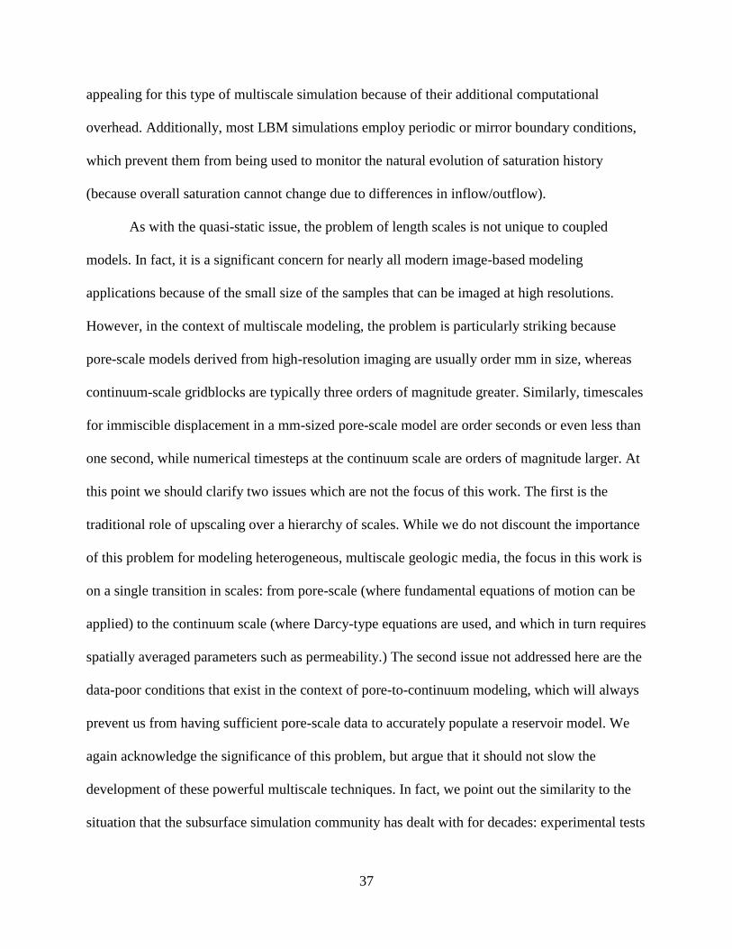
37

appealing for this type of multiscale simulation because of their additional computational

overhead. Additionally, most LBM simulations employ periodic or mirror boundary conditions,

which prevent them from being used to monitor the natural evolution of saturation history

(because overall saturation cannot change due to differences in inflow/outflow).

As with the quasi-static issue, the problem of length scales is not unique to coupled

models. In fact, it is a significant concern for nearly all modern image-based modeling

applications because of the small size of the samples that can be imaged at high resolutions.

However, in the context of multiscale modeling, the problem is particularly striking because

pore-scale models derived from high-resolution imaging are usually order mm in size, whereas

continuum-scale gridblocks are typically three orders of magnitude greater. Similarly, timescales

for immiscible displacement in a mm-sized pore-scale model are order seconds or even less than

one second, while numerical timesteps at the continuum scale are orders of magnitude larger. At

this point we should clarify two issues which are not the focus of this work. The first is the

traditional role of upscaling over a hierarchy of scales. While we do not discount the importance

of this problem for modeling heterogeneous, multiscale geologic media, the focus in this work is

on a single transition in scales: from pore-scale (where fundamental equations of motion can be

applied) to the continuum scale (where Darcy-type equations are used, and which in turn requires

spatially averaged parameters such as permeability.) The second issue not addressed here are the

data-poor conditions that exist in the context of pore-to-continuum modeling, which will always

prevent us from having sufficient pore-scale data to accurately populate a reservoir model. We

again acknowledge the significance of this problem, but argue that it should not slow the

development of these powerful multiscale techniques. In fact, we point out the similarity to the

situation that the subsurface simulation community has dealt with for decades: experimental tests

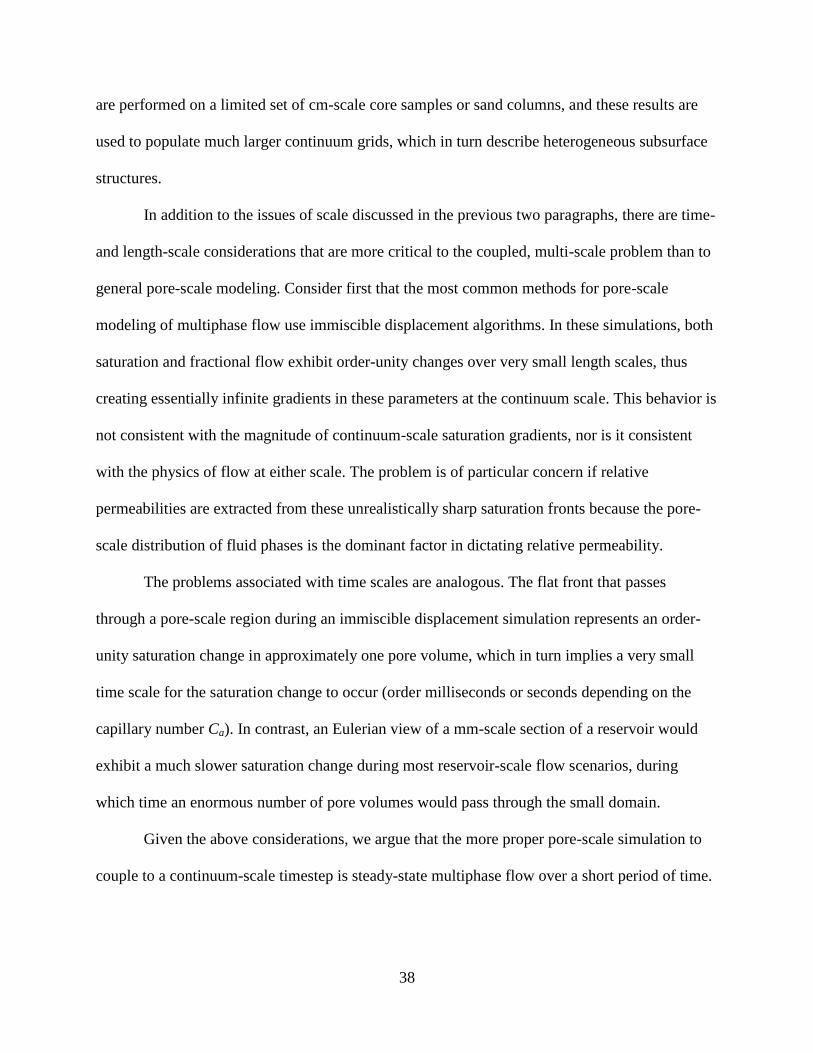
38

are performed on a limited set of cm-scale core samples or sand columns, and these results are

used to populate much larger continuum grids, which in turn describe heterogeneous subsurface

structures.

In addition to the issues of scale discussed in the previous two paragraphs, there are time-

and length-scale considerations that are more critical to the coupled, multi-scale problem than to

general pore-scale modeling. Consider first that the most common methods for pore-scale

modeling of multiphase flow use immiscible displacement algorithms. In these simulations, both

saturation and fractional flow exhibit order-unity changes over very small length scales, thus

creating essentially infinite gradients in these parameters at the continuum scale. This behavior is

not consistent with the magnitude of continuum-scale saturation gradients, nor is it consistent

with the physics of flow at either scale. The problem is of particular concern if relative

permeabilities are extracted from these unrealistically sharp saturation fronts because the pore-

scale distribution of fluid phases is the dominant factor in dictating relative permeability.

The problems associated with time scales are analogous. The flat front that passes

through a pore-scale region during an immiscible displacement simulation represents an order-

unity saturation change in approximately one pore volume, which in turn implies a very small

time scale for the saturation change to occur (order milliseconds or seconds depending on the

capillary number Ca). In contrast, an Eulerian view of a mm-scale section of a reservoir would

exhibit a much slower saturation change during most reservoir-scale flow scenarios, during

which time an enormous number of pore volumes would pass through the small domain.

Given the above considerations, we argue that the more proper pore-scale simulation to

couple to a continuum-scale timestep is steady-state multiphase flow over a short period of time.

39

Generally this would be at a new saturation that has evolved to match the current continuum-

scale timestep.

40

3. Single-phase Network Modeling and Validation

Single-phase flow in porous media is one of the most well-studied areas in porous media

research. Single-phase flow has traditionally been studied using experimental measurements.

However, experimental methods are limited by two factors: first, the details of pore-scale flow

patterns are rarely known from experiments, especially for complex 3D geometry. Second,

measurement of 3D permeability tensor in complex porous media is time consuming, and there is

a lack of quantitative interpretation in terms of pore structure (Dullien, 1992). Using direct

simulations for single-phase flow automatically addresses the first issue. However, direct

simulations are not possible for large porous samples with engineering significance because of

their computational overhead. Network modeling is more computationally efficient than direct

simulations, but is less rigorous because of its approximations to both pore structure and fluid

mechanics. If the validity of network models can be improved, network modeling should provide

a fast method to computationally predict macroscopic properties.

In this chapter, we compare the pore-scale flow distribution using various conductance

methods in network simulation with that from a more rigorous LBM simulation in a small

computer-generated random packing material. The permeability tensor and principal flow

direction for anisotropic porous media are determined using a novel network approach, and

validated using a prototype sphere packing with a known structure. Finally, anisotropy is

predicted for real rock samples.

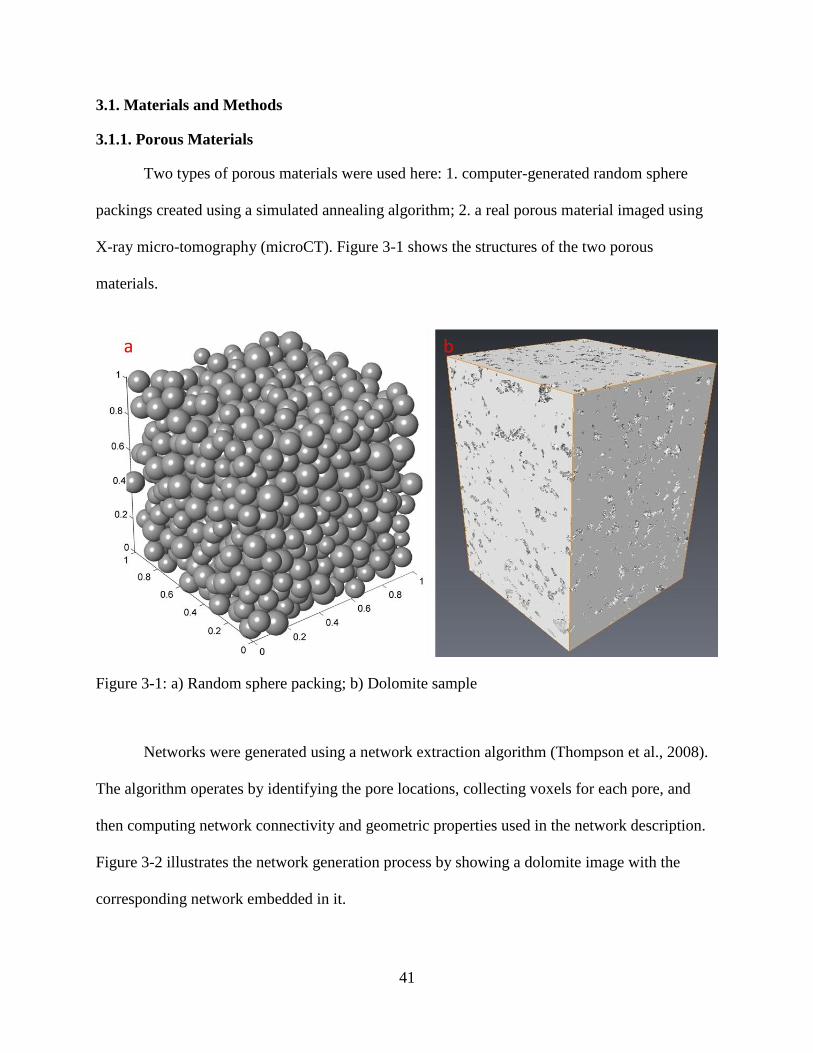
41

3.1. Materials and Methods

3.1.1. Porous Materials

Two types of porous materials were used here: 1. computer-generated random sphere

packings created using a simulated annealing algorithm; 2. a real porous material imaged using

X-ray micro-tomography (microCT). Figure 3-1 shows the structures of the two porous

materials.

Figure 3-1: a) Random sphere packing; b) Dolomite sample

Networks were generated using a network extraction algorithm (Thompson et al., 2008).

The algorithm operates by identifying the pore locations, collecting voxels for each pore, and

then computing network connectivity and geometric properties used in the network description.

Figure 3-2 illustrates the network generation process by showing a dolomite image with the

corresponding network embedded in it.

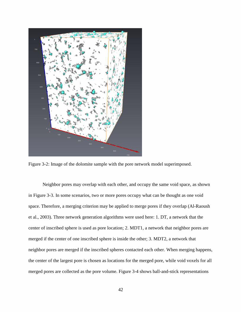
42

Figure 3-2: Image of the dolomite sample with the pore network model superimposed.

Neighbor pores may overlap with each other, and occupy the same void space, as shown

in Figure 3-3. In some scenarios, two or more pores occupy what can be thought as one void

space. Therefore, a merging criterion may be applied to merge pores if they overlap (Al-Raoush

et al., 2003). Three network generation algorithms were used here: 1. DT, a network that the

center of inscribed sphere is used as pore location; 2. MDT1, a network that neighbor pores are

merged if the center of one inscribed sphere is inside the other; 3. MDT2, a network that

neighbor pores are merged if the inscribed spheres contacted each other. When merging happens,

the center of the largest pore is chosen as locations for the merged pore, while void voxels for all

merged pores are collected as the pore volume. Figure 3-4 shows ball-and-stick representations

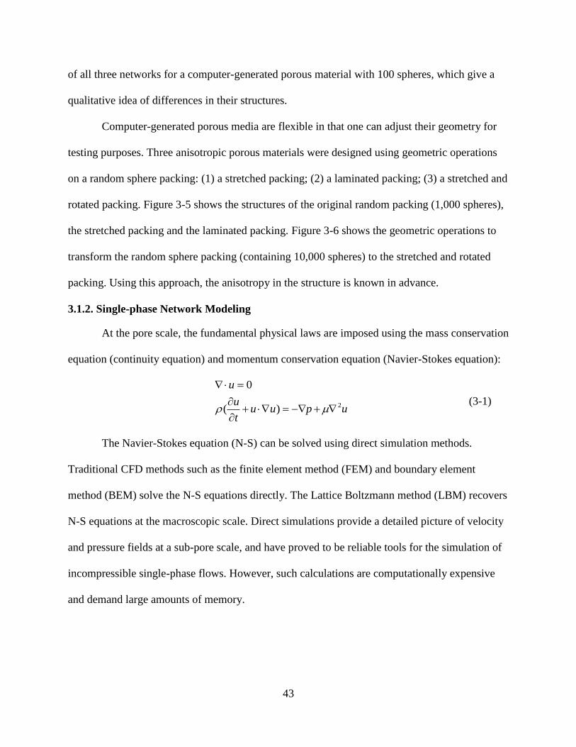
43

of all three networks for a computer-generated porous material with 100 spheres, which give a

qualitative idea of differences in their structures.

Computer-generated porous media are flexible in that one can adjust their geometry for

testing purposes. Three anisotropic porous materials were designed using geometric operations

on a random sphere packing: (1) a stretched packing; (2) a laminated packing; (3) a stretched and

rotated packing. Figure 3-5 shows the structures of the original random packing (1,000 spheres),

the stretched packing and the laminated packing. Figure 3-6 shows the geometric operations to

transform the random sphere packing (containing 10,000 spheres) to the stretched and rotated

packing. Using this approach, the anisotropy in the structure is known in advance.

3.1.2. Single-phase Network Modeling

At the pore scale, the fundamental physical laws are imposed using the mass conservation

equation (continuity equation) and momentum conservation equation (Navier-Stokes equation):

upuut

u

u

2)(

0

(3-1)

The Navier-Stokes equation (N-S) can be solved using direct simulation methods.

Traditional CFD methods such as the finite element method (FEM) and boundary element

method (BEM) solve the N-S equations directly. The Lattice Boltzmann method (LBM) recovers

N-S equations at the macroscopic scale. Direct simulations provide a detailed picture of velocity

and pressure fields at a sub-pore scale, and have proved to be reliable tools for the simulation of

incompressible single-phase flows. However, such calculations are computationally expensive

and demand large amounts of memory.

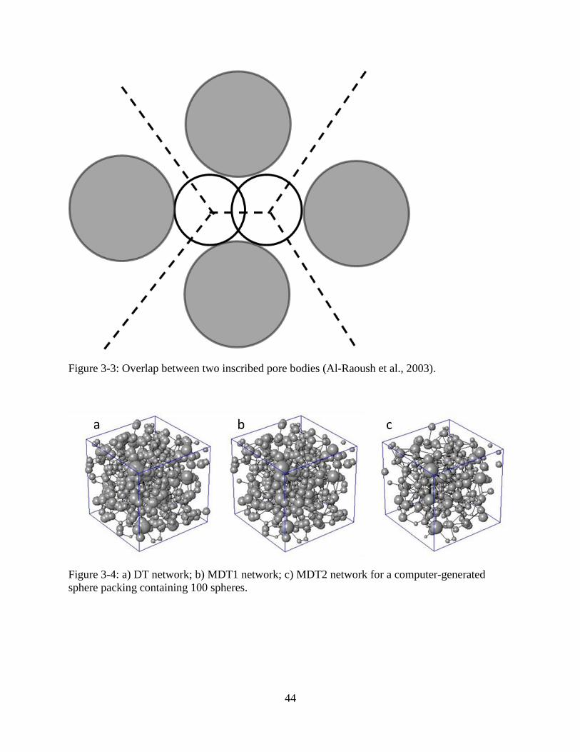
44

Figure 3-3: Overlap between two inscribed pore bodies (Al-Raoush et al., 2003).

Figure 3-4: a) DT network; b) MDT1 network; c) MDT2 network for a computer-generated

sphere packing containing 100 spheres.

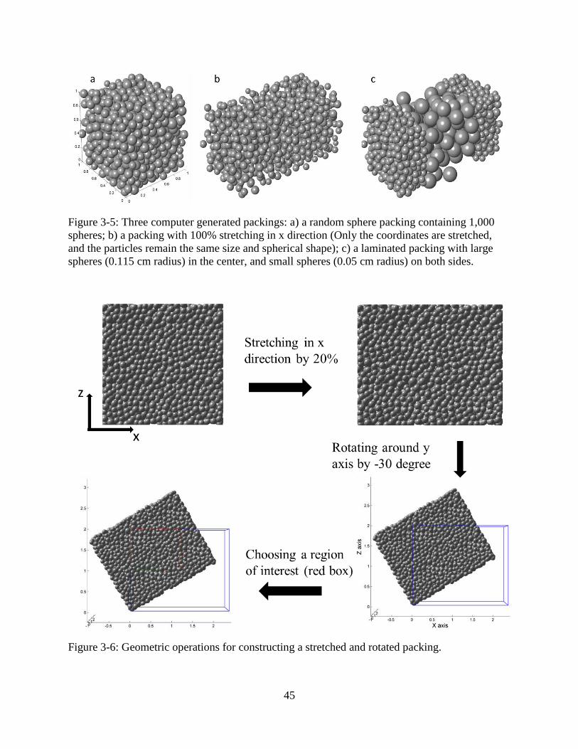
45

Figure 3-5: Three computer generated packings: a) a random sphere packing containing 1,000

spheres; b) a packing with 100% stretching in x direction (Only the coordinates are stretched,

and the particles remain the same size and spherical shape); c) a laminated packing with large

spheres (0.115 cm radius) in the center, and small spheres (0.05 cm radius) on both sides.

Figure 3-6: Geometric operations for constructing a stretched and rotated packing.

46

An alternative approach is to use network simulation. In a pore network model, the pore

space is mapped onto an interconnected set of pores and pore throats. The pores contain the void

space, and the throats control the ability and rate to transmit the fluids. For low-Reynolds-

number flow of a Newtonian fluid, the governing equations for network models are the

following:

)( ji

ij

ij ppg

q

(3-2)

This governing equation is equivalent to the continuity equation at the pore scale. Throat

conductances are estimated using a set of parameters that characterize the physical dimensions of

the local pore space, and can be derived from N-S equations based on simplifications in both

fluid dynamics and pore geometry (Appendix A). To close the network model, boundary

conditions must be specified. Two types of network boundary conditions can be used: constant

injection flow rate or constant applied pressure gradient. For the constant pressure case, the inlet

pores have a constant but nonzero pressure, and pressures in the outlet pores can be set to zero.

For the constant injection rate case, a boundary equation is added, and the inlet pressure pinlet is

an additional unknown from the boundary condition. The linear systems of equations are solved

using library solver for sparse systems.

0)( inletporej

ji

ijpp

g

(3-3)

3.1.3. Permeability Prediction using Network Modeling

Permeability characterizes the fluid transmissibility of a rock sample, which can be

considered an intrinsic parameter of the rock at a given state. Permeability is usually measured

on cylindrical core samples by applying a constant pressure difference or a constant flow rate.

Numerically, permeability can be predicted by solving the fluid flow equations. With the

47

pressure field determined using network modeling, permeability can be calculated using Darcy’s

law:

j

iij

pA

Qk

(3-4)

One could measure the directional permeability by imposing a pressure gradient in the x,

y, or z direction if the pressure gradients are aligned with the principal flow directions. However,

this becomes invalid for anisotropic porous materials if the pressure gradients are different from

the principal flow directions. In real rock samples, permeability is generally anisotropic because

of depositional effects and in-situ stress. It strongly depends on the sample size and the

resolution of the sampling method (Anderson et al., 1994). Anisotropic permeability is usually

measured using large-scale methods such as core measurements. In order to quantify anisotropic

permeability at a finer scale and understand the fundamental physics, three separate simulations

must be run in three independent directions. From linear algebra, the principal values of the

permeability tensor are obtained from the eigenvalues of the permeability tensor (Peters, 2004).

The principal axes of the permeability anisotropy are given by the angles between the

eigenvectors of the permeability tensor and the unit vectors of the coordinate system (Appendix

C). In this Chapter, a novel algorithm is developed to compute the permeability tensor and

principal flow directions using network modeling, which has not previously been done because

of numerical issues such as boundary conditions.

3.1.4. Network Model Validation

Over the years, the most common network validation method is permeability comparison.

While permeability agreement is essential in practice, it is not sufficient from a fundamental

perspective. Permeability is an average macroscopic parameter that can be correctly predicted for

synthetic sphere packings using empirical models such as Kozeny-Carman equation. However,

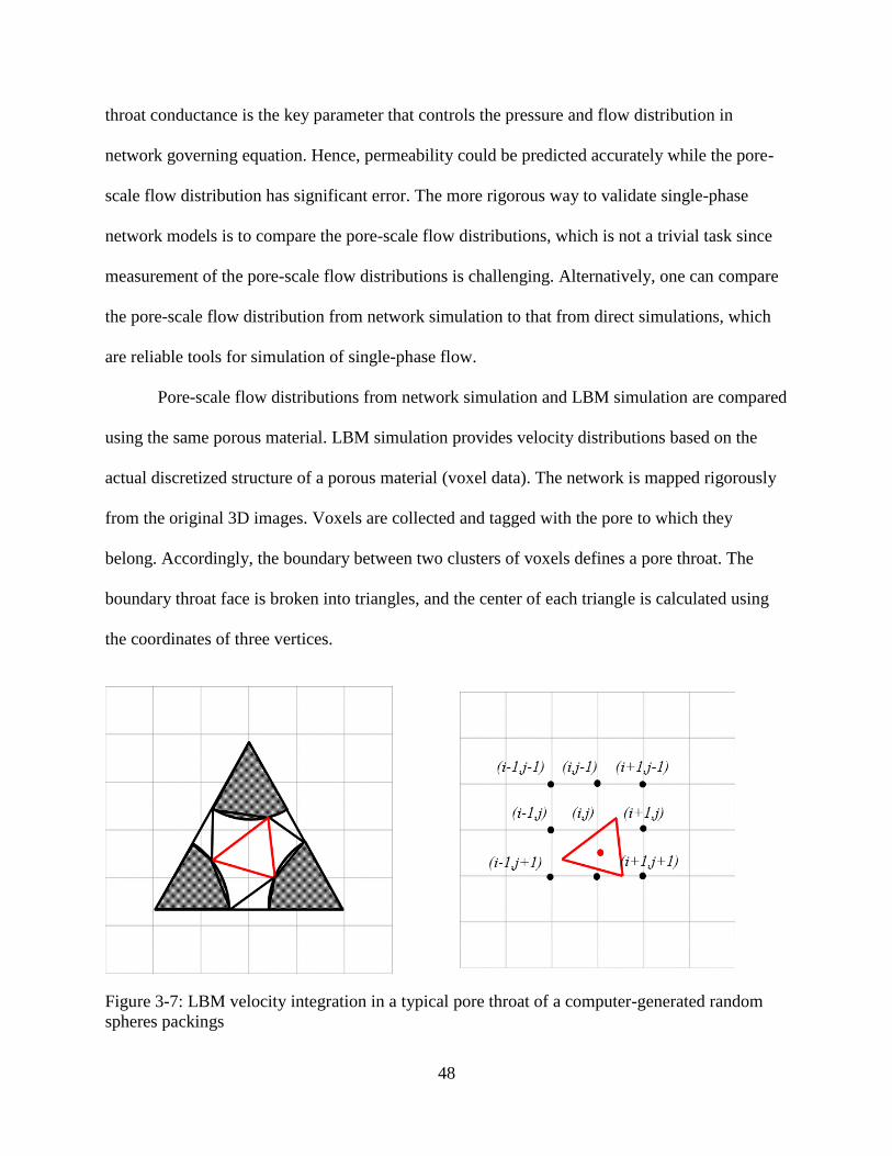
48

throat conductance is the key parameter that controls the pressure and flow distribution in

network governing equation. Hence, permeability could be predicted accurately while the pore-

scale flow distribution has significant error. The more rigorous way to validate single-phase

network models is to compare the pore-scale flow distributions, which is not a trivial task since

measurement of the pore-scale flow distributions is challenging. Alternatively, one can compare

the pore-scale flow distribution from network simulation to that from direct simulations, which

are reliable tools for simulation of single-phase flow.

Pore-scale flow distributions from network simulation and LBM simulation are compared

using the same porous material. LBM simulation provides velocity distributions based on the

actual discretized structure of a porous material (voxel data). The network is mapped rigorously

from the original 3D images. Voxels are collected and tagged with the pore to which they

belong. Accordingly, the boundary between two clusters of voxels defines a pore throat. The

boundary throat face is broken into triangles, and the center of each triangle is calculated using

the coordinates of three vertices.

Figure 3-7: LBM velocity integration in a typical pore throat of a computer-generated random

spheres packings

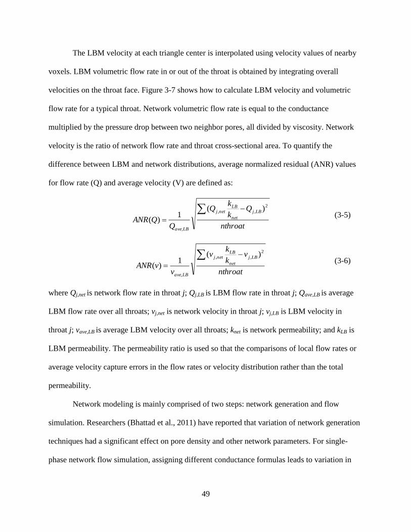
49

The LBM velocity at each triangle center is interpolated using velocity values of nearby

voxels. LBM volumetric flow rate in or out of the throat is obtained by integrating overall

velocities on the throat face. Figure 3-7 shows how to calculate LBM velocity and volumetric

flow rate for a typical throat. Network volumetric flow rate is equal to the conductance

multiplied by the pressure drop between two neighbor pores, all divided by viscosity. Network

velocity is the ratio of network flow rate and throat cross-sectional area. To quantify the

difference between LBM and network distributions, average normalized residual (ANR) values

for flow rate (Q) and average velocity (V) are defined as:

nthroat

Qk

kQ

QQANR

LBj

net

LBnetj

LBave

2

,,

,

)(1

)( (3-5)

nthroat

vk

kv

vvANR

LBj

net

LBnetj

LBave

2

,,

,

)(1

)( (3-6)

where Qj,net is network flow rate in throat j; Qj,LB is LBM flow rate in throat j; Qave,LB is average

LBM flow rate over all throats; vj,net is network velocity in throat j; vj,LB is LBM velocity in

throat j; vave,LB is average LBM velocity over all throats; knet is network permeability; and kLB is

LBM permeability. The permeability ratio is used so that the comparisons of local flow rates or

average velocity capture errors in the flow rates or velocity distribution rather than the total

permeability.

Network modeling is mainly comprised of two steps: network generation and flow

simulation. Researchers (Bhattad et al., 2011) have reported that variation of network generation

techniques had a significant effect on pore density and other network parameters. For single-

phase network flow simulation, assigning different conductance formulas leads to variation in

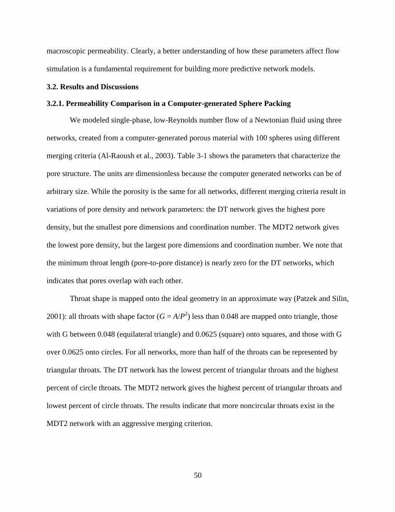
50

macroscopic permeability. Clearly, a better understanding of how these parameters affect flow

simulation is a fundamental requirement for building more predictive network models.

3.2. Results and Discussions

3.2.1. Permeability Comparison in a Computer-generated Sphere Packing

We modeled single-phase, low-Reynolds number flow of a Newtonian fluid using three

networks, created from a computer-generated porous material with 100 spheres using different

merging criteria (Al-Raoush et al., 2003). Table 3-1 shows the parameters that characterize the

pore structure. The units are dimensionless because the computer generated networks can be of

arbitrary size. While the porosity is the same for all networks, different merging criteria result in

variations of pore density and network parameters: the DT network gives the highest pore

density, but the smallest pore dimensions and coordination number. The MDT2 network gives

the lowest pore density, but the largest pore dimensions and coordination number. We note that

the minimum throat length (pore-to-pore distance) is nearly zero for the DT networks, which

indicates that pores overlap with each other.

Throat shape is mapped onto the ideal geometry in an approximate way (Patzek and Silin,

2001): all throats with shape factor (G = A/P2) less than 0.048 are mapped onto triangle, those

with G between 0.048 (equilateral triangle) and 0.0625 (square) onto squares, and those with G

over 0.0625 onto circles. For all networks, more than half of the throats can be represented by

triangular throats. The DT network has the lowest percent of triangular throats and the highest

percent of circle throats. The MDT2 network gives the highest percent of triangular throats and

lowest percent of circle throats. The results indicate that more noncircular throats exist in the

MDT2 network with an aggressive merging criterion.

51

Table 3-1: Networks parameters using different merging criteria

Variables DT MDT1 MDT2

Pore Number of pores 619 412 259

Porosity (%) 37.98 37.99 37.99

Pore volume (min/ave/max) 0.011/0.052/0.143 0.011/0.078/0.603 0.027/0.124/0.974

Inscribed radius (min/ave/max) 0.058/0.195/0.374 0.058/0.179/0.374 0.058/0.174/0.374

Coordination number (min/ave/max) 4 3/4.59/12 1/5.43/16

Throat Effective radius (min/ave/max) 0.113/0.189/0.398 0.113/0.178/0.424 0.113/0.172/0.522

Surface area (min/ave/max) 0.006/0.254/0.531 0.094/0.334/1.042 0.104/0.454/2.337

Inscribed radius (min/ave/max) 0.077/0.151/0.353 0.065/0.132/0.353 0.030/0.117/0.291

Length (min/ave/max) 0.000/0.414/1.113 0.175/0.532/1.230 0.282/0.695/1.630

Throat shape (% of triangular/rectangular/circle) 75.8/14.5/9.6 86.8/11.0/2.2 95.2/4.1/0.7

Aspect ratio (min/ave/max) 0.240/0.798/4.204 0.204/0.737/3.575 0.141/0.658/3.575

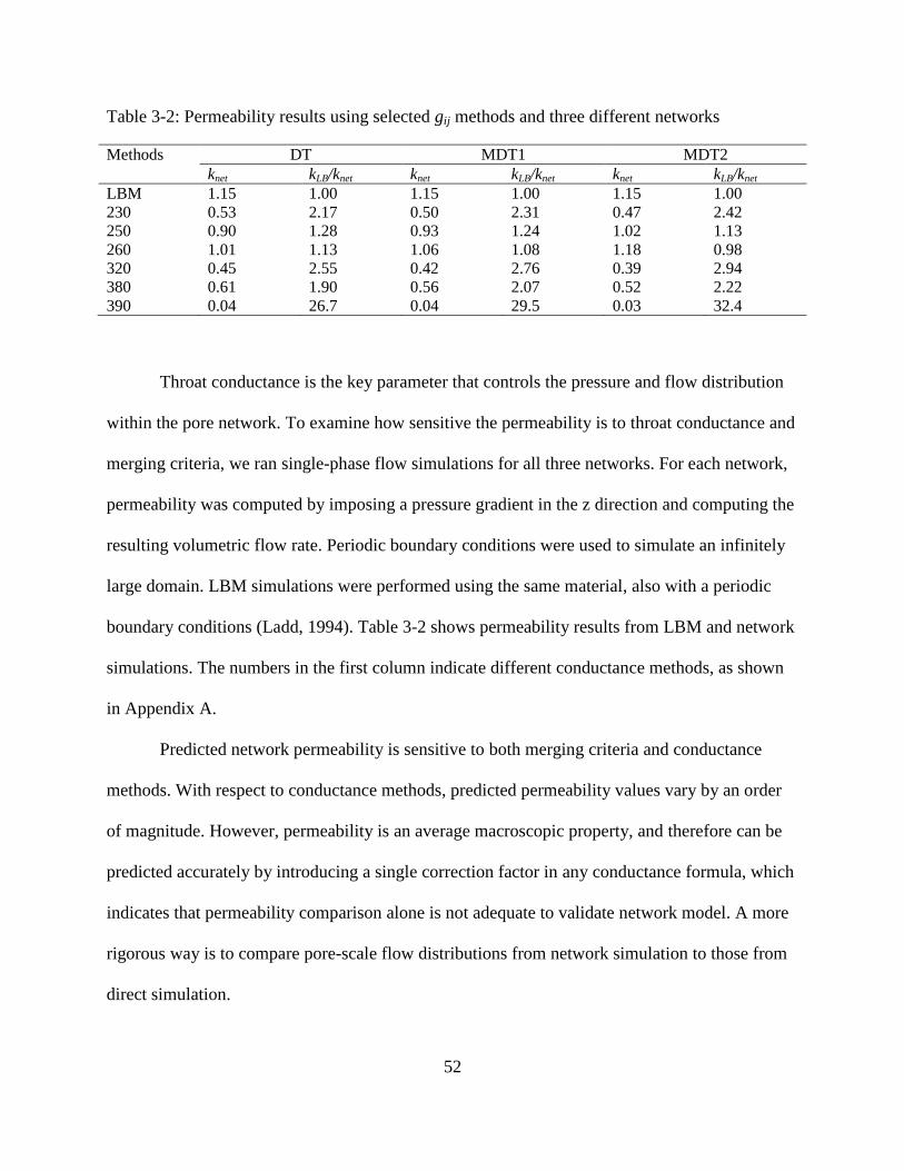
52

Table 3-2: Permeability results using selected gij methods and three different networks

Methods DT MDT1 MDT2

knet kLB/knet knet kLB/knet knet kLB/knet

LBM 1.15 1.00 1.15 1.00 1.15 1.00

230 0.53 2.17 0.50 2.31 0.47 2.42

250 0.90 1.28 0.93 1.24 1.02 1.13

260 1.01 1.13 1.06 1.08 1.18 0.98

320 0.45 2.55 0.42 2.76 0.39 2.94

380 0.61 1.90 0.56 2.07 0.52 2.22

390 0.04 26.7 0.04 29.5 0.03 32.4

Throat conductance is the key parameter that controls the pressure and flow distribution

within the pore network. To examine how sensitive the permeability is to throat conductance and

merging criteria, we ran single-phase flow simulations for all three networks. For each network,

permeability was computed by imposing a pressure gradient in the z direction and computing the

resulting volumetric flow rate. Periodic boundary conditions were used to simulate an infinitely

large domain. LBM simulations were performed using the same material, also with a periodic

boundary conditions (Ladd, 1994). Table 3-2 shows permeability results from LBM and network

simulations. The numbers in the first column indicate different conductance methods, as shown

in Appendix A.

Predicted network permeability is sensitive to both merging criteria and conductance

methods. With respect to conductance methods, predicted permeability values vary by an order

of magnitude. However, permeability is an average macroscopic property, and therefore can be

predicted accurately by introducing a single correction factor in any conductance formula, which

indicates that permeability comparison alone is not adequate to validate network model. A more

rigorous way is to compare pore-scale flow distributions from network simulation to those from

direct simulation.

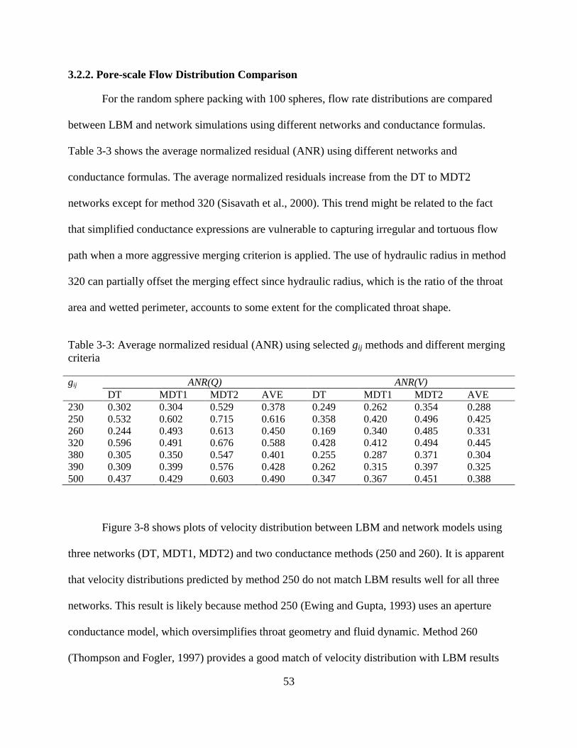
53

3.2.2. Pore-scale Flow Distribution Comparison

For the random sphere packing with 100 spheres, flow rate distributions are compared

between LBM and network simulations using different networks and conductance formulas.

Table 3-3 shows the average normalized residual (ANR) using different networks and

conductance formulas. The average normalized residuals increase from the DT to MDT2

networks except for method 320 (Sisavath et al., 2000). This trend might be related to the fact

that simplified conductance expressions are vulnerable to capturing irregular and tortuous flow

path when a more aggressive merging criterion is applied. The use of hydraulic radius in method

320 can partially offset the merging effect since hydraulic radius, which is the ratio of the throat

area and wetted perimeter, accounts to some extent for the complicated throat shape.

Table 3-3: Average normalized residual (ANR) using selected gij methods and different merging

criteria

gij ANR(Q) ANR(V)

DT MDT1 MDT2 AVE DT MDT1 MDT2 AVE

230 0.302 0.304 0.529 0.378 0.249 0.262 0.354 0.288

250 0.532 0.602 0.715 0.616 0.358 0.420 0.496 0.425

260 0.244 0.493 0.613 0.450 0.169 0.340 0.485 0.331

320 0.596 0.491 0.676 0.588 0.428 0.412 0.494 0.445

380 0.305 0.350 0.547 0.401 0.255 0.287 0.371 0.304

390 0.309 0.399 0.576 0.428 0.262 0.315 0.397 0.325

500 0.437 0.429 0.603 0.490 0.347 0.367 0.451 0.388

Figure 3-8 shows plots of velocity distribution between LBM and network models using

three networks (DT, MDT1, MDT2) and two conductance methods (250 and 260). It is apparent

that velocity distributions predicted by method 250 do not match LBM results well for all three

networks. This result is likely because method 250 (Ewing and Gupta, 1993) uses an aperture

conductance model, which oversimplifies throat geometry and fluid dynamic. Method 260

(Thompson and Fogler, 1997) provides a good match of velocity distribution with LBM results

54

for the DT network. The disparity between network and LBM results grows from the DT to

MDT2 network. This observation is consistent with the average normalized residual results,

which show an increase in ANR values when a more aggressive merging criterion is applied.

Among all tested conductance methods, method 260 provides the best match of velocity

distribution with LBM results for the DT network. This is not surprising since method 260 uses a

BEM approach to estimate 2D throat conductance, and also accounts for the converging

diverging feature using a Venturi approximation.

Method 260 provides a good match of velocity distribution with LBM results for the DT

network. However, this conductance computation is time consuming because the numerical

BEM computations are performed locally to calculate conductance for the true cross-sectional

shape in each throat. An exponential conductance expression is derived using the least-squares

fitting of BEM conductance (Sholokhova et al., 2009). Figure 3-9 shows BEM conductance

distribution versus shape factor and its corresponding fitted function for the DT network.

Average normalized residuals (ANR) are 0.205 for flow rate, which are slightly reduced from

ANR of the original method 260 (ANR = 0.244). Additionally, BEM conductances have been

fitted versus other geometric parameters such as throat radius, length, and cross-sectional area.

The results show that shape factor is the best choice out of the parameters tested.

3.2.3. Permeability for Anisotropic Porous Media

We ran simulations for three computer-generated porous materials: (1) a random sphere

packing containing 1,000 spheres; (2) a stretched packing; (3) a laminated packing. Periodic

conditions were used for all simulations, in which the fluid leaving one side of the domain

reentered at the opposite plane. For validation, network results were compared with values from

finite element (FEM) simulations for stokes flow.

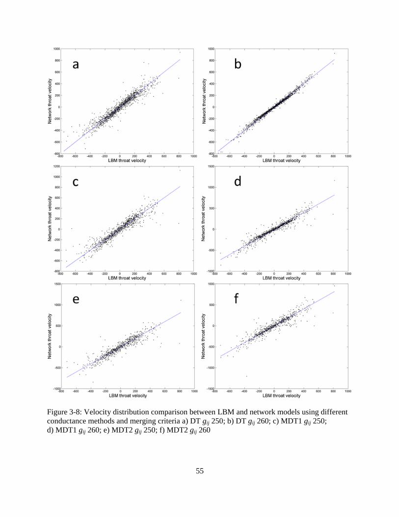
55

Figure 3-8: Velocity distribution comparison between LBM and network models using different

conductance methods and merging criteria a) DT gij 250; b) DT gij 260; c) MDT1 gij 250;

d) MDT1 gij 260; e) MDT2 gij 250; f) MDT2 gij 260

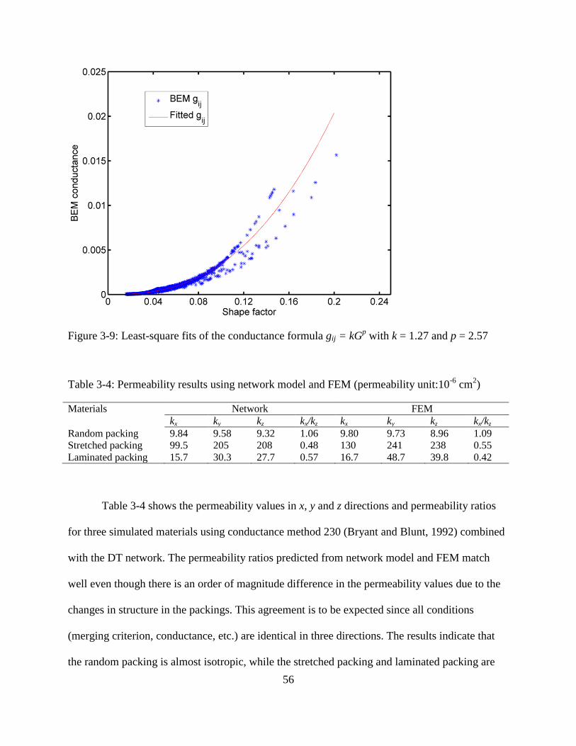
56

Figure 3-9: Least-square fits of the conductance formula gij = kGp with k = 1.27 and p = 2.57

Table 3-4: Permeability results using network model and FEM (permeability unit:10-6

cm2)

Materials Network FEM kx ky kz kx/kz kx ky kz kx/kz Random packing 9.84 9.58 9.32 1.06 9.80 9.73 8.96 1.09 Stretched packing 99.5 205 208 0.48 130 241 238 0.55 Laminated packing 15.7 30.3 27.7 0.57 16.7 48.7 39.8 0.42

Table 3-4 shows the permeability values in x, y and z directions and permeability ratios

for three simulated materials using conductance method 230 (Bryant and Blunt, 1992) combined

with the DT network. The permeability ratios predicted from network model and FEM match

well even though there is an order of magnitude difference in the permeability values due to the

changes in structure in the packings. This agreement is to be expected since all conditions

(merging criterion, conductance, etc.) are identical in three directions. The results indicate that

the random packing is almost isotropic, while the stretched packing and laminated packing are

57

highly anisotropic, with a higher permeability values in the y and z directions. For the stretched

packing, permeability values in the y and z directions increase since flow channels expand

radially because of the stretching. For the laminated packing, higher permeability values in the y

and z directions result from the high permeability layer in the center of the packing.

Table 3-5: Permeability results using different merging criteria and conductance methods for the

stretched porous medium with a porosity equal to 68.97% (permeability unit:10-6

cm2)

Method kx ky kz kx/kz

FEM 130 241 238 0.55

MDT1 210 20.0 38.6 39.7 0.50

230 99.5 205 208 0.48

250 84.0 129 133 0.63

380 46.1 95.4 96.8 0.48

MDT2 210 3.76 3.55 2.46 1.53

230 28.4 27.0 18.5 1.53

250 22.4 21.3 15.9 1.41

380 12.3 11.7 8.02 1.53

We examined how sensitive the anisotropic permeability is to network structure and

conductance methods for the stretched network with porosity equal to 68.97%, as shown in Table

3-5. The permeability ratio is relatively insensitive to the conductance formulas although there is

significant difference in the permeability values for the two tested networks. The exception is

method 250 (Ewing and Gupta, 1993), which deviates from the values of other conductance

methods significantly, because this method oversimplifies the pore throat as an aperture. Another

important observation is that varying merging criteria change both permeability values and

permeability ratios. Predicted permeability ratios using the MDT1 network match the FEM

permeability ratio, while permeability ratios using the MDT2 network deviate from FEM

permeability ratio significantly. Additional tests show that the permeability ratio is relatively

insensitive to merging criteria for the random and laminated packings with porosity equal to

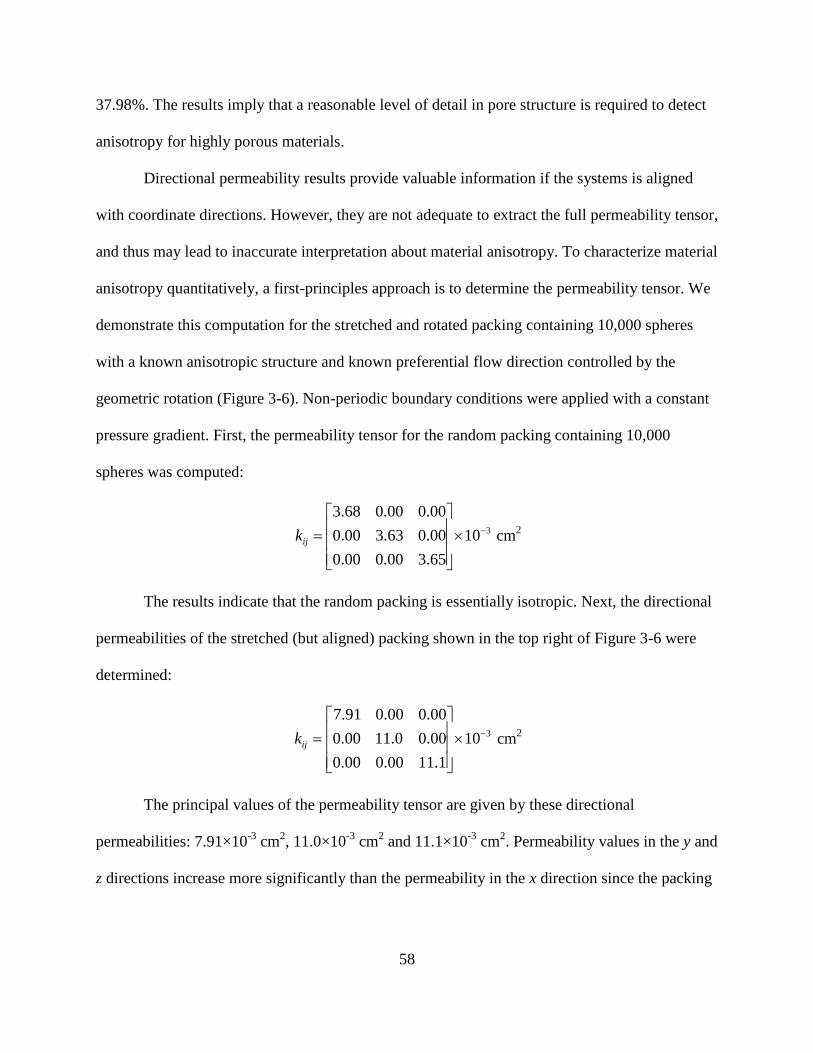
58

37.98%. The results imply that a reasonable level of detail in pore structure is required to detect

anisotropy for highly porous materials.

Directional permeability results provide valuable information if the systems is aligned

with coordinate directions. However, they are not adequate to extract the full permeability tensor,

and thus may lead to inaccurate interpretation about material anisotropy. To characterize material

anisotropy quantitatively, a first-principles approach is to determine the permeability tensor. We

demonstrate this computation for the stretched and rotated packing containing 10,000 spheres

with a known anisotropic structure and known preferential flow direction controlled by the

geometric rotation (Figure 3-6). Non-periodic boundary conditions were applied with a constant

pressure gradient. First, the permeability tensor for the random packing containing 10,000

spheres was computed:

310

65.300.000.0

00.063.300.0

00.000.068.3

ijk cm2

The results indicate that the random packing is essentially isotropic. Next, the directional

permeabilities of the stretched (but aligned) packing shown in the top right of Figure 3-6 were

determined:

310

1.1100.000.0

00.00.1100.0

00.000.091.7

ijk cm2

The principal values of the permeability tensor are given by these directional

permeabilities: 7.91×10-3

cm2, 11.0×10

-3 cm

2 and 11.1×10

-3 cm

2. Permeability values in the y and

z directions increase more significantly than the permeability in the x direction since the packing

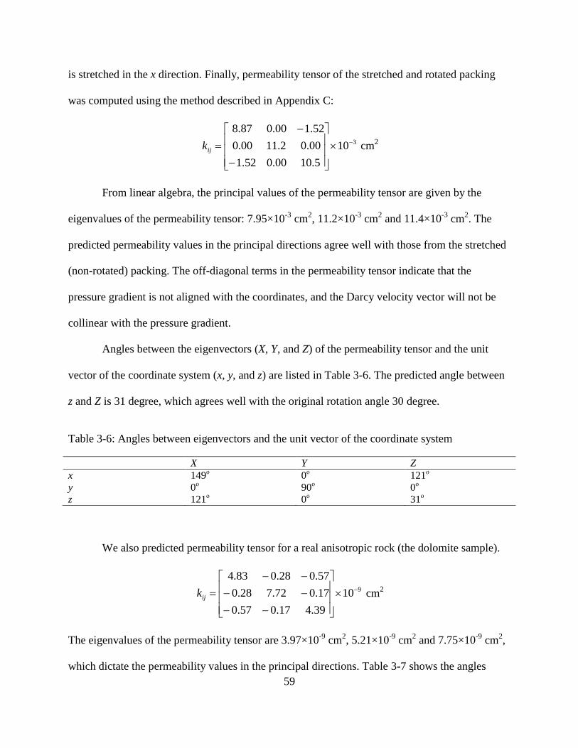
59

is stretched in the x direction. Finally, permeability tensor of the stretched and rotated packing

was computed using the method described in Appendix C:

310

5.1000.052.1

00.02.1100.0

52.100.087.8

ijk cm2

From linear algebra, the principal values of the permeability tensor are given by the

eigenvalues of the permeability tensor: 7.95×10-3

cm2, 11.2×10

-3 cm

2 and 11.4×10

-3 cm

2. The

predicted permeability values in the principal directions agree well with those from the stretched

(non-rotated) packing. The off-diagonal terms in the permeability tensor indicate that the

pressure gradient is not aligned with the coordinates, and the Darcy velocity vector will not be

collinear with the pressure gradient.

Angles between the eigenvectors (X, Y, and Z) of the permeability tensor and the unit

vector of the coordinate system (x, y, and z) are listed in Table 3-6. The predicted angle between

z and Z is 31 degree, which agrees well with the original rotation angle 30 degree.

Table 3-6: Angles between eigenvectors and the unit vector of the coordinate system

X Y Z

x 149ο 0

ο 121

ο

y 0ο 90

ο 0

ο

z 121ο 0

ο 31

ο

We also predicted permeability tensor for a real anisotropic rock (the dolomite sample).

910

39.417.057.0

17.072.728.0

57.028.083.4

ijk cm2

The eigenvalues of the permeability tensor are 3.97×10-9

cm2, 5.21×10

-9 cm

2 and 7.75×10

-9 cm

2,

which dictate the permeability values in the principal directions. Table 3-7 shows the angles

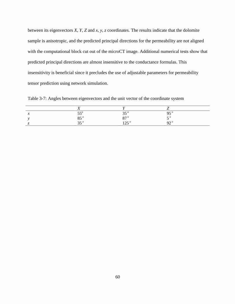
60

between its eigenvectors X, Y, Z and x, y, z coordinates. The results indicate that the dolomite

sample is anisotropic, and the predicted principal directions for the permeability are not aligned

with the computational block cut out of the microCT image. Additional numerical tests show that

predicted principal directions are almost insensitive to the conductance formulas. This

insensitivity is beneficial since it precludes the use of adjustable parameters for permeability

tensor prediction using network simulation.

Table 3-7: Angles between eigenvectors and the unit vector of the coordinate system

X Y Z

x 55ο 35

ο 95

ο

y 85 ο 87

ο 5

ο

z 35 ο 125

ο 92

ο

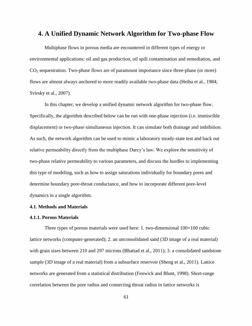
61

4. A Unified Dynamic Network Algorithm for Two-phase Flow

Multiphase flows in porous media are encountered in different types of energy or

environmental applications: oil and gas production, oil spill contamination and remediation, and

CO2 sequestration. Two-phase flows are of paramount importance since three-phase (or more)

flows are almost always anchored to more readily available two-phase data (Heiba et al., 1984;

Svirsky et al., 2007).

In this chapter, we develop a unified dynamic network algorithm for two-phase flow.

Specifically, the algorithm described below can be run with one-phase injection (i.e. immiscible

displacement) or two-phase simultaneous injection. It can simulate both drainage and imbibition.

As such, the network algorithm can be used to mimic a laboratory steady-state test and back out

relative permeability directly from the multiphase Darcy’s law. We explore the sensitivity of

two-phase relative permeability to various parameters, and discuss the hurdles to implementing

this type of modeling, such as how to assign saturations individually for boundary pores and

determine boundary pore-throat conductance, and how to incorporate different pore-level

dynamics in a single algorithm.

4.1. Methods and Materials


Three types of porous materials were used here: 1. two-dimensional 100×100 cubic

lattice networks (computer-generated); 2. an unconsolidated sand (3D image of a real material)

with grain sizes between 210 and 297 microns (Bhattad et al., 2011); 3. a consolidated sandstone

sample (3D image of a real material) from a subsurface reservoir (Sheng et al., 2011). Lattice

networks are generated from a statistical distribution (Fenwick and Blunt, 1998). Short-range

correlation between the pore radius and connecting throat radius in lattice networks is

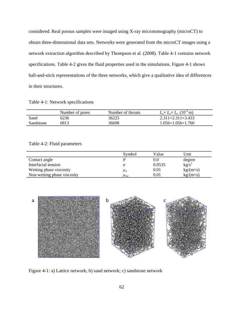
62

considered. Real porous samples were imaged using X-ray microtomography (microCT) to

obtain three-dimensional data sets. Networks were generated from the microCT images using a

network extraction algorithm described by Thompson et al. (2008). Table 4-1 contains network

specifications. Table 4-2 gives the fluid properties used in the simulations. Figure 4-1 shows

ball-and-stick representations of the three networks, which give a qualitative idea of differences

in their structures.

Table 4-1: Network specifications

Number of pores Number of throats Lx× Ly× Lz (10

-3 m)

Sand 6236 36225 2.311×2.311×3.433 Sandstone 6813 36698 1.056×1.056×1.760

Table 4-2: Fluid parameters

Symbol Value Unit

Contact angle θ 0.0 degree Interfacial tension σ 0.0535 kg/s

2 Wetting phase viscosity μw 0.01 kg/(m×s) Non-wetting phase viscosity μnw 0.01 kg/(m×s)

Figure 4-1: a) Lattice network; b) sand network; c) sandstone network

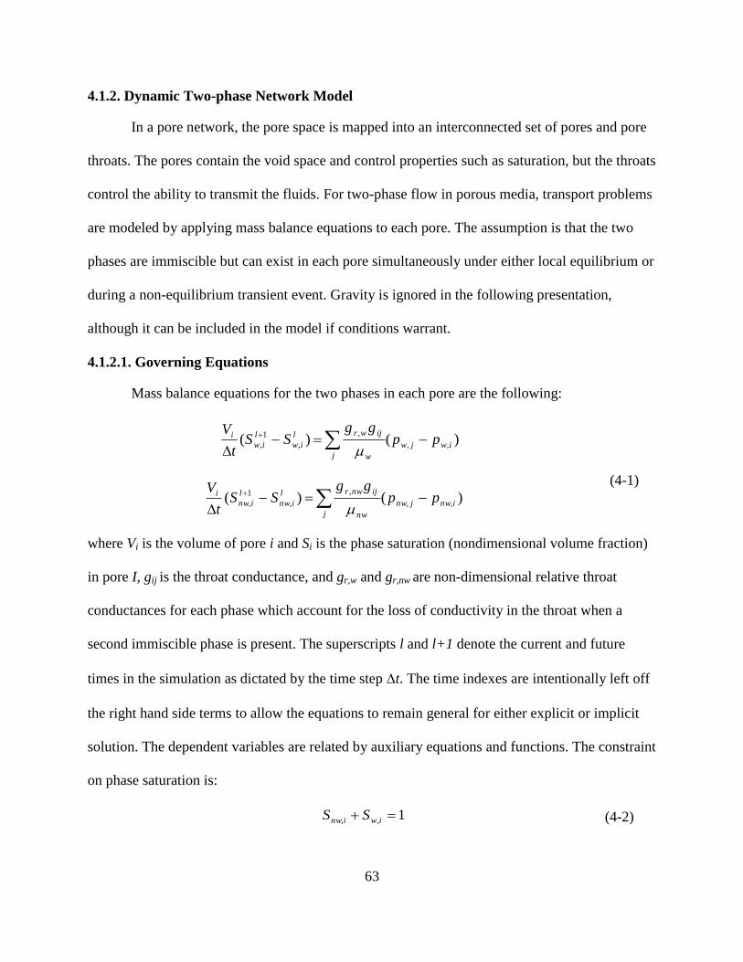
63

4.1.2. Dynamic Two-phase Network Model

In a pore network, the pore space is mapped into an interconnected set of pores and pore

throats. The pores contain the void space and control properties such as saturation, but the throats

control the ability to transmit the fluids. For two-phase flow in porous media, transport problems

are modeled by applying mass balance equations to each pore. The assumption is that the two

phases are immiscible but can exist in each pore simultaneously under either local equilibrium or

during a non-equilibrium transient event. Gravity is ignored in the following presentation,

although it can be included in the model if conditions warrant.

4.1.2.1. Governing Equations

Mass balance equations for the two phases in each pore are the following:

)()( ,,

,

,

1

, iwjw

j w

ijwrl

iw

l

iw

i ppgg

SSt

V

(4-1)

)()( ,,

,

,

1

, inwjnw

j nw

ijnwrl

inw

l

inw

i ppgg

SSt

V

where Vi is the volume of pore i and Si is the phase saturation (nondimensional volume fraction)

in pore I, gij is the throat conductance, and gr,w and gr,nw are non-dimensional relative throat

conductances for each phase which account for the loss of conductivity in the throat when a

second immiscible phase is present. The superscripts l and l+1 denote the current and future

times in the simulation as dictated by the time step t. The time indexes are intentionally left off

the right hand side terms to allow the equations to remain general for either explicit or implicit

solution. The dependent variables are related by auxiliary equations and functions. The constraint

on phase saturation is:

1,, iwinw SS (4-2)

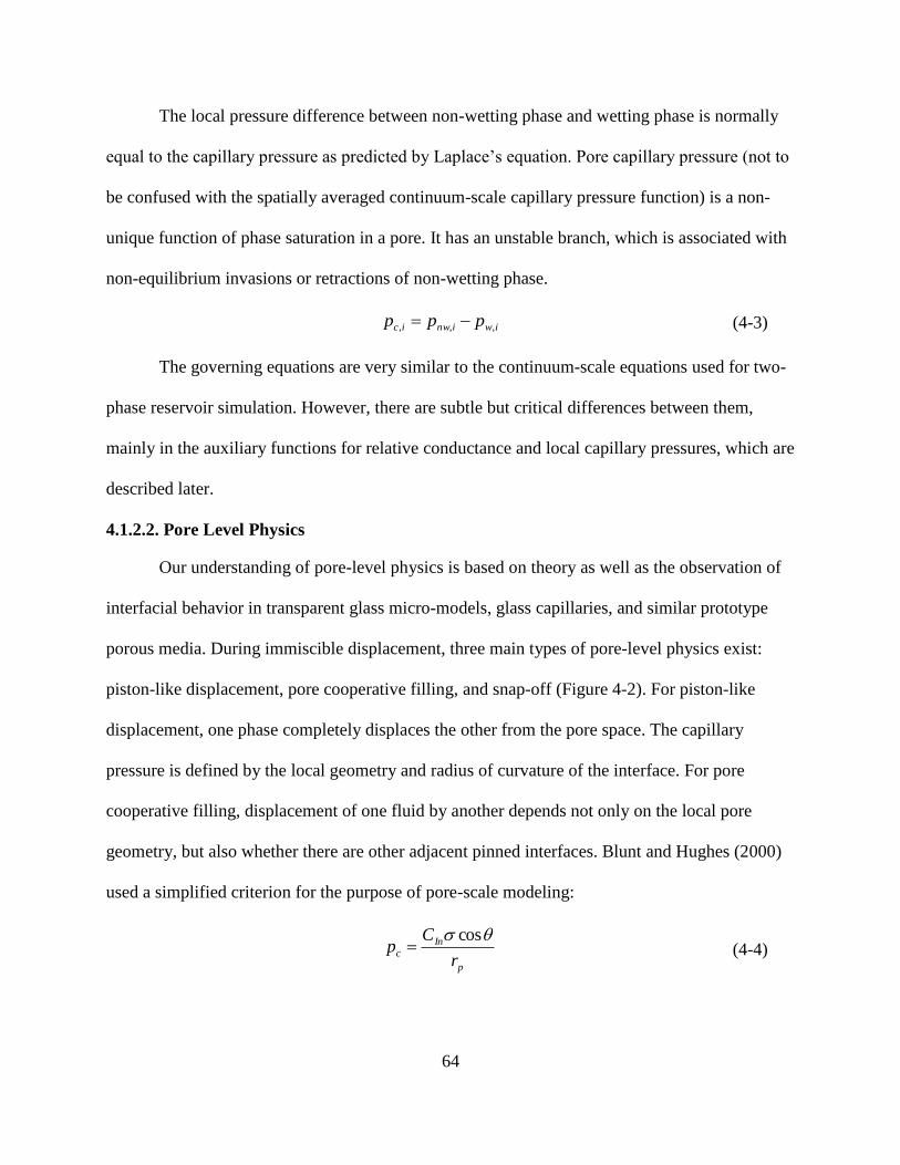
64

The local pressure difference between non-wetting phase and wetting phase is normally

equal to the capillary pressure as predicted by Laplace’s equation. Pore capillary pressure (not to

be confused with the spatially averaged continuum-scale capillary pressure function) is a non-

unique function of phase saturation in a pore. It has an unstable branch, which is associated with

non-equilibrium invasions or retractions of non-wetting phase.

iwinwic ppp ,,, (4-3)

The governing equations are very similar to the continuum-scale equations used for two-

phase reservoir simulation. However, there are subtle but critical differences between them,

mainly in the auxiliary functions for relative conductance and local capillary pressures, which are

described later.

4.1.2.2. Pore Level Physics

Our understanding of pore-level physics is based on theory as well as the observation of

interfacial behavior in transparent glass micro-models, glass capillaries, and similar prototype

porous media. During immiscible displacement, three main types of pore-level physics exist:

piston-like displacement, pore cooperative filling, and snap-off (Figure 4-2). For piston-like

displacement, one phase completely displaces the other from the pore space. The capillary

pressure is defined by the local geometry and radius of curvature of the interface. For pore

cooperative filling, displacement of one fluid by another depends not only on the local pore

geometry, but also whether there are other adjacent pinned interfaces. Blunt and Hughes (2000)

used a simplified criterion for the purpose of pore-scale modeling:

p

Inc

r

Cp

cos (4-4)

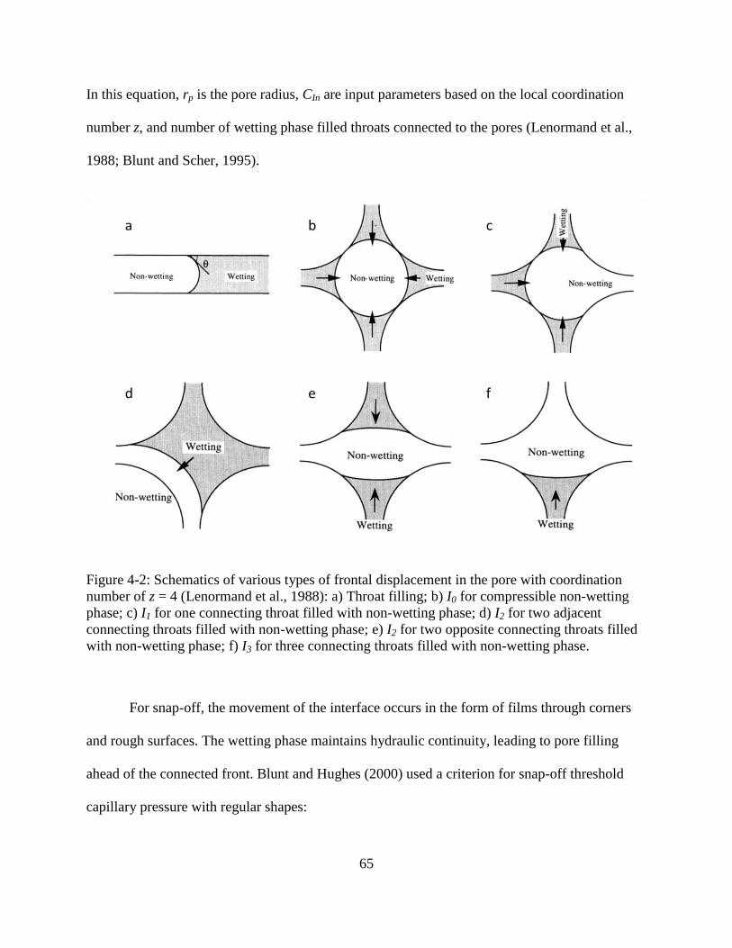
65

In this equation, rp is the pore radius, CIn are input parameters based on the local coordination

number z, and number of wetting phase filled throats connected to the pores (Lenormand et al.,

1988; Blunt and Scher, 1995).

Figure 4-2: Schematics of various types of frontal displacement in the pore with coordination

number of z = 4 (Lenormand et al., 1988): a) Throat filling; b) I0 for compressible non-wetting

phase; c) I1 for one connecting throat filled with non-wetting phase; d) I2 for two adjacent

connecting throats filled with non-wetting phase; e) I2 for two opposite connecting throats filled

with non-wetting phase; f) I3 for three connecting throats filled with non-wetting phase.

For snap-off, the movement of the interface occurs in the form of films through corners

and rough surfaces. The wetting phase maintains hydraulic continuity, leading to pore filling

ahead of the connected front. Blunt and Hughes (2000) used a criterion for snap-off threshold

capillary pressure with regular shapes:

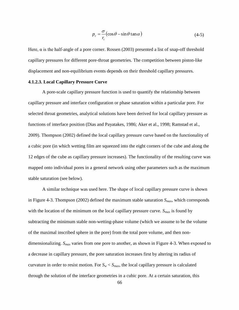
66

tansincos t

cr

p (4-5)

Here, α is the half-angle of a pore corner. Rossen (2003) presented a list of snap-off threshold

capillary pressures for different pore-throat geometries. The competition between piston-like

displacement and non-equilibrium events depends on their threshold capillary pressures.

4.1.2.3. Local Capillary Pressure Curve

A pore-scale capillary pressure function is used to quantify the relationship between

capillary pressure and interface configuration or phase saturation within a particular pore. For

selected throat geometries, analytical solutions have been derived for local capillary pressure as

functions of interface position (Dias and Payatakes, 1986; Aker et al., 1998; Ramstad et al.,

2009). Thompson (2002) defined the local capillary pressure curve based on the functionality of

a cubic pore (in which wetting film are squeezed into the eight corners of the cube and along the

12 edges of the cube as capillary pressure increases). The functionality of the resulting curve was

mapped onto individual pores in a general network using other parameters such as the maximum

stable saturation (see below).

A similar technique was used here. The shape of local capillary pressure curve is shown

in Figure 4-3. Thompson (2002) defined the maximum stable saturation Smax, which corresponds

with the location of the minimum on the local capillary pressure curve. Smax is found by

subtracting the minimum stable non-wetting-phase volume (which we assume to be the volume

of the maximal inscribed sphere in the pore) from the total pore volume, and then non-

dimensionalizing. Smax varies from one pore to another, as shown in Figure 4-3. When exposed to

a decrease in capillary pressure, the pore saturation increases first by altering its radius of

curvature in order to resist motion. For Sw < Smax, the local capillary pressure is calculated

through the solution of the interface geometries in a cubic pore. At a certain saturation, this

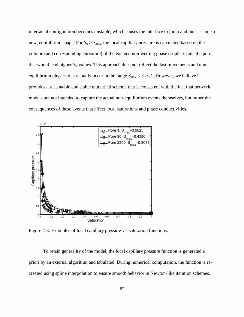
67

interfacial configuration becomes unstable, which causes the interface to jump and thus assume a

new, equilibrium shape. For Sw > Smax, the local capillary pressure is calculated based on the

volume (and corresponding curvature) of the isolated non-wetting phase droplet inside the pore

that would lead higher Sw values. This approach does not reflect the fast movements and non-

equilibrium physics that actually occur in the range Smax < Sw < 1. However, we believe it

provides a reasonable and stable numerical scheme that is consistent with the fact that network

models are not intended to capture the actual non-equilibrium events themselves, but rather the

consequences of these events that affect local saturations and phase conductivities.

Figure 4-3: Examples of local capillary pressure vs. saturation functions.

To retain generality of the model, the local capillary pressure function is generated a

priori by an external algorithm and tabulated. During numerical computation, the function is re-

created using spline interpolation to ensure smooth behavior in Newton-like iteration schemes.

68

The advantages of this approach are computational speed and generality (the latter point being

that the algorithm operates independently of where the Pc(Sw) information originated, thus

allowing more rigorous pore capillary pressure functionalities to be substituted as they are

developed). The disadvantage of an a-priori computation is that it assumes capillary pressure

depends on saturation only. This assumption restricts, for instance, the ability to account for the

variety of invasion patterns and entry pressures caused by cooperative filling. This limitation

could be relaxed if one creates a multivariable tabulation for the local capillary pressure function.

4.1.2.4. Absolute Conductance and Relative Conductance

Absolute conductance gij is estimated using a set of parameters that characterize the

physical dimensions of the pore space. One of the simplest methods maps the network structure

onto a network of capillary tubes, and the Hagen-Poiseuille equation is then applied to calculate

the throat conductance. For the non-circular cross sections found in sphere packings, Bryant et

al. (1993) substituted the effective radius in the Hagen-Poiseuille equation, which is defined as

the arithmetic mean of the inscribed and equivalent-area radii:

t

eff

ijl

Ag

8

2

(4-6)

where the term Aeff is the throat cross-sectional area (Aeff = πr2

eff) and lt is the throat length. A

similar technique can be used for image-based modeling, except local pore geometric

information can be mapped directly from high resolution three-dimensional data such as micro-

tomography images. Thompson and Fogler (1997) computed the throat conductance by

performing numerical simulation of laminar flow through the cross-sectional shape of each pore-

throat, and then applied a correction to account for converging-diverging geometry. Numerous

other conductance formulas can be found in the literature (Appendix A).

69

Relative conductance is a non-dimensional term that accounts for the loss of throat

conductance due to the presence of a second phase. In the final discretized equations for pore-

scale modeling, it serves an exactly analogous function as relative permeability does in the

macroscopic equations. However, there are significant differences in the functionality of relative

conductance versus relative permeability because of pore-scale behavior. Relative permeability

is nonlinear but monotonic and smooth. In contrast, non-equilibrium events at the pore scale lead

to a jump discontinuity in the relative conductance curve. Thus, relative conductance may be a

step function of saturation with a cut-off condition (Mogensen and Stenby, 1998; Singh and

Mohanty, 2003) that is controlled by the threshold capillary pressure. For each throat, a preferred

invasion mechanism (piston-like displacement, cooperative filling, or snap-off) is chosen based

on its threshold capillary pressures. For the non-wetting phase to displace the wetting phase in a

throat, the local capillary pressure needs overcome the threshold capillary pressure; for the

wetting phase to displace the non-wetting phase, the throat capillary pressure cannot exceed the

threshold capillary pressure for the preferred mechanism. If the preferred invasion event is

impossible, the next preferred event may occur.

If the cut-off condition is met, relative conductance is considered to be a simplified

function of throat saturation for each pore (Hammond and Unsal, 2012; Tsakiroglou, 2012).

Ransohoff and Radke (1988) performed finite element computations to determine phase

conductance for various parallel corner flows. For relative conductance in a wetting film, a

dimensionless resistance factor β was introduced to provide a solution to the noncircular conduit

flow problem (Ransohoff and Radke, 1988). Resistance factor β is a function of throat shape

factor, surface shear viscosity and contact angle. For a perfectly wetting fluid with no-slip

boundary conditions, it is a function of shape factor only. If we assume saturation is proportional

70

to throat cross-sectional area for the wetting fluid (St = Aw/A), relative conductance for the

wetting phase can be derived from the expression of phase conductance (Ransohoff and Radke,

1988).

2

2

2

,

8

8

t

t

t

w

ij

w

wr

S

l

A

l

A

g

gg (4-7)

St is the throat saturation. Similarly, non-wetting phase relative conductance can be derived as a

function of saturation, but assuming there is no extra film resistance for this phase.

22

2

, )1(

8

8t

t

t

nw

ij

nwnwr S

l

A

l

A

g

gg

(4-8)

In the current algorithm, throat saturation St is set equal to the saturation in the upstream pore

(the upstream direction indicated by the pressure differences between two neighboring pores).

An example of the discontinuous phase conductance function is shown in Figure 4-4.

jnwwinwwjthroatnww ppp ,/,/,/ (4-9)

0,

0,

,/,

,/,

,

jthroatnwwiw

jthroatnwwjw

jthroatw pS

pSS (4-10)

The overall approach incorporates multiple invasion mechanisms (piston-like

displacement, cooperative filling and snap-off), and allows for significant variability on a pore-

by-pore basis. However, several issues remained unsolved: 1. the assumptions related to relative

conductance are oversimplified. Direct simulations should be performed in the noncircular

conduit flow problem to obtain more rigorous solutions to relative conductance, and the problem

of determining connectivity of the wetting phase through pore bodies remains unresolved. 2. The

71

assumption that relative conductance only depends on saturation may not be true because of

hysteresis effects at the sub-pore scale (e.g. contact angle hysteresis). 3. The lubricating effect of

thin wetting films may lead non-wetting phase conductance to exceed unity (Yuster, 1951) in

certain situations.

Figure 4-4: Examples of relative conductance vs. saturation functions.

4.1.2.5. Initial Conditions and Boundary Conditions

To complete the dynamic network model, boundary conditions and initial conditions

must be specified. Two types of networks can be used: periodic and non-periodic network. This

choice affects both boundary condition and initial condition specifications. A periodic domain

allows inlet pore flow rates to be set equal to outlet flow rates, thus eliminating one key set of

boundary conditions. However, periodic conditions force the overall network saturation to

72

remain constant, which can create some difficulties determining how initial conditions are

assigned.

4.1.2.5.1. Periodic Network

For computer-generated porous media, periodic networks are created by ensuring that the

outlet pore structure fits the inlet. Generally this is done in a way that the joint is smooth,

seamless, and ensures that morphologic properties across the periodic boundary are the same as

for the bulk material. Because image-based modeling uses real materials, the structures are

generally not periodic. Hence, other methods must be used to create periodic computational

domains. The easiest approach is to mirror the domain in the flow direction, as shown in Figure

4-5.

In periodic structures, phases are distributed within the pore space such that the total

saturation corresponds to a pre-specified value (any number of approaches can be proposed for

deciding the initial spatial distribution, as discussed later). No-flow boundary conditions are

imposed along the non-inlet/outlet faces. Flow is induced by imposing a total flow rate qin in the

inlet face (or alternatively specifying a pressure gradient). The boundary equations for a periodic

network can be written:

iniciwjcjw

inlet

j nw

ijnwr

iwjw

inlet

j w

ijwrqppppp

ggppp

gg )()( ,,,,

,

,,

,

(4-11)

If flow rate is specified, the pressure difference across the domain is the additional

unknown created, and it must be the same for wetting and non-wetting phases to maintain

periodicity. When a steady state is reached, no additional phase displacement may occur in

individual pores.

Periodic boundary conditions are convenient from a numerical perspective. However,

they require two significant compromises from a physical perspective. First, the mirroring of real

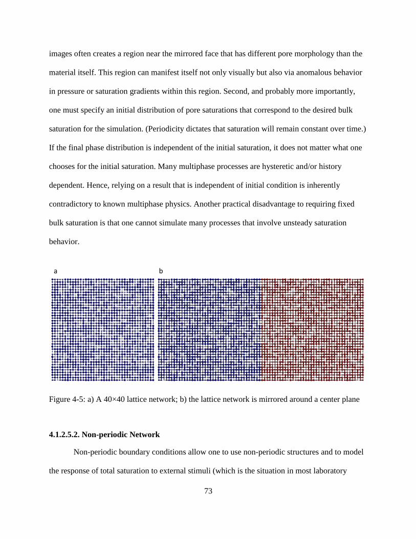
73

images often creates a region near the mirrored face that has different pore morphology than the

material itself. This region can manifest itself not only visually but also via anomalous behavior

in pressure or saturation gradients within this region. Second, and probably more importantly,

one must specify an initial distribution of pore saturations that correspond to the desired bulk

saturation for the simulation. (Periodicity dictates that saturation will remain constant over time.)

If the final phase distribution is independent of the initial saturation, it does not matter what one

chooses for the initial saturation. Many multiphase processes are hysteretic and/or history

dependent. Hence, relying on a result that is independent of initial condition is inherently

contradictory to known multiphase physics. Another practical disadvantage to requiring fixed

bulk saturation is that one cannot simulate many processes that involve unsteady saturation

behavior.

Figure 4-5: a) A 40×40 lattice network; b) the lattice network is mirrored around a center plane

4.1.2.5.2. Non-periodic Network

Non-periodic boundary conditions allow one to use non-periodic structures and to model

the response of total saturation to external stimuli (which is the situation in most laboratory

74

experiments or reservoir processes). Additionally, initial conditions are more likely to reflect a

known physical condition such as Sw = 0 or 1, or a residual saturation that can be estimated from

capillary pressure considerations. The tradeoff for these benefits is a more challenging set of

inlet/outlet boundary conditions.

A non-periodic network structure is defined to have inlet and outlet pores. These pores

can either lie directly on the inlet/outlet faces or lie inside the domain but have access to the

inlet/outlet face via connecting throats. (Whether a network will have one or the other or both

types of inlet/outlet connections is largely a matter of preference in defining network structure,

or it can depend on what type of data set the network comes from. It is mentioned here only to

note that it will affect nuts-and-bolts-level details of how the boundary conditions are

implemented.)

Generally, the inlet volumetric flow rates of wetting and non-wetting phases are specified

independently (or, equivalently, specify the total flow rate and fractional flow ratio). Unless the

specified inlet conditions are consistent with the current internal phase distribution, then a

transient period will be observed prior to reaching the steady state. At the steady state, the

saturation in every pore in the network is invariable with time. The boundary equations for a

non-periodic network are defined as follows:

innwinwinletnw

inlet

j nw

inletnwr

inwiwinletw

inlet

j w

inletwr

qppgg

qppgg

,,,

,

,,,

,

)(

)(

(4-12)

Two additional unknowns, inlet wetting-phase pressure pw,inlet and non-wetting-phase

pressure pnw,inlet, arise from the boundary conditions. At any given timestep, wetting phase

pressure and non-wetting phase pressure are assumed to be uniform for all inlet pores. The model

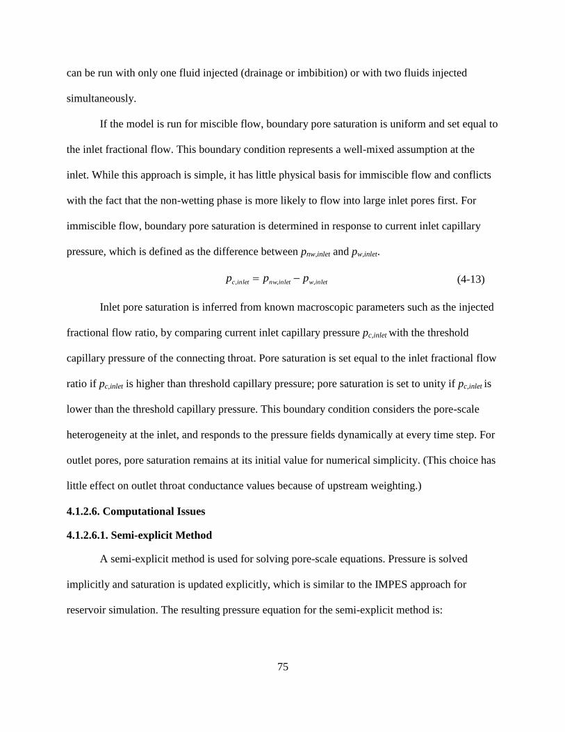
75

can be run with only one fluid injected (drainage or imbibition) or with two fluids injected

simultaneously.

If the model is run for miscible flow, boundary pore saturation is uniform and set equal to

the inlet fractional flow. This boundary condition represents a well-mixed assumption at the

inlet. While this approach is simple, it has little physical basis for immiscible flow and conflicts

with the fact that the non-wetting phase is more likely to flow into large inlet pores first. For

immiscible flow, boundary pore saturation is determined in response to current inlet capillary

pressure, which is defined as the difference between pnw,inlet and pw,inlet.

inletwinletnwinletc ppp ,,, (4-13)

Inlet pore saturation is inferred from known macroscopic parameters such as the injected

fractional flow ratio, by comparing current inlet capillary pressure pc,inlet with the threshold

capillary pressure of the connecting throat. Pore saturation is set equal to the inlet fractional flow

ratio if pc,inlet is higher than threshold capillary pressure; pore saturation is set to unity if pc,inlet is

lower than the threshold capillary pressure. This boundary condition considers the pore-scale

heterogeneity at the inlet, and responds to the pressure fields dynamically at every time step. For

outlet pores, pore saturation remains at its initial value for numerical simplicity. (This choice has

little effect on outlet throat conductance values because of upstream weighting.)

4.1.2.6. Computational Issues

4.1.2.6.1. Semi-explicit Method

A semi-explicit method is used for solving pore-scale equations. Pressure is solved

implicitly and saturation is updated explicitly, which is similar to the IMPES approach for

reservoir simulation. The resulting pressure equation for the semi-explicit method is:

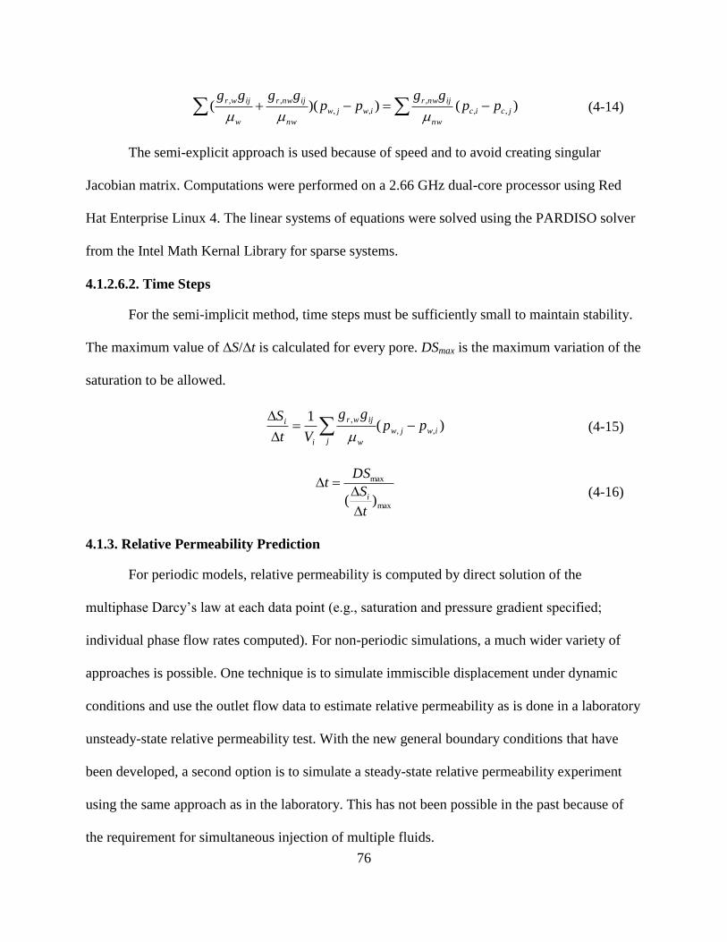
76

)())(( ,,

,

,,

,,

jcic

nw

ijnwr

iwjw

nw

ijnwr

w

ijwrpp

ggpp

gggg

(4-14)

The semi-explicit approach is used because of speed and to avoid creating singular

Jacobian matrix. Computations were performed on a 2.66 GHz dual-core processor using Red

Hat Enterprise Linux 4. The linear systems of equations were solved using the PARDISO solver

from the Intel Math Kernal Library for sparse systems.

4.1.2.6.2. Time Steps

For the semi-implicit method, time steps must be sufficiently small to maintain stability.

The maximum value of ∆S/∆t is calculated for every pore. DSmax is the maximum variation of the

saturation to be allowed.

)(1

,,

,

iwjw

j w

ijwr

i

i ppgg

Vt

S

(4-15)

max

max

)(t

S

DSt

i

(4-16)

4.1.3. Relative Permeability Prediction

For periodic models, relative permeability is computed by direct solution of the

multiphase Darcy’s law at each data point (e.g., saturation and pressure gradient specified;

individual phase flow rates computed). For non-periodic simulations, a much wider variety of

approaches is possible. One technique is to simulate immiscible displacement under dynamic

conditions and use the outlet flow data to estimate relative permeability as is done in a laboratory

unsteady-state relative permeability test. With the new general boundary conditions that have

been developed, a second option is to simulate a steady-state relative permeability experiment

using the same approach as in the laboratory. This has not been possible in the past because of

the requirement for simultaneous injection of multiple fluids.

77

To generate a steady-state relative permeability curve, the total flow rate and fractional

flow are specified, and both phases are injected from the inlet until a steady state is reached.

Relative permeability values for both phases are then calculated using the multiphase Darcy’s

law. The complete relative permeability curve is generated by repeatedly altering the injected

fractional flow, and waiting for the next steady state to evolve in a physically realistic way from

the previous state. More details on relative permeability prediction can be found in Chapter 5.

4.2. Results and Discussions

4.2.1. Permeability and Characteristic Scale

For the two image-based samples described in section 4.1, we ran a critical length finder

algorithm, which models single-phase, low-Reynolds number flow of a Newtonian fluid for

increasingly large subsections of the networks. For each sub-network, permeability is computed

by imposing a pressure gradient in the z direction and computing the resulting volumetric flow

rate. The characteristic scale for single-phase permeability for a material can be identified as the

point where small-length-scale oscillations die out. For the sandstone, we obtain a permeability

of 3.5-4.0 Darcy with a critical length of approximately 1.0 mm, as shown in Figure 4-6a. The

sand has a permeability of approximately 8.0-9.0 Darcy with a critical length of approximately

1.5 mm, as shown in Figure 4-6b.

4.2.2. Periodic Steady-state Simulation

Relative permeability curves were calculated using the steady-state method for both

periodic and non-periodic networks. We assumed uniform and strongly wetting surfaces (zero

degree contact angle) in all simulations.

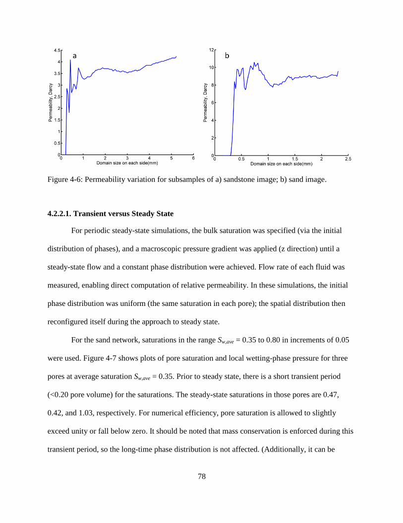
78

Figure 4-6: Permeability variation for subsamples of a) sandstone image; b) sand image.

4.2.2.1. Transient versus Steady State

For periodic steady-state simulations, the bulk saturation was specified (via the initial

distribution of phases), and a macroscopic pressure gradient was applied (z direction) until a

steady-state flow and a constant phase distribution were achieved. Flow rate of each fluid was

measured, enabling direct computation of relative permeability. In these simulations, the initial

phase distribution was uniform (the same saturation in each pore); the spatial distribution then

reconfigured itself during the approach to steady state.

For the sand network, saturations in the range Sw,ave = 0.35 to 0.80 in increments of 0.05

were used. Figure 4-7 shows plots of pore saturation and local wetting-phase pressure for three

pores at average saturation Sw,ave = 0.35. Prior to steady state, there is a short transient period

(<0.20 pore volume) for the saturations. The steady-state saturations in those pores are 0.47,

0.42, and 1.03, respectively. For numerical efficiency, pore saturation is allowed to slightly

exceed unity or fall below zero. It should be noted that mass conservation is enforced during this

transient period, so the long-time phase distribution is not affected. (Additionally, it can be

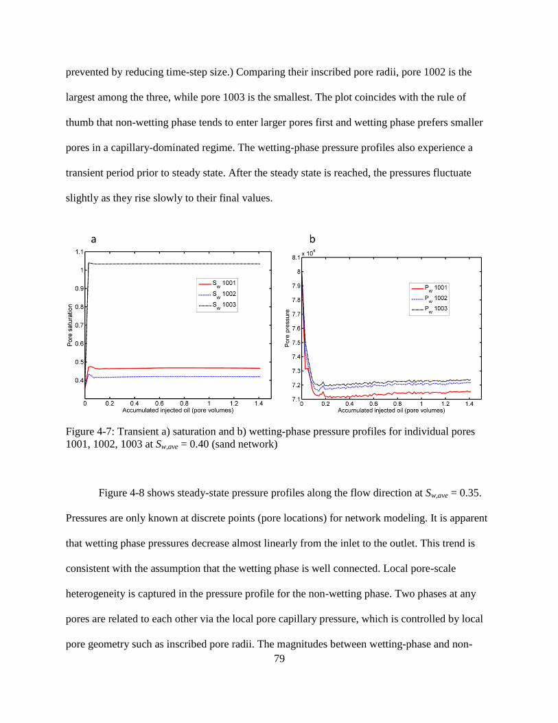
79

prevented by reducing time-step size.) Comparing their inscribed pore radii, pore 1002 is the

largest among the three, while pore 1003 is the smallest. The plot coincides with the rule of

thumb that non-wetting phase tends to enter larger pores first and wetting phase prefers smaller

pores in a capillary-dominated regime. The wetting-phase pressure profiles also experience a

transient period prior to steady state. After the steady state is reached, the pressures fluctuate

slightly as they rise slowly to their final values.

Figure 4-7: Transient a) saturation and b) wetting-phase pressure profiles for individual pores

1001, 1002, 1003 at Sw,ave = 0.40 (sand network)

Figure 4-8 shows steady-state pressure profiles along the flow direction at Sw,ave = 0.35.

Pressures are only known at discrete points (pore locations) for network modeling. It is apparent

that wetting phase pressures decrease almost linearly from the inlet to the outlet. This trend is

consistent with the assumption that the wetting phase is well connected. Local pore-scale

heterogeneity is captured in the pressure profile for the non-wetting phase. Two phases at any

pores are related to each other via the local pore capillary pressure, which is controlled by local

pore geometry such as inscribed pore radii. The magnitudes between wetting-phase and non-

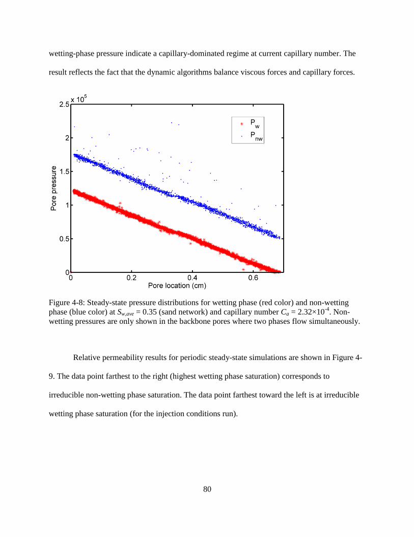
80

wetting-phase pressure indicate a capillary-dominated regime at current capillary number. The

result reflects the fact that the dynamic algorithms balance viscous forces and capillary forces.

Figure 4-8: Steady-state pressure distributions for wetting phase (red color) and non-wetting

phase (blue color) at Sw,ave = 0.35 (sand network) and capillary number Ca = 2.32×10-4

. Non-

wetting pressures are only shown in the backbone pores where two phases flow simultaneously.

Relative permeability results for periodic steady-state simulations are shown in Figure 4-

9. The data point farthest to the right (highest wetting phase saturation) corresponds to

irreducible non-wetting phase saturation. The data point farthest toward the left is at irreducible

wetting phase saturation (for the injection conditions run).

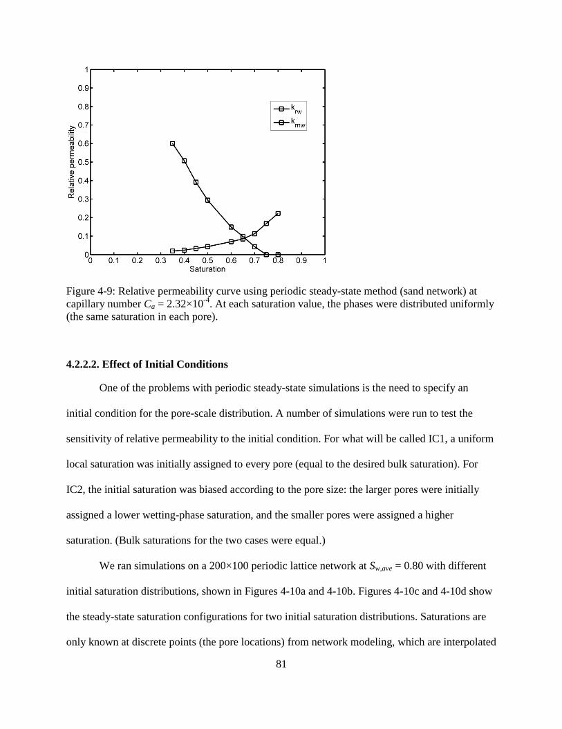
81

Figure 4-9: Relative permeability curve using periodic steady-state method (sand network) at

capillary number Ca = 2.32×10-4

. At each saturation value, the phases were distributed uniformly

(the same saturation in each pore).

4.2.2.2. Effect of Initial Conditions

One of the problems with periodic steady-state simulations is the need to specify an

initial condition for the pore-scale distribution. A number of simulations were run to test the

sensitivity of relative permeability to the initial condition. For what will be called IC1, a uniform

local saturation was initially assigned to every pore (equal to the desired bulk saturation). For

IC2, the initial saturation was biased according to the pore size: the larger pores were initially

assigned a lower wetting-phase saturation, and the smaller pores were assigned a higher

saturation. (Bulk saturations for the two cases were equal.)

We ran simulations on a 200×100 periodic lattice network at Sw,ave = 0.80 with different

initial saturation distributions, shown in Figures 4-10a and 4-10b. Figures 4-10c and 4-10d show

the steady-state saturation configurations for two initial saturation distributions. Saturations are

only known at discrete points (the pore locations) from network modeling, which are interpolated

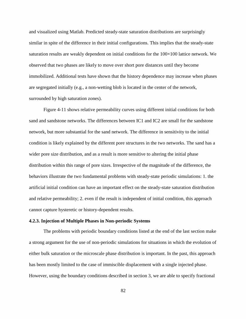
82

and visualized using Matlab. Predicted steady-state saturation distributions are surprisingly

similar in spite of the difference in their initial configurations. This implies that the steady-state

saturation results are weakly dependent on initial conditions for the 100×100 lattice network. We

observed that two phases are likely to move over short pore distances until they become

immobilized. Additional tests have shown that the history dependence may increase when phases

are segregated initially (e.g., a non-wetting blob is located in the center of the network,

surrounded by high saturation zones).

Figure 4-11 shows relative permeability curves using different initial conditions for both

sand and sandstone networks. The differences between IC1 and IC2 are small for the sandstone

network, but more substantial for the sand network. The difference in sensitivity to the initial

condition is likely explained by the different pore structures in the two networks. The sand has a

wider pore size distribution, and as a result is more sensitive to altering the initial phase

distribution within this range of pore sizes. Irrespective of the magnitude of the difference, the

behaviors illustrate the two fundamental problems with steady-state periodic simulations: 1. the

artificial initial condition can have an important effect on the steady-state saturation distribution

and relative permeability; 2. even if the result is independent of initial condition, this approach

cannot capture hysteretic or history-dependent results.

4.2.3. Injection of Multiple Phases in Non-periodic Systems

The problems with periodic boundary conditions listed at the end of the last section make

a strong argument for the use of non-periodic simulations for situations in which the evolution of

either bulk saturation or the microscale phase distribution is important. In the past, this approach

has been mostly limited to the case of immiscible displacement with a single injected phase.

However, using the boundary conditions described in section 3, we are able to specify fractional

83

flow at the inlet, simulating the incremental changes in saturation that would be seen in certain

reservoir situations or in a steady-state relative permeability test.

Figure 4-10: Saturation distributions at average Sw,ave = 0.8 in a 100×100 lattice network. a) IC1,

uniform initial saturation; b) IC2, biased initial saturation distribution; c) steady-state saturation

distribution for IC1; d) steady-state saturation distribution for IC2. Simulations are run on a

200×100 periodic lattice network (by mirroring a 100×100 lattice network). Only the original

100×100 lattice network is used for saturation visualization.

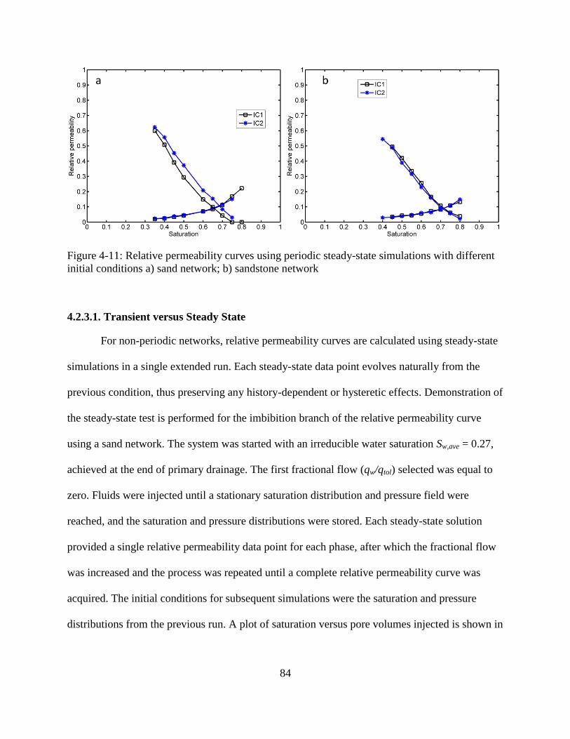
84

Figure 4-11: Relative permeability curves using periodic steady-state simulations with different

initial conditions a) sand network; b) sandstone network

4.2.3.1. Transient versus Steady State

For non-periodic networks, relative permeability curves are calculated using steady-state

simulations in a single extended run. Each steady-state data point evolves naturally from the

previous condition, thus preserving any history-dependent or hysteretic effects. Demonstration of

the steady-state test is performed for the imbibition branch of the relative permeability curve

using a sand network. The system was started with an irreducible water saturation Sw,ave = 0.27,

achieved at the end of primary drainage. The first fractional flow (qw/qtol) selected was equal to

zero. Fluids were injected until a stationary saturation distribution and pressure field were

reached, and the saturation and pressure distributions were stored. Each steady-state solution

provided a single relative permeability data point for each phase, after which the fractional flow

was increased and the process was repeated until a complete relative permeability curve was

acquired. The initial conditions for subsequent simulations were the saturation and pressure

distributions from the previous run. A plot of saturation versus pore volumes injected is shown in

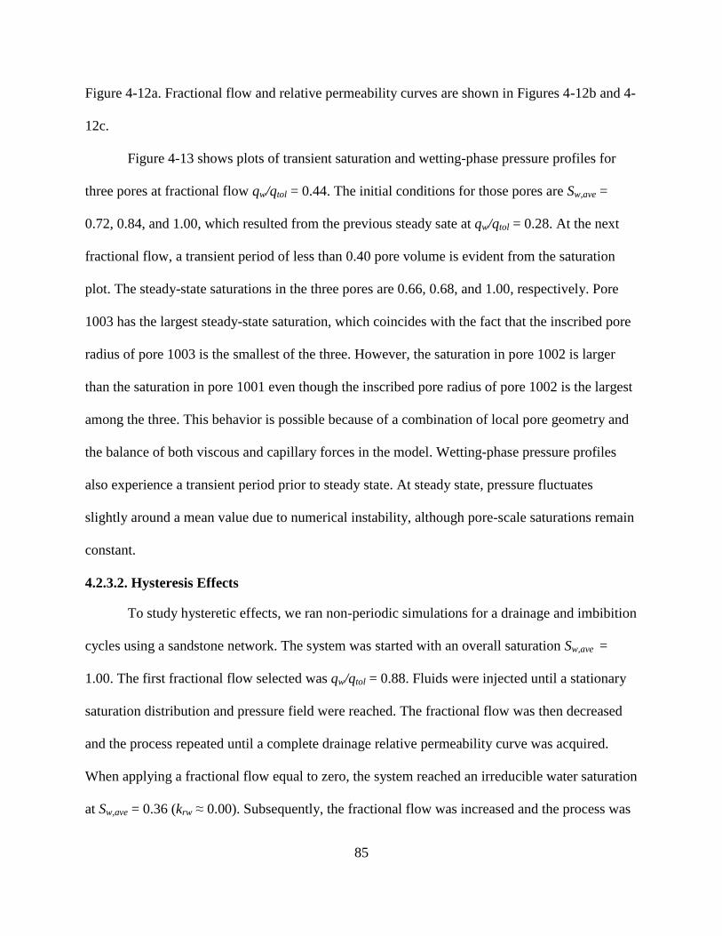
85

Figure 4-12a. Fractional flow and relative permeability curves are shown in Figures 4-12b and 4-

12c.

Figure 4-13 shows plots of transient saturation and wetting-phase pressure profiles for

three pores at fractional flow qw/qtol = 0.44. The initial conditions for those pores are Sw,ave =

0.72, 0.84, and 1.00, which resulted from the previous steady sate at qw/qtol = 0.28. At the next

fractional flow, a transient period of less than 0.40 pore volume is evident from the saturation

plot. The steady-state saturations in the three pores are 0.66, 0.68, and 1.00, respectively. Pore

1003 has the largest steady-state saturation, which coincides with the fact that the inscribed pore

radius of pore 1003 is the smallest of the three. However, the saturation in pore 1002 is larger

than the saturation in pore 1001 even though the inscribed pore radius of pore 1002 is the largest

among the three. This behavior is possible because of a combination of local pore geometry and

the balance of both viscous and capillary forces in the model. Wetting-phase pressure profiles

also experience a transient period prior to steady state. At steady state, pressure fluctuates

slightly around a mean value due to numerical instability, although pore-scale saturations remain

constant.

4.2.3.2. Hysteresis Effects

To study hysteretic effects, we ran non-periodic simulations for a drainage and imbibition

cycles using a sandstone network. The system was started with an overall saturation Sw,ave =

1.00. The first fractional flow selected was qw/qtol = 0.88. Fluids were injected until a stationary

saturation distribution and pressure field were reached. The fractional flow was then decreased

and the process repeated until a complete drainage relative permeability curve was acquired.

When applying a fractional flow equal to zero, the system reached an irreducible water saturation

at Sw,ave = 0.36 (krw ≈ 0.00). Subsequently, the fractional flow was increased and the process was

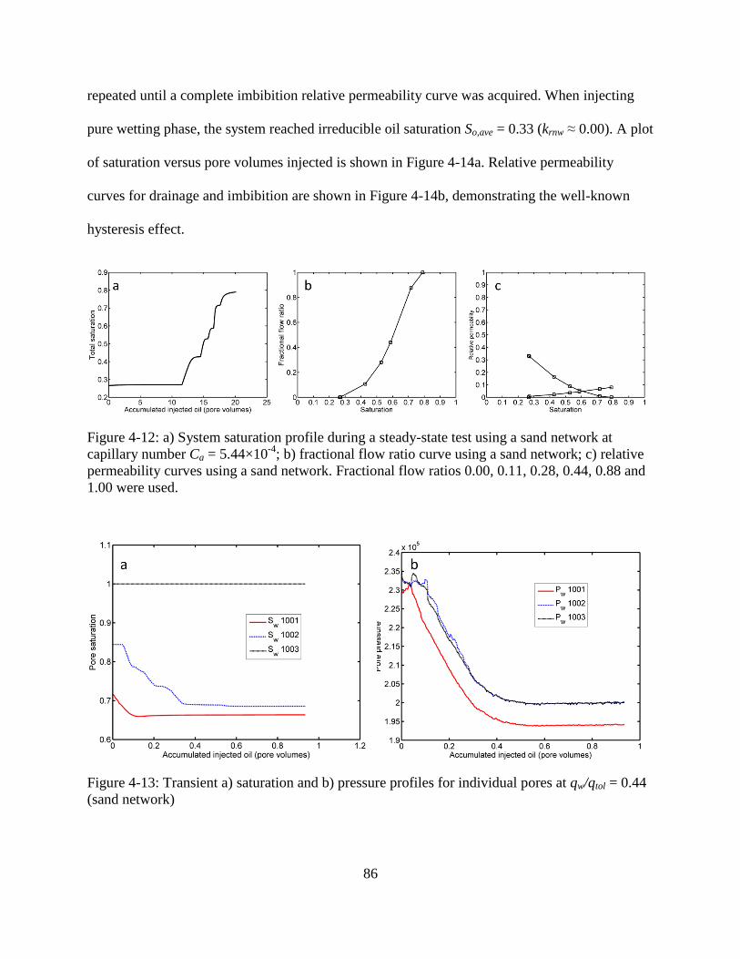
86

repeated until a complete imbibition relative permeability curve was acquired. When injecting

pure wetting phase, the system reached irreducible oil saturation So,ave = 0.33 (krnw ≈ 0.00). A plot

of saturation versus pore volumes injected is shown in Figure 4-14a. Relative permeability

curves for drainage and imbibition are shown in Figure 4-14b, demonstrating the well-known

hysteresis effect.

Figure 4-12: a) System saturation profile during a steady-state test using a sand network at

capillary number Ca = 5.44×10-4

; b) fractional flow ratio curve using a sand network; c) relative

permeability curves using a sand network. Fractional flow ratios 0.00, 0.11, 0.28, 0.44, 0.88 and

1.00 were used.

Figure 4-13: Transient a) saturation and b) pressure profiles for individual pores at qw/qtol = 0.44

(sand network)

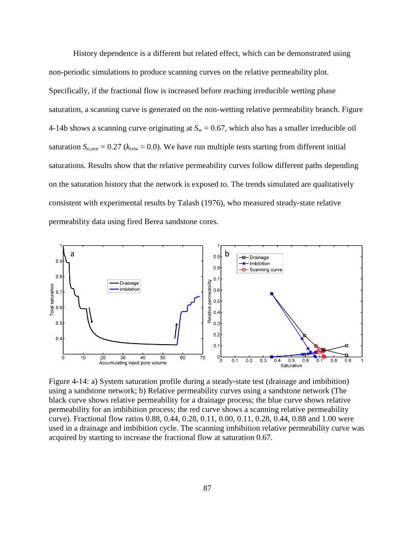
87

History dependence is a different but related effect, which can be demonstrated using

non-periodic simulations to produce scanning curves on the relative permeability plot.

Specifically, if the fractional flow is increased before reaching irreducible wetting phase

saturation, a scanning curve is generated on the non-wetting relative permeability branch. Figure

4-14b shows a scanning curve originating at Sw = 0.67, which also has a smaller irreducible oil

saturation So,ave = 0.27 (krnw ≈ 0.0). We have run multiple tests starting from different initial

saturations. Results show that the relative permeability curves follow different paths depending

on the saturation history that the network is exposed to. The trends simulated are qualitatively

consistent with experimental results by Talash (1976), who measured steady-state relative

permeability data using fired Berea sandstone cores.

Figure 4-14: a) System saturation profile during a steady-state test (drainage and imbibition)

using a sandstone network; b) Relative permeability curves using a sandstone network (The

black curve shows relative permeability for a drainage process; the blue curve shows relative

permeability for an imbibition process; the red curve shows a scanning relative permeability

curve). Fractional flow ratios 0.88, 0.44, 0.28, 0.11, 0.00, 0.11, 0.28, 0.44, 0.88 and 1.00 were

used in a drainage and imbibition cycle. The scanning imbibition relative permeability curve was

acquired by starting to increase the fractional flow at saturation 0.67.

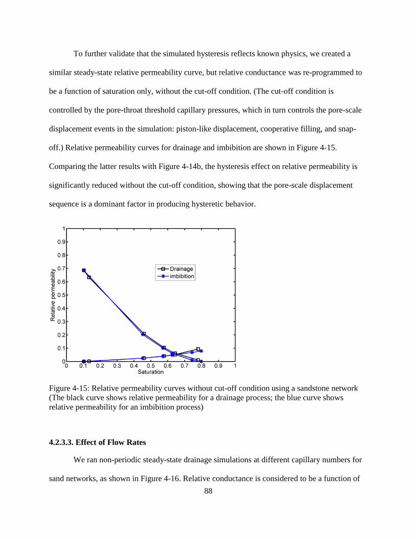
88

To further validate that the simulated hysteresis reflects known physics, we created a

similar steady-state relative permeability curve, but relative conductance was re-programmed to

be a function of saturation only, without the cut-off condition. (The cut-off condition is

controlled by the pore-throat threshold capillary pressures, which in turn controls the pore-scale

displacement events in the simulation: piston-like displacement, cooperative filling, and snap-

off.) Relative permeability curves for drainage and imbibition are shown in Figure 4-15.

Comparing the latter results with Figure 4-14b, the hysteresis effect on relative permeability is

significantly reduced without the cut-off condition, showing that the pore-scale displacement

sequence is a dominant factor in producing hysteretic behavior.

Figure 4-15: Relative permeability curves without cut-off condition using a sandstone network

(The black curve shows relative permeability for a drainage process; the blue curve shows

relative permeability for an imbibition process)

4.2.3.3. Effect of Flow Rates

We ran non-periodic steady-state drainage simulations at different capillary numbers for

sand networks, as shown in Figure 4-16. Relative conductance is considered to be a function of

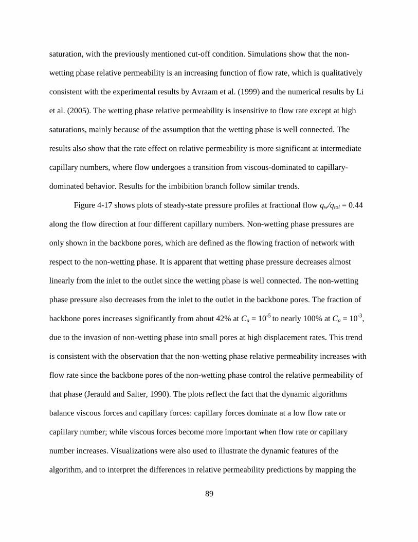
89

saturation, with the previously mentioned cut-off condition. Simulations show that the non-

wetting phase relative permeability is an increasing function of flow rate, which is qualitatively

consistent with the experimental results by Avraam et al. (1999) and the numerical results by Li

et al. (2005). The wetting phase relative permeability is insensitive to flow rate except at high

saturations, mainly because of the assumption that the wetting phase is well connected. The

results also show that the rate effect on relative permeability is more significant at intermediate

capillary numbers, where flow undergoes a transition from viscous-dominated to capillary-

dominated behavior. Results for the imbibition branch follow similar trends.

Figure 4-17 shows plots of steady-state pressure profiles at fractional flow qw/qtol = 0.44

along the flow direction at four different capillary numbers. Non-wetting phase pressures are

only shown in the backbone pores, which are defined as the flowing fraction of network with

respect to the non-wetting phase. It is apparent that wetting phase pressure decreases almost

linearly from the inlet to the outlet since the wetting phase is well connected. The non-wetting

phase pressure also decreases from the inlet to the outlet in the backbone pores. The fraction of

backbone pores increases significantly from about 42% at Ca = 10-5

to nearly 100% at Ca = 10-3

,

due to the invasion of non-wetting phase into small pores at high displacement rates. This trend

is consistent with the observation that the non-wetting phase relative permeability increases with

flow rate since the backbone pores of the non-wetting phase control the relative permeability of

that phase (Jerauld and Salter, 1990). The plots reflect the fact that the dynamic algorithms

balance viscous forces and capillary forces: capillary forces dominate at a low flow rate or

capillary number; while viscous forces become more important when flow rate or capillary

number increases. Visualizations were also used to illustrate the dynamic features of the

algorithm, and to interpret the differences in relative permeability predictions by mapping the

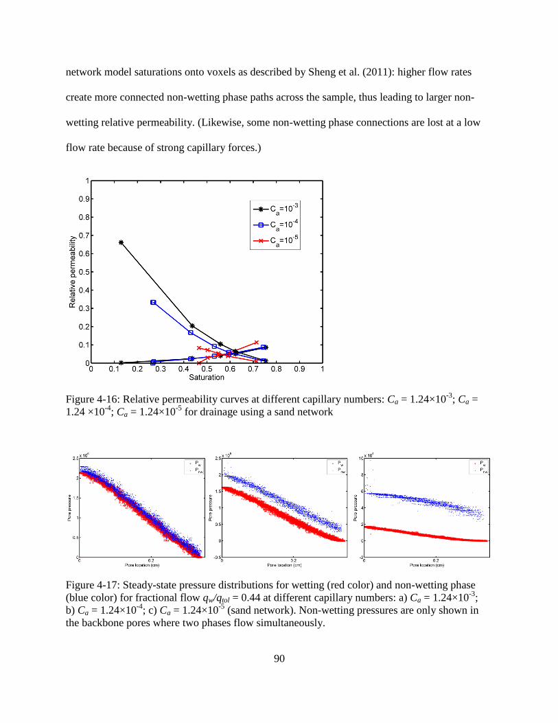
90

network model saturations onto voxels as described by Sheng et al. (2011): higher flow rates

create more connected non-wetting phase paths across the sample, thus leading to larger non-

wetting relative permeability. (Likewise, some non-wetting phase connections are lost at a low

flow rate because of strong capillary forces.)

Figure 4-16: Relative permeability curves at different capillary numbers: Ca = 1.24×10-3

; Ca =

1.24 ×10-4

; Ca = 1.24×10-5

for drainage using a sand network

Figure 4-17: Steady-state pressure distributions for wetting (red color) and non-wetting phase

(blue color) for fractional flow qw/qtol = 0.44 at different capillary numbers: a) Ca = 1.24×10-3

;

b) Ca = 1.24×10-4

; c) Ca = 1.24×10-5

(sand network). Non-wetting pressures are only shown in

the backbone pores where two phases flow simultaneously.

91

4.2.3.4. Effect of Fractional Flow Ratios and Viscosity Ratios

We ran non-periodic steady-state drainage simulations at three viscosity ratios (0.1, 1 and

30) and two fractional flow ratios (0.0 and 0.5) on a 100×100 lattice network. For fractional flow

ratio equal to zero, figures 4-18a, 4-18b and 4-18c show transient saturation configurations at

saturation Sw,ave = 0.80, visualized using Matlab. For fractional flow ratio equal to 0.5, figures 4-

18d, 4-18e and 4-18f show transient saturation distributions at saturation Sw,ave = 0.63. The case

of zero fractional flow ratio is equivalent to the injection of the non-wetting phase only. For this

case, predicted saturation distributions are characteristic of viscous fingering at low viscosity

ratios, and experienced a continuous transition from viscous fingering to stable displacement

when viscosity ratios were increased. This observation agrees well with the experimental results

by Lenormand et al. (1988) in micro-models. With respect to the case of fractional flow ratio 0.5,

the saturation distributions experienced a continuous transition from viscous fingering to stable

displacement for increasing viscosity ratios. We noted that each phase was likely to move

through its segregated flow channels for this case, which leads to a gradual change in saturation

gradient and a smearing front. Different flow patterns for different fractional ratios are also

observed for a sandstone network, as shown in Figure 4-19.

4.2.3.5. Effect of Thick Wetting Films

We examined the sensitivity of relative permeability function to one of the critical

parameters in the network model: the resistance factor β (which controls hydraulic conductance

in the thick wetting films), and whether relative permeability curves shift in the correct direction

as resistance factor is varied. This particular parameter is a subject of particular interest because

it has a somewhat tenuous connection to pore-throat and wetting-phase geometries in real porous

media, and likely would benefit from further research.

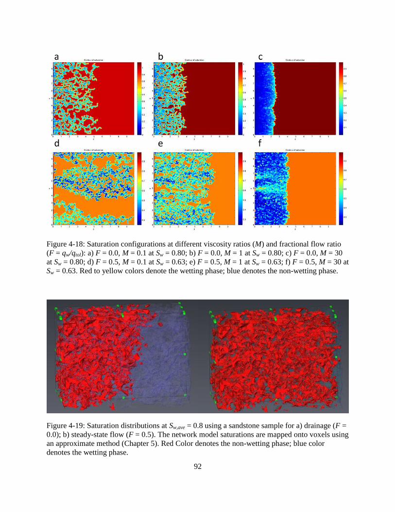
92

Figure 4-18: Saturation configurations at different viscosity ratios (M) and fractional flow ratio

(F = qw/qtol): a) F = 0.0, M = 0.1 at Sw = 0.80; b) F = 0.0, M = 1 at Sw = 0.80; c) F = 0.0, M = 30

at Sw = 0.80; d) F = 0.5, M = 0.1 at Sw = 0.63; e) F = 0.5, M = 1 at Sw = 0.63; f) F = 0.5, M = 30 at

Sw = 0.63. Red to yellow colors denote the wetting phase; blue denotes the non-wetting phase.

Figure 4-19: Saturation distributions at Sw,ave = 0.8 using a sandstone sample for a) drainage (F =

0.0); b) steady-state flow (F = 0.5). The network model saturations are mapped onto voxels using

an approximate method (Chapter 5). Red Color denotes the non-wetting phase; blue color

denotes the wetting phase.

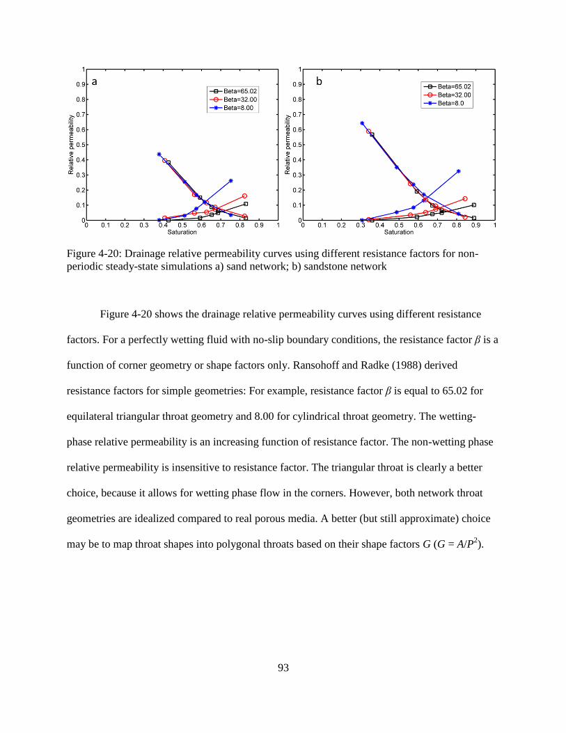
93

Figure 4-20: Drainage relative permeability curves using different resistance factors for non-

periodic steady-state simulations a) sand network; b) sandstone network

Figure 4-20 shows the drainage relative permeability curves using different resistance

factors. For a perfectly wetting fluid with no-slip boundary conditions, the resistance factor β is a

function of corner geometry or shape factors only. Ransohoff and Radke (1988) derived

resistance factors for simple geometries: For example, resistance factor β is equal to 65.02 for

equilateral triangular throat geometry and 8.00 for cylindrical throat geometry. The wetting-

phase relative permeability is an increasing function of resistance factor. The non-wetting phase

relative permeability is insensitive to resistance factor. The triangular throat is clearly a better

choice, because it allows for wetting phase flow in the corners. However, both network throat

geometries are idealized compared to real porous media. A better (but still approximate) choice

may be to map throat shapes into polygonal throats based on their shape factors G (G = A/P2).

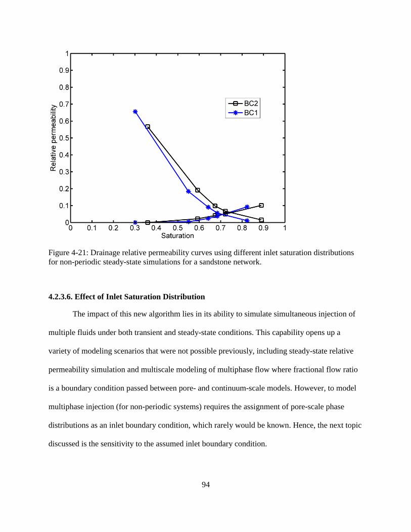
94

Figure 4-21: Drainage relative permeability curves using different inlet saturation distributions

for non-periodic steady-state simulations for a sandstone network.

4.2.3.6. Effect of Inlet Saturation Distribution

The impact of this new algorithm lies in its ability to simulate simultaneous injection of

multiple fluids under both transient and steady-state conditions. This capability opens up a

variety of modeling scenarios that were not possible previously, including steady-state relative

permeability simulation and multiscale modeling of multiphase flow where fractional flow ratio

is a boundary condition passed between pore- and continuum-scale models. However, to model

multiphase injection (for non-periodic systems) requires the assignment of pore-scale phase

distributions as an inlet boundary condition, which rarely would be known. Hence, the next topic

discussed is the sensitivity to the assumed inlet boundary condition.

95

Simulations were performed using two different inlet boundary conditions. In the first

approach, saturations of all inlet pores were set equal to the overall inlet fractional flow (BC1).

This is a convenient simplification but is not physically realistic. In the second approach,

saturations were assigned by comparing current inlet capillary pressure Pc,inlet with the threshold

capillary pressure of the connecting throat (BC2), as described in section 4.1. This BC is

analagous to what is used for immiscible displcement algorithms, and more accurately reflects

the pore-scale physics.

The drainage relative permeability profiles show different behaviors using the two

boundary conditions, as shown in Figure 4-21. This result demonstrates that the inlet saturation

distribution affects details of the pore-scale distribution of phases at steady-state conditions, and

therefore the corresponding relative permeability values. For the sandstone network used here,

the non-wetting-phase relative permeability is larger with the more realistic boundary condition

BC2, while wetting-phase relative permeability is insensitive to the inlet saturation distribution.

The likely reason for this behavior is that coupling the inlet condition to the capillary entry

pressure allows the non-wetting phase to flow into a set of larger pores rather than being

distributed more uniformly throughout the pore space.

4.2.4. Periodic versus Non-periodic Steady-state Simulation

The use of periodic boundary conditions allows one to avoid the boundary condition

issues discussed in the previous section. However, it prevents the simulation of processes where

saturation changes over time. Figure 4-22 combines plots of relative permeability for periodic

versus non-periodic steady-state simulations, applied to sand or sandstone networks. For periodic

steady-state simulation, the phases were distributed uniformly (the same saturation in each pore)

at each saturation value. Results from the two steady-state techniques (periodic and non-

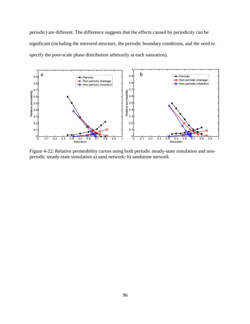
96

periodic) are different. The difference suggests that the effects caused by periodicity can be

significant (including the mirrored structure, the periodic boundary conditions, and the need to

specify the pore-scale phase distribution arbitrarily at each saturation).

Figure 4-22: Relative permeability curves using both periodic steady-state simulation and non-

periodic steady-state simulation a) sand network; b) sandstone network

97

5. Numerical Prediction of Relative Permeability2

Numerical prediction of rock properties is a rapidly evolving area that has the potential to

influence dramatically how core analysis is performed. Of these various properties, relative

permeability is one of the most important both because of its role in reservoir simulation and

because of the experimental challenges, including the time associated with laboratory

measurements.

In this chapter, the numerical prediction of relative permeability from micro-computed

tomographic images is investigated using pore network modeling. Specifically, four different

algorithms are applied to a digital image of a reservoir sample that has been tested using

traditional core analysis, and compare the results.

5.1. Core Samples and Network Generation

5.1.1. Core Samples

Three “twinned” plugs were taken from a core recovered from a sandstone reservoir, with

the three plugs all coming from the exact same depth interval. Two of the plugs were used in

unsteady-state laboratory corefloods performed at two different flow rates. A small “mini-core”

was extracted from the third plug and used for microCT imaging. The porosity and equivalent

liquid permeability measured on one plug using routine core analysis were 31% and 2.0 Darcy,

respectively.

5.1.2. MicroCT Imaging

The microCT image was used to extract a rectangular domain with dimensions

1024×1024×1484 that contained only the sample, and processed to obtain a two-phase

2 Chapter 5 is originally presented in SPE ATCE Conference in Oct 2011, Denver, CO.

98

description containing voxels identified as either pore or solid. The physical dimension of the

voxels is 3.52 micron.

5.1.3. Network Generation

The network is constructed from the segmented microCT image using an algorithm

described in detail elsewhere (Thompson et al. 2008; Bhattad et al. 2011). In short, the locations

of maximal inscribed spheres are found using a nonlinear optimization process. The center of

each inscribed sphere is assigned as a pore location. The pore itself (shape and volume) is

defined by a cluster of voxels surrounding each pore center. The voxels are collected using a

watershed-type algorithm that tags each voxel with the pore to which it belongs and also ensures

that two growing clusters of voxels meet at the smallest constriction between the two pores.

Accordingly, the boundary between two clusters of voxels (each tagged with a different pore

number) defines a pore throat. A search for these boundaries defines the connectivity of the

network. Once the pore locations and connectivity are defined, direct geometric analysis is used

to compute remaining geometric properties used in the network description: pore volume,

surface area, pore inscribed radius, throat inscribed radius, throat cross-sectional area, and throat

wetted perimeter.

The hydraulic conductance of each pore throat must be known in order to compute

permeability and relative permeability. It is determined by approximating the throat geometry as

a duct for which an analytic or empirical formula for viscous flow exists. Many different

conductance formulas have been used, ranging from simple capillary tubes to orifices to Venturi

tubes to non-circular ducts. The use of different formulas for hydraulic conductance will

generally result in different permeability values and pore-scale flow distributions; hence, without

direct calibration for a specific sample or type of structure (e.g., using a CFD model), this choice

99

is somewhat arbitrary. We use a formula for low-Reynolds number flow through a Venturi tube,

which has been adapted to use the parameters extracted during the network generation step

(Thompson et al., 2008; Bhattad et al., 2011). It has been validated for uniform packings of

spheres using LBM results, but generally over predicts the permeability of consolidated

materials.

Depending on the algorithm, certain parameters associated with multiphase flow can be

determined a priori as part of the network generation step. Alternatively, they are treated as

dynamic parameters that must be computed in the flow modeling part. In principle, pore capillary

pressure should be a dynamically computed parameter because it exhibits a history dependence

related to the specific location of the interfaces in the pore. However, in the context of network

modeling, this relationship is usually simplified so that capillary pressure in a pore is a single-

valued function of the local phase saturation and the pore structure. In the current model, pore

capillary pressures are approximated using functionality for a cube-shaped pore but mapped onto

the individual network pores using additional geometric information (Thompson, 2002). The

other parameter worth mentioning is the conductance of an individual phase in a pore throat.

This parameter is defined as a non-dimensional multiplier of the absolute hydraulic conductance

of the throat (analogous to how relative permeability operates on absolute permeability). The

phase conductance values are determined using geometric information for the pore throats along

with local saturation. Because saturation is a pore property in our implementation, we employ an

upstream weighting scheme for the pore-throat phase conductance, which makes it a dynamic

parameter computed during the flow modeling.

100

5.2. Network Modeling of Relative Permeability

5.2.1. Quasi-static Method (QS)

Quasi-static drainage is performed by prescribing an applied capillary pressure and then

searching over all interface positions to locate pore-throats where the capillary entry pressure

allows the non-wetting phase to advance. When no further invasion is possible, a static

equilibrium has been reached and the capillary pressure must be increased to force the non-

wetting front to advance further. Because the displacement is quasi-static, the pressure in each

phase (and therefore the capillary pressure) is spatially uniform. However, the phase saturation in

each invaded pore is distinct and depends on the current capillary pressure because as capillary

pressure increases, interfaces squeeze deeper into corners and crevices and the non-wetting phase

saturation decreases. This behavior is quantified by the pore-capillary-pressure function, which

depends strongly on pore geometry and wettability (and on the specific menisci locations if the

function is designed to account for this effect). We assume zero-degree contact angles

everywhere and restrict the quasi-static simulations to drainage, which reduces the number of

different types of interface configurations that must be accounted for. The overall saturation in

the network at a given capillary pressure is determined by summing the total wetting and non-

wetting-phase volumes in each pore.

When static equilibrium has been reached for any given capillary pressure, relative

permeability is computed by performing two independent single-phase flow simulations in the

wetting and non-wetting phases. Clearly, the non-wetting phase displacement must have reached

the outlet in order to perform a flow simulation in that phase. This fact limits the range of

saturation values over which non-wetting phase relative permeability can be determined. It also

exposes one of the significant weaknesses (related to non-physical behavior) of this approach.

101

5.2.2. Unsteady-state Method during a Dynamic Displacement Process (USS)

This approach is intended to mimic laboratory unsteady-state relative permeability tests:

transient data from a two-phase displacement simulation is used to determine relative

permeability. The displacement simulations use a dynamic multiphase algorithm, so that both

viscous and capillary forces are accounted for.

The specific procedure is the following. The system is initially saturated with wetting

phase. Non-wetting phase fluid is injected from the inlet to displace the wetting phase at a

constant flow rate. (In some cases, a small amount of wetting phase is also injected, in which

case the fractional flow is also specified.) After obtaining the transient displacement data, a

graphical method similar to Jones and Roszelle (1978) is used to plot average oil saturation and

average effective viscosity during drainage. The oil saturation at the outlet is obtained from the

intercept value (ordinate axis) of the tangent line in the average saturation curve. We also use the

identical method for effective viscosity at the outlet. Outlet flow rate ratios and relative

permeability for each phase is calculated based on Buckley-Leverett theory. We have also

implemented the equivalent procedure but for imbibition.

5.2.3. Steady-state Method Using a Periodic Network (SSP)

Steady-state simulations provide the most direct route to relative permeability

computation because all parameters in the multiphase Darcy’s equation except for relative

permeability are directly from the model. Additionally, assuming the simulations use a dynamic

algorithm, this approach corresponds most closely to the physics implied by the equation. The

difficulty is that this approach requires an algorithm that can accommodate the simultaneous

injection of more than one fluid (as opposed to a traditional immiscible displacement algorithm).

For pore-scale network models this approach presents a significant problem when assigning

102

boundary conditions because the pore saturations and local capillary pressures must be assigned

individually for every inlet pore and this information cannot be obtained from known

macroscopic parameters such as overall fractional flow. One way to avoid this problem is to

employ periodic boundary conditions because the required inlet information can then be obtained

from the periodic outlet. This procedure is relatively straightforward, but it involves compromise

for two reasons. First, it requires a periodic structure, meaning the network must be artificial

(e.g., a lattice network) or a tomography-based network that has been mirrored in the flow

direction. Second, and more significant, is that saturation must be specified (as opposed to the

injected fractional flow) because periodicity dictates that saturation will remain constant over

time. For a pore-scale model, specifying bulk saturation means specifying the pore-scale

saturation distribution as an initial condition, which in turn implies that either (1) it is known for

real systems, or (2) a unique relative permeability exists for every global saturation value,

independent of the distributed initial condition. Neither of these statements is easily defensible

for systems we are interested in.

Despite the above mentioned shortcomings, the periodic steady-state approach has

important advantages, which is why we will present results separately from the non-periodic

steady-state approach. For tomography-based networks, we mirror the network structure in the

direction of flow, and two-phase flow is simulated as follows. Both phases are distributed within

the pore space such that the total saturation corresponds to a specified value. (A number of

approaches can be designed for deciding the spatial distribution, as discussed briefly in the

results.) No-flow boundary conditions are imposed along the non-inlet/outlet faces. Flow is

induced by incorporating a body force term in the governing equations or by imposing a total

flow rate through the network. In the current algorithm we use the latter approach, which means

103

that the overall pressure gradient becomes an unknown that is obtained by solution of the

network model. Once a steady-state is reached, and the pore-scale distribution of phases is

unchanging, relative permeability is computed by direct solution of the multiphase Darcy’s law.

5.2.4. Steady-state Method Using a Non-periodic Network (SSN)

Steady-state simulations in non-periodic networks closely mimic steady-state coreflood

tests in the laboratory. Computationally, they avoid the major problem with periodic simulations

because they typically begin with a known (and physically realistic) saturation distribution. Two

common starting points would be either fully saturated with one phase or a residual saturation

(which could be determined from a displacement simulation). From this starting point, the pore-

scale saturation distribution evolves over time in accordance with the governing equations and

depending on the selected flow rate and fractional flow ratio. As explained in the previous

section, the major problem that has prevented this approach from being used in the past is

inferring inlet pore-scale boundary conditions from known macroscopic parameters such as the

injected fractional flow ratio. We use a new algorithm to overcome this problem, which is

detailed in Chapter 4. In short, internal dynamic pore-throat parameters such as phase

conductance values are computed using upstream weighting. At the entrance, where upstream

weighting is not possible, the pore saturation is determined in response to the current inlet

capillary pressure, which is defined as the difference between inlet non-wetting phase pressure

and inlet wetting phase pressure. (Both can be obtained from solution of the network model.)

For primary drainage simulations, the system begins saturated with wetting phase. For

secondary drainage, irreducible non-wetting phase is present in the system initially. Total flow

rate and fractional flow are specified, and both phases are injected from the inlet until a steady

state is reached (determined by a stationary saturation and pressure distribution). Relative

104

permeability for each phase is then calculated using Darcy’s law. To complete the relative

permeability curve, the injected fractional flow (qw/qtot) is decreased, and the next steady state

evolves in a physically realistic way from the previous one. Note that this approach eliminates

the need to specify initial pore-scale saturations, which is the main problem with the periodic

simulations. An analogous simulation can be performed starting with Snw = 1 and incrementally

increasing the injected fractional flow.

5.2.5. Phase Saturation Distributions

Visual inspection of pore-scale phase distributions can be invaluable for interpreting

relative permeability behavior. Unfortunately, visualization is difficult with network modeling

because the phase distributions within specific pores are not solved for explicitly (as they would

be with LBM for instance), visual depictions of network structures are abstract, and 3D

disordered networks are difficult to visualize on paper. Consequently, we developed a simple

algorithm to map pore-scale network saturations onto voxels in the original tomography image.

Fluid distributions can then be visualized using 2D slices from the image. The algorithm is not

meant to produce quantitative sub-pore-scale fluid distributions, but is valuable for interpreting

differences between one algorithm and another.

The process of creating these visualizations is the following. During the network

generation step, every void voxel in the CT image is assigned to one of the network pores.

Additionally, each voxel in the image can be assigned a value from an approximate distance

map, obtained via a burn or erosion of the pore space. This value approximates the distance to

the nearest surface. To create the sub-pore-scale phase distributions, voxels closest to the surface

in a given pore are populated with wetting phase, and this process continues until the saturation

in that pore has reached the corresponding saturation in the network model. Non-wetting phase is

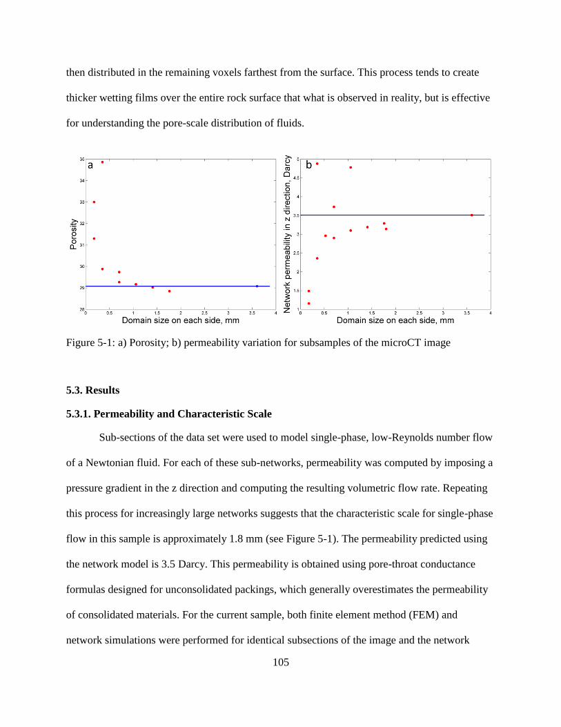
105

then distributed in the remaining voxels farthest from the surface. This process tends to create

thicker wetting films over the entire rock surface that what is observed in reality, but is effective

for understanding the pore-scale distribution of fluids.

Figure 5-1: a) Porosity; b) permeability variation for subsamples of the microCT image

5.3. Results

5.3.1. Permeability and Characteristic Scale

Sub-sections of the data set were used to model single-phase, low-Reynolds number flow

of a Newtonian fluid. For each of these sub-networks, permeability was computed by imposing a

pressure gradient in the z direction and computing the resulting volumetric flow rate. Repeating

this process for increasingly large networks suggests that the characteristic scale for single-phase

flow in this sample is approximately 1.8 mm (see Figure 5-1). The permeability predicted using

the network model is 3.5 Darcy. This permeability is obtained using pore-throat conductance

formulas designed for unconsolidated packings, which generally overestimates the permeability

of consolidated materials. For the current sample, both finite element method (FEM) and

network simulations were performed for identical subsections of the image and the network

106

model consistently overestimated the FEM simulations by 30%. Adjusting the network results

accordingly suggests that the permeability of the full 1024×1024×1484 image is about 2.7 Darcy.

This value is not inconsistent with the 2.0 Darcy permeability of the larger core sample: the

permeability of a three-mm digital section can be either smaller or larger than a laboratory-size

coreplug depending on spatial heterogeneity in the material. The relative permeability algorithms

were tested using a range of absolute conductance formulas (which produced a three-fold range

of absolute permeability), and this choice had little effect on the computed relative permeability.

Hence, no adjustment was made to the absolute permeability of the network when running the

simulations shown below. Results shown in this Chapter are from a 5123 voxel section of the

image unless otherwise stated. This corresponds to a cube 1.8 mm on each side. It contains

21,073 pores, approximately one tenth of the number of pores in the network from the full

image. Using this smaller network allows more efficient testing of various algorithms, boundary

conditions, etc.

5.3.2. Relative Permeability

Relative permeability results for the various methods are shown in this section. In every

case we assume a uniform and strongly wetting surface (zero degree contact angle).

Displacement simulations (QS and USS) were performed via a drainage process because the

drainage algorithm has fewer rule-based components and therefore is less likely to influence the

relative permeability results. Table 5-1 provides parameter values that were used in the

simulations. Capillary number was varied in the range Ca≈ 1×10-6

to 1×10-3

, which corresponds

to a range of Reynolds numbers from Re ≈ 1×10-3

to Re ≈ 1. The final row of Table 5-1 shows

simulation time to generate the complete relative permeability curve for the 21,073 pore

network. Computations were performed on a 2.93 GHz quad-core processor using Red Hat

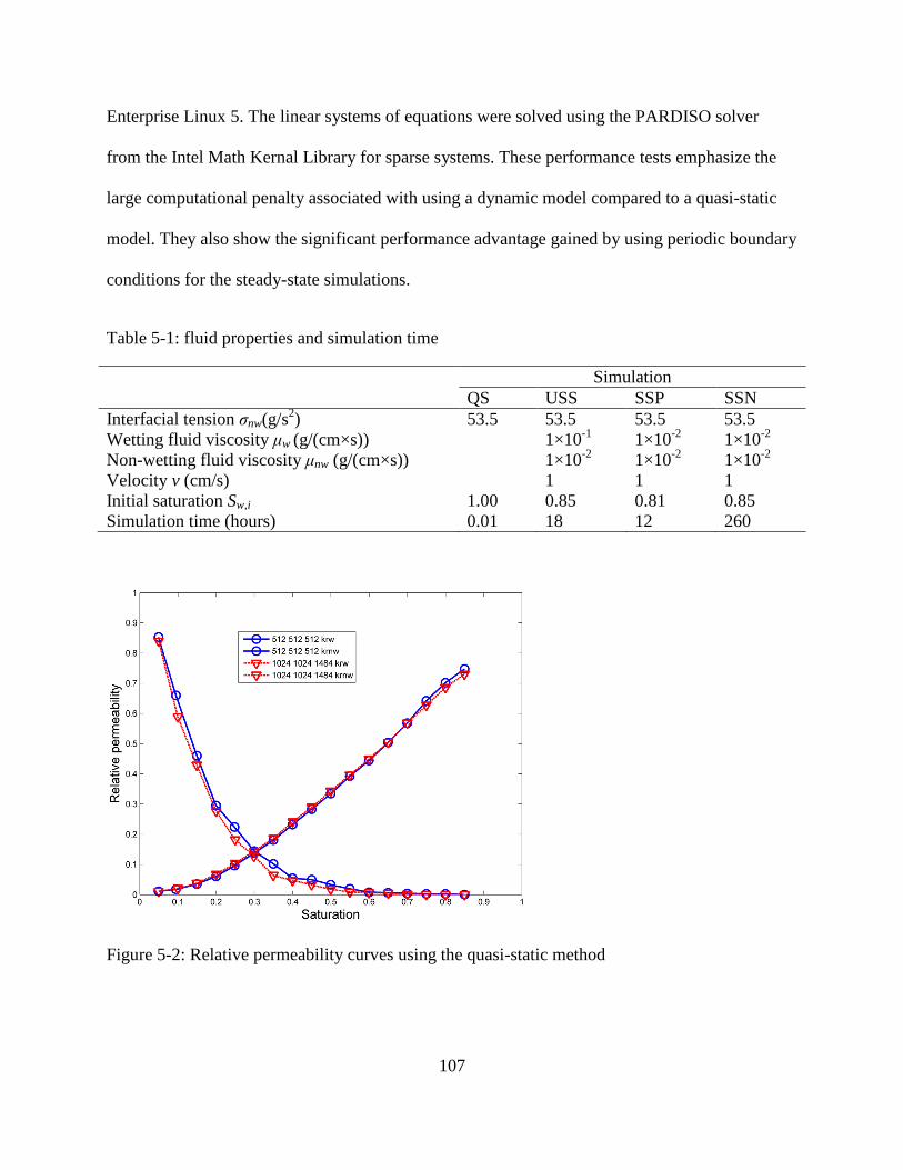
107

Enterprise Linux 5. The linear systems of equations were solved using the PARDISO solver

from the Intel Math Kernal Library for sparse systems. These performance tests emphasize the

large computational penalty associated with using a dynamic model compared to a quasi-static

model. They also show the significant performance advantage gained by using periodic boundary

conditions for the steady-state simulations.

Table 5-1: fluid properties and simulation time

Simulation

QS USS SSP SSN

Interfacial tension σnw(g/s2) 53.5 53.5 53.5 53.5

Wetting fluid viscosity μw (g/(cm×s)) 1×10-1

1×10-2

1×10-2

Non-wetting fluid viscosity μnw (g/(cm×s)) 1×10-2

1×10-2

1×10-2

Velocity v (cm/s) 1 1 1

Initial saturation Sw,i 1.00 0.85 0.81 0.85

Simulation time (hours) 0.01 18 12 260

Figure 5-2: Relative permeability curves using the quasi-static method

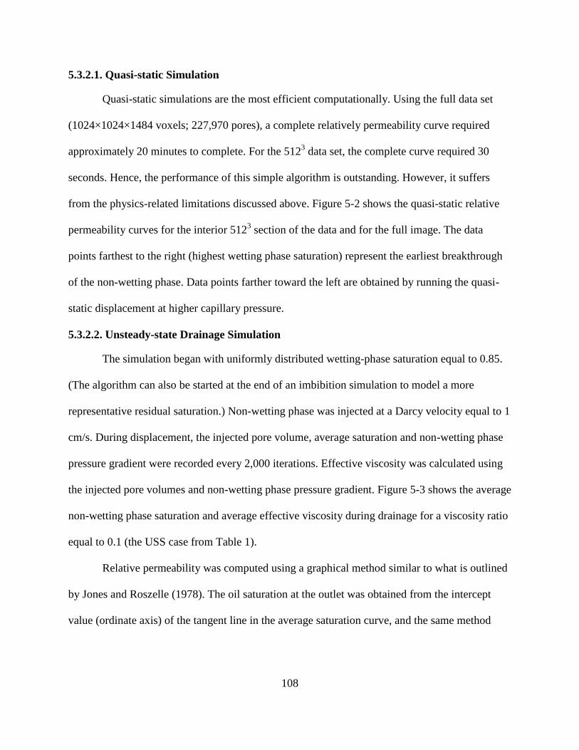
108

5.3.2.1. Quasi-static Simulation

Quasi-static simulations are the most efficient computationally. Using the full data set

(1024×1024×1484 voxels; 227,970 pores), a complete relatively permeability curve required

approximately 20 minutes to complete. For the 5123 data set, the complete curve required 30

seconds. Hence, the performance of this simple algorithm is outstanding. However, it suffers

from the physics-related limitations discussed above. Figure 5-2 shows the quasi-static relative

permeability curves for the interior 5123 section of the data and for the full image. The data

points farthest to the right (highest wetting phase saturation) represent the earliest breakthrough

of the non-wetting phase. Data points farther toward the left are obtained by running the quasi-

static displacement at higher capillary pressure.

5.3.2.2. Unsteady-state Drainage Simulation

The simulation began with uniformly distributed wetting-phase saturation equal to 0.85.

(The algorithm can also be started at the end of an imbibition simulation to model a more

representative residual saturation.) Non-wetting phase was injected at a Darcy velocity equal to 1

cm/s. During displacement, the injected pore volume, average saturation and non-wetting phase

pressure gradient were recorded every 2,000 iterations. Effective viscosity was calculated using

the injected pore volumes and non-wetting phase pressure gradient. Figure 5-3 shows the average

non-wetting phase saturation and average effective viscosity during drainage for a viscosity ratio

equal to 0.1 (the USS case from Table 1).

Relative permeability was computed using a graphical method similar to what is outlined

by Jones and Roszelle (1978). The oil saturation at the outlet was obtained from the intercept

value (ordinate axis) of the tangent line in the average saturation curve, and the same method

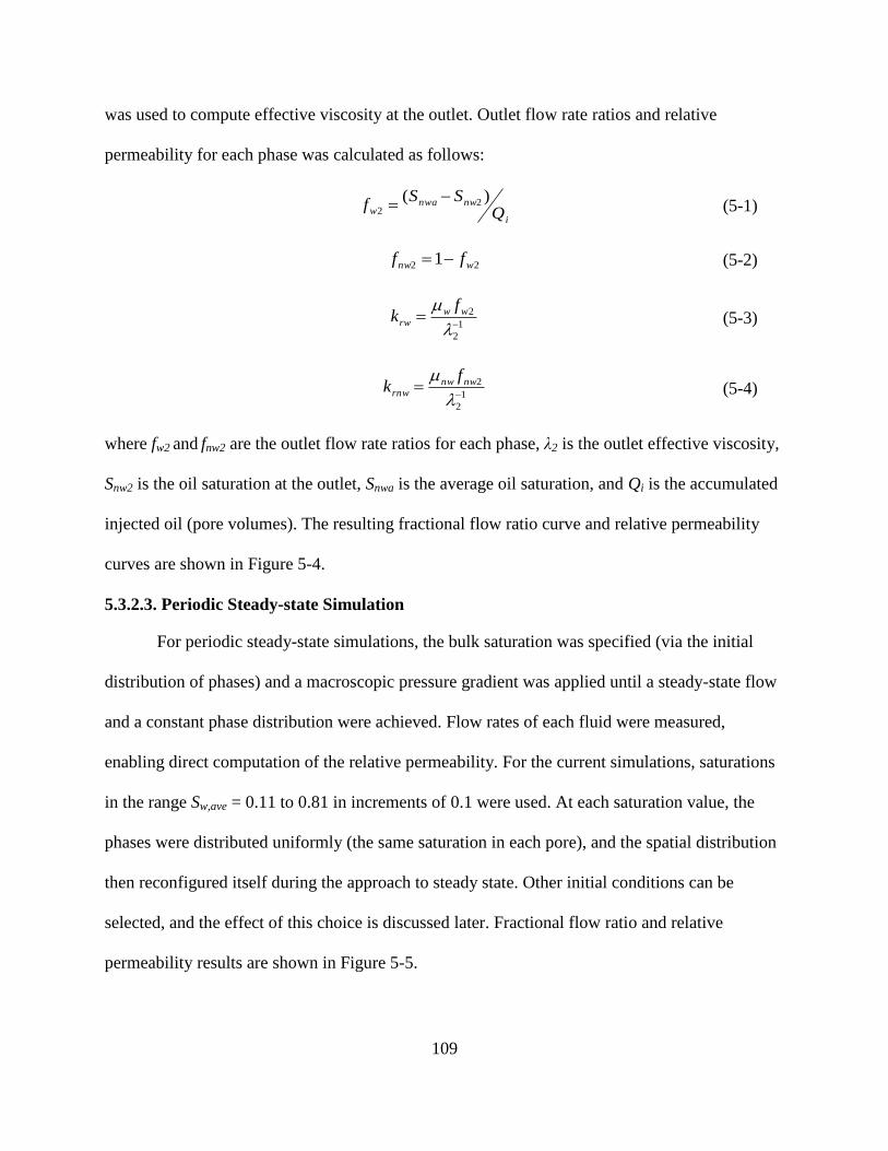
109

was used to compute effective viscosity at the outlet. Outlet flow rate ratios and relative

permeability for each phase was calculated as follows:

i

nwnwaw Q

SSf

)( 22

(5-1)

22 1 wnw ff (5-2)

1

2

2

wwrw

fk (5-3)

1

2

2

nwnwrnw

fk (5-4)

where fw2 and fnw2 are the outlet flow rate ratios for each phase, λ2 is the outlet effective viscosity,

Snw2 is the oil saturation at the outlet, Snwa is the average oil saturation, and Qi is the accumulated

injected oil (pore volumes). The resulting fractional flow ratio curve and relative permeability

curves are shown in Figure 5-4.

5.3.2.3. Periodic Steady-state Simulation

For periodic steady-state simulations, the bulk saturation was specified (via the initial

distribution of phases) and a macroscopic pressure gradient was applied until a steady-state flow

and a constant phase distribution were achieved. Flow rates of each fluid were measured,

enabling direct computation of the relative permeability. For the current simulations, saturations

in the range Sw,ave = 0.11 to 0.81 in increments of 0.1 were used. At each saturation value, the

phases were distributed uniformly (the same saturation in each pore), and the spatial distribution

then reconfigured itself during the approach to steady state. Other initial conditions can be

selected, and the effect of this choice is discussed later. Fractional flow ratio and relative

permeability results are shown in Figure 5-5.

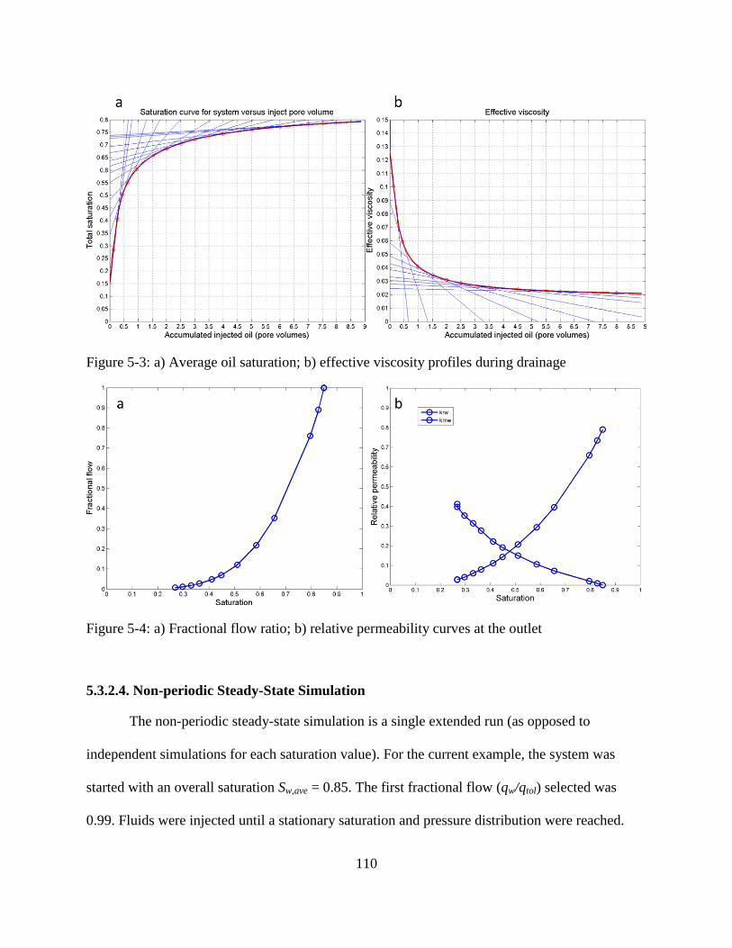
110

Figure 5-3: a) Average oil saturation; b) effective viscosity profiles during drainage

Figure 5-4: a) Fractional flow ratio; b) relative permeability curves at the outlet

5.3.2.4. Non-periodic Steady-State Simulation

The non-periodic steady-state simulation is a single extended run (as opposed to

independent simulations for each saturation value). For the current example, the system was

started with an overall saturation Sw,ave = 0.85. The first fractional flow (qw/qtol) selected was

0.99. Fluids were injected until a stationary saturation and pressure distribution were reached.

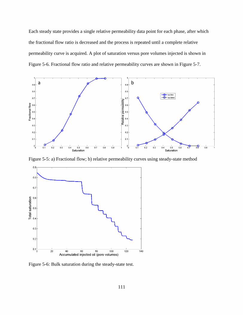
111

Each steady state provides a single relative permeability data point for each phase, after which

the fractional flow ratio is decreased and the process is repeated until a complete relative

permeability curve is acquired. A plot of saturation versus pore volumes injected is shown in

Figure 5-6. Fractional flow ratio and relative permeability curves are shown in Figure 5-7.

Figure 5-5: a) Fractional flow; b) relative permeability curves using steady-state method

Figure 5-6: Bulk saturation during the steady-state test.

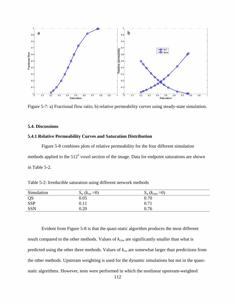
112

Figure 5-7: a) Fractional flow ratio; b) relative permeability curves using steady-state simulation.

5.4. Discussions

5.4.1 Relative Permeability Curves and Saturation Distribution

Figure 5-8 combines plots of relative permeability for the four different simulation

methods applied to the 5123 voxel section of the image. Data for endpoint saturations are shown

in Table 5-2.

Table 5-2: Irreducible saturation using different network methods

Simulation Sw (krw ≈0) Sw (krnw ≈0)

QS 0.05 0.70

SSP 0.11 0.71

SSN 0.20 0.76

Evident from Figure 5-8 is that the quasi-static algorithm produces the most different

result compared to the other methods. Values of krnw are significantly smaller than what is

predicted using the other three methods. Values of krw are somewhat larger than predictions from

the other methods. Upstream weighting is used for the dynamic simulations but not in the quasi-

static algorithms. However, tests were performed in which the nonlinear upstream-weighted

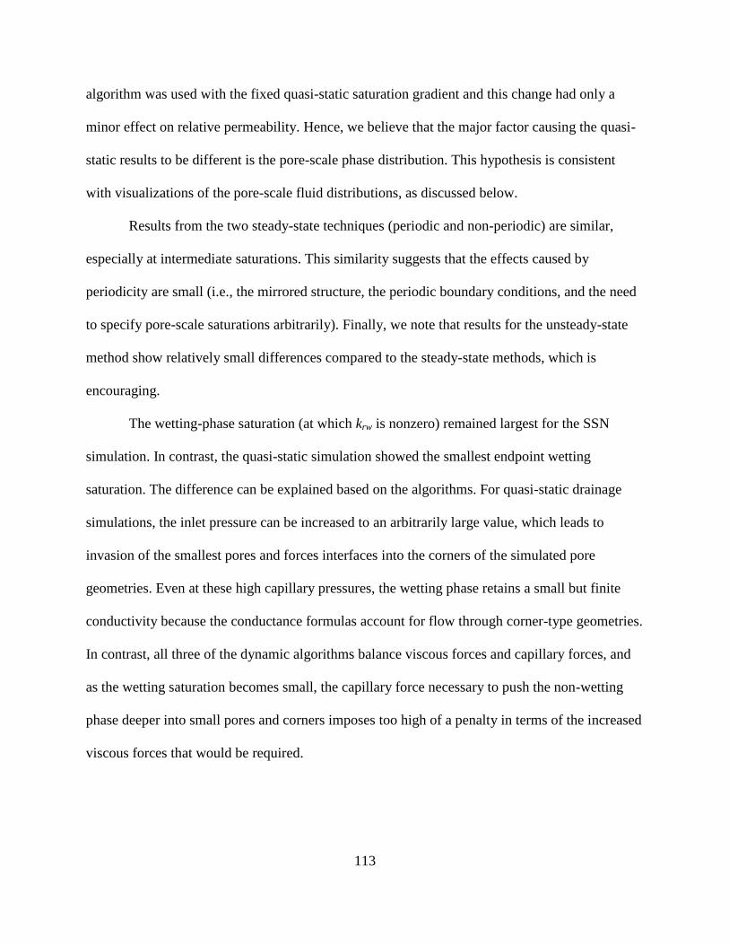
113

algorithm was used with the fixed quasi-static saturation gradient and this change had only a

minor effect on relative permeability. Hence, we believe that the major factor causing the quasi-

static results to be different is the pore-scale phase distribution. This hypothesis is consistent

with visualizations of the pore-scale fluid distributions, as discussed below.

Results from the two steady-state techniques (periodic and non-periodic) are similar,

especially at intermediate saturations. This similarity suggests that the effects caused by

periodicity are small (i.e., the mirrored structure, the periodic boundary conditions, and the need

to specify pore-scale saturations arbitrarily). Finally, we note that results for the unsteady-state

method show relatively small differences compared to the steady-state methods, which is

encouraging.

The wetting-phase saturation (at which krw is nonzero) remained largest for the SSN

simulation. In contrast, the quasi-static simulation showed the smallest endpoint wetting

saturation. The difference can be explained based on the algorithms. For quasi-static drainage

simulations, the inlet pressure can be increased to an arbitrarily large value, which leads to

invasion of the smallest pores and forces interfaces into the corners of the simulated pore

geometries. Even at these high capillary pressures, the wetting phase retains a small but finite

conductivity because the conductance formulas account for flow through corner-type geometries.

In contrast, all three of the dynamic algorithms balance viscous forces and capillary forces, and

as the wetting saturation becomes small, the capillary force necessary to push the non-wetting

phase deeper into small pores and corners imposes too high of a penalty in terms of the increased

viscous forces that would be required.

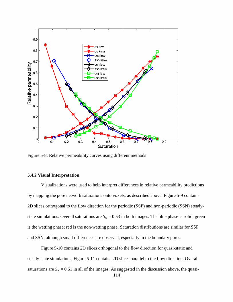
114

Figure 5-8: Relative permeability curves using different methods

5.4.2 Visual Interpretation

Visualizations were used to help interpret differences in relative permeability predictions

by mapping the pore network saturations onto voxels, as described above. Figure 5-9 contains

2D slices orthogonal to the flow direction for the periodic (SSP) and non-periodic (SSN) steady-

state simulations. Overall saturations are Sw = 0.53 in both images. The blue phase is solid; green

is the wetting phase; red is the non-wetting phase. Saturation distributions are similar for SSP

and SSN, although small differences are observed, especially in the boundary pores.

Figure 5-10 contains 2D slices orthogonal to the flow direction for quasi-static and

steady-state simulations. Figure 5-11 contains 2D slices parallel to the flow direction. Overall

saturations are Sw = 0.51 in all of the images. As suggested in the discussion above, the quasi-

115

static simulation shows a less uniform distribution of phases: pores contain either high non-

wetting phase saturation or remain completely saturated with wetting phase, but few pores

exhibit conditions in between. In contrast, the steady-state simulation shows a more uniform

distribution of fluids throughout all the pore space (which is a consequence of the competition

between capillary and viscous forces). This qualitative observation is consistent with the

relatively permeability results: the large number of pores that are fully saturated with wetting

phase for the QS simulation provides for a larger relative permeability to the wetting phase.

Similarly, the non-wetting phase pays a penalty in hydraulic resistance by not being able to use

many of the large pores in the QS simulation that are available for flow in the SSN simulation.


direction) for a) steady-state periodic simulation and b) steady-state non-periodic simulation at

Sw = 0.53

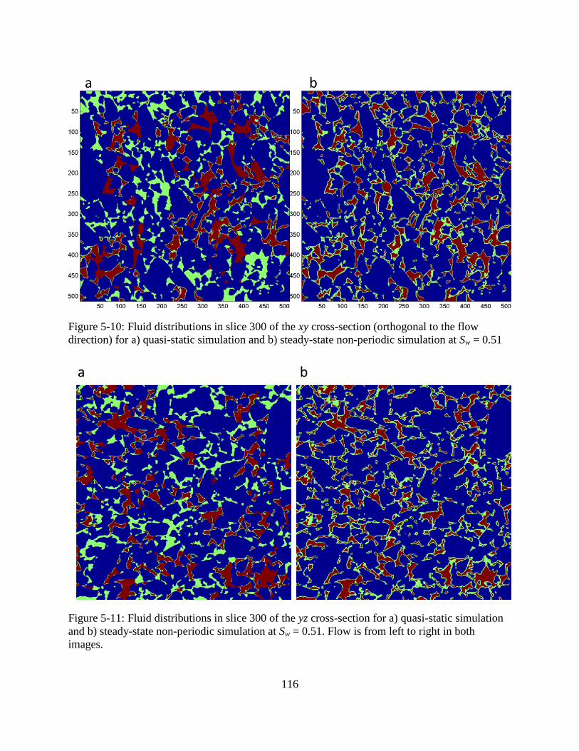
116


direction) for a) quasi-static simulation and b) steady-state non-periodic simulation at Sw = 0.51

Figure 5-11: Fluid distributions in slice 300 of the yz cross-section for a) quasi-static simulation

and b) steady-state non-periodic simulation at Sw = 0.51. Flow is from left to right in both

images.

117

Figure 5-12: Experimental versus simulated USS relative permeability

5.4.3 Comparison to Laboratory Data

Figure 5-12 shows data from high-rate (0.283 cm/s) and low-rate (0.0085 cm/s)

laboratory experiments using an unsteady-state technique. The viscosity ratio in the core flood

was μnw/μw = 1.6. Also shown are the USS data from the current simulations (performed at an

injection velocity of 1.0 cm/s and μnw/μw = 0.1). Although the simulated data do not agree well

with the current laboratory experiments, there are important differences between the two tests.

Particularly significant are the injection rates, the viscosity ratio, and the use of drainage in the

simulations versus imbibition in the core floods. As part of ongoing research, these values will

be matched in order to understand how sensitive the simulations are to these parameters and

whether the relative permeability curves shift in the correct direction as the simulation

parameters are changed. One other parameter worth noting is wettability, which can have a

118

dramatic impact on relative permeability but is difficult or impossible to quantify at a scale that

can be incorporated into digital images and pore-scale network models. Quantifying and using

wettability will be an important area of research in the future.

119

6. Dynamic Coupling of Pore-scale and Reservoir-scale Models

The concept of coupling pore- and continuum-scale models for subsurface flow has long

been viewed as beneficial, but implementation has been slow. This type of multiscale modeling

involves multiple considerations, from long-standing questions such as how one can effectively

characterize heterogeneous subsurface domains with a small number of samples as well as new

questions introduced by image-based modeling.

In this chapter, we present an algorithm for direct coupling of a dynamic pore-network

model for multiphase flow with a traditional continuum-scale simulator. The model is

implemented by embedding networks in selected gridblocks in the reservoir model, and tested

for variable-rate immiscible displacements under conditions in which relative permeability

depends on flowrate. Hurdles to implementing this type of modeling are also discussed.

6.1. Materials and Methods


Two types of porous materials were used in the current study: 1. unconsolidated sand

with grain sizes between 210 and 297 microns (Bhattad et al., 2011); 2. a consolidated sandstone

sample from a subsurface reservoir, described in more detail in Chapter 5. The samples were

imaged using x-ray microtomography (microCT) to obtain three-dimensional images. Although

larger images of both samples are available, internal sections of size 2003 voxel were used here

because of the large computational demands associated with running the steady-state algorithm,

especially with non-periodic conditions. These voxel dimensions correspond to 1,320.6 microns

on a side for the unconsolidated sand and 704 microns on a side for the sandstone. Networks

were generated from the microCT images using a network extraction algorithm described by

Thompson et al. (2008).

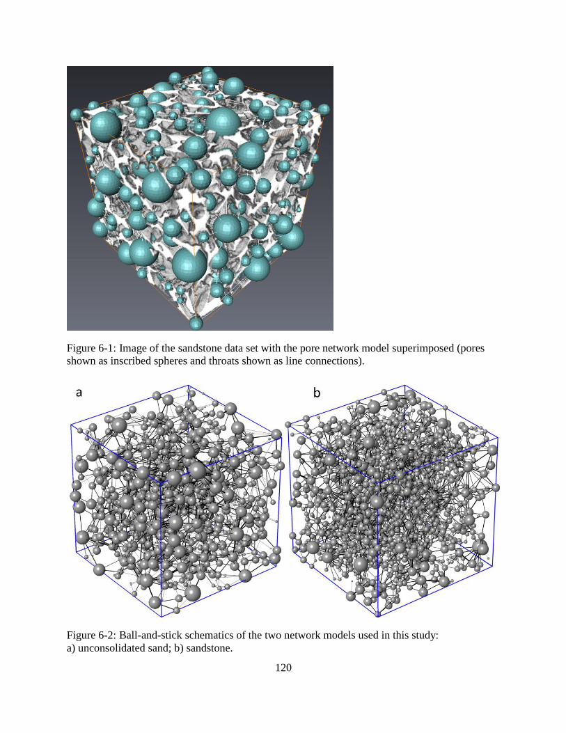
120

Figure 6-1: Image of the sandstone data set with the pore network model superimposed (pores

shown as inscribed spheres and throats shown as line connections).

Figure 6-2: Ball-and-stick schematics of the two network models used in this study:

a) unconsolidated sand; b) sandstone.

121

Figure 6-1 illustrates the network generation process by showing the 2003 voxel section

of the reservoir sandstone image with the corresponding network embedded in it. Figures 6-2a

and 6-2b are schematics of the two networks, which give a qualitative idea of differences in their

structures.

6.1.2. Dynamic Two-phase Network Model

Following Thompson (2002), two-phase flow is modeled by solving mass balance

equations for the two phases in each pore, which gives the following coupled non-linear

algebraic equations:

)()( ,,

,

,

1

, iwjw

j w

ijwrl

iw

l

iwi pp

ggSS

t

V

(6-1)

)()( ,,

,

,

1

, inwjnw

j nw

ijnwrl

inw

l

inwi pp

ggSS

t

V

where Vi is the volume of pore i and Si is the phase saturation (dimensionless volume fraction) in

pore i, gij is the throat conductance, μw and μnw are viscosity for each phase, and gr,w and gr,nw are

dimensionless relative throat conductance for each phase which account for the loss of

conductivity in the throat when a second immiscible phase is present. The dependent variables

are related by auxiliary equations such as saturation constricts local capillary pressure, throat

conductance and relative conductance.

1,, iwinw SS (6-2)


,....),( teffij lrfg (6-4)

)(/,/, trnwrwnwrwr Sfg (6-5)

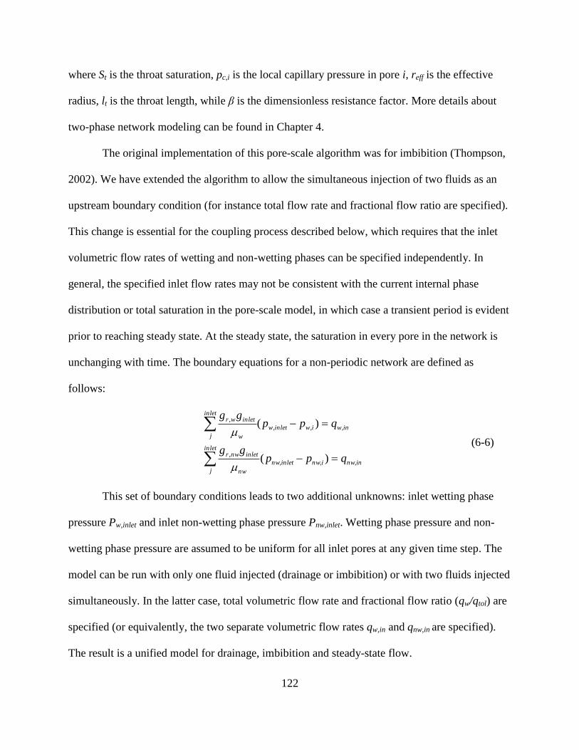
122

where St is the throat saturation, pc,i is the local capillary pressure in pore i, reff is the effective

radius, lt is the throat length, while β is the dimensionless resistance factor. More details about

two-phase network modeling can be found in Chapter 4.

The original implementation of this pore-scale algorithm was for imbibition (Thompson,

2002). We have extended the algorithm to allow the simultaneous injection of two fluids as an

upstream boundary condition (for instance total flow rate and fractional flow ratio are specified).

This change is essential for the coupling process described below, which requires that the inlet

volumetric flow rates of wetting and non-wetting phases can be specified independently. In

general, the specified inlet flow rates may not be consistent with the current internal phase

distribution or total saturation in the pore-scale model, in which case a transient period is evident

prior to reaching steady state. At the steady state, the saturation in every pore in the network is

unchanging with time. The boundary equations for a non-periodic network are defined as

follows:

innwinwinletnw

inlet

j nw

inletnwr

inwiwinletw

inlet

j w

inletwr

qppgg

qppgg

,,,

,

,,,

,

)(

)(

(6-6)

This set of boundary conditions leads to two additional unknowns: inlet wetting phase

pressure Pw,inlet and inlet non-wetting phase pressure Pnw,inlet. Wetting phase pressure and non-

wetting phase pressure are assumed to be uniform for all inlet pores at any given time step. The

model can be run with only one fluid injected (drainage or imbibition) or with two fluids injected

simultaneously. In the latter case, total volumetric flow rate and fractional flow ratio (qw/qtol) are

specified (or equivalently, the two separate volumetric flow rates qw,in and qnw,in are specified).

The result is a unified model for drainage, imbibition and steady-state flow.

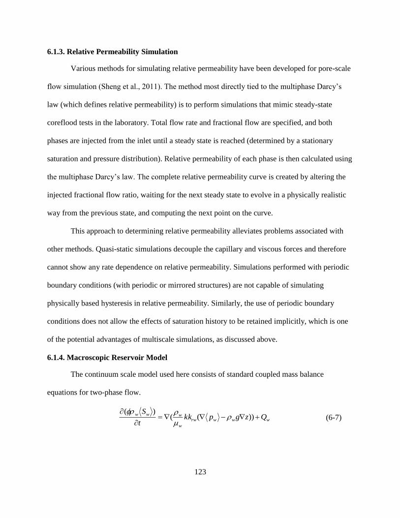
123

6.1.3. Relative Permeability Simulation

Various methods for simulating relative permeability have been developed for pore-scale

flow simulation (Sheng et al., 2011). The method most directly tied to the multiphase Darcy’s

law (which defines relative permeability) is to perform simulations that mimic steady-state

coreflood tests in the laboratory. Total flow rate and fractional flow are specified, and both

phases are injected from the inlet until a steady state is reached (determined by a stationary

saturation and pressure distribution). Relative permeability of each phase is then calculated using

the multiphase Darcy’s law. The complete relative permeability curve is created by altering the

injected fractional flow ratio, waiting for the next steady state to evolve in a physically realistic

way from the previous state, and computing the next point on the curve.

This approach to determining relative permeability alleviates problems associated with

other methods. Quasi-static simulations decouple the capillary and viscous forces and therefore

cannot show any rate dependence on relative permeability. Simulations performed with periodic

boundary conditions (with periodic or mirrored structures) are not capable of simulating

physically based hysteresis in relative permeability. Similarly, the use of periodic boundary

conditions does not allow the effects of saturation history to be retained implicitly, which is one

of the potential advantages of multiscale simulations, as discussed above.

6.1.4. Macroscopic Reservoir Model

The continuum scale model used here consists of standard coupled mass balance

equations for two-phase flow.

wwwrw

w

wwwQzgpkk

t

S

))((

)(

(6-7)

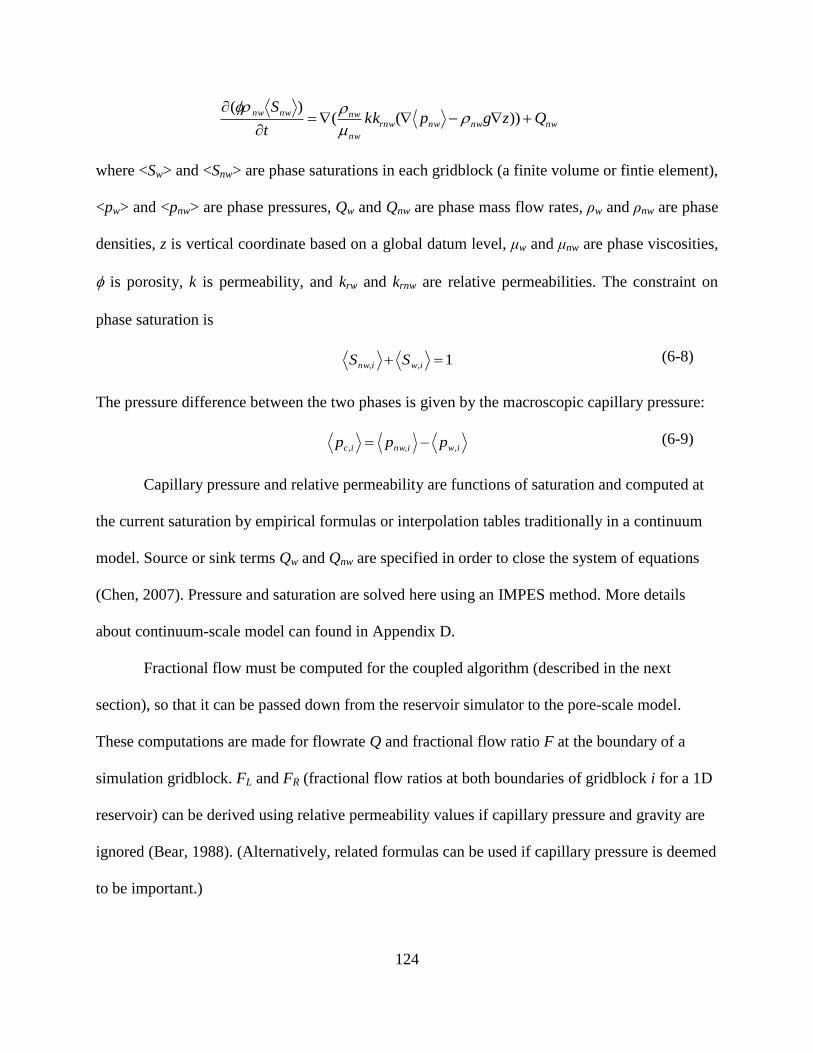
124

nwnwnwrnw

nw

nwnwnwQzgpkk

t

S

))((

)(

where <Sw> and <Snw> are phase saturations in each gridblock (a finite volume or fintie element),

<pw> and <pnw> are phase pressures, Qw and Qnw are phase mass flow rates, ρw and ρnw are phase

densities, z is vertical coordinate based on a global datum level, μw and μnw are phase viscosities,

is porosity, k is permeability, and krw and krnw are relative permeabilities. The constraint on

phase saturation is

1,, iwinw SS (6-8)

The pressure difference between the two phases is given by the macroscopic capillary pressure:


Capillary pressure and relative permeability are functions of saturation and computed at

the current saturation by empirical formulas or interpolation tables traditionally in a continuum

model. Source or sink terms Qw and Qnw are specified in order to close the system of equations

(Chen, 2007). Pressure and saturation are solved here using an IMPES method. More details

about continuum-scale model can found in Appendix D.

Fractional flow must be computed for the coupled algorithm (described in the next

section), so that it can be passed down from the reservoir simulator to the pore-scale model.

These computations are made for flowrate Q and fractional flow ratio F at the boundary of a

simulation gridblock. FL and FR (fractional flow ratios at both boundaries of gridblock i for a 1D

reservoir) can be derived using relative permeability values if capillary pressure and gravity are

ignored (Bear, 1988). (Alternatively, related formulas can be used if capillary pressure is deemed

to be important.)

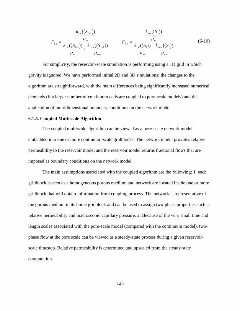
125

nw

irnw

w

irw

w

irw

iLSkSk

Sk

F

)()(

)(

11

1

,

nw

irnw

w

irw

w

irw

iRSkSk

Sk

F

)()(

)(

,

(6-10)

For simplicity, the reservoir-scale simulation is performing using a 1D grid in which

gravity is ignored. We have performed initial 2D and 3D simulations; the changes to the

algorithm are straightforward, with the main differences being significantly increased numerical

demands (if a larger number of continuum cells are coupled to pore-scale models) and the

application of multidimensional boundary conditions on the network model.

6.1.5. Coupled Multiscale Algorithm

The coupled multiscale algorithm can be viewed as a pore-scale network model

embedded into one or more continuum-scale gridblocks. The network model provides relative

permeability to the reservoir model and the reservoir model returns fractional flows that are

imposed as boundary conditions on the network model.

The main assumptions associated with the coupled algorithm are the following: 1. each

gridblock is seen as a homogeneous porous medium and network are located inside one or more

gridblock that will obtain information from coupling process. The network is representative of

the porous medium in its home gridblock and can be used to assign two-phase properties such as

relative permeability and macroscopic capillary pressure. 2. Because of the very small time and

length scales associated with the pore-scale model (compared with the continuum model), two-

phase flow at the pore scale can be viewed as a steady-state process during a given reservoir-

scale timestep. Relative permeability is determined and upscaled from the steady-state

computation.

126

Flow through two- or three-dimensional networks is approximated by applying pressure

on only two opposing faces (corresponding to the alignment with the reservoir model). This

assumption can be relaxed in 2D and 3D models with minor modifications; we have successfully

tested the 2D and 3D implementations for single-phase flow and believe the same approach can

be extended to multi-phase flow. Phase flowrates qnet for network models are calculated by

downscaling upstream flowrates Qgrid at the host gridblock boundary. The value for fractional

flow ratio imposed on the network model Fnet is calculated by linear interpolation between

fractional flows at both boundaries of the gridblock. For a network model placed in the center of

a gridblock, this would be

)(5.0 ,, iRiLnet FFF (6-11)

Network models are embedded into at least one continuum-scale gridblock. We assume

that initial conditions in the reservoir are known, and further assume that the initial pore-scale

saturation is known. In practice, the initial pore-scale phase distribution would come from either

the end of a separate simulation (for instance at the end of a Non-Aqueous Phase Liquid (NAPL)

spill simulation but prior to a remediation simulation, or at the end of primary oil production but

prior to water flooding) or inferred from a known condition (such as equilibrium water saturation

in a Vadose zone). Given the initial conditions at both the reservoir and pore scale, two-phase

properties such as relative permeability are determined. For each continuum-scale iteration, the

reservoir model provides fractional flows that are imposed as boundary conditions on the pore

network models. The network models are then run in order to update pore-scale saturation

distributions, and they return “real-time” relative permeability to their host gridblocks. Pore-

scale saturation and pressure distributions are stored locally for each coupled gridblock. The

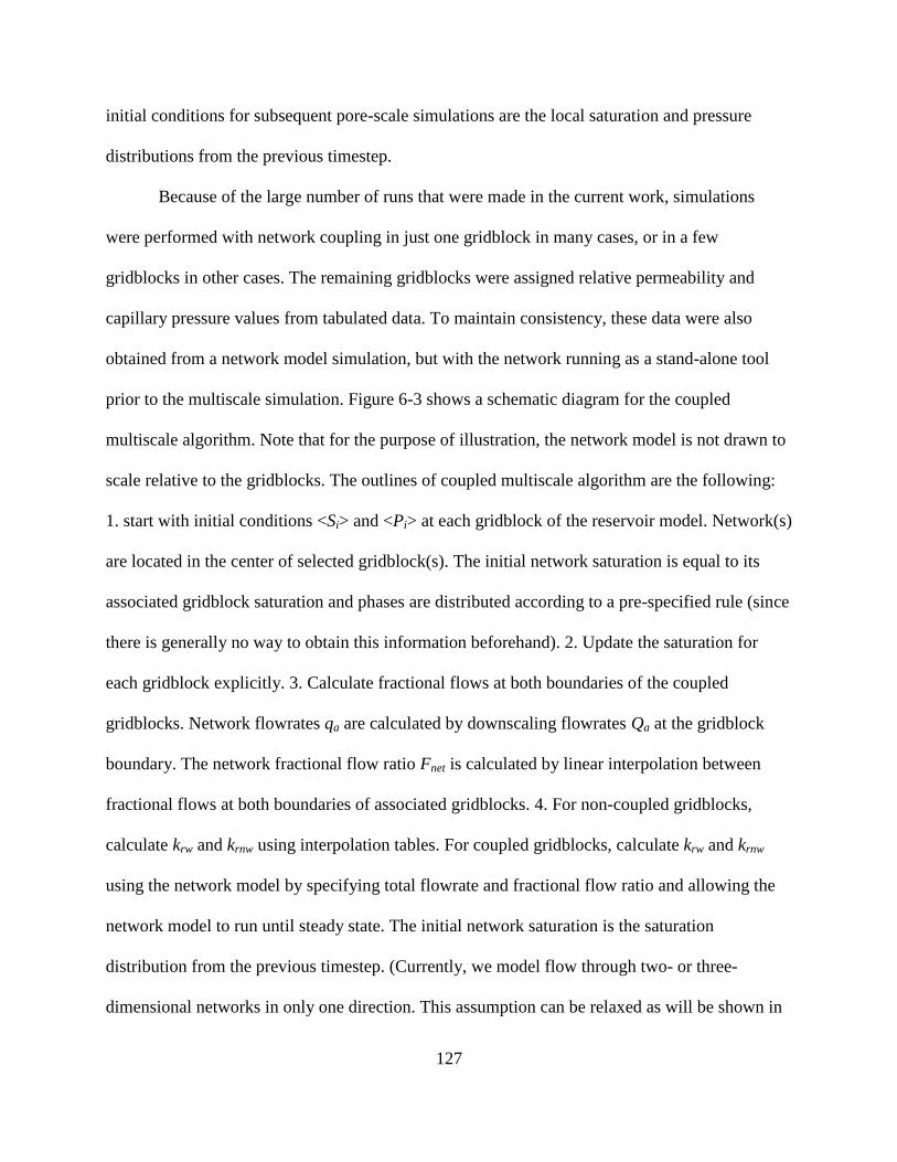
127

initial conditions for subsequent pore-scale simulations are the local saturation and pressure

distributions from the previous timestep.

Because of the large number of runs that were made in the current work, simulations

were performed with network coupling in just one gridblock in many cases, or in a few

gridblocks in other cases. The remaining gridblocks were assigned relative permeability and

capillary pressure values from tabulated data. To maintain consistency, these data were also

obtained from a network model simulation, but with the network running as a stand-alone tool

prior to the multiscale simulation. Figure 6-3 shows a schematic diagram for the coupled

multiscale algorithm. Note that for the purpose of illustration, the network model is not drawn to

scale relative to the gridblocks. The outlines of coupled multiscale algorithm are the following:

1. start with initial conditions <Si> and <Pi> at each gridblock of the reservoir model. Network(s)

are located in the center of selected gridblock(s). The initial network saturation is equal to its

associated gridblock saturation and phases are distributed according to a pre-specified rule (since

there is generally no way to obtain this information beforehand). 2. Update the saturation for

each gridblock explicitly. 3. Calculate fractional flows at both boundaries of the coupled

gridblocks. Network flowrates qa are calculated by downscaling flowrates Qa at the gridblock

boundary. The network fractional flow ratio Fnet is calculated by linear interpolation between

fractional flows at both boundaries of associated gridblocks. 4. For non-coupled gridblocks,

calculate krw and krnw using interpolation tables. For coupled gridblocks, calculate krw and krnw

using the network model by specifying total flowrate and fractional flow ratio and allowing the

network model to run until steady state. The initial network saturation is the saturation

distribution from the previous timestep. (Currently, we model flow through two- or three-

dimensional networks in only one direction. This assumption can be relaxed as will be shown in

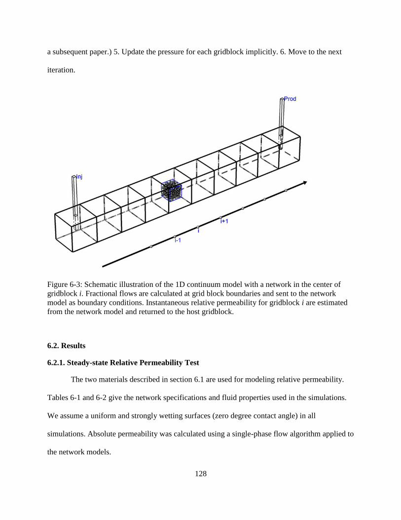
128

a subsequent paper.) 5. Update the pressure for each gridblock implicitly. 6. Move to the next

iteration.

Figure 6-3: Schematic illustration of the 1D continuum model with a network in the center of

gridblock i. Fractional flows are calculated at grid block boundaries and sent to the network

model as boundary conditions. Instantaneous relative permeability for gridblock i are estimated

from the network model and returned to the host gridblock.

6.2. Results

6.2.1. Steady-state Relative Permeability Test

The two materials described in section 6.1 are used for modeling relative permeability.

Tables 6-1 and 6-2 give the network specifications and fluid properties used in the simulations.

We assume a uniform and strongly wetting surfaces (zero degree contact angle) in all

simulations. Absolute permeability was calculated using a single-phase flow algorithm applied to

the network models.

129

Table 6-1: Network specifications

Number of

pores

Number of

throats

Dimension

(m)

Pore radius×106

(m)

Permeability×1012

(m2)

Sandstone 1,532 7,540 0.000704 [4.25~38.7] 2.90

Sand 882 4,862 0.00132 [7.97~89.7] 8.82

Table 6-2: Fluid parameters

Symbol Value Unit

Contact angle θ 0.0 degree

Interfacial tension σnw 0.0535 kg/s2

Wetting phase viscosity μw 0.00042 kg/(m×s)

Non-wetting phase viscosity μnw 0.0155 kg/(m×s)

Figure 6-4: Plots from the steady-state relative permeability test on the sandstone sample: a)

phase saturation versus pore-volumes injected; each plateau represents a steady-state relative

permeability data point; b) fractional flow ratio versus saturation; c) relative permeability curves.

For non-coupled gridblocks, relative permeability curves were calculated using steady-

state simulations with non-periodic conditions in a single extended run. Demonstration of the

steady-state test is performed using the sandstone network. The system was started with an

overall saturation Sw = 0.002. The first fractional flow (qw/qtol) selected was 0.005. Fluids were

injected until a stationary saturation distribution and pressure field were reached. Each steady-

state solution provided a single relative permeability data point for each phase, after which the

fractional flow ratio was increased and the process was repeated until a complete relative

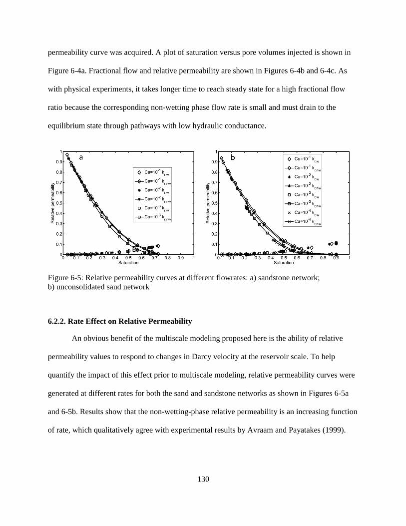
130

permeability curve was acquired. A plot of saturation versus pore volumes injected is shown in

Figure 6-4a. Fractional flow and relative permeability are shown in Figures 6-4b and 6-4c. As

with physical experiments, it takes longer time to reach steady state for a high fractional flow

ratio because the corresponding non-wetting phase flow rate is small and must drain to the

equilibrium state through pathways with low hydraulic conductance.

Figure 6-5: Relative permeability curves at different flowrates: a) sandstone network;

b) unconsolidated sand network

6.2.2. Rate Effect on Relative Permeability

An obvious benefit of the multiscale modeling proposed here is the ability of relative

permeability values to respond to changes in Darcy velocity at the reservoir scale. To help

quantify the impact of this effect prior to multiscale modeling, relative permeability curves were

generated at different rates for both the sand and sandstone networks as shown in Figures 6-5a

and 6-5b. Results show that the non-wetting-phase relative permeability is an increasing function

of rate, which qualitatively agree with experimental results by Avraam and Payatakes (1999).

131

6.2.3. Concurrent Model with a Constant Injection Rate

Demonstration of the concurrent multiscale model is performed using a 1D water

injection (more on the application is described below). The reservoir is divided into 100 blocks

along the flow direction. Injection occurs in the first block and fluids flows out of the last block.

Networks are embedded into selected gridblocks, and saturations in the networks and associated

gridblocks at these locations are used for most of the results below. The remaining gridblocks

obtain multiphase flow parameters from tabulated functions that are calculated a priori using

network simulations. Parameters used in the reservoir model are listed in Table 6-3.

Table 6-3: Simulation specification in the reservoir model

Symbol Value Unit

Nonwetting phase viscosity μnw 0.0155 kg/(m×s)

Wetting phase viscosity μw 0.00042 kg/(m×s)

Gridblock cross section area A 0.000929 m2

Gridblock length L 6.09600 m

Figure 6-6a shows network and gridblock saturation versus time in block #10. Saturations

in both the network and the gridblock start at <Sw> = 0.15 but after the first timestep the two

saturation values have already come to different values as fluid is reconfigured from the spatially

uniform saturation under an applied pressure gradient (see below). The more important

observation is that the network and gridblock saturations are not in good agreement. This

discrepancy presents a problem, but it is not entirely unexpected since there is no explicit

equation in the algorithm to force saturations in the network and associated gridblock to be

equal. It is tempting to add a saturation constraint to the algorithm to maintain equality.

However, we have avoided this approach because the constraint does not arise naturally from the

governing equations and because it would require either an explicit correction at the continuum

132

scale (which would conflict with the underlying conservation equation), or an ad-hoc re-

distribution of phases in the pore-scale model (which would in effect erase all implicit history

dependence).

Figure 6-6: a) Saturation comparison between the network and its associated gridblock for β = 8

(cylindrical throat shape). The sandstone network was embedded in gridblock 10. b) Comparison

of the network and reservoir fractional flow curves for β = 8. c) Saturation comparison between

the network and its associated gridblock β = 65.02 (for equilateral triangular throat shape). d)

Comparison of the network and reservoir fractional flow curves for β = 65.02.

Numerous tests were performed to track the divergent saturations, both at the outset of

the simulations and in other cases where the two saturation curves crossed, so were essentially

equal for a timestep, but then diverged again. These numerical tests showed that the problem can

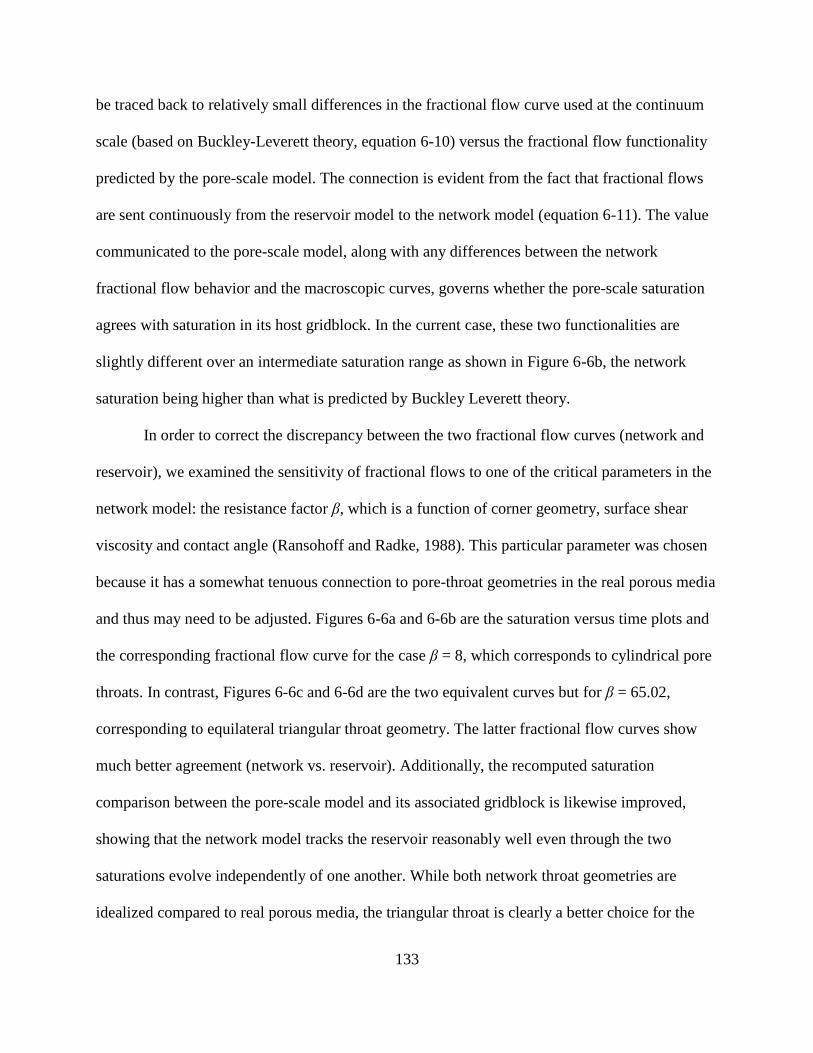
133

be traced back to relatively small differences in the fractional flow curve used at the continuum

scale (based on Buckley-Leverett theory, equation 6-10) versus the fractional flow functionality

predicted by the pore-scale model. The connection is evident from the fact that fractional flows

are sent continuously from the reservoir model to the network model (equation 6-11). The value

communicated to the pore-scale model, along with any differences between the network

fractional flow behavior and the macroscopic curves, governs whether the pore-scale saturation

agrees with saturation in its host gridblock. In the current case, these two functionalities are

slightly different over an intermediate saturation range as shown in Figure 6-6b, the network

saturation being higher than what is predicted by Buckley Leverett theory.

In order to correct the discrepancy between the two fractional flow curves (network and

reservoir), we examined the sensitivity of fractional flows to one of the critical parameters in the

network model: the resistance factor β, which is a function of corner geometry, surface shear

viscosity and contact angle (Ransohoff and Radke, 1988). This particular parameter was chosen

because it has a somewhat tenuous connection to pore-throat geometries in the real porous media

and thus may need to be adjusted. Figures 6-6a and 6-6b are the saturation versus time plots and

the corresponding fractional flow curve for the case β = 8, which corresponds to cylindrical pore

throats. In contrast, Figures 6-6c and 6-6d are the two equivalent curves but for β = 65.02,

corresponding to equilateral triangular throat geometry. The latter fractional flow curves show

much better agreement (network vs. reservoir). Additionally, the recomputed saturation

comparison between the pore-scale model and its associated gridblock is likewise improved,

showing that the network model tracks the reservoir reasonably well even through the two

saturations evolve independently of one another. While both network throat geometries are

idealized compared to real porous media, the triangular throat is clearly a better choice for the

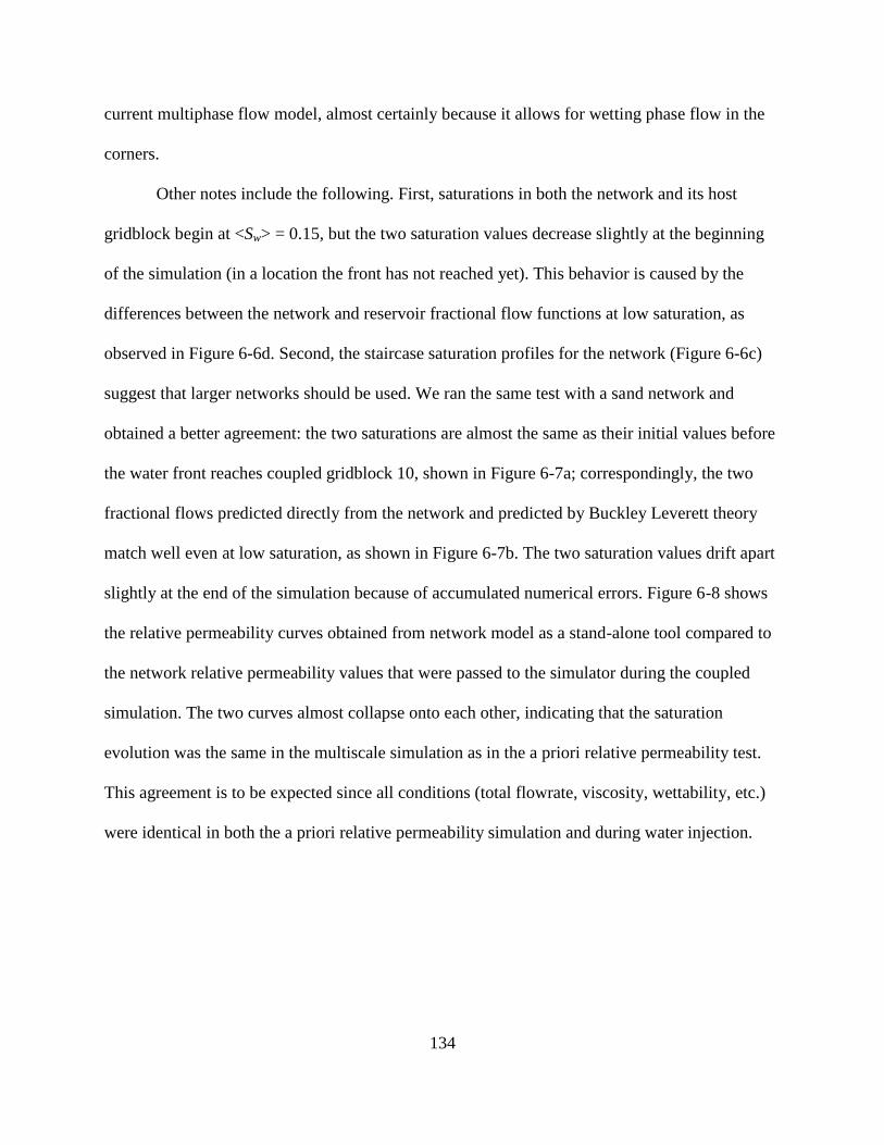
134

current multiphase flow model, almost certainly because it allows for wetting phase flow in the

corners.

Other notes include the following. First, saturations in both the network and its host

gridblock begin at <Sw> = 0.15, but the two saturation values decrease slightly at the beginning

of the simulation (in a location the front has not reached yet). This behavior is caused by the

differences between the network and reservoir fractional flow functions at low saturation, as

observed in Figure 6-6d. Second, the staircase saturation profiles for the network (Figure 6-6c)

suggest that larger networks should be used. We ran the same test with a sand network and

obtained a better agreement: the two saturations are almost the same as their initial values before

the water front reaches coupled gridblock 10, shown in Figure 6-7a; correspondingly, the two

fractional flows predicted directly from the network and predicted by Buckley Leverett theory

match well even at low saturation, as shown in Figure 6-7b. The two saturation values drift apart

slightly at the end of the simulation because of accumulated numerical errors. Figure 6-8 shows

the relative permeability curves obtained from network model as a stand-alone tool compared to

the network relative permeability values that were passed to the simulator during the coupled

simulation. The two curves almost collapse onto each other, indicating that the saturation

evolution was the same in the multiscale simulation as in the a priori relative permeability test.

This agreement is to be expected since all conditions (total flowrate, viscosity, wettability, etc.)

were identical in both the a priori relative permeability simulation and during water injection.

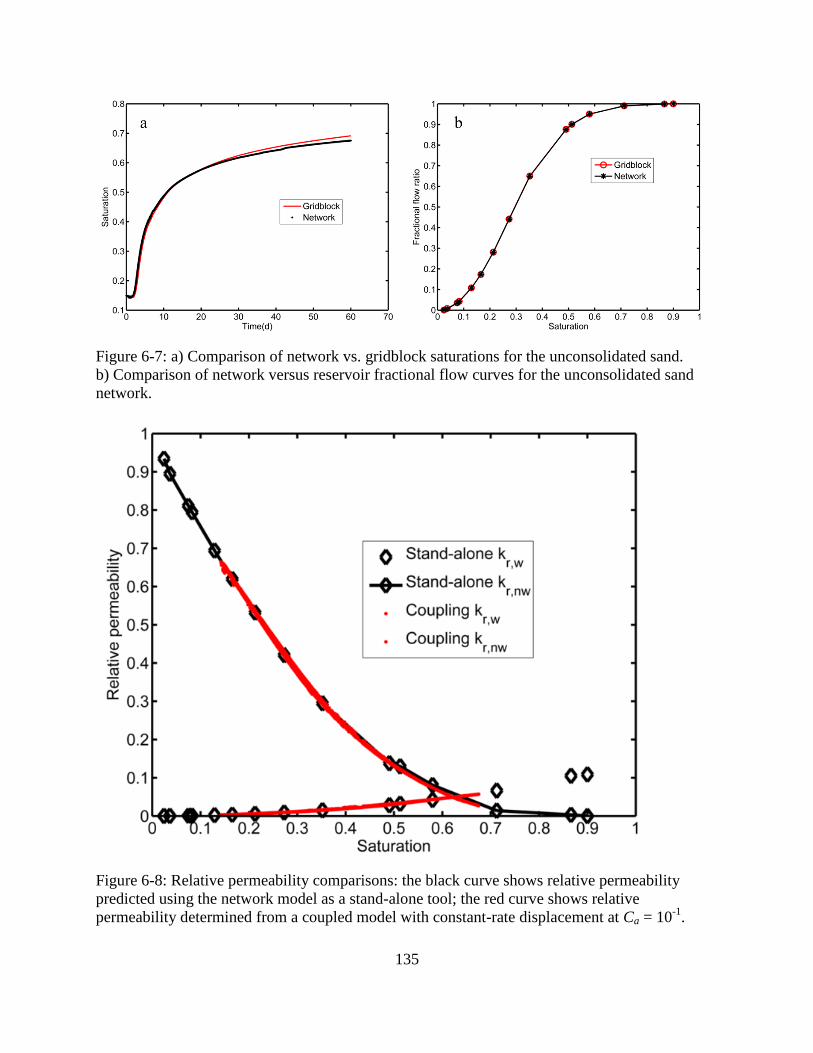
135

Figure 6-7: a) Comparison of network vs. gridblock saturations for the unconsolidated sand.

b) Comparison of network versus reservoir fractional flow curves for the unconsolidated sand

network.

Figure 6-8: Relative permeability comparisons: the black curve shows relative permeability

predicted using the network model as a stand-alone tool; the red curve shows relative

permeability determined from a coupled model with constant-rate displacement at Ca = 10-1

.

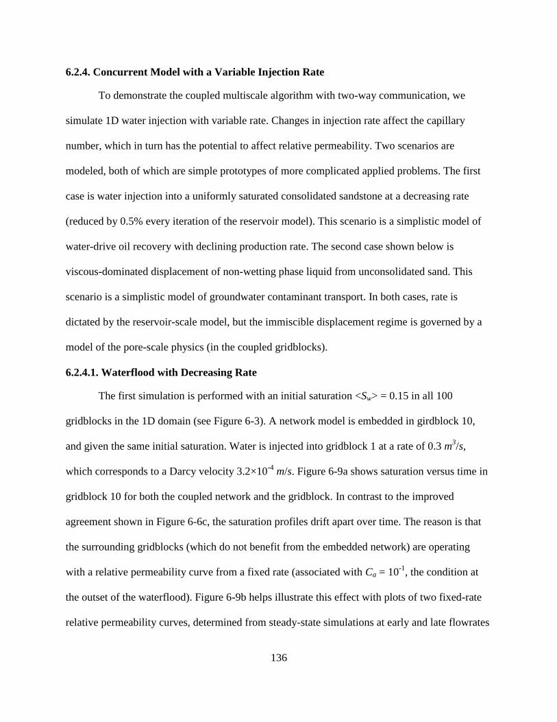
136

6.2.4. Concurrent Model with a Variable Injection Rate

To demonstrate the coupled multiscale algorithm with two-way communication, we

simulate 1D water injection with variable rate. Changes in injection rate affect the capillary

number, which in turn has the potential to affect relative permeability. Two scenarios are

modeled, both of which are simple prototypes of more complicated applied problems. The first

case is water injection into a uniformly saturated consolidated sandstone at a decreasing rate

(reduced by 0.5% every iteration of the reservoir model). This scenario is a simplistic model of

water-drive oil recovery with declining production rate. The second case shown below is

viscous-dominated displacement of non-wetting phase liquid from unconsolidated sand. This

scenario is a simplistic model of groundwater contaminant transport. In both cases, rate is

dictated by the reservoir-scale model, but the immiscible displacement regime is governed by a

model of the pore-scale physics (in the coupled gridblocks).

6.2.4.1. Waterflood with Decreasing Rate

The first simulation is performed with an initial saturation <Sw> = 0.15 in all 100

gridblocks in the 1D domain (see Figure 6-3). A network model is embedded in girdblock 10,

and given the same initial saturation. Water is injected into gridblock 1 at a rate of 0.3 m3/s,

which corresponds to a Darcy velocity 3.2×10-4

m/s. Figure 6-9a shows saturation versus time in

gridblock 10 for both the coupled network and the gridblock. In contrast to the improved

agreement shown in Figure 6-6c, the saturation profiles drift apart over time. The reason is that

the surrounding gridblocks (which do not benefit from the embedded network) are operating

with a relative permeability curve from a fixed rate (associated with Ca = 10-1

, the condition at

the outset of the waterflood). Figure 6-9b helps illustrate this effect with plots of two fixed-rate

relative permeability curves, determined from steady-state simulations at early and late flowrates

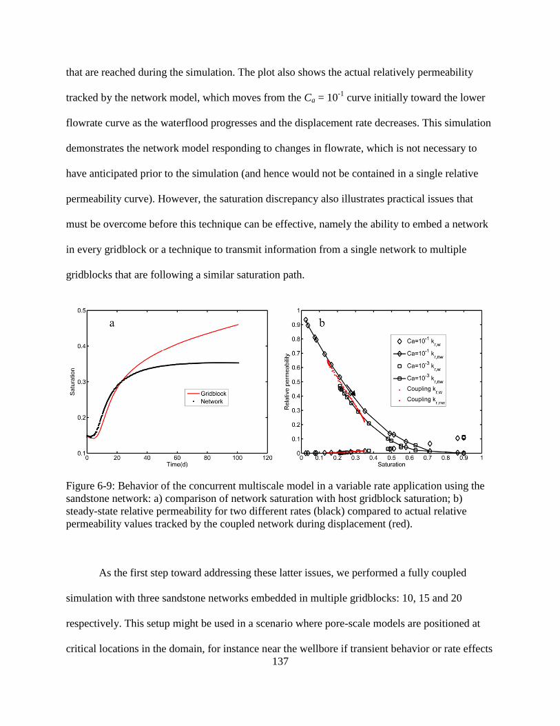
137

that are reached during the simulation. The plot also shows the actual relatively permeability

tracked by the network model, which moves from the Ca = 10-1

curve initially toward the lower

flowrate curve as the waterflood progresses and the displacement rate decreases. This simulation

demonstrates the network model responding to changes in flowrate, which is not necessary to

have anticipated prior to the simulation (and hence would not be contained in a single relative

permeability curve). However, the saturation discrepancy also illustrates practical issues that

must be overcome before this technique can be effective, namely the ability to embed a network

in every gridblock or a technique to transmit information from a single network to multiple

gridblocks that are following a similar saturation path.

Figure 6-9: Behavior of the concurrent multiscale model in a variable rate application using the

sandstone network: a) comparison of network saturation with host gridblock saturation; b)

steady-state relative permeability for two different rates (black) compared to actual relative

permeability values tracked by the coupled network during displacement (red).

As the first step toward addressing these latter issues, we performed a fully coupled

simulation with three sandstone networks embedded in multiple gridblocks: 10, 15 and 20

respectively. This setup might be used in a scenario where pore-scale models are positioned at

critical locations in the domain, for instance near the wellbore if transient behavior or rate effects

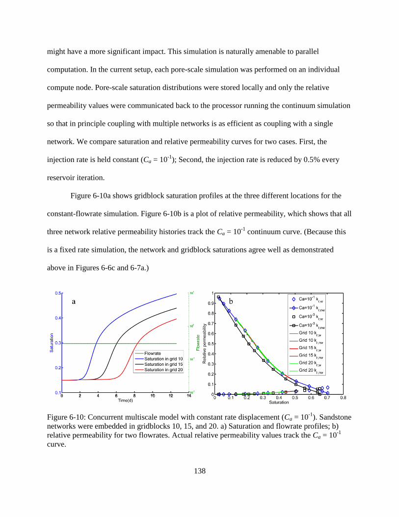
138

might have a more significant impact. This simulation is naturally amenable to parallel

computation. In the current setup, each pore-scale simulation was performed on an individual

compute node. Pore-scale saturation distributions were stored locally and only the relative

permeability values were communicated back to the processor running the continuum simulation

so that in principle coupling with multiple networks is as efficient as coupling with a single

network. We compare saturation and relative permeability curves for two cases. First, the

injection rate is held constant (Ca = 10-1

); Second, the injection rate is reduced by 0.5% every

reservoir iteration.

Figure 6-10a shows gridblock saturation profiles at the three different locations for the

constant-flowrate simulation. Figure 6-10b is a plot of relative permeability, which shows that all

three network relative permeability histories track the Ca = 10-1

continuum curve. (Because this

is a fixed rate simulation, the network and gridblock saturations agree well as demonstrated

above in Figures 6-6c and 6-7a.)

Figure 6-10: Concurrent multiscale model with constant rate displacement (Ca = 10-1

). Sandstone

networks were embedded in gridblocks 10, 15, and 20. a) Saturation and flowrate profiles; b)

relative permeability for two flowrates. Actual relative permeability values track the Ca = 10-1

curve.

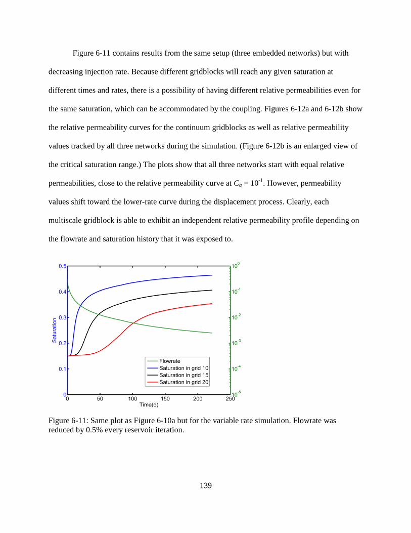
139

Figure 6-11 contains results from the same setup (three embedded networks) but with

decreasing injection rate. Because different gridblocks will reach any given saturation at

different times and rates, there is a possibility of having different relative permeabilities even for

the same saturation, which can be accommodated by the coupling. Figures 6-12a and 6-12b show

the relative permeability curves for the continuum gridblocks as well as relative permeability

values tracked by all three networks during the simulation. (Figure 6-12b is an enlarged view of

the critical saturation range.) The plots show that all three networks start with equal relative

permeabilities, close to the relative permeability curve at Ca = 10-1

. However, permeability

values shift toward the lower-rate curve during the displacement process. Clearly, each

multiscale gridblock is able to exhibit an independent relative permeability profile depending on

the flowrate and saturation history that it was exposed to.

Figure 6-11: Same plot as Figure 6-10a but for the variable rate simulation. Flowrate was

reduced by 0.5% every reservoir iteration.

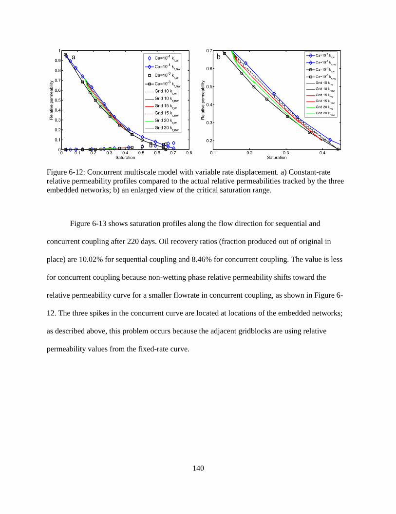
140

Figure 6-12: Concurrent multiscale model with variable rate displacement. a) Constant-rate

relative permeability profiles compared to the actual relative permeabilities tracked by the three

embedded networks; b) an enlarged view of the critical saturation range.

Figure 6-13 shows saturation profiles along the flow direction for sequential and

concurrent coupling after 220 days. Oil recovery ratios (fraction produced out of original in

place) are 10.02% for sequential coupling and 8.46% for concurrent coupling. The value is less

for concurrent coupling because non-wetting phase relative permeability shifts toward the

relative permeability curve for a smaller flowrate in concurrent coupling, as shown in Figure 6-

12. The three spikes in the concurrent curve are located at locations of the embedded networks;

as described above, this problem occurs because the adjacent gridblocks are using relative

permeability values from the fixed-rate curve.

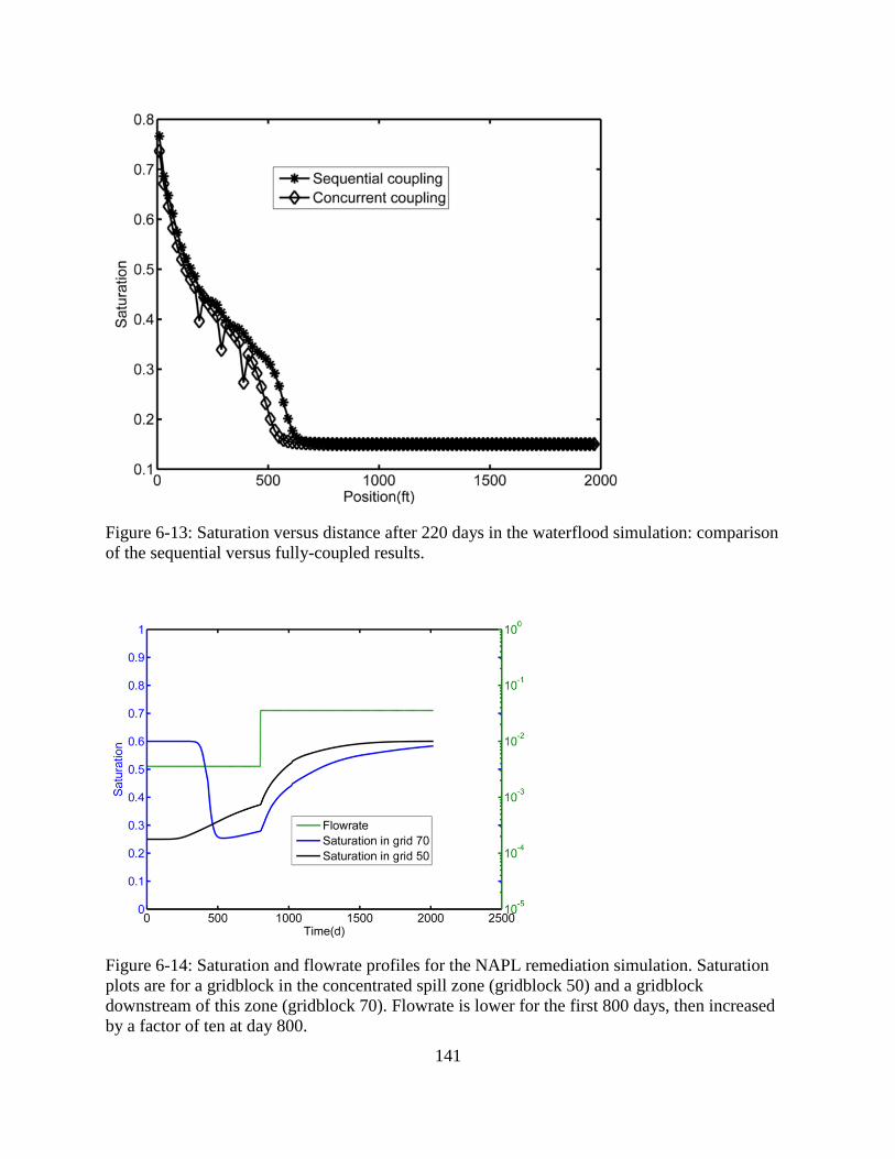
141

Figure 6-13: Saturation versus distance after 220 days in the waterflood simulation: comparison

of the sequential versus fully-coupled results.

Figure 6-14: Saturation and flowrate profiles for the NAPL remediation simulation. Saturation

plots are for a gridblock in the concentrated spill zone (gridblock 50) and a gridblock

downstream of this zone (gridblock 70). Flowrate is lower for the first 800 days, then increased

by a factor of ten at day 800.

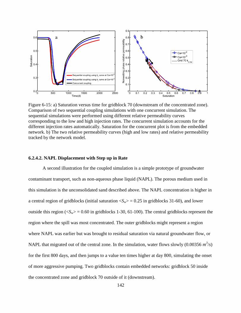
142

Figure 6-15: a) Saturation versus time for gridblock 70 (downstream of the concentrated zone).

Comparison of two sequential coupling simulations with one concurrent simulation. The

sequential simulations were performed using different relative permeability curves

corresponding to the low and high injection rates. The concurrent simulation accounts for the

different injection rates automatically. Saturation for the concurrent plot is from the embedded

network. b) The two relative permeability curves (high and low rates) and relative permeability

tracked by the network model.

6.2.4.2. NAPL Displacement with Step up in Rate

A second illustration for the coupled simulation is a simple prototype of groundwater

contaminant transport, such as non-aqueous phase liquid (NAPL). The porous medium used in

this simulation is the unconsolidated sand described above. The NAPL concentration is higher in

a central region of gridblocks (initial saturation <Sw> = 0.25 in gridblocks 31-60), and lower

outside this region (<Sw> = 0.60 in gridblocks 1-30, 61-100). The central gridblocks represent the

region where the spill was most concentrated. The outer gridblocks might represent a region

where NAPL was earlier but was brought to residual saturation via natural groundwater flow, or

NAPL that migrated out of the central zone. In the simulation, water flows slowly (0.00356 m3/s)

for the first 800 days, and then jumps to a value ten times higher at day 800, simulating the onset

of more aggressive pumping. Two gridblocks contain embedded networks: gridblock 50 inside

the concentrated zone and gridblock 70 outside of it (downstream).

143

Figure 6-14 shows continuum-scale saturation profiles in gridblocks 50 and 70 for

concurrent coupling. It also shows the flowrate, which increases tenfold on day 800. Gridblock

50 shows little change for the first 200 days, as the water injection front has not yet reached this

location. Cleanup is steady but slow between 200 and 800 days. The rate of cleanup increases

dramatically at day 800. The change is associated largely with the increased displacement rate

but the coupling means that it will also capture any improvement in displacement efficiency that

would occur because of the shift to a higher capillary number regime for immiscible

displacement. Gridblock 70 is downstream of the concentrated NAPL zone. Hence, water

saturation decreases dramatically as the NAPL is pushed through this region. It then begins to

clean up with similar behavior as the upstream gridblock.

Again addressing the impact of the full coupling, note Figure 6-15a, which provides a

comparison of two pure continuum scale simulations: one with a relative permeability curve

associated with the higher displacement rate, one with the lower rate. A significant difference

exists between the two simulations. In principle, one could of course switch between relative

permeability curves at the flow transition point. However, this approach will work only if one

has relative permeability curves for all operating conditions a priori (and can parameterize the

relative permeability curves in terms of factors that may vary in the simulation). Figure 6-15a

also shows saturation in the network model that is embedded in gridblock 70. It tracks the low-

flowrate simulation more closely at early times and the high flowrate simulation more closely at

later times, as might be expected. The unsmooth behavior in the range 500-800 days is caused by

numerical instabilities in the pore-scale model, which are most pronounced in a dynamic

multiphase model when operating at low wetting-phase saturations and low capillary number

conditions. For completeness, we include Figure 6-15b, which tracks relative permeability values

144

in gridblock 70 during the displacement. These plots illustrate the jump from one curve to the

other at day 800.

Figure 6-16 shows saturation profiles along the flow direction for sequential (low-

flowrate simulation) and concurrent coupling after 1,000 days. As with the waterflood example,

the sequential versus concurrent coupling lead to different amounts of NAPL recovered: 1.95%

for sequential coupling and 3.68% for concurrent coupling at day 1,000. The value is higher for

the concurrent simulation because the non-wetting phase relative permeabilities shift to higher

values once the flowrate is increased.

Figure 6-16: Saturation versus distance along the injection direction at day 1,000 for the NAPL

example. Comparison of sequential versus concurrent coupling.

145

7. Conclusions and Recommendations

This work focused on pore-to-continuum multiscale coupling, and a number of numerical

issues that enable the technology. The ultimate goal for this area of research is to quantify

physical processes at different scales. This work incorporated a set of novel algorithms into a

single workflow. It is described in four stand-alone chapters (Chapters 3-6).

Chapter 3 investigated the impact of pore-scale morphology and hydraulic conductance

formula on single-phase flow in porous media. Chapter 4 presented a new dynamic network

model that allows two phases to be injected simultaneously even with non-periodic boundary

conditions. Although flow simulations in Chapters 3 and 4 were conducted at the pore scale, the

results could provide information on macroscopic properties at a larger scale. The research in

Chapter 5 focused on relative permeability prediction using different numerical approaches.

Chapter 6 described a novel concurrent coupling algorithm which couples the dynamic two-

phase network models with a continuum model. The multiscale model was able to respond to

varied reservoir conditions such as injection rate or local saturation history as no previous model

has been able to.

In this final Chapter, the goal is to summarize the results from each part of the research

and provide recommendations for the future research regarding pore-to-continuum multiscale

coupling.

7.1. Conclusions

7.1.1. Single-phase Network Model

Network modeling provides an efficient first-principles approach to determine

macroscopic properties in porous media. The predicted network permeability values were

compared with direct simulation results (LBM and FEM) using computer-generated porous

146

materials. It has been shown that the predicted permeability is sensitive to two important

parameters in network modeling: the merging criterion during network generation and the

formula used for hydraulic conductance calculations. The results subsequently suggest that

permeability matching alone is not adequate for network validation.

A more rigorous option for network validation is to compare the pore-scale flow rate

distribution from the network versus that from direct simulations. The sensitivity of this flow

distribution to the merging criterion and conductance method has been studied comprehensively.

For all tested runs, the optimum choices are conductance method 260 (Thompson and Fogler,

1997) combined with the DT network generation algorithm. Method 260 computes throat

conductance using BEM, and accounts for the actual throat shape as well as the converging

diverging feature along the flow paths. A more efficient pore-scale model has been developed

using a fitted conductance formula based on BEM conductance, which results in an improvement

in both flow prediction accuracy and simulation speed.

A network approach has been developed for the first time to determine the full

permeability tensor and principal flow directions. Tests show that the predicted principal flow

directions are in good agreement with the known anisotropy of a prototype sphere packing. An

appealing feature of this approach is that the predicted principal flow direction is fairly

insensitive to the network parameters such as conductance method. This work is encouraging

because it shows that network models can augment traditional core analysis in certain

applications.

7.1.2. Two-phase Network Model

A unified two-phase dynamic network model (which couples viscous force and capillary

force directly) has been used to simulate two-phase flow under both transient and steady-state

147

conditions successfully. The model can be run with a single phase injected or two phases

simultaneously injected. This capability is particularly useful to describe a broader range of flow

conditions in a reservoir, such as concurrent flow or counter-current flow. The dynamic two-

phase model includes pore-level physics such as snap off, cooperative filling and film flow. To

produce computationally feasible algorithms, simplified auxiliary functions were introduced to

describe the aforementioned pore-level physics.

The unified network model provides detailed pressure and saturation fields within the

porous media. This information can then be used to provide macroscopic relative permeability.

Both periodic and non-periodic boundary conditions have been used to simulate steady-state

flow. Periodic steady-state simulations fail to track saturation history. In contrast, steady-state

simulations using a non-periodic network account for behaviors associated with hysteresis and

saturation history. Steady-state simulation using a non-periodic domain mimics the experimental

setup for a steady-state relative permeability test, and allows one to use the multiphase Darcy’s

law directly for computing relative permeability. A drainage and imbibition cycle was simulated

using a non-periodic sandstone network. Although all the simulations were conducted at strongly

wetting conditions, the relative permeability results clearly exhibited a hysteresis effect. It was

also noted that hysteresis is mainly controlled by the pore-scale displacement sequence.

The sensitivity of relative permeability to parameters such as capillary number and

saturation history has been investigated. While those dependencies have been observed in

experiments, the two-phase network model provides a fast first-principles numerical approach to

interpret those phenomena, which is currently the weak link for macroscopic simulations. The

advantages of this approach are not limited to sensitivity analysis. The ability to simulate both

148

transient and steady-state conditions allows pore-scale models to evolve naturally based on

conditions provided from reservoir simulations.


Network modeling is a promising method to simulate relative permeability using image-

based modeling. Numerous approaches and/or algorithms exist for performing these simulations,

but little information is available regarding differences between algorithms or appropriateness of

any one algorithm for certain conditions. Hence, decisions are generally made ad hoc or

according to what algorithms are available. We present simulated relative permeability for a

reservoir sandstone that was imaged using microCT. Four algorithms are used for the

simulations, and the results are compared. Conclusions and observations include the following.

1. The quasi-static algorithm, which is the most widely used algorithm because of its

simplicity, has the best computational performance by a significant margin. Complete relative

permeability curves were obtained in seconds or minutes depending on the size of the network.

However, the quasi-static relative permeability results are the most different compared to the

other algorithms used, and this approach is questionable in terms of whether physics are captured

in a reasonable way.

2. The unsteady-state and steady-state simulations gave surprisingly similar results given

the significant differences in the simulation and data interpretation techniques.

3. Periodic and non-periodic steady-state results are nearly identical. This similarity is

encouraging in one sense because the periodic simulations are more computationally efficient.

However, the need to specify an initial condition for periodic simulations (or the assumption that

the results will be independent of the initial condition specified) is problematic in light of the

known hysteretic behavior of relative permeability.

149

4. Pore-scale phase distributions were estimated from the network saturations and

mapped onto the original voxel images. These images, while qualitative, can be used to help

interpret the different results seen in one algorithm versus another and will prove useful for

validation against more rigorous simulations. Saturation visualizations reveal stark differences

between quasi-static and dynamic results. The dynamic models produce more uniform phase

distributions within the pore space as compared to the percolation structures obtained via quasi-

static displacement. This difference enables the wetting phase to occupy more conductive

portions of the void space in the quasi-static simulations, which in turn shifts the wetting phase

relative permeability to higher values and the non-wetting-phase relative permeability to lower

values, as compared to the dynamic simulations.

7.1.4. Multiscale Coupling

The potential benefits of integrating first-principles pore-scale models into macroscopic

simulators have been understood for many years. However, the algorithmic challenges and

computational demands associated with this type of multiscale modeling have made it slow to be

put into practice, even at the research scale. This study represents the first time that multiphase

pore-scale models have been embedded into gridblocks in a reservoir simulation so that they

operate concurrently: the network provides just-in-time relative permeability values to the host

gridblock in the reservoir simulator so that the relative permeability value reflects current

properties and dynamics as well as saturation history.

The development that allowed this concurrent multiscale algorithm to be implemented is

the algorithm discussed in section 7.1.2, which provides the ability to perform pore-scale

simulation of the simultaneous injection of two fluids under transient or steady-state conditions

for non-periodic domains. Typical boundary conditions for these pore-scale simulations are the

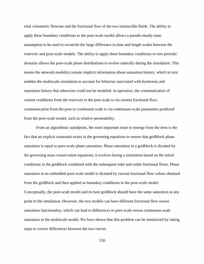
150

total volumetric flowrate and the fractional flow of the two immiscible fluids. The ability to

apply these boundary conditions to the pore-scale model allows a pseudo-steady-state

assumption to be used to reconcile the large difference in time and length scales between the

reservoir and pore-scale models. The ability to apply these boundary conditions to non-periodic

domains allows the pore-scale phase distributions to evolve naturally during the simulation. This

means the network model(s) contain implicit information about saturation history, which in turn

enables the multiscale simulation to account for behavior associated with hysteresis and

saturation history that otherwise could not be modeled. In operation, the communication of

current conditions from the reservoir to the pore scale is via current fractional flow;

communication from the pore to continuum scale is via continuum-scale parameters predicted

from the pore-scale model, such as relative permeability.

From an algorithmic standpoint, the most important issue to emerge from the tests is the

fact that no explicit constraint exists in the governing equations to ensure that gridblock phase

saturation is equal to pore-scale phase saturation. Phase saturation in a gridblock is dictated by

the governing mass conservation equations; it evolves during a simulation based on the initial

conditions in the gridblock combined with the subsequent inlet and outlet fractional flows. Phase

saturation in an embedded pore-scale model is dictated by current fractional flow values obtained

from the gridblock and then applied as boundary conditions in the pore-scale model.

Conceptually, the pore-scale model and its host gridblock should have the same saturation at any

point in the simulation. However, the two models can have different fractional flow versus

saturation functionality, which can lead to differences in pore-scale versus continuum-scale

saturation in the multiscale model. We have shown that this problem can be minimized by taking

steps to correct differences between the two curves.

151

7.2. Recommendations

The recommendations of possible future work are presented here in the aspects of the

work for each chapter (Chapters 3-6).

7.2.1. Single-phase Network Model

Network flow distributions have been compared with direct simulation results (LBM and

FEM) for computer-generated unconsolidated sphere packings. However, pore structures in a

consolidated rock are significantly different with computer-generated unconsolidated packings.

Consequently, the network algorithms that performed well for unconsolidated packings may not

predict fluid flow as well for consolidated materials (Sheng et al., 2011). In the future, a more

comprehensive benchmark comparison should be conducted for different types of rock samples.

Velocity distributions can be obtained using either in-house FEM algorithm, commercial CFD

software such as COMSOL, or LBM simulations. In these tests, the network is mapped

rigorously from the same materials as the direct simulations are performed on. Velocities from

direct simulations can be interpolated and compared with average network velocity in the same

pore throats. In complex scenarios such as reaction flow or inertial flow, information should be

exchanged in both directions since throat conductance is considered as nonlinear functions of the

macroscopic properties (Chu et al., 2012). The network models provide macroscopic properties

such as pressure or flow rate; FEM models provide real-time throat conductance.

Single-phase network models are fast and powerful tools for large microCT data (billions

of voxels) because they use a reduced data set (103-10

5 pores). Even so, the size of image-based

modeling is limited by the size of the original image (Idowu, 2009). In the future, research on

computer-generated porous structure needs to be expanded. Multiple methods (such as simulated

annealing techniques) could be tested to generate multiscale porous media.

152

Possible correlation between electrical anisotropy and permeability anisotropy has

received particular attention (Anderson et al., 1994). Similarity was seen in 1D network

simulations for electrical resistivity (Appendix B) and permeability. In Chapter 3, a network

approach has been developed to determine the full permeability tensor and principal flow

directions. This approach should be extended to calculate the full resistivity tensor in the future,

which may provide clues to a fundamental understanding of the relationship between resistivity

and permeability.

7.2.2. Two-phase Network Model

A more general approach to obtaining the local capillary pressure curve should be

developed to account for the variety of pore geometry and invasion patterns. Thompson (2002)

used a test sphere to probe a series of spatial locations inside a pore and calculate capillary

pressure based on inscribed radius of the test sphere. Similar research should be conducted on

other porous materials in the framework of image-based network modeling. Depending on

whether saturation is increasing or decreasing, the local capillary pressure is different because of

hysteretic effects (Patzek, 2001). Therefore, a multivariable tabulation for the local capillary

pressure function should be created when hysteretic effects become important.

The impact of relative conductance equations on two-phase network simulations should

be investigated. Two-phase flow has been simulated using commercial CFD software in a regular

porous structure, as shown in Figure 7-1. This type of approach can be used to compare relative

conductance formulas, and they can be fitted using a hybrid network-CFD model.

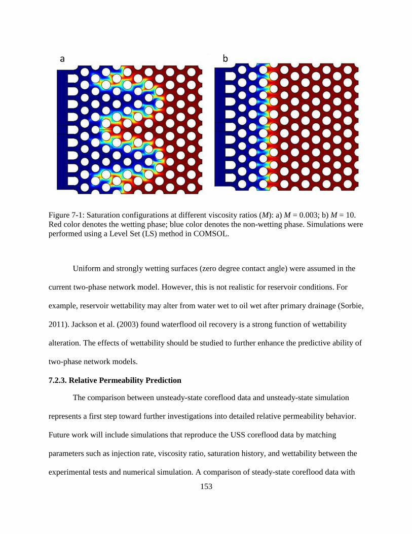
153

Figure 7-1: Saturation configurations at different viscosity ratios (M): a) M = 0.003; b) M = 10.

Red color denotes the wetting phase; blue color denotes the non-wetting phase. Simulations were

performed using a Level Set (LS) method in COMSOL.

Uniform and strongly wetting surfaces (zero degree contact angle) were assumed in the

current two-phase network model. However, this is not realistic for reservoir conditions. For

example, reservoir wettability may alter from water wet to oil wet after primary drainage (Sorbie,

2011). Jackson et al. (2003) found waterflood oil recovery is a strong function of wettability

alteration. The effects of wettability should be studied to further enhance the predictive ability of

two-phase network models.


The comparison between unsteady-state coreflood data and unsteady-state simulation

represents a first step toward further investigations into detailed relative permeability behavior.

Future work will include simulations that reproduce the USS coreflood data by matching

parameters such as injection rate, viscosity ratio, saturation history, and wettability between the

experimental tests and numerical simulation. A comparison of steady-state coreflood data with

154

steady-state simulations should also be conducted. Comparison of macroscopic relative

permeability curves will help to understand what level of confidence in a simulator can be

gained.

Some questions will likely remain open until technology allows the imaging of pore-scale

phase distributions in conjunction with relative permeability tests. The results from transient

study of phase distributions using microCT imaging should be used to validate and fine tune the

two-phase network model in the future.

7.2.4. Multiscale Coupling

The concurrent multiscale approach has been demonstrated using simulations of rate

dependent behavior. However, the advantages of this approach are not limited to this application.

The ability for a reservoir-scale model to obtain continuum parameters directly from a first-

principles model enables it to respond to any number of phenomena that are not captured by

simple empirical relationships or tabulated parameters. Examples include permeability loss due

to deep bed filtration, flow instabilities causes by chemical injection, or changes to the porous

media itself due to subsidence, fracturing, or acidizing. A more subtle advantage of the

concurrent multiscale modeling shown here is the ability for the pore-scale model to serve as an

implicit record of the saturation history. Hence, parameters that exhibit hysteresis or history

dependence respond to the underlying physics that cause these effects.

The performance of multiscale simulations should be improved for practicality. First,

efforts should be made to optimize computational performance of the steady-state dynamic

multiphase flow simulations, which are the most computationally demanding of the many

network modeling algorithms that we have implemented (especially at low wetting-phase

saturations or flowrates). Other network algorithms such as dynamic displacement or periodic

155

steady-state simulations may be considered for multiscale coupling, which would reduce the

computational load on the pore-scale side. Additionally, we have run selected tests in which

communication with the embedded networks occurs less often (i.e., not at every reservoir

timestep). Preliminary results show that speed can be increased considerably while maintaining

good accuracy.

156

References Cited

Aarnes, J. E., V. Kippe, et al. (2007). Modelling of multiscale structures in flow simulations for

petroleum reservoirs geometric modelling, numerical simulation, and optimization. G.

Hasle, K.-A. Lie and E. Quak, Springer Berlin Heidelberg: 307-360.

Aker, E., K. Jørgen Måiøy, et al. (1998). "A Two-Dimensional Network Simulator for Two-

Phase Flow in Porous Media." Transport in Porous Media 32(2): 163-186.

Al-Gharbi, M. S. and M. J. Blunt (2005). "Dynamic network modeling of two-phase drainage in

porous media." Physical Review E 71(1).

Al-Kharusi, A. S. and M. J. Blunt (2008). "Multiphase flow predictions from carbonate pore

space images using extracted network models." Water Resour. Res. 44(6): W06S01.

Al-Raoush, R., K. Thompson, et al. (2003). "Comparison of network generation techniques for

unconsolidated porous media." Soil Science Society of America Journal 67(6): 1687-

1700.

Anderson, B., K. Helbig, et al. (1994). "Oilfield anisotropy: Its origins and electrical

characteristics." Oilfield Review 6(4): 48-56.

Arns, J.-Y., C. H. Arns, et al. (2003). "Relative permeability from tomographic images; effect of

correlated heterogeneity." Journal of Petroleum Science and Engineering 39(3-4): 247-

259.

Avraam, D. G. and A. C. Payatakes (1999). "Flow mechanisms, relative permeabilities, and

coupling effects in steady-state two-phase flow through porous media. the case of strong

wettability." Industrial & Engineering Chemistry Research 38(3): 778-786.

Bakke, S. and P. E. Øren (1997). "3-D pore-scale modelling of sandstones and flow simulations

in the pore networks." SPE Journal 2(2): 136-149.

Balhoff, M., S. Thomas, et al. (2008). "Mortar coupling and upscaling of pore-scale models."

Computational Geosciences 12(1): 15-27.

Balhoff, M. T., K. E. Thompson, et al. (2007). "Coupling pore-scale networks to continuum-

scale models of porous media." Computers & Geosciences 33(3): 393-410.

Bardon C; Longeron, D. G. (1980). "Influence of very low interfacial tensions on relative

permeability." Old SPE Journal 20(5): 391-401.

Bear, J. (1988). Dynamics of fluids in porous media, Dover publications.

157

Benson, S. M. and D. R. Cole (2008). "CO2 sequestration in deep sedimentary formations."

Elements 4(5): 325-331.

Bhattad, P., C. S. Willson, et al. (2011). "Effect of Network Structure on Characterization and

Flow Modeling Using X-ray Micro-Tomography Images of Granular and Fibrous Porous

Media." Transport in Porous Media 90(2): 363-391.

Biswal, B., P. E. Øren, et al. (2009). "Modeling of multiscale porous media." Image Analysis and

Stereology 28: 23-34.

Blower, J. (2001). "A three-dimensional network model of permeability in vesicular material."

Computers & Geosciences 27(1): 115-119.

Blunt, M., M. J. King, et al. (1992). "Simulation and Theory of 2-Phase Flow in Porous-Media."

Physical Review A 46(12): 7680-7699.

Blunt, M. and P. King (1991). "Relative Permeabilities from 2-Dimensional and 3-Dimensional

Pore-Scale Network Modeling." Transport in Porous Media 6(4): 407-433.

Blunt, M. J. (1997). "Effects of Heterogeneity and Wetting on Relative Permeability Using Pore

Level Modeling " SPE Journal 2(1): 70-87.

Blunt, M. J. (2001). "Flow in porous media—pore-network models and multiphase flow."

Current opinion in colloid & interface science 6(3): 197-207.

Blunt, M. J., M. D. Jackson, et al. (2002). "Detailed physics, predictive capabilities and

macroscopic consequences for pore-network models of multiphase flow." Advances in

Water Resources 25(8-12): 1069-1089.

Blunt, M. J. and H. Scher (1995). "Pore-Level Modeling of Wetting." Physical Review E 52(6):

6387-6403.

Boek, E. (2010). Pore Scale Simulation of Flow in Porous Media Using Lattice-Boltzmann

Computer Simulations. SPE Annual Technical Conference and Exhibition.

Bryant, S. and M. Blunt (1992). "Prediction of Relative Permeability in Simple Porous-Media."

Physical Review A 46(4): 2004-2011.

Bryant, S. and N. Pallatt (1996). "Predicting formation factor and resistivity index in simple

sandstones." Journal of Petroleum Science and Engineering 15(2): 169-179.

Bryant, S. L., P. R. King, et al. (1993). "Network model evaluation of permeability and spatial

correlation in a real random sphere packing." Transport in Porous Media 11(1): 53-70.

Bryant, S. L., D. W. Mellor, et al. (1993). "Physically Representative Network Models of

Transport in Porous-Media." AIChE Journal 39(3): 387-396.

158

Celia, M. A., H. Rajaram, et al. (1993). "A multi-scale computational model for multiphase flow

in porous media." Advances in Water Resources 16(1): 81-92.

Chen, C., A. I. Packman, et al. (2010). "A multi-scale investigation of interfacial transport, pore

fluid flow, and fine particle deposition in a sediment bed." Water Resour. Res. 46(11):

W11560.

Chen, Z. (2007). Reservoir simulation: mathematical techniques in oil recovery. Philadelphia,

PA, SIAM.

Chu, J., B. Engquist, et al. (2012a). A multi-scale method coupling network and continuum

models in porous media II – single and two phase flow.

Chu, J., B. Engquist, et al. (2012b). "A multiscale method coupling network and continuum

models in porous media I: steady-state single phase flow." Multiscale Modeling &

Simulation 10(2): 515-549.

Constantinides, G. N. and A. C. Payatakes (1996). "Network simulation of steady-state two-

phase flow in consolidated porous media." AIChE Journal 42(2): 369-382.

Dadvar, M. and M. Sahimi (2003). "Pore network model of deactivation of immobilized glucose

isomerase in packed-bed reactors. Part III: Multiscale modelling." Chemical engineering

science 58(22): 4935-4951.

Dahle, H. K. and M. A. Celia (1999). "A dynamic network model for two‐phase immiscible

flow." Computational Geosciences 3(1): 1-22.

Dias, M. M. and A. C. Payatakes (1986). "Network Models for 2-Phase Flow in Porous-Media

.2. Motion of Oil Ganglia." Journal of Fluid Mechanics 164: 337-358.

Dillard, L. A. and M. J. Blunt (2000). "Development of a pore network simulation model to

study nonaqueous phase liquid dissolution." Water Resources Research 36(2): 439-454.

Dong, H. and M. J. Blunt (2009). "Pore-network extraction from micro-computerized-

tomography images." Physical Review E 80(3): 036307.

Dullien, F. A. L. (1992). Porous media: fluid transport and pore structure, Academic press San

Diego.

Durlofsky, L. J., Y. Efendiev, et al. (2007). "An adaptive local–global multiscale finite volume

element method for two-phase flow simulations." Advances in Water Resources 30(3):

576-588.

E, W., B. Engquist, et al. (2007). "Heterogeneous multiscale methods: a review."

Communications in Computational Physics 2(3): 367-450.

Ewing, R. P. and S. Gupta (1993). "Percolation and permeability in partially structured

networks." Water Resources Research 29(9): 3179-3188.

159

Fenwick, D. H. and M. J. Blunt (1998). "Three-dimensional modeling of three phase imbibition

and drainage." Advances in Water Resources 21(2): 121-143.

Ferer, M., G. S. Bromhal, et al. (2003). "Pore-level modeling of immiscible drainage: validation

in the invasion percolation and DLA limits." Physica a-Statistical Mechanics and Its

Applications 319: 11-35.

Fischer, U. and M. A. Celia (1999). "Prediction of relative and absolute permeabilities for gas

and water from soil water retention curves using a pore-scale network model." Water

Resources Research 35(4): 1089-1100.

Fredrich, J., A. DiGiovanni, et al. (2006). "Predicting macroscopic transport properties using

microscopic image data." Journal of Geophysical Research 111(B3): B03201.

Goode, P. and T. Ramakrishnan (1993). "Momentum transfer across fluid‐fluid interfaces in

porous media: A network model." AIChE Journal 39(7): 1124-1134.

Gray, W. G. and S. Hassanizadeh (1993). "Thermodynamic basis of capillary pressure in porous

media." Water Resources Research 29(10): 3389-3405.

Hammond, P. and E. Unsal (2012). "A Dynamic Pore Network Model for Oil Displacement by

Wettability-Altering Surfactant Solution." Transport in Porous Media 92(3): 789-817.

Heiba, A. A., Davis, H.T., Scriven, L.E., (1984). Statistical Network Theory of Three-Phase

Relative Permeabilities. SPE Enhanced Oil Recovery Symposium. Tulsa, Oklahoma,

Society of Petroleum Engineers.

Heiba, A. A., G. R. Jerauld, et al. (1986). Mechanism-based simulation of oil recovery processes.

SPE Annual Technical Conference and Exhibition, New Orleans, Louisiana.

Held, R. J. and M. A. Celia (2001). "Modeling support of functional relationships between

capillary pressure, saturation, interfacial area and common lines." Advances in Water

Resources 24(3): 325-343.

Hughes, R. G. and M. J. Blunt (2000). "Pore Scale Modeling of Rate Effects in Imbibition."

Transport in Porous Media 40(3): 295-322.

Hughes, R. G. and M. J. Blunt (2001). "Network modeling of multiphase flow in fractures."

Advances in Water Resources 24(3–4): 409-421.

Idowu, N. and M. Blunt (2010). "Pore-Scale Modelling of Rate Effects in Waterflooding."


Idowu, N. A. (2009). "Pore-Scale Modeling: Stochastic Network Generation and Modeling of

Rate Effects in Waterflooding." A dissertation submitted in fulfillments of the

requirements for the Degree of Philosophy of the Imperial College London.

160

Ioannidis, M. A. and I. Chatzis (1993). "Network modelling of pore structure and transport

properties of porous media." Chemical engineering science 48(5): 951-972.

Jackson, M. D., P. H. Valvatne, et al. (2003). "Prediction of wettability variation and its impact

on flow using pore- to reservoir-scale simulations." Journal of Petroleum Science and

Engineering 39(3–4): 231-246.

Jackson, M. D., P. H. Valvatne, et al. (2005). "Prediction of wettability variation within an

oil/water transition zone and its impact on production." SPE Journal 10(2): 184-195.

Jerauld, G. and S. Salter (1990). "The effect of pore-structure on hysteresis in relative

permeability and capillary pressure: pore-level modeling." Transport in Porous Media

5(2): 103-151.

Jia, P., M. Dong, et al. (2008). "Slow viscous flow through arbitrary triangular tubes and its

application in modelling porous media flows." Transport in Porous Media 74(2): 153-

167.

Joekar-Niasar, V., S. Hassanizadeh, et al. (2008). "Insights into the Relationships Among

Capillary Pressure, Saturation, Interfacial Area and Relative Permeability Using Pore-

Network Modeling." Transport in Porous Media 74(2): 201-219.

Joekar-Niasar, V., M. Hassanizadeh S, et al. (2010). "Non-equilibrium effects in capillarity and

interfacial area in two-phase flow: dynamic pore-network modelling." Journal of Fluid

Mechanics 655: 38-71.

Jones, S. C. and W. O. Roszelle (1978). "Graphical Techniques for Determining Relative

Permeability from Displacement Experiments." Journal of Petroleum Technology

30(May): 807-817.

Knackstedt, M., T. Dance, et al. (2010). Enumerating Permeability, Surface Areas, and Residual

Capillary Trapping of CO2 in 3D: Digital Analysis of CO2CRC Otway Project Core.

SPE Annual Technical Conference and Exhibition.

Knudsen, H. A., E. Aker, et al. (2002). "Bulk Flow Regimes and Fractional Flow in 2D Porous

Media by Numerical Simulations." Transport in Porous Media 47(1): 99-121.

Knudsen, H. A. and A. Hansen (2002). "Relation between pressure and fractional flow in two-

phase flow in porous media." Physical Review E 65(5): 056310.

Koplik, J. (1982). "Creeping flow in two-dimensional networks." Journal of Fluid Mechanics

119(1): 219-247.

Koplik, J. and T. Lasseter (1985). "Two-phase flow in random network models of porous

media." Old SPE Journal 25(1): 89-100.

Koplik, J., C. Lin, et al. (1984). "Conductivity and permeability from microgeometry." Journal of

Applied Physics 56(11): 3127-3131.

161

L. Jia, C. M. R. a. A. R. K., Stanford U (2005). A Pore Network Modeling Approach to Predict

Petrophysical Properties of Diatomaceous Reservoir Rock SPE Western Regional

Meeting. Irvine, California. 93806-MS.

Ladd, A. J. C. (1994). "Numerical simulations of particulate suspensions via a discretized

Boltzmann equation. Part 1. Theoretical foundation." Journal of Fluid Mechanics 271(1):

285.

Laroche, C. and O. Vizika (2005). "Two-Phase Flow Properties Prediction from Small-Scale

Data Using Pore-Network Modeling." Transport in Porous Media 61(1): 77-91.

LEFEBVRE du, P. (1973). "Factors affecting liquid-liquid relative permeabilities of a

consolidated porous medium." Old SPE Journal 13(1): 39-47.

Lenormand, R., E. Touboul, et al. (1988). "Numerical models and experiments on immiscible

displacements in porous media." Journal of Fluid Mechanics 189: 165-187.

Li, H., C. Pan, et al. (2005). "Pore-scale investigation of viscous coupling effects for two-phase

flow in porous media." Physical Review E 72(2): 026705.

Li, L., C. A. Peters, et al. (2006). "Upscaling geochemical reaction rates using pore-scale

network modeling." Advances in water resources 29(9): 1351-1370.

Liang, Z., M. Ioannidis, et al. (2000). "Permeability and electrical conductivity of porous media

from 3D stochastic replicas of the microstructure." Chemical engineering science 55(22):

5247-5262.

Lichtner, P. C. and Q. Kang (2007). "Upscaling pore-scale reactive transport equations using a

multiscale continuum formulation." Water Resour. Res. 43(12): W12S15.

Lindquist, W. and A. Venkatarangan (1999). "Investigating 3D geometry of porous media from

high resolution images." Physics and Chemistry of the Earth, Part A: Solid Earth and

Geodesy 24(7): 593-599.

Lindquist, W. B., A. Venkatarangan, et al. (2000). "Pore and throat size distributions measured

from synchrotron X-ray tomographic images of Fontainebleau sandstones." Journal of

Geophysical Research 105(B9): 21509-21521,21527.

Lock, P. A., X. Jing, et al. (2002). "Predicting the permeability of sandstone from image analysis

of pore structure." Journal of Applied Physics 92(10): 6311-6319.

Long, W., H. Huang, et al. (2010). "Pore-scale study of the collector efficiency of nanoparticles

in packings of nonspherical collectors." Colloids and Surfaces A: Physicochemical and

Engineering Aspects 358(1): 163-171.

Lovoll, G., Y. Meheust, et al. (2005). "Competition of gravity, capillary and viscous forces

during drainage in a two-dimensional porous medium, a pore scale study." Energy 30(6):

861-872.

162

Mahmud, W., J. Arns, et al. (2007). "Effect of network topology on two-phase imbibition

relative permeability." Transport in Porous Media 66(3): 481-493.

Mani, V. and K. Mohanty (1999). "Effect of pore-space spatial correlations on two-phase flow in

porous media." Journal of Petroleum Science and Engineering 23(3): 173-188.

Matthews, G., A. Moss, et al. (1993). "Network calculation of mercury intrusion and absolute

permeability in sandstone and other porous media." Powder technology 76(1): 95-107.

Mogensen, K. and E. H. Stenby (1998). "A dynamic two-phase pore-scale model of imbibition."


Mortensen, N. A., F. Okkels, et al. (2005). "Reexamination of Hagen-Poiseuille flow: Shape

dependence of the hydraulic resistance in microchannels." Physical Review E 71(5):

057301.

Mukherjee, P. P., Q. Kang, et al. (2010). "Pore-scale modeling of two-phase transport in polymer

electrolyte fuel cells—progress and perspective." Energy Environ. Sci. 4(2): 346-369.

Nguyen, V., A. Sheppard, et al. (2004). A dynamic network model for imbibition. SPE Annual

Technical Conference and Exhibition.

Nguyen, V. H., A. P. Sheppard, et al. (2006). "The effect of displacement rate on imbibition

relative permeability and residual saturation." Journal of Petroleum Science and

Engineering 52(1–4): 54-70.

Nordhaug, H. F., M. Celia, et al. (2003). "A pore network model for calculation of interfacial

velocities." Advances in Water Resources 26(10): 1061-1074.

O'Carroll, C. and K. S. Sorbie (1993). "Generalization of the Poiseuille law for one- and two-

phase flow in a random capillary network." Physical Review E 47(5): 3467.

Øren, P. E. and S. Bakke (2003). "Reconstruction of Berea sandstone and pore-scale modelling

of wettability effects." Journal of Petroleum Science and Engineering 39(3): 177-199.

Oren, P. E., S. Bakke, et al. (1998). "Extending predictive capabilities to network models." SPE

Journal 3(4): 324-336.

Owens, W. and D. L. Archer (1971). "The effect of rock wettability on oil-water relative

permeability relationships." Journal of Petroleum Technology 23(7): 873-878.

Patzek, T. and D. Silin (2001). "Shape factor and hydraulic conductance in noncircular

capillaries: I. One-phase creeping flow." Journal of colloid and interface science 236(2):

295-304.

Patzek, T. W. (2001). "Verification of a complete pore network simulator of drainage and

imbibition (vol 6, pg 144, 2001)." Spe Journal 6(3): 251-251.

163

Perrin, C. L., P. M. J. Tardy, et al. (2006). "Experimental and modeling study of Newtonian and

non-Newtonian fluid flow in pore network micromodels." Journal of Colloid and

Interface Science 295(2): 542-550.

Peters, E. and S. Khataniar (1987). "The effect of instability on relative permeability curves

obtained by the dynamic-displacement method." SPE Formation Evaluation 2(4): 469-

474.

Peters, E. J. (2004). Advanced Petrophysics, Austin, Texas, USA: the text note of the University

of Texas at Austin.

Ramstad, T. and A. Hansen (2006). "Cluster evolution in steady-state two-phase flow in porous

media." Physical Review E 73(2): 026306.

Ramstad, T., A. Hansen, et al. (2009). "Flux-dependent percolation transition in immiscible two-

phase flows in porous media." Physical Review E 79(3): 036310.

Ransohoff, T. C. and C. J. Radke (1988). "Laminar flow of a wetting liquid along the corners of

a predominantly gas-occupied noncircular pore." Journal of Colloid and Interface Science

121(2): 392-401.

Rassenfoss, S. (2011). "Digital rocks out to become a core technology." Journal of Petroleum

Technology 61(5).

Rhodes, M. E., B. Bijeljic, et al. (2008). "Pore-to-field simulation of single-phase transport using

continuous time random walks." Advances in Water Resources 31(12): 1527-1539.

Roberts, J. N. and L. M. Schwartz (1985). "Grain consolidation and electrical conductivity in

porous media." Physical Review B 31(9): 5990.

Rossen, W. R. (2003). "A critical review of Roof snap-off as a mechanism of steady-state foam

generation in homogeneous porous media." Colloids and Surfaces a-Physicochemical and

Engineering Aspects 225(1-3): 1-24.

Salter, S. and K. Mohanty (1982). Multiphase flow in porous media: I. Macroscopic observations

and modeling. SPE Annual Technical Conference and Exhibition.

Scheibe, T. D., A. M. Tartakovsky, et al. (2007). "Hybrid numerical methods for multiscale

simulations of subsurface biogeochemical processes." J. Phys.: Conf. Ser. 78.

Schlueter, E. M. (1995). Predicting the transport properties of sedimentary rocks from

microstructure.

Schneider, F. and W. Owens (1970). "Sandstone and carbonate two-and three-phase relative

permeability characteristics." SPE Journal 10(1): 75-84.

Seeburger, D. A. and A. Nur (1984). "A pore space model for rock permeability and bulk

modulus." Journal of Geophysical Research 89(B1): 527-536.

164

Shanbhag, S., S. Wang, et al. (2005). "Cell Distribution Profiles in Three‐Dimensional Scaffolds

with Inverted‐Colloidal‐Crystal Geometry: Modeling and Experimental Investigations."

Small 1(12): 1208-1214.

Sheng, Q., K. Thompson, et al. (2011). Numerical Prediction of Relative Permeability from

MicroCT Images: Comparison of Steady-State versus Displacement Methods. SPE

Annual Technical Conference and Exhibition.

Sholokhova, Y., D. Kim, et al. (2009). "Network flow modeling via lattice-Boltzmann based

channel conductance." Advances in water resources 32(2): 205-212.

Silin, D., J. Guodong, et al. (2003). Robust determination of the pore space morphology in

sedimentary rocks. SPE Annual Technical Conference and Exhibition.

Silin, D. P. T. (2009). "Predicting Relative-Permeability Curves Directly From Rock Images."

SPE Journal.

Singh, M. and K. K. Mohanty (2003). "Dynamic modeling of drainage through three-

dimensional porous materials." Chemical Engineering Science 58(1): 1-18.

Sisavath, S., X. Jing, et al. (2000). "Effect of stress on the hydraulic conductivity of rock pores."

Physics and Chemistry of the Earth, Part A: Solid Earth and Geodesy 25(2): 163-168.

Sisavath, S., X. Jing, et al. (2001). "Creeping flow through a pipe of varying radius." Physics of

Fluids 13: 2762.

Sorbie, K. and A. Skauge (2011). Can Network Modelling Predict Two-phase Flow Functions?

SCA2011, Austin, Texas, USA.

Sun, W. C., J. E. Andrade, et al. (2011). "Multiscale method for characterization of porous

microstructures and their impact on macroscopic effective permeability." International

Journal for Numerical Methods in Engineering 88(12): 1260-1279.

Svirsky, D. S., M. I. J. van Dijke, et al. (2007). "Prediction of three-phase relative permeabilities

using a pore-scale network model anchored to two-phase data." Spe Reservoir Evaluation

& Engineering 10(5): 527-538.

Talabi, O. A. (2008). Pore-scale simulation of NMR response in porous media, Department of

Earth of Science and Engineering, Imperial College London.

Talash, A. (1976). Experimental and calculated relative permeability data for systems containing

tension additives. SPE Improved Oil Recovery Symposium.

Thomas, R., P.-E. Øren, et al. (2009). "Simulation of Two Phase Flow in Reservoir Rocks Using

a Lattice Boltzmann Method." SPE Journal.

Thompson, K. E. (2002). "Pore-scale modeling of fluid transport in disordered fibrous

materials." AIChE Journal 48(7): 1369-1389.

165

Thompson, K. E. and H. S. Fogler (1997). "Modeling flow in disordered packed beds from

pore‐scale fluid mechanics." AIChE Journal 43(6): 1377-1389.

Thompson, K. E., C. S. Willson, et al. (2008). Application of a new grain-based reconstruction

algorithm to microtomography images for quantitative characterization and flow

modeling, DTIC Document.

Tøra, G., P. E. Øren, et al. (2012). "A Dynamic Network Model for Two-Phase Flow in Porous

Media." Transport in Porous Media 92(1): 145-164.

Tsakiroglou, C. (2012). "A Multi-Scale Approach to Model Two-Phase Flow in Heterogeneous

Porous Media." Transport in Porous Media 94(2): 525-536.

Valavanides, M. S., G. N. Constantinides, et al. (1998). "Mechanistic Model of Steady-State

Two-Phase Flow in Porous Media Based on Ganglion Dynamics." Transport in Porous

Media 30(3): 267-299.

Valvatne, P. H. and M. J. Blunt (2004). "Predictive pore-scale modeling of two-phase flow in

mixed wet media." Water Resour. Res. 40(7): W07406.

Van den Akker, H. E. A. (2010). "Toward a truly multiscale computational strategy for

simulating turbulent two-phase flow processes." Industrial & Engineering Chemistry

Research 49(21): 10780-10797.

White, J., R. Borja, et al. (2006). "Calculating the effective permeability of sandstone with

multiscale lattice Boltzmann/finite element simulations." Acta Geotechnica 1(4): 195-

209.

Yiotis, A. G., A. K. Stubos, et al. (2001). "A 2-D pore-network model of the drying of single-

component liquids in porous media." Advances in Water Resources 24(3–4): 439-460.

Yuster, S. (1951). Theoretical considerations of multiphase flow in idealized capillary systems.

Proc., 3rd World Petroleum Congress.

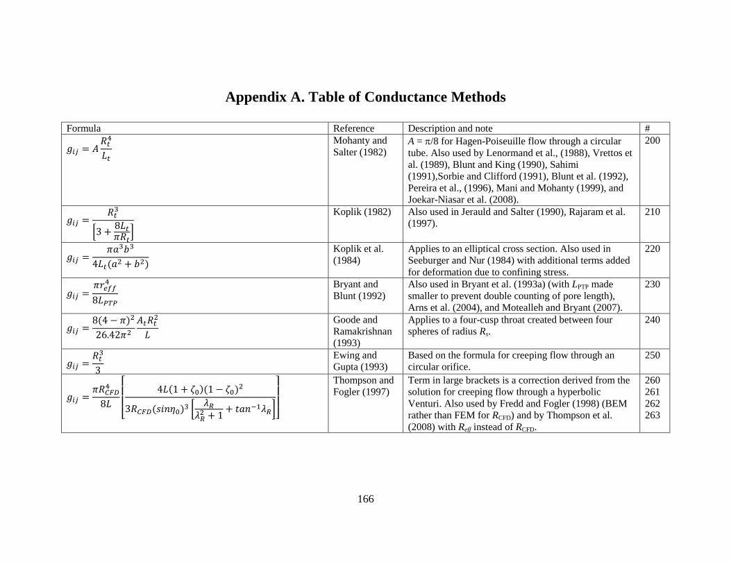
166

Appendix A. Table of Conductance Methods

Formula Reference Description and note #

Mohanty and

Salter (1982) A = /8 for Hagen-Poiseuille flow through a circular

tube. Also used by Lenormand et al., (1988), Vrettos et

al. (1989), Blunt and King (1990), Sahimi

(1991),Sorbie and Clifford (1991), Blunt et al. (1992),

Pereira et al., (1996), Mani and Mohanty (1999), and

Joekar-Niasar et al. (2008).

200

Koplik (1982) Also used in Jerauld and Salter (1990), Rajaram et al.

(1997).

210

Koplik et al.

(1984)

Applies to an elliptical cross section. Also used in

Seeburger and Nur (1984) with additional terms added

for deformation due to confining stress.

220

Bryant and

Blunt (1992)

Also used in Bryant et al. (1993a) (with LPTP made

smaller to prevent double counting of pore length),

Arns et al. (2004), and Motealleh and Bryant (2007).

230

Goode and

Ramakrishnan

(1993)

Applies to a four-cusp throat created between four

spheres of radius Rs.

240

Ewing and

Gupta (1993)

Based on the formula for creeping flow through an

circular orifice.

250

Thompson and

Fogler (1997)

Term in large brackets is a correction derived from the

solution for creeping flow through a hyperbolic

Venturi. Also used by Fredd and Fogler (1998) (BEM

rather than FEM for RCFD) and by Thompson et al.

(2008) with Reff instead of RCFD.

260

261

262

263

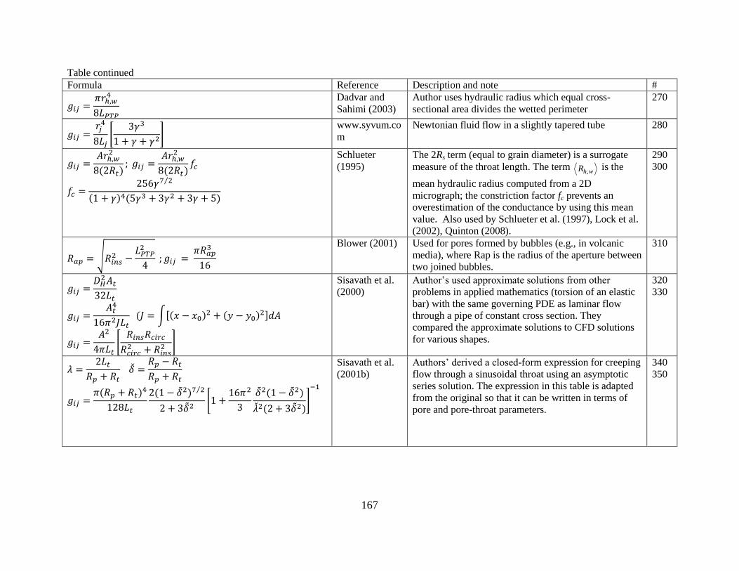
167

Table continued


Dadvar and

Sahimi (2003)

Author uses hydraulic radius which equal cross-

sectional area divides the wetted perimeter

270

www.syvum.co

m

Newtonian fluid flow in a slightly tapered tube 280

Schlueter

(1995)

The 2Rs term (equal to grain diameter) is a surrogate

measure of the throat length. The term ,h wR is the

mean hydraulic radius computed from a 2D

micrograph; the constriction factor fc prevents an

overestimation of the conductance by using this mean

value. Also used by Schlueter et al. (1997), Lock et al.

(2002), Quinton (2008).

290

300

Blower (2001) Used for pores formed by bubbles (e.g., in volcanic

media), where Rap is the radius of the aperture between

two joined bubbles.

310

Sisavath et al.

(2000)

Author’s used approximate solutions from other

problems in applied mathematics (torsion of an elastic

bar) with the same governing PDE as laminar flow

through a pipe of constant cross section. They

compared the approximate solutions to CFD solutions

for various shapes.

320

330

Sisavath et al.

(2001b)

Authors’ derived a closed-form expression for creeping

flow through a sinusoidal throat using an asymptotic

series solution. The expression in this table is adapted

from the original so that it can be written in terms of

pore and pore-throat parameters.

340

350

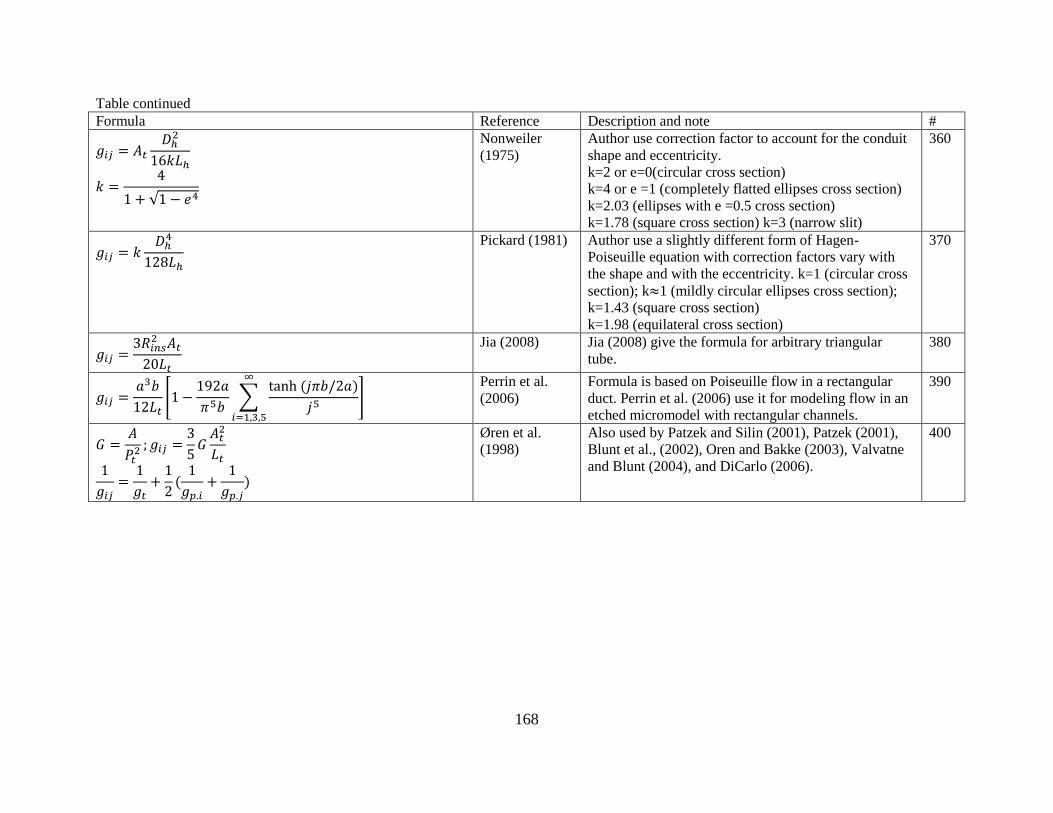
168

Table continued


Nonweiler

(1975)

Author use correction factor to account for the conduit

shape and eccentricity.

k=2 or e=0(circular cross section)

k=4 or e =1 (completely flatted ellipses cross section)

k=2.03 (ellipses with e =0.5 cross section)

k=1.78 (square cross section) k=3 (narrow slit)

360

Pickard (1981) Author use a slightly different form of Hagen-

Poiseuille equation with correction factors vary with

the shape and with the eccentricity. k=1 (circular cross

section); k 1 (mildly circular ellipses cross section);

k=1.43 (square cross section)

k=1.98 (equilateral cross section)

370

Jia (2008) Jia (2008) give the formula for arbitrary triangular

tube.

380

Perrin et al.

(2006)

Formula is based on Poiseuille flow in a rectangular

duct. Perrin et al. (2006) use it for modeling flow in an

etched micromodel with rectangular channels.

390

Øren et al.

(1998)

Also used by Patzek and Silin (2001), Patzek (2001),

Blunt et al., (2002), Oren and Bakke (2003), Valvatne

and Blunt (2004), and DiCarlo (2006).

400

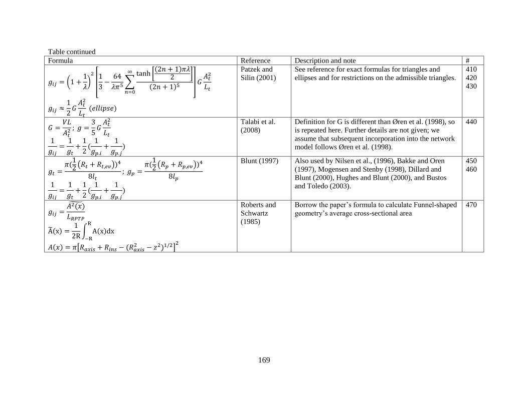
169

Table continued


Patzek and

Silin (2001)

See reference for exact formulas for triangles and

ellipses and for restrictions on the admissible triangles.

410

420

430

Talabi et al.

(2008)

Definition for G is different than Øren et al. (1998), so

is repeated here. Further details are not given; we

assume that subsequent incorporation into the network

model follows Øren et al. (1998).

440

Blunt (1997) Also used by Nilsen et al., (1996), Bakke and Oren

(1997), Mogensen and Stenby (1998), Dillard and

Blunt (2000), Hughes and Blunt (2000), and Bustos

and Toledo (2003).

450

460

Roberts and

Schwartz

(1985)

Borrow the paper’s formula to calculate Funnel-shaped

geometry’s average cross-sectional area

470

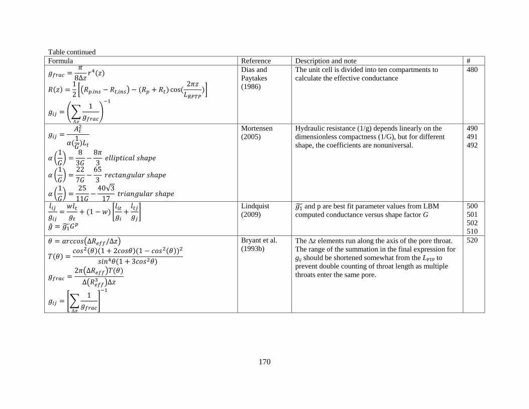
170

Table continued


Dias and

Paytakes

(1986)

The unit cell is divided into ten compartments to

calculate the effective conductance

480

Mortensen

(2005)

Hydraulic resistance (1/g) depends linearly on the

dimensionless compactness (1/G), but for different

shape, the coefficients are nonuniversal.

490

491

492

Lindquist

(2009) and p are best fit parameter values from LBM

computed conductance versus shape factor G

500

501

502

510

Bryant et al.

(1993b) The z elements run along the axis of the pore throat.

The range of the summation in the final expression for

gij should be shortened somewhat from the LPTP to

prevent double counting of throat length as multiple

throats enter the same pore.

520

171

Table continued


Ioannidis and

Chatzis (1993)

Applies to a rectangular cross section. Also used by

Pan et al., (2001), Talukdar et al. (2002) (with throat

resistance only), and Gostick et al. (2007).

530

Celia(2006) The conductance is sampled from the log-normal

distribution with mean and variance ,

which depend on the log-volume summation

as they assume strong correlation between

conductance and adjacent pore volumes

540

Matthews(1993

)

Each pore-throat-pore connection in the network

consists of three components: a throat and half of each

adjoining pore

The second equation is for gas with slip correction, s is

a constant which may vary with temperature, capillary

and molecular species

550

Aker (1998) K is the permeability. Also used by Matthews (1993),

Knudsen (2002).

560

Payatakes and

Flumerfelt

(1980)

The parameter c2 is measured experimentally (Dias and

Paytakes, 1986). Hence, this conductance equation

requires additional information apart from the usual

geometric parameters describing the network. Also

used in Lin and Slattery (1982), Dias and Payatakes

(1986), and Hopkins and Ng (1986).

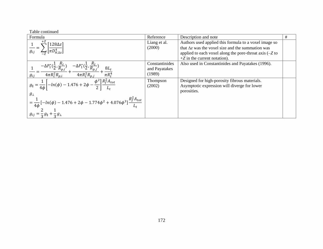
172

Table continued


Liang et al.

(2000)

Authors used applied this formula to a voxel image so

that z was the voxel size and the summation was

applied to each voxel along the pore-throat axis (–Z to

+Z in the current notation).

Constantinides

and Payatakes

(1989)

Also used in Constantinides and Payatakes (1996).

Thompson

(2002)

Designed for high-porosity fibrous materials.

Asymptotic expression will diverge for lower

porosities.

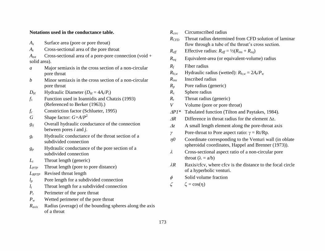
173

Notations used in the conductance table.

As Surface area (pore or pore throat)

At Cross-sectional area of the pore throat

Atot Cross-sectional area of a pore-pore connection (void +

solid area).

a Major semiaxis in the cross section of a non-circular

pore throat

b Minor semiaxis in the cross section of a non-circular

pore throat

DH Hydraulic Diameter (DH = 4At/Pt)

f1 Function used in Ioannidis and Chatzis (1993)

(Referenced to Berker (1963).)

fc Constriction factor (Schlueter, 1995)

G Shape factor: G=A/P2

gij Overall hydraulic conductance of the connection

between pores i and j.

gt Hydraulic conductance of the throat section of a

subdivided connection

gp Hydraulic conductance of the pore section of a

subdivided connection

Lt Throat length (generic)

LPTP Throat length (pore to pore distance)

LRPTP Revised throat length

lp Pore length for a subdivided connection

lt Throat length for a subdivided connection

Pt Perimeter of the pore throat

Pw Wetted perimeter of the pore throat

Raxis Radius (average) of the bounding spheres along the axis

of a throat

Rcirc Circumscribed radius

RCFD Throat radius determined from CFD solution of laminar

flow through a tube of the throat’s cross section.

Reff Effective radius: Reff = ½(Rins + Req)

Req Equivalent-area (or equivalent-volume) radius

Rf Fiber radius

Rh,w Hydraulic radius (wetted): Rh,w = 2At/Pw

Rins Inscribed radius

Rp Pore radius (generic)

Rs Sphere radius

Rt Throat radius (generic)

V Volume (pore or pore throat)

P1* Tabulated function (Tilton and Paytakes, 1984).

R Difference in throat radius for the element z.

z A small length element along the pore-throat axis

Pore-throat to Pore aspect ratio: = Rt/Rp.

0 Coordinate corresponding to the Venturi wall (in oblate

spheroidal coordinates, Happel and Brenner (1973)).

Cross-sectional aspect ratio of a non-circular pore

throat ( = a/b)

R Raxis/cfcv, where cfcv is the distance to the focal circle

of a hyperbolic venturi.

Solid volume fraction

= cos()

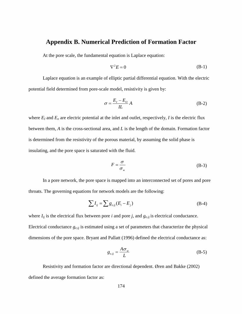
174

Appendix B. Numerical Prediction of Formation Factor

At the pore scale, the fundamental equation is Laplace equation:

02 E (B-1)

Laplace equation is an example of elliptic partial differential equation. With the electric

potential field determined from pore-scale model, resistivity is given by:

AIL

EE OI (B-2)

where EI and Eo are electric potential at the inlet and outlet, respectively, I is the electric flux

between them, A is the cross-sectional area, and L is the length of the domain. Formation factor

is determined from the resistivity of the porous material, by assuming the solid phase is

insulating, and the pore space is saturated with the fluid.

w

F

(B-3)

In a pore network, the pore space is mapped into an interconnected set of pores and pore

throats. The governing equations for network models are the following:

)(, jiijeij EEgI (B-4)

where Iij is the electrical flux between pore i and pore j, and ge,ij is electrical conductance.

Electrical conductance ge,ij is estimated using a set of parameters that characterize the physical

dimensions of the pore space. Bryant and Pallatt (1996) defined the electrical conductance as:

L

Ag w

ije

, (B-5)

Resistivity and formation factor are directional dependent. Øren and Bakke (2002)

defined the average formation factor as:

175

)111

(3

11

zyx FFFF (B-6)

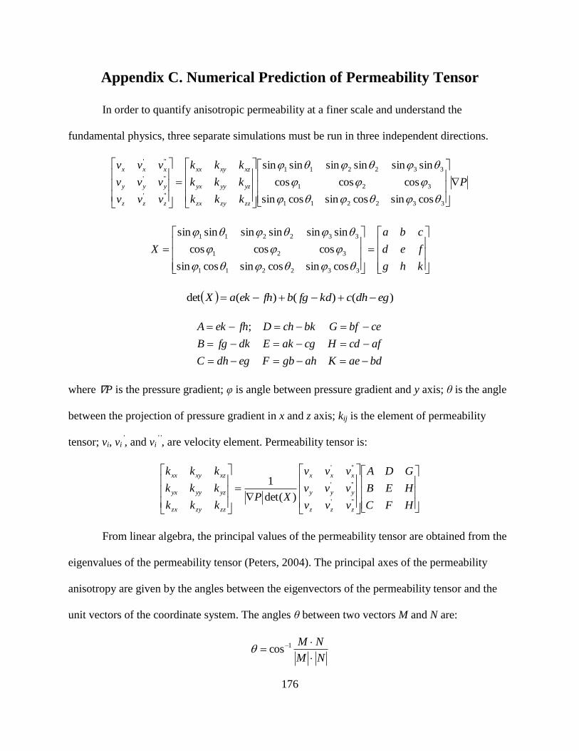
176

Appendix C. Numerical Prediction of Permeability Tensor

In order to quantify anisotropic permeability at a finer scale and understand the

fundamental physics, three separate simulations must be run in three independent directions.

P

kkk

kkk

kkk

vvv

vvv

vvv

zzzyzx

yzyyyx

xzxyxx

zzz

yyy

xxx

332211

321

332211

'''

'''

'''

cossincossincossin

coscoscos

sinsinsinsinsinsin

khg

fed

cba

X

332211

321

332211

cossincossincossin

coscoscos

sinsinsinsinsinsin

)()()(det egdhckdfgbfhekaX

bdaeKahgbFegdhC

afcdHcgakEdkfgB

cebfGbkchDfhekA

;

where ∇P is the pressure gradient; φ is angle between pressure gradient and y axis; θ is the angle

between the projection of pressure gradient in x and z axis; kij is the element of permeability

tensor; vi, vi’, and vi

’’, are velocity element. Permeability tensor is:

HFC

HEB

GDA

vvv

vvv

vvv

XPkkk

kkk

kkk

zzz

yyy

xxx

zzzyzx

yzyyyx

xzxyxx

'''

'''

'''

)det(

1

From linear algebra, the principal values of the permeability tensor are obtained from the

eigenvalues of the permeability tensor (Peters, 2004). The principal axes of the permeability

anisotropy are given by the angles between the eigenvectors of the permeability tensor and the

unit vectors of the coordinate system. The angles θ between two vectors M and N are:

NM

NM

1cos

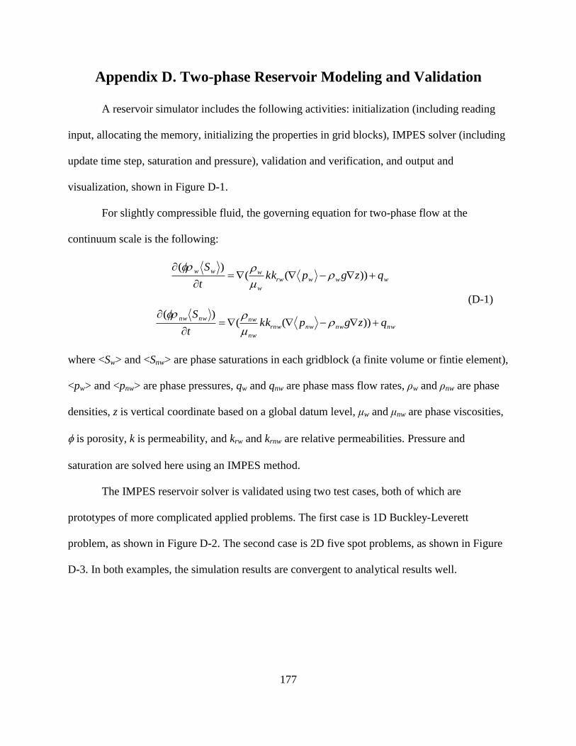
177

Appendix D. Two-phase Reservoir Modeling and Validation

A reservoir simulator includes the following activities: initialization (including reading

input, allocating the memory, initializing the properties in grid blocks), IMPES solver (including

update time step, saturation and pressure), validation and verification, and output and

visualization, shown in Figure D-1.

For slightly compressible fluid, the governing equation for two-phase flow at the

continuum scale is the following:

wwwrw

w

wwwqzgpkk

t

S

))((

)(

(D-1)

nwnwnwrnw

nw

nwnwnwqzgpkk

t

S

))((

)(

where <Sw> and <Snw> are phase saturations in each gridblock (a finite volume or fintie element),

<pw> and <pnw> are phase pressures, qw and qnw are phase mass flow rates, ρw and ρnw are phase

densities, z is vertical coordinate based on a global datum level, μw and μnw are phase viscosities,

is porosity, k is permeability, and krw and krnw are relative permeabilities. Pressure and

saturation are solved here using an IMPES method.

The IMPES reservoir solver is validated using two test cases, both of which are

prototypes of more complicated applied problems. The first case is 1D Buckley-Leverett

problem, as shown in Figure D-2. The second case is 2D five spot problems, as shown in Figure

D-3. In both examples, the simulation results are convergent to analytical results well.

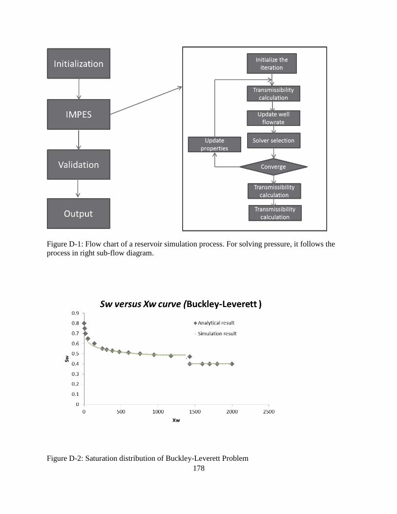
178

Figure D-1: Flow chart of a reservoir simulation process. For solving pressure, it follows the

process in right sub-flow diagram.

Figure D-2: Saturation distribution of Buckley-Leverett Problem

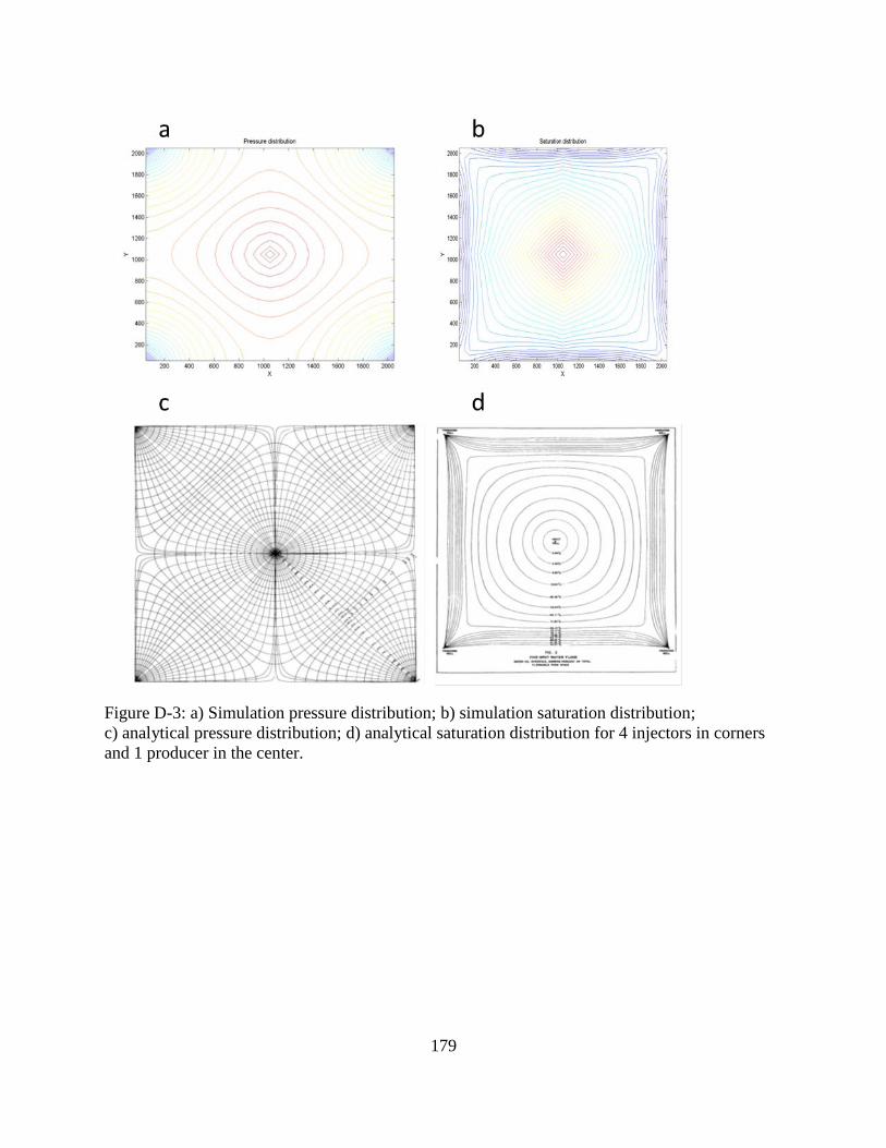
179

Figure D-3: a) Simulation pressure distribution; b) simulation saturation distribution;

c) analytical pressure distribution; d) analytical saturation distribution for 4 injectors in corners

and 1 producer in the center.

180

Vita

Qiang Sheng was born and raised in Zibo, Shandong Province, China. He

attended Zibo No. 1 high school and received his diploma in 2000. He went to Tianjin

University and graduated with degrees in Bachelor of Science in Chemical Engineering

and Financial Management in June 2004. He then studied and worked in Shanghai

Research Institute of Chemical Industry for three years. In August, 2007, he was accepted

as a doctoral candidate by the Department of Chemical Engineering, Louisiana State

University-Baton Rouge.

Documents

Pore-to-continuum Multiscale Modeling of Two-phase Flow in