Embed Size (px)
Citation preview
MARKETING RESEARCH
Assignment No : 3
Submitted by
K.NARESH KUMAR (172)
Section-C
PGDM-General
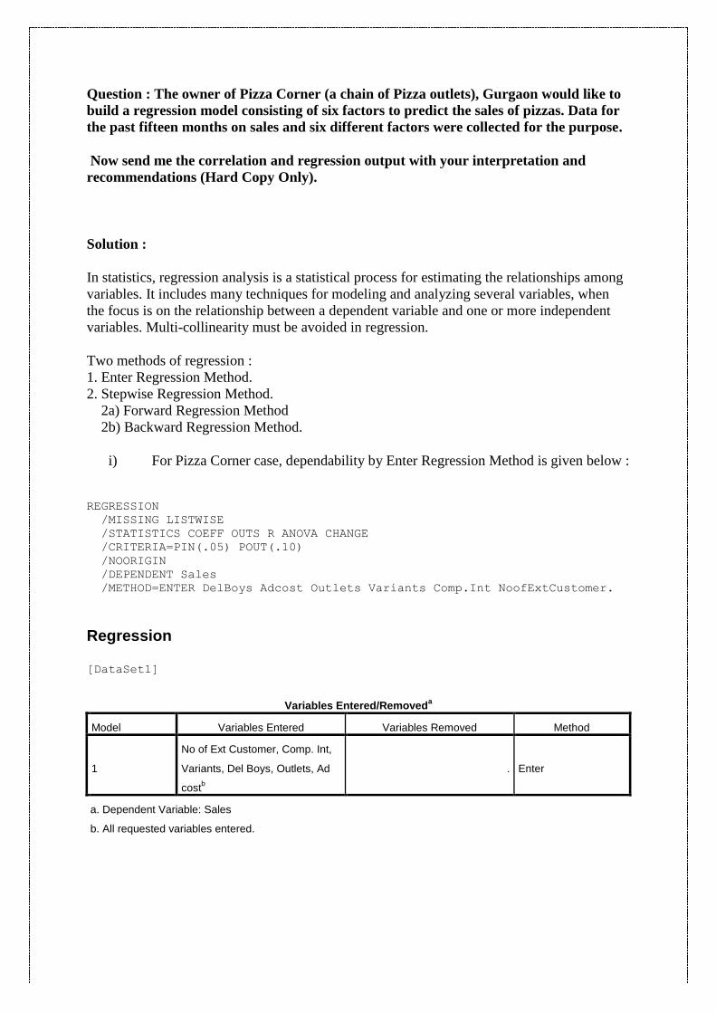
Question : The owner of Pizza Corner (a chain of Pizza outlets), Gurgaon would like to
build a regression model consisting of six factors to predict the sales of pizzas. Data for
the past fifteen months on sales and six different factors were collected for the purpose.
Now send me the correlation and regression output with your interpretation and
recommendations (Hard Copy Only).
Solution :
In statistics, regression analysis is a statistical process for estimating the relationships among
variables. It includes many techniques for modeling and analyzing several variables, when
the focus is on the relationship between a dependent variable and one or more independent
variables. Multi-collinearity must be avoided in regression.
Two methods of regression :
1. Enter Regression Method.
2. Stepwise Regression Method.
2a) Forward Regression Method
2b) Backward Regression Method.
i) For Pizza Corner case, dependability by Enter Regression Method is given below :
REGRESSION
/MISSING LISTWISE
/STATISTICS COEFF OUTS R ANOVA CHANGE
/CRITERIA=PIN(.05) POUT(.10)
/NOORIGIN
/DEPENDENT Sales
/METHOD=ENTER DelBoys Adcost Outlets Variants Comp.Int NoofExtCustomer.
Regression [DataSet1]
Variables Entered/Removeda
Model Variables Entered Variables Removed Method
1
No of Ext Customer, Comp. Int,
Variants, Del Boys, Outlets, Ad
costb
. Enter
a. Dependent Variable: Sales
b. All requested variables entered.
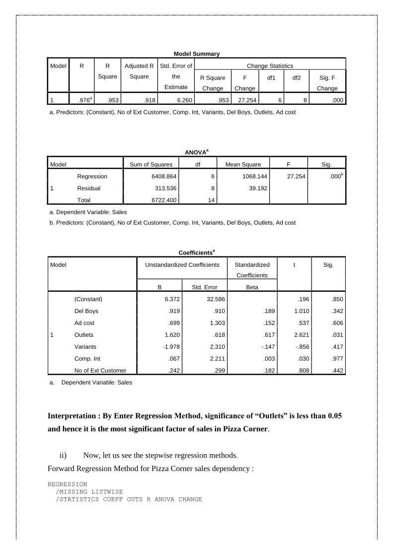
Model Summary
Model R R
Square
Adjusted R
Square
Std. Error of
the
Estimate
Change Statistics
R Square
Change
F
Change
df1 df2 Sig. F
Change
1 .976a .953 .918 6.260 .953 27.254 6 8 .000
a. Predictors: (Constant), No of Ext Customer, Comp. Int, Variants, Del Boys, Outlets, Ad cost
ANOVAa
Model Sum of Squares df Mean Square F Sig.
1
Regression 6408.864 6 1068.144 27.254 .000b
Residual 313.536 8 39.192
Total 6722.400 14
a. Dependent Variable: Sales
b. Predictors: (Constant), No of Ext Customer, Comp. Int, Variants, Del Boys, Outlets, Ad cost
Coefficientsa
Model Unstandardized Coefficients Standardized
Coefficients
t Sig.
B Std. Error Beta
1
(Constant) 6.372 32.586 .196 .850
Del Boys .919 .910 .189 1.010 .342
Ad cost .699 1.303 .152 .537 .606
Outlets 1.620 .618 .617 2.621 .031
Variants -1.978 2.310 -.147 -.856 .417
Comp. Int .067 2.211 .003 .030 .977
No of Ext Customer .242 .299 .182 .808 .442
a. Dependent Variable: Sales
Interpretation : By Enter Regression Method, significance of “Outlets” is less than 0.05
and hence it is the most significant factor of sales in Pizza Corner.
ii) Now, let us see the stepwise regression methods.
Forward Regression Method for Pizza Corner sales dependency :
REGRESSION
/MISSING LISTWISE
/STATISTICS COEFF OUTS R ANOVA CHANGE
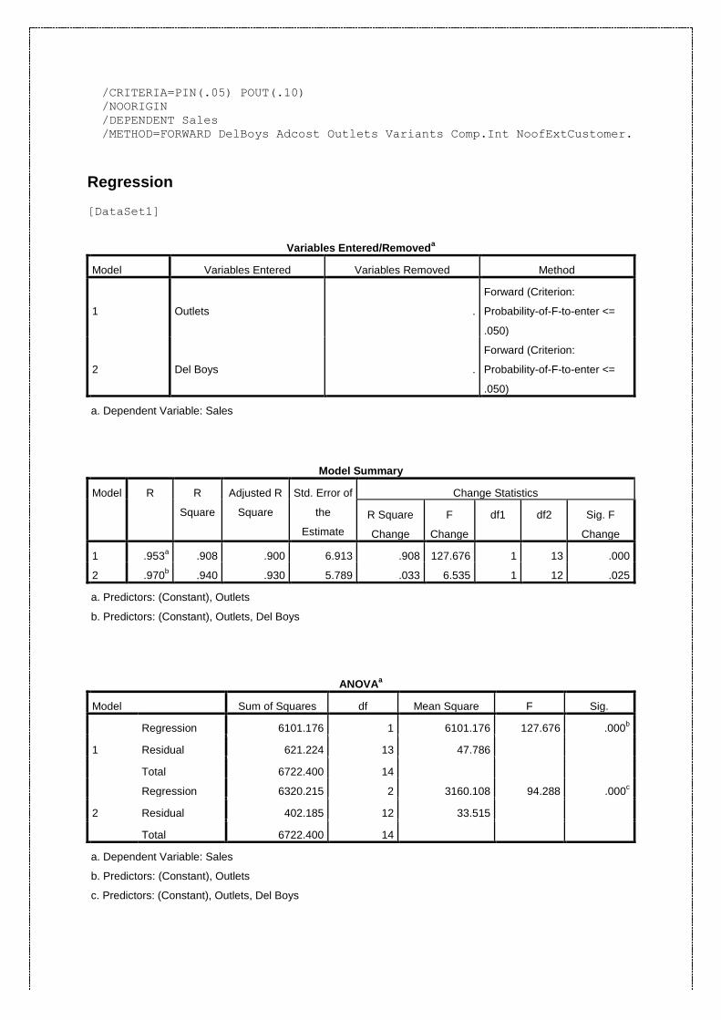
/CRITERIA=PIN(.05) POUT(.10)
/NOORIGIN
/DEPENDENT Sales
/METHOD=FORWARD DelBoys Adcost Outlets Variants Comp.Int NoofExtCustomer.
Regression
[DataSet1]
Variables Entered/Removeda
Model Variables Entered Variables Removed Method
1 Outlets .
Forward (Criterion:
Probability-of-F-to-enter <=
.050)
2 Del Boys .
Forward (Criterion:
Probability-of-F-to-enter <=
.050)
a. Dependent Variable: Sales
Model Summary
Model R R
Square
Adjusted R
Square
Std. Error of
the
Estimate
Change Statistics
R Square
Change
F
Change
df1 df2 Sig. F
Change
1 .953a .908 .900 6.913 .908 127.676 1 13 .000
2 .970b .940 .930 5.789 .033 6.535 1 12 .025
a. Predictors: (Constant), Outlets
b. Predictors: (Constant), Outlets, Del Boys
ANOVAa
Model Sum of Squares df Mean Square F Sig.
1
Regression 6101.176 1 6101.176 127.676 .000b
Residual 621.224 13 47.786
Total 6722.400 14
2
Regression 6320.215 2 3160.108 94.288 .000c
Residual 402.185 12 33.515
Total 6722.400 14
a. Dependent Variable: Sales
b. Predictors: (Constant), Outlets
c. Predictors: (Constant), Outlets, Del Boys
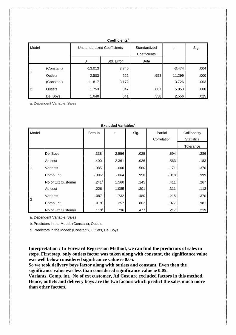
Coefficientsa
Model Unstandardized Coefficients Standardized
Coefficients
t Sig.
B Std. Error Beta
1 (Constant) -13.013 3.746 -3.474 .004
Outlets 2.503 .222 .953 11.299 .000
2
(Constant) -11.817 3.172 -3.726 .003
Outlets 1.753 .347 .667 5.053 .000
Del Boys 1.640 .641 .338 2.556 .025
a. Dependent Variable: Sales
Excluded Variablesa
Model Beta In t Sig. Partial
Correlation
Collinearity
Statistics
Tolerance
1
Del Boys .338b 2.556 .025 .594 .286
Ad cost .400b 2.361 .036 .563 .183
Variants -.085b -.600 .560 -.171 .370
Comp. Int -.006b -.064 .950 -.018 .999
No of Ext Customer .241b 1.560 .145 .411 .267
2
Ad cost .226c 1.085 .301 .311 .113
Variants -.087c -.732 .480 -.215 .370
Comp. Int .019c .257 .802 .077 .981
No of Ext Customer .113c .736 .477 .217 .219
a. Dependent Variable: Sales
b. Predictors in the Model: (Constant), Outlets
c. Predictors in the Model: (Constant), Outlets, Del Boys
Interpretation : In Forward Regression Method, we can find the predictors of sales in
steps. First step, only outlets factor was taken along with constant, the significance value
was well below considered significance value ie 0.05.
So we took delivery boys factor along with outlets and constant. Even then the
significance value was less than considered significance value ie 0.05.
Variants, Comp. int., No of ext customer, Ad Cost are excluded factors in this method.
Hence, outlets and delivery boys are the two factors which predict the sales much more
than other factors.
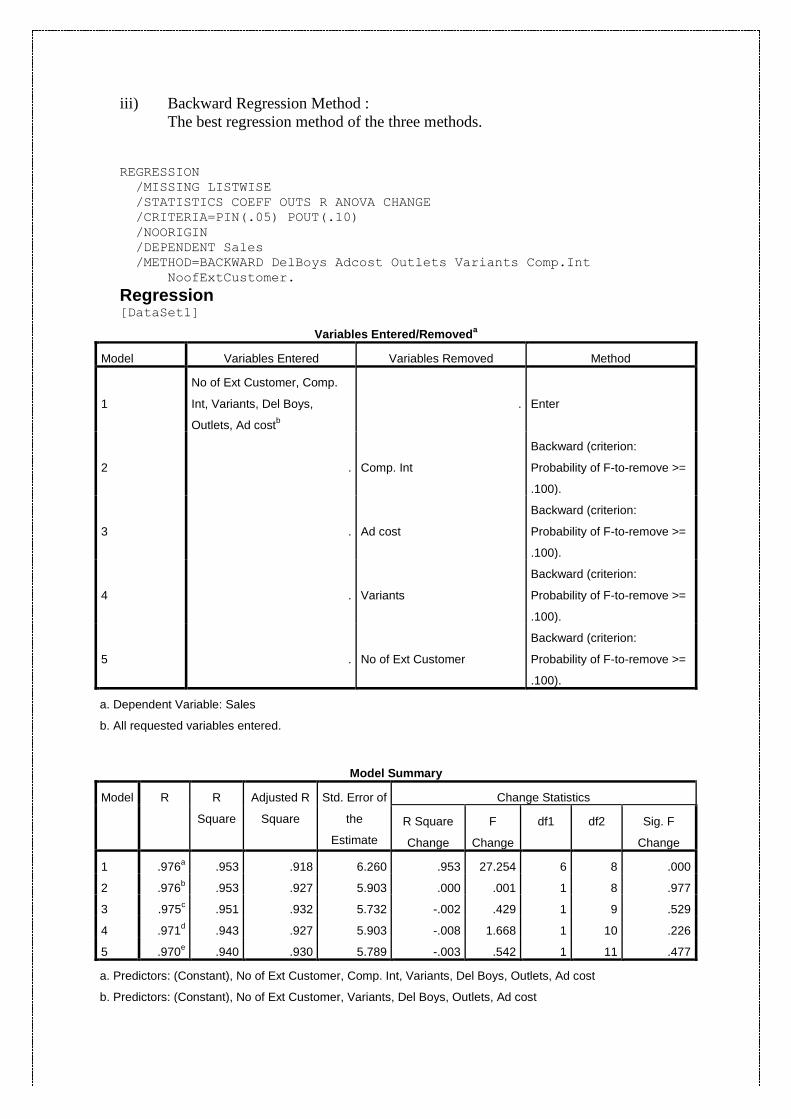
iii) Backward Regression Method :
The best regression method of the three methods.
REGRESSION
/MISSING LISTWISE
/STATISTICS COEFF OUTS R ANOVA CHANGE
/CRITERIA=PIN(.05) POUT(.10)
/NOORIGIN
/DEPENDENT Sales
/METHOD=BACKWARD DelBoys Adcost Outlets Variants Comp.Int
NoofExtCustomer.
Regression [DataSet1]
Variables Entered/Removeda
Model Variables Entered Variables Removed Method
1
No of Ext Customer, Comp.
Int, Variants, Del Boys,
Outlets, Ad costb
. Enter
2 . Comp. Int
Backward (criterion:
Probability of F-to-remove >=
.100).
3 . Ad cost
Backward (criterion:
Probability of F-to-remove >=
.100).
4 . Variants
Backward (criterion:
Probability of F-to-remove >=
.100).
5 . No of Ext Customer
Backward (criterion:
Probability of F-to-remove >=
.100).
a. Dependent Variable: Sales
b. All requested variables entered.
Model Summary
Model R R
Square
Adjusted R
Square
Std. Error of
the
Estimate
Change Statistics
R Square
Change
F
Change
df1 df2 Sig. F
Change
1 .976a .953 .918 6.260 .953 27.254 6 8 .000
2 .976b .953 .927 5.903 .000 .001 1 8 .977
3 .975c .951 .932 5.732 -.002 .429 1 9 .529
4 .971d .943 .927 5.903 -.008 1.668 1 10 .226
5 .970e .940 .930 5.789 -.003 .542 1 11 .477
a. Predictors: (Constant), No of Ext Customer, Comp. Int, Variants, Del Boys, Outlets, Ad cost
b. Predictors: (Constant), No of Ext Customer, Variants, Del Boys, Outlets, Ad cost
c. Predictors: (Constant), No of Ext Customer, Variants, Del Boys, Outlets
d. Predictors: (Constant), No of Ext Customer, Del Boys, Outlets
e. Predictors: (Constant), Del Boys, Outlets
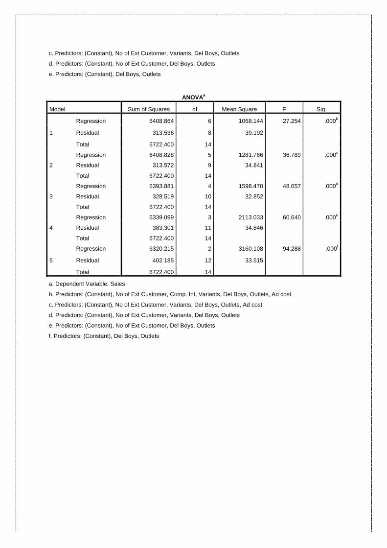
ANOVAa
Model Sum of Squares df Mean Square F Sig.
1
Regression 6408.864 6 1068.144 27.254 .000b
Residual 313.536 8 39.192
Total 6722.400 14
2
Regression 6408.828 5 1281.766 36.789 .000c
Residual 313.572 9 34.841
Total 6722.400 14
3
Regression 6393.881 4 1598.470 48.657 .000d
Residual 328.519 10 32.852
Total 6722.400 14
4
Regression 6339.099 3 2113.033 60.640 .000e
Residual 383.301 11 34.846
Total 6722.400 14
5
Regression 6320.215 2 3160.108 94.288 .000f
Residual 402.185 12 33.515
Total 6722.400 14
a. Dependent Variable: Sales
b. Predictors: (Constant), No of Ext Customer, Comp. Int, Variants, Del Boys, Outlets, Ad cost
c. Predictors: (Constant), No of Ext Customer, Variants, Del Boys, Outlets, Ad cost
d. Predictors: (Constant), No of Ext Customer, Variants, Del Boys, Outlets
e. Predictors: (Constant), No of Ext Customer, Del Boys, Outlets
f. Predictors: (Constant), Del Boys, Outlets
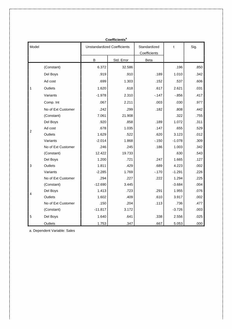
Coefficientsa
Model Unstandardized Coefficients Standardized
Coefficients
t Sig.
B Std. Error Beta
1
(Constant) 6.372 32.586 .196 .850
Del Boys .919 .910 .189 1.010 .342
Ad cost .699 1.303 .152 .537 .606
Outlets 1.620 .618 .617 2.621 .031
Variants -1.978 2.310 -.147 -.856 .417
Comp. Int .067 2.211 .003 .030 .977
No of Ext Customer .242 .299 .182 .808 .442
2
(Constant) 7.061 21.908 .322 .755
Del Boys .920 .858 .189 1.072 .311
Ad cost .678 1.035 .147 .655 .529
Outlets 1.629 .522 .620 3.123 .012
Variants -2.014 1.868 -.150 -1.078 .309
No of Ext Customer .246 .245 .186 1.003 .342
3
(Constant) 12.422 19.733 .630 .543
Del Boys 1.200 .721 .247 1.665 .127
Outlets 1.811 .429 .689 4.223 .002
Variants -2.285 1.769 -.170 -1.291 .226
No of Ext Customer .294 .227 .222 1.294 .225
4
(Constant) -12.690 3.445 -3.684 .004
Del Boys 1.413 .723 .291 1.955 .076
Outlets 1.602 .409 .610 3.917 .002
No of Ext Customer .150 .204 .113 .736 .477
5
(Constant) -11.817 3.172 -3.726 .003
Del Boys 1.640 .641 .338 2.556 .025
Outlets 1.753 .347 .667 5.053 .000
a. Dependent Variable: Sales
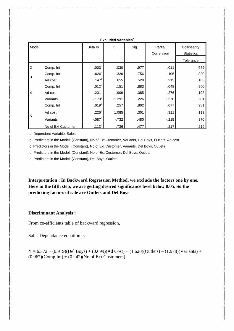
Excluded Variablesa
Model Beta In t Sig. Partial
Correlation
Collinearity
Statistics
Tolerance
2 Comp. Int .003b .030 .977 .011 .589
3 Comp. Int -.026
c -.320 .756 -.106 .830
Ad cost .147c .655 .529 .213 .103
4
Comp. Int .012d .151 .883 .048 .960
Ad cost .201d .909 .385 .276 .108
Variants -.170d -1.291 .226 -.378 .281
5
Comp. Int .019e .257 .802 .077 .981
Ad cost .226e 1.085 .301 .311 .113
Variants -.087e -.732 .480 -.215 .370
No of Ext Customer .113e .736 .477 .217 .219
a. Dependent Variable: Sales
b. Predictors in the Model: (Constant), No of Ext Customer, Variants, Del Boys, Outlets, Ad cost
c. Predictors in the Model: (Constant), No of Ext Customer, Variants, Del Boys, Outlets
d. Predictors in the Model: (Constant), No of Ext Customer, Del Boys, Outlets
e. Predictors in the Model: (Constant), Del Boys, Outlets
Interpretation : In Backward Regression Method, we exclude the factors one by one.
Here in the fifth step, we are getting desired significance level below 0.05. So the
predicting factors of sale are Outlets and Del Boys.
Discriminant Analysis :
From co-efficients table of backward regression,
Sales Dependance equation is
Y = 6.372 + (0.919)(Del Boys) + (0.699)(Ad Cost) + (1.620)(Outlets) – (1.978)(Variants) +
(0.067)(Comp Int) + (0.242)(No of Ext Customers)
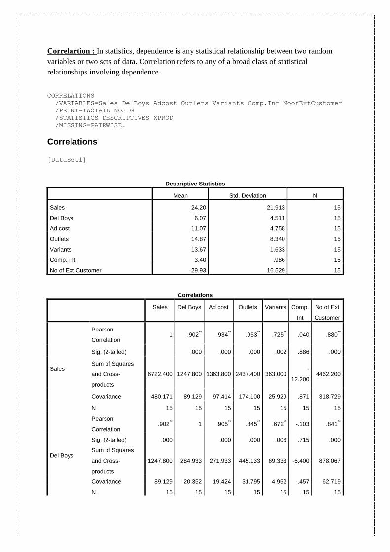
Correlartion : In statistics, dependence is any statistical relationship between two random
variables or two sets of data. Correlation refers to any of a broad class of statistical
relationships involving dependence.
CORRELATIONS
/VARIABLES=Sales DelBoys Adcost Outlets Variants Comp.Int NoofExtCustomer
/PRINT=TWOTAIL NOSIG
/STATISTICS DESCRIPTIVES XPROD
/MISSING=PAIRWISE.
Correlations [DataSet1]
Descriptive Statistics
Mean Std. Deviation N
Sales 24.20 21.913 15
Del Boys 6.07 4.511 15
Ad cost 11.07 4.758 15
Outlets 14.87 8.340 15
Variants 13.67 1.633 15
Comp. Int 3.40 .986 15
No of Ext Customer 29.93 16.529 15
Correlations
Sales Del Boys Ad cost Outlets Variants Comp.
Int
No of Ext
Customer
Sales
Pearson
Correlation 1 .902
** .934
** .953
** .725
** -.040 .880
**
Sig. (2-tailed) .000 .000 .000 .002 .886 .000
Sum of Squares
and Cross-
products
6722.400 1247.800 1363.800 2437.400 363.000 -
12.200 4462.200
Covariance 480.171 89.129 97.414 174.100 25.929 -.871 318.729
N 15 15 15 15 15 15 15
Del Boys
Pearson
Correlation .902
** 1 .905
** .845
** .672
** -.103 .841
**
Sig. (2-tailed) .000 .000 .000 .006 .715 .000
Sum of Squares
and Cross-
products
1247.800 284.933 271.933 445.133 69.333 -6.400 878.067
Covariance 89.129 20.352 19.424 31.795 4.952 -.457 62.719
N 15 15 15 15 15 15 15
Ad cost
Pearson
Correlation .934
** .905
** 1 .904
** .702
** -.189 .867
**
Sig. (2-tailed) .000 .000 .000 .004 .500 .000
Sum of Squares
and Cross-
products
1363.800 271.933 316.933 502.133 76.333 -
12.400 954.067
Covariance 97.414 19.424 22.638 35.867 5.452 -.886 68.148
N 15 15 15 15 15 15 15
Outlets
Pearson
Correlation .953
** .845
** .904
** 1 .794
** -.036 .856
**
Sig. (2-tailed) .000 .000 .000 .000 .897 .000
Sum of Squares
and Cross-
products
2437.400 445.133 502.133 973.733 151.333 -4.200 1651.867
Covariance 174.100 31.795 35.867 69.552 10.810 -.300 117.990
N 15 15 15 15 15 15 15
Variants
Pearson
Correlation .725
** .672
** .702
** .794
** 1 -.178 .819
**
Sig. (2-tailed) .002 .006 .004 .000 .527 .000
Sum of Squares
and Cross-
products
363.000 69.333 76.333 151.333 37.333 -4.000 309.667
Covariance 25.929 4.952 5.452 10.810 2.667 -.286 22.119
N 15 15 15 15 15 15 15
Comp. Int
Pearson
Correlation -.040 -.103 -.189 -.036 -.178 1 .006
Sig. (2-tailed) .886 .715 .500 .897 .527 .983
Sum of Squares
and Cross-
products
-12.200 -6.400 -12.400 -4.200 -4.000 13.600 1.400
Covariance -.871 -.457 -.886 -.300 -.286 .971 .100
N 15 15 15 15 15 15 15
No of Ext
Customer
Pearson
Correlation .880
** .841
** .867
** .856
** .819
** .006 1
Sig. (2-tailed) .000 .000 .000 .000 .000 .983
Sum of Squares
and Cross-
products
4462.200 878.067 954.067 1651.867 309.667 1.400 3824.933
Covariance 318.729 62.719 68.148 117.990 22.119 .100 273.210
N 15 15 15 15 15 15 15
**. Correlation is significant at the 0.01 level (2-tailed).
Interpretation : According to Correlation coefficients table, Sales have a positive
relationship with Outlets, Del boys , Ad cost, No of ext customers and variants. While
sales have negative relationship (dependence) with Comp Int.
Controlling other variables constant, if Number of delivery boys is increased by 1 then Sales
will increase by 0.919
Controlling other variables constant, if of ad cost is increased by 1 then
Sales will increase by 0.699
Controlling other variables constant, if Number of outlets is increased by 1 then Sales will
increase by 1.620
Controlling other variables constant, if variants of pizza is increased by 1 then Sales will
decrease by 1.978
Controlling other variables constant, if Competitors’ index is increased by 1 then sales will
increase by 0.067
Controlling other variables constant, if Number of existing customers is increased by 1 then
sales will increase by 0.242
RECOMMENDATIONS :
1. Increase the no. of delivery boys.
2. Increase the pizza outlets.
3. Reduce the expense on competitors’ index.
4. Variants don’t have any significant effect on sales, so don’t spend much on variants.