Paying is Believing: The E¤ect of Costly Information on

Bayesian Updating�

Pedro Robalo

University of Amsterdam

Tinbergen Institute

Rei Sayagy

Erasmus University Rotterdam

Tinbergen Institute

February 2013

Abstract

The supposed irrelevance of historical costs for rational decision making has been the sub-

ject of much interest in the economic literature. In this paper we explore whether individual

decision making under risk is a¤ected by the cost of information. To do so one must dis-

tinguish the e¤ect of cost from self selection by individuals who value information the most.

Outside of the laboratory it is di¢ cult to disentangle these two e¤ects. We thus create an

experimental environment where subjects are o¤ered additional, useful and identical infor-

mation on the state of the world across treatments. We �nd a systematic e¤ect of sunk costs

on the manner in which subjects update their beliefs. Subjects over-weigh costly information

relatively to free information, which results in a �push�of beliefs towards the extremes. This

shift does not necessarily lead to behavior more attuned with Bayesian updating. We �nd

that an intensi�cation of representativeness bias due to cost is the most likely explanation of

our results.

Keywords: sunk cost; information; Bayesian updating; decision making under risk;

heuristics and biases.

JEL codes: C91; D81; D83.

�A previous version of this paper was circulated under the title "Information at a Cost".yFor their useful comments, we would like to thank Johannes Abeler, José Apesteguia, Christoph Brunner, Gary

Charness, Dan Levin, John List, Theo O¤erman, Ariel Rubinstein, Sally Sado¤, Arthur Schram, Bauke Visser andseminar participants at the University of Amsterdam; Erasmus University Rotterdam; the Tinbergen Institute,Amsterdam; MBEES 2012, University of Maastricht; CCC 2012, University of East Anglia; the Economic ScienceAssociation Conference 2012, New York; and the Choice Lab, Norwegian School of Economics. Financial supportby the Priority Research Area Behavioral Economics of the University of Amsterdam and the Erasmus UniversityTrustfonds is gratefully acknowledged. Robalo acknowledges �nancial support from Fundação para a Ciência eTecnologia through Grant SFRH/BD/43843/2008. Sayag (corresponding author): Erasmus School of Economics,Burg. Oudlaan 50, 3062 PA Rotterdam, the Netherlands . E-mail: sayag@ese.eur.nl. Robalo: CREED, AmsterdamSchool of Economics, Roetersstraat 11, 1018 WB Amsterdam, the Netherlands. E-mail: p.robalo@uva.nl.

1

1 Introduction

Information plays a crucial role in supporting decisions made by individuals and organizations.

This paper investigates whether the cost paid for information in�uences the way it is used in

decision making. As an illustration, consider a region at risk of pandemic. Assume that a simple

and e¤ective prevention method exists (washing your hands twice a day, for example). The local

authorities simply have to make sure that knowledge of this prevention method reaches individual

citizens, i.e. they have to make citizens aware of this information (through the distribution of a

lea�et, for example). Assuming that the cost of doing so is negligible compared to the welfare gains,

should the authorities distribute the information for free or charge for it? Conditional on receiving

the information, the behavior of a rational individual should not depend on the price paid for it.

However, we conjecture otherwise: decision makers might put a higher weight on information they

had to pay for, and paying for information can interact with optimization behavior. If this is true,

a possible policy implication is that the cost of information can be used to steer decision makers�

behavior in the preferred direction.

Underlying our conjecture is the possibility that individuals fall prey to a variant of the sunk

cost e¤ect (Thaler 1980), and "use" information relatively more when it comes at a cost.1 We

contribute to the accumulated evidence on the sunk cost fallacy by investigating the existence of

sunk costs in a scenario of decision making under risk. If a relationship between information costs

and decision making exists, a follow-up question is whether it leads to better decisions. We set out

to investigate these matters using a laboratory experiment. Field data is likely to be contaminated

by serious selection issues: individuals who choose to acquire information in the �eld are likely to

di¤er along several dimensions from individuals who choose not to do so. The laboratory allows us

to correct for these selection issues through carefully constructed procedures. One way in which

we disentangle selection from sunk cost e¤ects is by imposing the cost of information on subjects.

This is something that is easily done in the laboratory, but arguably di¢ cult to implement in

the �eld.2 Moreover, the laboratory allows us to assess the extent to which individuals value

information and are able to use it; in other words, we can identify di¤erent types of individuals

from their revealed demand for information. To the best of our knowledge, this paper provides the

�rst experimental test of how information costs a¤ect updating behavior.

The sunk cost fallacy�s main prescription is that only marginal costs and bene�ts should matter

for decision-making. The vintage normative prescriptions (e.g. "don�t push yourself through

a movie which you are not enjoying") are one of the �rst lessons that business and economics

students are exposed to. And indeed the sunk cost fallacy still seems to plague many courses of

1According to Thaler (1980): "paying for the right to use a good or service will increase the rate at which thegood will be utilized, ceteris paribus. This hypothesis will be referred to as the sunk cost e¤ect."

2Field tests of sunk cost e¤ects in product use have been carried out (Arkes and Blumer 1985, Ashraf et al. 2010and Cohen and Dupas 2010, for example), but doing so with respect to information is arguably more complicated. Inparticular, measuring product usage (a theater season ticket, a bottle of water disinfectant and bed nets, respectivelyfor the cited works) is easier than measuring information usage.

2

action, be it continuing a failed relationship because one has already invested many years in it or

a failure to withdraw from a lost war because of an extensive death toll. Thaler put forward a

compelling loss aversion-based rationale for why people fall prey to the sunk cost fallacy. Given

the convexity of the utility of losses, a decision-maker facing a risky investment has an incentive

to recover an incurred loss because the increase in utility of a gain will be larger than what a

further comparable loss would entail.3 Despite the abundance of casual and anecdotal evidence,

the literature�s verdict on the sunk cost fallacy is still mixed. The pioneering �eld experiment

of Arkes and Blumer (1985) found that granting a random discount for a theater season ticket

signi�cantly decreases attendance. Drawing inspiration from this study, Ashraf et al. (2010) and

Cohen and Dupas (2010) test for selection and sunk cost e¤ects in the pricing of health products in

the developing world; they �nd weak evidence of sunk cost e¤ects. Other tests with �eld data have

also produced mixed evidence: Staw and Hoang (1995) �nd considerable sunk cost e¤ects in the

drafting of National Basketball Association players (a result later corroborated by Camerer and

Weber 1999), while Borland et al. (2011) �nd no such e¤ects for the Australian Football League.

The experimental laboratory evidence is slightly more supportive of the sunk cost fallacy.

On the one hand, using a search environment speci�cally designed to observe sunk cost e¤ects,

Friedman et al. (2007) �nd that experimental subjects are surprisingly consistent with optimal

behavior, falling prey to the sunk cost fallacy occasionally at most. On the other hand, in an

Industrial Organization setting both O¤erman and Potters (2006) and Buccheit and Feltovich

(2011) �nd that sunk costs in�uence pricing decisions. Cunha and Caldieraro (2009) show that

sunk costs not only a¤ect decisions over material investments, but also purely behavioral ones, i.e.

those which stem from the cognitive e¤ort invested in a task. They show that subjects are more

likely to switch to a slightly better alternative if the sunk level of e¤ort was low. However, an

attempt at replicating these �ndings was not successful (Otto 2010). Gino�s contribution (2008)

is methodologically close to our work, but focuses on the role of the costs of advice: it is shown

that the (exogenously determined) cost of another subject�s advice in�uences its use. Subjects

who were exposed to paid advice incorporated it signi�cantly more often in their decisions than

those who obtained it for free. From the competing explanations, the author shows that sunk cost

e¤ects drive the results.

Our study investigates the impact of the cost of information in a setting where subjects have

to make a decision under risk. Information is provided in a way that can help them reduce

uncertainty in a Bayesian fashion, and therefore our work relates to a long literature in economics

and psychology that deals with optimal decision making under risk, as well as the associated

heuristics and biases (see DellaVigna 2009 for an overview). In particular, we are interested in

knowing whether the cost of information can play a role in dampening some of the traditional

3Eyster (2002) puts forward a taste-for-consistency-based explanation of the sunk cost fallacy. In face of sequen-tial decisions under risk, decision makers trade o¤ revenue-maximizing choices for consistency-mazimizing ones, i.e.a decision maker gives up revenue today if this choice makes yesterday�s decision seem more optimal.

3

biases or interact with some popular heuristics. To be sure, the verdict on whether "man is a

Bayesian" is still out. When combining information on prior probabilities of possible states of the

world with informative state-dependent signals, three main inter-related phenomena have been

observed (see Camerer 1995 for a detailed overview). First, individuals often exhibit conservatism

in their choices, failing to use the signal to the extent normatively prescribed by Bayes�formula

(e.g. Eger and Dickhaut 1982). Second, there is a systematic tendency for individuals to neglect

the prior probabilities in their judgement, often referred to as the "base rate bias" (see Koehler

1996 for an appraisal of the literature). Third, when the signal is representative of one of the

states, the tendency to overweigh the signal�s information content is exacerbated. This heuristic

is known as "representativeness".4 For example, if a decision maker draws a sample which exactly

matches the distribution of the signal in a given state, he will tend to overweigh the probability

that this state will occur (in which case it is often referred to as "exact representativeness").

Early evidence (e.g. Kahneman and Tversky, 1972 and 1973) showed that representativeness

was a serious and systematic bias, leading these authors to claim that "man is not a Bayesian

at all" (1973). A number of experiments by David Grether (1980, 1992; El-Gamal and Grether

1995) produced more optimistic evidence: subjects do use representativeness (especially when it is

"exact"), but behavior is not always far from Bayesian. Even though experimental subjects prove

not to be perfect Bayesians, the "most likely rule that people use is Bayes�s rule." (El-Gamal and

Grether 1995), followed by representativeness. Experimental market tests of this heuristic (Duh

and Sunder 1986 and Camerer 1987) have shown that behavior converges to Bayesian over time

and that the observed deviation is mostly explained by representativeness. In sum, with respect to

conservatism, the base rate bias and representativeness, the accumulated evidence seems to show

that "base rates are underweighted in some settings but sample information is underweighted in

others. Base rates are incorporated when they are salient or interpreted causally." (Camerer 1995).

Not only that, base rates�"degree of use depends on task representation and structure" (Koehler

1996).

Building upon these conclusions, we ask a natural question: can the cost of information in�u-

ence the extent to which conservatism, the base rate bias and representativeness prey on decision

makers? In other words, can the cost of information mediate the di¢ culties posed by Bayesian

updating (as emphasized by economists) and a tendency to disregard underlying prior probabili-

ties (as documented by psychologists)? If that is the case, the cost of information can be used to

dampen some of the shortcomings associated with decision making under risk. We seek to establish

an existence result which would allow for further investigations into context-speci�c �ne-tuning

where information cost is the control variable.

In our design each subject has to make a number of discrete decisions with state-dependent

4According to Kahneman and Tversky (1972): "this heuristic evaluates the probability of an uncertain event,or a sample, by the degree to which it is: (i) similar in essential properties to its parent population; and (ii) re�ectsthe salient features of the process by which it is generated."

4

payo¤ consequences. There are two states with known and constant priors. Subjects sometimes

have the opportunity of reducing uncertainty by drawing a sample (a "ball") from a state-dependent

lottery (an "urn" with balls). Our treatments change the way in which this information is made

available: in the Free treatment it is made available at no cost, while in the Costly treatment

it is only accessible if purchased. A treatment where the cost is imposed on subjects (Forced)

corrects for selection while leaving the role of cost intact. Moreover, and for all treatments, subjects

subsequently go through a reduced version of the two �rst treatments. Observing subjects�revealed

demand for information allows us to classify them by types and further analyze the role of selection

in our results.

Our results show that individual decisions are in line with the described biases, with deviations

from the Bayesian normative model explained both by under- and over-updating. Paying for

information in the Costly and Forced treatments leads to an over-weighting of newly obtained

information, which leads to moves in the posterior that are more extreme if compared to what we

observe in the Free treatment. This pattern is explained by a sunk cost e¤ect, as the only di¤erence

between the two former treatments and the latter is the cost charged for information. These results

cannot be explained by selection, as the data shows no signi�cant di¤erences between Forced and

Costly. Moreover, subject types do not explain the overall pattern, which reinforces the sunk

cost explanation. Regarding decision optimality, more extreme choices can lead to better or worse

decisions. Most subjects bene�t from having access to information (regardless of the cost) as it

allows them to reduce uncertainty. However, some subjects do not bene�t from information as the

return derived from reduced uncertainty does not compensate for the cost paid for information. Our

main conclusion is that costly information is overweighted relatively to free information. However,

this does not necessarily lead to more optimal decision making. From a policy perspective, charging

for information is bene�cial if the decisions made using free information correspond to a situation of

Bayesian under-updating, since costly information leads subjects to put a higher weight on newly

obtained information. With respect to the example mentioned in the beginning of this section, the

authorities could charge for information if they realize that individual decisions do not incorporate

the information content of the �yer to the desired extent (and this gain outweighs the decrease in

demand for information). The remainder of the paper is organized as follows. Section 2 presents

the experimental design, Section 3 presents our results and Section 4 presents a small exercise on

information pricing. A �nal section concludes.

2 Experimental Design

Each subject has to make decisions in two blocks: a "Decision block" and an "Identi�cation

block", comprising 40 and 30 periods, respectively. Our analysis focuses on the data obtained from

the Decision block, while data from the Identi�cation block is used to account for the discussed

selection issues. The decision was identical across the two blocks except for parameterization.

5

Paper instructions were distributed in the beginning of each block, which subjects were asked to

read silently.5 Each block started after all subjects had �nished reading the instructions. A set of

practice questions to test understanding of the experiment were administered before the start of

the Decision block. In the experiment all values are expressed in tokens, which were converted at

an exchange rate of 0.75 Euro per token. Subjects were paid for six randomly determined periods,

three from each block.

2.1 Choice Framework

We presented subjects with an intuitive, yet non-trivial individual choice task in which information

can be used in a Bayesian fashion. In each period the decision maker faces one of two states of

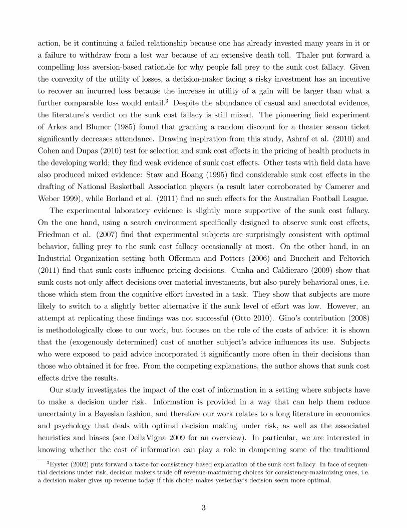
the world (Left and Right), for which probabilities are known: p � Pr(L). In the Decision blockp = 0:4.6 The payo¤s are determined by a state-dependent scoring function (see Figure 1).7

The parameterizations were chosen such that the loss domain was restricted while still providing

substantial incentives to perform Bayesian updating.

Figure 1: The scoring function. Note: the solid (dashed) line corresponds to the Decision (Identi�cation)block.

Subjects choose a number between 0 and 100 in steps of 0.5. If the state is L (R) the optimal

decision is 20 (80). Note that decisions below 20 and above 80 are strictly dominated. The

5A transcript of the instructions can be found in Appendix B.6We chose not to implement symmetric priors for a two reasons: �rst, the task could become trivial (Camerer

1987) or invite the usage of "obvious" (but possibly wrong) heuristics. Second, two scenarios with symmetric priorsmake the alignment of incentives and moves in the posterior across scenarios impossible to achieve (the urns wouldhave to be di¤erent, rendering moves in the posterior not comparable). This aspect is important because we wantto identify types in an environment (the Identi�cation block) that is as similar as possible to the Decision block.

7See Appendix A.1 for a detailed description of the choice environment and derivation of optimal decisionsaccording to the normative model. See Appendix D for a snapshot of the experiment (practice questions and maindecision screen).

6

information on the two state-dependent payo¤s is made available to subjects in three distinct

ways: on the screen (subjects can interactively learn the state-dependent payo¤s that result from

any particular value at all times), in graphical format and in table format (both in the paper

instructions). Our state-dependent payo¤ function is an adjusted quadratic scoring rule, which

was preferred to other proper scoring rules (e.g. O¤erman et al. 2009). The fundamental reason

behind our choice is the fact that many proper scoring rules do not provide a substantial incentive to

update beliefs unless radical moves in the posterior are observed. In other words, we need a scoring

rule function that is steep enough in the region where probability updating takes place. A common

problem with proper scoring rules is that risk attitudes may play a role in the observed choices.

However, this is not problematic in our setting as risk attitudes in�uence subjects�decisions in a

systematic fashion across treatments. Nonetheless, we statistically control for risk attitudes in our

analysis.

The information signal we provide to subjects is a lottery, for which we use an "urn" �lled

with balls. There are �ve balls in the urn, some black and some white. The distribution of balls is

itself state-dependent, but does not change across periods within a block and is visible to subjects

before every draw. In our design, drawing a ball from the urn is informative of the state of the

world, i.e. the probability of the realized state being L or R should be updated after drawing a

ball from the urn. In the Decision block, the urn contains one (three) black balls if the state is L

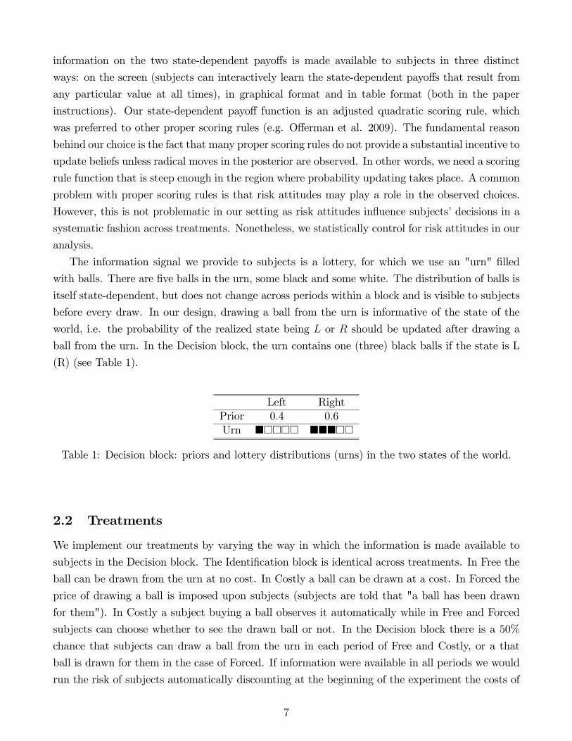
(R) (see Table 1).

Left RightPrior 0.4 0.6Urn ����� �����

Table 1: Decision block: priors and lottery distributions (urns) in the two states of the world.

2.2 Treatments

We implement our treatments by varying the way in which the information is made available to

subjects in the Decision block. The Identi�cation block is identical across treatments. In Free the

ball can be drawn from the urn at no cost. In Costly a ball can be drawn at a cost. In Forced the

price of drawing a ball is imposed upon subjects (subjects are told that "a ball has been drawn

for them"). In Costly a subject buying a ball observes it automatically while in Free and Forced

subjects can choose whether to see the drawn ball or not. In the Decision block there is a 50%

chance that subjects can draw a ball from the urn in each period of Free and Costly, or a that

ball is drawn for them in the case of Forced. If information were available in all periods we would

run the risk of subjects automatically discounting at the beginning of the experiment the costs of

7

information to be incurred, which would dissolve the psychological impact of an imposed cost. This

also forces subjects to experience decisions without information, which provides us with individual

decisions made without an information signal - a likely anchor for decisions when information is

made available. In the Costly and Forced treatments the information is priced at c = 0:3 tokens,

which is roughly 60% of the expected gain if expected utility maximization with Bayesian updating

is performed by a risk- and loss-neutral decision maker.

The Identi�cation block uses the same framework with a slightly di¤erent parameterization.

The idea is to create a decision environment that is equivalent in terms of incentives but that looks

su¢ ciently di¤erent for it not to be trivial nor invite the application of the decision rules employed

or learned in the Decision block. In particular, the ratio of the expected gain from using costly

information to the expected gain from not using information is similar across blocks (see Appendix

A.1 for details).

The Identi�cation block consists of three sequences of ten periods each. When available, infor-

mation is provided in every period. In the �rst sequence (I1), information is available for free. In

the second sequence (I2) information is available at a cost (c = 0:25 tokens, which is again roughly

60% of the expected gain). The �rst two sequences are akin to the Free and Costly treatments with

a 100% probability of getting information. In the third sequence subjects have to choose between

ten periods where they always have to pay for information (which is identical to Forced with a

100% probability of having information) and ten periods where information is never available. See

Figure 2 for a time-�ow diagram of the experiment.

Figure 2: Outline of the experimental design.

The Identi�cation block allows us to measure the value of information to subjects, i.e. how

their expected bene�ts compare to the costs they have to incur. We can distinguish between two

types of cost: monetary and cognitive. We present a classi�cation that takes both into account.

Accordingly, a subject buys information if:

Vi (Draw)� C1;i � C2 (�) � Vi (No Draw)

where � 2 fFree; Coslty;Forcedg, Vi (:) is the expected payo¤of a subject (which depends on many

8

cognitive factors like aptitude, mathematical training, con�dence, etc.), C1;i is the cognitive cost

of processing information, and C2 (:) is the monetary cost of information acquisition (equal to 0 in

I1 and equal to c in I2 and I3).8 In this sense, subjects incur C1 in I1 and C1+C2 in I2 in exchange

for information. In the Identi�cation block subjects make this choice in every period of I1 and I2.

In I3 subjects also choose whether they want to incur C1 + C2 or not, but their choice is binding

for ten periods. This stylized framework allows us to create an intuitive classi�cation of types.

A subject who chooses not to see information in I1 considers the cognitive cost of processing

it higher than the bene�ts. A subject who chooses not to buy information in I2 �nds the sum of

the cognitive and material costs of information higher than the bene�ts. Sequence I3 measures the

same relationship, but the choice is presented in a dichotomous way. The �rst two sequences not

only provide useful measurements in themselves, they also allow all subjects to experience what

it is like to use information for free and at a cost, especially considering that they faced di¤erent

treatment conditions in the Decision block.9 Combining data from sequences I1 and I3 allows us to

classify subjects in a way that improves our understanding of the major selection issues at hand.

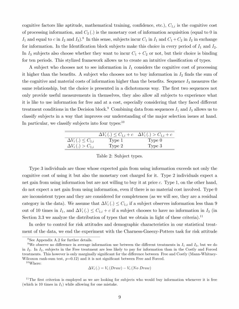
In particular, we classify subjects into four types:10

�Vi (:) � C1;i + c �Vi (:) > C1;i + c�Vi (:) � C1;i Type 1 Type 0�Vi (:) > C1;i Type 2 Type 3

Table 2: Subject types.

Type 3 individuals are those whose expected gain from using information exceeds not only the

cognitive cost of using it but also the monetary cost charged for it. Type 2 individuals expect a

net gain from using information but are not willing to buy it at price c. Type 1, on the other hand,

do not expect a net gain from using information, even if there is no material cost involved. Type 0

are inconsistent types and they are considered for completeness (as we will see, they are a residual

category in the data). We assume that �Vi (:) � C1;i if a subject observes information less than 9out of 10 times in I1, and �Vi (:) � C1;i + c if a subject chooses to have no information in I3 (inSection 3.3 we analyze the distribution of types that we obtain in light of these criteria).11

In order to control for risk attitudes and demographic characteristics in our statistical treat-

ment of the data, we end the experiment with the Charness-Gneezy-Potters task for risk attitude

8See Appendix A.2 for further details.9We observe no di¤erence in average information use between the di¤erent treatments in I1 and I3, but we do

in I2. In I2, subjects in the Free treatment are less likely to pay for information than in the Costly and Forcedtreatments. This however is only marginally signi�cant for the di¤erence between Free and Costly (Mann-Whitney-Wilcoxon rank-sum test, p=0.12) and it is not signi�cant between Free and Forced.10Where:

�Vi (:) = Vi (Draw)� Vi (No Draw)

11The �rst criterion is employed as we are looking for subjects who would buy information whenever it is free(which is 10 times in I1) while allowing for one mistake.

9

elicitation (Gneezy and Potters 1997, Charness and Gneezy 2010) and a questionnaire.12

3 Experimental Results

The experimental sessions were run at the CREED laboratory of the University of Amsterdam

between February and May 2012; they were programmed and conducted with the experiment

software z-Tree (Fischbacher 2007). A total of 166 subjects participated in 8 sessions, recruited

online from a subject pool of students at the University of Amsterdam. No subject participated

in more than one session. Fifty-�ve per cent of the participants were male and 57% were Business

or Economics majors. The typical session took 1 hour and 20 minutes with average earnings of 24

Euro (which includes a show-up fee of 7 Euro). Two of the sessions (47 participants, 22 in Free and

25 in Costly) had a di¤erent Identi�cation block.13 Unless mentioned otherwise, all data discussed

in this section pertains to decision making in the Decision block. Sub-section 3.1 describes the

data. Sub-section 3.2 analyzes the di¤erence in decision making across treatments. Sub-section

3.3 expands the analysis by including subject type data.

3.1 Data Description

Table 3 provides a summary of descriptive statistics for the collected data. Di¤erences in individual

traits are not statistically signi�cant across treatments. Average period payo¤ is signi�cantly

higher in the Free treatment than in the Forced treatment. This is to be expected as subjects

incur no costs in the Free treatment as opposed to the Costly and Forced treatments. Percentage

of information seen refers to the fraction of times subjects choose to observe information when it is

available. Naturally, when information is costly and optional, fewer subjects choose to observe it.

The Costly treatment thus shows signi�cantly fewer information views than the Free and Forced

treatments. We observe that subjects choose not to see information (draw a ball) sometimes, even

when it is free or already paid for. This is possible as in all treatments we let subjects have the

option of not drawing a ball, reasoning in terms of the stylized model discussed in Section 2.2.

That is, some subjects, denoted as Type 0 and Type 1, �nd the cognitive costs of using information

higher than the bene�ts. Additionally, many subjects experiment with drawing and not drawing

a ball and thus do not observe information in some of the periods.14

12The risk attitute elicitation task consists in asking subjects how they wish to allocate an endowment of threetokens between a safe account and an account that multiplies the invested amount by a factor of 2.5 with 50%probability and destroys the money with 50% probability. The questionnaire asked whether subjects had had Mathin high school, how many Math courses they had completed at university, their gender, age, and major.13The Decision Block was identical across all sessions. The Identi�cation Block was changed after the �rst two

sessions in order to enhance the validity of the type classi�cation. For this reason no data from these two sessionsis used in analyses containing type variables.14Ignoring type 0 and 1 subjects, % information seen changes to 92% in the Free treatment and 87% in the Forced

treatment. Of all subjects, only 6% in Free and 11% in Forced chose never to draw a ball (this �gure is 21% inCostly).

10

Free Costly ForcedN 65 65 36Risk 2:06 1:93 2:10

Math courses 2:38 2:95 2:55% Female 37% 48% 44%

Average period payo¤ 3:10 3:00 2:84% Information seen 79% 56% 74%

Table 3: Summary statistics

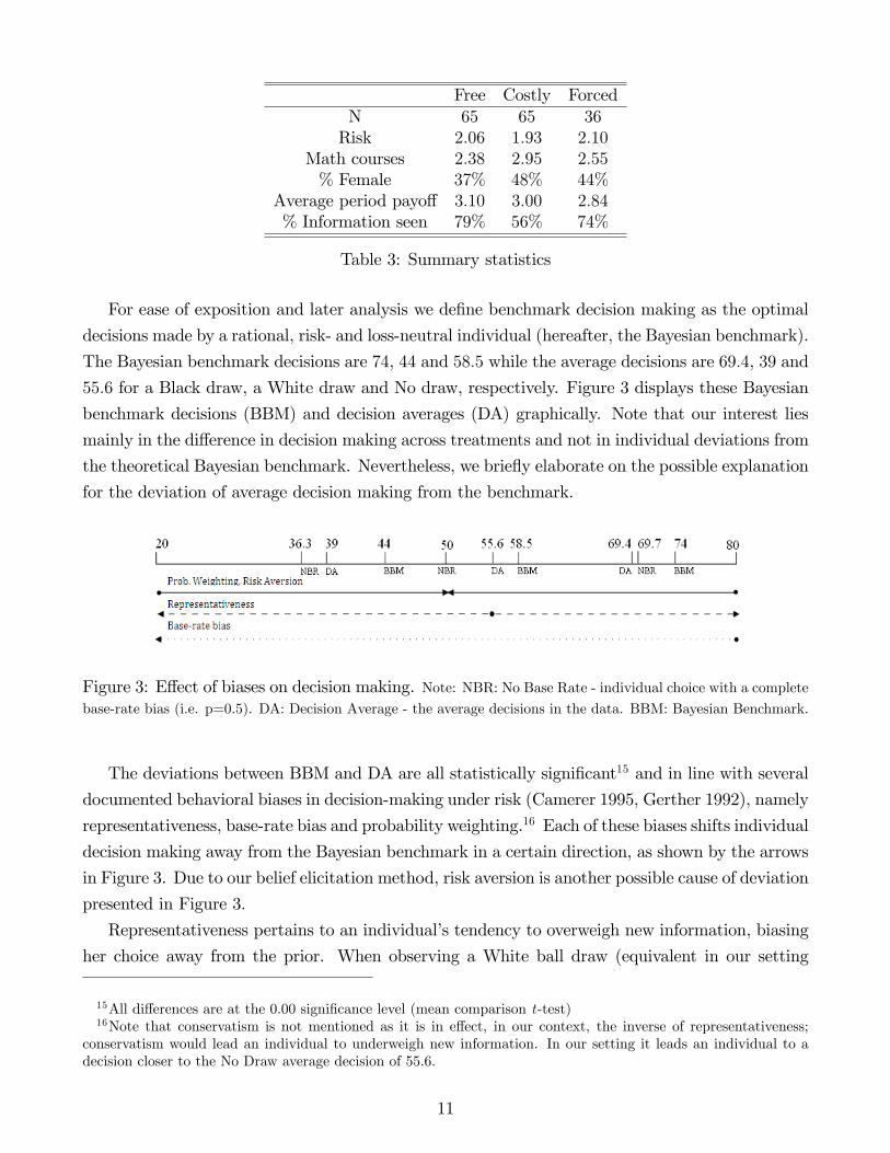
For ease of exposition and later analysis we de�ne benchmark decision making as the optimal

decisions made by a rational, risk- and loss-neutral individual (hereafter, the Bayesian benchmark).

The Bayesian benchmark decisions are 74, 44 and 58:5 while the average decisions are 69:4, 39 and

55:6 for a Black draw, a White draw and No draw, respectively. Figure 3 displays these Bayesian

benchmark decisions (BBM) and decision averages (DA) graphically. Note that our interest lies

mainly in the di¤erence in decision making across treatments and not in individual deviations from

the theoretical Bayesian benchmark. Nevertheless, we brie�y elaborate on the possible explanation

for the deviation of average decision making from the benchmark.

Figure 3: E¤ect of biases on decision making. Note: NBR: No Base Rate - individual choice with a completebase-rate bias (i.e. p=0.5). DA: Decision Average - the average decisions in the data. BBM: Bayesian Benchmark.

The deviations between BBM and DA are all statistically signi�cant15 and in line with several

documented behavioral biases in decision-making under risk (Camerer 1995, Gerther 1992), namely

representativeness, base-rate bias and probability weighting.16 Each of these biases shifts individual

decision making away from the Bayesian benchmark in a certain direction, as shown by the arrows

in Figure 3. Due to our belief elicitation method, risk aversion is another possible cause of deviation

presented in Figure 3.

Representativeness pertains to an individual�s tendency to overweigh new information, biasing

her choice away from the prior. When observing a White ball draw (equivalent in our setting

15All di¤erences are at the 0.00 signi�cance level (mean comparison t-test)16Note that conservatism is not mentioned as it is in e¤ect, in our context, the inverse of representativeness;

conservatism would lead an individual to underweigh new information. In our setting it leads an individual to adecision closer to the No Draw average decision of 55:6.

11

to receiving new information), this bias leads an individual to overweigh the likelihood this ball

draw signals that the state of the world is Left. A similar overweighting of the Right state of

the world occurs if the ball is Black. Representativeness thus results in decisions which are closer

to the extremes of 20 and 80 than the benchmark decision. The base-rate bias pertains to the

tendency of an individual to underweigh the prior when receiving new information. That is, to

update her belief as if the prior is closer to 0:5 than it actually is. Note that this is not the

same as representativeness. Since the prior in our design indicates that Left is less likely than

Right, this bias brings subjects to over-update the probability of Left after any ball draw. In case

an individual exhibits base rate bias she thus deviates towards 20 after a ball draw. Probability

weighting describes a tendency of individuals to overweigh low probabilities and underweigh high

probabilities (Holt and Smith 2009). In our design, this results in a deviation towards 50 after

both a Black and White ball draw. A risk averse individual shifts her decision towards less risky

options, which is translated in our design to a deviation towards 50. Such a deviation insures

a lower gap in the state dependent payo¤ than in the benchmark decision. Risk aversion and

probability weighting are the only two e¤ects that can in�uence decisions without a ball draw.

Both of them can explain the deviation in average decision making with no additional information.

As no single bias can explain the deviation after a White draw and a Black draw, only some

combination of the discussed biases, and risk aversion, can explain the pattern observed in our

data.

3.2 Treatment e¤ects

We now begin with an analysis of the aggregate treatment outcomes. Figure 4 presents �ve-period

average decisions over the duration of the Decision block by treatment and information condition

(Black draw, No draw and White draw). Decision averages visibly di¤er across treatments and

in all periods after a ball draw. No such di¤erence is discernible after No draw. Table 4 shows

the aggregate treatment averages by information condition and treatment. After both a White

draw and a Black draw there are signi�cant di¤erences between the Costly and Free treatments

(two-sided Mann-Whitney-Wilcoxon rank-sum test, MWW hereafter: p = 0:02 and p = 0:01,

respectively), and between the Forced and Free treatments (MWW: p = 0:04 and p = 0:01,

respectively). No signi�cant di¤erences are found between the Costly and Forced treatments.

Without a draw from the urn there are no signi�cant di¤erences between any of the treatments.

The shift in average decision making between both the Costly and Forced treatments and the Free

treatment is thus signi�cant only after a ball draw. It is an upward shift after a Black draw and

downward one following a White draw.

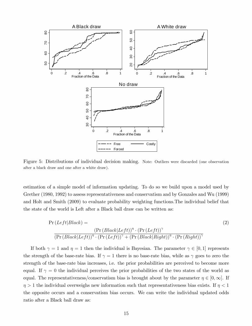
Figure 5 presents the cumulative distribution functions of individual decision by information

condition. We de�ne indiviual decision di�t as the decision of subject i in period t and in information

condition � 2 fBlack;White;No Infog. Average decision �di� is de�ned as the average of subject

12

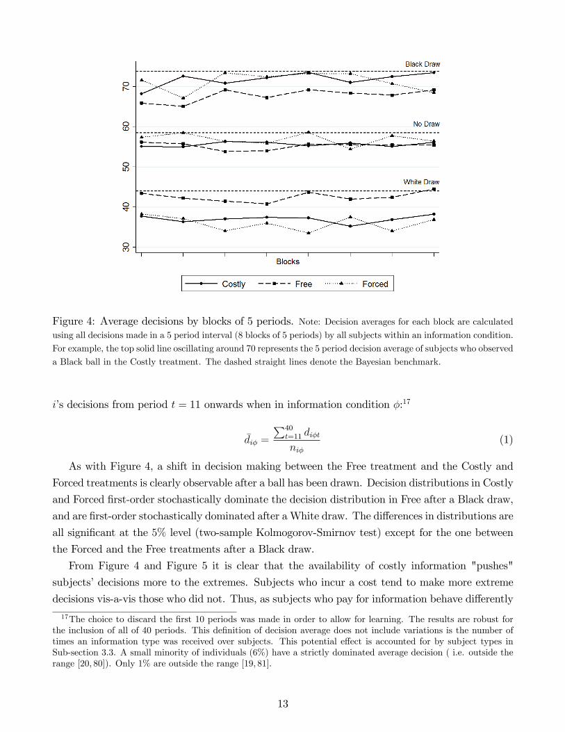
Figure 4: Average decisions by blocks of 5 periods. Note: Decision averages for each block are calculatedusing all decisions made in a 5 period interval (8 blocks of 5 periods) by all subjects within an information condition.

For example, the top solid line oscillating around 70 represents the 5 period decision average of subjects who observed

a Black ball in the Costly treatment. The dashed straight lines denote the Bayesian benchmark.

i�s decisions from period t = 11 onwards when in information condition �:17

�di� =

P40t=11 di�tni�

(1)

As with Figure 4, a shift in decision making between the Free treatment and the Costly and

Forced treatments is clearly observable after a ball has been drawn. Decision distributions in Costly

and Forced �rst-order stochastically dominate the decision distribution in Free after a Black draw,

and are �rst-order stochastically dominated after a White draw. The di¤erences in distributions are

all signi�cant at the 5% level (two-sample Kolmogorov-Smirnov test) except for the one between

the Forced and the Free treatments after a Black draw.

From Figure 4 and Figure 5 it is clear that the availability of costly information "pushes"

subjects�decisions more to the extremes. Subjects who incur a cost tend to make more extreme

decisions vis-a-vis those who did not. Thus, as subjects who pay for information behave di¤erently

17The choice to discard the �rst 10 periods was made in order to allow for learning. The results are robust forthe inclusion of all of 40 periods. This de�nition of decision average does not include variations is the number oftimes an information type was received over subjects. This potential e¤ect is accounted for by subject types inSub-section 3.3. A small minority of individuals (6%) have a strictly dominated average decision ( i.e. outside therange [20; 80]). Only 1% are outside the range [19; 81].

13

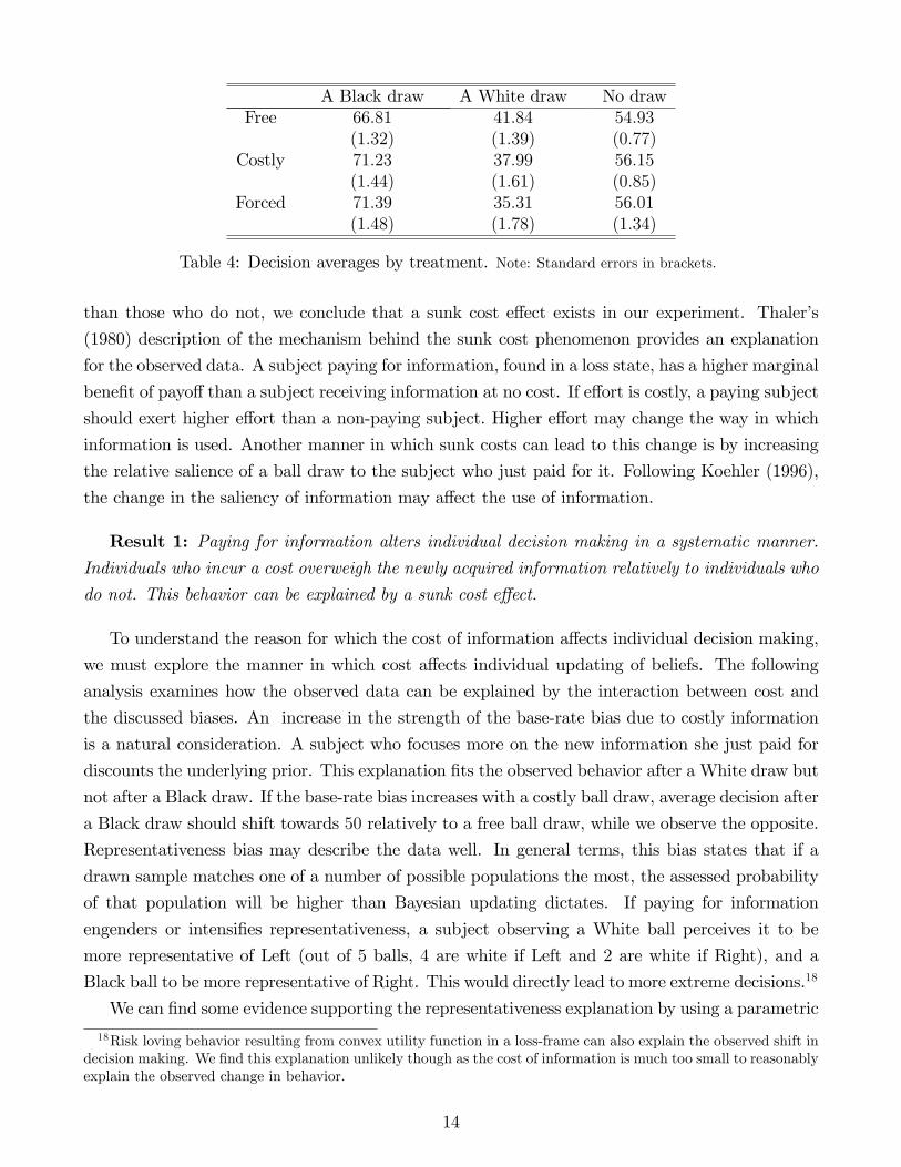
A Black draw A White draw No drawFree 66:81 41:84 54:93

(1:32) (1:39) (0:77)Costly 71:23 37:99 56:15

(1:44) (1:61) (0:85)Forced 71:39 35:31 56:01

(1:48) (1:78) (1:34)

Table 4: Decision averages by treatment. Note: Standard errors in brackets.

than those who do not, we conclude that a sunk cost e¤ect exists in our experiment. Thaler�s

(1980) description of the mechanism behind the sunk cost phenomenon provides an explanation

for the observed data. A subject paying for information, found in a loss state, has a higher marginal

bene�t of payo¤ than a subject receiving information at no cost. If e¤ort is costly, a paying subject

should exert higher e¤ort than a non-paying subject. Higher e¤ort may change the way in which

information is used. Another manner in which sunk costs can lead to this change is by increasing

the relative salience of a ball draw to the subject who just paid for it. Following Koehler (1996),

the change in the saliency of information may a¤ect the use of information.

Result 1: Paying for information alters individual decision making in a systematic manner.Individuals who incur a cost overweigh the newly acquired information relatively to individuals who

do not. This behavior can be explained by a sunk cost e¤ect.

To understand the reason for which the cost of information a¤ects individual decision making,

we must explore the manner in which cost a¤ects individual updating of beliefs. The following

analysis examines how the observed data can be explained by the interaction between cost and

the discussed biases. An increase in the strength of the base-rate bias due to costly information

is a natural consideration. A subject who focuses more on the new information she just paid for

discounts the underlying prior. This explanation �ts the observed behavior after a White draw but

not after a Black draw. If the base-rate bias increases with a costly ball draw, average decision after

a Black draw should shift towards 50 relatively to a free ball draw, while we observe the opposite.

Representativeness bias may describe the data well. In general terms, this bias states that if a

drawn sample matches one of a number of possible populations the most, the assessed probability

of that population will be higher than Bayesian updating dictates. If paying for information

engenders or intensi�es representativeness, a subject observing a White ball perceives it to be

more representative of Left (out of 5 balls, 4 are white if Left and 2 are white if Right), and a

Black ball to be more representative of Right. This would directly lead to more extreme decisions.18

We can �nd some evidence supporting the representativeness explanation by using a parametric

18Risk loving behavior resulting from convex utility function in a loss-frame can also explain the observed shift indecision making. We �nd this explanation unlikely though as the cost of information is much too small to reasonablyexplain the observed change in behavior.

14

Free CostlyForced

3040

5060

7080

0 .2 .4 .6 .8 1Fraction of the Data

No draw

5060

7080

0 .2 .4 .6 .8 1Fraction of the Data

A Black draw

2030

4050

60

0 .2 .4 .6 .8 1Fraction of the Data

A White draw

Figure 5: Distributions of individual decision making. Note: Outliers were discarded (one observationafter a black draw and one after a white draw).

estimation of a simple model of information updating. To do so we build upon a model used by

Grether (1980, 1992) to assess representativeness and conservatism and by Gonzales andWu (1999)

and Holt and Smith (2009) to evaluate probability weighting functions.The individual belief that

the state of the world is Left after a Black ball draw can be written as:

Pr (LeftjBlack) = (2)

(Pr (BlackjLeft))� � (Pr (Left))

(Pr (BlackjLeft))� � (Pr (Left)) + (Pr (BlackjRight))� � (Pr (Right))

If both = 1 and � = 1 then the individual is Bayesian. The parameter 2 [0; 1] representsthe strength of the base-rate bias. If = 1 there is no base-rate bias, while as goes to zero the

strength of the base-rate bias increases, i.e. the prior probabilities are perceived to become more

equal. If = 0 the individual perceives the prior probabilities of the two states of the world as

equal. The representativeness/conservatism bias is brought about by the parameter � 2 [0;1]. If� > 1 the individual overweighs new information such that representativeness bias exists. If � < 1

the opposite occurs and a conservatism bias occurs. We can write the individual updated odds

ratio after a Black ball draw as:

15

Pr (LeftjBlack)Pr (RightjBlack) =

�Pr (BlackjLeft)Pr (BlackjRight)

����Pr (Left)

Pr (Right)

� (3)

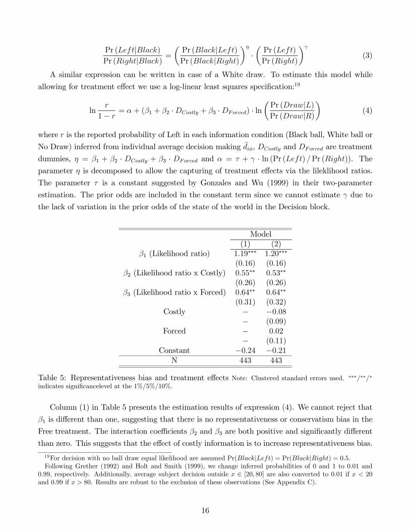
A similar expression can be written in case of a White draw. To estimate this model while

allowing for treatment e¤ect we use a log-linear least squares speci�cation:19

lnr

1� r = �+ (�1 + �2 �DCostly + �3 �DForced) � ln�Pr (DrawjL)Pr (DrawjR)

�(4)

where r is the reported probability of Left in each information condition (Black ball, White ball or

No Draw) inferred from individual average decision making �di�, DCostly and DForced are treatment

dummies, � = �1 + �2 � DCostly + �3 � DForced and � = � + � ln (Pr (Left) =Pr (Right)). Theparameter � is decomposed to allow the capturing of treatment e¤ects via the lileklihood ratios.

The parameter � is a constant suggested by Gonzales and Wu (1999) in their two-parameter

estimation. The prior odds are included in the constant term since we cannot estimate due to

the lack of variation in the prior odds of the state of the world in the Decision block.

Model(1) (2)

�1 (Likelihood ratio) 1:19��� 1:20���

(0:16) (0:16)�2 (Likelihood ratio x Costly) 0:55�� 0:53��

(0:26) (0:26)�3 (Likelihood ratio x Forced) 0:64�� 0:64��

(0:31) (0:32)Costly � �0:08

� (0:09)Forced � 0:02

� (0:11)Constant �0:24 �0:21

N 443 443

Table 5: Representativeness bias and treatment e¤ects Note: Clustered standard errors used. ���=��=�

indicates signi�cancelevel at the 1%=5%=10%.

Column (1) in Table 5 presents the estimation results of expression (4). We cannot reject that

�1 is di¤erent than one, suggesting that there is no representativeness or conservatism bias in the

Free treatment. The interaction coe¢ cients �2 and �3 are both positive and signi�cantly di¤erent

than zero. This suggests that the e¤ect of costly information is to increase representativeness bias.

19For decision with no ball draw equal likelihood are assumed Pr(BlackjLeft) = Pr(BlackjRight) = 0:5.Following Grether (1992) and Holt and Smith (1999), we change inferred probabilities of 0 and 1 to 0:01 and

0:99, respectively. Additionally, average subject decision outside x 2 [20; 80] are also converted to 0:01 if x < 20and 0:99 if x > 80. Results are robust to the exclusion of these observations (See Appendix C).

16

Column (2) presents an estimation with independent treatment dummy variables.20 This allows for

the possibility of the Costly and Forced treatment to have an e¤ect on individual decisions through

channels other than representativeness (i.e. through the constant � or the scope of the base rate

bias ). We do not �nd a signi�cant e¤ect of treatment dummies on reported probability odds. Our

estimation results support the preceding qualitative discussion on the possible channels through

which sunk costs a¤ect individual decision making. An intensi�cation of representativeness bias

following costly information is the most likely explanation of our results.

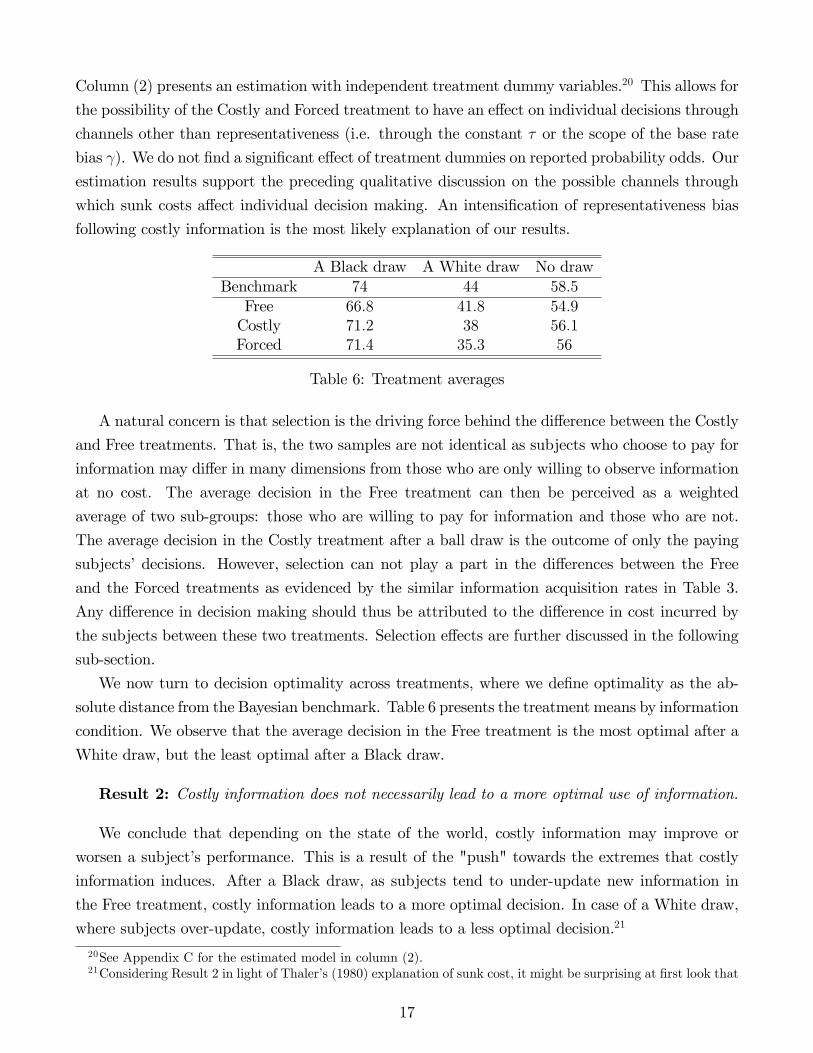
A Black draw A White draw No drawBenchmark 74 44 58:5

Free 66:8 41:8 54:9Costly 71:2 38 56:1Forced 71:4 35:3 56

Table 6: Treatment averages

A natural concern is that selection is the driving force behind the di¤erence between the Costly

and Free treatments. That is, the two samples are not identical as subjects who choose to pay for

information may di¤er in many dimensions from those who are only willing to observe information

at no cost. The average decision in the Free treatment can then be perceived as a weighted

average of two sub-groups: those who are willing to pay for information and those who are not.

The average decision in the Costly treatment after a ball draw is the outcome of only the paying

subjects�decisions. However, selection can not play a part in the di¤erences between the Free

and the Forced treatments as evidenced by the similar information acquisition rates in Table 3.

Any di¤erence in decision making should thus be attributed to the di¤erence in cost incurred by

the subjects between these two treatments. Selection e¤ects are further discussed in the following

sub-section.

We now turn to decision optimality across treatments, where we de�ne optimality as the ab-

solute distance from the Bayesian benchmark. Table 6 presents the treatment means by information

condition. We observe that the average decision in the Free treatment is the most optimal after a

White draw, but the least optimal after a Black draw.

Result 2: Costly information does not necessarily lead to a more optimal use of information.

We conclude that depending on the state of the world, costly information may improve or

worsen a subject�s performance. This is a result of the "push" towards the extremes that costly

information induces. After a Black draw, as subjects tend to under-update new information in

the Free treatment, costly information leads to a more optimal decision. In case of a White draw,

where subjects over-update, costly information leads to a less optimal decision.21

20See Appendix C for the estimated model in column (2).21Considering Result 2 in light of Thaler�s (1980) explanation of sunk cost, it might be surprising at �rst look that

17

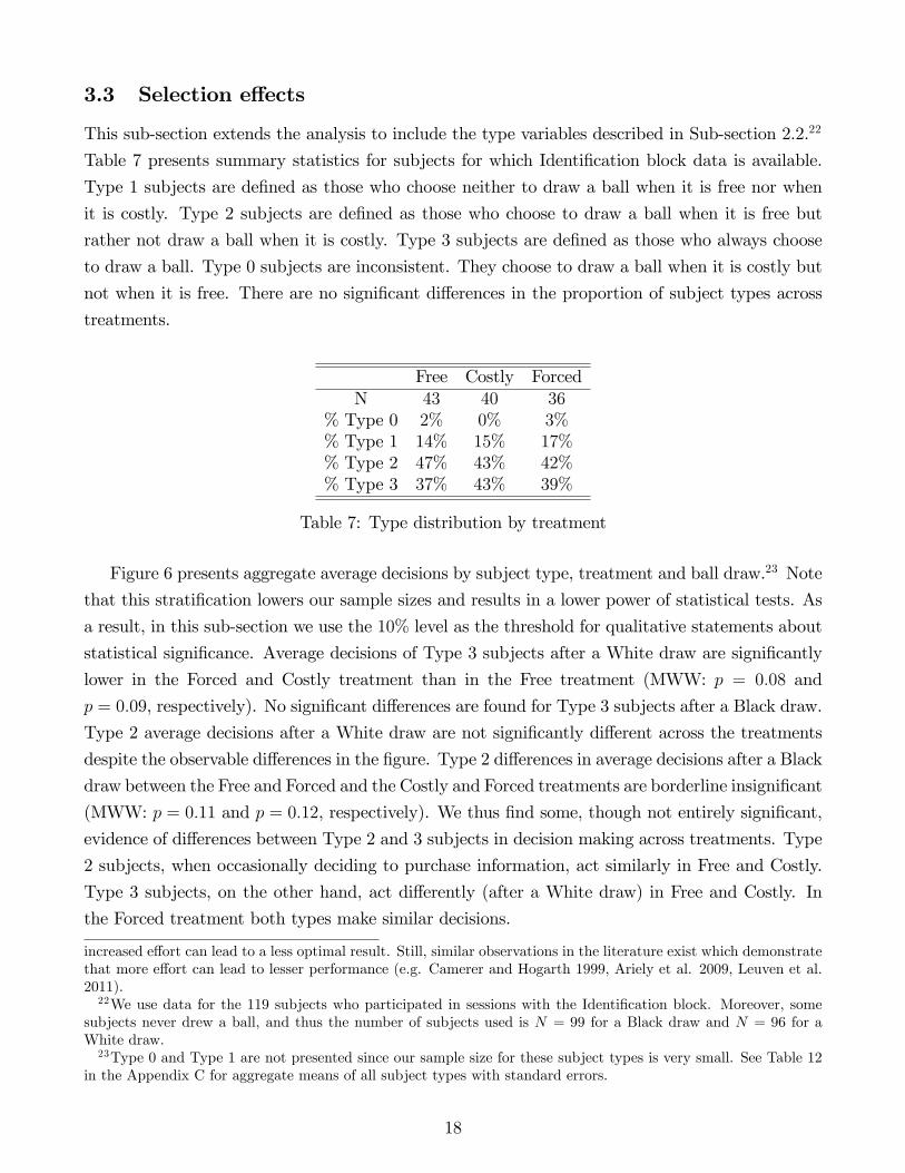
3.3 Selection e¤ects

This sub-section extends the analysis to include the type variables described in Sub-section 2.2.22

Table 7 presents summary statistics for subjects for which Identi�cation block data is available.

Type 1 subjects are de�ned as those who choose neither to draw a ball when it is free nor when

it is costly. Type 2 subjects are de�ned as those who choose to draw a ball when it is free but

rather not draw a ball when it is costly. Type 3 subjects are de�ned as those who always choose

to draw a ball. Type 0 subjects are inconsistent. They choose to draw a ball when it is costly but

not when it is free. There are no signi�cant di¤erences in the proportion of subject types across

treatments.

Free Costly ForcedN 43 40 36

% Type 0 2% 0% 3%% Type 1 14% 15% 17%% Type 2 47% 43% 42%% Type 3 37% 43% 39%

Table 7: Type distribution by treatment

Figure 6 presents aggregate average decisions by subject type, treatment and ball draw.23 Note

that this strati�cation lowers our sample sizes and results in a lower power of statistical tests. As

a result, in this sub-section we use the 10% level as the threshold for qualitative statements about

statistical signi�cance. Average decisions of Type 3 subjects after a White draw are signi�cantly

lower in the Forced and Costly treatment than in the Free treatment (MWW: p = 0:08 and

p = 0:09, respectively). No signi�cant di¤erences are found for Type 3 subjects after a Black draw.

Type 2 average decisions after a White draw are not signi�cantly di¤erent across the treatments

despite the observable di¤erences in the �gure. Type 2 di¤erences in average decisions after a Black

draw between the Free and Forced and the Costly and Forced treatments are borderline insigni�cant

(MWW: p = 0:11 and p = 0:12, respectively). We thus �nd some, though not entirely signi�cant,

evidence of di¤erences between Type 2 and 3 subjects in decision making across treatments. Type

2 subjects, when occasionally deciding to purchase information, act similarly in Free and Costly.

Type 3 subjects, on the other hand, act di¤erently (after a White draw) in Free and Costly. In

the Forced treatment both types make similar decisions.

increased e¤ort can lead to a less optimal result. Still, similar observations in the literature exist which demonstratethat more e¤ort can lead to lesser performance (e.g. Camerer and Hogarth 1999, Ariely et al. 2009, Leuven et al.2011).22We use data for the 119 subjects who participated in sessions with the Identi�cation block. Moreover, some

subjects never drew a ball, and thus the number of subjects used is N = 99 for a Black draw and N = 96 for aWhite draw.23Type 0 and Type 1 are not presented since our sample size for these subject types is very small. See Table 12

in the Appendix C for aggregate means of all subject types with standard errors.

18

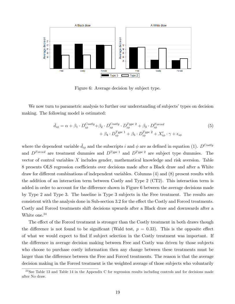
Figure 6: Average decision by subject type.

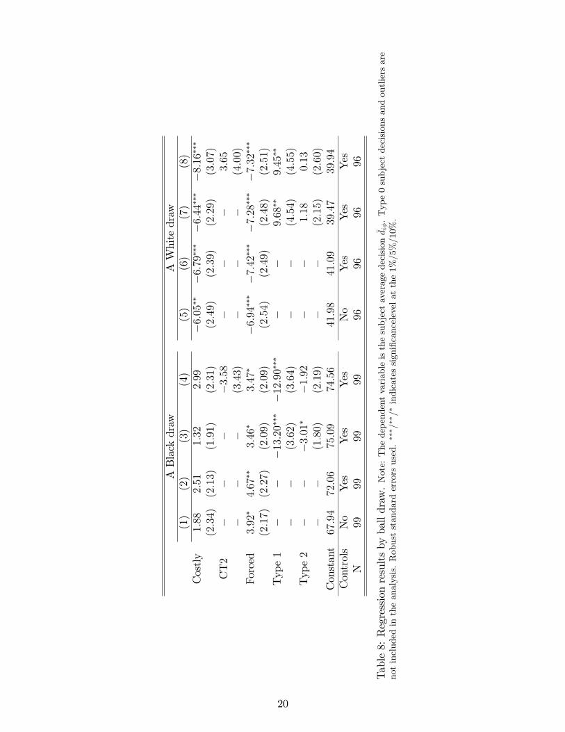
We now turn to parametric analysis to further our understanding of subjects�types on decision

making. The following model is estimated:

�di� = �+ �1 �DCostlyi� +�2 �DCostly

i� �DType 2i� + �3 �DForced

i� (5)

+ �4 �DType 1i� + �5 �DType 2

i� +X 0i� � + �i�

where the dependent variable �di� and the subscripts i and � are as de�ned in equation (1). DCostly

and DForced are treatment dummies and DType 1 and DType 2 are subject type dummies. The

vector of control variables X includes gender, mathematical knowledge and risk aversion. Table

8 presents OLS regression coe¢ cients over decisions made after a Black draw and after a White

draw for di¤erent combinations of independent variables. Columns (4) and (8) present results with

the addition of an interaction term between Costly and Type 2 (CT2). This interaction term is

added in order to account for the di¤erence shown in Figure 6 between the average decisions made

by Type 2 and Type 3. The baseline is Type 3 subjects in the Free treatment. The results are

consistent with the analysis done in Sub-section 3.2 for the e¤ect the Costly and Forced treatments.

Costly and Forced treatments shift decisions upwards after a Black draw and downwards after a

White one.24

The e¤ect of the Forced treatment is stronger than the Costly treatment in both draws though

the di¤erence is not found to be signi�cant (Wald test, p = 0:33). This is the opposite e¤ect

of what we would expect to �nd if subject selection in the Costly treatment was important. If

the di¤erence in average decision making between Free and Costly was driven by those subjects

who choose to purchase costly information then any change between these treatments must be

larger than the di¤erence between the Free and Forced treatments. The reason is that the average

decision making in the Forced treatment is the weighted average of those subjects who voluntarily

24See Table 13 and Table 14 in the Appendix C for regression results including controls and for decisions madeafter No draw.

19

ABlackdraw

AWhitedraw

(1)

(2)

(3)

(4)

(5)

(6)

(7)

(8)

Costly

1:88

2:51

1:32

2:99

�6:05��

�6:79����6:44����8:16���

(2:34)

(2:13)

(1:91)

(2:31)

(2:49)

(2:39)

(2:29)

(3:07)

CT2

��

��3:58

��

�3:65

��

�(3:43)

��

�(4:00)

Forced

3:92�

4:67��

3:46�

3:47�

�6:94����7:42����7:28����7:32���

(2:17)

(2:27)

(2:09)

(2:09)

(2:54)

(2:49)

(2:48)

(2:51)

Type1

��

�13:20���

�12:90���

��

9:68��

9:45��

��

(3:62)

(3:64)

��

(4:54)

(4:55)

Type2

��

�3:01�

�1:92

��

1:18

0:13

��

(1:80)

(2:19)

��

(2:15)

(2:60)

Constant

67:94

72:06

75:09

74:56

41:98

41:09

39:47

39:94

Controls

No

Yes

Yes

Yes

No

Yes

Yes

Yes

N99

9999

9996

9696

96

Table8:Regressionresultsbyballdraw.Note:Thedependentvariableisthesubjectaveragedecision

� di�.Type0subjectdecisionsandoutliersare

notincludedintheanalysis.Robuststandarderrorsused.��� =��=�indicatessigni�cancelevelatthe1%=5%=10%.

20

buy costly information and those who do not. It is thus the cost of information itself that directly

a¤ects subject behavior.

Result 3: Observed di¤erences are not driven by selection.

Using Figure 6, we can attempt to explain why a stronger deviation is observed in Forced than

in Costly. To do so, we focus our attention on the behavior of Type 2 subjects.25 Type 2 subjects�

average decision after both a Black and a White draw are similar in the Free and Costly treatments

and only shift in the Forced treatment. This is consistent with our type dichotomy if we consider

Type 2 subjects�behavior in the Costly treatment as an exploratory one, investigating the bene�ts

and costs of opting for a ball draw. Such "testing of the waters" may be less a¤ected by the cost

of drawing a ball. Average decisions for Type 2 and Type 3 subjects should then be equal in Free

and Forced while being di¤erent in Costly. This is indeed the case after a White draw but not

entirely after a Black draw.26 The weak e¤ect of Costly in Table 8 is thus the average e¤ect of

Type 2 and Type 3 subjects. This also explains the weakly signi�cant e¤ect of the Type 2 dummy

seen in Table 8. When adding the interaction term CT2 the shift in decision making after both

Costly and Forced becomes highly similar. Additionally, after a Black draw, the Type 2 dummy

coe¢ cient is no longer signi�cant. Table 8 also exhibits signi�cant di¤erences between Type 3 and

Type 1 subjects�performance. Using a Wald test we also �nd signi�cant di¤erences between Type

2 and Type 1 subjects (p-values: 0:09 after a White draw and 0:01 after a Black draw).

Result 4: Subjects who use freely available information (Type 2 and Type 3 subjects) performsimilarly in the Free and Forced treatments and di¤erently from subjects who do not (Type 1). Type

1 subjects substantially under-weigh new information.

The experimental results discussed in Sub-section 3.2 and Sub-section 3.3 are closely related.

We show that the variance in the cost of information is the driver of our result using both the

Forced treatment and by using the subject type data. We are thus able to evaluate the e¤ect that

subject heterogeneity, with respect to information purchasing decisions, has on our results. The

change in behavior due to the cost of information is signi�cant and systematic. Sunk cost e¤ects

are thus shown to have an e¤ect on decision making in our experimental setting.

4 Pricing Information

In general, reliable and useful information is a lever towards better results. Our choice framework

presents subjects with the opportunity of increasing expected gains through the incorporation

25Remember that though we de�ne Type 2 subjects as those who are willing to draw a ball only at no cost, westill observe those subjects drawing a ball in the Costly treatment occasionally.26After a Black draw Type 3 subjects average decision is signi�cantly higher than Type 2 subjects in the Free

treatment (MWW: p = 0:07).

21

of new information. In Sub-section 3.2 we observed that subjects put relatively more weight on

information they had to pay for, but this does not always lead to better decisions. However, even

if information always pushed subjects closer to the optimum, this would tell us little about the

e¢ ciency of using information. In other words, the gains realized from using information (because

of higher-payo¤ choices due to reduced uncertainty) might not compensate the cost paid for it.27

In this section we investigate this implicit trade-o¤ using a small exercise that demonstrates how

information should be priced (or subsidized) in order for it to be pro�table for subjects. Hence, in

this section we move our focus away from the e¤ect of sunk costs to the e¢ ciency gains obtained

from using information.

To answer this question we compute the cost levels that would make subjects indi¤erent between

paying for information and having no information. We use data from the Decision block in this

analysis, and only from the Free and Forced treatments (the selection present in Costly complicates

data interpretation as many subjects chose never to observe information - cf. Sub-section 3.1). We

want to calculate the individual cost level ci that makes the following equality hold:X�2fBlack;Whiteg

Pr (�)V��di��� ci = V

��di;No Draw

�where V (�) is the payo¤ that would result from implementing the average decision �di;� (as de�nedin equation 1) of each subject in the respective information condition.

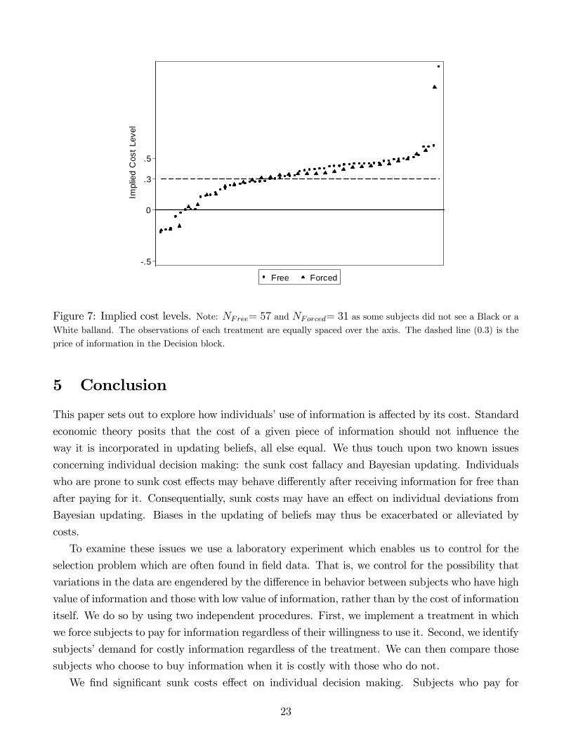
Figure 7 presents a plot of the implied individual cost levels in ascending order. To be more

precise, ci is the cost level which would make subject i indi¤erent between facing one decision with

paid information and one decision without information. This value is conditional on i�s average

decisions in each information condition. We observe that the great majority of subjects should be

willing to pay for information (ci � 0): only 10% would have to be subsidized (ci < 0). Moreover,

60% of our subjects have an implied cost level above 0:3, which means that information was priced

in a bene�cial way for the majority of them. A noteworthy aspect is the fact that Forced did not

lead to a better overall use of information, as the distribution of ci in this treatment follows the

one in Free quite closely. The reason is that, as mentioned, subjects in Forced got very close to

the optimum in case of a Black ball but overshot in case of a White ball (see Figure 4).

The main message from this exercise is that information pricing is far from trivial from a policy

perspective due to the underlying trade-o¤. On the one hand, it can provide (the right) incentives if

it leads to a better incorporation of information in decision making. On the other hand, individuals

might end up worse o¤ if the price paid for information cancels the bene�ts derived from reducing

uncertainty.

27Recall that we priced information at roughly 60% of the expected gain of the Bayesian benchmark.

22

­.5

0

.3

.5

Impl

ied 

Cos

t Lev

el

Free Forced

Figure 7: Implied cost levels. Note: NFree= 57 and NForced= 31 as some subjects did not see a Black or aWhite balland. The observations of each treatment are equally spaced over the axis. The dashed line (0.3) is the

price of information in the Decision block.

5 Conclusion

This paper sets out to explore how individuals�use of information is a¤ected by its cost. Standard

economic theory posits that the cost of a given piece of information should not in�uence the

way it is incorporated in updating beliefs, all else equal. We thus touch upon two known issues

concerning individual decision making: the sunk cost fallacy and Bayesian updating. Individuals

who are prone to sunk cost e¤ects may behave di¤erently after receiving information for free than

after paying for it. Consequentially, sunk costs may have an e¤ect on individual deviations from

Bayesian updating. Biases in the updating of beliefs may thus be exacerbated or alleviated by

costs.

To examine these issues we use a laboratory experiment which enables us to control for the

selection problem which are often found in �eld data. That is, we control for the possibility that

variations in the data are engendered by the di¤erence in behavior between subjects who have high

value of information and those with low value of information, rather than by the cost of information

itself. We do so by using two independent procedures. First, we implement a treatment in which

we force subjects to pay for information regardless of their willingness to use it. Second, we identify

subjects�demand for costly information regardless of the treatment. We can then compare those

subjects who choose to buy information when it is costly with those who do not.

We �nd signi�cant sunk costs e¤ect on individual decision making. Subjects who pay for

23

information put higher weight on it relative to subjects who receive identical information at no cost.

This e¤ect leads to a shift of updated beliefs towards the extremes. Decision making with costly

information can be closer to or further from the correct Bayesian updating compared to decision

making with free information. If subjects under-update their beliefs using free information, then

costly information "pushes" their decision closer to the optimum. In case the opposite occurs, i.e.

subjects over-update with free information, then costly information "pushes" them further away

from the optimal outcome.

Since placing a cost on information can be bene�cial or harmful, this paper suggests that policy

makers should consider the implications of providing costly information. This can be favorable

as long as individuals under-update new information when it is provided freely. The downside

of making information costly is that a trade-o¤ exists between more optimal behavior and lower

demand for information. To circumvent lower demand a policy maker can force a cost via a

mandatory fee or tax on information. This fee must be directly related to the information such

that an individual does not internalize the fee in advance, thus ignoring its association to the

provided information. Our results may be of importance for experimental research on the value

of information. Economists sometimes vary the cost of information across treatments in order to

elicit subjects�value of information. Our paper shows that the cost of information itself can a¤ect

decision making.

Having shown the existence of sunk cost e¤ects on the use of information, further examination

may be of interest. A natural extension of this paper is to add treatments with di¤ering information

costs. For example, if lower costs are found to induce changes in behavior similar to the ones

found in this paper, then using costly information may be useful also in cases where demand for

information is sensitive to price.

24

References

Ariely, Dan, Uri Gneezy, George Loewenstein, and Nina Mazar (2009). Large stakes and big

mistakes. Review of Economic Studies 76 (2), 451 �469.

Arkes, Hal R and Catherine Blumer (1985). The psychology of sunk cost. Organizational Be-

havior and Human Decision Processes 35 (1), 124 �140.

Ashraf, Nava, James Berry, and Jesse M. Shapiro (2010). Can higher prices stimulate product

use? evidence from a �eld experiment in zambia. American Economic Review 100 (5), 2383�

2413.

Borland, Je¤, Leng Lee, and Robert D. Macdonald (2011). Escalation e¤ects and the player

draft in the a�. Labour Economics 18 (3), 371 �380.

Camerer, Colin (1995). Individual decision making. In J. H. Kagel and A. E. Roth (Eds.), The

Handbook of Experimental Economics, pp. 587�703. Princeton University Press.

Camerer, Colin F. (1987). Do biases in probability judgment matter in market? experimental

evidence. American Economic Review 77 (5), 981.

Camerer, Colin F. and Robin M. Hogarth (1999). The e¤ects of �nancial incentives in ex-

periments: A review and capital-labor-production framework. Journal of Risk and Uncer-

tainty 19, 7�42.

Camerer, Colin F. and Roberto A. Weber (1999). The econometrics and behavioral economics

of escalation of commitment: a re-examination of staw and hoang�s nba data. Journal of

Economic Behavior and Organization 39 (1), 59 �82.

Charness, Gary and Uri Gneezy (2010). Portfolio choice and risk attitudes: An experiment.

Economic Inquiry 48 (1), 133 �146.

Cohen, Jessica and Pascaline Dupas (2010). Free distribution or cost-sharing? evidence from a

randomized malaria prevention experiment. Quarterly Journal of Economics 125 (1), 1 �45.

Cunha, Jr, Marcus and Fabio Caldieraro (2009). Sunk-cost e¤ects on purely behavioral invest-

ments. Cognitive Science 33 (1), 105�113.

DellaVigna, Stefano (2009, June). Psychology and economics: Evidence from the �eld. Journal

of Economic Literature 47 (2), 315�72.

Duh, Rong R. and Shyam Sunder (1986). Incentives, Learning and Processing of Information

in a Market Environment: An Examination of the Base-Rate Fallacy. Center for Economic

and Management Research, University of Oklahoma.

Eger, Carol and John Dickhaut (1982). An examination of the conservative information process-

ing bias in an accounting framework. Journal of Accounting Research 20 (2), 711 �723.

25

El-Gamal, Mahmoud A. and David M. Grether (1995). Are people bayesian? uncovering behav-

ioral strategies. Journal of the American Statistical Association 90 (432), pp. 1137�1145.

Eyster, Erik (2002). Rationalizing the past: A taste for consistency. Job Market paper, Oxford

University.

Fischbacher, Urs (2007). z-tree: Zurich toolbox for ready-made economic experiments. Experi-

mental Economics 10, 171�178.

Friedman, Daniel, Kai Pommerenke, Rajan Lukose, Garrett Milam, and Bernardo Huberman

(2007). Searching for the sunk cost fallacy. Experimental Economics 10, 79�104.

Gino, Francesca (2008). Do we listen to advice just because we paid for it? the impact of advice

cost on its use. Organizational Behavior and Human Decision Processes 107 (2), 234 �245.

Gneezy, Uri and Jan Potters (1997). An experiment on risk taking and evaluation periods. The

Quarterly Journal of Economics 112 (2), pp. 631�645.

Gonzalez, Richard and George Wu (1999). On the shape of the probability weighting function.

Cognitive Psychology 38 (1), 129 �166.

Grether, David M. (1980). Bayes rule as a descriptive model: The representativeness heuristic.

The Quarterly Journal of Economics 95 (3), pp. 537�557.

Grether, David M. (1992). Testing bayes rule and the representativeness heuristic: Some exper-

imental evidence. Journal of Economic Behavior and Organization 17 (1), 31 �57.

Holt, C.A. and A.M. Smith (2009). An update on bayesian updating. Journal of Economic

Behavior and Organization 69 (2), 125�134.

Kahneman, Daniel and Amos Tversky (1972). Subjective probability: A judgment of represen-

tativeness. Cognitive Psychology 3 (3), 430 �454.

Kahneman, Daniel and Amos Tversky (1973). On the psychology of prediction. Psychological

Review 80 (4), 237�251.

Koehler, Jonathan J. (1996). The base rate fallacy reconsidered: Descriptive, normative and

methodological challenges. Behavioral and Brain Sciences 19, 1�53.

Leuven, E., H. Oosterbeek, J. Sonnemans, and B. Van Der Klaauw (2011). Incentives versus

sorting in tournaments: Evidence from a �eld experiment. Journal of Labor Economics 29 (3),

637�658.

O¤erman, Theo and Jan Potters (2006). Does auctioning of entry licences induce collusion? an

experimental study. Review of Economic Studies 73 (3), 769 �791.

O¤erman, T., J. Sonnemans, G. Van De Kuilen, and P.P. Wakker (2009). A truth serum for

non-bayesians: Correcting proper scoring rules for risk attitudes. The Review of Economic

Studies 76 (4), 1461�1489.

26

Otto, A. Ross (2010). Three attempts to replicate the behavioral sunk-cost e¤ect: A note on

cunha and caldieraro (2009). Cognitive Science 34 (8), 1379�1383.

Staw, Barry M. and Ha Hoang (1995). Sunk costs in the nba: Why draft order a¤ects playing

time and survival in professional basketball. Administrative Science Quarterly 40 (3), pp.

474�494.

Thaler, Richard (1980). Toward a positive theory of consumer choice. Journal of Economic

Behavior and Organization 1 (1), 39 �60.

27

A Details on the Choice Framework and Type Classi�ca-

tion

A.1 Choice Framework

In this Appendix we provide details on the choice framework and the normative prescriptions (the

Bayesian benchmark) of the implemented parameterizations. The two-part payo¤ function that

we employed is:

F (x; �) = �� � kx� s (�)k

where � 2 � = fL;Rg is the state of the world; s : � ! fl; rg is a state-dependent functionsuch that s (L) = l and s (R) = r; �; �; >> 0 are parameters; x is the decision maker�s decision

variable. For p � Pr (L), expected value maximization yields:

x� =1�

1 +�

p1�p

� 1 �1� r + l� p

1� p

� 1 �1!

(A.1)

In our experiment x 2 [0; 100] ; l = 20 and r = 80: As explained in Sub-section 2.1 there

are three possible information conditions, � 2 fBlack;White;No Infog ; which induce di¤erentdistributions of the lottery. We de�ne a "Draw" as a "Black" or a "White" ball draw. Table 9

presents the two parameterizations that were implemented: A was used in the Decision block and

B was used in the Identi�cation block.

� � Pr (L) Pr (BlackjL) Pr (BlackjR) Cost Exch. RateA 6 0:009 1:7 0:4 0:2 0:6 0:3 0:75B 5:7 0:00925 1:7 0:7 0:8 0:4 0:25 0:75

Table 9: Parameterizations A and B.

The posterior probabilities Pr(Lj�), optimal decisions x�j�, and the expected values in di¤erentinformation conditions, E [F (x�; �) j�] and E [F (x�; �) jDraw] are provided for both parameteriza-tions in Table 10. Note that the scenarios induce similar expected values across parameterizations,

Pr(Lj�) x�j� E [F (x�; �) j�] Pr (Black) E [F (x�; �) jDraw]B W ND B W ND B W

A 0:18 0:57 58:5 74 44 3:22 4:40 3:15 0:44 3:70B 0:82 0:44 34 26 55 3:26 4:10 2:76 0:68 3:67

Table 10: Values for Parameterizations A and B. Note: ND, B and W stand for No Draw, Black draw andWhite draw respectively.

which makes the incentive to optimize and acquire information similar in A and B. Notwith-

standing, the scenarios look su¢ ciently di¤erent from each other such that the rules employed in

28

one are not easily translated to the other. Note that the prior probability changes while the urn

composition remains unchanged (there is a mere relabeling of colors and states).

A.2 Type Classi�cation

We de�ne the value derived from individual decision xi (�) given the state of the world � as

F (xi (�) ; �). Individual utility is thus given by U (F (xi (�) ; �)) where u (�) is a general utilityfunction. Given that individual utility only depends on the primitives � and �, we simplify our

notation and write individual utility as Ui (�; �).

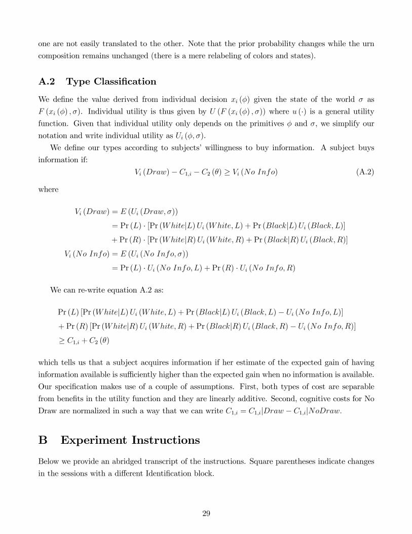
We de�ne our types according to subjects�willingness to buy information. A subject buys

information if:

Vi (Draw)� C1;i � C2 (�) � Vi (No Info) (A.2)

where

Vi (Draw) = E (Ui (Draw; �))

= Pr (L) � [Pr (WhitejL)Ui (White; L) + Pr (BlackjL)Ui (Black; L)]+ Pr (R) � [Pr (WhitejR)Ui (White; R) + Pr (BlackjR)Ui (Black;R)]

Vi (No Info) = E (Ui (No Info; �))

= Pr (L) � Ui (No Info; L) + Pr (R) � Ui (No Info;R)

We can re-write equation A.2 as:

Pr (L) [Pr (WhitejL)Ui (White; L) + Pr (BlackjL)Ui (Black; L)� Ui (No Info; L)]+ Pr (R) [Pr (WhitejR)Ui (White; R) + Pr (BlackjR)Ui (Black;R)� Ui (No Info;R)]� C1;i + C2 (�)

which tells us that a subject acquires information if her estimate of the expected gain of having

information available is su¢ ciently higher than the expected gain when no information is available.

Our speci�cation makes use of a couple of assumptions. First, both types of cost are separable

from bene�ts in the utility function and they are linearly additive. Second, cognitive costs for No

Draw are normalized in such a way that we can write C1;i = C1;ijDraw � C1;ijNoDraw:

B Experiment Instructions

Below we provide an abridged transcript of the instructions. Square parentheses indicate changes

in the sessions with a di¤erent Identi�cation block.

29

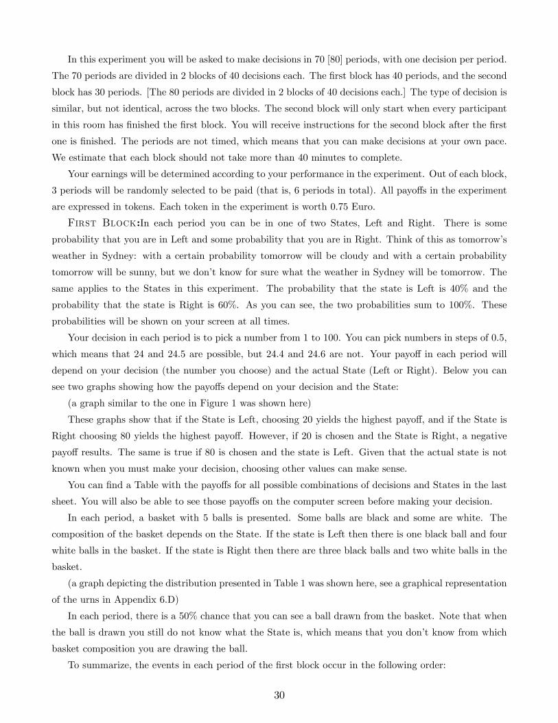
In this experiment you will be asked to make decisions in 70 [80] periods, with one decision per period.

The 70 periods are divided in 2 blocks of 40 decisions each. The �rst block has 40 periods, and the second

block has 30 periods. [The 80 periods are divided in 2 blocks of 40 decisions each.] The type of decision is

similar, but not identical, across the two blocks. The second block will only start when every participant

in this room has �nished the �rst block. You will receive instructions for the second block after the �rst

one is �nished. The periods are not timed, which means that you can make decisions at your own pace.

We estimate that each block should not take more than 40 minutes to complete.

Your earnings will be determined according to your performance in the experiment. Out of each block,

3 periods will be randomly selected to be paid (that is, 6 periods in total). All payo¤s in the experiment

are expressed in tokens. Each token in the experiment is worth 0.75 Euro.

First Block:In each period you can be in one of two States, Left and Right. There is some

probability that you are in Left and some probability that you are in Right. Think of this as tomorrow�s

weather in Sydney: with a certain probability tomorrow will be cloudy and with a certain probability

tomorrow will be sunny, but we don�t know for sure what the weather in Sydney will be tomorrow. The

same applies to the States in this experiment. The probability that the state is Left is 40% and the

probability that the state is Right is 60%. As you can see, the two probabilities sum to 100%. These

probabilities will be shown on your screen at all times.

Your decision in each period is to pick a number from 1 to 100. You can pick numbers in steps of 0.5,

which means that 24 and 24.5 are possible, but 24.4 and 24.6 are not. Your payo¤ in each period will

depend on your decision (the number you choose) and the actual State (Left or Right). Below you can

see two graphs showing how the payo¤s depend on your decision and the State:

(a graph similar to the one in Figure 1 was shown here)

These graphs show that if the State is Left, choosing 20 yields the highest payo¤, and if the State is

Right choosing 80 yields the highest payo¤. However, if 20 is chosen and the State is Right, a negative

payo¤ results. The same is true if 80 is chosen and the state is Left. Given that the actual state is not

known when you must make your decision, choosing other values can make sense.

You can �nd a Table with the payo¤s for all possible combinations of decisions and States in the last

sheet. You will also be able to see those payo¤s on the computer screen before making your decision.

In each period, a basket with 5 balls is presented. Some balls are black and some are white. The

composition of the basket depends on the State. If the state is Left then there is one black ball and four

white balls in the basket. If the state is Right then there are three black balls and two white balls in the

basket.

(a graph depicting the distribution presented in Table 1 was shown here, see a graphical representation

of the urns in Appendix 6.D)

In each period, there is a 50% chance that you can see a ball drawn from the basket. Note that when

the ball is drawn you still do not know what the State is, which means that you don�t know from which

basket composition you are drawing the ball.

To summarize, the events in each period of the �rst block occur in the following order:

30

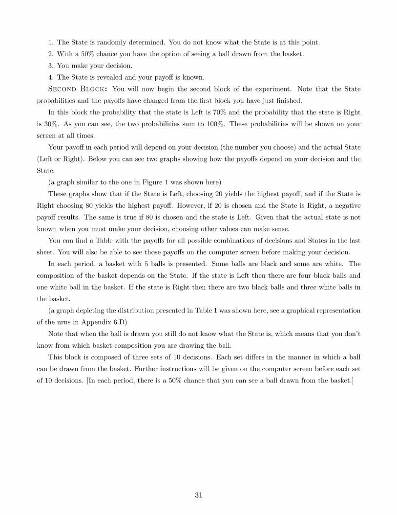
1. The State is randomly determined. You do not know what the State is at this point.

2. With a 50% chance you have the option of seeing a ball drawn from the basket.

3. You make your decision.

4. The State is revealed and your payo¤ is known.

Second Block: You will now begin the second block of the experiment. Note that the State

probabilities and the payo¤s have changed from the �rst block you have just �nished.

In this block the probability that the state is Left is 70% and the probability that the state is Right

is 30%. As you can see, the two probabilities sum to 100%. These probabilities will be shown on your

screen at all times.

Your payo¤ in each period will depend on your decision (the number you choose) and the actual State

(Left or Right). Below you can see two graphs showing how the payo¤s depend on your decision and the

State:

(a graph similar to the one in Figure 1 was shown here)

These graphs show that if the State is Left, choosing 20 yields the highest payo¤, and if the State is

Right choosing 80 yields the highest payo¤. However, if 20 is chosen and the State is Right, a negative

payo¤ results. The same is true if 80 is chosen and the state is Left. Given that the actual state is not

known when you must make your decision, choosing other values can make sense.

You can �nd a Table with the payo¤s for all possible combinations of decisions and States in the last

sheet. You will also be able to see those payo¤s on the computer screen before making your decision.

In each period, a basket with 5 balls is presented. Some balls are black and some are white. The

composition of the basket depends on the State. If the state is Left then there are four black balls and

one white ball in the basket. If the state is Right then there are two black balls and three white balls in

the basket.

(a graph depicting the distribution presented in Table 1 was shown here, see a graphical representation

of the urns in Appendix 6.D)

Note that when the ball is drawn you still do not know what the State is, which means that you don�t

know from which basket composition you are drawing the ball.

This block is composed of three sets of 10 decisions. Each set di¤ers in the manner in which a ball

can be drawn from the basket. Further instructions will be given on the computer screen before each set

of 10 decisions. [In each period, there is a 50% chance that you can see a ball drawn from the basket.]

31

C Additional results

In Table 5 there are two di¤erent models estimated. The model of column (2), an extension of the

model presented in expression 4, is:

lnr

1� r = � + � ln�Pr (Left)

Pr (Right)

�+ �1 �DCostly + �2 �DForced

+ (�1 + �2 �DCostly + �3 �DForced) � ln�Pr (DrawjL)Pr (DrawjR)

�The addition of the dummy variables in model 2 explicitly allows the possibility that the

Costly and Forced treatments have an e¤ect on individual decisions through channels other than

representativeness (i.e. through the constant � or the scope of the base rate bias ). Table 11

presents additional regressions of the estimation of model (4) presented in Section 3.2. Columns

(1) and (2) are identical to the columns presented in Table 5. Columns (3) and (4) include the

same independent variables as Columns (1) and (2), respectively, but in the number of observation

used. In these regressions observation of subjects who make decisions outside x 2 [20; 80] are

discarded.

Model(1) (2) (3) (4)

�1 (Likelihood ratio) 1:19��� 1:20��� 1:02��� 1:02���

(0:16) (0:16) (0:14) (0:13)�2 (Likelihood ratio x Costly) 0:55�� 0:53�� 0:46� 0:45��

(0:26) (0:26) (0:23) (0:22)�3 (Likelihood ratio x Forced) 0:64�� 0:64�� 0:61�� 0:63��

(0:31) (0:32) (0:29) (0:28)Costly � �0:08 � �0:03

� (0:09) � (0:09)Forced � 0:02 � 0:08

� (0:11) � (0:10)Constant �0:24 �0:21 �0:27 �0:28

N 443 443 385 385

Table 11: Representativeness bias and treatment e¤ects Note: Clustered standard errors used. ���=��=�indicates signi�cancelevel at the 1%=5%=10%.

Table 12 presents average aggregate decision by subjects types and ball draw. Table 13 is

identical to Table 8, with the control variables explicitly shown. Math has a signi�cant e¤ect after

both draws. A larger number of math courses leads to a shift towards less extreme decision making.

Gender has a signi�cant e¤ect only after a Black draw. Female subjects also tend towards less

extreme decisions. Risk does have a signi�cant e¤ect. It is worth mentioning that our measure of

risk is truncated at risk neutrality (Risk 2 [0; 3] where Risk = 3 is risk neutrality). Our measure

32

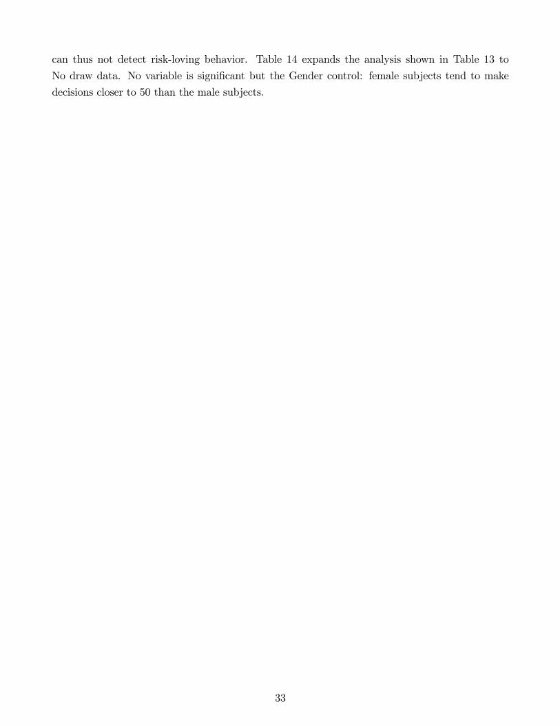
can thus not detect risk-loving behavior. Table 14 expands the analysis shown in Table 13 to

No draw data. No variable is signi�cant but the Gender control: female subjects tend to make

decisions closer to 50 than the male subjects.

33

Blackdraw

Whitedraw

Nodraw

Type1Type2Type3

Type1Type2Type3

Type1Type2Type3

Free

57:15

67:05

72:35

52:94

41:14

40:91

56:91

54:31

56:71

(5:63)

(2:17)

(2:00)

(7:88)

(2:26)

(2:83)

(3:1)

(1:13)

(1:53)

Costly

80:5

67:14

72:74

3940:55

34:56

52:31

55:38

58:06

(19:5)

(2:60)

(2:19)

(�)

(4:02)

(2:62)

(1:64)

(1:91)

(1:15)

Forced

65:5

72:01

72:14

37:67

35:30

34:28

63:33

57:13

52:07

(�)

(2:09)

(2:20)

(3:17)

(3:16)

(2:24)

(4:04)

(1:35)

(2:09)

Table12:Decisionmeansbytypes.Standarderrorsinbrackets.Emptybracketsindicateonlyoneobservation.

34

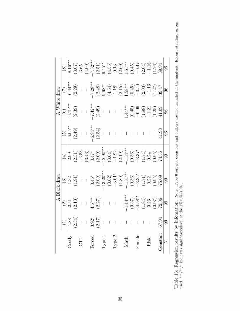
ABlackdraw

AWhitedraw

(1)

(2)

(3)

(4)

(5)

(6)

(7)

(8)

Costly

1:88

2:51

1:32

2:99

�6:05��

�6:79����6:44����8:16���

(2:34)

(2:13)

(1:91)

(2:31)

(2:49)

(2:39)

(2:29)

(3:07)

CT2

��

��3:58

��

�3:65

��

�(3:43)

��

�(4:00)

Forced

3:92�

4:67��

3:46�

3:47�

�6:94����7:42����7:28����7:32���

(2:17)

(2:27)

(2:09)

(2:09)

(2:54)

(2:49)

(2:48)

(2:51)

Type1

��

�13:20���

�12:90���

��

9:68��

9:45��

��

(3:62)

(3:64)

��

(4:54)

(4:55)

Type2

��

�3:01�

�1:92

��

1:18

0:13

��

(1:80)

(2:19)

��

(2:15)

(2:60)

Math

��1:14���

�1:31���

�1:34���

�1:44���

1:58���

1:61���

�(0:37)

(0:36)

(0:36)

�(0:45)

(0:45)

(0:45)

Female

��4:58��

�3:35�

�3:37�

��0:06

�0:50

�0:47

�(1:84)

(1:71)

(1:74)

�(1:98)

(2:03)

(2:04)

Risk

�0:23

0:22

0:24

��1:21

�1:16

�1:16

�(0:97)

(0:95)

(0:95)

�(1:25)

(1:27)

(1:26)

Constant

67:94

72:06

75:09

74:56

41:98

41:09

39:47

39:94

N99

9999

9996

9696

96

Table13:Regressionresultsbyinfomation.

Note:Type0subjectdecisionsandoutliersarenotincludedintheanalysis.Robuststandarderrors

used.��� =��=�indicatessigni�cancelevelatthe1%=5%=10%:.

35

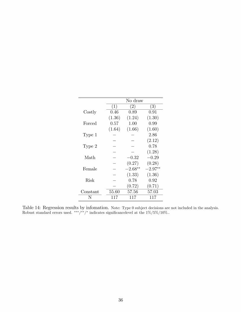
No draw(1) (2) (3)

Costly 0:46 0:89 0:91(1:36) (1:24) (1:30)

Forced 0:57 1:00 0:99(1:64) (1:66) (1:60)

Type 1 � � 2:86� � (2:12)

Type 2 � � 0:78� � (1:28)

Math � �0:32 �0:29� (0:27) (0:28)

Female � �2:68�� �2:97��� (1:33) (1:36)

Risk � 0:78 0:92� (0:72) (0:71)

Constant 55:60 57:56 57:03N 117 117 117

Table 14: Regression results by infomation. Note: Type 0 subject decisions are not included in the analysis.Robust standard errors used. ���=��=� indicates signi�cancelevel at the 1%=5%=10%:.

36

37

D Snapshot of the Experiment

Below we reproduce snapshots of the practice questions:

38

Below we reproduce a snapshot of the experiment (Free treatment):