Time-Varying E¤ects of Oil Supply Shocks on the US

Economy�

Christiane BaumeisterGhent University

christiane.baumeister@ugent.be

Gert PeersmanGhent University

gert.peersman@ugent.be

This version: September 2008

First version: November 2007

Abstract

We investigate how the dynamic e¤ects of oil supply shocks on the US economy

have changed over time. We �rst document a remarkable structural change in the oil

market itself, i.e. a considerably steeper, hence, less elastic oil demand curve since

the mid-eighties. Accordingly, a typical oil supply shock is currently characterized

by a much smaller impact on world oil production and a greater e¤ect on the real

price of crude oil, but has a similar impact on US output and in�ation as in the

1970s. Second, we �nd a smaller role for oil supply shocks in accounting for real

oil price variability over time, implying that current oil price �uctuations are more

demand driven. Finally, while unfavorable oil supply disturbances explain little of

the "Great In�ation", they seem to have contributed to the 1974/75, early 1980s and

1990s recessions but also dampened the economic boom at the end of the millennium.

JEL classi�cation: E31, E32, Q43

Keywords: Oil prices, vector autoregressions, time-varying coe¢ cients

�We thank Luca Benati, Jean Boivin, Luca Gambetti, Domenico Giannone, James Hamilton, Morten

Ravn, Frank Smets, Herman van Dijk and Timo Wollmershäuser as well as conference participants at

the CESifo Munich, IWH Halle, EEA-ESEM Milan and seminar participants at the Erasmus University

Rotterdam and the University of Kent for their useful comments and suggestions. Special thanks to Lutz

Kilian for many insightful discussions and feedback on an earlier version of the paper. We acknowledge

�nancial support from the Interuniversity Attraction Poles Programme - Belgian Science Policy [Contract

No. P6/07] and the Belgian National Science Foundation. All remaining errors are ours.

1

1 Introduction

The belief that physical disruptions in the supply of crude oil in the world oil market are at

the origin of stag�ationary episodes has gained ground in the wake of the two big oil shocks

of the 1970s.1 Since that time oil price increases are associated in many people�s minds

with severe macroeconomic consequences in terms of higher in�ation and lower economic

growth. A remarkable feature of the recent, prolonged surge in oil prices however, is

the relatively mild impact this seems to exert on real economic activity and the price

level. This observation casts doubt on the relevance of oil shocks for the macroeconomic

performance of the US economy in more recent times. In other words, the way the economy

experiences oil shocks appears to have changed fundamentally. This conjecture has recently

been con�rmed in the empirical literature by Edelstein and Kilian (2007a), Herrera and

Pesavento (2007) and Blanchard and Galí (henceforth, BG 2007). In particular, these

studies �nd a reduced impact of oil price shocks on US macroeconomic aggregates over

time. The objective of this paper is to further investigate how the dynamic e¤ects of oil

supply disturbances have changed and whether global oil supply shocks can be considered

as an important source of economic �uctuations. We evaluate the importance of physical

production shortfalls in explaining �uctuations in the real price of oil as well as their

contribution to the observed movements in US real GDP growth and consumer price

in�ation when time variation is accounted for.

The main results that emerge from our analysis are the following. We foremost doc-

ument a remarkable structural change in the global oil market. Speci�cally, a "typical"

oil supply shock is characterized by a much smaller impact on world oil production and

a greater e¤ect on the real price of crude oil since the second half of the 1980s. Only

a steeper, hence, less elastic oil demand curve can explain this stylized fact. This �nd-

ing has important consequences when the macroeconomic e¤ects of oil supply shocks are

compared over time. If a comparison is based on a similar change of crude oil prices (e.g.

a 10 percent rise), we currently �nd a more muted impact on the US economy which

is consistent with the existing evidence for oil price shocks. This comparison, however,

cannot really be made because a di¤erent underlying oil supply shock is considered. In

particular, a constant slope of the oil demand curve is implicitly assumed which is at odds

with our evidence. On the other hand, if an exogenous oil supply shock is measured as

a similar shift in world oil production (e.g. a production shortfall of 1 percent), such a

disturbance has a much greater impact on oil prices now, resulting also in stronger e¤ects

1Hamilton (1983) was the �rst to notice that all but one of the US postwar recessions have followed

sharp increases in the price of crude oil.

2

on real GDP and consumer prices compared to the 1970s and early 1980s. However, also

this comparison is biased since an average oil supply shock is characterized by a distur-

bance in oil production of more than 2 percent in the 1970s and hardly 0.5 percent since

the 1990s. When we consider a typical one standard deviation oil supply shock instead,

we �nd a rather similar impact on US macroeconomic aggregates over time. In addition,

oil supply disturbances consistently account for 15 to 20 percent of output and in�ation

variability.

If the e¤ects of average oil supply shocks have not dramatically changed since the

1970s, it is surprising that we are currently not confronted with similar macroeconomic

conditions. To explain this, we demonstrate that oil supply shocks explain little of the

Great In�ation, which is consistent with the propositions of Barsky and Kilian (henceforth,

BK 2002, 2004). In addition, oil supply disturbances seem to have played a signi�cant but

certainly non-exclusive role in the 1974/75, early 1980s and 1990s recessions; by the same

token, unfavorable oil supply shocks in 1999 made a signi�cant negative contribution to

the ongoing boom at the end of the millennium. Moreover, we show that the contribution

of oil supply shocks to �uctuations in the real price of oil has decreased over time which

means that current oil price movements are more demand driven. Despite a relatively

constant share of oil supply shocks in explaining the variance of oil production growth

(being constantly around 30 percent) and the aforementioned higher leverage e¤ect on oil

prices, the latter �nding implies that also the oil supply curve is currently more inelastic.

A steepening of both the oil demand and oil supply curves can be considered as a source

of increased oil price volatility in more recent times.

The analysis in this paper departs from the existing literature along two dimensions.

First, the paper makes use of recent methodological contributions in explicitly modeling

time variation. Instabilities over time in the crude oil market and the oil-macro relation-

ship have been widely documented in the literature.2 On the one hand, the oil market

itself has undergone substantial changes. Global capacity utilization rates in crude oil pro-

duction have not been constant over time, with production levels being above sustainable

capacity since the late 1980s, as well as in 1973/74 and 1979/80 (Kilian 2008c). In addi-

tion, the transition from a regime of administered oil prices to a market-based system of

direct trading in the spot market and the collapse of the OPEC cartel in late 1985 were ac-

companied by a dramatic rise in oil price volatility (e.g. Hubbard 1986). Furthermore, the

relative importance of the driving forces behind oil price movements has changed (e.g. BK

2Structural breaks in the relationship between oil prices and the macroeconomy were initially docu-

mented by Mork (1989) and Hooker (1996, 2002), when sample periods were extended to include data

from the mid-1980s onwards.

3

2002, 2004; Hamilton 2003, 2008a; Rotemberg 2007).3 On the other hand, also the macro-

economic structure has changed over time which can bring about time-varying e¤ects of oil

shocks.4 Prominent explanations for di¤erent macroeconomic consequences of oil shocks

over time discussed in the literature are improved monetary policy (e.g. Bernanke et al.

1997; BG 2007),5 more �exible labor markets (BG 2007), changes in the composition of

automobile production and the overall importance of the US automobile sector (Edelstein

and Kilian 2007b), and variations in the role and share of oil in the economy over time

(e.g. Bernanke 2006; BG 2007). Other arguments for changing macroeconomic e¤ects of

oil shocks that have been put forward are time-varying mark-ups of �rms (Rotemberg and

Woodford 1996) and changes in �rms�capacity utilization (Finn 2000).

All these changes suggest that a linear, constant-coe¢ cient speci�cation may not ac-

curately capture the e¤ects of oil supply shocks on the US economy. Consequently, time

variation has to be allowed for in order to adequately model the interaction between oil

shocks and aggregate economic activity and to explore how this relationship has evolved

over time. Several studies, using a vector autoregression approach (e.g. Edelstein and

Kilian 2007a; Herrera and Pesavento 2007), take time variation into account by splitting

the sample into two subperiods assuming a structural break sometime in the 1980s.6 Al-

ternatively, BG (2007) allow for a more gradual variation over time by estimating bivariate

vector autoregressions over rolling time windows.7 To model time variation, we estimate a

multivariate time-varying parameters Bayesian vector autoregression (TVP-BVAR) with

stochastic volatility for the period 1970Q1-2006Q2 in the spirit of Cogley and Sargent

(2002, 2005), Canova and Gambetti (2004) and Benati and Mumtaz (2007). The varying

coe¢ cients are meant to capture smooth transitions in the propagation mechanism of oil

shocks without imposing a speci�c breakpoint, while the stochastic volatility component

models changes in the magnitude of structural shocks and their immediate impact. The

latter feature is particularly important in the present setting given the documented in-

creased volatility in the oil market and the reduced macroeconomic volatility. By using

3Lee, Ni and Ratti (1995) and Ferderer (1996) argue that the increased volatility has led to a breakdown

of the empirical relationship between oil prices and economic activity in the US since the mid-eighties.

Kilian (2008a,b) stresses that shifts in the composition of oil supply and oil demand shocks driving the

price of oil help explain why regressions of macroeconomic aggregates on oil prices tend to be unstable

over time and lead to the changing e¤ects of oil price shocks.4These structural changes are very much related to the literature on the "Great Moderation". See, for

instance, McConnell and Pérez-Quirós (2000), Blanchard and Simon (2001) and Stock and Watson (2003).5This argument has been de�ed by Hamilton and Herrera (2004) and Herrera and Pesavento (2007).6The break date is mostly chosen in relation to the start of the Great Moderation in 1984 or the oil

price plunge in early 1986.7De Gregorio et al. (2007) use a similar approach for the pass-through of oil price shocks to in�ation.

4

a multivariate approach, it is also possible to learn more about potential sources of time

variation.

Second, we propose a new identi�cation strategy to isolate the unanticipated move-

ments in the price of crude oil due to exogenous supply shocks. Most studies, including

BG (2007), rely on a recursive identi�cation scheme where all variations in oil prices are

assumed to be oil supply shocks. This view, however, has been challenged in the recent

literature. BK (2002), for instance, argue that the oil price rises of the seventies might

be the result of expansionary monetary policy and Kilian (2008c) shows that only a small

fraction of observed oil price �uctuations can be attributed to exogenous oil production

disruptions. Therefore Kilian (2008a), based on the assumption of a vertical short-run

supply curve, identi�es oil supply shocks as the only source of innovations in global oil

production, whereas shocks to the demand for crude oil have an immediate e¤ect only on

oil prices in a monthly VAR. His identifying assumptions are, however, less appropriate

for estimations with quarterly data such as real GDP. For that reason he uses a single-

equation approach to estimate, in a second step, the impact of quarterly shocks on US

real GDP and CPI in�ation by averaging the monthly structural innovations over each

quarter.8

To allow for an immediate e¤ect of both oil supply and oil demand shocks on oil

production and the real price of crude oil, we propose to use sign restrictions instead, to

identify oil supply shocks in a quarterly VAR.9 Speci�cally, the sign restrictions are derived

from a simple supply and demand model of the world oil market. Using both world oil

production and oil price data, oil supply shocks are identi�ed as the only disturbances that

displace the oil supply curve in this market. As a consequence, our method recognizes the

fact that contemporaneous movements in oil prices and oil production could also be driven

by disturbances relating to the demand for crude oil. Moreover, given our time-varying

framework, the magnitude of the contemporaneous impact of structural shocks on oil

production and prices can vary over time and hence, changes in the relative importance of

oil supply and demand shocks and the slope of both curves are captured. We also show that

our conclusions do not depend on the selected methodology and underlying assumptions.

In particular, robust results are found for alternative speci�cations, the modeling of time

variation and the identi�cation strategy.

8 In this way, Kilian (2008a) also demonstrates that the exact underlying source of oil price movements

is crucial for the subsequent economic consequences.9See Faust (1998), Canova and De Nicoló (2002), Uhlig (2005) and Peersman and Straub (2005) for

alternative applications of this identi�cation strategy. In particular, Peersman (2005) uses sign restrictions

to identify oil shocks but without including world oil production.

5

The remainder of the paper is structured as follows. Section 2 presents the methodology

and describes the identi�cation strategy in more detail. Section 3 discusses the main

empirical results and evaluates the robustness of our �ndings. In section 4, we discuss

some potential explanations for a less elastic oil demand curve in more recent periods, and

section 5 o¤ers some concluding remarks.

2 Methodology

2.1 A VAR with time-varying parameters and stochastic volatility

We model the joint behavior of global oil production, the real re�ner acquisition cost of

imported crude oil,10 US real GDP and US CPI as a VAR with time-varying parameters:11

yt = ct +B1;tyt�1 + :::+Bp;tyt�p + ut � X 0t�t + ut (1)

The frequency of our data is quarterly and the overall sample covers the period 1947Q1-

2006Q2. The �rst twenty years of data are, however, used as a training sample to generate

the priors for the actual sample period.12 The lag length is set to p = 4 to allow for suf-

�cient dynamics in the system.13 The time-varying intercepts and lagged coe¢ cients are

stacked in �t to obtain the state-space representation of the model. The ut of the obser-

vation equation are heteroskedastic disturbance terms with zero mean and a time-varying

covariance matrix t which can be decomposed in the following way: t = A�1t Ht�A�1t

�0.

At is a lower triangular matrix that models the contemporaneous interactions among the

10This oil price variable measures most accurately the marginal cost of crude oil to US re�ners. It is

therefore the best proxy for the free market global price of imported crude oil. For di¤erent concepts of

world oil prices, see Mabro (2005). We have checked the sensitivity of our results to alternative oil price

measures such as the WTI spot oil price and the composite re�ner acquisition cost; our conclusions are not

altered by the choice of this variable. Results are available upon request.11All variables are transformed to non-annualised quarter-on-quarter rates of growth by taking the �rst

di¤erence of the natural logarithm. The nominal re�ner acquisition cost has been de�ated using the US

CPI. A detailed description of all the data used in this paper can be found in Appendix A.12We have also experimented with shorter sample periods to calibrate our priors. Given su¢ ciently

di¤use priors, our results were not altered by the choice of the training sample.13An appropriate lag structure is necessary to adequately capture the dynamics contained in the data.

Since most studies in this literature opt for a lag order of four quarters, we also choose this for reasons

of comparability. Moreover, Hamilton and Herrera (2004) also argue that too short a lag length might

omit the primary e¤ects of oil shocks. However, our �ndings are qualitatively similar when less lags are

included.

6

endogenous variables and Ht is a diagonal matrix which contains the stochastic volatilities:

At =

2666641 0 0 0

�21;t 1 0 0

�31;t �32;t 1 0

�41;t �42;t �43;t 1

377775 Ht =

266664h1;t 0 0 0

0 h2;t 0 0

0 0 h3;t 0

0 0 0 h4;t

377775 (2)

The drifting coe¢ cients are meant to capture possible nonlinearities or time variation

in the lag structure of the model. The multivariate time-varying variance covariance

matrix allows for heteroskedasticity of the shocks and time variation in the simultaneous

relationships between the variables in the system. Allowing for time variation in both

the coe¢ cients and the variance covariance matrix, leaves it up to the data to determine

whether the time variation of the linear structure comes from changes in the size of the

shock and its contemporaneous impact (impulse) or from changes in the propagation

mechanism (response). Given the observed instabilities in the oil-macro relationship, this

approach is particularly expedient. Let �t be the vector of non-zero and non-one elements

of the matrix At (stacked by rows) and ht be the vector containing the diagonal elements

of Ht. Following Primiceri (2005), the three driving processes of the system are postulated

to evolve as follows:

�t = �t�1 + �t �t � N (0; Q) (3)

�t = �t�1 + �t �t � N(0; S) (4)

lnhi;t = lnhi;t�1 + �i�i;t �i;t � N(0; 1) (5)

The time-varying parameters �t and �t are modeled as driftless random walks.14 In

line with Primiceri (2005) we do not impose a stability constraint on the evolution of the

time-varying parameters to enforce stationarity of the VAR system.15 The elements of the

vector of volatilities ht = [h1;t; h2;t; h3;t; h4;t]0 are assumed to evolve as geometric random

walks independent of each other.16 The error terms of the three transition equations are

14Canova and Gambetti (2004) have also experimented with more general autoregressive processes for

the law of motion of the coe¢ cients but report that the random walk speci�cation was always preferred.

Moreover, as has been pointed out by Primiceri (2005), the random walk assumption has the desirable

property of focusing on permanent parameter shifts and reducing the number of parameters to be estimated.15 Initially, we have included an indicator function which selected only stable draws i.e. the indicator

function I (�t) = 0 if the roots of the associated VAR polynomial are inside the unit circle as e.g. in Cogley

and Sargent (2005). However, our acceptance ratio was so high as to make this constraint obsolete.16Stochastic volatility models are typically used to infer values for unobservable conditional volatilities.

The main advantage of modelling the heteroskedastic structure of the innovation variances by a stochastic

volatility model as opposed to the more common GARCH speci�cation lies in its parsimony and the

7

independent of each other and of the innovations of the observation equation. In addition,

we impose a block-diagonal structure for S of the following form:

S � V ar (�t) =

264 S1 01x2 01x3

02x1 S2 02x3

03x1 03x2 S3

375 (6)

which implies independence also across the blocks of S with S1 � V ar��21;t

�, S2 �

V ar���31;t; �32;t

�0�, and S3 � V ar ���41;t; �42;t; �43;t�0� so that the covariance states canbe estimated equation by equation.17

We estimate the above model using Bayesian methods. An overview of the prior spec-

i�cations and the estimation strategy (Markov Chain Monte Carlo algorithm) is provided

in Appendix B.

2.2 Identi�cation of oil supply shocks

Separating the endogenous and exogenous sources of movements in the price of crude oil

has proven to be a di¢ cult task. In most VAR-based studies (e.g. Burbidge and Harrison

1984; Jiménez-Rodríguez and Sánchez 2005; BG 2007) oil supply shocks are identi�ed

as innovations in the oil price variable.18 Treating the unpredictable variations in the

price of oil as exogenous with respect to the developments in the US economy (and more

generally, global macroeconomic forces) �nds its origin in the belief that at least the major

oil price shocks were due to production shortfalls caused by political events in the Middle

East. Implicit in this view is the assumption that oil price changes derive exclusively from

the supply side of the oil market. However, it is now commonly accepted that oil prices,

especially in more recent decades, are also driven by demand conditions (see BK 2002,

2004; Hamilton 2003, 2008a; Kilian 2008a; Rotemberg 2007). Consequently, innovations

in the oil price equation of a VAR are not necessarily an adequate measure of exogenous

variations in oil supply since they may also capture shifts in the demand for crude oil.

In that sense, the resulting estimates only represent the economic e¤ects of an average

oil price shock determined by a combination of supply as well as demand factors which

independence of conditional variance and conditional mean. Put di¤erently, changes in the dependent

variable are driven by two di¤erent random variables since the conditional mean and the conditional

variance evolve separately. Implicit in the random walk assumption is the view that the volatilities evolve

smoothly.17As has been shown by Primiceri (2005, Appendix D), this assumption can be easily relaxed.18A lot of studies employ nonlinear transformations of the oil price, such as the net oil price index

(Hamilton 1996, 2003), as a measure of exogenous supply shocks which already takes asymmetries into

account. However, it is even less clear how to interpret a (negative) innovation to such a �ltered variable.

8

can bias the estimates.19 This concern is even more relevant in a time-varying context,

in particular when the relative importance of oil supply versus oil demand shocks has

changed over time. Others (e.g. BG 2007) have made the case that this distinction does

not matter since an oil price shock triggered by increased demand for oil in one country

can still be experienced as a supply shock by the remaining countries. This presumption

is, however, very stringent in the light of the results of Kilian (2008a) and Peersman and

Van Robays (2008) who show that there exist important di¤erences in the responses of

macroeconomic aggregates depending on the underlying source of the oil shock. Intuitively

it is clear that an increase in the price of oil induced by favorable global economic conditions

exerts a di¤erent in�uence on the macroeconomic performance than one due to oil supply

interruptions resulting from a war (see Rotemberg 2007).20 Moreover, considering only

oil prices also implicitly assumes that the slope of the oil demand curve remains constant

over time. However, if the elasticity of the demand curve is not invariant over the sample

period, a similar physical disruption in the supply of crude oil due to e.g. a military con�ict,

will have a very di¤erent impact on the oil price itself which complicates intertemporal

comparisons. In section 3, we will show that the slope of the demand curve has indeed

changed over time.

A di¤erent strand of the literature has developed measures based on physical oil supply

disruptions associated with major political crises in oil-producing countries in order to ex-

tract the magnitude of exogenous oil supply shocks. Hamilton (2003) uses a quantitative

version of the dummy-variable approach (Dotsey and Reid 1992) to isolate the exogenous

component of oil price movements by measuring the oil supply curtailed by exogenous

events which are largely political in origin.21 He compares the observed production level

before a military con�ict started with the largest drop of oil supply in the a¤ected coun-

tries in subsequent periods. The magnitude of the production shortfall is then de�ned as

the exogenous oil supply shock expressed as a percentage of world oil production. Kilian

(2008c) constructs an alternative measure of exogenous oil supply shocks by comparing the

actual production shortfalls in the wake of a political crisis to an explicit counterfactual

path of how production would have evolved in the absence of the crisis. The counterfac-

tual production level is derived from countries which are subject to the same economic

incentives but not involved in the con�ict. While these methods avoid potential problems

19Despite its innovative oil futures-based identi�cation approach, the study by Anzuini et al. (2007) is

also prone to fall prey to this criticism because they also mix supply and precautionary demand shocks.20See also De Gregorio et al. (2007) who point to the link between the nature of the oil shock and the

compensatory movements that the driving force behind the oil price increase exerts on the exchange rate.21The events Hamilton (2003) considers are the Suez crisis (1956), the Arab-Israel war (1973), the Iranian

revolution (1978), the Iran-Iraq war (1980-1988) and the Persian Gulf war (1990/91).

9

regarding the endogeneity of the oil price series, a shortcoming is that they are closely tied

to a selection of relevant historical episodes and no generic supply shocks are identi�ed.22

Kilian (2008a) allows shocks to the demand for crude oil to have a contemporaneous im-

pact on oil prices in a monthly vector autoregression. To identify an oil supply shock, he

assumes that the latter is the only disturbance which has an immediate in�uence on the

level of oil production. Accordingly, shifts in the demand for oil only have a delayed e¤ect

on crude oil production, i.e. a vertical short-run supply curve is assumed. This assumption

is, however, less appropriate when quarterly data are used like in our study. In addition,

oil production could already react to expected shifts in economic activity which are not

fully captured in such a setting.

Elaborating on work by Faust (1998), Canova and De Nicoló (2002), Uhlig (2005),

Peersman (2005), Peersman and Straub (2005) and Benati and Mumtaz (2007), we pro-

pose to use sign restrictions on the estimated time-varying impulse responses to identify

structural oil supply shocks. More speci�cally, the restrictions are derived from a sim-

ple textbook supply and demand model for the global oil market. In the spirit of Kilian

(2008a), we present the global oil market by world oil production and the world crude

oil price. An oil supply shock is identi�ed as any shift in the oil supply curve and hence,

results in an opposite movement of oil production and the real price of crude oil.23 In

particular, the identifying assumptions are that after an unfavorable oil supply shock

world oil production does not increase and the real price of crude oil does not decrease.24

These restrictions are su¢ cient to uniquely identify global oil supply disturbances without

having to impose zero restrictions on oil prices or production to distinguish them from

other shocks. Furthermore, no condition at all constrains the responses of real output and

consumer price in�ation. The reactions of these variables will eventually be determined

by the data. Since our focus is on the time-varying e¤ects of oil supply shocks, we only

partially identify the model. All other shocks, i.e. shocks with an impact on oil prices

and production of the same sign, are considered as oil demand shocks. These could be

oil-speci�c demand shocks or shifts in the oil demand curve resulting from changes in

economic activity.25 We impose the sign conditions to be binding for four quarters fol-

lowing the shock. Consequently, our restrictions accommodate a potential sluggishness

22Also Anzuini et al. (2007) heavily rely upon the use of previously selected exogenous events.23For illustrative purposes of our identi�cation assumptions, we refer the reader to Figure 3, panel A.24These restrictions are imposed as weak inequality constraints � and �, thus including also the possi-

bility of no change, i.e. a zero response. As a consequence of these inequality contraints, our identi�cation

scheme does not deliver exact identi�cation. See Fry and Pagan (2007) for a discussion of this type of

restrictions and potential problems.25 In Baumeister and Peersman (2008), we also estimate the impact of di¤erent oil demand shocks, in

particular oil-market speci�c demand shocks and global shocks in economic activity.

10

in the adjustment of the oil market. Some robustness checks with regard to alternative

restrictions and the horizon over which the sign constraints are imposed are conducted in

section 3.3. The details for the computation of the time-varying impulse responses and

the implementation of the sign restrictions are described in Appendix C.

3 Results

3.1 Impulse responses

Figure 1 displays the median impulse responses of world oil production, the real price of oil,

US real GDP and US CPI to a one standard deviation oil supply shock for horizons up to

20 quarters at each point in time spanning the period 1970Q1 to 2006Q2.26 The estimated

responses have been accumulated and are shown in levels. In general, an unfavorable oil

supply shock results in a permanent fall of oil production and a permanent rise of the real

re�ner acquisition cost of imported crude oil. Consistent with expectations, the shock is

followed by a signi�cant slowdown in real economic activity and increases in consumer

prices, variables which were not constrained. This evidence emerges even more clearly

in Figure 2, panel A, where the time-varying median responses of the four variables are

plotted four quarters after the shock,27 together with the 16th and 84th percentiles of the

posterior distribution. Speci�cally, after a representative oil supply shock, we observe a

relatively similar impact on output over time, which is statistically more signi�cant in

the second half of the sample, as well as slightly stronger in�ationary e¤ects.28 We also

performed some bilateral tests for time variation to measure the statistical signi�cance

of di¤erences over time. For this purpose, we sample 10,000 impulse responses from

the posterior distribution of each quarter and calculate the di¤erence with draws from

the posterior of some benchmark periods.29 For several benchmark quarters, we �nd a

26The 3D-graphs of the time-varying impulse responses are to be read in the following way: along the

x-axis the starting quarters are aligned from 1970Q1 to 2006Q2, on the y-axis the quarters after the shock

are displayed, and on the z-axis the value of the response is shown in percent. All responses have been

normalized in such a way that the structural innovations raise the price of oil.27This choice can be rationalized by the fact that the greatest e¤ect on real GDP is expected to occur

with a delay of 3 to 4 quarters after the shock (Hamilton 2008a). However, given the persistency of the

responses, the message is not altered if di¤erent horizons are selected.28For real GDP, we also �nd somewhat stronger e¤ects over time for longer horizons after the shock, as

can be seen in Figure 1.29See also Gambetti (2006) for similar tests. Since this exercise generates a separate distribution for

each horizon of each quarter in the sample for all benchmark periods, we do not show the results, but they

are available upon request.

11

statistically signi�cant, stronger e¤ect of a one standard deviation oil supply shock on

consumer prices in more recent periods and for some quarters even a larger long-run

impact on output. This evidence is striking, given the results presented in Edelstein and

Kilian (2007a), Herrera and Pesavento (2007) and BG (2007), who �nd a reduced impact

on real output and consumer prices over time.

We do �nd, however, considerable time variation in the dynamics of the oil market itself

which is symptomatic of the fact that the global oil market has undergone fundamental

structural changes. By all appearances the interaction between oil production and oil

prices varies remarkably across time periods with an obvious declining trend in the response

of oil quantity and a stronger impact on the oil price level since the mid-eighties. Also for

the episodes 1973/74 and 1979/80, we observe an increased reaction of crude oil prices.

Not surprisingly, a statistically signi�cant, smaller impact on oil production and greater

e¤ect on real oil prices over time is strongly con�rmed by the bilateral tests.

A natural question which emerges is why we �nd such a change in the oil market

over time. We observe that the responses in the oil market set in immediately. Since the

magnitude of the shocks are inextricably intertwined with the contemporaneous response

of the variable in question, this feature makes it di¢ cult to distinguish between dynamics

and volatility.30 However, a change in the underlying oil supply volatility alone cannot

explain this stylized fact because the impact on oil prices and production does not change

in the same direction over time (as illustrated in panel A of Figure 3). The only possible

explanation for observing a smaller reaction of oil production in combination with a greater

reaction of oil prices is a steepening of the oil demand curve, i.e. oil demand became less

elastic over time (as shown in panel B).31 Speci�cally, in order to push up oil prices, a huge

reduction in world oil production was necessary before the mid-eighties because oil prices

were much less sensitive to changes in oil supply then as they appear to be nowadays, with

the exception of two episodes, namely 1973/74 and 1979/80.

The fact that the impact of a typical oil supply shock on oil quantity and prices changes

dramatically every period complicates, however, the analysis of the time-varying dynamic

e¤ects of an exogenous event in the oil market on the macroeconomy. The way the nor-

malization is done for the experiment becomes very important. Since the focus of previous

research has centred on an unanticipated increase in the price of oil, consider for instance,30This is a standard problem when VAR results are compared across di¤erent samples or estimated with

time-varying parameters. Only the contemporaneous impact of a shock on a number of variables can be

measured. Consequently, it is not possible to know exactly whether the shock itself (volatility) has changed

or the immediate reaction (economic structure) to this shock.31This observation does not exclude the possibility that the variability of oil supply shocks has also

changed over time, but this alone could never explain our �ndings.

12

the e¤ect of an oil supply shock which raises the real price of oil by 10 percent on impact.

The latter is used by BG (2007) as a benchmark for an intertemporal comparison. The

impact of the normalized time-varying impulse responses after four quarters are shown

in panel B of Figure 2. We �nd a more muted reaction of macroeconomic variables in

the latter part of the sample, a �nding which complies very well with existing empirical

evidence on the time-varying e¤ects of oil price shocks (e.g. BG 2007; De Gregorio et al.

2007). This experiment, however, implicitly assumes a constant slope of the oil demand

curve over time which is clearly not the case. As a consequence, the results of such a

normalization cannot be compared because a di¤erent underlying supply shock is consid-

ered. Speci�cally, a 10 percent rise in oil prices is currently generated by an oil production

shortfall of 1 to 2 percent. To elicit the same oil price move in the 1970s, a decline in the

physical supply of crude oil of up to 15 percent is required, which actually never happened

within the sample period. Despite the assertion by BG (2007) that "what matters [...] to

any given country is not the level of global oil production, but the price at which �rms and

households can purchase oil" (p.17), it appears that the volume of oil can be considered

as an important input factor in the production process.32

Alternatively, an oil supply shock can also be normalized on the quantity variable rather

than on the price variable. Oil supply shocks have frequently been viewed as physical

interruptions in the production of crude oil due to deliberate decisions by OPEC aimed at

achieving a certain price level or destruction of oil facilities in the wake of war activities.33

The dynamic macroeconomic e¤ects of exogenous oil supply shocks measured as a 1 percent

decrease in global oil production on impact are shown in panel C of Figure 2. The implied

elasticity of the real price of crude oil with respect to a 1 percent shortfall in world oil

production increases substantially over time, from an average value of 5 percent in the

1970s and 1980s to 10 percent in the 1990s up to 15 percent in the 2000s. These dramatic

oil price increases triggered by a similar reduction in oil production in the second part of

the sample are in turn more disruptive to the economy and emphasize the importance of

the proper de�nition of the oil shock concept. The accumulated loss in real GDP growth

is about twice as big in the 1990s and almost three times as big in the 2000s as in the

1970s. The response of consumer prices gets more pronounced from the 1990s onwards

and continues to increase considerably in the 2000s.34 However, also this intertemporal

32Considering only the oil price might be realistic for a small country but is more problematic for the

United States.33Since OPEC only controls the quantity supplied, the world oil price is only indirectly in�uenced. Even

if at times OPEC announced a price target or e¤ectively "set" the reference price, it still had to regulate

its production volume in order to obtain and maintain a certain price level.34This should not be too surprising since oil prices are part of the consumer price index and hence, larger

13

comparison cannot really be made since a typical (one standard deviation) shift of the

crude oil supply curve is characterized by a change in world oil production of around 2

percent in the seventies, whereas this change amounts to only 0.5 percent from the mid-

nineties onwards. Given the indistinguishability of volatility and immediate impact, our

analysis cannot determine whether these smaller average changes in oil production are

the result of a steeper oil demand curve or also the consequence of smaller shifts in the

underlying oil supply curve over time.35 ;36

3.2 Relevance of oil supply shocks

It is still a widely held belief that the oil price hikes of the 1970s and early 1980s were

the underlying source of macroeconomic stag�ation during that period (e.g. Hamilton

1983). Since the average e¤ects of oil supply shocks on US output and in�ation have not

dramatically changed compared to the 1970s, it is surprising that the current macroeco-

nomic conditions are so di¤erent. To shed some light on this issue, we now have a closer

look at the variance and historical decompositions. Figure 4 displays the median time-

varying contribution of oil supply shocks to the forecast error variance after 20 quarters

of respectively world oil production growth, changes in the real price of crude oil, US real

GDP growth and CPI in�ation together with the 16th and 84th percentiles of the posterior

distribution. The contribution of oil supply shocks to the variance of CPI in�ation and

real GDP growth in the US consistently ranges between 15 and 20 percent. The share of

output volatility attributable to oil supply shocks oscillates moderately over time, whereas

the fraction of movements in consumer price in�ation induced by unexpected oil supply

disturbances exhibits a slight increase in more recent periods. The latter is not surprising

given that the general volatility of CPI in�ation decreased over time, while the impact of

oil supply shocks on in�ation did not decline. We can thus conclude that exogenous oil

supply shocks are economically still relevant.

The decomposition also indicates that oil supply shocks account for approximately

30 percent of the forecast error variance in world oil production which only experiences

moderate variations over time. However, the �gure reveals that the contribution of oil

oil price increases automatically lead to a higher CPI even if second-round e¤ects are absent. However,

this is probably not the main reason for our �ndings since, when we employ the implicit GDP de�ator as

the measure of in�ation, we still �nd a substantial increase in the response of the price level over time.

This result is also reported in section 3.3.35 In subsequent work (Baumeister and Peersman 2008), we show that the underlying shifts of the oil

supply curve have indeed declined over time.36Note that, in case of a vertical oil supply curve, the observed decrease in oil production changes would

be fully driven by decreased oil supply volatility.

14

supply shocks to the variability in the real price of crude oil declines over time from around

30 percent in the �rst part of the sample to around 20 percent in later periods suggesting

that they are currently a less important source of oil price movements. This evidence is

consistent with Kilian (2008a,c) and the widely held belief that "demand increases rather

than supply reductions have been the primary factor driving oil prices over the last several

years" (Hamilton 2008a, p.175). Moreover, given the almost constant proportion of non-

supply shocks in world oil production and the increased contribution of these shocks to

oil price variability, our results indicate that also the oil supply curve must have become

more inelastic over time. A steeper oil supply curve is thus also a source of increased oil

price volatility.

To evaluate whether exogenous shifts of the oil supply curve are responsible for speci�c

episodes, the historical contribution of oil supply disturbances to the four endogenous

variables are presented in Figure 5. Speci�cally, these �gures show the baseline forecast

of the variables augmented by the cumulative contribution of oil supply shocks (red line)

as well as the actual time series in growth rates (blue line). The di¤erence between both

is driven by other shocks. For real GDP growth, grey bars are added to indicate periods

of recessions as dated by the NBER. With regard to in�ation, the graphs reveal that

unfavorable oil supply shocks explain little of the Great In�ation. Despite the fact that

there is a positive contribution, the bulk of excessive in�ation in the 1970s is explained

by other shocks. While this insight is apparently in contrast with popular perception,

it can still be reconciled with several recent �ndings in the literature. In particular, BK

(2002) suggest that other adverse shocks must have been at the origin of the stag�ationary

experience of the 1970s and Clarida et al. (2000) argue that bad monetary policy was the

source of the Great In�ation.

The supply-shock driven contribution to the historical evolution of the real price of

crude oil itself and economic activity changes from episode to episode. During the 1973/74

oil embargo a major part of the oil price increase is attributable to oil supply shocks but

they cannot account completely for the price spike. The contribution of oil supply shocks

to the development of the price of oil during the events of 1978-80 is more limited and

clearly indicates that this was more a demand-driven price shock mainly determined by

rising oil demand at a time of low spare capacity.37 The latter �nding con�rms BK (2002)

and Kilian (2008a) who argue that pure oil supply shocks were never the sole driving force

behind observed �uctuations in the real price of crude oil. On the other hand, a substantial

37Skeet (1980, p.164) reports that "only Saudi Arabia exhibited any strong wish to restrain the take-o¤

of price, but it no longer had the production �exibility to manage this on its own" during the events of

1979.

15

share of the oil price hike after Iraq�s invasion of Kuwait in August 1990 can be ascribed

to unfavorable oil supply shocks. As a consequence, interruptions in the supply of crude

oil did play a signi�cant role in the 1974/75, early 1980s and 1990s recessions. However,

the contribution of oil supply disturbances to the poor macroeconomic performance was

certainly not exclusive since a major part of the slowdowns is still explained by other

shocks.

But also in more recent times unfavorable oil supply shocks had signi�cant e¤ects

on real economic activity. Consider the 1999 oil supply disturbance, engineered by the

joint decision of OPEC and non-OPEC countries to cut oil production, which made an

important contribution to the oil price rise. This unfavorable shock had a negative impact

on real GDP growth and made the ongoing strong economic boom before the millennium

turnover more subdued whereas its role in the economic downturn of 2001 was negligible.

In addition, most oil price surges since 2002 were driven by shocks a¤ecting the demand

side of the oil market. The latter �nding is consistent with Kilian (2008a) and helps explain

why these shocks were not accompanied by a major recession in the US. These evolutions

could eventually have contributed to the belief that the way the economy experiences oil

shocks has fundamentally changed over time.

3.3 Robustness analysis

Model properties and identi�cation. Since our speci�cation departs from standard

models along two dimensions, namely identifying oil supply shocks by means of sign re-

strictions and explicitly modeling time variation, it is not entirely clear whether one of

these two factors accounts for our results. We therefore check the robustness of our con-

clusions by looking at each aspect separately. First, we consider the changing e¤ects of oil

supply shocks identi�ed with sign restrictions in a constant-coe¢ cient VAR by splitting

the sample into two subperiods. Given our �ndings with time-varying parameters, the pre-

ferred date for the sample split is 1986 even though we still observe time variation within

these two subsamples, e.g. the 1973/74 and 1979/80 episodes.38 Second, following Kilian

(2008a), we identify oil supply shocks using zero short-run restrictions but implemented

in our time-varying framework.

Figure 6, panel A, displays the median impulse responses of the four endogenous vari-

ables after an oil supply shock identi�ed with our sign restrictions in a �xed-coe¢ cient

VAR estimated over the two subsamples 1970Q1-1985Q4 and 1986Q1-2006Q2 together

with the 16th and 84th percentiles. It turns out that the response of oil production to a

38However, our results are not sensitive to the speci�c breakpoint.

16

one standard deviation oil supply shock is indeed more muted in the second subsample

while the reaction of real oil prices is more pronounced, which con�rms our �nding of a less

elastic oil demand curve over time. Also in line with our previous �ndings, there is hardly

any time variation in the responses of real GDP and consumer prices across subsamples.

As a consequence, our results are robust with respect to the speci�c modeling of time

variation.

Figure 6, panel B, presents the time-varying median responses of the two oil market

variables and macroeconomic aggregates to an oil supply shock identi�ed by a recursive

ordering of the variables four quarters after the shock together with 16th and 84th per-

centiles. More speci�cally, in this setting only oil supply shocks have a contemporaneous

impact on all four endogenous variables while shocks in oil demand do not have an im-

mediate e¤ect on oil production. This identi�cation strategy is consistent with Kilian

(2008a). Note, however, that these restrictions are more plausible in a monthly VAR and

less appropriate for our quarterly speci�cation. We nevertheless conduct the analysis as a

robustness check but the results should be interpreted with more than the usual degree of

caution. Also this alternative identi�cation strategy demonstrates clearly time variation

in the oil market. In particular, the impact of an oil supply shock on global oil production

becomes much smaller over time and the response of oil prices stronger, implying again

a steepening of the demand curve for crude oil. As before, we do not observe a reduced

reaction of macroeconomic variables over time. Surprisingly, the responses of the real

price of crude oil after an unfavorable oil supply shock are slightly negative in the �rst

half of our sample, which also explains the somewhat perverse e¤ects on real GDP and

consumer prices during this period. This might be explained by the fact that an oil supply

shock identi�ed in this way is contaminated by demand factors when using quarterly data,

which could underestimate the true oil demand elasticity. This observation also conforms

to our concerns about applying this identi�cation strategy in a quarterly framework in

which the assumption of a short-run vertical supply curve appears to be problematic. The

substantial rise in the oil price responsiveness to a typical supply shock since 1986 and the

gradual reduction of its impact on oil production over time can, however, not be ignored

and turns out to be a stylized fact. In sum, we can conclude that our results are also not

in�uenced by our identi�cation strategy.

Alternative speci�cations. The robustness of our �ndings has also been analyzed by

altering several features of the benchmark model. As already mentioned, the results do

not depend on the number of lags included in the TVP-BVAR.39 Also when assessing

39Not all the robustness checks reported in the paper are shown, but are available upon request.

17

the sensitivity of our results with regard to the choice of the priors40 and the number of

periods for which the sign restrictions are imposed, the message this paper conveys is not

modi�ed. Equally, using di¤erent oil price measures such as the WTI spot oil price and the

real re�ner acquisition cost of composite crude oil does not change any of our conclusions

described in the paper. Figure 7, panel A (left), shows the time-varying impulse response

functions of US unemployment when this variable is included as an alternative indicator

of economic activity. The responses are comparable to those of real GDP in that we �nd

a signi�cant rise following an unfavorable oil supply shock. Panel A (right) presents the

outcome when the implicit GDP de�ator is used instead of CPI in�ation.41 Although

the responses are somewhat more subdued, the main message of the results are again not

altered.

A hypothesis frequently put forward in the literature on the Great Moderation to

account for the greater resilience of the economy in the face of adverse shocks is improved

monetary policy (e.g. Clarida et al. 2000). Including the federal funds rate in our model

to take account of the endogenous response of monetary policy to oil shocks (Bernanke et

al. 1997; Hamilton and Herrera 2004; Herrera and Pesavento 2007) does also not change

our �ndings about the dynamic response of the US economy to oil supply shocks and the

structural changes in the oil market as is evident from Figure 7, panel B.42

Implementation of restrictions. Since at the beginning of our sample the rise in

nominal oil prices was constrained by institutional features of the oil market,43 in particular

long-term price agreements which were subject to revision only periodically, an obvious

concern arises with regard to the timing of the restrictions imposed in the baseline case

(t = 0 to t = 4) to identify oil supply shocks. When nominal prices in oil contracts

are fully �xed, a positive aggregate demand shock in the real economy that raises world

oil production and the general consumer price level, could then lead to a fall in the real

price of crude oil unless nominal contracts are renegotiated timely to re�ect the new

macroeconomic conditions. The resulting opposite movement in world oil production and

real oil prices would then imply that this shock is erroneously identi�ed as an oil supply

40We have experimented with di¤erent prior speci�cations which are commonly used in the TVP-BVAR

literature. We report on them in more detail in Appendix B.41 In this case the nominal price of crude oil is de�ated using the GDP de�ator.42Adding an additional variable comes at the cost of having to cut down on the number of lags included

in the VAR (here p = 2); but as mentioned earlier, a shorter lag length does also not a¤ect the main results

in our baseline speci�cation.43Hamilton (1983, p.232) notes that "oil prices have obviously been determined under a radically di¤erent

institutional regime since 1973 than before". To a lesser extent, this could also be the case for the pre-1986

period.

18

shock. We address this potential problem in two ways to assess the sensitivity of our results

to the identi�cation restrictions. First, we re-estimate the model with the nominal re�ner

acquisition cost of imported crude oil. The sign restrictions to identify an oil supply shock

are the same as in our baseline identi�cation scheme. Speci�cally, global oil production

does not rise and the nominal oil price does not fall after an upward shift of the oil supply

curve during the �rst four quarters after the shock. Note that the restrictions are imposed

as > or 6, so that a zero reaction of the nominal oil price is still possible and the realoil price could even temporarily fall.44 Given that the bulk of real oil price movements is

driven by changes in the nominal oil price rather than general in�ation, it is not surprising

that the results are not a¤ected, not even at the beginning of the sample.45 Second, we

also re-estimate the model with the real oil price, but now the sign restrictions are only

binding from the fourth quarter after the shock onwards. Accordingly, the immediate

reaction of oil production and the real price of crude oil are not required to conform to the

expected sign. As emerges from Figure 7, panel C, where the time-varying median impulse

responses of the variables representing the global oil market and the US macroeconomy

are displayed, our results are again robust with respect to the time period of the sign

restrictions.

In general, our results are very robust: there are no discernible di¤erences in the evolu-

tionary pattern of the structural features of the global oil market and the macroeconomic

consequences over time compared to our benchmark model when alternative speci�cations

are estimated.

4 Why steepening of the oil demand curve?

In this section, we consider three important developments in the oil market which could be

relevant for the substantial reduction of crude oil demand elasticity; namely, the increased

�exibility of the crude oil market, a changing role of oil in the economy and oil production

capacity utilization. This list is by no means exhaustive and hence, does not exclude the

contribution of other factors to the steepening of the oil demand curve which could be

explored in future research.

44 It seems reasonable to assume that nominal oil contracts are revised the latest one year after the shock,

especially since OPEC producers became more and more reluctant to increase oil production at arti�cially

low prices during the early 1970s (BK 2002).45These results are not presented, but available upon request.

19

Increased �exibility of the world oil market. Since we observe an increased re-

sponsiveness of oil prices to a change in oil production since the mid-eighties, a natural

candidate for the break is the transition from a regime of administered prices to a market-

based system of direct trading in the spot market around the same time, which implied a

shift of price determination away from OPEC to the �nancial markets exposing oil prices

to greater �uctuations (Hubbard 1986; Mabro 2005).46 This development had two conse-

quences. First, oil price volatility increased considerably. Second, the increased volatility

attracted speculators and fostered the development of oil futures markets which have

deepened considerably since the 1990s.

This increased �exibility of crude oil prices can, however, not explain our �ndings.

More �exibility and increased relevance of the spot market could only a¤ect the speed

of adjustment to an oil supply shock because, in the long run, also long-term contracts

should re�ect the "correct" fundamental price. Figure 2 shows the impact after one year

and Figure 1 presents the e¤ect for even longer horizons. All evidence points towards a

considerably stronger long-run impact on crude oil prices in the second half of the sample

period. Moreover, Figure 1 indicates that not even the speed of adjustment has changed

a lot over time. For the whole sample, the e¤ect on oil prices is almost complete after

1 quarter.47 In addition, increased volatility of the shocks as a result of more �exible

markets should also be re�ected in a stronger impact on world oil production, which is

hard to reconcile with our results. Consequently, more �exibility of the crude oil market

cannot explain the steepening of the oil demand curve. On the contrary, a less elastic

demand curve automatically leads to greater price �uctuations after a supply shock, which

could thus be a source of increased volatility. The latter could actually have fostered the

development of the spot market and the abolishment of administered prices.

Role and share of oil in the economy. It is conceivable that there have been struc-

tural transformations in industrialized as well as developing economies which might explain

why oil demand is more inelastic since the mid-eighties.

First, in response to the oil price hikes of the 1970s, the role and share of oil in the

US and other industrialized economies have changed substantially. In fact, industries

switched away from oil to alternative sources of energy, developed more energy-e¢ cient

technologies and improved energy conservation. These e¤orts have been supported by

the governments who reacted to the oil crises by enacting codes to reduce oil usage and

46OPEC basically abandoned �xing the reference price in favor of a system with production quotas.47This is a typical �nding in the oil literature. A near random walk behavior of the real price of oil has

also been documented by BG (2007) and Hamilton (2008b).

20

increase energy awareness. The resulting gradual substitution process as well as service-

biased growth (smaller share of industrial production in value added) led to a steadily

falling oil intensity of economic activity, i.e. reduction in the use of oil input per unit

of output as illustrated in Figure 8, panel A. E¢ ciency gains in the usage of oil in the

production process have often been put forward as one possible explanation for the milder

e¤ects of oil shocks on the economy (e.g. BG 2007; De Gregorio et al. 2007) but also have

important implications for the demand behavior and hence, the elasticity of oil demand

since they induced fundamental changes in oil consumption patterns.48

As a result of these developments, nowadays there are not much possibilities left for

increasing energy e¢ ciency further because most possible technical upgrades and replace-

ments of oil-dependent capital by capital that uses alternative sources of energy49 are

already in place so that there is only a reduced scope for additional substitution away

from oil (Dargay and Gately 1994; Ryan and Plourde 2002). More importantly, the com-

position of total oil demand has altered with oil consumption now being concentrated in

sectors (for instance transportation) where the lack of substitutes for petroleum at all

times implied a low own-price elasticity of demand. The increasing share of these sectors

in total oil demand might thus have contributed to a steepening of the oil demand curve.

Second, while increased e¢ ciency in oil use plays an important role for the declining

importance of oil in industrialized economies, it is but one component of a broader concept

which also takes the evolution of the real price of oil into account, namely the cost share

of crude oil in US total expenditures. Following Hamilton (2008b), we calculate the value

share of crude oil as the ratio of the dollar value of oil expenses to nominal GDP.50 Figure

8, panel B, displays the evolution of the share of oil purchases in total, economy-wide

expenditures in the US economy over time. As is evident from the graph, the share of total

production costs spent on oil has decreased considerably over time. One of Marshall�s four

rules of derived demand for factor inputs claims that there exists a direct link between

the cost share of input factors in total production costs and the price elasticity of the

derived demand for this factor (Marshall 1920). More speci�cally, the rule suggests that a

48This became apparent when falling oil prices during the 1980s did not stimulate oil demand as much as

in previous periods. Dargay and Gately (1994) attribute this phenomenon to the irreversibility of technical

knowledge, the durability of e¢ ciency-improving investments and the non-abrogation of laws regarding

energy-cost labeling and energy-e¢ ciency standards. This non-reversal of e¢ ciency improvements and

energy-saving innovations could thus partly explain the decrease in price responsiveness of oil demand.49 It has to be born in mind that even if technical substitution would still be feasible, other energy sources

e.g. natural gas also reach their capacity limit which restricts substitutability.50Alternative ways to compute the cost share of crude oil have been proposed in the literature, e.g.

Rotemberg and Woodford (1996), BG (2007), Edelstein and Kilian (2007a). The overall pattern of our oil

expenditure share complies with these approaches.

21

smaller share of factor costs leads to a less elastic demand for that production factor if the

demand elasticity for the �nal product is greater than the substitution elasticity between

input factors (Peirson 1988).51 Hence, the declining share of oil costs in total expenses

over time could provide an additional clue for the decrease in oil demand elasticity. It also

appears intuitively clear that a smaller share of oil in total production costs makes �rms less

reactive to price �uctuations, especially in an environment of increased oil price volatility

where cost increases are likely to be reversed quickly. However, it is rather unlikely that

the cost share remains low in light of the recent oil price developments (Hamilton 2008b),

i.e. oil expenditures might as well regain importance in �rms�budgets which could again

increase the demand elasticity.

Third, developing economies that are in the process of industrialization currently have

a much higher share in global oil demand. These countries typically rely heavily on oil as

an input factor and are therefore considered as being less reactive to changes in global oil

prices. Speci�cally, as the governments of these nations are interested in fostering rapid

economic growth, state-controlled oil product prices and fuel subsidies which shield con-

sumers from the impact of rising global oil prices are prevalent features of these economies

(Hang and Tu 2007).52 In other words, oil demand in many developing countries is not

a¤ected by oil price hikes because price ceilings are imposed on petroleum products that

keep prices signi�cantly below market prices and hence, make consumer demand unre-

sponsive to international price signals. This distortive pricing system could thus have

important repercussions on oil demand in global markets. Given that the share of crude

oil demand from the developing world is on the rise, it is possible that the responsiveness

of demand will decrease further. On the other hand, the subsidies can not last forever and

in some places a process of gradual dismantling of price caps has already been initiated.

Capacity constraints in crude oil production. The above explanations could well

describe the developments since the mid-1980s but we also observe a signi�cant fall in

the elasticity of oil demand for the 1973/74 and 1979/80 episodes. To account for this

observation a di¤erent reasoning is required which allows conditions on the supply side of

the oil market to in�uence demand behavior. At times of low spare capacity in world oil

production, it is possible that small supply disruptions can lead to large price increases be-

cause market participants anticipate that a loss in oil output, resulting from war activities

51For a dissenting view, see Pemberton (1989).52"Both wholesale and retail prices of oil products in the domestic market are lower than they are in

the global market" as exempli�ed for China by Hang and Tu (2007, p.2978). In fact, an estimate by

Morgan Stanley shows that almost a quarter of the world�s petrol is sold at less than the market price

(The Economist, 2008).

22

or other production shortfalls, cannot be replaced by other oil producers due to their op-

erating already close to sustainable capacity. Although capacity constraints are normally

a phenomenon related to the supply side, increasing capacity utilization rates also signal

some tightness in the market which a¤ects the demand behavior of consumers by raising

concerns about the security of future oil supplies that motivate precautionary buying in a

tightening market.53 Thus, this heightened uncertainty increases the willingness of agents

to pay a higher price for a barrel of oil at the margin that provides insurance against po-

tential scarcity, i.e. they pay a risk premium.54 As a result, this less-elastic precautionary

fraction of total oil demand could become larger, especially if no substitutes are available

in the short run.55 Put di¤erently, a certain amount of spare capacity provides a cushion

which assures the market that exogenous shortfalls in production, caused intentionally or

accidentally, can be compensated for; but when capacity utilization is already high before

an exogenous event, this guarantee vanishes and induces market participants to alter their

expectations (in anticipation of potential production disruptions) resulting in a more rigid

oil demand curve. If oil supply is then indeed curtailed in such an environment, even

small shocks in terms of losses in world oil supply can lead to considerable price increases

because of a steeper demand curve.56 Figure 9 shows global capacity utilization rates in

crude oil production by year derived from IMF estimates of spare oil production capacity.

A rate near 90 percent is commonly treated as an important threshold in view of the

sustainability of future oil production at such high levels (Kilian 2008c). Remarkably, we

�nd world oil production to be very close to full capacity since the second half of the

eighties. On the other hand, we also note two spikes in capacity utilization rates around

the time of the two oil crises of the 1970s which could provide an explanation for the esti-

53As has been noted by Gately (1984, p.1103), "aggravating the market tightness was an extended period

of aggressive stockbuilding by the importing countries for much of 1979 and 1980. Such a stockbuilding

"scramble" during a disruption was certainly perverse. It undoubtedly drove price higher than it would

have gone otherwise." This aggressive hoarding behavior could hint at the increased importance of less

elastic precautionary demand in total oil demand in a tightening market. In fact, Adelman (2002, p.179)

states that "when buyers fear damage from sudden dearth, there is also a precautionary motive; which

may be joined to a speculative motive, to pro�t by buying sooner."54See Alquist and Kilian (2008) for a similar argument in relation to oil futures spreads.55Note that this is not an exogenous shift of the (precautionary) oil demand curve due to e.g. the

possibility of a war, but an endogenous increase of (more inelastic) precautionary oil demand after an oil

supply shock when operating close to full capacity. The former results in a shift of the oil demand curve,

while the latter implies a steepening of the demand curve at higher utilization rates.56Gately (1984, p.1103) observes that "the dynamics of the price increase (in 1979-1980), [...], were

not substantially di¤erent from what would occur from a disruption in a competitive industry with low

short-run elasticities [emphasis added]."

23

mated increased price responsiveness to oil production shortfalls around the same time.57

Consequently, oil production levels which are close to full capacity might be a reason for

a steeper oil demand curve during the past two decades. This evolution was further facil-

itated by the increased �exibility of the oil market. In such a scenario, variations in oil

supply quickly translate into price changes, especially in the face of shrinking global spare

capacity which leads to a process of bidding up the prices because buyers compete at the

margin for limited volumes of crude oil available on the spot market.

5 Conclusions

In this paper, we have analyzed the time-varying e¤ects of oil supply shocks on the US

economy and the oil market from 1970 onwards. On the one hand, there are a priori many

reasons to believe that the global oil market dynamics have changed over time. Consider,

for instance, the transition from a regime of administered oil prices to a market-based

system accompanied by a dramatic rise in oil price volatility, changing capacity utilization

rates in crude oil production and altering driving forces of oil prices. On the other hand, the

economic structure has also changed considerably. For instance, the relative importance of

oil in the production process has diminished over time, labor markets have become more

�exible and monetary policy more credible.

From a methodological point of view, we depart from the existing empirical oil litera-

ture along two dimensions. To account for gradual changes over time, we have estimated

multivariate structural vector autoregressions with time-varying parameters and stochas-

tic volatility in the spirit of Cogley and Sargent (2005). Until now, time variation was

analyzed via simple sample splits or the estimation of bivariate VARs with a moving win-

dow sample period. In addition, we propose a new strategy to identify oil supply shocks in

a structural VAR using sign restrictions. Speci�cally, we identify an oil supply shock as a

disturbance in the global oil market which shifts oil production and real crude oil prices in

opposite directions. In contrast, all shocks that generate a positive co-movement between

both variables are considered as oil demand shocks. Accordingly, we allow oil supply and

demand disturbances to have an immediate impact on both oil prices and oil production.

In the existing literature, oil supply shocks have been identi�ed by imposing a zero con-

temporaneous impact of shifts in oil demand on either crude oil prices, oil production or

both.57Skeet (1988, p.91), for instance, notes that "in the midst of the Arab-Israeli war, the governments were

far more concerned with security of supply than price."

24

Surprisingly, we �nd that the impact of a typical one standard deviation oil supply

shock on the US macroeconomy has been relatively constant over time. This �nding

stands in contrast to popular perception and a number of existing studies. However,

this controversy can largely be explained by a remarkable structural change in the oil

market itself. In particular, the oil demand curve is currently much steeper or less elastic

relative to the 1970s and early 1980s which complicates comparisons over time. When the

comparison is based on a standardized shift of oil prices (e.g. 10 percent rise), the impact

on real GDP and in�ation becomes smaller over time which is consistent with the existing

evidence. This comparison, however, does not take into account that the same change in

oil prices is currently characterized by a much smaller movement in oil production which

can be considered as a di¤erent oil supply shock. Conversely, when an exogenous supply

shock is measured as a normalized change in oil production (e.g. a fall of 1 percent), the

output and in�ation consequences are currently much more severe. Also this experiment

is not realistic since an average oil production disturbance is currently only one fourth of

a disturbance in the 1970s. Whether this reduced variability of oil production is due to

the steepening of the oil demand curve and/or to smaller underlying disturbances in oil

supply cannot be determined with our approach. In subsequent work (Baumeister and

Peersman 2008), we provide evidence that oil supply volatility has indeed diminished over

time.

We further show that the contribution of oil supply shocks to the variability of real

activity and in�ation is economically very relevant, being consistently between 15 and 20

percent. Also the proportion of oil supply shocks in total variability of global oil production

remained more or less constant over time (approximately 30 percent). However, despite

the currently stronger impact of a supply shock on real oil prices, the contribution of these

shocks to crude oil price volatility has diminished considerably from 30 percent to about

20 percent. This is only possible if also the supply curve has become more inelastic over

time. Less elastic oil supply and demand curves in the global oil market both result in more

variability of crude oil prices and must have contributed to the observed increase in oil price

volatility. From our analysis also emerges that the Great In�ation of the 1970s cannot be

explained by unfavorable oil supply shocks which con�rms the propositions of BK (2002,

2004). On the other hand, there was a signi�cant but non-exclusive contribution of oil

price spikes to the recessions in 1974/75, early 1980s and 1990s. However, unfavorable oil

supply disturbances also signi�cantly reduced real activity around 1999, which made the

ongoing economic boom more subdued. In addition, all more recent oil price surges can

almost entirely be explained by shifts in global oil demand.

Finally, we propose some potential explanations for the steepening of the oil demand

25

curve since the mid-eighties. In particular, after the oil price spikes of the 1970s, there has

been substantial substitution to alternative sources of energy and more energy-e¢ cient

technologies were developed. The remaining amount of oil needed is thus an absolute

necessity which could result in more inelastic oil demand. Moreover, due to insu¢ cient

investments in the oil industry, world oil production has been operating close to full ca-

pacity since the second half of the 1980s. Accordingly, physical shortfalls in oil production

due to e.g. war activities, are di¢ cult to replace by increased production elsewhere. As

a consequence, less elastic precautionary oil demand becomes more important in total oil

demand at current high levels of capacity utilization. Which of these structural changes

dominates or whether there exist alternative explanations should be explored in future

research.

26

A Data appendix

World oil production data are available on a monthly basis from January 1973 onwards

from the US Department of Energy (DoE). Monthly data for global production of crude

oil for the period 1953M4 to 1972M12 have been taken from the Oil & Gas Journal

(issue of the �rst week of each month). For the period 1947M1 to 1953M3 monthly data

have been obtained by interpolation of yearly oil production data with the Litterman

(1983) methodology using US monthly oil production as an indicator variable (available

at DoE).58 Annual oil production data have been retrieved from World Petroleum (1947-

1954), the Oil & Gas Journal (end-of-year issues, 1954-1960) and the Annual Energy

Review 2005 (1960-2005). Consistency between these di¤erent data sources has been

checked at overlapping periods. Quarterly data are averages of monthly observations.

US petroleum consumption data are available on a monthly basis from January 1982

onwards in the Monthly Energy Review June 2008. For the period 1970M1 to 1981M12

monthly data have been reconstructed with the growth rate of total monthly supply of

crude oil in the US calculated as the sum of domestic oil production and net oil imports.

Monthly data for US crude oil �eld production (MCRFPUS1), total US crude oil imports

(MCRIMUS1) and US crude oil exports (MCREXUS1) for the period 1970M1 to 2006M12

have been obtained from the US Energy Information Administration (EIA). The monthly

oil consumption data have been aggregated to quarterly frequency to obtain the number

of barrels of crude oil consumed in the US economy over the period 1970Q1-2006Q4. Data

on annual petroleum consumption by sector have been taken from the Annual Energy

Review 2007 (Table 2.1c-2.1e) for the period 1970-2006. Primary and secondary uses

of petroleum in the industrial, commercial and part of the transportation sector (buses

and heavy trucks) have been added up to obtain total oil consumption in the production

process. Data on highway transportation energy consumption by mode (1970-2006) have

been obtained from the Transportation Energy Data Book (Table 2.7).

The re�ner acquisition cost of imported crude oil is taken from the DoE database.59

Since this series is only available from January 1974, it has been backdated until 1947Q1

using the (quarterly) growth rate of the producer price index (PPI) for crude oil from the

58Since this part of the data is only needed for the training sample to initialize the priors based on the

estimation of a �xed-coe¢ cient VAR, the use of interpolated data as opposed to actual ones is of minor

importance.59The re�ner acquisition cost of imported crude oil (IRAC) is a volume-weighted average price of all

kinds of crude oil imported into the US over a speci�ed period. Since the US imports more types of crude

oil than any other country, it may represent the best proxy for a true �world oil price�among all published

crude oil prices. The IRAC is also similar to the OPEC basket price.

27

BLS database (WPU056). Data have been converted to quarterly frequency by taking

monthly averages before the extrapolation. For our robustness checks with regard to the

choice of the oil price variable, we use the quarterly average of the West Texas Intermediate

(WTI) spot oil price obtained from the FRED, the St.Louis FED, database and the re�ner

acquisition cost of composite60 crude oil from the DoE database. The latter has been

adjusted for price controls on domestic oil production during the 1970s as described in

Mork (1989) and reconstructed back in time in the same way as the imported re�ner

acquisition cost series.

Quarterly seasonally adjusted series for US real and nominal GDP (GDPC1: real gross

domestic product, billions of chained 2000 dollars; GDP: gross domestic product, billions

of dollars) and quarterly seasonally adjusted data for the US GDP de�ator (GDPDEF:

gross domestic product implicit price de�ator) have been obtained from the U.S. Depart-

ment of Commerce: Bureau of Economic Analysis. Monthly seasonally adjusted data for

the US CPI (CPIAUCSL: consumer price index for all urban consumers: all items, index

1982-1984=100) are taken from the FRED database and have been converted to quar-

terly frequency by taking monthly averages. Monthly data for the civilian unemployment

rate, 16 years and older, seasonally adjusted have been retrieved from the BLS database

(UNRATE) and have been averaged over quarters.

B Priors and Estimation

Prior distributions and initial values. The priors for the initial states of the re-

gression coe¢ cients, the covariances and the log volatilities, p (�0), p (�0) and p (lnh0)

respectively, are assumed to be normally distributed, independent of each other and in-

dependent of the hyperparameters. The priors are calibrated on the point estimates of a

constant-coe¢ cient VAR(4) estimated over the period 1947Q2-1967Q2.

We set �0 � Nhb�OLS ; bPOLSi where b�OLS corresponds to the OLS point estimates of

the training sample and bPOLS to four times the covariance matrix bV �b�OLS�. With regardto the prior speci�cation of �0 and h0 we follow Primiceri (2005) and Benati and Mumtaz

(2007). Let P = AD1=2 be the Choleski factor of the time-invariant variance covariance

matrix b�OLS of the reduced-form innovations from the estimation of the �xed-coe¢ cient

VAR(4) where A is a lower triangular matrix with ones on the diagonal and D1=2 denotes

a diagonal matrix whose elements are the standard deviations of the residuals. Then the

60The entitlement system in force during the 1970s in the US required buyers to purchase foreign and

domestic oil in �xed proportions so that the aggregate price was a linear average of these two kinds of oil.

28

prior for the log volatilities is set to lnh0 � N (ln�0; 10� I4) where �0 is a vector thatcontains the diagonal elements of D1=2 squared and the variance covariance matrix is arbi-

trarily set to ten times the identity matrix to make the prior only weakly informative. The

prior for the contemporaneous interrelations is set to �0 � Nhe�0; eV (e�0)i where the prior

mean for �0 is obtained by taking the inverse of A and stacking the elements below the diag-

onal row by row in a vector in the following way: e�0 = [e�0;21; e�0;31; e�0;32; e�0;41; e�0;42; e�0;43]0.The covariance matrix, eV (e�0), is assumed to be diagonal with each diagonal element ar-bitrarily set to ten times the absolute value of the corresponding element in e�0. Whilethis scaling is obviously arbitrary, it accounts for the relative magnitude of the elements

in e�0 as has been noted by Benati and Mumtaz (2007).With regard to the hyperparameters, we make the following assumptions along the

lines of Benati and Mumtaz (2007). We postulate that Q follows an inverted Wishart

distribution: Q � IW�Q�1; T0

�, where T0 are the prior degrees of freedom which are set

equal to the length of the training sample which is su¢ ciently long (20 years of quarterly

data) to guarantee a proper prior. Following Cogley and Sargent (2002), we adopt a rela-

tively conservative prior for the time variation in the parameters setting the scale matrix

to Q = (0:01)2 � bV �b�OLS� multiplied by the prior degrees of freedom. This is a weakly in-formative prior and the particular choice for its starting value is not expected to in�uence

the results substantially since the prior is soon to be dominated by the sample information

as time moves forward adding more time variation. We have experimented with di¤erent

initial conditions inducing a di¤erent amount of time variation in the coe¢ cients to test

whether our results are sensitive to the choice of prior speci�cation. We follow Primiceri

(2005) in setting the prior degrees of freedom alternatively to the minimum value allowed

for the prior to be proper, T0 = dim (�t) + 1, together with a smaller value of the scale

matrix, Q = (0:003)2 � bV �b�OLS�, which puts as little weight as possible on our prior beliefabout the drift in �t. Our results are not a¤ected by di¤erent choices for the initial values

of the prior. The three blocks of S are postulated to follow inverted Wishart distributions,

with the prior degrees of freedom set equal to the minimum value required for the prior

to be proper: S1 � IW�S�11 ; 2

�, S2 � IW

�S�12 ; 3

�and S3 � IW

�S�13 ; 4

�. As for the

scale matrices, they are calibrated on the absolute values of the respective elements in e�0as in Benati and Mumtaz (2007). Given the univariate feature of the law of motion of the

stochastic volatilities, the variances of the innovations to the univariate stochastic volatil-

ity equations are drawn from an inverse-Gamma distribution as in Cogley and Sargent

(2005): �2i � IG�10�4

2 ; 12

�.

29

MCMC algorithm (Metropolis within Gibbs sampler): Simulating the Poste-rior Distribution. Since sampling from the joint posterior is complicated, we simulate

the posterior distribution by sequentially drawing from the conditional posterior of the

four blocks of parameters: the coe¢ cients �T , the simultaneous relations AT , the vari-

ances HT , where the superscript T refers to the whole sample, and the hyperparameters

collectively referred to as V . Posteriors for each block of the Gibbs sampler are conditional

on the observed data Y T and the rest of the parameters drawn at previous steps.

Step 1: Drawing coe¢ cient states

Conditional on AT , HT , V and Y T , the measurement equation is linear and has

Gaussian innovations with known variance. Therefore, the conditional posterior is a prod-

uct of Gaussian densities and �T can be drawn using a standard simulation smoother (see

Carter and Kohn 1994; Cogley and Sargent 2002) which produces a trajectory of parame-

ters:

p��T j Y T ; AT ;HT

�= p

��T j Y T ; AT ;HT

� T�1Qt=1p��t j �t+1; Y T ; AT ;HT

�From the terminal state of the forward Kalman �lter, the backward recursions produce

the required smoothed draws which take the information of the whole sample into account.

More speci�cally, the last iteration of the �lter provides the conditional mean �T jT and

variance PT jT of the posterior distribution. A draw from this distribution provides the

input for the backward recursion at T � 1 and so on until the beginning of the sampleaccording to:

�tjt+1 = �tjt + PtjtP�1t+1jt (�t+1 � �t)

Ptjt+1 = Ptjt � PtjtP�1t+1jtPtjt

Step 2: Drawing covariance states

Similarly, the posterior of AT conditional on �T , HT , and Y T is a product of normal

densities and can be calculated by applying the same algorithm as in step 1 thanks to

the block diagonal structure of the variance covariance matrix S. More speci�cally, a

system of unrelated regressions based on the following relation: Atut = "t, where "t are

orthogonalized innovations with known time-varying variance Ht and ut = yt �X 0t�t are

observable residuals, can be estimated to recoverAT according to the following transformed

30

equations where the residuals are independent standard normal:

u1;t = "1;t�h� 12

2;t u2;t

�= ��2;1

�h� 12

2;t u1;t

�+

�h� 12

2;t "2;t

��h� 12

3;t u3;t

�= ��3;1

�h� 12

3;t u1;t

�� �3;2

�h� 12

3;t u2;t

�+

�h� 12

3;t "3;t

��h� 12

4;t u4;t

�= ��4;1

�h� 12

4;t u1;t

�� �4;2

�h� 12

4;t u2;t

�� �4;3

�h� 12

4;t u3;t

�+

�h� 12

4;t "4;t

�Step 3: Drawing volatility states

Conditional on �T ; AT ; and Y T , the orthogonalized innovations "t � At (yt �X 0t�t),

with V ar ("t) = Ht, are observable. However, drawing from the conditional posterior of

HT is more involved because the conditional state-space representation for lnhi;t is not

Gaussian. The log-normal prior on the volatility parameters is common in the stochastic

volatility literature but such a prior is not conjugate. Following Cogley and Sargent (2005,

Appendix B.2.5) and Benati and Mumtaz (2007), we apply the univariate algorithm by

Jacquier, Polson and Rossi (1994) that draws the volatility states hi;t one at a time.61

Step 4: Drawing hyperparameters

The hyperparameters of the model can be drawn directly from their respective posterior

distributions since the disturbance terms of the transition equations are observable given

�T ; AT ;HT and Y T .

We perform 50,000 iterations of the Bayesian Gibbs sampler but keep only every 10th

draw in order to mitigate the autocorrelation among the draws. After a "burn-in" pe-

riod of 50,000 iterations, the sequence of draws of the four blocks from their respec-

tive conditional posteriors converges to a sample from the joint posterior distribution

p��T ; AT ;HT ; V j Y T

�. We ascertain that our chain has converged to the ergodic distri-

bution by performing the usual set of convergence tests (see Primiceri 2005; Benati and

Mumtaz 2007).62 In total, we collect 5000 simulated values from the Gibbs chain on which

we base our structural analysis.

61As opposed to Primiceri (2005) who uses the method proposed by Kim, Shephard and Chib (1998)

which consists of transforming the non-Gaussian state-space form into an approximately Gaussian one by

using a discrete mixture of normals. This linear transformation then allows to apply a standard simulation

smoother conditional on a member of the mixture.62The results of these convergence diagnostics are available upon request.

31

C Impulse responses and sign restrictions

Here we describe the Monte Carlo integration procedure we use to compute the path of

structural impulse response functions to an oil supply shock. In the spirit of Koop, Pesaran

and Potter (1996) we compute the generalized impulse responses as the di¤erence between

two conditional expectations with and without the exogenous shock:

IRFt+k = E [yt+k j "t; !t]� E [yt+k j !t]

where yt+k contains the forecasts of the endogenous variables at horizon k, !t represents

the current information set and "t is the current disturbance term. At each point in time

the information set we condition upon contains the actual values of the lagged endoge-

nous variables and a random draw of the model parameters and hyperparameters. More

speci�cally, in order to calculate the conditional expectations we simulate the model in

the following way: We randomly draw one possible state of the economy at time t from

the Gibbs sampler output represented by the time-varying lagged coe¢ cients and the el-

ements of the variance covariance matrix. Starting from this random draw from the joint

posterior including hyperparameters, we stochastically simulate the future paths of the

coe¢ cient vector as well as the (components of the) variance covariance matrix based on

the transition laws for 20 quarters into the future.63 By projecting the evolution of the

system into the future in this way, we account for all the potential sources of uncertainty

deriving from the additive innovations, variations in the lagged coe¢ cients and changes in

the contemporaneous relations among the variables in the system.

Given the current state of the economy, let t = PtDtP 0t be the eigenvalue-eigenvector

decomposition of the VAR�s time-varying variance covariance matrix t at time t. Draw an

N �N matrix, K, from the N (0; 1) distribution, take the QR decomposition of K where

Q is a matrix whose columns are orthogonal to each other and compute the time-varying

structural impact matrix as B0;t = PtD12t Q

0. Given this contemporaneous impact matrix,

we compute the reduced-form innovations based on the relationship ut = B0;t"t, where "tcontains four structural shocks obtained by drawing from a standard normal distribution.63Alternatively, one could draw the entire time-varying path of current and future coe¢ cients and

covariances from the Gibbs sampler for the horizon k over which one wants to study the dynamics of

the system. However, in order to be able to analyse the system dynamics also for the last years of the

sample, one would have to extend the coe¢ cient vector as well as the components of the variance covariance

matrix since posterior information for the parameters of the VAR is only available up to the last date in the

sample. Even though the last observations of these elements would constitute the best forecast when the

evolution of the parameters are modeled as random walks, imposing constant parameters on the last part

of the sample appears to be overly restrictive and might omit important dynamics deriving from future

parameter variation.

32

Impulse responses are then computed by comparing the e¤ects of a shock on the evolution

of the endogenous variables to the benchmark case without shock, where in the former

case the shock is set to "i;t + 1, while in the latter we only consider "i;t. The reason for

this is to allow the system to be hit by other shocks during the propagation of the shock

of interest. From the set of impulse responses derived in this way, we select only those

impulse responses which at horizons t + k; k = 0; 1; :::; 4; satisfy the sign restrictions, i.e.

display the e¤ects on the endogenous variables associated with the structural shock we

wish to identify; all others are discarded.

We repeat this procedure until 100 iterations ful�l the sign restrictions and then calcu-

late the mean responses of our four endogenous variables over these accepted simulations.

For each point in time, we randomly draw 500 current states of the economy which pro-

vide the distribution of impulse responses taking into account possible developments of the

structure of the economy. The representative impulse response function for each variable

at each date is the median of this distribution.

33

References

[1] Adelman, M.A. (2002), "World Oil Production & Prices 1947-2000", The Quarterly

Review of Economics and Finance, 42(2), p 169-191.

[2] Alquist, R. and L. Kilian (2008), "What Do We Learn from the Price of Crude Oil

Futures?", mimeo, Department of Economics, University of Michigan.

[3] Anzuini, A., P. Pagano, and M. Pisani (2007), "Oil Supply News in a VAR: Informa-

tion from Financial Markets", Bank of Italy Working Paper 632.

[4] Barsky, R.B. and L. Kilian (2002), "Do We Really Know that Oil Caused the Great

Stag�ation? A Monetary Alternative", in: NBER Macroeconomics Annual 2001, B.S.

Bernanke and K. Rogo¤ (eds.), MIT Press, Cambridge, MA, p 137-183.

[5] Barsky, R.B. and L. Kilian (2004), "Oil and the Macroeconomy since the 1970s",

Journal of Economic Perspectives, 18(4), p 115-134.

[6] Baumeister, C. and G. Peersman (2008), "Sources of Oil Price Fluctuations in a

Time-Varying Framework", mimeo, Ghent University.

[7] Bernanke, B.S. (2006), "Energy and the Economy", speech to the Economic Club of

Chicago, June 15.

[8] Bernanke, B.S., M. Gertler, and M. Watson (1997), "Systematic Monetary Policy and

the E¤ect of Oil Price Shocks", Brookings Papers on Economic Activity, 1, p 91-157.

[9] Benati, L. and H. Mumtaz (2007), "U.S. Evolving Macroeconomic Dynamics: A

Structural Investigation", ECB Working Paper 746.

[10] Blanchard, O.J. and J. Galí (2007), "The Macroeconomic E¤ects of Oil Price Shocks:

Why are the 2000s so di¤erent from the 1970s?", NBER Working Paper 13368.

[11] Blanchard, O.J. and J. Simon (2001), "The Long and Large Decline in U.S. Output

Volatility", Brookings Papers on Economic Activity, 1, p135-174.

[12] Burbidge, J. and A. Harrison (1984), "Testing for the E¤ects of Oil-Price Rises Using

Vector Autoregressions", International Economic Review, 25(2), p 459-484.

[13] Canova, F. and G. De Nicoló (2002), "Monetary Disturbances Matter for Business

Fluctuations in the G-7", Journal of Monetary Economics, 49(6), p 1131-1159.

34

[14] Canova, F. and L. Gambetti (2005), "Structural Changes in the U.S. Economy: Bad

Luck or Bad Policy?", mimeo, Universitat Pompeu Fabra and IGIER.

[15] Carter, C.K. and R.P. Kohn (2004), "On Gibbs Sampling for State Space Models",

Biometrika, 81(3), p 541-553.

[16] Clarida, R., J. Galí, and M. Gertler (2000), "Monetary Policy Rules and Macro-

economic Stability: Evidence and Some Theory", Quarterly Journal of Economics,

115(1), p 147-180.

[17] Cogley, T. and T.J. Sargent (2002), "Evolving Post-WWII U.S. In�ation Dynamics",

in: NBER Macroeconomics Annual 2001, B.S. Bernanke and K. Rogo¤ (eds.), MIT

Press, Cambridge, MA, p 331-347.

[18] Cogley, T. and T.J. Sargent (2005), "Drift and Volatilities: Monetary Policies and

Outcomes in the Post WWII US", Review of Economic Dynamics, 8(2), p 262-302.

[19] Dargay, J. and D. Gately (1994), "Oil Demand in the Industrialized Countries", The

Energy Journal, Special Issue: The Changing World Petroleum Market, p 69-85.

[20] De Gregorio, J., O. Landerrechte, and C. Neilson (2007), "Another Passthrough Bites

the Dust? Oil Prices and In�ation", Central Bank of Chile Working Paper 417.

[21] Dotsey, M. and M. Reid (1992), "Oil Shocks, Monetary Policy and Economic Activ-

ity", Federal Reserve Bank of Richmond Economic Review, July/August, p 14-27.

[22] Edelstein, P. and L. Kilian (2007a), "The Response of Business Fixed Investment to

Changes in Energy Prices: A Test of Some Hypotheses About the Transmission of

Energy Price Shocks", The B.E. Journal of Macroeconomics, 7(1) (contributions).

[23] Edelstein, P. and L. Kilian (2007b), "Retail Energy Prices and Consumer Expendi-

tures", mimeo, Department of Economics, University of Michigan.

[24] Faust, J. (1998), "The Robustness of Identi�ed VAR Conclusions About Money",

Carnegie-Rochester Conference Series on Public Policy, 49(1), p 207-244.

[25] Ferderer, J.P. (1996), "Oil Price Volatility and the Macroeconomy", Journal of Macro-

economics, 18(1), p 1-26.

[26] Finn, M.G. (2000), "Perfect Competition and the E¤ects of Energy Price Increases

on Economic Activity", Journal of Money, Credit, and Banking, 32(3), Part 1, p

400-416.

35

[27] Fry, R.A. and A.R. Pagan (2007), "Some Issues in Using Sign Restrictions for Iden-

tifying Structural VARs", NCER Working Paper 14.

[28] Gambetti, L. (2006), "Technology Shocks and the Response of Hours Worked",

mimeo, Universitat Pompeu Fabra.

[29] Gately, D. (1984), "A Ten-Year Retrospective: OPEC and the World Oil Market",

Journal of Economic Literature, XXII (September), p 1100-1114.

[30] Hamilton, J.D. (1983), "Oil and the Macroeconomy Since World War II", Journal of

Political Economy, 91(2), p 228-248.

[31] Hamilton, J.D. (1988), "A Neoclassical Model of Unemployment and the Business

Cycle", Journal of Political Economy, 96(3), p 593-617.

[32] Hamilton, J.D. (1996), "This is What Happened to the Oil Price�Macroeconomy

Relationship", Journal of Monetary Economics, 38(2), p 215-220.

[33] Hamilton, J.D. (2003), "What is an Oil Shock?", Journal of Econometrics, 113(2), p

363-398.

[34] Hamilton, J.D. (2008a), "Oil and the Macroeconomy", in: S. Durlauf and L. Blume

(eds.), The New Palgrave Dictionary of Economics, 2nd edition, Palgrave Macmillan.

[35] Hamilton, J.D. (2008b), "Understanding Crude Oil Prices", mimeo, University of

California, San Diego.

[36] Hamilton, J.D. and A.M. Herrera (2004), "Oil Shocks and Aggregate Macroeconomic

Behavior: The Role of Monetary Policy: Comment", Journal of Money, Credit, and

Banking, 36(2), p 265-286.

[37] Hang, L. and M. Tu (2007), "The Impact of Energy Prices on Energy Intensity:

Evidence from China", Energy Policy, 35, p 2978-2988.

[38] Herrera, A.M. and E. Pesavento (2007), "Oil Price Shocks, Systematic Monetary

Policy and the �Great Moderation�", Macroeconomic Dynamics, forthcoming.

[39] Hooker, M.A. (1996), "What Happened to the Oil Price�Macroeconomy Relation-

ship?", Journal of Monetary Economics, 38(2), p 195-213.

[40] Hooker, M.A. (2002), "Are Oil Shocks In�ationary? Asymmetric and Nonlinear Spec-

i�cations versus Changes in Regime", Journal of Money, Credit, and Banking, 34(2),

p 540-561.

36

[41] Hubbard, R.G. (1986), "Supply Shocks and Price Adjustment in the World Oil Mar-

ket", Quarterly Journal of Economics, 101(1), p 85-102.

[42] Jacquier, E., N.G. Polson, and P. Rossi (1994), "Bayesian Analysis of Stochastic

Volatility Models", Journal of Business and Economic Statistics, 12(4), p 371-418.

[43] Jiménez-Rodríguez, R. and M. Sánchez (2005), "Oil Price Shocks and Real GDP

Growth: Empirical Evidence for Some OECD Countries", Applied Economics, 37(2),

p 201-228.

[44] Kilian, L. (2008a), "Not All Oil Price Shocks Are Alike: Disentangling Demand and

Supply Shocks in the Crude Oil Market", American Economic Review, forthcoming.

[45] Kilian, L. (2008b), "The Economic E¤ects of Energy Price Shocks", Journal of Eco-

nomic Literature, forthcoming.

[46] Kilian, L. (2008c), "Exogenous Oil Supply Shocks: How Big Are They and How Much

Do They Matter for the US Economy?", Review of Economics and Statistics, 90(2),

p 216-240.

[47] Kim, C.-J. and C. Nelson (2000), State Space Models with Regime Switching, Cam-

bridge, Mass., The MIT Press.

[48] Kim, S., N. Shephard, and S. Chib (1998), "Stochastic Volatility: Likelihood Inference

and Comparison with ARCH Models", Review of Economic Studies, 65(3), p 361-393.

[49] Koop, G., M.H. Pesaran, and S.M. Potter (1996), "Impulse Response Analysis in

Nonlinear Multivariate Models", Journal of Econometrics, 74(1), p 119-147.

[50] Lee, K., S. Ni, and R.A. Ratti (1995), "Oil Shocks and the Macroeconomy: The Role

of Price Variability", The Energy Journal, 16(4), p 39-56.

[51] Litterman, R.B. (1983), "A Random Walk, Markov Model for the Distribution of

Time Series", Journal of Business and Economic Statistics, 1(2), p 169-173.

[52] Mabro, R. (2005), "The International Oil Price Regime: Origins, Rationale and As-

sessment", Journal of Energy Literature, 11(1), p 3-20.

[53] Marshall, A. (1920), Principles of Economics, 8th edition, Macmillan London.

[54] McConnell, M.M. and G. Pérez-Quirós (2000), "Output Fluctuations in the United

States: What Has Changed Since the Early 1980�s?", American Economic Review,

90(5), p 1464-1476.

37

[55] Mork, K. (1989), "Oil and the Macroeconomy When Prices Go Up and Down: An

Extension of Hamilton�s Results", Journal of Political Economy, 97(3), p 740-744.

[56] Oil and Gas Journal, weekly, various issues since 1954, Tulsa, Oklahoma: Pennwell

Corporation.

[57] Peersman, G. (2005), "What Caused the Early Millennium Slowdown? Evidence

Based on Vector Autoregressions", Journal of Applied Econometrics, 20(2), p 185-

207.

[58] Peersman, G. and R. Straub (2005), "Technology Shocks and Robust Sign Restrictions

in a Euro Area SVAR", International Economic Review, forthcoming.

[59] Peersman, G. and I. Van Robays (2008), "Oil and the Euro Area Economy", mimeo,

Ghent University.

[60] Peirson, J. (1988), "The Importance of Being Unimportant: Marshall�s Third Rule

of Derived Demand", Scottish Journal of Political Economy, 35(2), p 105-114.

[61] Pemberton, J. (1989), "Marshall�s Rules for Derived Demand: A Critique and a

Generalization", Scottish Journal of Political Economy, 36(4), p 396-405.

[62] Primiceri, G.E. (2005), "Time Varying Structural Vector Autoregressions and Mone-

tary Policy", Review of Economic Studies, 72(3), p 821-852.

[63] Rotemberg, J.J. (2007), "Comment on Blanchard-Galí: The Macroeconomic E¤ects

of Oil Price Shocks: Why are the 2000s so di¤erent from the 1970s", mimeo.

[64] Rotemberg, J.J. and M. Woodford (1996), "Imperfect Competition and the E¤ects

of Energy Price Increases on Economic Activity", Journal of Money, Credit, and

Banking, 28(4), Part1, p 549-577.

[65] Ryan, D.L. and A. Plourde (2002), "Smaller and Smaller? The Price Responsiveness

of Nontransport Oil Demand", Quarterly Review of Economics and Finance, 42, p

285-317.

[66] Skeet, I. (1988), OPEC: Twenty-�ve Years of Prices and Politics, Cambridge Univer-

sity Press: Cambridge.

[67] Stock, J.H. and M.W. Watson (2003), "Has the Business Cycle Changed and Why?",

in: NBER Macroeconomics Annual 2002, M. Gertler and K. Rogo¤ (eds.), MIT Press,

Cambridge, MA, p 159-218.

38

[68] The Economist (2008), "Crude Measures", May 29.

[69] Uhlig, H. (2005), "What are the E¤ects of Monetary Policy on Output? Results

from an Agnostic Identi�cation Procedure", Journal of Monetary Economics, 52(2),

p 381-419.

39

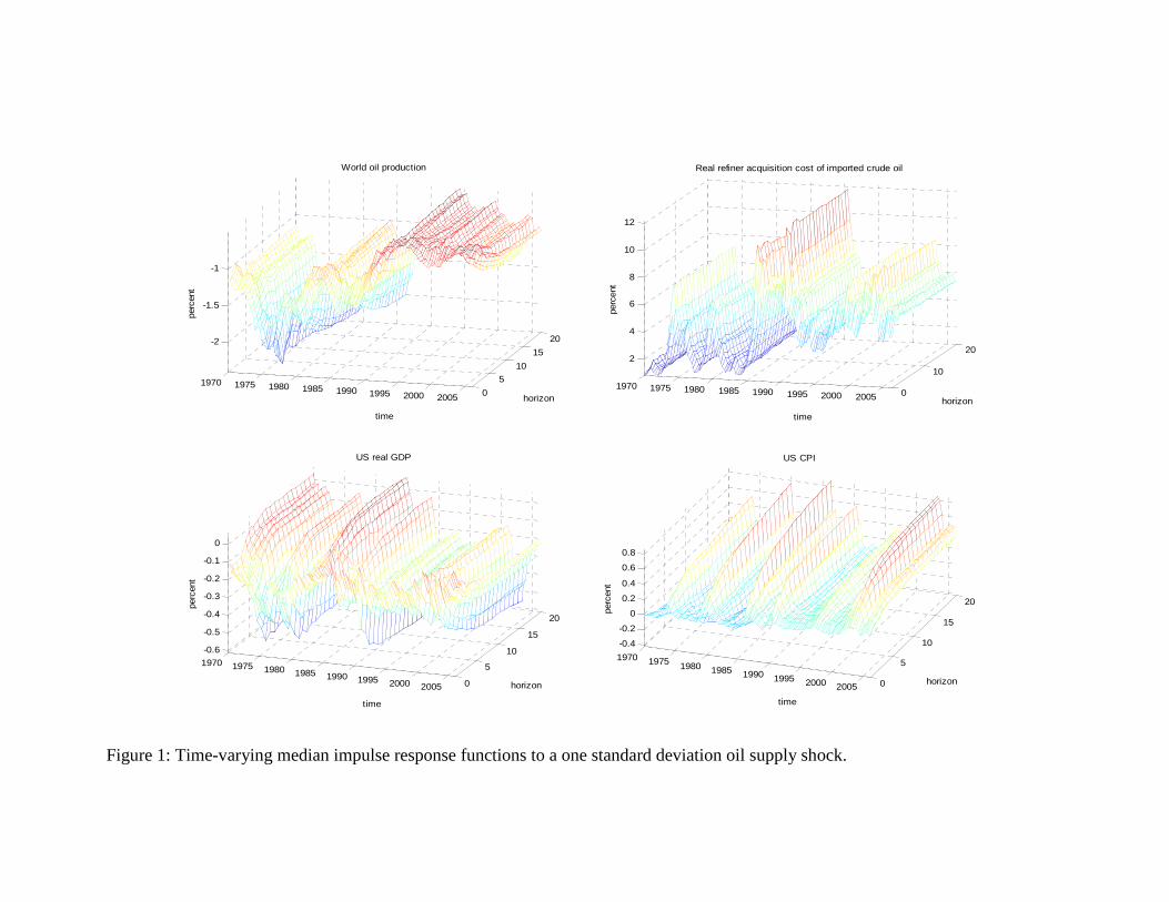
1970 1975 1980 1985 1990 1995 2000 2005 0

5

10

15

20-2

-1.5

-1

horizon

time

World oil production

perc

ent

1970 1975 1980 1985 1990 1995 2000 2005 0

10

202

4

6

8

10

12

horizon

time

Real refiner acquisition cost of imported crude oil

perc

ent

1970 1975 1980 1985 1990 1995 2000 2005 0

5

10

15

20

-0.6

-0.5

-0.4

-0.3

-0.2

-0.1

0

horizon

US real GDP

time

perc

ent

1970 1975 1980 1985 1990 1995 2000 2005 0

5

10

15

20

-0.4

-0.2

0

0.2

0.4

0.6

0.8

horizon

US CPI

time

perc

ent

Figure 1: Time-varying median impulse response functions to a one standard deviation oil supply shock.

Panel A

1970 1975 1980 1985 1990 1995 2000 2005

-3

-2

-1

0Effect of oil supply shock on QO after 4 quarters

perc

ent

1970 1975 1980 1985 1990 1995 2000 20050

5

10

15

20Effect of oil supply shock on PO after 4 quarters

perc

ent

1970 1975 1980 1985 1990 1995 2000 2005

-1

-0.5

0

0.5Effect of oil supply shock on GDP after 4 quarters

perc

ent

1970 1975 1980 1985 1990 1995 2000 2005

-0.5

0

0.5

1

Effect of oil supply shock on CPI after 4 quarters

time

perc

ent

Panel B Panel C

1970 1975 1980 1985 1990 1995 2000 20050

5

10

15

20

Effect of oil supply shock on PO after 4 quarters

perc

ent

1970 1975 1980 1985 1990 1995 2000 2005

-20

-15

-10

-5

0Effect of oil supply shock on QO after 4 quarters

perc

ent

1970 1975 1980 1985 1990 1995 2000 2005-1.5

-1

-0.5

0

0.5Effect of oil supply shock on GDP after 4 quarters

perc

ent

1970 1975 1980 1985 1990 1995 2000 2005-6

-4

-2

0

2

Effect of oil supply shock on GDP after 4 quarters

perc

ent

1970 1975 1980 1985 1990 1995 2000 2005-0.5

0

0.5

1

1.5

2Effect of oil supply shock on CPI after 4 quarters

time

perc

ent

1970 1975 1980 1985 1990 1995 2000 2005-5

-4

-3

-2

-1

0

1

2

3Effect of oil supply shock on CPI after 4 quarters

time

perc

ent

Figure 2: Median effect of an oil supply shock four quarters after the shock with 16th and 84th percentile confidence bands at each point in time. Panel A: Responses to a one standard deviation shock. Panel B: Responses after a 10% increase in the real price of oil. Panel C: Responses after a 1% shortfall in world oil production.

Figure 3: Structural changes in the global crude oil market. Panel A: Change in the volatility of oil supply shocks.

Panel B: Steeper oil demand curve.

Qoil

P2

Q2

D

Qoil

Poil Poil S2

Panel A Panel B

S1

Q1

P1

D S2 S1

P2

P1

Q2 Q1

S2'

P2'

Q2'

D'

Q2'

P2'

1970 1975 1980 1985 1990 1995 2000 20050

5

10

15

20

25

30

35

40

45Contribution of oil supply shock to variance in QO after 20 quarters

time

perc

ent

1970 1975 1980 1985 1990 1995 2000 20050

5

10

15

20

25

30

35

40

45Contribution of oil supply shock to variance in PO after 20 quarters

time

perc

ent

1970 1975 1980 1985 1990 1995 2000 20055

10

15

20

25

30

35Contribution of oil supply shock to variance in GDP after 20 quarters

time

perc

ent

1970 1975 1980 1985 1990 1995 2000 20055

10

15

20

25

30

35Contribution of oil supply shock to variance in CPI after 20 quarters

time

perc

ent

Figure 4: Contribution of oil supply shocks to the forecast error variance of all four endogenous variables (in growth rates) after 20 quarters with 16th and 84th percentiles.

1970 1975 1980 1985 1990 1995 2000 2005-2

-1

0

1

2

3

4historical decomposition of real GDP growth

baseline Y plus oil shock actual Y

1970 1975 1980 1985 1990 1995 2000 2005-1

-0.5

0

0.5

1

1.5

2

2.5

3

3.5

4historical decomposition of CPI inflation

baseline P plus oil shock actual P

1970 1975 1980 1985 1990 1995 2000 2005-40

-30

-20

-10

0

10

20

30

40historical decomposition of changes in the real price of crude oil

baseline PO plus oil shock actual PO1970 1975 1980 1985 1990 1995 2000 2005

-6

-4

-2

0

2

4

6

historical decomposition of world oil production growth

baseline QO plus oil shock actual QO

Figure 5: Historical contribution of oil supply shocks to world oil production growth, changes in the real price of crude oil, real GDP growth and CPI inflation.

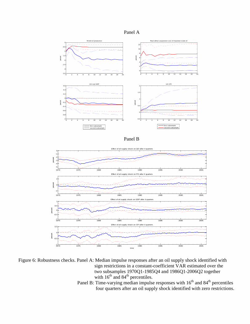
Panel A

0 2 4 6 8 10 12 14 16 18 20-3.5

-3

-2.5

-2

-1.5

-1

-0.5

0World oil production

perc

ent

0 2 4 6 8 10 12 14 16 18 20

0

2

4

6

8

10

12

Real refiner acquisition cost of imported crude oil

perc

ent

0 2 4 6 8 10 12 14 16 18 20-1

-0.8

-0.6

-0.4

-0.2

0

0.2

0.4

0.6US real GDP

perc

ent

first subsamplesecond subsample

0 2 4 6 8 10 12 14 16 18 20-0.5

0

0.5

1

1.5

2US CPI

perc

ent

first subsamplesecond subsample

Panel B

1970 1975 1980 1985 1990 1995 2000 2005

-5

-4

-3

-2

-1

0Effect of oil supply shock on QO after 4 quarters

perc

ent

1970 1975 1980 1985 1990 1995 2000 2005

-2

0

2

Effect of oil supply shock on PO after 4 quarters

perc

ent

1970 1975 1980 1985 1990 1995 2000 2005-1

-0.5

0

0.5

1Effect of oil supply shock on GDP after 4 quarters

perc

ent

1970 1975 1980 1985 1990 1995 2000 2005-1

-0.5

0

0.5Effect of oil supply shock on CPI after 4 quarters

time

perc

ent

Figure 6: Robustness checks. Panel A: Median impulse responses after an oil supply shock identified with

sign restrictions in a constant-coefficient VAR estimated over the two subsamples 1970Q1-1985Q4 and 1986Q1-2006Q2 together with 16th and 84th percentiles.

Panel B: Time-varying median impulse responses with 16th and 84th percentiles four quarters after an oil supply shock identified with zero restrictions.

Panel A

1970 1975 1980 1985 1990 1995 2000 2005 0

10

20-0.1

0

0.1

0.2

0.3

horizon

US unemployment rate

time

perc

ent

1970 1975 1980 1985 1990 1995 2000 20050

10

20

-0.5

0

0.5

horizon

time

US implicit GDP deflator

perc

ent

Panel B Panel C

1970 1975 1980 1985 1990 1995 2000 2005-2.5

-2

-1.5

-1

-0.5

0Effect of oil supply shock on QO after 4 quarters

perc

ent

1970 1975 1980 1985 1990 1995 2000 20050

5

10

15

Effect of oil supply shock on PO after 4 quarters

perc

ent

1970 1975 1980 1985 1990 1995 2000 2005-1

-0.5

0

0.5Effect of oil supply shock on GDP after 4 quarters

perc

ent

1970 1975 1980 1985 1990 1995 2000 2005

-0.5

0

0.5

1

1.5Effect of oil supply shock on CPI after 4 quarters

time

perc

ent

1970 1975 1980 1985 1990 1995 2000 2005

-3

-2

-1

0Effect of oil supply shock on QO after 4 quarters

perc

ent

1970 1975 1980 1985 1990 1995 2000 20050

5

10

15

20Effect of oil supply shock on PO after 4 quarters

perc

ent

1970 1975 1980 1985 1990 1995 2000 2005-1.5

-1

-0.5

0

0.5Effect of oil supply shock on GDP after 4 quarters

perc

ent

1970 1975 1980 1985 1990 1995 2000 2005

-0.5

0

0.5

1

1.5

Effect of oil supply shock on CPI after 4 quarters

time

perc

ent

Figure 7: Robustness checks. Panel A: Median responses of US unemployment rate (left) and US implicit GDP deflator (right) to an oil supply shock. Panel B: Median responses to an oil supply shock after 4 quarters with 16th and 84th percentiles when federal funds rate is included. Panel C: Median responses to an oil supply shock after 4 quarters with 16th and 84th percentiles when sign restrictions are imposed from t=4 to t=8.

Panel A

1.5

2

2.5

3

3.5

4

4.5

1970 19721974 1976 19781980 1982 19841986 1988 19901992 1994 19961998 2000 20022004 2006

time

thousa

nd B

TU

per

rea

l dolla

r of G

DP

Panel B

0

1

2

3

4

5

6

7

8

9

1970

Q1

1972

Q1

1974

Q1

1976

Q1

1978

Q1

1980

Q1

1982

Q1

1984

Q1

1986

Q1

1988

Q1

1990

Q1

1992

Q1

1994

Q1

1996

Q1

1998

Q1

2000

Q1

2002

Q1

2004

Q1

20

06Q1

time

per

cen

t

Figure 8: Role of oil in the US economy. Panel A: US oil intensity of production. Panel B: Share of crude oil in US total expenditures. Notes: The former has been computed as the annual petroleum consumption in British thermal units (BTU) by the industrial, commercial and part of the transportation sector per dollar of US real GDP, the latter has been calculated as number of barrels of crude oil consumed in the US economy each quarter times the nominal refiner acquisition cost of imported crude oil divided by US nominal GDP.

80

82

84

86

88

90

92

94

96

98

100

1970 1972 1974 1976 1978 1980 1982 1984 1986 1988 1990 1992 1994 1996 1998 2000 2002 2004 2006

time

per

cent

Figure 9: Global capacity utilization rates in crude oil production by year. Notes: Estimates of global spare oil production capacity are obtained from the IMF World Economic Outlook (August 2006). Spare capacity refers to production capacity that can be brought online within 30 days and sustained for 90 days. Global capacity utilization rates are calculated as percentage of total potential annual world oil production.