Embed Size (px)
Citation preview
High Gradient XFEM for
Fracture Mechanics
Von der Fakultat fur Maschinenwesen der Rheinisch-Westfalischen
Technischen Hochschule Aachen zur Erlangung des akademischen
Grades eines Doktors der Ingenieurwissenschaften genehmigte
Dissertation
vorgelegt von
Safdar Abbas
Berichter: Univ.-Prof. Marek Behr, Ph. D.
Univ.-Prof. Dr.-Ing. Stefanie Reese
Tag der mundlichen Prufung: 14.05.2012
Diese Dissertation ist auf den Internetseiten der Hochschulbibliothek online verfgbar.

2

I would like to dedicate this thesis to my loving parents especially
my late Mom. Without her prayers I wouldn’t have completed this
thesis.

Acknowledgements
First of all I thank God for helping me complete this thesis. The
first person who comes to my mind is my inspirational advisor and
mentor Dr. -Ing Thomas-Peter Fries. He was the one who hired me
and stood beside me for the whole time. His contribution to my
work has been instrumental right from the start. He is the one who
provided me with an exciting proposal to start with and he is the one
who helped me through the most difficult times during my research
by always providing constructive criticism along with motivational
guidance for the way forward. The weekly meetings were the source
of many fruitful discussions and helpful advice not only related to
work but also for personal matters. I am truly indebted and thankful
to him for all of this and much more which cannot be covered in these
few lines. I am obliged to many of my colleagues who supported me in
the XFEM research group Alaskar, Malak, Henning, Kwok and Niko.
All of you guys are responsible for creating a team environment in
the group. I would like to give special thanks to Malak for critical
technical discussions at crucial times.
My special thanks to AICES who selected me for the scholarship and
provided the best working environment for research. I would congrat-
ulate Prof. Marek Behr for founding such a great research platform
for interdisciplinary research. I would like to show my gratitude to
the AICES service team Dr. Nicole Faber, Annette de Haes, Nadine
Bachem who provided a great working environment that is a hallmark
of AICES family. I would also like to thanks all the young researchers
especially Prof. Georg May who has encouraged and supported me.
I would also like to thank Markus Bachmayr with whom I had some

very fruitful discussions. This work would not have been possible
without the financial support from the Deutsche Forschungsgemein-
schaft (German Research Association) through grant GSC 111. I am
deeply grateful for that.
I owe sincere and earnest thankfulness to my all the previous and
current room mates in AICES especially to Muhammad, Malak, Amir
and Raheel for creating a very healthy working environment. My
last year would have been very difficult without all of them. I will
keep everlasting memories of all the time we spent on campus and off
campus.
I would like to thank my loving wife Sara for her patience in her
difficult time. Her support and encouragement was critical for me
in the most challenging time of our life. Without her smile it was
difficult to get going. Special love to my sweet daughters who have
always been a source of refreshment in all these times. I am obliged
to my family and in-laws for physically and morally supporting me
throughout this time. In the end whatever I have achieved I owe it to
my father and late mother who have always prayed for my success.
Zusammenfassung
In dieser Arbeit wird ein neuer Ansatz zur Anreicherung in der erweit-
erten Finite Elemente Methode (engl.: XFEM) untersucht. Das Ziel
ist es, ein Modellkonzept bereitzustellen, in dem ein hohes Gradien-
tenfeld auf einem festen Gitter approximiert werden kann. Im Gegen-
satz zum klassischen Ansatz der Netzverfeinerung in der Nahe eines
hohen Gradienten wird ein Verfahren mit speziellen Hochgradient-
Anreicherungsfunktionen im Rahmen der XFEM vorgeschlagen. Die
Anreicherungsfunktionen sind auf Grundlage von Vorkenntnissen uber
die spezifische Eigenschaft der Hochgradient-Losung konzipiert. Das
Verfahren wird zunachst angewandt, um die steilen Gradienten in
konvektionsdominierten Problemen zu erfassen. Es werden sowohl
lineare- und nichtlineare Probleme als auch stationare und instationare
Falle betrachtet. Das Ziel dieser Arbeit ist es, das Potential dieses
Ansatzes fur Druckwellen aufzuzeigen und die allgemeinen Eigen-
schaften der XFEM fur hohen Gradienten zu untersuchen. Die Meth-
ode wird anschließend auf Problemstellungen in der Bruchmechanik
angewandt. In der klassischen XFEM sind die Rissspitzen Anre-
icherungsfunktionen abhangig von dem jeweiligen Bruchmodell. Diese
Studie zielt darauf ab, diese Modellabhangigkeit der Rissspitzen An-
reicherungsfunktionen zu beseitigen. Dieses Ziel wird durch die Wahl
eines speziellen Satzes von Hochgradient-Anreicherungsfunktionen in
der Nahe der Rissspitze erreicht, um jede große Steigung im Span-
nungsfeld zu erfassen. Die neuen Anreicherungsfunktionen werden
auf linear-elastische und kohasive Bruchmodelle in zwei und drei Di-
mensionen angewendet. Die Ergebnisse zeigen eine sehr gute Ubere-
instimmung mit den Referenzlosungen.
Abstract
In this study, a new enrichment scheme in the eXtended Finite Ele-
ment Method (XFEM) is investigated. The aim is to provide a frame-
work in which a high gradient field can be approximated on fixed
meshes. In contrast to the classical approach of mesh refinement in
the vicinity of a high gradient, an enrichment procedure with high gra-
dient enrichment functions in the context of the XFEM is proposed.
The enrichment functions are designed according to a priori knowl-
edge about the type of the high gradient solution. The method is first
applied in order to capture steep gradients in convection-dominated
problems. Linear and non-linear problems are considered as well as
stationary and instationary problems. The aim is to show the poten-
tial of this approach for shocks and to investigate the general prop-
erties of the high gradient XFEM. The method is then applied to
applications in fracture mechanics. In the classical XFEM, crack-tip
enrichment functions depend upon a particular fracture model. This
study aims at removing this model dependence of the crack-tip en-
richment functions. This aim is achieved by using a special set of high
gradient enrichment functions in the near-tip region to capture any
high gradient stress field. The new enrichment functions are applied
to linear elastic and cohesive fracture models in two and three dimen-
sions. The results show a very good agreement with the benchmark
solutions.

vi
Contents
Contents vii
List of Figures xi
Nomenclature xiv
1 Introduction 1
1.1 Background . . . . . . . . . . . . . . . . . . . . . . . . . . . . . . 1
1.2 The Present Study . . . . . . . . . . . . . . . . . . . . . . . . . . 5
1.3 Organization . . . . . . . . . . . . . . . . . . . . . . . . . . . . . 6
2 Overview of the XFEM 9
2.1 Interfaces . . . . . . . . . . . . . . . . . . . . . . . . . . . . . . . 10
2.2 Non-Smooth Fields . . . . . . . . . . . . . . . . . . . . . . . . . . 11
2.2.1 Strongly Discontinuous Field (Jumps) . . . . . . . . . . . . 11
2.2.2 Weakly Discontinuous Field (Kinks) . . . . . . . . . . . . . 12
2.2.3 High Gradient Field . . . . . . . . . . . . . . . . . . . . . 12
2.3 Level-set Method . . . . . . . . . . . . . . . . . . . . . . . . . . . 13
2.3.1 Closed Interfaces . . . . . . . . . . . . . . . . . . . . . . . 14
2.3.2 Open Interfaces . . . . . . . . . . . . . . . . . . . . . . . . 15
2.4 XFEM Formulation . . . . . . . . . . . . . . . . . . . . . . . . . . 18
2.4.1 Enrichment Functions . . . . . . . . . . . . . . . . . . . . 19
2.5 Quadrature of the Weak Form . . . . . . . . . . . . . . . . . . . . 21
2.6 Linear Dependencies and Ill-Conditioning . . . . . . . . . . . . . . 22
vii
CONTENTS
3 High Gradient XFEM 25
3.1 Convection Dominated Problems . . . . . . . . . . . . . . . . . . 25
3.1.1 Governing Equations . . . . . . . . . . . . . . . . . . . . . 26
3.1.2 Time-stepping . . . . . . . . . . . . . . . . . . . . . . . . . 27
3.1.3 Space-time Discretization . . . . . . . . . . . . . . . . . . 29
3.2 High Gradient Enrichment Functions . . . . . . . . . . . . . . . . 31
3.2.1 Classes of Regularized Step Functions . . . . . . . . . . . . 31
3.2.2 Optimal Set of Enrichment Functions . . . . . . . . . . . . 34
3.2.3 Quadrature . . . . . . . . . . . . . . . . . . . . . . . . . . 37
3.2.4 Blocking Enriched Degrees of Freedom . . . . . . . . . . . 37
3.3 Numerical Examples . . . . . . . . . . . . . . . . . . . . . . . . . 38
3.3.1 Stationary High Gradient . . . . . . . . . . . . . . . . . . 40
3.3.2 Moving High Gradient . . . . . . . . . . . . . . . . . . . . 42
3.3.3 Moving High Gradient With Unknown Position . . . . . . 43
3.3.4 Moving High Gradient in Two Dimensions . . . . . . . . . 45
3.4 Conclusions and Outlook . . . . . . . . . . . . . . . . . . . . . . . 47
4 Models in Fracture Mechanics 49
4.1 Linear Elastic Fracture . . . . . . . . . . . . . . . . . . . . . . . . 49
4.1.1 Stress Concentrations Around Flaws . . . . . . . . . . . . 49
4.1.2 Stress Based Fracture Criterion . . . . . . . . . . . . . . . 51
4.1.3 Energy Based Fracture Criterion . . . . . . . . . . . . . . 56
4.2 Elasto-Plastic Fracture . . . . . . . . . . . . . . . . . . . . . . . . 62
4.2.1 Size of the Plastic Zone . . . . . . . . . . . . . . . . . . . . 63
4.2.2 Crack Propagation Criteria . . . . . . . . . . . . . . . . . 64
4.2.2.1 Crack Tip Opening Displacement (CTOD) . . . . 64
4.2.2.2 J-Intergral . . . . . . . . . . . . . . . . . . . . . 65
4.3 Fracture Process Zone Modeling . . . . . . . . . . . . . . . . . . . 68
4.3.1 Barenblatt’s FPZ Model . . . . . . . . . . . . . . . . . . . 69
4.3.2 Dugdale’s Model . . . . . . . . . . . . . . . . . . . . . . . 70
4.3.3 Bazant’s Crack Band Model . . . . . . . . . . . . . . . . . 71
4.4 Direction of Crack Propagation . . . . . . . . . . . . . . . . . . . 71
4.4.1 Maximum Circumferential Stress . . . . . . . . . . . . . . 72
viii
CONTENTS
4.4.2 Maximum Energy Release Rate . . . . . . . . . . . . . . . 73
4.4.3 Minimum Strain Energy Density . . . . . . . . . . . . . . 74
4.5 Outlook . . . . . . . . . . . . . . . . . . . . . . . . . . . . . . . . 76
5 Numerical Fracture Mechanics 77
5.1 Hybrid Explicit-Implicit Crack Representation . . . . . . . . . . . 78
5.1.1 Explicit Crack Representation . . . . . . . . . . . . . . . . 79
5.1.2 Implicit Level-set Description . . . . . . . . . . . . . . . . 82
5.1.3 Coordinate System from Implicit Level-set Functions . . . 85
5.2 Crack Propagation . . . . . . . . . . . . . . . . . . . . . . . . . . 88
5.2.1 Maximum Hoop Stress Criterion . . . . . . . . . . . . . . . 89
5.2.2 Algorithm for the Crack Increment . . . . . . . . . . . . . 91
5.3 XFEM Formulation for Fracture Mechanics . . . . . . . . . . . . . 92
5.4 Asymptotic Crack-tip Enrichments . . . . . . . . . . . . . . . . . 95
5.5 High-Gradient Crack-tip Enrichments . . . . . . . . . . . . . . . . 98
5.5.1 Choice of the High Gradient Enrichment Functions . . . . 98
5.5.2 Optimization Procedure . . . . . . . . . . . . . . . . . . . 99
5.5.3 Edge Crack in a Square Specimen . . . . . . . . . . . . . . 101
5.5.4 Optimal Set of Enrichment Functions . . . . . . . . . . . . 102
6 Governing Equations 105
6.1 Linear Elastic Fracture . . . . . . . . . . . . . . . . . . . . . . . . 105
6.2 Cohesive Fracture . . . . . . . . . . . . . . . . . . . . . . . . . . . 107
7 Numerical Examples 113
7.1 2D Linear Elastic Fracture . . . . . . . . . . . . . . . . . . . . . . 113
7.1.1 Double Cantilever Beam . . . . . . . . . . . . . . . . . . . 113
7.1.2 Single Edge Notched Beam . . . . . . . . . . . . . . . . . . 114
7.2 2D Cohesive Fracture . . . . . . . . . . . . . . . . . . . . . . . . . 116
7.2.1 Three Point Bending Test . . . . . . . . . . . . . . . . . . 117
7.2.2 Double Cantilever Beam (Straight Crack) . . . . . . . . . 119
7.2.3 Double Cantilever Beam (Curved Crack) . . . . . . . . . . 120
7.3 3D Linear Elastic Fracture . . . . . . . . . . . . . . . . . . . . . . 121
7.3.1 Single Edge Notched Beam . . . . . . . . . . . . . . . . . . 121
ix
CONTENTS
7.3.2 Kalthoff Impact Test . . . . . . . . . . . . . . . . . . . . . 125
7.4 3D Cohesive Fracture . . . . . . . . . . . . . . . . . . . . . . . . . 127
7.4.1 Three Point Bending Test . . . . . . . . . . . . . . . . . . 127
7.4.2 Single Edge Notched Beam . . . . . . . . . . . . . . . . . . 128
8 Conclusions and Outlook 131
8.1 Conclusions . . . . . . . . . . . . . . . . . . . . . . . . . . . . . . 131
8.2 Outlook . . . . . . . . . . . . . . . . . . . . . . . . . . . . . . . . 133
References 135
x
List of Figures
2.1 Type of interfaces. . . . . . . . . . . . . . . . . . . . . . . . . . . 10
2.2 Discontinuous fields. . . . . . . . . . . . . . . . . . . . . . . . . . 11
2.3 A high gradient around a point. . . . . . . . . . . . . . . . . . . . 12
2.4 High gradient solutions. . . . . . . . . . . . . . . . . . . . . . . . 13
2.5 Level-set for closed interface. . . . . . . . . . . . . . . . . . . . . . 14
2.6 Level sets for open interfaces in 2D. . . . . . . . . . . . . . . . . . 16
2.7 Level sets for open interfaces in 3D. . . . . . . . . . . . . . . . . . 17
2.8 Element subdivisions for a curved interface. . . . . . . . . . . . . 21
2.9 Element subdivision for a hexahedron. . . . . . . . . . . . . . . . 22
2.10 Ill-Conditioning due to sub-cell division for quadrature. . . . . . . 23
3.1 Inter-element discontinuities in time-stepping. . . . . . . . . . . . 28
3.2 Space-time discretization for the discontinuous Galerkin method
in time. . . . . . . . . . . . . . . . . . . . . . . . . . . . . . . . . 29
3.3 Regularized Heaviside function for a high gradient enrichment: (a)
the gradient is scaled directly, (b) the gradient is scaled indirectly
by controlling the width. . . . . . . . . . . . . . . . . . . . . . . . 31
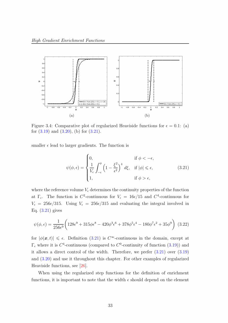
3.4 Comparative plot of regularized Heaviside functions for ǫ = 0.1:
(a) for (3.19) and (3.20), (b) for (3.21). . . . . . . . . . . . . . . . 33
3.5 Optimal sets of enrichment functions. The boxes in the left figures
show the regions which are zoomed out in the right figures. . . . . 35
3.6 Integration points in quadrilateral elements, (a) without partition-
ing, (b) with partitioning with respect to the position of the highest
gradient. . . . . . . . . . . . . . . . . . . . . . . . . . . . . . . . . 38
3.7 Results for the 1D Burgers Equation. . . . . . . . . . . . . . . . . 39
xi
LIST OF FIGURES
3.8 Convergence in the L2-norm for a diffusion coefficient of κ = 1.25 ·10−3. . . . . . . . . . . . . . . . . . . . . . . . . . . . . . . . . . . 41
3.9 Unstabilized results for the linear advection-diffusion equation in
one dimension. . . . . . . . . . . . . . . . . . . . . . . . . . . . . 42
3.10 Strong coupling loop of the Burgers equation and the transport
equation for the level-set function. . . . . . . . . . . . . . . . . . . 43
3.11 Unstabilized results for the Burgers equation. . . . . . . . . . . . 44
3.12 Unstabilized XFEM results for the linear advection-diffusion equa-
tion in two dimensions. The high-gradient solution is plotted at
the integration points in the domain. . . . . . . . . . . . . . . . . 46
4.1 Stress concentrations in solids. . . . . . . . . . . . . . . . . . . . . 50
4.2 Elliptical coordinate system. . . . . . . . . . . . . . . . . . . . . . 51
4.3 Crack-tip coordinate system. . . . . . . . . . . . . . . . . . . . . . 52
4.4 Modes of fracture. . . . . . . . . . . . . . . . . . . . . . . . . . . . 53
4.5 Penny crack. . . . . . . . . . . . . . . . . . . . . . . . . . . . . . . 58
4.6 Fixed grip condition. . . . . . . . . . . . . . . . . . . . . . . . . . 60
4.7 Fixed load condition. . . . . . . . . . . . . . . . . . . . . . . . . . 61
4.8 Load displacement condition. . . . . . . . . . . . . . . . . . . . . 62
4.9 Uniaxial nonlinear load displacement behavior [3]. . . . . . . . . . 66
4.10 Path independent J-integral. . . . . . . . . . . . . . . . . . . . . . 67
4.11 Crack tip profiles. . . . . . . . . . . . . . . . . . . . . . . . . . . . 69
4.12 Linear and nonlinear cohesive laws. . . . . . . . . . . . . . . . . . 70
4.13 Dugdale Model. . . . . . . . . . . . . . . . . . . . . . . . . . . . . 71
4.14 Crack propagation by an increment δ with angle θc. . . . . . . . . 73
5.1 . . . . . . . . . . . . . . . . . . . . . . . . . . . . . . . . . . . . . 77
5.2 Explicit crack representation in 2D. . . . . . . . . . . . . . . . . . 79
5.3 Crack tip coordinate system. . . . . . . . . . . . . . . . . . . . . . 80
5.4 3D Explicit crack in a mesh. . . . . . . . . . . . . . . . . . . . . . 81
5.5 Triangular mesh with normals. . . . . . . . . . . . . . . . . . . . . 83
5.6 Crack extension in 3D. . . . . . . . . . . . . . . . . . . . . . . . . 83
5.7 Level-set φ1. . . . . . . . . . . . . . . . . . . . . . . . . . . . . . . 84
5.8 Level-set φ2. . . . . . . . . . . . . . . . . . . . . . . . . . . . . . . 84
xii
LIST OF FIGURES
5.9 Level-set φ3 in 2D. . . . . . . . . . . . . . . . . . . . . . . . . . . 85
5.10 Iso surfaces for φ3 in 3D. . . . . . . . . . . . . . . . . . . . . . . . 86
5.11 Mesh extension in 2D. . . . . . . . . . . . . . . . . . . . . . . . . 87
5.12 r − θ coordinate system. . . . . . . . . . . . . . . . . . . . . . . . 88
5.13 a− b coordinate system. . . . . . . . . . . . . . . . . . . . . . . . 89
5.14 Stress arc around crack tip with an angle ±70. . . . . . . . . . . 90
5.15 Smooth stresses fields σθθ (red) and σrθ (blue) around a crack tip.
The direction of maximum σθθ is displayed by the thick red line
and the direction where σrθ is zero is displayed by the thick blue
line. . . . . . . . . . . . . . . . . . . . . . . . . . . . . . . . . . . 91
5.16 3D crack increment. . . . . . . . . . . . . . . . . . . . . . . . . . . 92
5.17 Nodal sets I⋆ and J⋆. . . . . . . . . . . . . . . . . . . . . . . . . . 93
5.18 Coordinates w1 and w2 (Figure taken from Cox [45]). . . . . . . . 96
5.19 Parameter c for cohesive zone. . . . . . . . . . . . . . . . . . . . . 97
5.20 Choices for the high gradient enrichment functions. . . . . . . . . 99
5.21 Edge crack test case. . . . . . . . . . . . . . . . . . . . . . . . . . 102
5.22 The optimal set of functions. . . . . . . . . . . . . . . . . . . . . . 103
5.23 High gradient enrichment function in 2D (α = 1.02). . . . . . . . . 103
6.1 Cohesionless crack. . . . . . . . . . . . . . . . . . . . . . . . . . . 105
6.2 Cohesive crack. . . . . . . . . . . . . . . . . . . . . . . . . . . . . 105
6.3 Linear cohesive law. The fracture energy Gf represents the area
under the linear law. . . . . . . . . . . . . . . . . . . . . . . . . . 108
7.1 Quasi static crack growth in a double cantilever beam. . . . . . . 114
7.2 Mesh for the double cantilever beam. . . . . . . . . . . . . . . . . 114
7.3 Comparison of the crack path. . . . . . . . . . . . . . . . . . . . . 115
7.4 Quasi static crack growth in a single edge notched beam: (a)
boundary conditions for case 1, (b) boundary conditions for case 2. 115
7.5 Mesh for the single edge notched beam: (a) case 1, (b) case 2. . . 116
7.6 Quasi static crack growth in a double cantilever beam: (a) case 1
and (b) case 2. . . . . . . . . . . . . . . . . . . . . . . . . . . . . 117
7.7 Three point bending test. . . . . . . . . . . . . . . . . . . . . . . 117
xiii
List of Figures
7.8 Load–point displacement curve for three point bending test Gf =
50N/m. . . . . . . . . . . . . . . . . . . . . . . . . . . . . . . . . 118
7.9 Load–point displacement curve for three point bending test Gf =
10N/m. . . . . . . . . . . . . . . . . . . . . . . . . . . . . . . . . 118
7.10 Double cantilever beam. . . . . . . . . . . . . . . . . . . . . . . . 119
7.11 Stress profiles. . . . . . . . . . . . . . . . . . . . . . . . . . . . . . 119
7.12 Load–point displacement curve for straight crack in a double can-
tilever beam specimen. . . . . . . . . . . . . . . . . . . . . . . . . 120
7.13 Curved crack path for double cantilever beam specimen. . . . . . 121
7.14 Load–point displacement curve for curved crack in a double can-
tilever beam specimen. . . . . . . . . . . . . . . . . . . . . . . . . 122
7.15 Quasi static crack growth in a single edge notched beam: No sup-
port on the top left side. . . . . . . . . . . . . . . . . . . . . . . . 123
7.16 Quasi static crack growth in a single edge notched beam: Support
present on the top left side. . . . . . . . . . . . . . . . . . . . . . 124
7.17 Original geometry of Kalthoff impact test. . . . . . . . . . . . . . 125
7.18 Kalthoff impact test parameters. . . . . . . . . . . . . . . . . . . . 125
7.19 Crack surface resulting from a cylindrical impact on a steel plate. 126
7.20 Three point bending test. . . . . . . . . . . . . . . . . . . . . . . 128
7.21 Load–point displacement curve for three point bending test with
Gf = 50N/m. . . . . . . . . . . . . . . . . . . . . . . . . . . . . . 129
7.22 Load–point displacement curve for three point bending test with
Gf = 10N/m. . . . . . . . . . . . . . . . . . . . . . . . . . . . . . 129
7.23 Load–point displacement curves for single edge notched beamGf =
69N/m. . . . . . . . . . . . . . . . . . . . . . . . . . . . . . . . . 130
xiv
Chapter 1
Introduction
1.1 Background
The economic impact of failures due to fracture in the US was estimated to be
around $119 billion per year by Reed et al. [118]. The cost of a failure in terms
of an injury or the loss of a life cannot be estimated. Main causes of failures
are identified as uncertainties in loading, environment, defects in materials, in-
adequacies in design and deficiencies in construction and maintenance. Fracture
mechanics deals with defects in a material. Leonardo da Vinci found out that the
strength of an iron wire is inversely proportional to the length of the wire. This
result shows that there are flaws in the material. The probability of finding flaws
in a material increases as the material volume increases. The objective of fracture
mechanics is to find the behavior of structures in the presence of initial defects
(cracks and voids) [69]. The property of a material to resist the propagation of an
initial crack is called the fracture toughness. A critical question in design is the
choice of material. A typical situation is where a designer has to select between
a material with higher yield strength but lower fracture toughness or a material
with lower yield strength and higher fracture toughness [69]. This calls for a
proper understanding of the physical phenomena effecting the fracture toughness
of a material and motivates the research in the field of fracture mechanics.
Inglis [84] performed the first systematic investigations to evaluate stress con-
centrations around sharp corners. He solved the elasticity problem of an elliptical
Introduction
hole in an otherwise uniformly loaded plate. He deduced some important results
by letting the ellipticity ratio go to zero, which is the case for a sharp crack. He
predicted an infinite stress at the tip of an extremely sharp crack. This result
means that if there is a sharp crack then the material will fail by application
of any infinitesimal load change which is in contrast to reality. This paradox
motivated Griffith [75, 76] to come up with an energy based description of frac-
ture. Griffith proposed that cracked solids have a surface energy which must be
compensated for a given crack to propagate. By formulating his theory based on
six essential elements [76], he was able to describe a measurable quantity called
the surface energy. This enabled the formulation of a mathematical expression
for the critical stress to cause a failure. Irwin [86] introduced the strain energy
release rate and denoted it by G in honor of Griffith [43]. Orowan [106] and Irwin
[87] extended the Griffith’s concept to less brittle materials. In order to consider
for the limited plastic behavior near a crack-tip, Irwin substituted the surface
energy in Griffith’s work with the plastic energy. Irwin [86, 87] later defined the
stress intensity factors K in terms of the energy release rate.
For materials exhibiting more pronounced nonlinear (plastic) behavior, the
theories of linear elastic fracture mechanics (LEFM) are not sufficient to char-
acterize the fracture behavior. In order to characterize such a plastic behavior,
two popular theories exist in the elasto-plastic fracture mechanics (EPFM) [3].
Wells [143] introduced the concept of crack-tip opening displacement (CTOD).
According to Wells, for a crack to occur there must be a critical crack opening.
In comparison to that, Rice [119, 120] adapted the concept of J-integral of Es-
helby [60, 61] for the analysis of a crack in a nonlinear material. The J-integral
can be considered as an EPFM equivalent of the energy release rate G. Rice &
Rosengren [121] showed that the J-integral can be used to characterize crack-tip
stresses and strains in nonlinear materials uniquely, where, in the absence of any
unloading, the material behaves as nonlinear elastic.
In order to circumvent some of the disadvantages of LEFM and EPFM (see
Chapter 4), the near-tip field can be modeled in terms of a fracture process zone
(FPZ). A fracture process zone is the zone around the crack-tip where important
processes take place before the complete fracture. In ductile materials, it is the
zone where voids initiate, grow and coalesce. In contrast, in cementitious materi-
2
Background
als it is the area where microcracking takes place. Barenblatt [13] introduced the
idea of a fracture process zone modeling [43] suggesting that the atomic cohesive
forces act on the inner crack zone and depend on the crack opening. Dugdale [55]
used a similar concept to model the crack-tip plastic zone. The difference is that
Barenblatt modeled the interatomic forces whereas Dugdale modeled the crack-
tip plastic deformation. Two main versions of the FPZ model used in practice
are the fictitious crack model by Hillerborg et al. [78] and the crack band model
by Bazant [16]; for details see Chapter 4.
In order to solve fracture mechanics models on computers, various numerical
methods have been utilized. The boundary element method [32, 40, 46, 79, 105]
has been a popular method for the LEFM but it has not been applied to non-
linear materials and multiple cracks [116]. Finite element methods (FEM) for
crack propagation can be divided into two categories i.e., inter-element propaga-
tion methods or intra-element propagation methods [28]. In inter-element prop-
agation methods, a crack is only allowed to propagate along the element edges
whereas in intra-element methods, a crack is allowed to propagate in any direc-
tion. Adaptive mesh refinement is often recommended in intra-element methods
[7, 49, 95, 113, 134]. The main difficulty is the transfer of internal variables from
one mesh to the other. This results in a decreased accuracy for nonlinear prob-
lems. Another problem associated with these methods is the continuous remesh-
ing which becomes cumbersome in the case of multiple cracks. The inter-element
methods are pioneered by Needleman, Ortiz and coworkers [30, 107, 151]. In these
methods, the crack growth is restricted to element edges. Special shape functions
or special interface elements called cohesive elements are used at the interface of
cracking elements. Curtin & Scher [47] and Coggan et al. [42] used the Discrete
Element Method (DEM) [90] in combination with the FEM to model cracks. In
this method the finite element mesh is adapted after every crack propagation
step.
An alternative to the mesh based finite elements is the element-free Galerkin
method (EFG) [21]. Belytschko et al. [20] applied the EFG method in the context
of crack growth in fracture mechanics. Ventura et al. [139] presented a Partition
of Unity (PU) based EFG method for the LEFM and Rabczuk & Zi [114] applied
the method to cohesive crack growth. There exist some disadvantages associated
3
Introduction
with the EFG method. Firstly, imposing essential boundary conditions is difficult
in EFG and secondly, the method is computationally very expensive as moving
least squares functions have to be evaluated at each integration point [93] and
many integration points are needed.
In enriched-mesh-based methods, the computational mesh does not conform
to the crack. Element based enrichments were realized by Dvorkin et al. [56].
This method is known as the embedded element method (EEM) or the embed-
ded discontinuity method, for an overview see [88]. A known problem with such
methods is the enforcement of the crack-path continuity [102] across the cracking
elements. Global-local finite elements [103] were used by Gifford Jr. & Hilton
[70] for fracture mechanics and by Belytschko et al. [19] for shear bands. Such
methods are computationally expensive due to the loss of sparsity of the stiffness
matrix [116]. Computational methods based on the PU concept [9, 10] avoid
mesh manipulations that are needed in most of the standard FEM based meth-
ods. Belytschko & Black [18] and Moes et al. [99] introduced a PU based method
known as the extended finite element method (XFEM) [66]. In a parallel de-
velopment, Strouboulis et al. [129, 130] introduced another PU based method
named as the generalized finite element method (GFEM). Duarte et al. [53] ap-
plied the GFEM to problems related to fracture mechanics. In both methods, the
approximation space is enriched in order to incorporate a priori knowledge of the
solution behavior into the approximation space. This is achieved by enriching the
displacement field at specified nodes. For this reason, these methods are called
nodal enrichment methods as compared to the embedded discontinuity method
which is an element enrichment method. In contrast to the EEM, there is no
need to enforce crack path continuity, that is, the crack path continues smoothly
from one element to the other. The XFEM is able to account for non-smooth fea-
tures such as discontinuities and singularities without the need for special meshes.
In one of the first applications of the XFEM, Belytschko and Black [18] used a
crack-tip enrichment function for the LEFM. The enrichment function is based
on the asymptotic field at the crack-tip for the case of brittle fracture as given by
Westergaard [146]. Moes et al. [99] added the jump enrichment function to cap-
ture the discontinuity along the crack path away from the crack-tip. The method
was successfully applied in two dimensional [27, 50, 51] and three dimensional
4
The Present Study
[73, 100, 132] elastic crack growth using LEFM theories.
One of the first applications of the XFEM to a different fracture model was
realized by Wells & Sluys [144], where the XFEM was used to simulate fracture
using the FPZ modeling (cohesive cracks). Only the generalized Heaviside func-
tion was used on a triangular mesh and no special crack-tip enrichments were
included in the formulation. As such, a sufficiently fine mesh was required to
capture the complex fields near the cohesive zone. Later, in Wells et al. [145] the
idea was extended to solve geometrically nonlinear problems. Moes & Belytschko
[98] used the XFEM to solve cohesive crack propagation problems by using a
modified crack tip enrichment. The new crack tip enrichment function was mo-
tivated by the fact that the stresses are not infinite at the crack tip for the case
of FPZ model. There are also some other interesting applications of the XFEM
to cohesive crack models, for example in [45, 94, 96, 111, 150]. However, if the
enrichment function does not represent the true asymptotic nature of the crack-
tip field, an adaptive mesh refinement must be applied to get accurate results
[1, 137].
In most of the above mentioned applications of the XFEM in fracture mechan-
ics, different crack-tip enrichment functions are used respectively for each model
in order to capture the different nature of the solution, see e.g. [97]. For someone
who needs to concentrate on modeling issues, it becomes an additional task to
design the appropriate enrichment functions. In the case where fracture models
with unknown analytical solutions are considered, a model-independent approach
is useful. In such an approach, instead of having an enrichment function based on
the asymptotic crack-tip fields, the aim is to capture all the possible solution gra-
dients in the near-tip region. This calls for a new approach where arbitrary, high
gradient solutions can be captured by appropriate enrichment functions with-
out mesh manipulations. This method is named as the High Gradient XFEM
(HG-XFEM) and is the major outcome of this disertation.
1.2 The Present Study
In the XFEM different enrichment functions are used for different kind of non-
smooth solutions. For strong discontinuities (jump in a function), the step enrich-
5
Introduction
ment function [99] is used whereas for weak discontinuities (jump in the gradient
of a function), the abs enrichment function [133] is used. For the case of con-
tinuous high gradient solutions, regularized step functions are used. Patzak &
Jirasek [111] employed regularized Heaviside functions for resolving highly local-
ized strains in narrow damage process zones of quasibrittle materials. Areias &
Belytschko [6] embedded a fine scale displacement field with a high strain gradi-
ent around a shear band. They used a tangent hyperbolic type function for the
enrichment. Benvenuti [25] also used a similar function for simulating the em-
bedded cohesive interfaces. Waisman & Belytschko [142] proposed a parametric
adaptive strategy for capturing high gradient solutions. One enrichment function
is designed to match the qualitative behavior of the exact solution with a free
parameter. The free parameter is optimized by using a-posteriori error estimates.
This work aims at developing a strategy where all the possible solution gra-
dients can be captured by a single set of enrichment functions [2]. In order to
develop this strategy one dimensional studies are performed on convection dom-
inated problems. In such problems, high gradients develop inside the domain
(shocks) and at the boundary (boundary layers). Problems are also considered
that involve moving high gradients where the advection can be linear or nonlinear
in time. For moving high gradients, an enriched space-time XFEM formulation
is used with a discontinuous Galerkin formulation in time [154]. The aim of
these preliminary studies is to investigate general properties of the proposed HG-
XFEM.
After proving the effectiveness of the HG-XFEM in the case of advection-type
problems, the same technique is applied to find model-independent enrichment
functions in fracture mechanics. A set of enrichment functions is found that
can interpolate any stress gradient in the near-tip region. The new enrichment
technique is applied to 2D and 3D problems in LEFM involving FPZ modeling
approaches.
1.3 Organization
This thesis is organized in 8 chapters. Chapter 1 motivates the need for a high
gradient XFEM for fracture mechanics. Chapter 2 provides an overview of the
6

Organization
XFEM in order to explain the basic XFEM framework. After that, in Chapter
3, a new version of the XFEM for high gradient problems is developed. In order
to develop this method, simple 1D convection dominated problems are consid-
ered. After proving the success of the method in the case of linear and non-linear
problems the focus is shifted to the main aim of this study which is to provide a
model independent XFEM-framework for fracture problems. In Chapter 4, vari-
ous fracture models are explained including crack propagation criteria. Chapter
5 provides the numerical framework for the application of the XFEM to fracture
problems. A new set of model-independent enrichment functions near the crack
tips is developed. In Chapter 6, governing equations and algorithms are provided
for applications of the XFEM to linear elastic and cohesive fracture. Chapter 7
provides numerical examples in 2D and 3D for linear elastic and cohesive fracture.
In the end, conclusions are drawn in the Chapter 8.
7

Introduction
8
Chapter 2
Overview of the XFEM
Continuum mechanics deals with the physics of continuous materials. When an
external or an internal force acts on a body, it results in a change in the body.
In order to understand a field in continuum mechanics, let us consider the ex-
ample of a displacement field. A displacement vector is defined as the vector
joining positions of a point in an undeformed and a deformed configuration. A
displacement field is defined as a vector field represented by displacement vectors
for all the points in a body. Similarly, the vector field represented by the rate of
change of displacement field is called the velocity field. Most fields of interest in a
continuum mechanics description are continuous and smooth. The finite element
method (FEM) is a numerical method for approximation of smooth fields of in-
terest. In the FEM, continuity of these fields is assumed within each element. In
some special situations, a field is non-smooth or discontinuous. This non-smooth
behavior can occur within a continuum (shocks in fluids), or across an interface
(e.g., the displacement field is non-smooth across a material interface). In these
situations, the standard FEM requires mesh manipulations which become com-
putationally very expensive in some cases. The extended finite element method
(XFEM) serves as an alternative in this case. In the XFEM, instead of manip-
ulating the computational mesh, the approximation space is enriched such that
the non-smooth solutions can be considered appropriately.
This chapter follows Fries & Belytschko [66] and gives an overview of the
XFEM in order to familiarize the reader with the basics of the XFEM. After the
classification of interfaces and description of various non-smooth fields, the level-
Overview of the XFEM
set method is explained. This method defines interfaces implicitly by means of a
scalar function in the domain. Then, the XFEM formulation is described that is
based on enriching the approximation space with suitable enrichment functions.
The non-smooth solution characteristics are included in the approximation space
by the enrichment functions. Different enrichment functions are discussed for
various non-smooth fields that are of particular interest in engineering applica-
tions. Various computational issues related to the XFEM are discussed such as
quadrature schemes for discontinuous fields and ill-conditioning of the system
matrix.
2.1 Interfaces
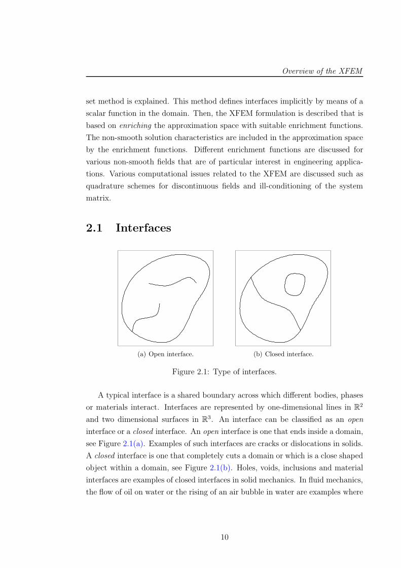
(a) Open interface. (b) Closed interface.
Figure 2.1: Type of interfaces.
A typical interface is a shared boundary across which different bodies, phases
or materials interact. Interfaces are represented by one-dimensional lines in R2
and two dimensional surfaces in R3. An interface can be classified as an open
interface or a closed interface. An open interface is one that ends inside a domain,
see Figure 2.1(a). Examples of such interfaces are cracks or dislocations in solids.
A closed interface is one that completely cuts a domain or which is a close shaped
object within a domain, see Figure 2.1(b). Holes, voids, inclusions and material
interfaces are examples of closed interfaces in solid mechanics. In fluid mechanics,
the flow of oil on water or the rising of an air bubble in water are examples where
10
Non-Smooth Fields
closed interfaces are present. In these cases, two or more phases of fluids interact.
Interfaces can also be classified in terms of a fixed interface or a moving
interface. A fixed interface is an interface whose relative position in a system
does not change. Examples of such interfaces are the material interfaces in solids
when treated by a Lagrangian description. A moving interface is an interface
whose relative position changes within a system. The rising of air bubbles in
water or the movement of water droplets in air when treated with an Eulerian
description of the fluid are examples of moving interfaces.
2.2 Non-Smooth Fields
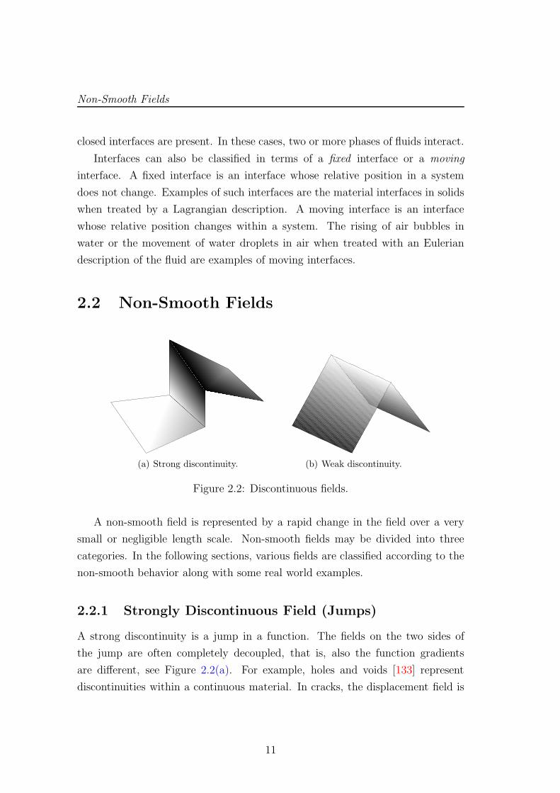
(a) Strong discontinuity. (b) Weak discontinuity.
Figure 2.2: Discontinuous fields.
A non-smooth field is represented by a rapid change in the field over a very
small or negligible length scale. Non-smooth fields may be divided into three
categories. In the following sections, various fields are classified according to the
non-smooth behavior along with some real world examples.
2.2.1 Strongly Discontinuous Field (Jumps)
A strong discontinuity is a jump in a function. The fields on the two sides of
the jump are often completely decoupled, that is, also the function gradients
are different, see Figure 2.2(a). For example, holes and voids [133] represent
discontinuities within a continuous material. In cracks, the displacement field is
11
Overview of the XFEM
discontinuous across the crack faces [99]. In shear bands [5, 6] and dislocations
[71, 140], the displacement field is discontinuous in tangential direction to the
interface. In two-phase [34, 35] or multiphase flows, there is a strong discontinuity
in the pressure field across the fluids. In fluid-structure interaction (FSI) [92, 154],
there is a strong discontinuity in the tangential velocity if a slip condition is
assumed along the fluid-structure interface.
2.2.2 Weakly Discontinuous Field (Kinks)
A weak discontinuity is a kink in a function. A field is continuous across a weak
discontinuity but its gradient is discontinuous, see Figure 2.2(b). Examples of
a weakly discontinuous field in solid mechanics is the displacement field across
a material interface [39, 63]. In two-phase flows, the velocity field is weakly
discontinuous across the fluid interface [64]. In FSI, the tangential velocity is
weakly discontinuous if no-slip conditions are assumed along the fluid-structure
interface.
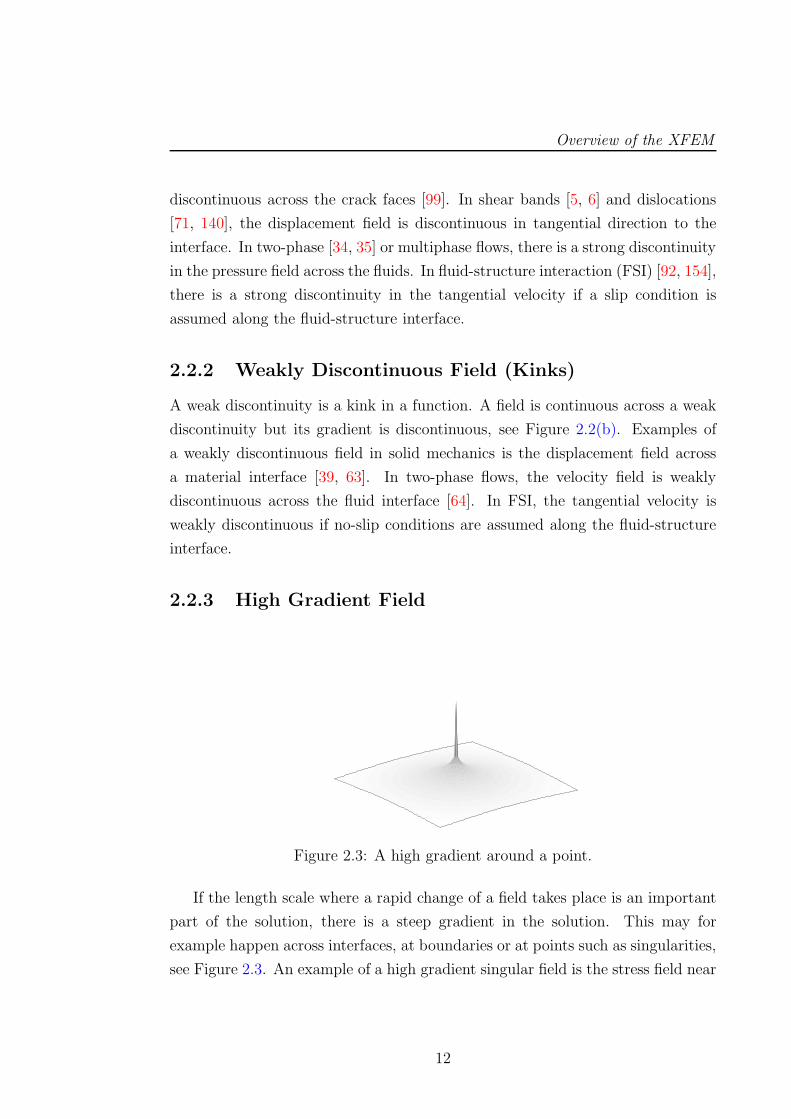
2.2.3 High Gradient Field
Figure 2.3: A high gradient around a point.
If the length scale where a rapid change of a field takes place is an important
part of the solution, there is a steep gradient in the solution. This may for
example happen across interfaces, at boundaries or at points such as singularities,
see Figure 2.3. An example of a high gradient singular field is the stress field near
12
Level-set Method
a crack tip [147]. In contrast, in the near tip region, the displacement field does
not have high gradients. In hydraulically driven fractures, the near tip pressure
field is also a high gradient field.
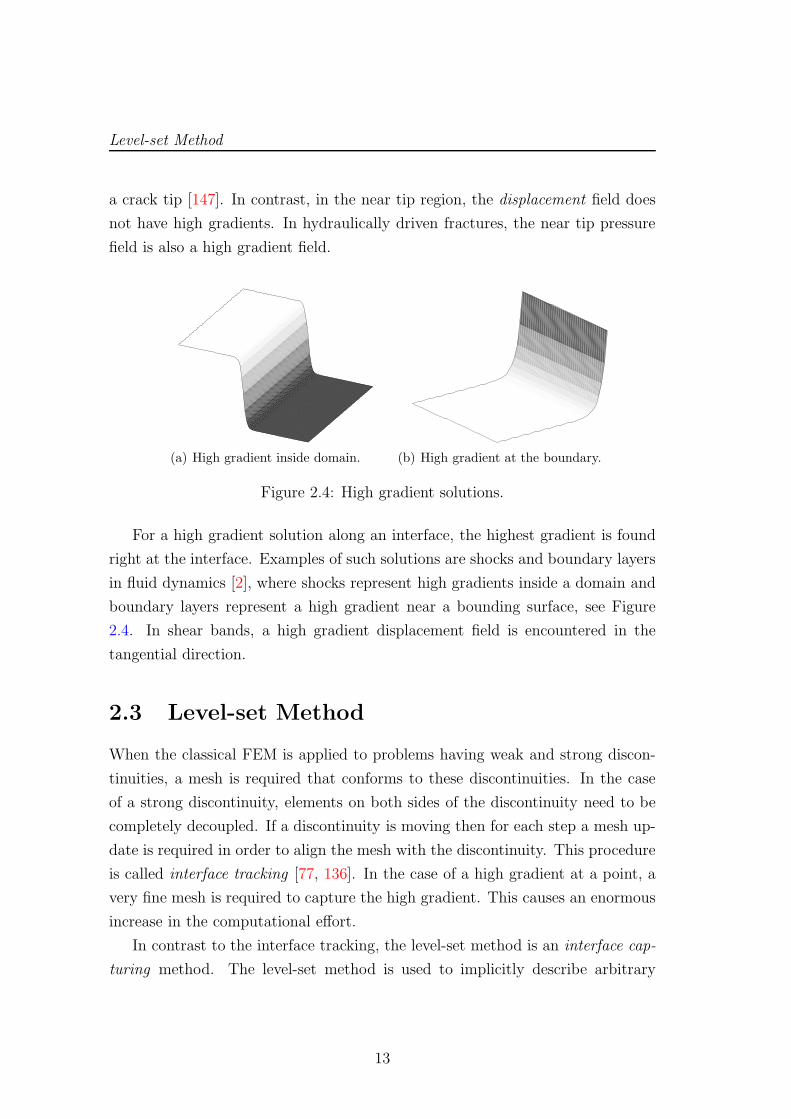
(a) High gradient inside domain. (b) High gradient at the boundary.
Figure 2.4: High gradient solutions.
For a high gradient solution along an interface, the highest gradient is found
right at the interface. Examples of such solutions are shocks and boundary layers
in fluid dynamics [2], where shocks represent high gradients inside a domain and
boundary layers represent a high gradient near a bounding surface, see Figure
2.4. In shear bands, a high gradient displacement field is encountered in the
tangential direction.
2.3 Level-set Method
When the classical FEM is applied to problems having weak and strong discon-
tinuities, a mesh is required that conforms to these discontinuities. In the case
of a strong discontinuity, elements on both sides of the discontinuity need to be
completely decoupled. If a discontinuity is moving then for each step a mesh up-
date is required in order to align the mesh with the discontinuity. This procedure
is called interface tracking [77, 136]. In the case of a high gradient at a point, a
very fine mesh is required to capture the high gradient. This causes an enormous
increase in the computational effort.
In contrast to the interface tracking, the level-set method is an interface cap-
turing method. The level-set method is used to implicitly describe arbitrary
13
Overview of the XFEM
interfaces [108, 109, 124] in domains by the zero level of a scalar function known
as the level-set function. This enables the capturing of an arbitrary interface by
a function without changing the background mesh [23, 24]. The level-set method
has become an essential ingredient for the XFEM as these methods complement
each other very well. In the XFEM, non-smooth fields are approximated by
enriching the approximation space with enrichment functions. This enrichment
procedure is applied only at places where non-smooth fields are encountered. In
a computational domain, these non-smooth fields are identified by level-set func-
tions. A level-set function also provides a natural framework for the construction
of enrichment functions, which will be explained in Section 2.4.1. Thus, in the
XFEM, a level-set function is used to define where to enrich and how to enrich.
The level-set method for capturing open and closed interfaces is discussed in the
following sections.
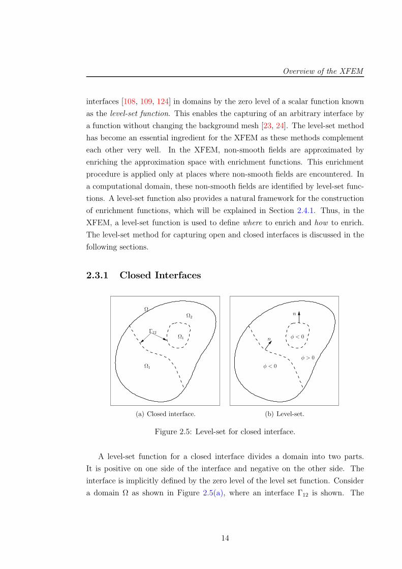
2.3.1 Closed Interfaces
Γ12
Ω1
Ω1
Ω2
Ω
(a) Closed interface.
φ < 0
φ < 0
n
φ > 0
n
(b) Level-set.
Figure 2.5: Level-set for closed interface.
A level-set function for a closed interface divides a domain into two parts.
It is positive on one side of the interface and negative on the other side. The
interface is implicitly defined by the zero level of the level set function. Consider
a domain Ω as shown in Figure 2.5(a), where an interface Γ12 is shown. The
14
Level-set Method
interface Γ12 divides the domain Ω into two parts Ω1 and Ω2. This example may
be viewed as a bimaterial problem in solid mechanics or a two phase flow problem
in fluid mechanics, where Ω1 and Ω2 represent the two materials or phases. The
interface Γ12 is defined by the zero level of a signed distance function, which is the
most commonly used level-set function. Let x ∈ Ω be an arbitrary point in the
domain, then a signed distance function φ(x) is defined as the minimum distance
from the point x to the interface Γ12
φ(x) = minx⋆∈Γ12
‖x− x⋆‖ sign(n · (x− x⋆)), (2.1)
where x⋆ is the orthogonal projection of point x on Γ12 and n is a normal to the
interface. In a discretized setting, the level set function is defined at the nodes
and is interpolated inside the elements
φh(x) =∑
i∈I
Ni(x)φi, (2.2)
where I is the number of nodes in the domain and Ni(x) are standard finite
element shape functions, used as interpolation functions.
In order to consider for the movement of an interface, the level-set function is
transported by a velocity u, i.e. the velocity of the interface with respect to the
underlying mesh. This makes the level-set function a time dependent function
φ(x, t) [35, 38]. It is updated for each time step by solving the following transport
equation∂φ
∂t+ u · ∇φ = 0 in Ω× [0, T ] , (2.3)
where T is the final time. This is a hyperbolic equation that often needs to be
stabilized in order to avoid spurious oscillations [52].
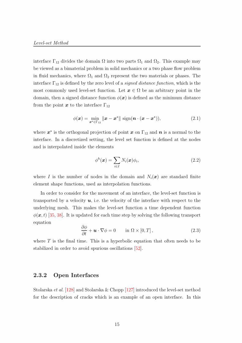
2.3.2 Open Interfaces
Stolarska et al. [128] and Stolarska & Chopp [127] introduced the level-set method
for the description of cracks which is an example of an open interface. In this
15
Overview of the XFEM
φ1 > 0
crack
φ2 > 0
φ2 < 0φ1 < 0
γ > 0
γ < 0
F
Figure 2.6: Level sets for open interfaces in 2D.
approach, a crack path is described by the zero level of a level-set function γ(x)
γ(x) = minx⋆∈Γext
cr
‖x− x⋆‖ sign(n · (x− x⋆)), (2.4)
where Γextcr is a smooth extension of the crack surface in tangential direction to
the crack and x⋆ is an orthogonal projection of an arbitrary point x on the crack
surface. This function extends in tangential direction to the crack at the crack-
tip. In order to describe a crack-tip, a second level-set φ(x) is constructed which
is orthogonal to γ(x) at the crack-tip,
φ(x) = (x− x) · t, (2.5)
where x is the position of the crack-tip and t is a tangent vector to the crack at
the crack-tip. In the case of an internal crack there are two crack-tips. In order
to describe each crack-tip a separate level-set function φi(x) may be constructed
individually, see Figure 2.6. It is convenient to describe both the tips by a single
level-set as follows:
φ(x) = maxi
(φi(x)), (2.6)
16
Level-set Method
where i is the number of crack-tips. In order to describe crack propagation, these
level-sets need to be updated for the new crack configuration. The direction of
crack propagation θ is found based on a crack propagation criterion as described in
Section 4.4. In a quasi-static crack propagation, the crack increment da is given.
Providing the information about the direction θ of the increment, an increment
vector F of the crack-tip is specified with the magnitude da. This velocity is used
to update the level-set functions γ and φ, see [128] for the details of the update
procedure.
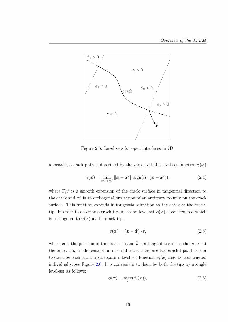
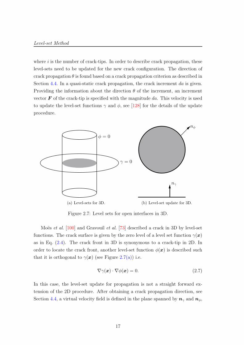
γ = 0
φ = 0
(a) Level-sets for 3D.
nφ
nγ
(b) Level-set update for 3D.
Figure 2.7: Level sets for open interfaces in 3D.
Moes et al. [100] and Gravouil et al. [73] described a crack in 3D by level-set
functions. The crack surface is given by the zero level of a level set function γ(x)
as in Eq. (2.4). The crack front in 3D is synonymous to a crack-tip in 2D. In
order to locate the crack front, another level-set function φ(x) is described such
that it is orthogonal to γ(x) (see Figure 2.7(a)) i.e.
∇γ(x) · ∇φ(x) = 0. (2.7)
In this case, the level-set update for propagation is not a straight forward ex-
tension of the 2D procedure. After obtaining a crack propagation direction, see
Section 4.4, a virtual velocity field is defined in the plane spanned by nγ and nφ,
17
Overview of the XFEM
which are normals to the zero levels of γ(x) and φ(x) respectively, see Figure
2.7(b). The velocity field is extended to the entire 3D domain by solving steady
state Hamilton-Jacobi equations as suggested by Peng et al. [112]. The level-sets
are then updated for the new crack description, see [73] for the details of the up-
date procedure. Various methods for level-set update and growth are discussed
in detail by Duflot [54].
2.4 XFEM Formulation
After the description of non-smooth fields, interfaces and the level-set method, the
XFEM formulation is now introduced. The XFEM is formulated as an extension
of the classical FE approximation. A standard XFEM approximation [18, 99] of
a scalar function uh(x) in a d-dimensional domain Ω ∈ Rd is given as
uh(x) =∑
i∈I
Ni(x)ui
︸ ︷︷ ︸
std. FE part
+∑
i∈I⋆N⋆
i (x) · ψ(x) ai︸ ︷︷ ︸
enrichment
, (2.8)
where Ni(x) are the standard FE shape functions defined at each node i ∈ I,
where I is the set of all nodes in the domain, ui are the standard FE unknowns,
N⋆i (x) are so-called “partition of unity”-functions defined only for the enriched
nodes I⋆, ψ(x) is the global enrichment function and ai are the additional un-
knowns associated with the enrichments. The functions N⋆i (x) equal Ni(x) in
this work; however this is not necessarily the case. The global enrichment func-
tion ψ(x) incorporates non-smooth solution characteristics into the approxima-
tion space. The product N⋆i (x) · ψ(x) is called the local enrichment function.
In the case of more than one enrichment term as in Section 3.2.2, the XFEM-
approximation (2.8) is extended in a straightforward manner as
uh(x) =∑
i∈I
Ni(x)ui +m∑
j=1
∑
i∈I⋆j
N⋆i (x) · ψj(x) a
ji , (2.9)
where m is the number of enrichment terms. It is noted that each enrichment
function ψj(x, t) may refer to a different set of enriched nodes I⋆j .
18
XFEM Formulation
The Kronecker-δ property that is typically present for standard FE approxi-
mation is not fulfilled for enriched approximations of the form given in Eq. (2.8)
and (2.9), i.e. uh(xi) 6= ui [22]. This renders the imposition of the essential
boundary conditions difficult. In order to recover the Kronecker-δ property of
the standard finite element approximation, the enrichment function ψ(x) has to
vanish at all the nodes. Belytschko et al. [22] proposed the following formulation
called the shifted XFEM approximation
uh(x) =∑
i∈I
Ni(x)ui +∑
i∈I⋆N⋆
i (x) · [ψ(x)− ψ(xi)] ai, (2.10)
which fulfills this property. In the rest of this work, any reference to the stan-
dard XFEM approximation, refers to the shifted approximation unless otherwise
specified.
2.4.1 Enrichment Functions
The choice of the global enrichment function ψ(x) is critical for an XFEM applica-
tion. An enrichment function incorporates the knowledge about the local solution
behavior into the approximation space. This function represents the true nature
of the solution behavior in a localized zone. In this section, enrichment functions
for weak and strong discontinuities are discussed. Enrichment functions for high
gradient solutions are discussed in Chapter 3, whereas enrichment functions for
crack-tips are discussed in Chapter 5.
As discussed earlier, a strong discontinuity is characterized by a jump in a
function. In order to include this solution knowledge into the approximation
space, a step function is used as an enrichment function in the case of a strong
discontinuity. Two commonly used step functions are the Heaviside function or
the sign function. These functions can be built from the signed distance function
as follows
Heaviside enrichment: ψ(x) = H(φ(x)) =
0 : φ(x) 6 0,
1 : φ(x) > 0.(2.11)
19
Overview of the XFEM
Sign enrichment: ψ(x) = Sign(φ(x)) =
−1 : φ(x) < 0,
0 : φ(x) = 0,
1 : φ(x) > 0.
(2.12)
Any of these functions can be used for enriching a strongly discontinuous field
as both of these functions span the same approximation space. In the case of
a discontinuity along open interfaces, the tip of the discontinuity lies inside the
domain, e.g. in the case of cracks, dislocations and shear bands. At the tip, one
typically encounters high gradients such as singularities. Then, in addition to the
step enrichment, further enrichment functions are used in this case to capture the
steep gradients which will be discussed in detail in Chapter 5.
Weak discontinuities are characterized by kinks in a function. Such disconti-
nuities can be captured by enriching the approximation field with functions that
have kinks. One of the simplest approaches is the abs enrichment [22, 133]. This
can be built from a signed distance function by taking its absolute value
ψ(x) = abs(φ(x)) = |φ(x)|. (2.13)
The local enrichment N⋆i · ψ(x) results in three kinds of elements: (i) the
elements with none of the nodes enriched are called standard finite elements, (ii)
the elements for which all the nodes are enriched are called reproducing elements,
and (iii) the elements for which some of the nodes are enriched are called blending
elements. There are some special issues associated with blending elements in the
XFEM. These issues are important when enrichment functions are neither zero
nor constant in the blending elements (as is, for example, the case for the abs-
enrichment (2.13)). Enrichment functions used in this work are mostly constant
in the blending elements so a detailed discussion on this issue is out of the scope
of this work. Details of problems in blending elements and their solution can be
found in [63, 72, 133, 141].
20
Quadrature of the Weak Form
Interface
(a) A curved interface pass-ing through a quadrilateral el-ement.
Interface
(b) Subdivision into polygons. (c) Subdivision into trianglesand quadrilaterals.
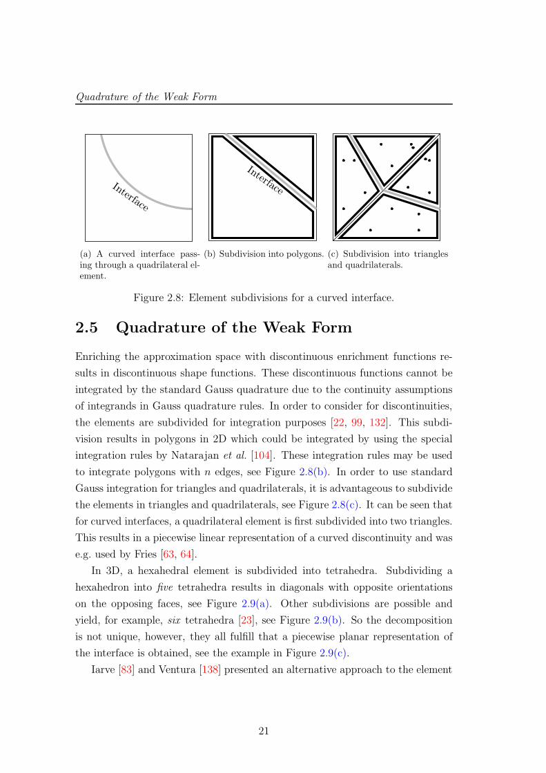
Figure 2.8: Element subdivisions for a curved interface.
2.5 Quadrature of the Weak Form
Enriching the approximation space with discontinuous enrichment functions re-
sults in discontinuous shape functions. These discontinuous functions cannot be
integrated by the standard Gauss quadrature due to the continuity assumptions
of integrands in Gauss quadrature rules. In order to consider for discontinuities,
the elements are subdivided for integration purposes [22, 99, 132]. This subdi-
vision results in polygons in 2D which could be integrated by using the special
integration rules by Natarajan et al. [104]. These integration rules may be used
to integrate polygons with n edges, see Figure 2.8(b). In order to use standard
Gauss integration for triangles and quadrilaterals, it is advantageous to subdivide
the elements in triangles and quadrilaterals, see Figure 2.8(c). It can be seen that
for curved interfaces, a quadrilateral element is first subdivided into two triangles.
This results in a piecewise linear representation of a curved discontinuity and was
e.g. used by Fries [63, 64].
In 3D, a hexahedral element is subdivided into tetrahedra. Subdividing a
hexahedron into five tetrahedra results in diagonals with opposite orientations
on the opposing faces, see Figure 2.9(a). Other subdivisions are possible and
yield, for example, six tetrahedra [23], see Figure 2.9(b). So the decomposition
is not unique, however, they all fulfill that a piecewise planar representation of
the interface is obtained, see the example in Figure 2.9(c).
Iarve [83] and Ventura [138] presented an alternative approach to the element
21
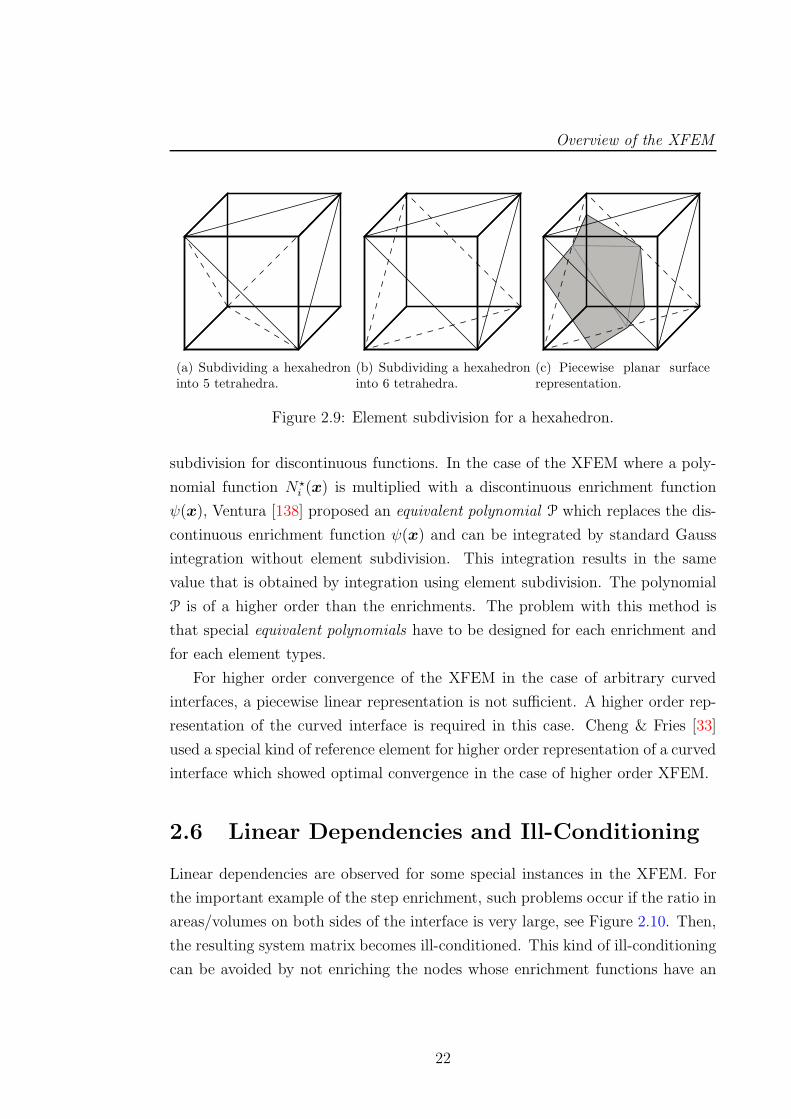
Overview of the XFEM
(a) Subdividing a hexahedroninto 5 tetrahedra.
(b) Subdividing a hexahedroninto 6 tetrahedra.
(c) Piecewise planar surfacerepresentation.
Figure 2.9: Element subdivision for a hexahedron.
subdivision for discontinuous functions. In the case of the XFEM where a poly-
nomial function N⋆i (x) is multiplied with a discontinuous enrichment function
ψ(x), Ventura [138] proposed an equivalent polynomial P which replaces the dis-
continuous enrichment function ψ(x) and can be integrated by standard Gauss
integration without element subdivision. This integration results in the same
value that is obtained by integration using element subdivision. The polynomial
P is of a higher order than the enrichments. The problem with this method is
that special equivalent polynomials have to be designed for each enrichment and
for each element types.
For higher order convergence of the XFEM in the case of arbitrary curved
interfaces, a piecewise linear representation is not sufficient. A higher order rep-
resentation of the curved interface is required in this case. Cheng & Fries [33]
used a special kind of reference element for higher order representation of a curved
interface which showed optimal convergence in the case of higher order XFEM.
2.6 Linear Dependencies and Ill-Conditioning
Linear dependencies are observed for some special instances in the XFEM. For
the important example of the step enrichment, such problems occur if the ratio in
areas/volumes on both sides of the interface is very large, see Figure 2.10. Then,
the resulting system matrix becomes ill-conditioned. This kind of ill-conditioning
can be avoided by not enriching the nodes whose enrichment functions have an
22
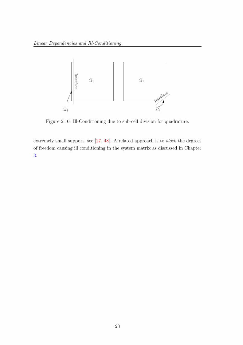
Linear Dependencies and Ill-Conditioning
Ω2
Interface
Interface
Ω1 Ω1
Ω2
Figure 2.10: Ill-Conditioning due to sub-cell division for quadrature.
extremely small support, see [27, 48]. A related approach is to block the degrees
of freedom causing ill conditioning in the system matrix as discussed in Chapter
3.
23

Overview of the XFEM
24
Chapter 3
High Gradient XFEM
In this chapter a new enrichment scheme in the XFEM is introduced with the
aim to capture arbitrary, steep gradients in solution fields. This new high gradi-
ent XFEM (HG-XFEM) is applied to advection dominated problems where the
steep gradients occur across close interfaces as shall be seen below. This chap-
ter presents a systematic approach for the development of suitable enrichment
functions and investigates general properties of the HG-XFEM. In subsequent
chapters, the HG-XFEM is adapted for applications in fracture mechanics where
the steep gradients are expected at the tip/front of open interfaces.
3.1 Convection Dominated Problems
The problems under consideration here consist of two mechanisms: convection
and diffusion. High solution gradients develop due to the domination of con-
vection. In convection-diffusion problems, the diffusion operator is a symmetric
Laplace operator that is given by divergence of the gradient of a function. In
contrast convection operator is a non-symmetric operator, represented by veloc-
ity times the divergence of a field. In the case of a symmetric operator, the
Galerkin method possesses the best approximation property, which means that
the difference between the FEM solution and the exact solution is minimized
with respect to a certain norm [29]. This property is lost in the case of the non-
symmetric convection operator which results in spurious node-to-node oscillations
High Gradient XFEM
in the solution [52]. In the standard FEM, these oscillations are eliminated by
mesh refinement and/or stabilization techniques [29, 80, 135]. In this chapter, a
computational method is devised that avoids stabilization and mesh refinement
yielding high quality representations of high gradient solutions1.
3.1.1 Governing Equations
In this chapter the linear advection-diffusion equation and the Burgers equation
are considered as model problems for convection dominated affects. In this sec-
tion, the governing equations for the two model problems are described. Let Ω
be an open, bounded region in Ω ∈ Rd. The boundary is denoted by Γ and is as-
sumed smooth. The linear advection-diffusion equation with prescribed constant
velocities c ∈ Rd and a constant, scalar diffusion parameter κ ∈ R is stated in the
following initial/boundary value problem: Find u(x, t) ∀x ∈ Ω and ∀t ∈ [0, T ]
such that
u(x, t) = −c · ∇u+ κ ·∆u, in Ω × ]0, T [, (3.1)
u(x, 0) = u0(x), ∀x ∈ Ω (3.2)
u(x, t) = u(x, t), ∀x ∈ Γ × ]0, T [, (3.3)
whereas the Burgers equation is given as: Find u(x, t) ∀x ∈ Ω and ∀t ∈ [0, T ]
such that
u(x, t) = −u · ∇u+ κ ·∆u, in Ω × ]0, T [, (3.4)
u(x, 0) = u0(x), ∀x ∈ Ω (3.5)
u(x, t) = u(x, t), ∀x ∈ Γ × ]0, T [. (3.6)
where ∆u = ∇ · (∇u) and u = ∂u/∂t. The initial condition u0 : Ω → R and
Dirichlet boundary condition u : Γ×]0, T [→ R are prescribed data. No Neumann
boundary conditions are considered. These equations involve spacial and time
dependent terms. Spacial discretization is given by the standard XFEM approx-
imation (2.10). Two different schemes are used for the temporal discretization.
1Most of the paragraphs in this chapter are taken from the author’s own publication [2].
26
Convection Dominated Problems
These schemes are described in the following sections.
3.1.2 Time-stepping
The first scheme for the temporal discretization is time-stepping. In the case of
moving interfaces, application of time-stepping schemes requires special attention
in the context of the XFEM [36, 37, 67]. For the approximation with finite
elements, the problem has to be stated in its discretized variational form. The
variational form also depends on the time-discretization: If the derivative in time
is treated by finite differences the trial and test function spaces are
ShTS =
uh ∈ H1h(Ω) | uh = uh on Γ
, (3.7)
VhTS =
wh ∈ H1h(Ω) | wh = 0 on Γ
, (3.8)
where “TS” stands for “time stepping”. H1h is a finite dimensional subspace of
the space of square-integrable functions with square-integrable first derivatives.
H1h is spanned by the standard finite element and enrichment functions given
in the approximation (2.10). Using the Trapezoidal rule for time stepping, the
discretized weak forms for equations (3.1) and (3.4) are described as
1
t
∫
Ω
wh(uhn+1 − uhn)dΩ+1
2
∫
Ω
c wh · ((uhn+1),x + (uhn),x)
+1
2
∫
Ω
kwh,x · ((uhn+1),x + (uhn),x) = 0,
(3.9)
and
1
t
∫
Ω
wh(uhn+1 − uhn)dΩ+1
2
∫
Ω
wh · un+1 · (uhn+1),x +1
2
∫
Ω
wh · un · (uhn),x
+1
2
∫
Ω
kwh,x · ((uhn+1),x + (uhn),x) = 0,
(3.10)
respectively, where uh ∈ STS such that ∀wh ∈ VTS. un is the solution in the
current time step, un+1 is the solution at the next time step and t is the size
of the time-step. Due to the temporal dependence of the shape functions, semi-
discrete methods explained in Donea & Huerta [52], cannot be applied in this case,
27
High Gradient XFEM
0
Ω3Ω1 Ω2
t
x⋆n x⋆n+1
x
tn
tn+1
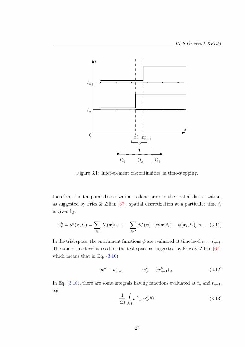
Figure 3.1: Inter-element discontinuities in time-stepping.
therefore, the temporal discretization is done prior to the spatial discretization,
as suggested by Fries & Zilian [67]. spatial discretization at a particular time tr
is given by:
uhr = uh(x, tr) =∑
i∈I
Ni(x)ui +∑
i∈I⋆N⋆
i (x) · [ψ(x, tr)− ψ(xi, tr)] ai. (3.11)
In the trial space, the enrichment functions ψ are evaluated at time level tr = tn+1.
The same time level is used for the test space as suggested by Fries & Zilian [67],
which means that in Eq. (3.10)
wh = whn+1 wh
,x = (whn+1),x. (3.12)
In Eq. (3.10), there are some integrals having functions evaluated at tn and tn+1,
e.g.1
t
∫
Ω
whn+1u
hndΩ. (3.13)
28
Convection Dominated Problems
In this case, the enrichment functions are evaluated at each time level. This
results in different positions of high gradient in the spatial domain, see Figure
3.1. Elements are subdivided into sub-cells for integration purposes, as described
in Section 3.2.3, taking into account both positions of high gradient in each time
step.
3.1.3 Space-time Discretization
Time−slab
Position of thehighest gradient
t−n
t
x
tn+1
t+n
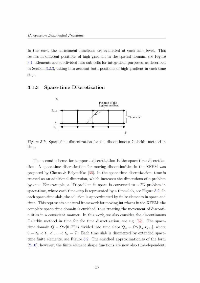
Figure 3.2: Space-time discretization for the discontinuous Galerkin method intime.
The second scheme for temporal discretization is the space-time discretiza-
tion. A space-time discretization for moving discontinuities in the XFEM was
proposed by Chessa & Belytschko [36]. In the space-time discretization, time is
treated as an additional dimension, which increases the dimensions of a problem
by one. For example, a 1D problem in space is converted to a 2D problem in
space-time, where each time-step is represented by a time-slab, see Figure 3.2. In
each space-time slab, the solution is approximated by finite elements in space and
time. This represents a natural framework for moving interfaces in the XFEM: the
complete space-time domain is enriched, thus treating the movement of disconti-
nuities in a consistent manner. In this work, we also consider the discontinuous
Galerkin method in time for the time discretization, see e.g. [52]. The space-
time domain Q = Ω×]0, T [ is divided into time slabs Qn = Ω×]tn, tn+1[, where
0 = t0 < t1 < . . . < tN = T . Each time slab is discretized by extended space-
time finite elements, see Figure 3.2. The enriched approximation is of the form
(2.10), however, the finite element shape functions are now also time-dependent,
29
High Gradient XFEM
i.e. Ni(x, t) and N⋆i (x, t). The test and trial function spaces are
ShST =
uh ∈ H1h(Qn) | uh = uh on Γ×]tn, tn+1[
, (3.14)
VhST =
wh ∈ H1h(Qn) | wh = 0 on Γ×]tn, tn+1[
, (3.15)
and are again spanned by the FE shape functions and enrichment functions in
Eq. (2.10). “ST” stands for “space-time”.
The discretized weak form for equations (3.1) and (3.4) are given as
∫
Qn
wh ·(uh,t + cuh,x
)dQ+
∫
Qn
kwh,x · uh,x
+
∫
Ωn
(wh
)+
n·((uh
)+
n−
(uh
)−n
)
dΩ = 0,
(3.16)
and
∫
Qn
wh · uh,t dQ+
∫
Qn
wh · uh(x, t) · uh,x dQ
+
∫
Qn
kwh,x · uh,x dQ+
∫
Ωn
(wh
)+
n·((uh
)+
n−(uh
)−n
)
dΩ = 0,
(3.17)
respectively, where uh ∈ ShST such that ∀wh ∈ V
hST ,
(uh
)−nis given and
(uh
)±nis
defined as(uh
)±n= lim
ε→0uh (x, tn ± ε) . (3.18)
The continuity of the field variables is weakly enforced across the time-slabs
i.e.∫
Ωn
(wh
)+
n·((uh
)+
n−
(uh
)−n
)
dΩ. The initial condition uh0 is set to(uh
)−0.
Convergence properties of the space-time formulation for the XFEM were
investigated by Fries & Zilian [67] for linear elements, and by Cheng & Fries
[33] for higher order XFEM. Optimal order of convergence rates were obtained
but the method is computationally twice as expensive, e.g. 3D problems in space
require a 4D space-time domain. Such an application has not yet been published
for the XFEM. Chessa & Belytschko [37] suggested a hybrid method where the
space-time XFEM is used only in elements where discontinuities exist. For the
rest of the domain, time-stepping is used.
30
High Gradient Enrichment Functions
1
m
x
ψ
(a)
ψ
x−ǫ +ǫ
(b)
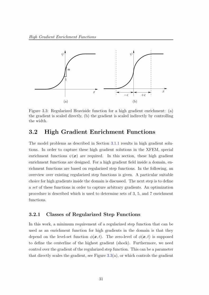
Figure 3.3: Regularized Heaviside function for a high gradient enrichment: (a)the gradient is scaled directly, (b) the gradient is scaled indirectly by controllingthe width.
3.2 High Gradient Enrichment Functions
The model problems as described in Section 3.1.1 results in high gradient solu-
tions. In order to capture these high gradient solutions in the XFEM, special
enrichment functions ψ(x) are required. In this section, these high gradient
enrichment functions are designed. For a high gradient field inside a domain, en-
richment functions are based on regularized step functions. In the following, an
overview over existing regularized step functions is given. A particular suitable
choice for high gradients inside the domain is discussed. The next step is to define
a set of these functions in order to capture arbitrary gradients. An optimization
procedure is described which is used to determine sets of 3, 5, and 7 enrichment
functions.
3.2.1 Classes of Regularized Step Functions
In this work, a minimum requirement of a regularized step function that can be
used as an enrichment function for high gradients in the domain is that they
depend on the level-set function φ(x, t). The zero-level of φ(x, t) is supposed
to define the centerline of the highest gradient (shock). Furthermore, we need
control over the gradient of the regularized step function. This can be a parameter
that directly scales the gradient, see Figure 3.3(a), or which controls the gradient
31
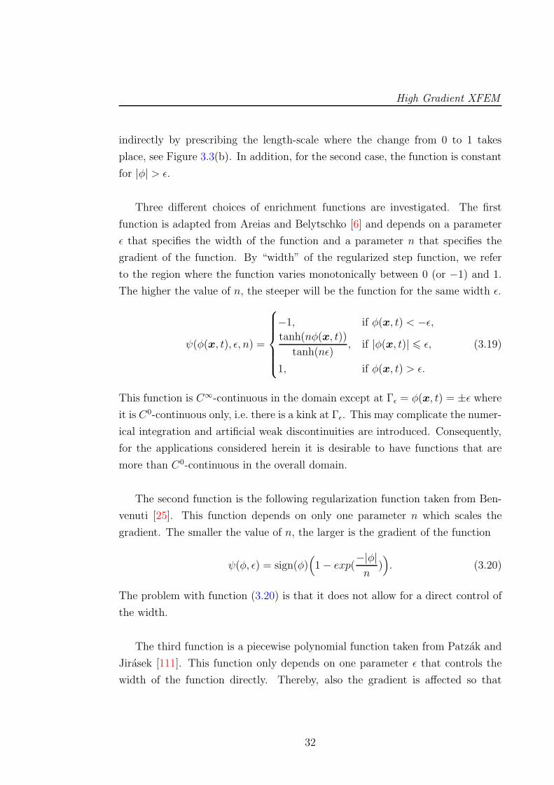
High Gradient XFEM
indirectly by prescribing the length-scale where the change from 0 to 1 takes
place, see Figure 3.3(b). In addition, for the second case, the function is constant
for |φ| > ǫ.
Three different choices of enrichment functions are investigated. The first
function is adapted from Areias and Belytschko [6] and depends on a parameter
ǫ that specifies the width of the function and a parameter n that specifies the
gradient of the function. By “width” of the regularized step function, we refer
to the region where the function varies monotonically between 0 (or −1) and 1.
The higher the value of n, the steeper will be the function for the same width ǫ.
ψ(φ(x, t), ǫ, n) =
−1, if φ(x, t) < −ǫ,tanh(nφ(x, t))
tanh(nǫ), if |φ(x, t)| 6 ǫ,
1, if φ(x, t) > ǫ.
(3.19)
This function is C∞-continuous in the domain except at Γǫ = φ(x, t) = ±ǫ whereit is C0-continuous only, i.e. there is a kink at Γǫ. This may complicate the numer-
ical integration and artificial weak discontinuities are introduced. Consequently,
for the applications considered herein it is desirable to have functions that are
more than C0-continuous in the overall domain.
The second function is the following regularization function taken from Ben-
venuti [25]. This function depends on only one parameter n which scales the
gradient. The smaller the value of n, the larger is the gradient of the function
ψ(φ, ǫ) = sign(φ)(
1− exp(−|φ|n
))
. (3.20)
The problem with function (3.20) is that it does not allow for a direct control of
the width.
The third function is a piecewise polynomial function taken from Patzak and
Jirasek [111]. This function only depends on one parameter ǫ that controls the
width of the function directly. Thereby, also the gradient is affected so that
32
High Gradient Enrichment Functions
−1 −0.8 −0.6 −0.4 −0.2 0 0.2 0.4 0.6 0.8 1
−1
−0.8
−0.6
−0.4
−0.2
0
0.2
0.4
0.6
0.8
1
−ε ε
φ
ψ
Enr. Func.(23), ε = 0.1, n = 20Enr. Func.(24), ε = 0.1
(a)
−1 −0.8 −0.6 −0.4 −0.2 0 0.2 0.4 0.6 0.8 1
0
0.2
0.4
0.6
0.8
1
−ε ε
φ
ψ
Enr. Func.(25), ε = 0.1
(b)
Figure 3.4: Comparative plot of regularized Heaviside functions for ǫ = 0.1: (a)for (3.19) and (3.20), (b) for (3.21).
smaller ǫ lead to larger gradients. The function is
ψ(φ, ǫ) =
0, if φ < −ǫ,1
Vǫ
∫ φ
−ǫ
(
1− ξ2
ǫ2
)4
dξ, if |φ| 6 ǫ,
1, if φ > ǫ,
(3.21)
where the reference volume Vǫ determines the continuity properties of the function
at Γǫ. The function is C2-continuous for Vǫ = 16ǫ/15 and C4-continuous for
Vǫ = 256ǫ/315. Using Vǫ = 256ǫ/315 and evaluating the integral involved in
Eq. (3.21) gives
ψ(φ, ǫ) =1
256ǫ9
(
128ǫ9 + 315φǫ8 − 420φ3ǫ6 + 378φ5ǫ4 − 180φ7ǫ2 + 35φ9
)
(3.22)
for |φ(x, t)| 6 ǫ. Definition (3.21) is C∞-continuous in the domain, except at
Γǫ where it is C4-continuous (compared to C0-continuity of function (3.19)) and
it allows a direct control of the width. Therefore, we prefer (3.21) over (3.19)
and (3.20) and use it throughout this chapter. For other examples of regularized
Heaviside functions, see [26].
When using the regularized step functions for the definition of enrichment
functions, it is important to note that the width ǫ should depend on the element
33
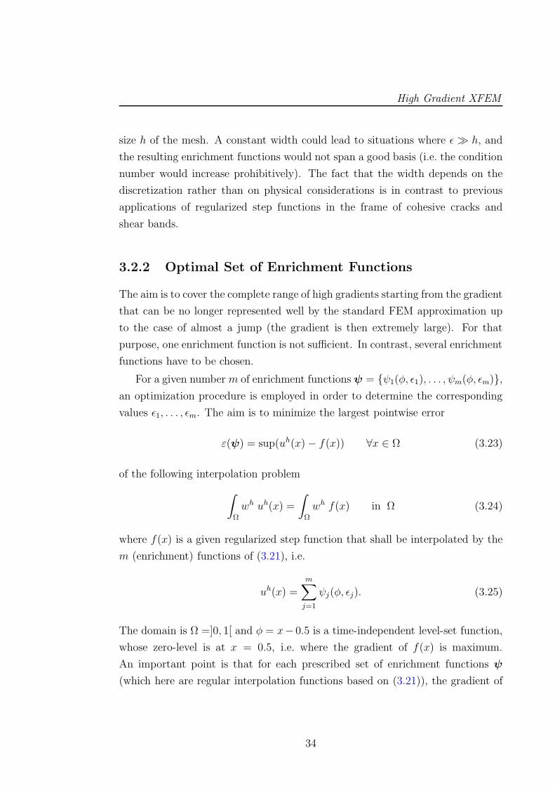
High Gradient XFEM
size h of the mesh. A constant width could lead to situations where ǫ ≫ h, and
the resulting enrichment functions would not span a good basis (i.e. the condition
number would increase prohibitively). The fact that the width depends on the
discretization rather than on physical considerations is in contrast to previous
applications of regularized step functions in the frame of cohesive cracks and
shear bands.
3.2.2 Optimal Set of Enrichment Functions
The aim is to cover the complete range of high gradients starting from the gradient
that can be no longer represented well by the standard FEM approximation up
to the case of almost a jump (the gradient is then extremely large). For that
purpose, one enrichment function is not sufficient. In contrast, several enrichment
functions have to be chosen.
For a given number m of enrichment functions ψ = ψ1(φ, ǫ1), . . . , ψm(φ, ǫm),an optimization procedure is employed in order to determine the corresponding
values ǫ1, . . . , ǫm. The aim is to minimize the largest pointwise error
ε(ψ) = sup(uh(x)− f(x)) ∀x ∈ Ω (3.23)
of the following interpolation problem
∫
Ω
wh uh(x) =
∫
Ω
wh f(x) in Ω (3.24)
where f(x) is a given regularized step function that shall be interpolated by the
m (enrichment) functions of (3.21), i.e.
uh(x) =m∑
j=1
ψj(φ, ǫj). (3.25)
The domain is Ω =]0, 1[ and φ = x− 0.5 is a time-independent level-set function,
whose zero-level is at x = 0.5, i.e. where the gradient of f(x) is maximum.
An important point is that for each prescribed set of enrichment functions ψ
(which here are regular interpolation functions based on (3.21)), the gradient of
34
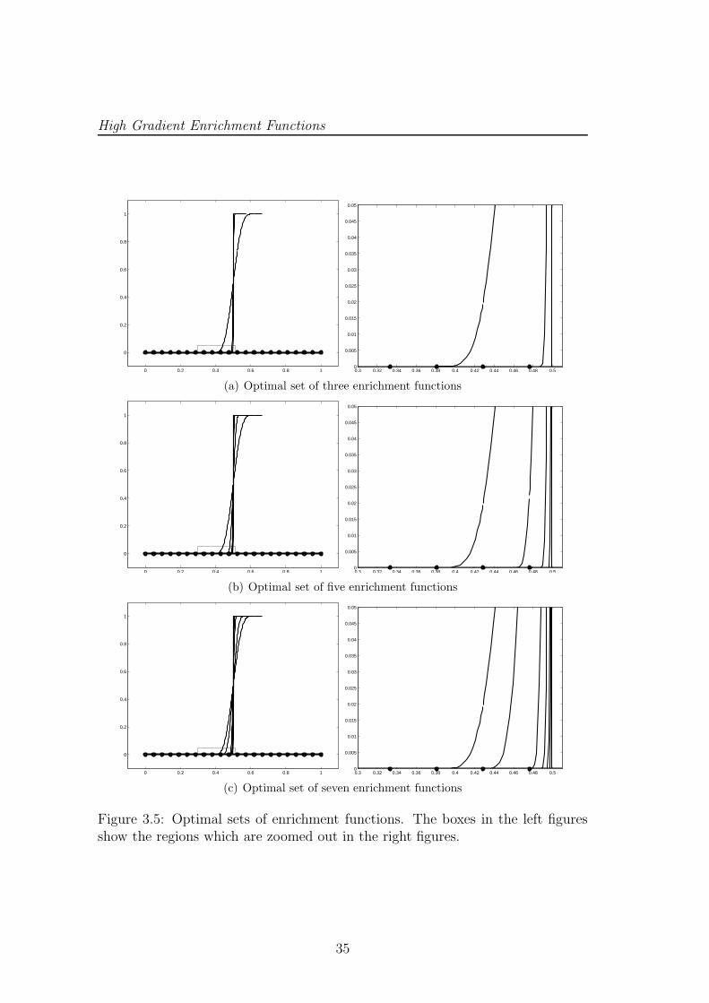
High Gradient Enrichment Functions
0 0.2 0.4 0.6 0.8 1
0
0.2
0.4
0.6
0.8
1
0.3 0.32 0.34 0.36 0.38 0.4 0.42 0.44 0.46 0.48 0.50
0.005
0.01
0.015
0.02
0.025
0.03
0.035
0.04
0.045
0.05
(a) Optimal set of three enrichment functions
0 0.2 0.4 0.6 0.8 1
0
0.2
0.4
0.6
0.8
1
0.3 0.32 0.34 0.36 0.38 0.4 0.42 0.44 0.46 0.48 0.50
0.005
0.01
0.015
0.02
0.025
0.03
0.035
0.04
0.045
0.05
(b) Optimal set of five enrichment functions
0 0.2 0.4 0.6 0.8 1
0
0.2
0.4
0.6
0.8
1
0.3 0.32 0.34 0.36 0.38 0.4 0.42 0.44 0.46 0.48 0.50
0.005
0.01
0.015
0.02
0.025
0.03
0.035
0.04
0.045
0.05
(c) Optimal set of seven enrichment functions
Figure 3.5: Optimal sets of enrichment functions. The boxes in the left figuresshow the regions which are zoomed out in the right figures.
35
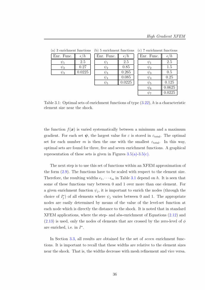
High Gradient XFEM
(a) 3 enrichment functions
Enr. Func. ǫ/h
ψ1 2.5ψ2 0.27ψ3 0.0225
(b) 5 enrichment functions
Enr. Func. ǫ/h
ψ1 2.5ψ2 0.85ψ3 0.265ψ4 0.085ψ5 0.0225
(c) 7 enrichment functions
Enr. Func. ǫ/h
ψ1 2.5ψ2 1.5ψ3 0.5ψ4 0.25ψ5 0.125ψ6 0.0625ψ7 0.0225
Table 3.1: Optimal sets of enrichment functions of type (3.22), h is a characteristicelement size near the shock.
the function f(x) is varied systematically between a minimum and a maximum
gradient. For each set ψ, the largest value for ε is stored in εtotal. The optimal
set for each number m is then the one with the smallest εtotal. In this way,
optimal sets are found for three, five and seven enrichment functions. A graphical
representation of these sets is given in Figures 3.5(a)-3.5(c).
The next step is to use this set of functions within an XFEM approximation of
the form (2.9). The functions have to be scaled with respect to the element size.
Therefore, the resulting widths ǫ1, · · · ǫm in Table 3.1 depend on h. It is seen that
some of these functions vary between 0 and 1 over more than one element. For
a given enrichment function ψj , it is important to enrich the nodes (through the
choice of I⋆j ) of all elements where ψj varies between 0 and 1. The appropriate
nodes are easily determined by means of the value of the level-set function at
each node which is directly the distance to the shock. It is noted that in standard
XFEM applications, where the step- and abs-enrichment of Equations (2.12) and
(2.13) is used, only the nodes of elements that are crossed by the zero-level of φ
are enriched, i.e. in I⋆.
In Section 3.3, all results are obtained for the set of seven enrichment func-
tions. It is important to recall that these widths are relative to the element sizes
near the shock. That is, the widths decrease with mesh refinement and vice versa.
36
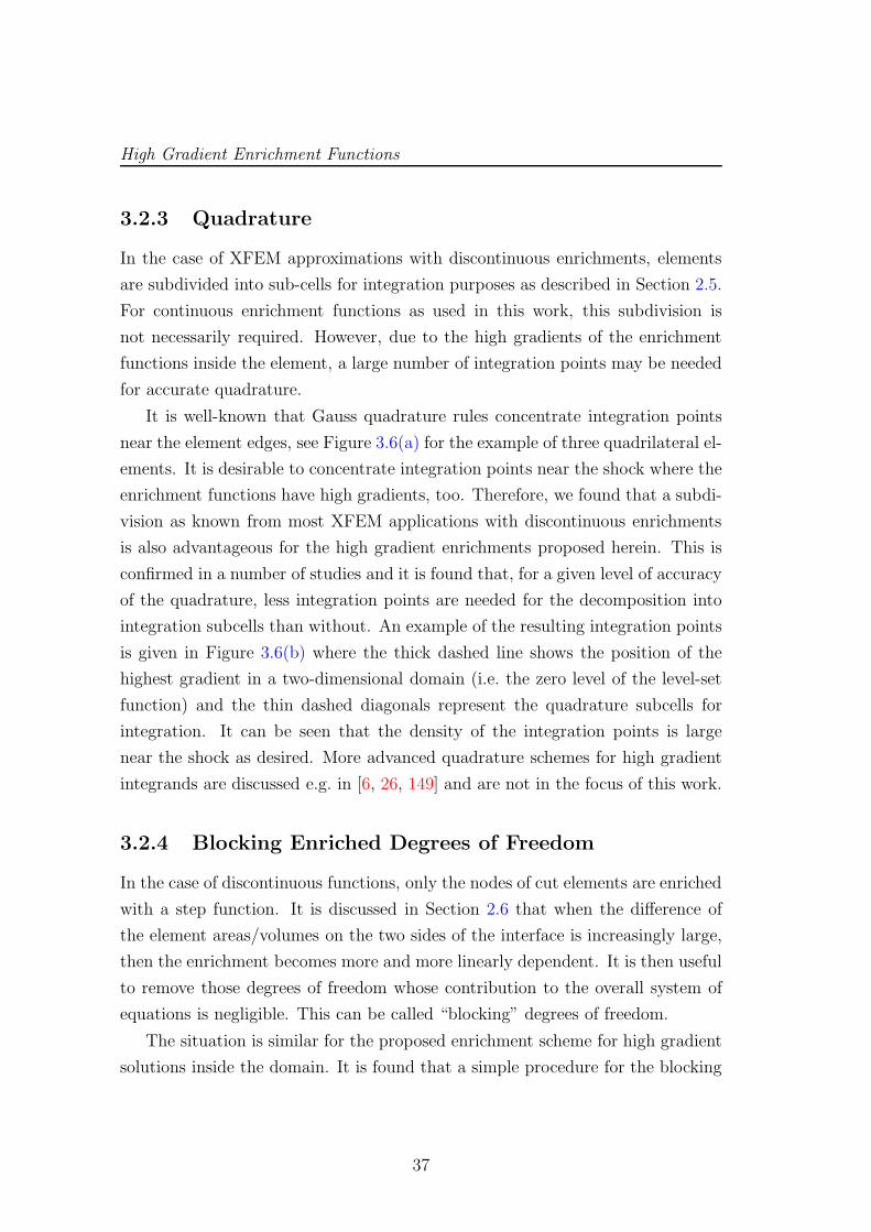
High Gradient Enrichment Functions
3.2.3 Quadrature
In the case of XFEM approximations with discontinuous enrichments, elements
are subdivided into sub-cells for integration purposes as described in Section 2.5.
For continuous enrichment functions as used in this work, this subdivision is
not necessarily required. However, due to the high gradients of the enrichment
functions inside the element, a large number of integration points may be needed
for accurate quadrature.
It is well-known that Gauss quadrature rules concentrate integration points
near the element edges, see Figure 3.6(a) for the example of three quadrilateral el-
ements. It is desirable to concentrate integration points near the shock where the
enrichment functions have high gradients, too. Therefore, we found that a subdi-
vision as known from most XFEM applications with discontinuous enrichments
is also advantageous for the high gradient enrichments proposed herein. This is
confirmed in a number of studies and it is found that, for a given level of accuracy
of the quadrature, less integration points are needed for the decomposition into
integration subcells than without. An example of the resulting integration points
is given in Figure 3.6(b) where the thick dashed line shows the position of the
highest gradient in a two-dimensional domain (i.e. the zero level of the level-set
function) and the thin dashed diagonals represent the quadrature subcells for
integration. It can be seen that the density of the integration points is large
near the shock as desired. More advanced quadrature schemes for high gradient
integrands are discussed e.g. in [6, 26, 149] and are not in the focus of this work.
3.2.4 Blocking Enriched Degrees of Freedom
In the case of discontinuous functions, only the nodes of cut elements are enriched
with a step function. It is discussed in Section 2.6 that when the difference of
the element areas/volumes on the two sides of the interface is increasingly large,
then the enrichment becomes more and more linearly dependent. It is then useful
to remove those degrees of freedom whose contribution to the overall system of
equations is negligible. This can be called “blocking” degrees of freedom.
The situation is similar for the proposed enrichment scheme for high gradient
solutions inside the domain. It is found that a simple procedure for the blocking
37
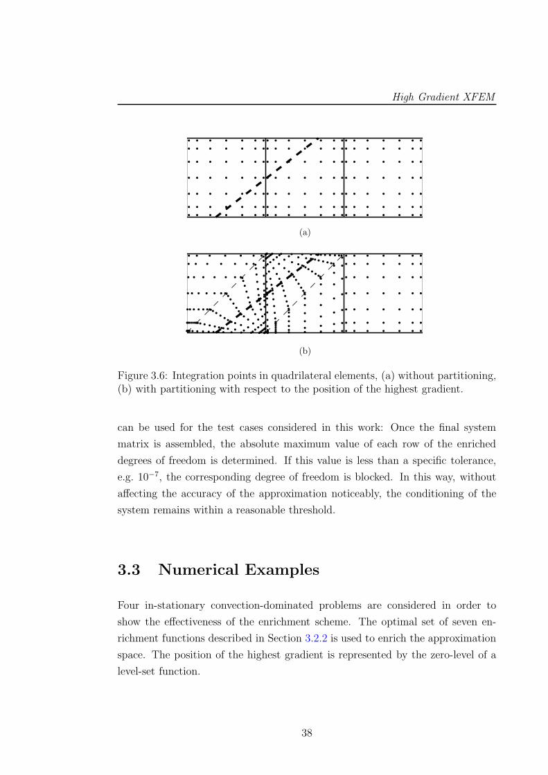
High Gradient XFEM
(a)
(b)
Figure 3.6: Integration points in quadrilateral elements, (a) without partitioning,(b) with partitioning with respect to the position of the highest gradient.
can be used for the test cases considered in this work: Once the final system
matrix is assembled, the absolute maximum value of each row of the enriched
degrees of freedom is determined. If this value is less than a specific tolerance,
e.g. 10−7, the corresponding degree of freedom is blocked. In this way, without
affecting the accuracy of the approximation noticeably, the conditioning of the
system remains within a reasonable threshold.
3.3 Numerical Examples
Four in-stationary convection-dominated problems are considered in order to
show the effectiveness of the enrichment scheme. The optimal set of seven en-
richment functions described in Section 3.2.2 is used to enrich the approximation
space. The position of the highest gradient is represented by the zero-level of a
level-set function.
38
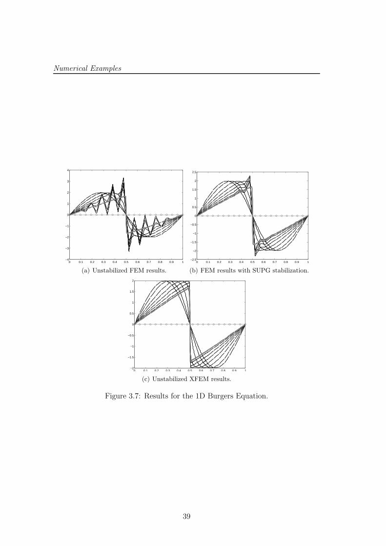
Numerical Examples
0 0.1 0.2 0.3 0.4 0.5 0.6 0.7 0.8 0.9 1−4
−3
−2
−1
0
1
2
3
4
(a) Unstabilized FEM results.
0 0.1 0.2 0.3 0.4 0.5 0.6 0.7 0.8 0.9 1−2.5
−2
−1.5
−1
−0.5
0
0.5
1
1.5
2
2.5
(b) FEM results with SUPG stabilization.
0 0.1 0.2 0.3 0.4 0.5 0.6 0.7 0.8 0.9 1−2
−1.5
−1
−0.5
0
0.5
1
1.5
2
(c) Unstabilized XFEM results.
Figure 3.7: Results for the 1D Burgers Equation.
39
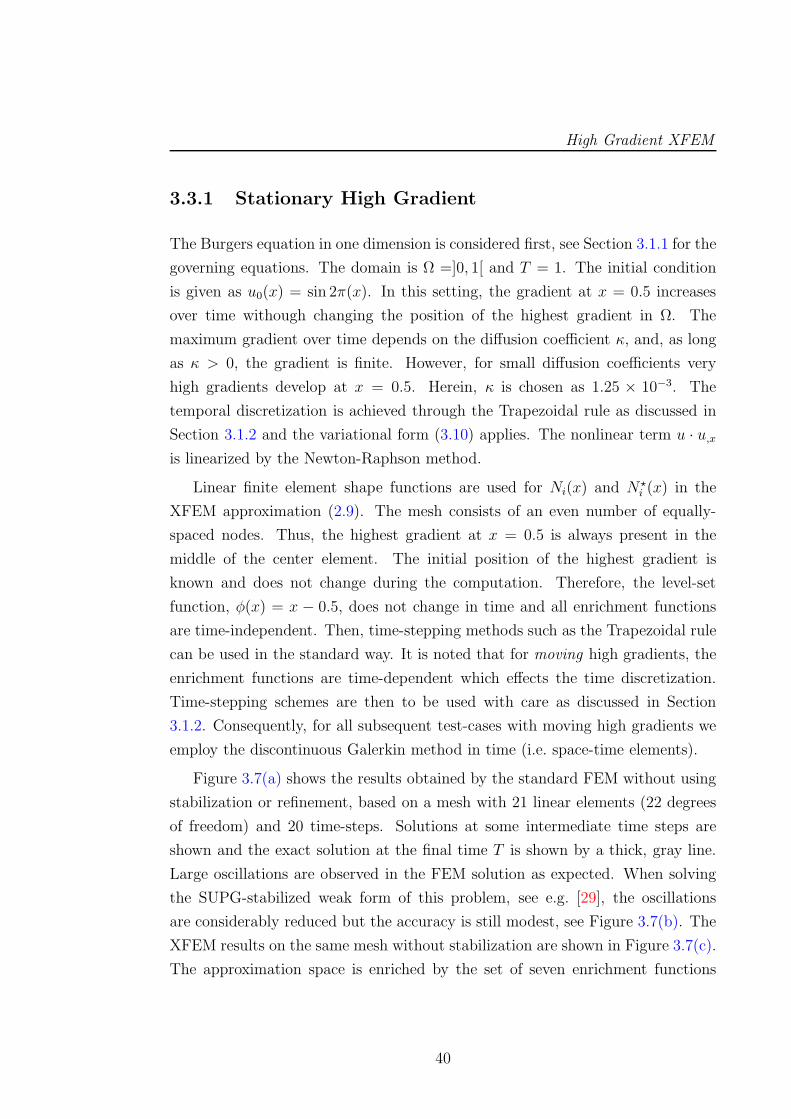
High Gradient XFEM
3.3.1 Stationary High Gradient
The Burgers equation in one dimension is considered first, see Section 3.1.1 for the
governing equations. The domain is Ω =]0, 1[ and T = 1. The initial condition
is given as u0(x) = sin 2π(x). In this setting, the gradient at x = 0.5 increases
over time withough changing the position of the highest gradient in Ω. The
maximum gradient over time depends on the diffusion coefficient κ, and, as long
as κ > 0, the gradient is finite. However, for small diffusion coefficients very
high gradients develop at x = 0.5. Herein, κ is chosen as 1.25 × 10⁻³. The
temporal discretization is achieved through the Trapezoidal rule as discussed in
Section 3.1.2 and the variational form (3.10) applies. The nonlinear term u · u,xis linearized by the Newton-Raphson method.
Linear finite element shape functions are used for Ni(x) and N⋆i (x) in the
XFEM approximation (2.9). The mesh consists of an even number of equally-
spaced nodes. Thus, the highest gradient at x = 0.5 is always present in the
middle of the center element. The initial position of the highest gradient is
known and does not change during the computation. Therefore, the level-set
function, φ(x) = x − 0.5, does not change in time and all enrichment functions
are time-independent. Then, time-stepping methods such as the Trapezoidal rule
can be used in the standard way. It is noted that for moving high gradients, the
enrichment functions are time-dependent which effects the time discretization.
Time-stepping schemes are then to be used with care as discussed in Section
3.1.2. Consequently, for all subsequent test-cases with moving high gradients we
employ the discontinuous Galerkin method in time (i.e. space-time elements).
Figure 3.7(a) shows the results obtained by the standard FEM without using
stabilization or refinement, based on a mesh with 21 linear elements (22 degrees
of freedom) and 20 time-steps. Solutions at some intermediate time steps are
shown and the exact solution at the final time T is shown by a thick, gray line.
Large oscillations are observed in the FEM solution as expected. When solving
the SUPG-stabilized weak form of this problem, see e.g. [29], the oscillations
are considerably reduced but the accuracy is still modest, see Figure 3.7(b). The
XFEM results on the same mesh without stabilization are shown in Figure 3.7(c).
The approximation space is enriched by the set of seven enrichment functions
40
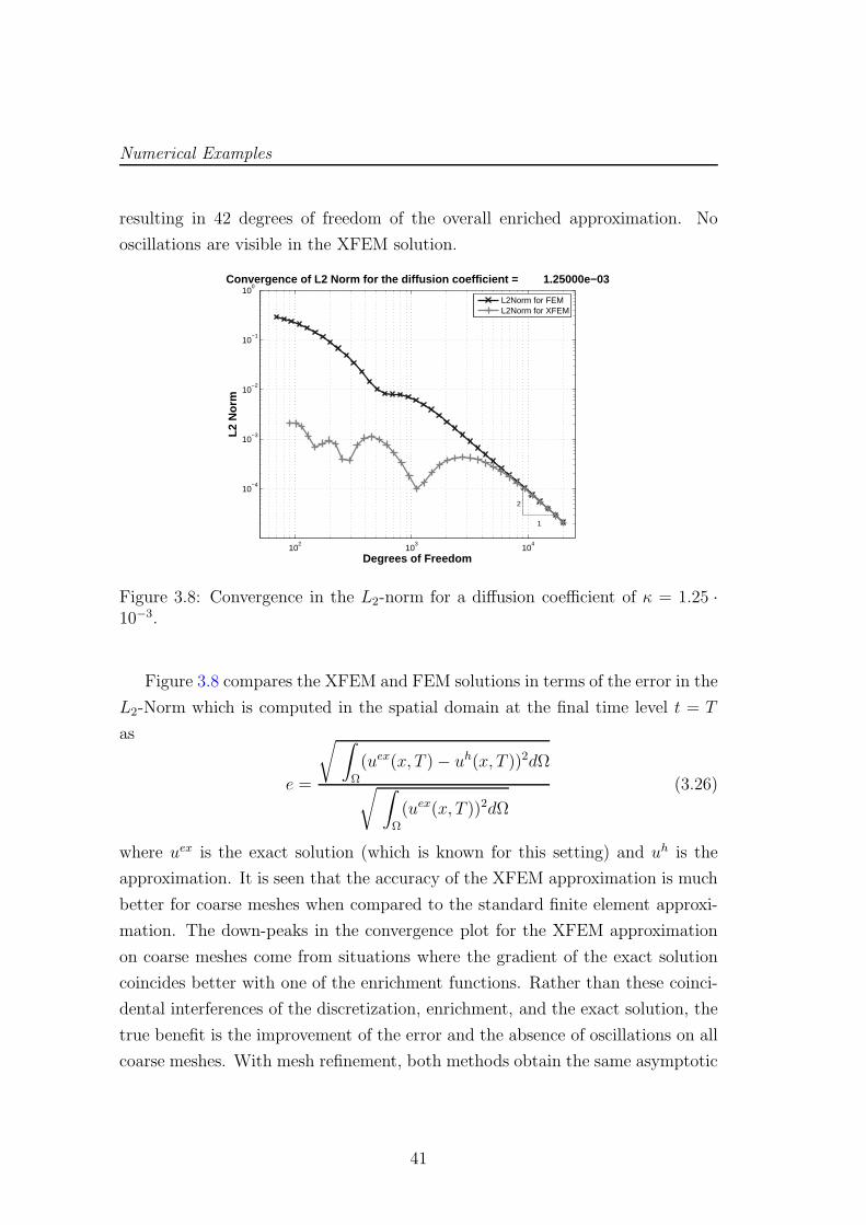
Numerical Examples
resulting in 42 degrees of freedom of the overall enriched approximation. No
oscillations are visible in the XFEM solution.
102
103
104
10−4
10−3
10−2
10−1
100
2
1
Degrees of Freedom
L2 N
orm
Convergence of L2 Norm for the diffusion coefficient = 1.25000e−03
L2Norm for FEML2Norm for XFEM
Figure 3.8: Convergence in the L2-norm for a diffusion coefficient of κ = 1.25 ·10−3.
Figure 3.8 compares the XFEM and FEM solutions in terms of the error in the
L2-Norm which is computed in the spatial domain at the final time level t = T
as
e =
√ ∫
Ω
(uex(x, T )− uh(x, T ))2dΩ
√ ∫
Ω
(uex(x, T ))2dΩ
(3.26)
where uex is the exact solution (which is known for this setting) and uh is the
approximation. It is seen that the accuracy of the XFEM approximation is much
better for coarse meshes when compared to the standard finite element approxi-
mation. The down-peaks in the convergence plot for the XFEM approximation
on coarse meshes come from situations where the gradient of the exact solution
coincides better with one of the enrichment functions. Rather than these coinci-
dental interferences of the discretization, enrichment, and the exact solution, the
true benefit is the improvement of the error and the absence of oscillations on all
coarse meshes. With mesh refinement, both methods obtain the same asymptotic
41
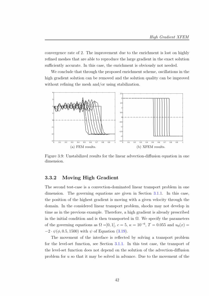
High Gradient XFEM
convergence rate of 2. The improvement due to the enrichment is lost on highly
refined meshes that are able to reproduce the large gradient in the exact solution
sufficiently accurate. In this case, the enrichment is obviously not needed.
We conclude that through the proposed enrichment scheme, oscillations in the
high gradient solution can be removed and the solution quality can be improved
without refining the mesh and/or using stabilization.
0 0.1 0.2 0.3 0.4 0.5 0.6 0.7 0.8 0.9 1−3
−2
−1
0
1
2
3
4
(a) FEM results.
0 0.1 0.2 0.3 0.4 0.5 0.6 0.7 0.8 0.9 1−2.5
−2
−1.5
−1
−0.5
0
0.5
1
1.5
2
2.5
(b) XFEM results.
Figure 3.9: Unstabilized results for the linear advection-diffusion equation in onedimension.
3.3.2 Moving High Gradient
The second test-case is a convection-dominated linear transport problem in one
dimension. The governing equations are given in Section 3.1.1. In this case,
the position of the highest gradient is moving with a given velocity through the
domain. In the considered linear transport problem, shocks may not develop in
time as in the previous example. Therefore, a high gradient is already prescribed
in the initial condition and is then transported in Ω. We specify the parameters
of the governing equations as Ω =]0, 1[, c = 5, κ = 10−6, T = 0.055 and u0(x) =
−2 · ψ(φ, 0.5, 1500) with ψ of Equation (3.19).
The movement of the interface is reflected by solving a transport problem
for the level-set function, see Section 3.1.1. In this test case, the transport of
the level-set function does not depend on the solution of the advection-diffusion
problem for u so that it may be solved in advance. Due to the movement of the
42
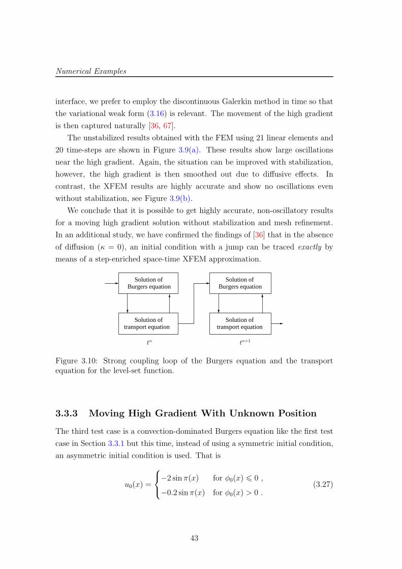
Numerical Examples
interface, we prefer to employ the discontinuous Galerkin method in time so that
the variational weak form (3.16) is relevant. The movement of the high gradient
is then captured naturally [36, 67].
The unstabilized results obtained with the FEM using 21 linear elements and
20 time-steps are shown in Figure 3.9(a). These results show large oscillations
near the high gradient. Again, the situation can be improved with stabilization,
however, the high gradient is then smoothed out due to diffusive effects. In
contrast, the XFEM results are highly accurate and show no oscillations even
without stabilization, see Figure 3.9(b).
We conclude that it is possible to get highly accurate, non-oscillatory results
for a moving high gradient solution without stabilization and mesh refinement.
In an additional study, we have confirmed the findings of [36] that in the absence
of diffusion (κ = 0), an initial condition with a jump can be traced exactly by
means of a step-enriched space-time XFEM approximation.
Solution oftransport equation
Burgers equationSolution of
Burgers equationSolution of
Solution oftransport equation
tn+1tn
Figure 3.10: Strong coupling loop of the Burgers equation and the transportequation for the level-set function.
3.3.3 Moving High Gradient With Unknown Position
The third test case is a convection-dominated Burgers equation like the first test
case in Section 3.3.1 but this time, instead of using a symmetric initial condition,
an asymmetric initial condition is used. That is
u0(x) =
−2 sin π(x) for φ0(x) 6 0 ,
−0.2 sin π(x) for φ0(x) > 0 .(3.27)
43
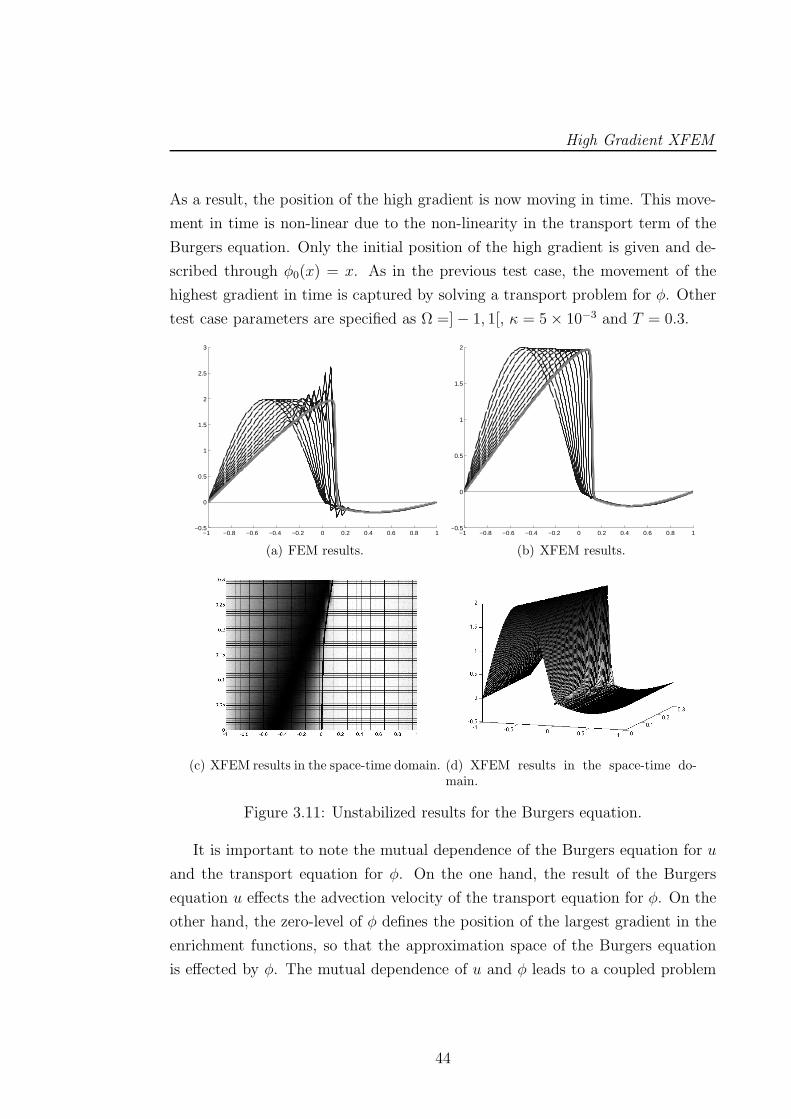
High Gradient XFEM
As a result, the position of the high gradient is now moving in time. This move-
ment in time is non-linear due to the non-linearity in the transport term of the
Burgers equation. Only the initial position of the high gradient is given and de-
scribed through φ0(x) = x. As in the previous test case, the movement of the
highest gradient in time is captured by solving a transport problem for φ. Other
test case parameters are specified as Ω =]− 1, 1[, κ = 5× 10⁻³ and T = 0.3.
−1 −0.8 −0.6 −0.4 −0.2 0 0.2 0.4 0.6 0.8 1−0.5
0
0.5
1
1.5
2
2.5
3
(a) FEM results.
−1 −0.8 −0.6 −0.4 −0.2 0 0.2 0.4 0.6 0.8 1−0.5
0
0.5
1
1.5
2
(b) XFEM results.
(c) XFEM results in the space-time domain. (d) XFEM results in the space-time do-main.
Figure 3.11: Unstabilized results for the Burgers equation.
It is important to note the mutual dependence of the Burgers equation for u
and the transport equation for φ. On the one hand, the result of the Burgers
equation u effects the advection velocity of the transport equation for φ. On the
other hand, the zero-level of φ defines the position of the largest gradient in the
enrichment functions, so that the approximation space of the Burgers equation
is effected by φ. The mutual dependence of u and φ leads to a coupled problem
44
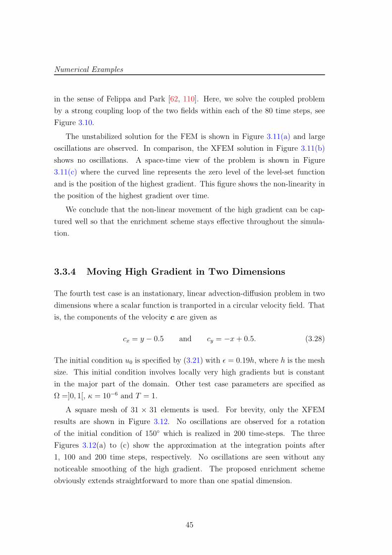
Numerical Examples
in the sense of Felippa and Park [62, 110]. Here, we solve the coupled problem
by a strong coupling loop of the two fields within each of the 80 time steps, see
Figure 3.10.
The unstabilized solution for the FEM is shown in Figure 3.11(a) and large
oscillations are observed. In comparison, the XFEM solution in Figure 3.11(b)
shows no oscillations. A space-time view of the problem is shown in Figure
3.11(c) where the curved line represents the zero level of the level-set function
and is the position of the highest gradient. This figure shows the non-linearity in
the position of the highest gradient over time.
We conclude that the non-linear movement of the high gradient can be cap-
tured well so that the enrichment scheme stays effective throughout the simula-
tion.
3.3.4 Moving High Gradient in Two Dimensions
The fourth test case is an instationary, linear advection-diffusion problem in two
dimensions where a scalar function is tranported in a circular velocity field. That
is, the components of the velocity c are given as
cx = y − 0.5 and cy = −x+ 0.5. (3.28)
The initial condition u0 is specified by (3.21) with ǫ = 0.19h, where h is the mesh
size. This initial condition involves locally very high gradients but is constant
in the major part of the domain. Other test case parameters are specified as
Ω =]0, 1[, κ = 10−6 and T = 1.
A square mesh of 31 × 31 elements is used. For brevity, only the XFEM
results are shown in Figure 3.12. No oscillations are observed for a rotation
of the initial condition of 150 which is realized in 200 time-steps. The three
Figures 3.12(a) to (c) show the approximation at the integration points after
1, 100 and 200 time steps, respectively. No oscillations are seen without any
noticeable smoothing of the high gradient. The proposed enrichment scheme
obviously extends straightforward to more than one spatial dimension.
45
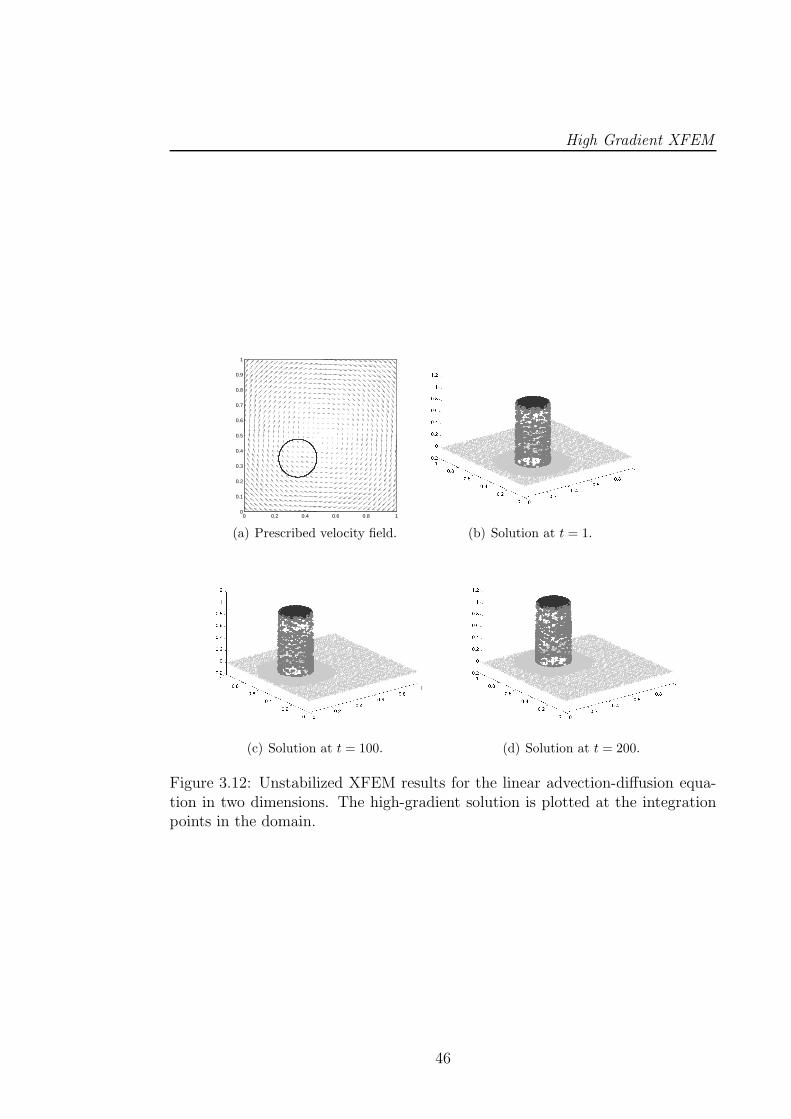
High Gradient XFEM
0 0.2 0.4 0.6 0.8 10
0.1
0.2
0.3
0.4
0.5
0.6
0.7
0.8
0.9
1
(a) Prescribed velocity field. (b) Solution at t = 1.
(c) Solution at t = 100. (d) Solution at t = 200.
Figure 3.12: Unstabilized XFEM results for the linear advection-diffusion equa-tion in two dimensions. The high-gradient solution is plotted at the integrationpoints in the domain.
46
Conclusions and Outlook
3.4 Conclusions and Outlook
A new variant of the XFEM called the HG-XFEM has been proposed. In the new
technique, high gradient fields inside the domain (shocks) are captured by a set of
enrichment functions used in the vicinity of the high gradients. The enrichment
functions are regularized step functions that depend on the distance from the
shock. The position of the highest gradient is described by the level-set function.
Moving shocks are considered for by solving an additional advection problem for
the level-set function.
After showing the success and potential of the HG-XFEM in the case of con-
vection dominated problems, the rest of this work will now focus on formulating
a model-independent XFEM-framework for simulating fracture problems. The
HG-XFEM will be used to capture the near-tip high gradient stress field for two
different fracture models in two and three dimensions.
47

High Gradient XFEM
48
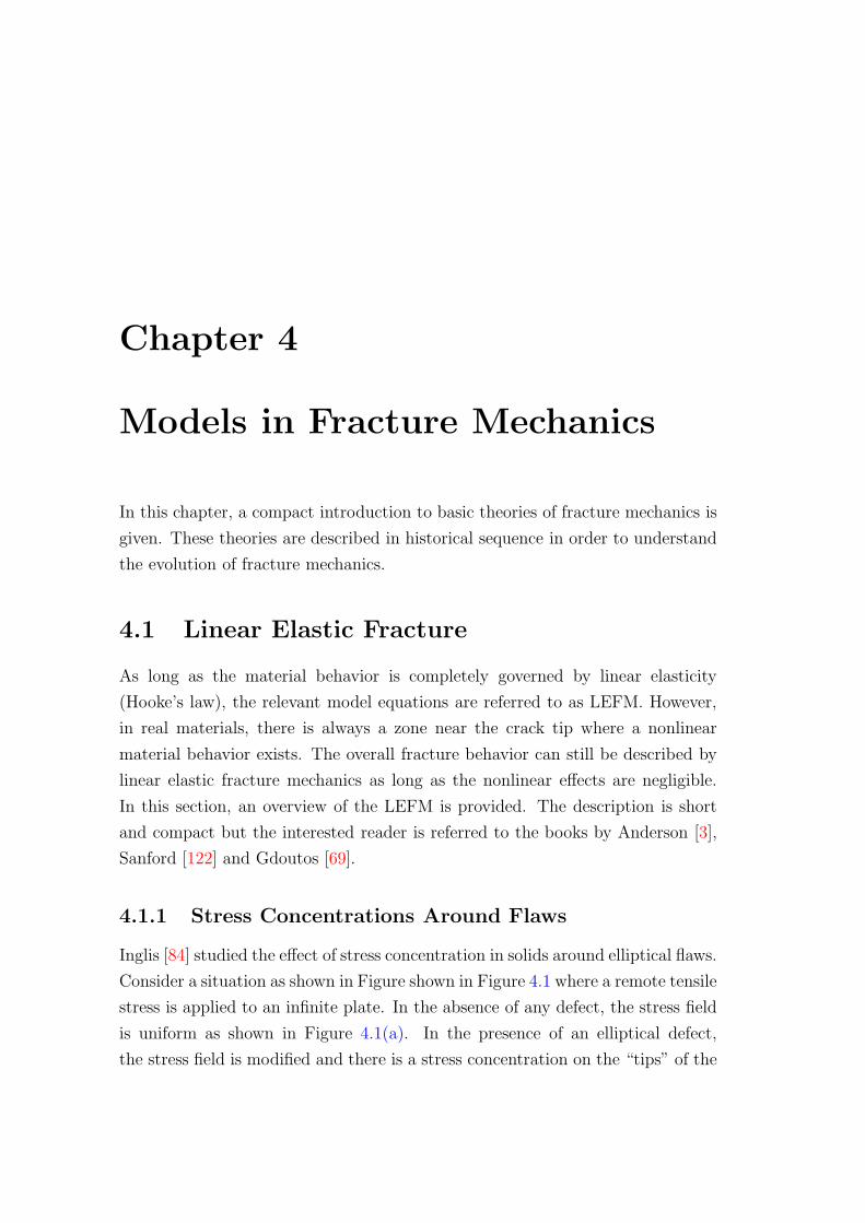
Chapter 4
Models in Fracture Mechanics
In this chapter, a compact introduction to basic theories of fracture mechanics is
given. These theories are described in historical sequence in order to understand
the evolution of fracture mechanics.
4.1 Linear Elastic Fracture
As long as the material behavior is completely governed by linear elasticity
(Hooke’s law), the relevant model equations are referred to as LEFM. However,
in real materials, there is always a zone near the crack tip where a nonlinear
material behavior exists. The overall fracture behavior can still be described by
linear elastic fracture mechanics as long as the nonlinear effects are negligible.
In this section, an overview of the LEFM is provided. The description is short
and compact but the interested reader is referred to the books by Anderson [3],
Sanford [122] and Gdoutos [69].
4.1.1 Stress Concentrations Around Flaws
Inglis [84] studied the effect of stress concentration in solids around elliptical flaws.
Consider a situation as shown in Figure shown in Figure 4.1 where a remote tensile
stress is applied to an infinite plate. In the absence of any defect, the stress field
is uniform as shown in Figure 4.1(a). In the presence of an elliptical defect,
the stress field is modified and there is a stress concentration on the “tips” of the
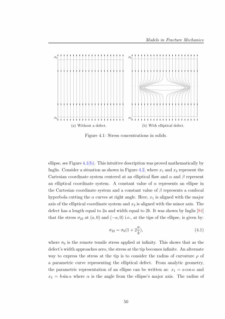
Models in Fracture Mechanics
σ0
σ0
(a) Without a defect.
σ0
σ0
(b) With elliptical defect.
Figure 4.1: Stress concentrations in solids.
ellipse, see Figure 4.1(b). This intuitive description was proved mathematically by
Inglis. Consider a situation as shown in Figure 4.2, where x1 and x2 represent the
Cartesian coordinate system centered at an elliptical flaw and α and β represent
an elliptical coordinate system. A constant value of α represents an ellipse in
the Cartesian coordinate system and a constant value of β represents a confocal
hyperbola cutting the α curves at right angle. Here, x1 is aligned with the major
axis of the elliptical coordinate system and x2 is aligned with the minor axis. The
defect has a length equal to 2a and width equal to 2b. It was shown by Inglis [84]
that the stress σ22 at (a, 0) and (−a, 0) i.e., at the tips of the ellipse, is given by:
σ22 = σ0(1 + 2a
b), (4.1)
where σ0 is the remote tensile stress applied at infinity. This shows that as the
defect’s width approaches zero, the stress at the tip becomes infinite. An alternate
way to express the stress at the tip is to consider the radius of curvature ρ of
a parametric curve representing the elliptical defect. From analytic geometry,
the parametric representation of an ellipse can be written as: x1 = a cosα and
x2 = b sinα where α is the angle from the ellipse’s major axis. The radius of
50
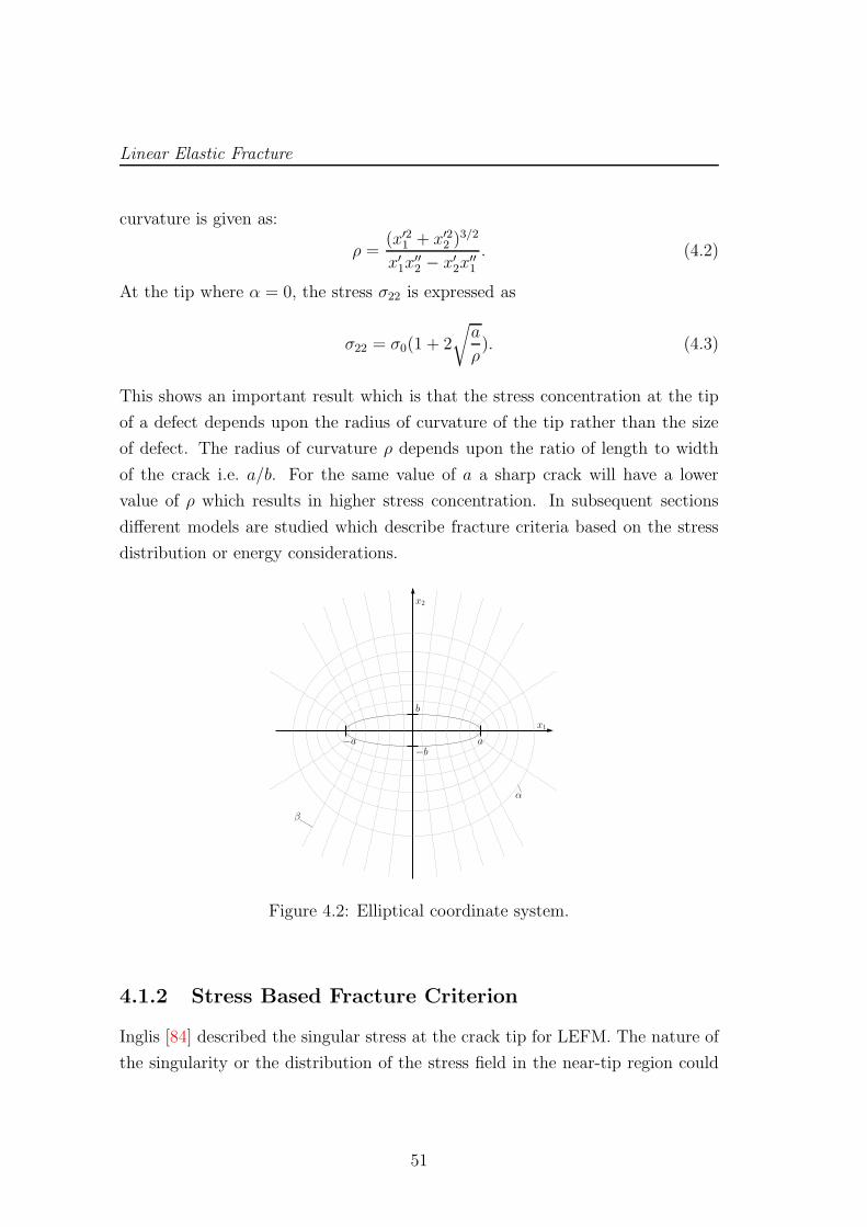
Linear Elastic Fracture
curvature is given as:
ρ =(x′21 + x′22 )
3/2
x′1x′′2 − x′2x
′′1
. (4.2)
At the tip where α = 0, the stress σ22 is expressed as
σ22 = σ0(1 + 2
√a
ρ). (4.3)
This shows an important result which is that the stress concentration at the tip
of a defect depends upon the radius of curvature of the tip rather than the size
of defect. The radius of curvature ρ depends upon the ratio of length to width
of the crack i.e. a/b. For the same value of a a sharp crack will have a lower
value of ρ which results in higher stress concentration. In subsequent sections
different models are studied which describe fracture criteria based on the stress
distribution or energy considerations.
b
x2
x1
β
α
a−a−b
Figure 4.2: Elliptical coordinate system.
4.1.2 Stress Based Fracture Criterion
Inglis [84] described the singular stress at the crack tip for LEFM. The nature of
the singularity or the distribution of the stress field in the near-tip region could
51
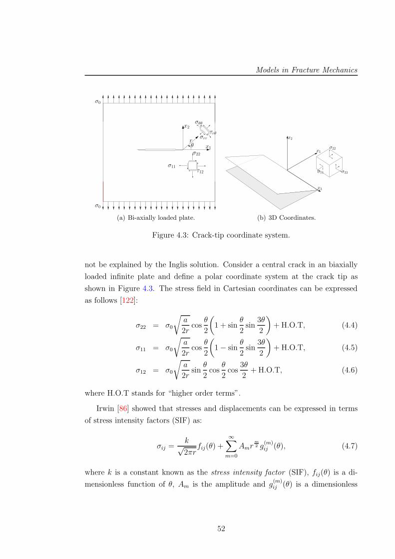
Models in Fracture Mechanics
σ0
τ12
τrθ
θr
x1
x2σθθ
σ22
σ11
σrr
σ0
(a) Bi-axially loaded plate.
σ33
x1
x2
x3
σ11
σ22
(b) 3D Coordinates.
Figure 4.3: Crack-tip coordinate system.
not be explained by the Inglis solution. Consider a central crack in an biaxially
loaded infinite plate and define a polar coordinate system at the crack tip as
shown in Figure 4.3. The stress field in Cartesian coordinates can be expressed
as follows [122]:
σ22 = σ0
√a
2rcos
θ
2
(
1 + sinθ
2sin
3θ
2
)
+H.O.T, (4.4)
σ11 = σ0
√a
2rcos
θ
2
(
1− sinθ
2sin
3θ
2
)
+H.O.T, (4.5)
σ12 = σ0
√a
2rsin
θ
2cos
θ
2cos
3θ
2+ H.O.T, (4.6)
where H.O.T stands for “higher order terms”.
Irwin [86] showed that stresses and displacements can be expressed in terms
of stress intensity factors (SIF) as:
σij =k√2πr
fij(θ) +
∞∑
m=0
Amrm2 g
(m)ij (θ), (4.7)
where k is a constant known as the stress intensity factor (SIF), fij(θ) is a di-
mensionless function of θ, Am is the amplitude and g(m)ij (θ) is a dimensionless
52
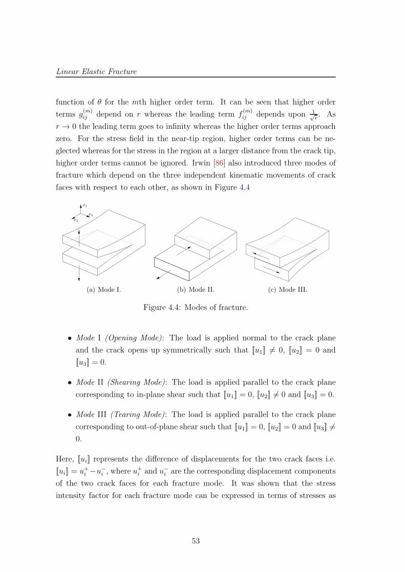
Linear Elastic Fracture
function of θ for the mth higher order term. It can be seen that higher order
terms g(m)ij depend on r whereas the leading term f
(m)ij depends upon 1√
r. As
r → 0 the leading term goes to infinity whereas the higher order terms approach
zero. For the stress field in the near-tip region, higher order terms can be ne-
glected whereas for the stress in the region at a larger distance from the crack tip,
higher order terms cannot be ignored. Irwin [86] also introduced three modes of
fracture which depend on the three independent kinematic movements of crack
faces with respect to each other, as shown in Figure 4.4
x2
x3
x1
(a) Mode I. (b) Mode II. (c) Mode III.
Figure 4.4: Modes of fracture.
• Mode I (Opening Mode): The load is applied normal to the crack plane
and the crack opens up symmetrically such that [[u1]] 6= 0, [[u2]] = 0 and
[[u3]] = 0.
• Mode II (Shearing Mode): The load is applied parallel to the crack plane
corresponding to in-plane shear such that [[u1]] = 0, [[u2]] 6= 0 and [[u3]] = 0.
• Mode III (Tearing Mode): The load is applied parallel to the crack plane
corresponding to out-of-plane shear such that [[u1]] = 0, [[u2]] = 0 and [[u3]] 6=0.
Here, [[ui]] represents the difference of displacements for the two crack faces i.e.
[[ui]] = u+i −u−i , where u+i and u−i are the corresponding displacement components
of the two crack faces for each fracture mode. It was shown that the stress
intensity factor for each fracture mode can be expressed in terms of stresses as
53
Models in Fracture Mechanics
follows:
KI
KII
KIII
= limr→0,θ=0
√2πr
σ22
σ12
σ23
, (4.8)
where KI, KII and KIII are the stress intensity factors associated with each frac-
ture mode respectively. Stress at any point in the near-tip field can be obtained
exactly by a linear combination of stresses due to each mode of fracture
σij = σIij + σII
ij + σIIIij . (4.9)
From Eq. (4.7), the stress field due to each fracture mode can be given as:
σIij =
KI√2πr
f Iij(θ), σII
ij =KII√2πr
f IIij (θ) and σIII
ij =KIII√2πr
f IIIij (θ). (4.10)
Stress intensity factors give the intensity of the singular stress field due to re-
spective fracture mode whereas other factors in Eq. (4.10), i.e. r and fij , give the
distribution of the stress field. An interesting overview of experimental as well as
numerical methods to compute stress intensity factors is given by Sanford [122].
For the propagation of a given crack, there exists a critical value of the SIF called
the critical stress intensity factor Kc. It is a measure of the fracture toughness of
a material. It is a material property and is independent of the specimen geome-
try. The value of Kc for a given material is determined experimentally [122]. As
the majority of materials fail in tension rather than in shear, the critical stress
intensity factor usually refers to the mode I failure, i.e., at failure
KI = KIc . (4.11)
Stress and displacement fields for the three modes of fracture in Cartesian coor-
dinates are given as follows:
54
Linear Elastic Fracture
Pure mode I loading:
σxx =KI√2πr
cosθ
2
(
1− sinθ
2sin
3θ
2
)
, (4.12a)
σyy =KI√2πr
cosθ
2
(
1 + sinθ
2sin
3θ
2
)
, (4.12b)
σzz = ν(σxx + σyy), (4.12c)
τxy =KI√2πr
sinθ
2cos
θ
2cos
3θ
2, (4.12d)
τxz = τyz = 0 (4.12e)
u =KI
2µ
√r
2πcos
θ
2
(
κ− 1 + 2 sin2 θ
2
)
, (4.12f)
v =KI
2µ
√r
2πsin
θ
2
(
κ+ 1− 2 cos2θ
2
)
, (4.12g)
w = 0. (4.12h)
Pure mode II loading:
σxx = − KII√2πr
sinθ
2
(
2 + cosθ
2cos
3θ
2
)
, (4.13a)
σyy =KII√2πr
sinθ
2cos
θ
2cos
3θ
2, (4.13b)
σzz = ν(σxx + σyy), (4.13c)
τxy =KII√2πr
cosθ
2
(
1− sinθ
2sin
3θ
2
)
, (4.13d)
τxz = τyz = 0, (4.13e)
u =KII
2µ
√r
2πsin
θ
2
(
κ + 1 + 2 cos2θ
2
)
, (4.13f)
v = −KII
2µ
√r
2πcos
θ
2
(
κ− 1− 2 sin2 θ
2
)
, (4.13g)
w = 0. (4.13h)
55
Models in Fracture Mechanics
Pure mode III loading:
σxx = σyy = σzz = τxy = 0, (4.14a)
τxz = − KIII√2πr
sinθ
2, (4.14b)
τyz =KIII√2πr
cosθ
2, (4.14c)
u = v = 0, (4.14d)
w =KIII
µ
√
2r
πsin
θ
2. (4.14e)
Expressing these stresses in polar coordinates gives the following expressions for
the pure mode I and II loading.
Pure mode I loading:
σrr =KI√2πr
cosθ
2
(
1 + sin2 θ
2
)
, (4.15a)
σθθ =KI√2πr
cosθ
2
(
1− sin2 θ
2
)
, (4.15b)
τrθ =KI√2πr
sinθ
2cos2
θ
2. (4.15c)
Pure mode II loading:
σrr =KII√2πr
(
− 5
4sin
θ
2+
3
4sin
3θ
2
)
, (4.16a)
σθθ =KII√2πr
(
− 3
4sin
θ
2− 3
4sin
3θ
2
)
, (4.16b)
τrθ =KII√2πr
(1
4cos
θ
2+
3
4cos
3θ
2
)
. (4.16c)
4.1.3 Energy Based Fracture Criterion
Griffith [75] motivated an energy based description of fracture. He realized the
possibility of a thermodynamic criterion for crack propagation. The first law of
thermodynamics as given by Clausius [41] states that:
56
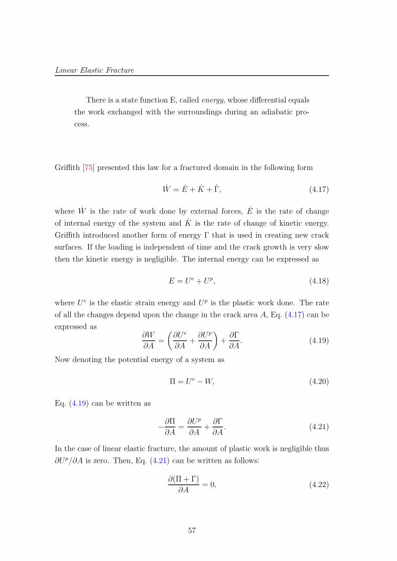
Linear Elastic Fracture
There is a state function E, called energy, whose differential equals
the work exchanged with the surroundings during an adiabatic pro-
cess.
Griffith [75] presented this law for a fractured domain in the following form
W = E + K + Γ, (4.17)
where W is the rate of work done by external forces, E is the rate of change
of internal energy of the system and K is the rate of change of kinetic energy.
Griffith introduced another form of energy Γ that is used in creating new crack
surfaces. If the loading is independent of time and the crack growth is very slow
then the kinetic energy is negligible. The internal energy can be expressed as
E = Ue + Up, (4.18)
where Ue is the elastic strain energy and Up is the plastic work done. The rate
of all the changes depend upon the change in the crack area A, Eq. (4.17) can be
expressed as∂W
∂A=
(∂Ue
∂A+∂Up
∂A
)
+∂Γ
∂A. (4.19)
Now denoting the potential energy of a system as
Π = Ue −W, (4.20)
Eq. (4.19) can be written as
−∂Π∂A
=∂Up
∂A+∂Γ
∂A. (4.21)
In the case of linear elastic fracture, the amount of plastic work is negligible thus
∂Up/∂A is zero. Then, Eq. (4.21) can be written as follows:
∂(Π + Γ)
∂A= 0, (4.22)
57
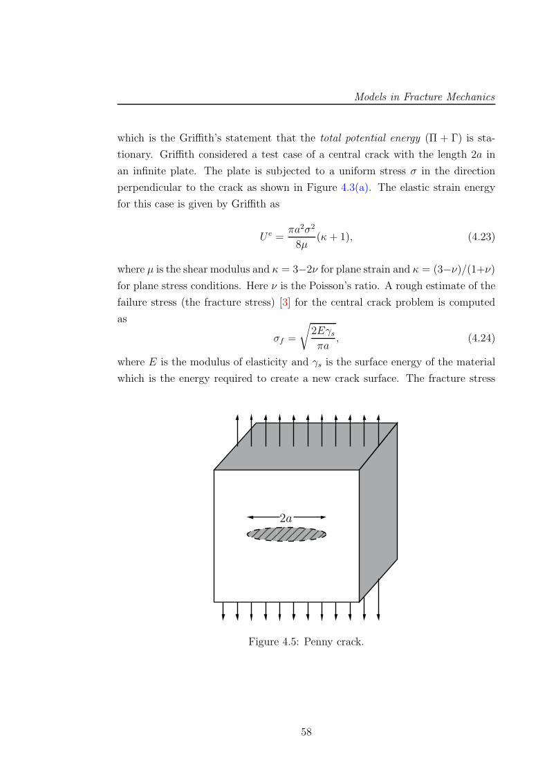
Models in Fracture Mechanics
which is the Griffith’s statement that the total potential energy (Π + Γ) is sta-
tionary. Griffith considered a test case of a central crack with the length 2a in
an infinite plate. The plate is subjected to a uniform stress σ in the direction
perpendicular to the crack as shown in Figure 4.3(a). The elastic strain energy
for this case is given by Griffith as
Ue =πa2σ2
8µ(κ+ 1), (4.23)
where µ is the shear modulus and κ = 3−2ν for plane strain and κ = (3−ν)/(1+ν)for plane stress conditions. Here ν is the Poisson’s ratio. A rough estimate of the
failure stress (the fracture stress) [3] for the central crack problem is computed
as
σf =
√
2Eγsπa
, (4.24)
where E is the modulus of elasticity and γs is the surface energy of the material
which is the energy required to create a new crack surface. The fracture stress
2a
Figure 4.5: Penny crack.
58
Linear Elastic Fracture
for a penny crack as shown in Figure 4.5 is computed as
σf =
√
πEγs2(1− ν2)a
. (4.25)
Equation (4.24) and (4.25) are only valid for brittle materials like glass. For
quasi brittle materials, the fracture stress is overestimated. In order to consider
for that, Orowan [106] and Irwin [85] added another factor γp that represents
the plastic work done per unit area of surface created. This parameter is several
orders of magnitude larger than the γs. Thus Eq. (4.24) can be expressed as
σf =
√
2E(γs + γp)
πa. (4.26)
In a more general sense, a parameter γw is used that consists of elastic, plastic,
viscoelastic or viscoplastic work done per unit area of surface created,
σf =
√
2Eγwπa
. (4.27)
It should be noted that Eq. (4.27) can only be used in the case where the global
behavior of the material is linear elastic and all the nonlinear effects are confined
in a small area near the crack tip.
Irwin [86] described the approach of the energy release rate as a criterion for
crack extension. Rearranging Eq. (4.22) gives
− ∂(Π)
∂A=
∂(Γ)
∂A, (4.28)
−∂(Ue −W )
∂A︸ ︷︷ ︸
G
=∂(Γ)
∂A︸ ︷︷ ︸
Gc
, (4.29)
where the left hand side is called the energy release rate and is denoted by G after
Griffith. The right hand side gives the critical value of Gc which must be overcome
for a crack to propagate similar to the critical stress intensity factor given in
Eq. (4.11). Steinmann [126] proved the relation between the stress intensity
59
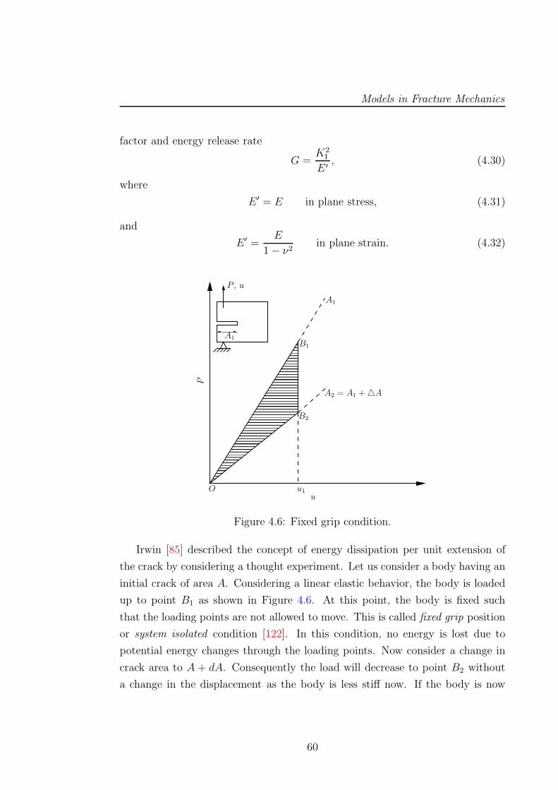
Models in Fracture Mechanics
factor and energy release rate
G =K2
I
E ′ , (4.30)
where
E ′ = E in plane stress, (4.31)
and
E ′ =E
1− ν2in plane strain. (4.32)
u1
P , u
A1
O
B1
B2
A1
A2 = A1 +A
u
P
Figure 4.6: Fixed grip condition.
Irwin [85] described the concept of energy dissipation per unit extension of
the crack by considering a thought experiment. Let us consider a body having an
initial crack of area A. Considering a linear elastic behavior, the body is loaded
up to point B1 as shown in Figure 4.6. At this point, the body is fixed such
that the loading points are not allowed to move. This is called fixed grip position
or system isolated condition [122]. In this condition, no energy is lost due to
potential energy changes through the loading points. Now consider a change in
crack area to A + dA. Consequently the load will decrease to point B2 without
a change in the displacement as the body is less stiff now. If the body is now
60
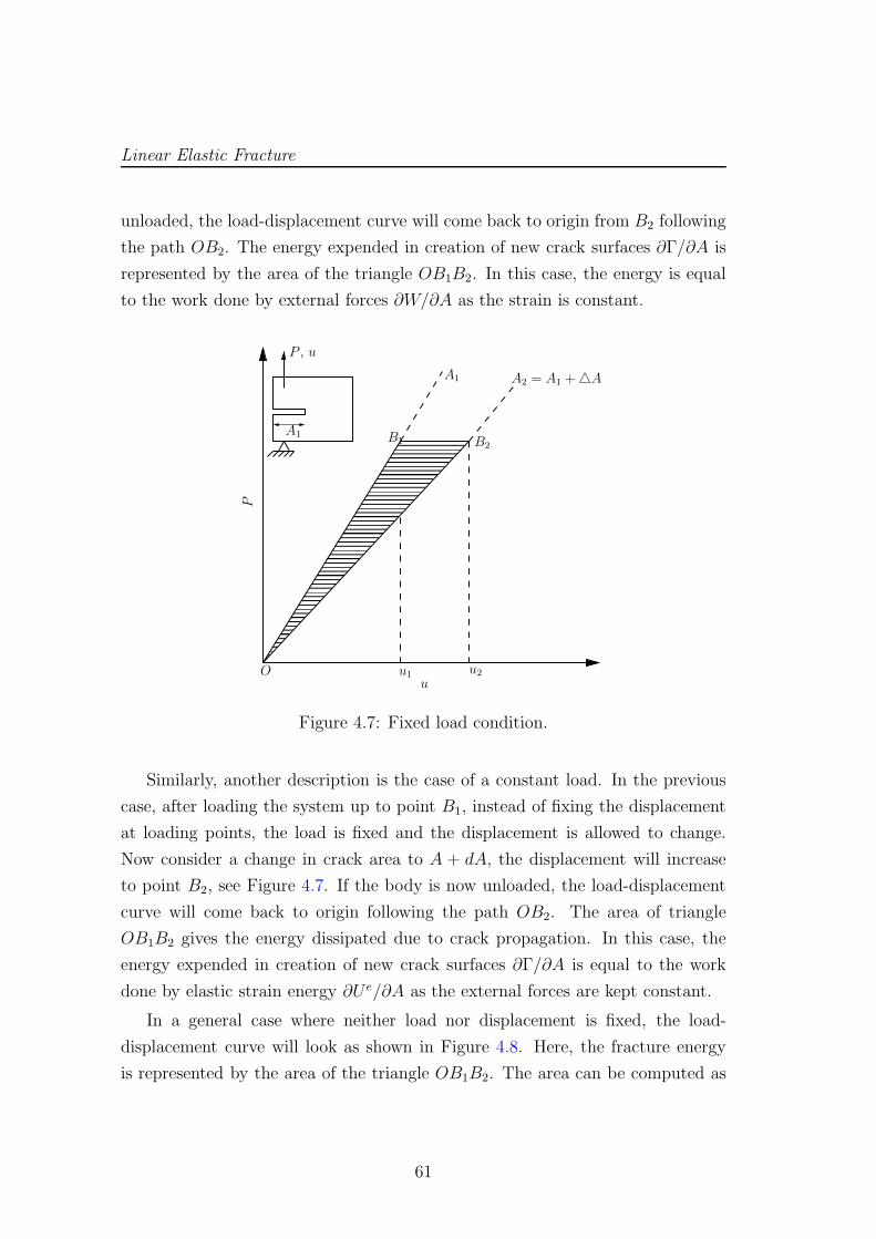
Linear Elastic Fracture
unloaded, the load-displacement curve will come back to origin from B2 following
the path OB2. The energy expended in creation of new crack surfaces ∂Γ/∂A is
represented by the area of the triangle OB1B2. In this case, the energy is equal
to the work done by external forces ∂W/∂A as the strain is constant.
B2
P , u
A1
O
A1
u
P
u1
B1
A2 = A1 +A
u2
Figure 4.7: Fixed load condition.
Similarly, another description is the case of a constant load. In the previous
case, after loading the system up to point B1, instead of fixing the displacement
at loading points, the load is fixed and the displacement is allowed to change.
Now consider a change in crack area to A + dA, the displacement will increase
to point B2, see Figure 4.7. If the body is now unloaded, the load-displacement
curve will come back to origin following the path OB2. The area of triangle
OB1B2 gives the energy dissipated due to crack propagation. In this case, the
energy expended in creation of new crack surfaces ∂Γ/∂A is equal to the work
done by elastic strain energy ∂Ue/∂A as the external forces are kept constant.
In a general case where neither load nor displacement is fixed, the load-
displacement curve will look as shown in Figure 4.8. Here, the fracture energy
is represented by the area of the triangle OB1B2. The area can be computed as
61
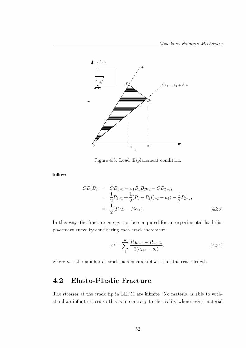
Models in Fracture Mechanics
A2 = A1 +A
P , u
A1
O
A1
u
P
u1
B1
u2
B2
Figure 4.8: Load displacement condition.
follows
OB1B2 = OB1u1 + u1B1B2u2 −OB2u2,
=1
2P1u1 +
1
2(P1 + P2)(u2 − u1)−
1
2P2u2,
=1
2(P1u2 − P2u1). (4.33)
In this way, the fracture energy can be computed for an experimental load dis-
placement curve by considering each crack increment
G =n∑
i
Piui+1 − Pi+1ui2(ai+1 − ai)
, (4.34)
where n is the number of crack increments and a is half the crack length.
4.2 Elasto-Plastic Fracture
The stresses at the crack tip in LEFM are infinite. No material is able to with-
stand an infinite stress so this is in contrary to the reality where every material
62
Elasto-Plastic Fracture
has finite strength. This discrepancy is due to to the assumption of a sharp crack
tip. In reality, an ideally sharp crack tip does not exist. Wells [143] realized that
crack faces move apart due to plastic deformation before the fracture occurs. This
blunts the crack tip thus limiting the stresses at the crack tip. The amount of
blunting depends upon the ductility of the material and the size of a specimen.
In very brittle materials like glass this blunting can be ignored. Sometimes, the
ductile behavior cannot be ignored in a laboratory size specimen whereas in large
structures like dams this behavior can be ignored. In case the plastic effects are
negligible, a crack can be analyzed by the LEFM. If the plastic effects cannot be
ignored, the size of the plastic zone is estimated and plasticity models are applied
to the plastic zone. The bulk of the material can be analyzed by the LEFM.
4.2.1 Size of the Plastic Zone
Principal stresses in the near-tip region are given as
σ1,2 =σxx + σyy
2±
√(σxx − σyy
2
)2
+ τ 2xy. (4.35)
Inserting the values of σxx, σyy and τxy from Eq. (4.12) into Eq. (4.35) and solving
for principle stresses gives the following principle stresses for mode I fracture
σ1 =KI√2πr
cosθ
2
(
1 + sinθ
2
)
, (4.36a)
σ2 =KI√2πr
cosθ
2
(
1− sinθ
2
)
, (4.36b)
σ3 = ν(σ1 + σ2) for plane strain, (4.36c)
σ3 = 0 for plane stress. (4.36d)
The approximate size of the plastic zone can be found by introducing the principle
stress into any yield criterion such as the von-Mises yield criterion
σyld =
√
(σ1 − σ2)2 + (σ2 − σ3)2 + (σ3 − σ1)2
2. (4.37)
63
Models in Fracture Mechanics
Inserting Eq. (4.36) in Eq. (4.37) and solving for the size of the plastic zone rp
gives
rp =1
4π
(KI
σyld
)2 [
1 +3
2sin2 θ + cos θ
]
for plane stress, (4.38)
rp =1
4π
(KI
σyld
)2 [3
2sin2 θ + (1− 2ν)2(1 + cos θ)
]
for plane strain.(4.39)
For the plastic zone along the crack axis i.e., at θ = 0
rp =1
2π
(KI
σyld
)2
for plane stress, (4.40)
rp =1
4π
(KI
σyld
)2
for plane strain. (4.41)
Irwin [86] estimated the size of a plastic zone as cp = 2rp i.e., due to plastic effects
the crack behaves as if it is larger than its size. This extra length is computed by
some stress redistribution along the crack axis as
cp =1
nπ
(K
σyld
)2
, (4.42)
where n = 1 for plane stress and n = 3 for plane strain.
4.2.2 Crack Propagation Criteria
In elasto-plastic fracture mechanics two criteria are used as fracture criteria. The
first is the crack tip opening displacement (CTOD) which is based on a local
criterion and the second is the path independent J-integral which is based on a
global criterion.
4.2.2.1 Crack Tip Opening Displacement (CTOD)
Wells [143] and Cottrell [44] introduced the concept of crack tip opening displace-
ment (CTOD) as a criterion for elasto-plastic fracture. As stresses near the crack
tip reach a critical value, the crack faces move apart from each other. The frac-
ture occurs due to void formation and coalescence. In concrete, micro-cracking
64
Elasto-Plastic Fracture
takes place instead of void formation. The CTOD, denoted by δ, is described
as the separation of crack faces which gives a measure of plastic deformation. A
crack propagates only when the value of δ reaches a critical value δc. This critical
value, which is a material constant, is independent of the specimen configuration
and crack length [69]. From Eq. (4.12) the normal displacement for a horizontal
crack is given as
v =KI
2µ
√r
2πsin
θ
2
(
κ+ 1− 2 cos2θ
2
)
. (4.43)
Using θ = ±π gives the displacement of upper and lower crack faces and their
sum gives the value of the CTOD as
2v = δ =κ+ 1
µKI
√r
2π. (4.44)
Using the estimate of the size of plastic zone from Irwin for the case of plane
stress from Eq. (4.42) and using κ = 3−ν1+ν
, the critical value of the CTOD is given
as
δc =4
π
K2I
Eσyld. (4.45)
Using Dugdale’s model, the CTOD is given as
δc =K2
I
Eσyld
[
1 +π2
24
σ2
σ2yld
+ · · ·]
. (4.46)
For small values ofσ2
σ2yld
, Eq. (4.46) reduces to
δc =K2
I
Eσyld. (4.47)
4.2.2.2 J-Intergral
The path-independent J-Integral [60] was introduced as a fracture criterion by
Rice [120]. Its use as a criterion in fracture mechanics is motivated by considering
an elasto-plastic material as nonlinear elastic. This behavior can be explained
with Figure 4.9 which shows the uniaxial stress-strain relation for a nonlinear
65
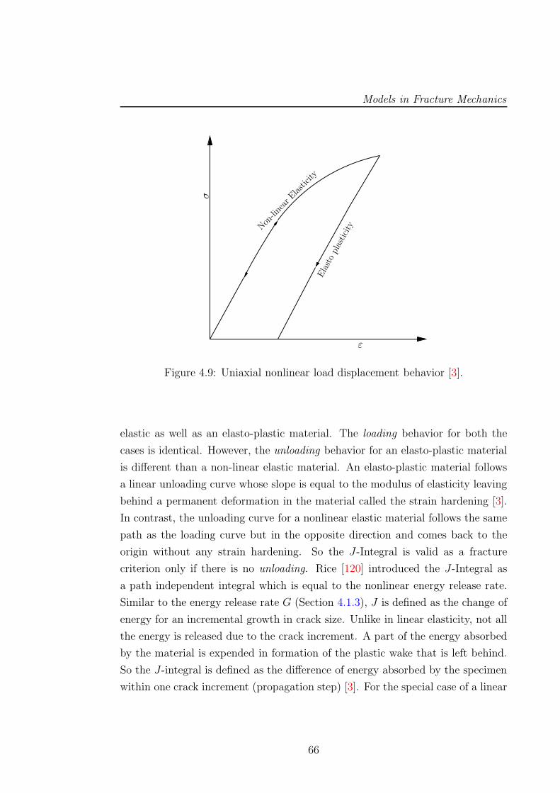
Models in Fracture Mechanics
ε
Non-linearElasticity
Elastoplasticity
σ
Figure 4.9: Uniaxial nonlinear load displacement behavior [3].
elastic as well as an elasto-plastic material. The loading behavior for both the
cases is identical. However, the unloading behavior for an elasto-plastic material
is different than a non-linear elastic material. An elasto-plastic material follows
a linear unloading curve whose slope is equal to the modulus of elasticity leaving
behind a permanent deformation in the material called the strain hardening [3].
In contrast, the unloading curve for a nonlinear elastic material follows the same
path as the loading curve but in the opposite direction and comes back to the
origin without any strain hardening. So the J-Integral is valid as a fracture
criterion only if there is no unloading. Rice [120] introduced the J-Integral as
a path independent integral which is equal to the nonlinear energy release rate.
Similar to the energy release rate G (Section 4.1.3), J is defined as the change of
energy for an incremental growth in crack size. Unlike in linear elasticity, not all
the energy is released due to the crack increment. A part of the energy absorbed
by the material is expended in formation of the plastic wake that is left behind.
So the J-integral is defined as the difference of energy absorbed by the specimen
within one crack increment (propagation step) [3]. For the special case of a linear
66
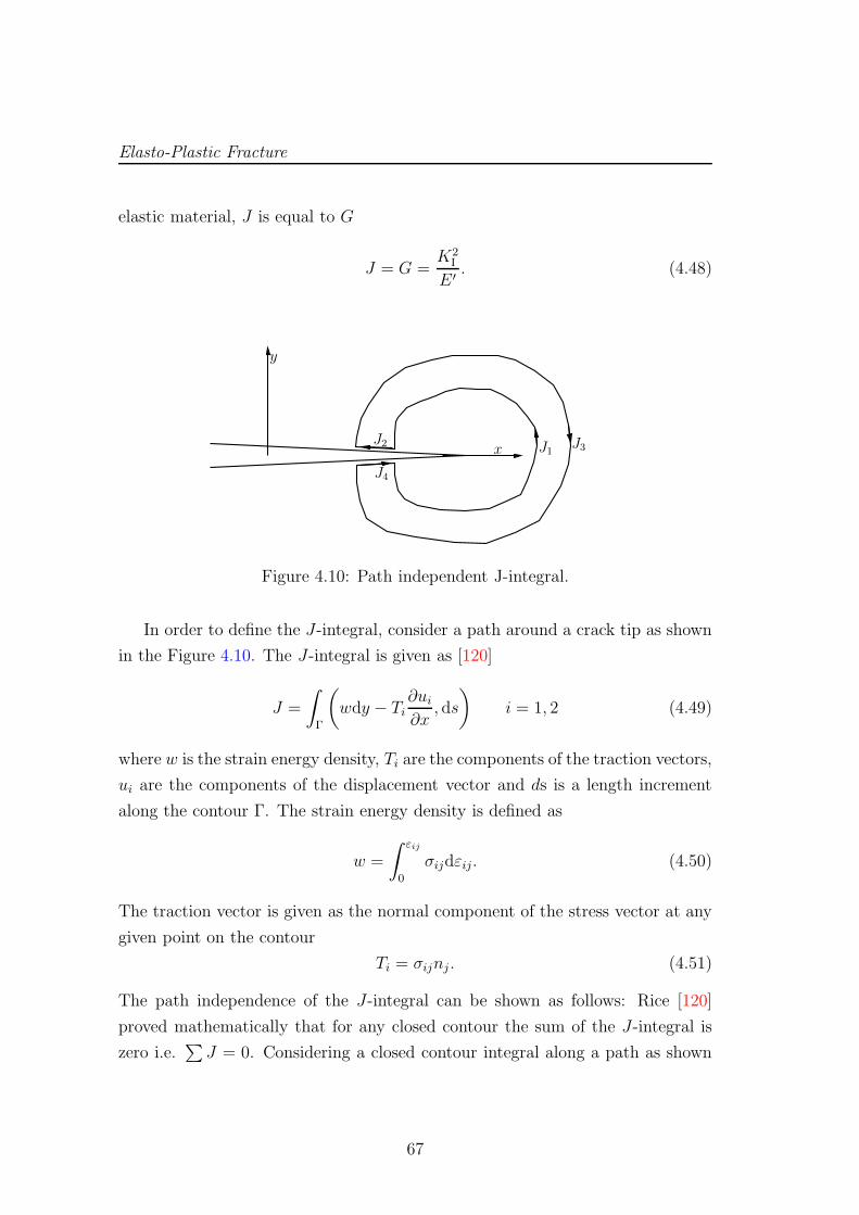
Elasto-Plastic Fracture
elastic material, J is equal to G
J = G =K2
I
E ′ . (4.48)
J4
x
y
J1 J3J2
Figure 4.10: Path independent J-integral.
In order to define the J-integral, consider a path around a crack tip as shown
in the Figure 4.10. The J-integral is given as [120]
J =
∫
Γ
(
wdy − Ti∂ui∂x
, ds
)
i = 1, 2 (4.49)
where w is the strain energy density, Ti are the components of the traction vectors,
ui are the components of the displacement vector and ds is a length increment
along the contour Γ. The strain energy density is defined as
w =
∫ εij
0
σijdεij. (4.50)
The traction vector is given as the normal component of the stress vector at any
given point on the contour
Ti = σijnj . (4.51)
The path independence of the J-integral can be shown as follows: Rice [120]
proved mathematically that for any closed contour the sum of the J-integral is
zero i.e.∑J = 0. Considering a closed contour integral along a path as shown
67
Models in Fracture Mechanics
in Figure 4.10∑
J = J1 + J2 + J3 + J4 = 0. (4.52)
As the crack faces Γ2 and Γ4 are stress free, J2 = J4 = 0, and it is shown in [120]
that J1 = −J3 which proves the path independence of the J-integral.
Hutchinson [82], Rice & Rosengren [121] described the J-Integral as a stress
intensity parameter. They showed that the stress and the strain fields in the near
tip region can be characterized by the J-integral
σ = k1
(J
r
) 1n+1
, (4.53a)
ε = k2
(J
r
) nn+1
, (4.53b)
where k1 and k2 are proportionality constants and n is the strain hardening
exponent. Details about how to compute these constants can be found in Rice &
Rosengren [121].
4.3 Fracture Process Zone Modeling
The nonlinear material behavior near a crack tip can be modeled as a fracture
process zone (FPZ). A fracture process zone can be defined as the zone where
void formation and coalescence takes place in the case of ductile materials or
where micro cracking occurs in the case of cementitious materials or rocks. In
FPZ modeling, plastic effects along the crack path are modeled considering the
fracture process zone. This circumvents some of the disadvantages related to
LEFM and EPFM. As described by Cotterell [43], the disadvantages of the LEFM
are:
• The LEFM can only be used if there is an initial crack, crack-like defect or
notch. In contrast, FPZ modeling allows for a crack initiation criteria.
• The LEFM is valid only when the FPZ is negligible in size as compared to
the overall dimensions of the specimen.
68
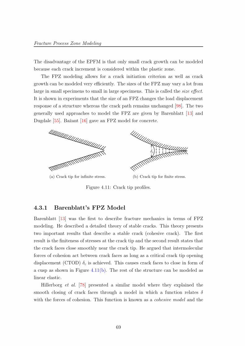
Fracture Process Zone Modeling
The disadvantage of the EPFM is that only small crack growth can be modeled
because each crack increment is considered within the plastic zone.
The FPZ modeling allows for a crack initiation criterion as well as crack
growth can be modeled very efficiently. The sizes of the FPZ may vary a lot from
large in small specimens to small in large specimens. This is called the size effect.
It is shown in experiments that the size of an FPZ changes the load displacement
response of a structure whereas the crack path remains unchanged [98]. The two
generally used approaches to model the FPZ are given by Barenblatt [13] and
Dugdale [55]. Bazant [16] gave an FPZ model for concrete.
(a) Crack tip for infinite stress.
δc
(b) Crack tip for finite stress.
Figure 4.11: Crack tip profiles.
4.3.1 Barenblatt’s FPZ Model
Barenblatt [13] was the first to describe fracture mechanics in terms of FPZ
modeling. He described a detailed theory of stable cracks. This theory presents
two important results that describe a stable crack (cohesive crack). The first
result is the finiteness of stresses at the crack tip and the second result states that
the crack faces close smoothly near the crack tip. He argued that intermolecular
forces of cohesion act between crack faces as long as a critical crack tip opening
displacement (CTOD) δc is achieved. This causes crack faces to close in form of
a cusp as shown in Figure 4.11(b). The rest of the structure can be modeled as
linear elastic.
Hillerborg et al. [78] presented a similar model where they explained the
smooth closing of crack faces through a model in which a function relates δ
with the forces of cohesion. This function is known as a cohesive model and the
69
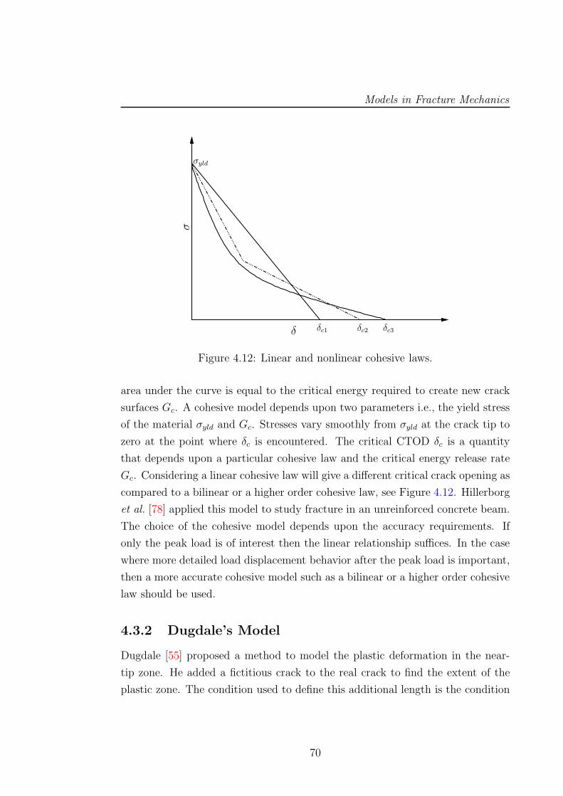
Models in Fracture Mechanics
δc2δ
σ
σyld
δc1 δc3
Figure 4.12: Linear and nonlinear cohesive laws.
area under the curve is equal to the critical energy required to create new crack
surfaces Gc. A cohesive model depends upon two parameters i.e., the yield stress
of the material σyld and Gc. Stresses vary smoothly from σyld at the crack tip to
zero at the point where δc is encountered. The critical CTOD δc is a quantity
that depends upon a particular cohesive law and the critical energy release rate
Gc. Considering a linear cohesive law will give a different critical crack opening as
compared to a bilinear or a higher order cohesive law, see Figure 4.12. Hillerborg
et al. [78] applied this model to study fracture in an unreinforced concrete beam.
The choice of the cohesive model depends upon the accuracy requirements. If
only the peak load is of interest then the linear relationship suffices. In the case
where more detailed load displacement behavior after the peak load is important,
then a more accurate cohesive model such as a bilinear or a higher order cohesive
law should be used.
4.3.2 Dugdale’s Model
Dugdale [55] proposed a method to model the plastic deformation in the near-
tip zone. He added a fictitious crack to the real crack to find the extent of the
plastic zone. The condition used to define this additional length is the condition
70
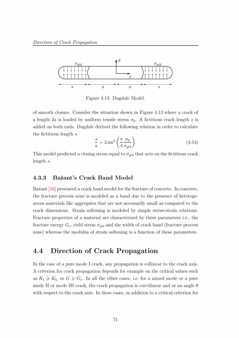
Direction of Crack Propagation
x
y
s a a s
σyldσyld
Figure 4.13: Dugdale Model.
of smooth closure. Consider the situation shown in Figure 4.13 where a crack of
a length 2a is loaded by uniform tensile stress σ0. A fictitious crack length s is
added on both ends. Dugdale derived the following relation in order to calculate
the fictitious length ss
a= 2 sin2
(π
4
σ0σyld
)
. (4.54)
This model predicted a closing stress equal to σyld that acts on the fictitious crack
length s.
4.3.3 Bazant’s Crack Band Model
Bazant [16] presented a crack band model for the fracture of concrete. In concrete,
the fracture process zone is modeled as a band due to the presence of heteroge-
neous materials like aggregates that are not necessarily small as compared to the
crack dimensions. Strain softening is modeled by simple stress-strain relations.
Fracture properties of a material are characterized by three parameters i.e., the
fracture energy Gc, yield stress σyld and the width of crack band (fracture process
zone) whereas the modulus of strain softening is a function of these parameters.
4.4 Direction of Crack Propagation
In the case of a pure mode I crack, any propagation is collinear to the crack axis.
A criterion for crack propagation depends for example on the critical values such
as KI > KIc or G > Gc. In all the other cases, i.e. for a mixed mode or a pure
mode II or mode III crack, the crack propagation is curvilinear and at an angle θ
with respect to the crack axis. In these cases, in addition to a critical criterion for
71
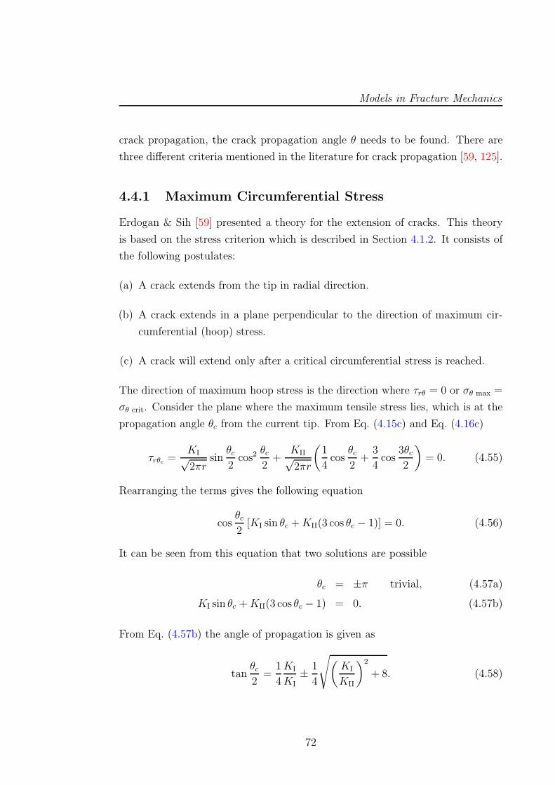
Models in Fracture Mechanics
crack propagation, the crack propagation angle θ needs to be found. There are
three different criteria mentioned in the literature for crack propagation [59, 125].
4.4.1 Maximum Circumferential Stress
Erdogan & Sih [59] presented a theory for the extension of cracks. This theory
is based on the stress criterion which is described in Section 4.1.2. It consists of
the following postulates:
(a) A crack extends from the tip in radial direction.
(b) A crack extends in a plane perpendicular to the direction of maximum cir-
cumferential (hoop) stress.
(c) A crack will extend only after a critical circumferential stress is reached.
The direction of maximum hoop stress is the direction where τrθ = 0 or σθ max =
σθ crit. Consider the plane where the maximum tensile stress lies, which is at the
propagation angle θc from the current tip. From Eq. (4.15c) and Eq. (4.16c)
τrθc =KI√2πr
sinθc2cos2
θc2+
KII√2πr
(1
4cos
θc2+
3
4cos
3θc2
)
= 0. (4.55)
Rearranging the terms gives the following equation
cosθc2[KI sin θc +KII(3 cos θc − 1)] = 0. (4.56)
It can be seen from this equation that two solutions are possible
θc = ±π trivial, (4.57a)
KI sin θc +KII(3 cos θc − 1) = 0. (4.57b)
From Eq. (4.57b) the angle of propagation is given as
tanθc2
=1
4
KI
KI± 1
4
√(KI
KII
)2
+ 8. (4.58)
72
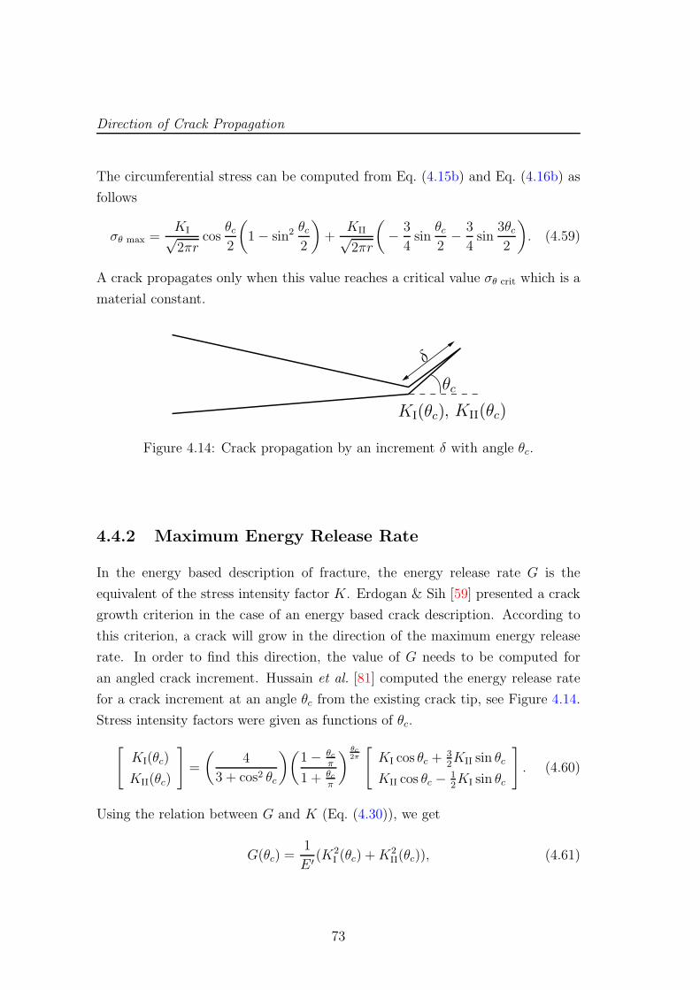
Direction of Crack Propagation
The circumferential stress can be computed from Eq. (4.15b) and Eq. (4.16b) as
follows
σθ max =KI√2πr
cosθc2
(
1− sin2 θc2
)
+KII√2πr
(
− 3
4sin
θc2− 3
4sin
3θc2
)
. (4.59)
A crack propagates only when this value reaches a critical value σθ crit which is a
material constant.
, KII(θc)
δ
θc
KI(θc)
Figure 4.14: Crack propagation by an increment δ with angle θc.
4.4.2 Maximum Energy Release Rate
In the energy based description of fracture, the energy release rate G is the
equivalent of the stress intensity factor K. Erdogan & Sih [59] presented a crack
growth criterion in the case of an energy based crack description. According to
this criterion, a crack will grow in the direction of the maximum energy release
rate. In order to find this direction, the value of G needs to be computed for
an angled crack increment. Hussain et al. [81] computed the energy release rate
for a crack increment at an angle θc from the existing crack tip, see Figure 4.14.
Stress intensity factors were given as functions of θc.
[
KI(θc)
KII(θc)
]
=
(4
3 + cos2 θc
)(1− θc
π
1 + θcπ
) θc2π
[
KI cos θc +32KII sin θc
KII cos θc − 12KI sin θc
]
. (4.60)
Using the relation between G and K (Eq. (4.30)), we get
G(θc) =1
E ′ (K2I (θc) +K2
II(θc)), (4.61)
73
Models in Fracture Mechanics
which gives
G(θc) =4
E ′
(1
3 + cos2 θc
)2(1− θcπ
1 + θcπ
) θc2π
[(1 + 3 cos2 θc)K
2I + 8 sin θc cos θcKIKII + (9− 5 cos2 θc)K
2II
].
(4.62)
In order to find the angle with maximum energy release rate, G(θc) is maximized
as∂G(θc)
∂θc= 0,
∂2G(θc)
∂θ2c< 0. (4.63)
The angle where the maximum energy release rate in the case of pure mode II
(KI = 0) is found to be θc = 70.52.
4.4.3 Minimum Strain Energy Density
Sih [125] explained the crack propagation in terms of strain energy density. He
proposed that a crack propagates in the direction of minimum strain energy
density i.e., the path with the least resistance. Following the description of Sih
[125] the stresses in polar coordinates for a mixed mode fracture are given as
σrr =1√2r
cosθc2
[
KI
(
1 + sin2 θc2
)
+3
2KII sin θc − 2KII tan
θc2
]
.(4.64a)
σθcθc =1√2r
cosθc2
[
KI cos2 θc2− 3
2KII sin θc
]
. (4.64b)
τrθc =1√2r
cosθc2[KI sin θc +KII(3 cos θc − 1)] . (4.64c)
74
Direction of Crack Propagation
Displacements in polar coordinates are given as [125]
ur =1
4
√r
2µ
KI
[(
2κ− 1
)
cosθc2− cos
3θc2
]
−
KII
[(
2κ− 1
)
sinθc2− 3 sin
3θc2
], (4.65a)
uθc =1
4
√r
2µ
KI
[
−(
2κ+ 1
)
sinθc2+ sin
3θc2
]
−
KII
[(
2κ+ 1
)
cosθc2− 3 cos
3θc2
]. (4.65b)
Strain energy density per unit area in terms of polar coordinates is given by
dW
dA=
1
2
[
σr∂ur∂r
+ σθc
(urr
+1
r
∂vθc∂θc
)
+ τrθc
(1
r
∂ur∂θc
+∂vθc∂r
− vθcr
)]
. (4.66)
Introducing the stresses (4.64) and displacements (4.65) in Eq. (4.66) gives the
following equation
dW
dA=
1
r(a11K
2I + 2a12KIKII + a22K
2II), (4.67)
where
a11 =1
16µ[(1 + cos θc)(κ− cos θc)] , (4.68a)
a12 =1
16µsin θc [2 cos θc − (κ− 1)] , (4.68b)
a22 =1
16µ[(κ+ 1)(1− cos θc) + (1 + cos θc)(3 cos θc − 1)] . (4.68c)
The strain energy density per unit area as given by Eq. (4.67) is scaled by the
inverse of the radial distance from the crack tip. The magnitude of this field is
denoted as the strain energy density factor by Sih [125] as
S = a11K2I + 2a12KIKII + a22K
2II. (4.69)
75
Models in Fracture Mechanics
In order to find the propagation direction, this factor is minimized i.e.
∂S(θc)
∂θc= 0,
∂2S(θc)
∂θ2c> 0. (4.70)
A crack is initiated only when the critical value of the strain energy density factor
is reached i.e.,
S = Scr. (4.71)
This critical value is a material constant and found experimentally.
4.5 Outlook
In this chapter, an overview of various models in fracture mechanics is given.
Several crack propagation criteria are discussed. The focus of this work will
remain on linear elastic fracture and fracture process zone modeling. As a crack
propagation criteria, the maximum hoop stress criterion is used. In the next
chapter, numerical fracture mechanics is discussed in the frame of the XFEM.
Hybrid explicit-implicit crack representation is given for 2D and 3D fracture which
is used in a crack propagation scheme. The XFEM approximation is explained
and then the HG-XFEM for fracture mechanics is discussed.
76
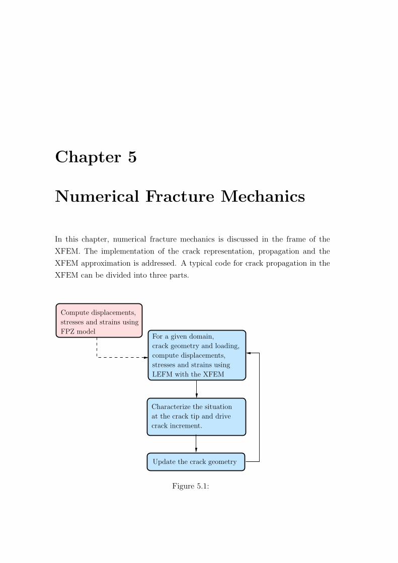
Chapter 5
Numerical Fracture Mechanics
In this chapter, numerical fracture mechanics is discussed in the frame of the
XFEM. The implementation of the crack representation, propagation and the
XFEM approximation is addressed. A typical code for crack propagation in the
XFEM can be divided into three parts.
FPZ modelFor a given domain,
crack geometry and loading,
compute displacements,
stresses and strains using
LEFM with the XFEM
Characterize the situation
at the crack tip and drive
crack increment.
Update the crack geometry
Compute displacements,
stresses and strains using
Figure 5.1:
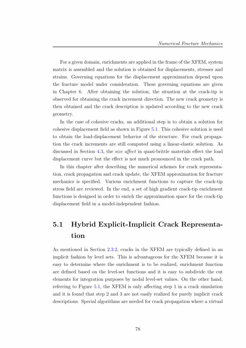
Numerical Fracture Mechanics
For a given domain, enrichments are applied in the frame of the XFEM, system
matrix is assembled and the solution is obtained for displacements, stresses and
strains. Governing equations for the displacement approximation depend upon
the fracture model under consideration. These governing equations are given
in Chapter 6. After obtaining the solution, the situation at the crack-tip is
observed for obtaining the crack increment direction. The new crack geometry is
then obtained and the crack description is updated according to the new crack
geometry.
In the case of cohesive cracks, an additional step is to obtain a solution for
cohesive displacement field as shown in Figure 5.1. This cohesive solution is used
to obtain the load-displacement behavior of the structure. For crack propaga-
tion the crack increments are still computed using a linear-elastic solution. As
discussed in Section 4.3, the size affect in quasi-brittle materials effect the load
displacement curve but the effect is not much pronounced in the crack path.
In this chapter after describing the numerical schemes for crack representa-
tion, crack propagation and crack update, the XFEM approximation for fracture
mechanics is specified. Various enrichment functions to capture the crack-tip
stress field are reviewed. In the end, a set of high gradient crack-tip enrichment
functions is designed in order to enrich the approximation space for the crack-tip
displacement field in a model-independent fashion.
5.1 Hybrid Explicit-Implicit Crack Representa-
tion
As mentioned in Section 2.3.2, cracks in the XFEM are typically defined in an
implicit fashion by level sets. This is advantageous for the XFEM because it is
easy to determine where the enrichment is to be realized, enrichment function
are defined based on the level-set functions and it is easy to subdivide the cut
elements for integration purposes by nodal level-set values. On the other hand,
referring to Figure 5.1, the XFEM is only affecting step 1 in a crack simulation
and it is found that step 2 and 3 are not easily realized for purely implicit crack
descriptions. Special algorithms are needed for crack propagation where a virtual
78
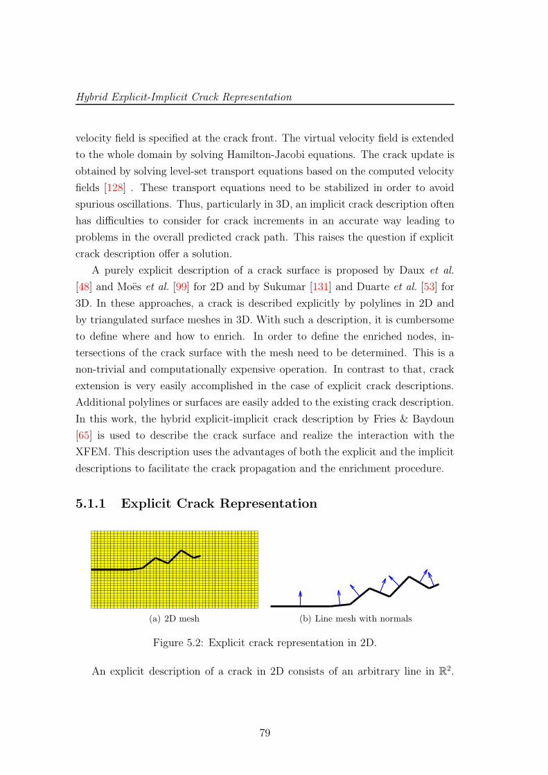
Hybrid Explicit-Implicit Crack Representation
velocity field is specified at the crack front. The virtual velocity field is extended
to the whole domain by solving Hamilton-Jacobi equations. The crack update is
obtained by solving level-set transport equations based on the computed velocity
fields [128] . These transport equations need to be stabilized in order to avoid
spurious oscillations. Thus, particularly in 3D, an implicit crack description often
has difficulties to consider for crack increments in an accurate way leading to
problems in the overall predicted crack path. This raises the question if explicit
crack description offer a solution.
A purely explicit description of a crack surface is proposed by Daux et al.
[48] and Moes et al. [99] for 2D and by Sukumar [131] and Duarte et al. [53] for
3D. In these approaches, a crack is described explicitly by polylines in 2D and
by triangulated surface meshes in 3D. With such a description, it is cumbersome
to define where and how to enrich. In order to define the enriched nodes, in-
tersections of the crack surface with the mesh need to be determined. This is a
non-trivial and computationally expensive operation. In contrast to that, crack
extension is very easily accomplished in the case of explicit crack descriptions.
Additional polylines or surfaces are easily added to the existing crack description.
In this work, the hybrid explicit-implicit crack description by Fries & Baydoun
[65] is used to describe the crack surface and realize the interaction with the
XFEM. This description uses the advantages of both the explicit and the implicit
descriptions to facilitate the crack propagation and the enrichment procedure.
5.1.1 Explicit Crack Representation
(a) 2D mesh (b) Line mesh with normals
Figure 5.2: Explicit crack representation in 2D.
An explicit description of a crack in 2D consists of an arbitrary line in R2.
79
Numerical Fracture Mechanics
This line is discretized into straight line segments where each line segment is
a straight element of a 1D mesh in R2. Each element consists of two nodes.
Elements are defined in a connectivity matrix where the nodes are connected in
such a way that a consistent direction of normals in each element is obtained.
The line mesh and the direction of normals in each segment for a 2D crack are
shown in Figure 5.2(b). In the case of a 2D crack that is not fully immersed into
the domain e.g. edge cracks, the line mesh has two tips but only one tip is active,
see Figure 5.2(a). This information is given by another variable that specifies the
nodes that are active tip nodes. As it shall be seen later that the extension of
the crack path in tangential direction at each active crack tip is a crucial part
of the hybrid explicit-implicit crack description. In order to get this extension a
coordinate system is defined at each active crack tip, see Fries & Baydoun [65] for
the details on computing this coordinate system. A crack tip coordinate system
for an edge crack with only one active crack tip is shown in Figure 5.3. The crack
path is extended by adding a line segment in the tangential direction with length
l → ∞. This length in practice is a large number about ten times larger than
the maximum length scale of the domain. The additional line segment is added
such that the normal direction in the additional segment is consistent with the
original crack. See Figure 5.11(a) for the crack extension in the case of an edge
crack.
Figure 5.3: Crack tip coordinate system.
An explicit description of a crack in 3D consists of an arbitrary hypersurface
in R3. The arbitrary hypersurface is discretized into flat triangles where each
triangle is an element of a 2D mesh described in R3. Each element consists of
three nodes. The connectivity matrix is defined similar to the 2D case where
the nodes are connected in such a way that a consistent direction of normals
in each element is obtained. Consider a 3D crack represented by a triangulated
surface mesh as shown in Figure 5.4. In this case, the triangular mesh and the
80
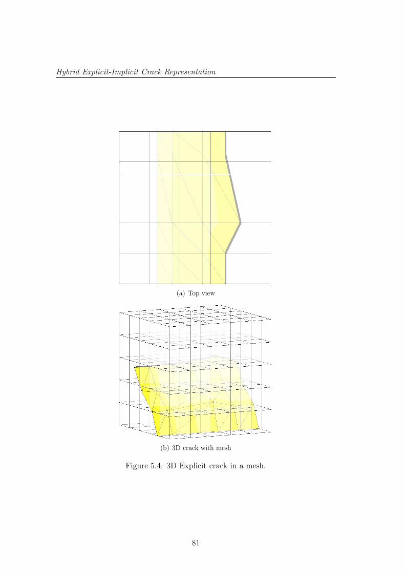
Hybrid Explicit-Implicit Crack Representation
(a) Top view
(b) 3D crack with mesh
Figure 5.4: 3D Explicit crack in a mesh.
81
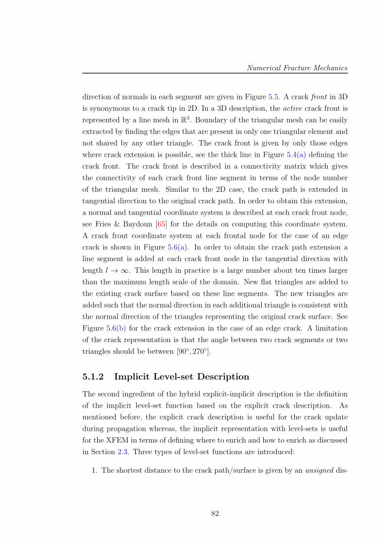
Numerical Fracture Mechanics
direction of normals in each segment are given in Figure 5.5. A crack front in 3D
is synonymous to a crack tip in 2D. In a 3D description, the active crack front is
represented by a line mesh in R3. Boundary of the triangular mesh can be easily
extracted by finding the edges that are present in only one triangular element and
not shared by any other triangle. The crack front is given by only those edges
where crack extension is possible, see the thick line in Figure 5.4(a) defining the
crack front. The crack front is described in a connectivity matrix which gives
the connectivity of each crack front line segment in terms of the node number
of the triangular mesh. Similar to the 2D case, the crack path is extended in
tangential direction to the original crack path. In order to obtain this extension,
a normal and tangential coordinate system is described at each crack front node,
see Fries & Baydoun [65] for the details on computing this coordinate system.
A crack front coordinate system at each frontal node for the case of an edge
crack is shown in Figure 5.6(a). In order to obtain the crack path extension a
line segment is added at each crack front node in the tangential direction with
length l → ∞. This length in practice is a large number about ten times larger
than the maximum length scale of the domain. New flat triangles are added to
the existing crack surface based on these line segments. The new triangles are
added such that the normal direction in each additional triangle is consistent with
the normal direction of the triangles representing the original crack surface. See
Figure 5.6(b) for the crack extension in the case of an edge crack. A limitation
of the crack representation is that the angle between two crack segments or two
triangles should be between [90, 270].
5.1.2 Implicit Level-set Description
The second ingredient of the hybrid explicit-implicit description is the definition
of the implicit level-set function based on the explicit crack description. As
mentioned before, the explicit crack description is useful for the crack update
during propagation whereas, the implicit representation with level-sets is useful
for the XFEM in terms of defining where to enrich and how to enrich as discussed
in Section 2.3. Three types of level-set functions are introduced:
1. The shortest distance to the crack path/surface is given by an unsigned dis-
82
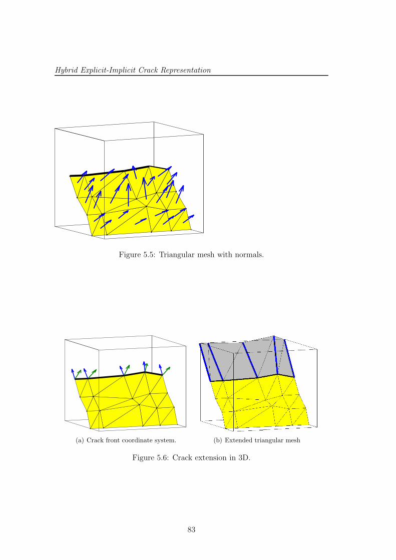
Hybrid Explicit-Implicit Crack Representation
Figure 5.5: Triangular mesh with normals.
(a) Crack front coordinate system. (b) Extended triangular mesh
Figure 5.6: Crack extension in 3D.
83
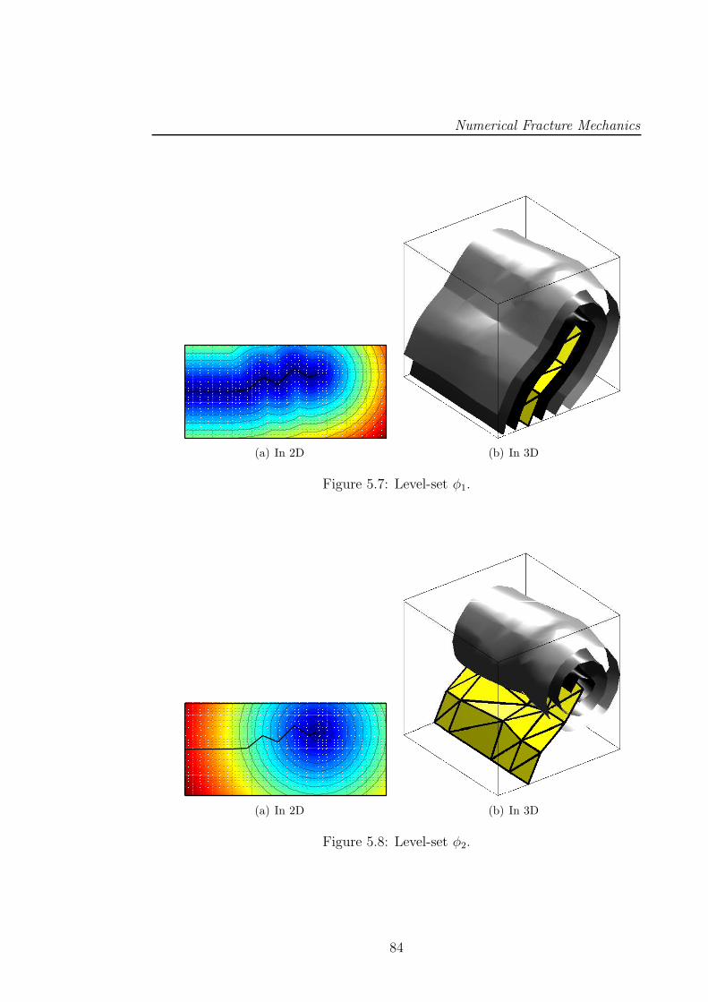
Numerical Fracture Mechanics
(a) In 2D (b) In 3D
Figure 5.7: Level-set φ1.
(a) In 2D (b) In 3D
Figure 5.8: Level-set φ2.
84
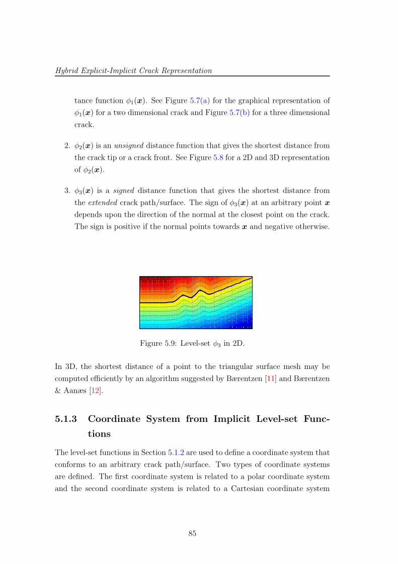
Hybrid Explicit-Implicit Crack Representation
tance function φ1(x). See Figure 5.7(a) for the graphical representation of
φ1(x) for a two dimensional crack and Figure 5.7(b) for a three dimensional
crack.
2. φ2(x) is an unsigned distance function that gives the shortest distance from
the crack tip or a crack front. See Figure 5.8 for a 2D and 3D representation
of φ2(x).
3. φ3(x) is a signed distance function that gives the shortest distance from
the extended crack path/surface. The sign of φ3(x) at an arbitrary point x
depends upon the direction of the normal at the closest point on the crack.
The sign is positive if the normal points towards x and negative otherwise.
Figure 5.9: Level-set φ3 in 2D.
In 3D, the shortest distance of a point to the triangular surface mesh may be
computed efficiently by an algorithm suggested by Bærentzen [11] and Bærentzen
& Aanæs [12].
5.1.3 Coordinate System from Implicit Level-set Func-
tions
The level-set functions in Section 5.1.2 are used to define a coordinate system that
conforms to an arbitrary crack path/surface. Two types of coordinate systems
are defined. The first coordinate system is related to a polar coordinate system
and the second coordinate system is related to a Cartesian coordinate system
85
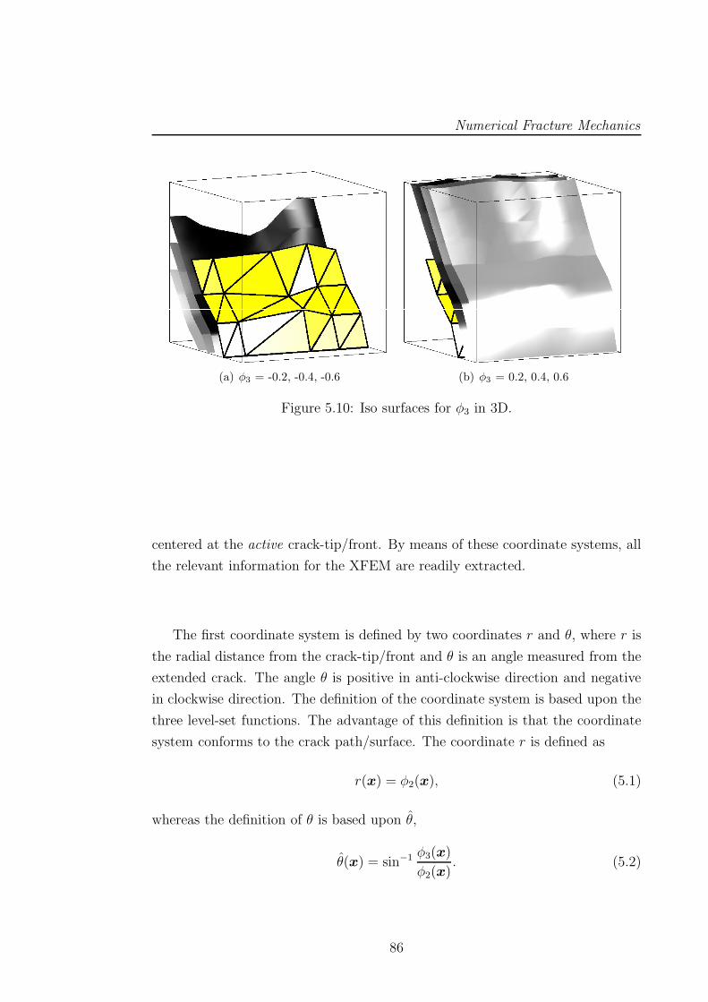
Numerical Fracture Mechanics
(a) φ3 = -0.2, -0.4, -0.6 (b) φ3 = 0.2, 0.4, 0.6
Figure 5.10: Iso surfaces for φ3 in 3D.
centered at the active crack-tip/front. By means of these coordinate systems, all
the relevant information for the XFEM are readily extracted.
The first coordinate system is defined by two coordinates r and θ, where r is
the radial distance from the crack-tip/front and θ is an angle measured from the
extended crack. The angle θ is positive in anti-clockwise direction and negative
in clockwise direction. The definition of the coordinate system is based upon the
three level-set functions. The advantage of this definition is that the coordinate
system conforms to the crack path/surface. The coordinate r is defined as
r(x) = φ2(x), (5.1)
whereas the definition of θ is based upon θ,
θ(x) = sin−1 φ3(x)
φ2(x). (5.2)
86
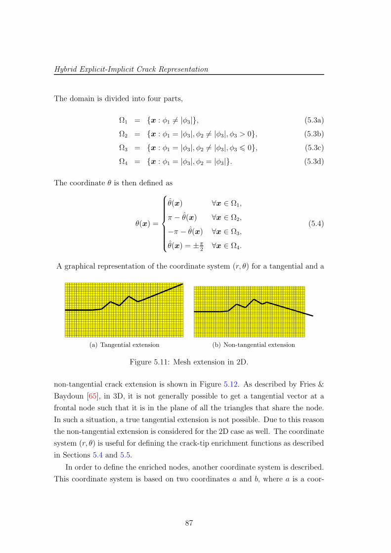
Hybrid Explicit-Implicit Crack Representation
The domain is divided into four parts,
Ω1 = x : φ1 6= |φ3|, (5.3a)
Ω2 = x : φ1 = |φ3|, φ2 6= |φ3|, φ3 > 0, (5.3b)
Ω3 = x : φ1 = |φ3|, φ2 6= |φ3|, φ3 6 0, (5.3c)
Ω4 = x : φ1 = |φ3|, φ2 = |φ3|. (5.3d)
The coordinate θ is then defined as
θ(x) =
θ(x) ∀x ∈ Ω1,
π − θ(x) ∀x ∈ Ω2,
−π − θ(x) ∀x ∈ Ω3,
θ(x) = ±π2
∀x ∈ Ω4.
(5.4)
A graphical representation of the coordinate system (r, θ) for a tangential and a
(a) Tangential extension (b) Non-tangential extension
Figure 5.11: Mesh extension in 2D.
non-tangential crack extension is shown in Figure 5.12. As described by Fries &
Baydoun [65], in 3D, it is not generally possible to get a tangential vector at a
frontal node such that it is in the plane of all the triangles that share the node.
In such a situation, a true tangential extension is not possible. Due to this reason
the non-tangential extension is considered for the 2D case as well. The coordinate
system (r, θ) is useful for defining the crack-tip enrichment functions as described
in Sections 5.4 and 5.5.
In order to define the enriched nodes, another coordinate system is described.
This coordinate system is based on two coordinates a and b, where a is a coor-
87
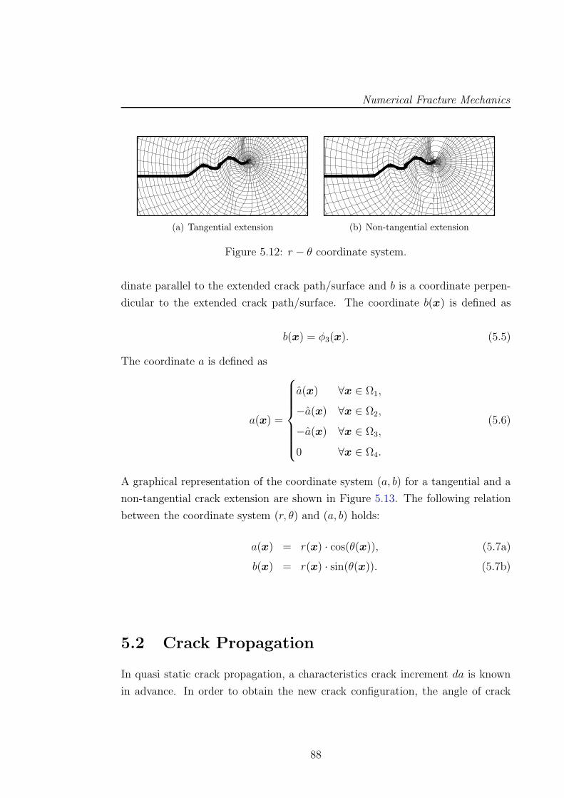
Numerical Fracture Mechanics
(a) Tangential extension (b) Non-tangential extension
Figure 5.12: r − θ coordinate system.
dinate parallel to the extended crack path/surface and b is a coordinate perpen-
dicular to the extended crack path/surface. The coordinate b(x) is defined as
b(x) = φ3(x). (5.5)
The coordinate a is defined as
a(x) =
a(x) ∀x ∈ Ω1,
−a(x) ∀x ∈ Ω2,
−a(x) ∀x ∈ Ω3,
0 ∀x ∈ Ω4.
(5.6)
A graphical representation of the coordinate system (a, b) for a tangential and a
non-tangential crack extension are shown in Figure 5.13. The following relation
between the coordinate system (r, θ) and (a, b) holds:
a(x) = r(x) · cos(θ(x)), (5.7a)
b(x) = r(x) · sin(θ(x)). (5.7b)
5.2 Crack Propagation
In quasi static crack propagation, a characteristics crack increment da is known
in advance. In order to obtain the new crack configuration, the angle of crack
88
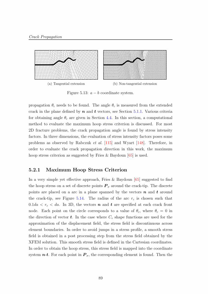
Crack Propagation
(a) Tangential extension (b) Non-tangential extension
Figure 5.13: a− b coordinate system.
propagation θc needs to be found. The angle θc is measured from the extended
crack in the plane defined by n and t vectors, see Section 5.1.1. Various criteria
for obtaining angle θc are given in Section 4.4. In this section, a computational
method to evaluate the maximum hoop stress criterion is discussed. For most
2D fracture problems, the crack propagation angle is found by stress intensity
factors. In three dimensions, the evaluation of stress intensity factors poses some
problems as observed by Rabczuk et al. [115] and Wyart [148]. Therefore, in
order to evaluate the crack propagation direction in this work, the maximum
hoop stress criterion as suggested by Fries & Baydoun [65] is used.
5.2.1 Maximum Hoop Stress Criterion
In a very simple yet effective approach, Fries & Baydoun [65] suggested to find
the hoop stress on a set of discrete points P σ around the crack-tip. The discrete
points are placed on a arc in a plane spanned by the vectors n and t around
the crack-tip, see Figure 5.14. The radius of the arc rc is chosen such that
0.1da < rc < da. In 3D, the vectors n and t are specified at each crack front
node. Each point on the circle corresponds to a value of θc, where θc = 0 in
the direction of vector t. In the case where C shape functions are used for the
approximation of the displacement field, the stress field is discontinuous across
element boundaries. In order to avoid jumps in a stress profile, a smooth stress
field is obtained in a post processing step from the stress field obtained by the
XFEM solution. This smooth stress field is defined in the Cartesian coordinates.
In order to obtain the hoop stress, this stress field is mapped into the coordinate
system n-t. For each point in P σ, the corresponding element is found. Then the
89
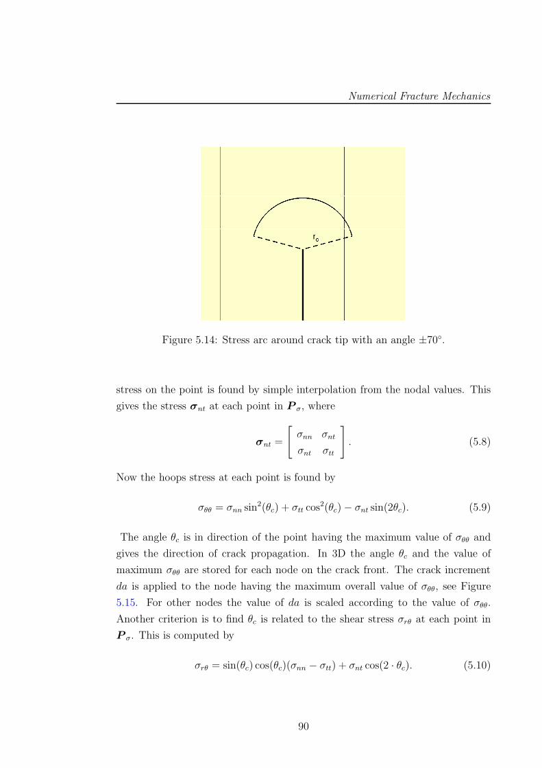
Numerical Fracture Mechanics
Figure 5.14: Stress arc around crack tip with an angle ±70.
stress on the point is found by simple interpolation from the nodal values. This
gives the stress σnt at each point in P σ, where
σnt =
[
σnn σnt
σnt σtt
]
. (5.8)
Now the hoops stress at each point is found by
σθθ = σnn sin2(θc) + σtt cos
2(θc)− σnt sin(2θc). (5.9)
The angle θc is in direction of the point having the maximum value of σθθ and
gives the direction of crack propagation. In 3D the angle θc and the value of
maximum σθθ are stored for each node on the crack front. The crack increment
da is applied to the node having the maximum overall value of σθθ, see Figure
5.15. For other nodes the value of da is scaled according to the value of σθθ.
Another criterion is to find θc is related to the shear stress σrθ at each point in
P σ. This is computed by
σrθ = sin(θc) cos(θc)(σnn − σtt) + σnt cos(2 · θc). (5.10)
90
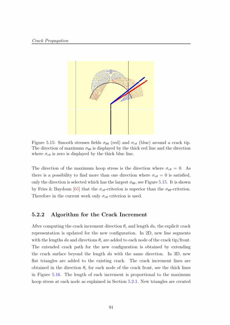
Crack Propagation
Figure 5.15: Smooth stresses fields σθθ (red) and σrθ (blue) around a crack tip.The direction of maximum σθθ is displayed by the thick red line and the directionwhere σrθ is zero is displayed by the thick blue line.
The direction of the maximum hoop stress is the direction where σrθ = 0. As
there is a possibility to find more than one direction where σrθ = 0 is satisfied,
only the direction is selected which has the largest σθθ, see Figure 5.15. It is shown
by Fries & Baydoun [65] that the σrθ-criterion is superior than the σθθ-criterion.
Therefore in the current work only σrθ criterion is used.
5.2.2 Algorithm for the Crack Increment
After computing the crack increment direction θc and length da, the explicit crack
representation is updated for the new configuration. In 2D, new line segments
with the lengths da and directions θc are added to each node of the crack tip/front.
The extended crack path for the new configuration is obtained by extending
the crack surface beyond the length da with the same direction. In 3D, new
flat triangles are added to the existing crack. The crack increment lines are
obtained in the direction θc for each node of the crack front, see the thick lines
in Figure 5.16. The length of each increment is proportional to the maximum
hoop stress at each node as explained in Section 5.2.1. New triangles are created
91
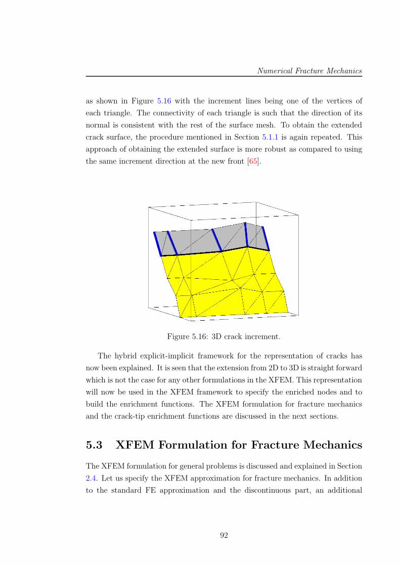
Numerical Fracture Mechanics
as shown in Figure 5.16 with the increment lines being one of the vertices of
each triangle. The connectivity of each triangle is such that the direction of its
normal is consistent with the rest of the surface mesh. To obtain the extended
crack surface, the procedure mentioned in Section 5.1.1 is again repeated. This
approach of obtaining the extended surface is more robust as compared to using
the same increment direction at the new front [65].
Figure 5.16: 3D crack increment.
The hybrid explicit-implicit framework for the representation of cracks has
now been explained. It is seen that the extension from 2D to 3D is straight forward
which is not the case for any other formulations in the XFEM. This representation
will now be used in the XFEM framework to specify the enriched nodes and to
build the enrichment functions. The XFEM formulation for fracture mechanics
and the crack-tip enrichment functions are discussed in the next sections.
5.3 XFEM Formulation for Fracture Mechanics
The XFEM formulation for general problems is discussed and explained in Section
2.4. Let us specify the XFEM approximation for fracture mechanics. In addition
to the standard FE approximation and the discontinuous part, an additional
92
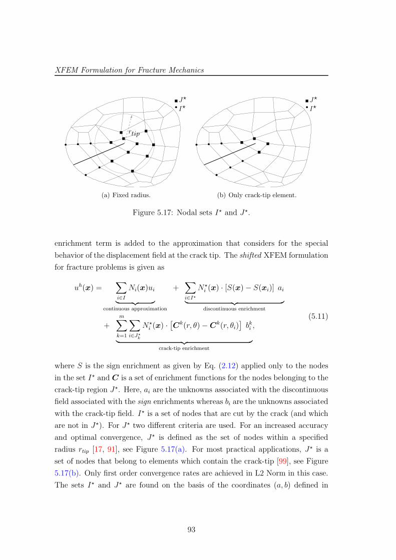
XFEM Formulation for Fracture Mechanics
rtip
J⋆
I⋆
(a) Fixed radius.
I⋆J⋆
(b) Only crack-tip element.
Figure 5.17: Nodal sets I⋆ and J⋆.
enrichment term is added to the approximation that considers for the special
behavior of the displacement field at the crack tip. The shifted XFEM formulation
for fracture problems is given as
uh(x) =∑
i∈I
Ni(x)ui
︸ ︷︷ ︸
continuous approximation
+∑
i∈I⋆N⋆
i (x) · [S(x)− S(xi)] ai
︸ ︷︷ ︸
discontinuous enrichment
+
m∑
k=1
∑
i∈J⋆k
N⋆i (x) ·
[Ck(r, θ)−Ck(r, θi)
]bki
︸ ︷︷ ︸
crack-tip enrichment
,(5.11)
where S is the sign enrichment as given by Eq. (2.12) applied only to the nodes
in the set I⋆ and C is a set of enrichment functions for the nodes belonging to the
crack-tip region J⋆. Here, ai are the unknowns associated with the discontinuous
field associated with the sign enrichments whereas bi are the unknowns associated
with the crack-tip field. I⋆ is a set of nodes that are cut by the crack (and which
are not in J⋆). For J⋆ two different criteria are used. For an increased accuracy
and optimal convergence, J⋆ is defined as the set of nodes within a specified
radius rtip [17, 91], see Figure 5.17(a). For most practical applications, J⋆ is a
set of nodes that belong to elements which contain the crack-tip [99], see Figure
5.17(b). Only first order convergence rates are achieved in L2 Norm in this case.
The sets I⋆ and J⋆ are found on the basis of the coordinates (a, b) defined in
93
Numerical Fracture Mechanics
Section 5.1.3. If a domain is divided into n elements and Ik denotes all the nodes
of element k then the set J⋆ is defined as
J⋆ =⋃
k∈Ntip
Ik, (5.12)
where Ntip is an element set defined as
Ntip =N
1tip
⋃
N2tip
, (5.13)
where
N1tip =
mini∈Ik
(a(xi)) ·maxi∈Ik
(a(xi)) < 0 and mini∈Ik
(b(xi)) ·maxi∈Ik
(b(xi)) < 0, (5.14)
and
N2tip =
mini∈Ik
(r(xi)) 6 rtip. (5.15)
The set I⋆ is defined as
I⋆ =
⋃
k∈Nstep
Ik
\ J⋆, (5.16)
where
Nstep =maxi∈Ik
(a(xi)) < 0 and mini∈Ik
(b(xi)) ·maxi∈Ik
(b(xi)) < 0\ Ntip. (5.17)
The crack-tip enrichment functions are designed to capture the singular fields
at the crack-tip. These near tip fields have different characteristics for different
fracture models. Thus for each particular fracture model, different crack-tip en-
richment functions are required. In order to design an appropriate enrichment
function for each model, asymptotic near-tip fields need to be investigated. Crack-
tip enrichment functions are based on these asymptotic fields. These enrichment
functions are named “asymptotic crack-tip enrichment” functions in this work.
Asymptotic crack-tip enrichment functions for various models are discussed in
the next section.
94
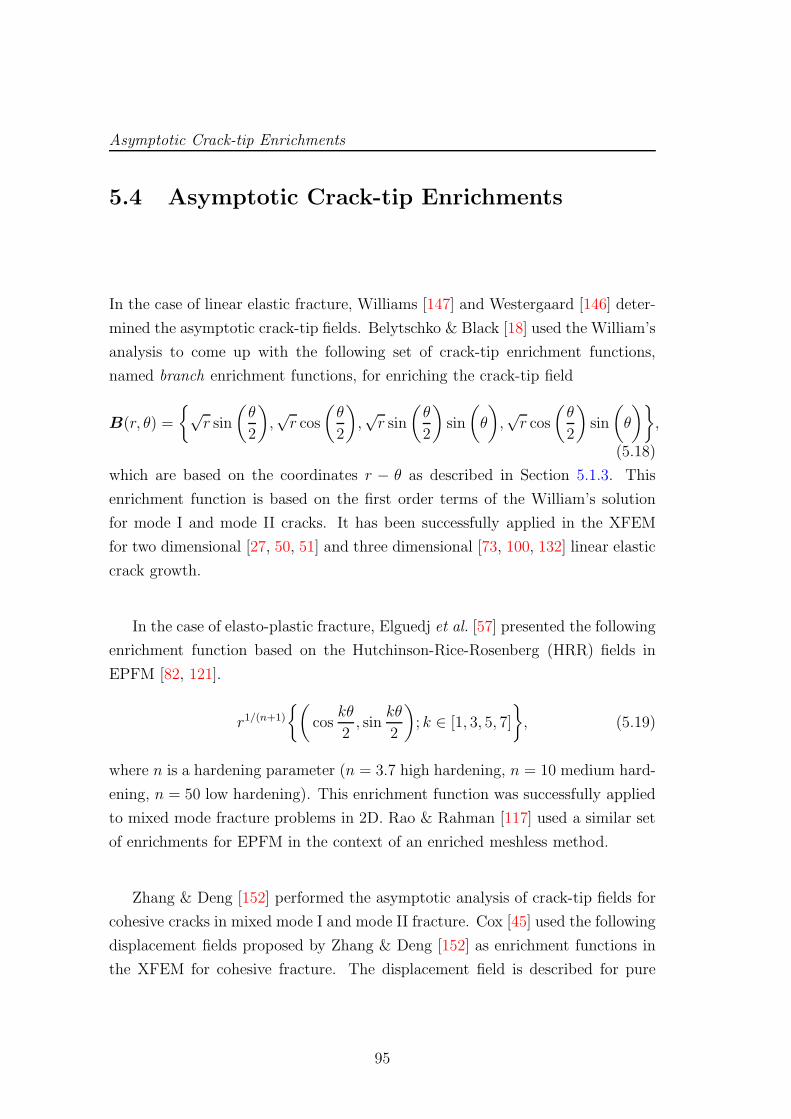
Asymptotic Crack-tip Enrichments
5.4 Asymptotic Crack-tip Enrichments
In the case of linear elastic fracture, Williams [147] and Westergaard [146] deter-
mined the asymptotic crack-tip fields. Belytschko & Black [18] used the William’s
analysis to come up with the following set of crack-tip enrichment functions,
named branch enrichment functions, for enriching the crack-tip field
B(r, θ) =
√r sin
(θ
2
)
,√r cos
(θ
2
)
,√r sin
(θ
2
)
sin
(
θ
)
,√r cos
(θ
2
)
sin
(
θ
)
,
(5.18)
which are based on the coordinates r − θ as described in Section 5.1.3. This
enrichment function is based on the first order terms of the William’s solution
for mode I and mode II cracks. It has been successfully applied in the XFEM
for two dimensional [27, 50, 51] and three dimensional [73, 100, 132] linear elastic
crack growth.
In the case of elasto-plastic fracture, Elguedj et al. [57] presented the following
enrichment function based on the Hutchinson-Rice-Rosenberg (HRR) fields in
EPFM [82, 121].
r1/(n+1)
(
coskθ
2, sin
kθ
2
)
; k ∈ [1, 3, 5, 7]
, (5.19)
where n is a hardening parameter (n = 3.7 high hardening, n = 10 medium hard-
ening, n = 50 low hardening). This enrichment function was successfully applied
to mixed mode fracture problems in 2D. Rao & Rahman [117] used a similar set
of enrichments for EPFM in the context of an enriched meshless method.
Zhang & Deng [152] performed the asymptotic analysis of crack-tip fields for
cohesive cracks in mixed mode I and mode II fracture. Cox [45] used the following
displacement fields proposed by Zhang & Deng [152] as enrichment functions in
the XFEM for cohesive fracture. The displacement field is described for pure
95
Numerical Fracture Mechanics
Figure 5.18: Coordinates w1 and w2 (Figure taken from Cox [45]).
mode I loading as:
u =bc
14035ew1/2 [(2κ− 1) cos(w2/2)− cos(3w2/2)] (5.20a)
− 7e−3w1/2 [5 cos(w2/2)− 4κ cos(3w2/2)− cos(7w2/2)]
+ e−7w1/2 [7 cos(3w2/2)− (2κ+ 5) cos(7w2/2)],
v =bc
14035ew1/2 [(2κ+ 1) sin(w2/2)− sin(3w2/2)] (5.20b)
+ 7e−3w1/2 [5 sin(w2/2)− 4κ sin(3w2/2) + sin(7w2/2)]
+ e−7w1/2 [7 sin(3w2/2) + (2κ− 5) sin(7w2/2)],
and for pure mode II loading as:
u =bc
14035ew1/2 [(2κ+ 3) sin(w2/2) + sin(3w2/2)] (5.21a)
− 7e−3w1/2 [5 sin(w2/2) + 4(κ+ 2) sin(3w2/2) + sin(7w2/2)]
− e−7w1/2 [7 sin(3w2/2)− (2κ+ 9) sin(7w2/2)],
v =− bc
14035ew1/2 [(2κ− 3) cos(w2/2) + cos(3w2/2)] (5.21b)
+ 7e−3w1/2 [5 cos(w2/2) + 4(κ− 2) cos(3w2/2)− cos(7w2/2)]
− e−7w1/2 [7 cos(3w2/2) + (2κ− 9) cos(7w2/2)],
where b is an arbitrary parameter, c is the half the length of the cohesive zone,
see Figure 5.19 and w1 and w2 are the elliptical coordinates (see Figure 5.18)
96
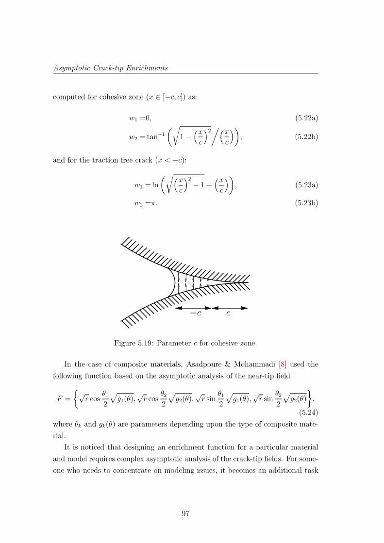
Asymptotic Crack-tip Enrichments
computed for cohesive zone (x ∈ [−c, c]) as:
w1 =0, (5.22a)
w2 =tan−1
(√
1−(x
c
)2/(x
c
))
, (5.22b)
and for the traction free crack (x < −c):
w1 = ln
(√(x
c
)2
− 1−(x
c
))
, (5.23a)
w2 =π. (5.23b)
−c c
Figure 5.19: Parameter c for cohesive zone.
In the case of composite materials, Asadpoure & Mohammadi [8] used the
following function based on the asymptotic analysis of the near-tip field
F =
√r cos
θ12
√
g1(θ),√r cos
θ22
√
g2(θ),√r sin
θ12
√
g1(θ),√r sin
θ22
√
g2(θ)
,
(5.24)
where θk and gk(θ) are parameters depending upon the type of composite mate-
rial.
It is noticed that designing an enrichment function for a particular material
and model requires complex asymptotic analysis of the crack-tip fields. For some-
one who needs to concentrate on modeling issues, it becomes an additional task
97
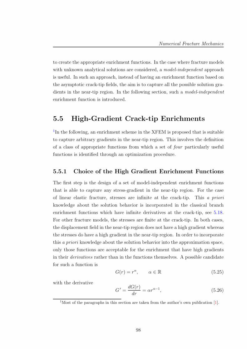
Numerical Fracture Mechanics
to create the appropriate enrichment functions. In the case where fracture models
with unknown analytical solutions are considered, a model-independent approach
is useful. In such an approach, instead of having an enrichment function based on
the asymptotic crack-tip fields, the aim is to capture all the possible solution gra-
dients in the near-tip region. In the following section, such a model-independent
enrichment function is introduced.
5.5 High-Gradient Crack-tip Enrichments
1In the following, an enrichment scheme in the XFEM is proposed that is suitable
to capture arbitrary gradients in the near-tip region. This involves the definition
of a class of appropriate functions from which a set of four particularly useful
functions is identified through an optimization procedure.
5.5.1 Choice of the High Gradient Enrichment Functions
The first step is the design of a set of model-independent enrichment functions
that is able to capture any stress-gradient in the near-tip region. For the case
of linear elastic fracture, stresses are infinite at the crack-tip. This a priori
knowledge about the solution behavior is incorporated in the classical branch
enrichment functions which have infinite derivatives at the crack-tip, see 5.18.
For other fracture models, the stresses are finite at the crack-tip. In both cases,
the displacement field in the near-tip region does not have a high gradient whereas
the stresses do have a high gradient in the near-tip region. In order to incorporate
this a priori knowledge about the solution behavior into the approximation space,
only those functions are acceptable for the enrichment that have high gradients
in their derivatives rather than in the functions themselves. A possible candidate
for such a function is
G(r) = rα, α ∈ R (5.25)
with the derivative
G ′ =dG(r)
dr= αrα−1, (5.26)
1Most of the paragraphs in this section are taken from the author’s own publication [1].
98
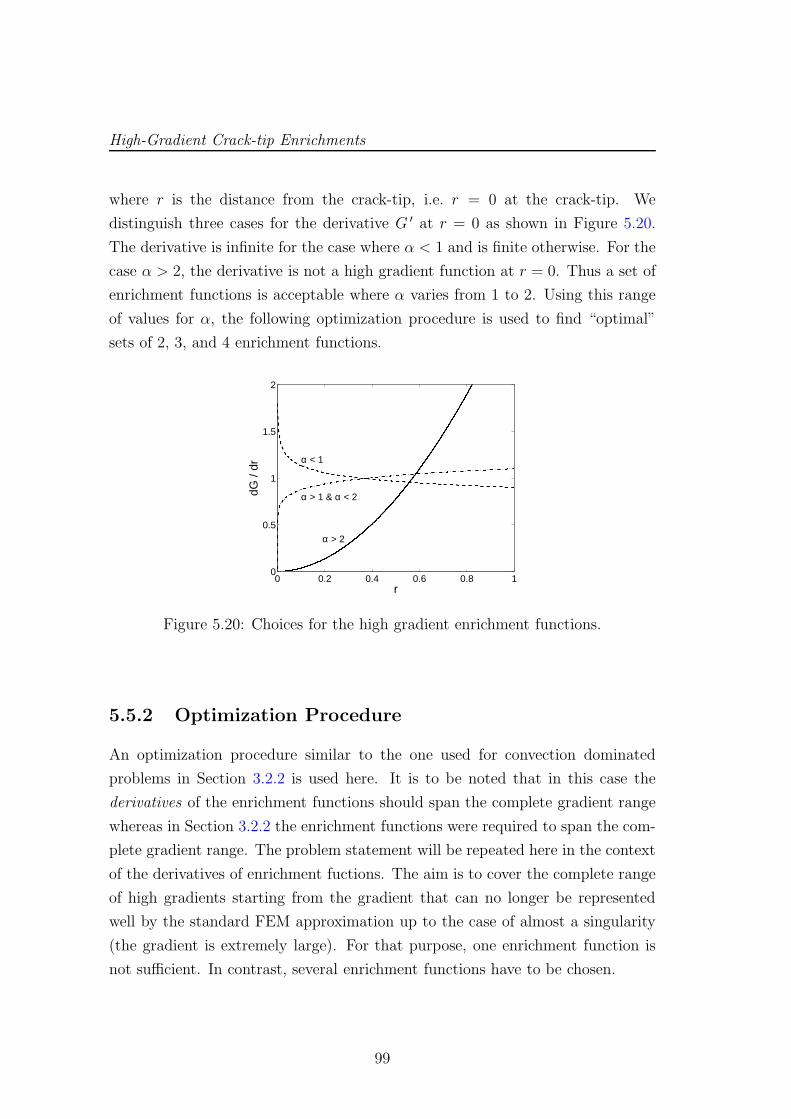
High-Gradient Crack-tip Enrichments
where r is the distance from the crack-tip, i.e. r = 0 at the crack-tip. We
distinguish three cases for the derivative G ′ at r = 0 as shown in Figure 5.20.
The derivative is infinite for the case where α < 1 and is finite otherwise. For the
case α > 2, the derivative is not a high gradient function at r = 0. Thus a set of
enrichment functions is acceptable where α varies from 1 to 2. Using this range
of values for α, the following optimization procedure is used to find “optimal”
sets of 2, 3, and 4 enrichment functions.
0 0.2 0.4 0.6 0.8 10
0.5
1
1.5
2
r
dG /
dr
α > 2
α > 1 & α < 2
α < 1
Figure 5.20: Choices for the high gradient enrichment functions.
5.5.2 Optimization Procedure
An optimization procedure similar to the one used for convection dominated
problems in Section 3.2.2 is used here. It is to be noted that in this case the
derivatives of the enrichment functions should span the complete gradient range
whereas in Section 3.2.2 the enrichment functions were required to span the com-
plete gradient range. The problem statement will be repeated here in the context
of the derivatives of enrichment fuctions. The aim is to cover the complete range
of high gradients starting from the gradient that can no longer be represented
well by the standard FEM approximation up to the case of almost a singularity
(the gradient is extremely large). For that purpose, one enrichment function is
not sufficient. In contrast, several enrichment functions have to be chosen.
99
Numerical Fracture Mechanics
For a given number of m functions
G ′(r) = G ′1(r), . . . , G
′m(r) = α1 · rα1−1, . . . , αm · rαm−1, (5.27)
an optimization procedure is employed in order to determine the corresponding
values α1, . . . , αm. The aim is to minimize the largest point wise error
ε(G ′) = sup(uh(r)− f(r)), (5.28)
of the following interpolation problem
∫
Ω
G ′ uh(r) =
∫
Ω
G ′ f(r), (5.29)
where f can in principle, be any given function having a high gradient in the
near-tip region, i.e. at r = 0. In the current study, the following function f(r) is
chosen that is interpolated by the m functions of Eq. (5.26)
f(r) = G ′(r) = αrα−1. (5.30)
The approximate solution uh(r) of the interpolated function f(r) is given by a
linear combination of interpolator G ′j and the solution uhj , i.e.
uh(r) =m∑
j=1
G ′j · uhj . (5.31)
An important point is that for each prescribed set of enrichment functions G ′,
the gradient of the function f(r) is varied systematically between a minimum
and a maximum gradient by varying the value of α in Eq. (5.30). For each set
G ′, the largest value for ε is stored in εtotal. The optimal set for each number
m is then the one with the smallest εtotal. In this way, optimal sets of two, three
and four enrichment functions are found, see Table 5.1. These functions can
interpolate all the near-tip stress gradients with some accuracy. The accuracy of
the approximation increases with the number of enrichment functions but it is
also noted that the condition number for the stiffness matrix increases with an
100
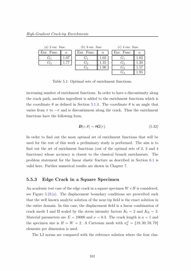
High-Gradient Crack-tip Enrichments
(a) 2 enr. func.
Enr. Func. α
G1 1.07G2 1.77
(b) 3 enr. func.
Enr. Func. α
G1 1.02G2 1.35G3 1.90
(c) 4 enr. func.
Enr. Func. α
G1 1.02G2 1.20G3 1.57G4 1.95
Table 5.1: Optimal sets of enrichment functions.
increasing number of enrichment functions. In order to have a discontinuity along
the crack path, another ingredient is added to the enrichment functions which is
the coordinate θ as defined in Section 5.1.3. The coordinate θ is an angle that
varies from π to −π and is discontinuous along the crack. Thus the enrichment
functions have the following form.
B(r, θ) = θG(r). (5.32)
In order to find out the most optimal set of enrichment functions that will be
used for the rest of this work a preliminary study is performed. The aim is to
find out the set of enrichment functions (out of the optimal sets of 2, 3 and 4
functions) whose accuracy is closest to the classical branch enrichments. The
problem statement for the linear elastic fracture as described in Section 6.1 is
valid here. Further numerical results are shown in Chapter 7.
5.5.3 Edge Crack in a Square Specimen
An academic test case of the edge crack in a square specimenW×H is considered,
see Figure 5.21(a). The displacement boundary conditions are prescribed such
that the well known analytic solution of the near-tip field is the exact solution in
the entire domain. In this case, the displacement field is a linear combination of
crack mode I and II scaled by the stress intensity factors KI = 2 and KII = 3.
Material parameters are E = 10000 and ν = 0.3. The crack length is a = 1 and
the specimen size is H = W = 2. A Cartesian mesh with neld = 19, 39, 59, 79
elements per dimension is used.
The L2 norms are compared with the reference solution where the four clas-
101
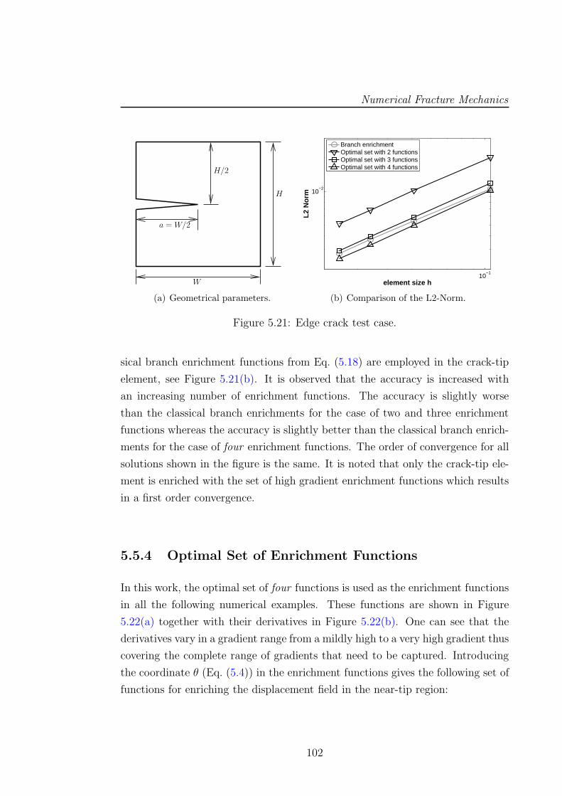
Numerical Fracture Mechanics
W
H
a = W/2
H/2
(a) Geometrical parameters.
10−1
10−2
element size h
L2 N
orm
Branch enrichmentOptimal set with 2 functionsOptimal set with 3 functionsOptimal set with 4 functions
(b) Comparison of the L2-Norm.
Figure 5.21: Edge crack test case.
sical branch enrichment functions from Eq. (5.18) are employed in the crack-tip
element, see Figure 5.21(b). It is observed that the accuracy is increased with
an increasing number of enrichment functions. The accuracy is slightly worse
than the classical branch enrichments for the case of two and three enrichment
functions whereas the accuracy is slightly better than the classical branch enrich-
ments for the case of four enrichment functions. The order of convergence for all
solutions shown in the figure is the same. It is noted that only the crack-tip ele-
ment is enriched with the set of high gradient enrichment functions which results
in a first order convergence.
5.5.4 Optimal Set of Enrichment Functions
In this work, the optimal set of four functions is used as the enrichment functions
in all the following numerical examples. These functions are shown in Figure
5.22(a) together with their derivatives in Figure 5.22(b). One can see that the
derivatives vary in a gradient range from a mildly high to a very high gradient thus
covering the complete range of gradients that need to be captured. Introducing
the coordinate θ (Eq. (5.4)) in the enrichment functions gives the following set of
functions for enriching the displacement field in the near-tip region:
102
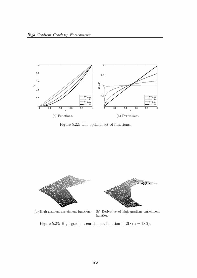
High-Gradient Crack-tip Enrichments
0 0.2 0.4 0.6 0.8 10
0.2
0.4
0.6
0.8
1
r
G
r = 1.02r = 1.20r = 1.57r = 1.95
(a) Functions.
0 0.2 0.4 0.6 0.8 10
0.5
1
1.5
2
r
dG/d
r
r = 1.02r = 1.20r = 1.57r = 1.95
(b) Derivatives.
Figure 5.22: The optimal set of functions.
(a) High gradient enrichment function. (b) Derivative of high gradient enrichmentfunction.
Figure 5.23: High gradient enrichment function in 2D (α = 1.02).
103
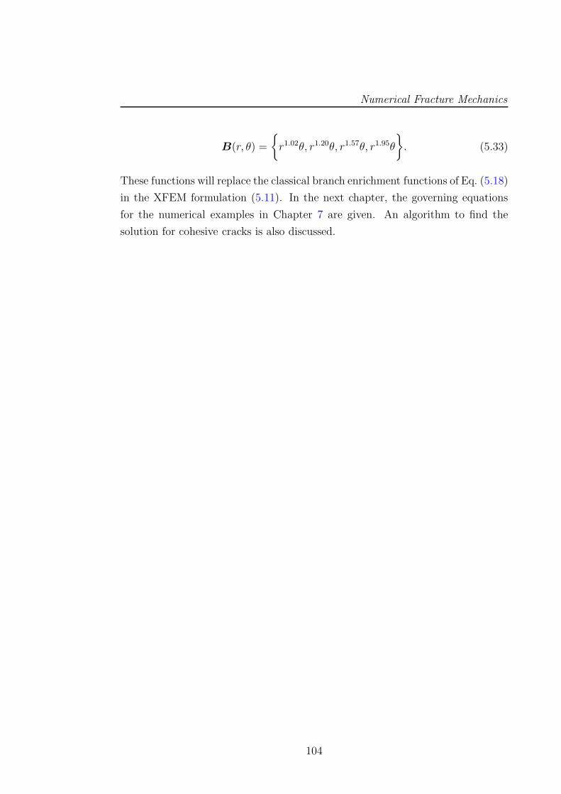
Numerical Fracture Mechanics
B(r, θ) =
r1.02θ, r1.20θ, r1.57θ, r1.95θ
. (5.33)
These functions will replace the classical branch enrichment functions of Eq. (5.18)
in the XFEM formulation (5.11). In the next chapter, the governing equations
for the numerical examples in Chapter 7 are given. An algorithm to find the
solution for cohesive cracks is also discussed.
104
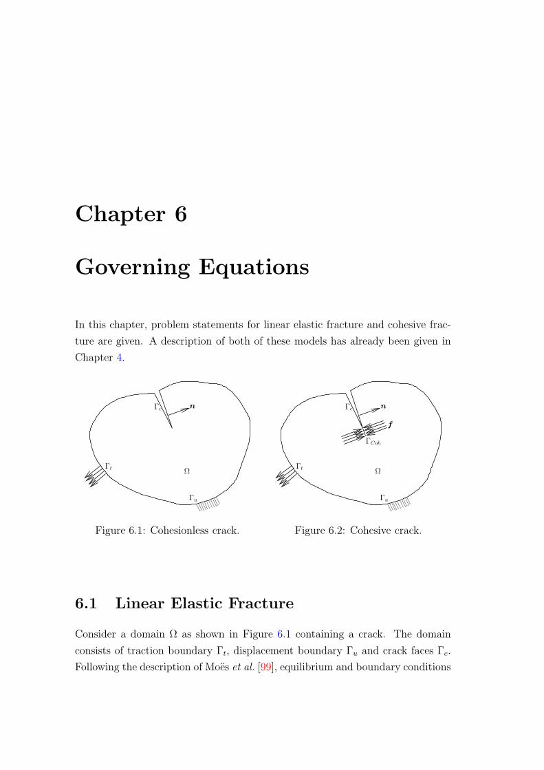
Chapter 6
Governing Equations
In this chapter, problem statements for linear elastic fracture and cohesive frac-
ture are given. A description of both of these models has already been given in
Chapter 4.
Γu
nΓc
Γt Ω
Figure 6.1: Cohesionless crack.
Γu
nΓc
ΓCoh
Γt Ω
f
Figure 6.2: Cohesive crack.
6.1 Linear Elastic Fracture
Consider a domain Ω as shown in Figure 6.1 containing a crack. The domain
consists of traction boundary Γt, displacement boundary Γu and crack faces Γc.
Following the description of Moes et al. [99], equilibrium and boundary conditions
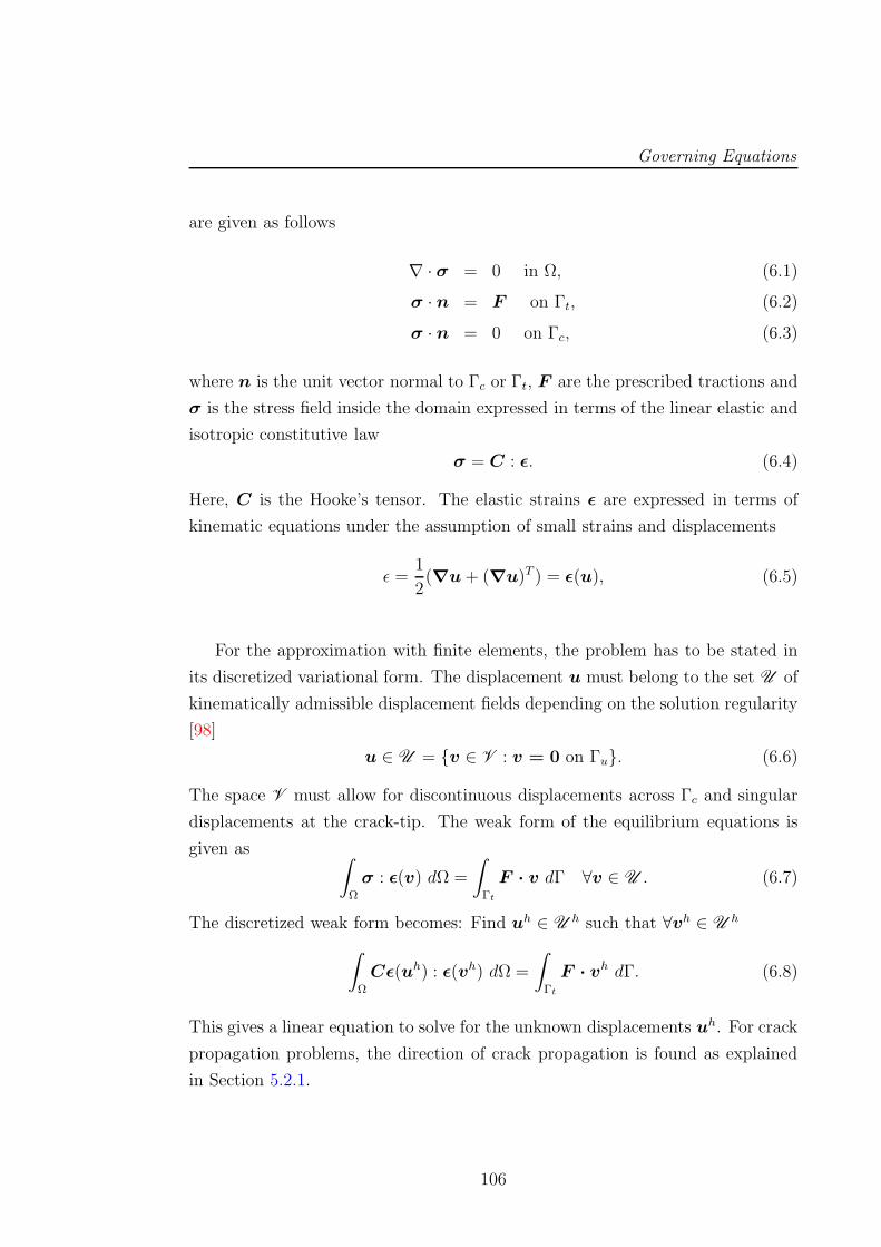
Governing Equations
are given as follows
∇ · σ = 0 in Ω, (6.1)
σ · n = F on Γt, (6.2)
σ · n = 0 on Γc, (6.3)
where n is the unit vector normal to Γc or Γt, F are the prescribed tractions and
σ is the stress field inside the domain expressed in terms of the linear elastic and
isotropic constitutive law
σ = C : ǫ. (6.4)
Here, C is the Hooke’s tensor. The elastic strains ǫ are expressed in terms of
kinematic equations under the assumption of small strains and displacements
ǫ =1
2(∇u+ (∇u)T ) = ǫ(u), (6.5)
For the approximation with finite elements, the problem has to be stated in
its discretized variational form. The displacement u must belong to the set U of
kinematically admissible displacement fields depending on the solution regularity
[98]
u ∈ U = v ∈ V : v = 0 on Γu. (6.6)
The space V must allow for discontinuous displacements across Γc and singular
displacements at the crack-tip. The weak form of the equilibrium equations is
given as ∫
Ω
σ : ǫ(v) dΩ =
∫
Γt
F · v dΓ ∀v ∈ U . (6.7)
The discretized weak form becomes: Find uh ∈ U h such that ∀vh ∈ U h
∫
Ω
Cǫ(uh) : ǫ(vh) dΩ =
∫
Γt
F · vh dΓ. (6.8)
This gives a linear equation to solve for the unknown displacements uh. For crack
propagation problems, the direction of crack propagation is found as explained
in Section 5.2.1.
106
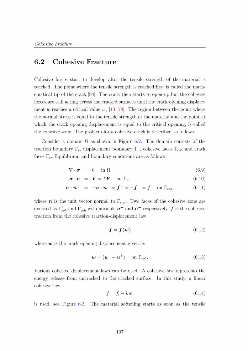
Cohesive Fracture
6.2 Cohesive Fracture
Cohesive forces start to develop after the tensile strength of the material is
reached. The point where the tensile strength is reached first is called the math-
ematical tip of the crack [98]. The crack then starts to open up but the cohesive
forces are still acting across the cracked surfaces until the crack opening displace-
ment w reaches a critical value wc [13, 78]. The region between the point where
the normal stress is equal to the tensile strength of the material and the point at
which the crack opening displacement is equal to the critical opening, is called
the cohesive zone. The problem for a cohesive crack is described as follows.
Consider a domain Ω as shown in Figure 6.2. The domain consists of the
traction boundary Γt, displacement boundary Γu, cohesive faces Γcoh and crack
faces Γc. Equilibrium and boundary conditions are as follows
∇ · σ = 0 in Ω, (6.9)
σ · n = F = λF on Γt, (6.10)
σ · n+ = −σ · n− = f+ = −f− = f on Γcoh, (6.11)
where n is the unit vector normal to Γcoh. Two faces of the cohesive zone are
denoted as Γ+coh and Γ−
coh with normals n+ and n− respectively, f is the cohesive
traction from the cohesive traction-displacement law
f = f(w) (6.12)
where w is the crack opening displacement given as
w = (u− − u+) on Γcoh. (6.13)
Various cohesive displacement laws can be used. A cohesive law represents the
energy release from uncracked to the cracked surface. In this study, a linear
cohesive law
f = ft − kw, (6.14)
is used, see Figure 6.3. The material softening starts as soon as the tensile
107
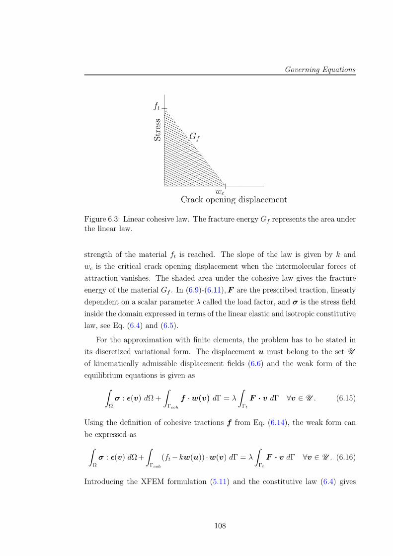
Governing Equations
ft
Str
ess
Crack opening displacementwc
Gf
Figure 6.3: Linear cohesive law. The fracture energy Gf represents the area underthe linear law.
strength of the material ft is reached. The slope of the law is given by k and
wc is the critical crack opening displacement when the intermolecular forces of
attraction vanishes. The shaded area under the cohesive law gives the fracture
energy of the material Gf . In (6.9)-(6.11),F are the prescribed traction, linearly
dependent on a scalar parameter λ called the load factor, and σ is the stress field
inside the domain expressed in terms of the linear elastic and isotropic constitutive
law, see Eq. (6.4) and (6.5).
For the approximation with finite elements, the problem has to be stated in
its discretized variational form. The displacement u must belong to the set U
of kinematically admissible displacement fields (6.6) and the weak form of the
equilibrium equations is given as
∫
Ω
σ : ǫ(v) dΩ+
∫
Γcoh
f ·w(v) dΓ = λ
∫
Γt
F · v dΓ ∀v ∈ U . (6.15)
Using the definition of cohesive tractions f from Eq. (6.14), the weak form can
be expressed as
∫
Ω
σ : ǫ(v) dΩ+
∫
Γcoh
(ft−kw(u)) ·w(v) dΓ = λ
∫
Γt
F · v dΓ ∀v ∈ U . (6.16)
Introducing the XFEM formulation (5.11) and the constitutive law (6.4) gives
108
Cohesive Fracture
the discretized weak form as: Find uh ∈ U h such that ∀vh ∈ U h
∫
Ω
Cǫ(uh) : ǫ(vh) dΩ+
∫
Γcoh
(ft− kw(uh)) ·w(vh) dΓ = λ
∫
Γt
F · vh dΓ. (6.17)
This is a non-linear equation which is to be solved for the unknown displacements
uh as well as the load factor λ.
The problem description for cohesive crack growth is completed as follows.
For a given crack path and the position of the mathematical tip, find the load
factor λ and displacements u such that the stress at the mathematical tip is equal
to the tensile strength ft. This condition is called the stress condition:
n · σ · n = ft. (6.18)
In the context of the XFEM, this approach is adopted by Zi and Belytschko [153].
The other approach that is used by Moes and Belytschko [98] is to find λ such
that the stress intensity factor (SIF) vanishes at the crack-tip
KI = 0. (6.19)
In the current study, the stress condition is used due to its intuitive nature and
ease of implementation. The displacement approximation (6.17) can be divided
into three parts
f int =
∫
Ω
ǫ(uh)Cǫ(vh) dΩ =
∫
Ω
BTCBdΩ · uh =K · uh, (6.20)
f coh =
∫
Γcoh
(ft − kw(uh)) ·w(vh) dΓ =
∫
Γcoh
f(w)NTndΓ, (6.21)
f ext = λ
∫
Γt
F · vh dΓ, (6.22)
109
Governing Equations
where B is the strain-displacement matrix given as
B =
D(x),x 0 0
0 D(x),y 0
0 0 D(x),z
D(x),y D(x),x 0
D(x),z 0 D(x),x
D(x),z D(x),y
, (6.23)
with D(x) is given as
D(x) =[
Ni(x) Mi(x)]
, (6.24)
where Ni(x) are the standard FE shape functions and Mi(x) are the local crack-
tip enrichment functions as given in Eq. (5.11)
Mi(x) = N⋆i (x) ·
[Ck(r, θ)−Ck(r, θi)
]. (6.25)
The algorithm given by Zi & Belytschko [153] is based on non-linear Newton-
Raphson iterations for the convergence of the displacements uh and the load factor
λ in order to satisfy both (6.17) and (6.18). The algorithm is given as follows. In
order to satisfy the stress condition of Eq. (6.18), an operator S = MT · C ·Bis defined to calculate the stress at the crack-tip as
S · uh = ft, (6.26)
where
M =[
n2x n2
y n2z nxny nxnz nynz
]′(6.27)
The residual of the Newton-Raphson method is given by
r =
[
K · uh − f extλ− f coh
ft − Suh
]
(6.28)
110
Cohesive Fracture
and the Jacobian is given by
J =
K − ∂f coh(uh)
∂u−f ext
−S 0
, (6.29)
where the derivative of the cohesive force is given as
∂f coh(uh)
∂u=
∫
Γcoh
∂f(w)
∂wNT · n · nT ·NdΓ (6.30)
The independent variables u and λ are updated in iteration i as
[
ui
λi
]
= −(J i−1)−1 · ri−1. (6.31)
The algorithm is given as
1. Construct the stiffness matrix K from Eq. (6.20).
2. Find the derivatives of the cohesive forces with respect to the nodal dis-
placements.
3. Compute the residual from Eq. (6.28) and the Jacobian from Eq. (6.29).
4. Find the increments from Eq. (6.31).
5. Iterate until u and λ converges.
In the case of 3D cohesive crack problems, a number of discrete points are
specified along the crack front. In the first iteration of the Newton Raphson loop,
the operator (6.26) is built for the point that is in the middle of the crack front.
In each subsequent iteration the operator (6.26) is built for the point having the
maximum stress. This procedure ensures the maximum normal stress along the
crack front to be bounded by ft from above. This algorithm is proposed here
for the first time and the results shown in Section 7.4 show the success of the
algorithm.
111
Governing Equations
112
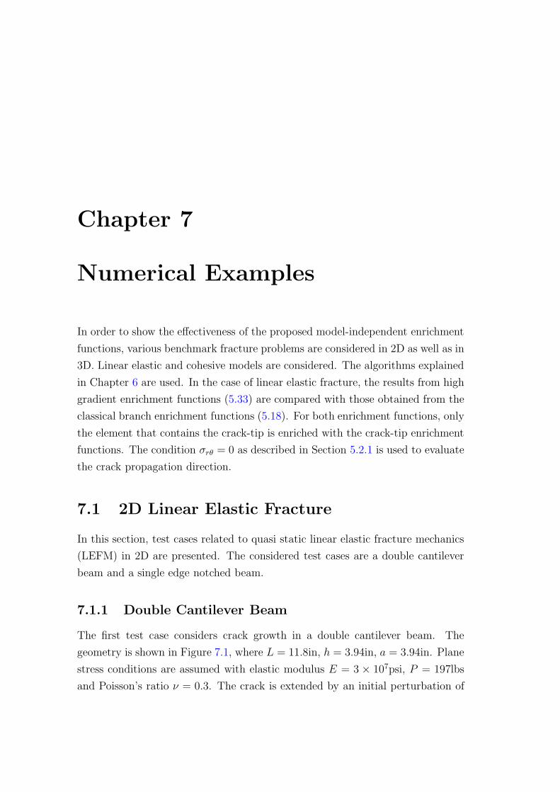
Chapter 7
Numerical Examples
In order to show the effectiveness of the proposed model-independent enrichment
functions, various benchmark fracture problems are considered in 2D as well as in
3D. Linear elastic and cohesive models are considered. The algorithms explained
in Chapter 6 are used. In the case of linear elastic fracture, the results from high
gradient enrichment functions (5.33) are compared with those obtained from the
classical branch enrichment functions (5.18). For both enrichment functions, only
the element that contains the crack-tip is enriched with the crack-tip enrichment
functions. The condition σrθ = 0 as described in Section 5.2.1 is used to evaluate
the crack propagation direction.
7.1 2D Linear Elastic Fracture
In this section, test cases related to quasi static linear elastic fracture mechanics
(LEFM) in 2D are presented. The considered test cases are a double cantilever
beam and a single edge notched beam.
7.1.1 Double Cantilever Beam
The first test case considers crack growth in a double cantilever beam. The
geometry is shown in Figure 7.1, where L = 11.8in, h = 3.94in, a = 3.94in. Plane
stress conditions are assumed with elastic modulus E = 3 × 10⁷psi, P = 197lbs
and Poisson’s ratio ν = 0.3. The crack is extended by an initial perturbation of
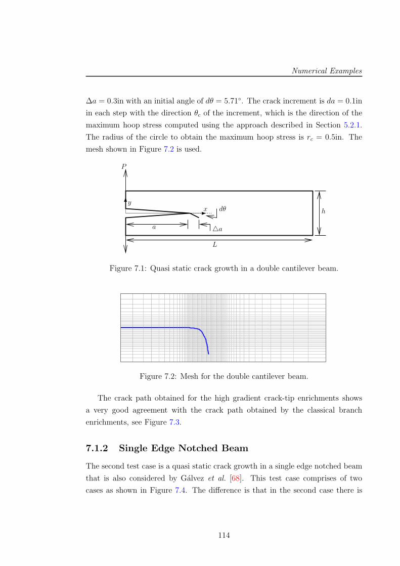
Numerical Examples
∆a = 0.3in with an initial angle of dθ = 5.71. The crack increment is da = 0.1in
in each step with the direction θc of the increment, which is the direction of the
maximum hoop stress computed using the approach described in Section 5.2.1.
The radius of the circle to obtain the maximum hoop stress is rc = 0.5in. The
mesh shown in Figure 7.2 is used.
y
a
dθ
L
h
P
a
x
Figure 7.1: Quasi static crack growth in a double cantilever beam.
Figure 7.2: Mesh for the double cantilever beam.
The crack path obtained for the high gradient crack-tip enrichments shows
a very good agreement with the crack path obtained by the classical branch
enrichments, see Figure 7.3.
7.1.2 Single Edge Notched Beam
The second test case is a quasi static crack growth in a single edge notched beam
that is also considered by Galvez et al. [68]. This test case comprises of two
cases as shown in Figure 7.4. The difference is that in the second case there is
114
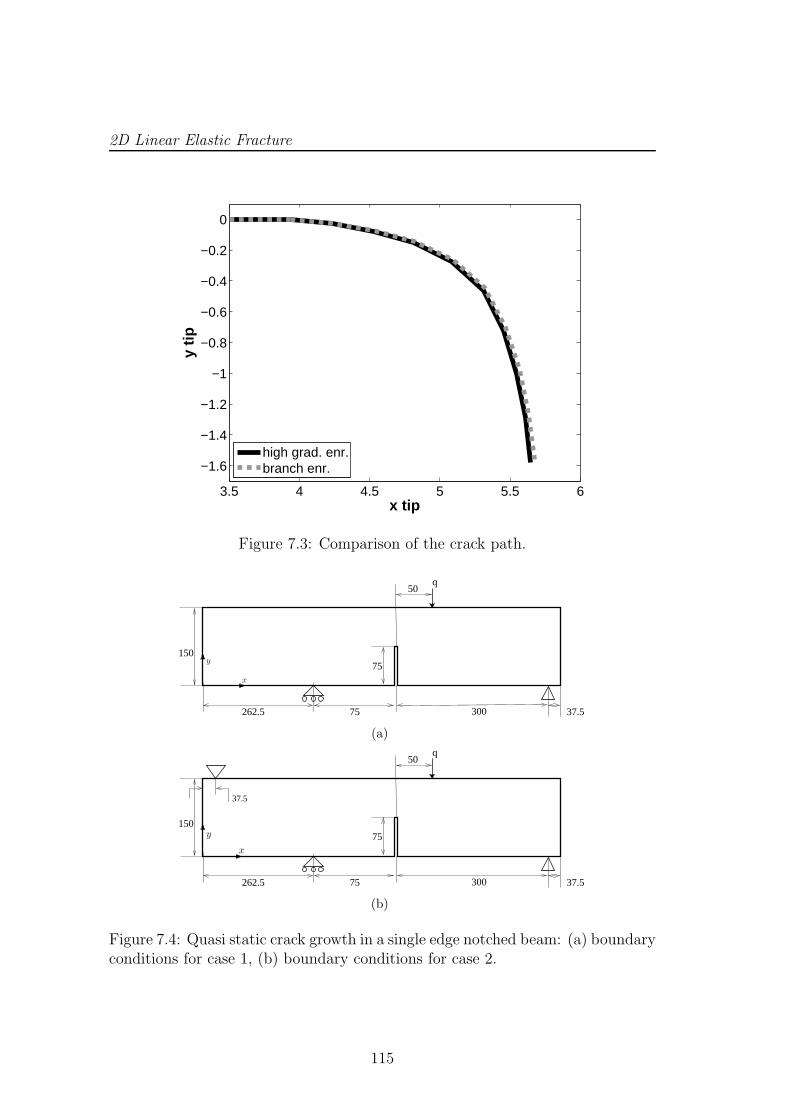
2D Linear Elastic Fracture
3.5 4 4.5 5 5.5 6
−1.6
−1.4
−1.2
−1
−0.8
−0.6
−0.4
−0.2
0
x tip
y tip
high grad. enr.branch enr.
Figure 7.3: Comparison of the crack path.
262.5 75
50
300
15075
q
37.5
y
x
(a)
262.5 75
50
300
15075
q
37.5
37.5
y
x
(b)
Figure 7.4: Quasi static crack growth in a single edge notched beam: (a) boundaryconditions for case 1, (b) boundary conditions for case 2.
115
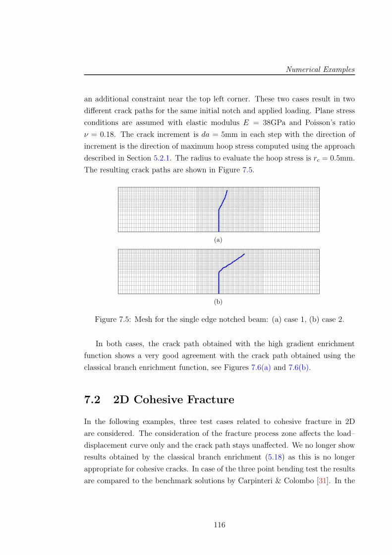
Numerical Examples
an additional constraint near the top left corner. These two cases result in two
different crack paths for the same initial notch and applied loading. Plane stress
conditions are assumed with elastic modulus E = 38GPa and Poisson’s ratio
ν = 0.18. The crack increment is da = 5mm in each step with the direction of
increment is the direction of maximum hoop stress computed using the approach
described in Section 5.2.1. The radius to evaluate the hoop stress is rc = 0.5mm.
The resulting crack paths are shown in Figure 7.5.
(a)
(b)
Figure 7.5: Mesh for the single edge notched beam: (a) case 1, (b) case 2.
In both cases, the crack path obtained with the high gradient enrichment
function shows a very good agreement with the crack path obtained using the
classical branch enrichment function, see Figures 7.6(a) and 7.6(b).
7.2 2D Cohesive Fracture
In the following examples, three test cases related to cohesive fracture in 2D
are considered. The consideration of the fracture process zone affects the load–
displacement curve only and the crack path stays unaffected. We no longer show
results obtained by the classical branch enrichment (5.18) as this is no longer
appropriate for cohesive cracks. In case of the three point bending test the results
are compared to the benchmark solutions by Carpinteri & Colombo [31]. In the
116
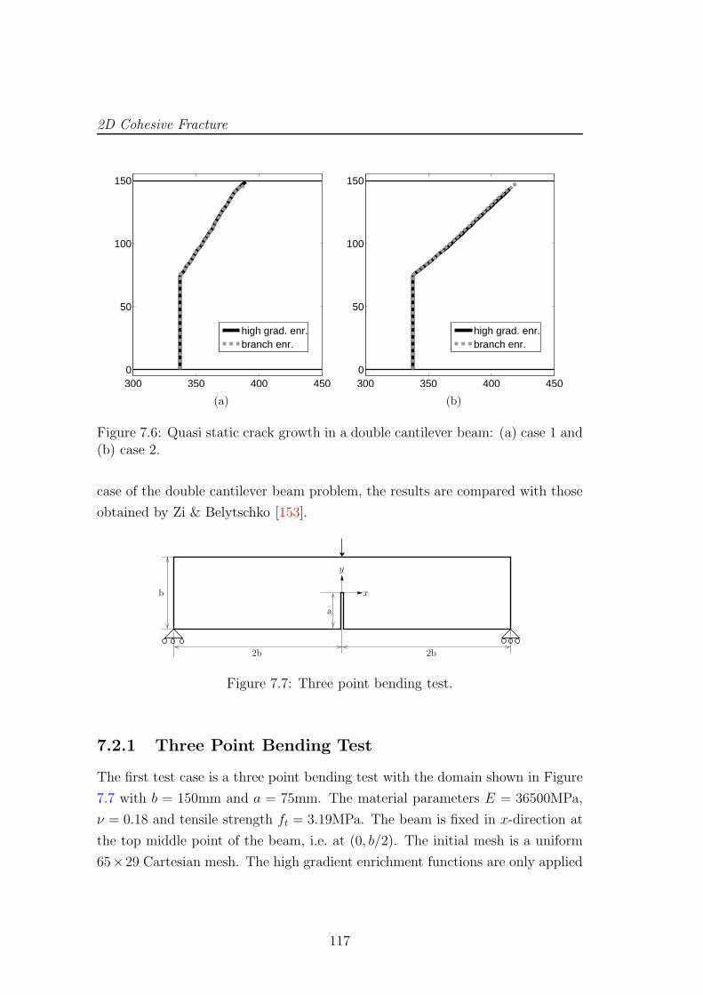
2D Cohesive Fracture
300 350 400 4500
50
100
150
high grad. enr.branch enr.
(a)
300 350 400 4500
50
100
150
high grad. enr.branch enr.
(b)
Figure 7.6: Quasi static crack growth in a double cantilever beam: (a) case 1 and(b) case 2.
case of the double cantilever beam problem, the results are compared with those
obtained by Zi & Belytschko [153].
y
2b 2b
b
a
x
Figure 7.7: Three point bending test.
7.2.1 Three Point Bending Test
The first test case is a three point bending test with the domain shown in Figure
7.7 with b = 150mm and a = 75mm. The material parameters E = 36500MPa,
ν = 0.18 and tensile strength ft = 3.19MPa. The beam is fixed in x-direction at
the top middle point of the beam, i.e. at (0, b/2). The initial mesh is a uniform
65×29 Cartesian mesh. The high gradient enrichment functions are only applied
117
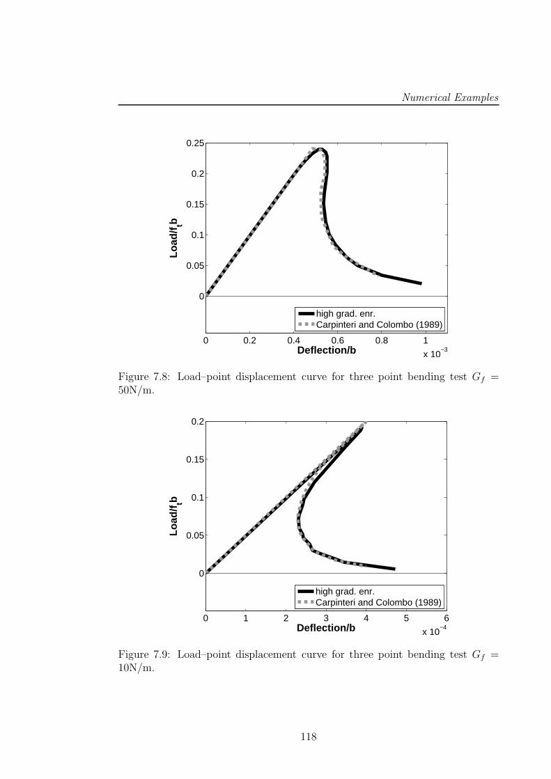
Numerical Examples
0 0.2 0.4 0.6 0.8 1
x 10−3
0
0.05
0.1
0.15
0.2
0.25
Deflection/b
Load
/ftb
high grad. enr.Carpinteri and Colombo (1989)
Figure 7.8: Load–point displacement curve for three point bending test Gf =50N/m.
0 1 2 3 4 5 6
x 10−4
0
0.05
0.1
0.15
0.2
Deflection/b
Load
/ftb
high grad. enr.Carpinteri and Colombo (1989)
Figure 7.9: Load–point displacement curve for three point bending test Gf =10N/m.
118
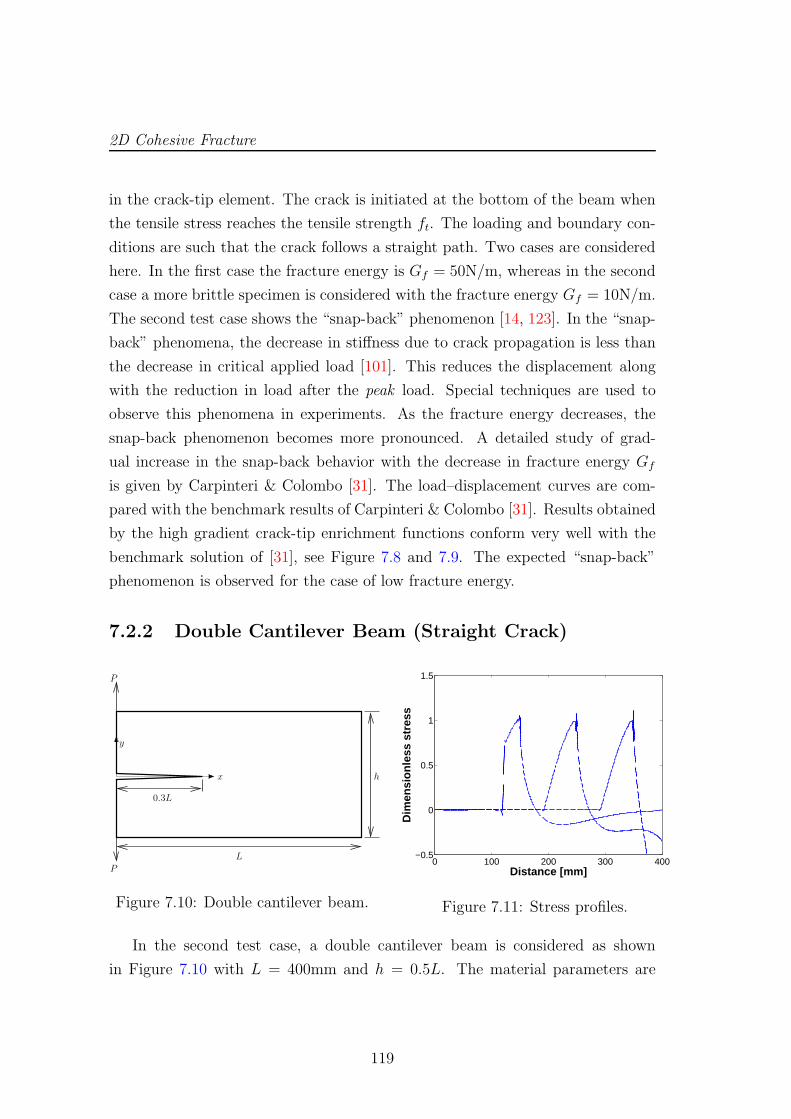
2D Cohesive Fracture
in the crack-tip element. The crack is initiated at the bottom of the beam when
the tensile stress reaches the tensile strength ft. The loading and boundary con-
ditions are such that the crack follows a straight path. Two cases are considered
here. In the first case the fracture energy is Gf = 50N/m, whereas in the second
case a more brittle specimen is considered with the fracture energy Gf = 10N/m.
The second test case shows the “snap-back” phenomenon [14, 123]. In the “snap-
back” phenomena, the decrease in stiffness due to crack propagation is less than
the decrease in critical applied load [101]. This reduces the displacement along
with the reduction in load after the peak load. Special techniques are used to
observe this phenomena in experiments. As the fracture energy decreases, the
snap-back phenomenon becomes more pronounced. A detailed study of grad-
ual increase in the snap-back behavior with the decrease in fracture energy Gf
is given by Carpinteri & Colombo [31]. The load–displacement curves are com-
pared with the benchmark results of Carpinteri & Colombo [31]. Results obtained
by the high gradient crack-tip enrichment functions conform very well with the
benchmark solution of [31], see Figure 7.8 and 7.9. The expected “snap-back”
phenomenon is observed for the case of low fracture energy.
7.2.2 Double Cantilever Beam (Straight Crack)
y
P
P
0.3L
L
hx
Figure 7.10: Double cantilever beam.
0 100 200 300 400−0.5
0
0.5
1
1.5
Distance [mm]
Dim
ensi
onle
ss s
tres
s
Figure 7.11: Stress profiles.
In the second test case, a double cantilever beam is considered as shown
in Figure 7.10 with L = 400mm and h = 0.5L. The material parameters are
119
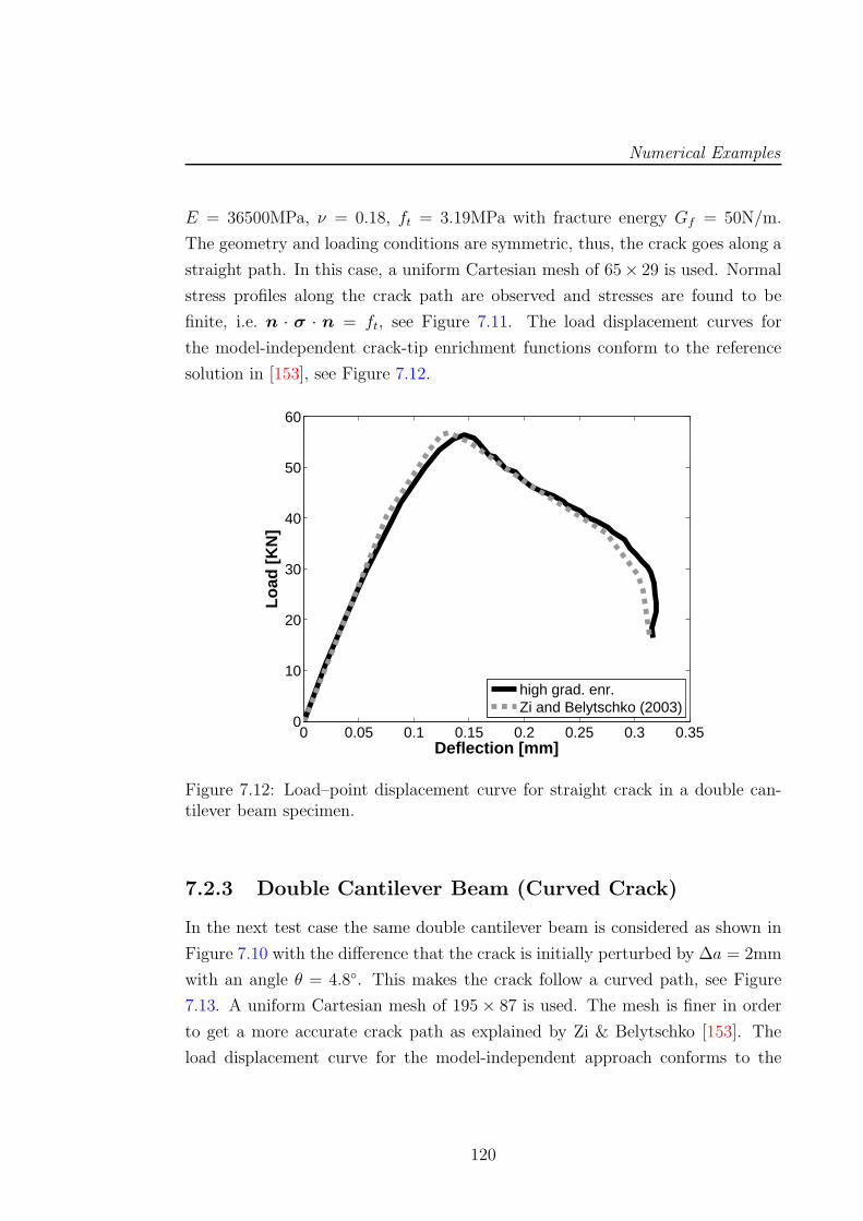
Numerical Examples
E = 36500MPa, ν = 0.18, ft = 3.19MPa with fracture energy Gf = 50N/m.
The geometry and loading conditions are symmetric, thus, the crack goes along a
straight path. In this case, a uniform Cartesian mesh of 65× 29 is used. Normal
stress profiles along the crack path are observed and stresses are found to be
finite, i.e. n · σ · n = ft, see Figure 7.11. The load displacement curves for
the model-independent crack-tip enrichment functions conform to the reference
solution in [153], see Figure 7.12.
0 0.05 0.1 0.15 0.2 0.25 0.3 0.350
10
20
30
40
50
60
Deflection [mm]
Load
[KN
]
high grad. enr.Zi and Belytschko (2003)
Figure 7.12: Load–point displacement curve for straight crack in a double can-tilever beam specimen.
7.2.3 Double Cantilever Beam (Curved Crack)
In the next test case the same double cantilever beam is considered as shown in
Figure 7.10 with the difference that the crack is initially perturbed by ∆a = 2mm
with an angle θ = 4.8. This makes the crack follow a curved path, see Figure
7.13. A uniform Cartesian mesh of 195 × 87 is used. The mesh is finer in order
to get a more accurate crack path as explained by Zi & Belytschko [153]. The
load displacement curve for the model-independent approach conforms to the
120
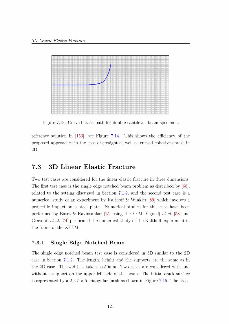
3D Linear Elastic Fracture
Figure 7.13: Curved crack path for double cantilever beam specimen.
reference solution in [153], see Figure 7.14. This shows the efficiency of the
proposed approaches in the case of straight as well as curved cohesive cracks in
2D.
7.3 3D Linear Elastic Fracture
Two test cases are considered for the linear elastic fracture in three dimensions.
The first test case is the single edge notched beam problem as described by [68],
related to the setting discussed in Section 7.1.2, and the second test case is a
numerical study of an experiment by Kalthoff & Winkler [89] which involves a
projectile impact on a steel plate. Numerical studies for this case have been
performed by Batra & Ravinsankar [15] using the FEM. Elguedj et al. [58] and
Gravouil et al. [74] performed the numerical study of the Kalthoff experiment in
the frame of the XFEM.
7.3.1 Single Edge Notched Beam
The single edge notched beam test case is considered in 3D similar to the 2D
case in Section 7.1.2. The length, height and the supports are the same as in
the 2D case. The width is taken as 50mm. Two cases are considered with and
without a support on the upper left side of the beam. The initial crack surface
is represented by a 2× 5× 5 triangular mesh as shown in Figure 7.15. The crack
121
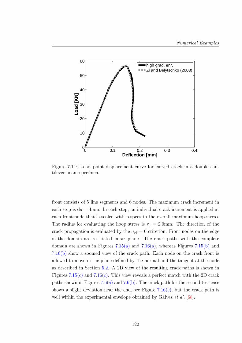
Numerical Examples
0 0.1 0.2 0.3 0.40
10
20
30
40
50
60
Deflection [mm]
Load
[KN
]
high grad. enr.Zi and Belytschko (2003)
Figure 7.14: Load–point displacement curve for curved crack in a double can-tilever beam specimen.
front consists of 5 line segments and 6 nodes. The maximum crack increment in
each step is da = 4mm. In each step, an individual crack increment is applied at
each front node that is scaled with respect to the overall maximum hoop stress.
The radius for evaluating the hoop stress is rc = 2.0mm. The direction of the
crack propagation is evaluated by the σrθ = 0 criterion. Front nodes on the edge
of the domain are restricted in xz plane. The crack paths with the complete
domain are shown in Figures 7.15(a) and 7.16(a), whereas Figures 7.15(b) and
7.16(b) show a zoomed view of the crack path. Each node on the crack front is
allowed to move in the plane defined by the normal and the tangent at the node
as described in Section 5.2. A 2D view of the resulting crack paths is shown in
Figures 7.15(c) and 7.16(c). This view reveals a perfect match with the 2D crack
paths shown in Figures 7.6(a) and 7.6(b). The crack path for the second test case
shows a slight deviation near the end, see Figure 7.16(c), but the crack path is
well within the experimental envelope obtained by Galvez et al. [68].
122
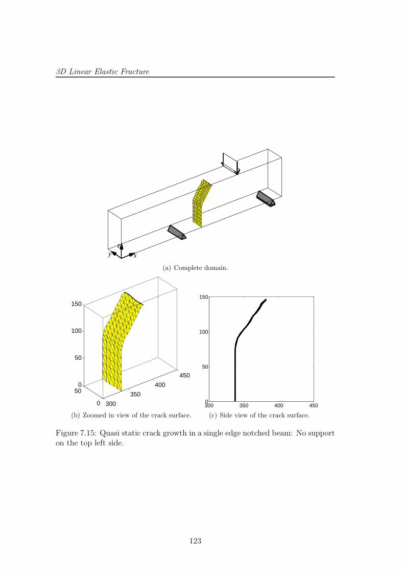
3D Linear Elastic Fracture
x
zy
(a) Complete domain.
300
350
400
450
0
500
50
100
150
(b) Zoomed in view of the crack surface.
300 350 400 4500
50
100
150
(c) Side view of the crack surface.
Figure 7.15: Quasi static crack growth in a single edge notched beam: No supporton the top left side.
123
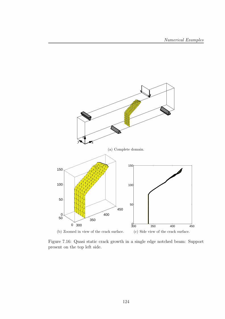
Numerical Examples
x
zy
(a) Complete domain.
300
350
400
450
0
500
50
100
150
(b) Zoomed in view of the crack surface.
300 350 400 4500
50
100
150
(c) Side view of the crack surface.
Figure 7.16: Quasi static crack growth in a single edge notched beam: Supportpresent on the top left side.
124
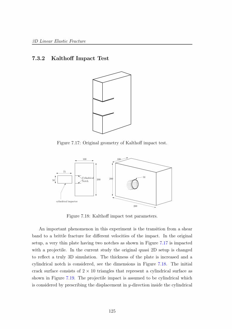
3D Linear Elastic Fracture
7.3.2 Kalthoff Impact Test
Figure 7.17: Original geometry of Kalthoff impact test.
Notch
75
50
cylindrical impactor
100
20050
200
200
100
Cylindrical
Figure 7.18: Kalthoff impact test parameters.
An important phenomenon in this experiment is the transition from a shear
band to a brittle fracture for different velocities of the impact. In the original
setup, a very thin plate having two notches as shown in Figure 7.17 is impacted
with a projectile. In the current study the original quasi 2D setup is changed
to reflect a truly 3D simulation. The thickness of the plate is increased and a
cylindrical notch is considered, see the dimensions in Figure 7.18. The initial
crack surface consists of 2 × 10 triangles that represent a cylindrical surface as
shown in Figure 7.19. The projectile impact is assumed to be cylindrical which
is considered by prescribing the displacement in y-direction inside the cylindrical
125
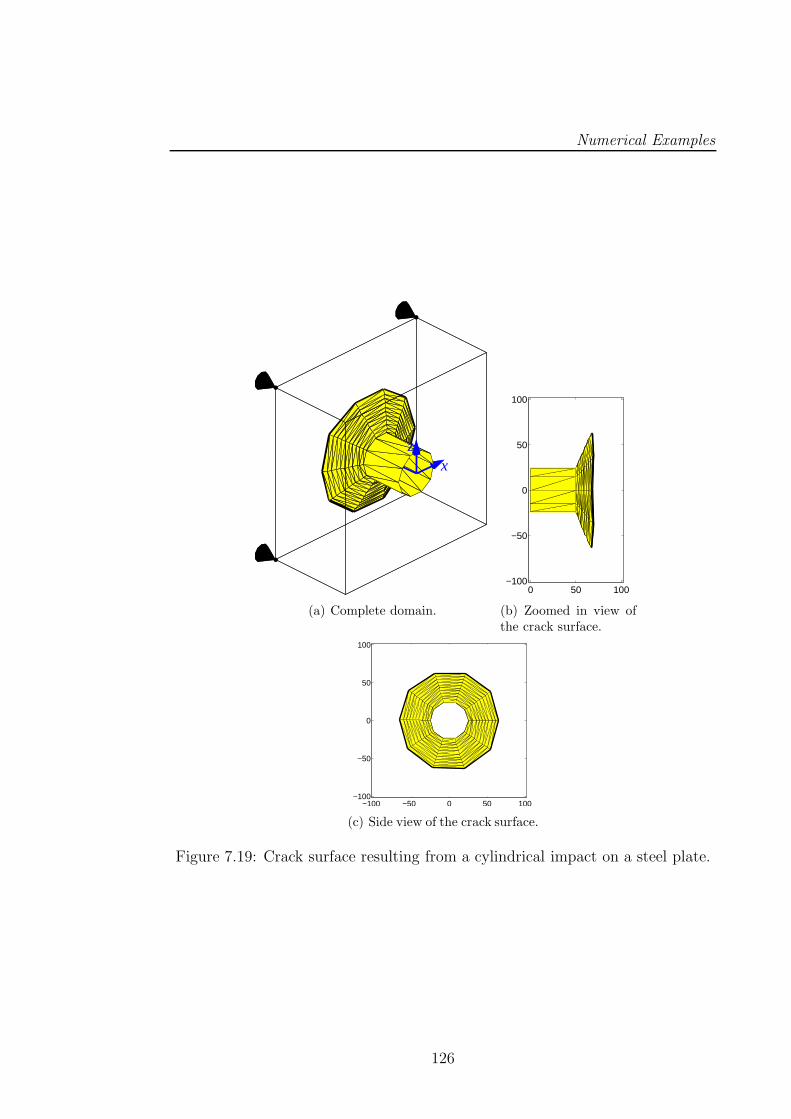
Numerical Examples
y xz
(a) Complete domain.
0 50 100−100
−50
0
50
100
(b) Zoomed in view ofthe crack surface.
−100 −50 0 50 100−100
−50
0
50
100
(c) Side view of the crack surface.
Figure 7.19: Crack surface resulting from a cylindrical impact on a steel plate.
126
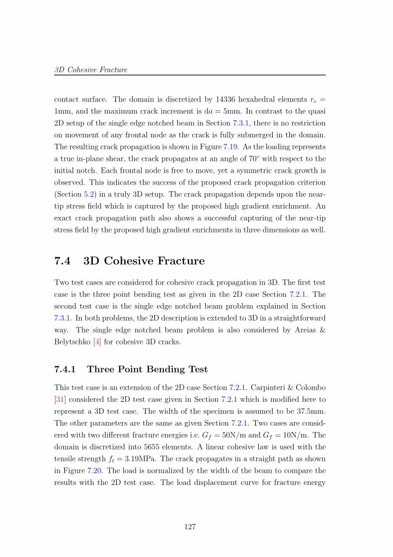
3D Cohesive Fracture
contact surface. The domain is discretized by 14336 hexahedral elements rc =
1mm, and the maximum crack increment is da = 5mm. In contrast to the quasi
2D setup of the single edge notched beam in Section 7.3.1, there is no restriction
on movement of any frontal node as the crack is fully submerged in the domain.
The resulting crack propagation is shown in Figure 7.19. As the loading represents
a true in-plane shear, the crack propagates at an angle of 70 with respect to the
initial notch. Each frontal node is free to move, yet a symmetric crack growth is
observed. This indicates the success of the proposed crack propagation criterion
(Section 5.2) in a truly 3D setup. The crack propagation depends upon the near-
tip stress field which is captured by the proposed high gradient enrichment. An
exact crack propagation path also shows a successful capturing of the near-tip
stress field by the proposed high gradient enrichments in three dimensions as well.
7.4 3D Cohesive Fracture
Two test cases are considered for cohesive crack propagation in 3D. The first test
case is the three point bending test as given in the 2D case Section 7.2.1. The
second test case is the single edge notched beam problem explained in Section
7.3.1. In both problems, the 2D description is extended to 3D in a straightforward
way. The single edge notched beam problem is also considered by Areias &
Belytschko [4] for cohesive 3D cracks.
7.4.1 Three Point Bending Test
This test case is an extension of the 2D case Section 7.2.1. Carpinteri & Colombo
[31] considered the 2D test case given in Section 7.2.1 which is modified here to
represent a 3D test case. The width of the specimen is assumed to be 37.5mm.
The other parameters are the same as given Section 7.2.1. Two cases are consid-
ered with two different fracture energies i.e. Gf = 50N/m and Gf = 10N/m. The
domain is discretized into 5655 elements. A linear cohesive law is used with the
tensile strength ft = 3.19MPa. The crack propagates in a straight path as shown
in Figure 7.20. The load is normalized by the width of the beam to compare the
results with the 2D test case. The load displacement curve for fracture energy
127
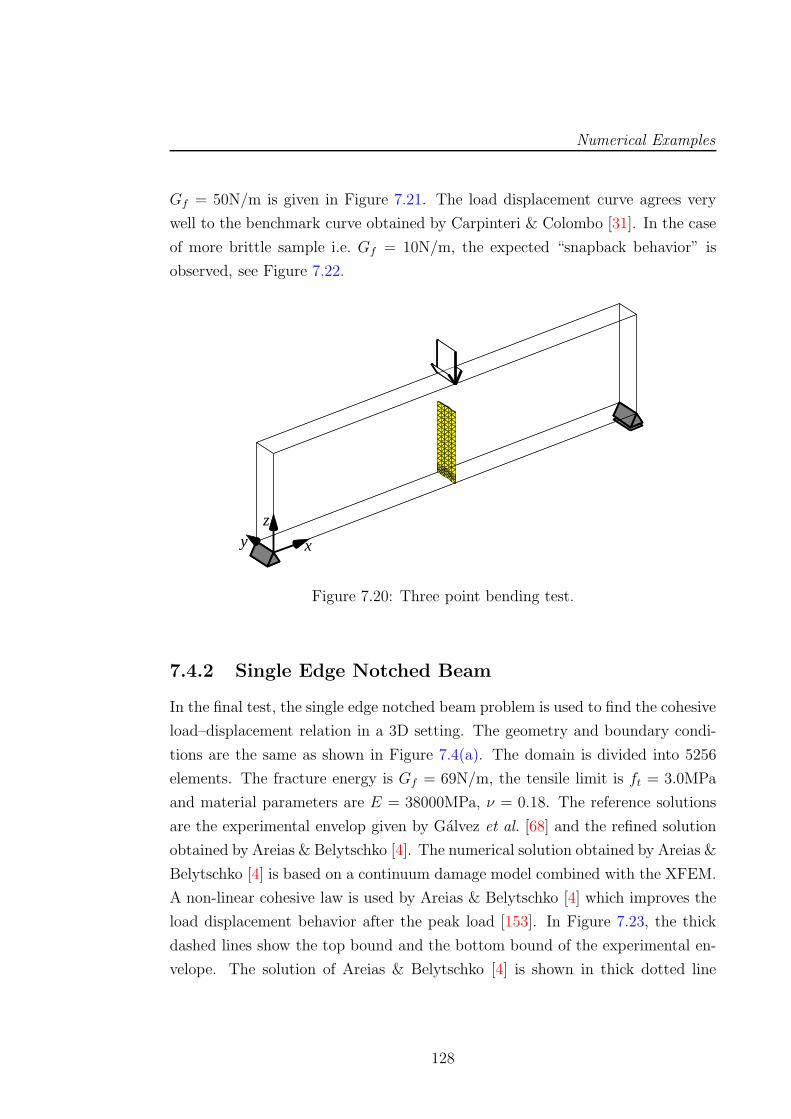
Numerical Examples
Gf = 50N/m is given in Figure 7.21. The load displacement curve agrees very
well to the benchmark curve obtained by Carpinteri & Colombo [31]. In the case
of more brittle sample i.e. Gf = 10N/m, the expected “snapback behavior” is
observed, see Figure 7.22.
x
zy
Figure 7.20: Three point bending test.
7.4.2 Single Edge Notched Beam
In the final test, the single edge notched beam problem is used to find the cohesive
load–displacement relation in a 3D setting. The geometry and boundary condi-
tions are the same as shown in Figure 7.4(a). The domain is divided into 5256
elements. The fracture energy is Gf = 69N/m, the tensile limit is ft = 3.0MPa
and material parameters are E = 38000MPa, ν = 0.18. The reference solutions
are the experimental envelop given by Galvez et al. [68] and the refined solution
obtained by Areias & Belytschko [4]. The numerical solution obtained by Areias &
Belytschko [4] is based on a continuum damage model combined with the XFEM.
A non-linear cohesive law is used by Areias & Belytschko [4] which improves the
load displacement behavior after the peak load [153]. In Figure 7.23, the thick
dashed lines show the top bound and the bottom bound of the experimental en-
velope. The solution of Areias & Belytschko [4] is shown in thick dotted line
128
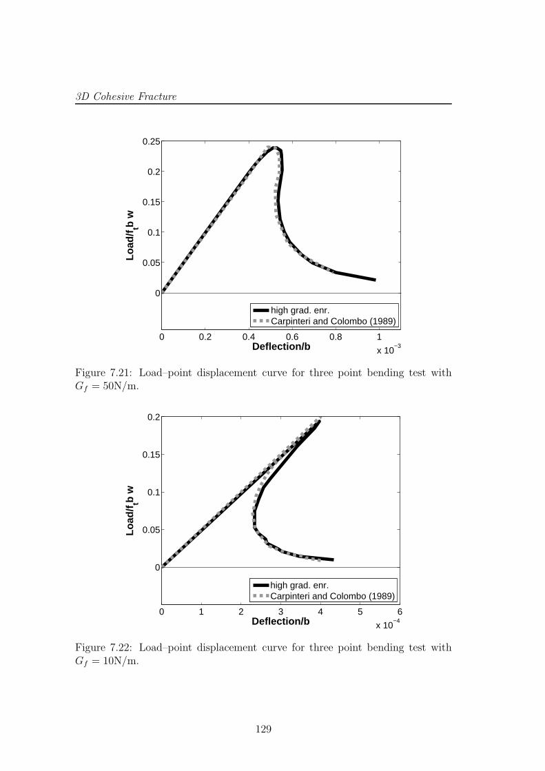
3D Cohesive Fracture
0 0.2 0.4 0.6 0.8 1
x 10−3
0
0.05
0.1
0.15
0.2
0.25
Deflection/b
Load
/ftb
w
high grad. enr.Carpinteri and Colombo (1989)
Figure 7.21: Load–point displacement curve for three point bending test withGf = 50N/m.
0 1 2 3 4 5 6
x 10−4
0
0.05
0.1
0.15
0.2
Deflection/b
Load
/ftb
w
high grad. enr.Carpinteri and Colombo (1989)
Figure 7.22: Load–point displacement curve for three point bending test withGf = 10N/m.
129
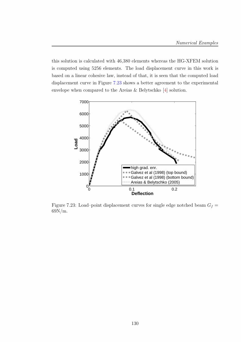
Numerical Examples
this solution is calculated with 46,380 elements whereas the HG-XFEM solution
is computed using 5256 elements. The load displacement curve in this work is
based on a linear cohesive law, instead of that, it is seen that the computed load
displacement curve in Figure 7.23 shows a better agreement to the experimental
envelope when compared to the Areias & Belytschko [4] solution.
0 0.1 0.20
1000
2000
3000
4000
5000
6000
7000
Deflection
Load
high grad. enr.Galvez et al (1998) (top bound)Galvez et al (1998) (bottom bound)Areias & Belytschko (2005)
Figure 7.23: Load–point displacement curves for single edge notched beam Gf =69N/m.
130
Chapter 8
Conclusions and Outlook
8.1 Conclusions
In this study, a new enrichment methodology in the XFEM has been developed
in order to capture arbitrary high gradient solutions. High gradient enrichment
functions are developed based on the type of high gradient. A suitable function is
first selected that can be scaled to capture any gradient of that type. A systematic
study which involves an optimization procedure is performed in order to find the
best set of enrichment functions for a particular number of enrichments. This set
of enrichment functions can capture a high gradient solution irrespective of the
steepness of the gradient.
The method is successfully applied to 1D and 2D convection dominated prob-
lems in order to investigate general properties of the HG-XFEM and to capture
arbitrary high gradients across close interfaces. The model problems consid-
ered to simulate convection dominated phenomena includes the nonlinear Burgers
equation and the linear advection-diffusion equation. For temporal discretization
a time-stepping scheme is used for the case of stationary high gradients whereas
the space-time discretization with discontinuous Galerkin in time is used for mov-
ing high gradients. The test cases considered in one and two-dimensions show a
high quality resolution of arbitrary high gradients across close interfaces without
mesh manipulation and stabilization.
After the successful application of the HG-XFEM to the convection domi-
nated problems, the focus is shifted to fracture mechanics. We are interested in
Conclusions and Outlook
the propagation of cracks which depends upon the crack-tip stress field. In the
XFEM, the crack-tip stress field is captured by the crack-tip enrichment func-
tions. These functions are not easy to design and they require the knowledge
of the asymptotic near-tip fields. In this work, a set of high gradient crack-tip
enrichment functions is designed in order to capture the crack-tip stress field in a
model independent fashion without knowing the exact crack-tip stress behavior.
In order to confirm the model independence, the new set of enrichment functions
is applied to problems in linear elastic as well as cohesive fracture. For an accu-
rate crack representation and efficient crack update, the hybrid explicit-implicit
crack representation by Fries & Baydoun [65] is used. This approach involves a
combination of explicit crack representation and implicit level-set functions. The
implicit level-set functions are advantageous for the XFEM in order to determine
where and how to enrich. It is also useful in subdividing the elements for in-
tegration purposes. The explicit representation of cracks by a polygon in two
dimensions and by a polyhedron in three dimensions is useful in representing a
non-smooth crack path and driving the crack extension. A useful combination of
both the explicit and the implicit representation makes it possible to treat the
two and three-dimensional crack simulation in a consistent manner.
Two and three-dimensional test cases are considered for straight and curved
crack propagation. Linear elastic and cohesive fracture models are considered.
In the case of cohesive fracture, the algorithm proposed by Zi & Belytschko
[153] is used. In this algorithm, the non-linear constitutive equations are solved
using Newton-Raphson iterations. The algorithm is adapted for applications
in three dimensions, where the maximum normal stress along the crack front is
bound from above by the yield stress of the material. Computational results show
very good agreement with available experimental data or established benchmark
computational results. Thus the overall objective of developing an enrichment
scheme to capture arbitrary high gradients near the tip of an open interface has
been achieved.
132
Outlook
8.2 Outlook
After the success of the HG-XFEM in the case of two and three dimensional frac-
tures involving linear elastic and cohesive models, the HG-XFEM can be applied
to more complex fracture situations. Multiple cracks can be considered to sim-
ulate crack interaction. Test cases from practical industrial applications can be
considered involving complex three dimensional mixed mode fractures. Cracks
involving other nonlinear materials such as elasto-plastic or visco-elastic materials
might be considered to make profit of the model independence of high gradient
enrichment functions. Cracks involving physical nonlinearities such as cracks in
composite materials or cracks across material interfaces pose challenging applica-
tion for the HG-XFEM. In addition to material and physical nonlinearities, cracks
involving geometric nonlinearities and dynamic cracks can also be considered.
It is important to note that this procedure of capturing high gradient so-
lutions with enrichment functions is not limited to fracture mechanics. Future
applications can come from a great variety of fields. The enrichment procedure
can be applied to most of the situations where mesh refinement would be needed
otherwise. Possible fields of applications include but are not limited to phase
transition and solidification problems and resolving shear bands. High gradients
developing due convection dominated phenomena, for example, in welding sim-
ulation is another prospective application of the HG-XFEM. Thus the objective
of this work has been achieved with a large scope of extensions to various fields
of applications.
133

Conclusions and Outlook
134
References
[1] Abbas, S. & Fries, T.P. (2010). A unified enrichment scheme for fracture
problems. In IOP Conf. Ser.: Mater. Sci. Eng.10 012045 . 5, 98
[2] Abbas, S., Alizada, A. & Fries, T.P. (2010). The XFEM for high-
gradient solutions in convection-dominated problems. Internat. J. Numer.
Methods Engrg., 82, 1044–1072. 6, 13, 26
[3] Anderson, T.L. (2005). FRACTURE MECHANICS Fundamentals and
Applications . Taylor & Francis, 3rd edn. xii, 2, 49, 58, 66
[4] Areias, P. & Belytschko, T. (2005). Analysis of three-dimensional
crack initiation and propagation using the extended finite element method.
Internat. J. Numer. Methods Engrg., 63, 760 – 788. 127, 128, 130
[5] Areias, P. & Belytschko, T. (2006). Two-scale shear band evolution
by local partition of unity. Internat. J. Numer. Methods Engrg., 66, 878 –
910. 12
[6] Areias, P. & Belytschko, T. (2007). Two-scale method for shear
bands: thermal effects and variable bandwidth. Internat. J. Numer. Meth-
ods Engrg., 72, 658 – 696. 6, 12, 32, 37
[7] Arrea, M. & Ingraffea, A.R. (1981). Mixed-mode crack propagation
in mortar and concrete. Tech. Rep. 81–13, Department of Structural Engi-
neering School of Civil and Environmental Engineering Cornell University,
New York. 3
References
[8] Asadpoure, A. & Mohammadi, S. (2007). Developing new enrichment
functions for crack simulation in orthotropic media by the extended finite
element method. Internat. J. Numer. Methods Engrg., 69, 2150 – 2172. 97
[9] Babuska, I. & Melenk, J. (1995). The partition of unity finite ele-
ment method. Technical Report BN-1185, Institute for Physical Science
and Technology, University of Maryland. 4
[10] Babuska, I. & Melenk, J. (1997). The partition of unity method. In-
ternat. J. Numer. Methods Engrg., 40, 727 – 758. 4
[11] Bærentzen, J. (2005). Robust generation of signed distance fields from
triangle meshes. In Volume Graphics, 2005. Fourth International Workshop
on, 167 – 239. 85
[12] Bærentzen, J. & Aanæs, H. (2005). Signed distance computation using
the angle weighted pseudonormal. Visualization and Computer Graphics,
IEEE Transactions on, 11, 243 –253. 85
[13] Barenblatt, G. (1962). The mathematical theory of equilibrium of cracks
in brittle fracture. Advan. Appl. Mech., 7, 55 – 129. 3, 69, 107
[14] Bathe, K.J. (1996). Finite Element Procedures . Prentice-Hall, Englewood
Cliffs, NJ. 119
[15] Batra, R. & Ravinsankar, M. (2000). Three-dimensional numerical
simulation of the kalthoff experiment. International Journal of fracture,
105, 161–186. 121
[16] Bazant, Z. (1979). Blunt crack band propagation in finite element anal-
ysis. Journal of the Engineering Mechanics Division, 105, 297–315. 3, 69,
71
[17] Bechet, E., Minnebo, H., Moes, N. & Burgardt, B. (2005). Im-
proved implementation and robustness study of the X-FEM for stress anal-
ysis around cracks. Internat. J. Numer. Methods Engrg., 64, 1033–1056.
93
136
References
[18] Belytschko, T. & Black, T. (1999). Elastic crack growth in finite
elements with minimal remeshing. Internat. J. Numer. Methods Engrg.,
45, 601 – 620. 4, 18, 95
[19] Belytschko, T., Fish, J. & Bayliss, A. (1990). The spectral overlay
on finite elements for problems with high gradients. Computer Methods in
Applied Mechanics and Engineering , 81, 71 – 89. 4
[20] Belytschko, T., Gu, L. & Lu, Y.Y. (1994). Fracture and crack growth
by element free Galerkin methods. Modelling Simul. Material Science Eng.,
2, 519 – 534. 3
[21] Belytschko, T., Lu, Y. & Gu, L. (1994). Element-free Galerkin meth-
ods. Internat. J. Numer. Methods Engrg., 37, 229 – 256. 3
[22] Belytschko, T., Moes, N., Usui, S. & Parimi, C. (2001). Arbitrary
discontinuities in finite elements. Internat. J. Numer. Methods Engrg., 50,
993 – 1013. 19, 20, 21
[23] Belytschko, T., Parimi, C., Moes, N., Sukumar, N. & Usui, S.
(2003). Structured extended finite element methods for solids defined by
implicit surfaces. Internat. J. Numer. Methods Engrg., 56, 609 – 635. 14,
21
[24] Belytschko, T., Xiao, S. & Parimi, C. (2003). Topology optimization
with implicit functions and regularization. Internat. J. Numer. Methods
Engrg., 57, 1177 – 1196. 14
[25] Benvenuti, E. (2008). A regularized XFEM framework for embedded
cohesive interfaces. Comp. Methods Appl. Mech. Engrg., 197, 4367 – 4378.
6, 32
[26] Benvenuti, E., Tralli, A. & Ventura, G. (2008). A regularized
XFEM model for the transition from continuous to discontinuous displace-
ments. Internat. J. Numer. Methods Engrg., 74, 911 – 944. 33, 37
137
References
[27] Bordas, S., Nguyen, P., Dunant, C., Guidoum, A. & Nguyen-
Dang, H. (2007). An extended finite element library. Internat. J. Numer.
Methods Engrg., 71, 703 – 732. 4, 23, 95
[28] Bouchard, P.O., Bay, F., Chastel, Y. & Tovena, I. (2000). Crack
propagation modelling using an advanced remeshing technique. Comp.
Methods Appl. Mech. Engrg., 189, 723 – 742. 3
[29] Brooks, A. & Hughes, T. (1982). Streamline upwind/Petrov-Galerkin
formulations for convection dominated flows with particular emphasis on
the incompressible Navier-Stokes equations. Comp. Methods Appl. Mech.
Engrg., 32, 199 – 259. 25, 26, 40
[30] Camacho, G.T. & Ortiz, M. (1996). Computational modelling of im-
pact damage in brittle materials. International Journal of Solids and Struc-
tures , 33, 2899 – 2938. 3
[31] Carpinteri, A. & Colombo, G. (1989). Numerical analysis of catas-
trophic softening behaviour (snap-back instability). Computers & Struc-
tures , 31, 607–636. 116, 119, 127, 128
[32] Carter, B.J., Wawrzynek, P.A. & Ingraffea, A.R. (2000). Auto-
mated 3-d crack growth simulation. Internat. J. Numer. Methods Engrg.,
47, 229–253. 3
[33] Cheng, K. & Fries, T. (2010). Higher-order XFEM for curved strong
and weak discontinuities. Internat. J. Numer. Methods Engrg., 82, 564 –
590. 22, 30
[34] Chessa, J. (2003). The extended finite element method for two phase and
free surface flow . Dissertation, Northwestern University. 12
[35] Chessa, J. & Belytschko, T. (2003). An extended finite element
method for two-phase fluids. ASME J. Appl. Mech., 70, 10 – 17. 12, 15
[36] Chessa, J. & Belytschko, T. (2004). Arbitrary discontinuities in space-
time finite elements by level-sets and X-FEM. Internat. J. Numer. Methods
Engrg., 61, 2595 – 2614. 27, 29, 43
138
References
[37] Chessa, J. & Belytschko, T. (2006). A local space-time discontinuous
finite element method. Comp. Methods Appl. Mech. Engrg., 195, 1325 –
1343. 27, 30
[38] Chessa, J., Smolinski, P. & Belytschko, T. (2002). The extended
finite element method (XFEM) for solidification problems. Internat. J. Nu-
mer. Methods Engrg., 53, 1959 – 1977. 15
[39] Chessa, J., Wang, H. & Belytschko, T. (2003). On the construction
of blending elements for local partition of unity enriched finite elements.
Internat. J. Numer. Methods Engrg., 57, 1015 – 1038. 12
[40] Cisilino, A.P. & Aliabadi, M.H. (1997). Three-dimensional bem anal-
ysis for fatigue crack growth in welded components. International Journal
of Pressure Vessels and Piping , 70, 135 – 144. 3
[41] Clausius, R. (1851). On the moving force of heat, and the laws regard-
ing the nature of heat itself which are deducible therefrom. Philosophical
Magazine and Journal of Science, 2, 102 – 119. 56
[42] Coggan, J., Pine, R., Stead, D. & Rance, J. (2003). Numerical
modelling of brittle rock failure using a combined finite-discrete element
approach: Implications for rock engineering design. In ISRM 2003 Series
S33 , 211–218. 3
[43] Cotterell, B. (2002). The past, present, and future of fracture mechan-
ics. Engineering Fracture Mechanics , 69, 533 – 553. 2, 3, 68
[44] Cottrell, A. (1962). Theoretical aspects of radiation damage and brittle
fracture in steel pressure vessels. Ing. Nucleare, 4. 64
[45] Cox, J. (2009). An extended finite element method with analytical en-
richment for cohesive crack modeling. Internat. J. Numer. Methods Engrg.,
DOI: 10.1002/nme.2475. xiii, 5, 95, 96
[46] Cruse, T. (1988). Boundary Element Analysis in Computational Fracture
Mechanics . Kluwer Dordrecht. 3
139
References
[47] Curtin, W.A. & Scher, H. (1990). Brittle fracture in disordered materi-
als: A spring network model. Journal of Materials Research, 5, 2677–2701.
3
[48] Daux, C., Moes, N., Dolbow, J., Sukumar, N. & Belytschko, T.
(2000). Arbitrary branched and intersecting cracks with the extended finite
element method. Internat. J. Numer. Methods Engrg., 48, 1741 – 1760. 23,
79
[49] de Andres, A., Perez, J.L. & Ortiz, M. (1999). Elastoplastic finite
element analysis of three-dimensional fatigue crack growth in aluminum
shafts subjected to axial loading. International Journal of Solids and Struc-
tures , 36, 2231 – 2258. 3
[50] Dolbow, J., Moes, N. & Belytschko, T. (2000). Discontinuous en-
richment in finite elements with a partition of unity method. Finite Elem.
Anal. Des., 36, 235 – 260. 4, 95
[51] Dolbow, J., Moes, N. & Belytschko, T. (2000). Modeling fracture in
Mindlin-Reissner plates with the extended finite element method. J. Solids
Struct., 37, 7161 – 7183. 4, 95
[52] Donea, J. & Huerta, A. (2003). Finite Element Methods for Flow Prob-
lems . John Wiley & Sons, Chichester. 15, 26, 27, 29
[53] Duarte, C., Hamzeh, O., Liszka, T. & Tworzydlo, W. (2001). A
generalized finite element method for the simulation of three-dimensional
dynamic crack propagation. Comp. Methods Appl. Mech. Engrg., 190, 2227
– 2262. 4, 79
[54] Duflot, M. (2007). A study of the representation of cracks with level-sets.
Internat. J. Numer. Methods Engrg., 70, 1261–1302. 18
[55] Dugdale, D. (1960). Yielding of steel sheets containing slits. J. Mech.
Phys. Solids , 8, 100 – 104. 3, 69, 70
140
References
[56] Dvorkin, E.N., Cuitino, A.M. & Gioia, G. (1990). Finite elements
with displacement interpolated embedded localization lines insensitive to
mesh size and distortions. Internat. J. Numer. Methods Engrg., 30, 541–
564. 4
[57] Elguedj, T., Gravouil, A. & Combescure, A. (2006). Appropriate
extended functions for X-FEM simulation of plastic fracture mechanics.
Comp. Methods Appl. Mech. Engrg., 195, 501 – 515. 95
[58] Elguedj, T., Gravouil, A. & Maigre, H. (2009). An explicit dynam-
ics extended finite element method. part 1: Mass lumping for arbitrary
enrichment functions. Comp. Methods Appl. Mech. Engrg., 198, 2297 –
2317. 121
[59] Erdogan, F. & Sih, G. (1963). On the crack extension in plates under
plane loading and transverse shear. Journal of Basic Engineering , 85, 519
– 527. 72, 73
[60] Eshelby, J. (1956). The continuum theory of lattice defects. In F. Seitz
& D. Turnbull, eds., Advances in Research and Applications , vol. 3 of Solid
State Physics , 79 – 144, Academic Press. 2, 65
[61] Eshelby, J.D. (1951). The force on an elastic singularity. Philosophical
Transactions of the Royal Society of London. Series A, Mathematical and
Physical Sciences , 244, 87–112. 2
[62] Felippa, C., Park, K. & Farhat, C. (2001). Partitioned analysis of
coupled mechanical systems. Comp. Methods Appl. Mech. Engrg., 190, 3247
– 3270. 45
[63] Fries, T. (2008). A corrected XFEM approximation without problems in
blending elements. Internat. J. Numer. Methods Engrg., 75, 503 – 532. 12,
20, 21
[64] Fries, T. (2009). The intrinsic XFEM for two-fluid flows. Int. J. Numer.
Methods Fluids , 60, 437 – 471. 12, 21
141
References
[65] Fries, T. & Baydoun, M. (2011). Crack propagation with the XFEM
and a hybrid explicit-implicit crack description. Internat. J. Numer. Meth-
ods Engrg., accepted. 79, 80, 82, 87, 89, 91, 92, 132
[66] Fries, T. & Belytschko, T. (2010). The extended/generalized finite
element method: An overview of the method and its applications. Internat.
J. Numer. Methods Engrg., 84, 253 – 304. 4, 9
[67] Fries, T. & Zilian, A. (2009). On time integration in the XFEM. Inter-
nat. J. Numer. Methods Engrg., 79, 69 – 93. 27, 28, 30, 43
[68] Galvez, J., Elices, M., Guinea, G. & Planas, J. (1998). Mixed
mode fracture of concrete under proportional and nonproportional loading.
International Journal of Fracture, 94, 267 – 284. 114, 121, 122, 128
[69] Gdoutos, E. (2005). Fracture Mechanics: An Introduction. Solid Mechan-
ics and Its Applications, Springer Netherlands. 1, 49, 65
[70] Gifford Jr., L. & Hilton, P.D. (1978). Stress intensity factors by
enriched finite elements. Engineering Fracture Mechanics , 10, 485 – 496. 4
[71] Gracie, R., Ventura, G. & Belytschko, T. (2007). A new fast finite
element method for dislocations based on interior discontinuities. Internat.
J. Numer. Methods Engrg., 69, 423 – 441. 12
[72] Gracie, R., Wang, H. & Belytschko, T. (2008). Blending in the
extended finite element method by discontinuous Galerkin and assumed
strain methods. Internat. J. Numer. Methods Engrg., 74, 1645 – 1669. 20
[73] Gravouil, A., Moes, N. & Belytschko, T. (2002). Non-planar 3D
crack growth by the extended finite element and level sets, part II: level set
update. Internat. J. Numer. Methods Engrg., 53, 2569 – 2586. 5, 17, 18, 95
[74] Gravouil, A., Elguedj, T. & Maigre, H. (2009). An explicit dy-
namics extended finite element method. part 2: Element-by-element stable-
explicit/explicit dynamic scheme. Comp. Methods Appl. Mech. Engrg., 198,
2318 – 2328. 121
142
References
[75] Griffith, A. (1921). The phenomena of rupture and flow in solids. Philo-
sophical Transactions of the Royal Society of London, 221, 163–198. 2, 56,
57
[76] Griffith, A. (1925). The theory of rupture. In First International
Congress for Applied Mechanics, C. B. Biezeno and J. M. Burgers, Eds.,
55–63. 2
[77] Guler, I., Behr, M. & Tezduyar, T. (1999). Parallel finite element
computation of free-surface flows. Comput. Mech., 23, 117 – 123. 13
[78] Hillerborg, A., Modeer, M. & Petersson, P. (1976). Analysis of
crack formation and crack growth in concrete by means of fracture mechan-
ics and finite elements. Cement and Concrete Research, 6, 773 – 782. 3, 69,
70, 107
[79] Hou, J., Goldstraw, M., Maan, S. & Knop, M. (2001). An eval-
uation of 3d crack growth using ZENCRACK. DSTO Aeronautical and
Maritime Research Laboratory , DSTO-TR-1158. 3
[80] Hughes, T., Franca, L. & Hulbert, G. (1989). A new finite element
formulation for computational fluid dynamics: VIII. The Galerkin/least-
squares method for advective-diffusive equations. Comp. Methods Appl.
Mech. Engrg., 73, 173 – 189. 26
[81] Hussain, M., Pu, S. & Underwood, J. (1974). Strain energy release
rate for a crack under combined mode I and mode II. Fracture Analysis .
American Society for Testing Materials. 73
[82] Hutchinson, J. (1968). Singular behavior at the end of a tensile crack in
a hardening material. J. Mech. Phys. Solids , 16, 13 – 31. 68, 95
[83] Iarve, E. (2003). Mesh independent modelling of cracks by using higher
order shape functions. Internat. J. Numer. Methods Engrg., 56, 869 – 882.
21
143
References
[84] Inglis, C. (1913). Stresses in a plate due to the presence of cracks and
sharp corners. Transactions of the Institute of Naval Architects , 55, 219–
241. 1, 49, 50, 51
[85] Irwin, G. (1948). Fracture dynamics. fracturing of metals. In American
Society for Metals , 147–166, Cleveland, OH. 59, 60
[86] Irwin, G. (1957). Analysis of stresses and strains near the end of a crack
traversing a plate. J. Appl. Mech., ASME , 24, 361–364. 2, 52, 53, 59, 64
[87] Irwin, G. (1958). Fracture. In S. Flugge, ed., Elasticity and plasticity , vol.
IV of Encyclopedia of physics , 551–590, Springer, Berlin. 2
[88] Jirasek, M. (2000). Comparative study on finite elements with embedded
discontinuities. Computer Methods in Applied Mechanics and Engineering ,
188, 307 – 330. 4
[89] Kalthoff, J. & Winkler, S. (1988). Failure mode transition at high
rates of shear loading. DGM Informationsgesellschaft mbH, Impact Loading
and Dynamic Behavior of Materials , 1, 185–195. 121
[90] Kawai, T., Kawabata, Y., Kumagai, K. & Kondou, K. (1978). A
new discrete model for analysis of solid mechanics problems. In Proceedings
of the First International Conference, 26–37. 3
[91] Laborde, P., Pommier, J., Renard, Y. & Salaun, M. (2005). High-
order extended finite element method for cracked domains. Internat. J.
Numer. Methods Engrg., 64, 354 – 381. 93
[92] Legay, A., Chessa, J. & Belytschko, T. (2006). An Eulerian-
Lagrangian method for fluid-structure interaction based on level sets. Comp.
Methods Appl. Mech. Engrg., 195, 2070 – 2087. 12
[93] Liu, G.R. & Gu, Y.T. (2000). Coupling of element free galerkin and
hybrid boundary element methods using modified variational formulation.
Comput. Mech., 26, 166–173, 10.1007/s004660000164. 4
144
References
[94] Mariani, S. & Perego, U. (2003). Extended finite element method for
quasi-brittle fracture. Internat. J. Numer. Methods Engrg., 58, 103 – 126.
5
[95] Martha, L.F., Wawrzynek, P.A. & Ingraffea, A.R. (1993). Arbi-
trary crack representation using solid modeling. Engineering with Comput-
ers , 9, 63–82, 10.1007/BF01199046. 3
[96] Mergheim, J., Kuhl, E. & Steinmann, P. (2005). A finite element
method for the computational modelling of cohesive cracks. Internat. J.
Numer. Methods Engrg., 63, 276 – 289. 5
[97] Meschke, G. & Dumstorff, P. (2007). Energy-based modeling of co-
hesive and cohesionless cracks via X-FEM. Comp. Methods Appl. Mech.
Engrg., 196, 2338 – 2357. 5
[98] Moes, N. & Belytschko, T. (2002). Extended finite element method
for cohesive crack growth. Eng. Fract. Mech., 69, 813 – 833. 5, 69, 106,
107, 109
[99] Moes, N., Dolbow, J. & Belytschko, T. (1999). A finite element
method for crack growth without remeshing. Internat. J. Numer. Methods
Engrg., 46, 131 – 150. 4, 6, 12, 18, 21, 79, 93, 105
[100] Moes, N., Gravouil, A. & Belytschko, T. (2002). Non-planar 3D
crack growth by the extended finite element and level sets, part I: mechan-
ical model. Internat. J. Numer. Methods Engrg., 53, 2549 – 2568. 5, 17,
95
[101] Mohammadi, S. (2008). Extended finite element method for fracture anal-
ysis of structures . Blackwell, Oxford. 119
[102] Mosler, J. & Meschke, G. (2004). Embedded crack vs. smeared crack
models: a comparison of elementwise discontinuous crack path approaches
with emphasis on mesh bias. Comp. Methods Appl. Mech. Engrg., 193, 3351
– 3375, computational Failure Mechanics. 4
145
References
[103] Mote, C. (1971). Global-local finite element. Internat. J. Numer. Methods
Engrg., 3, 565 – 574. 4
[104] Natarajan, S., Bordas, S. & Mahapatra, D. (2009). Polygonal finite
element method using schwarz christoffel mapping. Internat. J. Numer.
Methods Engrg., accepted. 21
[105] Neves, A., Niku, S., Baynham, J. & Adey, R. (1997). Automatic 3d
crack growth using BEASY. In Proceedings of the 19th boundary element
method conference Southampton: Computational Mechanics Publications ,
819–827. 3
[106] Orowan, E. (1945). Notch brittleness and strength of solids. Trans Inst
Eng Shipbuilders Scotland , 89, 165–215. 2, 59
[107] Ortiz, M., Leroy, Y. & Needleman, A. (1987). A finite element
method for localized failure analysis. Comp. Methods Appl. Mech. Engrg.,
61, 189 – 214. 3
[108] Osher, S. & Fedkiw, R. (2001). Level set methods: an overview and
some recent results. J. Comput. Phys., 169, 463 – 502. 14
[109] Osher, S. & Fedkiw, R. (2003). Level Set Methods and Dynamic Implicit
Surfaces . Springer, Berlin. 14
[110] Park, K., Felippa, C. & Ohayon, R. (2001). Partitioned formulation
of internal fluid-structure interaction problems by localized lagrange multi-
pliers. Comp. Methods Appl. Mech. Engrg., 190, 2989 – 3007. 45
[111] Patzak, B. & Jirasek, M. (2003). Process zone resolution by extended
finite elements. Eng. Fract. Mech., 70, 957 – 977. 5, 6, 32
[112] Peng, D., Merriman, B., Osher, S., Zhao, H. & Kang, M. (1999).
A PDE-based fast local level set method. J. Comput. Phys., 155, 410–438.
18
[113] Potyondy, D.O., Wawrzynek, P.A. & Ingraffea, A.R. (1995). An
algorithm to generate quadrilateral or triangular element surface meshes
146
References
in arbitrary domains with applications to crack propagation. Internat. J.
Numer. Methods Engrg., 38, 2677–2701. 3
[114] Rabczuk, T. & Zi, G. (2007). A meshfree method based on the local
partition of unity for cohesive cracks. Computational Mechanics , 39, 743–
760, 10.1007/s00466-006-0067-4. 3
[115] Rabczuk, T., Bordas, S. & Zi, G. (2009). On three-dimensional mod-
elling of crack growth using partition of unity methods. Computers & Struc-
tures , DOI: 10.1016/j.compstruc.2008.08.010. 89
[116] Rabczuk, T., Bordas, S. & Zi, G. (2010). On three-dimensional mod-
elling of crack growth using partition of unity methods. Computers & Struc-
tures , 88, 1391–1411, special Issue: Association of Computational Mechan-
ics - United Kingdom. 3, 4
[117] Rao, B. & Rahman, S. (2004). An enriched meshless method for non-
linear fracture mechanics. Internat. J. Numer. Methods Engrg., 59, 197 –
223. 95
[118] Reed, R., of Standards. United States., N.B. & Institute.,
C.L.B.M. (1983). The Economic effects of fracture in the United States..
U.S. Dept. of Commerce, National Bureau of Standards, Washington, D.C.
1
[119] Rice, J. (1968). Mathematical analysis in the mechanics of fracture. In
H. Liebowitz, ed., Fracture an Advanced Treatise, vol. 2, chap. 3, 191–311,
Academic Press, New York. 2
[120] Rice, J. (1968). A path independent integral and the approximate analysis
of strain concentration by notches and cracks. J. Appl. Mech., ASME , 35,
379 – 386. 2, 65, 66, 67, 68
[121] Rice, J. & Rosengren, G. (1968). Plane strain deformation near a crack
tip in a power-law hardening material. J. Mech. Phys. Solids , 16, 1 – 12.
2, 68, 95
147
References
[122] Sanford, R. (2003). Principles Of Fracture Mechanics . Prentice Hall. 49,
52, 54, 60
[123] Sekimoto, T. & Noguchi, H. (2001). Homologous topology optimiza-
tion in large displacement and buckling problems. JSME International
Journal Series A Solid Mechanics and Material Engineering , 44, 616–622.
119
[124] Sethian, J. (1999). Level Set Methods and Fast Marching Methods . Cam-
bridge University Press, Cambridge, 2nd edn. 14
[125] Sih, G. (1974). Strain-energy-density factor applied to mixed-mode crack
problems. Int. J. of Fracture, 10, 305 – 321. 72, 74, 75
[126] Steinmann, P. (2000). Application of material forces to hyperelastostatic
fracture mechanics. i. continuum mechanical setting. International Journal
of Solids and Structures , 37, 7371 – 7391. 59
[127] Stolarska, M. & Chopp, D. (2003). Modeling thermal fatigue cracking
in integrated circuits by level sets and the extended finite element method.
Int. J. Engrg. Sci., 41, 2381 – 2410. 15
[128] Stolarska, M., Chopp, D., Moes, N. & Belytschko, T. (2001).
Modelling crack growth by level sets in the extended finite element method.
Internat. J. Numer. Methods Engrg., 51, 943 – 960. 15, 17, 79
[129] Strouboulis, T., Babuska, I. & Copps, K. (2000). The design and
analysis of the generalized finite element method. Comp. Methods Appl.
Mech. Engrg., 181, 43 – 69. 4
[130] Strouboulis, T., Copps, K. & Babuska, I. (2001). The generalized
finite element method. Comp. Methods Appl. Mech. Engrg., 190, 4081 –
4193. 4
[131] Sukumar, N. (2001). Sibson and non-Sibsonian interpolants for elliptic
partial differential equations. Comput. Fluid Solid Mech.. 79
148
References
[132] Sukumar, N., Moes, N., Moran, B. & Belytschko, T. (2000). Ex-
tended finite element method for three-dimensional crack modelling. Inter-
nat. J. Numer. Methods Engrg., 48, 1549 – 1570. 5, 21, 95
[133] Sukumar, N., Chopp, D., Moes, N. & Belytschko, T. (2001).
Modeling holes and inclusions by level sets in the extended finite-element
method. Comp. Methods Appl. Mech. Engrg., 190, 6183 – 6200. 6, 11, 20
[134] Swenson, D.V. & Ingraffea, A.R. (1988). Modeling mixed-mode dy-
namic crack propagation using finite elements: Theory and applications.
Comput. Mech., 3, 381–397, 10.1007/BF00301139. 3
[135] Tezduyar, T. & Sathe, S. (2003). Stabilization parameters in SUPG
and PSPG formulations. J. Comput. Appl. Math., 4, 71 – 88. 26
[136] Tezduyar, T., Behr, M. & Liou, J. (1992). A new strategy for finite
element computations involving moving boundaries and interfaces - the
deforming-spatial-domain/space-time procedure: I. The concept and the
preliminary numerical tests. Comp. Methods Appl. Mech. Engrg., 94, 339 –
351. 13
[137] Unger, J., Eckardt, S. & Konke, C. (2007). Modelling of cohe-
sive crack growth in concrete structures with the extended finite element
method. Comp. Methods Appl. Mech. Engrg., 196, 4087 – 4100. 5
[138] Ventura, G. (2006). On the elimination of quadrature subcells for dis-
continuous functions in the eXtended finite element method. Internat. J.
Numer. Methods Engrg., 66, 761 – 795. 21, 22
[139] Ventura, G., Xu, J. & Belytschko, T. (2002). A vector level set
method and new discontinuity approximations for crack growth by EFG.
Internat. J. Numer. Methods Engrg., 54, 923 – 944. 3
[140] Ventura, G., Moran, B. & Belytschko, T. (2005). Dislocations by
partition of unity. Internat. J. Numer. Methods Engrg., 62, 1463 – 1487.
12
149
References
[141] Ventura, G., Gracie, R. & Belytschko, T. (2009). Fast integra-
tion and weight function blending in the extended finite element method.
Internat. J. Numer. Methods Engrg., 77, 1 – 29. 20
[142] Waisman, H. & Belytschko, T. (2008). Parametric enrichment adap-
tivity by the extended finite element method. Internat. J. Numer. Methods
Engrg., 73, 1671 – 1692. 6
[143] Wells, A. (1961). Unstable crack propagation in metals: cleavage and
fast fracture. In Proceedings of the crack propagation symposium, vol. 1,
210–230. 2, 63, 64
[144] Wells, G. & Sluys, L. (2001). A new method for modelling cohesive
cracks using finite elements. Internat. J. Numer. Methods Engrg., 50, 2667
– 2682. 5
[145] Wells, G.N., de Borst, R. & Sluys, L.J. (2002). A consistent geomet-
rically non-linear approach for delamination. Internat. J. Numer. Methods
Engrg., 54, 1333–1355. 5
[146] Westergaard, H. (1939). Bearing pressures and cracks. J. Appl. Mech.,
ASME , 6. 4, 95
[147] Williams, M. (1961). The bending stress distribution at the base of a
stationary crack. J. Appl. Mech., ASME , 28, 78 – 82. 13, 95
[148] Wyart, E. (2007). Three-dimensional crack analysis in aeronautical struc-
tures using the substructured finite element / extended finite element
method . Phd thesis, Departement d’architecture, d’urbanisme et de genie
civil environnemental, Universite catholique de Louvain, Belgium. 89
[149] Xiao, Q. & Karihaloo, B. (2006). Improving the accuracy of XFEM
crack tip fields using higher order quadrature and statically admissible stress
recovery. Internat. J. Numer. Methods Engrg., 66, 1378 – 1410. 37
[150] Xiao, Q., Karihaloo, B. & Liu, X. (2007). Incremental-secant modu-
lus iteration scheme and stress recovery for simulating cracking process in
150
References
quasi-brittle materials using XFEM. Internat. J. Numer. Methods Engrg.,
69, 2606 – 2635. 5
[151] Xu, X.P. & Needleman, A. (1994). Numerical simulations of fast crack
growth in brittle solids. Journal of the Mechanics and Physics of Solids ,
42, 1397 – 1434. 3
[152] Zhang, W. & Deng, X. (2007). Mixed-mode I/II fields around a crack
with a cohesive zone ahead of the crack tip. Mechanics Research Commu-
nications , 34, 172 – 180. 95
[153] Zi, G. & Belytschko, T. (2003). New crack-tip elements for XFEM and
applications to cohesive cracks. Internat. J. Numer. Methods Engrg., 57,
2221 – 2240. 109, 110, 117, 120, 121, 128, 132
[154] Zilian, A. & Legay, A. (2008). The enriched space-time finite element
method (EST) for simultaneous solution of fluid-structure interaction. In-
ternat. J. Numer. Methods Engrg., 75, 305–334. 6, 12
151