Embed Size (px)
Citation preview

1990 VALUATION ACTUARY SYMPOSIUM PROCEEDINGS
Session 3
Panel: Yield Curve Projection Techniques
Distributions Based on Historical Probabilities Thomas M. McComb
Yield Curve Projection Techniques Gregory D. Jacobs
Arbitrage-Free Interest Rate Models Steven P. Miller
179

180
DISTRIBUTIONS BASED ON HISTORICAL PROBABILITIES
MR. THOMAS M. MCCOMB: The following is a practical discussion of ways to project
yield curves based on historical probabilities. Included in this discussion will be ways to
produce yield curves from predetermined distributions such as required by the New York
Regulation 126. The discussion will include distribution of long-term and short-term U.S.
bond yields as well as intermediate bond yields, yields from stocks and projected increases
in the consumer price index.
Chart 1 plots the rates on long-term U.S. bonds from 1970 through June 1990.
Interestingly enough the yield in June 1990 is about where the yield was in 1970. Until
late 1979, the curve is relatively smooth, but in October 1979, when Chairman
Paul Voeckler of the Federal Reserve Board disengaged the money supply, the yield rates
began to behave more erratically. This continued throughout the Reagan years but would
appear to have leveled out somewhat in 1990.
Any nonadjusted statistical function might be biased if based upon a pure historical analysis
because of a long-term upward or downward trend. For example, if we had started an
historical study in 1981, when long-term bond rates hit 14.97%, and ended in 1989, when
181

CHART I
PLOT OF HISTORICAL RATES 1970 - 1990 Annual Long-Term U.S. Bond Yields
20%,-~
lO~,
-10%
-20 ~,
19"/0 ' 1971 1972 ' 1973 1974 ' 1975 ' 1976 ' 1977 ' 1978 ' 19"/9 ' 19SO ' 1981 ' 1982 1983 1984 ' 1985 1986 ' 1987 198g ' I q89 1990

YIELD CURVE PROJECTION TECHNIQUES
they were 8.26%, we would assume that bond rates tend to decrease. We must produce
a function that has no long-term upward or downward bias.
We assume that the long-term bond rate during any month is related as a percentage of the
bond rate during the previous month. By successive approximations we determine a
constant factor such that the mean of the ratio of successive long-term yields, adjusted by
this constant, is one.
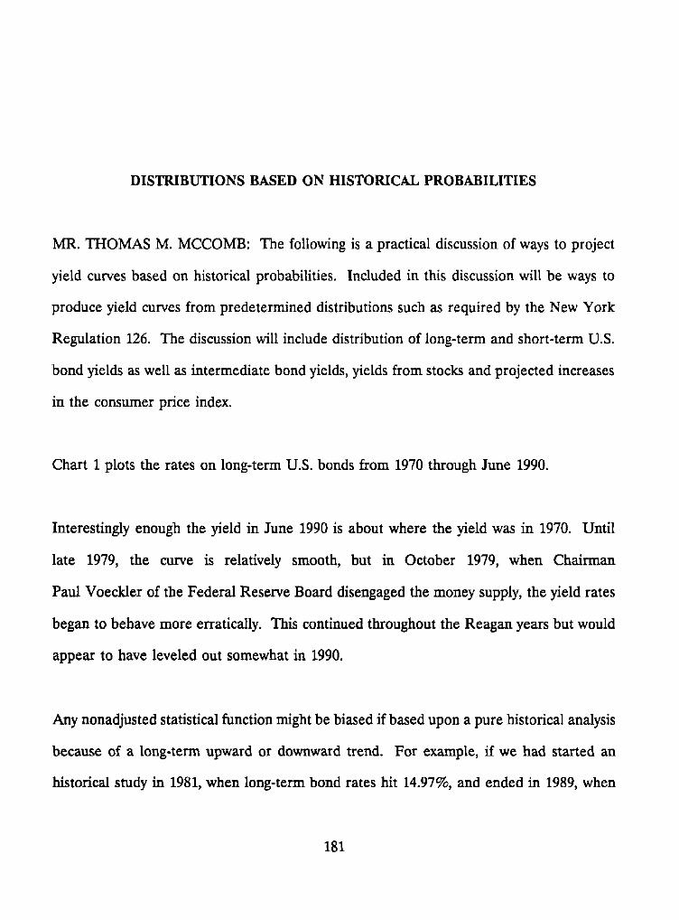
Our purpose is to find a variable for which we can compute the mean and standard
deviation. Once this variable is determined we can use the Knuth Method (Donald E.
Knuth, The Art of Computer Programming). This procedure is described in the cookbook
included at the end of my presentation.
The resulting variable is relatively random as illustrated by the following histogram in
Chart 2.
Short-term bond yields, based on the 90-day bond rate, can be compared with long-term
rates as shown in Chart 3. Here the difference between the short-term rates and the long-
term bond rates are the "hairs" on the curve. It is logical to assume that the magnitude
of the difference is related to the magnitude of the long-term bond rate. While there may
be a cyclical pattern, it is difficult to reduce this cyclical pattern to any reasonable formula.
183
1990 SYMPOSIUM FOR THE VALUATION ACTUARY
CHART 2
HISTOGRAM OF LONG-TERM YIELD DEVIATIONS
m m
m m
m m m
w
m
m m
w m
m
| | I i i i ' I I i i ' i . . . . i i I I i i I I
184
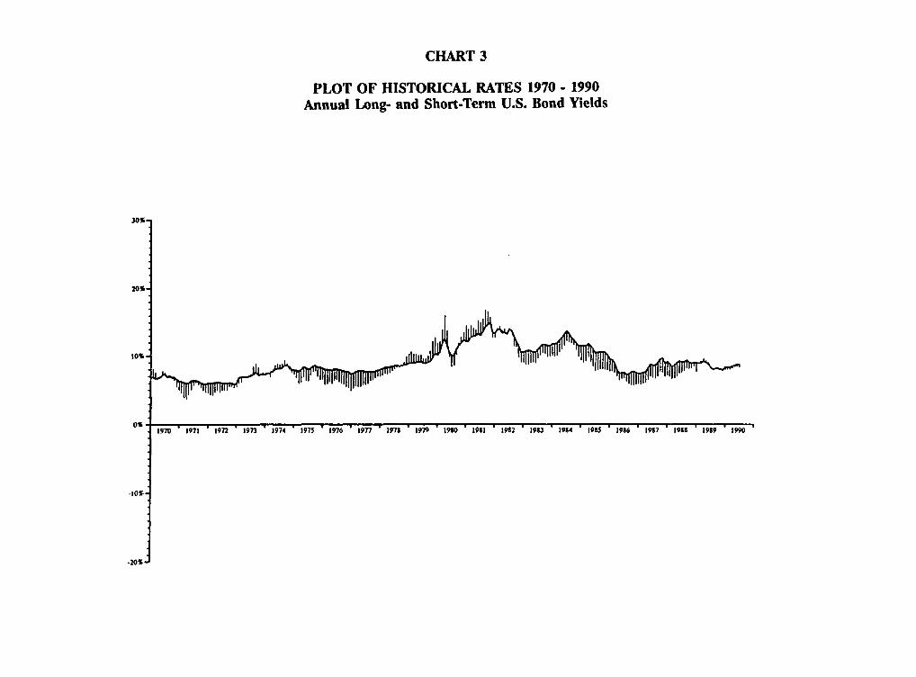
CHART 3
PLOT OF HISTORICAL RATES 1970 - 1990 Annual Long- and Short-Term U.S. Bond Yields
3011;-
2 0 S ,
1 0 % ,
O K 19"70 1971 1972 1973 " 1974 ' 1975 " 1976 ' 19"7"7 ' 15rTg " 1979 " 1980 " 1981 ' 1982 " 1983 1984 198.5 1986 ' 1987 " 1988 ' 1989 1990
-I0~-.

1990 SYMPOSIUM FOR THE VALUATION ACTUARY
Many argue that rate curve inversions are more apt to occur when rates are high. This was
true, of course, for the inversion that occurred from 1979 to 1981. But yield curves in 1973
and 1974 were not particularly high, and there was a yield curve inversion.
We ignore whether or not the curve is inverted and treat, as a variable, the absolute value
of the difference of the long-term rate and the short-term rate. We consider the ratio of
this absolute value to the long-term rate as a variable and find its mean and deviation. We
can then use Knuth's Method again to produce a set of projected values.
Since a normal noninverted curve tends to stay normal and an inverted curve tends to stay
inverted, although not at the same persistency, we can determine the probability that a
normal curve will not invert and the probability that an inverted curve will stay inverted.
For durations more than 90 days but less than 30 years, assume that the intervening rate
is the long-term rate plus or minus a portion of the absolute value of the difference
between the two rates. Assume also that the portion for any duration is an exponential
function given in the cookbook. We can then assume an exact fit for the values for one
year and determine the value of A and B sufficient to produce a complete yield curve as
described in the cookbook.
186
YIELD CURVE PROJECTION TECHNIQUES
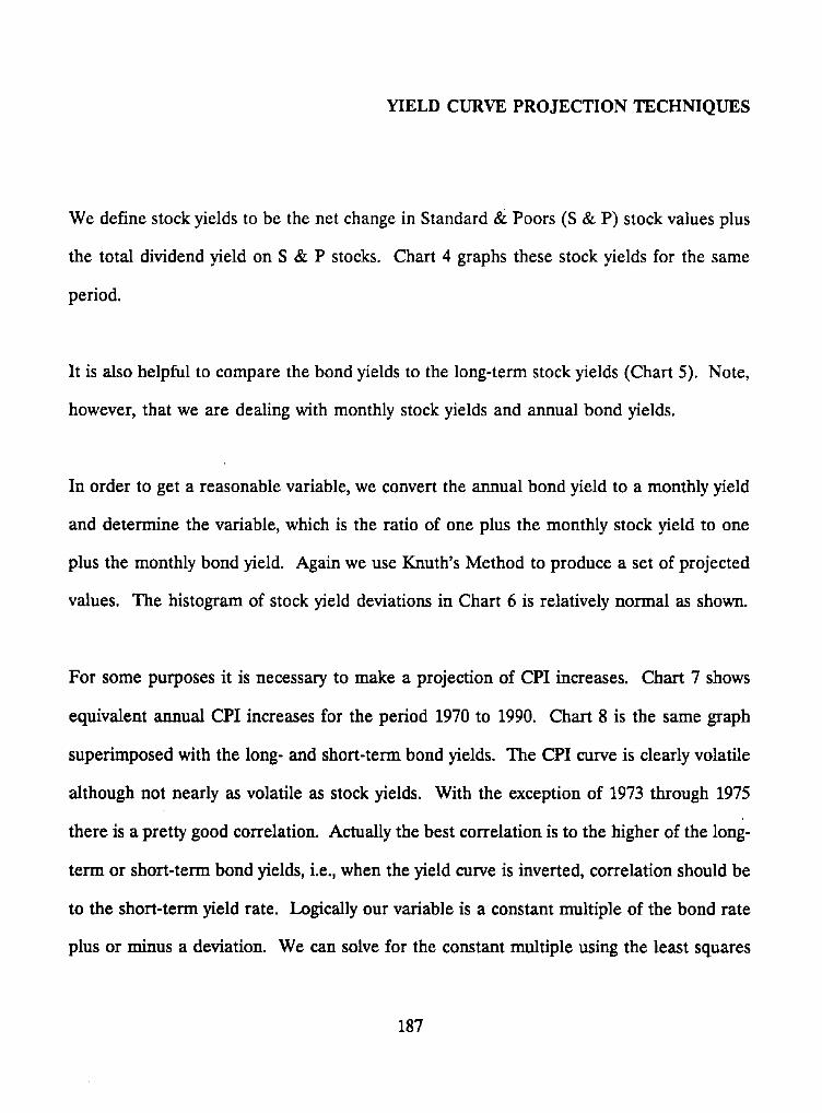
We define stock yields to be the net change in Standard & Poors (S & P) stock values plus
the total dividend yield on S & P stocks. Chart 4 graphs these stock yields for the same
period.
It is also helpful to compare the bond yields to the long-term stock yields (Chart 5). Note,
however, that we are dealing with monthly stock yields and annual bond yields.
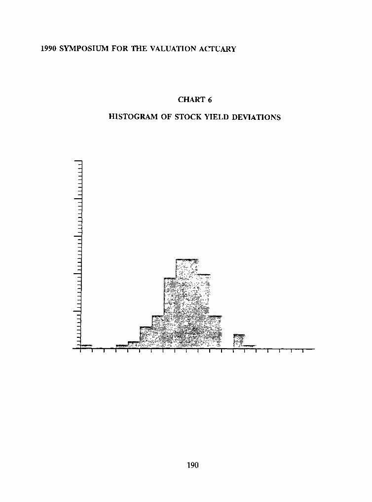
In order to get a reasonable variable, we convert the annual bond yield to a monthly yield
and determine the variable, which is the ratio of one plus the monthly stock yield to one
plus the monthly bond yield. Again we use Knuth's Method to produce a set of projected
values. The histogram of stock yield deviations in Chart 6 is relatively normal as shown.
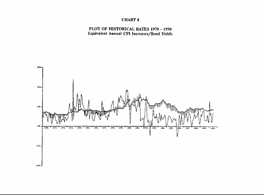
For some purposes it is necessary to make a projection of CPI increases. Chart 7 shows
equivalent annual CPI increases for the period 1970 to 1990. Chart 8 is the same graph
superimposed with the long- and short-term bond yields. The CPI curve is clearly volatile
although not nearly as volatile as stock yields. With the exception of 1973 through 1975
there is a pretty good correlation. Actually the best correlation is to the higher of the long-
term or short-term bond yields, i.e., when the yield curve is inverted, correlation should be
to the short-term yield rate. Logically our variable is a constant multiple of the bond rate
plus or minus a deviation. We can solve for the constant multiple using the least squares
187
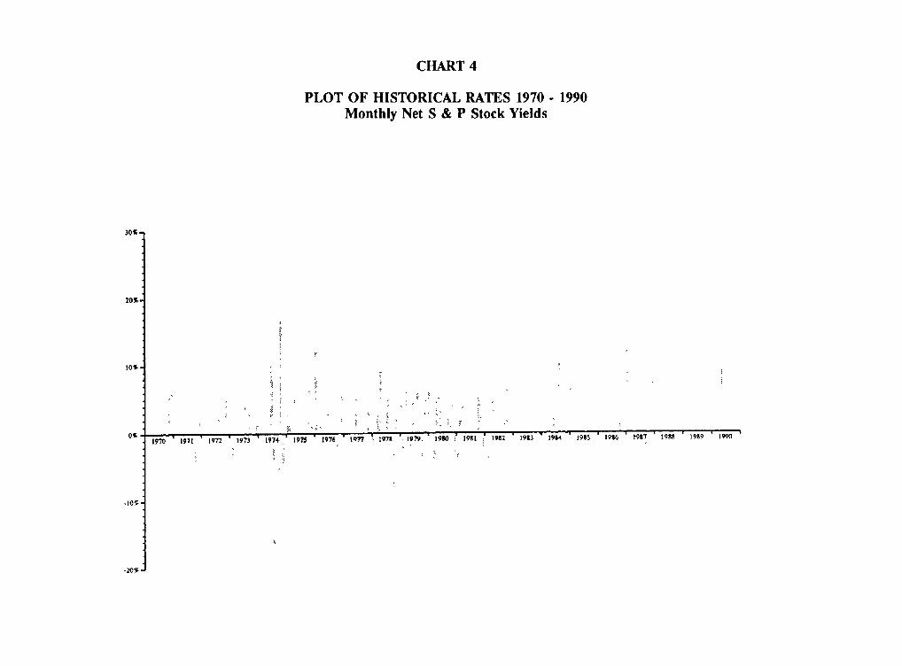
CHART 4
PLOT OF HISTORICAL RATES 1970 - 1990 Monthly Net S & P Stock Yields
30~t-
20%,
I 0 ~
O~
-209~
CHART 5
PLOT OF HISTORICAL RATES 1970 - 1990 Monthly Net S & P Stock Yields/Long-Term Bond Yields
30~o
I 0 ~ ,
O~
- I 0 ~ •
- 20~ -
~ I~1"~ .~'.
~ ~ ~ ! I ~
1990 SYMPOSIUM FOR THE VALUATION ACTUARY
CHART 6
HISTOGRAM OF STOCK YIELD DEVIATIONS
m
2 ..4
m
I I i I I 1 I I I i ...... I ..... I I' . . . . . . . . I ..... I I i I i
190

CHART 7
PLOT OF HISTORICAL RATES 1970 - 1990 Equivalent Annual CPI Increases
2o~t-[
10~, I ~ _ -.~,. 0~ ~191D 19S4 I~ID ~ ! ' 1990
-10~..
-20Sl
20~-,J
PLOT OF HISTORICAL RATES 1970 - 1990 Equivalent Annual CPI Increases/Bond Yields
I0~.
01;, 1 9 7 0 • 1 9 7 | 1 9 7 2 1 9 7 3 | 9 7 4 • 1 9 7 5 | 9 7 6 • 1 9 T 7 | 9 7 8 ' 1 9 7 9 1 9 8 0 • f ' ' • •
- I 0 ~ •
-20~ i
CHART 8
YIELD CURVE PROJECTION TECHNIQUES
method and treat the deviation as a variable. We can then determine the mean and
standard deviation of this variable and use Knuth's Method to produce projected values.
It is possible to plot bond yields, stock yields and equivalent CPI increases. Chart 9 is an
historical plot of these rates for the period 1970 to 1990. The primary purpose of this
graph is to compare with projected graphs in the future.
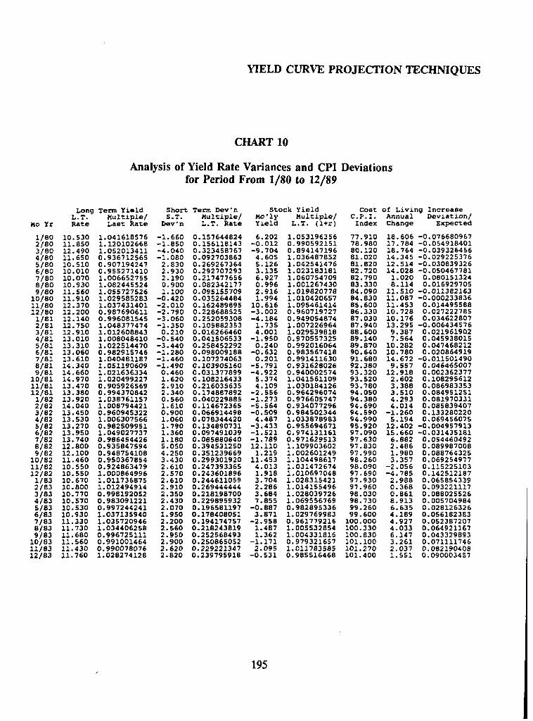
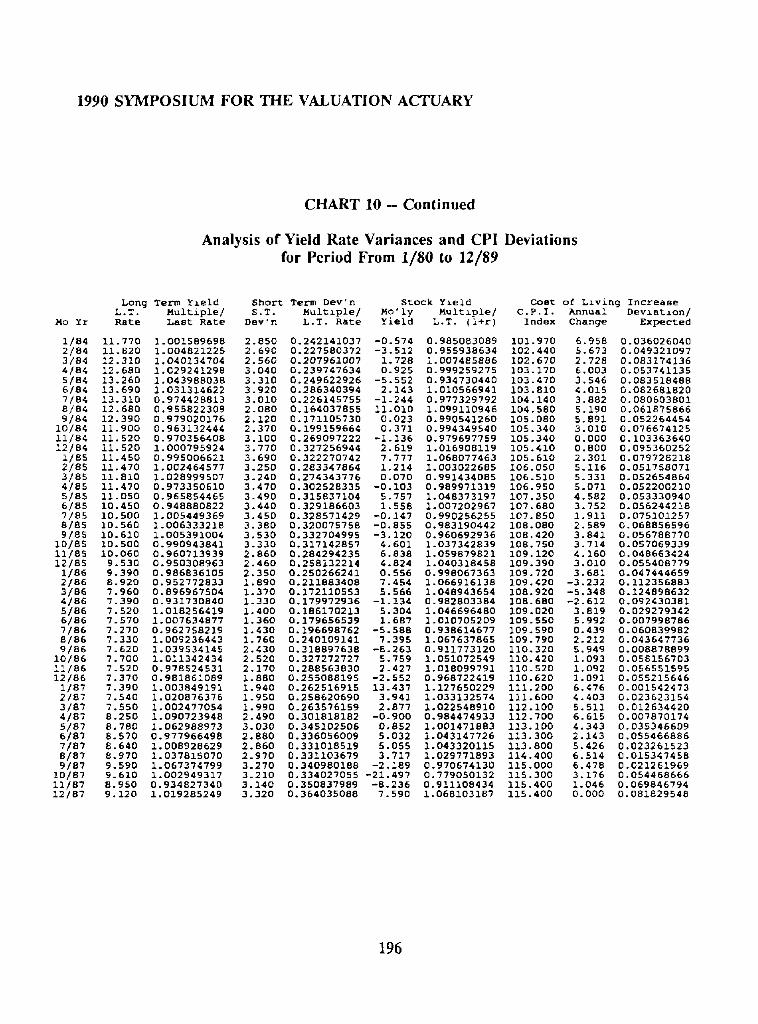
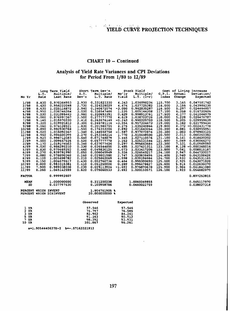
Finally I show in tabular form, the analysis of yield rate variances and CPI deviations for
the period from January 1, 1980 to December of 1989 (Chart 10). All factors and constants
and observed and expected values of intermediate bond yields are also shown.
In making the historical study I chose to take the 10-year period beginning in 1980.
work was actually completed for a December 1989 study.
This
In the case of the seven prescribed trims for New York, the long-term bond yield rate is
not stochastically projected but is predetermined. The NAIC Model Act makes similar
provision for some studies. Nevertheless, the other rates for these predetermined scenarios,
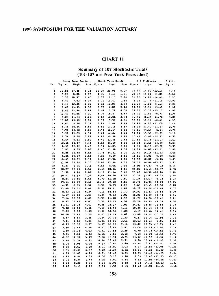
that is, the short-term rates, stock rates and CPI rates need to be stochastically projected.
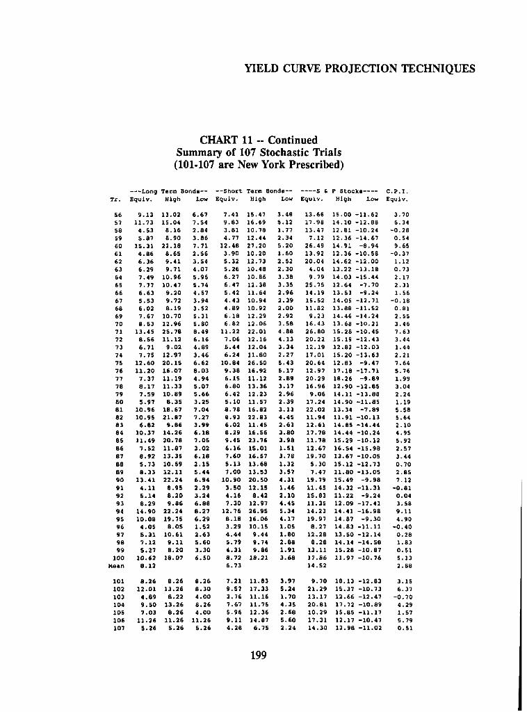
Chart 11 shows a summary of 107 stochastic trials, the last seven of which are in accordance
with the New York regulation.
193
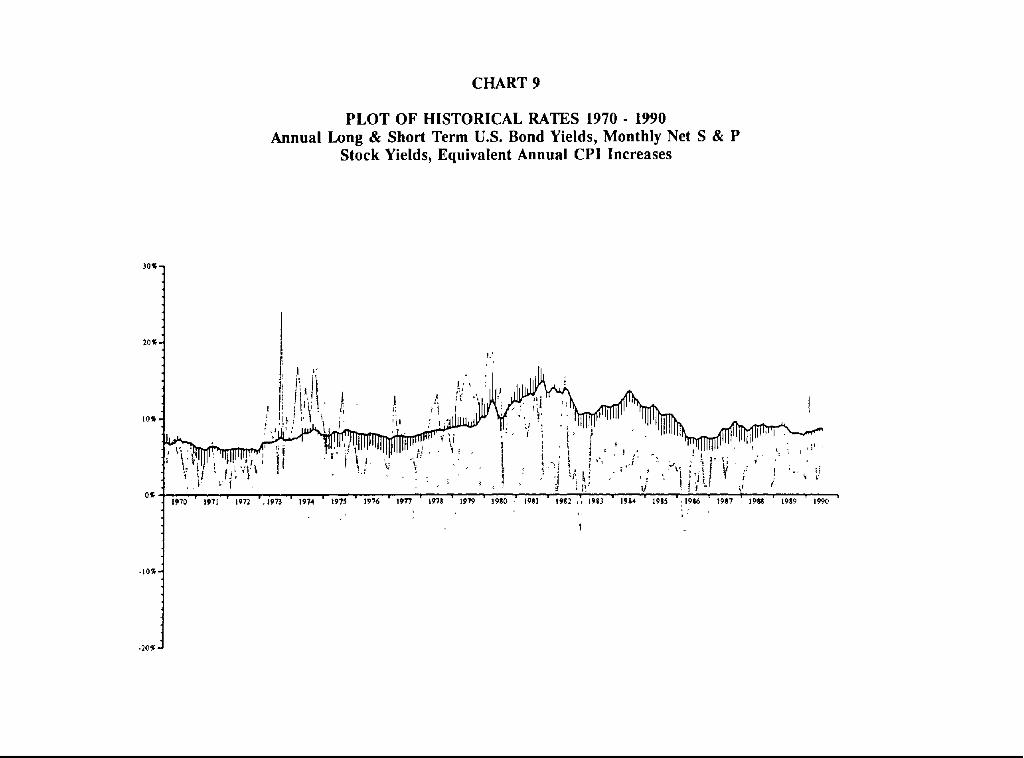
CHART 9
PLOT OF HISTORICAL RATES 1970 - 1990 Annual Long & Short Term U.S. Bond Yields, Monthly Net S & P
Stock Yields, Equivalent Annual CPI Increases
3 0 9 -
! 2OT. I
~f i " '/' I, ,
I, I ,t! ! .~ ¢ . ' , i l l l ~ I F , . , [ n - ~ : } l l _ ~ ! , ti ;!Jli ' " ! / i I
0% 1970 1971 1972 " ,197~ ' 1974 ' 1975' " i976 l 1 9 ~ I 1 ~ 8 l 1979 • 1980 -" 198| " 1 ~ 2 ,~ 1983 " 19114 ' 1985 l !1~8~ ' 1987 1911~ 1989 t990
- l O T
-20T
YIELD CURVE PROJECTION TECHNIQUES
CHART 10
Analysis of Yield Rate Variances and CPI Deviations for Period From 1/80 to 12/89
Mo Yr
118o 2/80 3/80 418o 5/8o 6•80 7/80 8/8o 918o
10180 11/8o 12/8o
1/81 2/81 3/81 4181 5/81 6/81 7181 8/81 9/81
10/81 11/81 12/81 1182 2/82 3/82 4/82 5•82 6/82 7/82 8/82 9/82
10/82 11182 12/82
1183 2/83 3/83 4/83 5/83 6/83 7183 8/83 9/83
lo/83 11183 12/83
Long L.T. Rate
10. 530 11.850 12.490 11.650 10.510 10.010 10,070 10.930 11.560 11.910 12.370 12.200 12.140 12.750 12.910 13.010 13.310 13. 060 13.610 14.340 14.660 14.970 13,470 13.380 13.920 14. 040 13.450 13.530 13.270 13.950 13. 740 12.800 12. 100 11.460 10.550 10,550 10.670 10,800 10,770 10.570 10.530 10.930 11.330 11.730 11.680 11.560 11.430 11,760
Term Yield Multiple/ Last Rate
1.041618576 1.120102668 1.052013411 0.936712565 0.907194247 0.955271410 1.006652755 1.082445524 1.055727526 1.029585283 1.037431401 0.987690611 0.996081545 1.048377474 1.012608843 1.008048410 1.022514470 0.982915746 1.040481187 1.051190609 1.021636334 1.020499227 0.905926569 0.994370842 1.038761157 1.008794421 0.960945322 1.006307566 0.982509951 1.049027737 0.986454426 0.935847594 0.948754108 0.950367854 0.924863479 1.000864996 1.011736875 1.012494914 0.998192052 0.983091221 0.997244241 1.037135940 1.035720946 1.034406258 0.996725111 0.991001464 0.990078076 1.028274128
Short: Term Dev'n Stock Yield Cost S.T. Multiple/ Mo'ly Multiple/ C.P.I.
Dev'n L.T. RaUe Yield L.T. (l÷r) ~ndex
-1.660 0.157644824 6.202 1.053196356 77.910 -1.850 0.156118143 -0.012 0.990592151 78.980 -4.040 0.323458767 -9.704 0.894147196 80.120 -1.080 0.092703863 4.605 1.036487852 81,020 2.830 0.269267364 5.126 1.042541476 81.820 2.930 0.292707293 3,135 1.023183181 82.720 2.190 0.217477656 6.927 1.060754709 82.790 0.900 0.082342177 0.996 1.001267430 83.330 i. I00 0.095155709 2.916 1.019820778 84.090
-0.420 0.035264484 1.994 1.010420657 84.830 -2.010 0.162489895 10.616 1.095461414 85.600 -2.790 0.228688525 -3.002 0.960719727 86.330 -3.060 0.252059308 -4,184 0.949054874 87.030 -1,350 0.105882353 1.735 1.007226964 87.940 0.210 0.016266460 4.001 1.029539818 88.600
-0.540 0.041506533 -1.950 0.970557325 89.140 -3.440 0.258452292 0.240 0.992016064 89.870 -1.280 0.098009188 -0.632 0.983567418 90.640 -1.460 0.107274063 0,201 0.991411630 91.680 -1.490 0.103905160 -5.791 0.931628026 92.380 0.460 0.031377899 -4.922 0.940002574 93.320 1.620 0.108216433 5.374 1.041561109 93.520 2.910 0.216035635 4,109 1.030184126 93.780 2.340 0.174887892 -2.556 0.964296074 94.050 0,560 0.040229885 -1.273 0.976605747 94.380 1.610 0.114672365 -5.564 0.934077296 94.690 0.900 0.066914498 -0.509 0.984502344 94.590 1.060 0.078344420 4.487 1.033878983 94,990 1.790 0.134890731 -3.433 0.955694671 95.920 1.360 0.097491039 -1.521 0.974131161 97.090 1.180 0.085880640 -1.789 0.971629513 97.630 5.050 0.394531250 12.110 1.109903602 97.830 4.250 0.351239669 1.219 1.002601249 97.990 3,430 0.299301920 11.453 1.104498617 98.260 2.610 0.247393365 4.013 1.031472674 98.090 2.570 0.243601896 1.918 1.010697048 97,690 2.610 0.244611059 3.704 1.028315421 97.930 2.910 0.269444444 2.286 1.014155496 97.960 2.350 0.218198700 3.684 1.028039726 98,030 2.430 0.229895932 7,855 1.069556769 98.730 2.070 0.196581197 -0.887 0.982895336 99.260 1.950 0.178408051 3.871 1.029769983 99.600 2,200 0.194174757 -2.958 0.961779216 I00.000 2.560 0.218243819 1.487 1.005532854 100.330 2.950 0.252568493 1.362 1.004331816 100.830 2.900 0.250865052 -1.171 0.979321657 101.100 2.620 0.229221347 2.095 1.011783585 101.270 2.820 0.239795918 -0.531 0.985516468 101,400
of Living Increase Annual Deviation/ Change Expected
18.606 -0.076680967 17,784 -0.054918401 18.764 -0.039326456 14.345 -0,029225376 12.514 -0.030839326 14.028 -0,050467781 1.020 0.080151324 8.114 0,016929705
11.510 -0.011382163 11,087 -0.000233836 11.453 0.014495588 10.728 0.027222785 10.176 0.034622807 13,295 -0.006434576 9.387 0,021961902 7.564 0.045938015
10.282 0.047468212 10.780 0.020864919 14.672 -0,011501490 9.557 0,046465007
12.918 0.002362377 2.602 0.108295612 3.388 0,086983353 3.510 0.084951251 4.293 0,081970331 4.014 0.085839407
-1.260 0.133280220 5.194 0,069456075
12,402 -0,004957913 15.660 -0.031435181 6.882 0,054460492 2.486 0.089987008 1.980 0.088764325 3.357 0.069254977
-2 .056 0.115225103 -4,785 0.142512187 2.988 0.065854339 0.368 0.093221117 0.861 0.088025526 8.913 0.005704984 6.635 0.028126326 4.189 0.056182383 4.927 0.052387207 4.033 0.064921167 6.147 0.043329893 3.261 0,071111746 2.037 0.082190408 1.551 0,090003457
195 F
1990 SYMPOSIUM FOR THE VALUATION ACTUARY
CHART 10 -- Continued
Analysis of Yield Rate Variances and CPI Deviations for Period From 1/80 to 12/89
Mo Yr
1/84 2/84 3/84 4 /84 s / 8 4 6 /84 7184 8184 9184
10/84 11/84 12/84 1/85 2/85 3185 4/85 5185 6/85 7185 8185 9/85
lO/8S 11/85 12/85 1/86 2/86 3/86 4 /86 5/86 6/86 7186 8/86 9/86
10/86 11/86 12/86 1/87 2/87 3/87 4/87 5/87 6/87 7/87 8187 9187
10/87 ii/87 12187
Long Term Yield L.T. Multiple/ Rate Last Rate
11.770 1.001589698 11.820 1.004821225 12.310 1.O40134704 12.680 1.029241298 13.260 1.043988038 13.690 1.031314622 13.310 0.974428813 12.680 0.955822309 12.390 0.979020176 11.900 0.963132444 11.520 0.970356408 11.520 1.000795924 11.450 0.995006621 11.470 1.002464577 11.810 1.028999507 11.470 0.973350610 11.050 0.965854465 10.450 0.948880822 10.500 1.005449369 10.560 1.006333218 10.610 1.005391004 10.500 0.990943841 10.060 0.960713939 9.530 0.950308963 9.390 0.986836105 8.920 0.952772833 7.960 0.896967504 7.390 0.931730840 7.520 1.018256419 7.570 1.007634877 7.270 0.962758219 7.330 1.009236443 7.620 1.039534145 7.700 1.011342434 7.520 0.978524531 7.370 0.981861089 7.390 1.003849191 7.540 1.020876376 7.550 1.002477054 8.250 1.090723948 8.780 1.062988973 8.570 0.977966498 8.640 1.008928629 8.970 1.037815070 9.590 1.067374799 9.610 1.002949317 8.950 0.934827340 9.120 1.019285249
Short Term Dev'n Stock Yxeld Cost S.T. Multaple/ Mo'ly Multlple/ C.P.I.
Dev'n L.T. Rate Yield L.T. (l+r) Index
2.850 0.242141037 -0.574 0.985083089 101.970 2.690 0.227580372 -3.512 0.955938634 102.440 2.560 0.207961007 1.728 1.007485886 102.670 3.040 0.239747634 0.925 0.999259275 103.170 3.310 0.249622926 -5.552 0.934730440 103.470 3.920 0.286340394 2.143 1.010566941 103.810 3.010 0.226145755 -1.244 0.977329792 104.140 2.080 0.164037855 ii.010 1.099110946 104.580 2.120 0.171105730 0.023 0.990541260 105.080 2.370 0.199159664 0.371 0.994349540 105.340 3.100 0.269097222 -1.136 0.979697759 105.340 3.770 0.327256944 2.619 1.016908119 105.410 3.690 0.322270742 7.777 1.068077463 105.610 3.250 0.283347864 1.214 1.003022685 106.050 3.240 0.274343776 0.070 0.991434085 106.510 3.470 0.302528335 -0.103 0.989971319 106.950 3.490 0.315837104 5.757 1.048373197 107.350 3.440 0.329186603 1.558 1.007202967 107.680 3.450 0.328571429 -0.147 0.990256255 107.850 3.380 0.320075758 -0.855 0.983190442 108.080 3.530 0.332704995 -3.120 0.960692936 108.420 3.330 0.317142857 4.601 1.037342839 108.750 2.860 0.284294235 6.838 1.059879821 109.120 2.460 0.258132214 4.824 1.040318458 109.390 2.350 0.250266241 0.556 0.998067363 109.720 1.890 0.211883408 7.454 1.066916138 109.420 1.370 0.172110553 5.566 1.048943654 108.920 1.330 0.179972936 -1.134 0.982803384 108.680 1.400 0.186170213 5.304 1.046696480 109.020 1.360 0.179656539 1.687 1.010705209 109.550 1.430 0.196698762 -5.588 0.938614677 109.590 1.760 0.240109141 7.395 1.067637865 109.790 2.430 0.318897638 -8.263 0.911773120 110.320 2.520 0.327272727 5.759 1.051072549 110.420 2.170 0.288563830 2.427 1.018099791 110.520 1.880 0.255088195 -2.552 0.968722419 110.620 1.940 0.262516915 13.437 1.127650229 111.200 1.950 0.258620690 3.941 1.033132574 111.600 1.990 0.263576159 2.877 1.022548910 112.100 2.490 0.301818182 -0.900 0.984474933 112.700 3.030 0.345102506 0.852 1.001471883 113.100 2.880 0.336056009 5.032 1.043147726 113.300 2.860 0.331018519 5.055 1.043320115 113.800 2.970 0.331103679 3.717 1.029771893 114.400 3.270 0.340980188 -2.189 0.970674130 115.000 3.210 0.334027055 -21.497 0.779050132 115.300 3.140 0.350837989 -8.236 0.911108434 115.400 3.320 0.364035088 7.590 1.068103187 115.400
of Living Increase Annual Devxatxon/ Change Expected
6.958 0.036026040 5.673 0.049321097 2.728 0.083174136 6.003 0.053741135 3.546 0.083518488 4.015 0.082681820 3.882 0.080603801 5.190 0.061875866 5.891 0.052264454 3.010 0.076674125 0.000 0.103363640 0.800 0.095360252 2.301 0.079728218 5 116 0.051758071 5 331 0.052654864 5 071 0.052200210 4 582 0.053330940 3 752 0.056244218 i 911 0.075201257 2 589 0.068856596 3 841 0.056788770 3 714 0.057069339 4 160 0.048663424 3 010 0.055408779 3.681 0.047444659
-3.232 0.112356883 -5.348 0.124898632 -2.612 0.092430381 3.819 0.029279342 5.992 0.007998786 0.439 0.060839982 2.212 0.043647736 5.949 0.008878899 1.093 0.058156703 1.092 0.056551595 1.091 0.055215646 6.476 0.001542473 4.403 0.023623154 5.511 0.012634420 6.615 0.007870174 4.343 0.035346609 2.143 0.055466886 5.426 0.023261523 6.514 0.015347458 6.478 0.021261969 3.176 0.054468666 1.046 0.069846794 0.000 0.081829548
196
' :"YIELD cURVE PROJECTION TECHNIQUES
CHART 10 -- Continued
Analysis of Yield Rate Variances and CPI Deviations for Period From 1/80 to 12/89
Long Term Yield Short Term Dev°n Stock Yield L.T. Multiple/ S.T. Multiple/ Mo'ly Multiple/
Mo ¥r RaUe Last Rate Dev'n L.T. Ra~e Yield L.T. (ler)
1/88 8.830 0.970364953 2.930 0.331823330 4.343 1.036098234 2/88 8.420 0.956222048 2.730 0.324228029 4.474 1.037725382 3/88 8.630 1.025116872 2.940 0.340672074 -3.050 0.962835287 4/88 8.950 1.036746364 3.030 0.338547486 1.235 1.005144308 5/88 9.230 1.031095443 2.960 0.320693391 0.629 0.998913761 6/88 9.000 0.976997367 2.500 0.277777778 4.619 1.038703726 7/88 9.140 1.015970230 2.410 0.263676149 -0.243 0.990325703 8/88 9.320 1.019921813 2.300 0.246781116 -3.554 0.957324673 9/88 9.060 0.974128521 1.830 0.201986755 4.275 1.035240866
10/88 8.890 0.982930784 1.550 0.174353206 2.892 1.021643264 11/88 9.020 1.015092367 1.340 0.148558758 -1.587 0.977072874 12/88 8.960 0.994600399 2.270 0.253348214 1.770 1.010448500 1/89 8.920 0.996712083 0.640 0.071748879 3.445 1.027110576 2/89 9.000 1.009647526 0.520 0.057777778 3.252 1.025131546 3/89 9.170 1.019174503 0.340 0.037077426 0.297 0.995663684 4/89 9.030 0.986295210 0.330 0.036544850 3.485 1.027421311 5/89 8.830 0.979669252 0.440 0.049830125 4.073 1.033417206 6/89 8.270 0.939791990 0.050 0.006045949 3.336 1.026540217 7/89 8.080 0.978890368 0.160 0.019801980 2.747 1.020838496 8/89 8.120 1.005898782 0.210 0.025862069 4.598 1.039196984 9/89 8.150 1.004679617 0.430 0.052760736 0.484 0.998300690
10/89 8.000 0.983315381 0.410 0.051250000 0.289 0.996478627 11/89 7.900 0.989038038 0.230 0.029113924 -1.692 0.976870678 12/89 8.260 1.045142559 0.620 0.075060533 2.692 1.020150571
FACTOR 0.999992807
MEAN 1.000000000 0.211200238 1.0060349855 SD 0.037797630 0.100958786 0.0460022759
PERCENT WHICH INVERT 1.904761905 • PERCENT WHICH DISINVERT 20.000000000 •
Observed Expected
1 YR 57.546 57.546 2 YR 76.797 76.586 3 YR 82.962 84.241 5 YR 91.163 90.913 7 YR 98.392 93.931
i0 YR 101.867 96.261
a-l.9054440637E-2 b--.57163321913
Cost of Living Increase C.P.I. Annual Deviation/ lndex Change Expected
115.700 3.165 0.047581742 116.000 3.156 0.043986230 116.500 5.297 0.024464857 117.100 6.358 0.016720606 117.500 4.177 0.041046979 118.000 5.228 0.028476787 118.500 5.205 0.029959639 119.000 5.182 0.031799434 119.800 8.372 -0.002431778 120.200 4.081 0.038955051 120.300 1.003 0.070903125 120.500 2.013 0.060260382 121.100 6.141 0.018620202 121.600 5.069 0.030066272 122.300 7.131 0.010969590 123.100 8.138 -0.000360016 123.800 7.041 0.008815187 124.100 2.947 0.044733017 124.400 2.940 0.043100426 124.700 2.933 0.043531165 125.000 2.925 0.043871828 125.600 5.915 0.012635070 125.900 2.904 0.041841080 126.100 1.923 0.054882979
0.897253815
0.045117970 0.038827318
197
1990 SYMPOSIUM FOR THE VALUATION ACTUARY
CHART 11
Summary of 107 Stochastic Trials (101-107 are New York Prescribed)
---Long Term Bonds .... Short Term Bonds ...... 5 &
Tr. Equiv. High Low Equiv. High Low Equiv.
1 12.81 17.45 8.33 11.00 21.06 5.05 ]8.90
2 5.26 8.80 2.97 4.35 9.38 1.81 20.72
3 7.33 10.97 5.40 6.07 11.17 2.96 11.92
4 4.42 7.93 3.09 3.71 11.47 1.86 6.25
5 7.15 12.85 2.75 5.78 12.00 1.74 20.92
6 8.67 13.93 4.30 6.87 14.02 2.40 13.08
7 9.42 12.94 6.69 7.48 15.29 4.06 17,75
8 10,48 15.86 7.00 8.79 16.47 4.47 18.70
9 8.09 11,64 6.26 6.68 12.06 3.73 10.48
I0 10.08 13.49 7.24 8.17 17.95 4.66 10.72
11 6.67 8.76 5.29 5.92 11.45 3.49 11.93
12 8.16 10.85 5.53 6.52 11.18 3.57 11.35
13 9.98 14.50 6.80 8.54 16.69 3.84 15.66
14 7.92 12.09 4,14 6.69 14.44 2.44 11.24
15 5.74 8.38 3,91 4.86 10.58 2.63 10.44
16 6.64 9.61 3.89 5.41 12.58 2.43 10.61
17 10.48 14.47 7,41 8.63 15.69 4.98 11.14
18 8.55 12.92 6,48 7.14 14.03 3.61 7.91
19 7.81 9.59 5.88 6.40 11.58 4.07 14.24
20 8.88 11.40 6.66 7,76 14.62 4.00 22.47
21 5.25 10.57 2.56 4.26 9.59 1.53 11.60
22 10.61 16.57 5.11 8,83 17.96 4.01 19.55
23 1 2 . 8 5 2 2 . 3 4 8 .33 10 ,92 2 2 . 2 5 4 . 1 5 2 1 . 1 8 24 5.31 8.66 3.41 4,51 8.96 2.08 15.06
25 10.27 15.93 6.52 8,40 18.16 4.57 21.08
26 7.35 9.14 6.06 6.11 11.16 3.68 25.66
27 10.42 18.13 7.29 8.45 18.60 5.04 22.36
28 8 . 2 4 1 0 . 6 6 5 .58 6 . 7 0 12 .28 3 . 8 0 17 .34 29 19.14 26.39 8.60 16.10 29.92 5.83 31.76
30 4.92 8.85 2.34 3.98 9.59 1.28 5.03
31 12.49 16.71 8.41 10.31 19.81 5.81 19.72
32 8.53 12.32 6.34 7.11 14.63 3.30 14.02
33 6 .17 1 0 . 8 8 3 . 5 7 5 .44 9 . 9 2 2 .02 16 .81 34 7.14 10.33 4.49 5.93 11.70 2.95 12.71
35 9.92 13.45 6.87 7.75 12.57 4.56 20.26
36 11.51 18.38 4.63 9.25 22.27 3.01 24.42
37 9 . 1 8 11 .53 6 . 5 8 7 .69 1 4 . 4 3 4 . 1 3 1 0 . 3 8 38 2 . 8 3 7 . 9 3 1 . 5 0 2 . 3 1 1 0 . 3 0 1 .00 4 . 1 9 39 1 0 . 6 6 15 .63 7 . 2 5 8 . 8 3 13 .79 5 .09 1 3 . 8 8 40 4.47 8.57 2.15 3.64 10.72 1.20 6.27
41 7.21 9.66 5.01 6.01 12.00 3.51 12.53
42 6 . 2 3 1 0 . 1 6 3 . 2 7 5 .19 1 0 . 7 8 2 . 1 6 13.42 43 7.56 11.46 4.15 6.67 13.82 2.97 13.08
44 5.69 11.21 4.03 4.71 10.64 2.29 6.70
45 7.05 9.32 4.33 5.65 9.68 2.68 7.50
46 8 . 5 2 12 .31 5 . 9 9 7 . 0 6 1 5 . 3 4 3 . 7 5 2 1 . 7 2 47 7 . 4 8 1 1 . 3 9 4 . 2 2 6 .24 13 .45 2 . 7 2 9 . 5 0 48 6 . 2 6 9 . 0 6 4 . 0 4 5 .27 1 0 . 9 4 2 . 4 0 12 .15 49 3.50 8.62 1.58 3.01 11.00 1.03 9.97
50 B.95 12.39 6.37 7.22 15.24 3,78 13.54
51 7 , 9 3 11 .65 4 . 7 3 6 . 5 1 1 1 . 4 8 3 . 0 3 18 .39 52 4 . 6 1 8 . 5 4 3 .32 4 , 0 0 10 .13 1 . 9 0 5 .05 53 3.75 8.24 1.43 3.15 9.92 0.94 9.53
54 6 . 2 1 8 . 8 8 3 .71 8 .25 1 1 . 9 9 2 . 1 8 8 .94 55 6 . 6 8 9 . 1 1 4 . 9 6 5 .39 9 . 9 9 2 . 8 3 1 4 . 2 0
P Stocks .... High Low
]4.00 -12.14
15.24 -11.83
14.08 -14.41
12.74 -11.19
13.86 -11.63
12.93 -13.45
13. 19 -15. 12
13.99 -9.71
15.34 -11.78
12.57 -8.61
14.95 -11.00
11 .40 - 1 1 . 1 7 13 .67 - 8 . 9 3 13 .53 -12.29
13.62 -15.27
13. 16 -11.07
14.65 -14.09
18.15 -12.22
14.08 - 1 2 . 5 1 15.14 -11.73
14.92 -9.79
18.02 -9.28
16.86 -12.92
17.47 -9.22
14.14 -10.07
16.98 -10.90
22.87 -9.32
13.07 -9.93
15.26 -14. lO
12.15 -12.50
15.68 -12.44
11.63 -17.52
14.39 -13.79
14.36 -12.46
16.15 -9.79
13.55 -11.64
15.04 -14.42
1 1 . 7 6 - 1 4 . 4 8 14.52 - 1 0 . 3 3 1 1 . 0 4 - 1 0 . 9 3 1 3 . 7 ] - 9 . 9 2 12 .65 - 1 3 . 2 7 16 .83 - 1 0 . 9 7 17.03 -14.53
16.80 -11.64
13.52 -11.52
13.44 -15.97
1 3 . 8 0 - 1 1 . 6 2 11 .89 - 1 2 . 9 6 12 .32 - 1 3 . 4 2 14 .45 - 1 4 . 2 3 18 .48 -11.73
13.85 - 1 4 . 0 6 14 .18 - 1 2 . 2 3 14 .04 - 1 1 . 5 5
198
C.P.l.
Equlv.
7.44
-0.04
2.50
-0.93
2.07
2.99
4.07
5.24
3,00
4.50
1.46
2.76
4.70
3.18
0.72
1.53
5.04
3.33
2.45
3.68
-0.01
5.45
7.32
0.35
4.80
2.18
4 . 9 8 2.92
12.65
0.18
7.07
3.29
1.06
2.11
4.20
6.09
4.05
-2.15
5.46
-0.31
1.80
1.46
2.71
0.72
1.76
3.14
2.38
0.89
-1.28
3.46
2.84
-0.13
-1.60
1.33
1.58
YIELD CURVE PROJECTION TECHNIQUES
CHART 11 - - Continued Summary of 107 Stochastic Trials (101-107 are New York Prescribed)
---Long Term Bonda .... Short Term Bonda ...... S &
Tr. Equiv. H i g h Low Equiv. H i g h LOW Equiv.
56 9 . 1 3 13 .02 6 . 6 7 7 . 4 1 15 .47 3 . 4 8 1 3 . 6 6 57 1 1 . 7 3 15 .04 7 . 5 4 9 . 8 3 16 .69 5 .12 17 .98 58 4.53 8.16 2.84 3.81 10.78 1.77 13.47
59 8.87 8.90 3.86 4.77 12.44 2.34 7.12
60 1 5 . 3 1 2 2 . 1 8 7 . 7 1 1 2 . 4 8 2 7 . 2 0 5 . 2 0 2 6 . 4 9 61 4 . 8 6 8 . 6 5 2 . 5 6 3 . 9 0 10 .20 1 . 6 0 13 .92 62 6 . 3 6 9 . 4 1 3 . 5 4 5 .32 12 .73 2 . 5 2 2 0 . 0 4 63 6 . 2 9 9 . 7 1 4 . 0 7 5 . 2 6 10 .48 2 . 3 0 4 . 0 4 64 7 . 4 9 10 .96 5 . 9 5 6 . 2 7 10 .86 3 . 3 8 9 . 7 9 65 7.77 10.47 5.74 6.47 12.38 3.35 25.75
66 6 . 6 3 9 . 2 0 4 . 5 7 5 .42 11 .64 2 . 9 6 14 .19 67 5.53 9.72 3.94 4.43 10.94 2.39 15.52
68 6 . 0 2 8 . 1 9 3 . 5 2 4 . 8 9 10 .92 2 . 0 0 11 .82 69 7.67 10.70 5.31 6.18 12.29 2.82 9.23
70 8.53 12.96 5.80 6.82 12.06 3.58 16.43
71 1 3 . 4 5 2 5 . 7 8 8 . 4 9 11 .22 22 .01 4 . 8 8 2 6 . 8 0 72 8 . 5 6 11 .12 6 . 1 6 7 . 0 6 12 .16 4 . 1 3 2 0 . 2 2 73 6 . 7 1 9 . 0 2 4 . 8 9 5 . 4 4 12 .04 3 . 3 4 1 2 . 1 9 74 7 . 7 5 12 .97 3 . 4 6 6 .24 11 .80 2 . 2 7 17 .01 75 1 2 . 6 0 2 0 . 1 5 6 . 6 2 10 .84 2 6 . 5 0 5 . 4 3 2 0 . 6 4 76 1 1 . 2 0 16 .07 8 . 0 3 9 . 3 8 16 .92 5 . 1 7 12 .97 77 7 . 3 7 1 1 . 1 9 4 . 9 4 6 . 1 5 11 .12 2 . 8 9 2 0 . 2 9 78 8 . 1 7 11 .33 5 . 0 7 6 . 8 0 13 .36 3 . 1 7 1 6 . 9 6 79 7 . 5 9 1 0 . 8 9 5 . 6 6 6 . 4 2 12 .23 2 . 9 6 9 . 0 6 80 5 . 9 7 8 . 3 5 3 . 2 5 5 . 1 0 11 .57 2 . 3 9 17 .24 81 1 0 . 9 6 18 .67 7 . 0 4 8 . 7 8 16 .82 3.13 2 2 . 0 2 82 1 0 . 9 5 2 1 . 8 7 7 . 2 7 8 . 9 3 22 .83 4 . 4 5 11 .94 83 6 . 8 2 9 . 8 6 3 . 9 9 6 . 0 2 11 .45 2 . 6 3 1 2 . 6 1 84 1 0 . 3 7 1 4 . 2 6 6 . 1 8 8 . 2 9 16 .56 3 . 8 0 1 7 . 7 8 85 1 1 . 4 9 2 0 . 7 8 7 . 0 5 9 . 4 5 2 3 . 7 6 3 . 9 8 1 1 . 7 8 86 7 . 5 2 11 .87 3 . 0 2 6 . 1 6 15 .01 1 .51 12 .67 87 8 . 9 2 13.35 6 . 1 8 7 . 6 0 16 .57 3 . 7 8 1 9 . 7 0 88 5 . 7 3 10 .59 2 . 1 5 5 . 1 3 13 .68 1 . 3 2 5 . 3 0 89 8 .33 12 .11 5 . 4 4 7 . 0 0 13 .53 3 . 5 7 7 . 4 7 90 1 3 . 4 1 2 2 . 2 4 6 . 9 4 1 0 . 9 0 2 0 . 5 0 4 , 3 1 1 9 . 7 9 91 4 . 1 1 8 . 9 5 2 . 2 9 3 . 5 0 12 .15 1 . 4 6 1 1 . 4 5 92 5 . 1 4 8 . 2 0 3 . 2 4 4 . 1 6 8 . 4 2 2 . 1 0 15 .83 93 8 . 2 9 9 . 8 6 6 . 8 8 7 . 3 0 12 .97 4 . 4 5 1 1 . 3 5 94 1 4 . 9 0 2 2 . 2 4 8 . 2 7 1 2 . 7 6 26 .95 5 . 3 4 1 4 . 2 3 95 1 0 . 0 8 19 .75 6 . 2 9 8 . 1 8 16 .06 4 . 1 7 1 9 . 9 7 96 4 . 0 5 8 . 0 5 1 . 5 2 3 . 2 9 10 .15 1 .05 8 . 2 7 97 5 . 3 1 1 0 . 6 1 2 . 6 3 4 . 4 4 9 . 4 4 1 . 8 0 1 2 . 2 8 98 7 . 1 2 9 . 1 1 5 . 6 0 5 . 7 9 9 . 7 4 2 . 8 8 8 . 2 8 99 5 . 2 7 6 . 2 0 3 . 3 0 4 . 3 1 9 . 8 6 1 . 9 1 13 .11
100 1 0 . 6 2 1 8 . 0 7 6 . 5 0 8 . 7 2 18 .21 3 . 6 8 1 7 . 8 6 Mean 8 . 1 2 6 . 7 3 14 .52
101 8 . 2 6 8 . 2 6 8 . 2 6 7 . 2 1 11 .83 3 . 9 7 9 . 7 0 102 1 2 . 0 1 1 3 . 2 6 8 . 3 0 9 . 5 7 1"/ .33 5 . 2 4 2 1 . 2 9 103 4.89 8.22 4.00 3.76 11.16 1.70 13.17
104 9 . 5 0 13 .26 8 . 2 6 7 . 6 7 11 .75 4 . 3 5 2 0 . 8 1 105 7 . 0 3 8 . 2 6 4 . 0 0 5 . 9 6 12 .36 2 . 6 8 10 .29 106 1 1 . 2 6 1 1 . 2 6 1 1 . 2 6 9 . 1 1 14 .87 5 . 6 0 17 .31 107 5 . 2 6 5 . 2 6 5 . 2 6 4 . 2 8 6 . 7 5 2 . 2 4 1 4 . 3 0
P S t o c k i . . . . C . P . I . H i g h Low E q u i v .
15 .00 - 1 1 . 6 2 3 . 7 0 14 .10 - 1 2 . 8 8 6 .34 12 .81 - 1 0 . 2 4 - 0 . 2 8 12 .36 - 1 4 . 6 7 0 .54 14 .91 - 8 . 9 4 9 .65 12 .36 - 1 0 . 5 8 - 0 . 3 7 14 .62 - 1 2 . 0 0 1 .12 13 .22 - 1 3 . 1 8 0 . ' / 3 14 .03 - 1 5 . 4 4 2 .17 12 .64 - 7 . 7 0 2 .31 13.53 - 9 . 2 4 1 .56 14 .05 - 1 2 . 7 1 - 0 . 1 8 13 .88 - 1 1 . 5 2 0 . 8 1 14 .46 - 1 4 . 2 4 2 . 5 5 13 .68 - 1 0 . 2 1 3 . 4 6 15 .28 - 1 0 . 4 5 7 .63 15 .19 - 1 2 . 4 3 3 .44 12 .82 - 1 2 . 0 3 1 .44 1 5 . 2 0 - 1 3 . 6 3 2 .21 12 .83 - 9 . 4 7 7 . 6 4 17 .18 - 1 7 . 7 1 8 . 7 6 18 .26 - 9 . 8 9 1 .99 1 2 . 9 0 - 1 2 . 8 5 3 . 0 4 14 .11 - 1 3 . 8 8 2 . 2 4 1 4 . 9 0 - 1 1 . 8 5 1 .19 13.34 - 7 . 8 9 5 . 5 8 11 .91 - 1 0 . 1 3 5 .64 14 .85 - 1 4 . 4 4 2 . 1 0 1 4 . 4 4 - 1 0 . 2 4 4 . 9 5 15 .29 - 1 0 . 1 2 5 .92 1 6 . 5 4 - 1 5 . 9 8 2 . 5 7 1 3 . 6 7 - 1 0 . 0 5 3 . 4 4 15 .12 - 1 2 . 7 3 0 . 7 0 1 1 . 8 0 - 1 3 . 0 5 2 . 8 5 15.49 -9.98 7.12
14 .32 - 1 1 . 3 1 - 0 . 8 1 11 .22 - 9 . 2 4 0 . 0 4 12 ,09 - 1 7 . 4 1 3 . 5 8 14 ,41 - 1 6 . 9 8 9 . 1 1 14 .87 - 9 . 3 0 4 . 9 0 14 ,83 - 1 1 . 1 1 - 0 . 4 0 1 3 , 5 0 - 1 2 . 1 4 0 . 2 8 14 ,14 - 1 4 . 5 8 1 .83 1 5 . 2 8 - 1 0 . 8 7 0 . 5 1 1 1 . 9 7 - 2 0 . 7 6 5 . 1 3
2 . 8 8
1 8 . 1 3 - 1 2 . 8 3 3 . 1 5 15 .37 - 1 0 . 7 3 6 . 3 7 1 2 . 6 6 - 1 2 . 4 7 - 0 . 7 0 17.72 -10.89 4.29
15.85 -11.17 1.57
12.17 -10.47 5.79
12.98 -11.02 0.51
199

1990 SYMPOSIUM FOR THE VALUATION ACTUARY
It would not be reasonable to show graphs of all of these projections. I do include some
graphs of the projections, one of which is a New York prescribed projection. These graphs
may be compared with the composite graph shown previously. Trial number 56 (Chart 12)
is a fairly inconsequential projection which, while uninspiring, is consistent with the
historical study. Trial number 5 (Chart 13) illustrates a utopian projection where after 13
years the yields rates reduce to what they were in the wonderful years of the 1950s. Trial
number 94 (Chart 14) is a nightmare where inflation averages over 9% for 20 years and
stock yields are less than the yields on long-term bonds.
It should be noted that I have only projected yields on U.S. government obligations. Since
companies will own other than U.S. obligations, it's necessary to equate the yields on non-
U.S. government obligations to the rate of government obligations. Further, we have
projected stock yields in total, including dividends and market increases. These must be
broken apart in order to match the dividend yields on a particular portfolio such that the
aggregate is consistent with the assumptions.
I conclude with a cookbook which summarizes the methodology used.
200
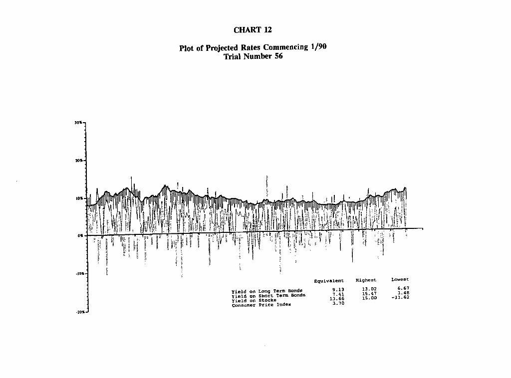
CHART 12
Plot of Projected Rates Commencing 1/90 Trial Number 56
30% -
-10%, -
-20% 1
' '.!i'i?li/'!!i/ :~ ~. ~,
I I ,
! * ~ ~ i " ~ ,~i~~!~ ~ i I
i ~ ~ i "
Equivalent
Y i e l d on Long Term Bonds 9.13 Yield on Short Term Bonds 7.41 Yield on Stocks 13.66 Consumer Price ~ndex 3.70
i! i .!
Highest Lowest
13.02 6.67 15.47 3.48 15.00 -11.62

CHART 13
Plot of Projected Rates Commencing 1/90 Trial Number 5
30~ -
20~ , ,
I 0 ~ .
O~
-10~,
-20~
,
Yield on Long Term Bonds Yield on Short Term Bonds Yield on Stocks Consumer Price Index
i Equivalent Highest Lowest
7.15 12.85 2.75 5.78 12.00 1.74
20.92 13.86 -11.63 2.07
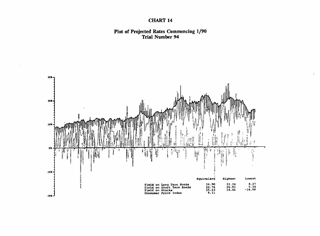
CHART 14
Plot of Projected Rates Commencing 1/90 Trial Number 94
"I
lOnG.
0~.
-~o~.t
-20 ~l, 1
~ ? I i:
Y i e l d on Long Term Bonds Y£e ld on Shoz't Term Bonds Y£e ld on S t o c k s Consumer Pr£ce Index
,~1 I" TV ili ;~
~. H~s.~ ~ . ~ ~ . ~ ~"
Equ£velen~ Highest Lowest 14.90 22.24 8.27 12.76 26.95 5.34 14.23 14.41 - 1 6 . 9 8
9 .11

CHART 15
Plot of Projected Rates Commencing 1/90 Trial Number 105
30%-
20%,
I I ~" ,,
• I
, | I, " i , . : . . ~
1 ,i I
I0%.
-I0%,
-20T
I
! ! n i , i ~ ~ ' '!'II'i r!l,JI,l:J JJl~,jJi rJll"J~,~lllJL Ji"P ~I' !JJ J"J i~i ~'~ l'J"
t i t ' , , ~ ~ ~ ~ , , , , :~ ~ ~ , , , ,
~iL ! ,! :~
Yield on Long Term Bonds Yield on Short Term Bonds Yield on Stocks Consumer Price Index
Equivalent Highest Lowest
7.03 8.26 4.00 5.96 12.36 2.68
10.29 15.85 -11.17 1.57
YIELD CURVE PROJECTION TECHNIQUES
Cookbook for History-Based Yield Curves, Etc.
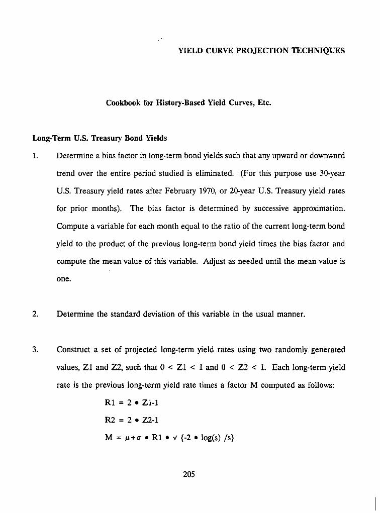
Long-Term U.S. Treasury Bond Yields
1. Determine a bias factor in long-term bond yields such that any upward or downward
trend over the entire period studied is eliminated. (For this purpose use 30-year
U.S. Treasury yield rates after February 1970, or 20-year U.S. Treasury yield rates
for prior months). The bias factor is determined by successive approximation.
Compute a variable for each month equal to the ratio of the current long-term bond
yield to the product of the previous long-term bond yield times the bias factor and
compute the mean value of this variable. Adjust as needed until the mean value is
one.
2. Determine the standard deviation of this variable in the usual manner.
. Construct a set of projected long-term yield rates using two randomly generated
values, Z1 and Z2, such that 0 < Z1 < 1 and 0 < Z2 < 1. Each long-term yield
rate is the previous 10ng-term yield rate times a factor M computed as follows:
R1 = 2 * ZI-1
R2 = 2 * Z2-1
M = ~ + a • R1 • "¢ {-2 * log(s) / s}
205
1990 SYMPOSIUM FOR THE VALUATION ACTUARY
Where s = R12 + R22,s < 1
If the value of s is equal to or greater than one, select new values of Z l and Z2.
Short-Term U.S. Treasury Bond Yields
1. Compute a variable equal to the absolute value of the difference between the long-
term bond yield over the short-term bond yield each month divided by the long-
term bond yield for such month. (For this purpose use 90-day Treasury bill rates
as short-term rates).
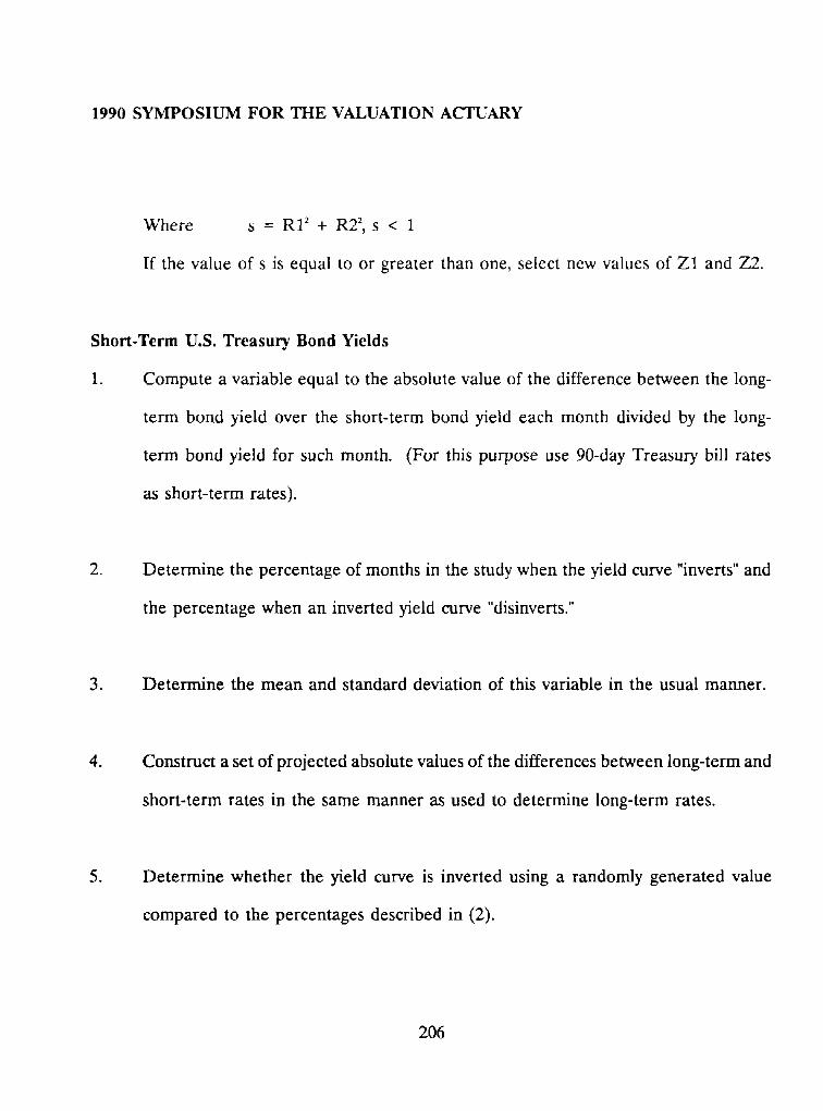
. Determine the percentage of months in the study when the yield curve "inverts" and
the percentage when an inverted yield curve "disinverts."
3. Determine the mean and standard deviation of this variable in the usual manner.
. Construct a set of projected absolute values of the differences between long-term and
short-term rates in the same manner as used to determine long-term rates.
. Determine whether the yield curve is inverted using a randomly generated value
compared to the percentages described in (2).
206
YIELD CURVE PROJECTION TECHNIQUES
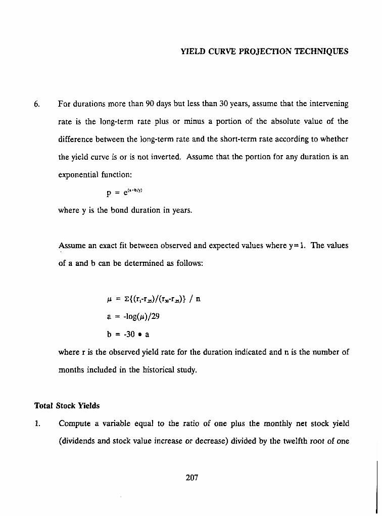
. For durations more than 90 days but less than 30 years, assume that the intervening
rate is the long-term rate plus or minus a portion of the absolute value of the
difference between the long-term rate and the short-term rate according to whether
the yield curve is or is not inverted. Assume that the portion for any duration is an
exponential function:
p = eC'+b/y)
where y is the bond duration in years.
Assume an exact fit between observed and expected values where y = 1. The values
of a and b can be determined as follows:
= ~.{(r,-r,~)/(rso-r,,)} / n
a = -log(/~)/29
b = -30 • a
where r is the observed yield rate for the duration indicated and n is the number of
months included in the historical study.
Total Stock Yields
1. Compute a variable equal to the ratio of one plus the monthly net stock yield
(dividends and stock value increase or decrease) divided by the twelfth root of one
207
1990 SYMPOSIUM FOR THE VALUATION ACTUARY
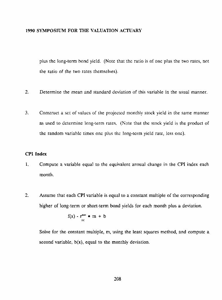
plus the long-term bond yield. (Note that the ratio is of one plus the two rates, not
the ratio of the two rates themselves).
2. Determine the mean and standard deviation of this variable in the usual manner.
. Construct a set of values of the projected monthly stock yield in the same manner
as used to determine long-term rates. (Note that the stock yield is the product of
the random variable times one plus the long-term yield rate, less one).
CPI Index
1. Compute a variable equal to the equivalent annual change in the CPI index each
month.
. Assume that each CPI variable is equal to a constant multiple of the corresponding
higher of long-term or short-term bond yields for each month plus a deviation.
f ( x ) - r ~ * m + b (x)
Solve for the constant multiple, m, using the least squares method, and compute a
second variable, b(x), equal to the monthly deviation.
208

YIELD CURVE PROJECTION TECHNIQUES
. Determine the mean and standard deviation of the second variable, b(x), in the usual
manner.
. Construct a set of values of projected equivalent annual changes in the CPI index
and the resulting CPI index for each month in the same manner used to determine
long-term rates.
For the seven prescribed scenarios (New York 126 and the proposed NAIC Model Act) fix
the long-term yields programmatically and compute the remaining rate according to the
"cookbook."
209

210
YIELD CURVE PROJECTION TECHNIQUES
MR. G R EG ORY D. JACOBS: As Tom mentioned, I 'm going to be talking about
something I guess I talked about awhile ago, and Tom affectionately called it the M&R
approach. I assume others have ~dopted it; it's too formal to call the M&R approach. It
is another approach to projecti',
Let's call it the yield-curve .
stochastic process.
", oroject future asset and liability cash flows.
': ' " , approach. It is, in fact, a
Let's start with some .!:,~
Yield curve one just ~
yield, curve, yield e. - ,.
much more robust t l i a ~ ,
yield curves of which we will p r o j e ' c , - ~ _
.eld curves in Chart 1.
~ five happens to be a high
;sent. In the real world, it's
• mple. This is the universe of
. ,se yield curves.
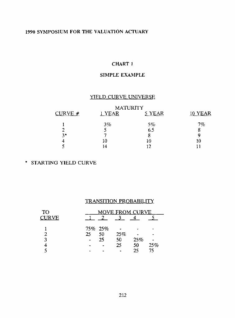
The next thing that we have to come up with using this particular approach is what we call
transition probability. Transition probability is a Markov chain, statistical sort of
211
1990 SYMPOSIUM FOR THE VALUATION ACTUARY
CHART 1
SIMPLE EXAMPLE
YIELD CURVE UNIVERSE
MATURITY CURVE # 1 YEAR 5 YEAR 10 YEAR
1 3 % 5 % 7 %
2 5 6.5 8 3" 7 8 9 4 10 10 10 5 14 12 11
" STARTING YIELD CURVE
TO CURVE
1
2 3 4 5
TRANSITION PROBABILITY
MOVE FROM CURVE 1 2 3 4 5
75% 25% 25 50 25% -
- 25 50 25% - - 2 5 5 0
- 2 5
25% 75
212
YIELD CURVE PROJECTION TECHNIQUES
terminology. It says if we are starting in some yield curve, we need to know the
probabilities to move from one to the other yield curve. Again in this very simplistic
example, Chart 1 shows that we started with yield curve three. We have a 50% chance of
staying in yield curve three for the next year-or the next period or the next quarter,
whatever it is we're projecting. We have a 25% chance of jumping to the top yield curve
or up one yield curve and a 25% chance of jumping down. When we get up into the
comers, it's a little interesting. This particular sort of example is probably not a good
example. It says once we get into the lowest yield curve or into the highest yield curve,
there's a high chance that we're going to stay. That's not very good when you see the real
one that I've developed. You'll see that it's a little bit different than that. But again, this
is just an illustration.
The mechanics are as follows. Let's pretend there's a four-sided die, because this is purely
a random number generator. We roll a four-sided die. If a "one" appears, we move from
curve three to two, a 25% chance. If a "two" or a "three" appears, we stay at curve three.
If a "four" appears we move up to curve four. That's what happens in.~ide the computer
model. If you have a transition probability that is not in 25% increments but is in 5%
increments, then you have a 20-sided die. Simple mechanics provide a very simple
computer routine to generate random numbers based on your transition probabilities to
move you through the various yield curves in each period. The magic is in what happens
213

1990 SYMPOSIUM FOR THE VALUATION ACTUARY
when the yield curve is set. This is universal to all systems that I've seen out there.
unique to M&R by any stretch of the imagination.
It's not
When a new yield curve is set, the interest-sensitive assumptions are triggered. We have
a new asset earnings rate, obviously, because now we have new investment rates of which
we're buying new assets at those new investment rates. We possibly have a new investment
strategy. Some companies set a different strategy when it's a high interest rate or inverted
yield curve or a variety of other issues, but we set a new investment strategy. Certainly the
market value has changed. Market values of all of our assets are driven by the Treasuries.
Calls and prepayments possibly occur depending on the specific formulas you have set up.
You probably have a new inflation rate, if your inflation rate is tied to some outside index.
Your credit rates probably are new because they're either going to be tied off of your
portfolio or some outside rate. Your market or competition rate is going to change,
presumably. Lapse rates will change because of the two above changes. When all is said
and done, new cash flows are computed. That is the entire yield curve projection process
and the results of those yield curve projections processes.
We do this for one period. At the end of the period, we throw the die again. We move
from the ending curve last period to the new curve this period; we go through all the
mechanics. We do that for x years, and we have a trial, 20 years, 30 years, whatever the
214

YIELD CURVE PROJECTION TECHNIQUES
case may be. Then we repeat the process. We go back to the starting yield curve, which
in our simple example yield curve is three. We set up some new random numbers, and we
go through the trials again. There's no "normal" number of trials. We often run 50 trials
because they fit on a page nicely. To be statistically significant, I believe it's been stated
in the past that you need at least 200 trials. I know that in some work we've done for
banks, we've literally done 2,000 trials to make them feel warm and fuzzy. They like
details. That's how the transition probability approach works.
The result of all of this stuff is that each move is independent of the previous move. I
personally believe that interest-rate movements this month have absolutely no dependence
on interest-rate movements last month or the month before. In this particular approach
every move is independent of the other move. Each move is also independent of the cash-
flow results of the company. All of these interest-rate projections are done before any cash
flows are computed. So, if you have positive cash flows or negative cash flows, they don't
influence at all what the yield curve is going to be next period. Each trial is totally
independent of the other trial except that the starting point is the same. The reason the
starting point is the same is because we have to start with today's yield curve or the
valuation date yield curve. This is classic Markov chain.
215
1990 SYMPOSIUM FOR THE VALUATION ACTUARY
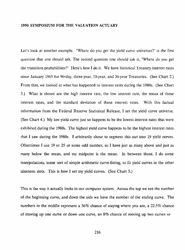
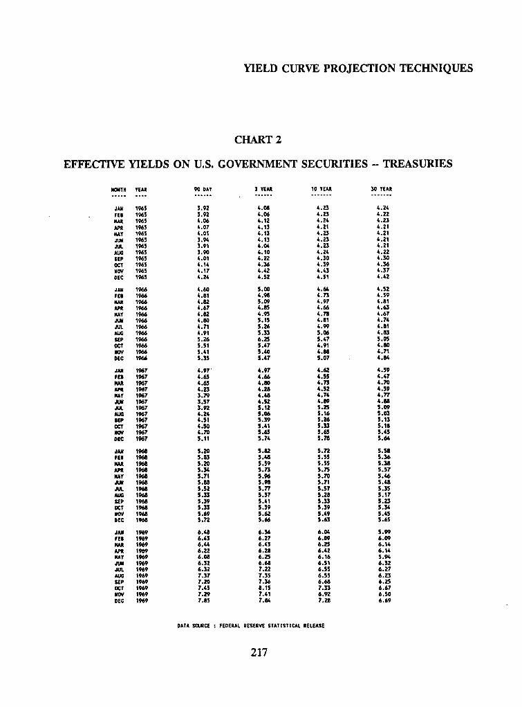
Let's look at another example. "Where do you get the yield curve universes?" is the first
question that one should ask. The second question one should ask is, "Where do you get
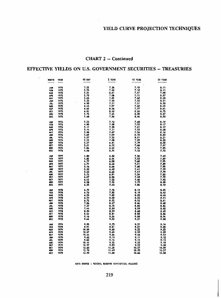
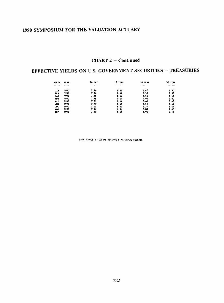
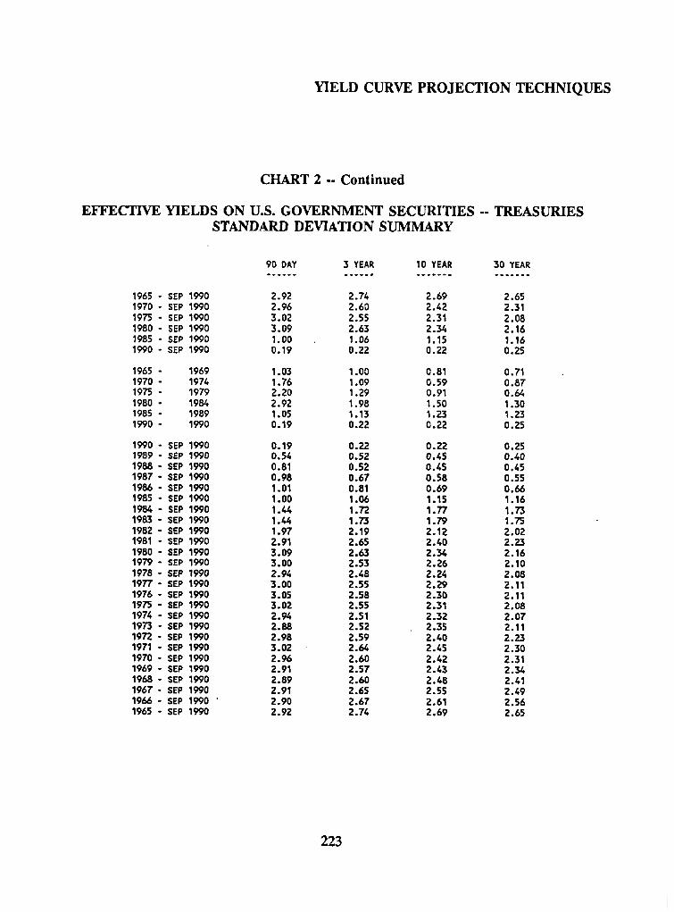
the transition probabilities?" Here's how I do it. We have historical Treasury interest rates
since January 1965 for 90-day, three-year, 10-year, and 30-year Treasuries. (See Chart 2.)
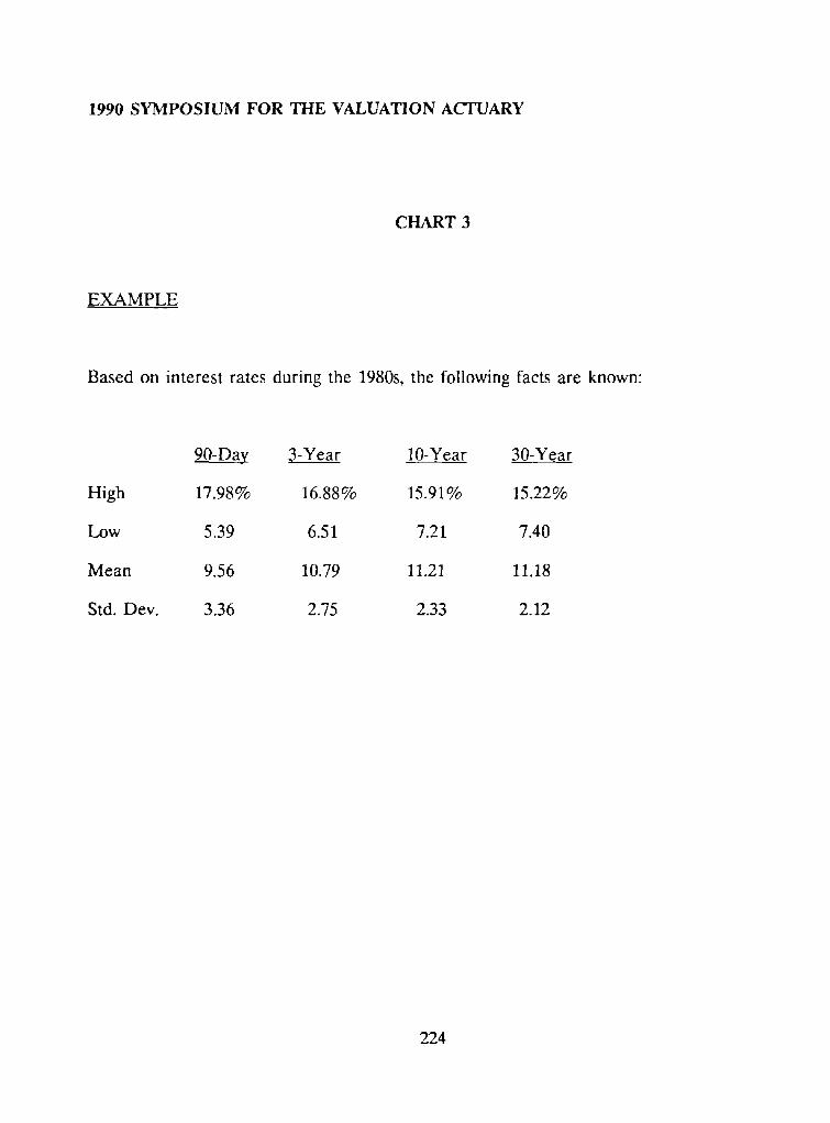
From that, we looked at what has happened to interest rates during the 1980s. (See Chart
3.) What is shown are the high interest rate, the low interest rate, the mean of those
interest rates, and the standard deviation of those interest rates. With this factual
information from the Federal Reserve Statistical Release, I set the yield curve universe.
(See Chart 4.) My low yield curve just so happens to be the lowest interest rates that were
exhibited during the 1980s. The highest yield curve happens to be the highest interest rates
that I saw during the 1980s. I arbitrarily chose to segment this out into 19 yield curves.
Oftentimes I use 19 or 25 or some odd number, so I have just as many above and just as
many below the mean, and my midpoint is the mean. In between those, I do some
interpolations, some sort of simple arithmetic curve-fitting, to fit yield curves in the other
nineteen slots. This is how I set my yield curves. (See Chart 5.)
This is the way it actually looks in our computer system. Across the top we see the number
of the beginning curve, and down the side we have the number of the ending curve. The
numbers in the middle represent a 36% chance of staying where you are, a 22.5% chance
of moving up one curve or down one curve, an 8% chance of moving up two curves or
216
YIELD CURVE PROJECTION TECHNIQUES
CHART 2
EFFECTIVE YIELDS ON U.S. GOVERNMENT SECURITIES - - TREASURIES
M~dTN YEAJt 90 DAY 5 YEAJt 10 YEAA 50 TEAR . . . . . . . . . . . . . . . . . . . . . . . . . . . . . . . . . . .
JAN 1965 5.92 4.08 &.~'~ 4.24 FEn 1965 3.92 4.06 4.23 4.22 ~l 1965 4.0(; 4.12 4.2/, 4.23 APR 1965 4.07 &.13 4.21 4.21 NAY 1965 4.01 &.13 4.23 4.21 JUN 1965 3.94 4.13 4.23 6.21
1965 3.91 4.04 &.Z3 4.21 AU¢ 3965 3.90 &.10 &.24 &.22 SEP 1965 &.01 4.22 &.30 4.30 OCT 1965 &.14 4.36 4.39 &.36 NOV 1965 4.17 4.42 4.43 4.37 DEC 1965 &.24 &.52 &.51 &.42
JAN 1966 4.60 5.00 4.6& 4.52 FED 1966 4.81 &.98 4.73 4.59 NAA 1966 4.82 5.09 t .97 4.81 APR 1966 4.67 &.85 4.66 & .63 KAY 1966 4.82 4.95 4.78 4.67
1966 4.80 5.15 4.81 4.7& JUt. 1966 4.71 5.26 4.99 4.81 AUG 1966 4.91 5.33 5.06 4.83 SEP 1966 5.26 6.25 5.&7 5.05
1966 5.51 5.&7 4.91 6.80 llOV 1966 5.41 5.40 6.88 4.71 8[C 1966 5.35 5.47 5.07 6.1K
1967 4.97' 6.97 4.62 4.59 FED 1967 4.65 &.66 &.55 4.47 NAA 1967 4.65 4.80 4.73 4.7'0 APt 1967 &.23 4.28 &.52 &.59 NAY 1967 3.79 4.&8 4.74 6.77 JUId 1967 3.57 &.52 4.89 4.88 JUt. 1967 3.92 5.12 5.25 5.09 AUa 1967 4.Z4 5.06 5.16 5.03 SEP 1967 &.51 5.39 5.26 5.13 OCT 1967 4.50 5.41 5.33 5.18
1967 &.70 5.65 5.65 5.45 DEC 1967 5.11 5.74 5.78 5.64
JAJI 1968 5.20 5.82 5.72 5.58 FEll 1968 5.03 5.&8 5.55 5.36 I~ t 1968 5.20 5.59 5.55 5 .M AJ~ 1968 5.34 5.73 5.73 5.57 NAY 19~ 5.71 5.96 5.?0 5.&6 JUil 1968 5.88 5.98 5.71 5 ./*8 JUt. 1968 5.52 5.77 5.57 5.35 AUG 1968 5.33 5.37 5.28 5.17 S£P 196~ 5.39 5.41 5.33 5.23 OCT 1968 5.33 5.39 5.39 5.34 NOV 1968 5.69 5.62 5.&9 5.45 DEC 1968 5.72 5.66 5.63 5.65
JAN 1969 6 . ~ 6.36 6.0& 5.99 FED 1969 6.43 6.27 6.09 6.09 PL~ 1969 6.~& 6.43 6.25 6.1& A.ntt 1969 6.22 6.28 6.&2 6.14 NAY 1969 6. ~5 6.25 6.16 5.9/, JUII 1969 6.32 6.68 6.51 6.32 JUL 1969 6.32 7.22 6.55 6.27 AUG 1969 7.37 7.35 6.55 6.23 S~P 1969 7.20 7.36 6.68 6.2.5 OCT t969 7.&5 8.15 7.33 6.67 NOV 1969 7.29 7.41 6.92 6.50 DEC 1969 7.85 7.86 7.28 6.69
DATA SOJR r'~ : FEDERAL RESERVE STATISTICAL rELEASE
217

1990 S Y M P O S I U M F O R THE V A L U A T I O N ACTUARY
CHART 2 -- Cont inued
E F F E C T I V E Y I E L D S O N U.S. G O V E R N M E N T S E C U R I T I E S -- T R E A S U R I E S
IqONTN Tr~l.J~ 90 DAY ] TF..AJI 10 YEAR 30 YEAR
JAR 197'0 8.37 8.39 7.54 6.91 FEB 19"/'0 8.25 8.33 7,64 6.94 MAR 197'0 7.14 7.30 6.94 6.50 APR 1970 6.62. 7,15 7,01 6.55 ~AY 1970 7.20 7.95 7.56 6.97 JU~ 1970 7.20 7.9~ 7.87 7.37
1970 6.34 7.92 7.70 7.15 AUG 1970 6.62 7.61 7.33 6.86 SEP 1970 6.50 7.40 7.49 6.9~ OCT 1970 5.99 7.0/* 7.24 6.7~ NOV 1970 6.03 6.91 7.32 6.92 DEC 1970 5.28 5.62 6.51 6.32
JAR 1971 4.97 5.78 6.&7 6.35 FEB 1971 4.22 5.30 6.08 6.G4
1971 3./,~ 4.86 6,10 6.20 APR 1971 3.66 4.48 5.56 5.66 HAY 1971 4.08 5.73 6.0~ 6.07
1971 4.41 5.86 6.30 6.22 ,RJt. 1971 5.22 6.52 6.50 6.40 AUG 1971 5.4.4 6.84 7.02 6.34 $EP 1971 4.40 5.85 6.33 6.01 OCT 1971 4.67 5.78 6.06 5.86 IIOV 1971 4.39 5.26 5.91 5.81 DEC 1971 4.42 5.36 6.04 5.87
JAN 1972 3.6,8 5.06 6.05 5.89 FEB 197'2 3.35 5.31 6.29 5.98 HAll 1972 3.49 5.33 6.27 5.94 APt 1972 3.87 5.83 6.30 6.02 NAY 1972 3.65 5.58 6.20 6.02
1972 3.86 5.41 6.18 3.86 ,KJI. 1972 3.99 5.70 6.21 5.91 AUG 1972 3.78 5.73 6.30 5.81 SEP 1972 4.60 6.01 6d,.6 5.77 OCT 1972 4.64 6.03 6.68 5.91 IIOV 197'2 4.86 6.O6 6.53 3.81 DEC 197'2 4.98 5.95 6.42 3.66
JAN 1973 5.27 6.04 6.43 5.91 FEB 1973 5.7'3 6.42 6.60 7.01 MAR 197'3 6.01 6.8?. 6.72 7.02 APR 1973 6.6?. 6.83 6.76 6.97 NAY 1973 6.42 6.79 6.76 7.00
1973 7.15 6.83 6.92 7.21 .KA, 1973 7.83 7.02 6.92 7.28 AUG 1973 8.70 8.04 7.35 7.7"2 SEP 1973 8.96 7.48 7.15 7.45 OCT 1973 7.24 6.86 6.92 7.13 I~V 1973 7.64 6.83 6.78 7.40 DEC 1973 7.57 6.B3 6.78 7.2 ]
JAN 1974 7.73 6.83 6.92 7.40 FEB 1974 7.79 6.91 7.0~ 7.53 MAJI 1974 7.7"5 6.9~ 7.00 7.62 APt 1974 0.69 7.90 7.23 7.95 NAY 1974 9.11 8.33 7.58 8.19
1974 0.44 8.17 7.56 0.23 • IUI. 1974 7.79 8.39 7.63 8.22 AUG 1974 8.27 8.76 7.85 8.58 SEP 1976 9.55 8.92 8.21 8.89 OCT 1974 6.38 8.17 7.64 0.63 NOV 1974 8.12 8.01 7.46 8.30 DEC 1974 7.74 7.50 7.7.3 8.18
DATA SOURCE : FEDERAL RESERVE STATISTICAL R£LEASE
218
YIELD CURVE P R O J E C T I O N T E C H N I Q U E S
CHART 2 -- Continued
EFFECTIVE YIELDS ON U.S. G O V E R N M E N T SECURITIES -- TREASURIES
NOIdTN YEAR 90 DAY 3 ¥EAN 10 YEAJt 30 YEAR
JAN 197'5 7.55 7.36 7.15 8.11 FEI 1975 5.93 7.02 7.12 8.11 NAR 1975 5.54 6.61 7.01 7.98 APt 1973 5.70 7.08 7.11 8.37 KAY 1975 5.63 7.85 7.62 8.58 J ~ 1973 5.33 7.30 7.52 8.51
1975 6.00 7.51 7.51 8.30 AUG 1975 6.43 7.97 7.62 8.&3 SEP 1975 6.65 8.06 7.77 8.61 OCT 1975 6.81 8.42 8.26 8.73 NOV 1975 5.7'3 7.24 8.00 8.37 0£0 1975 5.68 7.56 8.04 8.50
JAil 1976 5.33 7.12 7.68 8.19 FEll 1976 4.80 7.00 7.52 8.17 NAR 1976 5.11 7.20 7.61 8.17 APt 1976 5.14 7.11 7.52 8.08 NAY 1976 5.08 7.07 7.56 8 . I6
1976 5.69 7.59 8.10 8.33 JUL 19?6 5.57 7.33 8.01 8.21 AUG 1976 5.35 7.08 7.99 8.22 S~ 1976 5.27 6.81 7.79 8.05 OCT 1976 5.21 6.72 7.66 7.97 NOV 1976 5.04 6.42 7.54 7.95 0[0 1976 4.56 5.74 7.12 7.72
JAil 197'7 4.80 6.32 7.34 7.63 FER 1977 4.85 6.54 7.53 7.89 NAA 1977 6.77 6.58 7.60 7.95
1977 6.71 6.62 7.51 7.89 NAT 1977 5.16 6.66 7.60 7.95 ,KIN 1977 5.22 6.49 7.41 7.79 JUt. 1977 5.40 6.62 7.61 7.79 AUQ 1977 5.72 6.91 7.54 7.83 UP 1977 6.07 6.96 7.48 7.79 OCT 1977 6.45 7.32 7.66 7.92 J ~ 1977 6.M 7.35 7.72 8.00 DE r* 1977 6.35 7.43 7.84 8.10
JAN 1978 6.75 7.76 8.12 8.35 FEB 1978 6.76 7.82 8.19 8.62 NAR 19?8 6.59 7.85 8.20 8.40 APR 1978 6.59 8.00 8.32 8.51 NAY 1978 6.72 8.23 8.52 8.61 JUR 1978 7.06 8.47 8.64 8 .M JUt. 1978 7.37 8.72 8.83 8.84 AUG 1978 7. t,,4 8.50 8.59 8.65 SEP 19715 8.29 8.59 8.60 8.65 OCT 1978 8.4,4 8.81 8.83 8.86 NOV 1978 9.16 9.24 9.00 8.94 DEC 1978 9.64 9.55 9.21 9.M
JAN 1979 9.95 9.73 9.31 9.16 FEB 1979 9.91 9.51 9.31 9.20 NA, R 1979 10.09 9.60 9.33 9.Z3 APt 1979 10.07 9.65 9.39 9.29 NAY 1979 10.24 9.64 9.46 9.40
1979 9.62 9.15 9.11 9.12 JUL 1979 9.82 9.14 9.15 9.13 AUG 1979 10.14 9.35 9.23 9.18 SEP 1979 10.97 9.93 9.55 9.38 OCT 1979 12.60 11.25 10.57 10.09 NOV 1979 12.?0 11.49 10.93 10.57 OEC 19;'9 12.99 11.00 10.66 10.38
DATA SCURf[ : FEDERAL RESERVE STATISTICAL RELEASE
219

1990 SYMPOSIUM FOR THE VALUATION ACTUARY
CHART 2 - - Continued
EFFECTIVE YIELDS ON U.S. GOVERNMENT SECURITIES - - TREASURIES
NOMTR yEAR 99 OAT 3 YEAR 10 YEAR 30 YEAR
JAN 1990 12.94 11.18 11.09 10.8,8 FEO 1980 13.93 13.25 12.60 12.50 NAR 1980 16.67 14.34 13.16 12.TZ APR 1980 14.33 12.38 11.80 11.73 HAT 1980 9.09 9.66 10.44 10.63 JLA( 1980 7.43 9.12 10.02 10.03 JUt. 1980 8.52 9.49 10.51 10.50
1980 9.7'0 10.91 11.41 11.30 SEP 1980 10.98 11.91 11.84 11.66 OCT 1990 12.51 12.37 12.10 11.93 mOV 1900 14.94 13.73 13.08 12.73 DEC 1980 17.10 14.12 13.23 12.7"8
JAN 19~1 16.4~ 13.43 12.97 12.51 FED 1961 16.18 14.12 13.63 13.21 MAR 1981 14.51 13.97 13.55 13.09 APR 19~1 14.89 14.59 14.15 13.64 NAY 1981 17.98 15.65 14.60 14.06 JUN 1981 16.11 14.80 13.92 13.3~ JUt. 1981 16.37 15.7"2 14.79 14.05 AUG 1981 17.04 16.64 15.50 14.67 S£P 1981 16.08 16.88 15.91 15.21 OCT 1981 14.72 16.10 15.72 15.22 NOV 1981 11.6,5 13.54 ~3.&4 13.00 DEC 19151 11.63 14.13 14.19 13.90
JAN 1962 13.26 15.18 15.12 14.73 FEI 1982 14.65 15.27 14.95 14.7'3 14AJI 1982 13.72 14.63 14.34 13.99 APR 1982 13.75 14.88 14.35 13.82 MAT 1962 13.04 14.26 14.06 13.68 JUN 1962 13.48 15.00 14.81 14.40 JUI. 1982 12.20 14.49 14.&& 14.01 AUG 1982 9.20 13.02 13.49 13.18 $1EP 1982 8.36 12.39 12.72 12.43 OCT 1982 8.13 10.90 11.21 11.&8 NOV 1982 8.33 10.23 10.83 10.82 DEC 1982 8.38 10.12 10.82 10.02
JAN 1983 8.30 9.87 10.7'3 10.91 FEB 198.3 8.37 10.16 11.01 11.18 MAN 191L3 6.84 10.08 lO.T9 10.91 AP~ 19133 8.6~, 10.00 10.67 10.76 MAY 1983 6.66 9.89 10.65 10.81 JUN 1963 9.32 10.39 11.14 11.23 JUt. 19&3 9.64, 11.20 11.70 11.73 AUG 1983 9.93 11.62. 12.20 12.17 $1EP 1983 9.56 11.38 11.99 11.97 OCT 1983 9.16 11.17 11.87 11.92 NOV 1903 9.29 11.26 12.03 12.10 DEC 1983 9.56 11.44 12.18 12.23
JAN 1984 9. t~ 11.23 12.01 12.10 FEB 1984 9.66 11.36 12.19 12.31 MAN 191~ 10.1& 11.f3 12.70 12.76 API 1984 10.33 12.34 13.03 13.05 MAY 198/, 10J,8 13.16 13.&6 13.88 JUM 198~ 10.53 13.61 14.02 13.89 JUL 1984 10.81 13.51 13.01 13.65 AUG 1984 11.20 12.89 13.12 12,93 S1EP 1984 11.09 12.72 12.91 12.67 OCT 1984 10.38 12.20 12.53 12.3,; NOV 191~ 9.12 11.20 11.91 11.89 DEC 1984 8.52 10 .~ 11.63 11.85
DATA SG, J~CE : FEDERAL RESERVI~ STATISTICAL RELEASE
220

YIELD CURVE PROJECTION TECHNIQUES
CHART 2 -- Continued
EFFECTIVE YIELDS ON U.S. GOVERNMENT SECURITIES -- TREASURIES
14~TN YEAR 90 DAY 3 YEAR 10 YEAR 30 YEAR . . . . o . . . . . . . . . . . . . . . . . . . . . . . . . . . . . .
JAN 1985 8.19 10.70 11.70 11.78 FEB 1985 8.75 10.8.3 11.84 11.80 MAN 1985 9.02 11.36 12.21 12.16 APIt 1985 8.AO 10.77 11.76 11.80 KAY 1985 7,M 9.99 I I .1A 11.36 JiN 1985 7.30 9.26 10.&2 10.72 JUt. 1985 7.&& 9.39 10.58 10.78 AUG 1985 7.51 9.53 10.60 10.84 SEP 1985 7. t,,6 9.59 10.64 10.89 OCT 1985 7.53 9.4~ 10.50 10.78
19~,5 7.62 9.08 10.02 10.31 DEC 1985 7.&3 8.58 9.47 9.77
JAR 1986 7.&O 8.39 9.&O 9.62 F|I 1986 7.39 8.26 8.89 9.13
1986 6.91 7.&3 7.93 8.12 APl 19e6 6.34 6.98 7.&3 7.53 KAY 1986 6.40 7.40 7.86 7.66
1986 6.50 7.55 7.95 7.71 J~. 1986 6.10 6.98 7.43 7.40 AUG 1986 5.81 6.60 7.30 7.46 SEP 1986 5.40 6.73 7.59 7.77 OCT 1986 5.39 6.67 7.57 7.85 ~V 1986 5.57 6.56 7 .M 7.66 DEC 1986 5.72 6.53 7.24 7.51
1M7 5.M 6.51 7.21 7.53 FE8 1987 5.8.3 6.67 7.38 7 .M NUt 1967 5.80 6.69 7.38 7.69
19Q7 6.03 7.&5 8.18 8.62 KAY 1987 6.03 8.18 8.80 8.97 JU8 1987 5.95 7.97 8.58 8.75- JUL 1987 6.0~, 7.89 8.63 8.83 AUG 1967 6.29 8.19 8.95 9.17 S8P 1M7 6.64 8.86 9.64 9.82 OCT 1957 6.72 8.94 9.75 9.84 NOV 1967 6.09 8.15 9.06 9.15 DEC 1M7 6.07 8.30 9.19 9.33
JAN 1988 6.17 8.02 8.86 9.02 FEI 1988 5.95 7.52 8 .M 8.61 NAt 1988 5.95 7.64 8.55 8.82
19M 6.18 7.98 8.91 9.15 KAY 1988 6.55 8.61 9.30 9 . ~ JUN 1988 6.81 8.39 9.12 9.20 JUL 1988 7.06 8.62 9.27 9.35 AUG 1988 7.37 8.96 9./.7 9.54 SEP 1988 7.51 8.59 8.96 9 .M OCT 1988 7.62 8.35 8.73 8.86 NOV 1988 8.11 8.90 9.04 9.04 DEC 1968 8.34 9.15 9.19 9.02
JAN 1989 8.62 9.13 9.02 8.82 lEO 1989 8.96 9.&1 9 . ~ 9.13 lint 1989 9.25 9.72 9.36 9.16 APt 196'9 8.67 9.24 9.07 8.93 NAY 1989 8.92 8.81 8.66 8.62
1989 8.03 8.20 8.1/, 8.10 1989 7.98 7.77 7.97 8 .M
AUG 1989 7.90 8.37 8.25 8.20 SEP 1989 7.8/, 8.42 8.31 8.26 OCT 1989 7.60 7.86 7.89 7.91 llOV 1989 7.63 7.76 7.85 7.91 DEC 1989 7.68 7.90 7.93 7.98
DATA SOURCE : FEDERAL RES[RVE STATISTICAL RELEASE
221
1990 S Y M P O S I U M F O R T H E V A L U A T I O N ACTUARY
C H A R T 2 -- Cont inued
E F F E C T I V E Y I E L D S O N U.S. G O V E R N M E N T S E C U R I T I E S -- T R E A S U R I E S
NDNTH YEAR 90 DAY 3 TEAR 10 YEAR 30 YEAR
JAN 1990 7.76 8.38 8.4";' 8.50 FEI 1990 7,76 8.44 8.50 8,53
1990 7.85 8.57 8.$6 8.53 1990 7.78 9.01 9.02 9.00
~ I ' 1990 7.71 8.6/, 8.66 8.63 J'JM 1990 7.77 8.45 8.51 8.1,9 JUt. 1990 7.,f,3 8.12 8.37 8.~, AUG 1990 7.46 8.56 8.88 9.00 ~P 1990 7.29 8.58 8.96 9.10
DATA SOURCE : FEDERAL RESERV~ STAT|STIC, AL RELEASE
222
YIELD CURVE PROJECTION TECHNIQUES
CHART 2 - - Continued
EFFECTIVE YIELDS ON U.S. GOVERNMENT SECURITIES -- TREASURIES STANDARD DEVIATION SUMMARY
90 DAY 3 YEAR 10 YEAR 30 YEAR . . . . . . . . . . . . . . . . . . . . . . . . . .
1965 - SEP 1990 2.92 2.74 2 .69 2.65 1970 - SEP 1990 2 .96 2.60 2 .42 2.31 1975 - SEP 1990 3 .02 2.55 2.31 2 .08 1980 - SEP 1990 3 .09 2.63 2 .34 2 .16 1985 - SEP 1990 1.00 1.06 1.15 1.16 1990 - SEP 1990 0 .19 0.22 0 .22 0.25
1965 - 1969 1.03 1.00 0.81 0.71 1970 - 1974 1.76 1.09 0 .59 0 .87 1975 - 1979 2.20 1.29 0.91 0.64 1980 - 1984 2.92 1.98 1.50 1.30 1985 - 1989 1.05 1.13 1.23 1.23 1990 - 1990 0.19 0.22 0 .22 0.25
1990 - SEP 1990 0 .19 0.22 0 .22 0.25 1989 - SEP 1990 0.54 0.52 0 .45 0 .40 1988 - SEP 1990 0.81 0.52 0 .45 0.45 1987 - SEP 1990 0 .98 0 .67 0 .58 0.55 1986 - SEP 1990 1.01 0.81 0 .69 0 ,66 1985 - SEP 1990 1.00 1.06 1.15 1.16 1984 - SEP 1990 1.44 1.72 1 .77 1.73 1983 - SEP 1990 1.44 1.73 1 .79 1.75 1982 - SEP 1990 1.97 2 .19 2 .12 2 .02 1981 - SEP 1990 2.91 2.65 2 .40 2.23 1980 - SEP 1990 3 .09 2.63 2 .34 2 .16 1979 - SEP 1990 3 .00 2.53 2 .26 2 .10 1 9 7 8 - SEP 1990 2.94 2 .48 2 .24 2 .08 1977 - SEP 1990 3 .00 2.55 2 .29 2.11 1976 - SEP 1990 3.05 2 .58 2 .30 2.11 1975 - SEP 1990 3 .02 2.55 2.31 2 .08 1974 - SEP 1990 2.94 2.51 2 .32 2 .07 1973 - $EP 1990 2 .88 2.52 2 .35 2.11 1972 - SEP 1990 2 .98 2.59 2 .40 2.23 1971 - SEP 1990 3 .02 2.64 2 .45 2.30 1970 - SEP 1990 2 .96 2.60 2 .42 2.31 1969 - SEP 1990 2.91 2 .57 2 .43 2 .34 1968 - SEP 1990 2.89 2.60 2 .48 2.41 1967 - SEP 1990 2.91 2.65 2 .55 2 .49 1966 - SEP 1990 ' 2 .90 2 .67 2.61 2 .56 1965 - SEP 1990 2.92 2.74 2 .69 2.65
223
1990 SYMPOSIUM FOR THE VALUATION ACTUARY
CHART 3
EXAMPLE
Based on interest rates during the 1980s, the following facts are known:
90-Day 3-Year 10-Year 30-Year
High 17.98% 16.88% 15.91% 15.22%
Low 5.39 6.51 7.21 7.40
Mean 9.56 10.79 11.21 11.18
Std. Dev. 3.36 2.75 2.33 2.12
224

Y I E L D CURVE PROJECTION TECHNIQUES
CHART 4
EXAMPLE (CONTINUED)
SET YIELD CURVE UNIVERSE
CURVE # 90-Day 3-Year 10-Year 30-Year
Low 1 5.39% 6.15% 7.21% 7.40% 2 - -
3 - -
Mean 10 9.56 10.79 11.21 11.18
17 1 8 - -
H i g h 19 17.98 16.88 15.91 15.22 Today 20 7.37 8.96 9.47 9.54
Interpolate Interim Values
225
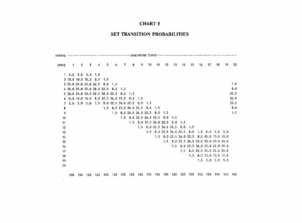
CHART 5
SET TRANSITION PROBABILITIES
ENDING . . . . . . . . . . . . . . . . . . . . . . . . . . . . . . . . . . . . . BEGINNING CURVE . . . . . . . . . . . . . . . . . . . . . . . . . . . . . . . . . . . . . . . . . . . . . . .
CURVE I 2 3 4 5 6 7 B 9 10 11 12 13 14 15 16 17 18 19 20
I
2
3
4
5
6
7
B
9
10
11
12
13
14
15
16
17
18
19
20
5.0 5.0 5.0 1.5 10.0 10.0 10.0 8.0 1.5
25.0 25.0 25.0 22.5 8.0 1.5 1.5
25.0 25.0 25.0 36.0 22.5 8.0 1.5 8.0
20.0 20.0 20.0 22.5 36.0 22.5 8.0 1.5 22.5
10.0 10.0 10.0 8.0 22.5 36.0 22.5 8.0 1.5 36.0
5.0 5.0 5.0 1.5 8.0 22.5 36.0 22.5 8.0 1.5 22.5
1,5 8.0 22.5 36.0 22.5 8.0 1.5 8.0
1.5 8.0 22.5 36.0 22.5 8.0 1.5 1.5
1.5 8.0 22.5 36.0 22.5 8.0 1.5
1,5 8.0 22.5 36.0 22.5 8.0 1.5
1.5 8.0 22.5 36.0 22.5 8.0 1.5
1.5 8.0 22.5 36.0 22.5 8.0 1.5 5.0 5.0 5.0
1,5 8.0 22.5 36.0 22.5 8.0 10.0 I0.0 10.0
1.5 8.0 22,5 36.0 22.5 20.0 20.0 20.0
1.5 8.0 22,5 36.0 25.0 25.0 25.0
1.5 8.0 22.5 25.0 25.0 25.0
1.5 8.0 10.0 10.0 10.0
1.5 5.0 5.0 5.0
100 100 100 100 100 100 100 100 100 100 100 100 100 100 100 100 100 100 100 100
YIELD CURVE PROJECTION TECHNIQUES
down two curves, and a 1.5% chance of moving up three curves or down three curves. Now
how did I get that? Simple math and an investigation of the interest rates during the 1980s.
This just happens to normally distributed. If we had looked at a different time period or
a different set of data, we probably wouldn't end up with a normal distribution. This
reproduces the standard deviation. What I have done in this simple example is to come up
with transition probabilities that replicate the standard deviations for the 1980s. I would
then take this to my client and expose its assets and liabilities to several random trials
through this process. I could then feel comfortable in determining whether or not I could
have withstood what happened during the 1980s. A different time period will definitely
yield different answers. There's no right answer in projecting yield curves. That's the bad
news, but the good news is, there's no wrong answer either. What I've tried to do with this
example through our particular approach, the yield-curve-universe transition-probability
approach, is to make use of historical data and use a Markov chain process to allow the
computer to conveniently project field curves.
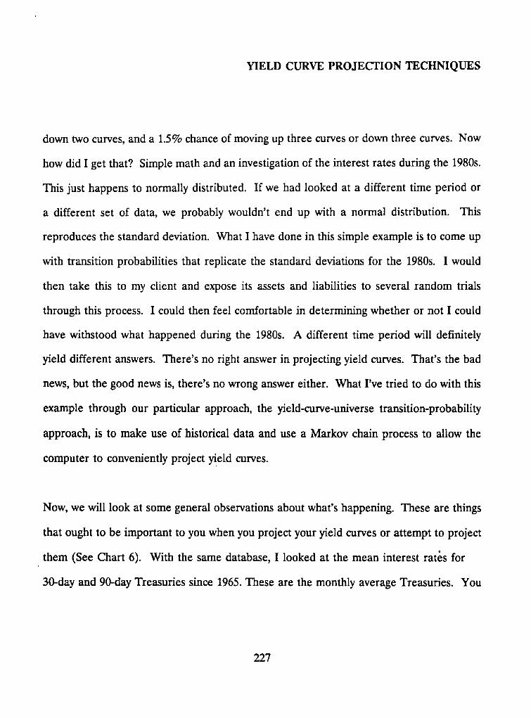
Now, we will look at some general observations about what's happening. These are things
that ought to be important to you when you project your yield curves or attempt to project
them (See Chart 6). With the same database, I looked at the mean interest rates for
30-day and 90-day Treasuries since 1965. These are the monthly average Treasuries. You
227
O9 ¢ ) ¢._
¢:
MEAN INTEREST RATES (30-YEAR AND 90-DAY TREASURIES)
,|
90 Day / ~ 18.0 15.0 14.0 13.0 12.0 11.0 10.0 9.0 8.0 7.0 8.0 5.0 4.0 3.0 2.0 1.0, 0.0
CHART 6
I I I I I I I I II I I I I I I I I I ! I I I I I i !
196519861967196819691970 1971 19721973 19"ill "19751978 1977 197819791980 1981 19821983 1984 19851986 1987 198819891990
Year

YIELD CURVE PROJECTION TECHNIQUES
will note a general increase from 1965 to the peak in 1981. There has been a general
decline since 1981. It now appears to be flattening out.
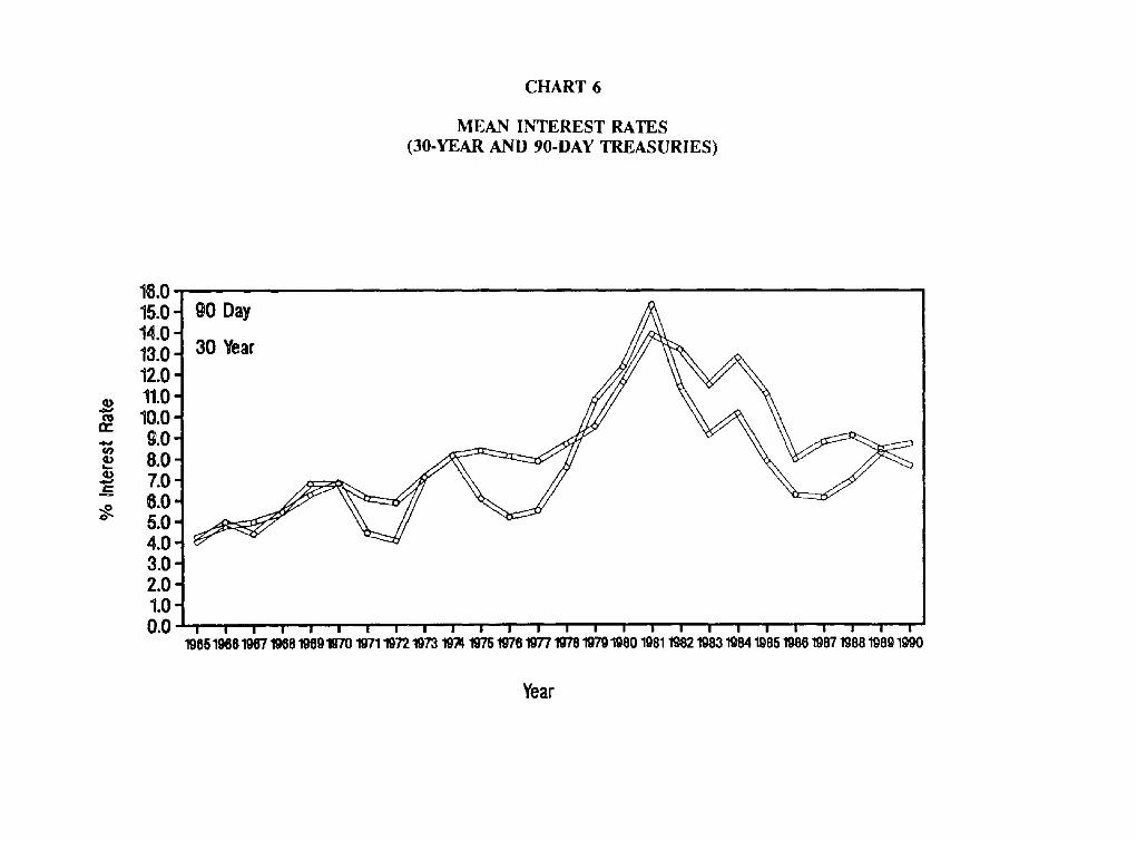
Chart 7 shows the number of inversions. I define an inversion as occurring when the 30-
year rate is less than the 90-day rate. Now, some approaches I have seen in yield curve
projections project an inordinate number of inversions, and I would submit to you that that's
because the data are couched in terms of early 1980, or prior, data. If you don't believe
that that's the real view of the world, then you ought to extract those and investigate your
yield curve projections pretty thoroughly because inversions have not been the norm since
1981. They've certainly been the exception.
Chart 8 is similar to the last one. It shows the yield curve slope again, just looking at the
30-year rate versus the 90-day rate. Several projection techniques that I have seen some
clients use is to project the slope that they put in a 90-day Treasury and one of the
variables is the slope. What I've gleamed from this is that's a terribly erratic assumption,
it's all over the place, and it's very difficult to be projecting what slopes are going forward
because it is so erratic. Again, I believe you need to investigate the results of any
projection technique you use to make sure that you have some reasonable numbers of slope.
You'll notice that since 1965 the slope has never gotten greater than about 1.58 and it's
229
CHART 7
NUMBER OF INVERSIONS (30-YR VS 90-DAY TREASURIES)
c 0 o0 L__
c
0
E
13 12 11 10 9 8 7 6 5 4 3 2 1 0 I I I I I I I " ' I i I l I I I I I I I I I I I I
198519081967 1968 19891970 1971 1972 197 ; 197q 1976197819771978197919801981 19821983 198419851986 1987 198819891990
Year
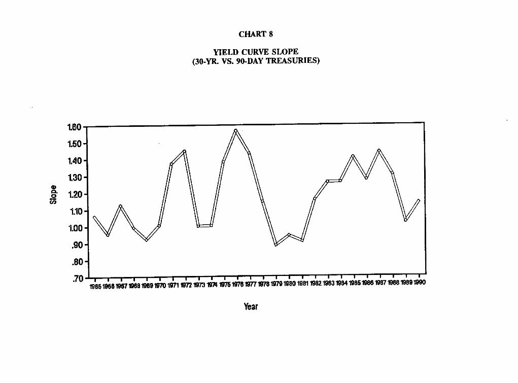
CHART 8
YIELD CURVE SLOPE (30-YR. VS. 90-DAY TREASURIES)
1.80 |
1.50 1 1.401 1.301
"90 t .80 .70-
196519861967196819691970 197119721973 19~ 197619761977197819791980 198119821983 198419851986 1987198819891990
Year
1990 SYMPOSIUM FOR THE VALUATION ACTUARY
never gotten lower than about .85. If you get some results that are
boundaries, something is a little awry with your projection.
outside those
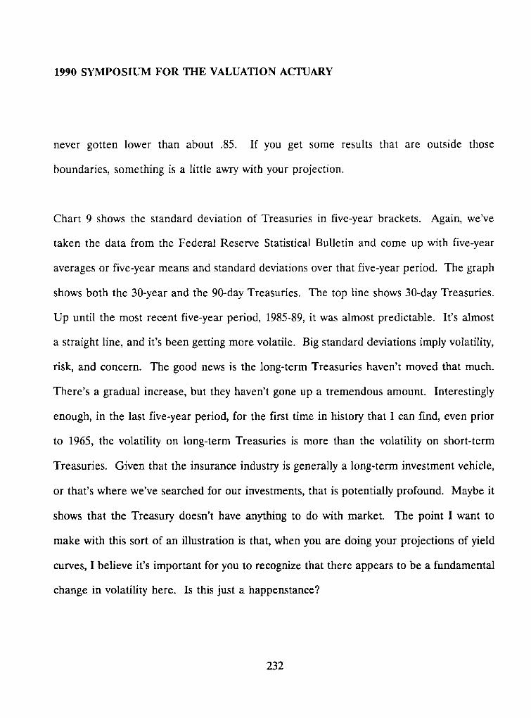
Chart 9 shows the standard deviation of Treasuries in five-year brackets. Again, we've
taken the data from the Federal Reserve Statistical Bulletin and come up with five-year
averages or five-year means and standard deviations over that five-year period. The graph
shows both the 30-year and the 90-day Treasuries. The top line shows 30-day Treasuries.
Up until the most recent five-year period, 1985-89, it was almost predictable. It's almost
a straight line, and it's been getting more volatile. Big standard deviations imply volatility,
risk, and concern. The good news is the long-term Treasuries haven't moved that much.
There's a gradual increase, but they haven't gone up a tremendous amount. Interestingly
enough, in the last five-year period, for the first time in history that I can find, even prior
to 1965, the volatility on long-term Treasuries is more than the volatility on short-term
Treasuries. Given that the insurance industry is generally a long-term investment vehicle,
or that's where we've searched for our investments, that is potentially profound. Maybe it
shows that the Treasury doesn't have anything to do with market. The point I want to
make with this sort of an illustration is that, when you are doing your projections of yield
curves, I believe it's important for you to recognize that there appears to be a fundamental
change in volatility here. Is this just a happenstance?
232
3.00 2.75"
i
2.50 - 2.25- 2,00
m ~
> 1.75 1°50 ,=~
1.25 '= 1.00
.75 .50
9{} 30
.25
.00
Day Treasury Ye
CHART 9
STANDARD DEVIATION OF TREASURIES (30-YEAR AND 90-DAY)
| i | i I
1965-1969 1970-1974 1975-1979 1980-1984 1955-1989
Years

1990 SYMPOSIUM FOR THE VALUATION ACTUARY
I don't know, but I've always structured my transition probabilities and my yield curve
universes with much more volatility in short-term rates than the long-term rates.
I want to leave you two things. One is that this is our approach, and there's not one
answer. Any number of M&R actuaries or any number of you with these same data could
probably set up different transition probabilities and different yield curve universes. This
is simply one approach. There are a lot of different approaches.
The second thing I would like to leave with you is something I've already said. There's
really no right answer. Projecting yield curves seems to have a fair amount of science
involved with it, but I am struck by the art that's involved much more than the science. If
you use this for anything other than a macro look at what happens to cash-flow testing, I
believe you are woefully out of line and putting way too much creditability in something
that is in fact a macro process as opposed to a micro process.
234

ARBITRAGE-FREE INTEREST RATE MODELS
MR. STEVEN P. MILLER: At the annual meeting of the Society of Actuaries, held in
Orlando in October 1990, there was a very well-attended workshop entitled "Interest Rate
Scenarios." Even though I was one of those many unfortunate members who registered too
late to be a confirmed attendee, I decided to be a gate-crasher. I justified my lawlessness
by telling myself that I needed to prepare for this panel. Apparently, I wasn't the only
person that felt a dire need to discuss this subject because there were 43 actuaries in a
room furnished to seat about 20. I think it was the second biggest attraction at the meeting.
The first had large, round ears.
One of the hottest topics of discussion in this workshop was the topic of arbitrage-free
interest rate scenarios, which incidentally, is the topic of my discussion. At the time, I
wasn't very sure about what I was going to say, so I took some notes about the questions
people were asking, and then built my presentation around those.
One question that wasn't asked, but that seems like a good place to start was, "What is
arbitrage, anyhow?" The usual definition of arbitrage is a risk-free profit that can be made
by simultaneously buying and selling identical items in different markets. The efficient
markets hypothesis of arbitrage pricing theory states that arbitrage cannot long exist because
235

1990 SYMPOSIUM FOR THE VALUATION ACTUARY
the buying and selling would soon drive prices to an equilibrium, where there was no profit
to be made. The strongest form of the hypothesis holds that the prices change so quickly
that arbitrage does not exist at all. Or, as a friend of mine is fond of saying, "No one can
create arbitrage, because everyone does."
I would like to point out, though, that the use of arbitrage-flee interest rate models does
require you to believe this hypothesis in its strongest form. In order to illustrate the value
of these models, I have created my own definition that I use when discussing interest rate
models: "Arbitrage is the state of affairs whereby a clever computer can create money out
of thin air." This definition points out the essence of arbitrage, (a profit without
investment) and the danger to proper modeling.
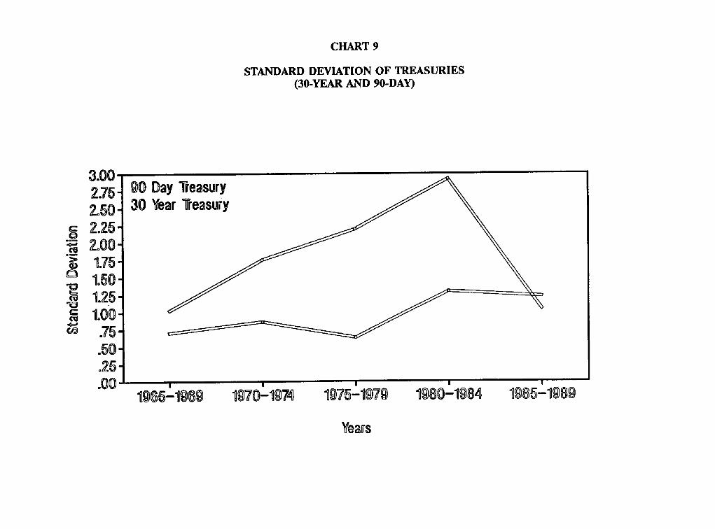
An interest rate model can contain arbitrage either because some points on the yield curve
are inconsistent with other parts of the same yield curve, or because the current yield curve
is inconsistent with the range of future yield curves. One example of a curve that is
inconsistent with itself is a yield curve that contains implicit negative spot prices (Chart 1).
Another is a curve that contains negative forward rates (Chart 2). The first allows arbitrage
because it allows a clever computer to receive positive cash flows in the future for a
negative "price." We can do this by buying the long bonds and selling a portfolio that
236
CHART 1
A YIELD CURVE WITH UNDEFINED SPOT RATES (From 20 years to 30 years)
12 .00%
03
C 0
O_
:::3 C ,c- 4:: c- O
O3
d ~ >-.
1 1 . 0 0
10 .00
9 .00
8 ,00
7 .00
6 .00 i i i i i 0 5 10 15 20 25 50
Maturiby
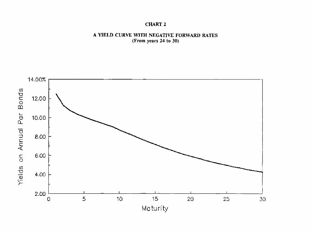
CHART 2
A YIELD CURVE WITH NEGATIVE FORWARD RATES (From years 24 to 30)
14.00%
03
c- O nq l _
O £1_
E] Z~ c- ( -
<
c- O
03
(1..) d - - >-
12.00
10,00
8,00
6,00
4.00
2,00 0
I
5 I I I
10 15 20
Maturity 25 30
YIELD CURVE PROJECTION TECHNIQUES
replicates the early coupons. The portfolio that we sold is more valuable than the bonds
that we bought, even though the long bonds pay all the cash that our shorter portfolio does,
and more. This type of arbitrage would only appear on models that projected yields on
coupon bonds, rather than spot rates . . . .
A second type of model arbitrage is probably more rare, only appearing in models that have
a low correlation between long and short rate changes. Chart 2 is an example of a yield
curve with negative implied forward rates. This creates arbitrage if we make the reasonable
assumption that cash pays 0% interest. By borrowing long and investing short, we can lock
in a future loan with a negative interest rate. Since we can hold the cash at 0%, we can
repay the loan by holding the sum of all payments and still have money left from the
proceeds of our loan. Once again, we have made money appear out of thin air.
The third type of arbitrage is the most common and also the hardest to understand. Here i
we will use the example of a typical yield curve (Chart 3). Like most real world problems,
I have created this curve from incomplete data. The unknown rates were created by linear
interpolation. Specifically, the curve is assumed to be linear between the five- and ten-
year maturities. I am going to assume that the yield curve six months from now is going
to be parallel to this one. In other words, if one rate goes up by 50 basis points, they all
do. Now I am going to test the investment strategy of selling seven-year bonds and buying
239

CHART 3
A TYPICAL YIELD CURVE
10%
J bJ
9,5
9
8,5
8
7,5
7 0
I I I
2 4 6
YEM~S TO MATURITY 8 10

YIELD CURVE PROJECTION TECHNIQUES
an equal amount of a barbell portfolio of five- and ten-year bonds. After six months, I am
going to sell my portfolio. According to my model, this strategy will allow me to make
money no matter what happens to interest rates (Chart 4). At the very minimum, I can
make .12% of the amount that I invested in seven-year bonds. While this doesn't sound
like much, remember that I didn't invest any of my own money. I imagine that anyone here
would love to have .12% of their company's money.
In this particular example (Chart 5), it is easy to see what is happening. First, as all three
securities age, they move down the yield curve. But the difference between the five (now
4.5) year and the rest of the bonds has increased by 2.5 basis points, allowing for a slight
capital gain relative to the other bonds. The duration of the barbell is equal to the
duration of the seven-year bullet, but the convexity is greater. This means that for small
changes in interest rates, the two portfolios move the same amount in relation to interest
rates, but for large changes, the barbell rises by more and falls by less.
Most models that actuaries would use would be more sophisticated than this one, but that
doesn't mean that arbitrage won't exist in these models. I have looked at some interest rate
models that seemed to be so complex that this couldn't possibly happen. Yet, by trial and
error, I have found portfolios that cost nothing, yet produced positive results over thousands
of scenarios.
241
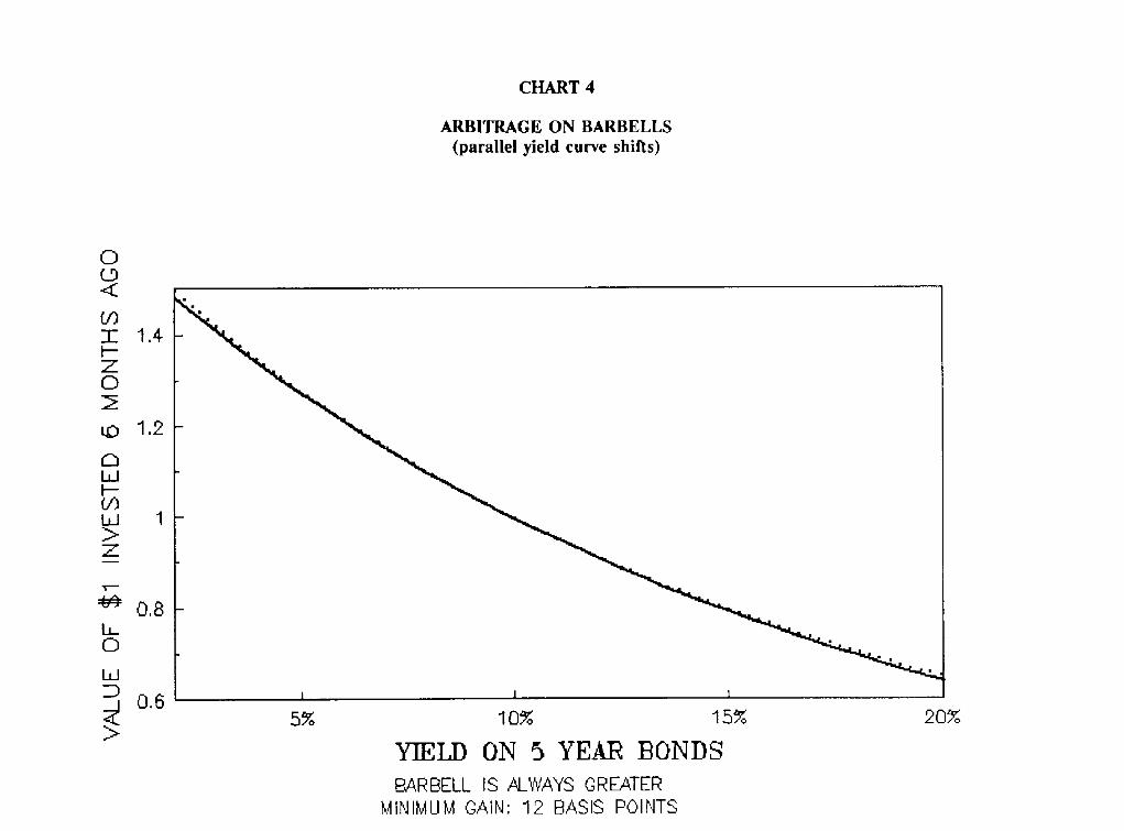
CHART 4
ARBITRAGE ON BARBELLS (parallel yield curve shifts)
0 (D <
GO I 1.4
Z 0
U3 1,2
E] W
O0 w I > Z
v. 0,8 I_1_ 0
W D 0,6 I I I
5% 10% 15%
"zq'i~,T.D ON 5 YEAR BONDS BARBELL IS ALWAYS GREATER
MINIMUM GAIN: 12 BASIS POll,ITS
20%
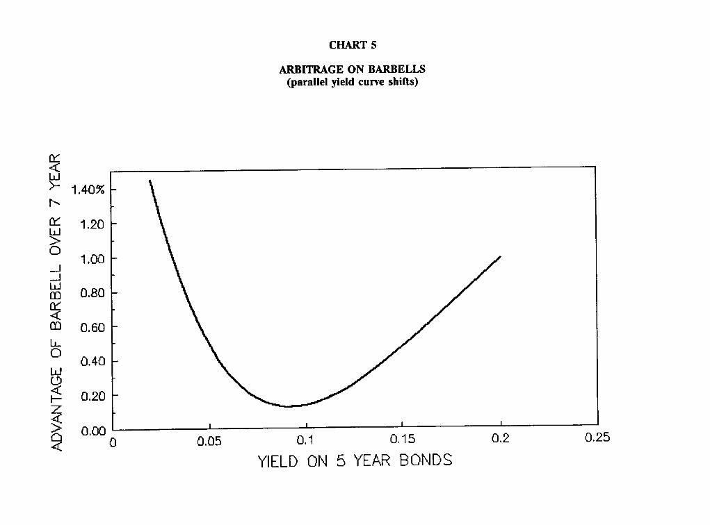
CHART 5
ARBITRAGE ON BARBELLS (parallel yield curve shifts)
< Ld
>-" 1.40% r-,,
1.20
1.00
d m w 0.80
m 0,60
~ 0.40
~ 0.20 Z
0.00
m
I I I I
E3 .< 0 0.05 0.1 0.15 0.2
YIELD ON 5 YEAR BONDS
0,25
1990 SYMPOSIUM FOR THE VALUATION ACTUARY
Now that we know what arbitrage is, it is an easy step to define an arbitrage-free model as
one that does not allow this to happen. It is not so easy to actually create one, which leads
to the first question: "Is it really necessary?"
This is an especially valid question since all of my examples have involved the buying and
selling of bonds, while most insurance companies tend to have a buy and hold strategy.
Since we don't plan on active trading, do we need to go through the trouble? The answer
is, "It depends." Remember that even if we don't short bonds or borrow money, we do
credit interest, which is very similar. If you were given the task of doing cash-flow testing
on a product where you were told that the credited rate is the portfolio rate, and that the
investment strategy was five-year bonds, I doubt that you would have problems. Your
computer wouldn't be clever enough since it is given both the crediting strategy and the
investment strategy. You may have a problem, though, if you found the results
unacceptable and were then told to find a better crediting or investment strategy. The
more talent you had toward solving that problem, the more likely you would be to find the
arbitrage in the model.
For example, in our parallel shift model, you may try a five- and ten-year barbell, instead
of a seven-year investment. This would give you at least a 12 basis point improvement, all
of which is attributable to arbitrage in the model, rather than to any real world economics.
244
YIELD CURVE PROJECTION TECHNIQUES
Worse, even though this difference is large enough to make a significant difference on a
leveraged product, it is probably too small to attract notice. It is very possible that this new
investment strategy would be hailed as a significant improvement, even if it wasn't. The
situation can get worse if you start to apply advanced optimization techniques in your
analysis, because then you have a very clever computer and are assured of finding arbitrage,
unless your constraints eliminate it.
The recent Exposure Draft entitled "Actuarial Standards of Practice -- Performing Cash
Flow Testing for Insurers" requires assumptions to be internally consistent. Arbitrage in an
interest rate model is an internal inconsistency. The current yield curve is inconsistent with
the assumed range of future yield curves. I think that an actuary ought to make certain
that this inconsistency does not distort his or her results. On the other hand, there are
many problems where the extra effort would not provide additional value, such as where
both the crediting strategy and investment strategy are simple and given in advance, and the
information sought is a range of possible results. In all circumstances, one should be on
the lookout for results that are biased by arbitrage. A good rule of thumb is that anything
that looks too good to be true, probably is.
Another question that is often asked is, What good is an arbitrage-free model? One answer
is that it helps an actuary avoid the types of errors that we are talking about. He is then
245
1990 SYMPOSIUM FOR THE VALUATION ACTUARY
free to worry about the thousands of other types of errors he might make.
arbitrage-free models are the essential ingredient of option pricing.
Another is that
It can be shown that, if there exists a probability distribution function where the expected
prices of bonds in the future are equal to the forward prices of those same bonds, then the
model is arbitrage free. Notice that I merely referred to the existence of such a
distribution. It is not necessary for this distribution to be used to generate random interest
scenarios. Arbitrage is a function of the range of possible future yield curves. It is not a
function of the probabilities of those curves. In a positive yield curve environment, most p
people would probably say that this "arbitrage distribution" is excessively biased toward
rising interest rates. However, there is one big advantage to calculating expected values
using this distribution.
Imagine that you are given a product where the cash flows are a function of future interest
rates. You would like to know how much it would cost to exactly fund that obligation. You
are going to have the perfect investment strategy so that no matter what path interest rates
take, you have exactly the amount of cash needed to fund the liability. No more, no less.
It can be shown that the amount of money needed to execute this strategy is equal to the
expected present value of the cash flows, where the expectations are taken using the
"arbitrage distribution" and the present values are calculated using the short-term rates
246

YIELD CURVE PROJECTION TECHNIQUES
along each interest rate path. Notice that in this perfect world, the actual probabilities are
irrelevant because the investment strategy works in every path, not just "on the average."
Since this is a valuation actuary symposium, we should answer the question, "What good is
option pricing to a valuation actuary?" The answer is that valuation is the perfect place to
use it. An option-based valuation can tell you whether you have enough assets to pay for
your obligations, what risk there is due to changes in interest rates, and what steps could
be taken to reduce that risk. The main disadvantage of an option-based valuation is the
large amount of effort and computer resources required to perform one. I personally
believe that this is a temporary problem and that both computer hardware and solution
methods will be improved to the point where option-based valuations are practical for a
large number of insurance companies.
An option-based valuation is similar to a market valuation in that it estimates the value of
an enterprise under current conditions. The values of both the assets and liabilities are
calculated using current interest rates and volatility assumptions. These values are normally
estimated by running random scenarios from an arbitrage free interest model, although
there are more efficient calculation methods for some types of securities. The difference
between the assets and the liabilities is the current surplus.
247

1990 SYMPOSIUM FOR THE VALUATION ACTUARY
It is also important to understand how sensitive the surplus is to interest rates. This can
be done by simply calculating the values with different starting yield curves. If you create
parallel shifts in your yield curves, and estimate the negative derivative of the natural
logarithm of the option value, with respect to the shift, then you have an option adjusted,
or effective, duration. You can calculate one measurement of convexity by taking the
second derivative of this quantity.
the liabilities, and for the surplus.
exposed to the risk of rising interest rates.
exposed to any changes in interest rates.
You can calculate these values for both the assets and
If the duration of the surplus is positive, then you are
If the convexity of surplus is negative, you are
If the durations are matched and the convexity
is positive, you are immunized against changes in the level of interest rates. Now you can
worry about different yield curve shifts.
One other question that was asked at the workshop was, How does one create an arbitrage-
free model? At first I decided not to tackle that one, because a panel discussion is a
difficult medium for that kind of information. Then I noticed that the program had
promised "Practical 'how-to' project yield curves," and since I haven't said anything practical
yet, I figured that I had better try. I am going to try to give a general description of how
to create a binomial lattice of interest rates, which is easy. The hard part is to make it
price the current yield curve.
248

YIELD CURVE PROJECTION TECHNIQUES
I like to think of a binomial lattice as more of a triangular matrix, than as a tree. As time
progresses, you go down one row per period. You can either go straight down, where
interest rates are lower, or down and to the right, where interest rates are higher. Now, let
me define some functions.
Binomial Lattice (Matrix Representation)
flslng Interest r ~ s
(o,o)
(1,0) (1,1)
(2,0)1 1 i(2,1) (3,0) (3,1) (3,2) (3,3)
(4,0) (4,1) (4,2) (4,3) (4,4)
249
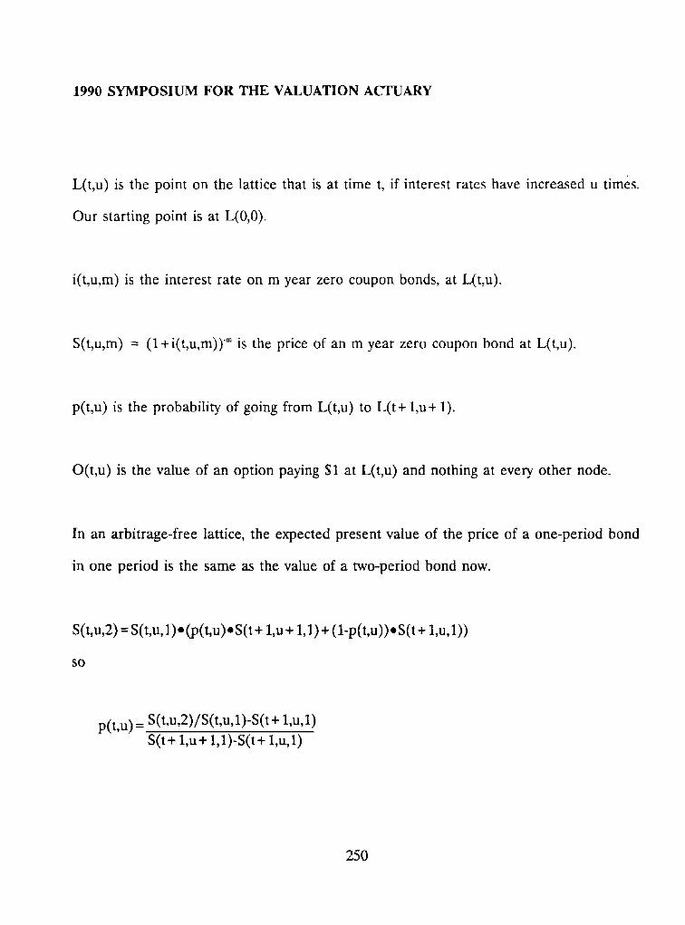
1990 SYMPOSIUM FOR THE VALUATION ACTUARY
L(t,u) is the point on the lattice that is at time t, if interest rates have increased u times.
Our starting point is at L(O,O).
i(t,u,m) is the interest rate on m year zero coupon bonds, at L(t,u).
S(t,u,m) = ( l+ i ( t ,u ,m))" is the price of an m year zero coupon bond at L(t,u).
p(t,u) is the probability of going from L(t,u) to L(t+ 1,u+ 1).
O(t,u) is the value of an option paying $1 at L(t,u) and nothing at every other node.
In an arbitrage-free lattice, the expected present value of the price of a one-period bond
in one period is the same as the value of a two-period bond now.
S(t,u,2) = S(t,u,1)-(p(t,u),.S(t + 1,u+ 1,1)+ (1-p(t,u)).S(t + 1,u,1))
s o
p(t,u) = S(t,u,2)/S(t,u,1)-S(t + 1,u,1)
S(t+ 1,u+ 1,1)-S(t + 1,u,1)
250
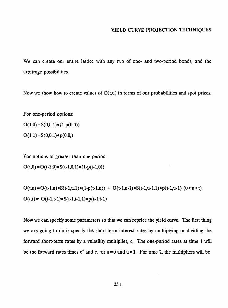
YIELD CURVE PROJECTION TECHNIQUES
We can create our entire lattice with any two of one- and two-period bonds, and the
arbitrage possibilities.
Now we show how to create values of O(t,u) in terms of our probabilities and spot prices.
For one-period options:
0(1,0) = S(O,O,1).(1-p(O,O))
0(1,1) = S(O,O,1)op(O,O,)
For options of greater than one period:
O(t,O) = O(t- 1,0). S(t-1,0,1).(1-p(t- 1,0))
O(t,u)=O(t-l,u).S(t-l,u,1).(1-p(t-l,u)) + O(t-l ,u-1).S(t- l ,u-l ,1) .p(t- l ,u-1)(0<u<t)
O(t,t) = O(t- l , t -1) ,S(t- l , t - l ,1)ep(t- l , t -1)
Now we can specify some parameters so that we can reprice the yield curve. The first thing
we are going to do is specify the short-term interest rates by multiplying or dividing the
forward short-term rates by a volatility multiplier, c. The one-period rates at time 1 will
be the forward rates times c 1 and c, for u = 0 and u = 1. For time 2, the multipliers will be
251
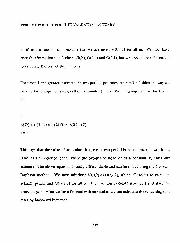
1990 SYMPOSIUM FOR THE VALUATION ACTUARY
c", c °, and c 2, and so on. Assume that we are given S(0,0,m) for all m. We now have
enough information to calculate p(0,0,), O(1,0) and O(1,1), but we need more information
to calculate the rest of the numbers.
For times 1 and greater, estimate the two-period spot rates in a similar fashion the way we
created the one-period rates, call our estimate r(t,u,2). We are going to solve for k such
that
t
X:{O(t,u)/(1 +ker(t,u,2)) ~} = S(O,O,t+2)
u = O
This says that the value of an option that gives a two-period bond at time t, is worth the
same as a t+2-period bond, where the two-period bond yields a constant, k, times our
estimate. The above equation is easily differentiable and can be solved using the Newton-
Raphson method. We now substitute i(t,u,2)=ker(t,u,2), which allows us to calculate
S(t,u,2), p(t,u), and O(t+ 1,u) for all u. Then we can calculate i(t+ 1,u,2) and start the
process again. After we have finished with our lattice, we can calculate the remaining spot
rates by backward induction.
252

YIELD CURVE PROJECTION TECHNIQUES
You probably noticed that there were many other ways that I could have forced my lattice
to price the curve, and I won't claim that this way is the best. I will say that I think it is
rather efficient, and has some other pleasing features. If the two-period volatility multiplier
is slightly less than the one-period multiplier, then the lattice will be mean-reverting. You
have to be careful, though, because if there is too much of a difference in the multipliers,
then the volatility of the long-term rates becomes very small.
This demonstration was not complete enough for you to go back and immediately build
an arbitrage-free interest rate model. You would have to go back to work and fill in some
holes, and I hope make some improvements. I do hope that I have given you some
guidance, and some insight into why I think it is worth the effort.
253

1990 SYMPOSIUM FOR THE VALUATION ACTUARY
Assumptions:
Spot Curve
Appendix A -- Numerica l E x a m p l e o f B inomia l Lattice
Maturity Yield 1 7.00% 2 7.50 3 7.75 4 7.90 5 8.00
Volatility Multiplier for 1-year rates Volatility Multiplier for 2-year rates
Step 1:
Calculate spot prices, S(O,O,m)
Maturity 1 2 3 4 5
Calculate forward rates
Years Forward
1 2 3 4
Y e a r s
Forward 1 2 3
= e .15 =
= e .l*s =
Price .935479 .865332 .799370 .737758 .680583
One-Year Price
.925905
.923772
.922924
.922501
Two-Year Price
.855326
.852572
.851398
1.161834 1.159513
One-Year Rate
8.0023% 8.2517 8.3251 8.4009
Two-Year Rate
8.1269% 8.3014 8.3760
254
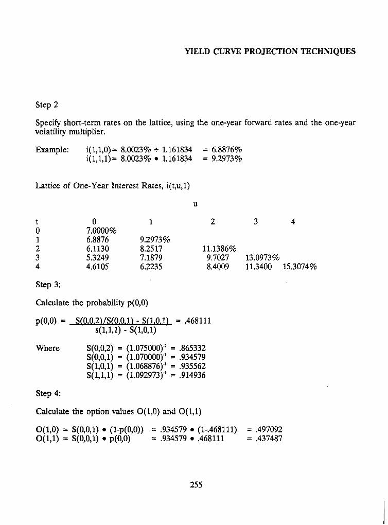
YIELD CURVE P R O J E C T I O N T E C H N I Q U E S
Step 2
Specify short- term rates on the lattice, using the one-year forward rates and the one-year volatility multiplier.
Example: i(1,1,0)= 8.0023% + 1.161834 = 6.8876% i(1,1,1)= 8.0023% • 1.161834 = 9.2973%
Latt ice of One-Year Interest Rates, i(t,u,1)
U
t 0 1 2 3 4 0 7.0000% 1 6.8876 9.2973% 2 6.1130 8.2517 11.1386% 3 5.3249 7.1879 9.7027 13.0973% 4 4.6105 6.2235 8.4009 11.3400 15.3074%
Step 3:
Calculate the probabil i ty p(0,0)
p(O,O) = S(0.0.2]/S(0.0.1) - S(1.0.D s ( i , l ,1 ) S(1,0,1)
S(0,0,2) = (1.075000)" S(0,0,1) = (1.070000) ~ S(1,0,1) = (!.068876) ~ S(1,1,1) = (1.092973) ~
Where
= .468111
= .865332 = .934579 = .935562 = .914936
Step 4:
Calculate the opt ion values O(1,0) and O(1,1)
O(1,0) -- S(0,0,1) • ( i -p(0,0)) = .934579 • (1-.468111) O(1,1) = S(0,0,1) • p(0,0) = .934579 • .468111
= .497092 = .437487
255

1990 SYMPOSIUM FOR THE VALUATION ACTUARY
Step 5:
Es t imate two-year rates r(1,0,2) and r(1,1,2) using two-year forward rates and two-year volatili ty multiplier.
r(1,0,2) = .081269 + 1.159513 = .070089 r(1,1,2) = .081269 • 1.159513 = .094232
Solve for k, in the equat ion
+ 0(1 ,1) = S(0,0,3) (1 + k•r(1,1,2)) 2
o(1,0) (1+ k•r(1,0,2)) ~
or
.497092 + .437487 = .799370 (1 + k• .070089) 2 (1 + k• .094232) '
using i terative techniques, k = 1.000985
i(1,0,2) = r(1,0 ,2)•k = .070089 • 1.000985 = .070158 i(1,1,2) = r (1 ,1 ,2)•k = .094232 • 1.000985 = .094325
Step 6:
Calcula te p(1,0) and p(1,1) using i(1,0,1), i(1,1,1), i(1,0,2), i(1,1,2), i(2,0,1), i(2,1,1), and i(2,2,1).
p(1,0) = .487124 p(1,1) = .462446
Step 7:
Calculate opt ion values 0(2,0) , 0(2,1) , and 0(2 ,2)
0(2,0) = o(1,o) = .497092
•s(1,0,1)•(1-p(1,0)) • .935562 • (1-.487124) = .238518
0(2 ,1) = 0(1 ,1) •S(1,1,1) . (1-p(1,1)) +0 (1 ,0 ) •S(1,O,1) •p(1,O) = .437487 • .914936•(1-.462446) +.497092 •.935562 •.487124 = .441710
256
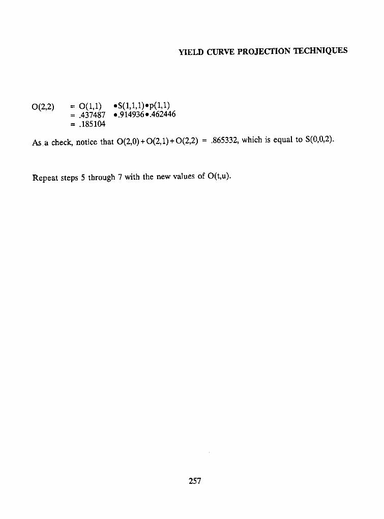
YIELD CURVE PROJECTION TECHNIQUES
0(2,2) = 0(1,1) = .437487 = .185104
.S(1,1,1).p(1,1) •.914936•.462446
As a check, notice that O(2,0)+O(2,1)+ 0(2,2) = .865332, which is equal to S(0,0,2).
Repeat steps 5 through 7 with the new values of O(t,u).
257

258