Overview of QM

( ) ( )n n nH E r r

ˆ ( , ) ( , )d

H t i tdt

r r

( , ) (0) ( )i tt e r r

( , ) ( ) ( )t t r r

ˆ( , ) ( ) ( , )t U t r r

2

ˆ ˆ ˆ ˆ ˆ( ) ( )2

H K V Vm

r r

Translational Motion2

ˆ ˆ ˆ2

Hm

Rotational Motion2

ˆ ˆ ˆ2

HI

L L

Vibrations

22ˆ ˆ ˆ ( )

2 2 eq

kH

r r

Cartesian

Spherical Polar

Centre of Mass

Statics

Dynamics

P. in Box

Rigid Rotor

Angular Mom.&Spin

Harmonic Motion

ex) STM, Devices

ex) FTS, NMR

ex) IR, Raman

Mol. dynamics, Q. Comp., Laser Pulse Methods,2D NMR, and SS NMR, andspectroscopy.

M.O. Calculations, Spectroscopy, andQ. Stat. Mech.

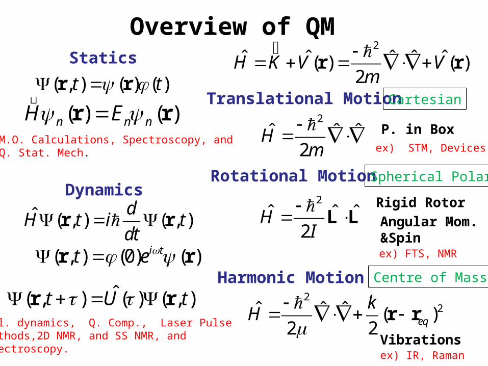
Quantum Mechanics for Many Particles

1 2 3 1 2 3( , , ,..., ) ( , , ,..., )n k n n kH E r r r r r r r r

2

,

ˆ ˆ ˆ ˆ ( , )2 i i ij i j

i i ji

H Vm

r r

1 2 3 1 2 3( , , ,..., , ) ( , ) ( , ) ( , )... ( , )k kt t t t t r r r r r r r r

( , ) ( ) ( )i i it t r r

1r

(0,0,0)

3r

2r4r

m1m3

m2m4

z1z3

z4z2

2

2ˆ ( , )

4

i jij i j i j

o i j

z z eV

r r r r

r r

En – Energy Levels n – Wavefuntions

Electronic Structure of Mols.

14_01fig_PChem.jpg

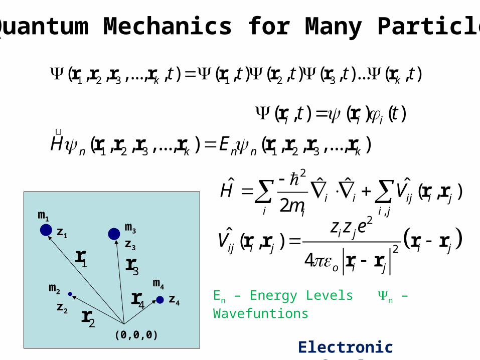
Properties of the Wavefunction

( , ) ( ) ( )x t x t Single Valued Finite and continuous

( ) (0) i tt e

2( , ) xx t d

2( , )x t

Im

Re

t

( )t

( , )x t

(0)o

ro

Complex Valued

14_01fig_PChem.jpg

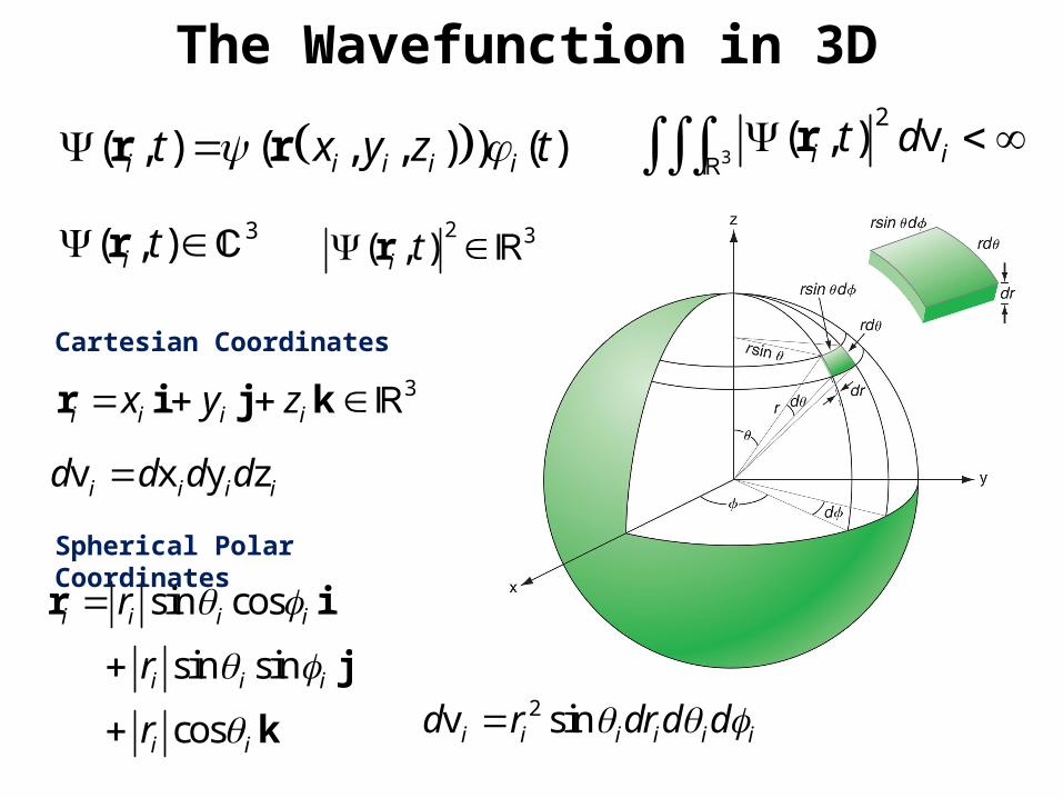
The Wavefunction in 3D

3i i i ix y z r i j k

3( , )i t r

sin cos

sin sin

cos

i i i i

i i i

i i

r

r

r

r i

j

k2v sin i i i i i id r drd d

( , ) ( , , ) ) ( )i i i i it x y z t r r 3

2( , ) vi it d r

v x y z i i i id d d d

Spherical Polar Coordinates

Cartesian Coordinates

2 3( , )i t r

Probability Distribution

2 *( , ) ( , ) ( , )t t t r r r

( , )t r *z z z z Recall

*( , ) ( , ) ( , )P t t t r r r Probability of finding the particle at exactly r, as a function of time.

*

( , ) ( , ) v ( , ) v

( , ) v

( , ) ( , ) v

j j j j

i i i i

x y z

x y z

R

R

P R t P t d P t d

P t d

t t d

r

r

r r

r

r r

Probability of finding the particle between ri and rj, defining the region R, as a function of time

Probability Distribution and Time

*( , ) ( , ) ( , ) vR

P R t t t d r r

*( ) ( ) ( ) ( ) v

R

t t d r r

* *

*

( ) ( ) ( ) v ( )

( ) ( ) ( )

R

t d t

t P R t

r r

*

*

( ) ( ) ( )

(0) (0) ( ) ( )i t i t

t t P R

e e P R P R

*( ) ( ) ( ) vR

P R d r r

Probability is independentof time!

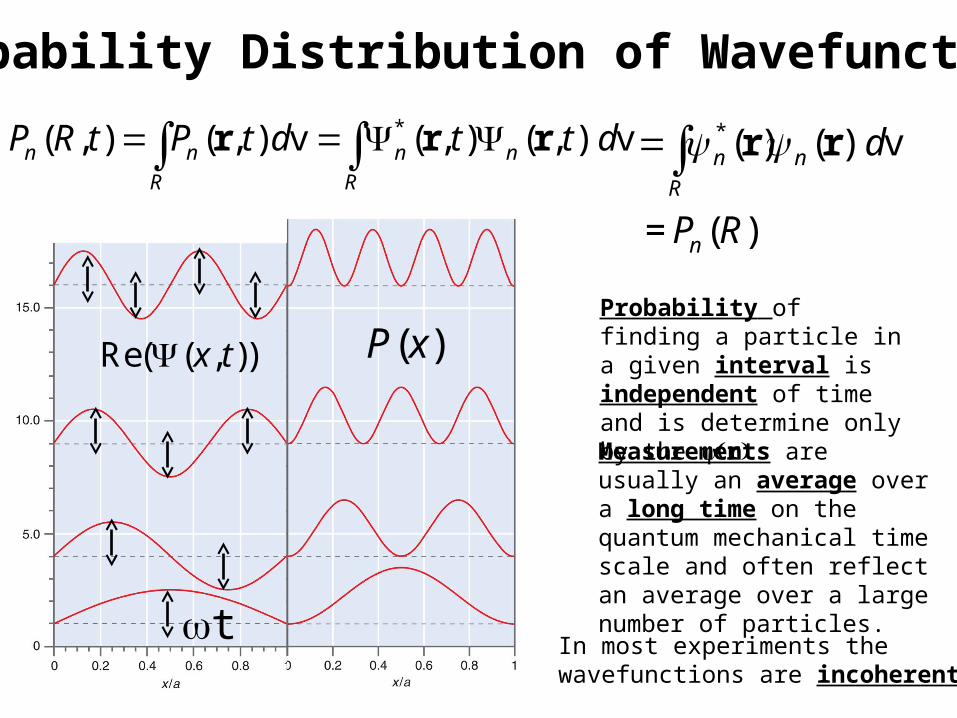
Probability Distribution of Wavefunctions*( , ) ( , ) v ( , ) ( , ) vn n n n

R R

P R t P t d t t d r r r *( ) ( ) v

= ( )

n n

R

n

d

P R

r r

Probability of finding a particle in a given interval is independent of time and is determine only by the r

Measurements are usually an average over a long time on the quantum mechanical time scale and often reflect an average over a large number of particles.

t

Re( ( , ))x t ( )P x

In most experiments the wavefunctions are incoherent.

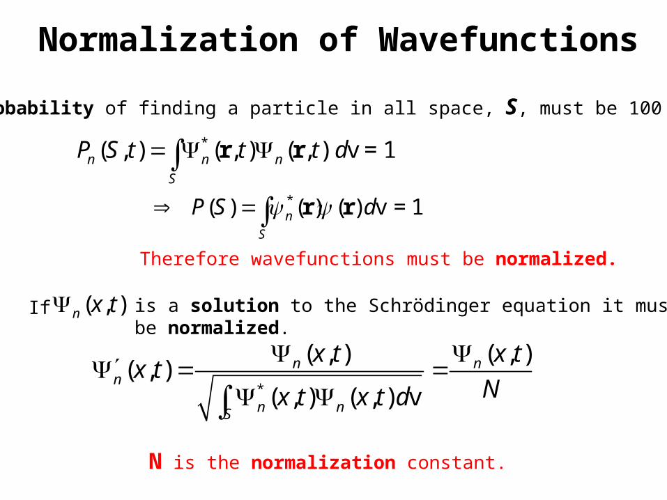
Normalization of Wavefunctions

*( ) ( ) ( ) v = 1n

S

P S d r r

The probability of finding a particle in all space, S, must be 100 %.

*( , ) ( , ) ( , ) v = 1n n n

S

P S t t t d r r

Therefore wavefunctions must be normalized.

( , )n x tIf is a solution to the Schrödinger equation it must be normalized.

*

( , ) ( , )( , )

( , ) ( , ) v

n nn

n nS

x t x tx t

Nx t x t d

N is the normalization constant.

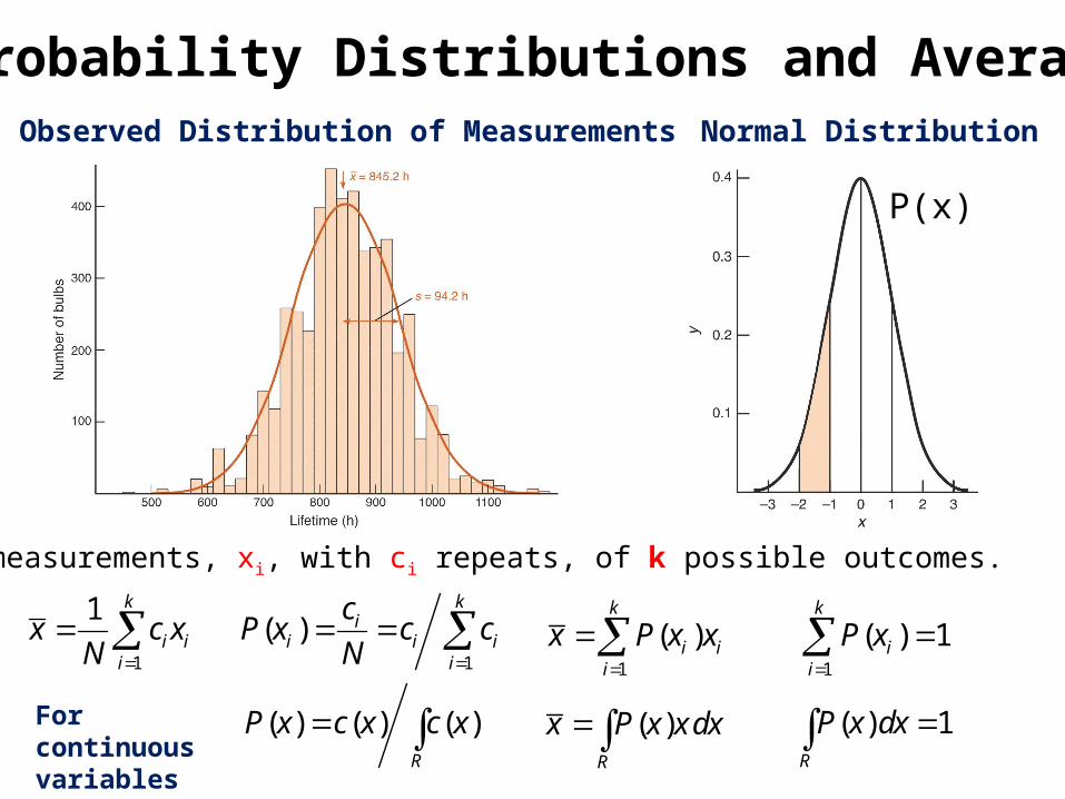
Probability Distributions and AveragesObserved Distribution of Measurements Normal Distribution

N measurements, xi, with ci repeats, of k possible outcomes.

1

1 k

i ii

x c xN

1

( )k

ii i i

i

cP x c c

N

1

( )k

i ii

x P x x

1

( ) 1k

ii

P x

( ) ( ) ( )R

P x c x c x ( )R

x P x xdx ( ) 1R

P x dx

P(x)

For continuous variables

Expectation Values

( )n

R

x P x xdx * *( , ) ( , )n n

R

x t x t xdx

*( ) ( )n n

R

x x x dx * ˆ( ) ( )n n

R

x x x dx x * ˆ( ) ( )n n

R

O x O x dx

Measurements are averages in time and large number of particles of observables.

Every observable has a corresponding operator

Expectation value of x.

*( ) ( ) ( ) ( )n n n n

R

x t x t xdx * *( ) ( ) ( ) ( )n n n n

R

x x x dx t t

*( ) ( ) 1n nt t

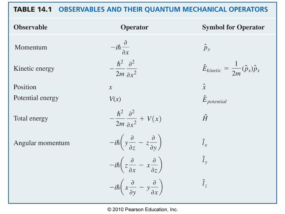
14_01tbl_PChem.jpg

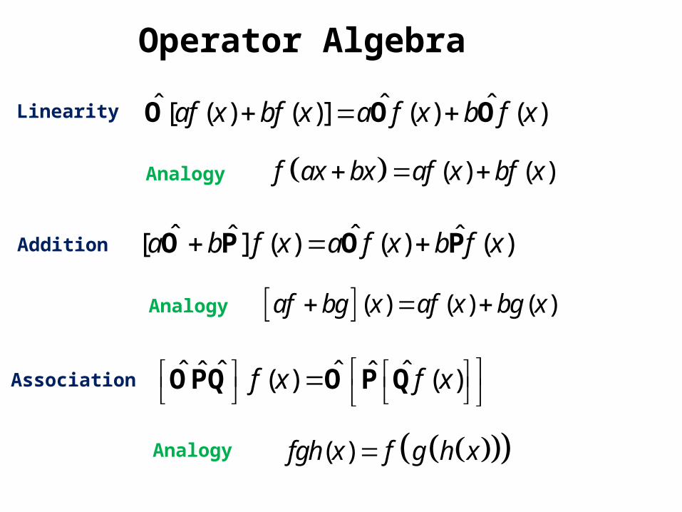
Operator Algebra

ˆ ˆ ˆ[ ( ) ( )] ( ) ( )af x bf x a f x b f x O O O

ˆ ˆˆ ˆ[ ] ( ) ( ) ( )a b f x a f x b f x O P O P

Linearity

Addition

Association ˆ ˆ ˆ ˆˆ ˆ( ) ( )f x f x OPQ O P Q

( ) ( )f ax bx af x bf x Analogy

( ) ( ) ( )af bg x af x bg x Analogy

( )fgh x f g h xAnalogy

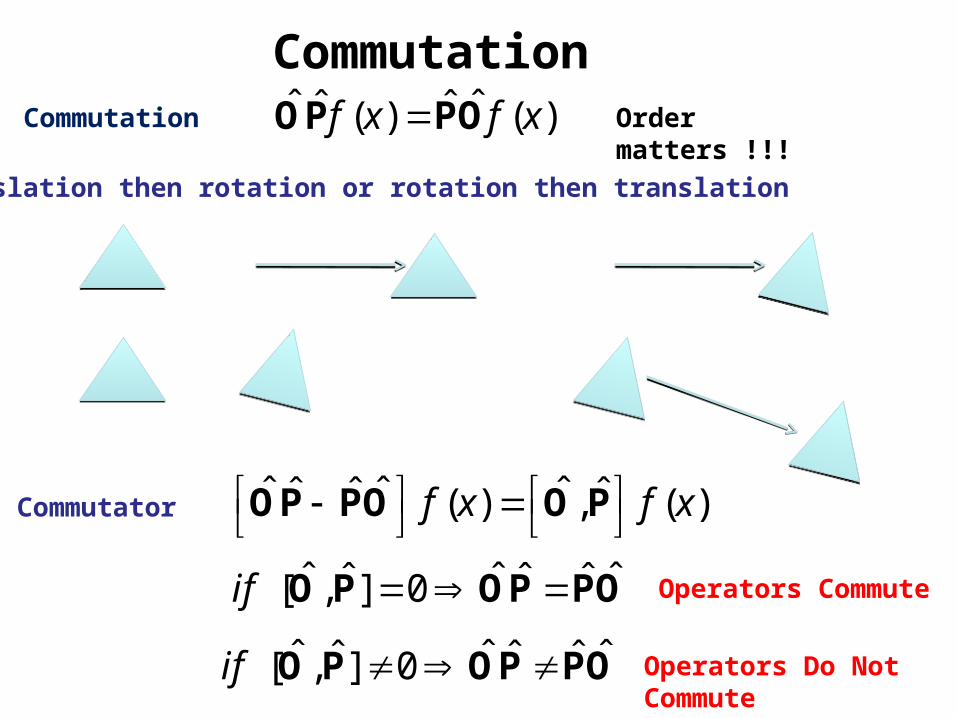
Commutation ˆ ˆˆ ˆ( ) ( )f x f xOP PO

ˆ ˆ ˆˆ ˆ ˆ( ) , ( )f x f x OP PO O PCommutator

ˆ ˆ ˆˆ ˆ ˆ[ , ] 0if O P OP PO

Order matters !!!

Operators Commute

ˆ ˆ ˆˆ ˆ ˆ[ , ] 0if O P OP PO Operators Do Not Commute

Translation then rotation or rotation then translation

Commutation

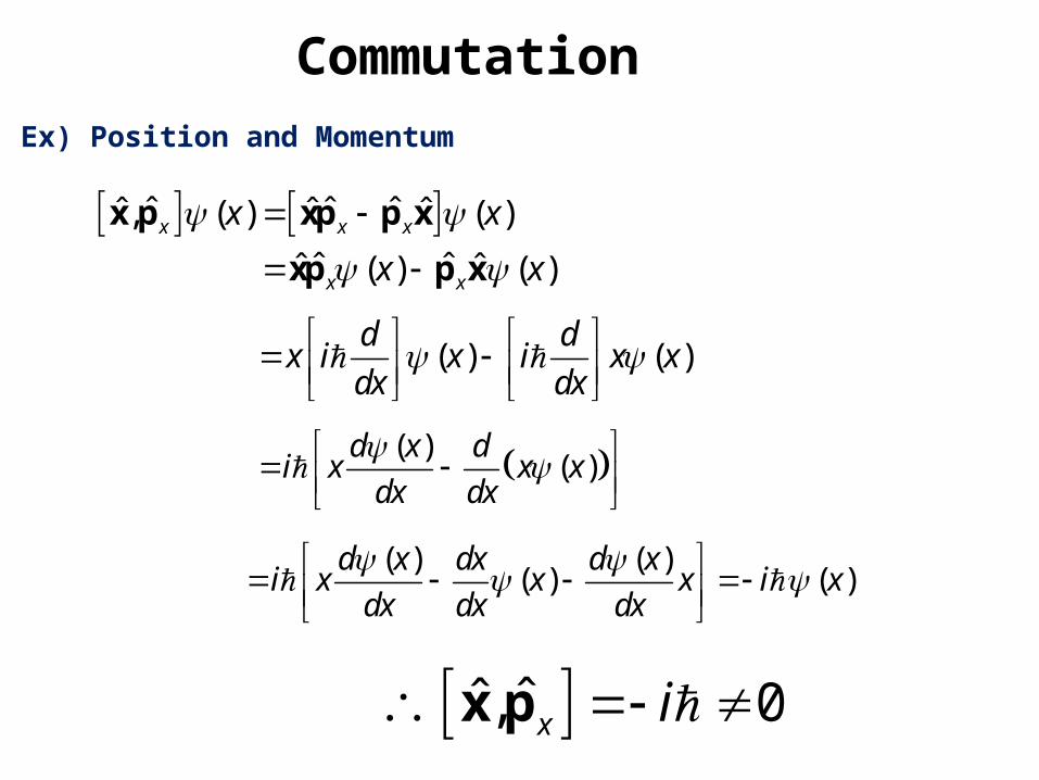
CommutationEx) Position and Momentum

ˆ ˆ ˆˆ ˆ ˆ, ( ) ( )

ˆ ˆˆ ˆ( ) ( )x x x

x x

x x

x x

x p xp p x

xp p x

( ) ( )d d

x i x i x xdx dx

( )( )

d x di x x x

dx dx

( ) ( )( ) ( )

d x dx d xi x x x i x

dx dx dx

ˆˆ , 0x i x p

Properties of Hermitian Operators

*ˆ ˆA AT

ˆ ( ) ( )n n nx a x A

* *( ) ( ) ( ) ( )n n n n n n

n

x a x dx a x x dx

a

* * * * * *

*

ˆ( ) ( ) ( ) ( ) ( ) ( )n n n n n n n n

n

x x dx x a x dx a x x dx

a

A

*n n na a a

* ˆ( ) ( )n nx x dx A

RHS

For matrices

* * *ˆ ˆ( ) ( ) ( ) ( )S S

x x dx x x dx A A

For functions

* * * *ˆ ( ) ( )n n nx a x A

LHS

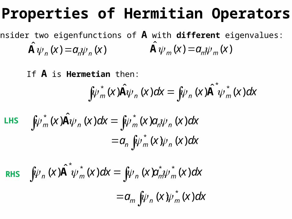
ˆ ( ) ( )n n nx a x A

Properties of Hermitian Operators

ˆ ( ) ( )m m mx a x A

** *ˆ ˆ( ) ( ) ( ) ( )m n n mx x dx x x dx A A

* * * *ˆ( ) ( ) ( ) ( )n m n m mx x dx x a x dx A

*( ) ( )m n ma x x dx

* *ˆ( ) ( ) ( ) ( )m n m n nx x dx x a x dx A

Consider two eigenfunctions of A with different eigenvalues:

If A is Hermetian then:

* ( ) ( )n m na x x dx

RHS

LHS

Properties of Hermitian Operators

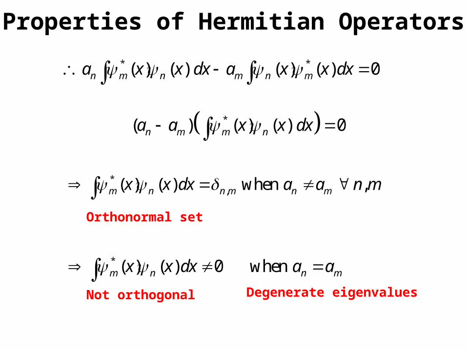
* *( ) ( ) ( ) ( ) 0n m n m n ma x x dx a x x dx

*( ) ( ) ( ) 0n m m na a x x dx

*,( ) ( ) when ,m n n m n mx x dx a a n m

* ( ) ( ) 0 whenm n n mx x dx a a

Orthonormal set

Degenerate eigenvaluesNot orthogonal

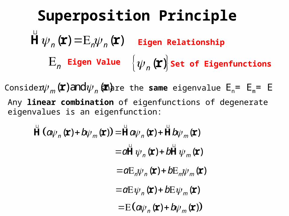
Superposition Principle

( ) ( )n n n H r r

( )n r

Eigen Relationship

n Eigen Value Set of Eigenfunctions

Any linear combination of eigenfunctions of degenerate eigenvalues is an eigenfunction:

( ) ( ) ( ) ( )n m n ma b a b H r r H r H r

( ) ( )n ma b H r H r

Consider ( ) and ( )m n r r share the same eigenvalue En= Em= E

( ) ( )n n m ma b r r

( ) ( )n ma b r r

( ) ( )n ma b r r

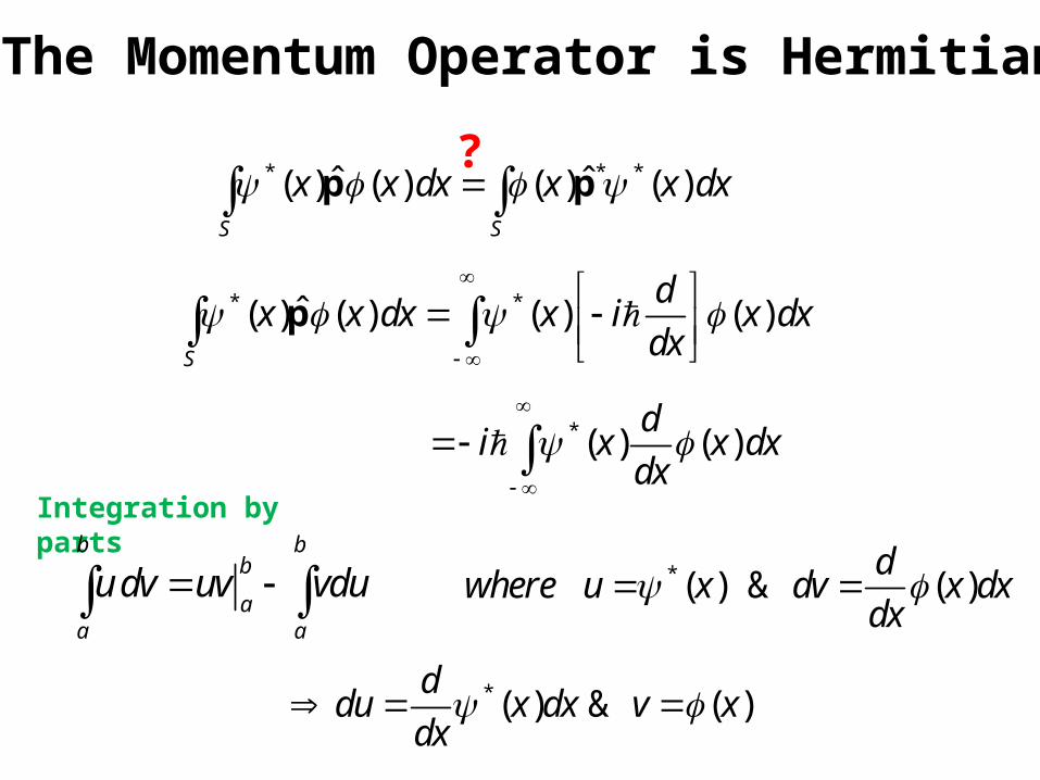
The Momentum Operator is Hermitian

* * *ˆ ˆ( ) ( ) ( ) ( )S S

x x dx x x dx p p

* *ˆ( ) ( ) ( ) ( )S

dx x dx x i x dx

dx

p

Integration by parts

?

b bb

aa a

udv uv vdu

*( ) ( )d

i x x dxdx

*( ) & ( )d

du x dx v xdx

*( ) & ( )d

where u x dv x dxdx

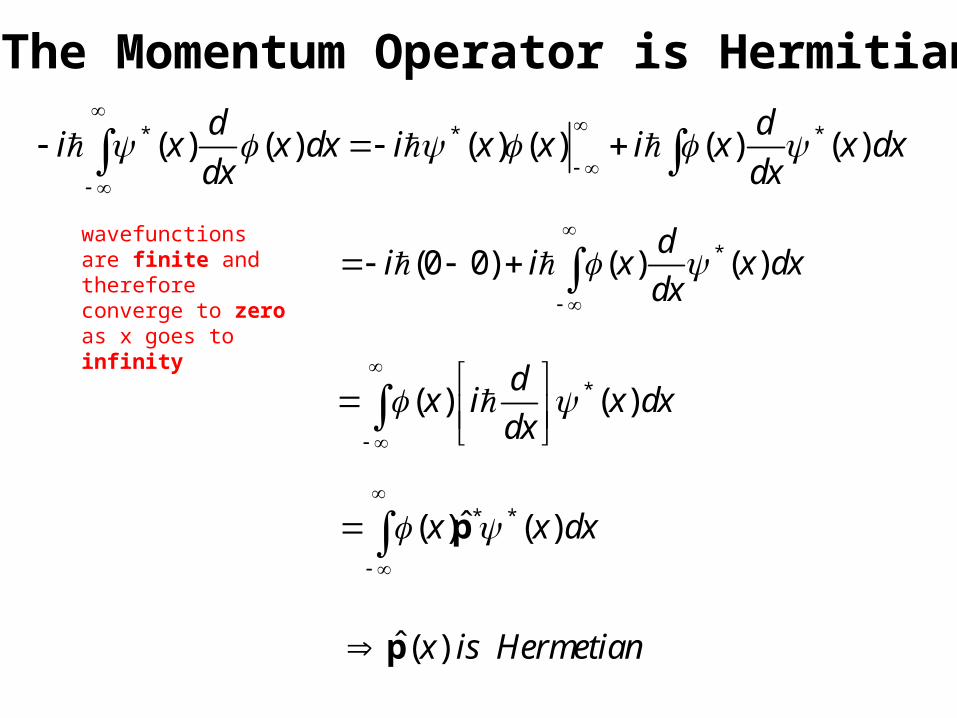
The Momentum Operator is Hermitian

* * *( ) ( ) ( ) ( ) ( ) ( )d d

i x x dx i x x i x x dxdx dx

wavefunctions are finite and therefore converge to zero as x goes to infinity

*(0 0) ( ) ( )d

i i x x dxdx

*( ) ( )d

x i x dxdx

* *ˆ( ) ( )x x dx

p

ˆ ( )x is Hermetian p

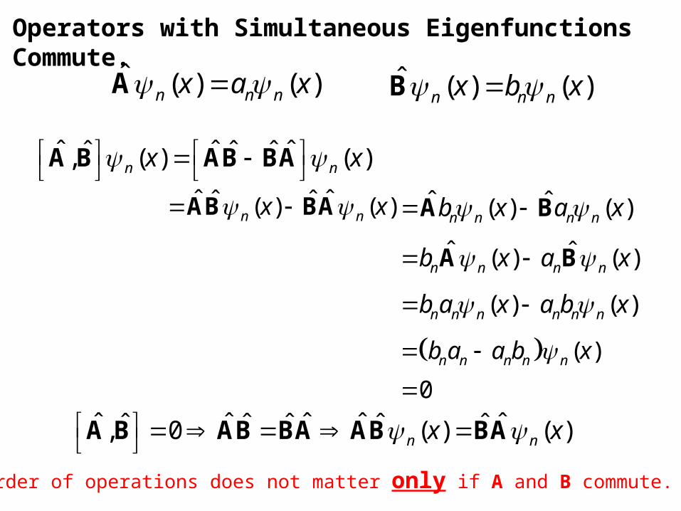
Operators with Simultaneous Eigenfunctions Commute.

ˆ ( ) ( )n n nx a x A ˆ ( ) ( )n n nx b x B

ˆ ˆ ˆˆ ˆ ˆ, ( ) ( )n nx x A B AB BA

ˆ ˆˆ ˆ( ) ( )n nx x AB BA ˆ ˆ( ) ( )n n n nb x a x A B

ˆ ˆ( ) ( )n n n nb x a x A B

( ) ( )n n n n n nb a x a b x

( )

0n n n n nb a a b x

ˆ ˆ ˆ ˆ ˆˆ ˆ ˆ ˆ ˆ, 0 ( ) ( )n nx x A B AB BA AB BA

Order of operations does not matter only if A and B commute.

* *ˆ ˆ( ) ( ) ( ) ( ) ( )n

S

t x t x t dx H H

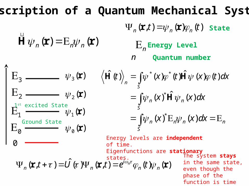
Description of a Quantum Mechanical System

( ) ( )n n n H r r

n

( , ) ( ) ( )n n nt t r r

Energy Level

State

* ˆ( ) ( )n n

S

x x dx H

Energy levels are independent of time.Eigenfunctions are stationary states.

*( ) ( )n n n n

S

x x dx 01

3

2

0 ( ) r

1( ) r

2 ( ) r

3( ) r

The system stays in the same state, even though the phase of the function is time dependent.

Ground State

1st excited State

0

n Quantum number

ˆ( , ) ( ) ( , ) ( ) ( )nin n n nt U t e t r r r

Expectation Values Revisited

* ˆˆ ˆ( ) ( ,0) ( ) ( ,0)n n

R

t x t x dx U O U

* ˆ( ) ( , ) ( , )n n

R

t x t x t dx O O

*ˆ ˆ

ˆ( ,0) ( ,0) xi t i t

n n

R

e x e x d

H H

O

ˆ ˆ

* ˆ( ,0) ( ,0)i t i t

n n

R

x e e x dx

H H

O

ˆ ˆ

* ˆ( ,0) ( ,0) xi t i t

n n

R

x e e x d

H H

O

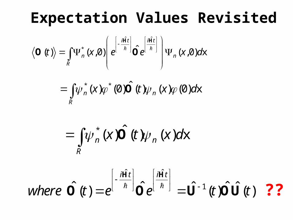
Expectation Values Revisitedˆ ˆ

* ˆ( ) ( ,0) ( ,0) xi t i t

n n

R

t x e e x d

H H

O O

* * ˆ( ) (0) ( ) ( ) (0) xn n

R

x t x d O

* ˆ( ) ( ) ( ) xn n

R

x t x d O

ˆ ˆ

1ˆ ˆ ˆˆ ˆ( ) ( ) ( )i t i t

where t e e t t

H H

O O U OU ??

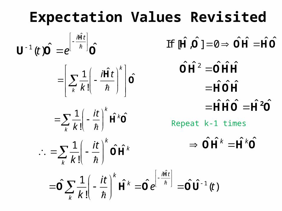
Expectation Values Revisited

1 ˆˆ!

kk

k

it

k

H O

ˆ ˆ ˆˆ ˆ ˆIf [ , ] 0 H O OH HO

ˆ1 ˆ!

k

k

i t

k

H

O

2ˆ ˆˆ ˆ ˆ

ˆˆ ˆ

ˆ ˆˆ ˆ ˆ

2

OH OHH

HOH

HHO H O

ˆ ˆˆ ˆk k OH H O

Repeat k-1 times

1 ˆ ˆ!

kk

k

it

k

OH

ˆ

1 ˆ ˆ( )i t

t e

H

U O O

ˆ

11ˆ ˆ ˆˆ ˆ ( )!

i tkk

k

ite t

k

H

O H O OU

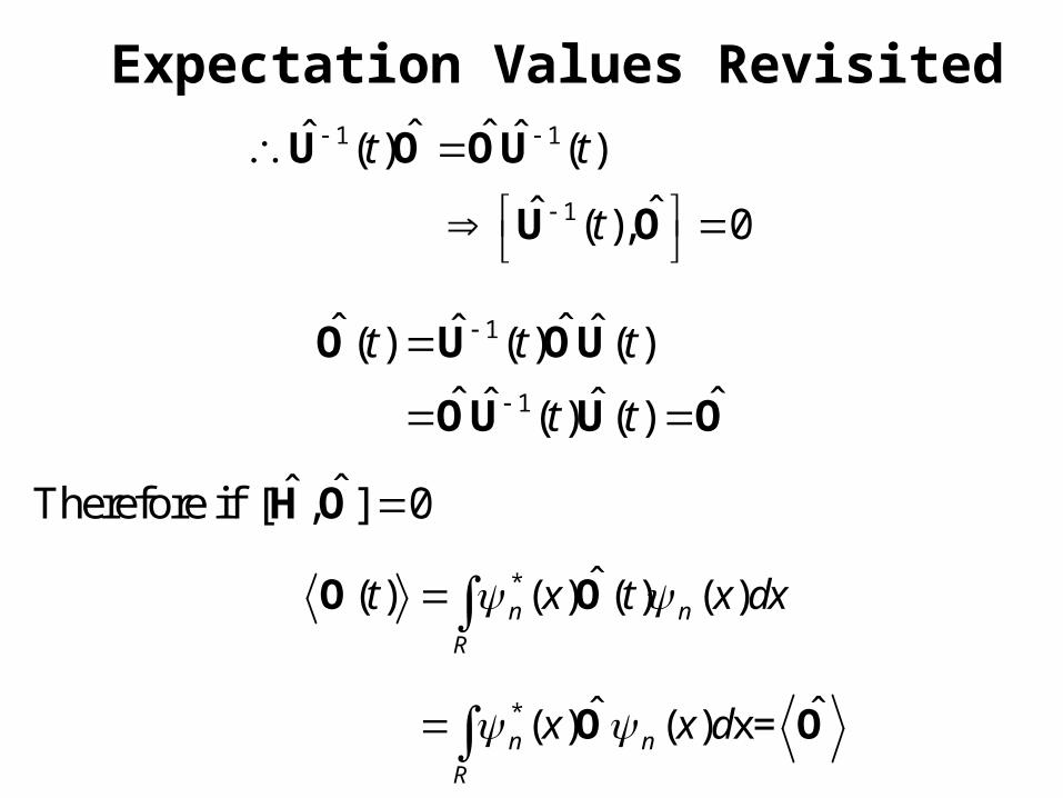
Expectation Values Revisited

1

1

ˆ ˆˆ ˆ( ) ( ) ( )

ˆ ˆˆ ˆ( ) ( )

t t t

t t

O U OU

OU U O

*

*

ˆ( ) ( ) ( ) ( )

ˆ ˆ( ) ( ) x=

n n

R

n n

R

t x t x dx

x x d

O O

O O

1 1

1

ˆ ˆˆ ˆ( ) ( )

ˆˆ ( ), 0

t t

t

U O OU

U O

ˆˆTherefore if [ , ] 0H O

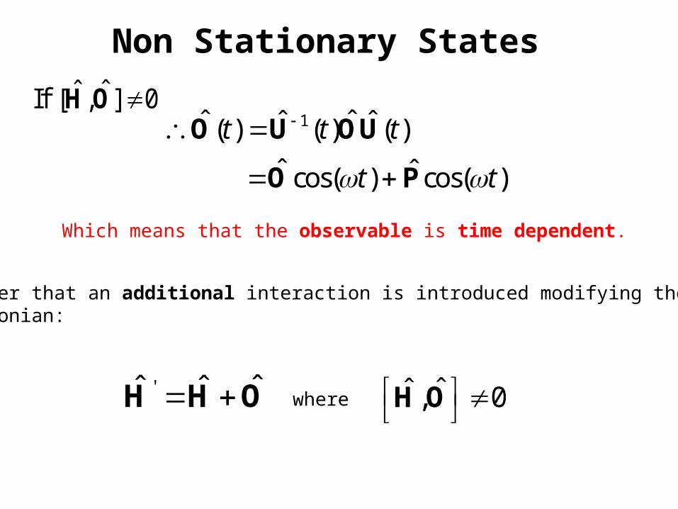
Non Stationary States

1ˆ ˆˆ ˆ( ) ( ) ( )t t t O U OUˆˆIf [ , ] 0H O

Which means that the observable is time dependent.

Consider that an additional interaction is introduced modifying the Hamiltonian:

' ˆˆ ˆ H H O ˆˆ , 0 H Owhere

ˆ ˆcos( ) cos( )t t O P

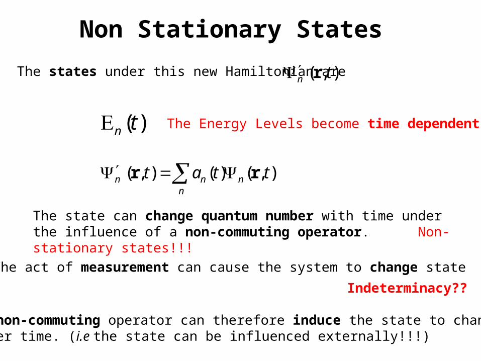
Non Stationary States

( , )n t r

( )n t The Energy Levels become time dependent

( , ) ( ) ( , )n n nn

t a t t r r

The state can change quantum number with time under the influence of a non-commuting operator. Non-stationary states!!!

A non-commuting operator can therefore induce the state to change over time. (i.e the state can be influenced externally!!!)

Indeterminacy??

The states under this new Hamiltonian are

The act of measurement can cause the system to change state