Acta Astronautica 140 (2017) 255–263

Contents lists available at ScienceDirect

Acta Astronautica

journal homepage: www.elsevier .com/locate/actaastro

A Cartesian relative motion approach to optimal formation flight usingLorentz forces and impulsive thrusting

Behrad Vatankhahghadim, Christopher J. Damaren *

University of Toronto Institute for Aerospace Studies, 4925 Dufferin Street, Toronto, Ontario, M3H 5T6, Canada

A R T I C L E I N F O

Keywords:Spacecraft formation flightLorentz-augmented formationOptimal hybrid controlRelative Cartesian dynamics

* Corresponding author.E-mail addresses: behrad.vatankhahghadim@mail.utor

http://dx.doi.org/10.1016/j.actaastro.2017.08.023Received 1 June 2017; Received in revised form 20 JulyAvailable online 30 August 20170094-5765/© 2017 IAA. Published by Elsevier Ltd. All ri

A B S T R A C T

Hybrid combination of Lorentz forces and impulsive thrusts, provided by modulating spacecraft's electrostaticcharge and propellant usage, respectively, is proposed for formation flight applications. A hybrid linear quadraticregulator, previously proposed in another work using a differential orbital elements-based model, is reconsideredfor a Cartesian coordinates-based description of the spacecraft's relative states. In addition, the effects of adoptingcircular versus elliptic reference solutions on the performance of the controller are studied. Numerical simulationresults are provided to demonstrate the functionality of the proposed controller in the presence of J2 perturba-tions, and to illustrate the improvements gained by assuming an elliptic reference and incorporating auxiliaryimpulsive thrusts.

1. Introduction

Formation flight of spacecraft, involving groups of multiple satellitesthat orbit in proximity of each other, has seen a lot of renewed interest inrecent years. This is particularly because of the improvements they offerover single-spacecraft missions in terms of affordability and robustness,and is facilitated by recent technological and scientific developments thatenable reliable formationmissions. One potential approach for spacecraftto achieve and maintain formation is via Lorentz-augmented control. Theidea of using Lorentz forces generated by the interaction of actively-modulated charges on a spacecraft with the geomagnetic field in orderto produce useful thrust was first proposed in Ref. [1].

In Ref. [2], analytical solutions of the equations of motion forLorentz-augmented spacecraft in various situations were provided;however, only constant specific charges and circular reference frameswere considered. The equations of motion linearized relative to a circularreference orbit were presented in Refs. [3,4], and are known as theHill-Clohessy-Wiltshire (HCW) equations. Also using a spherical co-ordinates description similarly to [2], a three-spacecraft formationreconfiguration problem was considered in Ref. [5], but assuming pro-portional derivative-type feedback control provided by modulating thespecific charge. Abandoning the circularity assumption on the chiefspacecraft's orbit, Ref. [6] considered both circular and elliptic referencesusing Cartesian coordinates for relative motion. In that work, step-wisecharge control based on the linearized model, as well sequential

onto.ca (B. Vatankhahghadim), dama

2017; Accepted 21 August 2017

ghts reserved.

quadratic programming using the nonlinear model were proposed. Therelative motion equations that allow for elliptic reference orbits areknown as Tschauner-Hempel (TH) equations, and were provided in Refs.[7,8], among others.

In contrast to the use of spherical or Cartesian coordinates to describethe relative motion of spacecraft in formation, an alternative is to focuson the changes in the mean orbital elements, hence ignoring the short-term oscillations. Examples of past literature that make use of (mean)orbital elements (or their differences) for formation control are [9,10],and those of works that involve Lorentz-augmentation in particular are[11,12]. This approach is primarily motivated by the fact that, in manyformation flight missions, only secular changes are of importance whendetermining tracking errors. While recognizing the value of this approach(especially in the presence of J2 perturbations), the present authors havechosen to work directly with the Cartesian description of the spacecraft'sabsolute and relative positions. It is expected that such an approach willbe better suited to applications for which short-term errors do matter. Inorder to demonstrate the effectiveness of the proposed controller and itscomparability with the mean orbital elements-based techniques, J2 in-fluences are modelled in all simulation results to be presented. It is shownthat the required specific charge and thrust magnitudes are stillreasonable.

Hybrid formation control of spacecraft using continuous and impul-sive forces in tandem is considered in this paper, based on a Cartesiancoordinates-based model, and the methodology is applicable to both

ren@utias.utoronto.ca (C.J. Damaren).

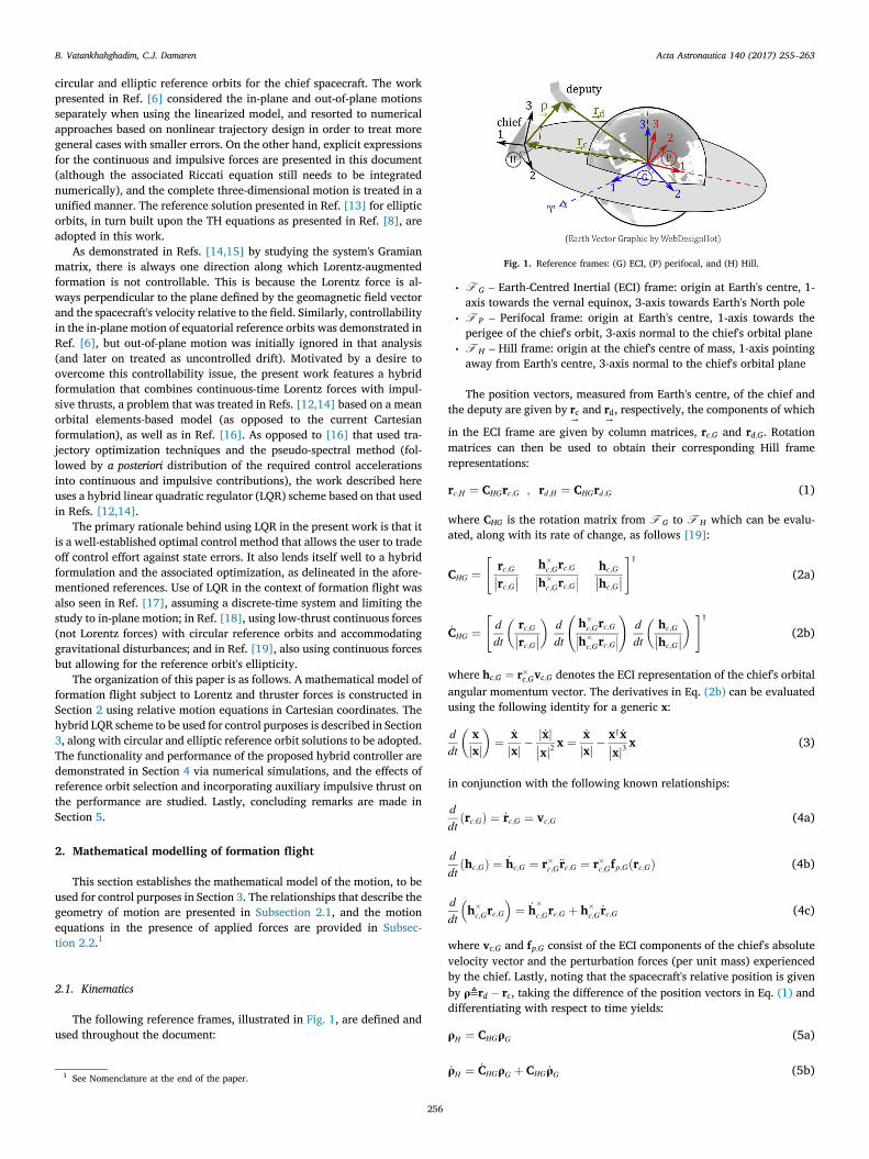
Fig. 1. Reference frames: (G) ECI, (P) perifocal, and (H) Hill.

B. Vatankhahghadim, C.J. Damaren Acta Astronautica 140 (2017) 255–263

circular and elliptic reference orbits for the chief spacecraft. The workpresented in Ref. [6] considered the in-plane and out-of-plane motionsseparately when using the linearized model, and resorted to numericalapproaches based on nonlinear trajectory design in order to treat moregeneral cases with smaller errors. On the other hand, explicit expressionsfor the continuous and impulsive forces are presented in this document(although the associated Riccati equation still needs to be integratednumerically), and the complete three-dimensional motion is treated in aunified manner. The reference solution presented in Ref. [13] for ellipticorbits, in turn built upon the TH equations as presented in Ref. [8], areadopted in this work.

As demonstrated in Refs. [14,15] by studying the system's Gramianmatrix, there is always one direction along which Lorentz-augmentedformation is not controllable. This is because the Lorentz force is al-ways perpendicular to the plane defined by the geomagnetic field vectorand the spacecraft's velocity relative to the field. Similarly, controllabilityin the in-plane motion of equatorial reference orbits was demonstrated inRef. [6], but out-of-plane motion was initially ignored in that analysis(and later on treated as uncontrolled drift). Motivated by a desire toovercome this controllability issue, the present work features a hybridformulation that combines continuous-time Lorentz forces with impul-sive thrusts, a problem that was treated in Refs. [12,14] based on a meanorbital elements-based model (as opposed to the current Cartesianformulation), as well as in Ref. [16]. As opposed to [16] that used tra-jectory optimization techniques and the pseudo-spectral method (fol-lowed by a posteriori distribution of the required control accelerationsinto continuous and impulsive contributions), the work described hereuses a hybrid linear quadratic regulator (LQR) scheme based on that usedin Refs. [12,14].

The primary rationale behind using LQR in the present work is that itis a well-established optimal control method that allows the user to tradeoff control effort against state errors. It also lends itself well to a hybridformulation and the associated optimization, as delineated in the afore-mentioned references. Use of LQR in the context of formation flight wasalso seen in Ref. [17], assuming a discrete-time system and limiting thestudy to in-plane motion; in Ref. [18], using low-thrust continuous forces(not Lorentz forces) with circular reference orbits and accommodatinggravitational disturbances; and in Ref. [19], also using continuous forcesbut allowing for the reference orbit's ellipticity.

The organization of this paper is as follows. A mathematical model offormation flight subject to Lorentz and thruster forces is constructed inSection 2 using relative motion equations in Cartesian coordinates. Thehybrid LQR scheme to be used for control purposes is described in Section3, along with circular and elliptic reference orbit solutions to be adopted.The functionality and performance of the proposed hybrid controller aredemonstrated in Section 4 via numerical simulations, and the effects ofreference orbit selection and incorporating auxiliary impulsive thrust onthe performance are studied. Lastly, concluding remarks are made inSection 5.

2. Mathematical modelling of formation flight

This section establishes the mathematical model of the motion, to beused for control purposes in Section 3. The relationships that describe thegeometry of motion are presented in Subsection 2.1, and the motionequations in the presence of applied forces are provided in Subsec-tion 2.2.1

2.1. Kinematics

The following reference frames, illustrated in Fig. 1, are defined andused throughout the document:

1 See Nomenclature at the end of the paper.

256

∙ F G – Earth-Centred Inertial (ECI) frame: origin at Earth's centre, 1-axis towards the vernal equinox, 3-axis towards Earth's North pole

∙ F P – Perifocal frame: origin at Earth's centre, 1-axis towards theperigee of the chief's orbit, 3-axis normal to the chief's orbital plane

∙ F H – Hill frame: origin at the chief's centre of mass, 1-axis pointingaway from Earth's centre, 3-axis normal to the chief's orbital plane

The position vectors, measured from Earth's centre, of the chief andthe deputy are given by rc

→and rd

→, respectively, the components of which

in the ECI frame are given by column matrices, rc;G and rd;G. Rotationmatrices can then be used to obtain their corresponding Hill framerepresentations:

rc;H ¼ CHGrc;G ; rd;H ¼ CHGrd;G (1)

where CHG is the rotation matrix from F G to F H which can be evalu-ated, along with its rate of change, as follows [19]:

CHG ¼"

rc;G��rc;G�� h�c;Grc;G���h�c;Grc;G

���hc;G��hc;G

��#⊺

(2a)

_CHG ¼"ddt

�rc;G��rc;G��

�ddt

h�c;Grc;G���h�c;Grc;G

���!

ddt

�hc;G��hc;G

��� #⊺

(2b)

where hc;G ¼ r�c;Gvc;G denotes the ECI representation of the chief's orbitalangular momentum vector. The derivatives in Eq. (2b) can be evaluatedusing the following identity for a generic x:

ddt

�xjxj�

¼ _xjxj �

j _xj��xj2 x ¼ _xjxj �

x⊺ _x��xj3 x (3)

in conjunction with the following known relationships:

ddtðrc;GÞ ¼ _rc;G ¼ vc;G (4a)

ddtðhc;GÞ ¼ _hc;G ¼ r�c;G€rc;G ¼ r�c;Gfp;Gðrc;GÞ (4b)

ddt

�h�c;Grc;G

�¼ _h

�c;Grc;G þ h�

c;G _rc;G (4c)

where vc;G and fp;G consist of the ECI components of the chief's absolutevelocity vector and the perturbation forces (per unit mass) experiencedby the chief. Lastly, noting that the spacecraft's relative position is givenby ρ≜rd � rc, taking the difference of the position vectors in Eq. (1) anddifferentiating with respect to time yields:

ρH ¼ CHGρG (5a)

_ρH ¼ _CHGρG þ CHG _ρG (5b)

B. Vatankhahghadim, C.J. Damaren Acta Astronautica 140 (2017) 255–263

which will be used in simulation to obtain the relative states at each time.

2.2. Dynamics

The equations of motion that describe the system of interest's dy-namics are given by Newton's law of gravitation:

€rc;G ¼ �μer3c

rc;G þ fp;Gðrc;GÞ (6a)

€rd;G ¼ �μer3d

rd;G þ fp;Gðrd;GÞ þ f ct;G þ fds;G (6b)

where r≜jrGj ¼ jrH j and μe ¼ 3.986 � 1014 m3∕s2 is Earth's standardgravitational parameter, and spatial dependence of the perturbationforce per unit mass, fp, is taken into account by representing it as afunction of position. Assuming only the deputy is actuated, continuous-and discrete-time control forces per unit mass are denoted by fct;G andfds;G, respectively. Subtracting Eq. (6b) from Eq. (6a) and using rd;G ¼ρG þ rc;G by definition yields the following relative dynamics:

€ρG ¼�μeðρG þ rc;GÞ��ρG þ rc;Gj3þ μer3crc;G þ

�fp;GðρG þ rc;GÞ� fp;Gðrc;GÞ

�þ f ct;G þ fds;G

(7)

The primary perturbation source for spacecraft in formation is the J2perturbation resulting from the effects of Earth's non-spherical shape onits gravitational field [10,16]. An analytic expression for estimating theperturbation force, obtained by taking the gradient of the correspondingscalar field, is given by (as expressed in F G) [20]:

fp;G ¼ 3μeJ2R2e

2��rGj5

" 5ðr⊺Gbg3Þ2��rGj2 � 1

!rG � 2ðr⊺Gbg3Þbg3

#(8)

where J2 ¼ 1.083 � 10�3 for Earth represents the most dominantperturbation term associated with Earth's oblate shape, andRe ¼ 6.378 � 106 m is Earth's radius. The unit column matrix,bg3 ¼ ½0 0 1�⊺, denotes the basis vector along the 3-axis of the ECI frameshown in Fig. 1, directed towards the North pole.

Lastly, the continuous- and discrete-time control forces per unit mass,assumed to be provided by the Lorentz force on the deputy caused by anactively-controlled accumulated charge, qðtÞ, and impulsive thrusters,respectively, are given by (as expressed in F G):

f E v vbb ω r (9a)

fds;GðtÞ ¼X∞k¼1

νk;Gδðt � tkÞ (9b)

where bq≜q∕md is defined for specific charge per unit deputy mass, md,and vrel;G represents the spacecraft's velocity relative to Earth's magneticfield. The electrical field strength, EG, is assumed to be negligible. Inaddition, ωe;G ¼ 360:9856 bg3 deg∕s and bG are the inertial componentsof Earth's angular velocity (about its own axis of rotation) and magneticfield vector (obtained upon assuming a tilted dipole model as describedin Appendix H of [21]). The Dirac delta function, δ(t), centred at each

257

impulse time, tkwith k 2 N, is used in conjunction with gain values, νk, torepresent three-dimensional impulsive thrust forces per unit mass.

3. Formation control

In preparation for application of the hybrid LQR scheme of [14] to theCartesian formation flight problem in hand, the motion model of Section2 is first linearized in Subsection 3.1. Two different, yet related, referenceorbit solutions that assume circular or elliptic chief orbits (based on theHCW and TH equations, respectively) are selected in Subsection 3.2, andtreating deviations from these solutions as relative state errors, Subsec-tion 3.3 completes the description of the control scheme by determiningthe appropriate continuous and impulsive control inputs. It should benoted that both of these solutions are linearized and are expected to workwell for small enough formations [13], but higher order solutions may bedesired for large relative distances or highly elliptic reference orbits.

3.1. Linearized control system

The relative dynamics in Eq. (7) can be expressed in state-space formas a system of continuous- and discrete-time equations. To this end,assuming a circular orbit for the chief and linearizing Eq. (7) about thiscircular reference yields the following model as expressed in F H , basedon the HCW equations in Refs. [3,4]:

_ρHðtÞ€ρHðtÞ

_xðtÞ

≈ 03�3 13�3

M N

|fflfflfflfflfflfflfflfflfflffl{zfflfflfflfflfflfflfflfflfflffl}Act

_ρHðtÞ€ρHðtÞ

xðtÞ

þ"

03�1

�CHGðtÞb�GðtÞ

�vc;GðtÞ �ω�

E;Grc;GðtÞ� #

|fflfflfflfflfflfflfflfflfflfflfflfflfflfflfflfflfflfflfflfflfflfflfflfflfflfflfflfflfflfflfflfflfflfflfflffl{zfflfflfflfflfflfflfflfflfflfflfflfflfflfflfflfflfflfflfflfflfflfflfflfflfflfflfflfflfflfflfflfflfflfflfflffl}Bct ðtÞ

½ bq �uct ðtÞ

; t≠tk

(10a)

ρH

�tþk

_ρH

�tþk

xðtþk Þ≈ 13�3 03�3

03�3 13�3

|fflfflfflfflfflfflfflfflfflffl{zfflfflfflfflfflfflfflfflfflffl}

Ads

ρH

�t�k

_ρH

�t�k

xðt�k Þþ03�3

13�3

|fflfflfflffl{zfflfflfflffl}

Bds

½ νk �uds;k

; t ¼ tk

(10b)

where the deputy-related quantities in Eq. (9a) are replaced by chief-

related ones, consistent with the linearity assumption of rc;H≈rd;H . Inorder to assess up to what relative distance is the assumption valid thatbG is the same at both chief and deputy locations, a numerical study wasperformed: the orbit-averaged value of max1�i�3f

��ΔbG;i∕bc;G;i��g was

determined for the ith component of bc;G and its variation,ΔbG;i≜bd;G;i � bc;G;i, over a circular region (in the hill frame's yz-plane)centred at the chief's location. Using the reference orbits considered inSection 4, the value of this metric does not exceed 1% for relative dis-tances of less than 6 km.

The constant matrices M and N are given by:

B. Vatankhahghadim, C.J. Damaren Acta Astronautica 140 (2017) 255–263

M ¼24 3n2 0 0

0 0 00 0 �n2

35 ; N ¼24 0 2n 0�2n 0 00 0 0

35 (11)

where n≜�μe∕r3c

1∕2 is the mean orbital motion of the chief.

3.2. Reference orbit

A special family of periodic solutions to Eq. (10a) for the uncontrolledcase of uct≡0, known as the Projected Circular Orbit (PCO) solution, isgiven by Ref. [22]:

ρref ;H ¼

26664Rpco

2sinðnt þ α0Þ

Rpco cosðnt þ α0ÞRpco sinðnt þ α0Þ

37775 (12)

where Rpco is the radius of the target PCO, and α0 is the initial phase anglein the resulting circle. The corresponding relative velocity is obtained bydifferentiating Eq. (12) with respect to time:

_ρref ;H ¼

26664Rpco

2n cosðnt þ α0Þ

�Rpcon sinðnt þ α0ÞRpcon cosðnt þ α0Þ

37775 (13)

Provided in Ref. [13] is an extension of the above results to ellipticreference orbits, where the homogeneous solution to a lineartime-varying set of equations analogous to the HCW equations in Eq.(10a) is provided. Selecting the integration constants in that expressionin a certain way collapses it down to the following form [19]:

ρref ;H ¼

2666666664

Rpco

2cosðθÞ

�Rpco

2sinðθÞ

�2þ e cosðθÞ1þ e cosðθÞ

�Rpco

�cosðθÞ

1þ e cosðθÞ�

3777777775(14)

where θ is the chief's true anomaly in its orbit, as measured in the peri-focal reference frame, F P; and e is the chief orbit's eccentricity. Thereader should note that setting e ¼ 0 in Eq. (14) results in recovering the

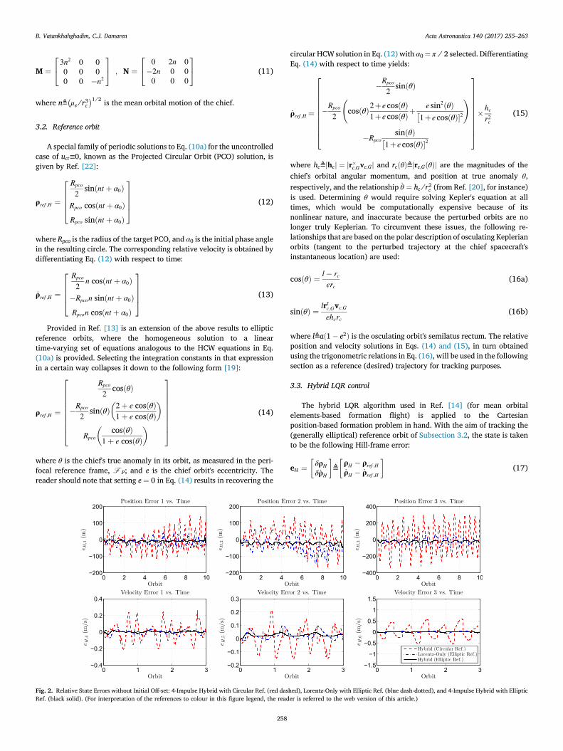
Fig. 2. Relative State Errors without Initial Off-set: 4-Impulse Hybrid with Circular Ref. (red dasRef. (black solid). (For interpretation of the references to colour in this figure legend, the read

258

circular HCW solution in Eq. (12) with α0¼ π ∕ 2 selected. DifferentiatingEq. (14) with respect to time yields:

_ρref ;H ¼

26666666664

�Rpco

2sinðθÞ

�Rpco

2

cosðθÞ2þe cosðθÞ

1þe cosðθÞþe sin2ðθÞ�

1þ e cosðθÞ�2!

�RpcosinðθÞ�

1þe cosðθÞ�2

37777777775�hcr2c

(15)

where hc≜jhcj ¼ jr�c;Gvc;Gj and rcðθÞ≜jrc;GðθÞj are the magnitudes of thechief's orbital angular momentum, and position at true anomaly θ,respectively, and the relationship _θ ¼ hc∕r2c (from Ref. [20], for instance)is used. Determining θ would require solving Kepler's equation at alltimes, which would be computationally expensive because of itsnonlinear nature, and inaccurate because the perturbed orbits are nolonger truly Keplerian. To circumvent these issues, the following re-lationships that are based on the polar description of osculating Keplerianorbits (tangent to the perturbed trajectory at the chief spacecraft'sinstantaneous location) are used:

cosðθÞ ¼ l� rcerc

(16a)

sinðθÞ ¼ lr⊺c;Gvc;G

ehcrc(16b)

where l≜að1� e2Þ is the osculating orbit's semilatus rectum. The relativeposition and velocity solutions in Eqs. (14) and (15), in turn obtainedusing the trigonometric relations in Eq. (16), will be used in the followingsection as a reference (desired) trajectory for tracking purposes.

3.3. Hybrid LQR control

The hybrid LQR algorithm used in Ref. [14] (for mean orbitalelements-based formation flight) is applied to the Cartesianposition-based formation problem in hand. With the aim of tracking the(generally elliptical) reference orbit of Subsection 3.2, the state is takento be the following Hill-frame error:

eH ¼δρH

δ _ρH

≜ρH � ρref ;H_ρH � _ρref ;H

(17)

hed), Lorentz-Only with Elliptic Ref. (blue dash-dotted), and 4-Impulse Hybrid with Ellipticer is referred to the web version of this article.)

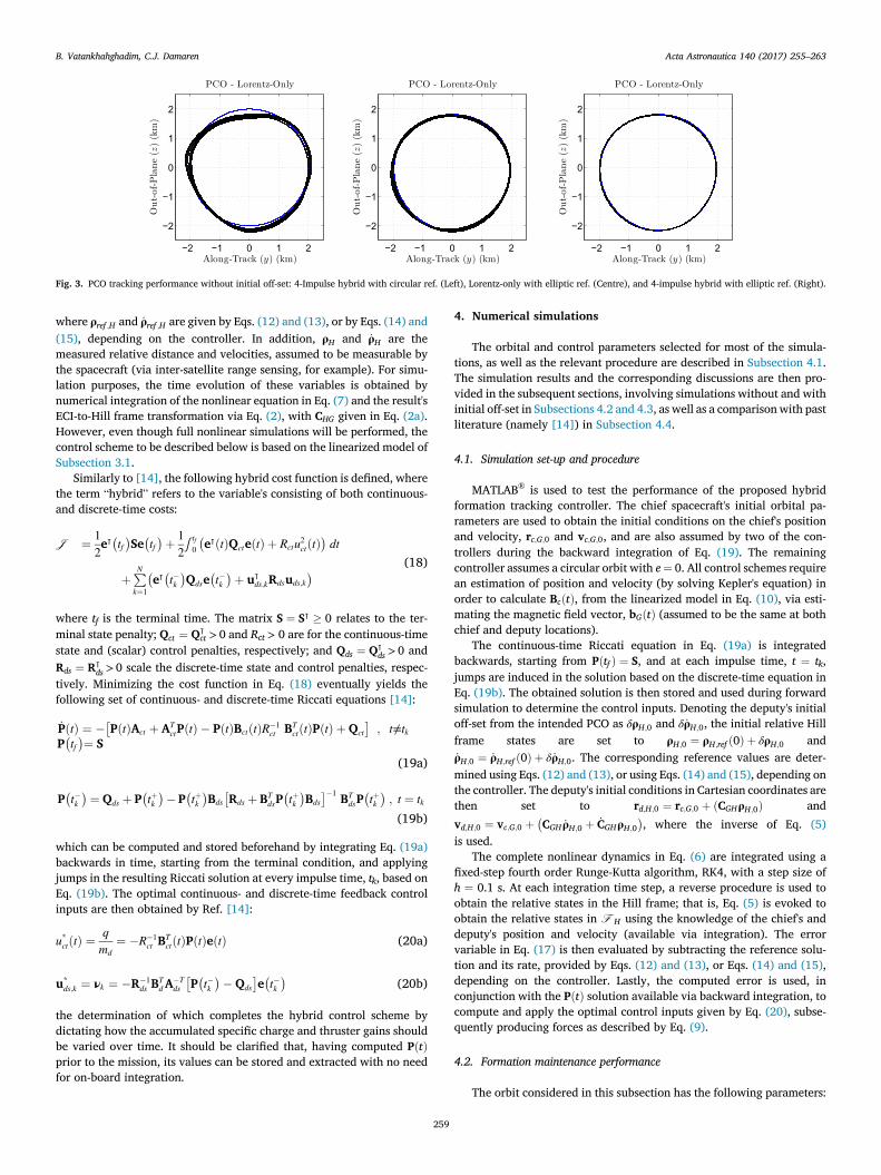
Fig. 3. PCO tracking performance without initial off-set: 4-Impulse hybrid with circular ref. (Left), Lorentz-only with elliptic ref. (Centre), and 4-impulse hybrid with elliptic ref. (Right).

B. Vatankhahghadim, C.J. Damaren Acta Astronautica 140 (2017) 255–263

where ρref ;H and _ρref ;H are given by Eqs. (12) and (13), or by Eqs. (14) and(15), depending on the controller. In addition, ρH and _ρH are themeasured relative distance and velocities, assumed to be measurable bythe spacecraft (via inter-satellite range sensing, for example). For simu-lation purposes, the time evolution of these variables is obtained bynumerical integration of the nonlinear equation in Eq. (7) and the result'sECI-to-Hill frame transformation via Eq. (2), with CHG given in Eq. (2a).However, even though full nonlinear simulations will be performed, thecontrol scheme to be described below is based on the linearized model ofSubsection 3.1.

Similarly to [14], the following hybrid cost function is defined, wherethe term “hybrid” refers to the variable's consisting of both continuous-and discrete-time costs:

J ¼ 12e⊺�tf Se�tf þ 1

2∫ tf0

�e⊺ðtÞQcteðtÞ þ Rctu2ctðtÞ

dt

þPNk¼1

�e⊺�t�k Qdse

�t�k þ u⊺

ds;kRdsuds;k

(18)

where tf is the terminal time. The matrix S ¼ S⊺ � 0 relates to the ter-minal state penalty; Qct ¼ Q⊺

ct > 0 and Rct > 0 are for the continuous-timestate and (scalar) control penalties, respectively; and Qds ¼ Q⊺

ds >0 andRds ¼ R⊺

ds >0 scale the discrete-time state and control penalties, respec-tively. Minimizing the cost function in Eq. (18) eventually yields thefollowing set of continuous- and discrete-time Riccati equations [14]:

_PðtÞ ¼ ��PðtÞAct þ ATctPðtÞ � PðtÞBctðtÞR�1

ct BTctðtÞPðtÞ þQct

�; t≠tk

P�tf ¼ S

(19a)

P�t�k ¼ Qds þ P

�tþk � P

�tþk Bds

�Rds þBT

dsP�tþk Bds

��1 BTdsP�tþk ; t ¼ tk(19b)

which can be computed and stored beforehand by integrating Eq. (19a)backwards in time, starting from the terminal condition, and applyingjumps in the resulting Riccati solution at every impulse time, tk, based onEq. (19b). The optimal continuous- and discrete-time feedback controlinputs are then obtained by Ref. [14]:

u*ctðtÞ ¼qmd

¼ �R�1ct B

TctðtÞPðtÞeðtÞ (20a)

u*ds;k ¼ νk ¼ �R�1

ds BTdA

�Tds

�P�t�k �Qds

�e�t�k

(20b)

the determination of which completes the hybrid control scheme bydictating how the accumulated specific charge and thruster gains shouldbe varied over time. It should be clarified that, having computed PðtÞprior to the mission, its values can be stored and extracted with no needfor on-board integration.

259

4. Numerical simulations

The orbital and control parameters selected for most of the simula-tions, as well as the relevant procedure are described in Subsection 4.1.The simulation results and the corresponding discussions are then pro-vided in the subsequent sections, involving simulations without and withinitial off-set in Subsections 4.2 and 4.3, as well as a comparisonwith pastliterature (namely [14]) in Subsection 4.4.

4.1. Simulation set-up and procedure

MATLAB® is used to test the performance of the proposed hybridformation tracking controller. The chief spacecraft's initial orbital pa-rameters are used to obtain the initial conditions on the chief's positionand velocity, rc;G;0 and vc;G;0, and are also assumed by two of the con-trollers during the backward integration of Eq. (19). The remainingcontroller assumes a circular orbit with e¼ 0. All control schemes requirean estimation of position and velocity (by solving Kepler's equation) inorder to calculate BcðtÞ, from the linearized model in Eq. (10), via esti-mating the magnetic field vector, bGðtÞ (assumed to be the same at bothchief and deputy locations).

The continuous-time Riccati equation in Eq. (19a) is integratedbackwards, starting from Pðtf Þ ¼ S, and at each impulse time, t ¼ tk,jumps are induced in the solution based on the discrete-time equation inEq. (19b). The obtained solution is then stored and used during forwardsimulation to determine the control inputs. Denoting the deputy's initialoff-set from the intended PCO as δρH;0 and δ _ρH;0, the initial relative Hillframe states are set to ρH;0 ¼ ρH;ref ð0Þ þ δρH;0 and_ρH;0 ¼ _ρH;ref ð0Þ þ δ _ρH;0. The corresponding reference values are deter-mined using Eqs. (12) and (13), or using Eqs. (14) and (15), depending onthe controller. The deputy's initial conditions in Cartesian coordinates arethen set to rd;H;0 ¼ rc;G;0 þ ðCGHρH;0Þ and

vd;H;0 ¼ vc;G;0 þ�CGH _ρH;0 þ _CGHρH;0

, where the inverse of Eq. (5)

is used.The complete nonlinear dynamics in Eq. (6) are integrated using a

fixed-step fourth order Runge-Kutta algorithm, RK4, with a step size ofh ¼ 0.1 s. At each integration time step, a reverse procedure is used toobtain the relative states in the Hill frame; that is, Eq. (5) is evoked toobtain the relative states in F H using the knowledge of the chief's anddeputy's position and velocity (available via integration). The errorvariable in Eq. (17) is then evaluated by subtracting the reference solu-tion and its rate, provided by Eqs. (12) and (13), or Eqs. (14) and (15),depending on the controller. Lastly, the computed error is used, inconjunction with the PðtÞ solution available via backward integration, tocompute and apply the optimal control inputs given by Eq. (20), subse-quently producing forces as described by Eq. (9).

4.2. Formation maintenance performance

The orbit considered in this subsection has the following parameters:

Fig. 4. Estimation of Electrostatic Charge and Thrust Δv Required without Initial Off-Set: Lorentz-Only with Elliptic Ref. (blue dash-dotted) and 4-Impulse Hybrid with Elliptic Ref. (blacksolid). (For interpretation of the references to colour in this figure legend, the reader is referred to the web version of this article.)

B. Vatankhahghadim, C.J. Damaren Acta Astronautica 140 (2017) 255–263

fa; e; i;ω;Ω; t0g ¼ f7092 km; 0:1; 0 rad; π∕4 rad; π∕4 rad; 0 sgThe terminal penalty for the LQR is set to Pðtf Þ ¼ S ¼ 106 � 16�6. The

continuous-time penalty variables, used for all controllers considered inthis subsection, are set to Qct ¼ blockdiagf102 � 13�3; 105 � 13�3g andRct ¼ 1010; while the discrete-time penalties, pertinent to the hybridcontroller that incorporate impulsive thrusts, are tuned to be Qds ¼blockdiagf102 � 13�3;105 � 13�3g and Rds ¼ 1010 � 13�3.

Shown in Fig. 2 are the relative position and velocity tracking errors

(in F H) over 10 orbits, starting with no initial off-set (δρH;0 ¼ δρ̇ H;0 ¼ 0)and using three controllers: a four-impulse hybrid controller (red dashed)that assumes a circular reference orbit, a Lorentz-only controller with noimpulses (blue dash-dotted) that assumes an elliptic reference orbit, anda four-impulse hybrid controller (black solid) that also assumes an ellipticreference. For the hybrid cases, the impulses are applied in intervals ofT∕4 starting from t ¼ 0. Fig. 3 shows the resulting tracking performanceas viewed along the x-direction, in the plane in which a PCO of radiusRpco ¼ 2 km is desired. As evident from both figures, for the elliptic orbitconsidered and using the current set of penalties, the formation controlperformance is significantly enhanced by using the elliptic correction tothe HCW equations, and further improvements ensue by incorporatingimpulses via the proposed hybrid algorithm.

Fig. 4 shows how much resources (electrostatic charge and thrust Δv)are expected to be required for the Lorentz-only and hybrid cases that useelliptic references, both of which are feasible with current technologies,considering a generally-acceptable range of 10�2 � 10�3 C ∕ kg forspecific charge [1,5]. As evident from this figure, reductions in specificcharge ensue from incorporating impulses, of course at the cost of fuelconsumption. The reader should not be alarmed by the increasing valuesof the resources required while approaching 10 orbits, as this does notsuggest instability: the periodicity of the system (considering its magneticfield variations using the current orbital elements) is 14 orbits, and asimilar beat-like pattern repeats with this period. Bounded motions wereverified for even as long as 20 orbits. Part of this sudden increase is also

Table 1Performance, without initial off-set, of 4-impulse hybrid with circular ref., Lorentz-onlywith elliptic ref., and 4-impulse hybrid with elliptic ref. Controllers over 10T.

Param. Description 4-Imp. Circ. Lorentz 4-Imp. Ellip. Unit

J 10T hybrid cost 1.92 � 1011 1.91 � 1010 4.50 � 109 –bq10T specificcharge

3.91 � 10�3 8.67 � 10�4 4.61 � 10�4 C/kg

k fctk10T Lorentz 6.06 � 10�4 1.73 � 10�4 1.01 � 10�4 N/kgk fdsk10T impulse 4.78 � 10�1 0 2.47 � 10�2 N⋅s∕kgk δρHk10T position

error1.81 � 102 7.56 � 101 3.21 � 101 m

k δρ̇ Hk10T velocityerror

3.87 � 10�1 8.45 � 10�2 3.60 � 10�2 m/s

260

due to the Riccati solution deviating from its steady-state pattern andapproaching the user-specified terminal value, S.

Presented in Table 1 are some performance measures that, in additionto the total cost, J (defined in Eq. (18)), also include some root mean

squared (RMS) norms defined generically as k

xk10T≜ffiffiffiffiffiffiffiffiffiffiffiffiffiffiffiffiffiffiffiffiffiffiffiffiffiffiffiffiffiffiffiffiffiffiffiffiffiffiffiffiffiffiffi�∫ 10T0 x⊺x dt

�∕ð10TÞ

rfor continuous variables, such that x is set

to fct , δρH , and δ _ρH for specific continuous force, relative position error,

and relative velocity error, respectively. Similarly, k

bqk10T≜ ffiffiffiffiffiffiffiffiffiffiffiffiffiffiffiffiffiffiffiffiffiffiffiffiffiffiffiffiffiffiffiffiffiffiffiffiffiffiffiffiffiffiffiffiffiffiffi∫ 10T0

�bqðtÞ2 dt�∕ð10TÞ

rdenotes the RMS of the specific charge.

For the impulsive force measure, an analogous discrete-time parameter is

defined as k fdsk10T≜ffiffiffiffiffiffiffiffiffiffiffiffiffiffiffiffiffiffiffiffiffiffiffiffiffiffiffiffiffiffiffiffiðPN

k¼1v⊺kvkÞ∕N

q. Table 1 shows more than 75%

and 57% reduction in the hybrid cost and relative position/velocity er-rors, respectively, as a result of adding impulsive thrusts. In addition,about 47% reduction is observed in the specific charge RMS as aconsequence.

4.3. Transient behaviour with initial off-set

As mentioned in Section 1, the main motivation for using impulsivethrusts as an auxiliary mechanism to complement the Lorentz force-basedformation control is overcoming the controllability issue associated withthe latter. This is illustrated in Figs. 5 and 6 that show the relative stateerrors and resource consumption expected from using the same Lorentz-only and four-impulse hybrid controllers as described in Subsection 4.2(with the same penalties and orbital parameters), but now with a non-zero initial condition; i.e. an initial off-set of δρ0 ¼ ½0:2 0:2 0:2� km and

δρ̇ H;0 ¼ 0 away from the desired PCO. As expected, the Lorentz-onlycontroller suffers significantly owing to its lack of controllability in onedirection at all times, whereas the hybrid controller is capable of elimi-nating the initial error and achieving the intended PCO formation. Thereader should keep in mind that the thrust Δv could be reduced if needbe, by more heavily penalizing the impulsive control effort viaincreasing Rds.

4.4. Comparison with previous results

In order to validate the results presented thus far and assess theperformance of the proposed controller against those previously pre-sented in literature, comparison is made against the simulation results of[14] (the control scheme of which was used in the present project). Thefollowing parameters based on the mean orbital elements used inRef. [14] are selected to allow for a meaningful comparison:

Fig. 5. Relative State Errors with Non-Zero Off-set: Lorentz-Only with Elliptic Ref. (blue dash-dotted), and 4-Impulse Hybrid with Elliptic Ref. (black solid). (For interpretation of thereferences to colour in this figure legend, the reader is referred to the web version of this article.)

Fig. 6. Estimation of Electrostatic Charge and Thrust Δv Required with Non-Zero Initial Off-set: Lorentz-Only with Elliptic Ref. (blue dash-dotted) and 4-Impulse Hybrid with EllipticRef. (black solid). (For interpretation of the references to colour in this figure legend, the reader is referred to the web version of this article.)

B. Vatankhahghadim, C.J. Damaren Acta Astronautica 140 (2017) 255–263

fa; e; i;ω;Ω; t0g ¼ f7092 km; 0:05; π∕2 rad; 0 rad; π rad; 0 sgA PCO of Rpco ¼ 1 km with no initial deputy off-set is chosen as the

formation objective. The LQR parameters are set toPðtf Þ ¼ S ¼ blockdiagf106 � 13�3;1010 � 13�3g, Rct ¼ 1013, andRds ¼ 1011 � 13�3. The state penalties are selected as suggested byRef. [14], setting Qct ¼ 105ðΞnzΞ⊺

nzÞ and Qds ¼ 4� 1011ðΞzΞ⊺zÞ. The

matrices Ξnz and Ξz consist of the eigenvectors respectively correspond-ing to the non-zero eigenvalues and the smallest (close to zero) eigen-value (related to the uncontrollable direction) of the controllabilityGramian of the continuous-time portion of the system, namely Eq. (10a).

Simulation results obtained over 10 orbits (where steady-state isreached) using twenty impulses per orbit (every T∕20, starting from

Fig. 7. Relative Position Errors with Non-Zero Off-set

261

t ¼ T∕40) are partly presented in Fig. 7 and compared in Table 2 againstsome values from Ref. [14]. The parameters jeH,ijmax represent the largestmagnitude of the error in the ith component of relative position. Theaveraged parameter jΔvjavg/orb denotes the mean of jνkj times thenumber of impulses per orbit, and k bqk10T as defined in Table 1 is an RMSmeasure of the specific charge (assuming RMS of the results in Ref. [14]does not change much when going from 10 orbits to 100 as reported inthat paper). The errors and specific charge required are comparable withor better than those of [14] overall, despite using a Cartesiancoordinates-based approach here instead of mean orbital elements, butthe latter is clearly superior in terms of fuel consumption. In addition,Fig. 7 (compared to Fig. 2 that features errors in the order of 20–40 musing four impulses) demonstrates that arbitrarily small tracking errors

using 20-Impulse Hybrid LQR with Elliptic Ref.

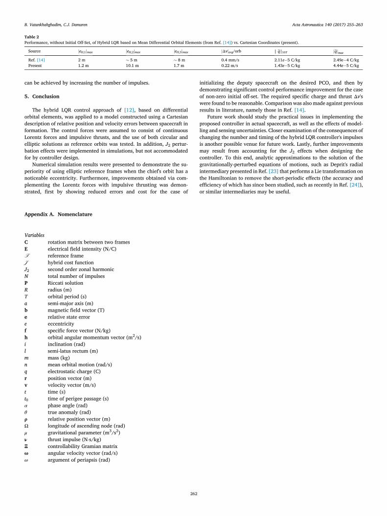
Table 2Performance, without Initial Off-Set, of Hybrid LQR based on Mean Differential Orbital Elements (from Ref. [14]) vs. Cartesian Coordinates (present).

Source jeH,1jmax jeH,2jmax jeH,3jmax jΔvjavg/orb k bqk10T jbqjmax

Ref. [14] 2 m � 5 m � 8 m 0.4 mm/s 2.11e�5 C/kg 2.49e�4 C/kgPresent 1.2 m 10.1 m 1.7 m 0.22 m/s 1.43e�5 C/kg 4.44e�5 C/kg

B. Vatankhahghadim, C.J. Damaren Acta Astronautica 140 (2017) 255–263

can be achieved by increasing the number of impulses.

5. Conclusion

The hybrid LQR control approach of [12], based on differentialorbital elements, was applied to a model constructed using a Cartesiandescription of relative position and velocity errors between spacecraft information. The control forces were assumed to consist of continuousLorentz forces and impulsive thrusts, and the use of both circular andelliptic solutions as reference orbits was tested. In addition, J2 pertur-bation effects were implemented in simulations, but not accommodatedfor by controller design.

Numerical simulation results were presented to demonstrate the su-periority of using elliptic reference frames when the chief's orbit has anoticeable eccentricity. Furthermore, improvements obtained via com-plementing the Lorentz forces with impulsive thrusting was demon-strated, first by showing reduced errors and cost for the case of

262

initializing the deputy spacecraft on the desired PCO, and then bydemonstrating significant control performance improvement for the caseof non-zero initial off-set. The required specific charge and thrust Δv'swere found to be reasonable. Comparison was also made against previousresults in literature, namely those in Ref. [14].

Future work should study the practical issues in implementing theproposed controller in actual spacecraft, as well as the effects of model-ling and sensing uncertainties. Closer examination of the consequences ofchanging the number and timing of the hybrid LQR controller's impulsesis another possible venue for future work. Lastly, further improvementsmay result from accounting for the J2 effects when designing thecontroller. To this end, analytic approximations to the solution of thegravitationally-perturbed equations of motions, such as Deprit's radialintermediary presented in Ref. [23] that performs a Lie transformation onthe Hamiltonian to remove the short-periodic effects (the accuracy andefficiency of which has since been studied, such as recently in Ref. [24]),or similar intermediaries may be useful.

Appendix A. Nomenclature

VariablesC rotation matrix between two framesE electrical field intensity (N/C)F reference frameJ hybrid cost functionJ2 second order zonal harmonicN total number of impulsesP Riccati solutionR radius (m)T orbital period (s)a semi-major axis (m)b magnetic field vector (T)e relative state errore eccentricityf specific force vector (N/kg)h orbital angular momentum vector (m2/s)i inclination (rad)l semi-latus rectum (m)m mass (kg)n mean orbital motion (rad/s)q electrostatic charge (C)r position vector (m)v velocity vector (m/s)t time (s)t0 time of perigee passage (s)α phase angle (rad)θ true anomaly (rad)ρ relative position vector (m)Ω longitude of ascending node (rad)μ gravitational parameter (m3/s2)ν thrust impulse (N⋅s/kg)Ξ controllability Gramian matrixω angular velocity vector (rad/s)ω argument of periapsis (rad)

B. Vatankhahghadim, C.J. Damaren Acta Astronautica 140 (2017) 255–263

Matrices1n�n an n � n identity matrix0m�n an m � n zero matrixOperatorsΔð⋅Þ variation (change) in a variableδ(t) Dirac delta functioncð⋅Þ normalized quantity

ð⋅Þ̇

differentiation with respect to timej⋅j Euclidean norm of a vectork ⋅ k root mean squared norm of a quantityð⋅Þ� skew-symmetric matrix operator

SubscriptsG in Earth-centred inertial frameH in Hill frameP in perifocal framec chief-relatedd deputy-relatede earth-relatedct continuous-timeds discrete-timep perturbation0 initial valuef final valuez corresponding to zero eigenvaluenz corresponding to nonzero eigenvalueavg average value of a quantitymax maximum value of a quantitypco projected circular orbitref referencerel relativenT computed over n orbital periods

Superscriptsð⋅Þþ post-impulse quantityð⋅Þ� pre-impulse quantity

ð⋅Þ* optimal quantity

References

[1] M.A. Peck, Prospects and challenges for lorentz-augmented orbits, in: Proceedingsof the AIAA Guidance, Navigation, and Control Conference and Exhibit, SanFrancisco, CA, Aug. 2005, http://dx.doi.org/10.2514/6.2005-5995.

[2] G.E. Pollock, J.W. Gangestad, J.M. Longuski, Analytical solutions for the relativemotion of spacecraft subject to lorentz force perturbations, Acta Astronaut. 68 (1–2)(Jan.-Feb. 2011) 204–217, http://dx.doi.org/10.1016/j.actaastro.2010.07.007.

[3] G.W. Hill, Researches in the lunar theory, Am. J. Math. 1 (1) (1878) 5–26, http://dx.doi.org/10.2307/2369430.

[4] W.H. Clohessy, R.S. Wiltshire, Terminal guidance system for satellite rendezvous,J. Aerosp. Sci. 27 (9) (Sept. 1960) 653–658, http://dx.doi.org/10.2514/8.8704.

[5] M.A. Peck, B. Streetman, C.M. Saaj, V. Lappas, Spacecraft formation flying usinglorentz forces, J. Br. Interplanet. Soc. 60 (Jul. 2007) 263–267.

[6] S. Tsujii, M. Bando, H. Yamakawa, Spacecraft formation flying dynamics andcontrol using the geomagnetic lorentz force, J. Guid. Control, Dyn. 36 (1) (Jan.-Feb.2013) 136–148, http://dx.doi.org/10.2514/1.57060.

[7] J. Tschauner, Elliptic orbit rendezvous, AIAA J. 5 (6) (1967) 1110–1113, http://dx.doi.org/10.2514/3.4145.

[8] T.E. Carter, New form for the optimal rendezvous equations near a keplerian orbit,J. Guid. Control, Dyn. 13 (1) (Jan.-Feb. 1990) 183–186, http://dx.doi.org/10.2514/3.20533.

[9] H. Schaub, S.R. Vadali, J.L. Junkins, K.T. Alfriend, Spacecraft formation flyingcontrol using mean orbit elements, J. Astronaut. Sci. 48 (1) (Jan.-Mar. 2000) 69–87.

[10] H. Schaub, K.T. Alfriend, j2 invariant relative orbits for spacecraft formations,Celest. Mech. Dyn. Astron. 79 (2) (Feb. 2001) 77–95, http://dx.doi.org/10.1023/A:1011161811472.

[11] B.J. Streetman, Lorentz-augmented Orbit Dynamics and Mission Design, Ph.D.thesis, Cornell University, Ithaca, NY, Aug. 2008.

[12] L.A. Sobiesiak, Differential Orbital Element-based Spacecraft Formation ControlStrategies, Ph.D. thesis, University of Toronto Institute for Aerospace Studies,Toronto, ON, 2014.

263

[13] G. Inalhan, M. Tillerson, J.P. How, Relative dynamics and control of spacecraftformations in eccentric orbits, J. Guid. Control, Dyn. 25 (1) (Jan.- Feb. 2002)48–59, http://dx.doi.org/10.2514/2.4874.

[14] L.A. Sobiesiak, C.J. Damaren, Optimal continuous/impulsive control for lorentz-augmented spacecraft formations, J. Guid. Control, Dyn. 38 (1) (Jan. 2015)151–157, http://dx.doi.org/10.2514/1.G000334.

[15] L.A. Sobiesiak, C.J. Damaren, Controllability of lorentz-augmented spacecraftformations, J. Guid. Control, Dyn. 38 (11) (Nov. 2015) 2188–2195, http://dx.doi.org/10.2514/1.G001148.

[16] X. Huang, Y. Yan, Y. Zhou, Optimal lorentz-augmented spacecraft formation flyingin elliptic orbits, Acta Astronaut. 111 (Feb. 2015) 37–47, http://dx.doi.org/10.1016/j.actaastro.2015.02.012.

[17] Y. Ulybyshev, Long-term formation keeping of satellite constellation using linear-quadratic controller, J. Guid. Control, Dyn. 21 (1) (Jan.-Feb. 1998) 109–115,http://dx.doi.org/10.2514/2.4204.

[18] S.R. Vadali, S.S. Vaddi, K.T. Alfriend, An intelligent control concept for formationflying satellites, Int. J. Robust Nonlinear Control 12 (Feb. 2002) 97–115, http://dx.doi.org/10.1002/rnc.678.

[19] J. Pluym, C.J. Damaren, Dynamics and control of spacecraft formation flying:reference orbit selection and feedback control, in: Proceedings of the 13th CanadianAstronautics Conference (ASTRO 2006), Montreal, QC, Apr. 2006.

[20] A.H.J. de Ruiter, C.J. Damaren, J.R. Forbes, Spacecraft Dynamics and Control: AnIntroduction, Wiley, United Kingdom, 2013.

[21] J.R. Wertz, Spacecraft Attitude Determination and Control, D. Reidel PublishingCo., Dordrecht, Holland, 1978.

[22] S.S. Vaddi, S.R. Vadali, K.T. Alfriend, Formation flying: accommodatingnonlinearity and eccentricity perturbations, J. Guid. Control, Dyn. 26 (2) (Mar.-Apr. 2003) 214–223, http://dx.doi.org/10.2514/2.5054.

[23] A. Deprit, The elimination of the parallax in satellite theory, Celest. Mech. 24 (2)(1981) 111–153, http://dx.doi.org/10.1007/BF01229192.

[24] P. Gurfil, M. Lara, Satellite onboard orbit propagation using deprit's radialintermediary, Celest. Mech. Dyn. Astron. 120 (2) (2014), http://dx.doi.org/10.1007/s10569-014-9576-1, 2017–2232.