Embed Size (px)
Citation preview

EI
519
Charles University Center for Economic Research and Graduate Education Academy of Sciences of the Czech Republic Economics Institute
SELF-REGULATORY ORGANIZATIONS UNDER THE SHADOW OF
GOVERNMENTAL OVERSIGHT: AN EXPERIMENTAL INVESTIGATION
Silvester Van KotenAndreas Ortmann
CERGE
WORKING PAPER SERIES (ISSN 1211-3298) Electronic Version

Working Paper Series 519
(ISSN 1211-3298)
Self-Regulatory Organizations Under
the Shadow of Governmental Oversight:
An Experimental Investigation
Silvester Van Koten
Andreas Ortmann
CERGE-EI
Prague, November 2014

ISBN 978-80-7343-324-6 (Univerzita Karlova. Centrum pro ekonomický výzkum
a doktorské studium)
ISBN 978-80-7344-316-0 (Akademie věd České republiky. Národohospodářský ústav)

1
Self-Regulatory Organizations Under the Shadow of
Governmental Oversight:
An Experimental Investigation*
SILVESTER VAN KOTEN
** and ANDREAS ORTMANN
†
Abstract
Self-regulatory organizations (SROs) can be found in education, healthcare, and other not-for-
profit sectors as well as in the accounting, financial, and legal professions. DeMarzo et al.
(2005) show theoretically that SROs can create monopoly market power for their affiliated
agents, but that governmental oversight, even if less efficient than oversight by the SRO, can
largely offset the market power. We provide an experimental test of this conjecture. For
carefully rationalized parameterizations and implementation details, we find that the predictions
of DeMarzo et al. (2005) are borne out.
Abstract
Samoregulační organizace (SROs) najdeme v oblasti vzdělání, zdravotní péče a dalších
neziskových sektorech, stejně jako v účetnictví, finančních či právnických profesí. DeMarzo et
al. (2005) teoreticky ukazují, že SROs mohou na trhu vytvářet monopol pro své členy, ale že
státní dozor, i v případě menší produktivnosti než dozor z SRO, může výrazně snížit monopolní
sílu členů SRO. Poskytujeme experimentální test této teorie. Pečlivým racionalizováním
parametrializací a implementačních detailů potvrzujeme teorii DeMarzo et al. (2005).
Key words: Experimental Economics, Self-regulatory organizations, Governmental
oversight
JEL classification: C90, L44, G18, G28
* Acknowledgements: We thank Chris Bidner, Jay Pil Choi, Hodaka Morita, as well as audience members at the
ESA meetings 2011 in Luxembourg and 2012 in Cologne, the ANZ Workshop on Experimental Economics in
Melbourne in 2011, and seminar participants at CERGE-EI and the University of Sydney, for very helpful
comments. All errors remaining in this text are the responsibility of the authors. The research was developed with
institutional support by RVO: 67985998 and Loyola de Palacio chair at the RSCAS of the European University
Institute. Financial support from the Interní Grantová Agentura VŠE (IGS) grant IG505014 is gratefully
acknowledged. Van Koten is grateful for the financial support in the form of the PRE Corporate Chair. **
The Department of Institutional Economics, University of Economics, Prague, Czech Republic; CERGE-EI,
a joint workplace of Charles University and the Economics Institute of the Academy of Sciences of the Czech
Republic, Politických vězňů 7, 111 21 Prague, Czech Republic
Corresponding author. Fax: +420 224 005 333. Tel: +420 776125053. Email: [email protected] and
[email protected]. † Australian School of Business, UNSW, Sydney, NSW 2052, Australia

2
1 Introduction
Self-regulatory organizations (SROs) can be found in education, healthcare, and (other)
not-for-profit sectors, as well as the accounting, financial, and legal professions
(DeMarzo et al. 2005; Studdert et al. 2004; Sidel 2005; Hilary and Lennox 2005; Maute
2008; Ortmann and Mysliveček 2010; Ortmann and Svitkova 2010); they can even be
found in the nuclear power industry. Examples include financial industry regulatory
authorities (Stefanadis 2003), the so-called Donors Forums in not-for-profit sectors in
Central and Eastern Europe (Ortmann and Svitkova 2010), and the Institute of Nuclear
Power Operations in the nuclear power industry (Rees 1997; DeMarzo et al. 2005). The
healthcare and education sectors are often regulated by systems of accreditation that are
similar to self-regulatory entities.
Gehrig and Jost (1995) showed that self-regulation by an SRO results in lower
consumer surplus than oversight by a government. However, Gehrig and Jost (1995)
reach this conclusion assuming – somewhat unrealistically – that oversight by a
government is costless. DeMarzo et al. (2005) analyze the outcomes when the oversight
by the government is costly and more expensive than oversight by SRO as the
government has less access to information. DeMarzo et al. (2005) assume that an SRO
or government do not necessarily investigate each complaint, but that they set ex-ante a
probability (the “investigation probability”) with which they investigate each complaint.
DeMarzo et al. (2005) show that, in general, a profit-maximizing investigation
probability is less than 100%. DeMarzo et al. (2005) further show that without
governmental oversight, SROs can create monopoly market power for their affiliated
agents by setting the investigation probability very low. The authors, however, also
argue that the shadow of governmental oversight, even if less efficient than oversight by
the SRO, can largely offset market power. In other words, the mere outside threat of
government oversight might overcome the incentive-incompatibility problem that some
have argued afflicts self-regulatory bodies (e.g., Shaked and Sutton 1981; Nunez 2001,
2007; Ortmann and Mysliveček 2010).

3
We experimentally test the predictions of DeMarzo et al. (2005).1 Using carefully
rationalized parameterizations and implementation details, we find that the predictions
of DeMarzo et al.’s (2005) model are borne out.
In the following section we briefly sketch the model in DeMarzo et al. (2005). In
section 3 we explain how we have translated their theoretical model into an
experimentally testable format. In section 4 we rationalize our choice of particular
parameterizations and other design and implementation choices. In section 5 we report
our results. In section 6 we conclude with a discussion of our results.
2 The Model
In the DeMarzo et al. (2005) model, an agent affiliated with an SRO provides a service
for a client, such as making an investment. The outcome of the investment can be high
or low, and is not directly observable for the client, but can be verified by the SRO at
some cost.2 An opportunistic agent may have an incentive to deceive a client by
reporting a low outcome when it is in fact high, and then keep the payoff difference
himself. The agent thus needs to be incentivized to be honest. The agent can be
incentivized with a “whip” or with a “carrot”. When an agent is found to have deceived
a client, he could be given a financial punishment (the whip), and when the agent
reports a high outcome, he could be given a bonus in the form of a success fee (the
carrot). For a client, the cheapest method to incentivize the agent is a “whip”: to apply a
punishment if the agent has been deceptive. This strategy is, however, only applicable if
the SRO detects the misreporting, which requires monitoring and incurs a cost.
DeMarzo et al. (2005) show that an SRO that maximizes the aggregate profits of its
agents —left to its own devices—will set the investigation probability *
SROip
inefficiently low, leaving punishment ineffective as an incentive for the agent to act
honestly. As a result the client is forced to use “carrots”: offering the agent a large
proportion of the outcome as a success fee. When clients are homogeneous in their
1 See Eckel and Lutz (2003) for an introduction to the role of economics experiments in research on
regulation. 2 Notice that this is a difference with Gehrig and Jost (1995) who assume a client learns the true outcome
after having used the service.

4
outside options, the SRO will set *
SROip so low that the fee will extract all the surplus of
the investment. Clients thus will have an expected profit equal to their outside option.
Homogeneity of clients is, of course, not a particularly likely feature of real-world
markets. When clients are heterogeneous in their outside options, a low investigation
probability may dissuade clients with high outside options from entering. The SRO sets
an investigation probability that maximizes the product of the expected fee and number
of clients that will participate. From a welfare point of view, the resulting outcome is
undesirable.
DeMarzo et al. (2005) show that effective governmental oversight may largely
offset the market power the SRO has given to the agents. The government (GOV) itself
can start an investigation and assign penalties when fraud is detected. Governmental
oversight is effective if the investigation probability the government (GOV) sets when
there is no oversight by an SRO is larger than the investigation probability the SRO sets
when there is no oversight by GOV (DeMarzo et al. 2005, p. 14). Importantly, DeMarzo
et al. (2005) assume that GOV and SRO move sequentially, with the government
moving last. This argument seems rationalizable in that it is GOV that ultimately has the
power to punish. GOV thus observes the investigation probability of SRO and
subsequently chooses an investigation probability to maximize its profits (the
aggregated consumer surplus of all clients). The choice of GOV can thus be
characterized by a reaction function that has as its one argument the choice of the SRO:
[ ]GOV SROip ip . The strategies of the SRO can be characterized by a likewise function
[ ]SRO GOVip ip . Using our definition of effective governmental oversight from above, the
reaction function of GOV must thus fulfill [0] [0]GOV SROip ip (GOV prefers a higher
investigation probability than SRO), where [0]GOVip is the investigation probability
GOV sets when there is no oversight by SRO and [0]SROip is investigation probability
the SRO sets when there is no oversight by GOV. DeMarzo et al. (2005) show that
GOV will choose an investigation probability which is strictly positive for every level

5
of SRO investigation probability that is lower than [0]GOVip and equal to zero when the
SRO sets an investigation probability equal to [0]GOVip .3
The additional investigation by GOV lowers the agents’ market power and also the
success fee necessary to induce the agent to behave honestly. GOV has, however, higher
investigation costs than SRO: GOV SROc c . As clients bear the investigation costs, the
high costs of GOV dissuade clients with high outside options from entering, thus
lowering the profits for both clients and agents. It is therefore in the interest of SRO to
minimize the amount of investigation conducted by GOV. SRO can effectively pre-
empt GOV by choosing [0]SRO GOVip ip , the investigation probability GOV would have
chosen if GOV were the sole investigator, as GOV then chooses zero. This pre-emptive
investigation probability ensures that the investigation is solely conducted by SRO and
the resulting reduction in investigation costs dissuades fewer clients with high outside
options from participating. This increased participation of clients increases the profits of
both GOV and SRO.
3 Experimental Implementation of the Theoretical Model
We test the model of DeMarzo et al. (2005) experimentally. Such a test requires a
number of decisions pertaining to design and implementation of the theoretical model.
We assume that once SRO and GOV have announced their investigation probabilities,
clients and agents make the Nash-equilibrium choices as derived in DeMarzo et al.
(2005). Our test is thus focused on the behavior of SRO and GOV, which we consider
the key protagonists of the story. As in DeMarzo et al. (2005), GOV has no incentives
to duplicate an investigation already done by SRO. The total investigation probability is
then equal to the GOV investigation probability plus the SRO investigation probability:
Total SRO GOVip ip ip (see footnote 17 of DeMarzo et al. 2005 for details). As players
move sequentially, it would be irrational for GOV to choose GOVip such that
1SRO GOVip ip , and we thus exclude such a move.
3 Formally, this implies for the reaction functions that [ ] 0
GOV SROip ip for [0] [0]
SRO GOVip ip and
0GOV SRO
ip ip for [0]SRO GOV
p ipi .

6
Investigations are costly and thus, once the investigation probabilities are known,
the expected costs of investigation can be calculated. These costs are paid up front by
clients as a transaction fee SRO GOVt t . The fine x levied on an agent found to have
deceived a client is set at the maximum. Table 1 gives the timeline of actions for the
case of heterogeneous agents.
Table 1 Timeline of actions for case of heterogeneous agents
Stage
1 A) SRO chooses an investigation probability SROip .
B) After observing SROip , GOV chooses an investigation policy GOVip .
Stage
2
Given the investigation probabilities SRO GOVip ip and the expected investigation
costs SRO GOVt t , clients calculate the lowest success fee that induces the agent to act
honestly. The clients’ expected profit with such a contract is equal to a. The
proportion of clients with outside options larger than a, 1-F[a], will not deal with
the clients and take their outside options. The proportion of clients with outside
options smaller than a, F[a], will offer the contract to the agents. They pay the
transaction fees SRO GOVt t .
Stage
3
Agents that report a low outcome are investigated with probability SRO GOVip ip . If
SRO investigates the agent, SRO pays the investigation cost SROc and, if the agent is
found to have made a dishonest report, the agent pays the penalty x. If GOV
investigates the agent, GOV pays the investigation cost GOV SROc c and the agent
pays the penalty x.
4 Parameterization
In this section we present our parameterizations (section 4.1.) and explain how we
derived them from the model. We also present two alternative experimental treatments
that we used as robustness tests (sections 4.3 and 4.4)
4.1 Baseline and Alternative Parameterization
A basic problem of experimental tests of this kind is the appropriate choice of
parameterization; one would ideally like to calibrate the experiment to reasonably likely
real-world scenarios. This has proven to be a very difficult problem especially for
micro-economics experiments (e.g., see List 2006, for a rare successful calibration in

7
this literature). If outright calibration is not possible, the researcher alternatively might
want to systematically explore the universe of possible calibrations by casting an
appropriate grid over it. Unfortunately, such a strategy is prohibitively expensive. This
leaves as a third option the exploration of “plausible” sets of parameterizations where
for key variables high and low values are chosen. It is this strategy that we use here.
One can think of it as a very coarse grid search.
Another important experimental translation problem is that an SRO is—as the name
suggests—an organization that is unlikely to have social preferences, as experimental
participants might have. We will discuss this issue in our discussion and conclusion
section below.
We explored three key variables: the success probability (LOW or HIGH), SRO
investigation cost (LOW or HIGH) and GOV investigation cost (LOW, HIGH, or
VERY HIGH). Our initial prior was that the cost differential—the difference between
SRO and GOV investigation costs—would be of particular importance. As a robustness
test for the effect of the cost differential, we included Very High investigation cost of
GOV (55).4 Combined with the Low investigation cost of the SRO (10), this was meant
to allow us to study the effect of a very large cost differential (GOV investigation costs
are 5.5 times larger than those of SRO).
As in DeMarzo et al. (2005), we assumed clients are risk-neutral and agents are risk-
averse. For the experimental design and implementation below, we assume that agents
have a constant relative risk aversion utility function 1[ ] RAu x m x RA , with a risk-
aversion set equal to RA=0.5, which is a typical degree of risk-aversion (Holt and Laury
2002). To lower the likelihood of social preferences affecting the experimental results,
we choose, by setting the utility scaling factor m equal to 10, a constant relative risk
aversion utility function that results in SRO payoffs being about the same magnitude as
GOV payoffs in equilibrium. As the multiplication by m>0 is a monotonic
transformation of the utility function, preferences are invariant for different positive
values of m.
Table 2 gives the baseline parameterization and the three key variables.
4 We chose the very high value for the cost, 55, as the midpoint of the distribution of the outside options
of the clients.

8
Table 2 Parameterizations (Success probability: (LOW/HIGH), cost difference:
(LOW/HIGH/VERY HIGH))
Agent (A)
Client (Cl)
Utility function Clients Linear ( [ ]u x x )
Utility function Agents 1[ ] RAu x m x RA
Utility scaling factor m =10
Risk Aversion Agents (RA) =0.5
Low investment outcome (L) =20
High investment outcome (H) =200
Success Probability (SP) = LOW (25%) or HIGH (50%)
Outside Option (OO) UD over [5,105]
Investigation Cost of SRO (ICsro) = LOW (10) or HIGH (20)
Investigation Cost of GOV (ICg) = LOW (20), HIGH (40), or VERY
HIGH (55)
Note: The three key variables are in bold.
Given the structure of the game and assuming the optimal responses of agents and
clients, as in DeMarzo et al. (2005), we created from the set-up in Table 2 the 8
parameterizations shown in Table 3.5 The payoff matrixes reflect subjects in the roles of
SRO and GOV choosing selected monitoring probabilities. We present the payoffs to
the subjects to capture the common knowledge assumption of DeMarzo et al. (2005).6
5 Option “None” is equal to an SRO investigation probability of zero. Option “Low” is equal to the
investigation probability that the SRO will set when left to its own devices, *
SROip . Option “High” is equal
to the investigation probability that GOV will set if SRO sets an investigation probability of zero,
[0]GOV
ip , where *
[0]GOV SRO
ip ip . The investigation probabilities “Low” and “High” are thus slightly
different for the different cost differentials and success probabilities. “Low” varies between 30% and 37%
and “High” between 54% and 94%. 6 One could argue that by giving our subjects (enacting SRO and GOV) the payoff matrices, we have
transformed the interaction and simply test whether subjects can “solve” somewhat complicated matrix
games. We beg to differ. As mentioned, we have rationalized our payoffs carefully and believe that the
payoffs capture the players’ conceptualization of the interaction in the same way as other interactions are
captured in payoff matrices. That is not to say that it would not be interesting to give subjects a
description of the available options only, i.e., without explicit payoff options.

9
Table 3 Overview of parameterizations
Success Probability
Cost of
(SRO,
GOV)
LOW 25% HIGH 50%
Small cost differential
(LOW,
LOW)
(10, 20)
1.
GOV
None Low High
S
R
O
None (10, 1) (14, 4) (8, 6)
Low (17, 7) (10, 9) (0, 7)
High (11, 12)* (0, 10) (0, 9)
None=0%
Low=32%
High=67%
2.
GOV
None Low High
S
R
O
None (20, 1) (55, 22) (7, 45)
Low (57, 23) (32, 44) (0, 46)
High (7, 50)* (0, 49) (0, 48)
None=0%
Low=37%
High=94% (HIGH,
HIGH)
(20, 40)
3.
GOV
None Low High
S
R
O
None (10, 1) (14, 4) (8, 6)
Low (16, 6) (11, 8)* (1, 6)
High (10, 10) (1, 8) (0, 7) None=0%
Low=30%
High=67%
4.
GOV
None Low High
S
R
O
None (20, 1) (52, 19) (13, 37)
Low (55, 21) (31, 38) (0, 39)
High (14, 45)* (0, 42) (0, 40) None=0%
Low=37%
High=89%
Large cost differential
(LOW,
HIGH)
(10, 40)
5. Baseline Parameterization
GOV
None Low High
S
R
O
None (10, 1) (14, 4) (8, 6)
Low (17, 7) (10, 9) (0, 7)
High (11, 13)* (0, 10) (0, 9)
None=0%
Low=32%
High=67%
6. Alternative Parameterization
GOV
None Low High
S
R
O
None (20, 1) (52, 19) (13, 37)
Low (57, 23) (31, 40)* (0, 40)
High (15, 49) (0, 46) (0, 43)
None=0%
Low=37%
High=89%
Very Large cost differential
(LOW,
VERY
HIGH)
(10, 55)
7. L, 10-55
GOV
None Low High
S
R
O
None (10, 1) (12, 3) (9, 4)
Low (17, 7) (9, 7) (3, 6)
High (14, 11)* (4, 9) (0, 6)
None=0%
Low=32%
High=54%
8. H, 10-55
GOV
None Low High
S
R
O
None (20, 1) (50, 18) (16, 32)
Low (57, 23) (30, 38) (0, 36)
High (20, 49)* (0, 43) (0, 39)
None=0%
Low=37%
High=85%
Notes: The Nash-Equilibrium —explained below——is indicated by “*”.

10
To repeat, DeMarzo et al. (2005) assume that government and the SRO move
sequentially, with the government moving last. We do the same, even though above we
have shown the payoffs in normal-form format.
As evidenced by the two sets of four cost differentials (one for LOW success
probability in the left column, one for HIGH success probability in the right column),
the investigation costs of GOV and SRO do not have very large effects. 7
In contrast, the
success probability induces considerable variability and increases the payoff contrast
between the preferred outcomes. An increase in the success probability, for a given
investigation probability, increases the gain from deceptive behavior, and thus, to keep
agents incentivized to be honest, the success fee has to increase. Also, the (expected)
cost of investigation goes down. As a result, the profit of the SRO increases. A second-
order effect is that SRO will set a slightly higher investigation probability, which will
allow clients to pay slightly lower success fees; this increases the number of clients,
further increasing the profit of SRO. The effect of an increase in success probability on
the profit of GOV is also positive: the profitability of the project increases and thus the
profit of GOV as well. The effect of an increase is the largest for SRO (GOV) for low
(high) investigation probabilities, as agents then extract a large (small) share of the
surplus of the investment.
For example, the increase in the success probability between the 5th
and 6th
parameterizations in Table 3 (which are labeled for reasons to be explained below
Baseline Parameterization and Alternative Parameterization) increases the net profit for
GOV the most for outcomes with a high investigation probability of the SRO.
Specifically, the outcome (SRO, GOV ) = (High, None) sees a payoff increase from 13
to 49 for GOV, while the outcome (SRO, GOV) = (None, None) sees no increase at all,
as in the latter case all surplus is extracted by agents. Analogously, the payoffs for SRO
increase most for outcomes with a low investigation probability. Specifically, the
outcome (SRO, GOV) = (Low, None) sees an increase from 17 to 57 for the SRO, while
the outcome (SRO, GOV) = (High, High) sees no increase at all. The increase in the
success probability thus increases the payoff contrast between the preferred outcomes.
7 Note that the payoffs of the four matrices in the left column do not change much from row to row.
Likewise, the payoffs of the four matrices in the right column do not change much from row to row. In
contrast, there are considerable payoff changes for each row going from one column to the other.

11
For our experimental treatments we focus on the parameterization with the lesser
payoff contrast: the 5th
parameterization, referred to as “Baseline”. We also use the 6th
parameterization (referred to as “Alternative”) for a robustness test.
Note that the equilibrium in the Alternative parameterization in Table 3 has a
different subgame perfect Nash-equilibrium, (SRO, GOV) = (Low, Low), than the one
theory predicts, (SRO, GOV) = (High, None). This is the result of the relatively flat
payoff function for GOV and our implementation where players can only choose
amongst three options (None, Low, High). At (Low, Low) the SRO has a payoff of 31,
and the GOV of 40. If, as assumed in the theory, players could choose investigation
probabilities from a continuum ranging from 0% to 100%, GOV would not choose Low
(37%) or High (89%), but 52% and its profit would be 42. SRO would then have a
profit of 13, which is considerably lower than 31 and lower than the 15 that SRO would
earn if it chose High (after which GOV would choose None). That discontinuous
representations of continuous (relatively flat) payoffs may result in additional or
different equilibria is a common problem in designing experiments (Holt, 1985; Huck,
Müller & Normann, 2001; Hinloopen, Müller & Normann, 2012). One strategy is to
slightly manipulate the pay-off table by adding or subtracting a small number from the
payoffs so as to guarantee that the experimental representation has the same Nash
equilibrium as the theoretical, continuous setup (Huck, Müller & Normann, 2001, p.
753; Hinloopen, Müller & Normann, 2012, p.9). In our case, even the smallest integer,
“1”, is large relative to the payoffs for GOV, and we thus decided not to manipulate the
pay-off table.
4.2 The Overall Design
Parameterization 5, as discussed in the previous sections, is our main (Baseline)
treatment. This parameterization is referred to in the box labelled “Baseline” in the
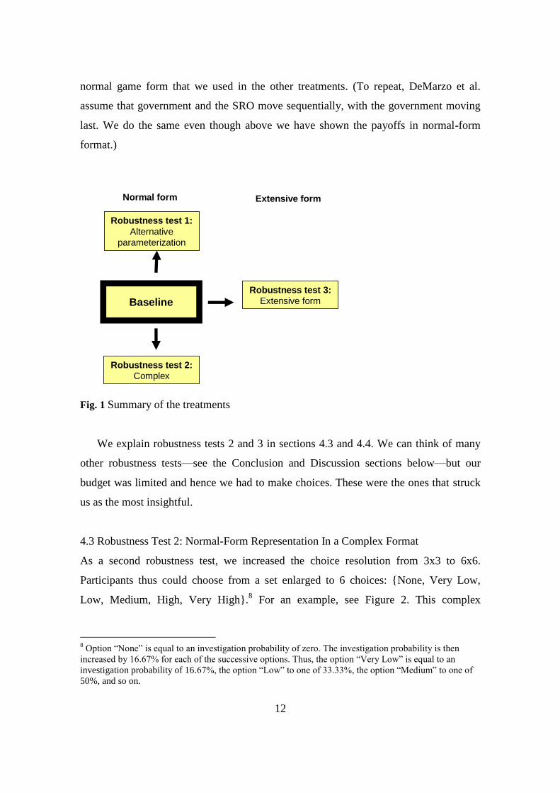
summary of treatments in Figure 1. We also added robustness tests. As a first robustness
test (“Alternative parameterization”), we added a treatment that uses parameterization 6
(“Alternative”) in Table 3. As a second robustness test (“Complex”), we added a
treatment with a higher degree of complexity, and as a third robustness test (“Extensive
form”), we added a treatment with payoffs in the extensive game form rather than in the
12
normal game form that we used in the other treatments. (To repeat, DeMarzo et al.
assume that government and the SRO move sequentially, with the government moving
last. We do the same even though above we have shown the payoffs in normal-form
format.)
Baseline
Robustness test 1:
Alternative
parameterization
Robustness test 2:
Complex
Robustness test 3:
Extensive form
Normal form Extensive form
Fig. 1 Summary of the treatments
We explain robustness tests 2 and 3 in sections 4.3 and 4.4. We can think of many
other robustness tests—see the Conclusion and Discussion sections below—but our
budget was limited and hence we had to make choices. These were the ones that struck
us as the most insightful.
4.3 Robustness Test 2: Normal-Form Representation In a Complex Format
As a second robustness test, we increased the choice resolution from 3x3 to 6x6.
Participants thus could choose from a set enlarged to 6 choices: {None, Very Low,
Low, Medium, High, Very High}.8 For an example, see Figure 2. This complex
8 Option “None” is equal to an investigation probability of zero. The investigation probability is then
increased by 16.67% for each of the successive options. Thus, the option “Very Low” is equal to an
investigation probability of 16.67%, the option “Low” to one of 33.33%, the option “Medium” to one of
50%, and so on.

13
representation has the same order of play and parameterization as the baseline
treatment.
3 6 6
9 9 7
12 9 8
11 4
0
0
13
14 5
05
Row is SROColumn is GOV
1 5 6
7 9 7
13 10 9
8
0
0
17 10
011
6 8 6
11 9 7
12 10 9
9 0
0
0
15
10 0
00
4 7 7
10 10 8
14 11 9
13 4
0
0
15
15 5
06
None
Very Low
Low
Medium
High
Very High
NoneVery Low
Low Medium HighVery High
11 413 13 810
Other
Me
None
Very Low
Low
Medium
High
Very High
15 15 6
13 5 0
4 0 0
10 14
11
9
4
7 10
87
Row is GOVColumn is SRO
10 17 11
13 10 0
8 0 0
7 13
10
9
1
5 9
76
15 10 0
9 0 0
0 0 0
11 12
10
9
6
8 9
76
13 14 5
11 5 0
4 0 0
9 12
9
8
3
6 9
76
Me
NoneVery Low
Low Medium HighVery High
Other
Fig. 2 Presenting the normal-form game to participants in a complex format
Present to SRO (First Mover) Present to GOV (Second Mover)
Other(Move
Second)
Me(Move First)
1 4 6 7 9 7 13 10 9
none low high
none low high none low high none low high
10 14 8 17 10 0 11 0 0
10 14 8 17 10 0 11 0 0
none
low high
none low high none low high none low high
1 4 6 7 9 7 13 10 9
Me(Move
Second)
Other(Move First)
Fig. 3 Presenting the extensive-form game to participants
4.4 Robustness Test 3: Extensive-Form Representation
As a third robustness test, we presented the payoffs in the extensive game form, as this
mode of presentation may be more congruent with the decision process in a sequential
game than the normal-form presentation. The normal-form presentation might make it

14
harder for participants to understand the structure of the sequential decision process. For
an example, see Figure 3.
Table 4 Subgame-perfect Nash equilibria
Nash equilibrium
(SRO, GOV)
Baseline treatment (High, None)
Robustness tests
1. Alternative
parameterization
(normal form)
(Low, Low)
2. Baseline case
complex
(normal form )
(High, None);
(Low, Very Low)
3. Baseline case
(extensive form) (High, None)
Table 5 Sessions, participants, and independent observations
Baseline treatment 2 sessions
48 participants
8 independent observations
Robustness tests
1. Alternative parameterization
(normal form)
2 sessions
48 participants
8 independent observations
2. Baseline case complex
(normal form )
2 sessions
48 participants
8 independent observations
3. Baseline case (extensive form) 1 session
24 participants
4 independent observations
4.5 Nash Equilibria For All Treatments and Experimental Implementation Details
Table 4 shows the subgame-perfect Nash equilibria for our Baseline treatment and the
robustness tests. Due to the rounding of numbers, the Nash equilibria were not identical
in some cases of the robustness test. In the first robustness test (Alternative

15
Parameterization), the Nash equilibrium is (Low, Low). In the second robustness test,
using the complex representation, rounding created other Nash equilibria in addition to
the theoretical one: (Low, Very Low).9 We count these responses as Nash equilibrium
choices in our tests below.
Table 5 gives an overview of our sessions. We ran a total of 7 sessions in December
2011 in the “LEE” experimental lab of the University of Economics in Prague.10
In each
session we had 24 participants make decisions, as SRO or GOV, over 10 rounds.
Following well-documented experimental practice, participants in each session were
divided into 4 groups of 6 to increase the number of truly independent data points. In
each group, 3 participants were randomly assigned the role of GOV and 3 the role of
SRO. Roles were fixed throughout the session. In each round, participants were
randomly matched with a participant playing the other role within their group. Each
session thus resulted in 4 (24÷6) independent observations. We ran a total of 7 sessions
involving 168 participants, generating 28 independent data points. Participants in the
role of SRO made the first choice and their choices were communicated to participants
in the role of GOV with which they were matched. Then participants in the role of GOV
made their choices. We used neutral language in the instructions (reprinted at the end of
this manuscript), and all treatments were implemented using the direct-response
method. Participants earned on average CKZ 360 (≈ €14, ≈ $19, more than four times
the gross hourly average wage in the Czech Republic in 2011) in a session of 50
minutes (including the reading of the instructions).
9 In the complex representation, there is a subgame-perfect Nash equilibrium, (SRO, GOV)=(Low, Very
Low) in addition to the one predicted by theory, (SRO, GOV)=(High, None). The extra Nash equilibrium
is the result of rounding and, as in the case of the Alternative parameterization, the relatively flat payoff
function for GOV. At (Low, Very Low) the SRO has a payoff of 14, and the GOV of 9 (8.5). If numbers
are given with one decimal precision, the option Very Low would be dominated for GOV by option Low,
which results in payoff 9 (9.0). At (Low, Low) the payoff for SRO would be 10, which is lower than the
11 it could secure itself by choosing High. 10
See www.vse-lee.cz. In addition, we ran 6 sessions where players made their choices simultaneously
rather than sequentially. The results of these sessions do not provide evidence related to the theoretical
model of DeMarzo et al. (2005) which has SRO and GOV move sequentially, and we therefore do not
report them here. A detailed account can be found in Van Koten (2014).

16
5 Results
In this section we show the proportion of choices by the participants in the experiments
that are part of a subgame-perfect Nash equilibrium. We interpret the outcome of a high
proportion of choices (or at least a convergence to that outcome) as experimental
corroboration of DeMarzo et al.’s (2005) theoretical model.
5.1 Proportion of Nash equilibrium choices
0.1
.2.3
.4.5
.6.7
.8.9
1
NE
ch
oic
e
1 2 3 4 5 6 7 8 9 10Period
Baseline - paired choice
95% conf. interval/
Fig. 4 Proportion of joint Nash equilibrium choices.
0.1
.2.3
.4.5
.6.7
.8.9
1
NE
ch
oic
e
1 2 3 4 5 6 7 8 9 10Period
Baseline - paired choice
95% conf. interval/

17
Fig. 4 shows the proportion of paired choices that are congruent with a Nash
equilibrium. Initially, choices are far from a Nash equilibrium: typically in less than half
the cases do the pairs make a Nash equilibrium choice. We see, however, a learning
effect. In the last few rounds, paired choices are in all treatments in the range of 50%–
60% . Note that pure chance play would result in success percentages of 11% for paired
choices. However, learning is, less pronounced than we expected, reflecting the fact
that subjects find it difficult to find sequential Nash equilibria. The subjects in the role
of the first-mover (SRO) often make a choice different from the one implied by the
subgame-perfect Nash equilibrium.11
The subjects in the role of second-mover (GOV)
make highly rational choices (see Appendix). When SRO thus makes a first move that is
a Nash equilibrium choice, in most cases the GOV makes a second move that is a Nash
equilibrium as well and visa versa.
0.1
.2.3
.4.5
.6.7
.8.9
1
NE
cho
ice
1 2 3 4 5 6 7 8 9 10Period
Baseline
Robustness tests:
1: Alternative parameterization
2: Complex
3: Extensive
Fig. 5 Proportion of joint Nash equilibrium choices.
11
Our finding of a rather high proportion of dominated choices may be surprising, but is in line with
earlier studies. For example, see Rydval, Ortmann, and Ostatnicky (2009), who report 45% of dominated
choices (where random choice predicts 56% of dominated choices) in simple symmetric, dominance-
solvable guessing games

18
While somewhat alike, the percentage of equilibrium choices in the Alternative
Parameterization treatments (“Alternative”) is higher initially and converges faster to
full equilibrium play than the corresponding percentage in the Baseline. This is likely
the result of the stronger contrast in payoffs for SRO and GOV in the Alternative
parameterization. Recall that the Alternative parameterization has a stronger contrast
because it has a higher success probability than the baseline (50% versus 25% success
probability).
Figure 5 shows the experimental results of our robustness tests (recall that we use an
Alternative parameterization, a more complex format— 6 by 6 instead of 3 by 3—and
an extensive form representation) together with the baseline treatment. The choices for
the baseline treatment are indicated by a thick line with large round markers. The
choices for the treatments of the robustness tests, Alternative parameterization,
Complex representation and Extensive representation are indicated by thin lines with
triangles, diamonds, and squares, respectively. The choices for the Complex treatment
are very much in line with the three treatments that were presented in the simple format
and very close to the average of these three. We conclude that our conclusions are
robust to a different parameterization, a considerable increase in complexity (from 3 to
6 choices for each participant), and the use of an extensive-form representation.
6 Discussion and Conclusion
We have experimentally tested the interesting DeMarzo et al. (2005) model, in
which the authors argue that the mere threat of punishment (government intervention)
might lead to second-best self-regulation. This topic is of importance since many
industries have been trying to rely on self-regulation, which has been theoretically
argued to be incentive-incompatible (Shaked and Sutton 1981; Nunez 2001 2007;
Mysliveček and Ortmann 2010; Ortmann and Svitkova 2010) and has indeed an
empirically questionable track record (e.g., Kleiner 2006). In the light of a lack of
empirical evidence of the efficacy of the threat of government intervention, we
conducted an experimental test of the propositions in DeMarzo et al. (2005) and find

19
that in specific parameterizations and implementation details, the predictions of their
model are borne out.
As always in laboratory tests, a number of extensions and robustness tests suggest
themselves. While we have carefully rationalized the appropriate parameterizations,
there is room for further parametric exploration. We do not believe, however, that
further exploration would lead to substantially different results for rationalizable
parameterizations. As mentioned, an important experimental translation problem is that
an SRO is an organization that is unlikely to be afflicted with social preferences, as
experimental participants might. An obvious robustness test (as a considerable and
growing literature has documented) would therefore be to let teams interact (e.g.,
Charness and Sutter 2012; Cooper and Kagel 2005). In light of the evidence that has
emerged (suggesting that team interaction leads to more play in accordance with
standard game theoretic predictions), we doubt that the essence of our results can be
questioned on those grounds. Other obvious experimental treatments are those
concerning standard experimental manipulations such as financial stakes or the question
of the framing of instructions. Again, we do not believe that this would change our
experimental results significantly (e.g., Rydval and Ortmann 2004).

20
APPENDIX A: Rational individual choices in the sequential game
A1.a The first-mover: SRO
0.1
.2.3
.4.5
.6.7
.8.9
1
Rational choic
e S
RO
in S
EQ
1 2 3 4 5 6 7 8 9 10Period
A1.b The second-mover: GOV
0.1
.2.3
.4.5
.6.7
.8.9
1
Rational choic
e G
OV
in S
EQ
1 2 3 4 5 6 7 8 9 10Period
Fig. A1 Proportion of individual rational choices
In the sequential game SRO is the first-mover and GOV the second-mover. GOV
thus makes its choice knowing the choice of SRO. This allows us to look if GOV makes
profit-maximizing choices, knowing the choice of the choice of the first-mover SRO.
Figure 5 shows the proportion of individual choices that are rational in the game. As
before, the treatments for Baseline and Alternative parameterizations and Extensive
representation are indicated by the round, square, and x-shaped markers, respectively.
The choice of the first-mover, SRO, is regarded as rational if it is the Nash equilibrium
choice. The choice of the second-mover, GOV, is regarded as rational if it is the best
reply to the choice of the participant in the role of SRO he is paired with. The rational
reply for GOV is thus only a Nash equilibrium choice if the paired SRO also made a
Nash equilibrium choice.

21
Figure A1.b shows that GOV makes highly rational choices. Already in the first few
rounds, the proportion of rational choices is mostly above 80%. In the last two rounds,
the proportion of rational choices is above 90% in all treatments. While this may not be
surprising ex-post, earlier studies, such as Rydval et al. (2009) show that very high
proportions of subjects may choose dominated choices in simple guessing games. The
participants in the role of SRO seem to struggle more to make rational choices. Figure
5.a shows that in the first rounds, the percentage of rational choices ranges between
30%–60% and in the last rounds between 50%–90%, indicating learning, most notably
in the Alternative Parameterization (again, due to the larger pay-off contrast between
SRO and GOV in this parameterization). Participants in the role of SRO have a more
difficult task to make a rational choice, as they must deduce their best choices through
backwards induction, assuming a rational response by GOV. It is thus to be expected
that the process of convergence for participants in the role of the first-mover SRO is
slower. It is reassuring that we see convergence for the choices of SRO and that the
rational choices of GOV provide the correct incentive to SRO to learn the rational
responses.
Appendix B: Consolidated instructions
Codes used to indicate the treatment:
Base – Baseline parameterization treatment of 3x3
Alt – Alternative parameterization treatment of 3x3
6x6 – A 6x6 payoff matrix
EXT – Extensive game representation.
A code indicating the start of a text referring to a specific treatment or set of treatments
always starts with “[“ and follows with the codes indicating the specific treatment(s). A
code indicating the end of a text referring to a specific treatment or set of treatments
always ends with the codes indicating the specific treatment(s) and finishes with “]“.
INSTRUCTIONS
Welcome to the experiment!
General rules
Please turn off your mobile phones now.

22
If you have a question, raise your hand and the experimenter will come to your desk to
answer it.
You are not allowed to communicate with other participants during the experiment. If
you violate this rule, you will be asked to leave the experiment and will not be paid (not
even your show-up fee).
Introductory remarks
You are about to participate in an economics experiment. The instructions are simple. If
you follow them carefully, you can earn a substantial amount of money. Your earnings
will be paid to you in cash at the end of the experiment.
The currency in this experiment is called "Experimental Currency Units", or "ECU"s.
At the end of the experiment, we will exchange ECUs for Czech Crowns as indicated
below. Your specific earnings will depend on your choices and the choices of the
participants you will be paired with.
Your exchange rate will be:
[Base
2 Czech Crowns for an ECU.
Base]
[Alt, 3x3, SRO
1.5 Czech Crown for an ECU.
Alt, 3x3, SRO]
[Alt, 3x3, GOV
0.5 Czech Crown for an ECU.
Alt, 3x3, GOV]
This experiment should take at most 60 minutes. There are 10 paid rounds in this
experiment.
You are encouraged to write on these instructions and to highlight what you deem
particularly relevant information.
[Please go to the next page now.]
Group assignment

23
You will always be a member of a group consisting of you and ONE other person in this
room. Group membership is anonymous; you will not know who is in a group with you
and the other person in your group will not know that you are in his or her group.
Group membership is assigned anew in each round, in a random way.
You will be asked to make a series of interactive decisions in this experiment, i.e. your
earnings in each round will depend both on your decision and that of the person
that you are paired with for that round.
In each group one participant will be of Type 1 and the other one will be of Type 2.
The Type 1 participant will make a decision first (“move first”). The choice of the Type
1 participant is then communicated to the Type 2 participant . The Type 2 participant
will make a decision subsequently (“move second“).
The roles of Type 1 and Type 2 are randomly assigned at the beginning of the
experiment and remain the same throughout the experiment. Once the experiment starts,
you will see whether you are Type 1 or Type 2 on your screen in the upper left corner.
Below it you can also see the round. For an example, see Figure 6.
Figure 6
[Please turn over]
Decision Screen
In each round you will be presented with a Decision Screen where you will make a
choice by clicking on one of the
[3x3
three buttons labeled NONE, LOW, or HIGH.
3x3]
[6x6
six buttons labeled using NONE, VERY LOW, LOW, MEDIUM, HIGH, and VERY
HIGH.
6x6]
See the example in Figure 7.

24
Figure 7
[3x3
3x3]
[6x6
6x6]

25
The example in Figure 7 shows how a Type 1 participant, who will move first, will
make a choice. In Figure 8 is shown how a Type 2 participant, who will move second,
will make a choice. As you can see in Figure 8, a Type 2 participant sees the choice that
the Type 1 participant assigned to him or her for that round has made.
Figure 8
[3x3
3x3]
[6x6
26
6x6]
You can see your possible earnings and the possible earnings of the participant assigned
to you for that round in the Earnings Table on the paper with the title “YOUR
EARNINGS TABLE” which you find on your desk.
Your payoffs are in bolded black numbers on yellow background in the upper left
corners of each cell of the Earnings Table. The payoffs of the participant assigned to
you for that round are in blue numbers on a white background in the lower right corner
of each square of the Earnings Table. To repeat, your earnings in each round will
depend both on your choice and that of the person that is assigned to you for that round.
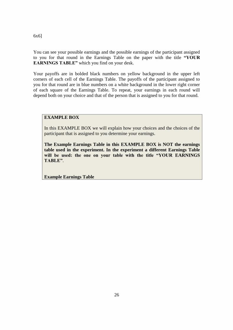
EXAMPLE BOX
In this EXAMPLE BOX we will explain how your choices and the choices of the
participant that is assigned to you determine your earnings.
The Example Earnings Table in this EXAMPLE BOX is NOT the earnings
table used in the experiment. In the experiment a different Earnings Table
will be used: the one on your table with the title “YOUR EARNINGS
TABLE”.
Example Earnings Table
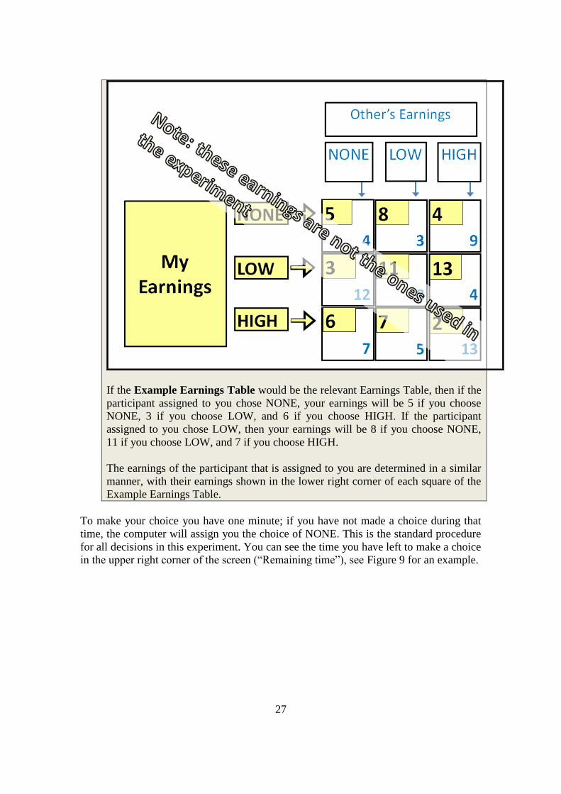
27
If the Example Earnings Table would be the relevant Earnings Table, then if the
participant assigned to you chose NONE, your earnings will be 5 if you choose
NONE, 3 if you choose LOW, and 6 if you choose HIGH. If the participant
assigned to you chose LOW, then your earnings will be 8 if you choose NONE,
11 if you choose LOW, and 7 if you choose HIGH.
The earnings of the participant that is assigned to you are determined in a similar
manner, with their earnings shown in the lower right corner of each square of the
Example Earnings Table.
To make your choice you have one minute; if you have not made a choice during that
time, the computer will assign you the choice of NONE. This is the standard procedure
for all decisions in this experiment. You can see the time you have left to make a choice
in the upper right corner of the screen (“Remaining time”), see Figure 9 for an example.

28
Figure 9
To repeat, Type 1 will make a decision first (“move first”). The choice of Type 1 is then
communicated to Type 2. Type 2 will then make a decision (“move second“).
After all participants have made their decisions, or if one minute has expired, the
computer will calculate your earnings.
Results Screen
You will next see a Results Screen. The Results Screen will show your choice and the
choice of the participant that is assigned to you for that round. The Results Screen will
also show your and the other participants’ earnings.
EXAMPLE BOX
In the example in Figure 3 you and the other participant chose NONE. In the
example in Figure 3 your earnings are thus 5 and that of the other participant are 4
(to repeat: in the experiment a different Earnings Table will be used: the one
on your desk with the title “YOUR EARNINGS TABLE”).

29
You have one minute to inspect the outcomes. (This is the standard time you have for
inspecting results). When you need less time to inspect the outcomes, then click the
NEXT ROUND button. Once all participants have clicked the NEXT ROUND button,
the experiment continues with the next round. Note that the Results Screen will be
visible until all participants have clicked on the NEXT ROUND button.
Do you have any questions at this point?

30
[Base, 3x3, SRO
YOUR EARNINGS TABLE
1 4 6
7 9 7
13 10 9
NONE LOW HIGH
14 8
0
0
10
17 10
011
NONE
LOW
HIGH
Other
Me
Base, 3x3, SRO]
[Base, 3x3, GOV
YOUR EARNINGS TABLE
10 17 11
14 10 0
8 0 0
NONE
LOW
HIGH
LOW HIGH
7 13
10
9
1
4 9
76
NONE
Other
Me
Base, 3x3, GOV ]

31
[Alt, 3x3, SRO
1 19 37
23 40 40
49 46 43
LOW HIGH
52 13
0
0
20
57 31
015
NONE
LOW
HIGH
NONE
Other
Me
Alt, 3x3, SRO]
[Alt, 3x3, GOV
20 57 15
52 31 0
13 0 0
LOW HIGH
23 49
46
43
1
19 40
4037
NONE
LOW
HIGH
NONE
Other
Me
Alt, 3x3, GOV]

32
[Base, 6x6, SRO
3 6 6
9 9 7
12 9 8
11 4
0
0
13
14 5
05
1 5 6
7 9 7
13 10 9
8
0
0
17 10
011
6 8 6
11 9 7
12 10 9
9 0
0
0
15
10 0
00
4 7 7
10 10 8
14 11 9
13 4
0
0
15
15 5
06
NONE
VERY LOW
LOW
MEDIUM
HIGH
VERY HIGH
NONEVERY LOW
LOW MEDIUM HIGHVERY HIGH
11 413 13 810
Other
Me
Base, 6x6, SRO]
[Base, 6x6, GOV
15 15 6
13 5 0
4 0 0
10 14
11
9
4
7 10
87
10 17 11
13 10 0
8 0 0
7 13
10
9
1
5 9
76
15 10 0
9 0 0
0 0 0
11 12
10
9
6
8 9
76
13 14 5
11 5 0
4 0 0
9 12
9
8
3
6 9
76
Me
NONE
VERY LOW
LOW
MEDIUM
HIGH
VERY HIGH
NONEVERY LOW
LOW MEDIUM HIGHVERY HIGH
Other
Base, 6x6, GOV]
[Base, Ext, SRO

33
Other(Move
Second)
Me(Move First)
1 4 6 7 9 7 13 10 9
none low high
none low high none low high none low high
10 14 8 17 10 0 11 0 0
Base, Ext, SRO]
[Base, Ext, GOV
10 14 8 17 10 0 11 0 0
none
low high
none low high none low high none low high
1 4 6 7 9 7 13 10 9
Me(Move
Second)
Other(Move First)
Base, Ext, GOV]

34
References
Charness, G. and Sutter, M. (2012). Groups Make Better Self-Interested Decisions,
Journal of Economic Perspectives, 26, 157 – 176.
Cooper, D. J. and Kagel, J. H. (2005). Are Two Heads Better Than One? Team Versus
Individual Play in Signaling Games, American Economic Review, 95, 477 – 509.
DeMarzo, P. M., Fishman, M. J., and Hagerty, K. M. (2005). Self-Regulation and
Government Oversight, Review of Economic Studies, 72, 687 – 706.
Eckel, C. and Lutz, N. (2003). Introduction: What Role Can Experiments Play in
Research on Regulation? Journal of Regulatory Economics 23(2), 103 – 107.
Gehrig, T. and Jost, P-J. (1995). Quacks, Lemons, and Self Regulation: A Welfare
Analysis. Journal of Regulatory Economics 7, 309 – 325.
Hilary, G. and Lennox, C. (2005). The Credibility of Self-Regulation: Evidence from
the Accounting Profession's Peer Review Program, Journal of Accounting and
Economics, 40, 211 – 229.
Hinloopen, J., Müller, W., and Normann, H. (2012). Output Commitment through
Product Bundling: Experimental Evidence, Tinbergen Institute Discussion Paper
No. 11–170/1.
Holt, C. and Laury, S. K. (2002). Risk Aversion and Incentive Effects, The American
Economic Review, 92, 1644 – 1655.
Huck, S., Müller, W., and Normann, H. (2001). Stackelberg Beats Cournot: On
Collusion and Efficiency in Experimental Markets, Economic Journal, 111, 749 –
765.
Kleiner, M. M. (2006). Licensing Occupations: Ensuring Quality or Restricting
Competition? (W. E. Upjohn Institute for Employment Research).
List, J. A. (2006). The Behavioralist Meets the Market: Measuring Social Preferences
and Reputation Effects in Actual Transactions, Journal of Political Economy, 114, 1
– 37.
Maute, J. L. (2008). Bar Associations, Self-Regulation and Consumer Protection:
Whither Thou Goest?, Journal of the Professional Lawyer, 53 – 85.
Nunez , J. (2001). A Model of Self-Regulation, Economics Letters, 74, 91 – 97.
35
Nunez, J. (2007). Can Self-Regulation work? A Story of Corruption, Impunity and
Cover-up, Journal of Regulatory Economics, 31, 209 – 233.
Ortmann, A. and Mysliveček, J. (2010). Certification and Self-Regulation of Non-
Profits, and the Institutional Choice Between Them, in Seaman, B. and Young, D.
(eds) Handbook of Nonprofit Economics and Management (Cheltanham: Edward
Elgar Publishing Company).
Ortmann, A. and Svitkova, K. (2010). Do Self-Regulation Clubs Work? Some Evidence
from Europe and Some Caveats From Economic Theory, in Gugerty, M. K. and
Prakash, A. (eds) Voluntary Regulation of NGOs and Non-Profits: An
Accountability Club Framework (Cambridge: Cambridge University Press).
Rees, J. V. (1997). The Development of Communitarian Regulation in the Chemical
Industry, Law Policy, 17, 477 – 528.
Rydval, O. and Ortmann, A. (2004). How Financial Incentives and Cognitive Abilities
Affect Task Performance in Laboratory Settings: An Illustration, Economics Letters,
85, 315 – 320.
Shaked, A. and Sutton, J. (1981). The Self-Regulating Profession, The Review of
Economic Studies, 48, 217 – 234.
Sidel, M. (2005). The Guardians Guarding Themselves: A Comparative Perspective on
Nonprofit Self-Regulation, Kent Law Review, 80, 803 – 835.
Studdert, D. M., Mello, M. M., and Brennan, T. A. (2004). Financial Conflicts of
Interest in Physicians’ Relationship with the Pharmaceutical Industry: Self-
Regulation in the Shadow of Federal Prosecution, New England Journal of
Medicine, 351, 1891 – 1900.
Van Koten (mimeo). Self-regulation under the shadow of governmental oversight:
blossom or perish?

Working Paper Series ISSN 1211-3298 Registration No. (Ministry of Culture): E 19443 Individual researchers, as well as the on-line and printed versions of the CERGE-EI Working Papers (including their dissemination) were supported from institutional support RVO 67985998 from Economics Institute of the ASCR, v. v. i. Specific research support and/or other grants the researchers/publications benefited from are acknowledged at the beginning of the Paper. (c) Silvester Van Koten and Andreas Ortmann, 2014 All rights reserved. No part of this publication may be reproduced, stored in a retrieval system or transmitted in any form or by any means, electronic, mechanical or photocopying, recording, or otherwise without the prior permission of the publisher. Published by Charles University in Prague, Center for Economic Research and Graduate Education (CERGE) and Economics Institute of the ASCR, v. v. i. (EI) CERGE-EI, Politických vězňů 7, 111 21 Prague 1, tel.: +420 224 005 153, Czech Republic. Printed by CERGE-EI, Prague Subscription: CERGE-EI homepage: http://www.cerge-ei.cz Phone: + 420 224 005 153 Email: [email protected] Web: http://www.cerge-ei.cz Editor: Marek Kapička The paper is available online at http://www.cerge-ei.cz/publications/working_papers/. ISBN 978-80-7343-324-6 (Univerzita Karlova. Centrum pro ekonomický výzkum a doktorské studium) ISBN 978-80-7344-316-0 (Akademie věd České republiky. Národohospodářský ústav)