Embed Size (px)
Citation preview
Acta Applicandae Mathematicae58: 189–215, 1999.© 1999Kluwer Academic Publishers. Printed in the Netherlands.
189
On the Accuracy of Gaussian Approximation inHilbert Space
S. V. NAGAEVSobolev Institute of Mathematics, Koptjug prospekt 4, 630090 Novosibirsk, Russia.e-mail: [email protected]
V. I. CHEBOTAREVComputer Centre of Far East Branch of Russian Academy of Science, Tikhookeanskaya str. 153,680042 Khabarovsk, Russia. e-mail: [email protected]
(Received: 28 August 1999)
Abstract. The bound on remainder term in CLT for a sum of independent random variables takingvalues in Hilbert space is obtained. This bound sharpens the result due to Bentkus and Götze.
Mathematics Subject Classification (1991):60B12.
Key words: Hilbert space, Gaussian approximation, covariance operator, random vector, eigenval-ues, Borel function, inner product.
1. Introduction
LetH be a separable Hilbert space with the norm|· | and the inner product(· , · ),X,X1,X2, . . . beH -valued i.i.d. random variables with the covariance operatorT
andEX = 0. Denote byσ 21 > σ 2
2 > · · · the eigenvalues ofT , and bye1, e2, . . . thecorresponding eigenvectors. Put
3l =l∏
j=1
σ 2j , σ 2 = E|X|2, βµ = E|X|µ,
0µ,l = βµσµ/3µ/l
l .
Let8(· ) be the Gaussian distribution with the covariance operatorT . Denote
Sn = n−1/2n∑j=1
Xj .
LetB(a, r) be the ball{x : x ∈ H, |x − a| < r}. Denote
1n(a; r) =∣∣P(Sn ∈ B(a, r))−8(B(a, r))∣∣, 1n(a) = sup
r>01n(a; r).
190 S. V. NAGAEV AND V. I. CHEBOTAREV
It follows from the results of Bentkus and Götze [4] that
1n(α) <C
n
(β4
σ 4+ β
23
σ 6
)with
C 6 exp{cσ 2/σ 2
13
},
wherec is an absolute constant.Let us formulate our result in this direction. Denote
Ll = max16j6l
β3j
σ 3j
,
where
β3,j = E∣∣(X, ej )∣∣3.
THEOREM. There exists an absolute constantc such that
1n(0) <c
n
(04,13+ 02
3,13+(σ 2
31/99
)2
L29
). (1.1)
Using (1.1), we can obtain simpler bounds.
EXAMPLE. Notice that
Ll 6β3
σ 3l
.
Therefore, we may replace the third summand in the bound (1.1) by(σ 2β3
σ 293
29
)2
<σ 11β4
31/215
.
On the other hand,
04,13 <β4σ
11
31/215
, 023,13 <
β4σ11
31/215
.
As a result, we obtain the bound
1n(0) <cβ4σ
11
n31/215
.
The latter is much simpler than (1.1) but, of course, rougher.
ON THE ACCURACY OF GAUSSIAN APPROXIMATION IN HILBERT SPACE 191
We shall use the following notations:X′ – independent copy ofX,Xs = X−X′,X = X − EX. Let
B(x;L) = E[(Zs, x)2; |Z| ∨ |Z′| 6 L],
whereZ is an arbitraryH -valued random variable, andσ 2j (L) > σ 2
j+1(L), j =1,∞, are the eigenvalues ofB(x;L).
Denote
3l(L) =l∏1
σ 2k (L), δ2
l (L) =L2
32/ ll (L)
l∑i
σ 2j (L), f Yx (t) = Eeit (Y,x).
We shall use the notationI (A) to denote the indicator of the setA. The symbolsc(l) indicates a constant depending onl. Absolute constants will be denoted byc.
In the present paper, the results and the methods of the papers [1 – 7] are ap-plied. On the other hand, some new ideas are used. In this connection, we draw thereader’s attention to the key Lemmas 3.1, 3.3–3.6, 3.12, 3.13. It should be noticedthat we do not use the specific methods of the number theory in contrast with [4].
2. Bounds on Characteristic Functions in the Neighborhood of Zero
LetX,X1, . . . , Xn, . . . be a sequence of i.i.d.H -valued random vectors. In contrastto the introduction, we do not suppose in this section thatEX = 0. We shall usenotationsUk1,k2 =
∑k2k1Xj , Um = U1,m.
LEMMA 2.1. For every1< m < n, L > 0, t ∈ RE[∣∣f Um+1,n
Usm(2t)
∣∣; |Um| ∨ |U ′m| < √3/8|t|L]6 c(l)
[(1+3l(L)
(|t|√m(n−m))l)−1+(δl(L)√m
)l]. (2.1)
LEMMA 2.2. LetX andY be independentH -valued random vectors. Then, foreveryr > 0, a ∈ H , t ∈ R,∣∣E exp
{it|X + Y − a|2}∣∣ < P(|X| > r) sup
b∈H
∣∣E exp{it|Y − b|2}∣∣ +
+E1/2[∣∣f YXs (2t)∣∣; |X| ∨ |X′| 6 r]. (2.2)
Both lemmas are proved in [7].Denotec0 =
√3/8.
LEMMA 2.3. Let
B−1/2n 6 |t| 6 c0
2σL(2.3)
192 S. V. NAGAEV AND V. I. CHEBOTAREV
and{li}k1 be any sequence such that
16 li 6c0
2σL|t| , (2.4)
k∑i
l−2i < 2
( |t|σLc0
)2
n. (2.5)
Then
supa∈H
∣∣E exp{it|Un − a|2
}∣∣ < c(l)|t|l/2D(l) k∑i
ll/2j /4
j + 4−k, (2.6)
where
D(l) = (σL)l/2(B−l/2+ (σL)l/2)/31/2l (L). (2.7)
Proof.Define the sequence{mi}k1 by the formula
mi =[(c0/2liσL|t|
)2]. (2.8)
Notice that in view of (2.4)mi > 1. Letµj =∑j
1mi. Denote
qj (t) = supa∈H
∣∣E exp{it|Uµj+1,n − a|2
}∣∣.Putting in Lemma 2.2r = 2σ
√mj , X = Uµj−1,µj − EUµj−1,µj Y = Uµj+1,n −
EUµj+1,n, we obtain the inequalities
qj−1(t) 61
4qj (t)+Qj, j = 1, . . . , k, (2.9)
where
Qj = E{∣∣f Uµj+1,n
Usmj(2t)
∣∣; ∣∣Umj ∣∣ ∨ ∣∣U ′mj ∣∣ < 2σ√mj
}; U = U − EU.
We used here the boundP(|x| > r) < E|X|2/r2 = 14 and the equalityUµj−1+1,µj −
EUµj−1+1,µjd= Umj − EUmj .
Since by (2.4) and (2.8)r <√
3/8|t|L, we may apply Lemma 2.1 to estimateQi. As a result we have
Qi < c(l)(ai + bi), (2.10)
where
ai =(1+3l(L)
(|t|√mi(n− µi))l)−1/2,
bi =(δl(L)√mi
)l/2.
ON THE ACCURACY OF GAUSSIAN APPROXIMATION IN HILBERT SPACE 193
In view of (2.1)
δ2l (L) <
2L2σ 2
32/ ll (L)
.
Therefore
bi <
(2Lσ
31/ ll (L)
√mi
)l/2< c(l)(li |t|)l/2bl , (2.11)
where
bl =(Lσ/3
1/2ll
)l. (2.12)
By (2.5) and (2.8)
µi < µk 6 n/2. (2.13)
Hence, taking into account (2.3) and (2.8), we deduce
ai <
(cLσ li
31/ ll (L)
√n
)l/2< c(l)(lit)
l/2al , (2.14)
where
al =(
Lσ
B31/ ll (L)
)l/2. (2.15)
It follows from (2.10), (2.11), (2.14), that
qi−1(t) <1
4qi(t)+ c(l)(al + bl )(li|t|)l/2.
Subsequently applying this inequality fori = 1, . . . , k we conclude that
q0(t) <1
4kqk(t)+ c(l)|t|l/2(al + bl)
k∑1
ll/2j
/4j .
It remains to use the trivial boundqk(t) 6 1 and to insert insteadal and bl theexpressions (2.15) and (2.12).
LEMMA 2.4. If
Bn−1/2 6 |t| 6 c0
8σL, (2.16)
then
supa∈H
∣∣ exp{it|Un − a|2
}∣∣ < c(l)D(l)|t|l/2. (2.17)
194 S. V. NAGAEV AND V. I. CHEBOTAREV
Proof.Put
ll/2i = 4i/2
(2/42/ l − 1
)l/4(c0/2|t|σL√n
)l/2+ 1, (2.18)
k0 = max{i: li 6
c0
2δL|t|}. (2.19)
Then
l2i 42i/ l2/
(42/ l − 1
)(c0/2|t|σL
√n)2.
Hence∞∑1
l−2i < 2
( |t|δLc0
)2
n. (2.20)
Further, by (2.18)
∞∑1
ll/2i
4i<
(c0
2|t|σL√n)l/2+ 1. (2.21)
According to (2.19),
lk0 >c0
2σL|t| − 1. (2.22)
It follows from (2.16), (2.18) and (2.22) that
c0
4σL|t| <c0
2σL|t| − 2< lk0 < 4k0/ l
(2
42/ l− 1
)1/2c0
2|t|σL√n.
Hence
4−k0 <
(2√
2
42/ l − 1
)l/2n−l/2. (2.23)
Puttingk = k0 in Lemma 2.3 and taking into account (2.19), (2.20) and (2.23) weobtain the bound
supa∈H
∣∣E exp{it|Un − a|
}∣∣ < c(l)
(|t|l/2D(l)
((1
2|t|σL√n)l/2+ 1
)+ n−l/2
)< c1(l)
(|t|l/2D(l)+ n−l/2) < c2(l)|t|l/2D(l).This completes the proof of Lemma 2.4.
LEMMA 2.5. If |t| < c0(2l/2Lσ(L)√
2n)−1, then
Ea∈H
exp{it|Un − a|2
}<
c(l)√1+3l(L)(|t|n)l
. (2.24)
ON THE ACCURACY OF GAUSSIAN APPROXIMATION IN HILBERT SPACE 195
3. Some Preparation Bounds
LEMMA 3.1. LetAk be the set of vectorsa = (a1, a2, . . . , aN ) such that
|aj | < λj/2N, j 6= k, λk < |ak| < (1+ ε)λk. (3.1)
Then, for everyx = (x1, x2, . . . , xN ),
N∑1
infa∈Ak
(x, a)2 >1
4N
N∑1
λ2jx
2j , (3.2)
maxk
supa∈Ak
(x, a)2 < N(1+ ε)2N∑1
λ2jx
2j . (3.3)
Proof.Let k be fixed and
λk|xk| > λj |xj |, j 6= k. (3.4)
Then by (3.1), for everya ∈ Ak,
|(x, a)| > |xkak| −∑j 6=k|xjaj | > λk|xk| − 1
2N
∑j 6=k
λj |xj | > λk|xk|/2.
Hence,
∑j
infa∈Aj
(x, a)2 > infa∈Ak
(x, a)2 > λ2kx
2k /4>
1
4N
N∑1
λ2jx
2j .
Obviously, for everyx there existsk for which (3.4) holds. It means that (3.2) isvalid for everyx.
Now prove (3.3). By (3.1) for everya ∈⋃N1 Aj
|(x, a)| < (1+ ε)N∑1
λk|xk|.
On the other hand,(N∑1
λk|xk|)2
< N
N∑1
λ2kx
2k .
Thus
supj
supa∈Aj
(x, a)2 < (1+ ε)2NN∑1
λ2kx
2k .
This completes the proof.
196 S. V. NAGAEV AND V. I. CHEBOTAREV
The following inequality is proved in [6].
LEMMA 3.2. Let random variableξ > 0 andF(r) be the distribution ofξ . IfF(r) < Qrl for r > ε > 0, then
E exp{− ξ2f 2
}<(c(l)t−l + rl)Q,
wherec(l) 6 0(l/2+ 1), 0(p) being the Euler function.
LEMMA 3.3. Let F be the discrete positive measure concentrated on the unionof two finite disjoint setsA = (x1, x2, . . . , xm) andB = (y1, . . . , ym). Then thereexists the nonnegative matrixεij , i = 1,m, j = 1, n, such thatF is represented asthe mixture
F =m∑i=1
n∑j=1
εijFij , (3.5)
whereFij are two-point probability measures,
Fij (xi) = a
a + 1, Fij (yj ) = 1
a + 1, a = F(A)
F(B),
and, in addition,∑i,j
εijFij (xi) = F(A),∑i,j
εijFij (yj ) = F(B).
Proof.Denotepi = F(xi), qj = F(yj ). Without loss of generalityp1 > p2 >· · · > pm, q1 > q2 > · · · > qn. If p1 < aq1, then putε11 = (a + 1)q1. As a result
F = ε11F11+ F1, (3.6)
whereF1(x1) = 0, F1(y1) = q1 − ap1, F1(xi) = F(xi), i > 1, F1(yj ) = F(yj ),j > 1. SoF1 is concentrated on the union of the setsA1 := (x2, x3, . . . , xm) andB.
If p1 > aq1, thenε11 = (a + 1)qi , F1(x1) = p1 − q1/a, F1(y1) = 0,F1(xi) =F(xi), i > 1,F1(yj ) = f (yj ), j > 1, i.e.,F1 in (3.6) is concentrated on theA∪B1,B1 = (y2, . . . , ym). In the casep1 = aq1 we haveF1(x1) = F1(y1) = 0 andF1 isconcentrated onA1 ∪ B1. Repeating this procedure at mostm + n steps we cometo representation (3.5).
LEMMA 3.4. Let random vectorX take two valuesx1 andx2, x1 6= x2, P(X =x1) = p, P(X = x2) = q. Then
E{((X +X′)s, y)2
/Xs = (Xs)′ = 0} = 8p2q2
(p2+ q2)2(x1− x2, y)
2, (3.7)
E{((X +X′)s, y)2
/Xs = (Xs)′ = x2 − x1} = 0. (3.7′)
ON THE ACCURACY OF GAUSSIAN APPROXIMATION IN HILBERT SPACE 197
Proof. It is easily seen that
P(X +X′ = 2x1/X
s = 0) = p2
p2+ q2,
P(X +X′ = 2x2/X
s = 0) = q2
p2+ q2.
Therefore
P((X +X′)s = 2(x1 − x2) /X
s = (Xs)′ = 0)
= P((X +X′)s = 2(x2 − x1) /X
s = (Xs)′ = 0)
= p2q2
(p2+ q2)2. (3.8)
Obviously (3.8) implies equality (3.7). It is sufficient to remark thatXs =(Xs)′ = x2 − x1 implies(X +X′)s = 0 in order to prove (3.7′).
LEMMA 3.5. Let (Xk, Yk), k = 1, n, be the sequence of independent randomvariables taking values inH ×H . Then, for every Borel functionϕ(· ) onH ,
En∏1
∣∣E(ϕ(Xk)/Yk)∣∣ = n∏1
E∣∣E(ϕ(Xk)/Yk)∣∣.
Proof.Random variables
ξk =∣∣E(ϕ(Xk)/Yk)∣∣
are independent. Therefore
En∏1
ξk =n∏1
Eξk.
Call the random vectorX′ by a conditionally independent copy ofX relative toσ -algebraB if, for every Borel functionsϕ1(· ) andϕ2(· ),
E(ϕ1(X)ϕ2(X
′)/B) = E
(ϕ1(X)/B
)E(ϕ2(X)/B
).
Let the sequence(Xk, Yk) be the same as in Lemma 3.5. As above, we use thenotationVk,m =∑m
k Xj , V k,m = Vk,m − EVk,m, Vm = V1,m.Let Bk,m be σ -algebra generated by random variablesYj , j = k,m, Bm =
B1,m. Denote
ϕk(t;Bk) = supb∈H
∣∣E{exp(it|Vk − b|2)/Bk
}∣∣,ϕk(t) = Eϕk(t;Bk),
198 S. V. NAGAEV AND V. I. CHEBOTAREV
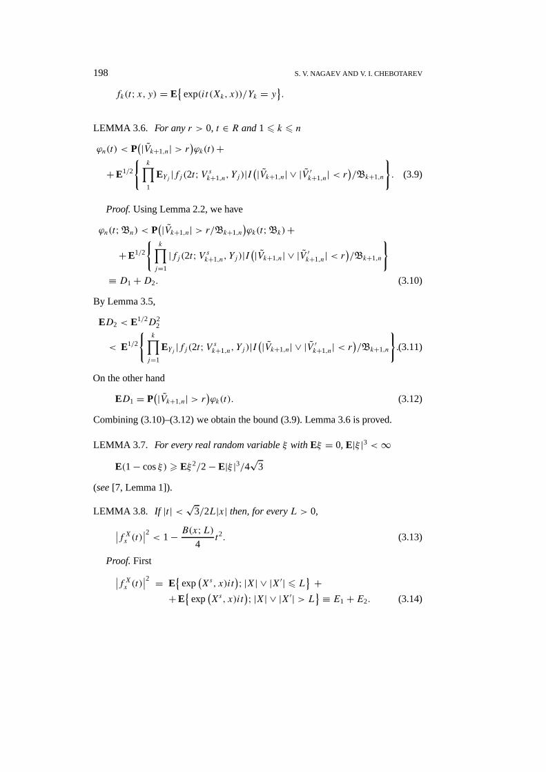
fk(t; x, y) = E{
exp(it (Xk, x))/Yk = y}.
LEMMA 3.6. For anyr > 0, t ∈ R and16 k 6 n
ϕn(t) < P(|Vk+1,n| > r
)ϕk(t)+
+E1/2
{k∏1
EYj |fj(2t;V sk+1,n, Yj )|I
(|Vk+1,n| ∨ |V ′k+1,n| < r)/Bk+1,n
}. (3.9)
Proof.Using Lemma 2.2, we have
ϕn(t;Bn) < P(|Vk+1,n| > r/Bk+1,n
)ϕk(t;Bk)+
+E1/2
{k∏j=1
|fj(2t;V sk+1,n, Yj )|I
(|Vk+1,n| ∨ |V ′k+1,n| < r)/Bk+1,n
}≡ D1+D2. (3.10)
By Lemma 3.5,
ED2 < E1/2D22
< E1/2
{k∏j=1
EYj |fj(2t;V sk+1,n, Yj )|I
(|Vk+1,n| ∨ |V ′k+1,n| < r)/Bk+1,n
}.(3.11)
On the other hand
ED1 = P(|Vk+1,n| > r
)ϕk(t). (3.12)
Combining (3.10)–(3.12) we obtain the bound (3.9). Lemma 3.6 is proved.
LEMMA 3.7. For every real random variableξ with Eξ = 0, E|ξ |3 <∞E(1− cosξ) > Eξ2/2− E|ξ |3/4√3
(see[7, Lemma 1]).
LEMMA 3.8. If |t| < √3/2L|x| then, for everyL > 0,∣∣f Xx (t)∣∣2 < 1− B(x;L)4
t2. (3.13)
Proof.First∣∣f Xx (t)∣∣2 = E{
exp(Xs, x)it
); |X| ∨ |X′| 6 L} ++E
{exp
(Xs, x)it
); |X| ∨ |X′| > L} ≡ E1 + E2. (3.14)
ON THE ACCURACY OF GAUSSIAN APPROXIMATION IN HILBERT SPACE 199
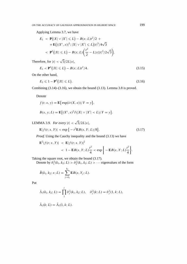
Applying Lemma 3.7, we have
E1 < P(|X| ∨ |X′| 6 L)− B(x;L)t2/2 ++E
(|(Xs, x)|3; |X| ∨ |X′| 6 L)|t|3/4√3
< P2(|X| 6 L)− B(x;L)( t22− L|x||t|3/2√3
).
Therefore, for|t| < √3/2L|x|,E1 < P2(|X| 6 L)− B(x;L)t2/4. (3.15)
On the other hand,
E2 6 1− P2(|X| 6 L). (3.16)
Combining (3.14)–(3.16), we obtain the bound (3.13). Lemma 3.8 is proved.
Denote
f (t; x, y) = E{
exp(it (X, x))/Y = y},B(x, y;L) = E
{(Xs, x)2I (|X| ∨ |X′| < L)/Y = y}.
LEMMA 3.9. For every|t| < √3/2L|x|,E|f (t; x, Y )| < exp
{− t2EB(x, Y ;L)/8}. (3.17)
Proof.Using the Cauchy inequality and the bound (3.13) we have
E2|f (t; x, Y )| < E|f (t; x, Y )|2
< 1− EB(x, Y ;L)t2
4< exp
{− EB(x, Y ;L)t
2
4
}.
Taking the square root, we obtain the bound (3.17).Denote byσ 2
1 (k1, k2;L) > σ 22 (k1, k2;L) > · · · eigenvalues of the form
B(k1, k2; x;L) =k2∑j=k1
EB(x, Yj ;L).
Put
3l(k1, k2;L) =l∏1
σ 2j (k1, k2;L), σ 2
j (k;L) = σ 2j (1, k;L),
3l(k;L) = 3l(1, k;L).
200 S. V. NAGAEV AND V. I. CHEBOTAREV
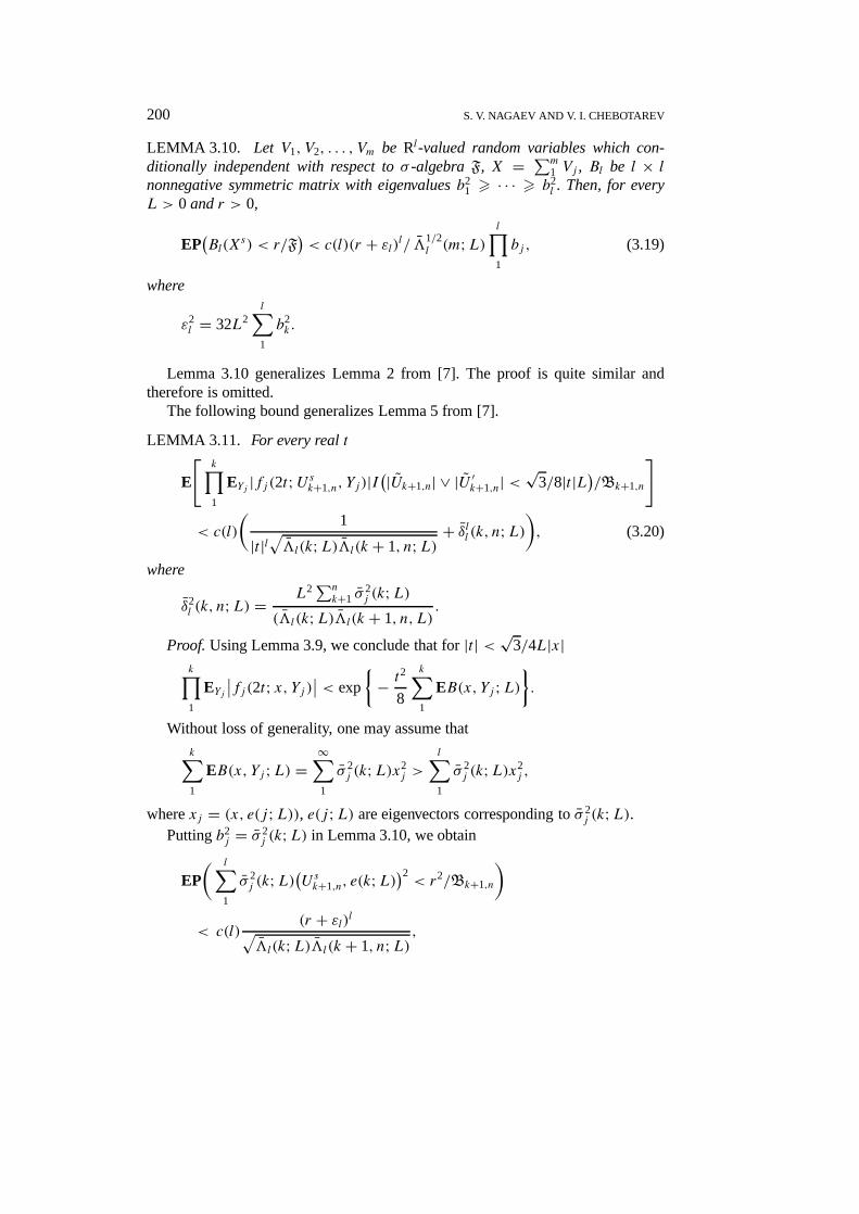
LEMMA 3.10. Let V1, V2, . . . , Vm be Rl-valued random variables which con-ditionally independent with respect toσ -algebra F, X = ∑m
1 Vj , Bl be l × lnonnegative symmetric matrix with eigenvaluesb2
1 > · · · > b2l . Then, for every
L > 0 andr > 0,
EP(Bl(X
s) < r/F)< c(l)(r + εl)l/ 31/2
l (m;L)l∏1
bj , (3.19)
where
ε2l = 32L2
l∑1
b2k .
Lemma 3.10 generalizes Lemma 2 from [7]. The proof is quite similar andtherefore is omitted.
The following bound generalizes Lemma 5 from [7].
LEMMA 3.11. For every realt
E
[k∏1
EYj |fj(2t;Usk+1,n, Yj )|I
(|Uk+1,n| ∨ |U ′k+1,n| <√
3/8|t|L)/Bk+1,n
]
< c(l)
(1
|t|l√3l(k;L)3l(k + 1, n;L)
+ δll (k, n;L)), (3.20)
where
δ2l (k, n;L) =
L2∑n
k+1 σ2j (k;L)
(3l(k;L)3l(k + 1, n, L).
Proof.Using Lemma 3.9, we conclude that for|t| < √3/4L|x|k∏1
EYj∣∣fj(2t; x, Yj )∣∣ < exp
{− t
2
8
k∑1
EB(x, Yj ;L)}.
Without loss of generality, one may assume that
k∑1
EB(x, Yj ;L) =∞∑1
σ 2j (k;L)x2
j >
l∑1
σ 2j (k;L)x2
j ,
wherexj = (x, e(j;L)), e(j;L) are eigenvectors corresponding toσ 2j (k;L).
Puttingb2j = σ 2
j (k;L) in Lemma 3.10, we obtain
EP( l∑
1
σ 2j (k;L)
(Usk+1,n, e(k;L)
)2< r2/Bk+1,n
)< c(l)
(r + εl)l√3l(k;L)3l(k + 1, n;L)
,
ON THE ACCURACY OF GAUSSIAN APPROXIMATION IN HILBERT SPACE 201
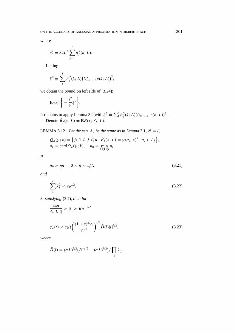
where
ε2l = 32L2
l∑j=1
σ 2j (k;L).
Letting
ξ2 =l∑1
σ 2j (k;L)
(Usk+1,n, e(k;L)
)2,
we obtain the bound on left side of (3.24):
E exp
{− t
2
8ξ2
}.
It remains to apply Lemma 3.2 withξ2 =∑l1 σ
2j (k;L)(Uk+1,n, e(k;L))2.
DenoteBj (x;L) = EB(x, Yj ;L).
LEMMA 3.12. Let the setsAk be the same as in Lemma3.1,N = l,Qn(γ ; k) =
{j : 16 j 6 n, Bj (x;L) = γ (aj, x)2, aj ∈ Ak
},
nk = card�n(γ ; k), n0 = min16k6l
nk.
If
n0 > ηn, 0< η < 1/l, (3.21)
and
l∑1
λ2i < γ1σ
2, (3.22)
λi satisfying(3.7), then for
c0n
4σL|t| > |t| > Bn−1/2
ϕn(t) < c(l)
((1+ ε)2γ1
γ η2
)l/4D(l)|t|l/2, (3.23)
where
D(l) = (σL)l/2(B−l/2+ (σL)l/2)/ l∏1
λj .
202 S. V. NAGAEV AND V. I. CHEBOTAREV
Proof.Let li be defined by (2.17) and, in addition,
li 6c0η
4σL|t| . (3.24)
Further letmi satisfy (2.8) andµj =∑j
1mi.Denote
mik = card(�n(γ ; k) ∩ {j : µi < j 6 µi+1}
).
Notice thatϕn(t) does not depend on the order of summandsXi .Therefore, taking into acount (3.21), we may assume without loss of generality
thatmik > [ηmi], k = 1, l. It follows from (2.7) and (3.24) that
mi > 2/η.
Hence,[ηmi] > 2. It means in turn that[ηmi] > ηmi/2, i.e.,
mik > ηmi, k = 1, l. (3.25)
Denote
qi (t) = ϕn−µi (t).Takingn− µi−1 instead ofn in Lemma 3.6 and puttingk = n− µi , r = 2σ
√mi ,
we conclude that
qi−1 <1
4qi + Qi, (3.26)
where
Qi = E1/2n−µi∏j=1
EYj∣∣fj(2t;Uµi−1+1,µi , Yj )
∣∣,(∣∣Uµi−1+1,µi
∣∣ ∨ ∣∣Uµi−1+1,µi
∣∣ < 2σ√mi/Bµi−1,µi
).
Applying Lemma 3.12, we have
Qi < c(l)
[1
|t|l/23l/4l (µi−1, µi;L)3l/4
l (n− µi;L)+ δl/2(n− µi;L)
]. (3.27)
Here we took into account that by (2.17),li > 1 and, consequently,σ√mi <√
3/8|t|L.Using (3.25) and Lemma 3.1, we get the inequalities
γ ηmi
2
l∑1
λ2jx
2j <
µi∑µi−1+1
Bj (x;L) < γmi(1+ ε)2l∑1
λ2jx
2j .
ON THE ACCURACY OF GAUSSIAN APPROXIMATION IN HILBERT SPACE 203
Hence
1
2γ ηmiλ
2j < σ
2j (µi−1 + 1, µi;L) < γmil(1+ ε)2λ2
j , j = 1, l.
Consequently(γ ηmi
2
)l l∏1
λ2j < 3l
(µi−1 + 1, µi;L
)< (γmil)
l(1+ ε)2l∏1
λ2j . (3.28)
Similarly
1
2γ η(n− µi)λ2
j < σ 2j (n− µi;L) < γ (n− µi)l(1+ ε)2λ2
j , (3.29)
(γ η(n− µi)
2
)l< 3l(n− µi;L) <
(γ l(n− µi)
)l(1+ ε)2l
l∏1
λ2j . (3.30)
It follows from (3.28)–(3.30) that
δ2(n− µi;L) < c(l)(1+ ε)2L2∑l
1 λ2j
γ η2∏l
1 λ4jmi
. (3.31)
combining (3.27), (3.28), (3.30) and (3.31) we get
Qi < c(l)(ai + bi), (3.32)
where
ai = 1
|t|l/2ml/4i (n− µi)l/4(γ η)l/2∏l
1 λj,
bi =((1+ ε)2L2∑l
1 λ2i
miγ η2∏l
1λ4j
)l/4.
It follows from (2.7), (2.12) and (2.15)
ai < c
(σLli
γ η√n
)l/2( l∏1
λj
)−1
< c(l)(γ η)−l/2(lit)l/2al, (3.33)
where
al = (Lσ/B)l/2(
l∏1
λj
)−1
.
204 S. V. NAGAEV AND V. I. CHEBOTAREV
Further, by (2.7) and (3.26)
bi < c(l)(1+ ε)2γ1
γ η2(li |t|)l/2bl , (3.34)
where
bl = (σL)l/l∏1
λj .
Combining (3.26) and (3.32)–(3.34), we obtain the inequality
qi−1 <1
4qi + c(l)
(al + bl
)(li |t|)l/2.
Hence, by (3.24),
q0 <1
4k0+ c(l)|t|l/2(al + bl),
where
k0 = max
{k: lk 6
c0η
4σL|t|}.
Subsequent arguments coincide with those proving Lemma 2.4.
LEMMA 3.13. Let the conditions of Lemma3.13hold and
|t| < c0/2l/2σL
√n.
Then
ϕn(t) < c(l)
(γ1(1+ ε)2(γ η)2
)l/4(nt
l∏1
λj
)−l/2.
4. Estimation of a Characteristic Function in the Neighborhood of the Unit
Let X1,X2, . . . , Xn, . . . be independent random variables, taking values inH ,Un = ∑n
1Xj . DenoteX0j = Xj + X′j , U0
n =∑n
1X0j . Let An be aσ -algebra
generated by random variableXsj , j = 1, n.
Define
9n(t; τ ; a) =∣∣E exp
{it|Un − a|
}∣∣ ∣∣E exp{i(t + τ)|Un − a|2
}∣∣,9(τ ; b;An) =
∣∣E{exp{iτ∣∣U0
n − b∣∣2}/An
}∣∣.
ON THE ACCURACY OF GAUSSIAN APPROXIMATION IN HILBERT SPACE 205
LEMMA 4.1. For any t ∈ R, a ∈ H andτ > 0,
9n(t; τ ; a) < E supb∈H
9(τ/4; b;An). (4.1)
(See the proof in[1].)
LEMMA 4.2. Letµn be the number of successes in Bernoulli trials,p being theprobability of a success,q = 1− p,H(p, ε) = ε ln ε
p+ (1− ε) ln 1−ε
1−p . Then
(1) P(µn > n(1− ε)) 6 exp{−nH(q, ε)}, if 0< ε < q, (4.2)
(2) P(µn 6 nε) 6 exp{−nH(p, ε)}, if 0< ε < p. (4.3)
Define
Ml(t;A) ={(|t|A2)−l/2, if |t| < A−1,|t|l/2, if |t| > A−1.
LEMMA 4.3. Let ϕ(t) be a continuous nonnegative function defined on[0,∞),ϕ(0) = 1, and for everyτ > 0
supt>0
(ϕ(t)ϕ(t + τ)) 6 χ
lMl(τ,A),
whereχl> 1 does not depend onτ . Then, forl > 9,∫ 1
A−4/l
ϕ(t)
tdt 6
χl
A2.
This bound is obtained in [3].LetX,X1,X2, . . . be i.i.d. random vectors satisfying the conditions of the theo-
rem. Without loss of generality, we may assumeX takes a finite number of values.Define for every 16 k 6 l
A+k ={x: σk < (x, ek) < 2σk, 0< (x, ej ) < σj/2l, j 6= k
},
A−k ={− 2σk < (x, ek) < −σk, −σj/2l < (x, ej ) < 0, j 6= k}.
DenoteAk = A+k ∨ A−k . LetFk be the restriction ofF to Ak, k = 1, l, andF0
be the restriction ofF toH −⋃l1 Ak .
Thus
F =l∑0
Fk =l∑0
εkPk, (4.4)
where
εk = Fk(H), Pk = Fk/εk.
206 S. V. NAGAEV AND V. I. CHEBOTAREV
According to Lemma 3.3
Fk =∑i,j
εkijFkij , (4.5)
whereFkij are distributions concentrated in two pointsx+i ∈ A+k , x−j ∈ A−k ,
Fkij (x+i ) =
P(X ∈ A+k )P(X ∈ A+k )+ P(X ∈ A−k )
,
F kij (x−j ) =
P(X ∈ A−k )P(X ∈ A+k )+ P(X ∈ A−k )
.
Let F be the set of the distributionsFkij , k = 1, l.It follows from (4.4) and (4.5) thatFn∗ can be represented as the expectation of
a convolution of random distributions
Fn∗ = EG1 ∗G2 ∗ · · · ∗Gn, (4.6)
where
P(Gj ∈ Fk) = P(Ak), k = 1, n,
P(Gj = F0) = P
(H −
l⋃1
Ak
).
Denotepk = P(X ∈ Ak), p = min16k6l pk,
Nk = card{Gj : Gj ∈ Fk, 16 j 6 n
},
N0 = card{Gj : Gj = F0, 16 j 6 n
}.
By (4.2), for every 0< ε < p
P(
min16k6l
Nk > nε)> 1−
l∑1
exp{−nH(pk, ε)}
> 1− l exp{−nH(p, ε)}. (4.7)
Denote
Mn ={
n∏1
Gk: min16k6l
Nk > pn/2
}.
By (4.7)
P(Mn) > 1− l exp{−c(p)n}, (4.8)
wherec(p) = H(p, p/2).
ON THE ACCURACY OF GAUSSIAN APPROXIMATION IN HILBERT SPACE 207
Estimate now9n(t; τ ; a) corresponding to∏n
1Gj ∈Mn with the aid of Lem-mas 4.1, 3.13, 3.14. Notice that
σk <∣∣(x+ − x−, ek)∣∣ < 2σk,
∣∣(x+ − x−, ej )∣∣ < σj/2l,j 6= k, if x+ ∈ A+k , x− ∈ A−k .
Therefore we may assume that{x+ − x−: x+ ∈ A+k , x− ∈ A−k
} ⊂ Ak,whereAk is defined by (3.1) withλj = σj , N = l, ε = 1.
Obviously9n(t; τ ; a) does not depend on the order of summands. Therefore,taking into account Lemma 3.4 and the bound (4.8), we may assume without lossof generality that the condition (3.25) holds with
γ = 8 minj
p2j q
2j
(p2j + q2
j )2,
where
pj =P(X ∈ A+j )P(X ∈ Aj )
, qj = 1− pj =P(X ∈ A−j )P(X ∈ Aj )
,
andη = p/3. The condition (3.26) is satisfied forγ1 = 1.As a result, applying Lemmas 3.12 and 3.13, we obtain the bound
∣∣9n(t; τ ; a)∣∣ < c(l)( 1
γ p2
)l/4w(l)M(t,A), (4.9)
where
A = σ√n, w(l) = (σL)l
31/2l
.
Let Vj be independent random variables having distributionGj (see formula(4.6)) and�n be the set of random sequencesωn = {ξ1, ξ2, . . . , ξn} such thatξj = iif Gj ∈ Fi. Saywn ∈Mn, if Gj ∈Mn. Denote
gn(t;wn) = E
(exp
{∣∣∣∣ n∑1
Vj
∣∣∣∣2}/
wn
).
Estimate
In(wn) =∫ ε
τ
∣∣∣∣gn(t;wn)t
∣∣∣∣dt,whereτ < ε are arbitrary constants andwn ∈Mn.
208 S. V. NAGAEV AND V. I. CHEBOTAREV
Evidently
In(wn) =∫ 1
τ/ε
∣∣∣∣gn(εt;wn)t
∣∣∣∣ dt.Applying the bound (4.9) we get
In(wn) < c(l)w(l)
∫ 1
τ/ε
M(εt;A)t
dt. (4.10)
It is easily to check that
M(εt;A) = εl/2M(t; εA). (4.11)
If τ/ε = (Aε)−4/ l then it follows from (4.10), (4.11) and Lemma 4.3 that underthe conditionwn ∈Mn
In(wn) < c(l)w(l)εl/2(Aε)−2.
Hence,∫ ε
τ
∣∣gn(t)∣∣t
dt
6 E∫ ε
τ
∣∣∣∣gn(t, wn)t
∣∣∣∣ dt < c(l)w(l)εl/2(Aε)−2+ P(wn 6∈Mn) lnε
τ, (4.12)
whereA = σL√n,w(l) = (σL)l/31/2l , l > 9.
By (4.8)
P(wn 6∈Mn) < l exp{−nH(p, p/2)}. (4.13)
5. Termination of the Proof
Denotemn = [n4] + 1
Y = 1√n0
n0∑1
Xj , Xj ={Xj, |Xj | 6 σ√mn,0, |Xj | > σ√mn,
wheren0 will be chosen later on.
Let Yj are i.i.d. random vectors,YD= Yj . Clearly
n∑1
Xj = √n0
n/n0∑1
Yj (5.1)
if
n ≡ 0 (modn0).
ON THE ACCURACY OF GAUSSIAN APPROXIMATION IN HILBERT SPACE 209
In what follows we suppose, for simplicity, that this condition holds.Further, letc0 be an absolute constant in the Berry–Esseen version of a multi-
dimensional CLT. Put
n0 = min{n:c0Ll√n< q(l)/4
}, (5.2)
the constantq(l) being defined in Lemma 5.5.Our aim is to apply the results of Sections 2 and 3 to the sum
∑n/n01 Yj .
First we prove several lemmas.
LEMMA 5.1. For everyk
|E(Y, ek)| < 2
√n0
nσk.
Proof. It is easily seen that
E(Y, ek) = −√n0 E{(X, ek); |X| > σ√mn
}.
It remains to notice that by Cauchy inequality,
E2{(X, ek); |X| > σ√mn} < P(|X| > σ√mn)σ 2
k <σ 2k
mn.
LEMMA 5.2. For everyk
E(Y, ek)2 <(
1+ 4(n0
n
))σ 2k .
Proof. It is easily seen that
E(Y, ek)2 6 σ 2k + E2(Y, ek).
It remains to refer to Lemma 5.1.
LEMMA 5.3. The bound
E|Y |2 <(
1+ 4n0
n
)σ 2
is valid.Proof. It is easily seen that
E|Y |2 6 σ 2+ n0E2{|X|; |X| > mnσ}.
Hence, using the bound
E2{|X|; |X| > mnσ} < σ 2
mn,
we obtain the desired result.
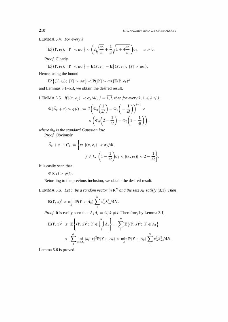
210 S. V. NAGAEV AND V. I. CHEBOTAREV
LEMMA 5.4. For everyk
E{(Y, ek); |Y | < aσ
}<
(2
√n0
n+ 1
a
√1+ 4
n0
n
)σk, a > 0.
Proof.Clearly
E{(Y, ek); |Y | < aσ
} = E(Y, ek)− E{(Y, ek); |Y | > aσ
}.
Hence, using the bound
E2{(Y, ek); |Y | > aσ} < P(|Y | > aσ
)E(Y, ek)2
and Lemmas 5.1–5.3, we obtain the desired result.
LEMMA 5.5. If |(x, ej )| < σj/4l, j = 1, l, then for everyk, 16 k 6 l,
8(Ak + x) > q(l) := 2(80
(1
4l
)−80
(− 1
4l
))l−1
×
×(80
(2− 1
4l
)−80
(1− 1
4l
)),
where80 is the standard Gaussian law.Proof.Obviously
Ak + x ⊃ Ck :={x: |(x, ej )| < σj/4l,
j 6= k,(
1− 1
4l
)σj < |(x, ek)| < 2− 1
4l
}.
It is easily seen that
8(Ck) > q(l).
Returning to the previous inclusion, we obtain the desired result.
LEMMA 5.6. LetY be a random vector inRN and the setsAk satisfy(3.1).Then
E(Y, x)2 > mink
P(Y ∈ Ak)N∑1
x2mλ
2m/4N.
Proof. It is easily seen thatAkAl = ∅, k 6= l. Therefore, by Lemma 3.1,
E(Y, x)2 > E
{(Y, x)2; Y ∈
N⋃1
Ak
}=
N∑1
E{(Y, x)2; Y ∈ Ak
}>
N∑1
infal∈Ak
(al, x)2P(Y ∈ Ak) > min
kP(Y ∈ Ak)
N∑1
x2mλ
2m/4N.
Lemma 5.6 is proved.
ON THE ACCURACY OF GAUSSIAN APPROXIMATION IN HILBERT SPACE 211
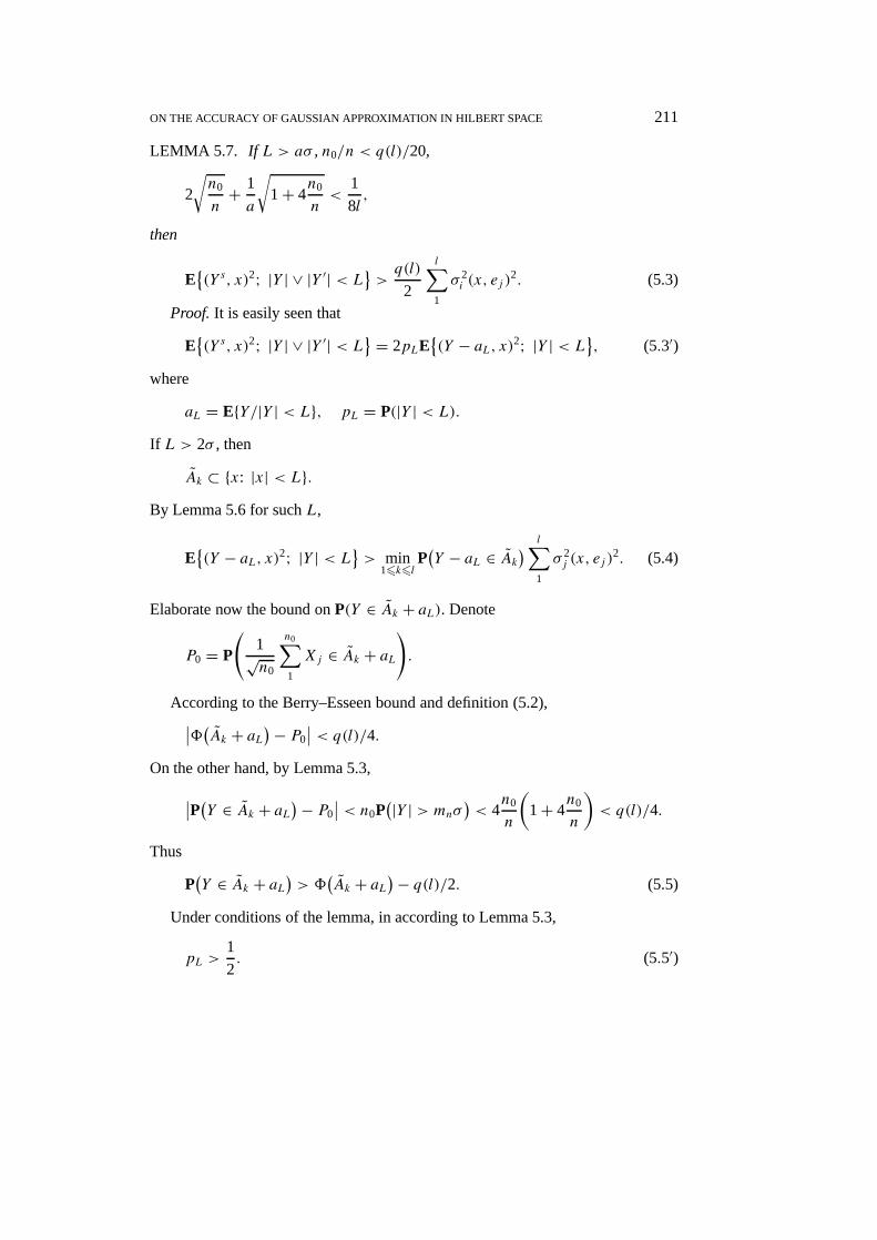
LEMMA 5.7. If L > aσ , n0/n < q(l)/20,
2
√n0
n+ 1
a
√1+ 4
n0
n<
1
8l,
then
E{(Y s, x)2; |Y | ∨ |Y ′| < L} > q(l)
2
l∑1
σ 2i (x, ej )
2. (5.3)
Proof. It is easily seen that
E{(Y s, x)2; |Y | ∨ |Y ′| < L} = 2pLE
{(Y − aL, x)2; |Y | < L
}, (5.3′)
where
aL = E{Y/|Y | < L}, pL = P(|Y | < L).If L > 2σ , then
Ak ⊂ {x: |x| < L}.By Lemma 5.6 for suchL,
E{(Y − aL, x)2; |Y | < L
}> min
16k6lP(Y − aL ∈ Ak
) l∑1
σ 2j (x, ej )
2. (5.4)
Elaborate now the bound onP(Y ∈ Ak + aL). Denote
P0 = P
(1√n0
n0∑1
Xj ∈ Ak + aL).
According to the Berry–Esseen bound and definition (5.2),∣∣8(Ak + aL)− P0
∣∣ < q(l)/4.On the other hand, by Lemma 5.3,∣∣P(Y ∈ Ak + aL)− P0
∣∣ < n0P(|Y | > mnσ
)< 4
n0
n
(1+ 4
n0
n
)< q(l)/4.
Thus
P(Y ∈ Ak + aL
)> 8
(Ak + aL
)− q(l)/2. (5.5)
Under conditions of the lemma, in according to Lemma 5.3,
pL >1
2. (5.5′)
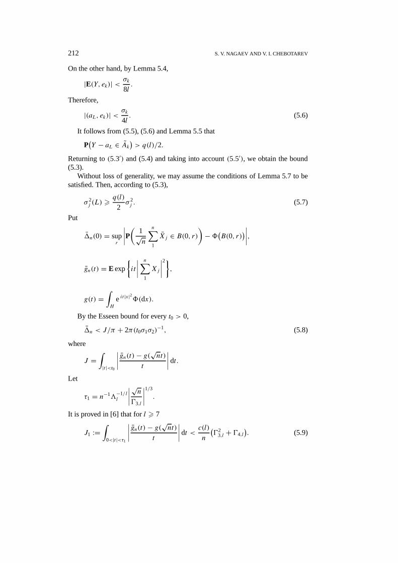
212 S. V. NAGAEV AND V. I. CHEBOTAREV
On the other hand, by Lemma 5.4,
|E(Y, ek)| < σk
8l.
Therefore,
|(aL, ek)| < σk
4l. (5.6)
It follows from (5.5), (5.6) and Lemma 5.5 that
P(Y − aL ∈ Ak
)> q(l)/2.
Returning to(5.3′) and (5.4) and taking into account(5.5′), we obtain the bound(5.3).
Without loss of generality, we may assume the conditions of Lemma 5.7 to besatisfied. Then, according to (5.3),
σ 2j (L) >
q(l)
2σ 2j . (5.7)
Put
1n(0) = supr
∣∣∣∣P( 1√n
n∑1
Xj ∈ B(0, r))−8(B(0, r))∣∣∣∣,
gn(t) = E exp
{it
∣∣∣∣ n∑1
Xj
∣∣∣∣2},g(t) =
∫H
eit |x|28(dx).
By the Esseen bound for everyt0 > 0,
1n < J/π + 2π(t0σ1σ2)−1, (5.8)
where
J =∫|t |<t0
∣∣∣∣ gn(t)− g(√nt)t
∣∣∣∣ dt.Let
τ1 = n−13−1/ ll
∣∣∣∣√n03,l
∣∣∣∣1/3.It is proved in [6] that forl > 7
J1 :=∫
0<|t |<τ1
∣∣∣∣ gn(t)− g(√nt)t
∣∣∣∣dt < c(l)
n
(02
3,l + 04,l). (5.9)
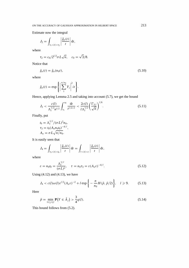
ON THE ACCURACY OF GAUSSIAN APPROXIMATION IN HILBERT SPACE 213
Estimate now the integral
J2 =∫τ1<|t |<τ2
∣∣∣∣ gn(t)t∣∣∣∣ dt,
where
τ2 = c0/2l/2σL
√n, c0 =
√3/8.
Notice that
gn(t) = gn(n0t), (5.10)
where
gn(t) = exp
{∣∣∣∣ n/n0∑1
Yj
∣∣∣∣2it}.
Hence, applying Lemma 2.5 and taking into account (5.7), we get the bound
J2 <c(l)
31/2l nl/2
∫ ∞τ1
dt
t l/2+1<
2c(l)
l31/2l
(03,l√n
)l/6. (5.11)
Finally, put
t0 = 31/ ll /(σL)2n0,
τ3 = t0(Ann0t0)−4/ l,
An = σL√n/n0.
It is easily seen that
J4 =∫τ3<|t |<t0
∣∣∣∣ gn(t)t∣∣∣∣dt = ∫
τ<|t |<ε
∣∣∣∣ gn(t)t∣∣∣∣dt,
where
ε = n0t0 = 31/ ll
(σL)2, τ = n0τ3 = ε(Anε)−4/ l. (5.12)
Using (4.12) and (4.13), we have
J4 < c(l)ω(l)εl/2(Anε)
−2+ l exp{− n
n0H(p, p/2)
}, l > 9. (5.13)
Here
p = min16j6l
P(Y ∈ Aj
)>
3
4q(l). (5.14)
This bound follows from (5.2).
214 S. V. NAGAEV AND V. I. CHEBOTAREV
We are to take into account that
inf16j6l
P(Y ∈ A±j
)>
3
4q(l)
as well.It is easy to check that
ω(l)εl/2(Anε)−2 = n0
n
(σL
31/ ll
)2
. (5.15)
It follows from (5.13)–(5.15) that
J4 < c(l)n0
n
(σL
31/ ll
)2
, l > 9. (5.16)
Using Lemma 2.4 and (5.10), we have
J3 :=∫τ26t<τ3
∣∣∣∣ gn(t)t∣∣∣∣ dt < ∫
|t |<τ
∣∣∣∣ gn(t)t∣∣∣∣ dt < c(l)(σL)l
31/2l
∫ τ
0t l/2−1 dt.
By (5.12) and (5.15)
(σL)l
31/ ll
τ l/2 = n0
n
(σL
31/ ll
)2
.
Consequently,
J3 < c(l)
(σL
31/ ll
)2n0
n. (5.17)
Notice that
J5 :=∫ t0
τ1
∣∣∣∣g(√nt)t
∣∣∣∣dt < c(l)(03,l√n
)l/6. (5.18)
It is clear that
J 65∑1
J5.
Hence, collecting the bounds (5.9), (5.11), (5.16)–(5.18), we get
J 6 c(l, l′)n
(02
3,l + 04,l + n0
(σL
31/ l′l′
)2
L2l′
), l > 13, l′ > 9. (5.19)
It follows from (5.8), (5.2) and (5.19) that
1n(0) <c(l, l′)n
(02
3,l + 04,l +(σL
31/ l′l′
)2
L2l′
), l > 13, l′ > 9.
ON THE ACCURACY OF GAUSSIAN APPROXIMATION IN HILBERT SPACE 215
Hence, puttingL = aσ and taking into account that
1n(0) < 1n(0)+ nβ4
σ 4m4n
,
we obtain the desired result.
References
1. Bentkus, V. and Götze, F.: Optimal rates of convergence in functional theorems for quadraticforms, Preprint 95–091, SFB343, Universität Bielefeld, 1995.
2. Bentkus, V. and Götze, F.: Optimal rates of convergence in CLT for quadratic forms,Ann.Probab.24 (1996), 406–490.
3. Bentkus, V. and Götze, F.: On lattice point problem for ellipsoids,Acta Arith. 80(2) (1997),101–125.
4. Bentkus, V. and Götze, F.: Uniform rates of convergence in the CLT for quadratic forms inmultidimensional spaces,Probab. Theory Related Fields109(1997), 367–416.
5. Nagaev, S. V.: On the rate of convergence to the normal law in a Hilbert space,Theory Probab.Appl.30 (1985), 19–37.
6. Nagaev, S. V. and Chebotarev, V. I.: A refinement of error estimate of the normal approximationin a Hilbert space,Siberian Math. J.27 (1986), 434–450.
7. Nagaev, S. V.: Concentration functions and approximation with infinitely divisible laws inHilbert space, Preprint, 90-094, SFB343, Universität Bielefeld, 1990.
![On Stein’s method for multivariate normal approximation · Chatterjee [3], where several abstract normal approximation theorems, for approx-imating by standard Gaussian random vectors,](https://img.pdfslide.us/doc/110x75/5f53a0f2897d984734626843/on-steinas-method-for-multivariate-normal-approximation-chatterjee-3-where.jpg)