Auton RobotDOI 10.1007/s10514-008-9095-6

Geodesic Gaussian kernels for value function approximation

Masashi Sugiyama · Hirotaka Hachiya ·Christopher Towell · Sethu Vijayakumar

Received: 6 July 2007 / Accepted: 6 June 2008© Springer Science+Business Media, LLC 2008

Abstract The least-squares policy iteration approach worksefficiently in value function approximation, given appropri-ate basis functions. Because of its smoothness, the Gaussiankernel is a popular and useful choice as a basis function.However, it does not allow for discontinuity which typicallyarises in real-world reinforcement learning tasks. In this pa-per, we propose a new basis function based on geodesicGaussian kernels, which exploits the non-linear manifoldstructure induced by the Markov decision processes. Theusefulness of the proposed method is successfully demon-strated in simulated robot arm control and Khepera robotnavigation.

The current paper is a complete version of our earlier manuscript(Sugiyama et al. 2007). The major differences are that we includedmore technical details of the proposed method in Sect. 3, discussionson the relation to related methods in Sect. 4, and the application tomap building in Sect. 6. A demo movie of the proposed methodapplied in simulated robot arm control and Khepera robot navigationis available from http://sugiyama-www.cs.titech.ac.jp/~sugi/2008/GGKvsOGK.wmv.

M. Sugiyama (�) · H. HachiyaDepartment of Computer Science, Tokyo Institute of Technology,2-12-1, O-okayama, Meguro-ku, Tokyo, 152-8552, Japane-mail: sugi@cs.titech.ac.jp

H. Hachiyae-mail: hachiya@sg.cs.titech.ac.jp

M. Sugiyama · C. Towell · S. VijayakumarSchool of Informatics, University of Edinburgh, The King’sBuildings, Mayfield Road, Edinburgh EH9 3JZ, UK

C. Towelle-mail: C.C.Towell@sms.ed.ac.uk

S. Vijayakumare-mail: sethu.vijayakumar@ed.ac.uk

Keywords Reinforcement learning · Value functionapproximation · Markov decision process · Least-squarespolicy iteration · Gaussian kernel

1 Introduction

Designing a flexible controller of a complex robot is a dif-ficult and time-consuming task for robot engineers. Rein-forcement learning (RL) is an approach that tries to easethis difficulty (Sutton and Barto 1998). Value function ap-proximation is an essential ingredient in RL, especially inthe context of solving Markov Decision Processes (MDPs)using policy iteration methods. Since real robots often in-volve large discrete state-spaces or continuous state-spaces,it becomes necessary to use function approximation meth-ods to represent the value functions. A least-squares ap-proach using a linear combination of predetermined under-complete basis functions has shown to be promising in thistask (Lagoudakis and Parr 2003; Osentoski and Mahadevan2007). For general function approximation, Fourier func-tions (trigonometric polynomials) Gaussian kernels (Girosiet al. 1995), and wavelets (Daubechies 1992) are typical ba-sis function choices and they have been employed in ro-botics domains (Lagoudakis and Parr 2003; Kolter and Ng2007). Normalized-Gaussian bases (Morimoto and Doya2007) as well as local linear approximation are also usedin humanoid robot control (Vijayakumar et al. 2002).

Fourier bases (global functions) and Gaussian kernels(localized functions) have certain smoothness propertiesthat make them particularly useful for modeling inherentlysmooth, continuous functions. Wavelets provide basis func-tions at various different scales and may also be employedfor approximating smooth functions with local discontinu-ity.

Auton Robot

Typical value functions in RL tasks are predominantlysmooth with some discontinuous parts (Mahadevan 2005).To illustrate this, let us consider a toy RL task of guiding anagent to a goal in a grid world (see Fig. 1a). In this task, astate corresponds to a two-dimensional Cartesian position ofthe agent. The agent cannot move over the wall, so the valuefunction of this task is highly discontinuous across the wall.On the other hand, the value function is smooth along themaze since neighboring reachable states in the maze havesimilar values (see Fig. 1b). Due to the discontinuity, sim-ply employing Fourier functions or Gaussian kernels as ba-sis functions tend to produce undesired, non-optimal resultsaround the discontinuity, affecting the overall performancesignificantly (see Fig. 3b). Wavelets could be a viable al-ternative, but are over-complete bases—one has to appro-priately choose a subset of basis functions, which is not astraightforward task in practice.

Recently, Mahadevan (2005) proposed considering valuefunctions defined not on the Euclidean space, but on graphsinduced by the MDPs (see Fig. 1c). Value functions whichusually contain discontinuity in the Euclidean domain (e.g.,across the wall) could be smooth on graphs (e.g., along themaze) if the graph is built appropriately. Hence, approximat-ing value functions on graphs can be expected to work betterthan approximating them in the Euclidean domain.

The spectral graph theory (Chung 1997) showed thatFourier-like smooth bases on graphs are given as minoreigenvectors of the graph-Laplacian matrix (see Fig. 2c).However, their global nature implies that the overall accu-racy of this method tends to be degraded by local noise.Coifman and Maggioni (2006) defined diffusion wavelets,which posses natural multi-resolution structure on graphs(see Fig. 2d). Mahadevan and Maggioni (2006) showed thatdiffusion wavelets could be employed in value function ap-proximation, although the issue of choosing a suitable sub-set of basis functions from the over-complete set is notdiscussed—determining the resolution level as well as thesmoothness within the level may not be straightforward inpractice.

In the machine learning community, Gaussian kernelsseem to be more popular than Fourier functions or waveletsbecause of their locality and smoothness (Girosi et al. 1995;Vapnik 1998; Schölkopf and Smola 2002). Furthermore,Gaussian kernels have ‘centers’, which alleviates the dif-ficulty of basis subset choice, e.g., uniform allocation(Lagoudakis and Parr 2003) or sample-dependent alloca-tion (Engel et al. 2005). In this paper, we therefore de-fine Gaussian kernels on graphs (which we call geodesicGaussian kernel), and propose using them for value func-tion approximation (see Fig. 2a). Our definition of Gaussiankernels on graphs employs the shortest paths between statesrather than the Euclidean distance, which can be computedefficiently using the Dijkstra algorithm (Dijkstra 1959;

Fredman and Tarjan 1987). Moreover, an effective use ofGaussian kernels opens up the possibility to exploit the re-cent advances in using Gaussian processes for temporal-difference learning (Engel et al. 2005).

Basis functions defined on the state space can be usedfor approximating the state-action value function by extend-ing them over the action space. This is typically done bysimply copying the basis functions over the action space(Lagoudakis and Parr 2003; Mahadevan 2005). In this pa-per, we propose a new strategy for this extension, whichtakes into account the transition after taking actions. Thisnew strategy is demonstrated to work very well when thetransition is predominantly deterministic.

The paper describes the notations employed for the RLproblem succinctly in Sect. 2. Section 3 formulates theGaussian kernel based basis functions on graphs, including amethod to generalize them to the continuous domains. Sec-tion 4 qualitatively discusses the characteristics of the pro-posed geodesic Gaussian kernel and the relation between theproposed and existing basis functions. Section 5 is devotedto extensive experimental comparison between the proposedand existing basis functions. Section 6 shows applications ofthe proposed method in simulated kinematic robot arm con-trol and mobile robot navigation. Section 7 provides con-cluding remarks and future directions.

2 Formulation of the reinforcement learning problem

In this section, we briefly introduce the notation and rein-forcement learning (RL) formulation that we will use acrossthe manuscript.

2.1 Markov decision processes

Let us consider a Markov decision process (MDP) specifiedby

(S,A,P,R,γ ), (1)

where

• S = {s(1), s(2), . . . , s(n)} is a finite1 set of states,• A = {a(1), a(2), . . . , a(m)} is a finite set of actions,• P(s′|s, a) : S ×A× S → [0,1] is the conditional proba-

bility of making a transition to state s′ if action a is takenin state s,

• R(s, a, s′) : S × A × S → R is an immediate reward formaking a transition from s to s′ by action a,

• γ ∈ [0,1) is the discount factor for future rewards.

1For the moment, we focus on discrete state spaces. In Sect. 3.4, weextend the proposed method to continuous state spaces.

Auton Robot

The expected reward R(s, a) for a state-action pair (s, a) isgiven as

R(s, a) =∑

s′∈SP(s′|s, a)R(s, a, s′). (2)

Let

π(s) : S →A (3)

be a deterministic policy which the agent follows. In thispaper, we focus on deterministic policies since there alwaysexists an optimal deterministic policy (Lagoudakis and Parr2003). Let

Qπ(s, a) : S ×A → R (4)

be a state-action value function for policy π , which indicatesthe expected long-term discounted sum of rewards the agentreceives when the agent takes action a in state s and followspolicy π thereafter. Qπ(s, a) satisfies the following Bellmanequation:

Qπ(s, a) = R(s, a) + γ∑

s′∈SP(s′|s, a)Qπ(s′,π(s′)). (5)

The goal of RL is to obtain a policy which produces themaximum amount of long-term rewards. The optimal policyπ∗(s) is defined as

π∗(s) = argmaxa∈A

Q∗(s, a), (6)

where Q∗(s, a) is the optimal state-action value function de-fined by

Q∗(s, a) = maxπ

Qπ(s, a). (7)

2.2 Least-squares policy iteration

In practice, the optimal policy π∗(s) cannot be directly ob-tained since R(s, a) and P(s′|s, a) are usually unknown;even when they are known, direct computation of π∗(s) isoften intractable.

To cope with this problem, Lagoudakis and Parr (2003)proposed approximating the state-action value functionQπ(s, a) using a linear model:

Qπ (s, a;w) =k∑

i=1

wiφi(s, a), (8)

where k is the number of basis functions which is usu-ally chosen to be much smaller than |S| × |A|. w =(w1,w2, . . . ,wk)

� are the parameters to be learned, � de-notes the transpose, and {φi(s, a)}ki=1 are pre-determinedbasis functions. Note that k and {φi(s, a)}ki=1 can depend on

policy π , but we do not show the explicit dependence for thesake of simplicity. Assume we have roll-out samples from asequence of actions:

{(si , ai, ri , s′i )}ti=1, (9)

where each tuple denotes the agent experiencing a transitionfrom si to s′

i on taking action ai with immediate reward ri .We suppose that we have an enough amount of samples toestimate the transition probability P(s′|s, a).

Under the Least-Squares Policy Iteration (LSPI) formula-tion (Lagoudakis and Parr 2003), the parameter w is learnedso that the Bellman equation (5) is optimally approximatedin the least-squares sense.2 Consequently, based on the ap-proximated state-action value function with learned parame-ter wπ , the policy is updated as

π(s) ←− argmaxa∈A

Qπ (s, a; wπ ). (10)

Approximating the state-action value function and updatingthe policy is iteratively carried out until some convergencecriterion is met.

3 Gaussian kernels on graphs

In the LSPI algorithm, the choice of basis functions{φi(s, a)}ki=1 is an open design issue. Traditionally, Gaussiankernels have been a popular choice (Lagoudakis and Parr2003; Engel et al. 2005), but they cannot approximate dis-continuous functions well. Recently, more sophisticatedmethods of constructing suitable basis functions have beenproposed, which effectively make use of the graph struc-ture induced by MDPs (Mahadevan 2005). In this section,we introduce a novel way of constructing basis functionsby incorporating the graph structure while the relation tothe existing graph-based methods is discussed in the nextsection.

3.1 MDP-induced graph

Let G be a graph induced by an MDP, where states S arenodes of the graph and the transitions with non-zero transi-tion probabilities from one node to another are edges. Theedges may have weights determined, e.g., based on the tran-sition probabilities or the distance between nodes. The graphstructure corresponding to an example grid-world shown inFig. 1a is illustrated in Fig. 1c. In practice, such graph struc-ture (including the connection weights) is estimated from

2There are two alternative approaches: Bellman residual minimizationand fixed point approximation. We take the latter approach followingthe suggestion in Lagoudakis and Parr (2003).

Auton Robot

Fig. 1 An illustrative example of an RL task of guiding an agent to a goal in the grid world

samples of a finite length. We assume that the graph G isconnected. Typically, the graph is sparse in RL tasks, i.e.,

� � n(n − 1)/2, (11)

where � is the number of edges and n is the number of nodes.

3.2 Ordinary Gaussian kernels

Ordinary Gaussian kernels (OGKs) on the Euclidean spaceare defined as

K(s, s′) = exp

(−ED(s, s′)2

2σ 2

), (12)

where ED(s, s′) are the Euclidean distance between states s

and s′; for example,

ED(s, s′) = ‖x − x′‖, (13)

when the Cartesian positions of s and s′ in the state space aregiven by x and x′, respectively. σ 2 is the variance parameterof the Gaussian kernel.

The above Gaussian function is defined on the state spaceS , where s′ is treated as a center of the kernel. In orderto employ the Gaussian kernel in the LSPI algorithm, itneeds to be extended over the state-action space S × A.This is usually carried out by simply ‘copying’ the Gaussianfunction over the action space (Lagoudakis and Parr 2003;Mahadevan 2005). More precisely: let the total number k

of basis functions be mp, where m is the number of possibleactions and p is the number of Gaussian centers. For the i-thaction a(i) (∈ A) (i = 1,2, . . . ,m) and for the j -th Gaussian

center c(j) (∈ S) (j = 1,2, . . . , p), the (i + (j −1)m)-th ba-sis function is defined as

φi+(j−1)m(s, a) = I (a = a(i))K(s, c(j)), (14)

where I (·) is the indicator function:

I (a = a(i)) ={

1 if a = a(i),

0 otherwise.(15)

3.3 Geodesic Gaussian kernels

On graphs, a natural definition of the distance would bethe shortest path. So we define Gaussian kernels on graphsbased on the shortest path:

K(s, s′) = exp

(−SP(s, s′)2

2σ 2

), (16)

where SP(s, s′) denotes the shortest path from state s to states′. The shortest path on a graph can be interpreted as a dis-crete approximation to the geodesic distance on a non-linearmanifold (Chung 1997). For this reason, we call (16) a geo-desic Gaussian kernel (GGK).

Shortest paths on graphs can be efficiently computed us-ing the Dijkstra algorithm (Dijkstra 1959). With its naiveimplementation, computational complexity for computingthe shortest paths from a single node to all other nodes isO(n2), where n is the number of nodes. If the Fibonacciheap is employed, computational complexity can be reducedto O(n logn + �) (Fredman and Tarjan 1987), where � isthe number of edges. Since the graph in value function ap-proximation problems is typically sparse (i.e., � � n2), us-ing the Fibonacci heap provides significant computational

Auton Robot

gains. Furthermore, there exist various approximation algo-rithms which are computationally very efficient (see Gold-berg and Harrelson 2005 and references therein).

Analogous to OGKs, we need to extend GGKs to thestate-action space for using them in the LSPI method.A naive way is to just employ (14), but this can cause a‘shift’ in the Gaussian centers since the state usually changeswhen some action is taken. To incorporate this transition,we propose defining the basis functions as the expectationof Gaussian functions after transition, i.e.,

φi+(j−1)m(s, a) = I (a = a(i))∑

s′∈SP(s′|s, a)K(s′, c(j)).

(17)

This shifting scheme is shown to work very well whenthe transition is predominantly deterministic (see Sects. 5and 6.1 for experimental evaluation).

3.4 Extension to continuous state spaces

So far, we focused on discrete state spaces. However, theconcept of GGKs can be naturally extended to continuousstate spaces, which is explained here. First, the continuousstate space is discretized, which gives a graph as a discreteapproximation to the non-linear manifold structure of thecontinuous state space. Based on the graph, we constructGGKs in the same way as the discrete case. Finally, the dis-crete GGKs are interpolated, e.g., using a linear method togive continuous GGKs.

Although this procedure discretizes the continuous statespace, it must be noted that the discretization is only forthe purpose of obtaining the graph as a discrete approxima-tion of the continuous non-linear manifold; the resulting ba-sis functions themselves are continuously interpolated andhence, the state space is still treated as continuous, as op-posed to other conventional discretization procedures.

4 Comparison to related basis function approaches

In this section, we discuss the characteristics of GGKs incomparison to existing basis functions using a toy RL task ofguiding an agent to a goal in a deterministic grid-world (seeFig. 1a). The agent can take 4 actions: up/down/left/right.Note that actions which make the agent collide with the wallare disallowed. A positive immediate reward of +1 is givenif the agent reaches a goal state; otherwise it receives noimmediate reward. The discount factor is set at γ = 0.9.

In this task, a state s corresponds to a two-dimensionalCartesian grid position x of the agent. For illustration pur-poses, let us display the state value function

V π(s) : S → R, (18)

which is the expected long-term discounted sum of rewardsthe agent receives when the agent takes actions followingpolicy π from state s. From the definition, it can be con-firmed that V π(s) is expressed in terms of Qπ(s, a) as

V π(s) = Qπ(s,π(s)). (19)

The optimal state value function V ∗(s) (in log-scale) is illus-trated in Fig. 1b. An MDP-induced graph structure estimatedfrom 20 series of random walk samples3 of length 500 is il-lustrated in Fig. 1c. Here, the edge weights in the graph areset at 1 (which is equivalent to the Euclidean distance be-tween two nodes).

4.1 Geodesic Gaussian kernels

An example of GGKs for this graph is depicted in Fig. 2a,where the variance of the kernel is set at a large value (σ 2 =30) for illustration purposes. The graph shows that GGKshave nice smooth surface along the maze, but not across thepartition between two rooms. Since GGKs have ‘centers’,they are extremely useful for adaptively choosing a subsetof bases, e.g., using a uniform allocation strategy, sample-dependent allocation strategy, or maze-dependent allocationstrategy of the centers—a practical advantage over somenon-ordered basis functions. Moreover, since GGKs are lo-cal by nature, the ill-effects of local noise is constrainedlocally—another property that is useful in practice.

The approximated value function obtained by 40 GGKs4

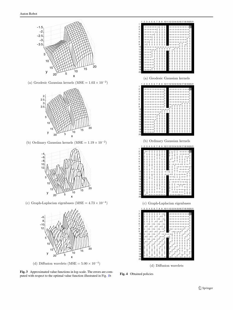
are depicted in Fig. 3a, where we put one GGK center atthe goal state and remaining 9 centers are chosen randomly.For GGKs, kernel functions are extended over the actionspace using the shifting scheme (see (17)) since the tran-sition is deterministic (see Sect. 3.3). The proposed GGK-based method produces a nice smooth function along themaze while the discontinuity around the partition betweentwo rooms is sharply maintained (cf. Fig. 1b). As a result,for this particular case, GGKs give the optimal policy (seeFig. 4a).

As discussed in Sect. 3.3, the sparsity of the state transi-tion matrix allows efficient and fast computations of short-est paths on the graph. Therefore, the LSPI algorithm withGGK-based bases is still computationally attractive (seeSect. 5). GGKs includes an open parameter, i.e., varianceσ 2 in (16). The effect of choice of the variance parameterwill be discussed in Sect. 5.

3More precisely, in each random walk, we choose an initial state ran-domly. Then, an action is chosen randomly and transition is made; thisis repeated 500 times. This entire procedure is independently repeated20 times to generate the training set.4Note that the total number k of basis functions is 160 since each GGKis copied over the action space as per (17).

Auton Robot

Fig. 2 Examples of basisfunctions

4.2 Ordinary Gaussian kernels

OGKs share some of the preferable properties of GGKs de-scribed above. However, as illustrated in Fig. 2b, the ‘tail’of OGKs extends beyond the partition between two rooms.Therefore, OGKs tend to undesirably ‘smooth’ out the dis-continuity of the value function around the barrier wall (see

Fig. 3b). This causes an error in the policy around the parti-tion (see x = 10, y = 2,3, . . . ,9 of Fig. 4b).

4.3 Graph-Laplacian eigenbases

Mahadevan (2005) proposed employing the smoothest vec-tors on graphs as bases in value function approximation.

Auton Robot

Fig. 3 Approximated value functions in log-scale. The errors are com-puted with respect to the optimal value function illustrated in Fig. 1b Fig. 4 Obtained policies

Auton Robot

According to the spectral graph theory (Chung 1997), suchsmooth bases are given by the minor eigenvectors of thegraph-Laplacian matrix, which are called graph-Laplacianeigenbases (GLEs). GLEs may be regarded as a natural ex-tension of Fourier bases to graphs.

Examples of GLEs are illustrated in Fig. 2c, showingthat they have a nice Fourier-like structure on the graph. Itshould be noted that GLEs are rather global in nature, im-plying that noise in a local region can potentially degradethe global quality of approximation. An advantage of GLEsis that they have a natural ordering of the basis functions ac-cording to the smoothness. This is practically very helpfulin choosing a subset of basis functions. Figure 3c depictsthe approximated value function in log-scale, where top 40smoothest GLEs out of 326 GLEs are used (note that the ac-tual number of bases is 160 because of the duplication overthe action space). It shows that GLEs globally give a verygood approximation (although the small local fluctuation issignificantly emphasized since the graph is in log-scale); in-deed, the mean squared error (MSE) between the approx-imated and optimal value functions described in the cap-tions of Fig. 3 shows that GLEs give a much smaller MSEthan GGKs and OGKs. However, the obtained value func-tion contains systematic local fluctuation and this results inan inappropriate policy (see Fig. 4c).

MDP-induced graphs are typically sparse. In such cases,the resultant graph-Laplacian matrix is also sparse andGLEs can be obtained just by solving a sparse eigenvalueproblem—which is computationally efficient (see Sect. 5).However, finding minor eigenvectors could be numericallyunstable.

4.4 Diffusion wavelets

Coifman and Maggioni (2006) proposed diffusion wavelets(DWs), which are a natural extension of wavelets to thegraph. The construction is based on a symmetrized randomwalk on a graph. It is diffused on the graph up to a desiredlevel, resulting in a multi-resolution structure. A detailed al-gorithm for constructing DWs and mathematical propertiesare described in Coifman and Maggioni (2006), so we omitthe detail here. We use the software provided by one of theauthors of the paper as it is.5

When constructing DWs, the maximum nest level ofwavelets and tolerance used in the construction algorithmneeds to be specified by users. We set the maximum nestlevel to 10 and the tolerance to 10−10, which are the defaultvalues used in the sample code. Examples of DWs are illus-trated in Fig. 2d, showing a nice multi-resolution structureon the graph. DWs are over-complete bases, so one has to

5http://www.math.yale.edu/~mmm82/DWCode_.html.

appropriately choose a subset of bases for better approxi-mation. Figure 3d depicts the approximated value functionobtained by DWs, where we chose the most global 40 DWsfrom 1626 over-complete DWs (note that the actual num-ber of bases is 160 because of the duplication over the ac-tion space). The choice of the subset bases could possiblybe enhanced using multiple heuristics; however, the currentchoice is reasonable since the Fig. 3d shows that DWs give amuch smaller MSE than Gaussian kernels. However, similarto GLEs, the obtained value function contains a lot of smallfluctuations (see Fig. 3d) and this results in an erroneouspolicy (see Fig. 4d).

Thanks to the multi-resolution structure, computation ofdiffusion wavelets can be carried out recursively. However,due to the over-completeness, it is still rather demanding incomputation time (see Sect. 5). Furthermore, appropriatelydetermining the tuning parameters as well as choosing anappropriate basis subset is not a straightforward task in prac-tice.

5 Experimental comparison

In this section, we report the results of extensive and sys-tematic experiments for illustrating the difference betweenGGKs and other basis function approaches.

We employ two deterministic grid-world problems illus-trated in Fig. 5, and evaluate the accuracy of approximatedvalue functions by computing the mean squared error (MSE)with respect to the optimal value function and the perfor-mance of obtained policies by calculating the fraction ofstates from which the agent can get to the goal optimally(i.e., in the shortest number of steps). 20 series of randomwalk of length 300 are gathered as training samples, whichare used for estimating the graph as well as the transitionprobability and expected reward. We set the edge weights inthe graph at 1 (which is equivalent to the Euclidean distancebetween two nodes).

This simulation is repeated 100 times for each maze andeach method, randomly changing training samples in eachrun. The mean of the above scores as a function of the num-ber of kernels is plotted in Figs. 6–9. Note that the actualnumber of bases is four times more because of the extensionof basis functions over the action space (see (14) and (17)).

First, we compare the performance of two kernel alloca-tion strategies in GGKs:

(i) Kernels are put at all the goal states and the remain-ing kernels are distributed uniformly over the maze; the‘shift’ strategy introduced in Sect. 3.3 is used.

(ii) All kernels are just uniformly distributed over the mazeand the ‘shift’ strategy is not used.

Auton Robot

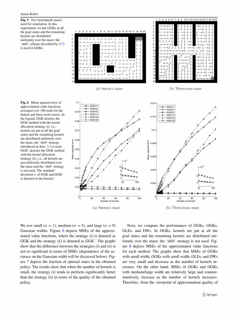
Fig. 5 Two benchmark mazesused for simulation. In thisexperiment, we put GGKs at allthe goal states and the remainingkernels are distributeduniformly over the maze; the‘shift’ scheme described by (17)is used in GGKs

Fig. 6 Mean squared error ofapproximated value functionsaveraged over 100 trials for theSutton and three room mazes. Inthe legend, GGK denotes theGGK method with the kernelallocation strategy (i), i.e.,kernels are put at all the goalstates and the remaining kernelsare distributed uniformly overthe maze; the ‘shift’ strategyintroduced in Sect. 3.3 is used.GGK’ denotes the GGK methodwith the kernel allocationstrategy (ii), i.e., all kernels arejust uniformly distributed overthe maze and the ‘shift’ strategyis not used. The standarddeviation σ of GGK and GGK’is denoted in the bracket

We test small (σ = 1), medium (σ = 5), and large (σ = 9)Gaussian widths. Figure 6 depicts MSEs of the approxi-mated value functions, where the strategy (i) is denoted asGGK and the strategy (ii) is denoted as GGK’. The graphsshow that the difference between the strategies (i) and (ii) isnot so significant in terms of MSEs (dependence of the ac-curacy on the Gaussian width will be discussed below). Fig-ure 7 depicts the fraction of optimal states in the obtainedpolicy. The results show that when the number of kernels issmall, the strategy (i) tends to perform significantly betterthan the strategy (ii) in terms of the quality of the obtainedpolicy.

Next, we compare the performance of GGKs, OGKs,GLEs, and DWs. In OGKs, kernels are put at all thegoal states and the remaining kernels are distributed uni-formly over the maze; the ‘shift’ strategy is not used. Fig-ure 8 depicts MSEs of the approximated value functionsfor each method. The graphs show that MSEs of GGKswith small width, OGKs with small width, GLEs, and DWsare very small and decrease as the number of kernels in-creases. On the other hand, MSEs of GGKs and OGKswith medium/large width are relatively large and counter-intuitively, increase as the number of kernels increases.Therefore, from the viewpoint of approximation quality of

Auton Robot

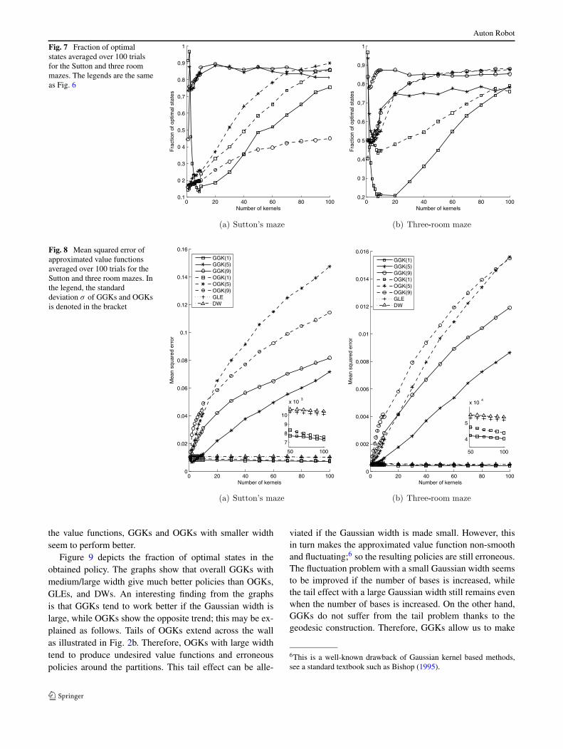
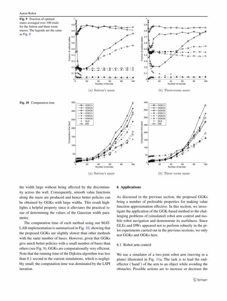
Fig. 7 Fraction of optimalstates averaged over 100 trialsfor the Sutton and three roommazes. The legends are the sameas Fig. 6

Fig. 8 Mean squared error ofapproximated value functionsaveraged over 100 trials for theSutton and three room mazes. Inthe legend, the standarddeviation σ of GGKs and OGKsis denoted in the bracket

the value functions, GGKs and OGKs with smaller widthseem to perform better.

Figure 9 depicts the fraction of optimal states in theobtained policy. The graphs show that overall GGKs withmedium/large width give much better policies than OGKs,GLEs, and DWs. An interesting finding from the graphsis that GGKs tend to work better if the Gaussian width islarge, while OGKs show the opposite trend; this may be ex-plained as follows. Tails of OGKs extend across the wallas illustrated in Fig. 2b. Therefore, OGKs with large widthtend to produce undesired value functions and erroneouspolicies around the partitions. This tail effect can be alle-

viated if the Gaussian width is made small. However, thisin turn makes the approximated value function non-smoothand fluctuating;6 so the resulting policies are still erroneous.The fluctuation problem with a small Gaussian width seemsto be improved if the number of bases is increased, whilethe tail effect with a large Gaussian width still remains evenwhen the number of bases is increased. On the other hand,GGKs do not suffer from the tail problem thanks to thegeodesic construction. Therefore, GGKs allow us to make

6This is a well-known drawback of Gaussian kernel based methods,see a standard textbook such as Bishop (1995).

Auton Robot

Fig. 9 Fraction of optimalstates averaged over 100 trialsfor the Sutton and three roommazes. The legends are the sameas Fig. 8

Fig. 10 Computation time

the width large without being affected by the discontinu-ity across the wall. Consequently, smooth value functionsalong the maze are produced and hence better policies canbe obtained by GGKs with large widths. This result high-lights a helpful property since it alleviates the practical is-sue of determining the values of the Gaussian width para-meter.

The computation time of each method using our MAT-LAB implementation is summarized in Fig. 10, showing thatthe proposed GGKs are slightly slower than other methodswith the same number of bases. However, given that GGKsgive much better policies with a small number of bases thanothers (see Fig. 9), GGKs are computationally very efficient.Note that the running time of the Dijkstra algorithm was lessthan 0.1 second in the current simulations, which is negligi-bly small; the computation time was dominated by the LSPIiteration.

6 Applications

As discussed in the previous section, the proposed GGKsbring a number of preferable properties for making valuefunction approximation effective. In this section, we inves-tigate the application of the GGK-based method to the chal-lenging problems of (simulated) robot arm control and mo-bile robot navigation and demonstrate its usefulness. SinceGLEs and DWs appeared not to perform robustly in the pi-lot experiments carried out in the previous sections, we onlytest GGKs and OGKs here.

6.1 Robot arm control

We use a simulator of a two-joint robot arm (moving in aplane) illustrated in Fig. 11a. The task is to lead the end-effector (‘hand’) of the arm to an object while avoiding theobstacles. Possible actions are to increase or decrease the

Auton Robot

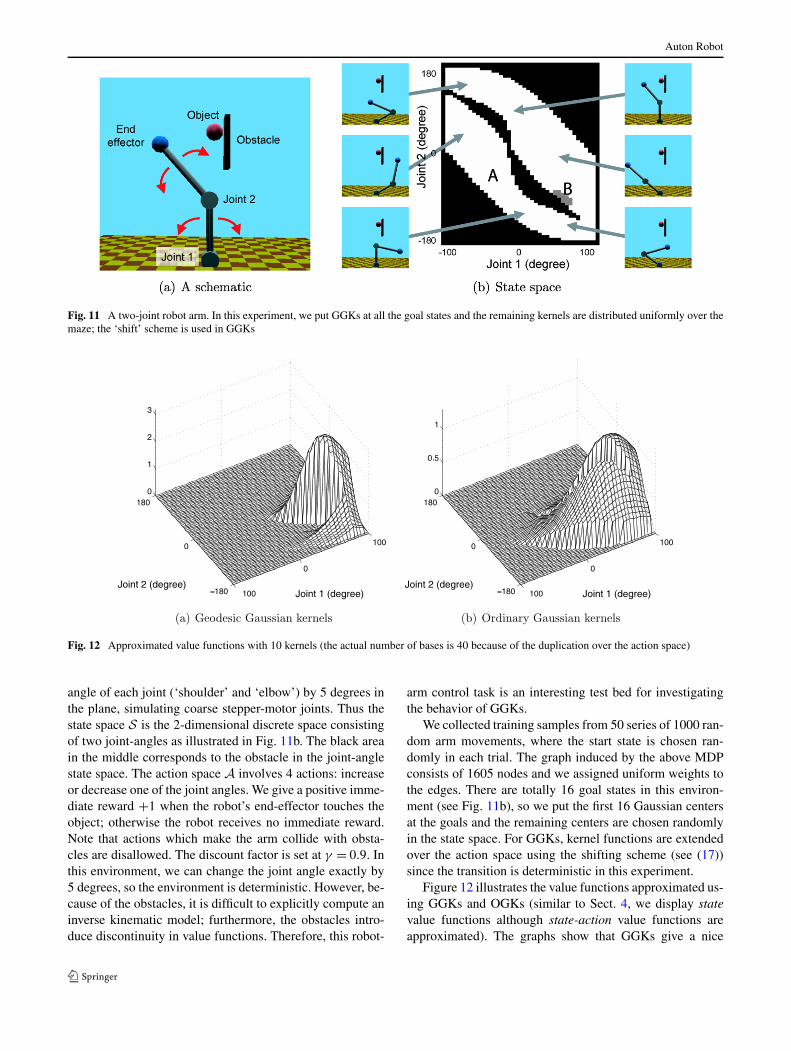
Fig. 11 A two-joint robot arm. In this experiment, we put GGKs at all the goal states and the remaining kernels are distributed uniformly over themaze; the ‘shift’ scheme is used in GGKs

Fig. 12 Approximated value functions with 10 kernels (the actual number of bases is 40 because of the duplication over the action space)

angle of each joint (‘shoulder’ and ‘elbow’) by 5 degrees inthe plane, simulating coarse stepper-motor joints. Thus thestate space S is the 2-dimensional discrete space consistingof two joint-angles as illustrated in Fig. 11b. The black areain the middle corresponds to the obstacle in the joint-anglestate space. The action space A involves 4 actions: increaseor decrease one of the joint angles. We give a positive imme-diate reward +1 when the robot’s end-effector touches theobject; otherwise the robot receives no immediate reward.Note that actions which make the arm collide with obsta-cles are disallowed. The discount factor is set at γ = 0.9. Inthis environment, we can change the joint angle exactly by5 degrees, so the environment is deterministic. However, be-cause of the obstacles, it is difficult to explicitly compute aninverse kinematic model; furthermore, the obstacles intro-duce discontinuity in value functions. Therefore, this robot-

arm control task is an interesting test bed for investigatingthe behavior of GGKs.

We collected training samples from 50 series of 1000 ran-dom arm movements, where the start state is chosen ran-domly in each trial. The graph induced by the above MDPconsists of 1605 nodes and we assigned uniform weights tothe edges. There are totally 16 goal states in this environ-ment (see Fig. 11b), so we put the first 16 Gaussian centersat the goals and the remaining centers are chosen randomlyin the state space. For GGKs, kernel functions are extendedover the action space using the shifting scheme (see (17))since the transition is deterministic in this experiment.

Figure 12 illustrates the value functions approximated us-ing GGKs and OGKs (similar to Sect. 4, we display statevalue functions although state-action value functions areapproximated). The graphs show that GGKs give a nice

Auton Robot

Fig. 13 Number of successful trials

smooth surface with obstacle-induced discontinuity sharplypreserved, while OGKs tend to smooth out the discontinuity.This makes a significant difference in avoiding the obstacle:from ‘A’ to ‘B’ in Fig. 11b, the GGK-based value functionresults in a trajectory that avoids the obstacle (see Fig. 12a).On the other hand, the OGK-based value function yields atrajectory that tries to move the arm through the obstacle byfollowing the gradient upward (see Fig. 12b), causing thearm to get stuck behind the obstacle.7

Figure 13 summarizes the performance of GGKs andOGKs measured by the percentage of successful trials (i.e.,the end-effector reaches the object) averaged over 30 in-dependent runs. More precisely, in each run, totally 50000training samples are collected using a different random seed,a policy is then computed by the GGK- or OGK-based LSPImethod, and the obtained policy is tested. This graph showsthat GGKs remarkably outperform OGKs since the arm cansuccessfully avoid the obstacle. The performance of OGKsdoes not go beyond 0.6 even when the number of kernels isincreased. This is caused by the ‘tail effect’ of OGKs; theOGK-based policy cannot lead the end-effector to the objectif it starts from the bottom-left half of the state space

When the number of kernels is increased, the perfor-mance of both GGKs and OGKs once gets worse at aroundk = 20. This would be caused by our kernel allocation strat-egy: the first 16 kernels are put at the goal states and the re-maining kernel centers are chosen randomly. When k is lessthan or equal to 16, the approximated value function tends tohave a unimodal profile since all kernels are put at the goalstates. However, when k is larger than 16, this unimodalityis broken and the surface of the approximated value func-tion has slight fluctuations, causing an error in policies and

7A demo movie is available from http://sugiyama-www.cs.titech.ac.jp/~sugi/2008/GGKvsOGK.wmv.

degrading performance at around k = 20. This performancedegradation tends to recover as the number of kernels is fur-ther increased.

Overall, the above result shows that when GGKs arecombined with our kernel-center allocation strategy, almostperfect policies can be obtained with a very small number ofkernels. Therefore, the proposed method is computationallyvery advantageous.

6.2 Robot agent navigation

The above simple robot-arm control simulation shows thatthe GGK method is promising. Here we apply GGKs to amore challenging task of mobile robot navigation, which in-volves a high-dimensional, very large state space.

We employ a Khepera robot illustrated in Fig. 14a on thenavigation task. A Khepera is equipped with 8 infra-red sen-sors (‘s1’ to ‘s8’ in the figure), each of which gives a mea-sure of the distance from the surrounding obstacles. Eachsensor produces a scalar value between 0 and 1023: the sen-sor obtains the maximum value 1023 if an obstacle is justin front of the sensor and the value decreases as the obsta-cle gets farther till it reaches the minimum value 0. There-fore, the state space S is 8-dimensional. The Khepera hastwo wheels and takes the following 4 defined actions: for-ward, left-rotation, right-rotation, and backward (i.e., the ac-tion space A contains 4 actions). The speed of the left andright wheels for each action is described in Fig. 14a in thebracket (the unit is pulse per 10 milliseconds). Note that thesensor values and the wheel speed are highly stochastic dueto the cross talk, sensor noise, slip etc. Furthermore, percep-tual aliasing occurs due to the limited range and resolutionof sensors. Therefore, the state transition is also highly sto-chastic. We set the discount factor at γ = 0.9.

The goal of the navigation task is to make the Kheperaexplore the environment as much as possible. To this end, wegive a positive reward +1 when the Khepera moves forwardand a negative reward −2 when the Khepera collides withan obstacle. We do not give any reward to the left/right ro-tation and backward actions. This reward design encouragesthe Khepera to go forward without hitting obstacles, throughwhich extensive exploration in the environment could beachieved.

We collected training samples from 200 series of 100 ran-dom movements in a fixed environment with several obsta-cles (see Fig. 15a). Then we constructed a graph from thegathered samples by discretizing the continuous state spaceusing the Self-Organizing Map (SOM) (Kohonen 1995).A SOM consists of neurons located on a regular grid. Eachneuron corresponds to a cluster and neurons are connected toadjacent ones by neighborhood relation. The SOM is similarto the k-means clustering algorithm, but it is different in thattopological structure of the entire map is taken into account;

Auton Robot

Fig. 14 Khepera robot. In this experiment, GGKs are distributed uniformly over the maze without the ‘shift’ scheme

Fig. 15 Simulationenvironment

by that, the entire space tends to be covered. The number ofnodes (states) in the graph is set at 696 (equivalent with theSOM map size of 24 × 29); this value is computed by thestandard rule-of-thumb formula 5

√n (Vesanto et al. 2000),

where n is the number of samples. The connectivity of thegraph is determined by state transitions occurred in the sam-ples, i.e., if there is a state transition from one node to an-other in the samples, an edge is established between thesetwo nodes and the edge weight is set according to the Euclid-ean distance between them.

Figure 14b illustrates an example of the obtained graphstructure. For visualization purposes, we projected the 8-dimensional state space onto a 2-dimensional subspace8

spanned by

(−1 −1 0 0 1 1 0 0),

(0 0 1 1 0 0 −1 −1).(20)

8We note that the projection is done only for the purpose of visualiza-tion; all the computations are carried out using the entire 8-dimensionaldata.

The i-th element in the above bases corresponds to the out-put of the i-th sensor (see Fig. 14a). The projection ontothis subspace roughly means that the horizontal axis corre-sponds to the distance to the left/right obstacle, while thevertical axis corresponds to the distance to the front/backobstacle. For clear visibility, we only displayed the edgeswhose weight is less than 250. Representative local poses ofthe Khepera with respect to the obstacles are illustrated forsalient nodes of the state-space MDP graph in Fig. 14b. Thisgraph has a notable feature: the nodes around the region ‘B’in the figure are directly connected to the nodes at ‘A’, butare very sparsely connected to the nodes at ‘C’, ‘D’, and ‘E’.This implies that the geodesic distance from ‘B’ to ‘C’, ‘B’to ‘D’, or ‘B’ to ‘E’ is typically larger than the Euclideandistance.

Since the transition from one state to another is highlystochastic in the current experiment, we decided to simplyduplicate the GGK function over the action space (see (14)).For obtaining continuous GGKs, GGK functions need to beinterpolated (see Sect. 3.4). We may employ a simple lin-ear interpolation method in general. However, the currentexperiment has unique characteristics—at least one of the

Auton Robot

Fig. 16 Examples of obtained policies. The symbols ‘↑’, ’↓’, ‘⊂’, and ‘⊃’ indicate forward, backward, left-rotation, and right-rotation actions

sensor values is always zero since the Khepera is never com-pletely surrounded by obstacles. Therefore, samples are al-ways on the surface of the 8-dimensional hypercube-shapedstate space. On the other hand, the node centers determinedby the SOM are not generally on the surface. This means thatany sample is not included in the convex hull of its nearestnodes and we need to extrapolate the function value. Here,we simply add the Euclidean distance between the sampleand its nearest node when computing kernel values; moreprecisely, for a state s that is not generally located on a nodecenter, the GGK-based basis function is defined as

φi+(j−1)m(s, a)

= I (a = a(i)) exp

(− (ED(s, s) + SP(s, c(j)))2

2σ 2

), (21)

where s is the node closest to s in the Euclidean distance.Figure 16 illustrates an example of actions selected at

each node by the GGK-based and OGK-based policies. Weused 100 kernels and set the width at 1000. The symbols‘↑’, ’↓’, ‘⊂’, and ‘⊃’ in the figure indicate forward, back-ward, left-rotation, and right-rotation actions. This showsthat there is a clear difference in the obtained policies at thestate ‘C’; the backward action is most likely to be taken bythe OGK-based policy while the left/right rotation are mostlikely to be taken by the GGK-based policy. This causes asignificant difference in the performance. To explain this,let us assume that the Khepera is at the state ‘C’, i.e., it facesa wall. The GGK-based policy guides the Khepera from ‘C’to ‘A’ via ‘D’ or ‘E’ by taking left/right rotation actions andit can avoid the obstacle successfully. On the other hand, theOGK-based policy tries to plan a path from ‘C’ to ‘A’ via ‘B’by activating the backward action; then, the forward action

Fig. 17 Average amount of exploration

is taken at ‘B’. Thus, the Khepera returns to ‘C’ again andends up moving back and forth between ‘C’ and ‘B’.9

For the performance evaluation, we use a more compli-cated environment than the one used for gathering trainingsamples (see Fig. 15). Thus we are evaluating how well theobtained policies can be generalized to an unknown envi-ronment. In this test environment, we let the Khepera runfrom a fixed starting position (see Fig. 15b) and take 150steps following the obtained policy. We compute the sumof rewards, i.e., +1 for the forward action. If the Khep-era collides with an obstacle before 150 steps, we stop theevaluation. The mean test performance over 30 independent

9A demo movie is available from http://sugiyama-www.cs.titech.ac.jp/~sugi/2008/GGKvsOGK.wmv.

Auton Robot

runs is depicted in Fig. 17 as a function of the number ofkernels. More precisely, in each run, we construct a graphbased on the training samples taken from the training envi-ronment and put the specified number of kernels randomlyon the graph. Then, a policy is learned by the GGK or OGK-based LSPI method using the training samples. Note that theactual number of bases is four times more because of theextension of basis functions over the action space. The testperformance is measured 5 times for each policy and the av-erage is outputted. Figure 17 shows that GGKs significantlyoutperform OGKs, demonstrating that GGKs are promisingeven in the challenging setting with a high-dimensional hugestate space.

Figure 18 depicts the computation time of each methodas a function of the number of kernels. This shows that thecomputation time monotonically increases as the numberof kernels increases and the GGK-based and OGK-basedmethods have comparable computation time. Given that the

Fig. 18 Computation time

GGK-based method works much better than the OGK-basedmethod with a smaller number of kernels (see Fig. 17), theproposed method could be regarded as a computationally ef-ficient alternative to the standard OGK-based method.

Finally, we apply the learned Khepera robot to map build-ing. Starting from an initial position (indicated by a squarein Fig. 19), the Khepera robot takes an action 2000 times fol-lowing the learned policy. We used 80 kernels with Gaussianwidth σ = 1000 in value function approximation. The re-sults of GGKs and OGKs are depicted in Fig. 19a and b.The graphs show that the GGK result gives a broader pro-file of the environment, while the OGK result only reveals alocal area around the initial position.

7 Conclusions and outlook

We proposed a new basis-construction method for valuefunction approximation. The proposed geodesic Gaussiankernels (GGKs) have several preferable properties such asthe smoothness along the graph and easy computability.We demonstrated the practical usefulness of the proposedmethod for challenging applications: both the robot-armreaching experiments with obstacles and the Khepera ex-ploration experiments showed quantitative improvements aswell as intuitive, interpretable behavioral advantages evidentfrom the experiments.

Experiments in Sect. 5 showed that GGKs with largewidth has larger MSEs than that with smaller width, butGGKs with large width gave better policies than that withsmaller width. We conjecture that GGKs with large widthgive smoother value functions and hence, result in stablepolicies. Although this explanation would be intuitively rea-sonable, it needs to be elucidated in a more rigorous way.

Fig. 19 Results of map building (cf. Fig. 15b)

Auton Robot

It is shown that the policies obtained by GGKs are notso sensitive to the choice of the width of the Gaussian ker-nels, i.e., a reasonably large width works very well. Thisis a very useful property in practice. Also, the heuristicsof putting Gaussian centers on goal states is shown towork quite well. Even so, it is an important future direc-tion to develop a method for optimally tuning the width aswell as the location parameters, e.g., based on the statisti-cal machine learning theory (Vapnik 1998; Hachiya et al.2008).

When the transition is highly stochastic (i.e., the transi-tion probability has a wide support), the graph constructedbased on the transition samples could be noisy. When an er-roneous transition results in a short-cut over obstacles, thegraph-based approach may not work well since the topol-ogy of the state space changes significantly. Therefore, it isan important future work to evaluate the robustness of theproposed approach under very noisy environment and to de-velop a more robust method of building a graph from noisytransition samples.

In Sect. 3.4, we extended the proposed GGKs to contin-uous state space. A significant research direction will be tofurther explore the properties of the continuous GGKs andtheir application to real world, high-dimensional problemssuch as planning in anthropomorphic robots.

We defined the Gaussian kernels on the state space, andthen extended them over the action space. If we define ba-sis functions directly on the state-action space, the qualityof value function approximation and the computational effi-ciency could be further improved. Our future research willfocus on this topic.

In this paper, we have focused on a batch RL scenariowhere samples are gathered in the beginning. Another prac-tical situation would be an online scenario where sam-ples are gathered incrementally through the policy iterationprocess. Such an online scenario induces an off-policy situ-ation, i.e., the policy used for data sampling and the policyused for evaluation are mismatched (Sutton and Barto 1998).It is therefore essential to develop a method that can handlethe off-policy situation efficiently, e.g., following the linesof Precup et al. (2000) and Hachiya et al. (2008).

Acknowledgements The authors acknowledge financial supportfrom MEXT (Grant-in-Aid for Young Scientists 17700142 and Grant-in-Aid for Scientific Research (B) 18300057), the Okawa Foundation,and EU Erasmus Mundus Scholarship.

References

Bishop, C. M. (1995). Neural networks for pattern recognition. Ox-ford: Clarendon.

Chung, F. R. K. (1997). Spectral graph theory. Providence: Am. Math.Soc.

Coifman, R., & Maggioni, M. (2006). Diffusion wavelets. Applied andComputational Harmonic Analysis, 21, 53–94.

Daubechies, I. (1992). Ten lectures on wavelets. Philadelphia: SIAM.

Dijkstra, E. W. (1959). A note on two problems in connexion withgraphs. Numerische Mathematik, 1, 269–271.

Engel, Y., Mannor, S., & Meir, R. (2005). Reinforcement learning withGaussian processes. In Proceedings of international conferenceon machine learning, Bonn, Germany.

Fredman, M. L., & Tarjan, R. E. (1987). Fibonacci heaps and theiruses in improved network optimization algorithms. Journal of theACM, 34, 569–615.

Girosi, F., Jones, M., & Poggio, T. (1995). Regularization theory andneural networks architectures. Neural Computation, 7, 219–269.

Goldberg, A. V., & Harrelson, C. (2005). Computing the shortest path:A* search meets graph theory. In 16th annual ACM-SIAM sympo-sium on discrete algorithms, Vancouver, Canada (pp. 156–165).

Hachiya, H., Akiyama, T., Sugiyama, M., & Peters, J. (2008). Adap-tive importance sampling with automatic model selection in valuefunction approximation. In Proceedings of the twenty-third AAAIconference on artificial intelligence (AAAI-08), Chicago, USA(pp. 1351–1356).

Kohonen, T. (1995). Self-organizing maps. Berlin: Springer.

Kolter, J. Z., & Ng, A. Y. (2007). Learning omnidirectional path fol-lowing using dimensionality reduction. In Proceedings of robot-ics: science and systems.

Lagoudakis, M. G., & Parr, R. (2003). Least-squares policy iteration.Journal of Machine Learning Research, 4, 1107–1149.

Mahadevan, S. (2005). Proto-value functions: Developmental rein-forcement learning. In Proceedings of international conferenceon machine learning, Bonn, Germany.

Mahadevan, S., & Maggioni, M. (2006). Value function approxima-tion with diffusion wavelets and Laplacian eigenfunctions. InAdvances in neural information processing systems (Vol. 18,pp. 843–850). Cambridge: MIT Press.

Morimoto, J., & Doya, K. (2007). Acquisition of stand-up behavior bya real robot using hierarchical reinforcement learning. Roboticsand Autonomous Systems, 36, 37–51.

Osentoski, S., & Mahadevan, S. (2007). Learning state-action basisfunctions for hierarchical MDPs. In Proceedings of the 24th in-ternational conference on machine learning.

Precup, D., Sutton, R. S., & Singh, S. (2000). Eligibility traces foroff-policy policy evaluation. In Proceedings of the seventeenth in-ternational conference on machine learning (pp. 759–766). SanMateo: Morgan Kaufmann.

Schölkopf, B., & Smola, A. J. (2002). Learning with kernels. Cam-bridge: MIT Press.

Sugiyama, M., Hachiya, H., Towell, C., & Vijayakumar, S. (2007).Value function approximation on non-linear manifolds for robotmotor control. In Proceedings of 2007 IEEE international confer-ence on robotics and automation (ICRA2007) (pp. 1733–1740).

Sutton, R. S., & Barto, G. A. (1998). Reinforcement learning: An in-troduction. Cambridge: MIT Press.

Vapnik, V. N. (1998). Statistical learning theory. New York: Wiley.

Vesanto, J., Himberg, J., Alhoniemi, E., & Parhankangas, J. (2000).SOM toolbox for Matlab 5 (Technical Report A57). Helsinki Uni-versity of Technology.

Vijayakumar, S., D’Souza, A., Shibata, T., Conradt, J., & Schaal, S.(2002). Statistical learning for humanoid robots. Autonomous Ro-bot, 12, 55–69.

Auton Robot

Masashi Sugiyama is an AssociateProfessor with the Department ofComputer Science at the Tokyo In-stitute of Technology, Japan. He re-ceived a Ph.D. in Computer Sciencefrom the Tokyo Institute of Technol-ogy in 2001. His research interestsinclude theories of machine learn-ing and their applications in roboticsand signal/image processing.

Hirotaka Hachiya received the B.E.degree from Soka University in2000 and the M.Sc. degree in infor-matics from the University of Edin-burgh in 2006. During 2000–2004,he worked in the web, softwareand robotic fields. He is currentlya Ph.D. candidate at the Tokyo In-stitute of Technology. His researchinterests are machine learning, rein-forcement learning and their appli-cation on robots.

Christopher Towell has an M.A.in Maths/Computer Science fromCambridge University, an MSc inInformatics from Edinburgh Univer-sity, and is currently studying fora Ph.D. in Neuroinformatics at Ed-inburgh University. He has severalyears experience as a commercialsoftware engineer. His research in-terests include statistical machinelearning, intelligent robotics andcomputational neuroscience.

Sethu Vijayakumar is a Reader(Associate Professor) with theSchool of Informatics at the Uni-versity of Edinburgh and the Direc-tor of the Institute for Perception,Action and Behavior (IPAB). Since2007, he holds a Senior ResearchFellowship of the Royal Academyof Engineering. He also holds addi-tional appointments as an AdjunctFaculty of the University of South-ern California, Los Angeles, a Re-search Scientist of the ATR Compu-tational Neuroscience Labs, Kyoto-Japan and a Visiting Research Sci-

entist at the RIKEN Brain Science Institute, Tokyo. He has a Ph.D.(’98) in Computer Science and Engineering from the Tokyo Instituteof Technology. Prof. Vijayakumar held the positions of Research As-sistant Professor (’01–’03) at USC and a Staff Scientist (’98–’00) atthe RIKEN Brain Science Institute before this appointment. His re-search interest spans a broad interdisciplinary curriculum involving ba-sic research in the fields of statistical machine learning, motor control,planning and optimization in autonomous systems and computationalneuroscience.