Extended Gaussian Images

Berthold K. P. Horn

Outline

Discrete Case: Convex Polyhedra Continuous Case: Smoothly Curved Objects Discrete Approximation: Needle Maps Tessellation of the Gaussian sphere:

Orientation Histograms Solids of Revolution

Outline

Discrete Case: Convex Polyhedra Continuous Case: Smoothly Curved Objects Discrete Approximation: Needle Maps Tessellation of the Gaussian sphere:

Orientation Histograms Solids of Revolution

Gaussian Image

What is a Gaussian Image?

Gaussian Image

What is a Gaussian Image?

A mapping of surface normals of an object onto the unit sphere (Gaussian sphere.) Tail lies at the center of the

Gaussian sphere Head lies on the surface of

the Gaussian sphere.

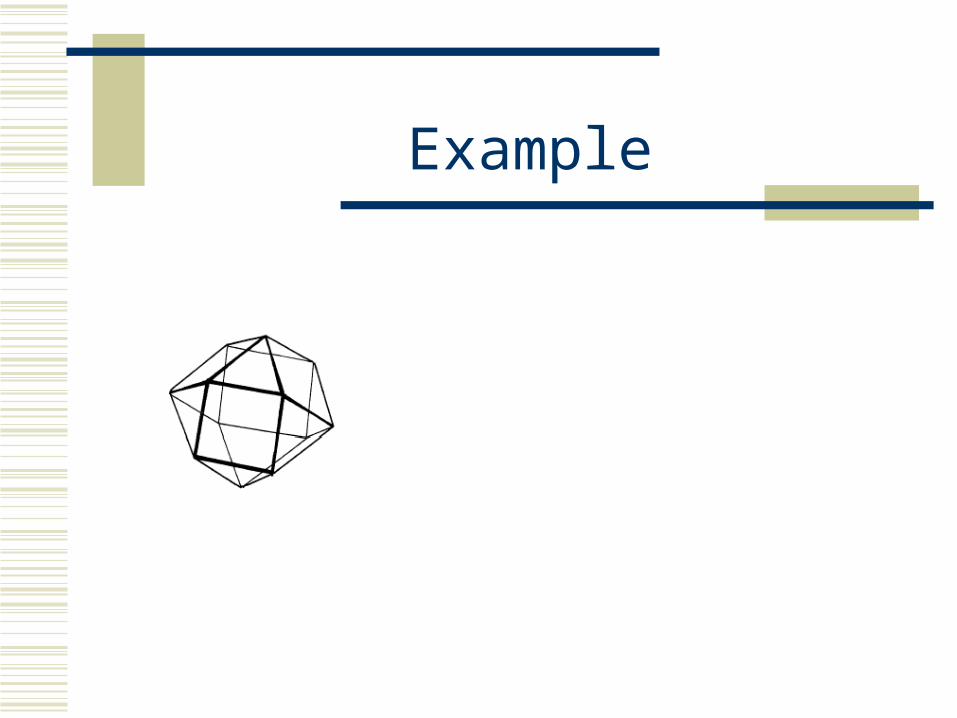
Example

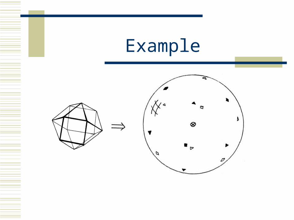
Example

Extended Gaussian Image

Extended to include area of each face. Place point mass on the sphere surface equal to

area of face at the head of each normal. Alternate representation: Scale the normal

proportional to area.

Properties

Face position information is lost. Which faces are connected? As long as the polyhedron is convex, its

extended Gaussian image is unique.Algorithms exist that extract a polyhedron from an

extended Gaussian Image.

Properties

Unaffected by translation Rotation of the object causes an equal

rotation of the extended Gaussian image. Center of mass lies at the origin of the

sphere.

Center of mass property proof

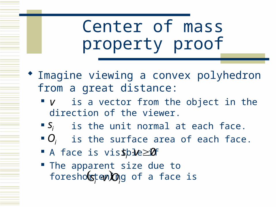
Imagine viewing a convex polyhedron from a great distance: is a vector from the object in the direction of the

viewer. is the unit normal at each face. is the surface area of each face. A face is visible if The apparent size due to foreshortening of a face is

v

is

0vsiiO

ii Ovs

Center of mass property proof

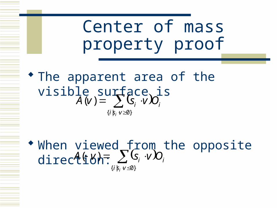
The apparent area of the visible surface is

When viewed from the opposite direction:

}0|{

)(vsi

ii

i

OvsvA

}0|{

)(vsi

ii

i

OvsvA

Center of mass property proof

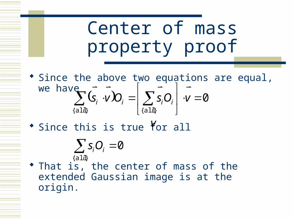
Since the above two equations are equal, we have

Since this is true for all

That is, the center of mass of the extended Gaussian image is at the origin.

0} all{} all{

vOsOvs

iii

iii

v

0} all{

i

iiOs

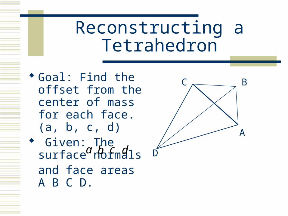
Reconstructing a Tetrahedron

Goal: Find the offset from the center of mass for each face. (a, b, c, d)

Given: The surface normals and face areas A B C D.

D

A

C B

abcd

Reconstructing a Tetrahedron

Tetrahedron property: the distance from the center of mass to a face is ¼ the distance from that face to its opposite vertex.

Start by finding a formula for distance from face of area D to opposite vertex d. The desired distance, d, with be ¼ that.

Repeat for each vertex after doing a cyclical permutation of the variables.

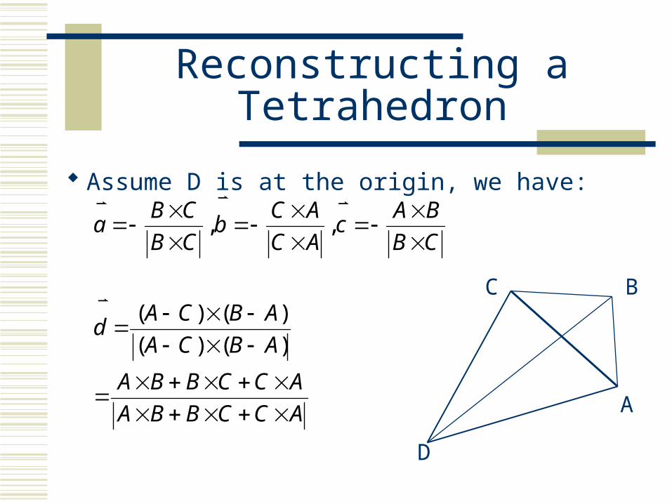
Reconstructing a Tetrahedron

Assume D is at the origin, we have:

ACCBBA

ACCBBA

ABCA

ABCAd

CB

BAc

AC

ACb

CB

CBa

)()(

)()(

,,

D

A

C B

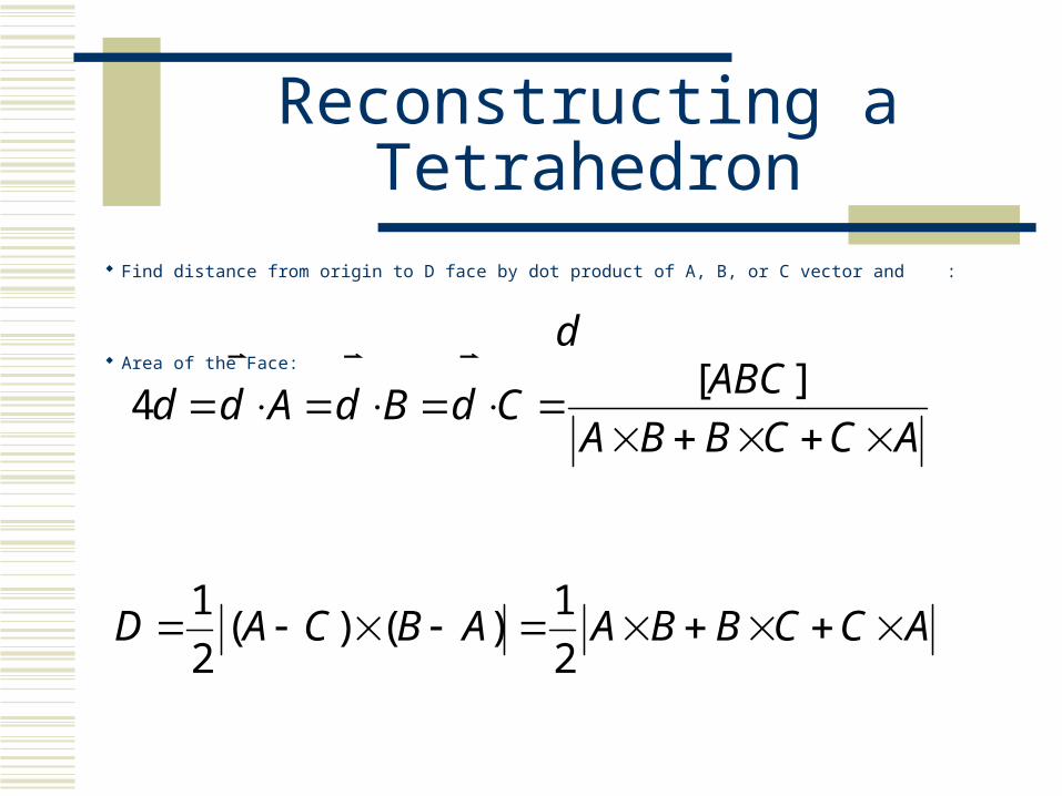
Reconstructing a Tetrahedron

Find distance from origin to D face by dot product of A, B, or C vector and :

Area of the Face:

d

ACCBBA

ABCCdBdAdd

][4

ACCBBAABCAD 2

1)()(

2

1

Reconstructing a Tetrahedron

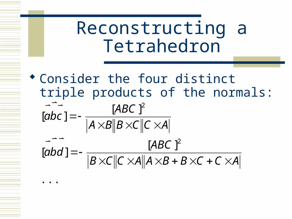
Consider the four distinct triple products of the normals:

...

][][

][][

2

2

ACCBBAACCB

ABCdba

ACCBBA

ABCcba

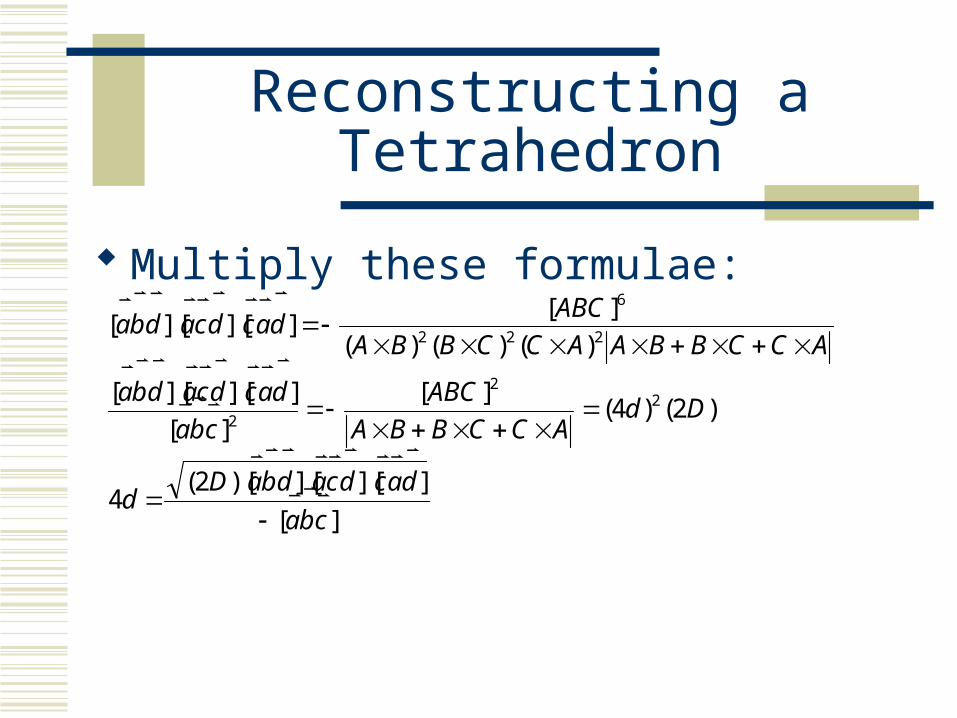
Reconstructing a Tetrahedron

Multiply these formulae:

][

]][][)[2(4

)2()4(][

][

]][][[

)()()(

][]][][[

22

2

222

6

cba

dacdcadbaDd

DdACCBBA

ABC

cba

dacdcadba

ACCBBAACCBBA

ABCdacdcadba

Compute cyclic permutations of each face and use the previous equation to find the 4 distances of each face from the center of mass.

With the normals and distances from the center of mass, create 4 planes. The intersection of the planes creates the

tetrahedron.

Reconstructing a Tetrahedron

Outline

Discrete Case: Convex Polyhedra Continuous Case: Smoothly Curved Objects Discrete Approximation: Needle Maps Tessellation of the Gaussian sphere:

Orientation Histograms Solids of Revolution

Gaussian Image

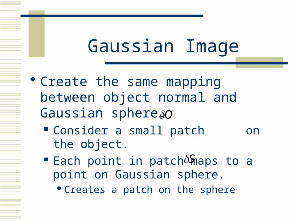
Create the same mapping between object normal and Gaussian sphere. Consider a small patch on the object. Each point in patch maps to a point on Gaussian

sphere.Creates a patch on the sphere

O

S

Gaussian Curvature

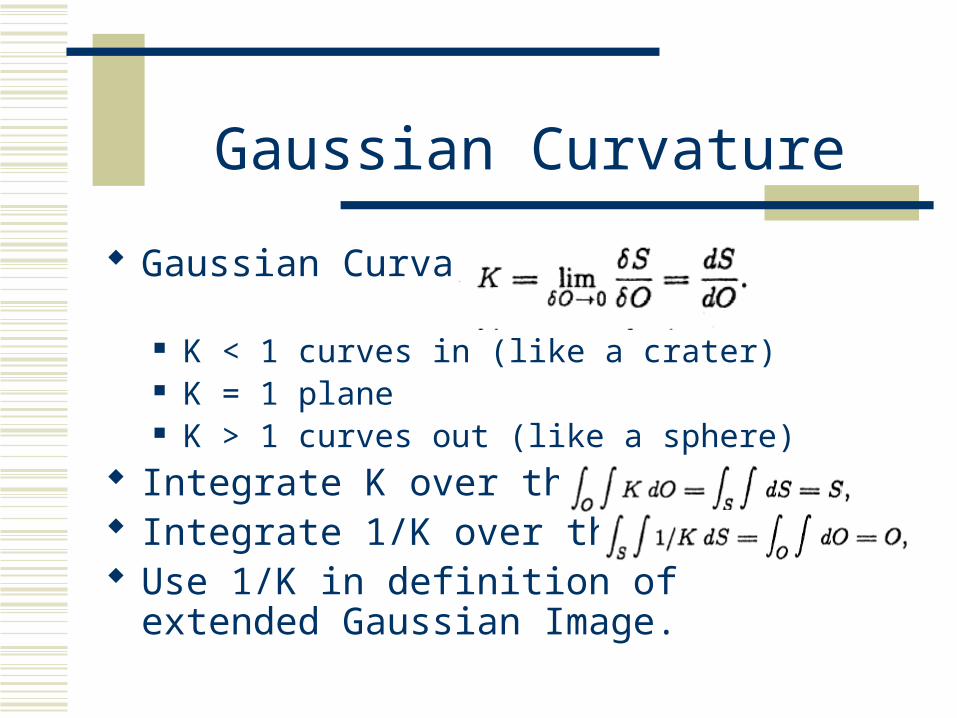
Gaussian Curvature:

K < 1 curves in (like a crater) K = 1 plane K > 1 curves out (like a sphere)

Integrate K over the object: Integrate 1/K over the sphere: Use 1/K in definition of extended Gaussian

Image.

Extended Gaussian Image

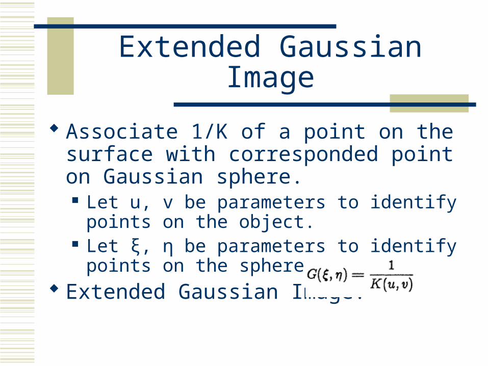
Associate 1/K of a point on the surface with corresponded point on Gaussian sphere. Let u, v be parameters to identify points on the

object. Let ξ, η be parameters to identify points on the

sphere. Extended Gaussian Image:

Properties

Center of mass at origin. Similar proof to discrete case

Total mass of extended Gaussian Image equals surface area of object.

Unaffected by translation Rotation of the object causes an equal

rotation of the extended Gaussian image.

Outline

Discrete Case: Convex Polyhedra Continuous Case: Smoothly Curved Objects Discrete Approximation: Needle Maps Tessellation of the Gaussian sphere:

Orientation Histograms Solids of Revolution

Discrete Approximation

Break the surface into small patches. Create a surface normal for each patch. Consider the polyhedron formed by the

intersection of the planes tangent to each of these normals. Approximation of the original surface.

Discrete Approximation

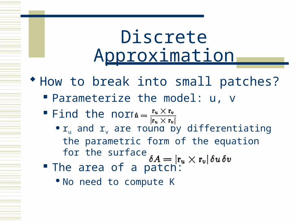
How to break into small patches? Parameterize the model: u, v Find the normal:

ru and rv are found by differentiating the parametric form of the equation for the surface.

The area of a patch:No need to compute K

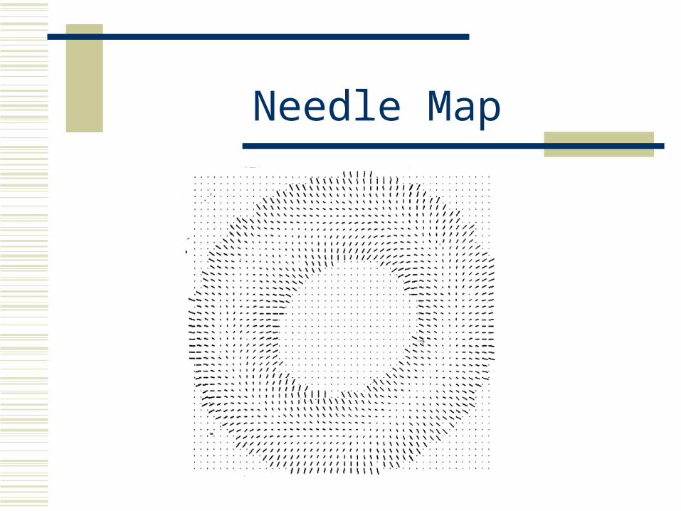
Needle Map

Outline

Discrete Case: Convex Polyhedra Continuous Case: Smoothly Curved Objects Discrete Approximation: Needle Maps Tessellation of the Gaussian sphere:

Orientation Histograms Solids of Revolution

Tessellation

Need a way to represent in a computer Tessellate the Gaussian sphere Create a histogram of orientations

Tessellation Properties

All cells should have the same area. All cells should have the same shape. The cells should have regular shapes that are

compact. The division should be fine enough to provide good

angular resolution. For some rotation, the cells should be brought into

coincidence with themselves.

Simple Case

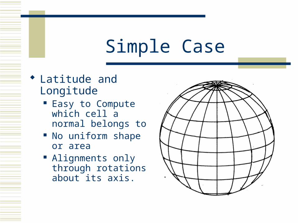
Latitude and Longitude Easy to Compute

which cell a normal belongs to

No uniform shape or area

Alignments only through rotations about its axis.

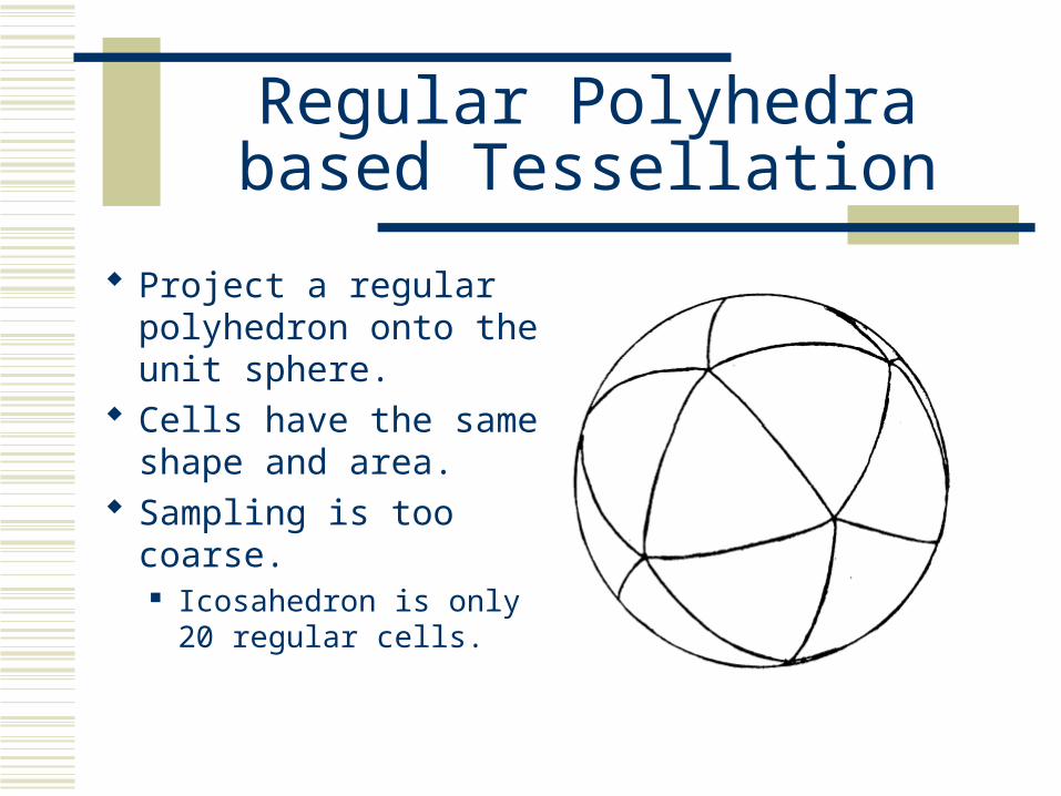
Regular Polyhedra based Tessellation

Project a regular polyhedron onto the unit sphere.

Cells have the same shape and area.

Sampling is too coarse. Icosahedron is only 20

regular cells.

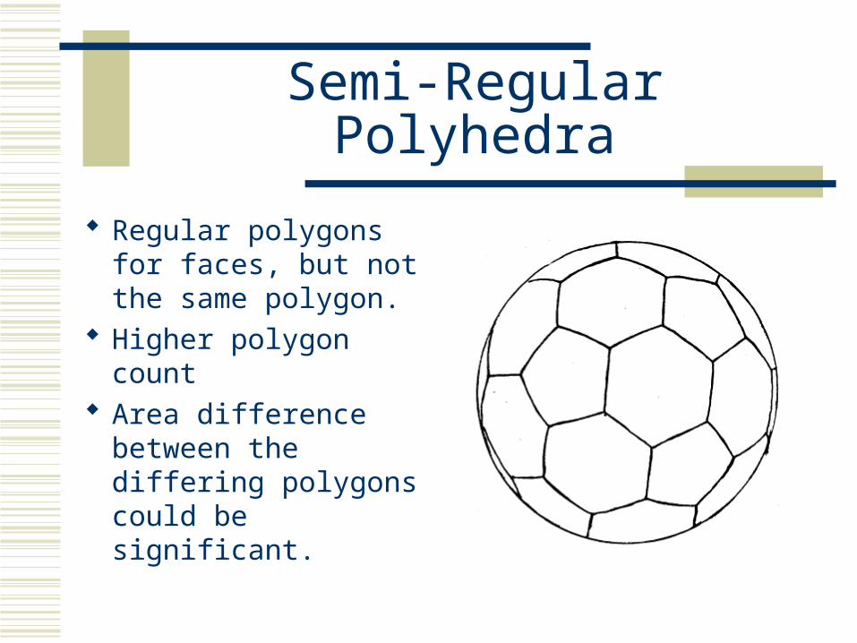
Semi-Regular Polyhedra

Regular polygons for faces, but not the same polygon.

Higher polygon count Area difference

between the differing polygons could be significant.

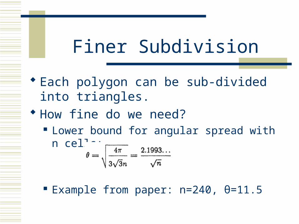
Finer Subdivision

Each polygon can be sub-divided into triangles.

How fine do we need? Lower bound for angular spread with n cells:

Example from paper: n=240, θ=11.5

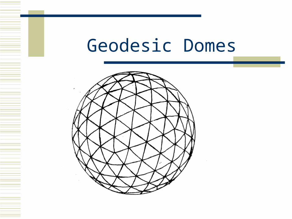
Geodesic Domes

Divide Triangular cells into four smaller triangles. All faces not same area or shape. Allows for arbitrary fineness. Start with pentakis dodecahedron or truncated

icosahedron. Each triangle edge is divided into f sections to create f2

triangles. Desire that f is a power of 2.

Geodesic Domes

Geodesic Domes

Create Histogram by assigning each normal to a cell on the tessellated Gaussian sphere.

Which cell does a normal belong to? Find dot product between given vector and normals from the

original regular polyhedron the dome is based on. Normal belongs to the face giving the greatest result.

Determine which triangle within the face Use the second greatest normal from above.

Proceed as above hierarchically. Binary search through the triangles In practice a lookup table is used

Orientation Histogram

Compute the number of normals in each cell. Count them Create the histogram

Store in computer as simple array. Display graphically with a normal for each

cell or as a grayscale image where the brightness of each cell is determined by the count.

Outline

Discrete Case: Convex Polyhedra Continuous Case: Smoothly Curved Objects Discrete Approximation: Needle Maps Tessellation of the Gaussian sphere:

Orientation Histograms Solids of Revolution

Solids of Revolution

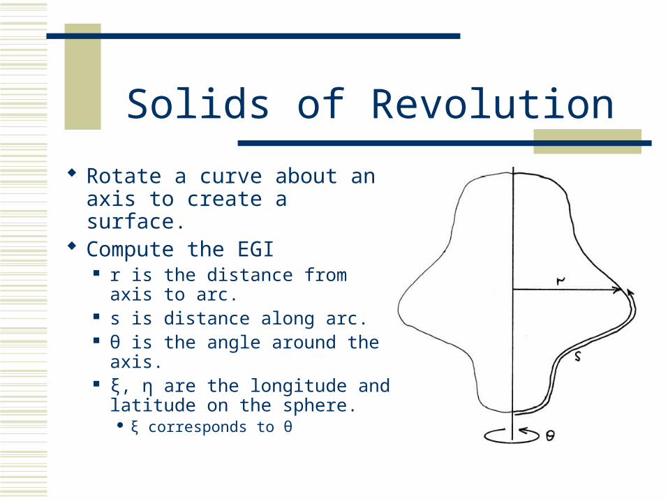
Rotate a curve about an axis to create a surface.

Compute the EGI r is the distance from axis to

arc. s is distance along arc. θ is the angle around the axis. ξ, η are the longitude and

latitude on the sphere. ξ corresponds to θ

Gaussian Curvature

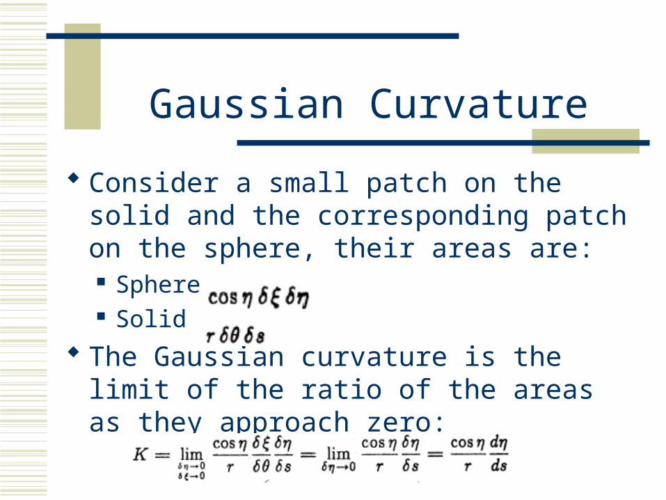
Consider a small patch on the solid and the corresponding patch on the sphere, their areas are: Sphere Solid

The Gaussian curvature is the limit of the ratio of the areas as they approach zero:

Gaussian Curvature

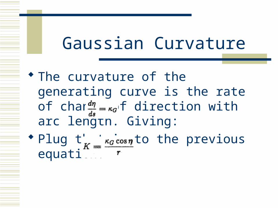
The curvature of the generating curve is the rate of change of direction with arc length. Giving:

Plug that in to the previous equation:

Gaussian Curvature

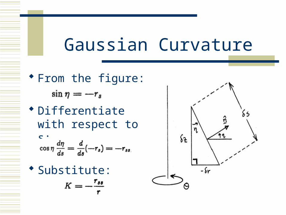
From the figure:

Differentiate with respect to s:

Substitute:

Gaussian Curvature

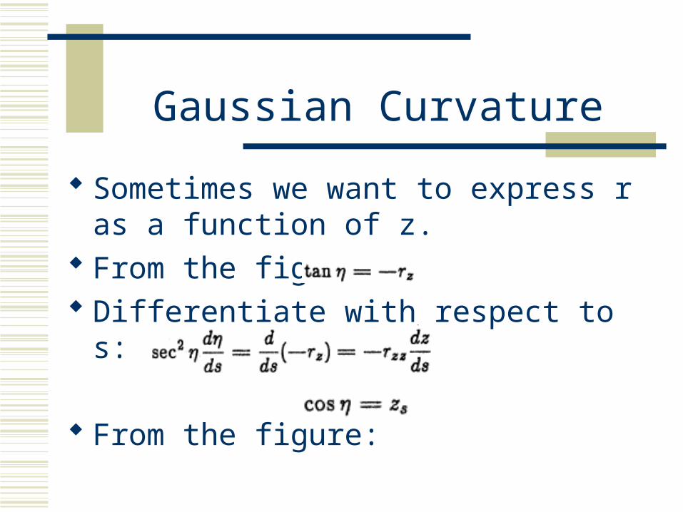
Sometimes we want to express r as a function of z.

From the figure: Differentiate with respect to s:

From the figure:

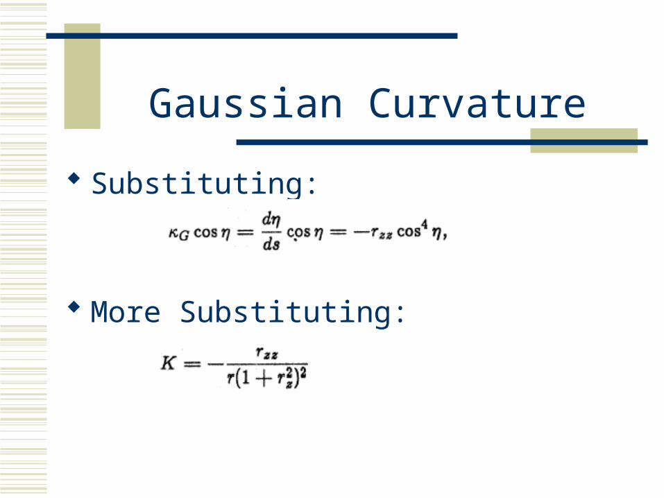
Substituting:

More Substituting:

Gaussian Curvature

Conclusion

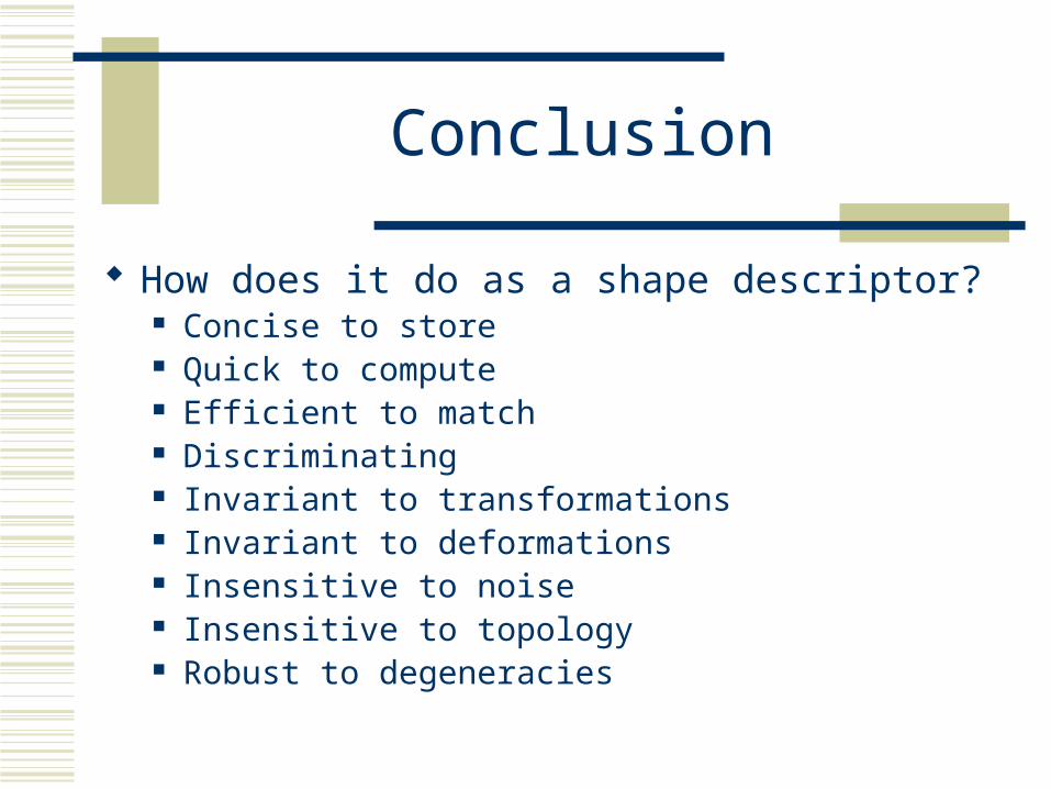
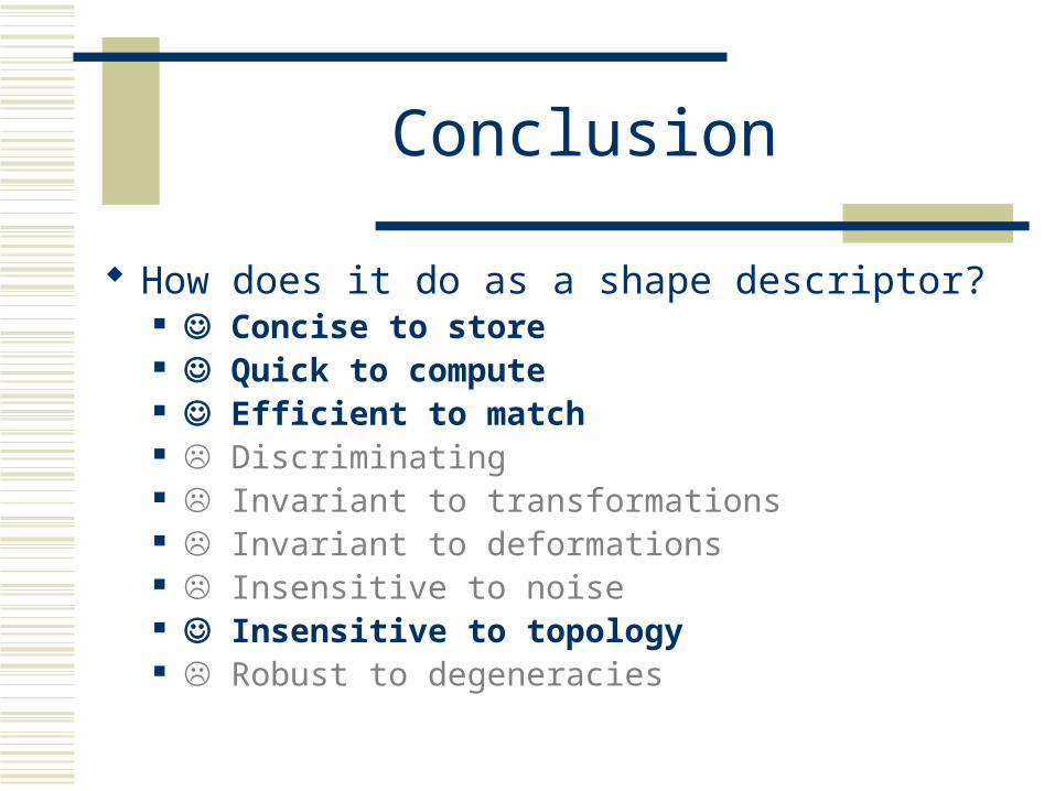
How does it do as a shape descriptor? Concise to store Quick to compute Efficient to match Discriminating Invariant to transformations Invariant to deformations Insensitive to noise Insensitive to topology Robust to degeneracies

Conclusion

How does it do as a shape descriptor? Concise to store Quick to compute Efficient to match Discriminating Invariant to transformations Invariant to deformations Insensitive to noise Insensitive to topology Robust to degeneracies