Statistics and Computing (2020) 30:419–446https://doi.org/10.1007/s11222-019-09886-w

Hilbert space methods for reduced-rank Gaussian process regression

Arno Solin1 · Simo Särkkä2

Received: 31 May 2018 / Accepted: 15 July 2019 / Published online: 5 August 2019© The Author(s) 2019

AbstractThis paper proposes a novel scheme for reduced-rank Gaussian process regression. The method is based on an approximateseries expansion of the covariance function in terms of an eigenfunction expansion of the Laplace operator in a compactsubset ofRd . On this approximate eigenbasis, the eigenvalues of the covariance function can be expressed as simple functionsof the spectral density of the Gaussian process, which allows the GP inference to be solved under a computational costscaling as O(nm2) (initial) and O(m3) (hyperparameter learning) with m basis functions and n data points. Furthermore,the basis functions are independent of the parameters of the covariance function, which allows for very fast hyperparameterlearning. The approach also allows for rigorous error analysis with Hilbert space theory, and we show that the approximationbecomes exact when the size of the compact subset and the number of eigenfunctions go to infinity. We also show that theconvergence rate of the truncation error is independent of the input dimensionality provided that the differentiability orderof the covariance function increases appropriately, and for the squared exponential covariance function it is always boundedby ∼1/m regardless of the input dimensionality. The expansion generalizes to Hilbert spaces with an inner product which isdefined as an integral over a specified input density. The method is compared to previously proposed methods theoreticallyand through empirical tests with simulated and real data.

Keywords Gaussian process regression · Laplace operator · Eigenfunction expansion · Pseudo-differential operator ·Reduced-rank approximation

1 Introduction

Gaussian processes (GPs, Rasmussen and Williams 2006)are powerful tools for nonparametric Bayesian inference andlearning. In GP regression, the model functions f (x) areassumed to be realizations from a Gaussian random processprior with a given covariance function k(x, x′), and learningamounts to solving the posterior process given a set of noisymeasurements y1, y2, . . . , yn at some given test inputs. Thismodel is often written in the form

f ∼ GP(0, k(x, x′)),yi = f (xi ) + εi ,

(1)

B Arno Solinarno.solin@aalto.fi

1 Department of Computer Science, Aalto University,P.O. Box 15400, 00076 Aalto, Finland

2 Department of Electrical Engineering and Automation,Aalto University, P.O. Box 12200, 00076 Aalto, Finland

where εi ∼ N (0, σ 2n ), for i = 1, 2, . . . , n. One of the main

limitations of GPs in machine learning is the computationaland memory requirements that scale as O(n3) and O(n2)

in a direct implementation. This limits the applicability ofGPs when the number of training samples n grows large.The computational requirements arise because in solving theGP regression problem we need to invert the n × n Grammatrix K + σ 2

n I, where Ki j = k(xi , x j ), which is an O(n3)

operation in general.To overcome this problem, over the years, several schemes

have been proposed. They typically reduce the storagerequirements to O(nm) and complexity to O(nm2), wherem < n. Some early methods have been reviewed in Ras-mussen and Williams (2006), and Quiñonero-Candela andRasmussen (2005b) provide a unifying view on severalmeth-ods. From a spectral point of view, several of these methods(e.g., SOR, DTC, VAR, FIC) can be interpreted as modifi-cations to the so-called Nyström method (see Baker 1977;Williams and Seeger 2001), a scheme for approximating theeigenspectrum.

123

420 Statistics and Computing (2020) 30:419–446

For stationary covariance functions, the spectral densityof the covariance function can be employed: In this con-text, the spectral approach has mainly been considered inregular grids, as this allows for the use of FFT-based meth-ods for fast solutions (see Paciorek 2007; Fritz et al. 2009)and more recently in terms of converting GPs to state spacemodels (Särkkä and Hartikainen 2012; Särkkä et al. 2013).Recently, Lázaro-Gredilla et al. (2010) proposed a sparsespectrum method where a randomly chosen set of spectralpoints span a trigonometric basis for the problem.

The methods proposed in this article fall into the classof methods called reduced-rank approximations (see, e.g.,Rasmussen and Williams 2006, Ch. 8) which are based onapproximating the Gram matrix K with a matrix K̃ witha smaller rank m < n. This allows for the use of matrixinversion lemma (Woodbury formula) to speed up the com-putations. It is well known that the optimal reduced-rankapproximation of the Gram (covariance) matrix K withrespect to the Frobenius norm is K̃ = ���T, where� is a diagonal matrix of the leading m eigenvalues ofK and � is the matrix of the corresponding orthonormaleigenvectors (Golub and Van Loan 1996; Rasmussen andWilliams 2006, Ch. 8). Yet, as computing the eigendecom-position is an O(n3) operation, this provides no remedy assuch.

In this work, we propose a novel method for obtainingapproximate eigendecompositions of covariance functionsin terms of an eigenfunction expansion of the Laplace oper-ator in a compact subset of Rd . The method is based oninterpreting the covariance function as the kernel of a pseudo-differential operator (Shubin 1987) and approximating itusing Hilbert space methods (Courant and Hilbert 2008;Showalter 2010). This results in a reduced-rank approxima-tion for the covariance function, where the basis functionsare independent of the covariance functions and its param-eters. We also show that the approximation converges tothe exact solution in well-defined conditions, analyze itsconvergence rate and provide theoretical and experimen-tal comparisons to existing state-of-the-art methods. Thispath has not been explored in GP regression context before,although the approach is related to the Fourier feature meth-ods (Hensman et al. 2018) and stochastic partial differentialequation-based methods recently introduced to spatial statis-tics and GP regression (Lindgren et al. 2011; Särkkä andHartikainen 2012; Särkkä et al. 2013) as well as to classicalworks in the spectral representations of stochastic processes(Loève 1963;VanTrees 1968;Adler 1981; Cramér andLead-better 2013) and spline interpolation (Wahba 1978, 1990;Kimeldorf and Wahba 1970). Recently, the scalable eigen-decomposition approach has also been tackled by variousstructure exploiting methods (building on the work by Wil-son and Nickisch 2015) and extended to methods exploitingGPU computations.

This paper is structured as follows: InSect. 2,wederive theapproximative series expansion of the covariance functions.Section 3 is dedicated to applying the approximation schemeto GP regression and providing details of the computationalbenefits.We provide a detailed analysis of the convergence ofthe method in Sect. 4. Sections 5 and 6 provide comparisonsto existing methods, the former from amore theoretical pointof view, whereas the latter contains examples and compara-tive evaluation on several datasets. Finally, the properties ofthe method are summarized and discussed in Sect. 7.

2 Approximating the covariance function

In this section, we start by stating the assumptions andproperties of the class of covariance functions that we areconsidering and show how a homogenous covariance func-tion can be considered as a pseudo-differential operatorconstructed as a series of Laplace operators. Then we showhow the pseudo-differential operators can be approximatedwith Hilbert space methods on compact subsets of Rd or viainner products with integrable weight functions and discussconnections to Sturm–Liouville theory.

2.1 Spectral densities of homogeneous andisotropic Gaussian processes

In this work, it is assumed that the covariance function ishomogeneous (stationary), which means that the covariancefunction k(x, x′) is actually a function of r = x − x′ only.This means that the covariance structure of the model func-tion f (x) is the same regardless of the absolute position inthe input space (cf. Rasmussen andWilliams 2006, Ch. 4). Inthis case, the covariance function can be equivalently repre-sented in terms of the spectral density. This results from theBochner’s theorem (see, e.g., Akhiezer and Glazman 1993;DaPrato andZabczyk 1992)which states that a bounded con-tinuous positive definite function k(r) can be represented as

k(r) = 1

(2π)d

∫exp

(iωTr

)μ(dω), (2)

where μ is a positive measure.If the measure μ(ω) has a density, it is called the spec-

tral density S(ω) corresponding to the covariance functionk(r). This gives rise to the Fourier duality of covariance andspectral density, which is known as the Wiener–Khintchintheorem (Rasmussen and Williams 2006, Ch. 4), giving theidentities

k(r) = 1

(2π)d

∫S(ω) eiω

Tr dω,

S(ω) =∫

k(r) e−iωTr dr.(3)

123

Statistics and Computing (2020) 30:419–446 421

From these identities, it is easy to see that if the covariancefunction is isotropic, that is, it only depends on the Euclideannorm ‖r‖ such that k(r) � k(‖r‖), then the spectral densitywill also only depend on the norm of ω such that we canwrite S(ω) � S(‖ω‖). In the following, we assume that theconsidered covariance functions are indeed isotropic, but theapproach can be generalized to more general homogenouscovariance functions.

2.2 The covariance operator as a pseudo-differentialoperator

Associated to each covariance function k(x, x′), we can alsodefine a covariance operator K as follows:

K φ =∫

k(·, x′) φ(x′) dx′. (4)

Note that because the covariance function is homogeneous,this can also be written as a convolution. As we show inthe next section, this interpretation allows us to approxi-mate the covariance operator using Hilbert space methodswhich are typically used for approximating differential andpseudo-differential operators in the context of partial dif-ferential equations (Showalter 2010). When the covariancefunction is homogenous, the corresponding operator will betranslation invariant thus allowing for Fourier representationas a transfer function. This transfer function is just the spec-tral density of the Gaussian process.

Consider an isotropic covariance function k(x, x′) �k(‖r‖) (recall that ‖·‖ denotes the Euclidean norm). Thespectral density of the Gaussian process and thus the transferfunction corresponding to the covariance operator will nowhave the form S(‖ω‖). We can formally write it as a functionof ‖ω‖2 such that

S(‖ω‖) = ψ(‖ω‖2). (5)

Assume that the spectral density S(·) and hence ψ(·) havethe following polynomial expansion:

ψ(‖ω‖2) = a0 + a1‖ω‖2 + a2(‖ω‖2)2 + a3(‖ω‖2)3 + · · · .

(6)

This can be ensured, for example, by requiring that ψ(·) isan analytic function. Thus we also have

S(‖ω‖) = a0+a1‖ω‖2+a2(‖ω‖2)2+a3(‖ω‖2)3+· · · . (7)

Recall that the transfer function corresponding to the Laplaceoperator ∇2 is −‖ω‖2 in the sense that for a regular enoughfunction f we have

F [∇2 f ](ω) = −‖ω‖2F [ f ](ω), (8)

whereF [·] denotes the Fourier transform of its argument. Ifwe take the inverse Fourier transform of (7), we get the fol-lowing representation for the covariance operator K, whichdefines a pseudo-differential operator (Shubin 1987) as a for-mal series of Laplace operators:

K = a0 + a1(−∇2) + a2(−∇2)2 + a3(−∇2)3 + · · · . (9)

In the next section, we will use this representation to form aseries expansion approximation for the covariance function.

2.3 Hilbert space approximation of the covarianceoperator

We will now form a Hilbert space approximation for thepseudo-differential operator defined by (9). Let Ω ⊂ R

d bea compact set and consider the eigenvalue problem for theLaplace operators with Dirichlet boundary conditions (wecould use other boundary conditions as well):

{−∇2φ j (x) = λ j φ j (x), x ∈ Ω,

φ j (x) = 0, x ∈ ∂Ω.(10)

Let us now assume that we have selected ∂Ω to be suffi-ciently smooth, for example, a hypercube or hypersphere,so that the eigenfunctions and eigenvalues exist. Because−∇2 is a positive definite Hermitian operator, the set ofeigenfunctions φ j (·) is orthonormal with respect to the innerproduct

〈 f , g〉 =∫

Ω

f (x) g(x) dx (11)

that is,

∫Ω

φi (x) φ j (x) dx = δi j , (12)

and all the eigenvalues λ j are real and positive. The neg-ative Laplace operator can then be assigned the formalkernel

l(x, x′) =∑

j

λ j φ j (x) φ j (x′) (13)

in the sense that

−∇2 f (x) =∫

l(x, x′) f (x′) dx′, (14)

for sufficiently (weakly) differentiable functions f in thedomain Ω assuming Dirichlet boundary conditions.

123

422 Statistics and Computing (2020) 30:419–446

0 5�

ν → ∞ν = 72ν = 5

2ν = 32ν = 1

2 Exactm = 12m = 32m = 64m = 128

Fig. 1 Approximations to covariance functions of the Matérn class ofvarious degrees of smoothness; ν = 1/2 corresponds to the exponentialOrnstein–Uhlenbeck covariance function and ν → ∞ to the squared

exponential (exponentiated quadratic) covariance function. Approxi-mations are shown for 12, 32, 64, and 128 eigenfunctions

If we consider the formal powers of this representation,due to orthonormality of the basis, we can write the arbitraryoperator power s = 1, 2, . . . of the kernel as

ls(x, x′) =∑

j

λsj φ j (x) φ j (x′). (15)

This is again to be interpreted to mean that

(−∇2)s f (x) =∫

ls(x, x′) f (x′) dx′, (16)

for regular enough functions f and in the current domainwith the assumed boundary conditions.

This implies that on the domainΩ , assuming the boundaryconditions, we also have

[a0 + a1(−∇2) + a2(−∇2)2 + · · ·

]f (x)

=∫ [

a0 + a1 l1(x, x′) + a2 l2(x, x′) + · · ·]

f (x′) dx′.

(17)

The left hand side is just K f via (9), on the domain withthe boundary conditions, and thus, by comparing to (4) andusing (15), we can conclude that

k(x, x′) ≈ a0 + a1 l1(x, x′) + a2 l2(x, x′) + · · ·=

∑j

[a0 + a1 λ1j + a2 λ2j + · · ·

]φ j (x) φ j (x′),

(18)

which is only an approximation to the covariance functiondue to restriction of the domain to Ω and the boundary con-ditions. By letting ‖ω‖2 = λ j in (7), we now obtain

S(√

λ j ) = a0 + a1λ1j + a2λ

2j + · · · (19)

and substituting this into (18) leads to the approximation

k(x, x′) ≈∑

j

S(√

λ j ) φ j (x) φ j (x′), (20)

where S(·) is the spectral density of the covariance function,λ j is the j th eigenvalue and φ j (·) the eigenfunction of theLaplace operator in a given domain. These expressions tendto be simple closed-form expressions.

The right-hand side of (20) is very easy to evaluate,because it corresponds to evaluating the spectral density atthe square roots of the eigenvalues and multiplying themwith the eigenfunctions of the Laplace operator. Becausethe eigenvalues of the Laplace operator are monotonicallyincreasing with j and for bounded covariance functions thespectral density goes to zero fast with higher frequencies,we can expect to obtain a good approximation of the right-hand side by retaining only a finite number of terms in theseries. However, even with an infinite number of terms thisis only an approximation, because we assumed a compactdomain with boundary conditions. The approximation canbe, though, expected to be good at the input values which arenot near the boundary of Ω , where the Laplacian was takento be zero.

As an example, Fig. 1 showsMatérn covariance functionsof various degrees of smoothness ν (see, e.g., Rasmussenand Williams 2006, Ch. 4) and approximations for differ-ent numbers of basis functions in the approximation. Thebasis consists of the eigenfunctions of the Laplacian in(10) with Ω = [− L, L] which gives the eigenfunctionsφ j (x) = L−1/2 sin(π j(x + L)/(2L)) and the eigenvaluesλ j = (π j/(2L))2. In the figure, we have set L = 1 and = 0.1. For the squared exponential, the approximation isindistinguishable from the exact curve already at m = 12,whereas the less smooth functions require more terms.

123

Statistics and Computing (2020) 30:419–446 423

2.4 Inner product point of view

Instead of considering a compact bounded set Ω , we canconsider the same approximation in terms of an inner productdefined by an input density (Williams and Seeger 2000). Letthe inner product be defined as

〈 f , g〉 =∫

f (x) g(x) w(x) dx, (21)

where w(x) is some positive weight function such that∫w(x) dx < ∞. In terms of this inner product, we define

the operator

K f =∫

k(·, x) f (x) w(x) dx. (22)

This operator is self-adjoint with respect to the inner product,〈K f , g〉 = 〈 f ,Kg〉, and according to the spectral theoremthere exists an orthonormal set of basis functions and pos-itive constants, {ϕ j (x), γ j | j = 1, 2, . . .}, that satisfies theeigenvalue equation

(Kϕ j )(x) = γ j ϕ j (x). (23)

Thus k(x, x′) has the series expansion

k(x, x′) =∑

j

γ j ϕ j (x) ϕ j (x′). (24)

Similarly, we also have the Karhunen–Loeve expansion for asample function f (x) with zero mean and the above covari-ance function:

f (x) =∑

j

f j ϕ j (x), (25)

where f j s are independent zero mean Gaussian random vari-ables with variances γ j (see, e.g., Lenk 1991).

For the negative Laplacian, the corresponding definitionis

D f = −∇2[ f w], (26)

which implies

〈D f , g〉 = −∫

f (x) w(x)∇2[g(x) w(x)] dx, (27)

and the operator defined by (26) can be seen to be self-adjoint. Again, there exists an orthonormal basis {φ j (x)| j =1, 2, . . .} and positive eigenvalues λ j which satisfy the eigen-value equation

(D φ j )(x) = λ j φ j (x). (28)

Thus the kernel ofD has a series expansion similar to Eq. (13)and thus an approximation can be given in the same form asin Equation (20). In this case, the approximation error comesfrom approximating the Laplace operator with the smootheroperator,

∇2 f ≈ ∇2[ f w], (29)

which is closely related to assumption of an input densityw(x) for the Gaussian process. However, when the weightfunctionw(·) is close to constant in the area where the inputspoints are located, the approximation is accurate.

2.5 Connection to Sturm–Liouville theory

The presented methodology is also related to the Sturm–Liouville theory arising in the theory of partial differentialequations (Courant and Hilbert 2008). When the input x isscalar, the eigenvalue problem in Eq. (23) can be written inSturm–Liouville form as follows:

− d

dx

[w2(x)

dφ j (x)

dx

]− w(x)

d2w(x)

dx2φ j (x)

= λ j w(x) φ j (x).

(30)

The above equation can be solved for φ j (x) and λ j usingnumerical methods for Sturm–Liouville equations. Also notethat if we select w(x) = 1 in a finite set, we obtain theequation − d2/ dx2 φ j (x) = λ j φ j (x) which is compatiblewith the results in the previous section.

We consider the casewhere x ∈ Rd andw(x) is symmetric

around the origin and thus is only a function of the normr = ‖x‖ (i.e. has the form w(r)). The Laplacian in sphericalcoordinates is

∇2 f = 1

rd−1

∂

∂r

(rd−1 ∂ f

∂r

)+ 1

r2�Sd−1 f , (31)

where �Sd−1 is the Laplace–Beltrami operator on Sd−1. Letus assume that φ j (r , ξ) = h j (r) g(ξ), where ξ denotesthe angular variables. After some algebra, writing theequations into Sturm–Liouville form yields for the radialpart

− d

dr

(w2(r) r

dh j (r)

dr

)

−(dw(r)

drw(r) + d2w(r)

dr2w(r) r

)h j (r)

= λ j w(r) r h j (r), (32)

and �Sd−1g(ξ) = 0 for the angular part. The solutions tothe angular part are the Laplace’s spherical harmonics. Note

123

424 Statistics and Computing (2020) 30:419–446

Fig. 2 Approximate random draws of Gaussian processes with the Matérn covariance function on the hull of a unit sphere. The color scale andradius follow the process

that if we assume that we have w(r) = 1 on some areaof finite radius, the first equation becomes (when d > 1):

r2d2h j (r)

dr2+ r

dh j (r)

dr+ r2 λ j h j (r) = 0. (33)

Figure 2 shows example Gaussian random field draws ona unit sphere, where the basis functions are the Laplacespherical harmonics and the covariance functions of theMatérn class with different degrees of smoothness ν. Ourapproximation is straight-forward to apply in any domain,where the eigendecomposition of the Laplacian can beformed.

3 Application of themethod to GPregression

In this section, we show how the approximation (20) can beused in Gaussian process regression. We also write down theexpressions needed for hyperparameter learning and discussthe computational requirements of the methods.

3.1 Gaussian process regression

GPregression is usually formulated as predicting anunknownscalar output f (x∗) associated with a known input x∗ ∈ R

d ,given a training data set D = {(xi , yi )|i = 1, 2, . . . , n}. Themodel functions f are assumed to be realizations of a Gaus-sian random process prior and the observations corrupted byGaussian noise:

f ∼ GP(0, k(x, x′))yi = f (xi ) + εi ,

(34)

where εi ∼ N (0, σ 2n ). For notational simplicity, the func-

tions in the above model are a priori zero mean and themeasurement errors are independentGaussian, but the results

of this paper can be easily generalized to arbitrary meanfunctions and dependent Gaussian errors. The direct solu-tion to the GP regression problem (34) gives the predictionsp( f (x∗)|D) = N ( f (x∗)|E[ f (x∗)],V[ f (x∗)]). The condi-tional mean and variance can be computed in closed form as(see, e.g., Rasmussen and Williams 2006, p. 17)

E[ f (x∗)] = kT∗(K + σ 2n I)

−1y,

V[ f (x∗)] = k(x∗, x∗) − kT∗(K + σ 2n I)

−1k∗,(35)

where Ki j = k(xi , x j ), k∗ is an n-dimensional vector withthe i th entry being k(x∗, xi ), and y is a vector of the n obser-vations.

In order to avoid the n×n matrix inversion in (35), we usethe approximation scheme presented in the previous sectionand project the process to a truncated set of m basis functionsof the Laplacian as given in Eq. (20) such that

f (x) ≈m∑

j=1

f j φ j (x), (36)

where f j ∼ N (0, S(√

λ j )). We can then form an approxi-mate eigendecomposition of the matrix K ≈ ���T, where� is a diagonal matrix of the leading m approximate eigen-values such that � j j = S(

√λ j ), j = 1, 2, . . . , m. Here S(·)

is the spectral density of the Gaussian process and λ j the j theigenvalue of the Laplace operator. The corresponding eigen-vectors in the decomposition are given by the eigenvectorsφ j (x) of the Laplacian such that �i j = φ j (xi ).

Using the matrix inversion lemma, we rewrite (35) as fol-lows:

E[ f∗] ≈ φT∗(�T� + σ 2n �−1)−1�Ty,

V[ f∗] ≈ σ 2n φT∗(�T� + σ 2

n �−1)−1φ∗,(37)

123

Statistics and Computing (2020) 30:419–446 425

where φ∗ is anm-dimensional vector with the j th entry beingφ j (x∗). Thus, when the size of the training set is higher thanthe number of required basis functions n > m, the use of thisapproximation is advantageous.

3.2 Learning the hyperparameters

A common way to learn the hyperparameters θ of the covari-ance function (suppressed earlier in the notation for brevity)and the noise variance σ 2

n is bymaximizing themarginal like-lihood function (Rasmussen andWilliams 2006; Quiñonero-Candela and Rasmussen 2005a). Let Q = K + σ 2

n I for thefull model, then the negative log marginal likelihood and itsderivatives are

L = 1

2log |Q| + 1

2yTQ−1y + n

2log(2π), (38)

∂L∂θk

= 1

2Tr

(Q−1 ∂Q

∂θk

)− 1

2yTQ−1 ∂Q

∂θkQ−1y, (39)

∂L∂σ 2

n= 1

2Tr

(Q−1

)− 1

2yTQ−1Q−1y, (40)

and they can be combined with a conjugate gradient opti-mizer. The problem in this case is the inversion ofQ, which isan n×n matrix.And thus each step of running the optimizer isO(n3). For our approximation scheme, let Q̃ = ���T+σ 2

n I.Now replacing Q with Q̃ in the above expressions gives usthe following:

L̃ = 1

2log |Q̃| + 1

2yTQ̃−1y + n

2log(2π), (41)

∂L̃∂θk

= 1

2

∂ log |Q̃|∂θk

+ 1

2

∂yTQ̃−1y∂θk

, (42)

∂L̃∂σ 2

n= 1

2

∂ log |Q̃|∂σ 2

n+ 1

2

∂yTQ̃−1y∂σ 2

n, (43)

where for the terms involving log |Q̃|:

log |Q̃| = (n − m) log σ 2n + log |Z|

+m∑

j=1

log S(√

λ j ), (44)

∂ log |Q̃|∂θk

=m∑

j=1

S(√

λ j )−1 ∂S(

√λ j )

∂θk

− σ 2n Tr

(Z−1�−2 ∂�

∂θk

), (45)

∂ log |Q̃|∂σ 2

n= n − m

σ 2n

+ Tr(Z−1�−1

), (46)

and for the terms involving Q̃−1:

yTQ̃−1y = 1

σ 2n

(yTy − yT�Z−1�Ty

), (47)

∂yTQ̃−1y∂θk

= − yT�Z−1(

�−2 ∂�

∂θk

)Z−1�Ty, (48)

∂yTQ̃−1y∂σ 2

n= 1

σ 2nyT�Z−1�−1Z−1�Ty − 1

σ 4nyTy, (49)

where Z = σ 2n �−1 + �T�. For efficient implementation,

matrix-to-matrix multiplications can be avoided in manycases, and the inversion of Z can be carried out throughCholesky factorization for numerical stability. This factor-ization (LLT = Z) can also be used for the term log |Z| =2

∑j logL j j , and Tr

(Z−1�−1) = ∑

j 1/(Z j j� j j ) can beevaluated by element-wise multiplication.

Once the marginal likelihood and its derivatives are avail-able, it is also possible to use other methods for parameterinference such as Markov chain Monte Carlo methods (Liu2001; Brooks et al. 2011) including Hamiltonian MonteCarlo (HMC,Duane et al. 1987;Neal 2011) aswell as numer-ous others.

3.3 Discussion on the computational complexity

As can be noted from Eq. (20), the basis functions in thereduced-rank approximation do not depend on the hyperpa-rameters of the covariance function. Thus it is enough tocalculate the product �T� only once, which means that themethod has a overall asymptotic computational complexityof O(nm2). After this initial cost, evaluating the marginallikelihood and the marginal likelihood gradient is an O(m3)

operation—which in practice comes from the Cholesky fac-torization of Z on each step.

If the number of observations n is so large that storing then ×m matrix� is not feasible, the computations of�T� canbe carried out in blocks. Storing the evaluated eigenfunctionsin � is not necessary, because the φ j (x) are closed-formexpressions that canbe evaluatedwhennecessary. In practice,it might be preferable to cache the result of �T� (causinga memory requirement scaling as O(m2)), but this is notrequired.

The computational complexity of conventional sparse GPapproximations typically scale as O(nm2) in time for eachstep of evaluating the marginal likelihood. The scaling indemand of storage isO(nm). This comes from the inevitablecost of re-evaluating all results involving the basis functionson each step and storing the matrices required for doingthis. This applies to all the methods that will be discussedin Sect. 5, with the exception of SSGP, where the storagedemand can be relaxed by re-evaluating the basis functionson demand.

We can also consider the rather restricting, but in certainapplications often encountered case, where the measure-

123

426 Statistics and Computing (2020) 30:419–446

ments are constrained to a regular grid. This causes theproduct of the orthonormal eigenfunction matrices �T� tobe diagonal, avoiding the calculation of the matrix inversealtogether. This relates to the FFT-based methods for GPregression (Paciorek 2007; Fritz et al. 2009), and the projec-tions to the basis functions can be evaluated by fast Fouriertransform in O(n log n) time complexity.

3.4 Inverse problems and latent force models

We can also use the methodology to models of the form

f (x) ∼ GP(0, k(x, x′)),yi = (H f )(xi ) + εi ,

(50)

where H is a linear operator acting on functions dependingon the x variable. This kind of models appear both in inverseproblems literature and machine learning (see, e.g., Taran-tola 2004; Kaipio and Somersalo 2005; Särkkä 2011). TheGaussian process regression solution now becomes

E[ f (x∗)] = kT∗h(Kh + σ 2n I)

−1y,

V[ f (x∗)] = k(x∗, x∗) − kT∗h(Kh + σ 2n I)

−1k∗h,(51)

where [Kh]i j = (HH′ k)(xi , x j ), the i th entry of vector k∗h

is (H′ k(x∗, ·))(xi ), and y is the vector of observations. HereH′ denotes that the operator is applied to the second variablex′ of the argument. With the series expansion (20), we caneasily approximate

(HH′ k)(x, x′) ≈∑

j

S(√

λ j ) (H φ j )(x) (H φ j )(x′),

(H′ k(x∗, ·))(x′) ≈∑

j

S(√

λ j ) φ j (x∗) (H φ j )(x′). (52)

After applying the matrix inversion lemma (51) becomes

E[ f∗] ≈ φT∗(�̃T�̃ + σ 2

n �−1)−1�̃Ty,

V[ f∗] ≈ σ 2n φT∗(�̃

T�̃ + σ 2

n �−1)−1φ∗,(53)

where �̃i j = (Hφ j )(xi ) and φ∗ is as defined in (37). Thehyperparameter estimation methods discussed in Sect. 3.2can also be easily extended to this case.

Another (related) type of model is the following modelarising in the context of latent force models (LFM, Álvarezet al. 2013)

f (x) ∼ GP(0, k(x, x′)),Lg = f ,

yi = g(xi ) + εi ,

(54)

where L is a linear operator. We can now write H = L−1,where L−1 is the Green’s operator associated with the oper-ator L, and hence, the model becomes a special case of (50).The approximation to the operator L−1 on the given basiscan be easily formed by using, for example, by projectingit onto the basis or by using point collocation. A particu-larly simple cases arises when the operator itself containsof Laplace operators, for example, when it has the formL = ∇2. In that case, the projection of the operator becomesdiagonal.

4 Convergence analysis

In this section, we analyze the convergence of the proposedapproximationwhen the size of the domainΩ and the numberof terms in the series grows to infinity. We start by analyzinga univariate problem in the domain Ω = [−L, L] and withDirichlet boundary conditions and then generalize the resultto d-dimensional cubes Ω = [−L1, L1] × · · · × [−Ld , Ld ].Then we analyze the truncation error as function of the num-ber of terms in the series. We also discuss how the analysiscould be extended to other types of basis functions.

4.1 Univariate Dirichlet case

In the univariate case, the m-term approximation has theform

k̃m(x, x ′) =m∑

j=1

S(√

λ j ) φ j (x) φ j (x ′), (55)

where the eigenfunctions and eigenvalues for j = 1, 2, . . .are:

φ j (x) = 1√L

sin

(π j (x + L)

2L

)and λ j =

(π j

2L

)2

.

(56)

The true covariance function k(x, x ′) is assumed to bestationary and have a spectral density with the followingproperties. It is uniformly bounded S(ω) = B < ∞ and hasat least one bounded derivative |S′(ω)| = D < ∞ on ω > 0.The following integrals are also assumed to be bounded:∫ ∞0 S(ω) dω = A < ∞ and

∫ ∞0 |S′(ω)| dω = C < ∞. We

also assume that our training and test sets are constrainedin the area [− L̃, L̃], where L̃ < L , and thus we are onlyinterested in the case x, x ′ ∈ [− L̃, L̃]. For the purposes ofanalysis, we also assume that L is bounded below by a con-stant.

The univariate convergence result can be summarized asthe following theorem which is proved in “Appendix A.2.”

123

Statistics and Computing (2020) 30:419–446 427

Theorem 1 There exists a constant E (independent of m, x,and x ′) such that

∣∣k(x, x ′) − k̃m(x, x ′)∣∣ ≤ E

L+ 2

π

∫ ∞π m2L

S(ω) dω, (57)

which in turn implies that uniformly

limL→∞

[lim

m→∞ k̃m(x, x ′)]

= k(x, x ′). (58)

Remark 2 Note that we cannot simply exchange the orderof the limits in the above theorem. However, the theoremdoes ensure the convergence of the approximation in the jointlimit m, L → ∞ provided that we add terms to the seriesfast enough such that m/L → ∞. That is, in this limit, theapproximation k̃m(x, x ′) converges uniformly to k(x, x ′).

As such, the results above only ensure the convergence ofthe prior covariance functions. However, it turns out that thisalso ensures the convergence of the posterior as is summa-rized in the following corollary.

Corollary 3 Because the Gaussian process regression equa-tions only involve point-wise evaluations of the kernels, italso follows that the posterior mean and covariance func-tions converge uniformly to the exact solutions in the limitm, L → ∞.

Proof Analogous to proof of Theorem 2.2 in Särkkä andPiché (2014). ��

4.2 Multivariate Cartesian Dirichlet case

In order to generalize the results from the previous section,we turn our attention to a d-dimensional inputs space withrectangular domain Ω = [− L1, L1] × · · · × [− Ld , Ld ]with Dirichlet boundary conditions. In this case, we considera truncated m = m̂d term approximation of the form

k̃m(x, x′)

=m̂∑

j1,..., jd=1

S(√

λ j1,..., jd ) φ j1,..., jd (x) φ j1,..., jd (x′) (59)

with the eigenfunctions and eigenvalues

φ j1,..., jd (x) =d∏

k=1

1√Lk

sin

(π jk (xk + Lk)

2Lk

)(60)

and

λ j1,..., jd =d∑

k=1

(π jk2Lk

)2

. (61)

The true covariance function k(x, x′) is assumed to be homo-geneous (stationary) and have a spectral density S(ω) whichsatisfies the one-dimensional assumptions listed in the pre-vious section in each variable. Furthermore, we assume thatthe training and test sets are contained in the d-dimensionalcube [−L̃, L̃]d and that Lks are bounded from below.

The following result for this d-dimensional case is provedin “Appendix A.3.”

Theorem 4 There exists a constant E (independent of m, d,x, and x′) such that

∣∣k(x, x′) − k̃m(x, x′)∣∣ ≤ E d

L+ 1

πd

∫‖ω‖≥ π m̂

2L

S(ω) dω,

(62)

where L = mink Lk, which in turn implies that uniformly

limL1,...,Ld→∞

[lim

m→∞ k̃m(x, x′)]

= k(x, x′). (63)

Remark 5 Analogously as in the one-dimensional case, wecannot simply exchange the order of the limits above. Fur-thermore, we need to add terms fast enough so that m̂/Lk →∞ when m, L1, . . . , Ld → ∞.

Corollary 6 As in the one-dimensional case, the uniformconvergence of the prior covariance function also impliesuniform convergence of the posterior mean and covariancein the limit m, L1, . . . , Ld → ∞.

4.3 Scaling of error with increasing m̂

Using the Dirichlet eigenfunction basis, we can also investi-gate the truncation error with an increasing number of seriesexpansion terms m = m̂d . If we take a look at the bound inTheorem 4, we can see that it has the form

E d

L+ 1

πd

∫‖ω‖≥ π m̂

2L

S(ω) dω, (64)

where the first term is independent of m̂ and is a linear func-tion of d. The latter term in turn depends on m̂ and in thatsense defines the scaling of error in the number of seriesterms.

It is worth noting that due to Remarks 17 and 20, we couldactually tighten the bound by introducing m̂-dependence toE , but it does not affect the order of scaling, because thedependence on the dimensionality in that term is linear. Fur-thermore, the latter term actually depends on the ratio m̂/Land hence there is a coupling between the number of termsand the size of the domain L . However, we can still get ideaof the convergence speed by fixing L .

123

428 Statistics and Computing (2020) 30:419–446

Let us start by considering the case when S(‖ω‖) isbounded by a reciprocal of a polynomial which is the case,for example, for the Matérn covariance function. We get thefollowing theorem.

Theorem 7 Assume that where exists a constant D such thatS(‖ω‖) ≤ D

‖ω‖d+a for some a > 0. Then we have

∫‖ω‖≥ π m̂

2L

S(‖ω‖) dω ≤ D′

ma/d, (65)

where m = m̂d for some constant D′ (which depends on Land d).

Proof First recall that

∫‖ω‖≥ π m̂

2L

S(‖ω‖) dω = 2πd/2

Γ (d/2)

∫ ∞π m̂2L

S(r) rd−1 dr ,

(66)

where Γ (·) is the gamma function, and hence, to analyzethe scaling as function of m, it is enough to investigate thescaling of the term

∫ ∞π m̂2L

S(r) rd−1 dr . We now get

∫ ∞π m̂2L

S(r) rd−1 dr ≤∫ ∞

π m̂2L

D

ra+1 dr

=(1

a

) (2L

π m̂

)a

=(

(2L)a

πa a

)︸ ︷︷ ︸

D′

(1

ma/d

),

(67)

where we have recalled that m = m̂d . ��

The result in the above theorem tells that by selecting anappropriate differentiation order for the covariance function,we can make the convergence speed arbitrarily large. In par-ticular, if we select a = d/2, we get the Monte Carlo rate,and with a = d, we get a convergence rate of ∼ 1/m.

In order to analyze the squared exponential covariancefunction with spectral density

S(ω) =d∏

i=1

[s2

√2π exp

(− 2 ω2

i

2

)], (68)

we recall that the integral∫‖ω‖≥ π m̂

2LS(‖ω‖) dω was actu-

ally used for bounding a more tight bound∫ ∞

π m̂2L1

· · · ∫ ∞π m̂2Ld

S(ω1, . . . , ωd) dω1 · · · dωd appearing in Equation (135). Interms of that (original) bound, we get the following theorem.

Theorem 8 Assume that the spectral density is of the squaredexponential form (68). Then we have

∫ ∞π m̂2L1

· · ·∫ ∞

π m̂2Ld

S(ω1, . . . , ωd) dω1 · · · dωd

≤ D′′ exp(−γ d m2/d)

m≤ D′′

m,

(69)

for some constants D′′, γ > 0 (which depend on d and L).

Proof Due to separability of the spectral density, we have

∫ ∞π m̂2L1

· · ·∫ ∞

π m̂2Ld

S(ω1, . . . , ωd) dω1 · · · dωd

=(

s2√2π

)d d∏i=1

∫ ∞π m̂2Li

exp

(− 2 ω2

i

2

)dωi

≤(

s2√2π

)d[∫ ∞

π m̂2L

exp

(− 2 ω2

i

2

)dωi

]d

,

(70)

where L = mink Lk . By using the bound from Feller (1968),Section VII.1, Lemma 2, we get that is this

≤(

s2√2π 2

)d[exp

(−1

2

[π m̂

2L

]2) 2L

π m̂

]d

= D′′ exp(−γ d m2/d)

m.

(71)

��The above theorem tells that the convergence in the

squared exponential case is faster than∼ 1/m, independentlyof the dimensionality d. It is worth noting though that thebound is not independent of the dimensionality in the sensethat the constants do depend on it. Strictly speaking, the con-vergence rate is h(d)/m, for some function h which dependson d. However, as function of m, this rate is independent ofthe dimensionality.

4.4 Other domains

It would also be possible carry out similar convergence anal-ysis, for example, in a spherical domain. In that case thetechnical details become slightly more complicated, becauseinstead of sinusoidals we will have Bessel functions and theeigenvalues no longer form a uniform grid. This means thatinstead of Riemann integrals we need to consider weightedintegrals where the distribution of the zeros of Bessel func-tions is explicitly accounted for. It might also be possible touse somemore general theoretical results frommathematicalanalysis to obtain the convergence results. However, due tothese technical challenges more general convergence proofwill be developed elsewhere.

123

Statistics and Computing (2020) 30:419–446 429

There is also a similar technical challenge in the analysiswhen the basis functions are formed by assuming an inputdensity (see Sect. 2.4) instead of a bounded domain. Becauseexplicit expressions for eigenfunctions and eigenvalues can-not be obtained in general, the elementary proof methodswhich we used here cannot be applied. Therefore the con-vergence analysis of this case is also left as a topic for futureresearch.

5 Relationship to other methods

In this section, we compare our method to existing sparseGP methods from a theoretical point of view. We considertwo different classes of approaches: a class of inducing inputmethods based on the Nyström approximation (following theinterpretation of Quiñonero-Candela and Rasmussen 2005b;Bui et al. 2017) and direct spectral approximations.

5.1 Methods from the Nyström family

A crude but rather effective scheme for approximating theeigendecomposition of the Gram matrix is the Nyströmmethod (see, e.g., Baker 1977, for the integral approxima-tion scheme). This method is based on choosing a set of minducing inputs xu and scaling the corresponding eigende-composition of their corresponding covariance matrix Ku,u

to match that of the actual covariance. The Nyström approx-imations to the j th eigenvalue and eigenfunction are

λ̃ j = 1

mλu, j , (72)

φ̃ j (x) =√

m

λu, jk(x, xu) φu, j , (73)

where λu, j and φu, j correspond to the j th eigenvalue andeigenvector of Ku,u . This scheme was originally introducedto the GP context by Williams and Seeger (2001). They pre-sented a sparse scheme, where the resulting approximateprior covariance over the latent variables is K f ,uK−1

u,uKu, f ,which can be derived directly from Eqs. (72) to (73).

As discussed by Quiñonero-Candela and Rasmussen(2005b), theNyströmmethod byWilliams and Seeger (2001)does not correspond to a well-formed probabilistic model.However, several methods modifying the inducing pointapproach are widely used. The Subset of Regressors (SOR,Smola and Bartlett 2001) method uses the Nyström approx-imation scheme for approximating the whole covariancefunction,

kSOR(x, x′) =m∑

j=1

λ̃ j φ̃ j (x) φ̃ j (x′), (74)

whereas the sparse Nyström method (Williams and Seeger2001) only replaces the training data covariance matrix. TheSOR method is in this sense a complete Nyström approxi-mation to the full GP problem. A method in-between is thedeterministic training conditional (DTC, Csató and Opper2002; Seeger et al. 2003) method which retains the truecovariance for the training data, but uses the approximatecross-covariances between training and test data. For DTC,tampering with the covariance matrix causes the result not toactually be a Gaussian process. The Variational approxima-tion (VAR, Titsias 2009) method modifies the DTC methodby an additional trace term in the likelihood that comes fromthe variational bound.

The fully independent (training) conditional (FIC,Quiñonero-Candela and Rasmussen 2005b) method (origi-nally introduced as Sparse Pseudo-Input GP by Snelson andGhahramani 2006) is also based on the Nyström approxi-mation but contains an additional diagonal term replacingthe diagonal of the approximate covariance matrix with thevalues from the true covariance. The corresponding priorcovariance function for FIC is thus

kFIC(xi , x j )

= kSOR(xi , x j ) + δi, j (k(xi , x j ) − kSOR(xi , x j )),

(75)

where δi, j is the Kronecker delta.Figure 3 illustrates the effect of the approximations com-

pared to the exact correlation structure in the GP. The dashedcontours show the exact correlation contours computed forthree locationswith the squared exponential covariance func-tion. Figure 3a shows the results for the FIC approximationwith 16 inducing points (locations shown in the figure). It isclear that the number of inducing points or their locations isnot sufficient to capture the correlation structure. For similarfigures and discussion on the effects of the inducing points,see Vanhatalo et al. (2010). This behavior is not unique toSOR or FIC, but applies to all the methods from the Nyströmfamily.

5.2 Direct spectral methods

The spectral analysis and series expansions of Gaussian pro-cesses have a long history. A classical result (see, e.g., Loève1963; Van Trees 1968; Adler 1981; Cramér and Leadbet-ter 2013, and references therein) is that in a compact setx, x′ ∈ Ω ⊂ R

d defined continuous covariance function canbe expanded into a Mercer series

K (x, x′) =∑

j

γ j ϕ j (x) ϕ j (x′), (76)

123

430 Statistics and Computing (2020) 30:419–446

−L 0 L−L

0

L

x1

x2

(a) SOR/FIC (grid)

−L 0 L−L

0

L

x1

x2

(b) SOR/FIC (random)

−L 0 L−L

0

L

x1

x2

(c) SSGP (random)

−L 0 L−L

0

L

x1

x2

(d) Our method(Cartesian)

−L 0 L−L

0

L

x1

x2

(e) Our method(extended Cartesian)

−L 0 L−L

0

L

x1x2

(f) Our method(polar)

Fig. 3 Correlation contours computed for three locations (×) corre-sponding to the squared exponential covariance function (exact contoursdashed). The rank of each approximation is m = 16, and the locations

of the inducing inputs are marked with blue stars ( ). The hyperparam-eters are the same in each figure. The domain boundary is shown in thingray ( ) if extended outside the box. (Color figure online)

where γ j and ϕ j are the eigenvalues and the orthonor-mal eigenfunctions of the covariance function, respectively,defined as∫

Ω

K (x, x′) ϕ j (x′) dx′ = γ j ϕ j (x). (77)

Furthermore, the convergence happens absolutely and uni-formly (Adler 1981). This also means that we can approxi-mate the covariance function with a finite truncation of theseries and the approximation is guaranteed to converge tothe exact covariance function when the number of terms isincreased.

In the case of Gaussian processes, we get that a zeromeanGaussian processwith the covariance function K (x, x′)has the following Karhunen–Loeve series expansion in thedomain Ω:

f (x) =∑

j

f j ϕ j (x), (78)

where f j are independent zero-mean Gaussian random vari-ables with variances γ j . The (also classical) generalizationof this classical result to more general inner products wasalready discussed in Sect. 2.4.

In the case that Ω is not compact, but covers the wholeR

d , and when the covariance function is homogeneous, theeigenvalues defined by (77) are no longer discrete, but theycan only be expressed as the spectral density S(ω) whichcan be seen as a continuum of eigenvalues. The eigen-functions become complex exponentials, that is, sines andcosines—which in turn are a subset of eigenfunctions ofLaplace operator. In this background, what (20) essentiallysays is that we can approximate the Mercer expansion (76)by using the basis consisting of the Laplacian eigenfunctionsϕ j (x) ≈ φ j (x) and point-wise evaluations of the spectraldensity at the Laplacian eigenvalues γ j ≈ S(

√−λ j ).Another related classical connection is to the works in the

relationship of spline interpolation and Gaussian process pri-ors (Wahba 1978; Kimeldorf andWahba 1970;Wahba 1990).

123

Statistics and Computing (2020) 30:419–446 431

In particular, it is well known (see, e.g., Wahba 1990) thatspline smoothing can be seen as Gaussian process regressionwith a specific choice of covariance function. The relation-ship of the spline regularization with Laplace operators thenleads to series expansion representations that are closelyrelated to the approximations considered here.

In more recent machine learning context, the sparse spec-trumGP (SSGP)method introduced byLázaro-Gredilla et al.(2010) uses the spectral representation of the covariancefunction for drawing random samples from the spectrum.These samples are used for representing the GP on a trigono-metric basis

φ(x) = (cos(2π sT1x) sin(2π sT1x)

. . . cos(2π sThx) sin(2π sThx)), (79)

where the spectral points sr , r = 1, 2, . . . , h (2h = m), aresampled from the spectral density of the original stationarycovariance function (following the normalization conventionused in the original paper). The covariance function corre-sponding to the SSGP scheme is now of the form

kSSGP(x, x′) = 2σ 2

mφ(x) φT(x′)

= σ 2

h

h∑r=1

cos(2π sTr (x − x′)

), (80)

where σ 2 is the magnitude scale hyperparameter. This rep-resentation of the sparse spectrum method converges to thefull GP in the limit of the number of spectral points going toinfinity, and it is the preferred formulation of the method inone or two dimensions (see Lázaro-Gredilla 2010, for discus-sion). We can interpret the SSGP method in (80) as a MonteCarlo approximation of the Wiener–Khintchin integral. Inorder to have a representative sample of the spectrum, themethod typically requires the number of spectral points to belarge. For high-dimensional inputs, the number of requiredspectral points becomes overwhelming and optimizing thespectral locations along with the hyperparameters attractive.However, as argued by Lázaro-Gredilla et al. (2010), thisoption does not converge to the full GP and suffers fromoverfitting to the training data (see Gal and Turner 2015, fordiscussion on overfitting).

Contours for the sparse spectrum SSGP method are visu-alized in Fig. 3c. Here the spectral points were chosen atrandom following Lázaro-Gredilla (2010). Because the basisfunctions are spanned using both sines and cosines, the num-ber of spectral points was h = 8 in order to match the rankm = 16. These results agree well with those presented in theLázaro-Gredilla et al. (2010) for a one-dimensional exam-ple. For this particular set of spectral points, some directionsof the contours happen to match the true values very well,

while other directions are completely off. Increasing the rankfrom 16 to 100 would give comparable results to the othermethods.

Recently Hensman et al. (2018) presented a variationalFourier feature approximation for Gaussian processes thatwas derived for theMatérn class of kernels,where the approx-imation structure is set up by a low-rank plus diagonalstructure. The key differences here are the fully diagonal(independent) structure in the Ku,u matrix (giving rise toadditional speedup) and the generality of only requiring thespectral density function to be known.

While SSGP is based on a sparse spectrum, the reduced-rank method proposed in this paper aims to make thespectrum as “full” as possible at a given rank. While SSGPcan be interpreted as a Monte Carlo integral approxima-tion, the corresponding interpretation to the proposedmethodwould be a numerical quadrature-based integral approx-imation (cf. the convergence proof in “Appendix A.2”).Figure 3d shows the same contours obtained by the pro-posed reduced-rank method. Here the eigendecompositionof the Laplace operator has been obtained for the squareΩ = [−L, L] × [−L, L] with Dirichlet boundary condi-tions. The contours match well with the full solution towardthe middle of the domain. The boundary effects drive theprocess to zero, which is seen as distortion near the edges.

Figure 3e shows how extending the boundaries just by25% and keeping the number of basis functions fixed at 16,gives good results. The last Fig. 3f corresponds to using adisk-shaped domain instead of the rectangular. The eigen-decomposition of the Laplace operator is done in polarcoordinates, and the Dirichlet boundary is visualized by acircle in the figure.

5.3 Structure exploiting and decompositionmethods

Othermethods for scalable Gaussian processes includemanystructure exploiting techniques that, similarly to generalinducing input methods, aim to be agnostic to the choiceof covariance function. They rather exploit the structureof the inputs (see Saatçi 2012, for discussion on Kro-necker and Toeplitz algebra) and not the GP prior per se.Most notably, scalable kernel interpolation (SKI,Wilson andNickisch 2015) is an inducing point method that achievesO(n + m logm) time complexity andO(n + m) space com-plexity. Through local cubic kernel interpolation, the SKIframework is used in KISS-GP (see Wilson and Nickisch2015, for details) which uses Kronecker and Toeplitz alge-bra on grids of inducing inputs to speed up inference.

The computational complexity of the SKI approach scalescubically in the input dimenionality d. Other recent methods(e.g., Gardner et al. 2018; Izmailov et al. 2018) have reducedthe time complexity to linear in d as well (e.g., O(dn +

123

432 Statistics and Computing (2020) 30:419–446

dm logm)). Thesemethods typically leverage parallelization(well suited for GPU calculations) or iterative methods.

Furthermore, generalmethods formnumerical linear alge-bra for approximately solving eigenvalue and singular valueproblems allow for fast low-rank decompositions. Thesemethods ignore the kernel learning perspective, but canprovide useful tools in practice. For example, the pivotedCholesky decomposition (Harbrecht et al. 2012; Bach 2013)allows constructing a low-rank approximation to ann×n pos-itive definite matrix in O(nm2) time. There are also methodsfor fast randomized singular value decompositions based onsubsampled Hadamard transformations (e.g., Boutsidis andGittens 2013), with some further details in Le et al. (2013).These methods provide speedup to the general linear alge-braic problem, but ignore the well-structured nature of thespecific application to Gaussian process regression with sta-tionary prior covariance functions.

6 Experiments

In this section, we aim to test the convergence results of themethod in practice, provide examples of the practical useof the proposed method and compare it against other meth-ods that are typically used in a similar setting. We start withsmall simulated one-dimensional datasets and then providemore extensive comparisons by using real-world data. Wealso consider an example of data, where the input domainis the surface of a sphere, and conclude our comparison byusing a very large dataset to demonstrate what possibilitiesthe computational benefits open.

6.1 Variation of domain size

In addition to the theoretical analysis of approximation error,we provide a study of the effect of choosing the domain size.We set up an experiment where we simulate data (n = 100and all results averaged over 10 independent draws) fromGPpriors with a squared exponential covariance function withunit hyperparameters and corrupting additive Gaussian noisewith variance σ 2

n = 0.12. The inputs are chosen uniformlyrandomly in [−L̃, L̃] with L̃ = 1. We study the effect ofvarying the boundary location L ∈ (1, 10].

Figure 4 shows the Kullback–Leibler (KL) divergence(see, e.g., Rasmussen and Williams 2006, Appendix A forthe identities for the KL between two multivariate Gaus-sians) between the approximative GP posterior and the exactGP posterior evaluated over ten uniformly spaced points. Thesame curve is recalculated form = 5, 10, 15, and 20. Thefig-ure shows that theKLhas a singleminimum that describes thetrade-off of being far enough from the data but close enoughnot to start losing representative power with the given num-ber of basis functions m. Even though the KL suggests there

2 4 6 8 1010−

10

10−

710

−4

10−

110

2

L̃

m = 5m = 10

m = 15

m = 20

Size of domain, L

KLbe

tweenap

proxim

ativean

dfullpo

sterior

Fig. 4 The Kullback–Leibler divergence between the approximativeand exact GP posterior by varying the boundary L and keeping all otherparameters fixed

would be a single best choice for L , the practical sensitivityto the choice of L is low. Already for m = 5, the MSE in theposterior mean is 10−5 (note that the data has unit magnitudescale) when L is chosen one to two length-scales from thedata boundary L̃ .

6.2 Comparison study

For assessing the performance of different methods, we use10-fold cross-validation and evaluate the followingmeasuresbased on the validation set: the standardized mean squarederror (SMSE) and the mean standardized log loss (MSLL),respectively defined as:

SMSE =n∗∑

i=1

(y∗i − μ∗i )2

Var[y] , (81)

and

MSLL = 1

2n∗

n∗∑i=1

((y∗i − μ∗i )

2

σ 2∗i

+ log 2πσ 2∗i

), (82)

where μ∗i = E[ f (x∗i )] and σ 2∗i = V[ f (x∗i )] + σ 2n are

the predictive mean and variance for test sample i =1, 2, . . . , n∗, and y∗i is the actual test value. The trainingdata variance is denoted by Var[y]. For all experiments, thevalues reported are averages over ten repetitions.

We compare our solution to SOR, DTC, VAR and FICusing the implementations provided in the GPstuff soft-ware package (version 4.3.1, see Vanhatalo et al. 2013)for Mathworks Matlab. The sparse spectrum SSGP method(Lázaro-Gredilla et al. 2010) was implemented into the

123

Statistics and Computing (2020) 30:419–446 433

−1 0 1−2

−1

0

1

2

Input, x

Outpu

t,y

ObservationsMean95% regionExact interval

(a) Gaussian process regression solution

� = 0.1

σ2 = 12

True curveApproximationTrue value

σ2n = 0.22

(b) Log marginal likelihood curves

Fig. 5 a 256 data points generated from a GP with hyperparameters (σ 2, , σ 2n ) = (12, 0.1, 0.22), the full GP solution, and an approximate solution

with m = 32. b Negative marginal likelihood curves for the signal variance σ 2, length-scale , and noise variance σ 2n

8 12 16 20 24 28 32

10−

1.2

10−

1

m

SMSE

(a) SMSE for the toy data

8 12 16 20 24 28 3210−

210

−1

m

MSL

L

FULLHilbert-GP (ours)SORDTCVARFICSSGP

(b) MSLL for the toy data

100 101 102

10−

0.6

10−

0.4

Evaluation time (s)

SMSE

(c) SMSE for the precipitation data

100 101 10210−

0.2

10−

0.1

100

Evaluation time (s)

MSL

L

(d) MSLL for the precipitation data

Fig. 6 Standardized mean squared error (SMSE) and mean standardized log loss (MSLL) results for the toy data (d = 1, n = 256) from Fig. 5and the precipitation data (d = 2, n = 5776) evaluated by 10-fold cross-validation and averaged over ten repetitions. The evaluation time includeshyperparameter learning

123

434 Statistics and Computing (2020) 30:419–446

GPstuff toolbox for the comparisons.1 The reference imple-mentation wasmodified such that also non-ARD covariancescould be accounted for.

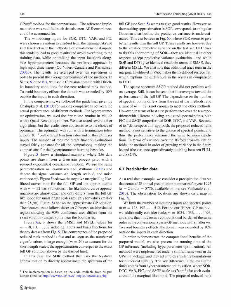
The m inducing inputs for SOR, DTC, VAR, and FICwere chosen at random as a subset from the training data andkept fixed between themethods. For low-dimensional inputs,this tends to lead to good results and avoid overfitting to thetraining data, while optimizing the input locations along-side hyperparameters becomes the preferred approach inhigh input dimensions (Quiñonero-Candela and Rasmussen2005b). The results are averaged over ten repetitions inorder to present the average performance of the methods. InSects. 6.2 and 6.3, we used a Cartesian domain with Dirich-let boundary conditions for the new reduced-rank method.To avoid boundary effects, the domain was extended by 10%outside the inputs in each direction.

In the comparisons, we followed the guidelines given byChalupka et al. (2013) for making comparisons between theactual performance of different methods. For hyperparame-ter optimization, we used the fminunc routine in Matlabwith a Quasi-Newton optimizer. We also tested several otheralgorithms, but the results were not sensitive to the choice ofoptimizer. The optimizer was run with a termination toler-ance of 10−5 on the target function value and on the optimizerinputs. The number of required target function evaluationsstayed fairly constant for all the comparisons, making thecomparisons for the hyperparameter learning bespoke.

Figure 5 shows a simulated example, where 256 datapoints are drawn from a Gaussian process prior with asquared exponential covariance function. We use the sameparametrization as Rasmussen and Williams (2006) anddenote the signal variance σ 2, length scale , and noisevariance σ 2

n . Figure 5b shows the negative marginal log like-lihood curves both for the full GP and the approximationwith m = 32 basis functions. The likelihood curve approx-imations are almost exact and only differs from the full GPlikelihood for small length scales (roughly for values smallerthan 2L/m). Figure 5a shows the approximate GP solution.Themean estimate follows the exactGPmean, and the shadedregion showing the 95% confidence area differs from theexact solution (dashed) only near the boundaries.

Figure 6a, b shows the SMSE and MSLL values form = 8, 10, . . . , 32 inducing inputs and basis functions forthe toy dataset from Fig. 5. The convergence of the proposedreduced rank method is fast and as soon as the number ofeigenfunctions is large enough (m = 20) to account for theshort length scales, the approximation converges to the exactfull GP solution (shown by the dashed line).

In this case, the SOR method that uses the Nyströmapproximation to directly approximate the spectrum of the

1 The implementation is based on the code available from MiguelLázaro-Gredilla: http://www.tsc.uc3m.es/~miguel/downloads.php.

full GP (see Sect. 5) seems to give good results. However, asthe resulting approximation in SOR corresponds to a singularGaussian distribution, the predictive variance is underesti-mated. This can be seen in Fig. 6b, where SOR seems to givebetter results than the full GP. These results are however dueto the smaller predictive variance on the test set. DTC triesto fix this shortcoming of SOR—they are identical in otherrespects except predictive variance evaluation—and whileSOR and DTC give identical results in terms of SMSE, theydiffer inMSLL.We also note that additional trace term in themarginal likelihood inVARmakes the likelihood surface flat,which explains the differences in the results in comparisonto DTC.

The sparse spectrum SSGP method did not perform wellon average. Still, it can be seen that it converges toward theperformance of the full GP. The dependence on the numberof spectral points differs from the rest of the methods, anda rank of m = 32 is not enough to meet the other methods.However, in terms of best case performance over the ten repe-titionswith different inducing inputs and spectral points, bothFIC and SSGP outperformed SOR, DTC, and VAR. Becauseof its “dense spectrum” approach, the proposed reduced-rankmethod is not sensitive to the choice of spectral points, andthus, the performance remained the same between repeti-tions. In terms of variance over the 10-fold cross-validationfolds, the methods in order of growing variance in the figurelegend (the variance approximately doubling between FULLand SSGP).

6.3 Precipitation data

As a real-data example, we consider a precipitation data setthat containUS annual precipitation summaries for year 1995(d = 2 and n = 5776, available online, see Vanhatalo et al.2013). The observation locations are shown on a map inFig. 7a.

We limit the number of inducing inputs and spectral pointsto m = 128, 192, . . . , 512. For the our Hilbert-GP method,we additionally consider ranks m = 1024, 1536, . . . , 4096,and show that this causes a computational burden of the sameorder as the conventional sparseGPmethodswith smallerms.To avoid boundary effects, the domain was extended by 10%outside the inputs in each direction.

In order to demonstrate the computational benefits of theproposed model, we also present the running time of theGP inference (including hyperparameter optimization). Allmethods were implemented under a similar framework in theGPstuff package, and they all employ similar reformulationsfor numerical stability. The key difference in the evaluationtimes comes from hyperparameter optimization, where SOR,DTC, VAR, FIC, and SSGP scale asO(nm2) for each evalu-ation of the marginal likelihood. The proposed reduced-rank

123

Statistics and Computing (2020) 30:419–446 435

(a) Observation locations

0 1500 3000mm

(b) The full GP (c) The reduced-rank method

Fig. 7 Interpolation of the yearly precipitation levels using reduced-rank GP regression. a The n = 5776 weather station locations. b, c The resultsfor the full GP model and the new reduced-rank GP method

method scales as O(m3) for each evaluation (after an initialcost of O(nm2)).

Figure 6c, d shows the SMSE and MSLL results for thisdata against evaluation time. On this scale, we note thatthe evaluation time and accuracy, both in terms of SMSEand MSLL, are alike for SOR, DTC, VAR, and FIC. SSGPis faster to evaluate in comparison with the Nyström fam-ily of methods, which comes from the simpler structureof the approximation. Still, the number of required spec-tral points to meet a certain average error level is larger forSSGP.

The results for the proposed reduced-rank method(Hilbert-GP) show that with two input dimensions, therequired number of basis functions is larger. For the firstseven points, we notice that even though the evaluation istwo orders of magnitude faster, the method performs onlyslightly worse in comparison with conventional sparse meth-ods. By considering higher ranks (the next seven points), ourmethod converges to the performance of the full GP (bothin SMSE and MSLL), while retaining a computational timecomparable to the conventional methods. This type of spatialmedium-size GP regression problems can thus be solved inseconds.

Figure 7b, c show interpolation of the precipitation lev-els using a full GP model and the reduced-rank method(m = 1728), respectively. The results are practically identi-cal, as is easy to confirm from the color surfaces. Obtainingthe reduced-rank result (including initialization and hyper-parameter learning) took slightly less than 30 s on a laptopcomputer (MacBook Air, Late 2010 model, 2.13 GHz, 4 GBRAM), while the full GP inference took approximately18 minutes.

6.4 Temperature data on the surface of the globe

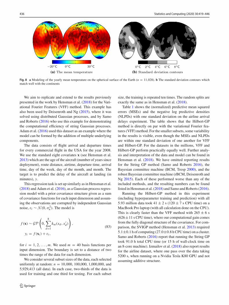
We also demonstrate the use of the method in non-Cartesiancoordinates. We consider modeling of the spatial mean tem-

perature over a number of n = 11,028 locations around theglobe.2

As earlier demonstrated in Fig. 2, we use the Laplaceoperator in spherical coordinates as defined in (31). Theeigenfunctions for the angular part are the Laplace’s spher-ical harmonics. The evaluation of the approximation doesnot depend on the coordinate system, and thus, all the equa-tions presented in the earlier sections remain valid. We usethe squared exponential covariance function and m = 1089basis functions.

Figure 8 visualizes the modeling outcome. The resultsare visualized using an interrupted projection (an adaptionof the Goode homolosine projection) in order to preservethe length-scale structure across the map. Fig. 8a shows theposterior mean temperature. The uncertainty is visualizedin Fig. 8b, which corresponds to the n = 11,028 obser-vation locations that are mostly spread over the continentsand Western countries (the white areas in Fig. 8b contain noobservations). Obtaining the reduced-rank result (includinginitialization and hyperparameter learning) took approxi-mately 50 s on a laptop computer (MacBook Air, Late 2010model, 2.13 GHz, 4 GB RAM), which scales with n in com-parison to the evaluation time in the previous section.

6.5 Additive modeling of airline delays

In order to fully use the computational benefits and alsounderline a way of applying the method to high-dimensionalinputs, we consider a large dataset for predicting airlinedelays. The US flight delay prediction example (originallyconsidered by Hensman et al. 2013) is a standard test data setinGaussian process regression. This is due to the clearly non-stationary behavior and itsmassive size, with nearly 6millionrecords.

2 The data are available for download from US National Cli-matic Data Center: http://www7.ncdc.noaa.gov/CDO/cdoselect.cmd(accessed January 3, 2014).

123

436 Statistics and Computing (2020) 30:419–446

−20◦C 0◦C 30◦C

(a) The mean temperature

0◦C 2◦C 4◦C 6◦C 8◦C

(b) Standard deviation contours

Fig. 8 a Modeling of the yearly mean temperature on the spherical surface of the Earth (n = 11,028). b The standard deviation contours whichmatch well with the continents

We aim to replicate and extend to the results previouslypresented in the work by Hensman et al. (2018) for the Vari-ational Fourier Features (VFF) method. This example hasalso been used by Deisenroth and Ng (2015), where it wassolved using distributed Gaussian processes, and by Samoand Roberts (2016) who use this example for demonstratingthe computational efficiency of string Gaussian processes.Adam et al. (2016) used this dataset as an example where themodel can be formed by the addition of multiple underlyingcomponents.

The data consists of flight arrival and departure timesfor every commercial flight in the USA for the year 2008.We use the standard eight covariates x (see Hensman et al.2013) which are the age of the aircraft (number of years sincedeployment), route distance, airtime, departure time, arrivaltime, day of the week, day of the month, and month. Thetarget is to predict the delay of the aircraft at landing (inminutes), y.

This regression task is set up similarly as inHensman et al.(2018) and Adam et al. (2016), as a Gaussian process regres-sion model with a prior covariance structure given as a sumof covariance functions for each input dimension and assum-ing the observations are corrupted by independent Gaussiannoise, εi ∼ N (0, σ 2

n ). The model is

f (x) ∼ GP(0,

8∑d=1

kse(xd , x ′d)

),

yi = f (xi ) + εi ,

(83)

for i = 1, 2, . . . , m. We used m = 40 basis functions perinput dimension. The boundary is set to a distance of twotimes the range of the data for each dimension.

We consider several subset sizes of the data, each selecteduniformly at random: n = 10,000, 100,000, 1,000,000, and5,929,413 (all data). In each case, two-thirds of the data isused for training and one third for testing. For each subset

size, the training is repeated ten times. The random splits areexactly the same as in Hensman et al. (2018).

Table 1 shows the (normalized) predictive mean squarederrors (MSEs) and the negative log predictive densities(NLPDs) with one standard deviation on the airline arrivaldelays experiment. The table shows that the Hilbert-GPmethod is directly on par with the variational Fourier fea-tures (VFF)method. For the smaller subsets, some variabilityin the results is visible, even though the MSEs and NLPDsare within one standard deviation of one another for VFFand Hilbert-GP. For the datasets in the millions, VFF andHilbert-GP perform practically equally well. Further analy-sis and interpretation of the data and model can be found inHensman et al. (2018). We have omitted reporting resultsfor the String GP method (Samo and Roberts 2016), theBayesian committee machine (BCM, Tresp 2000), and therobust Bayesian committee machine (rBCM, Deisenroth andNg 2015). Each of these performed worse than any of theincluded methods, and the resulting numbers can be foundlisted inHensman et al. (2018) and Samo andRoberts (2016).

Running the Hilbert-GP method in this experiment(including hyperparameter training and prediction) with all5.93 million data took 41 ± 2 s (120 ± 7 s CPU time) on aMacBook Pro laptop (with all calculation done on the CPU).This is clearly faster than the VFF method with 265 ± 6 s(626±11 s CPU time), where our computational gain comesfrom the fully diagonal structure of the covariance. For com-parison, the SVIGP method (Hensman et al. 2013) required5.1±0.1 h of computing (27.0±0.8 hCPU time) on a cluster.Samo and Roberts (2016) report that running the String GPtook 91.0 h total CPU time (or 15 h of wall-clock time onan 8-core machine). Izmailov et al. (2018) also report resultsfor the airline dataset, where one pass over the data taking5200 s, when running on a Nvidia Tesla K80 GPU and notassuming additive structure.

123

Statistics and Computing (2020) 30:419–446 437

Table 1 Predictive mean squared errors (MSEs) and negative log predictive densities (NLPDs) with one standard deviation on the airline arrivaldelays experiment (input dimensionality d = 8) for a number of data points ranging up to almost 6 million

n 10,000 100,000 1,000,000 5,929,413

MSE NLPD MSE NLPD MSE NLPD MSE NLPD

Hilbert-GP 0.97 ± 0.14 1.404 ± 0.071 0.80 ± 0.06 1.311 ± 0.038 0.83 ± 0.02 1.329 ± 0.011 0.827 ± 0.005 1.324 ± 0.003

VFF 0.89 ± 0.15 1.362 ± 0.091 0.82 ± 0.05 1.319 ± 0.030 0.83 ± 0.01 1.326 ± 0.008 0.827 ± 0.004 1.324 ± 0.003

SVIGP 0.89 ± 0.16 1.354 ± 0.096 0.79 ± 0.05 1.299 ± 0.033 0.79 ± 0.01 1.301 ± 0.009 0.791 ± 0.005 1.300 ± 0.003

Full-RBF 0.89 ± 0.16 1.349 ± 0.098 N/A N/A N/A N/A N/A N/A

Full-additive 0.89 ± 0.16 1.362 ± 0.096 N/A N/A N/A N/A N/A N/A

The Hilbert-GP method is on par with the VFFmethod albeit being clearly faster due to the diagonalizable structure (solving the regression problemincluding hyperparameter optimization in 41 s on a CPU-only laptop computer)

6.6 Gaussian process driven Poisson equation

Asdiscussed inSect. 3.4, our framework also directly extendsto inverse problems and latent force models. As this finalexperiment, we demonstrate the use of the approximation inthe latent force model (LFM)

−∇2g(x) = f (x),

yi = g(xi ) + εi ,(84)

where x ∈ R2 and f (x) ∼ GP(0, k(x, x′)) is the input with a

squared exponential covariance function prior. This problemcan also be interpreted as a inverse problem where the mea-surement operator is the Green’s operator H = (−∇2)−1:

yi = (H f )(xi ) + εi . (85)

If we assume that the boundary conditions of the problem arethe same as we used for forming the basis functions in (10),then if we put g(x) ≈ ∑m

j=1 g j φ j (x), we get

−∇2g(x) ≈ −m∑

j=1

g j ∇2φ j (x) =m∑

j=1

g j λ j φ j (x) (86)

and thus by further putting f (x) ≈ ∑mj=1 f j φ j (x), the

approximation to the equation −∇2g(x) = f (x) becomes

m∑j=1

g j λ j φ j (x) =m∑

j=1

f j φ j (x) (87)

which allows us to solve f j = g j/λ j . This implies that weapproximately have (−∇2)−1φ j = φ j/λ j which reducesEq. (52) to

(HH′ k)(x, x′) ≈∑

j

λ−2j S(

√λ j ) φ j (x) φ j (x′),

(H′k(x∗, ·))(x′) ≈∑

j

λ−1j S(

√λ j ) φ j (x∗) φ j (x′),

(88)

after which we can proceed with (51). Alternatively we candirectly use (53) with �̃i j = φ j (xi )/λ j .

Figure 9 shows the result of applying the proposedmethodto this model with the input function shown in Fig. 9b. Thetrue solution and the simulated measurements (with standarddeviation of 1/10) are shown in Fig. 9a. The scale σ 2 andlength scale of the SE covariance function were estimatedby maximum likelihood method, and the number of basisfunctions used for solving theGP regressionproblemwas100(for simulation we used 255 basis functions). The estimatesof the input and the solution function are shown in Fig. 9a, b,respectively. As can be seen in the figures, the estimate of thesolution is very good, as can be expected from the fact thatwe obtain direct (although noisy) measurements from it. Theestimate of the input is less accurate, but still approximatesthe true input well.

7 Conclusion and discussion

In this paper, we have proposed a novel approximationscheme for forming approximate eigendecompositions ofcovariance functions in terms of the Laplace operator eigen-basis and the spectral density of the covariance function. Theeigenfunction decomposition of the Laplacian can easily beformed in various domains, and the eigenfunctions are inde-pendent of the choice of hyperparameters of the covariance.

An advantage of the method is that it has the ability toapproximate the eigendecomposition using only the eigen-decomposition of the Laplacian and the spectral densityof the covariance function, both of which are closed-formexpressions. This together with having the eigenvectors in�

mutually orthogonal and independent of the hyperparame-ters, is the key to efficiency. This allows an implementationwith a computational cost of O(nm2) (initial) and O(m3)

(marginal likelihood evaluation), with negligible memoryrequirements.

Of the infinite number of possible basis functions, only anextremely small subset are of any relevance to the GP beingapproximated. InGP regression, themodel functions are con-ditioned on a covariance function (kernel), which imposes

123

438 Statistics and Computing (2020) 30:419–446

Fig. 9 Gaussian process inference on the Poisson equation

desired properties on the solutions.We choose the basis func-tions such that they are as close as possible (w.r.t. the Frobe-nius norm) to those of the particular covariance function. Ourmethod gives the exact eigendecomposition of a GP that hasbeen constrained to be zero at the boundary of the domain.

The method allows for theoretical analysis of the errorinduced by the truncation of the series and the boundaryeffects. This is something new in this context and extremelyimportant, for example, inmedical imaging applications. Theapproximative eigendecomposition also opens a range ofinteresting possibilities for further analysis. In learning curveestimation, the eigenvalues of the Gaussian process can nowbe directly approximated. For example, we can approximatethe Opper–Vivarelli bound (Opper and Vivarelli 1999) as

εOV(n) ≈ σ 2n

∑j

S(√

λ j )

σ 2n + n S(

√λ j )

. (89)

Sollich’s eigenvalue-based bounds (Sollich andHalees 2002)can be approximated and analyzed in an analogous way.

However, some of these abilities come with a cost. Asdemonstrated throughout the paper, restraining the domainto boundary conditions introduces edge effects. These are,however, known and can be accounted for. Extrapolatingwith a stationary covariance function outside the traininginputs only causes the predictions to revert to the prior meanand variance. Therefore, we consider the boundary effects aminor problem for practical use.

Although at first sight the method appears to have abad (exponential) scaling with respect to the input dimen-sionality, as shown by the analysis in Sect. 4.3, this isnot true. By increasing the differentiability order of thecovariance function appropriately we can keep the conver-gence rate at the level ∼1/ma , for a given constant a > 0and with total of m terms in the series, regardless of theinput dimensionality. Furthermore, Theorem 8 shows thatfor squared exponential covariance function the conver-gence rate is always better than ∼1/m, independently of theinput dimensionality. Further resources related to the pro-posed method and implementation details in form of code

123

Statistics and Computing (2020) 30:419–446 439

are available at https://urldefense.proofpoint.com/v2/url?u=https-3A__github.com_AaltoML_hilbert-2Dgp&d=DwIF-g&c=vh6FgFnduejNhPPD0fl_yRaSfZy8CWbWnIf4XJhSqx8&r=tr37p-LMKuZcfSC3Gl2yDumEEj4eKb1_KBfWD90OLbA&m=THRRZB0_Y9lwmhCaOrOo0bdjMjd0OsCoUzaXp0KoxtY&s=3V5psUm6EyKZqu53hd-Aij4hjaYtsPliYE1xSoBxYlQ&e=.

Acknowledgements Open access funding provided by Aalto Univer-sity. The authors would like to thank James Hensman and Manon Kokfor feedback on an early version of this paper,Mauricio Álvarez for helpin the latent forcemodel application as well as the referees for providingvaluable ideas for improving the article. This research was supported bythe Academy of Finland grants 308640 and 313708. We acknowledgethe computational resources provided by the Aalto Science-IT project.

Open Access This article is distributed under the terms of the CreativeCommons Attribution 4.0 International License (http://creativecommons.org/licenses/by/4.0/), which permits unrestricted use, distribution,and reproduction in any medium, provided you give appropriate creditto the original author(s) and the source, provide a link to the CreativeCommons license, and indicate if changes were made.

A Proofs of convergence theorems

A.1 Auxiliary lemmas

In this section,we present a few lemmas thatwill be needed inthe proofs in the next sections. The lemmas are quite classicalresults on the convergence of Riemannian sums, but as it ishard to find exactly the same results in other literature, forcompleteness we prove the lemmas here.

Lemma 9 Let � > 0 and α ∈ [0, 1) be given constants,m = 0, 1, 2, . . . some nonnegative integer and assumethat the f (ω) is a bounded integrable function defined onω ≥ m � with bounded derivative on ω > m � such that∫ ∞

m �| f ′(ω)| dω = C (m) < ∞. Then we have∣∣∣∣∣∣

∫ ∞

m �

f (ω) dω −∞∑

j=m+1

f ( j � − α �)�

∣∣∣∣∣∣ ≤ C (m) �. (90)

Furthermore, provided that∫ ∞0 | f ′(ω)| dω = C (0) < ∞,

this bound can be made independent of m:∣∣∣∣∣∣∫ ∞

m �

f (ω) dω −∞∑

j=m+1

f ( j � − α �)�

∣∣∣∣∣∣ ≤ C (0) �. (91)

Proof We can write∫ ∞

m �

f (ω) dω =∞∑

j=m+1

∫ j �

( j−1) �

f (ω) dω. (92)

By the fundamental theorem of calculus, we get

f (ω) = f ( j � − α �) +∫ ω

j �−α �

f ′(ω) dω, (93)

which gives for ω ∈ (( j − 1)�, j �]

| f (ω) − f ( j � − α �)| ≤∣∣∣∣∫ ω

j �−α �

f ′(ω) dω

∣∣∣∣≤

∣∣∣∣∫ ω

j �−α �

∣∣ f ′(ω)∣∣ dω

∣∣∣∣≤

∫ j �

( j−1) �

∣∣ f ′(ω)∣∣ dω

(94)

We now get

∣∣∣∣∣∣∫ ∞

m �

f (ω) dω −∞∑

j=m+1

f ( j � − α �)�

∣∣∣∣∣∣

=∣∣∣∣∣∣

∞∑j=m+1

∫ j �

( j−1) �

[ f (ω) − f ( j � − α �)] dω∣∣∣∣∣∣

≤∞∑

j=m+1

∫ j �

( j−1) �

| f (ω) − f ( j � − α �)| dω

≤∞∑

j=m+1

∫ j �

( j−1) �

[∫ j �

( j−1) �

∣∣ f ′(ω)∣∣ dω

]dω

=∞∑

j=m+1

∫ j �

( j−1) �

∣∣ f ′(ω)∣∣ dω �

=∫ ∞

m �

∣∣ f ′(ω)∣∣ dω

︸ ︷︷ ︸C(m)

� ≤∫ ∞

0

∣∣ f ′(ω)∣∣ dω

︸ ︷︷ ︸C(0)

�,

(95)

which concludes the proof. ��

Lemma 10 Assume that f (ω) is a bounded integrable func-tion defined on ω ≥ 0 with bounded derivative on ω > 0and g(ω) is a bounded function defined on ω ≥ 0 such that|g(w)| ≤ D. Further assume that

∫ ∞0 | f ′(ω)| dω = C < ∞.

Then for any α, β ∈ [0, 1) and � > 0 we have

∣∣∣∣∣∣∞∑j=1

[ f ( j �) − f ( j � − α �)] g( j � − β �)

∣∣∣∣∣∣ ≤ C D.

(96)

Proof By using (94) with ω = j � − α �, we get

| f ( j �) − f ( j � − α �)| ≤∫ j �

( j−1) �

∣∣ f ′(ω)∣∣ dω, (97)

123

440 Statistics and Computing (2020) 30:419–446

and further

∣∣∣∣∣∣∞∑j=1

[ f ( j �) − f ( j � − α �)] g( j � − β �)

∣∣∣∣∣∣≤

∞∑j=1

| f ( j �) − f ( j � − α �)| |g( j � − β �)|

≤∞∑j=1

∫ j �

( j−1) �

∣∣ f ′(ω)∣∣ dω D

=∫ ∞

0

∣∣ f ′(ω)∣∣ dω D

= C D.

(98)

��

Lemma 11 Assume that f (ω) ≥ 0 is a positive boundedintegrable function defined on ω ≥ 0 with bounded deriva-tive on ω > 0 such that

∫ ∞0 f (ω) dω = C0 < ∞ and∫ ∞

0 | f ′(ω)| dω = C1 ≤ ∞, and g(ω) is a bounded inte-grable function defined on ω ≥ 0 with bounded derivativeon ω > 0 such that |g′(ω)| ≤ D. Then for any α, β ∈ [0, 1)and � > 0 we have for C = C1 + C0:

∣∣∣∣∣∣∞∑j=1

f ( j � − α �) [g( j �) − g( j � − β �)]∣∣∣∣∣∣ ≤ C D.

(99)

Proof By applying the mean value theorem to (97), we getthat for some ω∗

j ∈ [ j � − α �, j �] we have

|g( j �) − g( j � − β �)|≤ |g′(ω∗

j )| β � ≤ |g′(ω∗j )| � ≤ D �.

(100)

By using Lemma 9, we get

∞∑j=1

f ( j � − α �)�

=∣∣∣∣∣∣

∞∑j=1

f ( j � − α �)� −∫ ∞

0f (ω) dω

+∫ ∞

0f (ω) dω

∣∣∣∣

≤∣∣∣∣∣∣

∞∑j=1

f ( j � − α �)� −∫ ∞

0f (ω) dω

∣∣∣∣∣∣+

∣∣∣∣∫ ∞

0f (ω) dω

∣∣∣∣≤ C1 + C0 = C .

(101)

Hence,

∣∣∣∣∣∣∞∑j=1

f ( j � − α �) [g( j �) − g( j � − β �)]∣∣∣∣∣∣

≤∞∑j=1

f ( j � − α �) |g( j �) − g( j � − β �)|

≤∞∑j=1

f ( j � − α �)� D

≤ C D.

(102)

��

A.2 Proof of Theorem 1

The Wiener–Khintchin identity and the symmetry of thespectral density allows us to write

k(x, x ′) = 1

2π

∫ ∞

−∞S(ω) exp(−iω (x − x ′)) dω

= 1

π

∫ ∞

0S(ω) cos(ω (x − x ′)) dω. (103)

In a one-dimensional domain Ω = [−L, L] with Dirichletboundary conditions, we have an m-term approximation ofthe form

k̃m(x, x ′) =m∑

j=1

S

(π j

2L

)1

Lsin

(π j (x + L)

2L

)

× sin

(π j (x ′ + L)

2L

).

(104)

We start by showing the convergence by growing the domainand therefore first consider an approximation with an infinitenumber of terms m = ∞:

k̃∞(x, x ′) =∞∑j=1

S

(π j

2L

)1

Lsin

(π j (x + L)

2L

)

× sin

(π j (x ′ + L)

2L

).

(105)

For that purpose, we rewrite the summation above in (105)as

∞∑j=1

S

(π j

2L

)1

Lsin

(π j (x + L)

2L

)sin

(π j (x ′ + L)

2L

)

=∞∑j=1

S

(π j

2L

)cos

(π j (x − x ′)

2L

)1

2L

− 1

2L

∞∑j=1

[S

(π 2 j

2L

)− S

(π (2 j − 1)

2L

)]

123

Statistics and Computing (2020) 30:419–446 441

× cos

(π 2 j (x + x ′)

2L

)

− 1

2L

∞∑j=1

S

(π (2 j − 1)

2L

) [cos

(π 2 j (x + x ′)

2L

)

− cos

(π (2 j − 1) (x + x ′)

2L

) ]. (106)

and consider the three summations above separately. Theanalysis of them is done in the next three lemmas.

Lemma 12 Assume that on ω ≥ 0 we have S(ω) ≤ B < ∞and

∫ ∞0 S(w) dω = A < ∞, and on ω > 0 S(ω)

has a bounded derivative |S′(ω)| ≤ D < ∞ and that∫ ∞0 |S′(ω)| dω = C < ∞. Then there exists a constant

D2 such that for all x, x ′ ∈ [−L̃, L̃] we have

∣∣∣∣∣∣∞∑j=1

S

(π j

2L

)cos

(π j (x − x ′)

2L

)1

2L

− 1

π

∫ ∞

0S(ω) cos(ω (x − x ′)) dω

∣∣∣∣ ≤ D2

L. (107)

Proof By using Lemma 9 with � = π2L , f (ω) = 1

πS(ω)

cos(ω (x − x ′)) dω, m = 0, and α = 0 as well as the assump-tions on S(ω) and boundedness of sine and cosine we get that

∣∣∣∣∣∣∞∑j=1

S

(π j

2L

)cos

(π j (x − x ′)

2L

)1

2L

− 1

π

∫ ∞

0S(ω) cos(ω (x − x ′)) dω

∣∣∣∣≤ 1

π

∫ ∣∣S′(w) cos(ω (x − x ′)) dω

− S(w) (x − x ′) sin(ω (x − x ′))∣∣ dω π

2L

≤ 1

2L

∫ ∣∣S′(w) cos(ω (x − x ′))∣∣ dω (108)

+ 1

2L

∫ ∣∣S(w) (x − x ′) sin(ω (x − x ′))∣∣ dω

≤ 1

2L

∫ ∣∣S′(w)∣∣ dω + |x − x ′|

2L

∫ ∣∣S(w)∣∣ dω

≤ 1

2L

∫ ∣∣S′(w)∣∣ dω + L̃

L

∫ ∣∣S(w)∣∣ dω

≤ 1

2LC + L̃

LA,

which gives the result with D2 = C2 + L̃ A. ��

Lemma 13 Assume that for ω ≥ 0, S(ω) is a bounded inte-grable function with a bounded derivative on ω > 0 suchthat

∫ ∞0 |S′(ω)| dω = C < ∞, then there exists a constant

D3 such that

∣∣∣∣∣∣1

2L

∞∑j=1

[S

(π 2 j

2L

)− S

(π (2 j − 1)

2L

)]

× cos

(π 2 j (x + x ′)

2L

)∣∣∣∣≤ D3

L.

(109)

Proof The result follows by using Lemma 10 with � = πL ,

α = 1/2, β = 0, f (ω) = S(ω), and g(ω) = cos(ω (x + x ′))and by recalling that | cos(ω (x + x ′))| ≤ 1, which gives theconstant D3 = C

2 . ��Lemma 14 Assume that for ω ≥ 0, S(ω) is a bounded pos-itive integrable function with bounded derivative on ω > 0such that

∫ ∞0 S(ω) dω = A < ∞ and

∫ ∞0 |S′(ω)| dω =

C < ∞. Then there exists a constant D4 such that∣∣∣∣∣∣1

2L

∞∑j=1

S

(π (2 j − 1)

2L

) [cos

(π 2 j (x + x ′)

2L

)

− cos

(π (2 j − 1) (x + x ′)

2L

)∣∣∣∣ ≤ D4

L.

Proof By using Lemma 11 with � = πL , α = 1/2, β = 1/2,

f (ω) = S(ω), and g(ω) = cos(ω (x + x ′)) we get∣∣∣∣∣∣1

2L

∞∑j=1

S

(π (2 j − 1)

2L

) [cos

(π 2 j (x + x ′)

2L

)

− cos

(π (2 j − 1) (x + x ′)

2L

)∣∣∣∣≤ (A + C) D′

2L,

where D′ is an upper bound for |(x + x ′) sin(ω (x + x ′))|.We can now select D′ = 2L̃ , which gives D4 = (A + C)

L̃ . ��Next, we combine the above lemmas to get the following

result.

Lemma 15 Let the assumptions of Lemmas 12, 13, and 14be satisfied. Then there exists a constant D1 such that for allx, x ′ ∈ [− L̃, L̃] we have

∣∣∣∣∣∣∞∑j=1

S

(π j

2L

)1

Lsin

(π j (x + L)

2L

)× sin

(π j (x ′ + L)

2L

)

− 1

π

∫ ∞

0S(ω) cos(ω (x − x ′)) dω

∣∣∣∣ ≤ D1

L. (110)

That is,

∣∣̃k∞(x, x ′) − k(x, x ′)∣∣ ≤ D1

L, for x, x ′ ∈ [−L̃, L̃]. (111)

123

442 Statistics and Computing (2020) 30:419–446

Furthermore, the explicit expression for the constant is givenas

D1 = C + (2A + C) L̃. (112)

Proof Using triangle inequality to the difference of (106) and1π

∫ ∞0 S(ω) cos(ω (x − x ′)) dω along with Lemmas 12, 13,

and 14 gives

∣∣∣∣∣∣∞∑j=1

S

(π j

2L

)cos

(π j (x − x ′)

2L

)1

2L

− 1

2L

∞∑j=1

[S

(π 2 j

2L

)− S

(π (2 j − 1)

2L

)]

× cos

(π 2 j (x + x ′)

2L

)

− 1

2L

∞∑j=1

S

(π (2 j − 1)

2L

) [cos

(π 2 j (x + x ′)

2L

)

− cos

(π (2 j − 1) (x + x ′)

2L

)]

− 1

π

∫ ∞

0S(ω) cos(ω (x − x ′)) dω

∣∣∣∣

≤∣∣∣∣∣∣

∞∑j=1

S

(π j

2L

)cos

(π j (x − x ′)

2L

)1

2L

− 1

π

∫ ∞

0S(ω) cos(ω (x − x ′)) dω

∣∣∣∣

+∣∣∣∣ 1

2L

∞∑j=1

[S

(π 2 j

2L

)− S

(π (2 j − 1)

2L

)]

× cos

(π 2 j (x + x ′)

2L

)∣∣∣∣

+∣∣∣∣∣∣1

2L

∞∑j=1

S

(π (2 j − 1)

2L

) [cos

(π 2 j (x + x ′)

2L

)

− cos

(π (2 j − 1) (x + x ′)

2L

) ]∣∣∣∣≤ D2

L+ D3

L+ D4

L= D1

L, (113)

where the explicit values for the constants can be found inthe proofs of the lemmas. ��

Let us now consider what happens when we replace theinfinite sum approximation with a finite m number of terms.We are now interested in

k̃∞(x, x ′) − k̃m(x, x ′)

=∞∑

j=m+1

S

(π j

2L

)1

Lsin

(π j (x + L)

2L

)

× sin

(π j (x ′ + L)

2L

).

(114)

Lemma 16 Assume that on ω ≥ 0, S(ω) is bounded andintegrable, on ω > 0 it has a bounded derivative, and that∫ ∞0 |S′(ω)| dω = C < ∞. Then there exists a constant D5

such that for all x, x ′ ∈ [−L̃, L̃] we have

∣∣̃k∞(x, x ′) − k̃m(x, x ′)∣∣ ≤ D5

L+ 2

π

∫ ∞π m2L

S(ω) dω. (115)

Proof Because the sinusoidals are bounded by unity, we get∣∣∣∣∣∣∞∑

j=m+1

S

(π j

2L

)1

Lsin

(π j (x + L)

2L

)

× sin

(π j (x ′ + L)

2L

)∣∣∣∣

≤∣∣∣∣∣∣

∞∑j=m+1

S

(π j

2L

)1

L

∣∣∣∣∣∣ . (116)

For the right-hand side, we can now use Lemma 9 withf (ω) = 2

πS(ω) and � = π

2L , which gives∣∣∣∣∣∣

∞∑j=m+1

S

(π j

2L

)1

L− 2

π

∫ ∞π m2L

S(ω) dω

∣∣∣∣∣∣ ≤ Cπ

2L= D5

L.

(117)

Hence by the triangle inequality we get∣∣∣∣∣∣∞∑

j=m+1

S

(π j

2L

)1

L

∣∣∣∣∣∣

=∣∣∣∣∣∣

∞∑j=m+1

S

(π j

2L

)1

L− 2

π

∫ ∞π m2L

S(ω) dω

+ 2

π

∫ ∞π m2L

S(ω) dω

∣∣∣∣∣

≤∣∣∣∣∣∣

∞∑j=m+1

S

(π j

2L

)1

L− 2

π

∫ ∞π m2L

S(ω) dω

∣∣∣∣∣∣+ 2

π

∫ ∞π m2L

S(ω) dω

≤ D5

L+ 2

π

∫ ∞π m2L

S(ω) dω (118)

and thus the result follows. ��

123

Statistics and Computing (2020) 30:419–446 443

Remark 17 We can also obtain a bit more defined bound bynot using an m-independent bound for forming D5, whichunder the assumptions of Lemma 16 gives

∣∣̃k∞(x, x ′) − k̃m(x, x ′)∣∣

≤ π

2L

∫ ∞π m2L

|S′(ω)| dω + 2

π

∫ ∞π m2L

S(ω) dω.(119)

The lemmas presented in this section can now be com-bined to a proof of the one-dimensional convergence theoremas follows:

Proof of Theorem 1 The first result follows by combiningLemmas 15 and 16 via the triangle inequality. Because ourassumptions imply that

limx→∞

∫ ∞

xS(ω) dω = 0, (120)

for any fixed L we have

limm→∞

[E

L+ 2

π

∫ ∞π m2L

S(ω) dω

]→ E

L. (121)

If we now take the limit L → ∞, the second result in thetheorem follows. ��

A.3 Proof of Theorem 4

When x ∈ Rd , the Wiener–Khintchin identity and symmetry

of the spectral density imply that

k(x, x′) = 1

(2π)d

∫Rd

S(ω) exp(−iωT(x − x′)) dω

= 1

πd

∫ ∞

0· · ·

∫ ∞

0S(ω)

d∏k=1

cos(ωk (xk − x ′k)) dω1 · · · dωd .

(122)

The m = m̂d term approximation now has the form

k̃m(x, x′) =m̂∑

j1,..., jd=1

S

(π j12L1

, . . . ,π jd2Ld

)

×d∏

k=1

1

Lksin

(π jk (xk + Lk)

2Lk

)

× sin

(π jk (x ′

k + Lk)

2Lk

). (123)

As in the one-dimensional problem, we start by consider-ing the case where m̂ = ∞.

Lemma 18 Let the assumptions of Lemma 15 be satisfied foreach ω j �→ S(ω1, . . . , ωd) separately. Then there exists aconstant D1 such that for all x, x′ ∈ [−L̃, L̃]d we have∣∣∣∣∣∣

∞∑j1,..., jd =1

S

(π j12L1

, . . . ,π jd2Ld

)×

d∏k=1

1

Lksin

(π jk (xk + Lk)

2Lk

)

× sin

(π jk (x ′

k + Lk)

2Lk

)

− 1

πd

∫ ∞

0· · ·

∫ ∞

0S(ω)

d∏k=1

cos(ωk (x − x ′)) dω1 · · · dωd

∣∣∣∣∣

≤ D1

d∑k=1

1

Lk≤ D1 d

L, (124)

where L = mink Lk. That is, for all x, x′ ∈ [−L̃, L̃]d

∣∣̃k∞(x, x′) − k(x, x′)∣∣ ≤ D1

d∑k=1

1

Lk≤ D1 d

L. (125)

Proof We can separate the summation over j1 as follows:

∞∑j2,..., jd=1

⎡⎣ ∞∑

j1=1

S

(π j12L1

, . . . ,π jd2Ld

)1

L1

× sin

(π j1 (x1 + L1)

2L1

)sin

(π j1 (x ′

1 + L1)

2L1

)]

×d∏

k=2

1

Lksin

(π jk (xk + Lk)

2Lk

)

× sin

(π jk (x ′

k + Lk)

2Lk

). (126)

By Lemma 15, there now exists a constant D1,1 such that∣∣∣∣∣∣

∞∑j1=1

S

(π j12L1

, . . . ,π jd2Ld

)1

L1

× sin

(π j1 (x1 + L1)

2L1

)sin

(π j1 (x ′

1 + L1)

2L1

)

− 1

π

∫ ∞

0S

(ω1,

π j22L2

, . . . ,π jd2Ld

)

× cos(ω1 (x1 − x ′1)) dω1

∣∣≤ D1,1

L1. (127)

The triangle inequality then gives

∣∣∣∣∣∣∞∑

j1,..., jd =1

S

(π j12L1

, . . . ,π jd2Ld

)×

d∏k=1

1

Lksin

(π jk (xk + Lk)

2Lk

)

× sin

(π jk (x ′

k + Lk)

2Lk

)

123

444 Statistics and Computing (2020) 30:419–446

− 1

πd

∫ ∞

0· · ·

∫ ∞

0S(ω)

d∏k=1

cos(ω j (xk − x ′k)) dω1 · · · dωd

∣∣∣∣∣

≤ D1,1

L1+

∣∣∣∣∣∣1

π

∞∑j2,..., jd =1

∫ ∞

0S

(ω1,

π j22L2

, . . . ,π jd2Ld

)

× cos(ω1 (x1 − x ′1)) dω1

×d∏

k=2

1

Lksin

(π jk (xk + Lk)

2Lk

)sin

(π jk (x ′

k + Lk)

2Lk

)

− 1

πd

∫ ∞

0· · ·

∫ ∞

0S(ω)

d∏k=1

cos(ωk (xk − x ′k)) dω1 · · · dωd

∣∣∣∣∣ .(128)

We can now similarly bound with respect to the summationsover j2, . . . , jd which leads to a bound of the form D1,1

L1+

· · · + D1,dLd

. Taking D1 = maxk D1,k leads to the desiredresult. ��

Nowwe can consider what happens in the finite truncationof the series. That is, we analyze the following residual sum

k̃∞(x, x′) − k̃m(x, x′)

=∞∑

j1,..., jd=m̂+1

S

(π j12L1

, . . . ,π jd2Ld

)

×d∏

k=1

1

Lksin

(π jk (xk + Lk)

2Lk

)

× sin

(π jk (x ′

k + Lk)

2Lk

). (129)

Lemma 19 Let assumptions of Lemma 16 be satisfied foreach ω j �→ S(ω1, . . . , ωd). There exists a constant D2 suchthat for all x, x′ ∈ [−L̃, L̃]d we have

∣∣̃k∞(x, x′) − k̃m(x, x′)∣∣ ≤ D2 d

L+ 1

πd

∫‖ω‖≥ π m̂

2L

S(ω) dω,

(130)

where L = mink Lk.

Proof We can write the following bound

∣∣∣∣∞∑

j1,..., jd=m̂+1

S

(π j12L1

, . . . ,π jd2Ld

)

×d∏

k=1

1

Lksin

(π jk (xk + Lk)

2Lk

)

× sin

(π jk (x ′

k + Lk)

2Lk

) ∣∣∣∣

≤∣∣∣∣

∞∑j1,..., jd=m̂+1

S

(π j12L1

, . . . ,π jd2Ld

) d∏k=1

1

Lk

∣∣∣∣. (131)

We can nowuseLemma9with f (ω1) = 2π

S(ω1,

π j22L2

, . . . ,

π jd2Ld

)and � = π

2L1, which gives

∣∣∣∣∣∣∞∑

j1,..., jd=m̂+1

S

(π j12L1

, . . . ,π jd2Ld

) d∏k=1

1

Lk

− 2

π

∞∑j2,..., jd=m̂+1

×∫ ∞

π m̂2L1

S

(ω1,

π j22L2

, . . . ,π jd2Ld

)dω1

d∏k=2

1

Lk

∣∣∣∣∣≤ D2,1

L1. (132)

Using a similar argument again, we get

∣∣∣∣∣∣2

π

∞∑j2,..., jd=m̂+1

∫ ∞π m̂2L1

S

(ω1,

π j22L2

, . . . ,π jd2Ld

)dω1

d∏k=2

1

Lk

− 22

π2

∞∑j3,..., jd=m̂+1

∫ ∞π m̂2L1

×∫ ∞

π m̂2L2

S

(ω1, ω2,

π j32L3

, . . . ,π jd2Ld

)dω1 dω2

×d∏

k=3

1

Lk

∣∣∣∣∣ ≤ D2,2

L2. (133)

After repeating this for all the indexes, by forming a telescop-ing sum of the terms and applying the triangle inequality thengives

∣∣∣∣∣∣∞∑

j1,..., jd=m̂+1

S

(π j12L1

, . . . ,π jd2Ld

) d∏k=1

1

Lk

−(2

π

)d ∫ ∞π m̂2L1

· · ·∫ ∞

π m̂2Ld

S(ω1, . . . , ωd) dω1 · · · dωd

∣∣∣∣∣

≤d∑

k=1

D2,k

Lk. (134)

123

Statistics and Computing (2020) 30:419–446 445

Applying the triangle inequality again gives

∣∣∣∣∣∣∞∑

j1,..., jd=m̂+1

S

(π j12L1

, . . . ,π jd2Ld

) d∏k=1

1

Lk

∣∣∣∣∣∣

≤d∑

k=1

D2,k

Lk+

(2

π

)d ∫ ∞π m̂2L1

· · ·∫ ∞

π m̂2Ld

S(ω1, . . . , ωd) dω1 · · · dωd . (135)

By interpreting the latter integral as being over the positiveexterior of a rectangular hypercuboid and bounding it by aintegral over exterior of a hypersphere which fits inside thecuboid, we can bound the expression by

d∑k=1

D2,k

Lk+ 1

πd

∫‖ω‖≥ π m̂

2L

S(ω) dω. (136)

The first term can be further bounded by replacing Lks withtheir minimum L and by defining D2 = max D2,k which isd times the maximum of D2,k . This leads to the final form ofthe result. ��Remark 20 Note that analogous to Remark 17 we couldtighten the bound for D2 by letting it depend on m̂.

Proof of Theorem 4 Analogous to the one-dimensional case,we combine the results of the above lemmas using the triangleinequality. ��

References

Adam, V., Hensman, J., Sahani, M.: Scalable transformed additive sig-nal decomposition by non-conjugate Gaussian process inference.In: IEEE International Workshop on Machine Learning for SignalProcessing (MLSP) (2016)

Adler, R.J.: The Geometry of Random Fields, vol. 62. SIAM, Philadel-phia (1981)

Akhiezer, N.I., Glazman, I.M.: Theory of Linear Operators in HilbertSpace. Dover, New York (1993)

Álvarez, M.A., Luengo, D., Lawrence, N.D.: Linear latent force modelsusing Gaussian processes. IEEE Trans. Pattern Anal. Mach. Intell.35(11), 2693–2705 (2013)

Bach, F.: Sharp analysis of low-rank kernel matrix approximations. In:Proceedings of the 26th Annual Conference on Learning Theory(COLT), PMLR, Princeton, NJ, USA, Proceedings of MachineLearning Research, vol. 30, pp. 185–209 (2013)

Baker, C.T.H.: The Numerical Treatment of Integral Equations. Claren-don Press, Oxford (1977)

Boutsidis, C., Gittens, A.: Improved matrix algorithms via the sub-sampled randomized Hadamard transform. SIAM J. Matrix Anal.Appl. 34(3), 1301–1340 (2013)

Brooks, S., Gelman, A., Jones, G.L., Meng, X.L.: Handbook ofMarkovChain Monte Carlo. Chapman & Hall, London (2011)

Bui, T.D., Yan, J., Turner, R.E.: A unifying framework for Gaussianprocess pseudo-point approximations using power expectationpropagation. J. Mach. Learn. Res. 18(104), 1–72 (2017)

Chalupka, K., Williams, C.K.I., Murray, I.: A framework for evaluatingapproximation methods for Gaussian process regression. J. Mach.Learn. Res. 14, 333–350 (2013)

Courant, R., Hilbert, D.: Methods of Mathematical Physics, vol. 1.Wiley, Hoboken (2008)

Cramér, H., Leadbetter, M.R.: Stationary and Related Stochastic Pro-cesses: Sample FunctionProperties andTheirApplications.Dover,Mineola (2013)

Csató, L., Opper, M.: Sparse online Gaussian processes. Neural Com-put. 14(3), 641–668 (2002)

Da Prato, G., Zabczyk, J.: Stochastic Equations in Infinite Dimensions,Encyclopedia of Mathematics and Its Applications, vol. 45. Cam-bridge University Press, Cambridge (1992)

Deisenroth,M.P., Ng, J.W.: DistributedGaussian processes. In: Interna-tional Conference on Machine Learning (ICML), pp. 1481–1490(2015)

Duane, S., Kennedy, A.D., Pendleton, B.J., Roweth, D.: Hybrid MonteCarlo. Phys. Lett. B 195(2), 216–222 (1987)

Feller, W.: An Introduction to Probability Theory and Its Applications,vol. I, 3rd edn. Wiley, Hoboken (1968)

Fritz, J.,Neuweiler, I.,Nowak,W.:Application of FFT-based algorithmsfor large-scale universal Kriging problems. Math. Geosci. 41(5),509–533 (2009)

Gal, Y., Turner, R.: Improving the Gaussian process sparse spectrumapproximation by representing uncertainty in frequency inputs.In: Proceedings of the 32nd International Conference on MachineLearning, Proceedings ofMachine Learning Research, vol. 37, pp.655–664 (2015)

Gardner, J., Pleiss, G.,Wu, R.,Weinberger, K.,Wilson, A.: Product ker-nel interpolation for scalable Gaussian processes. In: Proceedingsof the 21st International Conference on Artificial Intelligence andStatistics (AISTATS), Proceedings ofMachineLearningResearch,PMLR, Playa Blanca, Lanzarote, Canary Islands, vol. 84, pp.1407–1416 (2018)

Golub, G.H., Van Loan, C.F.: Matrix Computations, 3rd edn. JohnsHopkins University Press, Baltimore (1996)

Harbrecht, H., Peters, M., Schneider, R.: On the low-rank approxima-tion by the pivoted Cholesky decomposition. Appl. Numer. Math.4(62), 428–440 (2012)

Hensman, J., Fusi, N., Lawrence, N.D.: Gaussian processes for big data.In: Proceedings of the 29th Conference onUncertainty in ArtificialIntelligence (UAI 2013), pp. 282–290 (2013)

Hensman, J., Durrande, N., Solin, A.: Variational Fourier features forGaussian processes. J. Mach. Learn. Res. 8(151), 1–52 (2018)

Izmailov, P., Novikov, A., Kropotov, D.: Scalable Gaussian processeswith billions of inducing inputs via tensor train decomposition.In: Proceedings of the 21st International Conference on ArtificialIntelligence andStatistics (ICML), Proceedings ofMachineLearn-ing Research, PMLR, Playa Blanca, Lanzarote, Canary Islands,vol. 84, pp. 726–735 (2018)

Kaipio, J., Somersalo, E.: Statistical and Computational Inverse Prob-lems. Springer, Berlin (2005)

Kimeldorf, G.S., Wahba, G.: A correspondence between Bayesian esti-mation on stochastic processes and smoothing by splines. Ann.Math. Stat. 41, 495–502 (1970)

Lázaro-Gredilla,M.: SparseGaussian processes for large-scalemachinelearning. Ph.D. Thesis, Universidad Carlos III de Madrid, Madrid,Spain (2010)

Lázaro-Gredilla, M., Quiñonero-Candela, J., Rasmussen, C.E.,Figueiras-Vidal, A.R.: Sparse spectrum Gaussian process regres-sion. J. Mach. Learn. Res. 11, 1865–1881 (2010)

Le, Q., Sarlos, T., Smola, A.: Fastfood—computing Hilbert spaceexpansions in loglinear time. In: Proceedings of the 30th Interna-tional Conference on Machine Learning (ICML), PMLR, Atlanta,Georgia, USA, Proceedings of Machine Learning Research,vol. 28, pp. 244–252 (2013)

123

446 Statistics and Computing (2020) 30:419–446

Lenk, P.J.: Towards a practicable Bayesian nonparametric density esti-mator. Biometrika 78(3), 531–543 (1991)

Lindgren, F., Rue, H., Lindström, J.: An explicit link between Gaus-sian fields and Gaussian Markov random fields: the stochasticpartial differential equation approach. J. R. Stat. Soc. Ser. B (Stat.Methodol.) 73(4), 423–498 (2011)

Liu, J.S.: Monte Carlo Strategies in Scientific Computing. Springer,New York (2001)

Loève, M.: Probability Theory. The University Series in Higher Math-ematics, 3rd edn. Van Nostrand, Princeton (1963)

Neal, R.M.: MCMC using Hamiltonian dynamics. In: Brooks, S., Gel-man, A., Jones, G.L., Meng, X.L. (eds.) Handbook of MarkovChain Monte Carlo, Chap 5. Chapman & Hall, London (2011)

Opper, M., Vivarelli, F.: General bounds on Bayes errors for regressionwith Gaussian processes. Adv. Neural Inf. Process. Syst. 11, 302–308 (1999)

Paciorek, C.J.: Bayesian smoothing with Gaussian processes usingFourier basis functions in the spectralGP package. J. Stat. Softw.19(2), 1–38 (2007)

Quiñonero-Candela, J., Rasmussen, C.E.: Analysis of some methodsfor reduced rank Gaussian process regression. In: Switching andLearning in Feedback Systems, Lecture Notes in Computer Sci-ence, vol. 3355, pp. 98–127. Springer (2005)

Quiñonero-Candela, J., Rasmussen, C.E.: A unifying view of sparseapproximate Gaussian process regression. J. Mach. Learn. Res. 6,1939–1959 (2005)

Rasmussen, C.E., Williams, C.K.I.: Gaussian Processes for MachineLearning. The MIT Press, Cambridge (2006)

Saatçi, Y.: Scalable inference for structured Gaussian process models.Ph.D. Thesis, University of Cambridge, UK (2012)

Samo, Y.L.K., Roberts, S.J.: String and membrane Gaussian processes.J. Mach. Learn. Res. 17, 1–87 (2016)

Särkkä, S.: Linear operators and stochastic partial differential equationsin Gaussian process regression. In: Proceedings of ICANN (2011)

Särkkä, S., Hartikainen, J.: Infinite-dimensional Kalman filteringapproach to spatio-temporal Gaussian process regression. In:Proceedings of the 15th International Conference on ArtificialIntelligence and Statistics (AISTATS), JMLRWorkshop and Con-ference Proceedings, vol. 22, pp. 993–1001 (2012)

Särkkä, S., Piché, R.: On convergence and accuracy of state-spaceapproximations of squared exponential covariance functions. In:Proceedings of MLSP, pp. 1–6 (2014)

Särkkä, S., Solin, A., Hartikainen, J.: Spatiotemporal learning viainfinite-dimensional Bayesian filtering and smoothing. IEEE Sig-nal Process. Mag. 30(4), 51–61 (2013)

Seeger, M., Williams, C.K.I., Lawrence, N.D.: Fast forward selectionto speed up sparse Gaussian process regression. In: Proceedingsof the 9th International Workshop on Artificial Intelligence andStatistics (AISTATS) (2003)

Showalter, R.E.: Hilbert Space Methods in Partial Differential Equa-tions. Dover Publications, Mineola (2010)

Shubin, M.A.: Pseudodifferential Operators and Spectral Theory.Springer Series in Soviet Mathematics. Springer, Berlin (1987)

Smola, A.J., Bartlett, P.: Sparse greedy Gaussian process regression.In: Advances in Neural Information Processing Systems, vol. 13(2001)

Snelson, E., Ghahramani, Z.: Sparse Gaussian processes using pseudo-inputs. Adv. Neural Inf. Process. Syst. 18, 1259–1266 (2006)

Sollich, P., Halees, A.: Learning curves forGaussian process regression:approximations and bounds. Neural Comput. 14(6), 1393–1428(2002)

Tarantola, A.: Inverse Problem Theory and Methods for Model Param-eter Estimation. SIAM, Philadelphia (2004)

Titsias, M.K.: Variational learning of inducing variables in sparseGaussian processes. In: Proceedings of the 12th International Con-ference on Artificial Intelligence and Statistics (AISTATS), JMLRWorkshop andConferenceProceedings, vol. 5, pp. 567–574 (2009)

Tresp, V.: A Bayesian committee machine. Neural Comput. 12(11),2719–2741 (2000)

Van Trees, H.L.: Detection, Estimation, and Modulation Theory Part I.Wiley, New York (1968)

Vanhatalo, J., Pietiläinen,V.,Vehtari,A.:Approximate inference for dis-ease mapping with sparse Gaussian processes. Stat. Med. 29(15),1580–1607 (2010)

Vanhatalo, J., Riihimäki, J., Hartikainen, J., Jylänki, P., Tolvanen, V.,Vehtari, A.: GPstuff: Bayesian modeling with Gaussian processes.J. Mach. Learn. Res. 14, 1175–1179 (2013)

Wahba,G.: Improper priors, spline smoothing and the problemof guard-ing against model errors in regression. J. R. Stat. Soc. Ser. B(Methodol.) 40, 364–372 (1978)

Wahba, G.: Spline Models for Observational Data. SIAM, Philadelphia(1990)

Williams, C.K.I., Seeger,M.: The effect of the input density distributionon kernel-based classifiers. In: Proceedings of the 17th Interna-tional Conference on Machine Learning (2000)

Williams, C.K.I., Seeger, M.: Using the Nyström method to speed upkernel machines. In: Advances in Neural Information ProcessingSystems, vol. 13 (2001)

Wilson, A., Nickisch, H.: Kernel interpolation for scalable structuredGaussian processes (KISS-GP). In: Proceedings of the 32nd Inter-national Conference on Machine Learning (ICML), Proceedingsof Machine Learning Research, PMLR, Lille, France, vol. 37, pp.1775–1784 (2015)

Publisher’s Note Springer Nature remains neutral with regard to juris-dictional claims in published maps and institutional affiliations.

123