Embed Size (px)
Citation preview

Numerical Methods for Partial Differential Equations
CAAM 452Spring 2005
Lecture 41-step time-stepping methods: stability, accuracy
Runge-Kutta Methods,Instructor: Tim Warburton
CAAM 452 Spring 2005
Today
• Recall AB stability regions and start up issues• Group analysis of the Leap-Frog scheme
• One-step methods• Example Runge-Kutta methods:
– Modified Euler– General family of 2nd order RK methods– Heun’s 3rd Order Method– The 4th Order “Runge-Kutta” method– Jameson-Schmidt-Turkel
• Linear Absolute Stability Regions for the 2nd order family RK• Global error analysis for general 1-step methods (stops slightly short of
a full convergence analysis)• Warning on usefulness of global error estimate• Discussion on AB v. RK• Embedded lower order RK schemes useful for a posteriori error
estimates.
CAAM 452 Spring 2005
Recall: AB2 v. AB3 v. AB4
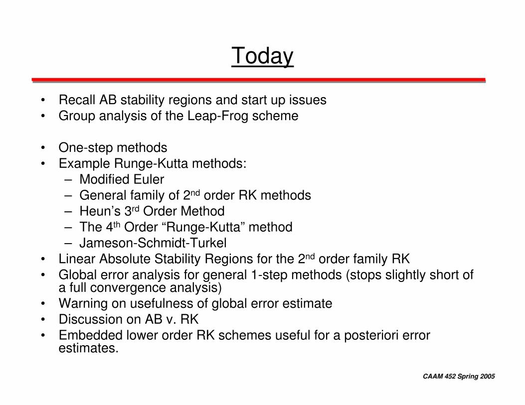
• These are the margins of absolute stability for the AB methods:
• Starting with the yellow AB1 (Euler-Forward) we see that as the order of accuracy goes up the stability region shrinks.
• i.e. we see that to use the higher order accurate AB scheme we are required to take more time steps.
Q) how many more?
CAAM 452 Spring 2005
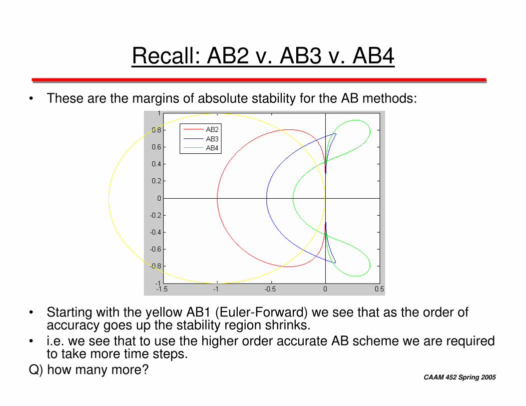
Recall:Requirements Starting Requirements
AB1:
AB2:
AB3:
( )( )
( ) ( )
1
0
1 1
0
3 12 2n n n n
u u dt
u u
u u dt f u f u
−
+ −
= −=
� �= + −� �� �
( )( )( )
0
1
0
n n n
u u
u u dt f u+
=
= +
( )( )
( )
( )
2
1
0
1 1 2
2
0
23 16 512n n n n n
u u dt
u u dt
u u
dtu u f f f
−
−
+ − −
= −= −
=
= + − +
1 solution level for start
2 solution levels for start
3 solution levels for start
CAAM 452 Spring 2005
cont
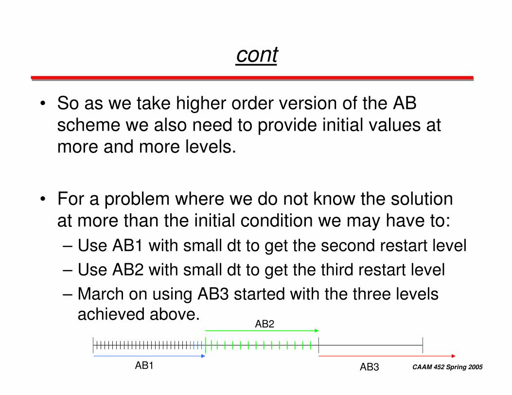
• So as we take higher order version of the AB scheme we also need to provide initial values at more and more levels.
• For a problem where we do not know the solution at more than the initial condition we may have to:– Use AB1 with small dt to get the second restart level– Use AB2 with small dt to get the third restart level– March on using AB3 started with the three levels
achieved above.
AB1
AB2
AB3
CAAM 452 Spring 2005
Recall: Derivation of AB Schemes
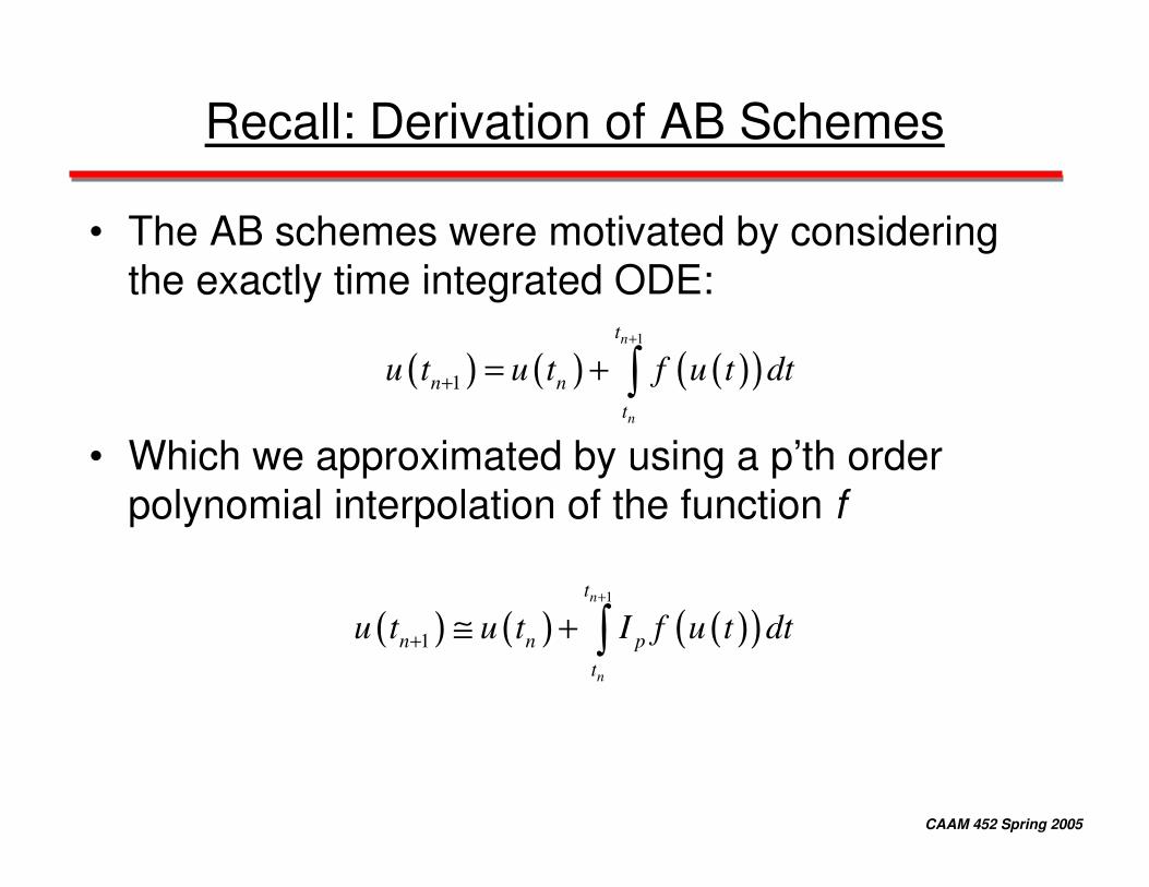
• The AB schemes were motivated by considering the exactly time integrated ODE:
• Which we approximated by using a p’th order polynomial interpolation of the function f
( ) ( ) ( )( )1
1
n
n
t
n nt
u t u t f u t dt+
+ = + �
( ) ( ) ( )( )1
1
n
n
t
n n pt
u t u t I f u t dt+
+ ≅ + �
CAAM 452 Spring 2005
Leap Frog Scheme
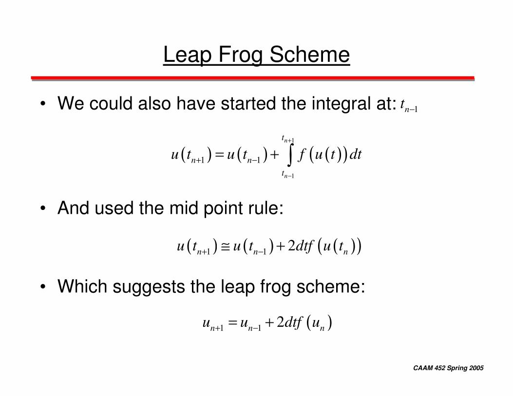
• We could also have started the integral at:
• And used the mid point rule:
• Which suggests the leap frog scheme:
1nt −
( ) ( ) ( )( )1
1
1 1
n
n
t
n nt
u t u t f u t dt+
−
+ −= + �
( ) ( ) ( )( )1 1 2n n nu t u t dtf u t+ −≅ +
( )1 1 2n n nu u dtf u+ −= +
CAAM 452 Spring 2005
Volunteer Exercise
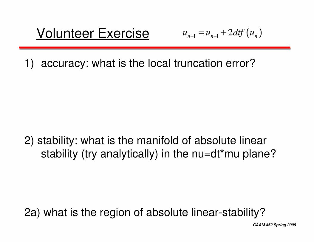
1) accuracy: what is the local truncation error?
2) stability: what is the manifold of absolute linear stability (try analytically) in the nu=dt*mu plane?
2a) what is the region of absolute linear-stability?
( )1 1 2n n nu u dtf u+ −= +
CAAM 452 Spring 2005
cont
3) How many starting values are required?
4) Do we have convergence?
5) What is the global order of accuracy?
6) When is this a good method?
( )1 1 2n n nu u dtf u+ −= +
CAAM 452 Spring 2005
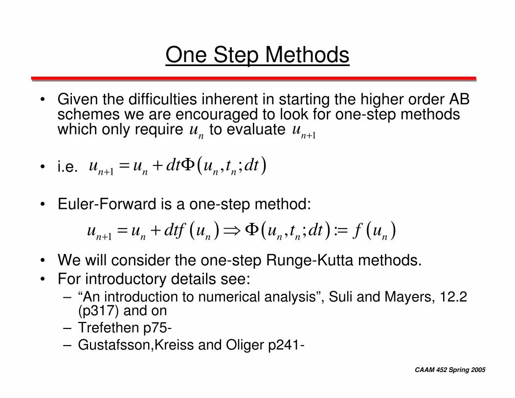
One Step Methods
• Given the difficulties inherent in starting the higher order AB schemes we are encouraged to look for one-step methods which only require to evaluate
• i.e.
• Euler-Forward is a one-step method:
• We will consider the one-step Runge-Kutta methods.• For introductory details see:
– “An introduction to numerical analysis”, Suli and Mayers, 12.2 (p317) and on
– Trefethen p75-– Gustafsson,Kreiss and Oliger p241-
nu 1nu +
( )1 , ;n n n nu u dt u t dt+ = + Φ
( ) ( ) ( )1 , ; :n n n n n nu u dtf u u t dt f u+ = + � Φ =
CAAM 452 Spring 2005
Runge-Kutta Methods
• The Runge-Kutta are a family of one-step methods.
• They consist of s stages (i.e. require s evaluations of f)
• They will be p’th order accurate, for some p.
• They are self starting !!!.
CAAM 452 Spring 2005
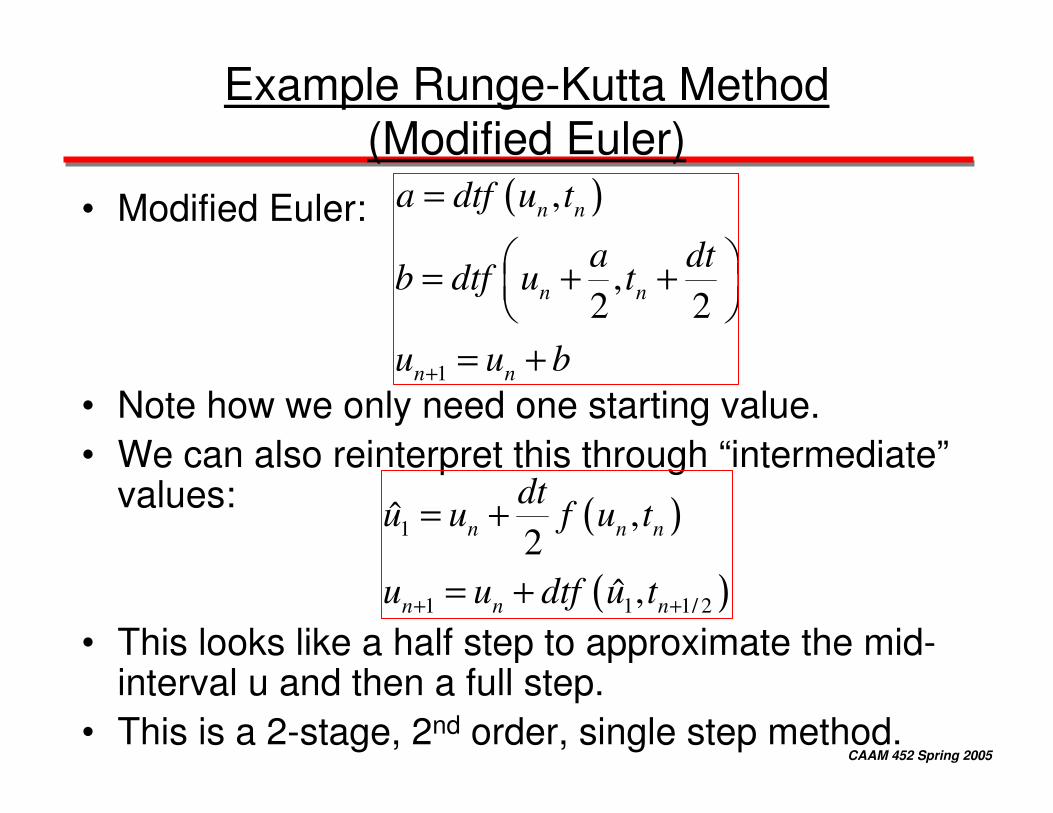
Example Runge-Kutta Method (Modified Euler)
• Modified Euler:
• Note how we only need one starting value.• We can also reinterpret this through “intermediate”
values:
• This looks like a half step to approximate the mid-interval u and then a full step.
• This is a 2-stage, 2nd order, single step method.
( )
1
,
,2 2
n n
n n
n n
a dtf u t
a dtb dtf u t
u u b+
=
� �= + +� �� �
= +
( )
( )1
1 1 1/ 2
,ˆ2
,ˆ
n n n
n n n
dtu u f u t
u u dtf u t+ +
= +
= +
CAAM 452 Spring 2005
Linear Stability Analysis
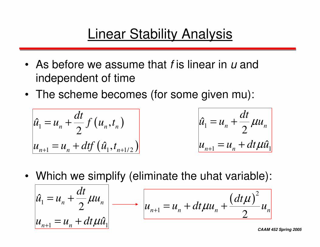
• As before we assume that f is linear in u and independent of time
• The scheme becomes (for some given mu):
• Which we simplify (eliminate the uhat variable):
( )
( )1
1 1 1/ 2
,ˆ2
,ˆ
n n n
n n n
dtu u f u t
u u dtf u t+ +
= +
= +
1
1 1
ˆ2
ˆ
n n
n n
dtu u u
u u dt u
µ
µ+
= +
= +
1
1 1
ˆ2
ˆ
n n
n n
dtu u u
u u dt u
µ
µ+
= +
= +
( )2
1 2n n n n
dtu u dt u u
µµ+ = + +
CAAM 452 Spring 2005
cont
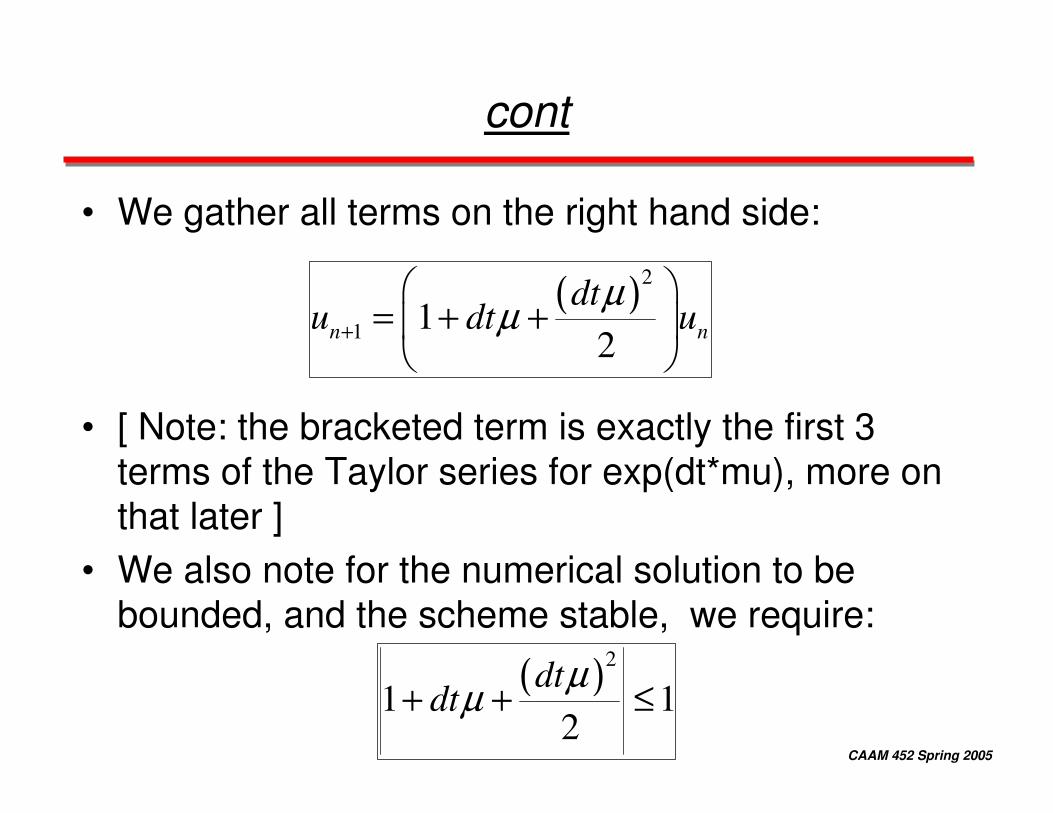
• We gather all terms on the right hand side:
• [ Note: the bracketed term is exactly the first 3 terms of the Taylor series for exp(dt*mu), more on that later ]
• We also note for the numerical solution to be bounded, and the scheme stable, we require:
( )2
1 12n n
dtu dt u
µµ+
� �= + +� �� �
( )2
1 12
dtdt
µµ+ + ≤
CAAM 452 Spring 2005
cont
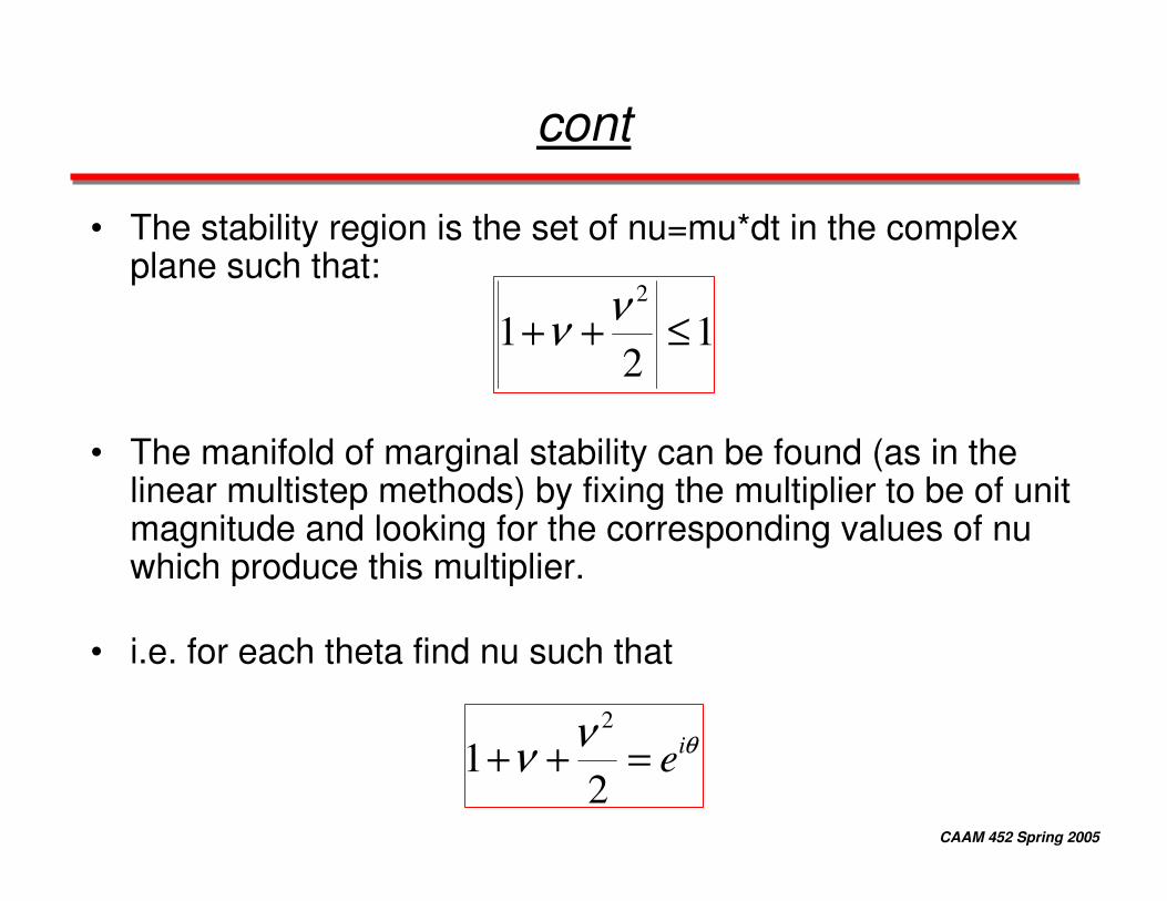
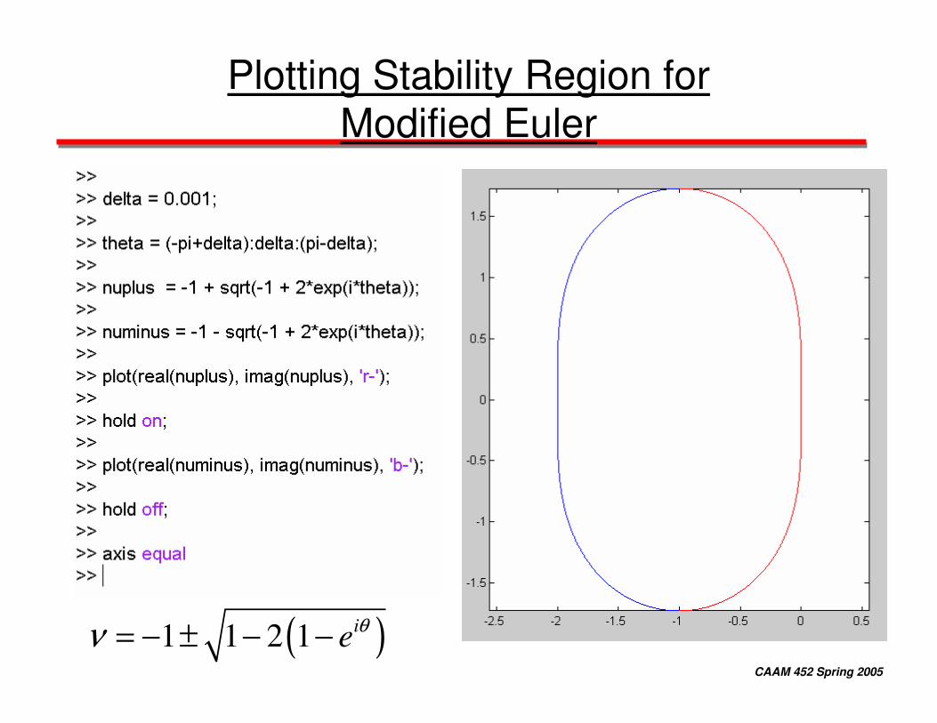
• The stability region is the set of nu=mu*dt in the complex plane such that:
• The manifold of marginal stability can be found (as in the linear multistep methods) by fixing the multiplier to be of unit magnitude and looking for the corresponding values of nuwhich produce this multiplier.
• i.e. for each theta find nu such that
2
1 12
νν+ + ≤
2
12
ie θνν+ + =
CAAM 452 Spring 2005
cont
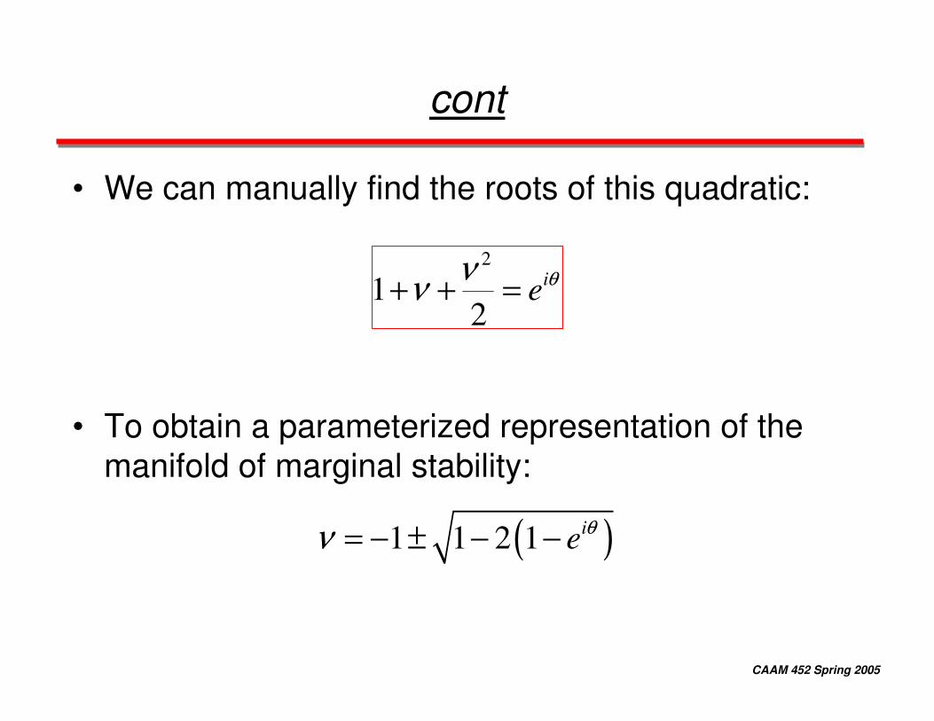
• We can manually find the roots of this quadratic:
• To obtain a parameterized representation of the manifold of marginal stability:
2
12
ie θνν+ + =
( )1 1 2 1 ie θν = − ± − −
CAAM 452 Spring 2005
Plotting Stability Region for Modified Euler
( )1 1 2 1 ie θν = − ± − −
CAAM 452 Spring 2005
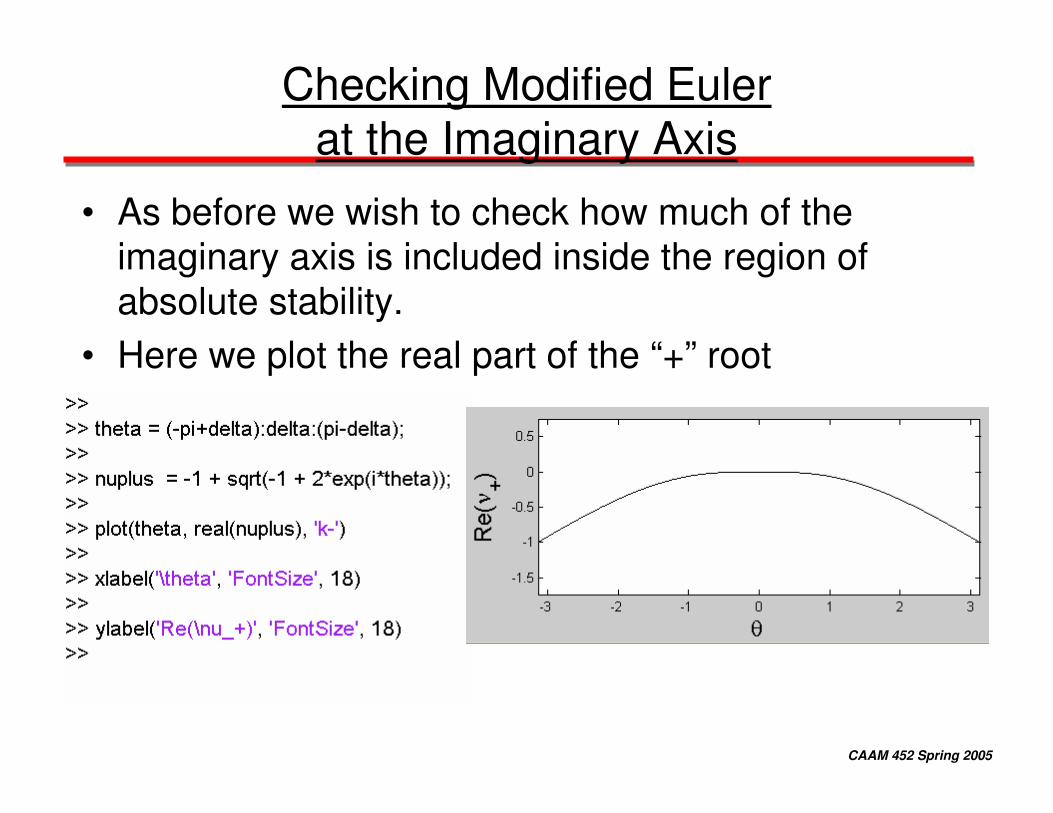
Checking Modified Euler at the Imaginary Axis
• As before we wish to check how much of the imaginary axis is included inside the region of absolute stability.
• Here we plot the real part of the “+” root
CAAM 452 Spring 2005
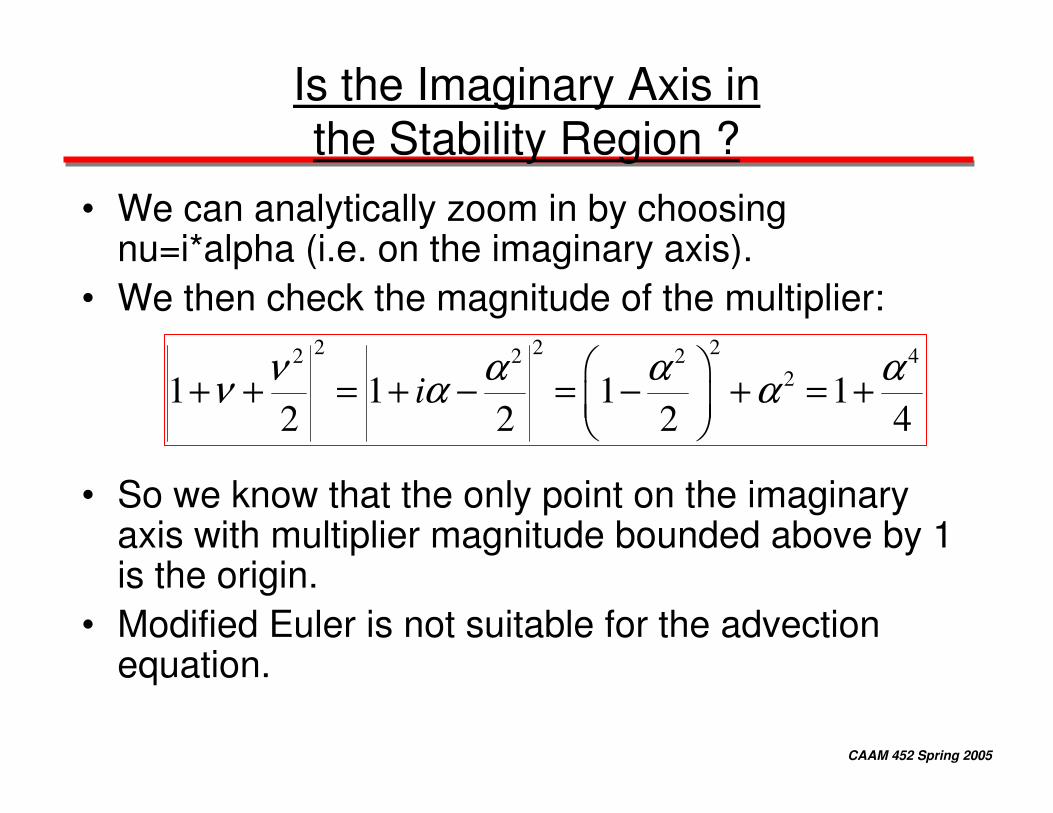
Is the Imaginary Axis in the Stability Region ?
• We can analytically zoom in by choosing nu=i*alpha (i.e. on the imaginary axis).
• We then check the magnitude of the multiplier:
• So we know that the only point on the imaginary axis with multiplier magnitude bounded above by 1 is the origin.
• Modified Euler is not suitable for the advection equation.
2 2 22 2 2 421 1 1 1
2 2 2 4i
ν α α αν α α� �+ + = + − = − + = +� �� �
CAAM 452 Spring 2005
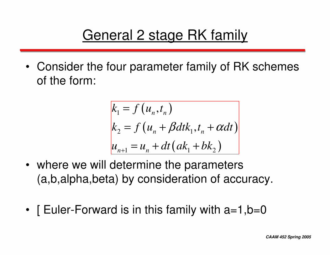
General 2 stage RK family
• Consider the four parameter family of RK schemes of the form:
• where we will determine the parameters (a,b,alpha,beta) by consideration of accuracy.
• [ Euler-Forward is in this family with a=1,b=0
( )( )
( )
1
2 1
1 1 2
,
,n n
n n
n n
k f u t
k f u dtk t dt
u u dt ak bk
β α
+
== + +
= + +
CAAM 452 Spring 2005
cont
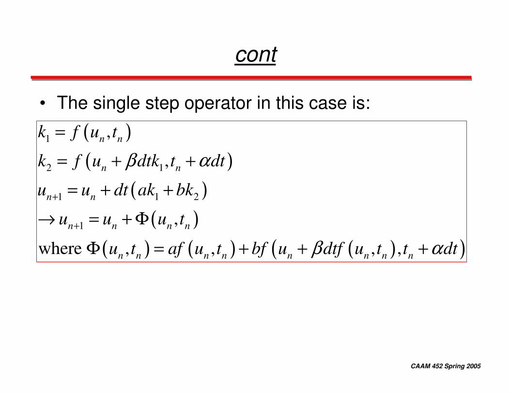
• The single step operator in this case is:
( )( )
( )( )
( ) ( ) ( )( )
1
2 1
1 1 2
1
,
,
,
where , , , ,
n n
n n
n n
n n n n
n n n n n n n n
k f u t
k f u dtk t dt
u u dt ak bk
u u u t
u t af u t bf u dtf u t t dt
β α
β α
+
+
== + +
= + +→ = + Φ
Φ = + + +
CAAM 452 Spring 2005
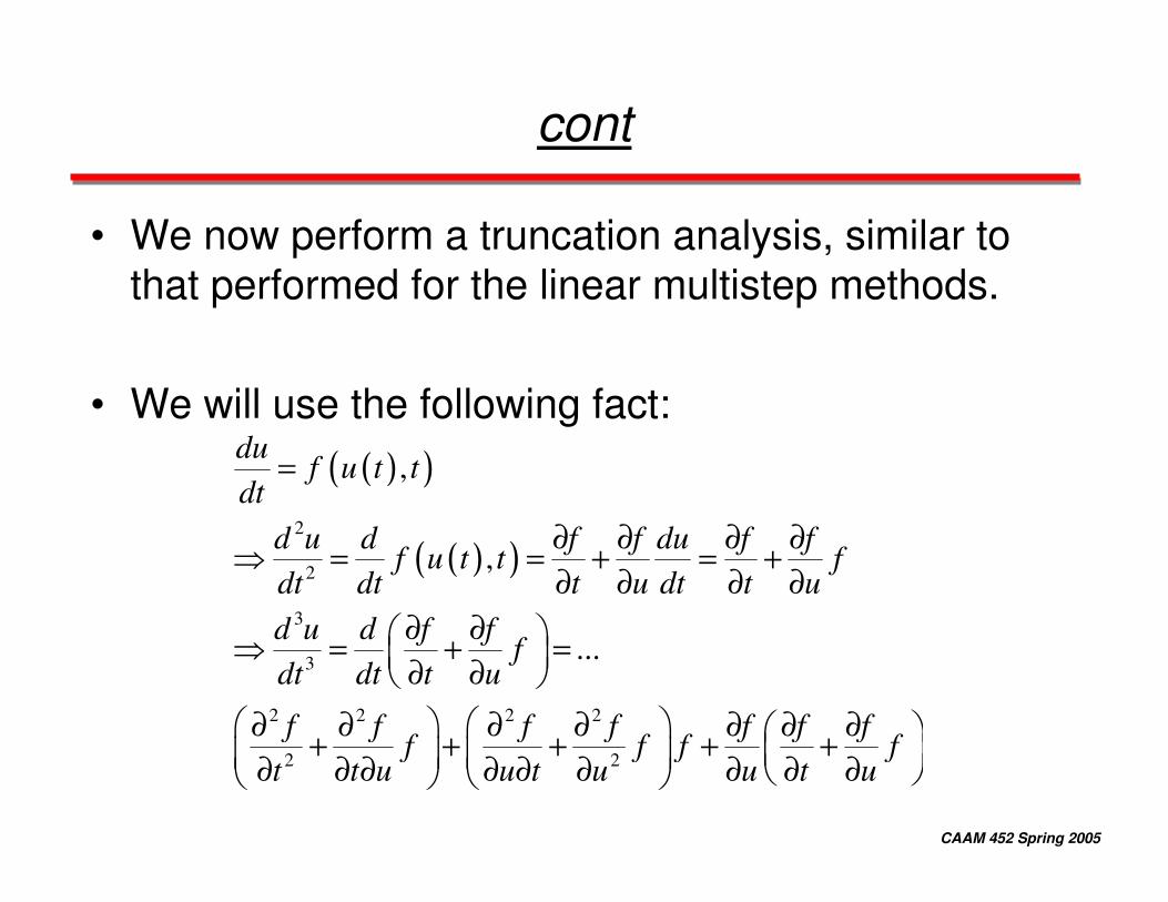
cont
• We now perform a truncation analysis, similar to that performed for the linear multistep methods.
• We will use the following fact:( )( )
( )( )2
2
3
3
2 2 2 2
2 2
,
,
...
duf u t t
dtd u d f f du f f
f u t t fdt dt t u dt t ud u d f f
fdt dt t u
f f f f f f ff f f f
t t u u t u u t u
=
∂ ∂ ∂ ∂� = = + = +
∂ ∂ ∂ ∂∂ ∂� �� = + =� �∂ ∂� �
� � � �∂ ∂ ∂ ∂ ∂ ∂ ∂� �+ + + + +� �� � � �∂ ∂ ∂ ∂ ∂ ∂ ∂ ∂ ∂� �� � � �
CAAM 452 Spring 2005
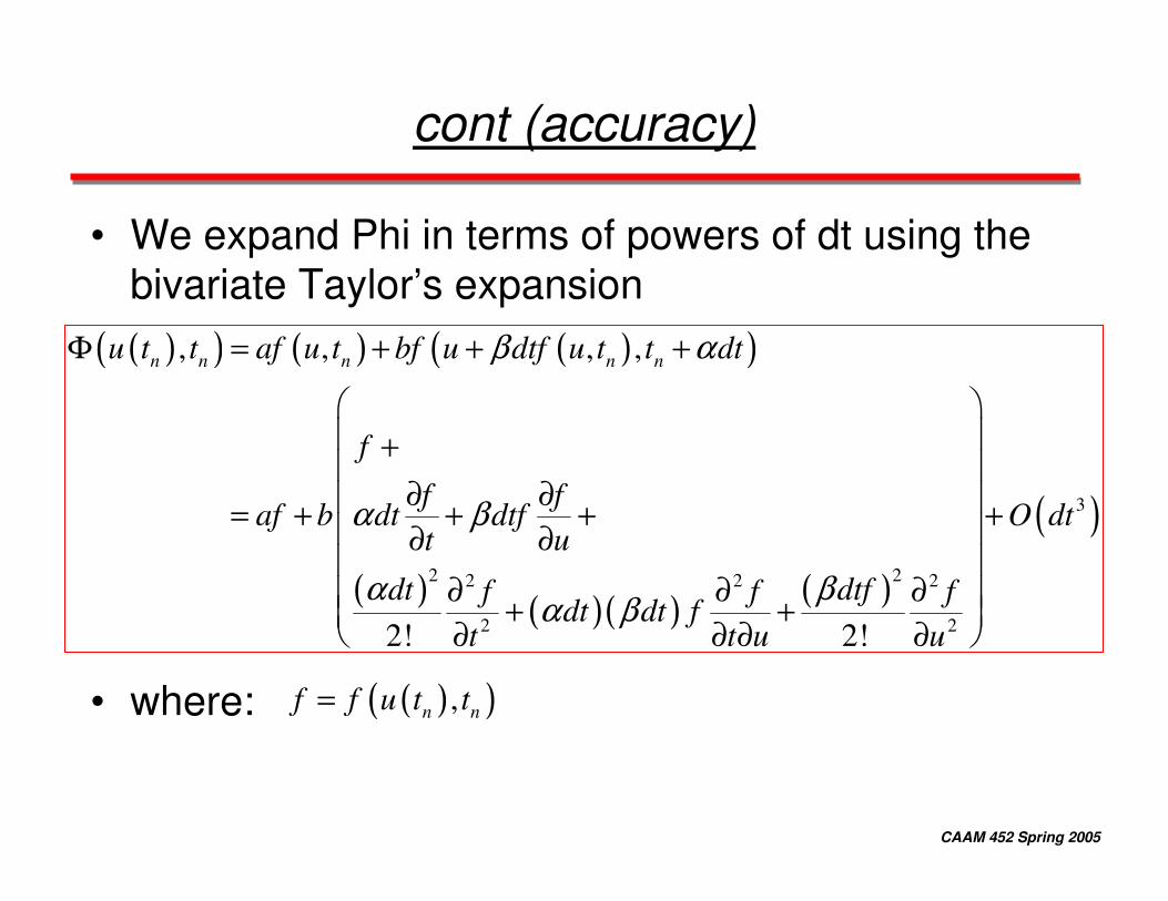
cont (accuracy)
• We expand Phi in terms of powers of dt using the bivariate Taylor’s expansion
• where:
( )( ) ( ) ( )( )
( ) ( )( ) ( )
( )3
2 22 2 2
2 2
, , , ,
2! 2!
n n n n nu t t af u t bf u dtf u t t dt
f
f faf b dt dtf O dt
t u
dt dtff f fdt dt f
t t u u
β α
α β
α βα β
Φ = + + +
� �� �+� �
∂ ∂� �= + + + +� �∂ ∂� �
∂ ∂ ∂� �+ +� �� �∂ ∂ ∂ ∂
( )( ),n nf f u t t=
CAAM 452 Spring 2005
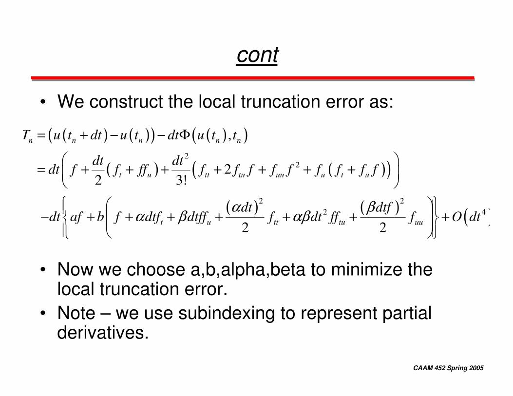
cont
• We construct the local truncation error as:
• Now we choose a,b,alpha,beta to minimize the local truncation error.
• Note – we use subindexing to represent partial derivatives.
( ) ( )( ) ( )( )
( ) ( )( )
( ) ( ) ( )
22
2 22 4
,
22 3!
2 2
n n n n n
t u tt tu uu u t u
t u tt tu uu
T u t dt u t dt u t t
dt dtdt f f ff f f f f f f f f f
dt dtfdt af b f dtf dtff f dt ff f O dt
α βα β αβ
= + − − Φ
� �= + + + + + + +� �� �
� �� �− + + + + + + +� �� � �� �� �� �
CAAM 452 Spring 2005
cont
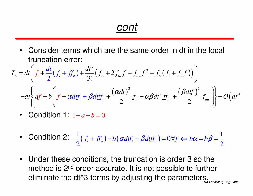
• Consider terms which are the same order in dt in the local truncation error:
• Condition 1:
• Condition 2:
• Under these conditions, the truncation is order 3 so the method is 2nd order accurate. It is not possible to further eliminate the dt^3 terms by adjusting the parameters.
( ) ( )( )
( ) ( ) ( )
22
2 22 4
23
2
2 !
2
n tt tu uu u t u
tt
t u
t u tu uu
dtf ff
d
dtf
f f
T dt f f f f f f f f f
dt dtfdt a b f dt fftf dtff f O dt
αα β βαβ
� �= + + + + + +� �� �
� �� �− + + + + + +� �� � �� �� �� �
+
+
1 0a b− − =
( ) ( )1 10
2 2t u t uf ff b dtf dtff f b bα β α β+ − + = ∀ ⇔ = =
CAAM 452 Spring 2005
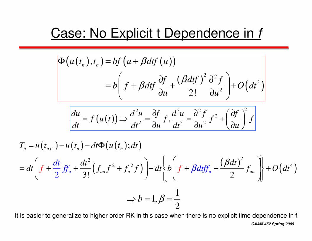
Case: No Explicit t Dependence in f
( )( ) ( )( )( ) ( )
2 23
2
,
2!
n nu t t bf u dtf u
dtff fb f dtf O dt
u u
β
ββ
Φ = +
� �∂ ∂= + + +� �∂ ∂� �
( )( )22 3 2
22 3 2,
du d u f d u f ff u t f f f
dt dt u dt u u∂ ∂ ∂� �= � = = +� �∂ ∂ ∂� �
( ) ( ) ( )( )
( ) ( ) ( )
1
222 2 4
;
3! 22
n n n n
uu uuu uu
T u t u t dt u t dt
dtdtdt f f f f dt b f O d
dtff f ff tdtf β β
+= − − Φ
� �� � � �= + + + − + + +� �� � � � �� � � �� �� �
11,
2b β� = =
It is easier to generalize to higher order RK in this case when there is no explicit time dependence in f.
CAAM 452 Spring 2005
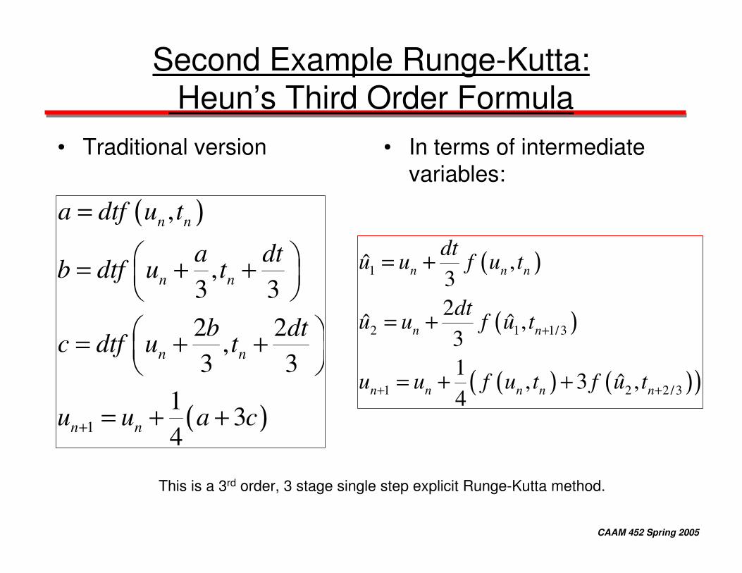
Second Example Runge-Kutta:Heun’s Third Order Formula
• Traditional version • In terms of intermediate variables:
( )
( )1
,
,3 32 2
,3 3
13
4
n n
n n
n n
n n
a dtf u t
a dtb dtf u t
b dtc dtf u t
u u a c+
=
� �= + +� �� �
� �= + +� �� �
= + +
( )
( )
( ) ( )( )
1
2 1 1/3
1 2 2/3
,ˆ32
,ˆ ˆ31
, 3 ,ˆ4
n n n
n n
n n n n n
dtu u f u t
dtu u f u t
u u f u t f u t
+
+ +
= +
= +
= + +
This is a 3rd order, 3 stage single step explicit Runge-Kutta method.
CAAM 452 Spring 2005
( ) ( )
1
2
1
2 3
ˆ32
ˆ3 3
23
4 3 3
23 1 1
4 3 3
12 3
n n
n n n
n n n n n n
n n
n
dtu u u
dt dtu u u u
dt dt dtu u u u u u
dt dt dtu u
dt dtdt u
µ
µ µ
µ µ µ µ
µ µ µ µ
µ µµ
+
= +
� �= + +� �� �
� �� �� �= + + + +� �� �� �� �� �� �
� �� �� �= + + + +� �� �� �� �� �� �
� �= + + +� �� �� �
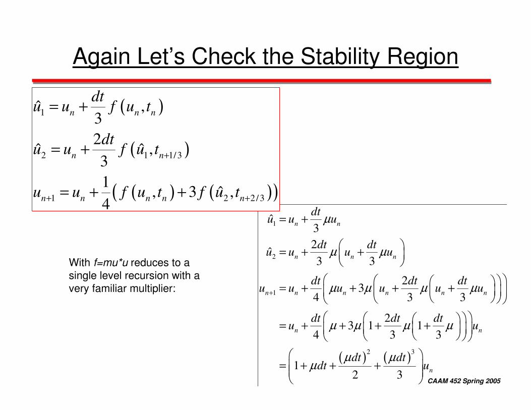
Again Let’s Check the Stability Region
( )
( )
( ) ( )( )
1
2 1 1/3
1 2 2/3
,ˆ32
,ˆ ˆ31
, 3 ,ˆ4
n n n
n n
n n n n n
dtu u f u t
dtu u f u t
u u f u t f u t
+
+ +
= +
= +
= + +
With f=mu*u reduces to a single level recursion with a very familiar multiplier:
CAAM 452 Spring 2005
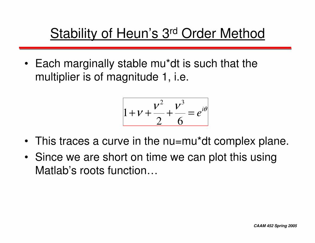
Stability of Heun’s 3rd Order Method
• Each marginally stable mu*dt is such that the multiplier is of magnitude 1, i.e.
• This traces a curve in the nu=mu*dt complex plane. • Since we are short on time we can plot this using
Matlab’s roots function…
2 3
12 6
ie θν νν+ + + =
CAAM 452 Spring 2005
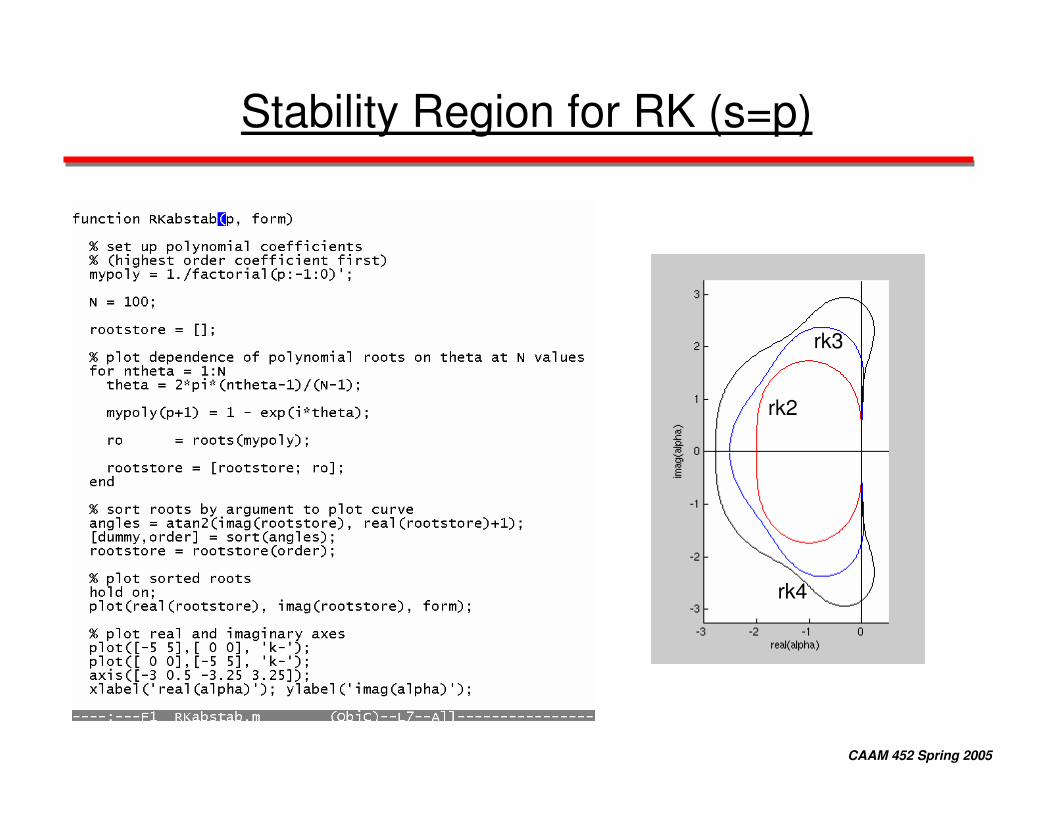
Stability Region for RK (s=p)
rk2
rk3
rk4
CAAM 452 Spring 2005
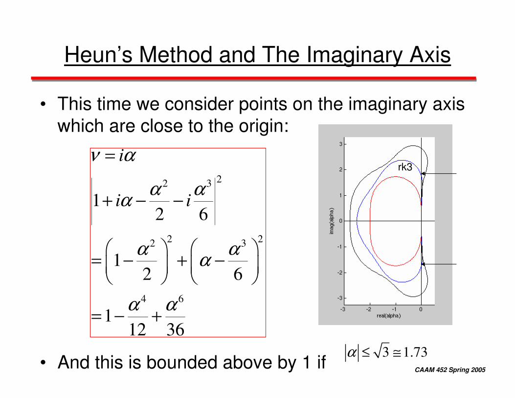
• This time we consider points on the imaginary axis which are close to the origin:
• And this is bounded above by 1 if
Heun’s Method and The Imaginary Axis
22 3
2 22 3
4 6
12 6
12 6
112 36
i
i i
ν α
α αα
α αα
α α
=
+ − −
� � � �= − + −� � � �� � � �
= − +
3 1.73α ≤ ≅
rk3
CAAM 452 Spring 2005
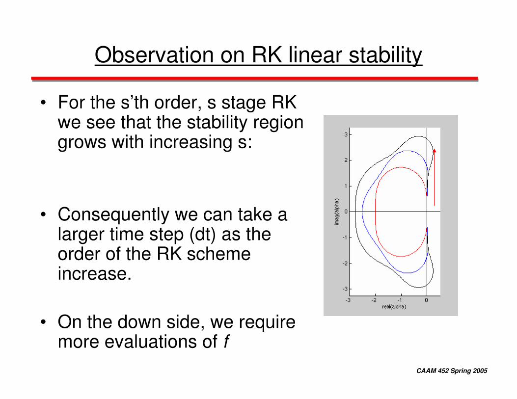
Observation on RK linear stability
• For the s’th order, s stage RK we see that the stability region grows with increasing s:
• Consequently we can take a larger time step (dt) as the order of the RK scheme increase.
• On the down side, we require more evaluations of f
CAAM 452 Spring 2005
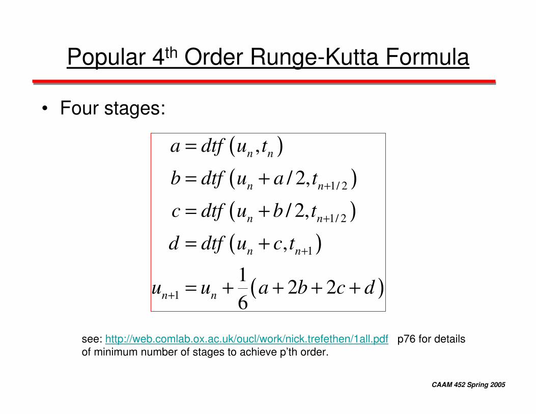
Popular 4th Order Runge-Kutta Formula
• Four stages:
( )( )( )( )
( )
1/ 2
1/ 2
1
1
,
/ 2,
/ 2,
,
12 2
6
n n
n n
n n
n n
n n
a dtf u t
b dtf u a t
c dtf u b t
d dtf u c t
u u a b c d
+
+
+
+
== += += +
= + + + +
see: http://web.comlab.ox.ac.uk/oucl/work/nick.trefethen/1all.pdf p76 for detailsof minimum number of stages to achieve p’th order.
CAAM 452 Spring 2005
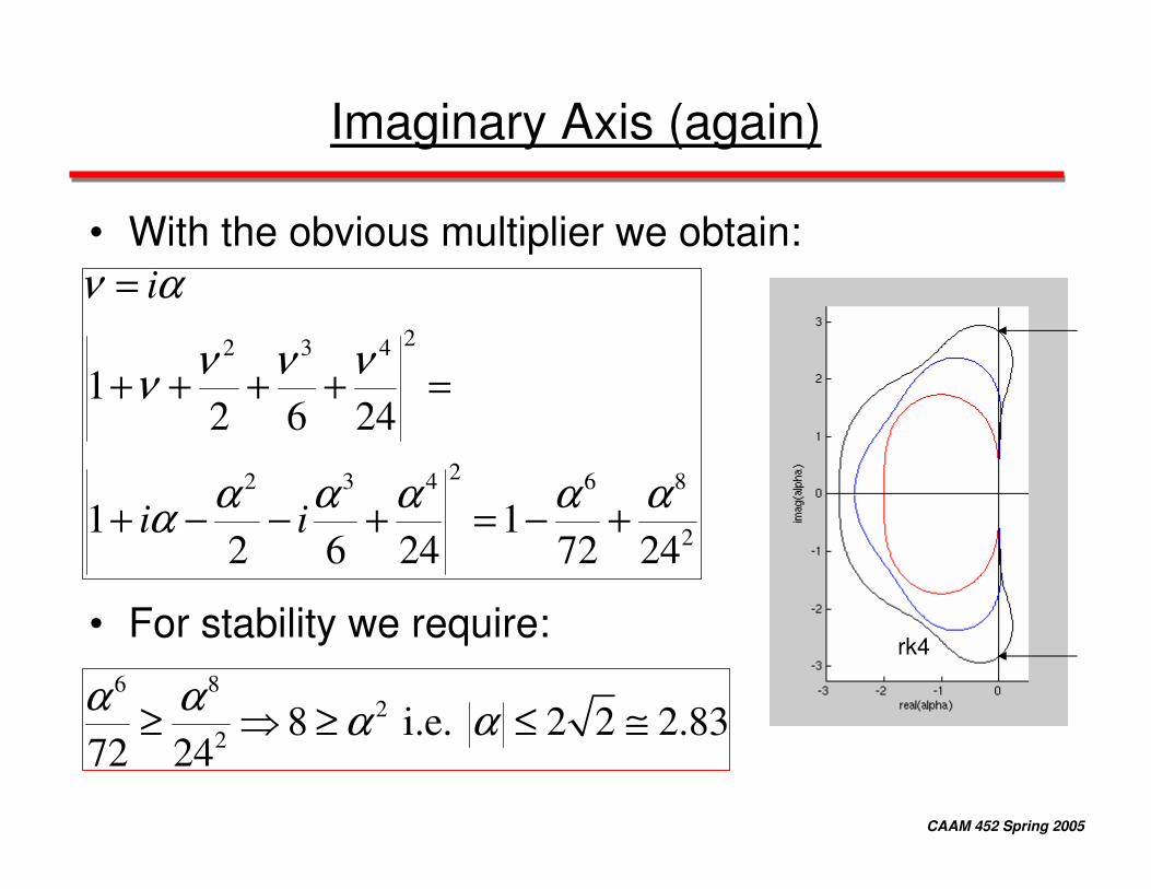
Imaginary Axis (again)
• With the obvious multiplier we obtain:
• For stability we require:
22 3 4
22 3 4 6 8
2
12 6 24
1 12 6 24 72 24
i
i i
ν α
ν ν νν
α α α α αα
=
+ + + + =
+ − − + = − +
6 82
2 8 i.e. 2 2 2.8372 24α α α α≥ � ≥ ≤ ≅
rk4
CAAM 452 Spring 2005
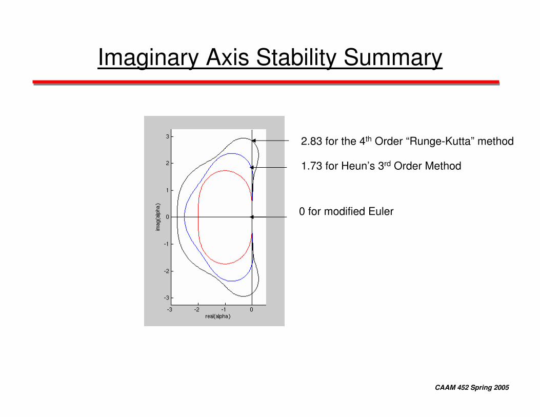
Imaginary Axis Stability Summary
2.83 for the 4th Order “Runge-Kutta” method
1.73 for Heun’s 3rd Order Method
0 for modified Euler
CAAM 452 Spring 2005
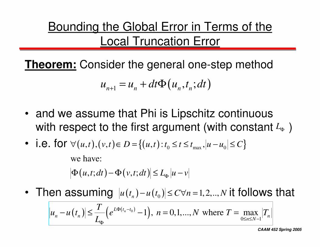
Bounding the Global Error in Terms of the Local Truncation Error
Theorem: Consider the general one-step method
• and we assume that Phi is Lipschitz continuous with respect to the first argument (with constant )
• i.e. for
• Then assuming it follows that
( )1 , ;n n n nu u dt u t dt+ = + Φ
LΦ
( ) ( ) ( ){ }
( ) ( )
0 max 0, , , , : ,
we have:
, ; , ;
u t v t D u t t t t u u C
u t dt v t dt L u vΦ
∀ ∈ = ≤ ≤ − ≤
Φ − Φ ≤ −
( ) ( )0 1,2,..,nu t u t C n N− ≤ ∀ =
( ) ( )( )0
0 11 , 0,1,..., where maxnL t t
n n nn N
Tu u t e n N T T
LΦ −
≤ ≤ −Φ
− ≤ − = =
CAAM 452 Spring 2005
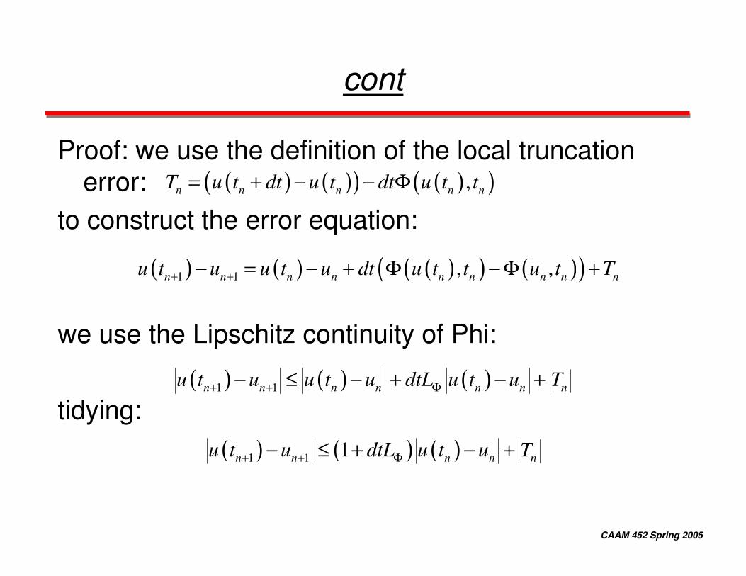
cont
Proof: we use the definition of the local truncation error:
to construct the error equation:
we use the Lipschitz continuity of Phi:
tidying:
( ) ( )( ) ( )( ),n n n n nT u t dt u t dt u t t= + − − Φ
( ) ( ) ( )( ) ( )( )1 1 , ,n n n n n n n n nu t u u t u dt u t t u t T+ +− = − + Φ − Φ +
( ) ( ) ( )1 1n n n n n n nu t u u t u dtL u t u T+ + Φ− ≤ − + − +
( ) ( ) ( )1 1 1n n n n nu t u dtL u t u T+ + Φ− ≤ + − +
CAAM 452 Spring 2005
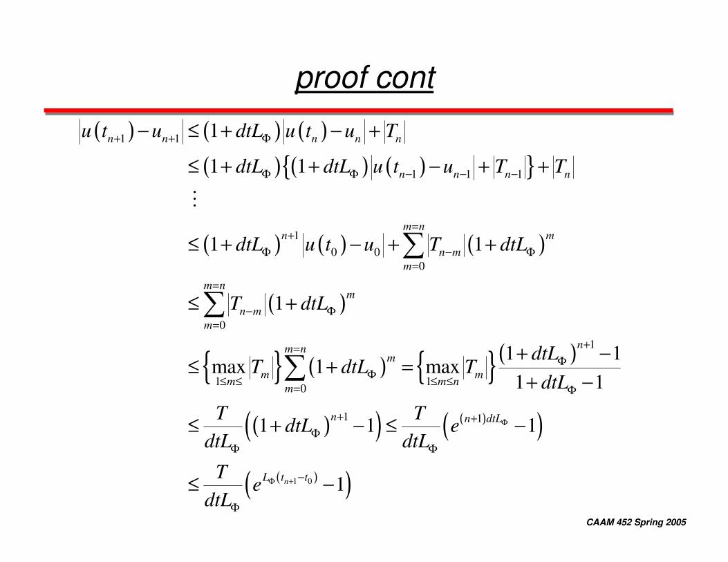
proof cont
( ) ( ) ( )( ) ( ) ( ){ }
( ) ( ) ( )
( )
{ } ( ) { }( )
( )( ) ( )( )
1 1
1 1 1
10 0
0
0
1
1 10
1 1
1
1 1
1 1
1
1 1max 1 max
1 1
1 1 1
n n n n n
n n n n
m nn m
n mm
m nm
n mm
nm nm
m mm m nm
n n dtL
u t u dtL u t u T
dtL dtL u t u T T
dtL u t u T dtL
T dtL
dtLT dtL T
dtL
T TdtL e
dtL dtLΦ
+ + Φ
Φ Φ − − −
=+
Φ − Φ=
=
− Φ=
+=Φ
Φ≤ ≤ ≤ ≤= Φ
+ +Φ
Φ Φ
− ≤ + − +
≤ + + − + +
≤ + − + +
≤ +
+ −≤ + =
+ −
≤ + − ≤ −
≤
�
�
�
�
( )( )1 0 1nL t tTe
dtLΦ + −
Φ
−
CAAM 452 Spring 2005
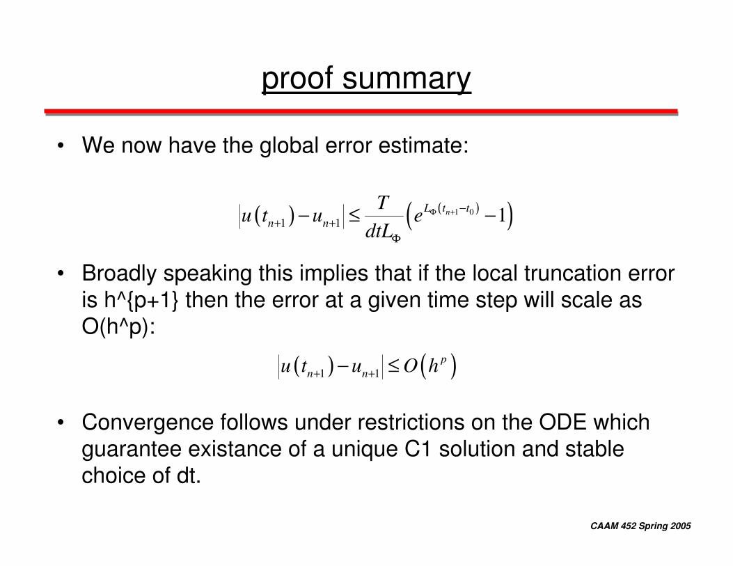
proof summary
• We now have the global error estimate:
• Broadly speaking this implies that if the local truncation erroris h^{p+1} then the error at a given time step will scale as O(h^p):
• Convergence follows under restrictions on the ODE which guarantee existance of a unique C1 solution and stable choice of dt.
( ) ( )( )1 01 1 1nL t t
n n
Tu t u e
dtLΦ + −
+ +Φ
− ≤ −
( ) ( )1 1p
n nu t u O h+ +− ≤
CAAM 452 Spring 2005
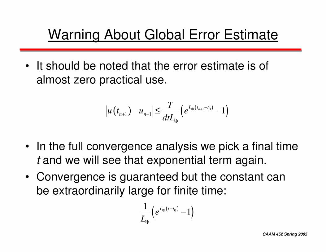
Warning About Global Error Estimate
• It should be noted that the error estimate is of almost zero practical use.
• In the full convergence analysis we pick a final time t and we will see that exponential term again.
• Convergence is guaranteed but the constant can be extraordinarily large for finite time:
( ) ( )( )1 01 1 1nL t t
n n
Tu t u e
dtLΦ + −
+ +Φ
− ≤ −
( )( )01
1L t teL
Φ −
Φ
−
CAAM 452 Spring 2005
A Posteriori Error Estimate
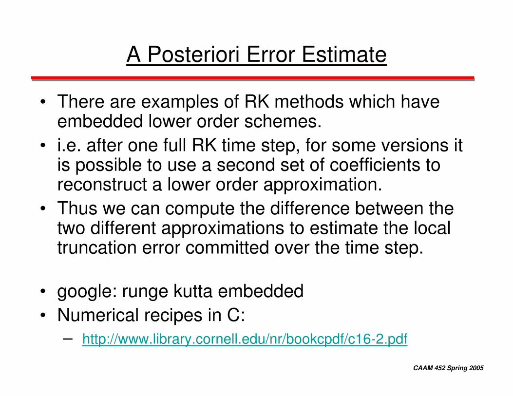
• There are examples of RK methods which have embedded lower order schemes.
• i.e. after one full RK time step, for some versions it is possible to use a second set of coefficients to reconstruct a lower order approximation.
• Thus we can compute the difference between the two different approximations to estimate the local truncation error committed over the time step.
• google: runge kutta embedded • Numerical recipes in C:
– http://www.library.cornell.edu/nr/bookcpdf/c16-2.pdf
CAAM 452 Spring 2005
My Favorite s StageRunge-Kutta Method
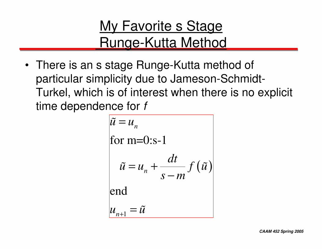
• There is an s stage Runge-Kutta method of particular simplicity due to Jameson-Schmidt-Turkel, which is of interest when there is no explicit time dependence for f
( )
1
for m=0:s-1
end
n
n
n
u u
dtu u f u
s m
u u+
=
= +−
=
�
� �
�
CAAM 452 Spring 2005
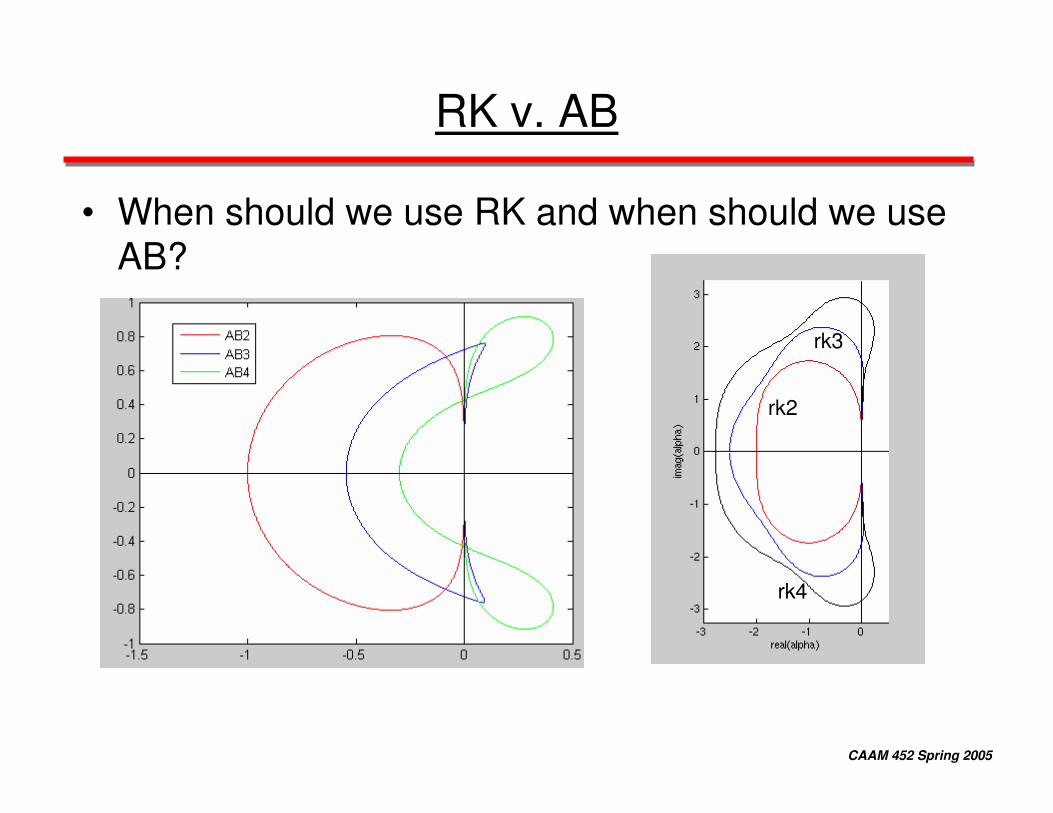
RK v. AB
• When should we use RK and when should we use AB?
rk2
rk3
rk4

CAAM 452 Spring 2005
Class Cancelled on 02/17/05
• There will be no class on Thursday 02/17/05
• The homework due for that class will be due the following Thursday 02/24/05