Numerical computation of partial differential equation 2fluid.web.nitech.ac.jp/Gotoh_Home_page/Edu/Under_Graduate_course/... · Numerical computation of partial differential equation

Nagoya Institute of Technology

Numerical computation of partial differential equation 2


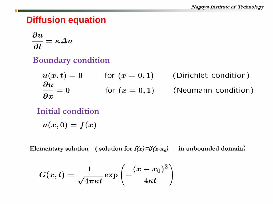
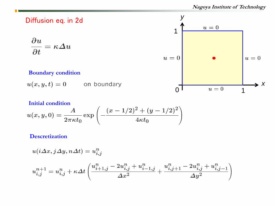
Diffusion equation

Boundary condition

Initial condition

Elementary solution ( solution for f(x)=d(x-x0) in unbounded domain）


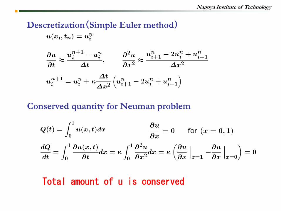
Conserved quantity for Neuman problem

Descretization（Simple Euler method）

Total amount of u is conserved


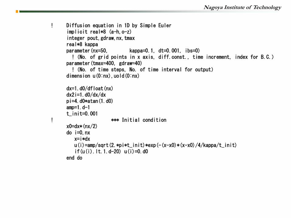
! Diffusion equation in 1D by Simple Euler implicit real*8 (a-h,o-z) integer pout,gdraw,nx,tmax real*8 kappa parameter(nx=50, kappa=0.1, dt=0.001, ibs=0) !（No. of grid points in x axis, diff.const., time increment, index for B.C.） parameter(tmax=400, gdraw=40) !（No. of time steps, No. of time interval for output） dimension u(0:nx),uold(0:nx) dx=1.d0/dfloat(nx) dx2i=1.d0/dx/dx pi=4.d0*atan(1.d0) amp=1.d-1 t_init=0.001 ! *** Initial condition x0=dx*(nx/2) do i=0,nx x=i*dx u(i)=amp/sqrt(2.*pi*t_init)*exp(-(x-x0)*(x-x0)/4/kappa/t_init) if(u(i).lt.1.d-20) u(i)=0.d0 end do


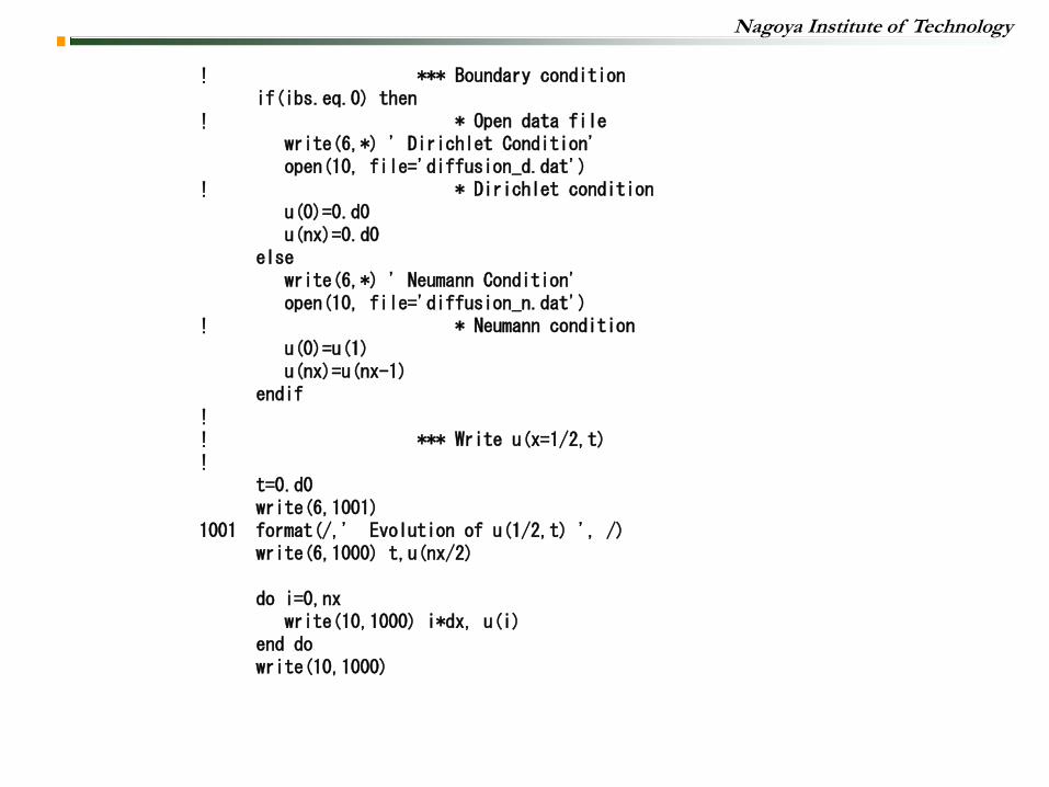
! *** Boundary condition if(ibs.eq.0) then ! * Open data file write(6,*) ' Dirichlet Condition' open(10, file='diffusion_d.dat') ! * Dirichlet condition u(0)=0.d0 u(nx)=0.d0 else write(6,*) ' Neumann Condition' open(10, file='diffusion_n.dat') ! * Neumann condition u(0)=u(1) u(nx)=u(nx-1) endif ! ! *** Write u(x=1/2,t) ! t=0.d0 write(6,1001) 1001 format(/,' Evolution of u(1/2,t) ', /) write(6,1000) t,u(nx/2) do i=0,nx write(10,1000) i*dx, u(i) end do write(10,1000)


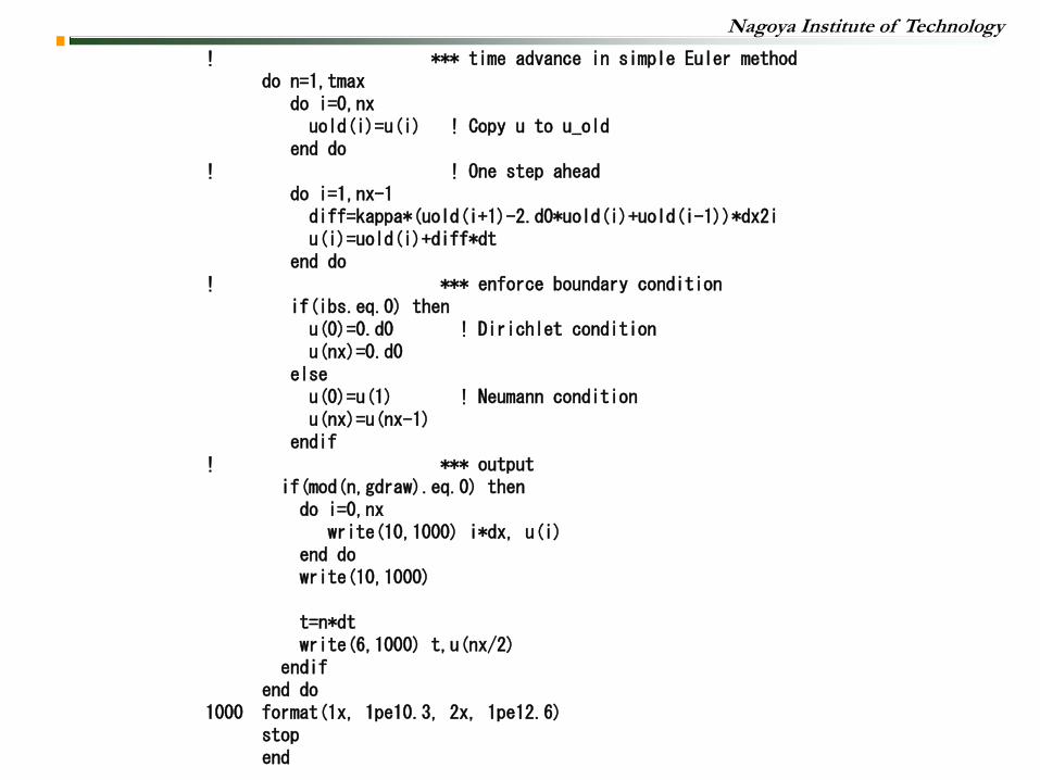
! *** time advance in simple Euler method do n=1,tmax do i=0,nx uold(i)=u(i) ! Copy u to u_old end do ! ! One step ahead do i=1,nx-1 diff=kappa*(uold(i+1)-2.d0*uold(i)+uold(i-1))*dx2i u(i)=uold(i)+diff*dt end do ! *** enforce boundary condition if(ibs.eq.0) then u(0)=0.d0 ! Dirichlet condition u(nx)=0.d0 else u(0)=u(1) ! Neumann condition u(nx)=u(nx-1) endif ! *** output if(mod(n,gdraw).eq.0) then do i=0,nx write(10,1000) i*dx, u(i) end do write(10,1000) t=n*dt write(6,1000) t,u(nx/2) endif end do 1000 format(1x, 1pe10.3, 2x, 1pe12.6) stop end



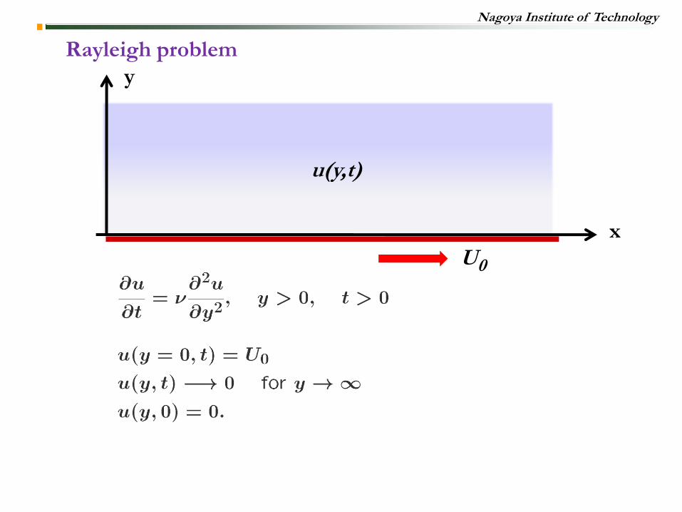
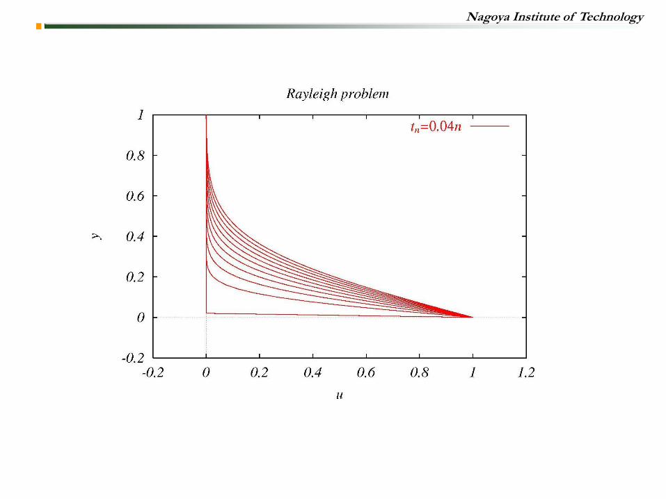
Rayleigh problem

x

y

U0

u(y,t)



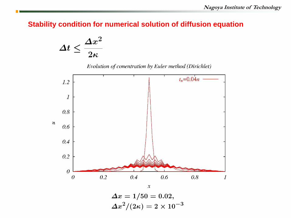
Stability condition for numerical solution of diffusion equation


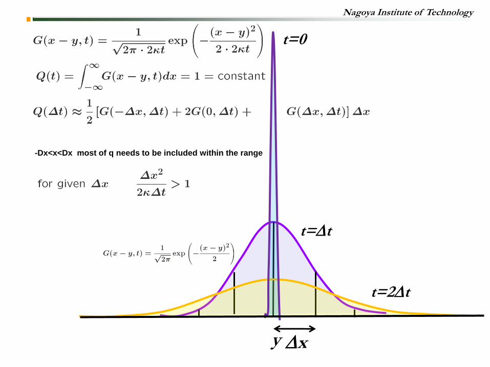
Dx

t=0

t=Dt

t=2Dt

-Dx<x<Dx most of q needs to be included within the range

y


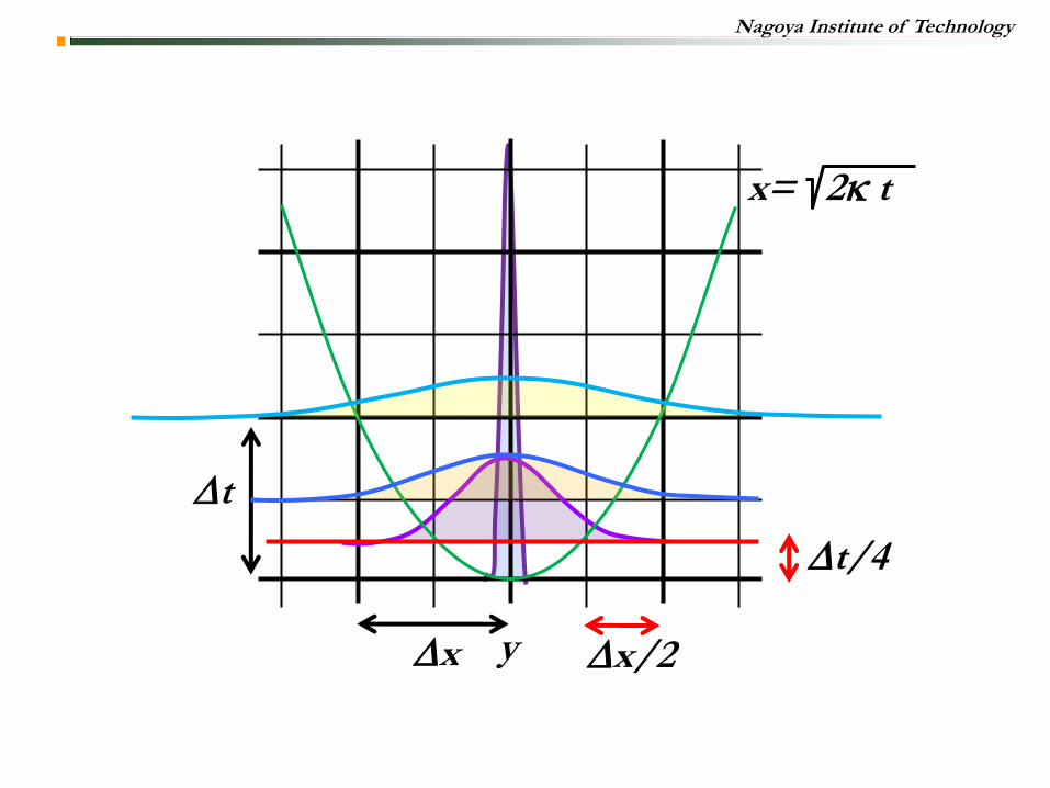
Dt

Dx

Dt/4

Dx/2

x= 2k t

y


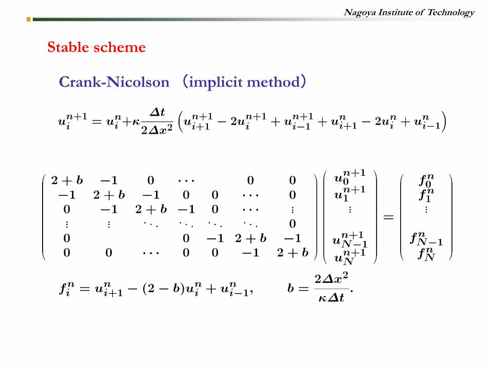
Stable scheme

Crank-Nicolson （implicit method）


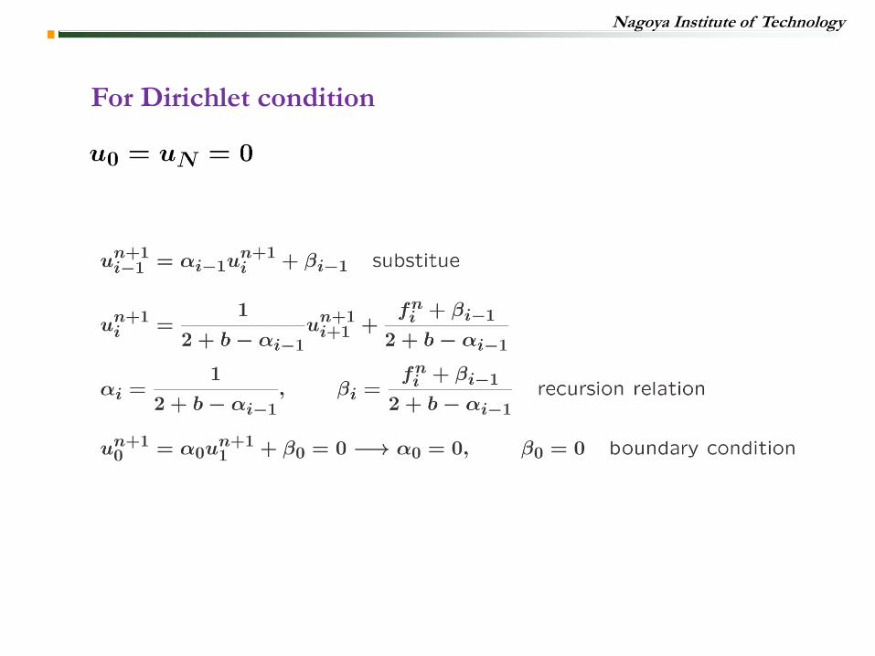
For Dirichlet condition


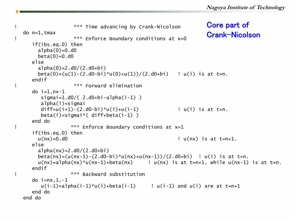
! *** Time advancing by Crank-Nicolson do n=1,tmax ! *** Enforce Boundary conditions at x=0 if(ibs.eq.0) then alpha(0)=0.d0 beta(0)=0.d0 else alpha(0)=2.d0/(2.d0+bi) beta(0)=(u(1)-(2.d0-bi)*u(0)+u(1))/(2.d0+bi) ! u(i) is at t=n. endif ! *** Forward elimination do i=1,nx-1 sigmai=1.d0/( 2.d0+bi-alpha(i-1) ) alpha(i)=sigmai diff=u(i+1)-(2.d0-bi)*u(i)+u(i-1) ! u(i) is at t=n. beta(i)=sigmai*( diff+beta(i-1) ) end do ! *** Enforce Boundary conditions at x=1 if(ibs.eq.0) then u(nx)=0.d0 ! u(nx) is at t=n+1. else alpha(nx)=2.d0/(2.d0+bi) beta(nx)=(u(nx-1)-(2.d0-bi)*u(nx)+u(nx-1))/(2.d0+bi) ! u(i) is at t=n. u(nx)=alpha(nx)*u(nx-1)+beta(nx) ! u(nx) is at t=n+1, while u(nx-1) is at t=n. endif ! *** Backward substitution do i=nx,1,-1 u(i-1)=alpha(i-1)*u(i)+beta(i-1) ! u(i-1) and u(i) are at t=n+1 end do end do

Core part of Crank-Nicolson


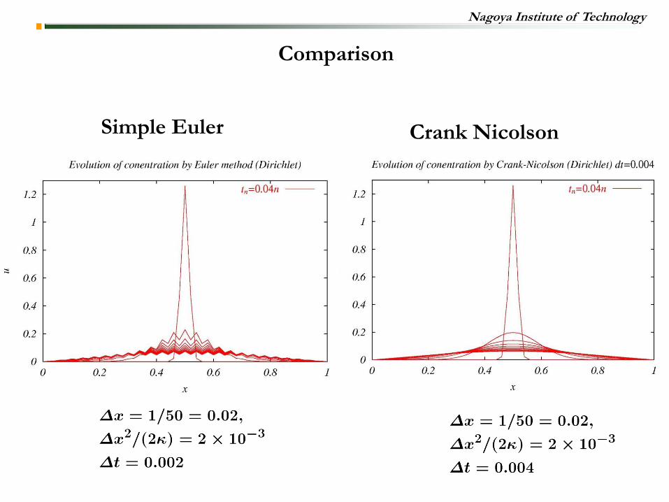
Comparison

Simple Euler Crank Nicolson


Diffusion eq. in 2d

Boundary condition

Initial condition

Descretization

1

1 0

y

x


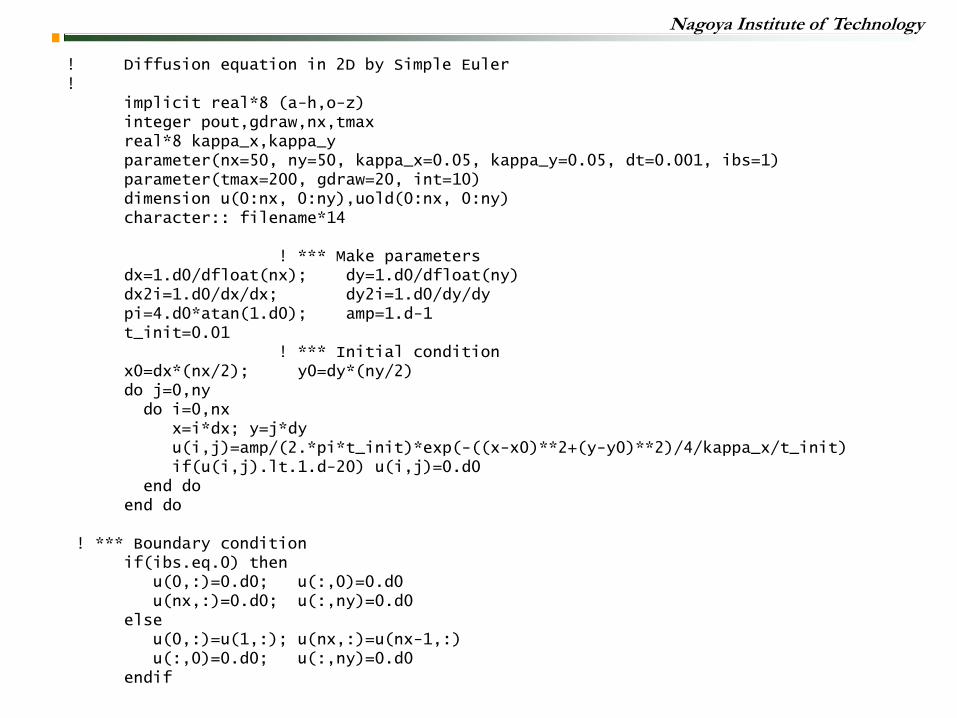
! Diffusion equation in 2D by Simple Euler ! implicit real*8 (a-h,o-z) integer pout,gdraw,nx,tmax real*8 kappa_x,kappa_y parameter(nx=50, ny=50, kappa_x=0.05, kappa_y=0.05, dt=0.001, ibs=1) parameter(tmax=200, gdraw=20, int=10) dimension u(0:nx, 0:ny),uold(0:nx, 0:ny) character:: filename*14 ! *** Make parameters dx=1.d0/dfloat(nx); dy=1.d0/dfloat(ny) dx2i=1.d0/dx/dx; dy2i=1.d0/dy/dy pi=4.d0*atan(1.d0); amp=1.d-1 t_init=0.01 ! *** Initial condition x0=dx*(nx/2); y0=dy*(ny/2) do j=0,ny do i=0,nx x=i*dx; y=j*dy u(i,j)=amp/(2.*pi*t_init)*exp(-((x-x0)**2+(y-y0)**2)/4/kappa_x/t_init) if(u(i,j).lt.1.d-20) u(i,j)=0.d0 end do end do ! *** Boundary condition if(ibs.eq.0) then u(0,:)=0.d0; u(:,0)=0.d0 u(nx,:)=0.d0; u(:,ny)=0.d0 else u(0,:)=u(1,:); u(nx,:)=u(nx-1,:) u(:,0)=0.d0; u(:,ny)=0.d0 endif


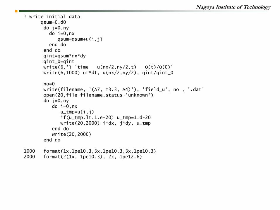
! write initial data qsum=0.d0 do j=0,ny do i=0,nx qsum=qsum+u(i,j) end do end do qint=qsum*dx*dy qint_0=qint write(6,*) 'time u(nx/2,ny/2,t) Q(t)/Q(0)' write(6,1000) nt*dt, u(nx/2,ny/2), qint/qint_0 no=0 write(filename, '(A7, I3.3, A4)'), 'field_u', no , '.dat' open(20,file=filename,status='unknown') do j=0,ny do i=0,nx u_tmp=u(i,j) if(u_tmp.lt.1.e-20) u_tmp=1.d-20 write(20,2000) i*dx, j*dy, u_tmp end do write(20,2000) end do 1000 format(1x,1pe10.3,3x,1pe10.3,3x,1pe10.3) 2000 format(2(1x, 1pe10.3), 2x, 1pe12.6)


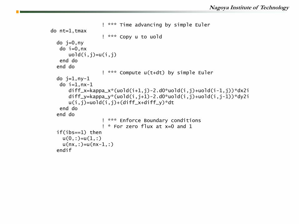
! *** Time advancing by simple Euler do nt=1,tmax ! *** Copy u to uold do j=0,ny do i=0,nx uold(i,j)=u(i,j) end do end do ! *** Compute u(t+dt) by simple Euler do j=1,ny-1 do i=1,nx-1 diff_x=kappa_x*(uold(i+1,j)-2.d0*uold(i,j)+uold(i-1,j))*dx2i diff_y=kappa_y*(uold(i,j+1)-2.d0*uold(i,j)+uold(i,j-1))*dy2i u(i,j)=uold(i,j)+(diff_x+diff_y)*dt end do end do ! *** Enforce Boundary conditions ! * For zero flux at x=0 and 1 if(ibs==1) then u(0,:)=u(1,:) u(nx,:)=u(nx-1,:) endif


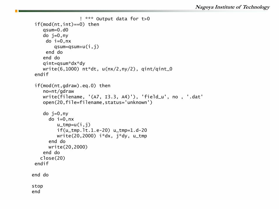
! *** Output data for t>0 if(mod(nt,int)==0) then qsum=0.d0 do j=0,ny do i=0,nx qsum=qsum+u(i,j) end do end do qint=qsum*dx*dy write(6,1000) nt*dt, u(nx/2,ny/2), qint/qint_0 endif if(mod(nt,gdraw).eq.0) then no=nt/gdraw write(filename, '(A7, I3.3, A4)'), 'field_u', no , '.dat' open(20,file=filename,status='unknown') do j=0,ny do i=0,nx u_tmp=u(i,j) if(u_tmp.lt.1.e-20) u_tmp=1.d-20 write(20,2000) i*dx, j*dy, u_tmp end do write(20,2000) end do close(20) endif end do stop end


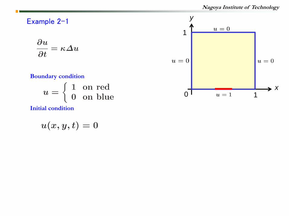
Example 2-1

Boundary condition

Initial condition

1

1 0

y

x


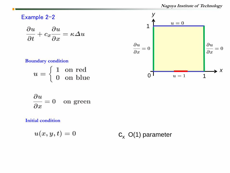
Example 2-2

1

1 0

y

x

cx O(1) parameter

Boundary condition

Initial condition


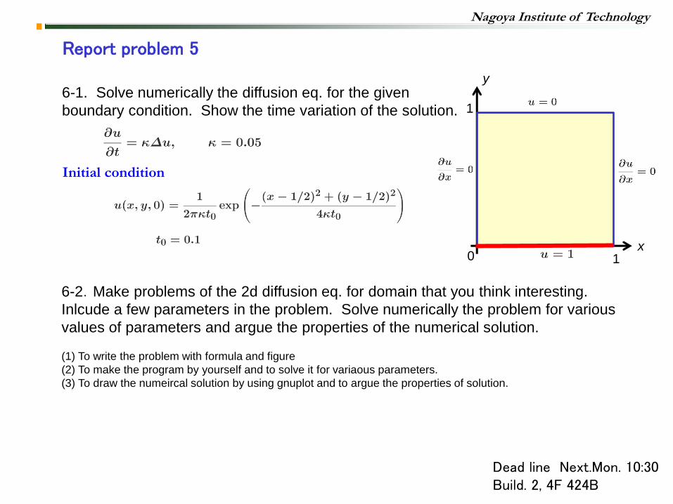
Report problem 5

6-1. Solve numerically the diffusion eq. for the given

boundary condition. Show the time variation of the solution. 1

1 0

y

x

6-2．Make problems of the 2d diffusion eq. for domain that you think interesting.

Inlcude a few parameters in the problem. Solve numerically the problem for various

values of parameters and argue the properties of the numerical solution.

(1) To write the problem with formula and figure

(2) To make the program by yourself and to solve it for variaous parameters.

(3) To draw the numeircal solution by using gnuplot and to argue the properties of solution.

Dead line Next.Mon. 10:30 Build. 2, 4F 424B

Initial condition


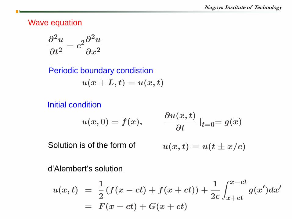
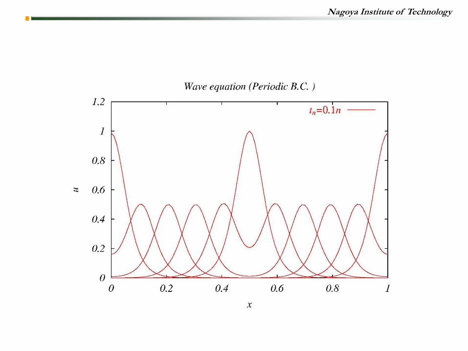
Wave equation

Periodic boundary condistion

Initial condition

Solution is of the form of

d‘Alembert‘s solution


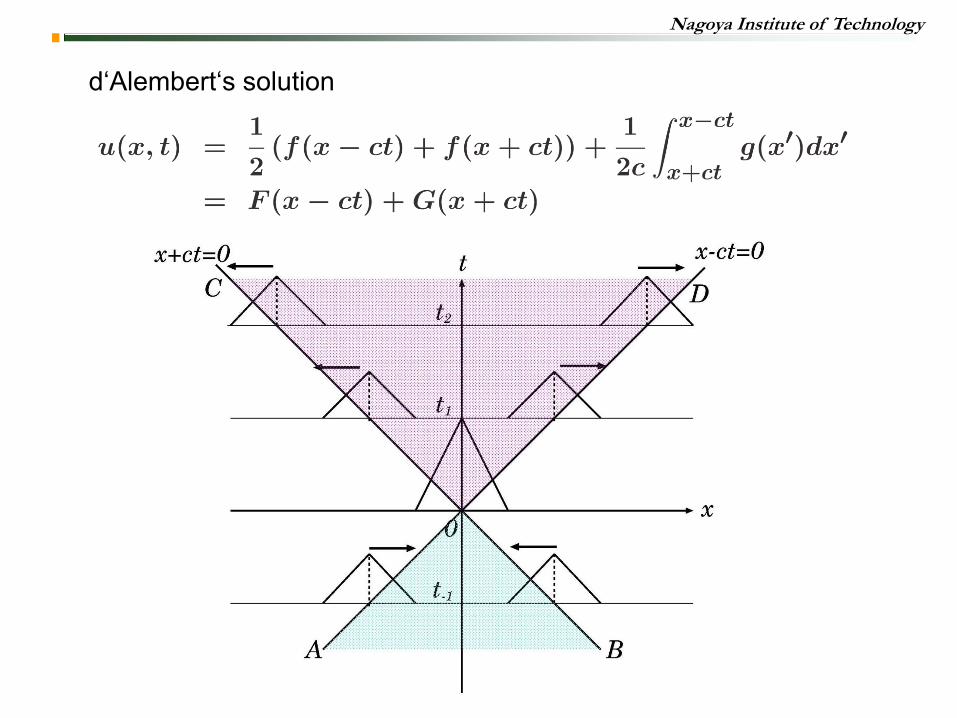
d‘Alembert‘s solution


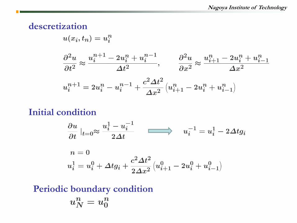
Initial condition

descretization

Periodic boundary condition


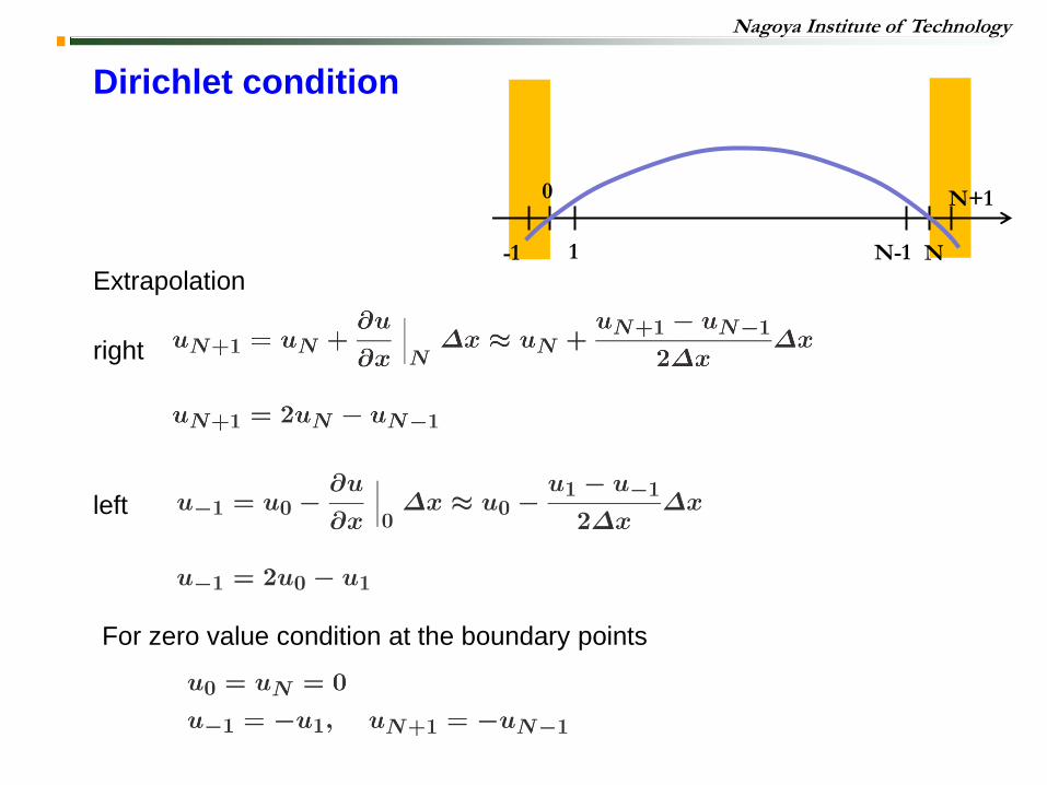
Dirichlet condition

1

0

-1 N-1 N

N+1

Extrapolation

right

For zero value condition at the boundary points

left


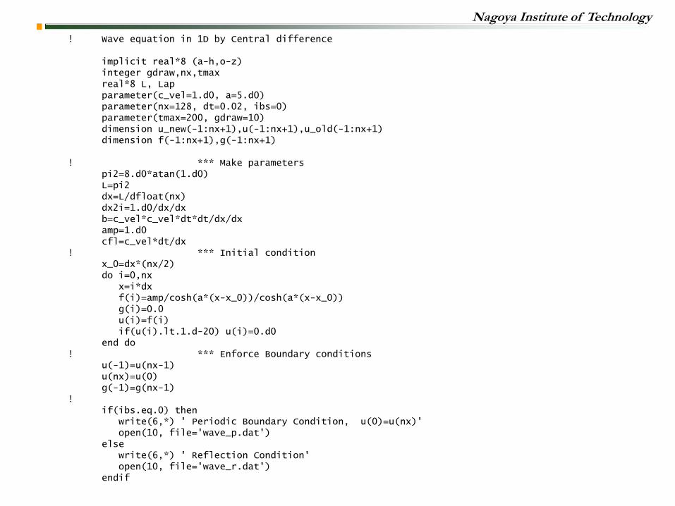
! Wave equation in 1D by Central difference implicit real*8 (a-h,o-z) integer gdraw,nx,tmax real*8 L, Lap parameter(c_vel=1.d0, a=5.d0) parameter(nx=128, dt=0.02, ibs=0) parameter(tmax=200, gdraw=10) dimension u_new(-1:nx+1),u(-1:nx+1),u_old(-1:nx+1) dimension f(-1:nx+1),g(-1:nx+1) ! *** Make parameters pi2=8.d0*atan(1.d0) L=pi2 dx=L/dfloat(nx) dx2i=1.d0/dx/dx b=c_vel*c_vel*dt*dt/dx/dx amp=1.d0 cfl=c_vel*dt/dx ! *** Initial condition x_0=dx*(nx/2) do i=0,nx x=i*dx f(i)=amp/cosh(a*(x-x_0))/cosh(a*(x-x_0)) g(i)=0.0 u(i)=f(i) if(u(i).lt.1.d-20) u(i)=0.d0 end do ! *** Enforce Boundary conditions u(-1)=u(nx-1) u(nx)=u(0) g(-1)=g(nx-1) ! if(ibs.eq.0) then write(6,*) ' Periodic Boundary Condition, u(0)=u(nx)' open(10, file='wave_p.dat') else write(6,*) ' Reflection Condition' open(10, file='wave_r.dat') endif


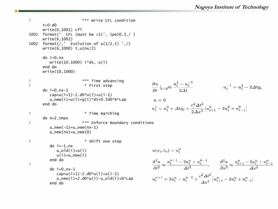
! *** Write CFL condition t=0.d0 write(6,1001) cfl 1001 format(' CFL (must be <1)', 1pe10.3,/ ) write(6,1002) 1002 format(/,' Evolution of u(1/2,t) ',/) write(6,1000) t,u(nx/2) do i=0,nx write(10,1000) i*dx, u(i) end do write(10,1000) ! *** Time advancing ! * First step do i=0,nx-1 Lap=u(i+1)-2.d0*u(i)+u(i-1) u_new(i)=u(i)+g(i)*dt+0.5d0*b*Lap end do ! * Time marching do n=2,tmax ! *** Enforce Boundary conditions u_new(-1)=u_new(nx-1) u_new(nx)=u_new(0) ! * Shift one step do i=-1,nx u_old(i)=u(i) u(i)=u_new(i) end do ! do i=0,nx-1 Lap=u(i+1)-2.d0*u(i)+u(i-1) u_new(i)=2.d0*u(i)-u_old(i)+b*Lap end do


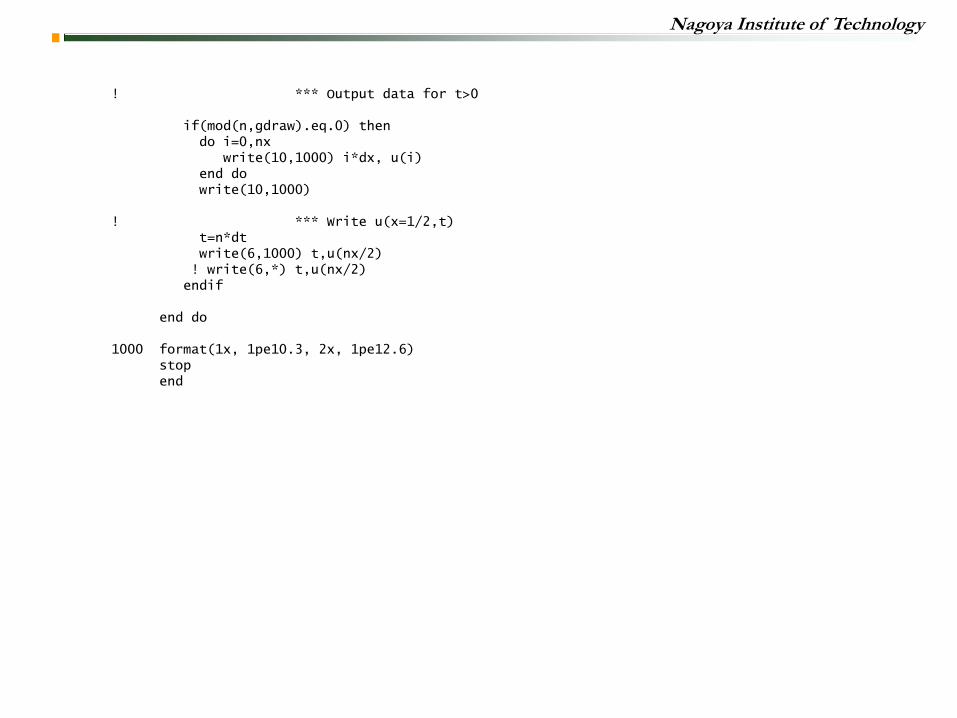
! *** Output data for t>0 if(mod(n,gdraw).eq.0) then do i=0,nx write(10,1000) i*dx, u(i) end do write(10,1000) ! *** Write u(x=1/2,t) t=n*dt write(6,1000) t,u(nx/2) ! write(6,*) t,u(nx/2) endif end do 1000 format(1x, 1pe10.3, 2x, 1pe12.6) stop end



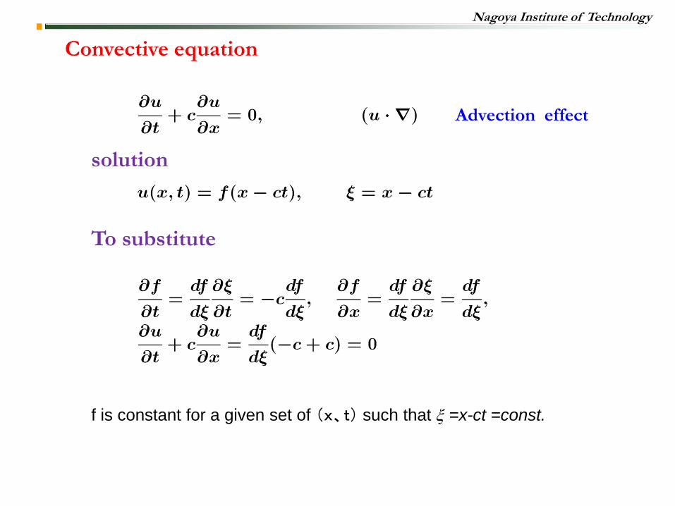
Convective equation

solution

To substitute

Advection effect

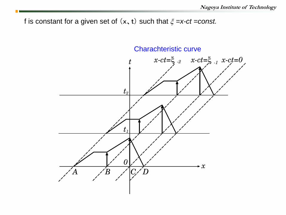
f is constant for a given set of （ｘ、ｔ） such that x =x-ct =const.


Charachteristic curve

f is constant for a given set of （ｘ、ｔ） such that x =x-ct =const.


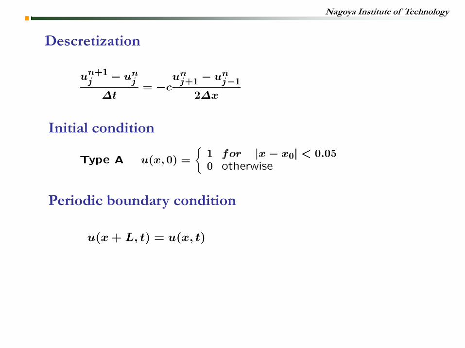
Initial condition

Descretization

Periodic boundary condition


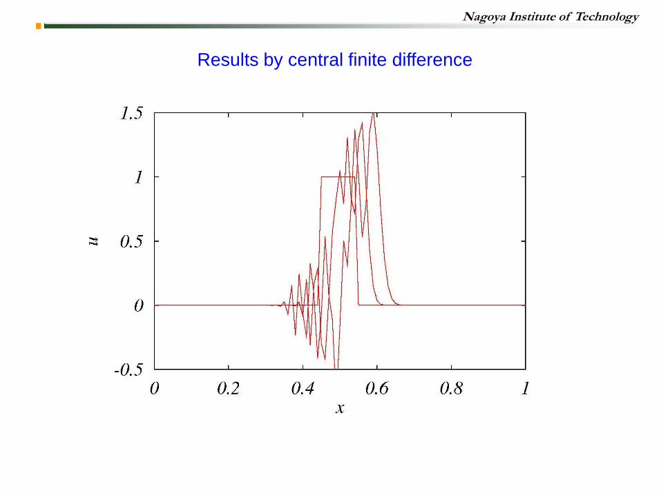
Results by central finite difference


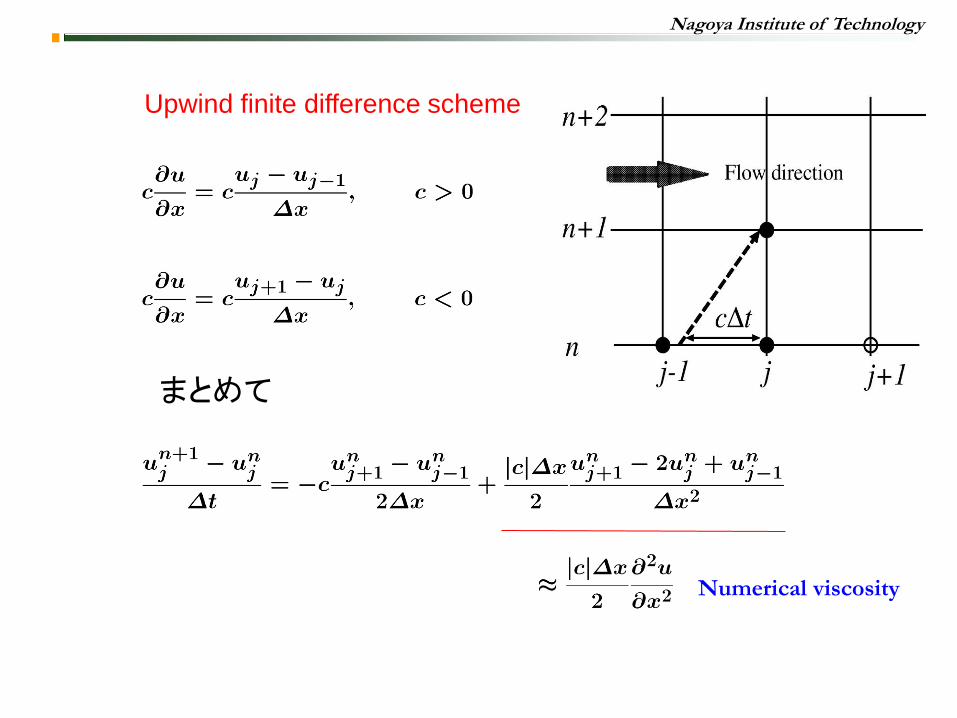
Upwind finite difference scheme

まとめて

Numerical viscosity


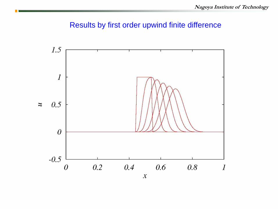
Results by first order upwind finite difference


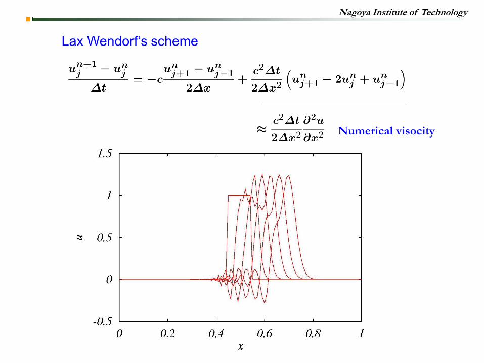
Lax Wendorf‘s scheme

Numerical visocity


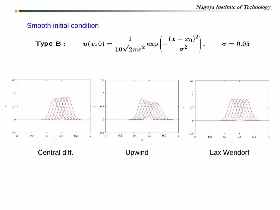
Central diff. Lax Wendorf Upwind

Smooth initial condition


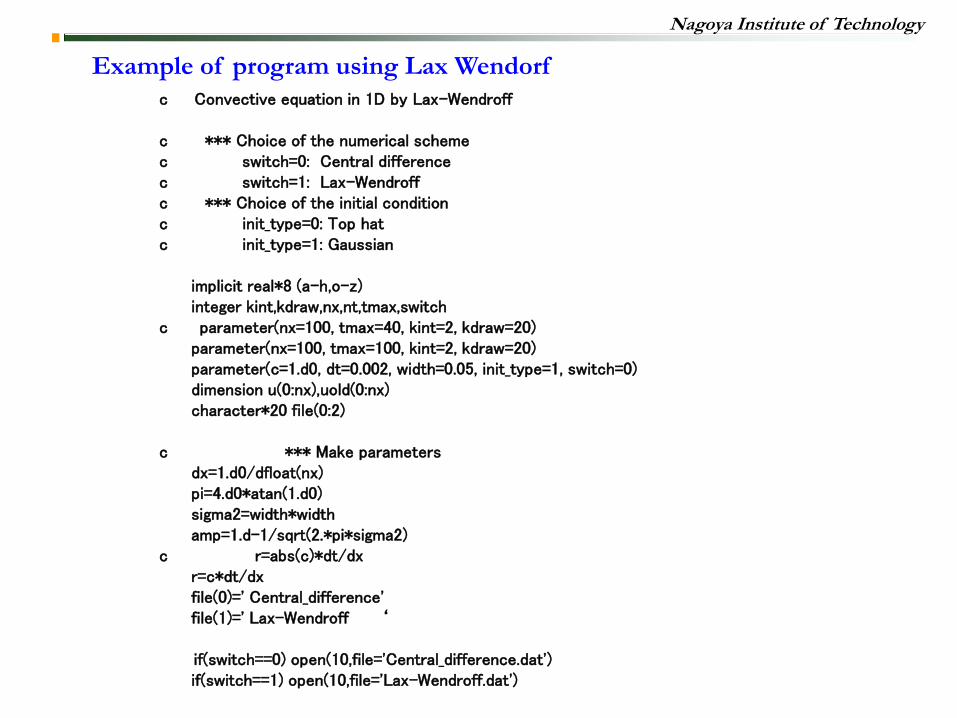
c Convective equation in 1D by Lax-Wendroff c *** Choice of the numerical scheme c switch=0: Central difference c switch=1: Lax-Wendroff c *** Choice of the initial condition c init_type=0: Top hat c init_type=1: Gaussian implicit real*8 (a-h,o-z) integer kint,kdraw,nx,nt,tmax,switch c parameter(nx=100, tmax=40, kint=2, kdraw=20) parameter(nx=100, tmax=100, kint=2, kdraw=20) parameter(c=1.d0, dt=0.002, width=0.05, init_type=1, switch=0) dimension u(0:nx),uold(0:nx) character*20 file(0:2) c *** Make parameters dx=1.d0/dfloat(nx) pi=4.d0*atan(1.d0) sigma2=width*width amp=1.d-1/sqrt(2.*pi*sigma2) c r=abs(c)*dt/dx r=c*dt/dx file(0)=' Central_difference' file(1)=' Lax-Wendroff ‘ if(switch==0) open(10,file='Central_difference.dat') if(switch==1) open(10,file='Lax-Wendroff.dat')

Example of program using Lax Wendorf


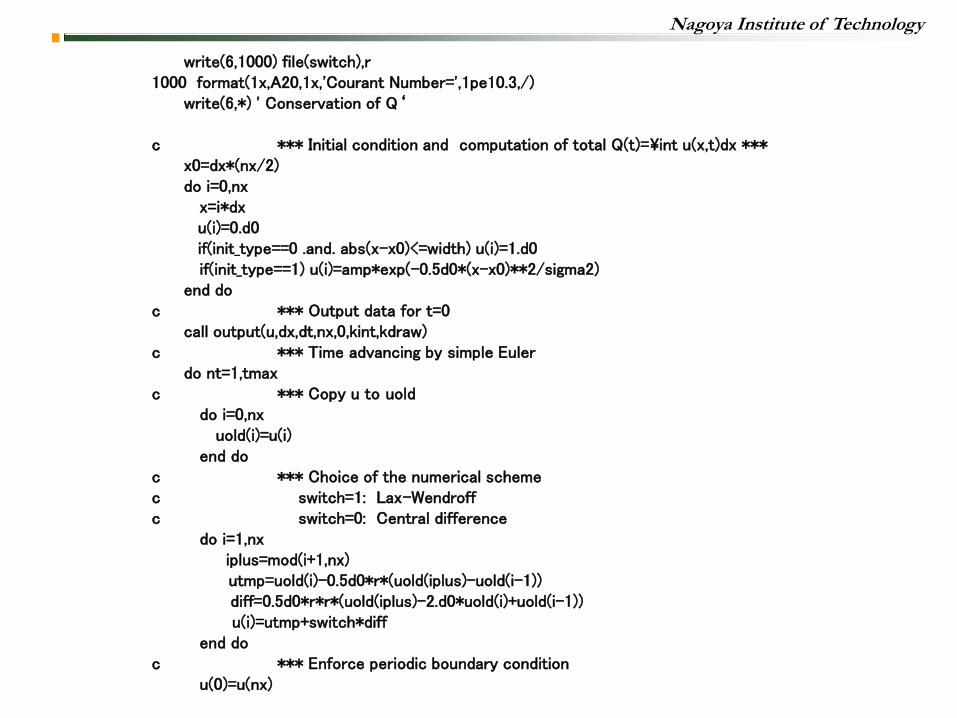
write(6,1000) file(switch),r 1000 format(1x,A20,1x,'Courant Number=',1pe10.3,/) write(6,*) ' Conservation of Q‘ c *** Initial condition and computation of total Q(t)=\int u(x,t)dx *** x0=dx*(nx/2) do i=0,nx x=i*dx u(i)=0.d0 if(init_type==0 .and. abs(x-x0)<=width) u(i)=1.d0 if(init_type==1) u(i)=amp*exp(-0.5d0*(x-x0)**2/sigma2) end do c *** Output data for t=0 call output(u,dx,dt,nx,0,kint,kdraw) c *** Time advancing by simple Euler do nt=1,tmax c *** Copy u to uold do i=0,nx uold(i)=u(i) end do c *** Choice of the numerical scheme c switch=1: Lax-Wendroff c switch=0: Central difference do i=1,nx iplus=mod(i+1,nx) utmp=uold(i)-0.5d0*r*(uold(iplus)-uold(i-1)) diff=0.5d0*r*r*(uold(iplus)-2.d0*uold(i)+uold(i-1)) u(i)=utmp+switch*diff end do c *** Enforce periodic boundary condition u(0)=u(nx)


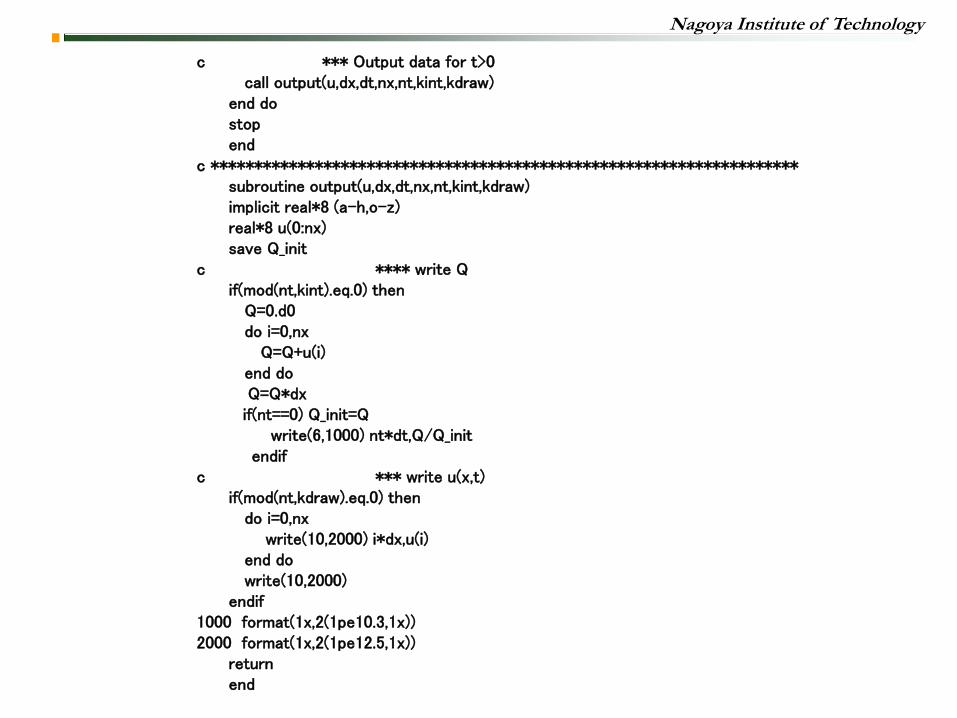
c *** Output data for t>0 call output(u,dx,dt,nx,nt,kint,kdraw) end do stop end c ******************************************************************** subroutine output(u,dx,dt,nx,nt,kint,kdraw) implicit real*8 (a-h,o-z) real*8 u(0:nx) save Q_init c **** write Q if(mod(nt,kint).eq.0) then Q=0.d0 do i=0,nx Q=Q+u(i) end do Q=Q*dx if(nt==0) Q_init=Q write(6,1000) nt*dt,Q/Q_init endif c *** write u(x,t) if(mod(nt,kdraw).eq.0) then do i=0,nx write(10,2000) i*dx,u(i) end do write(10,2000) endif 1000 format(1x,2(1pe10.3,1x)) 2000 format(1x,2(1pe12.5,1x)) return end


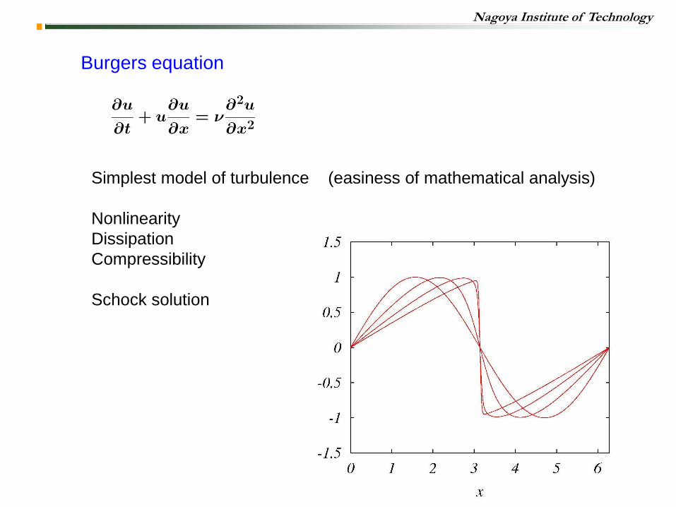
Burgers equation

Simplest model of turbulence (easiness of mathematical analysis)

Nonlinearity

Dissipation

Compressibility

Schock solution


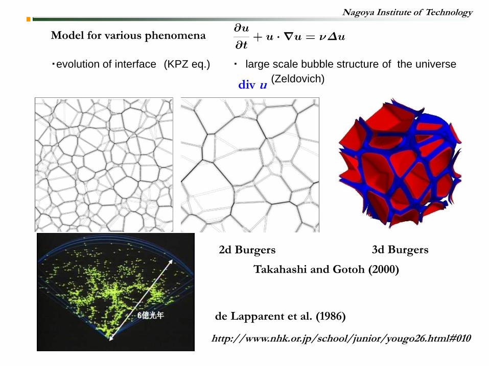
Model for various phenomena

・evolution of interface (KPZ eq.) ・ large scale bubble structure of the universe

(Zeldovich)

http://www.nhk.or.jp/school/junior/yougo26.html#010

de Lapparent et al. (1986)

2d Burgers 3d Burgers

Takahashi and Gotoh (2000)

div u


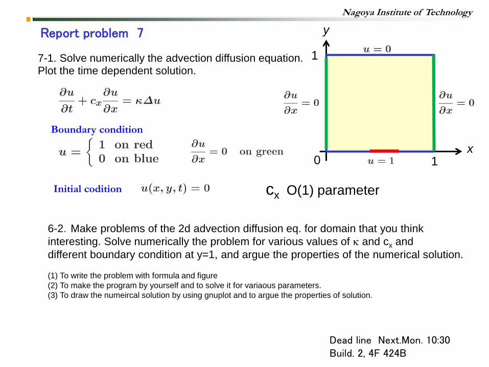
Report problem 7

Boundary condition

Initial codition

1

1 0

y

x

7-1. Solve numerically the advection diffusion equation. Plot the time dependent solution.

Dead line Next.Mon. 10:30 Build. 2, 4F 424B

6-2．Make problems of the 2d advection diffusion eq. for domain that you think

interesting. Solve numerically the problem for various values of k and cx and

different boundary condition at y=1, and argue the properties of the numerical solution.

(1) To write the problem with formula and figure

(2) To make the program by yourself and to solve it for variaous parameters.

(3) To draw the numeircal solution by using gnuplot and to argue the properties of solution.

cx O(1) parameter

Documents

Numerical computation of partial differential equation 2fluid.web.nitech.ac.jp/Gotoh_Home_page/Edu/Under_Graduate_course/... · Numerical computation of partial differential equation