MATHICSE

Mathematics Institute of Computational Science and Engineering

School of Basic Sciences - Section of Mathematics

Address:

EPFL - SB - MATHICSE (Bâtiment MA)

Station 8 - CH-1015 - Lausanne - Switzerland

http://mathicse.epfl.ch

Phone: +41 21 69 37648

Fax: +41 21 69 32545

Numerical methods for stochastic

partial differential equations

with multiple scales

Assyr Abdulle, G. A. Pavliotis

MATHICSE Technical Report Nr. 20.2011

May 2011

Numerical methods for stochastic partial differential

equations with multiple scales

A. Abdulle

Mathematics Section, Ecole Polytechnique Federale de Lausanne, CH-1015 Lausanne,

Switzerland

G.A. Pavliotis

Department of Mathematics, Imperial College London, London SW7 2AZ, UK

Abstract

A new method for solving numerically stochastic partial differential equa-tions (SPDEs) with multiple scales is presented. The method combinesa spectral method with the heterogeneous multiscale method (HMM) pre-sented in [W. E, D. Liu, and E. Vanden-Eijnden, Comm. Pure Appl. Math.,58(11):1544–1585, 2005]. The class of problems that we consider are SPDEswith quadratic nonlinearities that were studied in [D. Blomker, M. Hairer,and G. A. Pavliotis, Nonlinearity, 20(7):1721–1744, 2007.] For such SPDEsan amplitude equation which describes the effective dynamics at long timescales can be rigorously derived for both advective and diffusive time scales.Our method, based on micro and macro solvers, allows to capture numeri-cally the amplitude equation accurately at a cost independent of the smallscales in the problem. Numerical experiments illustrate the behavior of theproposed method.

Keywords: Stochastic Partial Differential Equations; Multiscale Methods;Averaging; Homogenization; Heterogeneous Multiscale Method (HMM)

1. Introduction

Many interesting phenomena in the physical sciences and in applicationsare characterized by their high dimensionality and the presence of many dif-ferent spatial and temporal scales. Standard examples include atmosphereand ocean sciences [1], molecular dynamics [2] and materials science [3]. The

mathematical description of phenomena of this type quite often leads to infi-nite dimensional multiscale systems that are described by nonlinear evolutionpartial differential equations (PDEs) with multiple scales.

Often physical systems are also subject to noise. This noise might beeither due to thermal fluctuations [4], noise in some control parameter [5],coarse-graining of a high-dimensional deterministic system with random ini-tial conditions [6, 7], or the stochastic parameterization of small scales [8].High dimensional multiscale dynamical systems that are subject to noise canbe modeled accurately using stochastic partial differential equations (SPDEs)with a multiscale structure. As examples of mathematical modeling usingSPDEs we mention the stochastic Navier-Stokes equations [9] that arise inthe study of hydrodynamic fluctuations, the stochastic Swift-Hohenberg andstochastic Kuramoto-Shivashinsky equation that arise in the study of pat-tern formation [10], the Langevin-type SPDEs that arise in path samplingand Markov Chain Monte Carlo in infinite dimensional dimensions [11] andthe stochastic KPZ equation that is used in the modeling of the evolutionof growing interfaces. Most of the equations mentioned above are semilin-ear parabolic equations with quadratic nonlinearities for which the numericalalgorithm proposed in this paper can be applied, in principle.

There are very few instances where SPDEs with multiple scales can betreated analytically. The goal of this paper is to develop numerical meth-ods for solving accurately and efficiently multiscale SPDEs. Several numer-ical methods for SPDEs have been developed and analyzed in recent years,e.g. [12, 13, 14], based on a finite difference scheme in both space and time.It is well known that explicit time discretization via standard methods (e.g.,as the Euler-Maruyama method) leads to a time-step restriction due to thestiffness originating from the discretisation of the diffusion operator (e.g. theCourant-Friedrichs-Lewy (CFL) condition ∆t ≤ C(∆x)2, where ∆t and ∆xare the time and space discretization, respectively). The situation is evenworse for SPDEs with multiple scales (e.g. of the form (3) and (4) below) asin this case the CFL condition becomes ∆t ≤ C(∆x · ε)2, where ε� 1 is theparameter measuring scale separation. Standard explicit methods becomeuseless for SPDEs with multiple scales.

Such time-step restriction can in theory be removed by using implicitmethods as was shown in [14]. However the implicitness of the numericalscheme forces one to solve potentially large linear algebraic problems at eachtime step. Furthermore, it was shown in [15] that implicit methods are notsuited for studying the long time dynamics of fast-slow stochastic systems as

2

they do not capture the correct invariant measure of the system. Althoughthis result has been obtained for finite dimensional stochastic systems, itis expected that it also applies to infinite dimensional fast-slow systems ofstochastic differential equations (SDEs), rendering the applicability of im-plicit methods to SPDEs with multiple scales questionable. We also notethat a new class of explicit methods, the S-ROCK methods, with much bet-ter stability properties than the Euler-Maruyama method was recently intro-duced in [16, 17, 18]. Although these methods are much more efficient thantraditional explicit methods, computing time issues will occur when tryingto solve SPDEs with multiple scales as considered here, since the stiffnessis extremely severe for small ε. Furthermore, capturing the correct invariantmeasure of the SPDE for ∆t > ε is still an issue for such solvers.

In this paper we consider SPDEs of the form

∂tv = Av + F (v) + εQξ, (1)

posed in a bounded domain of R with appropriate boundary conditions. Thedifferential operator A is assumed to be a non-positive self-adjoint operatorin a Hilbert space H with compact resolvent, ξ denotes space-time Gaussianwhite noise, Q is the covariance operator of the noise and we take ε � 1.We assume that the operator A and the covariance operator of the noise Qcommute, and that A has a finite dimensional kernel. 1

The finite dimensional kernel of the operator A leads to scale separationbetween the slow dynamics in N and the fast dynamics in the orthogonalcomplement of the null space N⊥, where H = N ⊕N⊥. In this paper we willfurthermore assume that noise acts directly only on the orthogonal comple-ment N⊥. This assumption is consistent with the scaling of the noise in (1),i.e. that it is of O(ε), and it leads to the singularly perturbed SPDEs (3)and (4) below. When noise acts also on the slow variables, then, its ampli-tude has to be scaled differently in equation (1); in particular it has to beof O(ε2). In this case, and after rescaling in time, we end up with a non-singularly perturbed equation for which the analysis is easier. A problemof this type has been studied and the amplitude equation has been derivedin [39].

1Notice that the compactness of the resolvent of A implies that the operator has dis-crete spectrum which, together with the self-adjointness of A and the assumption that itcommutes with the covariance operator of the noise Q, allow to expand the solution of (1)in terms of the eigenfunctions of A.

3

For concreteness, we will focus on the class of SPDEs with quadraticnonlinearities that was considered in [19], and assume that

F (u) = f(u) + εαg(u), (2)

where f is a quadratic function (e.g. f(u) = B(u, u), a symmetric bilinearform), g a linear function and the exponent α is either 1 or 2.2 The choiceof α will depend on the particular scaling. In order to describe the longtimebehavior of the SPDEs we perform an advective rescaling set v(t) := εu(εt).Using the scaling properties of white noise and (2) with α = 1 we obtain thefollowing singularly perturbed SPDE

∂tu =1

εAu+ F (u) +

1√εQξ. (3)

Another scaling is of interest, namely the diffusive rescaling v(t) := εu(ε2t)which, for (2) with α = 2 leads to the SPDE

∂tu =1

ε2Au+

1

εF (u) +

1

εQξ. (4)

Alternatively, one can start with the singularly perturbed SPDEs (3) and (4)without any reference to the SPDE (1).

Singularly perturbed SPDEs with quadratic nonlinearities provide a nat-ural testbed for testing the applicability of the heterogeneous multiscalemethod to infinite dimensional stochastic systems, since a rigorous homoge-nization theory exists for this class of SPDEs [19]. Furthermore, SPDEs ofthis form arise naturally in stochastic models for climate [1] and in surfacegrowth [21, 22]. Finally, it has already been shown through rigorous analysisand numerical experiments that these systems exhibit a very rich dynam-ical behavior, such as noise-induced transitions [23] and the possibility ofstabilization of linearly unstable modes due to the interaction between theadditive noise and the scale separation [24, 20]. We believe, however, that the

2Usually the functions f and g involve derivatives of the function u. For example,for both the Burgers and the Kuramoto-Shivashinsky equation we have f(u) = u∂xu.The linear function g(u) is included to induce a linear instability to the dynamics. Inthe case of the Burgers equation we will simply take g(u) = u whereas in the case ofthe Kuramoto-Shivashinsky equation we can take g(u) = ∂4xu. Further discussion can befound in Section 4 and in [20].

4

methodology developed in this paper has a wider range of applicability andis not restricted to SPDEs with quadratic nonlinearities. Further commentsabout the class of SPDEs for which we believe that the proposed numericalmethod can be applied can be found in Section 5.

Our numerical algorithm is based on a combination of a spectral methodwith micro-macro time integration schemes. We denote by x = Pcu theprojection onto N and by y = Psu, Ps = I−Pc the projection onto N⊥. Wethen rewrite (3) and (4) as fast-slow system of SDEs

x = a(x, y), (5a)

y =1

εAy + b(x, y) +

1√εQξ, (5b)

and

x =1

εa(x, y), (6a)

y =1

ε2Ay +

1

εb(x, y) +

1

εQξ, (6b)

where the functions a(x, y) and b(x, y) are the projections of F (u) onto NandN⊥. We emphasize the fact that the separation of scales between x and yis due to the fact that the linear operator A has a non-trivial null space, sinceAx is absent in equations (5a) and (6a). We remark that an O(1) nonlinearterm can be added in (6a). The fast-slow systems (5) and (6) resemblefast slow systems for SDEs [25, Ch. 10,11]. However, the fast process yis infinite dimensional and the well known averaging and homogenizationtheorems [26, 27] do not apply.

Averaging and homogenization results for SPDEs have been obtainedrecently [28, 19]. In particular, provided that the fast process y in (5) hassuitable ergodic properties, then the slow variable x converges, in the limitas ε tends to 0, to the solution of the averaged equation

x = a(x), (7)

where the averaged coefficient a is given by the average of a(x, y) with respectto the invariant measure of the (infinite dimensional) fast process y. Whenthis average vanishes (i.e. the centering condition from homogenization the-ory is satisfied) then the dynamics at the advective time scale becomes trivialand it is necessary to look at the dynamics at the diffusive time scale, equa-tions (6). It was shown in [19] that the slow variable x of this system of

5

equations, the solution of (6a), converges in the limit as ε tends to 0 to thesolution of the homogenized equation

x = a(x) + σ(x)ξ, (8)

with explicit formulas for the homogenized coefficients–see Section 3 for de-tails. For finite dimensional fast systems, the coefficients in (7) and (8) can becalculated, in principle, in terms of appropriate long-time averages–see [25]for details. The numerical method proposed in [29] and analyzed in [8],coined under the name of the Heterogeneous Multiscale Method (HMM),relies on the numerical approximation of the coefficients in (7) and (8) bysolving the original fine scale problem on time intervals of an intermediatetime scale and use that data to evolve the slow variables using either (7)or (8). In this paper we show how this methodology, when combined with aspectral method, can also be applied to SPDEs with multiple scales, that is,to the systems (5) and (6). The aim of the present paper is to present thealgorithm and report numerical experiments. The analysis of the proposednumerical method and the extension to more general classes of SPDEs withmultiscale structure will be presented in a forthcoming paper.

The rest of the paper is organized as follows. In Section 2 we presentour new algorithm. Analytical and computational techniques for the analysisof SPDEs with multiple scales at the heart of the multiscale algorithm arepresented in 3. In Section 4 we present numerical experiments. Section 5 isreserved for conclusions and discussion on future work.

2. Numerical method

We propose a numerical algorithm to approximate numerically the so-lution of (1) based on a micro-macro algorithm, capable of capturing theeffective behavior of the SPDE. We explain the numerical algorithm for thecase of diffusive time scale (the hardest numerically) and comment on theadvective time scale later in this section.

2.1. Multiscale Algorithm

Before stating our algorithm, we first recall our main assumptions. Weconsider SPDEs (1) in a Hilbert space H with norm ‖ · ‖ and inner product〈·, ·〉. A denotes a differential operator, ξ space-time white noise and Qthe covariance operator of the noise. We assume that A is a self-adjoint

6

nonpositive operator onH with compact resolvent. We denote its eigenvaluesand (normalized) eigenfunctions by {−λk, ek}∞k=1:

−Aek = λkek, k = 1, . . . (9)

The eigenfunctions of A form an orthonormal basis in H. We assume thatA and the covariance operator of the noise Q commute. Thus, we can write,formally,

Qξ =+∞∑k=1

qkekξk(t), (10)

where {ξk(t)}+∞k=1 are independent one-dimensional white noise processes, i.e.,mean-zero Gaussian processes with 〈ξk(t)ξj(s)〉 = δkjδ(t− s), k, j = 1, 2, . . . .Here δkj and δ(t− s) are the usual Kronecker delta functions.

Furthermore, we will assume that A has a finite dimensional kernel N :={h ∈ H : Ah = 0

}, dim(N ) = N < +∞ and write H = N ⊕ N⊥. We

introduce the projection operators

Pc : H 7→ N (11a)

Ps = I − Pc : H 7→ N⊥, (11b)

and write x := Pcu, y := Psu. Finally, we will assume that noise acts onlyon N⊥, i.e. qk = 0, k = 1 . . . N .Step 1. Decomposition in a fast-slow system.Using the projection operators defined in (11a) and (11b), equation (1) canbe written as a fast-slow stochastic system

x =1

εPcF (u), (12a)

y =1

ε2Ay +

1

εPcF (u) +

1

εQξ, (12b)

where x(t) ∈ RN since dim(N ) = N. We order the pairs of eigenfuctions andeigenvalues such that the kernel N is spanned by the first N eigenfunctionsof A. We can write

x =N∑k=1

xkek and y =+∞∑

k=N+1

ykek.

7

We introduce the vectors x = (x1, . . . xN) and y = (yN+1, . . . ) containing theFourier components (with respect to the basis {ek}∞k=1) of the functions xand y. Writing F (u) = F (x,y), we further introduce

ak(x,y) := 〈F (x, y), ek〉 for 1 ≤ k ≤ N, (13)

bk(x,y) := 〈F (x, y), ek〉 for k ≥ N. (14)

Remark 2.1. As mentioned in the introduction we will often consider thecase F (u) = f(u) + ε2g(u). Then the above decomposition reads

ak(x,y) := 〈f, ek〉+ ε〈g, ek〉 = ak0(x,y) + εak1(x,y), (15)

bk(x,y) := 〈f, ek〉+ ε〈g, ek〉 = bk0(x,y) + εbk1(x,y). (16)

where we notice that for a linear function g(u) = νu we simply have ak1(x,y) =νxk, b

k1(x,y) = νyk.

Then, in view of (9) and (10) we can rewrite the system (12) in the form

xk =1

εak(x,y), k = 1, . . . N, (17a)

yk = − 1

ε2λkyk +

1

εbk(x,y) +

1

εqkξk, k = N + 1, N + 2, . . . (17b)

Equations (12), resp. (17), are the infinite system of singularly perturbedSDEs that we want to solve numerically.

Step 2. Truncation.We consider a finite dimensional truncation of the above system and keep Mfast processes 3 :

x =1

εa(x,y), (18a)

y = − 1

ε2ΛMy +

1

εb(x,y) +

1

εQMξ, (18b)

3 To simplify the notations we will use a new labeling of the index for the truncated fastsystem and write (y1, . . . , yM )instead of (yN+1, . . . , yN+M ) and similarly for the nonzeroeigenvalues λk and the nonzero noise intensity qk.

8

where x = (x1, . . . , xN)T ,y = (y1, . . . , yM)T , ξ = (ξ1, . . . , ξM)T 4 and

a(x,y) = (a1(x,y), . . . , aN(x,y))T , (19)

b(x,y) = (b1(x,y), . . . , bM(x,y))T , (20)

and ΛM = diag(λ1, . . . , λM) and QM = diag(q1, . . . , qM). For the decompo-sition (16),(15), we will use the notations

a(x,y) = a0(x,y) + εa1(x,y), (21)

b(x,y) = b0(x,y) + εb1(x,y), (22)

where a0, a1 ∈ RN and b0,b1 ∈ RM with components similar as in (19) or(20).

Step 3. Numerical solution of the reduced system.

The reduced system (18) is solved by a micro-macro algorithm following[29, 8]. It consists of a macrosolver chosen here to be the Euler-Maruyamascheme

Xn+1 = Xn + ∆tanM + σnM∆Wn, (23)

where ∆Wn (the Wiener increment) is N (0,∆t) and Xn is a numerical ap-proximation of X(tn), the solution of a homogenized problem of the type(31). Notice that ∆t represents here a macrotime step, i.e., ∆t can be chosenmuch larger than ε. The drift function anM ' aM(Xn) and diffusion functionσnM ' σM(Xn) appearing in (23), recovered from a time-ensemble average,

4For simplicity we use the same notation y for the full and truncated vector containingthe Fourier components of the fast process

9

are given by

anM =1

KL

K∑j=1

`T+L−1∑`=`T

∂ya(Xn, Y1n,`,j)Y

2n,`,j

+1

K L

δt

ε2

K∑j=1

nT+L−1∑`=`T

L′∑`′=0

∂xa(Xn, Y1n,`+`′,j)a(Xn, Y

1n,`,j),

(24a)

σnM(σnM)T =1

K L

2δt

ε2

K∑j=1

`T+L−1∑`=`T

L′∑`′=0

a(Xn, Y1n,`+`′,j)⊗ a(Xn, Y

1n,`,j),

(24b)

where Y 1, Y 2 are the solutions of a suitable auxiliary system (given in (25)below) involving the fast problem (18b). Here K denotes the number of sam-ples taken for the numerical calculation, L, L′ the number of micro timestepsand `T a number of initial micro timesteps that are omitted in the averagingprocesses to reduce the effect of transients (see below).

Auxiliary system. As observed in [29], for diffusive timescales, computingeffective coefficients via time-averaging (relying on ergodicity), may requireto solve (18b) over time T = O(ε−2). To overcome this problem, it wassuggested again in [29] to replace the fast process in (18b) by (y ' y1 + εy2)

y1 = − 1

ε2ΛMy1 +

1

εQMξ, (25a)

y2 = − 1

ε2ΛMy2 +

1

ε2b(x,y1). (25b)

The numerical approximations Y 1, Y 2 of (25a) and (25b), respectively, arethe functions appearing in the averaging procedure to recover the macro-scopic drift and diffusion functions (see (24a))-(24b)). Notice that we fix theslow variables in the system (25b) at the current macro state Xn. We useagain the Euler-Maruyama method and compute Y 1, Y 2 as

Y 1n,`+1 = Y 1

n,` −δt

ε2ΛMY

1n,` +

√δt

εQMξn, (26a)

Y 2n,`+1 = Y 2

n,` −δt

ε2ΛMY

2n,` +

δt

ε2b(Xn, Y

1n,`), (26b)

10

where ξn = diag(ξ1n, . . . , ξMn ) and ξkn is a N (0, 1) random variable. The index

n refers to the macrotime, tn. We compute (26a) over L+L′ microtime steps,(26b) over L microtime steps to compute the time-ensemble average (24a).Notice that for the microsolver, the timestep δt resolves the fine scale ε2. Theinitial values for the micro solver are taken to be (for n ≥ 1

Y 1n,0 = Y 1

n−1,`T+L+L′−1, Y 2n,0 = Y 2

n−1,`T+L−1,

and Y 10,0 = Y 2

0,0 = 0 for n = 0. The motivation for computing the above timeaverages is given in the next section.

Remark 2.2. We notice that the auxiliary system (25) is degenerate, sincethe noise in (18b) is additive.5 This implies that the results presented in [8,App. B] are not applicable in this case and a more elaborate analysis isrequired for proving geometric ergodicity. This analysis, based on the ergodictheory for hypoelliptic diffusions [30], will be presented elsewhere. In thepresent paper we will assume that the auxiliary process (25) is ergodic.

Advective time scale.. A similar algorithm can be derived for the advectivetime scale. We consider the fast-slow system (5) that after projection andtruncation reads

x = a(x,y), (27a)

y = −1

εΛMy + b(x,y) +

1√εQMξ, (27b)

similarly as (18). The macrosolver, chosen to be the Euler explicit method,is given by

Xn+1 = Xn + ∆tanM ,

where the effective force aM is given by the time average

anM =1

KL

K∑j=1

`T+L−1∑`=`T

a(Xn, Yn,`,j), (28)

(29)

5Indeed, the auxiliary system in [29, 8] will always be degenerate, whenever the noisein the fast/slow system of SDEs that we want to solve is additive.

11

where Yn,`,j is a numerical approximation of the truncated fast system (37b)with a slow variable fixed at time tn. As previously, K denotes the number ofsamples and L the number of micro timesteps and `T is the number of initialmicro timestep ommited to reduce the transient effects. For the advectivescaling, there is no need for an auxiliary problem for the micro solver [29].

3. Averaging and Homogenization for SPDEs

In this section we summarize recent results on the averaging and homog-enization for SPDEs [28, 19] that are the analytical foundation on which thenumerical algorithm presented in Section 2 is built.

3.1. Analytic form of the homogenized coefficients

In this section we briefly discuss the analytical form of the effective systemcorresponding to (18). Under the assumption that the vector field a0(x,y)(see (21)) is centered with respect to the invariant measure of the fast process,∫

RMa0(x,y)µ(dy) = 0, (30)

then the slow process converges to a homogenized equation of the form

dX = aM(X) dt+ σM(X) dW, (31)

where W represent an N−dimensional Wiener process and the SDE (31) isinterpreted in the Ito sense. The subscript M are used to emphasise the factthat the homogenized coefficients depend on the number of fast processesthat we take into account. An analytic expression for the coefficients thatappear in (31) is given by

aM(x) = limε→0

∫RM×RM

νεx(dy1, dy2)∇ya(x,y1)y2 (32a)

+ limε→0

∫RM

µ(dy1)

∫ +∞

0

Ey1∇xa(x,y1ε2s)a(x,y1) ds,

σM(x)(σM(x))T = 2 limε→0

∫RM

µ(dy1)a(x,y1)

⊗∫ +∞

0

Ey1a(x,y1ε2s)ds. (32b)

12

Here µ(dy1) denotes the invariant measure of the process y1 which is givenby (34) and νεx(dy

1, dy2) denotes the invariant measure of the the process{y1, y2}. Notice that y1

ε2s = y1τ is the solution of the rescaled process corre-

sponding to (25a), i.e., ˙y1 = −ΛM y1+QMξ. Alternatively, the calculation ofthe coefficients aM(x) and σM(x) which appear in the homogenized equationcan be obtained by the solution of the Poisson equation

−LMφ = a0(x, y), (33)

where LM is the generator of the fast (truncated) Ornstein-Uhlenbeck pro-cess. This process is ergodic and its invariant measure is Gaussian6 :

µ(dy) =1

ZMe−

∑Mj=1

λjy2j

q2j dy, (34)

where ZM denotes the normalization constant. We notice that the sys-tem (18) is a finite dimensional fast-slow system of SDEs for which stan-dard homogenization theory applies [26, 27, 25]. For quadratic nonlinearitiesthe Poisson equation (33) can be solved analytically. The calculation of thecoefficients in the homogenized (amplitude) equation reduces then to the cal-culation of Gaussian integrals that can also be done analytically. This willbe done in Section 3.3.

3.2. The Advective Time Scale

Averaging problems for fast-slow systems of SPDEs were studied recentlyin [28] and their results can be applied to (5). One important observation isthat in the system (5), the fast process is, to leading order O(1/ε), an infinitedimensional Ornstein-Uhlenbeck process. The ergodic properties of such aninfinite dimensional process can be analyzed in a quite straightforward wayand the invariant measure, if it exists, is a Gaussian measure in an appro-priate Hilbert space that can be written down explicitly [31, 32].7 Assumingthat the process

∂tz = Az +Qξ (35)

6The notation used is explained in footnote 3 ; in particular, {λj}Mj=1 and {qj}Mj=1

denotes the first M nonzero eigenvalues/noise intensities.7The analysis presented in [28] also applies to the case where the fast process is given

by a semilinear parabolic SPDE. In this more general case, however, it is not possible toobtain an explicit formula for the invariant measure of the fast process.

13

is ergodic with Gaussian invariant measure µ with mean 0 and covarianceoperator 1

2A−1Q2, µ ∼ N

(0, 1

2A−1Q2

)then the slow process x converges to

the solution of the averaged equation

x = a(x), a(x) =

∫a(x, y)µ(dy), (36)

where the integration is over an appropriate Hilbert space. See [28, Eqn.5.2] and also [31, 32] for background material on integration with respect toGaussian measures.

When F (·) in (1) is given in terms of a symmetric bilinear map, i.e.,F (v) = B(v, v) the calculation of the vector field that appears in the aver-aged equation reduces to the calculation of Gaussian integrals and can beperformed explicitly. In this case we have

PcB(x, y) := a(x, y) = D(x, x) + C(x, y) + E(y, y),

where

Dm(x, x) =N∑

k,`=1

Bk`mxkx`,

Cm(x, y) = 2N∑k=1

∞∑`=N+1

Bk`mxky`,

Em(x, y) =∞∑

k,`=N+1

Bk`myky`, m = 1, . . . N,

and where we used the notation Bk`m := 〈B(ek, e`), em〉 and N := dim(N )denotes the dimension of the null space of A. Then, the fast-slow system (5)becomes

x = D(x, x) + C(x, y) + E(y, y), (37a)

y =1

εAy + b(x, y) +

1√εQξ, (37b)

and the averaged equation for (37) reads8

x = D(x, x) + E, (38)

8Notice that, in view of the fact that the invariant measure of (35) centered and inde-pendent of x, the linear term in y averages to 0 irrespective of the form of its dependenceon x.

14

where

Em =+∞∑

k=N+1

q2k2λk

Bkkm, m = 1, . . . N.

In the case when the null space is one-dimensional, N = 1, the averagedequation becomes

x = DX2 + E, (39)

with D = B111 and Em =∑+∞

k=N+1

q2k2λkBkk1. This equation can be solved in

closed form:

x(t) =

√E

Dtan

(√EDt+ arctan

(Dx0√ED

)).

We remark that solutions to (39), depending on the choice of the initialconditions, do not necessarily exist for all times. We also remark that it isstraightforward to consider the case where there is an additional higher orderlinear term (in ε) in the equation, i.e. F (v) = B(v, v) + ενv in the unscaledequation (1). In this case the averaged equation (38) becomes

x = D(x, x) + νx+ E,

where x ∈ RN .

3.3. The Diffusive Time Scale

We consider the system (4) obtained after a diffusive time rescaling to (1).In order to describe the homogenized equation, we further assume that F (v)in (1) is of the form

F (v) = B(v, v) + ε2νv, (40)

where B(·, ·) is a symmetric bilinear map satisfying PcB(ek, ek) = 0. 9

We recall that the noise does not act directly on the slow variables,〈Qek, ek〉 = 0, k = 1 . . . N , where N is the dimension of the null space ofA. Under appropriate assumptions on the quadratic nonlinearity and on thecovariance operator of the noise, together with the assumptions on A and Qstated earlier in this section, it is possible to prove [19] that the projection

9This is essentially the centering condition from homogenization theory, see Equa-tion (30) below.

15

of the solution to (4) onto the null space of A, x := Pcu, converges weaklyto the solution of the homogenized SDE (the amplitude equation)

dX = a(X) dt+ σ(X) dW (t), X(0) = X0. (41)

where the noise is interpreted in the Ito sense and the drift a(x) given by

a(x) = A∞x−B∞(x, x, x) + νx (42)

where the linear map A∞ : N → N and the trilinear map B∞ : N 3 → Nare defined by

A∞x = 2Bc

((I ⊗s A)−1(Bs ⊗s I) + (I ⊗A−1Bs)

+2(Bc ⊗A−1)))

(x⊗ Q), (43a)

B∞ = −2Bc(x, cA−1Bs(x, x)). (43b)

In the above we used the notation Bs := PsB and Bc := PcB, whereas ⊗sstands for the symmetric tensor product10 and where we have defined

Q =∞∑

k=N+1

q2k2λk

(ek ⊗ ek

).

The quadratic form associated with the diffusion matrix σ2 is given by

〈y, σ2(x)y〉 = 4+∞∑

k=N+1

q2k〈y,Bc(ek, x)〉2 ++∞∑

k,`=N+1

q2kq2`

2λ`(λk + λ`)〈y,Bc(ek, e`)〉2.

(44)Furthermore, the fast process can be approximated by an infinite dimensionalOrnstein-Uhlenbeck process. The precise statement and proof of the aboveresults can be found in [19].

10Given a Hilbert space H we denote by H⊗sH its symmetric tensor product. Similarly,we use the notation v1 ⊗s v2 = 1

2

(v1 ⊗ v2 + v2 ⊗ v1

)for the symmetric tensor product of

two elements and (A ⊗s B)(x ⊗ y) = 12

(Ax ⊗ By + By ⊗ Ax

)for the symmetric tensor

product of two linear operators. Furthermore, we extend the bilinear form B to the tensorproduct space by B(u⊗ v) = B(u, v). More details can be found in [19, Sec. 4].

16

Remark 3.1. The assumption that the O(ε2) term in (40) is linear is neededin order to go from (1) to (4) after rescaling or, equivalently, to (6). If ourstarting point is the already rescaled SPDE (4), then we can apply the resultsfrom [19] to nonlinearities of the form F (v) = B(v, v) + ε2h(v) where h(·)is an arbitrary nonlinearity. In this case the drift term in the amplitudeequation (42) becomes

a(x) = A∞x−B∞(x, x, x) +

∫Pch(x, y)µ(dy), (45)

where µ(dy) denotes the invariant measure of the fast OU process.

When the null space of A is one dimensional and, consequently, the ho-mogenized SDE is a scalar equation, it is possible to obtain sharp errorestimates and to prove convergence in the strong topology. In this caseEquation (41) becomes

dX = a(X) dt+ σ(X) dW, X(0) = 〈u0, e1〉 , (46)

wherea(X) = A∞X −B∞X3, σ(X) =

√C∞ +D∞X2. (47)

In the one dimensional case the formulas for the coefficients that appear inthe homogenized equation have a simpler form than in the multidimensionalcase. In particular, we have, with Bk`m = 〈B(ek, e`), em〉:

A∞ = ν +∞∑k=2

2B2k11q

2k

λ2k+

∞∑k,`=2

Bk11B``kq2`

λkλ`+

∞∑k,`=2

2Bk`1Bk1`

λk + λ`

q2kλk

, (48a)

B∞ = −∞∑k=2

2Bk11B11k

λk, (48b)

C∞ =∞∑

m,k=2

2B2km1q

2kq

2m

(λk + λm)2λk, D∞ =

∞∑k=2

4B2k11q

2k

λ2k. (48c)

It is worth mentioning that if we are using a non-orthonormal basis, i.e. abasis ek = ckek, then the coefficients that appear on the right hand side ofthe above equation transform according to

Bk`m =ckc`cm

Bk`m. (49)

We also have qk = ckqk.

17

Remark 3.2. The formulas for the coefficients that appear in the amplitudeequation (41) can be also obtained by writing the SPDE (6) in Fourier space,truncating and then using singular perturbation theory-type of techniques forthe corresponding backward Kolmogorov equation [33, 34]. More details onthis approach can be found in [35]. We also remark that, in general, bothadditive as well as multiplicative noise will appear in the amplitude equation,although only (degenerate) additive noise is present on the SPDE (1).

4. Numerical Experiments

In this section we apply our numerical method to several SPDEs andreport its convergence and performance. We consider here several examplesof SPDEs with quadratic nonlinearities and check that the theory developedin [19] and summarized in Section 3 applies. For all of these examples wecan derive rigorously the homogenized equation, with explicit formulas forthe coefficients and therefore, we can present a rigorous numerical study forour algorithm and test the effectiveness of the proposed numerical algorithm.

4.1. Theoretical considerations

We will consider variants of the Burgers and the Kuramoto-Shivashinsky(KS) equations (with a linear instability term added) in one dimension witheither Dirichlet or periodic boundary conditions. In particular, we will con-sider the singularly perturbed SPDEs (i.e. we have already rescaled to thediffusive time scale)

∂tu =1

ε2(∂2x + 1)u+

1

εu∂xu+ νu+

1

εQξ (50)

and

∂tu =1

ε2(−∂2x − ∂4x)u+

1

εu∂xu+ νu+

1

εQξ, (51)

respectively, where the noise ξ is as in Section 3. The operator Q, the co-variance operator of the noise, has eigenvalues {qk}∞k=1 and eigenfunctions{ek}∞k=1, which are also the eigenfunctions of the differential operator thatappears in either (50) or (51), i.e. the two operators commute. We will con-sider these two equations either on [0, π] with Dirichlet boundary conditionsor on [−π, π] with periodic boundary conditions.

18

Remark 4.1. For the Burgers nonlinearity and for the boundary conditionsthat we consider it is straightforward to check that the centering conditionPcB(ek, ek) = 0 is satisfied. A more natural equation to consider than (51)would be the KS equation in the small viscosity regime, i.e.

∂tu =1

ε2(−∂2x − µ∂4x)u+

1

εu∂xu+

1

εQξ,

where µ = 1− ν, ν ∈ (0, 1). This equation can be rewritten in the form

∂tu =1

ε2(−∂2x − ∂4x)u+

1

εu∂xu+ ν∂4xu+

1

εQξ. (52)

The theory presented in [19] and the numerical scheme developed in this paperapply to this equation. The application of the numerical method developed inthis paper to Equation (52) and to related models will be presented elsewhere.Some recent analytical and numerical results on the behaviour of solutionsto (52) have been reported in [20].

We will use the notation

AB = (∂2x + 1) and AKS = −∂2x − ∂4x.

It is possible to check that for the above equations and for the chose boundaryconditions the theory developed in [19] and summarized in Section 3 applies.Consider first equations (50) and (51) on [0, π] with Dirichlet boundary con-ditions. In this case the null space of AB and AKS is one dimensional:

N (A∗) = span{

sin(·)}.

with ∗ being either B or KS. The normalized eigenfunctions of AB and AKSare ek =

√2π

sin(πk). The corresponding eigenvalues are

λBk = k2 − 1 and λKSk = k4 − k2, for k = 1, 2, . . ..

Since the null space is one-dimensional, the homogenized equation is a scalarSDE. For the nonlinearity B[u, v] = 1

2∂x(uv) it is straightforward to calculate

Bk`m = 〈B(ek, e`), em〉. We have

Bk`m =1

2√

2π

(|k + `|δk+`,m − |k − `|δ|k−`|,m

), (53)

19

where δk` denotes the Kronecker delta. We can then use formulas (48) to cal-culate the formulas that appear in the homogenized equation. Let {−λk}+∞k=1

of either AB or AKS with Dirichlet boundary conditions. The homogenizedequation is given by (46) that we recall here for convenience

dX = a(X) dt+ σ(X) dW, (54)

where

a(X) = A∞X −1

4λ2X3, σ(X) =

√2

(q22

8λ22X2 + C∞)

). (55)

The coefficients that appear in (55) can be computed as 11

A∞ =

(ν +

1

8

q22λ22

+1

8

+∞∑k=2

kλkq2k+1 − λk+1q

2k(k + 1)

(λk+1 + λk)λkλk+1

), (56a)

C∞ =

(1

16

+∞∑k=2

q2kq2k+1

λkλk+1(λk + λk+1)

). (56b)

In the case where only the second mode is forced with noise, q2 = σ, qM =0, M = 3, . . . then the coefficients become

A∞ = ν +1

8

σ2

λ22− 3

8

σ2

λ2(λ2 + λ3), C∞ = 0.

In this case only multiplicative noise appears in the homogenized equationand it can lead to intermittent behavior of solutions as well as noise inducedtransitions [20].

We will also consider either the Burgers or the KS equation on [−π, π]with periodic boundary conditions. In this case the null space of both ABand AKS is two-dimensional and is spanned by

N (A∗) = span {sin(·), cos(·)} ,

with ∗ being either B or KS. The homogenized equation is given by (41),where X = (X1, X2). It consists of a system of two coupled SDEs. We canuse formulas (42) and (44), together with the formula for the nonlinearityB[u, v] = 1

2∂x(u v) to calculate the coefficients that appear in the homoge-

nized equation.

11We use the non-normalized basis ek = sin(πk) and use formula (49).

20

4.2. Numerical Experiments

We shall now apply our numerical algorithm to the model problems (50),(51) described in Section 4.1. As the behavior of our algorithm is similar forthe Burgers and the Kuramoto-Shivashinsky equation we will do a thoroughnumerical study on the Burgers equation and comment on the results for theKuramoto-Shivashinsky equation.Burgers Equation. We consider equation (50) on [0, π] with homogeneousDirichlet boundary conditions. We know from Section 4.1 that, for ε suffi-ciently small, we have that

u(x, t) ≈ X(t) sin(x), (57)

where X(t) is the solution of (54). The precise statement of this resulttogether with an error estimate can be found in [19, Thm. 7.1, Thm. 7.4].The function a(X), σ(X) in (47) depends on A∞, C∞ which for the Burgersequation can be computed using formulas (56) with λk = k2 − 1. They readA∞ = 0.0026744370, C∞ = 0.0002659283 (the fast convergence of the series(56) allows to compute numerically A∞, C∞ with high precision, given hereup to ten digits). Following the algorithm described in Section (2), we lookfor a solution to (50) of the form

u(x, t) ' x(t) sin(x) +M∑k=1

yk(t) sin(kx), (58)

substitute the expansion in (50) to obtain the a fast-slow system of SDEs asdescribed in (18). Following the algorithm of Section 2 we compute numeri-cally the slow variable Xn as

Xn+1 = Xn + ∆tanM + σnM∆Wn, (59)

where anM , σnM are given by (24a) and (24b), respectively. We also consider

the truncated homogenized problem, i.e.,

dX = aM(X)dt+ σM(X)dW, (60)

where

aM(X) = AMX −1

12X3, σ(X) =

√2

(1

72X2 + CM)

), (61)

21

and where AM , CM , are obtained from (56a),(56b) with the sums truncatedat M .

For numerical comparison we also compute

Xn+1,inf = Xn,inf + ∆ta(Xn,inf) + σ(Xn,inf)∆Wn, (62)

Xn+1,hom = Xn,hom + ∆taM(Xn,hom) + σM(Xn,hom)∆Wn, (63)

the Euler-Maruyama approximation of the SDEs (54) and (60), respectively.The same Brownian path will be used in (54), (59) and (60). We emphasizethat the numerical solutions for (54) and (60) rely on analytically computedhomogenized coefficients, whereas for (59) we implement the multiscale algo-rithm of Section 2, where the coefficients anM , σ

nM are computed ”on the fly”

and rely on the microsolver (26a) and (26b). Hence no a-priori analyticalknowledge of the amplitude equation is required.

We choose the values of the various parameters entering in the averagingprocess for the computation of anM , σ

nM as suggested in [8], i.e., K = 1,

δt/ε2 = O(2−p), nT = O(1), L = O(23p), L′ = O(p ·2p). According to [8], thisguarantees (for the case of non-degenerate fast processes) that the error isbounded by 2−p. In our case with a degenerate fast process an error bound isstill to be established. Here we monitor such convergence numerically. Moreprecisely, we set nT = 16, L = 23p, L′ = p · 2p and monitor the error using

EMp =

1

N

N∑n=1

(|anM − aM(Xn,hom)|+ |σnM − σM(Xn,hom)|) (64a)

EMl,p =

1

N

N∑n=1

(|anM − a(Xn,inf)|+ |σnM − σ(Xn,hom)|) , (64b)

for various values of p, where ∆t = T/N and T represent the final time.Notice that (64a) captures the error between (60)–the homogenized solutionof the truncated system–and the numerical solution of the truncated system,while (64b), where the index l stands for limit, captures the error between thehomogenized solution of the limit problem (54) and the numerical solutionof the truncated system.

2-mode truncation. We set M = 2 in (58) and substitute the expansion

22

in (50) to obtain the following system of equations

x = νx− 1

2ε

(xy1 + y1y2

), (65a)

y1 =

(ν − 3

ε2

)y1 −

1

ε

(xy2 −

1

2x2)

+q1εξ1(t), (65b)

y3 =

(ν − 8

ε2

)y2 +

3

2ε

(xy1) +

q2εξ2(t). (65c)

The auxiliary process can be derived as explained in Section 2 and reads

y11 = − 3

ε2y11 +

q1εξ1(t), (66a)

y12 = − 8

ε2y12 +

q2εξ2(t), (66b)

y21 = − 3

ε2y21 −

1

ε2

(xy12 −

x2

2

), (66c)

y22 = − 8

ε2y12 +

3

2ε2xy11. (66d)

We apply the algorithm of Section 2 to get a numerical approximation of thehomogenised problem corresponding to (65). The final time is T = 1 andN = 10, which corresponds to macro time-step of size ∆t = 0.1. The macrosolver for the method is given by (59). As mentioned above, we compare ourresults with (62) and (63). The unknown coefficients A3, C3 in (61) can becomputed using (56a) and (56b), where the sum is truncated at M + 1 = 3and read A3 = 0.003735726834, C3 = 0.0002593873518.

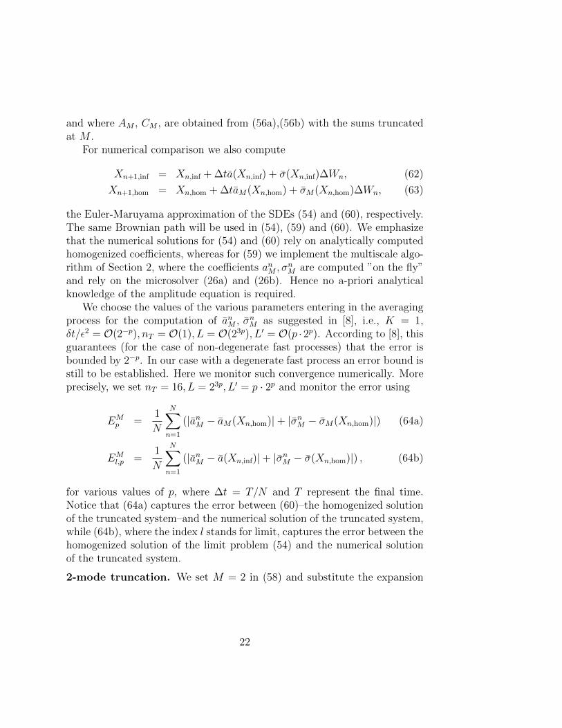
We observe in Figure 1 that we get numerically the expected order ofconvergence corresponding to δt/ε2 = O(2−p). Furthermore, as the microtime-step becomes smaller, the numerical scheme gets closer to (59) andslightly deviates from (54). This is expected as the numerical solution isnot converging to that latter solution. We observe nevertheless that withonly two fast modes, the numerical scheme already captures quite well theeffective behavior of the slow variable of the infinite dimensional system.

We also illustrate the time evolution of one trajectory comparing over thetime 0 ≤ t ≤ T with T = 10, the Euler-Maruyama method for the amplitudeequation (62), the homogenized equation (63) and the macro solver (59).The same Brownian path is used for generating the three trajectories and aswell as the same macro time step. We perform this comparison for increasing

23

3 4 5 6 710

−3

10−2

10−1

100

p

Error

2−p

Ep

2

El,p

2

Figure 1: Numerical convergence for 2-mode truncation. On the horizontal axis we monitorthe accuracy of the micro-timestep and on the vertical axis we measure the error as givenby (64a) and (64b) with M = 2.

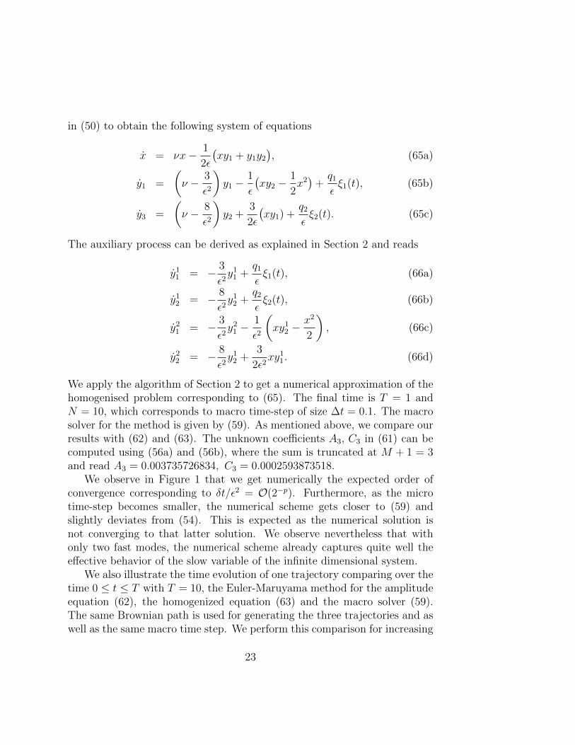
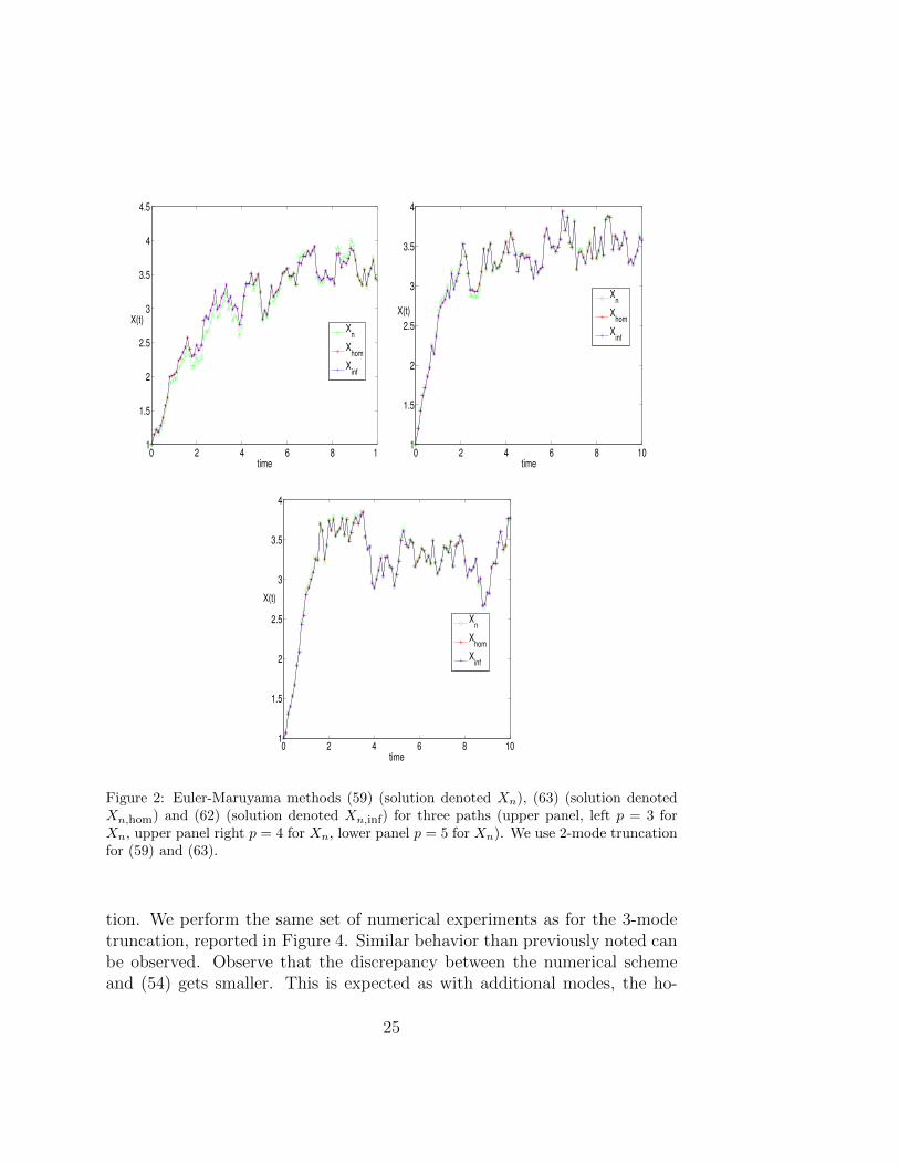
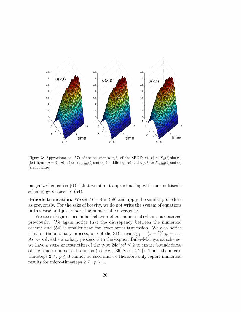
accuracy of the micro solver used to recover the macro data, namely, δt/ε2 =O(2−p), p = 3, 4, 5. We see in Figure 2 that the trajectory for the amplitudeequation and the homogenized equation coincide, while the macro solver getscloser to the true dynamics as we refine the micro time step. For the sametrajectory we also give a space-time plot for the approximation of the originalSPDE u(·, t) ≈ X(t) sin(·), with X(t) solution of the amplitude equation, thehomogenized equation or the macro solver. Again we see that the numericalmethod captures the right behavior of the solution.

3-mode truncation. We set M = 3 in (58) and obtain the following systemof equations

x = νx− 1

2ε

(xy1 + y1y2 + y2y3

), (67a)

y1 =

(ν − 3

ε2

)y1 −

1

ε

(xy2 + y1y3 −

1

2x2)

+q1εξ1(t), (67b)

y2 =

(ν − 8

ε2

)y2 −

3

2ε

(xy3 − xy1

)+q2εξ2(t), (67c)

y3 =

(ν − 15

ε2

)y3 +

1

ε

(2xy2 + y21

)+q3εξ3(t). (67d)

The auxiliary process can be computed similarly as for the 3-mode trunca-

24

0 2 4 6 8 101

1.5

2

2.5

3

3.5

4

4.5

time

X(t)

Xn

Xhom

Xinf

0 2 4 6 8 101

1.5

2

2.5

3

3.5

4

time

X(t)

Xn

Xhom

Xinf

0 2 4 6 8 101

1.5

2

2.5

3

3.5

4

time

X(t)

Xn

Xhom

Xinf

Figure 2: Euler-Maruyama methods (59) (solution denoted Xn), (63) (solution denotedXn,hom) and (62) (solution denoted Xn,inf) for three paths (upper panel, left p = 3 forXn, upper panel right p = 4 for Xn, lower panel p = 5 for Xn). We use 2-mode truncationfor (59) and (63).

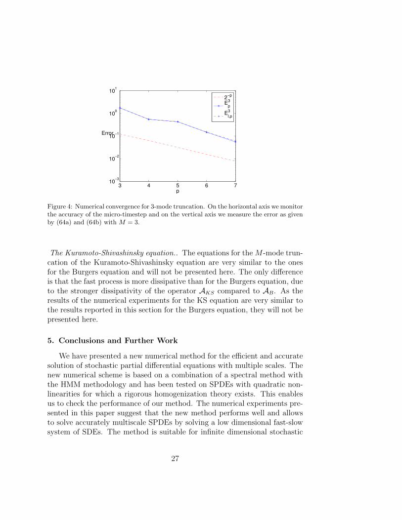
tion. We perform the same set of numerical experiments as for the 3-modetruncation, reported in Figure 4. Similar behavior than previously noted canbe observed. Observe that the discrepancy between the numerical schemeand (54) gets smaller. This is expected as with additional modes, the ho-

25

0

5

10

0

1

2

3

4

0

0.5

1

1.5

2

2.5

3

3.5

time

u(x,t)

x

0

5

10

0

1

2

3

4

0

0.5

1

1.5

2

2.5

3

3.5

time

u(x,t)

x

0

5

10

0

1

2

3

4

0

0.5

1

1.5

2

2.5

3

3.5

time

u(x,t)

x

Figure 3: Approximation (57) of the solution u(x, t) of the SPDE; u(·, t) ' Xn(t) sin(π·)(left figure p = 3), u(·, t) ' Xn,hom(t) sin(π·) (middle figure) and u(·, t) ' Xn,inf(t) sin(π·)(right figure).

mogenized equation (60) (that we aim at approximating with our multiscalescheme) gets closer to (54).

4-mode truncation. We set M = 4 in (58) and apply the similar procedureas previously. For the sake of brevity, we do not write the system of equationsin this case and just report the numerical convergence.

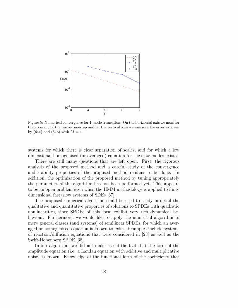
We see in Figure 5 a similar behavior of our numerical scheme as observedpreviously. We again notice that the discrepancy between the numericalscheme and (54) is smaller than for lower order truncation. We also noticethat for the auxiliary process, one of the SDE reads y4 =

(ν − 24

ε2

)y4 + . . ..

As we solve the auxiliary process with the explicit Euler-Maruyama scheme,we have a stepsize restriction of the type 24δt/ε2 ≤ 2 to ensure boundednessof the (micro) numerical solution (see e.g., [36, Sect. 4.2 ]). Thus, the micro-timesteps 2−p, p ≤ 3 cannot be used and we therefore only report numericalresults for micro-timesteps 2−p, p ≥ 4.

26

3 4 5 6 710

−3

10−2

10−1

100

101

p

Error

2−p

Ep

3

El,p

3

Figure 4: Numerical convergence for 3-mode truncation. On the horizontal axis we monitorthe accuracy of the micro-timestep and on the vertical axis we measure the error as givenby (64a) and (64b) with M = 3.

The Kuramoto-Shivashinsky equation.. The equations for the M -mode trun-cation of the Kuramoto-Shivashinsky equation are very similar to the onesfor the Burgers equation and will not be presented here. The only differenceis that the fast process is more dissipative than for the Burgers equation, dueto the stronger dissipativity of the operator AKS compared to AB. As theresults of the numerical experiments for the KS equation are very similar tothe results reported in this section for the Burgers equation, they will not bepresented here.

5. Conclusions and Further Work

We have presented a new numerical method for the efficient and accuratesolution of stochastic partial differential equations with multiple scales. Thenew numerical scheme is based on a combination of a spectral method withthe HMM methodology and has been tested on SPDEs with quadratic non-linearities for which a rigorous homogenization theory exists. This enablesus to check the performance of our method. The numerical experiments pre-sented in this paper suggest that the new method performs well and allowsto solve accurately multiscale SPDEs by solving a low dimensional fast-slowsystem of SDEs. The method is suitable for infinite dimensional stochastic

27

3 4 5 6 710

−3

10−2

10−1

100

p

Error

2−p

Ep

4

El,p

4

Figure 5: Numerical convergence for 4-mode truncation. On the horizontal axis we monitorthe accuracy of the micro-timestep and on the vertical axis we measure the error as givenby (64a) and (64b) with M = 4.

systems for which there is clear separation of scales, and for which a lowdimensional homogenised (or averaged) equation for the slow modes exists.

There are still many questions that are left open. First, the rigorousanalysis of the proposed method and a careful study of the convergenceand stability properties of the proposed method remains to be done. Inaddition, the optimisation of the proposed method by tuning appropriatelythe parameters of the algorithm has not been performed yet. This appearsto be an open problem even when the HMM methodology is applied to finitedimensional fast/slow systems of SDEs [37].

The proposed numerical algorithm could be used to study in detail thequalitative and quantitative properties of solutions to SPDEs with quadraticnonlinearities, since SPDEs of this form exhibit very rich dynamical be-haviour. Furthermore, we would like to apply the numerical algorithm tomore general classes (and systems) of semilinear SPDEs, for which an aver-aged or homogenised equation is known to exist. Examples include systemsof reaction/diffusion equations that were considered in [28] as well as theSwift-Hohenberg SPDE [38].

In our algorithm, we did not make use of the fact that the form of theamplitude equation (i.e. a Landau equation with additive and multiplicativenoise) is known. Knowledge of the functional form of the coefficients that

28

appear in the homogenised or averaged equation can be used in order tosimplify the numerical algorithm. The stochastic Landau equation appears asthe amplitude equation for several infinite dimensional stochastic dynamicalsystems, not only for SPDEs with quadratic nonlinearities, e.g. [39]. Thus,the algorithm proposed in this paper, could be modified to develop an efficientmethod for studying the dynamics of SPDEs near bifurcation. All thesetopics are currently under investigation.

Acknowledgments. Part of this work was done while GP was visiting theMathematics Section of EPFL. The hospitality of the department and ofthe group of A. Abdulle is greatly acknowledged. The authors thank S.Krumscheid for an extremely careful reading of an earlier version of thepaper and for many useful remarks. GP is supported by the EPSRC.

References

[1] A. J. Majda, C. Franzke, B. Khouider, An applied mathematics per-spective on stochastic modelling for climate, Philos. Trans. R. Soc.Lond. Ser. A Math. Phys. Eng. Sci. 366 (1875) (2008) 2429–2455.doi:10.1098/rsta.2008.0012.URL http://dx.doi.org/10.1098/rsta.2008.0012

[2] M. Griebel, S. Knapek, G. Zumbusch, Numerical simulation in moleculardynamics, Vol. 5 of Texts in Computational Science and Engineering,Springer, Berlin, 2007, numerics, algorithms, parallelization, applica-tions.

[3] J. Fish, Multiscale Methods: Bridging The Scales In Science And Engi-neering, Oxford University Press, Oxford, 2009.

[4] A. Einstein, Investigations on the theory of the Brownian movement,Dover Publications Inc., New York, 1956, edited with notes by R. Furth,Translated by A. D. Cowper.

[5] W. Horsthemke, R. Lefever, Noise-induced transitions, Vol. 15 ofSpringer Series in Synergetics, Springer-Verlag, Berlin, 1984, theory andapplications in physics, chemistry, and biology.

[6] R. Mazo, Brownian motion, Vol. 112 of International Series of Mono-graphs on Physics, Oxford University Press, New York, 2002.

29

[7] R. Zwanzig, Nonequilibrium statistical mechanics, Oxford UniversityPress, New York, 2001.

[8] W. E, D. Liu, E. Vanden-Eijnden, Analysis of multiscale methodsfor stochastic differential equations, Comm. Pure Appl. Math. 58 (11)(2005) 1544–1585.

[9] L. D. Landau, E. M. Lifshitz, Fluid mechanics, Translated from theRussian by J. B. Sykes and W. H. Reid. Course of Theoretical Physics,Vol. 6, Pergamon Press, London, 1959.

[10] M. C. Cross, P. C. Hohenberg, Pattern formation outside of equilibrium,Rev. Mod. Phys. 65 (1993) 851–1112. doi:10.1103/RevModPhys.65.851.URL http://link.aps.org/doi/10.1103/RevModPhys.65.851

[11] M. Hairer, A. M. Stuart, J. Voss, Analysis of SPDEs arising in pathsampling. II. The nonlinear case, Ann. Appl. Probab. 17 (5-6) (2007)1657–1706. doi:10.1214/07-AAP441.URL http://dx.doi.org/10.1214/07-AAP441

[12] A. Alabert, I. Gyongy, On numerical approximation of stochastic Burg-ers’ equation, in: From stochastic calculus to mathematical finance,Springer, Berlin, 2006, pp. 1–15.

[13] A. M. Davie, J. G. Gaines, Convergence of numerical schemes for the so-lution of parabolic stochastic partial differential equations, Math. Comp.70 (233) (2001) 121–134 (electronic).

[14] J. Printems, On the discretization in time of parabolic stochastic partialdifferential equations, M2AN Math. Model. Numer. Anal. 35 (6) (2001)1055–1078.

[15] T. Li, A. Abdulle, W. E, Effectiveness of implicit methods for stiffstochastic differential equations, Commun. Comput. Phys. 3 (2) (2008)295–307.

[16] A. Abdulle, S. Cirilli, Stabilized methods for stiff stochastic sys-tems, C. R. Math. Acad. Sci. Paris 345 (10) (2007) 593–598.doi:10.1016/j.crma.2007.10.009.URL http://dx.doi.org/10.1016/j.crma.2007.10.009

30

[17] A. Abdulle, S. Cirilli, S-ROCK: Chebyshev methods for stiff stochasticdifferential equations, SIAM J. Sci. Comput. 30 (2) (2008) 997–1014.doi:10.1137/070679375.URL http://dx.doi.org/10.1137/070679375

[18] A. Abdulle, T. Li, S-ROCK methods for stiff Ito SDEs, Commun.Math. Sci. 6 (4) (2008) 845–868.URL http://projecteuclid.org/getRecord?id=euclid.cms/1229619673

[19] D. Blomker, M. Hairer, G. A. Pavliotis, Multiscale analysis for stochasticpartial differential equations with quadratic nonlinearities, Nonlinearity20 (7) (2007) 1721–1744.

[20] M. Pradas, D. Tseluiko, S. Kalliadasis, D. T. Papageorgiou, G. A. Pavli-otis, Noise induced state transitions, intermittency, and universalityin the noisy kuramoto-sivashinksy equation, Phys. Rev. Lett. 106 (6)(2011) 060602. doi:10.1103/PhysRevLett.106.060602.

[21] M. Kardar, G. Parisi, Y.-C. Zhang, Dynamic scaling ofgrowing interfaces, Phys. Rev. Lett. 56 (9) (1986) 889–892.doi:10.1103/PhysRevLett.56.889.

[22] S. Zaleski, A stochastic model for the large scale dynamics of somefluctuating interfaces, Phys. D 34 (3) (1989) 427–438. doi:10.1016/0167-2789(89)90266-2.URL http://dx.doi.org/10.1016/0167-2789(89)90266-2

[23] X. Wan, X. Zhou, W. E, Study of the noise-induced transition and theexploration of the phase space for the Kuramoto-Sivashinsky equationusing the minimum action method, Nonlinearity 23 (3) (2010) 475–493.doi:10.1088/0951-7715/23/3/002.URL http://dx.doi.org/10.1088/0951-7715/23/3/002

[24] D. Blomker, M. Hairer, G. Pavliotis, Some remarks on stabilization byadditive noise, Preprint.

[25] G. Pavliotis, A. Stuart, Multiscale methods, Vol. 53 of Texts in AppliedMathematics, Springer, New York, 2008, averaging and homogenization.

31

[26] A. Bensoussan, J.-L. Lions, G. Papanicolaou, Asymptotic analysis forperiodic structures, Vol. 5 of Studies in Mathematics and its Applica-tions, North-Holland Publishing Co., Amsterdam, 1978.

[27] G. C. Papanicolaou, D. Stroock, S. R. S. Varadhan, Martingale ap-proach to some limit theorems, in: Papers from the Duke TurbulenceConference (Duke Univ., Durham, N.C., 1976), Paper No. 6, Duke Univ.,Durham, N.C., 1977, pp. ii+120 pp. Duke Univ. Math. Ser., Vol. III.

[28] S. Cerrai, M. Freidlin, Averaging principle for a class of stochasticreaction-diffusion equations, Probab. Theory Related Fields 144 (1-2)(2009) 137–177.

[29] E. Vanden-Eijnden, Numerical techniques for multi-scale dynamical sys-tems with stochastic effects, Commun. Math. Sci. 1 (2) (2003) 385–391.

[30] J. Mattingly, A. M. Stuart, Geometric ergodicity of some hypo-ellipticdiffusions for particle motions, Markov Processes and Related Fields8 (2) (2002) 199–214.

[31] G. D. Prato, J. Zabczyk, Stochastic equations in infinite dimensions,Vol. 44 of Encyclopedia of Mathematics and its Applications, CambridgeUniversity Press, Cambridge, 1992.

[32] G. Da Prato, J. Zabczyk, Ergodicity for infinite-dimensionalsystems, Vol. 229 of London Mathematical Society LectureNote Series, Cambridge University Press, Cambridge, 1996.doi:10.1017/CBO9780511662829.URL http://dx.doi.org/10.1017/CBO9780511662829

[33] T. Kurtz, A limit theorem for perturbed operator semigroups with ap-plications to random evolutions, J. Functional Analysis 12 (1973) 55–67.

[34] G. C. Papanicolaou, Some probabilistic problems and methods in sin-gular perturbations, Rocky Mountain J. Math. 6 (4) (1976) 653–674.

[35] A. Majda, I. Timofeyev, E. V. Eijnden, A mathematical framework forstochastic climate models, Comm. Pure Appl. Math. 54 (8) (2001) 891–974.

32

[36] E. Hairer and G. Wanner, Solving ordinary differential equations II. Stiffand differential-algebraic problems. Second edition, Springer-Verlag,1996.

[37] D. Liu, Optimal error estimates for heterogeneous multiscale methodsfor stochastic dynamical systems, Preprint.

[38] D. Blomker, M. Hairer, G. A. Pavliotis, Modulation equations: Stochas-tic bifurcation in large domains, Comm. Math. Phys. 258 (1) (2005)479–512.

[39] D. Blomker, S. Maier-Paape, G. Schneider, The stochastic Landau equa-tion as an amplitude equation, Discrete Contin. Dyn. Syst. Ser. B 1 (4)(2001) 527–541. doi:10.3934/dcdsb.2001.1.527.URL http://dx.doi.org/10.3934/dcdsb.2001.1.527

33