Embed Size (px)
Citation preview
9 Numerical Solution of Partial Differential Equations
9.0 Classification of Partial Differential Equations
We now consider general second-order partial differential equations (PDEs) of the form
Lu = autt + buxt + cuxx + f = 0, (1)
where u is an unknown function of x and t, and a, b, c, and f are given functions. Ifthese functions depend only on x and t, then the PDE (1) is called linear. If a, b, c, orf depend also on u, ux, or ut, then the PDE is called quasi-linear.
Remarks:
1. The notation used in (1) suggests that we think of one of the variables, t, as time,and the other, x, as space.
2. In principle, we could also have second-order PDEs involving more than one spacedimension. However, we limit the discussion here to PDEs with a total of twoindependent variables.
3. Of course, a second-order PDE can also be independent of time, and contain twospace variables only (such as Laplace’s equation).
There are three fundamentally different types of second-order quasi-linear PDEs:
• If b2 − 4ac > 0, then L is hyperbolic.
• If b2 − 4ac = 0, then L is parabolic.
• If b2 − 4ac < 0, then L is elliptic.
Examples:
1. The wave equationutt = α2uxx + f(x, t)
is a second-order linear hyperbolic PDE since a ≡ 1, b ≡ 0, and c ≡ −α2, so that
b2 − 4ac = 4α2 > 0.
2. The heat or diffusion equationut = kuxx
is a second-order quasi-linear parabolic PDE since a = b ≡ 0, and c ≡ −k, sothat
b2 − 4ac = 0.
3. Poisson’s equation (or Laplace’s equation in case f ≡ 0)
uxx + uyy = f(x, y)
is a second-order linear elliptic PDE since a = c ≡ 1 and b ≡ 0, so that
b2 − 4ac = −4 < 0.
Remarks: Since a, b, and c may depend on x, t, u, ux, and ut the classification of thePDE may even vary from point to point.
1
9.1 Forward Differences for Parabolic PDEs
We consider the following model problem
uxx = ut, t ≥ 0, 0 ≤ x ≤ 1,u(x, 0) = g(x), 0 ≤ x ≤ 1,u(0, t) = α(t), t ≥ 0,u(1, t) = β(t), t ≥ 0, (2)
which can be interpreted as the model for heat conduction in a one-dimensional rodof length 1 with prescribed end temperatures, α and β, and given initial temperaturedistribution g.
Finite Differences
We will proceed in a way very similar to our solution for two-point boundary valueproblems. However, now we are dealing with an initial-boundary value problem, andneed to find the solution on the two-dimensional semi-infinite strip D = (x, t) : 0 ≤x ≤ 1, t ≥ 0.
As before, we use a symmetric difference approximation for the second-order spacederivative, i.e., for any given location x and fixed time t
uxx(x, t) ≈ 1h2
[u(x + h, t)− 2u(x, t) + u(x− h, t)] . (3)
For the first-order time derivative we use a forward difference approximation
ut(x, t) ≈ 1k
[u(x, t + k)− u(x, t)] . (4)
Next, we introduce a partition of the spatial domain
xi = ih, i = 0, . . . , n + 1,
with mesh size h = 1n+1 . Another partition is used for the time domain, i.e.,
tj = jk, j ≥ 0,
where k is the time step.With the more compact notation
vi,j = u(xi, tj), vi+1,j = u(xi + h, tj), vi−1,j = u(xi − h, tj), vi,j+1 = u(xi, tj + k).
the heat equation (2) turns into the difference equation
1h2
[vi+1,j − 2vi,j + vi−1,j ] =1k
[vi,j+1 − vi,j ] , i = 1, . . . , n, j = 0, 1, . . . . (5)
For the initial condition we have
vi,0 = g(xi), i = 0, 1, . . . , n + 1,
2
whereas the boundary conditions become
v0,j = α(tj), vn+1,j = β(tj), j = 0, 1, . . . .
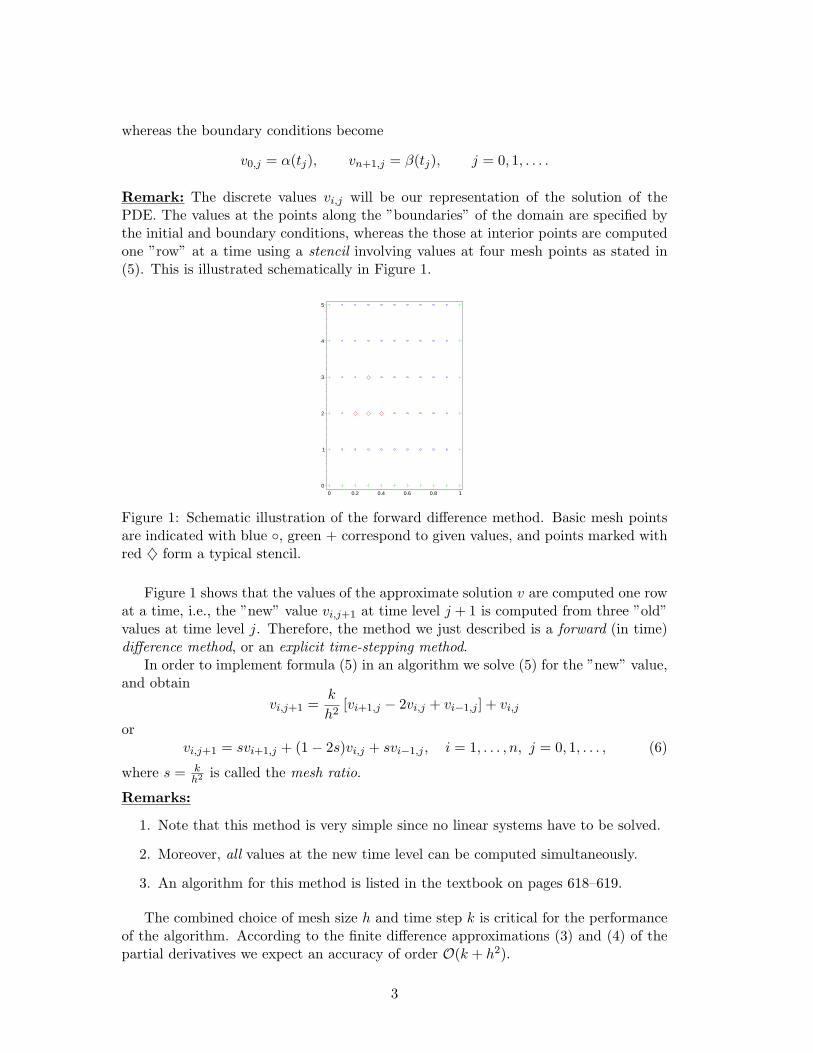
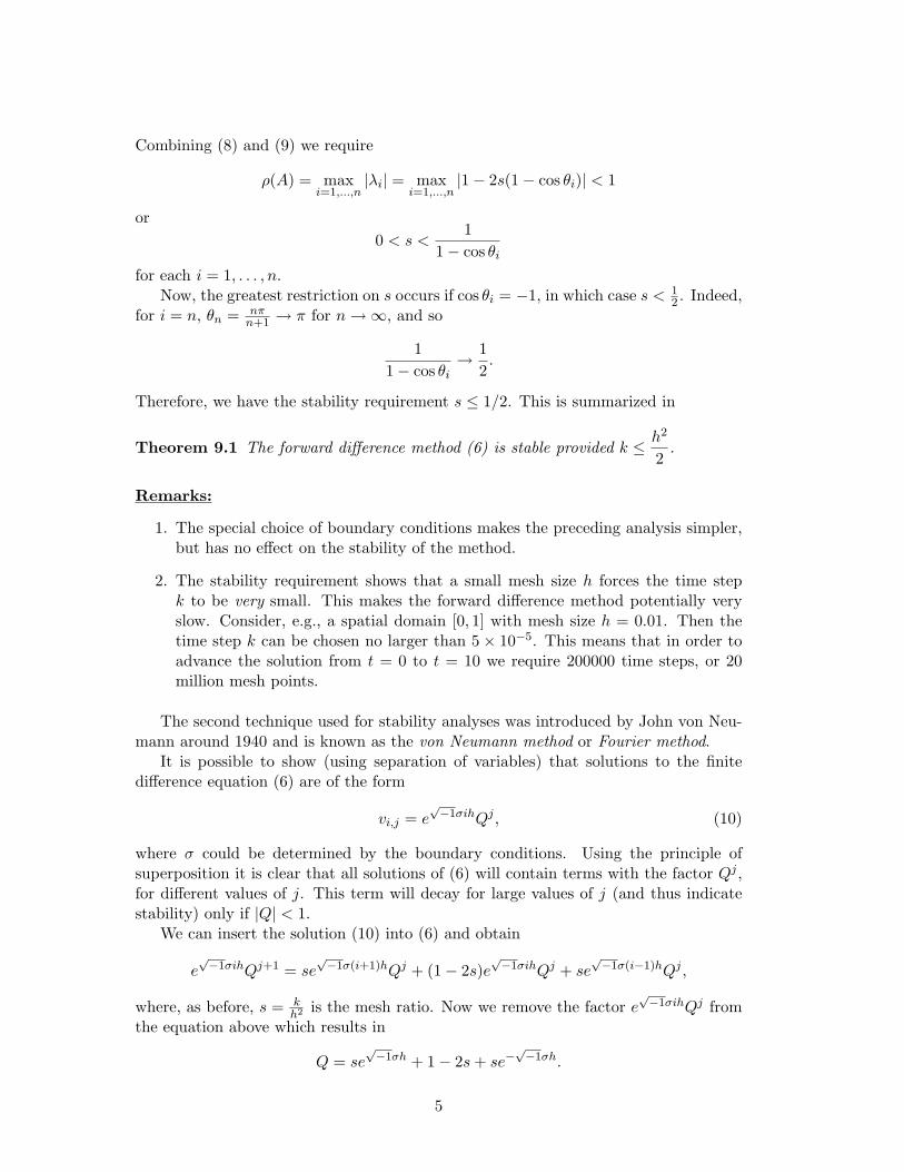
Remark: The discrete values vi,j will be our representation of the solution of thePDE. The values at the points along the ”boundaries” of the domain are specified bythe initial and boundary conditions, whereas the those at interior points are computedone ”row” at a time using a stencil involving values at four mesh points as stated in(5). This is illustrated schematically in Figure 1.
0
1
2
3
4
5
0 0.2 0.4 0.6 0.8 1
Figure 1: Schematic illustration of the forward difference method. Basic mesh pointsare indicated with blue , green + correspond to given values, and points marked withred ♦ form a typical stencil.
Figure 1 shows that the values of the approximate solution v are computed one rowat a time, i.e., the ”new” value vi,j+1 at time level j + 1 is computed from three ”old”values at time level j. Therefore, the method we just described is a forward (in time)difference method, or an explicit time-stepping method.
In order to implement formula (5) in an algorithm we solve (5) for the ”new” value,and obtain
vi,j+1 =k
h2[vi+1,j − 2vi,j + vi−1,j ] + vi,j
orvi,j+1 = svi+1,j + (1− 2s)vi,j + svi−1,j , i = 1, . . . , n, j = 0, 1, . . . , (6)
where s = kh2 is called the mesh ratio.
Remarks:
1. Note that this method is very simple since no linear systems have to be solved.
2. Moreover, all values at the new time level can be computed simultaneously.
3. An algorithm for this method is listed in the textbook on pages 618–619.
The combined choice of mesh size h and time step k is critical for the performanceof the algorithm. According to the finite difference approximations (3) and (4) of thepartial derivatives we expect an accuracy of order O(k + h2).
3
We now investigate the effects of h and k on the stability of the given method.
Stability Analysis
There are two standard techniques used for the stability analysis of PDEs. We nowillustrate them both.
First we use the matrix form. We simplify the following discussion by introducinghomogeneous boundary conditions, i.e., α(t) = β(t) ≡ 0. Otherwise we would havemore complicated first and last rows in the matrix below.
We begin by writing (6) in matrix form, i.e.,
Vj+1 = AVj , (7)
where Vj = [v1,j , v2,j , . . . , vn,j ]T is a vector that contains the values of the approximatesolution at all of the interior mesh points at any given time level j. The matrix A istridiagonal, and of the form
A =
1− 2s s 0 . . . 0
s 1− 2s s...
0. . . . . . . . . 0
... s 1− 2s s0 . . . 0 s 1− 2s
.
Note, however, that A appears on the right-hand side of (7) so that no system is solved,only a matrix-vector product is formed.
To investigate the stability of this method we assume that the initial data V0 arerepresented with some error E0, i.e.,
V0 = V0 + E0,
where V0 denotes the exact initial data. Then
V1 = AV0 = A(V0 + E0) = AV0 + AE0.
Advancing the solution further in time, i.e., iterating this formula, we get
Vj = AVj−1 = Aj V0 + AjE0.
Therefore, the initial error E0 is magnified by Aj at the j-th time level. In order tohave a stable and convergent method we need Ej = AjE0 → 0 as j →∞.
Taking norms we get
‖Ej‖ = ‖AjE0‖ ≤ ‖Aj‖‖E0‖,
so that we know that stability will be ensured if the spectral radius
ρ(A) < 1. (8)
One can show (see textbook pages 620–621) that the eigenvalues of A are given by
λi = 1− 2s(1− cos θi), θi =iπ
n + 1, i = 1, . . . , n. (9)
4
Combining (8) and (9) we require
ρ(A) = maxi=1,...,n
|λi| = maxi=1,...,n
|1− 2s(1− cos θi)| < 1
or0 < s <
11− cos θi
for each i = 1, . . . , n.Now, the greatest restriction on s occurs if cos θi = −1, in which case s < 1
2 . Indeed,for i = n, θn = nπ
n+1 → π for n →∞, and so
11− cos θi
→ 12.
Therefore, we have the stability requirement s ≤ 1/2. This is summarized in
Theorem 9.1 The forward difference method (6) is stable provided k ≤ h2
2.
Remarks:
1. The special choice of boundary conditions makes the preceding analysis simpler,but has no effect on the stability of the method.
2. The stability requirement shows that a small mesh size h forces the time stepk to be very small. This makes the forward difference method potentially veryslow. Consider, e.g., a spatial domain [0, 1] with mesh size h = 0.01. Then thetime step k can be chosen no larger than 5× 10⁻⁵. This means that in order toadvance the solution from t = 0 to t = 10 we require 200000 time steps, or 20million mesh points.
The second technique used for stability analyses was introduced by John von Neu-mann around 1940 and is known as the von Neumann method or Fourier method.
It is possible to show (using separation of variables) that solutions to the finitedifference equation (6) are of the form
vi,j = e√−1σihQj , (10)
where σ could be determined by the boundary conditions. Using the principle ofsuperposition it is clear that all solutions of (6) will contain terms with the factor Qj ,for different values of j. This term will decay for large values of j (and thus indicatestability) only if |Q| < 1.
We can insert the solution (10) into (6) and obtain
e√−1σihQj+1 = se
√−1σ(i+1)hQj + (1− 2s)e
√−1σihQj + se
√−1σ(i−1)hQj ,
where, as before, s = kh2 is the mesh ratio. Now we remove the factor e
√−1σihQj from
the equation above which results in
Q = se√−1σh + 1− 2s + se−
√−1σh.
5
With the help of Euler’s formula
e√−1φ = cos φ +
√−1 sinφ
and the trigonometric formula
sin2 φ =12
(1− cos 2φ)
the expression for Q can be simplified as follows:
Q = se√−1σh + 1− 2s + se−
√−1σh
= 1− 2s + 2s cos σh= 1− 2s (1− cos σh)
= 1− 4s sin2 σh
2.
From this it follows immediately that Q < 1 (since both h and k are positive, and thusalso s). To ensure also Q > −1 we need
4s sin2 σh
2≤ 2
ors sin2 σh
2≤ 1
2.
Since the sine term can approach 1, we need to impose the stability condition
s ≤ 12
which is the same condition obtained earlier via the matrix method.
Remarks:
1. Once stability is ensured, the forward difference method converges with orderO(k + h2) as stated earlier.
2. Computer Problem 9.1.1 illustrates the effect the choice of mesh size h and timestep k have on the stability of the forward difference method.
9.2 Implicit Methods for Parabolic PDEs
As we learned in the context of multistep methods for initial value problems, one canexpect a better stability behavior from an implicit method.
Therefore, we discretize the first-order time derivative as
ut(x, t) ≈ 1k
[u(x, t)− u(x, t− k)] , (11)
and so the formula corresponding to (5) now becomes
1h2
[vi+1,j − 2vi,j + vi−1,j ] =1k
[vi,j − vi,j−1] . (12)
6
0
1
2
3
4
5
0 0.2 0.4 0.6 0.8 1
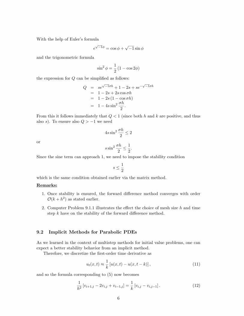
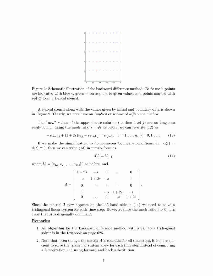
Figure 2: Schematic illustration of the backward difference method. Basic mesh pointsare indicated with blue , green + correspond to given values, and points marked withred ♦ form a typical stencil.
A typical stencil along with the values given by initial and boundary data is shownin Figure 2. Clearly, we now have an implicit or backward difference method.
The ”new” values of the approximate solution (at time level j) are no longer soeasily found. Using the mesh ratio s = k
h2 as before, we can re-write (12) as
−svi−1,j + (1 + 2s)vi,j − svi+1,j = vi,j−1, i = 1, . . . , n, j = 0, 1, . . . . (13)
If we make the simplification to homogeneous boundary conditions, i.e., α(t) =β(t) ≡ 0, then we can write (13) in matrix form as
AVj = Vj−1, (14)
where Vj = [v1,j , v2,j , . . . , vn,j ]T as before, and
A =
1 + 2s −s 0 . . . 0
−s 1 + 2s −s...
0. . . . . . . . . 0
... −s 1 + 2s −s0 . . . 0 −s 1 + 2s
.
Since the matrix A now appears on the left-hand side in (14) we need to solve atridiagonal linear system for each time step. However, since the mesh ratio s > 0, it isclear that A is diagonally dominant.
Remarks:
1. An algorithm for the backward difference method with a call to a tridiagonalsolver is in the textbook on page 625.
2. Note that, even though the matrix A is constant for all time steps, it is more effi-cient to solve the triangular system anew for each time step instead of computinga factorization and using forward and back substitution.
7
Stability Analysis
Under the same assumptions as for the forward difference method, the error nowpropagates according to
Vj = A−1Vj−1 =(A−1
)jV0 +
(A−1
)jE0,
with E0 the error present in the initial data. Therefore, this time we want
ρ(A−1
)< 1
for stability. The eigenvalues of A are given by
λi = 1 + 2s(1− cos θi), θi =iπ
n + 1, i = 1, . . . , n.
Since 0 < θi < π we know that | cos θi| < 1, and therefore λi > 1 for all i. Thus,ρ(A) > 1.
Finally, since the eigenvalues of A−1 are given by the reciprocals of the eigenvaluesof A we know that
ρ(A−1
)< 1,
and there is no stability restriction.
Theorem 9.2 The backward difference method (13) is unconditionally stable.
Remarks:
1. Again, having non-homogeneous boundary conditions does not affect the stabilityof the method.
2. The accuracy of the backward difference method is O(k +h2), which implies thatthe time step needs to be chosen small for high accuracy.
It has been suggested to use the symmetric difference approximation
ut(x, t) ≈ 12k
[u(x, t + k)− u(x, t− k)] , (15)
for the time derivative. This choice gives the following difference scheme an accuracyof order O(k2 + h2).
Using the above discretization of the time derivative, the difference version of theheat equation is
1h2
[vi+1,j − 2vi,j + vi−1,j ] =12k
[vi,j+1 − vi,j−1] .
orvi,j+1 =
2k
h2[vi+1,j − 2vi,j + vi−1,j ] + vi,j−1. (16)
This method is known as Richardson’s method. Richardson’s method can be viewed asan explicit method that requires two rows of initial values.
8
0
1
2
3
4
5
0 0.2 0.4 0.6 0.8 1
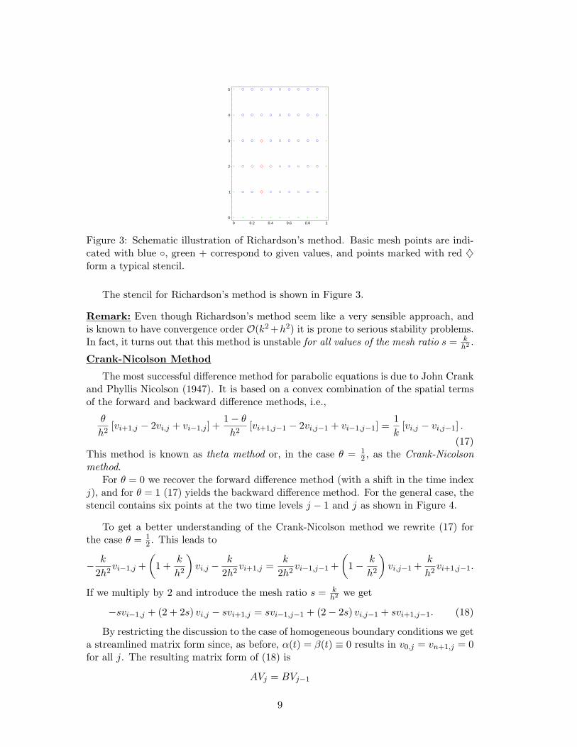
Figure 3: Schematic illustration of Richardson’s method. Basic mesh points are indi-cated with blue , green + correspond to given values, and points marked with red ♦form a typical stencil.
The stencil for Richardson’s method is shown in Figure 3.
Remark: Even though Richardson’s method seem like a very sensible approach, andis known to have convergence order O(k2 +h2) it is prone to serious stability problems.In fact, it turns out that this method is unstable for all values of the mesh ratio s = k
h2 .
Crank-Nicolson Method
The most successful difference method for parabolic equations is due to John Crankand Phyllis Nicolson (1947). It is based on a convex combination of the spatial termsof the forward and backward difference methods, i.e.,
θ
h2[vi+1,j − 2vi,j + vi−1,j ] +
1− θ
h2[vi+1,j−1 − 2vi,j−1 + vi−1,j−1] =
1k
[vi,j − vi,j−1] .
(17)This method is known as theta method or, in the case θ = 1
2 , as the Crank-Nicolsonmethod.
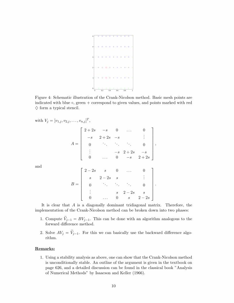
For θ = 0 we recover the forward difference method (with a shift in the time indexj), and for θ = 1 (17) yields the backward difference method. For the general case, thestencil contains six points at the two time levels j − 1 and j as shown in Figure 4.
To get a better understanding of the Crank-Nicolson method we rewrite (17) forthe case θ = 1
2 . This leads to
− k
2h2vi−1,j +
(1 +
k
h2
)vi,j −
k
2h2vi+1,j =
k
2h2vi−1,j−1 +
(1− k
h2
)vi,j−1 +
k
h2vi+1,j−1.
If we multiply by 2 and introduce the mesh ratio s = kh2 we get
−svi−1,j + (2 + 2s) vi,j − svi+1,j = svi−1,j−1 + (2− 2s) vi,j−1 + svi+1,j−1. (18)
By restricting the discussion to the case of homogeneous boundary conditions we geta streamlined matrix form since, as before, α(t) = β(t) ≡ 0 results in v0,j = vn+1,j = 0for all j. The resulting matrix form of (18) is
AVj = BVj−1
9
0
1
2
3
4
5
0 0.2 0.4 0.6 0.8 1
Figure 4: Schematic illustration of the Crank-Nicolson method. Basic mesh points areindicated with blue , green + correspond to given values, and points marked with red♦ form a typical stencil.
with Vj = [v1,j , v2,j , . . . , vn,j ]T ,
A =
2 + 2s −s 0 . . . 0
−s 2 + 2s −s...
0. . . . . . . . . 0
... −s 2 + 2s −s0 . . . 0 −s 2 + 2s
,
and
B =
2− 2s s 0 . . . 0
s 2− 2s s...
0. . . . . . . . . 0
... s 2− 2s s0 . . . 0 s 2− 2s
.
It is clear that A is a diagonally dominant tridiagonal matrix. Therefore, theimplementation of the Crank-Nicolson method can be broken down into two phases:
1. Compute Vj−1 = BVj−1. This can be done with an algorithm analogous to theforward difference method.
2. Solve AVj = Vj−1. For this we can basically use the backward difference algo-rithm.
Remarks:
1. Using a stability analysis as above, one can show that the Crank-Nicolson methodis unconditionally stable. An outline of the argument is given in the textbook onpage 626, and a detailed discussion can be found in the classical book ”Analysisof Numerical Methods” by Isaacson and Keller (1966).
10
2. Since the averaging of the forward and backward difference methods used for theCrank-Nicolson can be interpreted as an application of the (implicit) trapezoidrule for the time discretization, it follows that the order of accuracy of the Crank-Nicolson method is O(k2 + h2). Therefore, this method is much more efficient(for the same accuracy) than the forward or backward difference methods bythemselves.
3. If θ 6= 12 then the accuracy deteriorates to O(k + h2).
It is possible to ”fix” the Richardson method (16). To this end we replace the valuevi,j by the average of vi,j+1 and vi,j−1. We then end up with
vi,j+1 =2k
h2 + 2k[vi+1,j + vi−1,j ] +
h2 − 2k
h2 + 2kvi,j−1. (19)
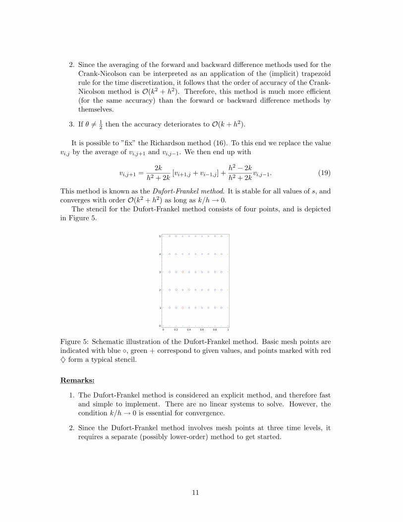
This method is known as the Dufort-Frankel method. It is stable for all values of s, andconverges with order O(k2 + h2) as long as k/h → 0.
The stencil for the Dufort-Frankel method consists of four points, and is depictedin Figure 5.
0
1
2
3
4
5
0 0.2 0.4 0.6 0.8 1
Figure 5: Schematic illustration of the Dufort-Frankel method. Basic mesh points areindicated with blue , green + correspond to given values, and points marked with red♦ form a typical stencil.
Remarks:
1. The Dufort-Frankel method is considered an explicit method, and therefore fastand simple to implement. There are no linear systems to solve. However, thecondition k/h → 0 is essential for convergence.
2. Since the Dufort-Frankel method involves mesh points at three time levels, itrequires a separate (possibly lower-order) method to get started.
11
9.3 Finite Differences for Elliptic PDEs
We use Laplace’s equation in the unit square as our model problem, i.e.,
uxx + uyy = 0, (x, y) ∈ Ω = (0, 1)2,u(x, y) = g(x, y), (x, y) on ∂Ω. (20)
This problem arises, e.g., when we want to determine the steady-state temperaturedistribution u in a square region with prescribed boundary temperature g. Of course,this simple problem can be solved analytically using Fourier series.
However, we are interested in numerical methods. Therefore, in this section, we usethe usual finite difference discretization of the partial derivatives, i.e.,
uxx(x, y) =1h2
[u(x + h, y)− 2u(x, y) + u(x− h, y)] +O(h2) (21)
anduyy(x, y) =
1h2
[u(x, y + h)− 2u(x, y) + u(x, y − h)] +O(h2). (22)
The computational grid introduced in the domain Ω = [0, 1]2 is now
(xi, yj) = (ih, jh), i, j = 0, . . . , n + 1,
with mesh size h = 1n+1 .
Using again the compact notation
vi,j = u(xi, yj), vi+1,j = u(xi + h, yj), etc.,
Laplace’s equation (20) turns into the difference equation
1h2
[vi−1,j − 2vi,j + vi+1,j ] +1h2
[vi,j−1 − 2vi,j + vi,j+1] = 0. (23)
This equation can be rewritten as
4vi,j − vi−1,j − vi+1,j − vi,j−1 − vi,j+1 = 0. (24)
This is the method referred to several times last semester.
Example: Let’s consider a computational mesh of 5× 5 points, i.e., h = 14 , or n = 3.
Discretizing the boundary conditions in (20), the values of the approximate solutionaround the boundary
v0,j , v4,j j = 0, . . . , 4,vi,0, vi,4 i = 0, . . . , 4,
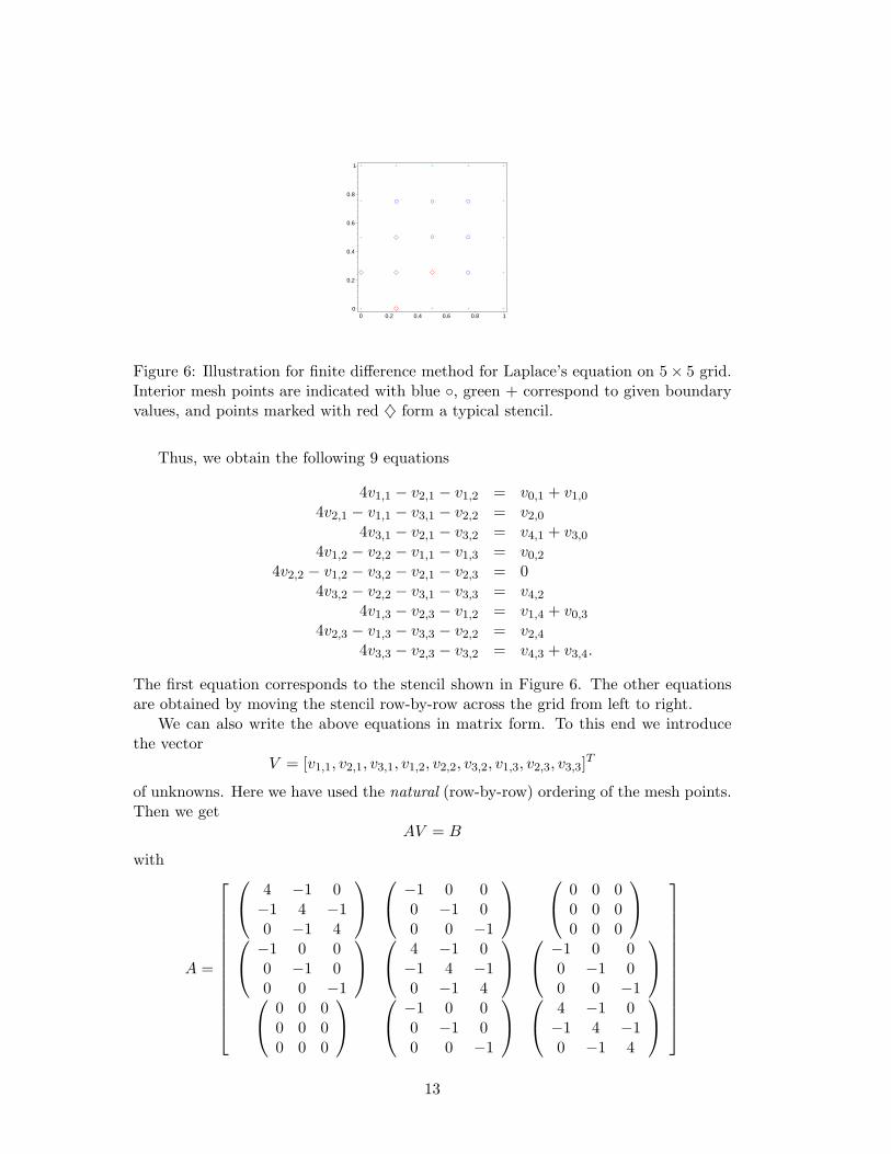
are determined by the appropriate values of g. There remain 9 points in the interiorthat have to be determined using the stencil (24). Figure 6 illustrates one instance ofthis task. By applying the stencil to each of the interior points, we obtain 9 conditionsfor the 9 undetermined values.
12
0
0.2
0.4
0.6
0.8
1
0 0.2 0.4 0.6 0.8 1
Figure 6: Illustration for finite difference method for Laplace’s equation on 5× 5 grid.Interior mesh points are indicated with blue , green + correspond to given boundaryvalues, and points marked with red ♦ form a typical stencil.
Thus, we obtain the following 9 equations
4v1,1 − v2,1 − v1,2 = v0,1 + v1,0
4v2,1 − v1,1 − v3,1 − v2,2 = v2,0
4v3,1 − v2,1 − v3,2 = v4,1 + v3,0
4v1,2 − v2,2 − v1,1 − v1,3 = v0,2
4v2,2 − v1,2 − v3,2 − v2,1 − v2,3 = 04v3,2 − v2,2 − v3,1 − v3,3 = v4,2
4v1,3 − v2,3 − v1,2 = v1,4 + v0,3
4v2,3 − v1,3 − v3,3 − v2,2 = v2,4
4v3,3 − v2,3 − v3,2 = v4,3 + v3,4.
The first equation corresponds to the stencil shown in Figure 6. The other equationsare obtained by moving the stencil row-by-row across the grid from left to right.
We can also write the above equations in matrix form. To this end we introducethe vector
V = [v1,1, v2,1, v3,1, v1,2, v2,2, v3,2, v1,3, v2,3, v3,3]T
of unknowns. Here we have used the natural (row-by-row) ordering of the mesh points.Then we get
AV = B
with
A =
4 −1 0−1 4 −10 −1 4
−1 0 00 −1 00 0 −1
0 0 00 0 00 0 0
−1 0 0
0 −1 00 0 −1
4 −1 0−1 4 −10 −1 4
−1 0 00 −1 00 0 −1
0 0 0
0 0 00 0 0
−1 0 00 −1 00 0 −1
4 −1 0−1 4 −10 −1 4
13
and
B =
v0,1 + v1,0
v2,0
v4,1 + v3,0
v0,2
0v4,2
v1,4 + v0,3
v2,4
v4,3 + v3,4
.
We can see that A is a block-tridiagonal matrix of the form
A =
T −I O−I T −IO −I T
.
In general, for problems with n × n interior mesh points, A will be of size n2 × n2
(since there are n2 unknown values at interior mesh points), but contain no more than5n2 nonzero entries (since equation (24) involves at most 5 points at one time). Thus,A is a classical example of a sparse matrix. Moreover, A still has a block-tridiagonalstructure
A =
T −I O . . . O
−I T −I...
O. . . . . . . . . O
... −I T −IO . . . O −I T
with n× n blocks
T =
4 −1 0 . . . 0
−1 4 −1...
0. . . . . . . . . 0
... −1 4 −10 . . . 0 −1 4
as well as n× n identity matrices I, and zero matrices O.
Remarks:
1. Since A is sparse (and symmetric positive definite) it lends itself to an applica-tion of Gauss-Seidel iteration (see Chapter 4.6 of the previous semester). Afterinitializing the values at all mesh points (including those along the boundary) tosome appropriate value (in many cases zero will work), we can simply iterate withformula (24), i.e., we obtain the algorithm fragment for M steps of Gauss-Seideliteration
14
for k = 1 to M do
for i = 1 to n dofor j = 1 to n do
vi,j = (vi−1,j + vi+1,j + vi,j−1 + vi,j+1) /4end
end
end
Note that the matrix A never has to be fully formed or stored during the com-putation.
2. State-of-the-art algorithms for the Laplace (or nonhomogeneous Poisson) equa-tion are so-called fast Poisson solvers based on the fast Fourier transform, ormultigrid methods.
9.4 Galerkin and Ritz Methods for Elliptic PDEs
Galerkin MethodWe begin by introducing a generalization of the collocation method we saw earlier
for two-point boundary value problems. Consider the PDE
Lu(x) = f(x), (25)
where L is a linear elliptic partial differential operator such as the Laplacian
L =∂2
∂x2+
∂2
∂y2+
∂2
∂z2, x = (x, y, z) ∈ IR3 .
At this point we will not worry about the boundary conditions that should be posedwith (25).
As with the collocation method we will obtain the approximate solution in theform of a function (instead of as a collection of discrete values). Therefore, we needan approximation space U = spanu1, . . . , un, so that we are able to represent theapproximate solution as
u =n∑
j=1
cjuj , uj ∈ U . (26)
Using the linearity of L we have
Lu =n∑
j=1
cjLuj .
We now need to come up with n (linearly independent) conditions to determine the nunknown coefficients cj in (26). If Φ1, . . . ,Φn is a linearly independent set of linearfunctionals, then
Φi
n∑j=1
cjLuj − f
= 0, i = 1, . . . , n, (27)
15
is an appropriate set of conditions. In fact, this leads to a system of linear equations
Ac = b
with matrix
A =
Φ1Lu1 Φ1Lu2 . . . Φ1Lun
Φ2Lu1 Φ2Lu2 . . . Φ2Lun...
......
ΦnLu1 ΦnLu2 . . . ΦnLun
,
coefficient vector c = [c1, . . . , cn]T , and right-hand side vector
b =
Φ1fΦ2f
...Φnf
.
Two popular choices are
1. Point evaluation functionals, i.e., Φi(v) = v(xi), where x1, . . . ,xn is a set ofpoints chosen such that the resulting conditions are linearly independent, and vis some function with appropriate smoothness. With this choice (27) becomes
n∑j=1
cjLuj(xi) = f(xi), i = 1, . . . , n,
and we now have a extension of the collocation method discussed in Section 8.11to elliptic PDEs is the multi-dimensional setting.
2. If we let Φi(v) = 〈ui, v〉, an inner product of the basis function ui with an appro-priate test function v, then (27) becomes
n∑j=1
cj〈ui, Luj〉 = 〈ui, f〉, i = 1, . . . , n.
This is the classical Galerkin method.
Ritz-Galerkin Method
For the following discussion we pick as a model problem a multi-dimensional Poissonequation with homogeneous boundary conditions, i.e.,
−∇2u = f in Ω, (28)u = 0 on ∂Ω,
with domain Ω ⊂ IRd. This problem describes, e.g., the steady-state solution of avibrating membrane (in the case d = 2 with shape Ω) fixed at the boundary, andsubjected to a vertical force f .
16
The first step for the Ritz-Galerkin method is to obtain the weak form of (28). Thisis accomplished by choosing a function v from a space U of smooth functions, and thenforming the inner product of both sides of (28) with v, i.e.,
−〈∇2u, v〉 = 〈f, v〉. (29)
To be more specific, we let d = 2 and take the inner product
〈u, v〉 =∫∫Ω
u(x, y)v(x, y)dxdy.
Then (29) becomes
−∫∫Ω
(uxx(x, y) + uyy(x, y))v(x, y)dxdy =∫∫Ω
f(x, y)v(x, y)dxdy. (30)
In order to be able to complete the derivation of the weak form we now assume thatthe space U of test functions is of the form
U = v : v ∈ C2(Ω), v = 0 on ∂Ω,
i.e., besides having the necessary smoothness to be a solution of (28), the functionsalso satisfy the boundary conditions.
Now we rewrite the left-hand side of (30):∫∫Ω
(uxx + uyy) vdxdy =∫∫Ω
[(uxv)x + (uyv)y − uxvx − uyvy] dxdy
=∫∫Ω
[(uxv)x + (uyv)y] dxdy −∫∫Ω
[uxvx − uyvy] dxdy.(31)
By using Green’s Theorem (integration by parts)∫∫Ω
(Px + Qy)dxdy =∫
∂Ω(Pdy −Qdx)
the first integral on the right-hand side of (31) turns into∫∫Ω
[(uxv)x + (uyv)y] dxdy =∫
∂Ω(uxvdy − uyvdx) .
Now the special choice of U , i.e., the fact that v satisfies the boundary conditions,ensures that this term vanishes. Therefore, the weak form of (28) is given by∫∫
Ω
[uxvx + uyvy] dxdy =∫∫Ω
fvdxdy.
Another way of writing the previous formula is of course∫∫Ω
∇u · ∇vdxdy =∫∫Ω
fvdxdy. (32)
17
To obtain a numerical method we now need to require U to be finite-dimensionalwith basis u1, . . . , un. Then we can represent the approximate solution uh of (28) as
uh =n∑
j=1
cjuj . (33)
The superscript h indicates that the approximate solution is obtained on some under-lying discretization of Ω with mesh size h.
Remarks:
1. In practice there are many ways of discretizing Ω and selecting U .
(a) For example, regular (tensor product) grids can be used. Then U can consistof tensor products of piecewise polynomials or B-spline functions that satisfythe boundary conditions of the PDE.
(b) It is also possible to use irregular (triangulated) meshes, and again definepiecewise (total degree) polynomials or splines on triangulations satisfyingthe boundary conditions.
(c) More recently, meshfree approximation methods have been introduced aspossible choices for U .
2. In the literature the piecewise polynomial approach is usually referred to as thefinite element method.
3. The discretization of Ω will almost always result in a computational domain thathas piecewise linear (Lipschitz-continuous) boundary.
We now return to the discussion of the general numerical method. Once we havechosen a basis for the approximation space U , then it becomes our goal to determinethe coefficients cj in (33). By inserting uh into the weak form (32), and selecting astrial functions v the basis functions of U we obtain a system of equations∫∫
Ω
∇uh · ∇uidxdy =∫∫Ω
fuidxdy, i = 1, . . . , n.
Using the representation (33) of uh we get∫∫Ω
∇
n∑j=1
cjuj
· ∇uidxdy =∫∫Ω
fuidxdy, i = 1, . . . , n,
or by linearityn∑
j=1
cj
∫∫Ω
∇uj · ∇uidxdy =∫∫Ω
fuidxdy, i = 1, . . . , n. (34)
This last set of equations is known as the Ritz-Galerkin method and can be written inmatrix form
Ac = b,
18
where the stiffness matrix A has entries
Ai,j =∫∫Ω
∇uj · ∇uidxdy.
Remarks:
1. The stiffness matrix is usually assembled element by element, i.e., the contributionto the integral over Ω is split into contributions for each element (e.g., rectangleor triangle) of the underlying mesh.
2. Depending on the choice of the (finite-dimensional) approximation space U andunderlying discretization, the matrix will have a well-defined structure. This isone of the most important applications driving the design of efficient linear systemsolvers.
How does solving the Ritz-Galerkin equations (34) relate to the solution of thestrong form (28) of the PDE? First, we remark that the left-hand side of (32) can beinterpreted as a new inner product
[u, v] =∫∫Ω
∇u · ∇vdxdy (35)
on the space of functions whose first derivatives are square integrable and that vanishon ∂Ω. This space is a Sobolev space, usually denoted by H1
0 (Ω).The inner product [·, ·] induces a norm ‖v‖ = [v, v]1/2 on H1
0 (Ω). Now, usingthis norm, the best approximation to u from H1
0 (Ω) is given by the function uh thatminimizes ‖u − uh‖. Since we define our numerical method via the finite-dimensionalsubspace U of H1
0 (Ω), we need to find uh such that
u− uh ⊥ U
or, using the basis of U , [u− uh, ui
]= 0, i = 1, . . . , n.
Replacing uh with its expansion in terms of the basis of U we haveu−n∑
j=1
cjuj , ui
= 0, i = 1, . . . , n,
orn∑
j=1
cj [uj , ui] = [u, ui], i = 1, . . . , n. (36)
The right-hand side of this formula contains the exact solution u, and therefore is notuseful for a numerical scheme. However, by (35) and the weak form (32) we have
[u, ui] =∫∫Ω
∇u · ∇uidxdy
19
=∫∫Ω
fuidxdy.
Since the last expression corresponds to the inner product 〈f, ui〉, (36) can be viewedas
n∑j=1
cj [uj , ui] = 〈f, ui〉, i = 1, . . . , n,
which is nothing but the Ritz-Galerkin method (34).
The best approximation property in the Sobolev space H10 (Ω) can also be inter-
preted as an energy minimization principle. In fact, a smooth solution of the Poissonproblem (28) minimizes the energy functional
E(u) =12
∫∫Ω
∇2udxdy −∫∫Ω
fudxdy
over all smooth functions that vanish on the boundary of Ω. By considering the energyof nearby solutions u + λv, with arbitrary real λ we see that
E(u + λv) =12
∫∫Ω
∇(u + λv) · ∇(u + λv)dxdy −∫∫Ω
f(u + λv)dxdy
=12
∫∫Ω
∇u · ∇udxdy + λ
∫∫Ω
∇u · ∇vdxdy +λ2
2
∫∫Ω
∇v · ∇vdxdy
−∫∫Ω
fudxdy − λ
∫∫Ω
fvdxdy
= E(u) + λ
∫∫Ω
[∇u · ∇v − fv] dxdy +λ2
2
∫∫Ω
∇2vdxdy
The right-hand side is a quadratic polynomial in λ, so that for a minimum, the term∫∫Ω
[∇u · ∇v − fv] dxdy
must vanish for all v. This is again the weak formulation (32).A discrete ”energy norm” is then given by the quadratic form
E(uh) =12cT Ac− bc
where A is the stiffness matrix, and c is such that the Ritz-Galerkin system (34)
Ac = b
is satisfied.
20
Example: One of the most popular finite element versions is based on the use ofpiecewise linear C0 polynomials (built either on a regular grid, or on a triangularpartition of Ω). The basis functions ui are ”hat functions”, i.e., functions that arepiecewise linear, have value one at one of the vertices, and zero at all of its neighbors.This choice makes it very easy to satisfy the homogeneous Dirichlet boundary conditionsof the model problem exactly (along a polygonal boundary).
Since the gradients of piecewise linear functions are constant, the entries of thestiffness matrix essentially boil down to the areas of the underlying mesh elements.
Therefore, in this case, the Ritz-Galerkin method is very easily implemented. Wegenerate some examples with Matlab’s PDE toolbox pdetool.
It is not difficult to verify that the stiffness matrix for our example is symmetricand positive definite. Since the matrix is also very sparse due to the fact that the ”hat”basis functions have a very localized support, efficient iterative solvers can be applied.Moreover, it is known that the piecewise linear FEM converges with order O(h2).
Remarks:
1. The Ritz-Galerkin method was independently introduced by Walther Ritz (1908)and Boris Galerkin (1915).
2. In the textbook this method is referred to as the Rayleigh-Ritz method. Manyvariations in terminology seem to exist indicating only slight (or no) differencesin methodology.
3. The finite element method is one of the most-thoroughly studied numerical meth-ods. Many textbooks on the subject exist, e.g., ”The Mathematical Theory ofFinite Element Methods” by Brenner and Scott (1994), ”An Analysis of the FiniteElement Method” by Strang and Fix (1973), or ”The Finite Element Method”by Zienkiewicz and Taylor (2000).
4. Even though the use of piecewise linear finite elements is very simple, there aremany problems that arise with higher-order methods, mesh refinement, or withthe generation of finite element meshes in higher space dimensions. This is wheremeshfree approximation methods are trying to establish themselves as a viablealternative.
9.5 Characteristics
We start with the simple advection equation
ut(x, t) = −cux(x, t), −∞ < x < ∞, t ≥ 0, (37)
where c is some nonzero constant. This problem has a unique solution as soon as wespecify an initial condition
u(x, 0) = f(x), −∞ < x < ∞.
21
A pure initial value problem of this type is called a Cauchy problem. It is easily verified(using the chain rule) that the solution to this problem is given by
u(x, t) = f(x− ct).
This shows us that the solution u is simply a shifted version of the initial profile f . Infact, the initial profile ”moves to the right with velocity c”. Therefore, the PDE (37)is also referred to as the transport equation or one-way wave equation.
A characteristic curve or simply characteristic is a curve in the (x, t)-plane on whichthe solution u of a PDE is constant. For the advection equation we have
d
dtu(x(t), t) = ux
dx(t)dt
+ ut. (38)
Since ut = −cux we see that the solution u is constant, i.e.,
d
dtu(x(t), t) = 0
ifdx(t)
dt= c. (39)
This is an ODE that determines the characteristic x = x(t) of the advection equation.From (39) it is clear that the characteristics of the advection equation are the lines
x(t) = ct + x0.
Remark: The left-hand side of equation (38) can be interpreted as the change as expe-rienced by a moving observer, whereas the two parts on the right-hand side representthe change due to the fact that the the observer is moving into a region of possiblydifferent u, and the change of the solution at a fixed point. Our discussion of charac-teristics shows that an observer moving along with speed c will see no change in thesolution.
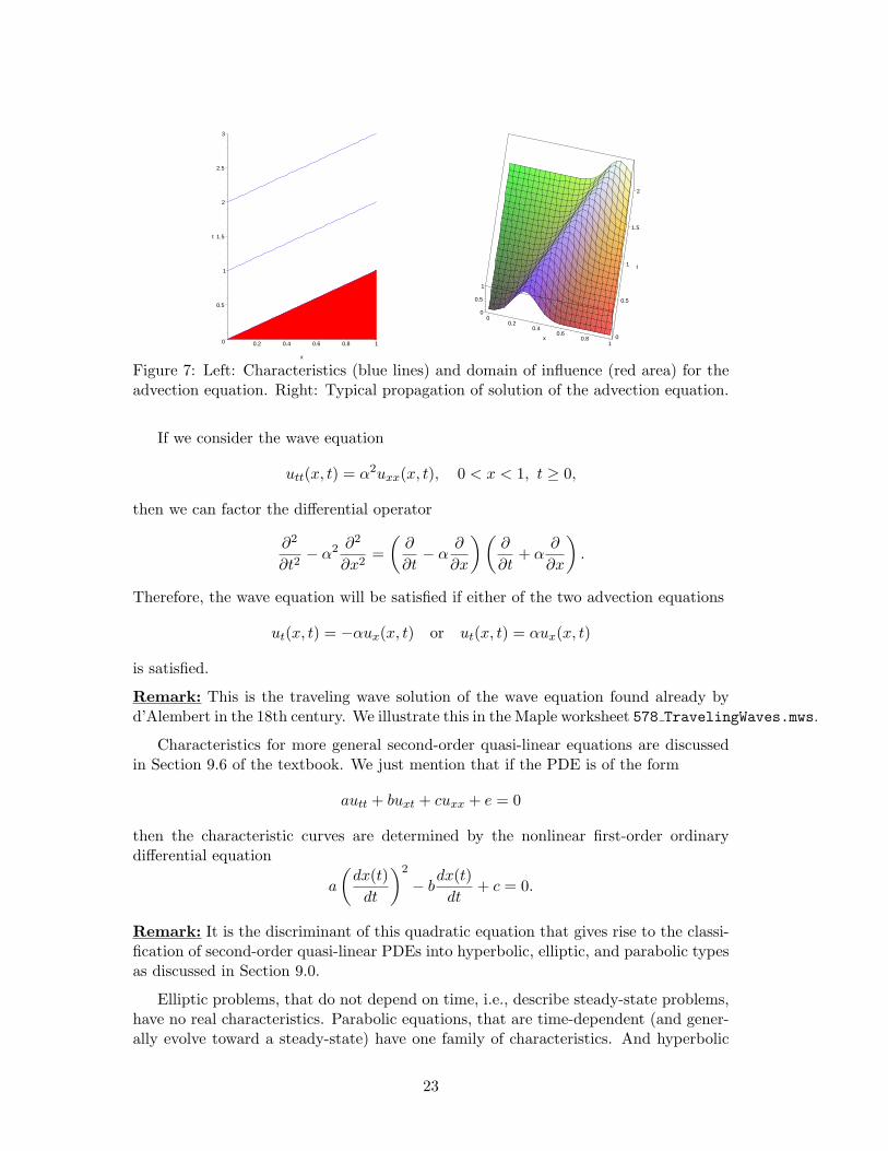
Characteristics give us fundamental insight into the solution of a partial differentialequation. Assume, e.g., that we have specified initial values for the advection equation(37) only on the finite interval 0 ≤ x ≤ 1. If we consider the domain (x, t) : 0 ≤ x ≤1, t ≥ 0, then the given initial values will determine the solution only in part of thisdomain. The left part of Figure 7 illustrates this fact for a positive value of c.
The right part of Figure 7 shows how the solution ”propagates along characteris-tics”. This is also clear when we recall that a characteristic curve is the location ofpoints in the (x, t)-plane along which the solution of the PDE is constant.
In order to obtain the solution on the remainder (unshaded part) of the domain weneed to specify boundary values along the line x = 0. However, specifying values alongthe other boundary, x = 1, would possibly overdetermine the problem.
If we want to study characteristics for general second-order quasi-linear PDEs thenthe situation is more complicated.
22
0
0.5
1
1.5
2
2.5
3
t
0.2 0.4 0.6 0.8 1
x
00.2
0.40.6
0.81
x 0
0.5
1
1.5
2
t
0
0.5
1
Figure 7: Left: Characteristics (blue lines) and domain of influence (red area) for theadvection equation. Right: Typical propagation of solution of the advection equation.
If we consider the wave equation
utt(x, t) = α2uxx(x, t), 0 < x < 1, t ≥ 0,
then we can factor the differential operator
∂2
∂t2− α2 ∂2
∂x2=
(∂
∂t− α
∂
∂x
) (∂
∂t+ α
∂
∂x
).
Therefore, the wave equation will be satisfied if either of the two advection equations
ut(x, t) = −αux(x, t) or ut(x, t) = αux(x, t)
is satisfied.
Remark: This is the traveling wave solution of the wave equation found already byd’Alembert in the 18th century. We illustrate this in the Maple worksheet 578 TravelingWaves.mws.
Characteristics for more general second-order quasi-linear equations are discussedin Section 9.6 of the textbook. We just mention that if the PDE is of the form
autt + buxt + cuxx + e = 0
then the characteristic curves are determined by the nonlinear first-order ordinarydifferential equation
a
(dx(t)
dt
)2
− bdx(t)
dt+ c = 0.
Remark: It is the discriminant of this quadratic equation that gives rise to the classi-fication of second-order quasi-linear PDEs into hyperbolic, elliptic, and parabolic typesas discussed in Section 9.0.
Elliptic problems, that do not depend on time, i.e., describe steady-state problems,have no real characteristics. Parabolic equations, that are time-dependent (and gener-ally evolve toward a steady-state) have one family of characteristics. And hyperbolic
23
PDEs, that are time-dependent (but do not evolve toward a steady-state) have twoindependent families of characteristics. If these characteristics cross, then the solutioncan develop discontinuities or shocks (even for smooth initial data). This is one of themajor difficulties associated with the solution of hyperbolic PDEs.
Since hyperbolic PDEs are conservative, i.e., the ”energy” of the system remainsconstant over time (such as in the perpetual vibrations for the wave equation), it isimportant to ensure that numerical schemes are also conservative. We will follow upon this idea in Section 9.7.Remark: A numerical method, called the method of characteristics, asks the userto determine the ordinary differential equation that defines the characteristics of agiven partial differential equations. Then a numerical ODE solver is used to solve thisODE, resulting in level curves for the solution. Once these level curves are found, itis possible to use another ODE solver to integrate the PDE (which is now an ODE)along the characteristic (see (39)).
9.6 Finite Differences for Hyperbolic PDEs
Before we study specialized numerical methods for conservation laws, we take a look ata straightforward finite difference scheme. This material is touched on in Section 9.7 ofthe textbook. We now consider as a model problem the one-dimensional wave equation
utt(x, t) = α2uxx(x, t), 0 < x < 1, t ≥ 0,u(x, 0) = f(x), 0 ≤ x ≤ 1,ut(x, 0) = g(x), 0 ≤ x ≤ 1,u(0, t) = u(1, t) = 0, t ≥ 0.
This model is used to describe the vibrations of a string of unit length fixed at bothends subject to an initial displacement f(x) and initial velocity g(x).
In order to be able to formulate finite differences we need a discrete approximationof the second derivatives. We use the symmetric formulas
utt =1k2
[u(x, t + k)− 2u(x, t) + u(x, t− k)] +O(k2)
anduxx =
1h2
[u(x + h, t)− 2u(x, t) + u(x− h, t)] +O(h2).
Here we have discretized the computational domain with
xi = ih, i = 0, . . . , n + 1,tj = jk, j ≥ 0.
As always, h = 1n+1 is the mesh size and k is the time step. Also, we use the notation
vi,j = u(xi, tj), etc..Inserting the finite difference approximations into the wave equation we get
1k2
[vi,j+1 − 2vi,j + vi,j−1] =α2
h2[vi+1,j − 2vi,j + vi−1,j ] . (40)
24
Finally, we can introduce the mesh ratio s =(
αkh
)2, and solve (40) for the value at
time level j + 1, i.e.,
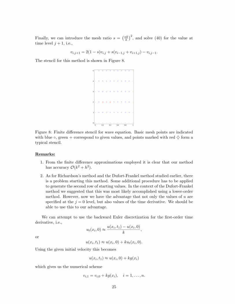
vi,j+1 = 2(1− s)vi,j + s(vi−1,j + vi+1,j)− vi,j−1.
The stencil for this method is shown in Figure 8.
0
1
2
3
4
5
0 0.2 0.4 0.6 0.8 1
Figure 8: Finite difference stencil for wave equation. Basic mesh points are indicatedwith blue , green + correspond to given values, and points marked with red ♦ form atypical stencil.
Remarks:
1. From the finite difference approximations employed it is clear that our methodhas accuracy O(k2 + h2).
2. As for Richardson’s method and the Dufort-Frankel method studied earlier, thereis a problem starting this method. Some additional procedure has to be appliedto generate the second row of starting values. In the context of the Dufort-Frankelmethod we suggested that this was most likely accomplished using a lower-ordermethod. However, now we have the advantage that not only the values of u arespecified at the j = 0 level, but also values of the time derivative. We should beable to use this to our advantage.
We can attempt to use the backward Euler discretization for the first-order timederivative, i.e.,
ut(xi, 0) ≈ u(xi, t1)− u(xi, 0)k
,
oru(xi, t1) ≈ u(xi, 0) + kut(xi, 0).
Using the given initial velocity this becomes
u(xi, t1) ≈ u(xi, 0) + kg(xi)
which gives us the numerical scheme
vi,1 = vi,0 + kg(xi), i = 1, . . . , n.
25
This lets us advance the information given at the j = 0 level to the first row of thecomputational mesh at j = 1. However, the backward Euler discretization is orderO(k) only, so that the entire numerical method will be O(k + h2) only.
In order to get a second-order accurate formula for this first step we employ a Taylorexpansion of u with respect to the time variable, i.e.,
u(xi, t1) ≈ u(xi, 0) + kut(xi, 0) +k2
2utt(xi, 0). (41)
Now, the wave equation tells us that
utt(xi, 0) = α2uxx(xi, 0).
Moreover, since u = f for time t = 0 we get (provided f is smooth enough)
utt(xi, 0) = α2f ′′(xi),
and so the Taylor expansion (41) becomes
u(xi, t1) ≈ u(xi, 0) + kut(xi, 0) +k2α2
2f ′′(xi).
This allows us to express the values at the j = 1 level as
vi,1 = vi,0 + kg(xi) +k2α2
2f ′′(xi).
Using again a symmetric finite difference approximation for f ′′ we have
vi,1 = vi,0 + kg(xi) +k2α2
21h2
[f(xi+1)− 2f(xi) + f(xi−1)] .
Since f(xi) = u(xi, 0) = vi,0 we arrive at
vi,1 = (1− s)vi,0 +s
2[vi−1,0 + vi+1,0] + kg(xi), (42)
where we have used the mesh ratio s =(
αkh
)2.
Remarks:
1. Formula (42) is second-order accurate in time. Therefore, the finite differencemethod consisting of (42) for the first step, and (40) for subsequent steps is oforder O(k2 + h2).
2. Once the first two rows of values have be obtained, the method proceeds in anexplicit way, i.e., no linear systems have to be solved.
3. However, as with all explicit methods there are restrictions on the mesh ratio inorder to maintain stability. For this method we have s ≤ 1.
26
9.7 Flux Conservation for Hyperbolic PDEs
We mentioned earlier that hyperbolic partial differential equations are conservative.This was clearly illustrated by the simple advection equation (37). It is customary tore-write hyperbolic PDEs in the so-called flux conservative form. We illustrate thiswith the wave equation
utt(x, t) = α2uxx(x, t), 0 < x < 1, t ≥ 0.
If we introduce the new variables
v = αux, and w = ut
then
vt = αuxt
wx = utx
so that vt = αwx. Since we also have
vx = αuxx
wt = utt
we see that the wave equation is equivalent to a system of two coupled first-order partialdifferential equations
vt = αwx
wt = αvx.
Remark: In physics these equations arise in the study of one-dimensional electromag-netic waves, and are known as Maxwell’s equations.
To get the standard flux conservative form of a hyperbolic conservation law weintroduce matrix-vector notation
u =[
vw
], F (u) =
[0 −α−α 0
]u,
so thatut = −F (u)x.
The function F (u) is called the flux of the problem.
Remarks:
1. If the system consists of only one equation, then we recover the advection equation(37).
2. An excellent book on hyperbolic conservation laws (covering theory and numerics)is ”Numerical Methods for Conservation Laws” by Randy LeVeque (1992).
27
We now investigate numerical methods for the simple conservation law
ut(x, t) = −cux(x, t), 0 < x < 1, t ≥ 0,u(x, 0) = f(x), 0 ≤ x ≤ 1.
The most natural finite difference approach is based on the derivative approximations
ut(x, t) =1k
[u(x, t + k)− u(x, t)] +O(k)
ux(x, t) =12h
[u(x + h, t)− u(x− h, t)] +O(h2).
Using the standard discretization
xi = ih, i = 0, . . . , n + 1,tj = jk, j ≥ 0,
with mesh size h = 1n+1 and time step k, as well as the notation vi,j = u(xi, tj), we
obtain1k
[vi,j+1 − vi,j ] = − c
2h[vi+1,j − vi−1,j ]
orvi,j+1 = −kc
2h[vi+1,j − vi−1,j ] + vi,j . (43)
Remarks:
1. The method (43) is an explicit, and therefore fast method.
2. However, as we will show next, this method is completely useless since it is un-conditionally unstable.
3. We use the advection equation with a smooth step function as initial conditionto illustrate the performance of this method. The (slightly modified) Matlabprogram transport.m (with menu option ”forward Euler in time / centered dif-ferences in space”) originally written by Stefan Hueber, University of Stuttgart,Germany, serves this purpose.
We now perform the von Neumann stability analysis to verify this claim. Let’sassume that the solution of the model problem is of the form
vi,j = e√−1iβhejλk
= e√−1iβh
(eλk
)j(44)
obtained via separation of variables (the so-called plane wave solution). The questionis what the long time behavior of this solution is, i.e., we are interested in
limj→∞
vi,j .
Since (44) contains an oscillatory as well as an exponentially growing component, wewill need |eλk| ≤ 1 for stability.
28
In order to compute the amplification factor eλk we substitute (44) into our numer-ical method (43). This yields
e√−1iβhe(j+1)λk = −kc
2h
[e√−1(i+1)βh − e
√−1(i−1)βh
]ejλk + e
√−1iβhejλk.
Division by e√−1iβhejλk gives us
eλk = −kc
2h
[e√−1βh − e−
√−1βh
]+ 1
= 1−√−1
kc
hsinβh. (45)
Here we have used the complex trigonometric identity
sin z =e√−1z − e−
√−1z
2√−1
.
From (45) it is clear that|eλk| ≥ 1
for all positive time steps k since eλk lies somewhere on the line <(z) = 1 in the complexplane. Therefore the method is – as claimed – unconditionally unstable.
Lax-Friedrichs Method
Earlier, we were able to ”fix” Richardson’s method for parabolic PDEs by replacingvi,j by an average of neighboring points (in time). This led to the Dufort-Frankelmethod.
Now we replace vi,j in (43) by an average of neighboring values in space, i.e., weinsert
vi,j =vi+1,j + vi−1,j
2into (43). That results in
vi,j+1 =vi+1,j + vi−1,j
2− kc
2h[vi+1,j − vi−1,j ] . (46)
This is known as the Lax-Friedrichs method due to Peter Lax and Kurt Friedrichs.Introducing, as always, the mesh ratio s = kc
2h (46) becomes
vi,j+1 =(
12− s
)vi+1,j +
(12
+ s
)vi−1,j
The Lax-Friedrich method is clearly an explicit method, and its three point stencil isshown in Figure 9.
The first part of the stability analysis for this method is as above. However, nowwe get an amplification factor of
eλk = cos βh−√−1
kc
hsinβh,
29
0
1
2
3
4
5
0 0.2 0.4 0.6 0.8 1
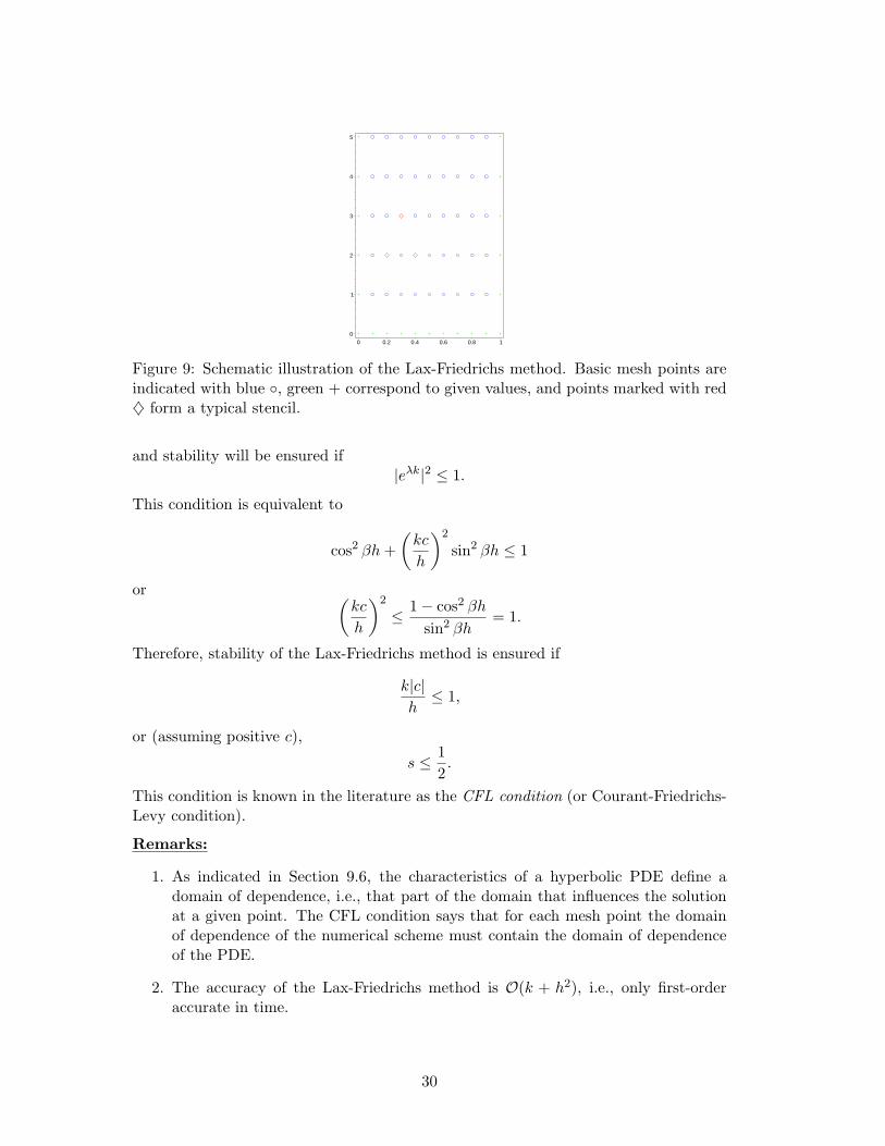
Figure 9: Schematic illustration of the Lax-Friedrichs method. Basic mesh points areindicated with blue , green + correspond to given values, and points marked with red♦ form a typical stencil.
and stability will be ensured if|eλk|2 ≤ 1.
This condition is equivalent to
cos2 βh +(
kc
h
)2
sin2 βh ≤ 1
or (kc
h
)2
≤ 1− cos2 βh
sin2 βh= 1.
Therefore, stability of the Lax-Friedrichs method is ensured if
k|c|h
≤ 1,
or (assuming positive c),
s ≤ 12.
This condition is known in the literature as the CFL condition (or Courant-Friedrichs-Levy condition).
Remarks:
1. As indicated in Section 9.6, the characteristics of a hyperbolic PDE define adomain of dependence, i.e., that part of the domain that influences the solutionat a given point. The CFL condition says that for each mesh point the domainof dependence of the numerical scheme must contain the domain of dependenceof the PDE.
2. The accuracy of the Lax-Friedrichs method is O(k + h2), i.e., only first-orderaccurate in time.
30
3. We use the Matlab program transport.m (with menu option ”Lax-Friedrichs”)on the advection equation with a smooth step function as initial condition toillustrate the performance of this method.
We now present an alternate interpretation of the Lax-Friedrichs method. To thisend we rewrite (46). By subtracting the term vi,j from both sides of (46) we get
vi,j+1 − vi,j
k= −c
[vi+1,j − vi−1,j
2h
]+
12
[vi+1,j − 2vi,j + vi−1,j
k
]. (47)
We can now interpret (47) as a finite difference discretization of the PDE
ut(x, t) = −cux(x, t) +h2
2kuxx(x, t)
using symmetric approximation for the space derivatives, and a forward difference intime.
According to this interpretation we have implicitly added a diffusion term to theadvection equation. This process is referred to as adding numerical viscosity (or ar-tificial viscosity) to a hyperbolic problem. By doing so we introduce stability in thenumerical method, but destroy its conservation properties. The effect is that sharpdiscontinuites in the solution (shocks) are smeared out.
The diffusive effect of the Lax-Friedrichs method can also be observed by lookingat the amplification factor. Since
|eλk|2
= 1, |c|k = h,< 1, |c|k < h,
the amplitude of the wave decreases, i.e., energy is lost, if the time step is taken toosmall.
Remark: For certain hyperbolic problems the diffusive effect is not much of an issuesince for those problems one is interested in the case when βh 1, so that |eλk| ≈ 1.
Lax-Wendroff MethodWe now present another finite difference scheme for conservation laws named after
Peter Lax and Burt Wendroff. We start with the Taylor expansion
u(x, t + k) = u(x, t) + kut(x, t) +k2
2utt(x, t) + . . . .
Using the conservation equation ut = −cux this becomes
u(x, t + k) = u(x, t)− ckux(x, t) +(ck)2
2uxx(x, t) + . . . .
If we keep the terms explicitly listed, then the truncation error in the time componentobviously is O(k2).
With the standard notation vi,j = u(xi, tj) this expansion gives rise to the numericalscheme
vi,j+1 = vi,j − ckvi+1,j − vi−1,j
2h+
(ck)2
2vi+1,j − 2vi,j + vi−1,j
h2,
31
where we have used O(h2) approximations for both the first-order and second-orderspatial derivatives. Therefore, introducing the mesh ratio s = ck
2h we get the Lax-Wendroff method
vi,j+1 =(2s2 − s
)vi+1,j +
(1− 4s2
)vi,j +
(2s2 + s
)vi−1,j . (48)
This method enjoys O(k2 + h2) accuracy, is an explicit method, and involves a stencilas shown in Figure 10.
0
1
2
3
4
5
0 0.2 0.4 0.6 0.8 1
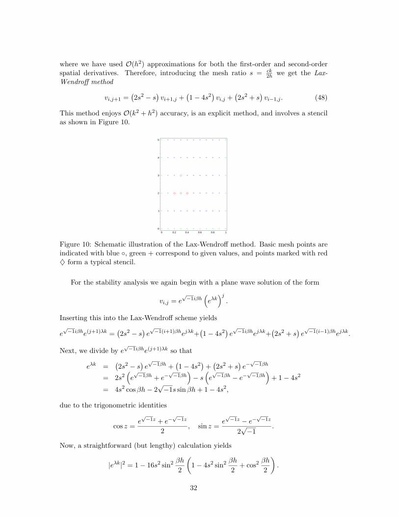
Figure 10: Schematic illustration of the Lax-Wendroff method. Basic mesh points areindicated with blue , green + correspond to given values, and points marked with red♦ form a typical stencil.
For the stability analysis we again begin with a plane wave solution of the form
vi,j = e√−1iβh
(eλk
)j.
Inserting this into the Lax-Wendroff scheme yields
e√−1iβhe(j+1)λk =
(2s2 − s
)e√−1(i+1)βhejλk+
(1− 4s2
)e√−1iβhejλk+
(2s2 + s
)e√−1(i−1)βhejλk.
Next, we divide by e√−1iβhe(j+1)λk so that
eλk =(2s2 − s
)e√−1βh +
(1− 4s2
)+
(2s2 + s
)e−√−1βh
= 2s2(e√−1βh + e−
√−1βh
)− s
(e√−1βh − e−
√−1βh
)+ 1− 4s2
= 4s2 cos βh− 2√−1s sinβh + 1− 4s2,
due to the trigonometric identities
cos z =e√−1z + e−
√−1z
2, sin z =
e√−1z − e−
√−1z
2√−1
.
Now, a straightforward (but lengthy) calculation yields
|eλk|2 = 1− 16s2 sin2 βh
2
(1− 4s2 sin2 βh
2+ cos2
βh
2
).
32
Stability will be ensured if the term in parentheses is non-negative, i.e.,
1− 4s2 sin2 βh
2+ cos2
βh
2≥ 0.
It is easy to show that the expression on the left-hand side takes its minimum forβh = π
2 . The minimum value is then 1− 4s2, and it will be nonnegative as long as
|s| ≤ 12.
This is the CFL condition encountered earlier.
Remark: We use the Matlab program transport.m (with menu option ”Lax-Wendroff”)on the advection equation with a smooth step function as initial condition to illustratethe performance of this method.
Leapfrog Method
Another method that is second-order accurate in time and space for the advectionequation can be found by using symmetric approximations to the partial derivatives,i.e.,
vi,j+1 − vi,j−1
2k= −c
vi+1,j − vi−1,j
2hor
vi,j+1 = −ck
h[vi+1,j − vi−1,j ] + vi,j−1. (49)
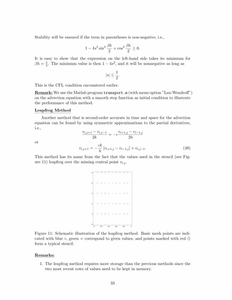
This method has its name from the fact that the values used in the stencil (see Fig-ure 11) leapfrog over the missing central point vi,j .
0
1
2
3
4
5
0 0.2 0.4 0.6 0.8 1
Figure 11: Schematic illustration of the leapfrog method. Basic mesh points are indi-cated with blue , green + correspond to given values, and points marked with red ♦form a typical stencil.
Remarks:
1. The leapfrog method requires more storage than the previous methods since thetwo most recent rows of values need to be kept in memory.
33
2. Also, this method requires a special start-up step (which may be of lower order).
The stability analysis of the leapfrog method involves the solution of a quadraticequation, and leads to the amplification factor
eλk = −√−1
ck
hsinβh±
√1−
(ck
h
)2
sin2 βh
so that
|eλk|2 =(
ck
h
)2
sin2 βh + 1−(
ck
h
)2
sin2 βh
= 1.
Therefore, the leapfrog method is stable for our model problem for all mesh ratioss = ck
2h , and does not involve any numerical diffusivity.However, for more complicated (nonlinear) problems this method becomes unstable.
This instability is due to the fact that the stencil isolates the ”black” from the ”white”mesh points. This leads to so-called mesh drifting.
Remark: By combining the leapfrog method with the Lax-Friedrichs method it ispossible to get a two-step Lax-Wendroff type method which has accuracy O(k2 + h2)and is stable (i.e., does not suffer from mesh drifting).
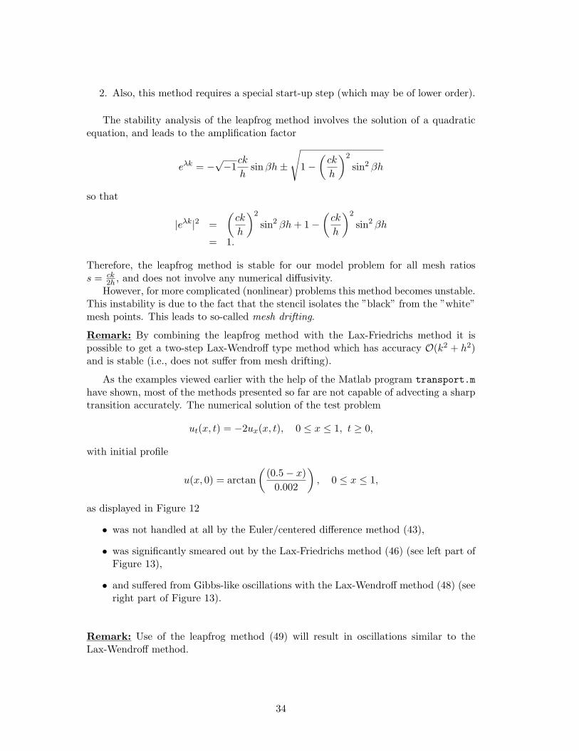
As the examples viewed earlier with the help of the Matlab program transport.mhave shown, most of the methods presented so far are not capable of advecting a sharptransition accurately. The numerical solution of the test problem
ut(x, t) = −2ux(x, t), 0 ≤ x ≤ 1, t ≥ 0,
with initial profile
u(x, 0) = arctan(
(0.5− x)0.002
), 0 ≤ x ≤ 1,
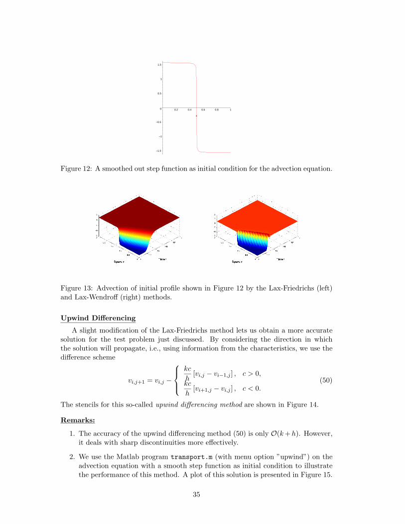
as displayed in Figure 12
• was not handled at all by the Euler/centered difference method (43),
• was significantly smeared out by the Lax-Friedrichs method (46) (see left part ofFigure 13),
• and suffered from Gibbs-like oscillations with the Lax-Wendroff method (48) (seeright part of Figure 13).
Remark: Use of the leapfrog method (49) will result in oscillations similar to theLax-Wendroff method.
34
–1.5
–1
–0.5
0
0.5
1
1.5
0.2 0.4 0.6 0.8 1
x
Figure 12: A smoothed out step function as initial condition for the advection equation.
Figure 13: Advection of initial profile shown in Figure 12 by the Lax-Friedrichs (left)and Lax-Wendroff (right) methods.
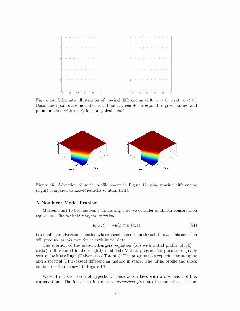
Upwind Differencing
A slight modification of the Lax-Friedrichs method lets us obtain a more accuratesolution for the test problem just discussed. By considering the direction in whichthe solution will propagate, i.e., using information from the characteristics, we use thedifference scheme
vi,j+1 = vi,j −
kc
h[vi,j − vi−1,j ] , c > 0,
kc
h[vi+1,j − vi,j ] , c < 0.
(50)
The stencils for this so-called upwind differencing method are shown in Figure 14.
Remarks:
1. The accuracy of the upwind differencing method (50) is only O(k +h). However,it deals with sharp discontinuities more effectively.
2. We use the Matlab program transport.m (with menu option ”upwind”) on theadvection equation with a smooth step function as initial condition to illustratethe performance of this method. A plot of this solution is presented in Figure 15.
35
0
1
2
3
4
5
0 0.2 0.4 0.6 0.8 10
1
2
3
4
5
0 0.2 0.4 0.6 0.8 1
Figure 14: Schematic illustration of upwind differencing (left: c > 0, right: c < 0).Basic mesh points are indicated with blue , green + correspond to given values, andpoints marked with red ♦ form a typical stencil.
Figure 15: Advection of initial profile shown in Figure 12 using upwind differencing(right) compared to Lax-Friedrichs solution (left).
A Nonlinear Model Problem
Matters start to become really interesting once we consider nonlinear conservationequations. The inviscid Burgers’ equation
ut(x, t) = −u(x, t)ux(x, t) (51)
is a nonlinear advection equation whose speed depends on the solution u. This equationwill produce shocks even for smooth initial data.
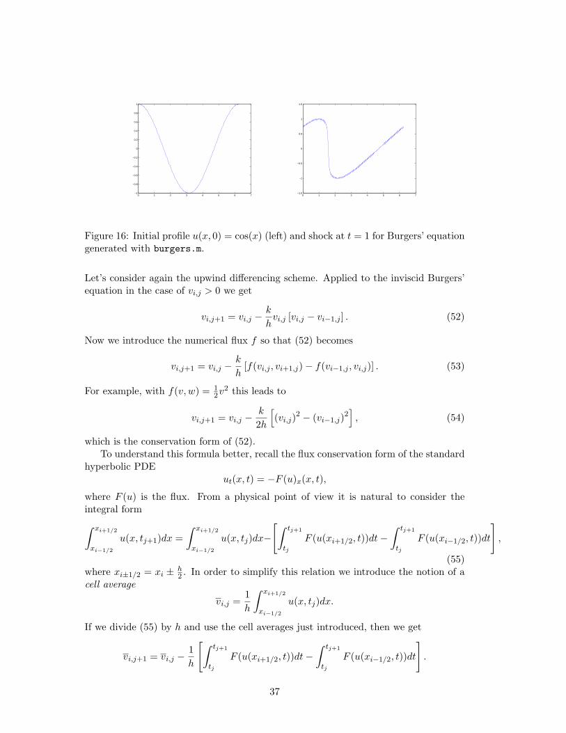
The solution of the inviscid Burgers’ equation (51) with initial profile u(x, 0) =cos(x) is illustrated in the (slightly modified) Matlab program burgers.m originallywritten by Mary Pugh (University of Toronto). The program uses explicit time-steppingand a spectral (FFT-based) differencing method in space. The initial profile and shockat time t = 1 are shown in Figure 16.
We end our discussion of hyperbolic conservation laws with a discussion of fluxconservation. The idea is to introduce a numerical flux into the numerical scheme.
36
0 1 2 3 4 5 6 7−1
−0.8
−0.6
−0.4
−0.2
0
0.2
0.4
0.6
0.8
1
0 1 2 3 4 5 6 7−1.5
−1
−0.5
0
0.5
1
1.5
Figure 16: Initial profile u(x, 0) = cos(x) (left) and shock at t = 1 for Burgers’ equationgenerated with burgers.m.
Let’s consider again the upwind differencing scheme. Applied to the inviscid Burgers’equation in the case of vi,j > 0 we get
vi,j+1 = vi,j −k
hvi,j [vi,j − vi−1,j ] . (52)
Now we introduce the numerical flux f so that (52) becomes
vi,j+1 = vi,j −k
h[f(vi,j , vi+1,j)− f(vi−1,j , vi,j)] . (53)
For example, with f(v, w) = 12v2 this leads to
vi,j+1 = vi,j −k
2h
[(vi,j)
2 − (vi−1,j)2], (54)
which is the conservation form of (52).To understand this formula better, recall the flux conservation form of the standard
hyperbolic PDEut(x, t) = −F (u)x(x, t),
where F (u) is the flux. From a physical point of view it is natural to consider theintegral form∫ xi+1/2
xi−1/2
u(x, tj+1)dx =∫ xi+1/2
xi−1/2
u(x, tj)dx−
[∫ tj+1
tj
F (u(xi+1/2, t))dt−∫ tj+1
tj
F (u(xi−1/2, t))dt
],
(55)where xi±1/2 = xi ± h
2 . In order to simplify this relation we introduce the notion of acell average
vi,j =1h
∫ xi+1/2
xi−1/2
u(x, tj)dx.
If we divide (55) by h and use the cell averages just introduced, then we get
vi,j+1 = vi,j −1h
[∫ tj+1
tj
F (u(xi+1/2, t))dt−∫ tj+1
tj
F (u(xi−1/2, t))dt
].
37
Finally, using a numerical flux defined as a time-average of the true flux, i.e.,
f(vi,j , vi+1,j) =1k
∫ tj+1
tj
F (u(xi+1/2, t)dt,
we get
vi,j+1 = vi,j −k
h[f(vi,j , vi+1,j)− f(vi−1,j , vi,j)] .
Therefore, vi,j in (53) can be interpreted as an approximation to the cell average
vi,j =1h
∫ xi+1/2
xi−1/2
u(x, tj)dx.
Remarks:
1. State-of-the-art methods for solving hyperbolic conservation laws are the finitevolume methods described in the book ”Finite Volume Methods for HyperbolicProblems” by Randy LeVeque (2002), and also featured in the software libraryCLAW.
2. An alternative are so-called essentially non-oscillating (ENO) methods introducedby Stan Osher, Chi-Wang Shu, and others. These methods are based on theintegral form of the conservation law, and use polynomial interpolation on smallstencils that are chosen so that the developing shock is preserved.
3. The full (viscous) Burgers’ equation
ut(x, t) = −u(x, t)ux(x, t) +1R
uxx(x, t)
with Reynolds number R is much easier to solve numerically than the inviscidequation (51). This is due to the smoothing effect of the diffusive term uxx. Onlyfor large Reynolds numbers does this equation resemble the inviscid case, andbecomes a challenge for numerical methods.
4. All of the methods discussed above can be generalized to systems of conservationlaws.
9.8 Other Methods for Time-Dependent PDEs
Method of Lines
The method of lines is a semi-discrete method. The main idea of this method isto convert the given PDE to a system of ODEs. This is done by discretizing in space,and leaving the time variable continuous. Thus, we will end up with a system of ODEinitial value problems that can be attacked with standard solvers.
If, e.g., we want to solve the heat equation
ut(x, t) = uxx(x, t)
38
with zero boundary temperature and initial temperature u(x, 0) = f(x), then we candiscretize this problem in space only (using a second-order accurate symmetric differ-ence approximation). This means that on each line through a spatial mesh point inx0, x1, . . . , xn we have the ODE
dui
dt(t) =
ui+1(t)− 2ui(t) + ui−1(t)h2
, i = 1, . . . , n− 1, (56)
with boundary and initial conditions
u0(t) = un(t) = 0, ui(0) = f(xi).
In matrix form we haveu′(t) = Au(t),
where, for this example, the matrix A is given by
A =1h2
−2 1 0 . . . 0
1 −2 1...
0. . . . . . . . . 0
... 1 −2 10 . . . 0 1 −2
,
and u = [u1, . . . , un − 1]T . Any standard IVP solver can be used to solve this system.However, for small h this matrix is very stiff, and so some care has to be taken inchoosing the solver.Remark: From (56) it is apparent that we are obtaining the solution of the wave equa-tion along lines with constant x-value (parallel to the time-axis). This interpretationhas given the method its name.
(Pseudo-)Spectral Methods
Another semi-discrete approach involves an expansion in terms of basis functionsfor the spatial part of the PDE, and an IVP solver for the time component.
Assume that the numerical solution is given in the form
uh(x, t) =n∑
j=1
cj(t)φj(x),
where the φj form a basis for an approximation space used for the space component.Ideally, these basis functions will satisfy the boundary conditions of the PDE. Thetime-dependent coefficients cj can be determined via collocation at a discrete set ofpoints x1, . . . , xn. If we again use the heat equation
ut(x, t) = uxx(x, t)
to illustrate this method, then the collocation conditions are
∂uh
∂t(xi, t) =
∂2uh
∂x2(xi, t), i = 1, . . . , n,
39
orn∑
j=1
c′j(t)φj(xi) =n∑
j=1
cj(t)φ′′j (xi), i = 1, . . . , n.
This is a system of n first-order ODEs for the coefficients cj . In matrix form we have
Ac′(t) = Bc(t), (57)
where c = [c1, . . . , cn]T and the matrices A and B have entries
Aij = φj(xi), Bij = φ′′j (xi).
The initial conditions for (57) can be obtained by interpolation
n∑j=1
cj(0)φj(xi) = f(xi),
where f specifies the initial condition of the PDE.
Remarks:
1. Standard IVP solvers can be used to solve the system (57). Of course, the basisfunctions should be such that the matrix A is invertible.
2. All standard interpolation or approximation methods can be used to generate thebasis φ1, . . . , φn (e.g., polynomials, splines, radial basis functions).
3. Again, the ODE systems (57) are often rather stiff, which means that the IVPsolvers need to be chosen carefully.
4. The program burgers.m used earlier employs a trigonometric basis coupled withthe fast Fourier transform, and leapfrog time-stepping for ODEs (initialized withone forward Euler step).
Time-Dependent Galerkin Methods
It is also possible to combine the basis function expansion with a least squares bestapproximation criterion instead of collocation as indicated in Section 9.4. This leadsto time-dependent Galerkin methods.
Assume that the numerical solution is given in the form
uh(x, t) =n∑
j=1
cj(t)φj(x), (58)
where the φj form a basis for an approximation space used for the space component. Tokeep the discussion simple, we will assume that the basis functions satisfy the boundaryconditions of the PDE. We will once more use the heat equation
ut(x, t) = uxx(x, t)
40
with boundary conditions u(0, t) = u(1, t) = 0 and initial condition u(x, 0) = f(x) toillustrate this method. Inserting the expansion (58) into the heat equation results in
n∑j=1
c′j(t)φj(x) =n∑
j=1
cj(t)φ′′j (x). (59)
The conditions for the time-dependent coefficients cj are generated by taking innerproducts of (59) with the basis functions φi, i = 1, . . . , n. This results in a system of nfirst-order ODEs for the coefficients cj of the form
n∑j=1
c′j(t)〈φj , φi〉 =n∑
j=1
cj(t)〈φ′′j , φi〉,
where the inner products are standard L2-inner products over the spatial domain (as-sumed to be [0, 1] here)
〈v, w〉 =∫ 1
0v(x)w(x)dx.
In matrix form we haveAc′(t) = Bc(t), (60)
where c = [c1, . . . , cn]T and the matrices A and B have entries
Aij = 〈φj , φi〉, Bij = 〈φ′′j , φi〉.
If the basis functions are orthogonal on [0, 1] then the matrix A is diagonal, and thesystem (60) is particularly simple to solve.
As for the spectral methods above, the initial condition becomesn∑
j=1
cj(0)φj(x) = f(x),
and the initial coefficients cj(0), j = 1, . . . , n, can be obtained by interpolation orleast squares approximation. In the case of least squares approximation (with orthog-onal basis functions) the coefficients are given by the generalized Fourier coefficientscj(0) = 〈f, φi〉.
By applying integration by parts to the entries of B (remember that the basisfunctions are assumed to satisfy the boundary conditions) we get an equivalent system
Ac′(t) = −Cc(t)
with ”stiffness matrix” C with entries
Cij = [φj , φi] =∫ 1
0φ′j(x)φ′i(x)dx.
This is analogous to the inner product in the Ritz-Galerkin method of Section 9.4.
Remarks:
1. Higher-dimensional time-dependent PDEs can be attacked by using higher-dimensionalspatial methods, such as finite elements, or higher-dimensional collocation schemes.
2. Matlab’s pdetool.m uses piecewise linear finite elements in a Galerkin methodto solve both (linear) parabolic and hyperbolic PDEs.
41