Numerical Solutions to Partial Differential Equations

Abhishek Mukherjee, Pun Cheuk Nga Janice,Mateusz Jakub Staniszewski and Seongguk Ryou

Supervised by Professor Grigoris Pavliotis

June 2016

AbstractFrom the famous Navier-Stokes equation which finds a variety of applications in engineering whilst alsobeing of interest to pure mathematicians, to the Black-Scholes equation which arises in finance and op-tions pricing, partial differential equations (PDEs) govern our universe at every level. In most practicalcases, it is not possible to solve these equations analytically. This project gives an introduction to somenumerical methods which can be used to estimate solutions to PDEs and provides a more in-depth anal-ysis of spectral methods with some specific linear and non-linear examples.

In the first part of the project, an introduction to partial differential equations and various examples aregiven according to their classification, followed by an overview of the Finite Differences and Finite Ele-ments methods for solving PDEs.

In the next section, spectral method are introduced with examples including linear PDEs such as theHeat, Wave, and Poisson equations and non-linear ones such as Inviscid Burgers’ and Korteweg-deVries’ equations.

In the final part, the advantages and disadvantages of using Spectral Methods are discussed. Additionallyall results are summarised and we examine areas for further analysis of these partial differential equa-tions.

Keywords: numerical solutions, spectral methods, basis functions, exact solutions

1

Contents

1 Background 3

2 Introduction to Partial Differential Equations 42.1 Examples of PDEs . . . . . . . . . . . . . . . . . . . . . . . . . . . . . . . . . . . . . . . 42.2 Analytical Solution to Laplace’s Equation . . . . . . . . . . . . . . . . . . . . . . . . . . . 5

3 Method I: Finite Differences 63.1 Deriving Formula using Taylor Expansion . . . . . . . . . . . . . . . . . . . . . . . . . . . 63.2 Introducing Mesh Grid Notation . . . . . . . . . . . . . . . . . . . . . . . . . . . . . . . . 73.3 Heat Equation . . . . . . . . . . . . . . . . . . . . . . . . . . . . . . . . . . . . . . . . . . 7

4 Method II: Finite Elements 104.1 Overview . . . . . . . . . . . . . . . . . . . . . . . . . . . . . . . . . . . . . . . . . . . . 104.2 Historical background . . . . . . . . . . . . . . . . . . . . . . . . . . . . . . . . . . . . . . 104.3 Finite Element Method Example . . . . . . . . . . . . . . . . . . . . . . . . . . . . . . . . 11

5 Method III: Spectral Methods 145.1 Fourier Spectral Method . . . . . . . . . . . . . . . . . . . . . . . . . . . . . . . . . . . . 145.2 Chebyshev Fourier Spectral Method . . . . . . . . . . . . . . . . . . . . . . . . . . . . . . 155.3 Spectral Accuracy . . . . . . . . . . . . . . . . . . . . . . . . . . . . . . . . . . . . . . . . 16

6 Solving Partial Differential Equations 186.1 Linear . . . . . . . . . . . . . . . . . . . . . . . . . . . . . . . . . . . . . . . . . . . . . . 18

6.1.1 Wave Equation . . . . . . . . . . . . . . . . . . . . . . . . . . . . . . . . . . . . . 186.1.2 Heat Equation . . . . . . . . . . . . . . . . . . . . . . . . . . . . . . . . . . . . . . 196.1.3 Poisson Equation . . . . . . . . . . . . . . . . . . . . . . . . . . . . . . . . . . . . 21

6.2 Non-Linear Equations . . . . . . . . . . . . . . . . . . . . . . . . . . . . . . . . . . . . . . 246.2.1 Inviscid Burgers’ Equation . . . . . . . . . . . . . . . . . . . . . . . . . . . . . . . 246.2.2 Korteweg-de Vries Equation . . . . . . . . . . . . . . . . . . . . . . . . . . . . . . 27

7 Conclusion 30

8 Appendix 31

2

1 Background

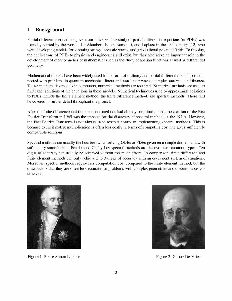
Partial differential equations govern our universe. The study of partial differential equations (or PDEs) wasformally started by the works of d’Alembert, Euler, Bernoulli, and Laplace in the 18th century [12] whowere developing models for vibrating strings, acoustic waves, and gravitational potential fields. To this day,the applications of PDEs to physics and engineering still exist, but they also serve an important role in thedevelopment of other branches of mathematics such as the study of abelian functions as well as differentialgeometry.

Mathematical models have been widely used in the form of ordinary and partial differential equations con-nected with problems in quantum mechanics, linear and non-linear waves, complex analysis, and finance.To use mathematics models in computers, numerical methods are required. Numerical methods are used tofind exact solutions of the equations in these models. Numerical techniques used to approximate solutionsto PDEs include the finite element method, the finite difference method, and spectral methods. These willbe covered in further detail throughout the project.

After the finite difference and finite element methods had already been introduced, the creation of the FastFourier Transform in 1965 was the impetus for the discovery of spectral methods in the 1970s. However,the Fast Fourier Transform is not always used when it comes to implementing spectral methods. This isbecause explicit matrix multiplication is often less costly in terms of computing cost and gives sufficientlycomparable solutions.

Spectral methods are usually the best tool when solving ODEs or PDEs given on a simple domain and withsufficiently smooth data. Fourier and Chebyshev spectral methods are the two most common types. Tendigits of accuracy can usually be achieved without too much effort. In comparison, finite difference andfinite element methods can only achieve 2 to 3 digits of accuracy with an equivalent system of equations.Moreover, spectral methods require less computation cost compared to the finite element method, but thedrawback is that they are often less accurate for problems with complex geometries and discontinuous co-efficients.

Figure 1: Pierre-Simon Laplace Figure 2: Gustav De-Vries

3

2 Introduction to Partial Differential Equations

2.1 Examples of PDEs

A partial differential equation is an equation involving functions of a particular variable and their partialderivatives. Partial differential equations are generally more difficult to solve analytically than ordinarydifferential equations. Thankfully, they can be solved by methods such as separation of variable, using aGreen’s Function, or numerical methods.

Example of PDEs:

1. Linear equations

(a) Laplace’s Equation:∆u =

∑ni=1 uxixi = 0

(b) Helmoholtz’s equation:−∆u = λu

(c) Heat (or diffusion Equation)ut −∆u = 0

(d) Wave Equationutt −∆u = 0

(e) Schrodinger’s Equationiut + ∆u− 0

(f) Beam equationutt + uxxxx = 0

2. Non− linear Equations

(a) Scalar reaction-diffusion equationut −∆u = f(u)

(b) Non-linear Poisson Equation−∆u = f(u)

(c) Inviscid Burgers’ Equationut + uux = 0

(d) Non-linear Wave Equationutt −∆u+ f(u) = 0

(e) Korteweg-de Vries Equationut + uux + uxxx = 0

Second order linear PDEs can be formally classified into three types including elliptic, parabolic and hyper-bolic. We can write any second order PDE in the form Auxx + 2Buxy + Cuyy + lower order terms = 0and define the classifications as follows.

1. Elliptic (if B2 −AC < 0)e.g Poisson Equation or Laplace equation (whenf(x, y) = 0)Uxx + Uyy = f(x, y)

2. Parabolic (if B2 −AC = 0)e.g Diffusion equationUt = kUxx

3. Hyperbolic (if B2 −AC > 0)e.g Wave EquationUtt = c2Uxx

4

2.2 Analytical Solution to Laplace’s Equation

Though it is not the primary focus of this paper, it is important to note that it’s possible to solve PDEswithout even requiring the use of numerical methods. Take, for example, Laplace’s equation

∇2Φ = 0.

Re-expressing in polar co-ordinates [8], this can be written as

1

r

∂

∂r

(r∂Φ

∂r

)+

1

r2

∂2Φ

∂θ2= 0.

Consider solutions of the form Φ(r, θ) = R(r)Θ(θ) to use separation of variables and solve it analytically.Substituting this in gives

Θ

r

d

dr

(rdR

dr

)+R

r2

d2Θ

dθ2= 0

=⇒ r

R

d

dr

(rdR

dr

)= −Θ′′

Θ= λ.

Because we have separated the variables, both sides must be equal to a constant λ. Focusing on Θ

Θ′′ = −λΘ

=⇒ Θ =

Acos

√λθ +B sin

√λθ if λ 6= 0

A+B θ if λ = 0

Given that∇Θ is 2π periodic, we can rewrite this as

Θ =

Acos nθ +B sinnθ if n 6= 0

A+Bθ if n = 0

Switching our attention to R, we can use the substitution u = ln r to get

R =

Crn +Dr−n if n 6= 0

C +D ln r if n = 0

Combining the solutions for R and Θ gives

RΘ =

(Crn +Dr−n)(Acos nθ +B sinnθ) if n 6= 0

(C +D ln r)(A+Bθ) if n = 0

As we are dealing with a linear Partial Differential Equation we can express a general solution as a combi-nation of all possible solutions

Φ = A0 +B0θ + C0 ln r +

∞∑n=1

(Anrn + Cnr

−n) cos nθ +

∞∑n=1

(Bnrn +Dnr

−n) sin nθ.

We can eliminate the θ ln r solution as it does not satisfy the requirement that ∇Θ is 2π periodic. We alsorelabel the constants such that AC = An, AD = Cn, BC = Bn, and BD = Dn. This expression couldbe simplified = even further, but the above expression is the most practical form. Then, given boundaryconditions, we can work our specific solutions.

5

3 Method I: Finite Differences

3.1 Deriving Formula using Taylor Expansion

This part of the project will give an introduction to the finite difference method of solving partial differentialequations, and an example of solving the heat equation in one space dimension will be presented underDirichlet boundary conditions. Error and stability will also be briefly discussed.

In this method, the partial differential equations are replaced by a set of equations, using an associated gridsystem [2]. The derivatives are approximated by algebraic equations - to perform the analysis we shall findsuch expressions for:

∂u(x, y)

∂x,∂2u(x, y)

∂y2,∂2u(x, y)

∂x2,∂2u(x, y)

∂y2

First consider Taylor expansions of u(x, y), keeping t constant:

u(x+ h, y) = u(x, y) + h∂u(x, y)

∂x+h2

2!

∂2u(x, y)

∂x2+h3

3!

∂3u(x, y)

∂x3+ . . . (3.1)

u(x− h, y) = u(x, y)− h∂u(x, y)

∂x+h2

2!

∂2u(x, y)

∂x2− h3

3!

∂3u(x, y)

∂x3+ . . . (3.2)

Adding equations (3.1) and (3.2) and rearranging for ∂u(x,y)∂x we obtain:

∂u(x, y)

∂x=u(x+ h, y) + u(x− h, y)

2h+O(h2) (3.3)

This is known as the central difference approximation. Directly from equations (3.1) and (3.2) we can alsoobtain the forward and backward difference approximations:

∂u(x, y)

∂x=u(x+ h, y)− u(x, y)

h+O(h) (3.4)

∂u(x, y)

∂x=u(x, y)− u(x− h, y)

h+O(h) (3.5)

The remainder O(h), is known as the local truncation error and will be discussed in a later part of this sec-tion. Similarly, it will be useful to derive the second order partial derivative being (summing and rearranging(3.1) and (3.2)):

∂2u(x, y)

∂x2=u(x+ h, y) + u(x− h, y)− 2u(x, y)

h2+O(h2) (3.6)

Respective approximations can be obtained for partial derivatives with respect to time (denoting the smallincrement of time δ(y) by k).

6

3.2 Introducing Mesh Grid Notation

For further analysis of partial differential equations, the following grid shall be introduced:

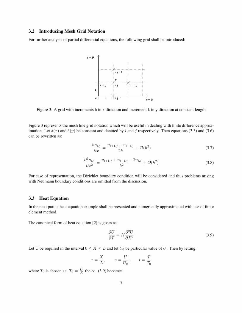
Figure 3: A grid with increments h in x direction and increment k in y direction at constant length

Figure 3 represents the mesh line grid notation which will be useful in dealing with finite difference approx-imation. Let δ(x) and δ(y) be constant and denoted by i and j respectively. Then equations (3.3) and (3.6)can be rewritten as:

∂ui,j∂x

=ui+1,j − ui−1,j

2h+O(h2) (3.7)

∂2ui,j∂x2

=ui+1,j + ui−1,j − 2ui,j

h2+O(h2) (3.8)

For ease of representation, the Dirichlet boundary condition will be considered and thus problems arisingwith Neumann boundary conditions are omitted from the discussion.

3.3 Heat Equation

In the next part, a heat equation example shall be presented and numerically approximated with use of finiteelement method.

The canonical form of heat equation [2] is given as:

∂U

∂T= K

∂2U

∂X2(3.9)

Let U be required in the interval 0 ≤ X ≤ L and let U0 be particular value of U . Then by letting:

x =X

L, u =

U

U0, t =

T

T0

where T0 is chosen s.t. T0 = L2

K the eq. (3.9) becomes:

7

∂u

∂t=∂2u

∂x2where 0 ≤ x ≤ 1 (3.10)

By substituting the forward difference approximation (eq. (3.4)) for the LHS of equation (3.10) and thecentral difference approximation (eq. (3.8)) for the RHS, in the mesh grid notation we obtain:

ui+1,j − ui−1,j

k=ui+1,j + ui−1,j − 2ui,j

h2(3.11)

Notice that that the truncation errors are of different orders and appears reasonable to set k = O(h2). Alsothe equation is consistent (local truncation error tends to 0) as when:

limh→∞,k→∞

O(k + h2) = 0 (3.12)

In practice we need to choose values for h and k. Here two types of errors shall be noted [3]:

1. Truncation error: due to approximation of derivative - reduced by choosing smaller values of h and k

2. Roundoff error: due to computer rounding at every calculation - reduced by choosing greater valuesof h and k

Additionally to ensure the solution of (3.11) to be stable we need [3]:

r =k

h2≤ 1

2(3.13)

With this knowledge, an attempt to solve a specific example of the heat equation will be made to explicitlyshow the finite difference method (this is done with the explicit method). Equation (3.11) can be rewrittenas:

ui,j+1 = ui,j + r(ui−1,j − 2ui,j + ui+1,j) (3.14)

Consider equation (3.10) with conditions:

(i) u(0, t) = u(0, L) = 0 Boundary condition

(ii) u(x, 0) = sin(x) Initial condition

Using the fact that L = 2π due to periodic solution, the Matlab code is used (can be found in Appendix),giving the following graphical solution:

8

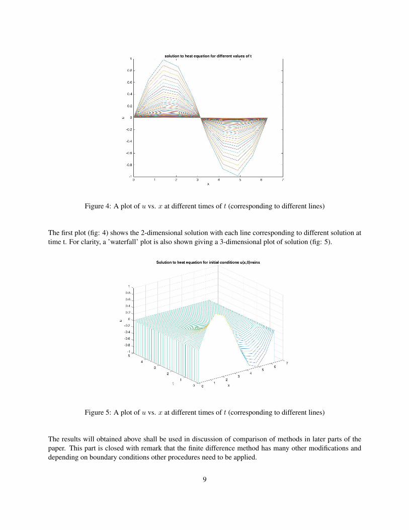
Figure 4: A plot of u vs. x at different times of t (corresponding to different lines)

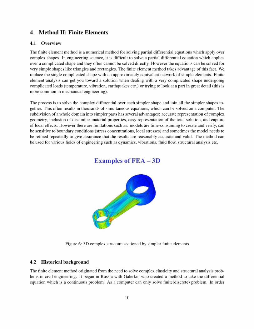
The first plot (fig: 4) shows the 2-dimensional solution with each line corresponding to different solution attime t. For clarity, a ’waterfall’ plot is also shown giving a 3-dimensional plot of solution (fig: 5).

Figure 5: A plot of u vs. x at different times of t (corresponding to different lines)

The results will obtained above shall be used in discussion of comparison of methods in later parts of thepaper. This part is closed with remark that the finite difference method has many other modifications anddepending on boundary conditions other procedures need to be applied.

9

4 Method II: Finite Elements

4.1 Overview

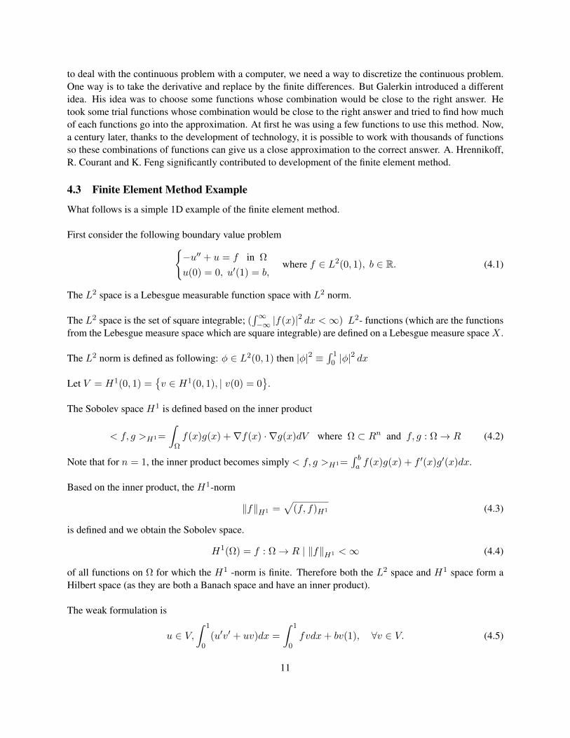
The finite element method is a numerical method for solving partial differential equations which apply overcomplex shapes. In engineering science, it is difficult to solve a partial differential equation which appliesover a complicated shape and they often cannot be solved directly. However the equations can be solved forvery simple shapes like triangles and rectangles. The finite element method takes advantage of this fact. Wereplace the single complicated shape with an approximately equivalent network of simple elements. Finiteelement analysis can get you toward a solution when dealing with a very complicated shape undergoingcomplicated loads (temperature, vibration, earthquakes etc.) or trying to look at a part in great detail (this ismore common in mechanical engineering).

The process is to solve the complex differential over each simpler shape and join all the simpler shapes to-gether. This often results in thousands of simultaneous equations, which can be solved on a computer. Thesubdivision of a whole domain into simpler parts has several advantages: accurate representation of complexgeometry, inclusion of dissimilar material properties, easy representation of the total solution, and captureof local effects. However there are limitations such as: models are time-consuming to create and verify, canbe sensitive to boundary conditions (stress concentrations, local stresses) and sometimes the model needs tobe refined repeatedly to give assurance that the results are reasonably accurate and valid. The method canbe used for various fields of engineering such as dynamics, vibrations, fluid flow, structural analysis etc.

Figure 6: 3D complex structure sectioned by simpler finite elements

4.2 Historical background

The finite element method originated from the need to solve complex elasticity and structural analysis prob-lems in civil engineering. It began in Russia with Galerkin who created a method to take the differentialequation which is a continuous problem. As a computer can only solve finite(discrete) problem. In order

10

to deal with the continuous problem with a computer, we need a way to discretize the continuous problem.One way is to take the derivative and replace by the finite differences. But Galerkin introduced a differentidea. His idea was to choose some functions whose combination would be close to the right answer. Hetook some trial functions whose combination would be close to the right answer and tried to find how muchof each functions go into the approximation. At first he was using a few functions to use this method. Now,a century later, thanks to the development of technology, it is possible to work with thousands of functionsso these combinations of functions can give us a close approximation to the correct answer. A. Hrennikoff,R. Courant and K. Feng significantly contributed to development of the finite element method.

4.3 Finite Element Method Example

What follows is a simple 1D example of the finite element method.

First consider the following boundary value problem−u′′ + u = f in Ω

u(0) = 0, u′(1) = b,where f ∈ L2(0, 1), b ∈ R. (4.1)

The L2 space is a Lebesgue measurable function space with L2 norm.

The L2 space is the set of square integrable; (∫∞−∞ |f(x)|2 dx <∞) L2- functions (which are the functions

from the Lebesgue measure space which are square integrable) are defined on a Lebesgue measure spaceX .

The L2 norm is defined as following: φ ∈ L2(0, 1) then |φ|2 ≡∫ 1

0 |φ|2 dx

Let V = H1(0, 1) =v ∈ H1(0, 1), | v(0) = 0

.

The Sobolev space H1 is defined based on the inner product

< f, g >H1=

∫Ωf(x)g(x) +∇f(x) · ∇g(x)dV where Ω ⊂ Rn and f, g : Ω→ R (4.2)

Note that for n = 1, the inner product becomes simply < f, g >H1=∫ ba f(x)g(x) + f ′(x)g′(x)dx.

Based on the inner product, the H1-norm

‖f‖H1 =√

(f, f)H1 (4.3)

is defined and we obtain the Sobolev space.

H1(Ω) = f : Ω→ R | ‖f‖H1 <∞ (4.4)

of all functions on Ω for which the H1 -norm is finite. Therefore both the L2 space and H1 space form aHilbert space (as they are both a Banach space and have an inner product).

The weak formulation is

u ∈ V,∫ 1

0(u′v′ + uv)dx =

∫ 1

0fvdx+ bv(1), ∀v ∈ V. (4.5)

11

Existence of an unique solution is guaranteed by the Lax-Milgram Lemma which will be followed shortlybut before we go into that, there are two things which need to be defined: bilinears form and coercivefunctions.The bilinear form on a vector space V is defined as a function B : V × V → K which is linear in eachargument separately:

B(u+ v, w) = B(u,w) +B(v, w)

B(u, v + w) = B(u, v) +B(u,w)

B(λu, v) = B(u, λv) = λB(u, v).

A bilinear function φ on a normed space E is called coercive if there exists a positive constant K such thatφ(x, x) ≥ K ‖x‖2 ∀x ∈ E.

Let φ be a bounded coercive bilinear form on a Hilbert space H . The Lax-Milgram theorem states that,for every bounded linear functional f on H , there exists a unique xj ∈ H such that f(x) = φ(x, xf ).

Now partition the domain I = [0, 1] into N parts as 0 = x0 < x1 < · · · < xN = 1. We call thepoints xi, 0 6 i 6 N nodes. The sub-intervals Ii = [xi−1, xi], 1 6 i 6 N are called elements. Denotehi = xi − xi−1 and the mesh parameter h = max1≤i≤Nhi

An approximate solution will be sought in the space Vh = vh ∈ V | vh | Ii ∈ P1(Ii), 1 ≤ i ≤ N Giventhe properties of the Sobolev space H1(I), we also have vh ∈ C(I)

Now we choose the basis functions as following:

For i = 1, · · · , N − 1:

φi(x) =

(x− xi−1)/hi, xi−1 ≤ x ≤ xi,(xi+1 − x)/hi+1, xi ≤ x ≤ xi+1,

0, otherwise

(4.6)

For i = N :

φN (x) =

(x− xN−1)/hN , xN−1 ≤ x ≤ xN ,0, otherwise

(4.7)

The defined basis functions are linearly independent and we have Vh =spanφi, 1 ≤ i ≤ N, so their weakderivatives exist. They are defined almost everywhere and are equal to constants. Hence our finite elementmethod becomes:

uh ∈ Vh,∫ 1

0(u′hv

′h + uhvh)dx =

∫ 1

0fvhdx+ bvh(1), ∀vh ∈ Vh (4.8)

which, using the representation uh =∑N

i=1 ujφj , can be transformed to the linear system

N∑i=1

uj

∫ 1

0(φ′iφ

′j + φiφj)dx =

∫ 1

0fφidx+ bφi(1), 1 ≤ i ≤ N (4.9)

12

This system can be written as Au = b, whereu = (u1, . . . , uN )T is the vector of unknown coefficientsb = (

∫ 10 fφidx, . . . ,

∫ 10 fφN−1dx,

∫ 10 fφNdx+ b)T is the load vector

We can form a stiffness matrix which represents the system of linear equations that must be solved in orderto calculate an approximate solution to the differential equation. Entries of the stiffness matrix can becalculated as Aij =

∫ 10 (φ′iφ

′j + φiφj)dx using the formulae

∫ 1

0φ′iφ′i−1dx = −1

h, 2 ≤ i ≤ N,

∫ 1

0(φ′i)

2dx =2

h, 1 ≤ i ≤ N − 1,∫ 1

0φiφi−1dx =

h

6, 2 ≤ i ≤ N,

∫ 1

0(φi)

2dx =2h

3, 1 ≤ i ≤ N − 1∫ 1

0(φ′N )2dx =

1

h,

∫ 1

0(φN )2dx =

h

3

From above, we can obtain the stiffness matrix

A =

(2h

3 + 2h) (h6 + 1

h)

(h6 + 1h) (2h

3 + 2h) (h6 + 1

h). . . . . . . . .

(h6 + 1h) (2h

3 + 2h) (h6 + 1

h)

(h6 + 1h) (h3 + 1

h)

(4.10)

By solving Au = b,where A is the stiffness matrix and b is the load vector, the process ends.

In summary, the finite element method can be derived in such steps.

1. Discretise domain

2. Derive (simpler) finite element equations

3. Assemble and combine element equations

4. Apply boundary constraints

5. Solve

6. Post-processing (visualisation)

13

5 Method III: Spectral Methods

By taking the differentiation matrix produced through a finite difference model and taking the process to thelimit by using a differentiation formula of infinite order and bandwidth, we end up with a spectral method.In practice, we cannot work with infinite matrices, so the approach is to:

1. Define a function f s.t. f(xj) = uj for every j

2. Let wj = f ′(xj)

In general we can split simple problems by examining the domain type. For periodic domains, it is usuallymost appropriate to create a basis using trigonometric polynomials on an equispaced grid. For non-periodicdomains, we use algebraic polynomials e.g Chebyshev polynomial on irregular grids.

5.1 Fourier Spectral Method

For a periodic domain, we usually use the Fourier spectral method to calculate the numerical solution ofPDEs. First we use our fundamental spatial domain [−π, π) and let n be a positive even integer,

h =2π

n

Define xj = jh. The grid points in this domain are

x−n2

= −π, ..., x0 = 0, ..., xn2−1 = π − h

Then take the discrete Fourier transform:

vk = h

n2−1∑

j=−n2

e−ikjhvj

Take the Inverse discrete Fourier Transform:

vj =1

2π

n2−1∑

j=−n2

e−ikjhvk

As a result, we can calculate a numerical solution for the partial equation. However the implementation ofthe spectral method does not always use the fast Fourier transform in the process. Instead, explicit matrixmultiplication may be used to calculate numerical solution of PDEs in order to reduce computational cost.It can be done by setting up matrix interpolating using the sinc function, Chebyshev function etc. Then wecan derive a set of linear equations to find the numerical result. An example using such a method will alsobe shown later on.

14

5.2 Chebyshev Fourier Spectral Method

The Chebyshev spectral method can be implemented by using the fast Fourier transform method. In somecases, the Chebyshev spectral method can be used to speed up the calculation.

Domain of Chebyshev series:

Chebyshev series in x ∈ [−1, 1]

The Chebyshev polynomial denoted Tn is defined by

Tn(x) = cos(ncos−1x) = cosnθ for x = cosθ

In general

Tn+1(x) =1

2(zn+1 + z−n+1) =

1

2(zn + z−n)(z + z−1)− 1

2(zn−1 + z1−n)

Recurrence relations can be set up

Tn+1(x) = 2xTn(x)− Tn−1(x)

As Tn(x) has exactly n degrees for every n and any polynomial with degree n can be denoted as

p(x) =N∑n=0

anTn(x) x ∈ [−1, 1]

p(x) =N∑n=0

ancosnθ θ ∈ R

Steps for Chebyshev spectral method:

1. Given data v0, ..., vn at Chebyshev points x0 = 1, ..xn = −1. Represent the data by a vector V oflength 2N where V2n−j = vj , j = 1, 2, ..., n− 1

2. Using the fast Fourier transform,

Vk = πn

∑2nj=1 e

−ikθj , k = −n+ 1, ..., n

3. Define Wk = ikVk except Wn = 0

4. Compute the derivative of the trigonometric interpolant P on the equispaced grid by the inverse FFT

Wj = 12π

∑n−n+1 e

ikθjWk j = 1, ..., 2n

5. Calculate the derivative of the algebraic polynomial p on the interior grid points

p(x) = P (θ) where x = cosθ

p′(x) = P ′(θ)dx/dθ =

−∑n

n=0 nansinnθ

−(1−x2)12

= −P ′(θ)√1−x2

15

wj = − Wj√1−x2 j = 1, ..., n− 1

with the special formulas for the end points

w0 = 12π

∑n′i=0 i

2vn wn = 12π

∑n′i=0(−1)i+1i2vn

The Chebyshev spectral method can be used to calculate PDEs with boundary conditions. In some case,using a Chebyshev grid can reach higher accuracy than an equispaced grid.

5.3 Spectral Accuracy

One of the primary reasons for using spectral methods is due to their accuracy when compared to the finitemethods. This property is known as spectral accuracy, and is due to the fast that smooth functions haverapidly decaying Fourier transforms. As a result, the aliasing errors that arise as a result of discretisationare relatively small. In general, as N increases, convergence at the rate O(N−m) is achieved as long as thesolution is infinitely differentiable.

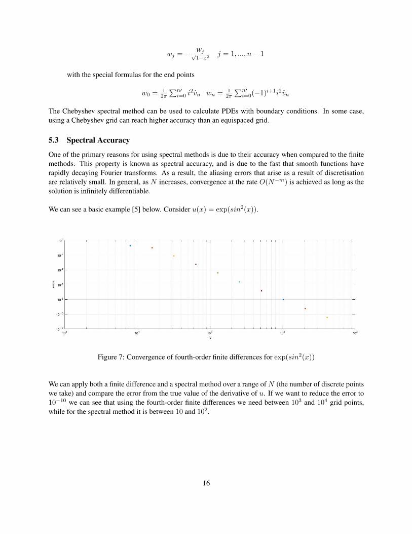
We can see a basic example [5] below. Consider u(x) = exp(sin2(x)).

Figure 7: Convergence of fourth-order finite differences for exp(sin2(x))

We can apply both a finite difference and a spectral method over a range of N (the number of discrete pointswe take) and compare the error from the true value of the derivative of u. If we want to reduce the error to10−10 we can see that using the fourth-order finite differences we need between 103 and 104 grid points,while for the spectral method it is between 10 and 102.

16

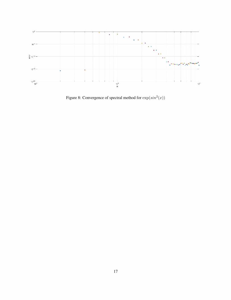
Figure 8: Convergence of spectral method for exp(sin2(x))

17

6 Solving Partial Differential Equations

In the following section, linear and non-linear examples will be solved using spectral methods. For the timedependence, finite difference methods such as the leap-frog and Euler time-step method will be used.

6.1 Linear

6.1.1 Wave Equation

Waves are everywhere. Most of the information that we receive comes to us in the form of waves. Wavestransfer energy in different forms and the discovery of the wave equation by d’Alembert has had a significantcontribution to the engineering field.

The wave equation is the important partial differential equation that describes propagation of waves withspeed v.

∇2ψ =1

v2

∂2ψ

∂t2(6.1)

The form above gives the wave equation in three-dimensional space where ∇2 is the Laplacian, which canalso be written v2∇2ψ = ψtt. Now we will show how the solution of the wave equation would look usingspectral method on MATLAB.

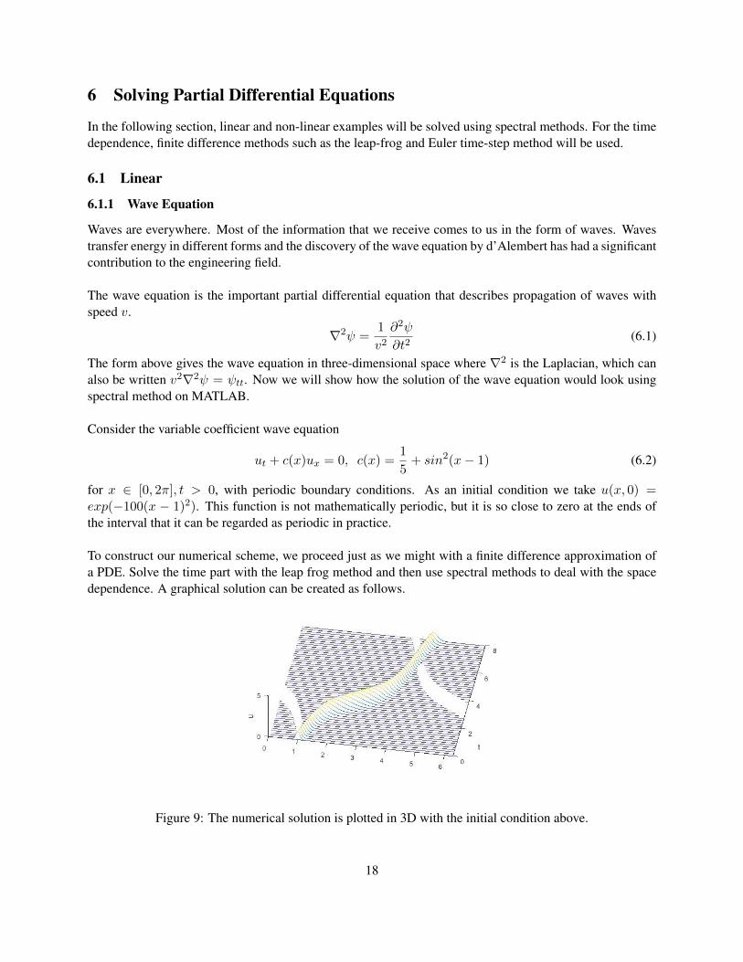
Consider the variable coefficient wave equation

ut + c(x)ux = 0, c(x) =1

5+ sin2(x− 1) (6.2)

for x ∈ [0, 2π], t > 0, with periodic boundary conditions. As an initial condition we take u(x, 0) =exp(−100(x − 1)2). This function is not mathematically periodic, but it is so close to zero at the ends ofthe interval that it can be regarded as periodic in practice.

To construct our numerical scheme, we proceed just as we might with a finite difference approximation ofa PDE. Solve the time part with the leap frog method and then use spectral methods to deal with the spacedependence. A graphical solution can be created as follows.

Figure 9: The numerical solution is plotted in 3D with the initial condition above.

18

6.1.2 Heat Equation

The Heat equation describes the distribution of temperature in a period of time for some object. It is oneof the most common and discussed partial differential equations. An example of the heat equation wouldinclude a rod of metal bar and the distribution of temperature inside it. Various assumptions can be madebut most commonly it’s said that the bar is insulated on the lateral surface and temperature can only escapeon either of the ends of the bar. A heat equation belongs to class of parabolic linear equations and is oftenwritten in the form:

∂U

∂T= K∆U (6.3)

As shown in section 3 the equation (6.3) can be transformed to simplified form, which will be dealt withusing spectral methods:

∂u

∂t= ∆u (6.4)

with pre-defined initial condition:

u(x, 0) = u0(x) (6.5)

Then there are 3 distinct types of boundary conditions which are considered for partial differential equations[9]. Let Ω denote the bounded domain in Rn (note that we are dealing with heat equation in n dimensions).Then the following conditions may be considered:

1. Dirichlet Boundary Condition:

u = 0 on δΩ

2. Neumann Boundary Condition:

∂u

∂v= 0 on δΩ

3. Robin Boundary Condition:

αu+ β∂u

∂v= 0 α, β > 0

To show how to tackle the heat equation in this section we will use 1-dimensional heat equation with Dirich-let Boundary Condition and initial condition u(x, 0) = sin(x) - thus the problem we shall consider takesform:

∂u

∂t=∂2u

∂x2(6.6)

u(x, 0) = sin(x) initial condition

u(0, t) = u(0, L) = 0 boundary condition

By taking the Fourier transform in x we can rewrite above equation by:

19

∂u

∂t= k

∂2u

∂2t

We use the hat symbol to denote a partial derivative’s Fourier transform. For the Fourier transform of u in xfollowing equation is obtained:

∂mu(ω, t)

∂xm= (iω)mu(ω, t)

Thus:

∂u

∂t= k(iω)2u(ω, t) (6.7)

Using the Forward Euler-Method on equation (6.7) it can be written in the form:

ui,j+1 = ui,j + kh(iω)2ui,j (6.8)

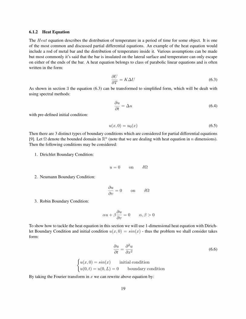
Here h denotes time-step and the reader can see the resemblance to the finite difference method for solvingthe heat equation. All that is left is the visual representation which will be done by MATLAB code [13].Upon running the code following visual representation of numerical solution is obtained:

Figure 10: The numerical solution of u(x, t) is plotted in 3D

The resemblance to the solution in section 3 is straightforward. By modifying the code it’s easy to checksolutions for other initial conditions, with periodic boundary problem. i.e. for:

∂u

∂t=∂2u

∂x2(6.9)

20

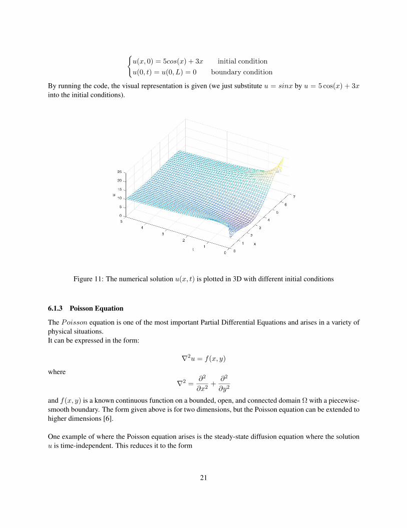
u(x, 0) = 5cos(x) + 3x initial condition

u(0, t) = u(0, L) = 0 boundary condition

By running the code, the visual representation is given (we just substitute u = sinx by u = 5 cos(x) + 3xinto the initial conditions).

Figure 11: The numerical solution u(x, t) is plotted in 3D with different initial conditions

6.1.3 Poisson Equation

The Poisson equation is one of the most important Partial Differential Equations and arises in a variety ofphysical situations.It can be expressed in the form:

∇2u = f(x, y)

where

∇2 =∂2

∂x2+

∂2

∂y2

and f(x, y) is a known continuous function on a bounded, open, and connected domain Ω with a piecewise-smooth boundary. The form given above is for two dimensions, but the Poisson equation can be extended tohigher dimensions [6].

One example of where the Poisson equation arises is the steady-state diffusion equation where the solutionu is time-independent. This reduces it to the form

21

∇2u = 0 (6.10)

which is Laplace’s equation, a special case of the Poisson equation that was solved analytically in Section2. Similar examples also exist in electrostatics and gravitation.

To be able to solve the Poisson equation we require boundary conditions. Having an initial condition doesnot make sense. For the purposes of computation, we will work with Dirichlet conditions, i.e.

u(x, y) = g(x, y), (x, y) ∈ ∂Ω

where g is a function defined on the boundary of Ω.

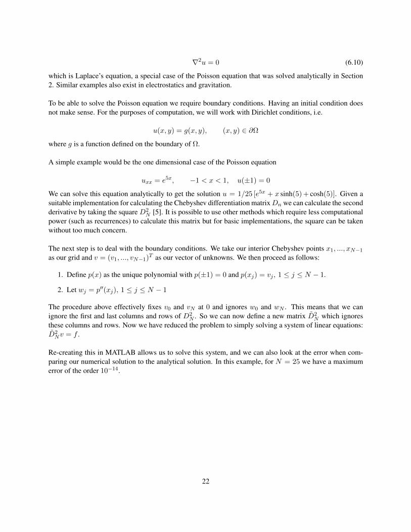
A simple example would be the one dimensional case of the Poisson equation

uxx = e5x, −1 < x < 1, u(±1) = 0

We can solve this equation analytically to get the solution u = 1/25 [e5x + x sinh(5) + cosh(5)]. Given asuitable implementation for calculating the Chebyshev differentiation matrixDn we can calculate the secondderivative by taking the square D2

N [5]. It is possible to use other methods which require less computationalpower (such as recurrences) to calculate this matrix but for basic implementations, the square can be takenwithout too much concern.

The next step is to deal with the boundary conditions. We take our interior Chebyshev points x1, ..., xN−1

as our grid and v = (v1, ..., vN−1)T as our vector of unknowns. We then proceed as follows:

1. Define p(x) as the unique polynomial with p(±1) = 0 and p(xj) = vj , 1 ≤ j ≤ N − 1.

2. Let wj = p′′(xj), 1 ≤ j ≤ N − 1

The procedure above effectively fixes v0 and vN at 0 and ignores w0 and wN . This means that we canignore the first and last columns and rows of D2

N . So we can now define a new matrix D2N which ignores

these columns and rows. Now we have reduced the problem to simply solving a system of linear equations:D2Nv = f .

Re-creating this in MATLAB allows us to solve this system, and we can also look at the error when com-paring our numerical solution to the analytical solution. In this example, for N = 25 we have a maximumerror of the order 10−14.

22

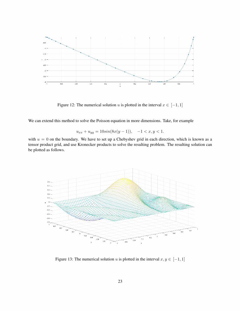
Figure 12: The numerical solution u is plotted in the interval x ∈ [−1, 1]

We can extend this method to solve the Poisson equation in more dimensions. Take, for example

uxx + uyy = 10sin(8x(y − 1)), −1 < x, y < 1.

with u = 0 on the boundary. We have to set up a Chebyshev grid in each direction, which is known as atensor product grid, and use Kronecker products to solve the resulting problem. The resulting solution canbe plotted as follows.

Figure 13: The numerical solution u is plotted in the interval x, y ∈ [−1, 1]

23

6.2 Non-Linear Equations

In this section we calculate some numerical solutions to partial differential equations with non-linear terms.

6.2.1 Inviscid Burgers’ Equation

A partial differential equation of the form ut+(f(u))x = 0 is called a conservation law in which u representthe density of some quantity and f(u) associate rightward flux. Integrating with respect to t,

d

dt

∫ b

au(x)dx = f(u(a, t))− f(u(b, t))

A non-linear example of the conservation law is the Inviscid Burgers’ equation. It is a first order quasilinearhyperbolic equation. The equation has the form:

∂u

∂t+ u

∂u

∂x= 0

This equation can be used in gas dynamics and traffic flows. One crucial phenomenon that arises by theInviscid Burgers equation is the formation shock which is discontinuity happens after a certain finite timepropagating in a regular manner.

Example of inviscid Burger’s equation:Shock Wave with periodic domain

∂u

∂t+ u

∂u

∂x= 0 0 ≤ x ≤ 2π

with initial conditions:

u(x, 0) = f(x) = exp(−10(4x− 1)2)

u(x, t) = f(x− ut)

Note: Constant wave speed =1 (wave travel at a maximum wave speed u=1) m, wave speed depends onu(x, t).

24

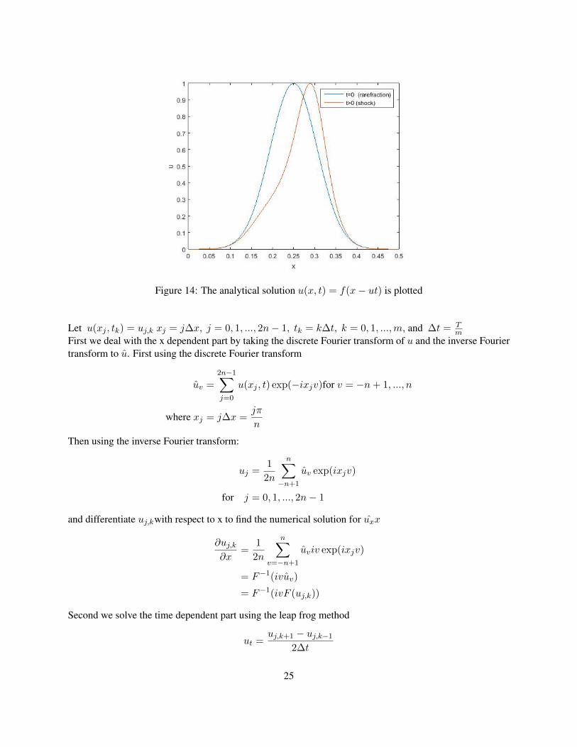
Figure 14: The analytical solution u(x, t) = f(x− ut) is plotted

Let u(xj , tk) = uj,k xj = j∆x, j = 0, 1, ..., 2n− 1, tk = k∆t, k = 0, 1, ...,m, and ∆t = Tm

First we deal with the x dependent part by taking the discrete Fourier transform of u and the inverse Fouriertransform to u. First using the discrete Fourier transform

uv =

2n−1∑j=0

u(xj , t) exp(−ixjv)for v = −n+ 1, ..., n

where xj = j∆x =jπ

n

Then using the inverse Fourier transform:

uj =1

2n

n∑−n+1

uv exp(ixjv)

for j = 0, 1, ..., 2n− 1

and differentiate uj,kwith respect to x to find the numerical solution for uxx

∂uj,k∂x

=1

2n

n∑v=−n+1

uviv exp(ixjv)

= F−1(ivuv)

= F−1(ivF (uj,k))

Second we solve the time dependent part using the leap frog method

ut =uj,k+1 − uj,k−1

2∆t

25

From the equation,

ut + uux = 0

uj,k+1 = uj,k−1 − 2∆t uj,k F−1(ivF (uj,k))

Assume wave speed u ≈ 1, set t = −∆t

uj,−1 = u(x,−∆t) = u(x+ 1*∆t) = f(x− ut)≈ f(x+ ∆t) = exp(−10(4(x+ ∆t− 1)2)

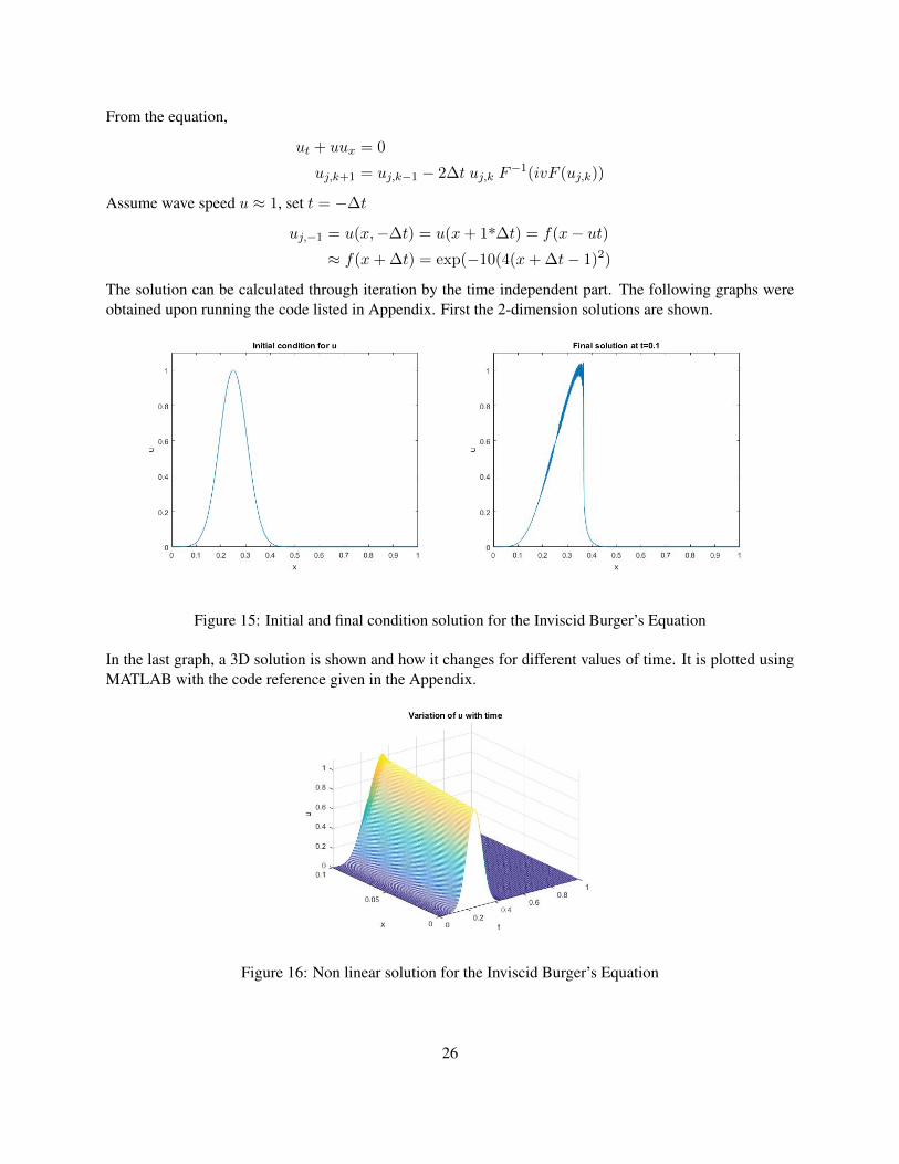
The solution can be calculated through iteration by the time independent part. The following graphs wereobtained upon running the code listed in Appendix. First the 2-dimension solutions are shown.

Figure 15: Initial and final condition solution for the Inviscid Burger’s Equation

In the last graph, a 3D solution is shown and how it changes for different values of time. It is plotted usingMATLAB with the code reference given in the Appendix.

Figure 16: Non linear solution for the Inviscid Burger’s Equation

26

6.2.2 Korteweg-de Vries Equation

The Korteweg-de Vries Equation was discovered by a phenomenon observed by a young Scottish engineernamed John Scott Russell (1808-1882). He observed solitary waves (waves of translation) in the UnionCanal at Hermiston which is closed to Riccarton campus of Heriot-Watt University Edinburgh.His ideas was not recognised until the mid 1960s when applied scientists began to use modern digital com-puters to calculate nonlinear wave propagation. He viewed the solitary wave as a self-sufficient dynamicentity, a ”thing” displaying many properties of a particle.The phenomenon described by Russell can be expressed by a non-linear partial differentiation equation ofthird order as shown below:

∂u∂t + εu∂u∂x + ∂3u

∂x3= 0

The Korteweg-de Vries Equation was derived by Korteweg-de Vries (1985) which describe a non-linearshallow water wave. It is a hyperbolic partial differentiation equation as illustrated in section 2.

1. Solitons waves are result from solution of kdV

2. Non linear term causes waves to steepen: ux

3. Dispersive term cause waves to disperse uxxx

Example of Korteweg-de Vries Equation: We will calculate a solution using a Fourier spectral method:

∂u

∂t+ u

∂u

∂x+∂3u

∂x3= 0 0 ≤ x ≤ 2π (6.11)

with periodic boundary conditions u(0) = u(2π)Initial condition:

u(x, 0) = A sech2(

√A

12(x− π − A

3t)) A = 100

First, we deal with the x dependent part of u using the fast Fourier transform. Take the discrete Fouriertransform of u

uv =2n−1∑j=0

u(xj , t) exp(−ixjv) for v = −n+ 1, ..., n

where xj = j∆x =jπ

n

Then we take the inverse Fourier Transform:

uj =1

2n

n∑−n+1

uv exp(ixjv)

for j = 0, 1, ..., 2n− 1

and differentiate uj,kwith respect to x in order to find the numerical solution ux

∂uj,k∂x

=1

2n

n∑v=−n+1

uviv exp(ixjv)

= F−1(ivF (uj,k))

27

Find uxxx using the same method as above

uxxx =∂3uj,k∂x3

=1

2n

n∑v=−n+1

uv exp(ixjv)

= F−1(iv3F (uj,k))

Second, we deal with the time dependent part of u using the leap frog method

ut =uj,k+1 − uj,k−1

2∆t

uj,k+1 = uj,k−1 + 2∆t( uj,k F−1(ivF (uj,k)) + F−1((iv)3F (uj,k))

In order to remove instability for high wave number, uxxx is approximate as below:

sin(v3∆t) ≈ v3∆t+O(∆t3)

as ∆t→ 0Therefore it is a good approximation Using sinx = x− x3

3! + ... we get

uj,k+1 = uj,k−1 + 2∆t( uj,k F−1(ivF (uj,k)) + F−1(−i sin(v3∆t)F (uj,k))

which is a stable solution.

Another method to remove instability is to use an integrating factor. It is based on the idea that the non-linearpart can be transformed to the linear part of the partial equation. From (6.11) Take Fourier Transform:

ut +i

2ku2 − ik3u = 0

Multiply it with eik3t

eik3tut + eik

3t i

2ku2 − ik3eik

3tu = 0

Define U = eik3tu with Ut = ik3U + eik

3tut It becomes

Ut + ik3U +i

2eik

3tku2 − ik3U = 0

Ut +i

2eik

3tku2 = 0

which is a linear partial differentiation equation.

Continue using the first method by approximate using Taylor seriesGiven wave speed u = A

3 , set t = −∆t

28

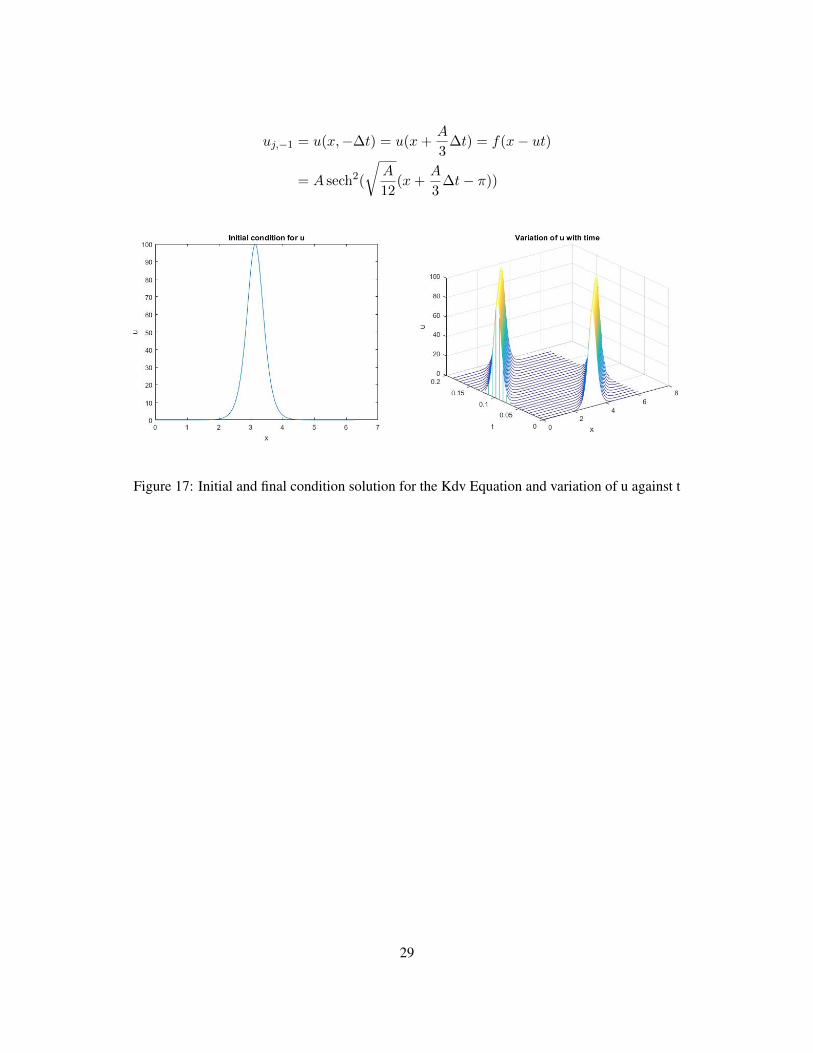
uj,−1 = u(x,−∆t) = u(x+A

3∆t) = f(x− ut)

= A sech2(

√A

12(x+

A

3∆t− π))

Figure 17: Initial and final condition solution for the Kdv Equation and variation of u against t

29

7 Conclusion

Partial differential equations can be used to describe a wide variety of phenomena such as sound, heat, elec-trostatics, electrodynamics, fluid flow, elasticity, quantum mechanics and even the stock market.

Numerical methods have made solving partial differential equations significantly easier. Sometimes, par-tial differential equations are difficult to solve analytically. The introduction of numerical methods is asignificant achievement that allows people to find numerical solution of partial differential equation usingcomputers.

In the above, we have shown three major numerical methods to solve partial differentiation equations in-cluding finite element, finite difference and spectral methods. We also have shown several famous examplesof solving partial differentiation equations using the Fourier spectral method and Chebyshev differentiationmatrix.

To compare between the three methods, spectral methods have a lot of advantages over the finite differenceand finite element methods. Firstly, spectral methods have higher accuracy on smooth functions, achieving10 digits of accuracy for a relatively small number of grid points. Secondly, spectral methods usually havea higher efficiency. They require less computation time, hence saving cost in calculating problems. Finally,they can achieve exponential convergence/spectral convergence as shown in previous sections.

However, spectral methods also suffers drawbacks. Firstly, programming spectral models is relatively moredifficult when compared to using the finite difference method. It has to be divided into two methods to solvethe time dependent and space dependent equations. Secondly, it is more costly per degree of freedom thanthe finite difference method. In geometries for especially complicated domains, the spectral method heavilyloses its accuracy.

To continue our study, solving numerical solution using spectral method in rectangular grid and polar co-ordinate can be done. Moreover, instead of solving equation using the Fourier spectral method, we can tryto solving equation using collocation and Tau spectral methods. More complicated equations can also becomputed using spectral methods. In addition, we could also look at modern implementations of the finitedifference method and finite element method. Last, a modified spectral method could also be investigated totry and overcome disadvantages of spectral methods.

30

8 Appendix

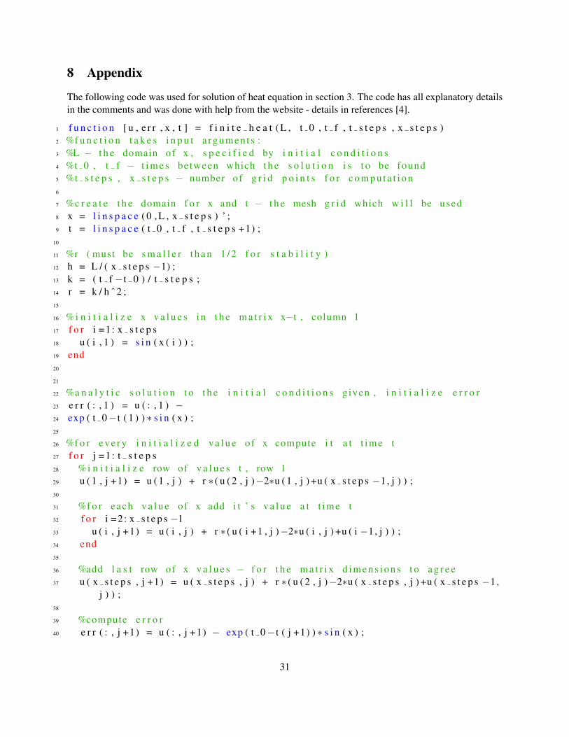
The following code was used for solution of heat equation in section 3. The code has all explanatory detailsin the comments and was done with help from the website - details in references [4].

1 f u n c t i o n [ u , e r r , x , t ] = f i n i t e h e a t ( L , t 0 , t f , t s t e p s , x s t e p s )2 %f u n c t i o n t a k e s i n p u t a rgumen t s :3 %L − t h e domain o f x , s p e c i f i e d by i n i t i a l c o n d i t i o n s4 %t 0 , t f − t i m e s between which t h e s o l u t i o n i s t o be found5 %t s t e p s , x s t e p s − number o f g r i d p o i n t s f o r c o m p u t a t i o n6

7 %c r e a t e t h e domain f o r x and t − t h e mesh g r i d which w i l l be used8 x = l i n s p a c e ( 0 , L , x s t e p s ) ’ ;9 t = l i n s p a c e ( t 0 , t f , t s t e p s +1) ;

10

11 %r ( must be s m a l l e r t h a n 1 / 2 f o r s t a b i l i t y )12 h = L / ( x s t e p s −1) ;13 k = ( t f −t 0 ) / t s t e p s ;14 r = k / h ˆ 2 ;15

16 %i n i t i a l i z e x v a l u e s i n t h e m a t r i x x−t , column 117 f o r i =1 : x s t e p s18 u ( i , 1 ) = s i n ( x ( i ) ) ;19 end20

21

22 %a n a l y t i c s o l u t i o n t o t h e i n i t i a l c o n d i t i o n s g iven , i n i t i a l i z e e r r o r23 e r r ( : , 1 ) = u ( : , 1 ) −24 exp ( t 0−t ( 1 ) ) ∗ s i n ( x ) ;25

26 %f o r e v e r y i n i t i a l i z e d v a l u e o f x compute i t a t t ime t27 f o r j =1 : t s t e p s28 %i n i t i a l i z e row of v a l u e s t , row 129 u ( 1 , j +1) = u ( 1 , j ) + r ∗ ( u ( 2 , j )−2∗u ( 1 , j ) +u ( x s t e p s −1, j ) ) ;30

31 %f o r each v a l u e o f x add i t ’ s v a l u e a t t ime t32 f o r i =2 : x s t e p s −133 u ( i , j +1) = u ( i , j ) + r ∗ ( u ( i +1 , j )−2∗u ( i , j ) +u ( i −1, j ) ) ;34 end35

36 %add l a s t row of x v a l u e s − f o r t h e m a t r i x d i m e n s i o n s t o a g r e e37 u ( x s t e p s , j +1) = u ( x s t e p s , j ) + r ∗ ( u ( 2 , j )−2∗u ( x s t e p s , j ) +u ( x s t e p s −1,

j ) ) ;38

39 %compute e r r o r40 e r r ( : , j +1) = u ( : , j +1) − exp ( t 0−t ( j +1) ) ∗ s i n ( x ) ;

31

41 end42

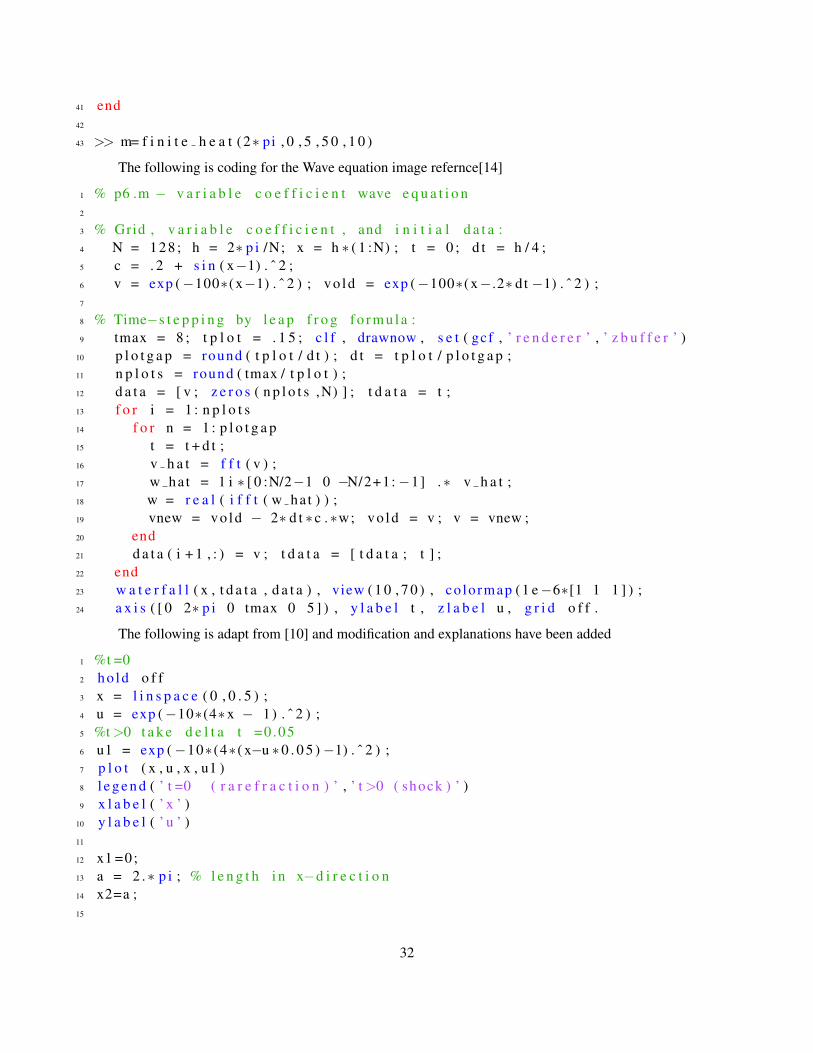
43 >> m= f i n i t e h e a t (2∗ pi , 0 , 5 , 5 0 , 1 0 )

The following is coding for the Wave equation image refernce[14]

1 % p6 .m − v a r i a b l e c o e f f i c i e n t wave e q u a t i o n2

3 % Grid , v a r i a b l e c o e f f i c i e n t , and i n i t i a l d a t a :4 N = 128 ; h = 2∗ p i /N; x = h ∗ ( 1 :N) ; t = 0 ; d t = h / 4 ;5 c = . 2 + s i n ( x−1) . ˆ 2 ;6 v = exp (−100∗(x−1) . ˆ 2 ) ; vo ld = exp (−100∗(x−.2∗ dt −1) . ˆ 2 ) ;7

8 % Time−s t e p p i n g by l e a p f r o g f o r m u l a :9 tmax = 8 ; t p l o t = . 1 5 ; c l f , drawnow , s e t ( gcf , ’ r e n d e r e r ’ , ’ z b u f f e r ’ )

10 p l o t g a p = round ( t p l o t / d t ) ; d t = t p l o t / p l o t g a p ;11 n p l o t s = round ( tmax / t p l o t ) ;12 d a t a = [ v ; z e r o s ( n p l o t s ,N) ] ; t d a t a = t ;13 f o r i = 1 : n p l o t s14 f o r n = 1 : p l o t g a p15 t = t + d t ;16 v h a t = f f t ( v ) ;17 w hat = 1 i ∗ [ 0 :N/2−1 0 −N/2+1:−1] .∗ v h a t ;18 w = r e a l ( i f f t ( w ha t ) ) ;19 vnew = vo ld − 2∗ d t ∗c .∗w; vo ld = v ; v = vnew ;20 end21 d a t a ( i + 1 , : ) = v ; t d a t a = [ t d a t a ; t ] ;22 end23 w a t e r f a l l ( x , t d a t a , d a t a ) , view ( 1 0 , 7 0 ) , co lormap (1 e−6∗[1 1 1 ] ) ;24 a x i s ( [ 0 2∗ p i 0 tmax 0 5 ] ) , y l a b e l t , z l a b e l u , g r i d o f f .

The following is adapt from [10] and modification and explanations have been added

1 %t =02 ho ld o f f3 x = l i n s p a c e ( 0 , 0 . 5 ) ;4 u = exp (−10∗(4∗x − 1) . ˆ 2 ) ;5 %t>0 t a k e d e l t a t =0 .056 u1 = exp (−10∗ (4∗ ( x−u ∗0 . 0 5 )−1) . ˆ 2 ) ;7 p l o t ( x , u , x , u1 )8 l e g e n d ( ’ t =0 ( r a r e f r a c t i o n ) ’ , ’ t>0 ( shock ) ’ )9 x l a b e l ( ’ x ’ )

10 y l a b e l ( ’ u ’ )11

12 x1 =0;13 a = 2 .∗ p i ; % l e n g t h i n x−d i r e c t i o n14 x2=a ;15

32

16 T = 0 . 1 ; % l e n g t h o f t ime f o r s o l u t i o n17

18 n = 2048 ; % no of g r i d p o i n t s Xn19

20 dx = a / ( 2 . ∗ n ) ; % g r i d s p a c i n g i n x d i r e c t i o n21

22 d t = dx / 4 . ;23

24 m = round ( T / d t ) ;25

26 t = 0 . ; % i n i t i a l t ime = 027

28 % s e t up mesh i n x−d i r e c t i o n :29 x = l i n s p a c e ( x1 , x2−dx , 2∗n ) ’ ;30

31 % ma t l ab s t o r e s wave numbers d i f f e r e n t l y from us :32 nu = [ 0 : n −n +1:−1] ’ ;33

34 % d e f i n e Uˆ0 a t t k = 035 U t k 1 = exp (−10∗ (4 .∗x−1) . ˆ 2 ) ;36

37 % d e f i n e Uˆ(−1) a t t k = −138 % u s i n g Uˆ(−1) = Uˆ 0 ( x−d t / 5 ) s i n c e c ˜ 1 / 5 n e a r x =1:39 U t k 2 = exp ( −10∗ (4 .∗ ( x + d t ) −1) . ˆ 2 ) ;40

41 f i g u r e ( 1 )42 p l o t ( x , U tk 1 , ’− ’ )43 a x i s ( [ 0 1 0 1 . 1 ] )44 t i t l e ( ’ I n i t i a l c o n d i t i o n f o r U’ )45 x l a b e l ( ’ x ’ )46 y l a b e l ( ’U’ )47

48 % s t o r e s o l u t i o n e v e r y 10 t h t i m e s t e p i n m a t r i x U( nxm ) :49

50 U= z e r o s (2∗ n , round (m/ 1 0 ) ) ;51 t v e c = z e r o s ( round (m/ 1 0 ) , 1 ) ;52

53 U ( : , 1 ) = U t k 1 ;54 t v e c ( 1 ) = t ;55

56 U tk = z e r o s (2∗ n , 1 ) ;57

58 kk =1;59 % now march s o l u t i o n f o r w a r d i n t ime u s i n g U tk +1 = U tk−1 − 2∗ i ∗ d t ∗ ( c (

x ) ∗ i f f t ( nu∗ f f t ( U tk ) ) ) :

33

60

61 f o r k = 1 :m−162 t = t + d t ;63

64 u h a t = f f t ( U t k 1 ) ;65 what = 1 i ∗nu . ∗ ( u h a t ) ;66 w = r e a l ( i f f t ( what ) ) ;67 U tk = U t k 2 − 2∗ d t ∗U t k 1 .∗w ;68 % f o r n e x t t ime s t e p :69 U t k 2 = U t k 1 ;70 U t k 1 = U tk ;71

72 i f mod ( k , 1 0 ) ==073 U ( : , kk +1) = U tk ;74 t v e c ( kk +1) = t ;75 kk=kk +1;76 end77

78 end79

80

81

82 f i g u r e ( 2 )83 w a t e r f a l l ( x , t vec , U’ )84 a x i s ( [ 0 1 0 0 . 1 0 1 . 1 ] )85 t i t l e ( ’ V a r i a t i o n o f U wi th t ime ’ )86 x l a b e l ( ’ t ’ )87 y l a b e l ( ’ x ’ )88 z l a b e l ( ’U’ )89

90

91 f i g u r e ( 3 )92 p l o t ( x , U tk )93 a x i s ( [ 0 1 0 1 . 1 ] )94 t i t l e ( ’ F i n a l s o l u t i o n a t t =0 .1 ’ )95 x l a b e l ( ’ x ’ )96 y l a b e l ( ’U’ )

The following is adapt from [10] and modification and explanations have been added

1 x1 =0;2 a = 2 .∗ p i ; % l e n g t h i n x−d i r e c t i o n3 x2=a ;4

5 A = 100 ; % A = maximum a m p l i t u d e o f t h e s o l i t o n6 V=A / 3 . ; % V = speed a t which t h e s o l i t i o n t r a v e l s7 T = 2 .∗ p i /V; % l e n g t h o f t ime f o r s o l u t i o n

34

8 n = 128 ; % no of g r i d p o i n t s Xn9 dx = a / ( 2 . ∗ n ) ; % g r i d s p a c i n g i n x d i r e c t i o n

10 d t = ( dx ˆ 3 ) / ( 2 ∗ p i ˆ 2 )11 m = round ( T / d t )12 t = 0 . ; % i n i t i a l t ime = 013

14 % s e t up mesh i n x−d i r e c t i o n :15 x = l i n s p a c e ( x1 , x2−dx , 2∗n ) ’ ;16

17 % ma t l ab s t o r e s wave numbers d i f f e r e n t l y from us :18 nu = [ 0 : n −n +1:−1] ’ ;19

20 % d e f i n e Uˆ0 a t t k = 021 U t k 1 = A∗ s ech ( s q r t (A / 1 2 . ) ∗ ( x−p i ) ) . ˆ 2 ;22

23 i n i t i a l U = U t k 1 ;24

25 % d e f i n e Uˆ(−1) a t t k = −126 % u s i n g Uˆ(−1) = Uˆ 0 ( x+V∗ d t ) s i n c e s o l i t o n moves a t speed V and t=−d t :27 % g e n e r a l s o l u t i o n : U( x , t ) = A∗ s ech ( s q r t (A / 1 2 . ) ∗ ( x−p i − Vt ) ) ˆ228 U t k 2 = A∗ s ech ( s q r t (A / 1 2 . ) ∗ ( x + V∗ d t −p i ) ) . ˆ 2 ;29

30 f i g u r e ( 1 )31 p l o t ( x , U tk 1 , ’− ’ )32 %a x i s ( [ 0 2∗ p i 0 2 ] )33 t i t l e ( ’ I n i t i a l c o n d i t i o n f o r U’ )34 x l a b e l ( ’ x ’ )35 y l a b e l ( ’U’ )36

37 % s t o r e s o l u t i o n e v e r y 10000 t h t i m e s t e p i n m a t r i x U( nxm ) :38 U= z e r o s (2∗ n , round (m/ 1 0 0 0 0 ) ) ;39 t v e c = z e r o s ( round (m/ 1 0 0 0 0 ) , 1 ) ;40

41 U ( : , 1 ) = U t k 1 ;42 t v e c ( 1 ) = t ;43

44 U tk = z e r o s (2∗ n , 1 ) ;45

46 kk =1;47 % now march s o l u t i o n f o r w a r d i n t ime u s i n g U tk +1 = U tk−1 − 2∗ i ∗ d t ∗ ( c (

x ) ∗ i f f t ( nu∗ f f t ( U tk ) ) ) :48

49 f o r k = 1 :m−150 t = t + d t ;51 w = r e a l ( i f f t ( 1 i ∗nu . ∗ ( f f t ( U t k 1 ) ) ) ;

35

52 w3 = r e a l ( i f f t (−1 i ∗ s i n ( nu . ˆ 3 ∗ d t ) . ∗ ( f f t ( U t k 1 ) ) ) ) ;53 U tk = U t k 2 − 2∗ d t ∗U t k 1 .∗w − 2 .∗w3 ;54 % f o r n e x t t ime s t e p :55 U t k 2 = U t k 1 ;56 U t k 1 = U tk ;57 %r e c o r d e v e r y 10000 s t e p s58 i f mod ( k , 1 0 0 0 0 ) ==059 U ( : , kk +1) = U tk ;60 t v e c ( kk +1) = t ;61 kk=kk +1;62 end63

64 end65 kk66

67

68 f i g u r e ( 2 )69 w a t e r f a l l ( x , t vec , U’ )70 %a x i s ( [ 0 1 0 2 0 1 . 1 ] )71 t i t l e ( ’ V a r i a t i o n o f U wi th t ime ’ )72 x l a b e l ( ’ x ’ )73 y l a b e l ( ’ t ’ )74 z l a b e l ( ’U’ )75

76

77 f i g u r e ( 3 )78 p l o t ( x , U tk , x , i n i t i a l U )79 %a x i s ( [ 0 2 0 1 . 1 ] )80 l e g e n d ( ’ F i n a l s o l u t i o n a t t =one p e r i o d ’ , ’ I n i t i a l C o n d i t i o n a t t =0 ’ )81 x l a b e l ( ’ x ’ )82 y l a b e l ( ’U’ )

The following program has been adapted from [5] with a different function to illustrate the differences inaccuracy between finite order and spectral methods.

1 % Convergence o f f o u r t h−o r d e r f i n i t e d i f f e r e n c e s2 % S e t up g r i d i n [−pi , p i ] and f u n c t i o n u ( x ) :3 Nvec = 2 . ˆ ( 3 : 1 2 ) ;4 c l f , s u b p l o t ( ’ p o s i t i o n ’ , [ . 1 . 4 . 8 . 5 ] )5 f o r N = Nvec6 h = 2∗ p i /N; x = −p i + ( 1 :N) ’∗h ;7 u = exp ( ( s i n ( x ) ) . ˆ 2 ) ;8 upr ime = 2∗ s i n ( x ) . ∗ \ ( x ) . ∗ u ;9 % C o n s t r u c t s p a r s e f o u r t h−o r d e r d i f f e r e n t i a t i o n m a t r i x :

10 e = ones (N, 1 ) ;11 D = s p a r s e ( 1 : N , [ 2 : N 1 ] , 2∗ e / 3 ,N,N) . . .12 − s p a r s e ( 1 : N , [ 3 : N 1 2 ] , e / 1 2 ,N,N) ;

36

13 D = (D−D’ ) / h ;14 % P l o t max ( abs (D∗u−upr ime ) ) :15 e r r o r = norm (D∗u−uprime , i n f ) ;16 l o g l o g (N, e r r o r , ’ . ’ , ’ m a r k e r s i z e ’ , 1 5 ) , ho ld on17 end18 g r i d on , x l a b e l N, y l a b e l e r r o r19

20 % Convergence o f p e r i o d i c s p e c t r a l method21 % S e t up g r i d :22 c l f , s u b p l o t ( ’ p o s i t i o n ’ , [ . 1 . 4 . 8 . 5 ] )23 f o r N = 2 : 2 : 1 0 0 ;24 h = 2∗ p i /N;25 x = −p i + ( 1 :N) ’∗h ;26 u = exp ( ( s i n ( x ) ) . ˆ 2 ) ;27 upr ime = 2∗ s i n ( x ) . ∗ ( x ) . ∗ u ;28 % C o n s t r u c t s p e c t r a l d i f f e r e n t i a t i o n m a t r i x :29 column = [0 .5∗ (−1) . ˆ ( 1 : N−1) .∗ c o t ( ( 1 : N−1)∗h / 2 ) ] ;30 D = t o e p l i t z ( column , column ( [ 1 N: −1 : 2 ] ) ) ;31 % P l o t max ( abs (D∗u−upr ime ) ) :32 e r r o r = norm (D∗u−uprime , i n f ) ;33 l o g l o g (N, e r r o r , ’ . ’ , ’ m a r k e r s i z e ’ , 1 5 ) , ho ld on34 end35 g r i d on , x l a b e l N, y l a b e l e r r o r

Following code was used for solving heat equation with spectral method [13]:

1

2 %S o l v i n g Heat E q u a t i o n u s i n g pseudo−s p e c t r a l and Forward E u l e r3 %u t = \ a l p h a ∗ u xx4 %BC= u ( 0 ) =0 , u (2∗ p i ) =05 %IC= s i n ( x )6 c l e a r a l l ; c l c ;7 %Grid8 N = 6 4 ; %Number o f s t e p s9 h = 2∗ p i /N; %s t e p s i z e

10 x = h ∗ ( 1 :N) ; %d i s c r e t i z e x−d i r e c t i o n11 a l p h a = . 5 ; %Thermal D i f f u s i v i t y c o n s t a n t12 t = 0 ;13 d t = . 0 0 1 ;14 %I n i t i a l c o n d i t i o n s15 v = s i n ( x ) ;16 k =(1 i ∗ [ 0 :N/2−1 0 −N/2+1 : −1] ) ;17 k2=k . ˆ 2 ;18 %S e t t i n g up P l o t19 tmax = 5 ; t p l o t = . 1 ;20 p l o t g a p = round ( t p l o t / d t ) ;21 n p l o t s = round ( tmax / t p l o t ) ;

37

22 d a t a = [ v ; z e r o s ( n p l o t s ,N) ] ; t d a t a = t ;23 f o r i = 1 : n p l o t s24 v h a t = f f t ( v ) ; %F o u r i e r Space25 f o r n = 1 : p l o t g a p26 v h a t = v h a t + d t ∗ a l p h a ∗k2 . ∗ v h a t ; %FE t i m e s t e p p i n g27 end28 v = r e a l ( i f f t ( v h a t ) ) ; %Back t o r e a l s p a c e29 d a t a ( i + 1 , : ) = v ;30 t = t + p l o t g a p ∗ d t ;31 t d a t a = [ t d a t a ; t ] ; %Time v e c t o r32 end33 %P l o t u s i n g mesh34 mesh ( x , t d a t a , d a t a ) , g r i d on ,35 view (−60 ,55) , x l a b e l x , y l a b e l t , z l a b e l u , z l a b e l u

The following program has been adapted from [5] with a different function to solve the 1D and 2D Poissonequations.

1 N = 2 5 ;2 [D, x ] = cheb (N) ;3 D2 = Dˆ 2 ;4 D2 = D2 ( 2 : N, 2 : N) ; % boundary c o n d i t i o n s5 f = exp (5∗ x ( 2 :N) ) ;6 u = D2\ f ; % P o i s s o n eq . s o l v e d h e r e7 u = [ 0 ; u ; 0 ] ;8 c l f , s u b p l o t ( ’ p o s i t i o n ’ , [ . 1 . 4 . 8 . 5 ] )9 p l o t ( x , u , ’ . ’ , ’ m a r k e r s i z e ’ , 1 6 )

10 xx = −1 : . 0 1 : 1 ;11 uu = p o l y v a l ( p o l y f i t ( x , u ,N) , xx ) ; % i n t e r p o l a t e g r i d d a t a12 l i n e ( xx , uu )13 g r i d on14 e x a c t = ( exp (5∗ xx ) − s i n h ( 5 ) ∗xx − h ( 5 ) ) / 2 5 ;15 m a x e r r o r = norm ( uu−e x a c t , i n f )

The cheb function above is defined as follows.

1 % CHEB compute D = d i f f e r e n t i a t i o n ma t r ix , x = Chebyshev g r i d2 f u n c t i o n [D, x ] = cheb (N)3 i f N==0 , D=0; x =1; r e t u r n , end4 x = cos ( p i ∗ ( 0 :N) /N) ’ ;5 c = [ 2 ; ones (N−1 ,1) ; 2 ] .∗ ( −1 ) . ˆ ( 0 : N) ’ ;6 X = repmat ( x , 1 ,N+1) ;7 dX = X−X’ ;8 D = ( c ∗ ( 1 . / c ) ’ ) . / ( dX+( eye (N+1) ) ) ; % o f f−d i a g o n a l e n t r i e s9 D = D − d i a g ( sum (D’ ) ) ; % d i a g o n a l e n t r i e s

38

References

[1] Lawrence C. Evans Partial Differential Equations(2010)American Mathematical Society P.3-6

[2] Evans G., Blackledge and J. and Yardley. P. (2000), Numerical Methods for Partial Differential Equa-tions. Leicester, UK: Springer, p. 29, 34-35

[3] Coleman M. (2004), An Introduction to Partial Differential Equations with Matlab. Connecticut, US:Chapman & Hall/Crc, p. 540, 553

[4] Math at University of Toronto. 2014. matlab *.m files to solve the heat equation. [Online]. Availableat: http://www.math.toronto.edu/mpugh/Teaching/AppliedMath/Spring99/heat.html. [Accessed 1 June2016].

[5] Trefethen L. (2000). Spectral Methods in MATLAB. [Online]. Available at:http://epubs.siam.org/doi/book/10.1137/1.9780898719598 [Accessed 28 May 2016].

[6] Iserles A. (1996). A First Course in the Numerical Analysis of Differential Equations. Cambridge, UK:Cambridge University Press, p. 112-115

[7] Trefethen L. Inviscid Burger’s Equation Available at: https://people.maths.ox.ac.uk/trefethen/pdectb/burgers2.pdf [Accessed 6 June 2016]

[8] Hunt R. E. (2002). Poisson’s Equation Available at: http://www.damtp.cam.ac.uk/user/reh10/lectures/nst-mmii-chapter2.pdf [Accessed 6 June 2016]

[9] Wei-Ming N. (2011). The Mathematics of Diffusion Available at:http://epubs.siam.org/doi/pdf/10.1137/1.9781611971972.ch1

[10] Dr. Louise Olsen-Kettle. Non Linear Partial Differential Equations. [Online]. Available at:https://espace.library.uq.edu.au/view/UQ:239427/Lectures Book.pdf [Accessed 7 June 2016]

[11] Klaus B. (2000). The Korteweg-de Vries Equation: History, exact Solutions, and graphical Represen-tation [Online]. Available at: http://people.seas.harvard.edu/ jones/solitons/pdf/025.pdf

[12] Brezis H. and Browder F. (1998). Partial Differential Equations in the 20th Century. Ad-vances in Mathematics. [Online]. 135, p.76-144. [Accessed 8 June 2016] Available at:http://www.math.ualberta.ca/ fazly/files/HistoryPDE.pdf

[13] University of Michigan. (2014). Parallel Spectral Methods. [Online] [Accessed 9 June 2016] Availableat: https://github.com/openmichigan/PSNM/blob/master/ExamplesInMatlab/Programs/Heat Eq 1D Spectral FE.m

[14] Lloyd N. Trefethen. (2000) Spectral Methods in MATLAB. SIAM, Philadelphia [Online] Available at:https://people.maths.ox.ac.uk/trefethen/spectral.html [Accessed 9 June 2016]

[15] Vietnamese-German University Sobolev space [Online]. Available at:http://www.vgu.edu.vn/fileadmin/pictures/studies/master/compeng/study subjects/modules/math/notes/chapter-03.pdf [Accessed 7 June 2016]

39

[16] Rowland, Todd Bilinear Forms [Online] Available at: http://mathworld.wolfram.com/BilinearForm.html[Accessed 7 June 2016]

[17] Stover, Christopher and Weisstein, Eric W Lax-Milgram Theorem. [Online]. Available at:http://mathworld.wolfram.com/Lax-MilgramTheorem.html [Accessed 7 June 2016]

[18] Gilbert Strang. (2012) Serious Science. [Online]. Available at :https://www.youtube.com/watch?v=WwgrAH-IMOk [Accessed 7 June 2016]

[19] Ross, C.T.F. (1996) Finite Element Techniques in Structural Mechanics, Woodhead Publishers [On-line]. Available at: https://www.youtube.com/watch?v=lrpj3cZrKn4 [Accessed 8 June 2016]

[20] McMaster University Finite Elements [Online]. Available at:http://ms.mcmaster.ca/∼bprotas/MATH745b/fem 01 4.pdf [Accessed 8 June 2016]

Special thanks to Prof. Grigoris Pavliotis for his assistance and guidance through the project.

40