Nitsche–XFEM with Streamline Diffusion

Stabilization for a Two–Phase

Mass Transport Problem

Christoph Lehrenfeld and Arnold Reusken∗

Bericht Nr. 333 November 2011

Key words: transport problem, Nitsche method, XFEM,

streamline-diffusion stabilization

AMS subject classifications: 65N12, 65N30

Institut fur Geometrie und Praktische Mathematik

RWTH Aachen

Templergraben 55, D–52056 Aachen (Germany)

∗Institut fur Geometrie und Praktische Mathematik, RWTH–Aachen University, D–52056 Aachen,Germany; email: lehrenfeld@igpm.rwth-aachen.de, reusken@igpm.rwth-aachen.de

NITSCHE-XFEM WITH STREAMLINE DIFFUSIONSTABILIZATION FOR A TWO-PHASE MASS TRANSPORT

PROBLEM

CHRISTOPH LEHRENFELD AND ARNOLD REUSKEN∗

Abstract. We consider an unsteady convection diffusion equation which models the transportof a dissolved species in two-phase incompressible flow problems. The so-called Henry interfacecondition leads to a jump condition for the concentration at the interface between the two phases. In[A. Hansbo, P. Hansbo, Comput. Methods Appl. Mech. Engrg. 191 (20002)], for the purely ellipticstationary case, extended finite elements (XFEM) are combined with a Nitsche-type of method,and optimal error bounds are derived. These results were extended to the unsteady case in [A.Reusken, T. Nguyen, J. Fourier Anal. Appl. 15 (2009)]. In the latter paper convection terms arealso considered, but assumed to be small. In many two-phase flow applications, however, convectionis the dominant transport mechanism. Hence there is a need for a stable numerical method for thecase of a convection dominated transport equation. In this paper we address this topic and studythe streamline diffusion stabilization for the Nitsche-XFEM method. The method is presented andresults of numerical experiments are given that indicate that this kind of stabilization is satisfactoryfor this problem class. Furthermore, a theoretical error analysis of the stabilized Nitsche-XFEMmethod is presented that results in optimal a-priori discretization error bounds.

AMS subject classification. 65N12, 65N30

1. Introduction. Let Ω ⊂ Rd, d = 2, 3, be a convex polygonal domain that con-tains two different immiscible incompressible phases. The (in general time dependent)subdomains containing the two phases are denoted by Ω1, Ω2, with Ω = Ω1∪ Ω2. Theinterface Γ := Ω1 ∩ Ω2 is assumed to be sufficiently smooth. A model example is a(rising) droplet in a flow field. The fluid dynamics in such a flow problem is usuallymodeled by the incompressible Navier-Stokes equations combined with suitable con-ditions at the interface which describe the effect of surface tension. For this model werefer to the literature, e.g. [3, 8, 15, 21, 9]. By w we denote the velocity field resultingfrom these Navier-Stokes equations. We assume that div w = 0 holds. Furthermore,we assume that the transport of the interface is determined by this velocity field, inthe sense that VΓ = w · n holds, where VΓ is the normal velocity of the interface andn denotes the unit normal at Γ pointing from Ω1 into Ω2. In this paper we restrictourselves to the case of a stationary interface, i.e., we assume w · n = 0. This caseis (much) easier to handle than the case of an non-stationary interface Γ = Γ(t). Werestrict to this simpler case because even for that the issue of stabilization of theNitsche-XFEM method for convection-dominated transport problems has not beeninvestigated, yet. The case of a non-stationary interface will be studied in a forth-coming paper. We comment on this further in Remark 6 at the end of the paper. Weconsider a model which describes the transport of a dissolved species in a two-phase

∗Institut fur Geometrie und Praktische Mathematik, RWTH-Aachen University, D-52056 Aachen,Germany; email: lehrenfeld@igpm.rwth-aachen.de,reusken@igpm.rwth-aachen.de

1

flow problem. In strong formulation this model is as follows:

∂u

∂t+ w · ∇u− div(ε∇u) = f in Ωi, i = 1, 2, t ∈ [0, T ], (1.1)

[ε∇u · n]Γ = 0, (1.2)

[βu]Γ = 0, (1.3)

u(·, 0) = u0 in Ωi, i = 1, 2, (1.4)

u(·, t) = 0 on ∂Ω, t ∈ [0, T ]. (1.5)

For a sufficiently smooth function v, [v] = [v]Γ denotes the jump of v across Γ, i.e.[v] = (v1)|Γ − (v2)|Γ, where vi = v|Ωi

is the restriction of v to Ωi. In (1.1) we havestandard parabolic convection-diffusion equations in the two subdomains Ω1 and Ω2.In most applications one has a homogeneous problem, i.e. f ≡ 0. The diffusioncoefficient ε = ε(x) is assumed to be piecewise constant:

ε = εi > 0 in Ωi.

In general we have ε1 6= ε2. The interface condition in (1.2) results from the conser-vation of mass principle. The condition in (1.3) is the so-called Henry condition, cf.[14, 20, 19, 4, 3]. In this condition the coefficient β = β(x) is strictly positive andpiecewise constant:

β = βi > 0 in Ωi.

In general we have β1 6= β2, since species concentration usually has a jump disconti-nuity at the interface due to different solubilities within the respective fluid phases.Hence, the solution u is discontinuous across the interface.

In recent years it has been shown that for such a transport problem with an(evolving) interface the Nitsche-XFEM method is very well suited [10, 17]. In [11, 12,13, 1, 5] the application of the Nitsche-XFEM to other classes of problems is studied.In [10] this method is analyzed for a stationary heat diffusion problem (no convection)with a conductivity that is discontinuous across the interface (ε1 6= ε2) but with asolution that is continuous across the interface (β1 = β2). In [17] the method is studiedfor the parabolic problem described above, with β1 6= β2 (discontinuous solution), andwith a convection term in (1.1). It is assumed, however, that the transport problemis diffusion dominated. In none of these papers, or in other literature that we knowof, the Nitsche-XFEM method is considered for a two-phase transport problem as in(1.1)-(1.5) that is convection-dominated. In this paper we treat this topic. We combinethe Nitsche-XFEM method with one of the most popular FE stabilization techniquesfor convection-dominated problems, namely the streamline diffusion finite elementmethod (SDFEM), cf. [18]. The resulting method is presented in section 2. In section 3the method is applied to a convection-dominated test problem and its performance isinvestigated. An error analysis of the Nitsche-XFEM with SD stabilization is givenin section 4.

2. The Nitsche-XFEM method with SD stabilization. Since we restrict tothe case of a stationary interface, the discontinuity in the solution is located at a fixedposition, independent of t, which then allows a rather standard weak formulation anda corresponding discretization based on the method of lines approach. In this sectionwe present this weak formulation and the stabilized Nitsche-XFEM discretization. Incase of an evolving interface a space-time weak formulation and corresponding space-time XFEM discretization is more natural, cf. Remark 6.

2

We describe the Nitsche-XFEM method as treated in detail in [17]. We first introducea suitable weak formulation of the transport problem. For this we need the space

H10 (Ω1 ∪ Ω2) := v ∈ L2(Ω) | v|Ωi

∈ H1(Ωi), i = 1, 2, v|∂Ω = 0 .

For v ∈ H10 (Ω1 ∪ Ω2) we write vi := v|Ωi

, i = 1, 2. Furthermore

H := L2(Ω), V := v ∈ H10 (Ω1 ∪ Ω2) | [βv]Γ = 0 . (2.1)

Note:

v ∈ V ⇔ βv ∈ H10 (Ω). (2.2)

On H we use the scalar product

(u, v)0 := (βu, v)L2 =

∫Ω

βuv dx,

which clearly is equivalent to the standard scalar product on L2(Ω). The corre-sponding norm is denoted by ‖ · ‖0. For u, v ∈ H1(Ωi) we define (u, v)1,Ωi

:=βi∫

Ωi∇ui · ∇vi dx and furthermore

(u, v)1,Ω1∪Ω2:= (u, v)1,Ω1

+ (u, v)1,Ω2, u, v ∈ V.

The corresponding norm is denoted by | · |1,Ω1∪Ω2. This norm is equivalent to(

‖ · ‖20 + | · |21,Ω1∪Ω2

) 12 =: ‖ · ‖1,Ω1∪Ω2

.

We emphasize that the norms ‖ · ‖0 and ‖ · ‖1,Ω1∪Ω2depend on β. We define the

bilinear form

a(u, v) := (εu, v)1,Ω1∪Ω2 + (w · ∇u, v)0, u, v ∈ V. (2.3)

Consider the following weak formulation of the mass transport problem (1.1)-(1.5):Determine u ∈W 1(0, T ;V ) := v ∈ L2(0, T ;V ) | v′ ∈ L2(0, T ;V ′) such that u(0) =u0 and for almost all t ∈ (0, T ):

(du

dt, v)0 + a(u, v) = (f, v)0 for all v ∈ V. (2.4)

In [17] it is proved that if the velocity field w satisfies div w = 0 in Ωi, i = 1, 2,w · n = 0 at Γ, and ‖w‖L∞(Ω) ≤ c < ∞, then for f ∈ H, and u0 sufficiently smooththe weak formulation (2.4) has a unique solution. For precise definitions of the gen-eralized time derivatives used in the definition of W 1(0, T ;V ) and in (2.4) we refer to[17].

We describe the Nitsche-XFEM method for spatial discretization of the weak formu-lation in (2.4). Let Thh>0 be a family of shape regular triangulations of Ω. A trian-gulation Th consists of simplices T , with hT := diam(T ) and h := maxhT | T ∈ Th.For any simplex T ∈ Th let Ti := T ∩ Ωi be the part of T in Ωi. We now introducethe finite element space

V Γh := v ∈ H1

0 (Ω1 ∪ Ω2) | v|Tiis linear for all T ∈ Th, i = 1, 2. . (2.5)

3

Note that V Γh ⊂ H1

0 (Ω1 ∪ Ω2), but V Γh 6⊂ V , since the Henry interface condition

[βvh] = 0 does not necessarily hold for vh ∈ V Γh .

Remark 1. In the literature a finite element discretization based on the spaceV Γh is often called an extended finite element method (XFEM), cf. [2, 6]. Furthermore,

in the (engineering) literature this space is usually characterized in a different way,which we briefly explain. Let Vh ⊂ H1

0 (Ω) be the standard finite element space ofcontinuous piecewise linears, corresponding to the triangulation Th. Define the indexset J = 1, . . . , n, where n = dimVh, and let (φi)i∈J be the nodal basis in Vh.Let JΓ := j ∈ J | |Γ ∩ supp(φj)| > 0 be the index set of those basis functionsthe support of which is intersected by Γ. The Heaviside function HΓ has the valuesHΓ(x) = 0 for x ∈ Ω1, HΓ(x) = 1 for x ∈ Ω2. Using this, for j ∈ JΓ we introduce aso-called enrichment function Φj(x) := HΓ(x)−HΓ(xj), where xj is the vertex withindex j. We introduce new basis functions φΓ

j := φjΦj , j ∈ JΓ, and define the space

Vh ⊕ spanφΓj | j ∈ JΓ . (2.6)

This space is the same as V Γh in (2.5) and the characterization in (2.6) accounts for

the name “extended finite element method”. The new basis functions φΓj have the

property φΓj (xi) = 0 for all i ∈ J . An L2-stability property of the basis (φj)j∈J ∪

(φΓj )j∈JΓ of V Γ

h is given in [16].

Define

(κi)|T =|Ti||T |

, T ∈ Th, i = 1, 2,

hence, κ1+κ2 = 1. For v sufficiently smooth such that (vi)|Γ, i = 1, 2, are well-defined,we define the weighted average

v := κ1(v1)|Γ + κ2(v2)|Γ.

For the average and jump operators the following identity holds for all f, g such thatthese operators are well-defined:

[fg] = f[g] + [f ]g − (κ1 − κ2)[f ][g]. (2.7)

Define the scalar products

(f, g)Γ :=

∫Γ

fg ds, (f, g) 12 ,h,Γ

:=∑T∈T Γ

h

h−1T

∫ΓT

fg ds,

where T Γh is the collection of T ∈ Th with ΓT = T ∩ Γ 6= ∅. With ε := 1

2 (ε1 + ε2) weintroduce the bilinear form

ah(u, v) := a(u, v)− ([βu], ε∇v ·n)Γ− (ε∇u ·n, [βv])Γ +λε([βu], [βv]) 12 ,h,Γ

, (2.8)

with λ > 0 a parameter that will be specified below. Note that the scaling of thestabilization term ([βu], [βv]) 1

2 ,h,Γin (2.8) differs from the standard one used in the

literature for a diffusion dominated problem, which is of the form λ([βu], [βv]) 12 ,h,Γ

with λ a constant that is “sufficiently large”. The theoretical analysis in section 4motivates the following choice of λ in (2.8):

λ =

c‖w‖∞h/ε if ‖w‖∞h ≥ 2ε

c if ‖w‖∞h < 2ε,(2.9)

4

with a constant c that is sufficiently large, and ‖w‖∞ := ‖w‖L∞(Ω). Note that inthe convection-dominated case, i.e. ‖w‖∞h ≥ 2ε, this results in a scaling of thestabilization term ([βu], [βv]) 1

2 ,h,Γthat differs from the scaling with c used in the

diffusion dominated case.

Remark 2. In practice the following localized variant of the parameter choicerule in (2.9) is used. For T ∈ Th we define the element Peclet number PTh :=12‖w‖∞,ThT /ε. A generalization of the analysis in section 4 leads to the followingchoice of λ = λT :

λT =

c‖w‖∞,ThT /ε if PTh ≥ 1

c if PTh < 1,(2.10)

The stabilization term λε([βu], [βv]) 12 ,h,Γ

in (2.8) is generalized to

ε∑T∈T Γ

h

λTh−1T

∫ΓT

[βu][βv] ds.

In practice this variant typically performs better than the one with a global stabiliza-tion parameter λ.

Using the bilinear form ah(·, ·) we define a method of lines discretization of (2.4).Let u0 ∈ V Γ

h be an approximation of u0. For t ∈ [0, T ] let uh(t) ∈ V Γh be such that

uh(0) = u0 and

(duhdt

, vh)0 + ah(uh, vh) = (f, vh)0 for all vh ∈ V Γh . (2.11)

Opposite to the weak formulation in (2.4), in this discretization method the Henryinterface condition [βuh] = 0 is not treated as an “essential” interface condition inthe finite element space V Γ

h . This interface condition is satisfied only approximatelyby using a modified bilinear form ah(·, ·), which is a technique due to Nitsche. Forthis semi-discretization optimal order error bounds are derived in [17]. In the analysisin that paper it is assumed that the transport problem is diffusion-dominated. Inthe evaluation of the bilinear form ah(·, ·) one has to determine integrals over Γ. Inpractice the weak formulation will be used with Γ replaced by an approximation Γh.

We now add the streamline diffusion stabilization to this semi-discretization. Recallthat in a one-phase problem (set β = 1) in the SD approach one adds a residual termof the form ∑

T∈Th

γT

∫T

(∂uh∂t

+ w · ∇uh − div(ε∇uh)− f)

(w · ∇vh) dx (2.12)

to the variational formulation. The choice of the stabilization parameter value γT isdiscussed below. If, as in our case, one considers linear finite elements then the termdiv(ε∇uh) vanishes.

For the stabilization of the Nitsche-XFEM method we make obvious modificationsrelated to the fact that in the XFEM space, close to the interface we have contributionson elements T ∩Ωi 6= T . For the stabilization we introduce a locally weighted discretevariant of (·, ·)0:

(u, v)0,h :=

2∑i=1

∑T∈Th

βiγT

∫T∩Ωi

uv dx =∑T∈Th

γT (u, v)0,T (2.13)

5

For the choice of γT we use a strategy as in the standard finite element method, cf.[18, 7]. We take γT as follows:

γT =

2hT

‖w‖∞,Tif PTh > 1

h2T /ε if PTh ≤ 1.

(2.14)

Very similar results (both in the theoretical analysis and in the experiments) areobtained if for the case PTh ≤ 1 one sets γT = 0. Note that the stabilization parameterγT does not depend on the position of the interface within the element. We introducethe following Nitsche-XFEM semi-discretization method with SD stabilization: Fort ∈ [0, T ] let uh(t) ∈ V Γ

h be such that uh(0) = u0 and

(duhdt

, vh)0 + (duhdt

,w · ∇vh)0,h + ah(uh, vh) + (w · ∇uh,w · ∇vh)0,h

= (f, vh)0 + (f,w · ∇vh)0,h for all vh ∈ V Γh .

(2.15)

Clearly, this semi-discretization can be combined with standard methods for timediscretization to obtain a fully discrete problem. For example, the θ-scheme takes thefollowing form, where for notational simplicity we assume that f does not depend ont. For n = 0, 1, . . . , N − 1, with N∆t = T , set u0

h := u0 and determine un+1h ∈ V Γ

h

such that for all vh ∈ V Γh :(

un+1h − unh

∆t, vh

)0

+

(un+1h − unh

∆t,w · ∇vh

)0,h

+ ah(θun+1h + (1− θ)unh, vh) + (w · (θ∇un+1

h + (1− θ)∇unh),w · ∇vh)0,h

= (f, vh)0 + (f,w · ∇vh)0,h.

(2.16)

In the numerical experiments in section 3 we used this method with θ = 1.Remark 3. Above we considered the case of a stationary interface and an XFEM

space based on piecewise linears. Both the Nitsche-XFEM method and the SD sta-bilization method presented above have a straightforward extension to higher orderpiecewise polynomials. Note that for higher order finite elements in the SD stabiliza-tion the term (div(ε∇uh),w · ∇vh)0,h has to be taken into account, cf. (2.12).

3. Numerical experiment. In this section we present results of a numericalexperiment to illustrate properties of the stabilized Nitsche-XFEM method introducedabove. The main goal is to compare the Nitsche-XFEM method with the stabilizedNitsche-XFEM method. Furthermore the effect of the choice of the stabilizationparameter λ in the Nitsche term is investigated.

3.1. Problem description. We consider a quasi two-dimensional time depen-dent problem with a stationary interface. The domain Ω := [0, 2]×[0, 2]×[0, 1] ⊂ R3 isseparated into a cylindrical domain Ω1 :=

(x, y, z) ∈ R3 : (x− 1)2 + (y − 1)2 < R2

,

with R = 0.25, and Ω2 := Ω \ Ω1 by the stationary interface Γ := ∂Ω1 \ ∂Ω. Thepiecewise constant coefficients ε, β are chosen as ε = (ε1, ε2) = (10−4, 2 · 10−4),β = (β1, β2) = (3, 1) and a stationary velocity field is given by

w =

(1 +

R2(d2y−d

2x)

r4 ,−2R2(dxdy)

r4 , 0)

if (x, y, z) ∈ Ω2

(0, 0, 0) if (x, y, z) ∈ Ω1,(3.1)

where dx := x− 1, dy := y − 1 and r := (d2x + d2

y)12 . A sketch of the domains and of

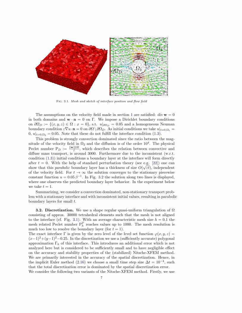
w in term of field-lines is given in Fig. 3.1.

6

Ω1

Γ∂ΩD

Ω2

Fig. 3.1. Mesh and sketch of interface position and flow field

The assumptions on the velocity field made in section 1 are satisfied: div w = 0in both domains and w · n = 0 on Γ. We impose a Dirichlet boundary conditionson ∂ΩD := (x, y, z) ∈ Ω : x = 0, s.t. u|∂ΩD

= 0.05 and a homogeneous Neumanboundary condition ε∇u ·n = 0 on ∂Ω\∂ΩD. As initial conditions we take u|t=0,Ω1 =0, u|t=0,Ω2 = 0.05. Note that these do not fulfill the interface condition (1.3).

This problem is strongly convection dominated since the ratio between the mag-nitude of the velocity field in Ω2 and the diffusion is of the order 104. The physical

Peclet number PD := ‖w‖2Rε , which describes the relation between convective and

diffuse mass transport, is around 3000. Furthermore due to the inconsistent (w.r.t.condition (1.3)) initial conditions a boundary layer at the interface will form directlyafter t = 0. With the help of standard perturbation theory (see e.g. [22]) one canshow that this parabolic boundary layer has a thickness of size O(

√εt), independent

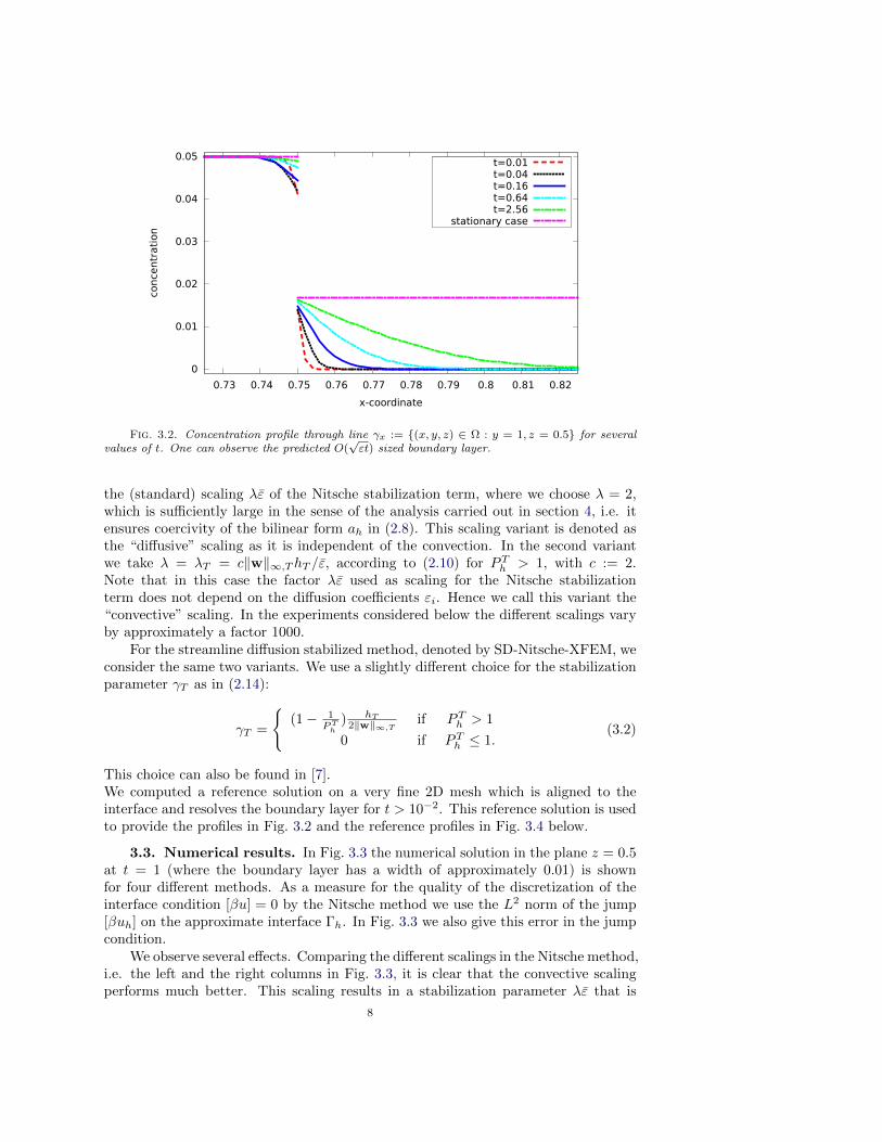
of the velocity field. For t → ∞ the solution converges to the stationary piecewiseconstant function u = 0.05β−1. In Fig. 3.2 the solution along two lines is displayed,where one observes the predicted boundary layer behavior. In the experiment belowwe take t = 1.

Summarizing, we consider a convection dominated, non-stationary transport prob-lem with a stationary interface and with inconsistent initial values, resulting in parabolicboundary layers for small t.

3.2. Discretization. We use a shape regular quasi-uniform triangulation of Ωconsisting of approx. 30000 tetrahedral elements such that the mesh is not alignedto the interface (cf. Fig. 3.1). With an average characteristic mesh size h = 0.1 themesh related Peclet number PTh reaches values up to 1000. The mesh resolution ismuch too low to resolve the boundary layer (for t = 1).The exact interface Γ is given by the zero level of the level set function ϕ(x, y, z) =(x−1)2+(y−1)2−0.25. In the discretization we use a (sufficiently accurate) polygonalapproximation Γh of this interface. This introduces an additional error which is notanalyzed here but is considered to be sufficiently small and to have negligible effecton the accuracy and stability properties of the (stabilized) Nitsche-XFEM method.We are primarily interested in the accuracy of the spatial discretization. Hence, inthe implicit Euler method (2.16) we choose a small time step size ∆t = 10−4, suchthat the total discretization error is dominated by the spatial discretization error.We consider the following two variants of the Nitsche-XFEM method. Firstly, we use

7

0

0.01

0.02

0.03

0.04

0.05

0.73 0.74 0.75 0.76 0.77 0.78 0.79 0.8 0.81 0.82

conce

ntr

ati

on

x-coordinate

t=0.01t=0.04t=0.16t=0.64t=2.56

stationary case

Fig. 3.2. Concentration profile through line γx := (x, y, z) ∈ Ω : y = 1, z = 0.5 for severalvalues of t. One can observe the predicted O(

√εt) sized boundary layer.

the (standard) scaling λε of the Nitsche stabilization term, where we choose λ = 2,which is sufficiently large in the sense of the analysis carried out in section 4, i.e. itensures coercivity of the bilinear form ah in (2.8). This scaling variant is denoted asthe “diffusive” scaling as it is independent of the convection. In the second variantwe take λ = λT = c‖w‖∞,ThT /ε, according to (2.10) for PTh > 1, with c := 2.Note that in this case the factor λε used as scaling for the Nitsche stabilizationterm does not depend on the diffusion coefficients εi. Hence we call this variant the“convective” scaling. In the experiments considered below the different scalings varyby approximately a factor 1000.

For the streamline diffusion stabilized method, denoted by SD-Nitsche-XFEM, weconsider the same two variants. We use a slightly different choice for the stabilizationparameter γT as in (2.14):

γT =

(1− 1

PTh

) hT

2‖w‖∞,Tif PTh > 1

0 if PTh ≤ 1.(3.2)

This choice can also be found in [7].We computed a reference solution on a very fine 2D mesh which is aligned to theinterface and resolves the boundary layer for t > 10−2. This reference solution is usedto provide the profiles in Fig. 3.2 and the reference profiles in Fig. 3.4 below.

3.3. Numerical results. In Fig. 3.3 the numerical solution in the plane z = 0.5at t = 1 (where the boundary layer has a width of approximately 0.01) is shownfor four different methods. As a measure for the quality of the discretization of theinterface condition [βu] = 0 by the Nitsche method we use the L2 norm of the jump[βuh] on the approximate interface Γh. In Fig. 3.3 we also give this error in the jumpcondition.

We observe several effects. Comparing the different scalings in the Nitsche method,i.e. the left and the right columns in Fig. 3.3, it is clear that the convective scalingperforms much better. This scaling results in a stabilization parameter λε that is

8

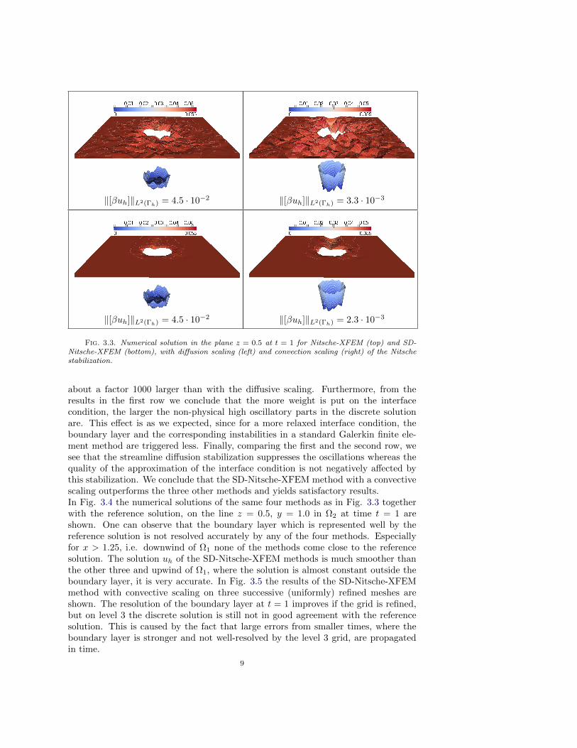
‖[βuh]‖L2(Γh) = 4.5 · 10−2 ‖[βuh]‖L2(Γh) = 3.3 · 10−3

‖[βuh]‖L2(Γh) = 4.5 · 10−2 ‖[βuh]‖L2(Γh) = 2.3 · 10−3

Fig. 3.3. Numerical solution in the plane z = 0.5 at t = 1 for Nitsche-XFEM (top) and SD-Nitsche-XFEM (bottom), with diffusion scaling (left) and convection scaling (right) of the Nitschestabilization.

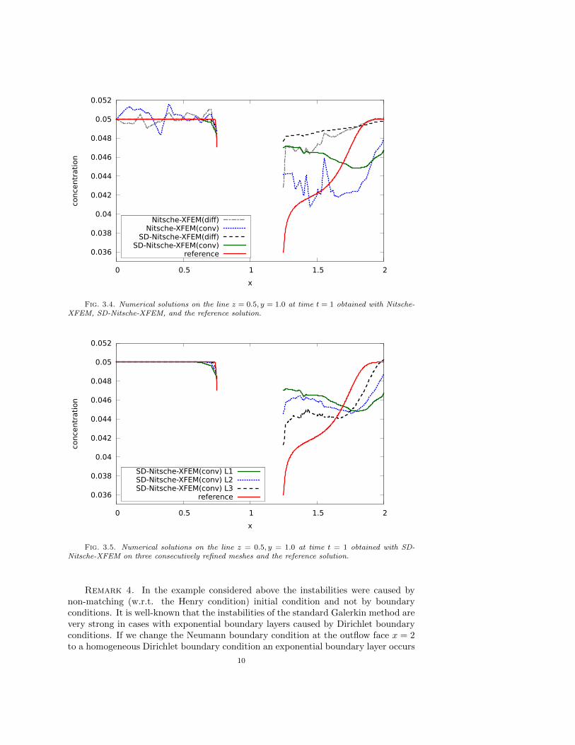
about a factor 1000 larger than with the diffusive scaling. Furthermore, from theresults in the first row we conclude that the more weight is put on the interfacecondition, the larger the non-physical high oscillatory parts in the discrete solutionare. This effect is as we expected, since for a more relaxed interface condition, theboundary layer and the corresponding instabilities in a standard Galerkin finite ele-ment method are triggered less. Finally, comparing the first and the second row, wesee that the streamline diffusion stabilization suppresses the oscillations whereas thequality of the approximation of the interface condition is not negatively affected bythis stabilization. We conclude that the SD-Nitsche-XFEM method with a convectivescaling outperforms the three other methods and yields satisfactory results.In Fig. 3.4 the numerical solutions of the same four methods as in Fig. 3.3 togetherwith the reference solution, on the line z = 0.5, y = 1.0 in Ω2 at time t = 1 areshown. One can observe that the boundary layer which is represented well by thereference solution is not resolved accurately by any of the four methods. Especiallyfor x > 1.25, i.e. downwind of Ω1 none of the methods come close to the referencesolution. The solution uh of the SD-Nitsche-XFEM methods is much smoother thanthe other three and upwind of Ω1, where the solution is almost constant outside theboundary layer, it is very accurate. In Fig. 3.5 the results of the SD-Nitsche-XFEMmethod with convective scaling on three successive (uniformly) refined meshes areshown. The resolution of the boundary layer at t = 1 improves if the grid is refined,but on level 3 the discrete solution is still not in good agreement with the referencesolution. This is caused by the fact that large errors from smaller times, where theboundary layer is stronger and not well-resolved by the level 3 grid, are propagatedin time.

9

0.036

0.038

0.04

0.042

0.044

0.046

0.048

0.05

0.052

0 0.5 1 1.5 2

conce

ntr

ati

on

x

Nitsche-XFEM(diff)Nitsche-XFEM(conv)

SD-Nitsche-XFEM(diff)SD-Nitsche-XFEM(conv)

reference

Fig. 3.4. Numerical solutions on the line z = 0.5, y = 1.0 at time t = 1 obtained with Nitsche-XFEM, SD-Nitsche-XFEM, and the reference solution.

0.036

0.038

0.04

0.042

0.044

0.046

0.048

0.05

0.052

0 0.5 1 1.5 2

conce

ntr

ati

on

x

SD-Nitsche-XFEM(conv) L1SD-Nitsche-XFEM(conv) L2SD-Nitsche-XFEM(conv) L3

reference

Fig. 3.5. Numerical solutions on the line z = 0.5, y = 1.0 at time t = 1 obtained with SD-Nitsche-XFEM on three consecutively refined meshes and the reference solution.

Remark 4. In the example considered above the instabilities were caused bynon-matching (w.r.t. the Henry condition) initial condition and not by boundaryconditions. It is well-known that the instabilities of the standard Galerkin method arevery strong in cases with exponential boundary layers caused by Dirichlet boundaryconditions. If we change the Neumann boundary condition at the outflow face x = 2to a homogeneous Dirichlet boundary condition an exponential boundary layer occurs

10

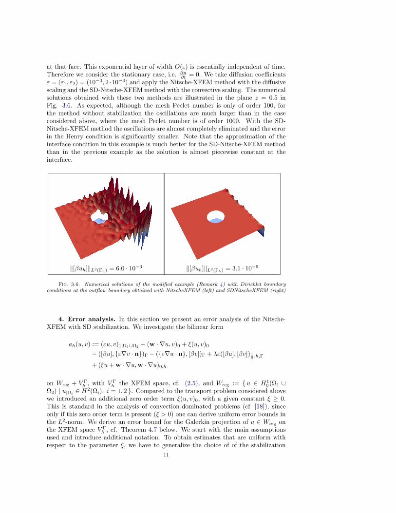
at that face. This exponential layer of width O(ε) is essentially independent of time.Therefore we consider the stationary case, i.e. ∂u

∂t = 0. We take diffusion coefficientsε = (ε1, ε2) = (10−3, 2 ·10−3) and apply the Nitsche-XFEM method with the diffusivescaling and the SD-Nitsche-XFEM method with the convective scaling. The numericalsolutions obtained with these two methods are illustrated in the plane z = 0.5 inFig. 3.6. As expected, although the mesh Peclet number is only of order 100, forthe method without stabilization the oscillations are much larger than in the caseconsidered above, where the mesh Peclet number is of order 1000. With the SD-Nitsche-XFEM method the oscillations are almost completely eliminated and the errorin the Henry condition is significantly smaller. Note that the approximation of theinterface condition in this example is much better for the SD-Nitsche-XFEM methodthan in the previous example as the solution is almost piecewise constant at theinterface.

‖[βuh]‖L2(Γh) = 6.0 · 10−3 ‖[βuh]‖L2(Γh) = 3.1 · 10−9

Fig. 3.6. Numerical solutions of the modified example (Remark 4) with Dirichlet boundaryconditions at the outflow boundary obtained with NitscheXFEM (left) and SDNitscheXFEM (right)

4. Error analysis. In this section we present an error analysis of the Nitsche-XFEM with SD stabilization. We investigate the bilinear form

ah(u, v) := (εu, v)1,Ω1∪Ω2 + (w · ∇u, v)0 + ξ(u, v)0

− ([βu], ε∇v · n)Γ − (ε∇u · n, [βv])Γ + λε([βu], [βv]) 12 ,h,Γ

+ (ξu+ w · ∇u,w · ∇u)0,h

on Wreg + V Γh , with V Γ

h the XFEM space, cf. (2.5), and Wreg := u ∈ H10 (Ω1 ∪

Ω2) | u|Ωi∈ H2(Ωi), i = 1, 2 . Compared to the transport problem considered above

we introduced an additional zero order term ξ(u, v)0, with a given constant ξ ≥ 0.This is standard in the analysis of convection-dominated problems (cf. [18]), sinceonly if this zero order term is present (ξ > 0) one can derive uniform error bounds inthe L2-norm. We derive an error bound for the Galerkin projection of u ∈ Wreg onthe XFEM space V Γ

h , cf. Theorem 4.7 below. We start with the main assumptionsused and introduce additional notation. To obtain estimates that are uniform withrespect to the parameter ξ, we have to generalize the choice of of the stabilization

11

parameter γT . If ξ = 0 we take γT as in (2.14). For the case ξ > 0 we take

γT :=

min

1ξ ,

2hT

‖w‖∞,T

if PTh > 1

min

1ξ ,

h2T

ε

if PTh ≤ 1.

(4.1)

This parameter choice is essentially the same as in [18]. The following estimates canbe derived:

γT ξ ≤ 1, γT ‖w‖∞,T ≤ 2hT , γ−1T h2

T ≤ ξh2T +

1

2‖w‖∞,ThT + ε. (4.2)

The family of triangulations Thh>0 is assumed to be shape regular, but not neces-sarily quasi-uniform. The triangulation Th is not assumed to be fitted to the interfaceΓ, but the resolution close to the interface should be sufficiently high such that theinterface can be resolved by the triangulation, in the sense that if Γ ∩ T =: ΓT 6= ∅then ΓT can be represented as the graph of a function on a planar cross-section ofT (cf. [10] for precise conditions). In the analysis of the Nitsche-XFEM method aninterpolation operator IΓ

h : Wreg → V Γh plays an important role. We recall the def-

inition of this operator. For i = 1, 2, let Ri be the restriction operator to Ωi, i.e.,(Riv)(x) = v(x) for x ∈ Ωi and (Riv)(x) = 0 otherwise. Let Ei : H2(Ωi)→ H2(Ω) bea bounded extension operator with Eiv = 0 on ∂Ω, and Ih : H2(Ω)∩H1

0 (Ω)→ Vh thestandard nodal interpolation operator corresponding to the space Vh of continuouslinear finite elements. The XFEM interpolation operator is given by

IΓh = R1IhE1R1 +R2IhE2R2.

Define Ti := T ∩ Ωi. Note that Ti can be very shape irregular. The constants thatoccur in the estimates in this section are independent of the shape regularity of Ti.For the interpolation operator IΓ

h optimal (local) interpolation error bounds can easilybe derived (cf. [10, 16]). The following holds:

‖u− IΓhu‖Hm(Ti) ≤ ‖EiRiu− IhEiRiu‖Hm(T )

≤ ch2−mT ‖EiRiu‖H2(T ), m = 0, 1, 2, for u ∈Wreg.

(4.3)

In the analysis below we use the assumptions div w = 0 on Ω, ‖w‖L∞(Ω) < ∞ andw · n = 0 on Γ.

We are particularly interested in the convection-dominated case, and thereforeallow ε = 1

2 (ε1 + ε2) ↓ 0, but we assume the ratio between ε1 and ε2 to be bounded,i.e. for i = 1, 2, we have ε/εi ≤ c with a uniform (for ε ↓ 0) constant c.

We assume that the constants βi used in the Henry condition are of order one.We will need several norms related to the Nitsche stabilization and the streamlinediffusion stabilization. The inner products (·, ·)0 and (·, ·)1,Ω1∪Ω2 (with correspondingnorms ‖·‖0 and |·|1,Ω1∪Ω2

) have been defined above in section 2. These inner productsdepend on a weighting with β, but this causes no problem since β is assumed to be oforder one. For the streamline diffusion stabilization we introduced the inner product(u, v)0,h =

∑T∈Th γT (u, v)0,T with corresponding norm denoted by ‖ · ‖0,h. In the

analysis of the Nitsche method the following norms are used:

‖v‖212 ,h,Γ

= (v, v) 12 ,h,Γ

=∑T∈T Γ

h

h−1T ‖v‖

2L2(ΓT ), ‖v‖

2− 1

2 ,h,Γ:=

∑T∈T Γ

h

hT ‖v‖2L2(ΓT ).

Recall that T Γh is the collection of T ∈ Th with ΓT = T ∩ Γ 6= ∅. We first derive

interpolation error bounds in different norms, which turn out to be useful.

12

The constants used in the results derived below are all independent of λ, ξ, ε, h, ‖w‖,and of how the interface Γ intersects the triangulation Th (i.e. of the shape regularityof Ti).

Lemma 4.1. For u ∈Wreg the following interpolation error bounds hold:

‖u− IΓhu‖0 ≤ ch2‖u‖2,Ω1∪Ω2

(4.4)

|u− IΓhu|1,Ω1∪Ω2

≤ ch‖u‖2,Ω1∪Ω2(4.5)√

ξ‖u− IΓhu‖0,h ≤ ch2‖u‖2,Ω1∪Ω2

(4.6)

‖w · ∇(u− IΓhu)‖0,h ≤ c‖w‖

12∞h

1 12 ‖u‖2,Ω1∪Ω2

(4.7)

2∑i=1

‖Ri(u− IΓhu)‖ 1

2 ,h,Γ≤ ch‖u‖2,Ω1∪Ω2 (4.8)

2∑i=1

‖n · ∇Ri(u− IΓhu)‖− 1

2 ,h,Γ≤ ch‖u‖2,Ω1∪Ω2 . (4.9)

Proof. The results in (4.4), (4.5) are known in the literature, e.g. [10, 16]. Forcompleteness we show how the result in (4.5) can be derived from (4.3):

|u− IΓhu|21,Ω1∪Ω2

=

2∑i=1

∑T∈Th

|u− IΓhu|21,Ti

≤ c2∑i=1

∑T∈Th

h2T ‖EiRiu‖22,T

≤ ch22∑i=1

‖EiRiu‖22,Ω ≤ ch22∑i=1

‖Riu‖22,Ωi= ch2‖u‖22,Ω1∪Ω2

.

The result in (4.4) can be proved using similar arguments. Using the choice of thestabilization parameter γT we obtain

ξ‖u− IΓhu‖20,h =

∑T∈Th

ξγT ‖u− IΓhu‖20,T ≤ ‖u− IΓ

hu‖20 ≤ ch4‖u‖22,Ω1∪Ω2,

and thus the result in (4.6) holds. The result in (4.7) follows from

‖w · ∇(u− IΓhu)‖20,h =

∑T∈Th

γT ‖w · ∇(u− IΓhu)‖20,T ≤

2∑i=1

∑T∈Th

γT ‖w‖2∞,T |u− IΓhu|21,Ti

≤ c‖w‖L∞(Ω)h|u− IΓhu|21,Ω1∪Ω2

≤ c‖w‖L∞(Ω)h3‖u‖22,Ω1∪Ω2

.

The results in (4.8), (4.9), are derived in [10]. The essential ingredient is the followingresult:

‖w‖2L2(ΓT ) ≤ c(h−1T ‖w‖

2L2(T ) + hT |w|21,T

)for all w ∈ H1(T ),

which holds for all T ∈ T Γh and with a constant c that is independent of the shape

13

regularity of Ti, cf. [10, 9]. For completeness we give a proof of (4.8):

2∑i=1

‖Ri(u− IΓhu)‖21

2 ,h,Γ=

2∑i=1

∑T∈T Γ

h

h−1T ‖EiRiu− IhEiRiu‖

2L2(ΓT )

≤ c2∑i=1

∑T∈T Γ

h

(h−2T ‖EiRiu− IhEiRiu‖

2L2(T ) + |EiRiu− IhEiRiu|21,T

)

≤ ch22∑i=1

∑T∈T Γ

h

‖EiRiu‖22,T ≤ ch22∑i=1

‖EiRiu‖22,Ω

≤ ch22∑i=1

‖Riu‖22,Ωi= ch2‖u‖22,Ω1∪Ω2

.

The result in (4.9) can be proved with similar arguments.

As we will see below, we can derive an ellipticity and continuity result for the bi-linear form ah(·, ·) with respect to a suitable norm. As expected this norm involvesterms that come from the Nitsche stabilization and from the streamline diffusionstabilization. To simplify the presentation we split the bilinear form in two parts(corresponding to Nitsche and streamline diffusion stabilization) and first considerthese two parts separately. Afterwards the results for these two parts can easily beglued together. We use the splitting

ah(u, v) = aNh (u, v) + aSDh (u, v)

aNh (u, v) =1

2(εu, v)1,Ω1∪Ω2

− ([βu], ε∇v · n)Γ − (ε∇u · n, [βv])Γ

+ λε([βu], [βv]) 12 ,h,Γ

aSDh (u, v) =1

2(εu, v)1,Ω1∪Ω2

+ (w · ∇u, v)0 + ξ(u, v)0 + (ξu+ w · ∇u,w · ∇u)0,h.

Corresponding norms are defined as

‖v‖2N =1

2ε|v|21,Ω1∪Ω2

+ λε‖[βv]‖212 ,h,Γ

‖v‖2SD =1

2ε|v|21,Ω1∪Ω2

+ ξ‖v‖20 + ‖w · ∇v‖20,h.

Lemma 4.2. There exists a constant c > 0 such that

aSDh (vh, vh) ≥ c‖vh‖2SD for all vh ∈ V Γh .

Proof. We apply partial integration to the term (w · ∇vh, vh)0. Since vh may bediscontinuous across Γ we have to split the integral. Using w · n = 0, div w = 0 andvh(x) = 0 for x ∈ ∂Ω we obtain

(w · ∇vh, vh)0 =

2∑i=1

∫Ωi

βiw · ∇vh vh dx =

2∑i=1

∫∂Ωi∩∂Ω

βiv2h w · nΩ ds

+

∫Γ

[βv2h]w · n ds−

2∑i=1

∫Ωi

βiw · ∇vh vh + βi(div w)v2h dx

= −(w · ∇vh, vh)0.

(4.10)

14

Hence, (w · ∇vh, vh)0 = 0 holds. Furthermore, using γT ξ ≤ 1 we get

ξ(vh,w · ∇vh)0,h = ξ∑T∈Th

γT (vh,w · ∇vh)0,T

≤ 1

2

∑T∈Th

ξ2γT ‖vh‖20,T + γT ‖w · ∇vh‖20,T

≤ 1

2ξ‖vh‖20 +

1

2‖w · ∇vh‖20,h.

Hence,

aSDh (vh, vh) ≥ 1

2minε1, ε2‖vh‖21,Ω1∪Ω2

+ ξ‖vh‖20 + ‖w · ∇vh‖20,h + ξ(vh,w · ∇vh)0,h

≥ cε‖vh‖21,Ω1∪Ω2+

1

2ξ‖vh‖20 +

1

2‖w · ∇vh‖20,h,

with a constant c > 0 which depends only on the ratio between ε1 and ε2, which isassumed to be bounded.

Lemma 4.3. There exists a constant c such that

aSDh (u−IΓhu, vh) ≤ c

(√ε+√‖w‖∞h+

√ξ h)h‖u‖2,Ω1∪Ω2

‖vh‖SD ∀ u ∈Wreg, vh ∈ V Γh .

Proof. We use the notation eh := u− IΓhu and recall the definition of aSDh (·, ·):

aSDh (eh, vh) =1

2(εeh, vh)1,Ω1∪Ω2

+(w·∇eh, vh)0+ξ(eh, vh)0+(ξeh+w·∇eh,w·∇vh)0,h.

Using the interpolation error bounds of lemma 4.1 we obtain

1

2(εeh, vh)1,Ω1∪Ω2

≤ c√ε h‖u‖2,Ω1∪Ω2

‖vh‖SD

ξ(eh, vh)0 ≤ c√ξh2‖u‖2,Ω1∪Ω2‖vh‖SD

ξ(eh,w · ∇vh)0,h ≤ c√ξh2‖u‖2,Ω1∪Ω2

‖vh‖SD

(w · ∇eh,w · ∇vh)0,h ≤ c‖w‖12∞h

1 12 ‖u‖2,Ω1∪Ω2

‖vh‖SD.

To the term (w · ∇eh, vh)0 we apply partial integration as in (4.10), resulting in

(w · ∇eh, vh)0 = −(eh,w · ∇vh)0 ≤( ∑T∈Th

γ−1T ‖eh‖

20,T

) 12 ‖vh‖SD

≤ c(ξh2 + ‖w‖∞h+ ε)

12h‖u‖2,Ω1∪Ω2

‖vh‖SD,

where in the last inequality we used the bound for γ−1T h2

T given in (4.2). Combiningthese estimates completes the proof.

We now turn to the analysis of the Nitsche bilinear form aNh (·, ·). We need the followinginverse inequality given in [10]. For completeness we include its elementary proof.

Lemma 4.4. There exists a constant cI independent of ε such that

‖ε∇vh · n‖− 12 ,h,Γ

≤ cI ε|vh|1,Ω1∪Ω2for all vh ∈ V Γ

h .

15

Proof. Let Pk be the space of polynomials of degree at most k. Using a scalingargument it follows that there exists a constant c, depending only on k and the shaperegularity of the triangulation Th, such that

hTκi‖p‖2L2(ΓT ) ≤ c‖p‖2L2(Ti)

for al p ∈ Pk, T ∈ T Γh , i = 1, 2. (4.11)

Using this we get

‖ε∇vh · n‖2− 12 ,h,Γ

≤ 2

2∑i=1

κ2i ‖εi∇(vh)i · n‖2− 1

2 ,h,Γ

= 2

2∑i=1

∑T∈T Γ

h

hTκ2i ‖εi∇(vh)i · n‖2L2(ΓT ) ≤ cε

2∑i=1

∑T∈T Γ

h

|vh|21,Ti≤ cε|vh|21,Ω1∪Ω2

,

and thus the result holds.

We now derive an ellipticity result for aNh (·, ·):Lemma 4.5. There exist constants c1 > 0, cs > 0 such that for λ > cs

aNh (vh, vh) ≥ c1‖vh‖2N for all vh ∈ V Γh .

Proof. Define c = 12ε

minε1, ε2 ≤ 12 and take λ ≥ 4c2I c

−1 with cI from lemma 4.4.The following holds:

aNh (vh, vh) ≥ cε|vh|21,Ω1∪Ω2− 2‖[βvh]‖ 1

2 ,h,Γ‖ε∇vh · n‖− 1

2 ,h,Γ+ λε‖[βvh]‖21

2 ,h,Γ

≥ cε|vh|21,Ω1∪Ω2− 2cI ε‖[βvh]‖ 1

2 ,h,Γ|vh|1,Ω1∪Ω2

+ λε‖[βvh]‖212 ,h,Γ

≥ 1

2cε|vh|21,Ω1∪Ω2

+ (λ− 2c2I c−1)ε‖[βvh]‖21

2 ,h,Γ

≥ 1

2cε|vh|21,Ω1∪Ω2

+1

2λε‖[βvh]‖21

2 ,h,Γ≥ c‖vh‖2N .

Lemma 4.6. There exists a constant c such that for λ > 0

aNh (u− IΓhu, vh) ≤ c

√ε(√λ+

1√λ

)h‖u‖2,Ω1∪Ω2

‖vh‖N

holds for all u ∈Wreg, vh ∈ V Γh .

Proof. We use the notation eh := u− IΓhu and recall the definition of aNh (·, ·):

aNh (eh, vh) =1

2(εeh, vh)1,Ω1∪Ω2

− ([βeh], ε∇vh · n)Γ − (ε∇eh · n, [βvh])Γ

+ λε([βeh], [βvh]) 12 ,h,Γ

.

Using the interpolation error bounds of lemma 4.1 and the inverse inequality in

16

lemma 4.4 we obtain

1

2(εeh, vh)1,Ω1∪Ω2

≤ c√ε h‖u‖2,Ω1∪Ω2

‖vh‖N

−([βeh], ε∇vh · n)Γ ≤ ‖[βeh]‖ 12 ,h,Γ‖ε∇vh · n‖− 1

2 ,h,Γ

≤ cε2∑i=1

‖Rieh‖ 12 ,h,Γ|vh|1,Ω1∪Ω2

≤ c√ε h‖u‖2,Ω1∪Ω2

‖vh‖N

−(ε∇eh · n, [βvh])Γ ≤ ‖ε∇eh · n‖− 12 ,h,Γ‖[βvh]‖ 1

2 ,h,Γ

≤ cε2∑i=1

‖n · ∇Rieh‖− 12 ,h,Γ‖[βvh]‖ 1

2 ,h,Γ

≤ c√ε

λh‖u‖2,Ω1∪Ω2‖vh‖N

λε([βeh], [βvh]) 12 ,h,Γ

≤ λε‖[βeh]‖ 12 ,h,Γ‖[βvh]‖ 1

2 ,h,Γ≤ c√ελ h‖u‖2,Ω1∪Ω2‖vh‖N .

Combination of these estimates and using 1√λ

+√λ > 1 proves the result.

We now combine the estimates derived above for aNh (·, ·) and aSDh (·, ·). For this weintroduce the norm

|||v|||2 = ‖v‖2N + ‖v‖2SD = ε|v|21,Ω1∪Ω2+ ξ‖v‖20 + ‖w · ∇v‖20,h + λε‖[βv]‖21

2 ,h,Γ.

Note that the two terms ‖w ·∇v‖20,h and λε‖[βv]‖212 ,h,Γ

originate from the stabilization

terms in the streamline diffusion and the Nitsche method, respectively.We discuss the choice of the stabilization parameter λ in the Nitsche method.

For the error analysis in the norm ||| · ||| it is natural to balance the upper boundsin lemma 4.3 and in lemma 4.6. For simplicity we make the (weak) assumption thatξh2 ≤ c(ε+‖w‖∞h) holds, i.e. in the bound in lemma 4.3 the factor

√ε+√‖w‖∞h+√

ξ h can be replaced by√ε +

√‖w‖∞h. The factor

√ε(√λ + 1/

√λ) in the upper

bound in lemma 4.6 should balance the latter factor, i.e.,

√ε+

√‖w‖∞h ≈

√ε(√λ+ 1/

√λ).

This leads to the choice as in (2.9), namely λ = c‖w‖∞h/ε if ‖w‖∞h ≥ ε and λ = cotherwise. We take c = cs, cf. lemma 4.5, to guarantee ellipticity. A slightly refinederror analysis leads to a localized variant of this parameter choice given in remark 2.In the remainder we take λ as in (2.9), with c = cs, cf. lemma 4.5. To simplify thepresentation, in the estimates below the terms ‖w‖∞ are absorbed in the constant c.

From the interpolation error bounds in lemma 4.1, and using λε ≤ c(ε+‖w‖∞h) ≤c(ε+ h), we obtain

|||u− IΓhu||| ≤ c

(√ε+√h+

√ξ h)h‖u‖2,Ω1∪Ω2 for all u ∈Wreg. (4.12)

Theorem 4.7. For u ∈ Wreg let RGu ∈ V Γh be the Galerkin projection for the

bilinear form ah(·, ·), i.e. ah(RGu, vh) = ah(u, vh) for all vh ∈ V Γh . The following

holds:

|||u−RGu||| ≤ c(√ε+√h+

√ξ h)h‖u‖2,Ω1∪Ω2

for all u ∈Wreg. (4.13)

17

The constant c is independent of ε, h, ξ and of how the interface Γ intersects thetriangulation Th.

Proof. The proof uses standard arguments. Define χh = RGu− IΓhu ∈ V Γ

h . Usingthe results in the lemmas above we obtain, with a suitable c > 0,

|||χh|||2 = ‖χh‖2N + ‖χh‖2SD ≤ c(aNh (χh, χh) + aSDh (χh, χh)

)= c ah(χh, χh) = c ah(u− IΓ

hu, χh) = c aNh (u− IΓhu, χh) + c aSDh (u− IΓ

hu, χh)

≤ c(√ε+√h+

√ξ h)h‖u‖2,Ω1∪Ω2

|||χh|||.

The result follows from a triangle inequality and the interpolation error bound in(4.12).

We comment on the bound derived in (4.13). For the diffusion dominated case, i.e.ε ∼ 1, this result reduces to results known in the literature. We discuss the convectiondominated case ε ≤ h with ξ ∈ [0, 1] and write eh := u − RGu. Furthermore weassume h ≤ chT (quasi-uniformity of the family of triangulations). Using h ≤ cγT forall T ∈ Th we obtain from (4.13)

‖w · ∇eh‖L2(Ω) ≤ ch‖u‖2,Ω1∪Ω2.

Hence, as for the streamline diffusion finite element method with the standard linearfinite element space, we have an optimal error bound (uniformly in ε) for the derivativeof the error in streamline direction. Furthermore, from

λε‖[βeh]‖212 ,h,Γ

≤ ch3‖u‖22,Ω1∪Ω2,

and λε = ch, we obtain

‖[βeh]‖L2(Γ) ≤ ch1 12 ‖u‖2,Ω1∪Ω2

uniformly in ε. This bound of order h1 12 for the error in the jump approximation is

the same as for the diffusion dominated case. Finally, if we take ξ > 0 we obtain anL2-norm error bound that is the same as for the streamline diffusion finite elementmethod with the standard linear finite element space, namely

‖eh‖L2(Ω) ≤c√ξh1 1

2 ‖u‖2,Ω1∪Ω2.

Remark 5. As noted in Remark 3, the SD-Nitsche-XFEM method has a straight-forward extension to finite elements of higher order. We comment on the generaliza-tion of the error analysis presented above to the higher order case. The interpolationerror bounds in Lemma 4.1 can easily be generalized to higher order extended finiteelements. The result in Lemma 4.4, cf. (4.11), also holds for higher order elements,and using this the results for the Nitsche bilinear form in the Lemmas 4.5 and 4.6can be generalized. In the analysis of the streamline diffusion bilinear form, how-ever, a difficulty arises related to an inverse inequality needed in the analysis. Forhigher order finite elements the term (div(ε∇uh),w · ∇vh)0,h arises in the stream-line diffusion stabilization. In the analysis of the streamline diffusion method fora standard higher order finite element space Vh one uses an inverse inequality ofthe form ‖∆vh‖0,T ≤ µinvh

−1T |vh|1,T for all vh ∈ Vh, cf. [18]. Such a result does

not hold in a higher order XFEM space, since the supports Ti = T ∩ Ωi of the ad-ditional (discontinuous) basis functions can be very shape irregular. We only have

18

‖∆vh‖0,Ti≤ µ(Ti)h

−1Ti|vh|1,Ti

with a factor µ(Ti) that depends on the shape regularityof Ti. To control this, instead of (4.1), one can choose a stabilization parameter γTi

that is sufficiently small. This would yield a stability result as in Lemma 4.2. If, how-ever, this parameter is “too small” it is not likely that a result as in Lemma 4.3, whichuses the third inequality in (4.2), still holds. We did not investigate this further.

5. Note on mass conservation. We derive a mass conservation property ofthe stabilized semi-discretization in (2.15) for the case of a stationary interface, i.e.w ·n = 0. For this we replace the homogeneous Dirichlet boundary condition in (1.5)by a, in view of mass conservation, more natural one. Define the inflow boundary by∂Ω− := x ∈ ∂Ω | w · nΩ < 0 , where nΩ is the outward pointing unit normal on∂Ω, and ∂Ω+ := ∂Ω \ ∂Ω−. Instead of (1.5) we consider

(uw − ε∇u) · nΩ = uIw · nΩ on ∂Ω−, t ∈ [0, T ]

ε∇u · nΩ = 0 on ∂Ω+, t ∈ [0, T ],(5.1)

with uI a given mass inflow function. In the weak formulation we have to changeaccordingly the function space V to V := v ∈ H1(Ω1 ∪ Ω2) | [βv]Γ = 0 , andthe weak formulation is as follows, cf. (2.4): Determine u ∈ W 1(0, T ; V ) such thatu(0) = u0 and for almost all t ∈ (0, T ):

(du

dt, v)0 + a(u, v)−

∫∂Ω−

βuvw · nΩ ds = (f, v)0−∫∂Ω−

βuIvw · nΩ ds for all v ∈ V.(5.2)

Using w · n = 0 on Γ and div w = 0 in Ωi we get

(w · ∇u, β−1)0 =

∫Ω

w · ∇u dx =

2∑i=1

(∫∂Ωi

uw · nΩids−

∫Ωi

udiv w dx

)=

∫∂Ω−

uw · nΩ ds+

∫∂Ω+

uw · nΩ ds.

(5.3)

Using this and taking the test function v = 1β ∈ V in (5.2) we obtain the global mass

conservation property

d

dt

∫Ω

u dx+

∫∂Ω−

uIw · nΩ ds+

∫∂Ω+

uw · nΩ ds =

∫Ω

f dx. (5.4)

This relation can also be derived directly from the strong formulation in (1.1), byintegrating the equations in (1.1) over Ω, and using the relations in (1.2), (5.1),(5.3). We show that an analogon of the conservation law (5.4) holds for the Nitsche-XFEM stabilized discretization. Due to the modification of the boundary conditionthe XFEM space we use is given by V Γ

h := v ∈ H1(Ω1∪Ω2) | v|Tiis linear for all T ∈

Th, i = 1, 2. and the discretization in (2.15) is modified as follows: determine uh(t) ∈V Γh such that uh(0) = u0 and

(duhdt

, vh)0 + (duhdt

,w · ∇vh)0,h + ah(uh, vh) + (w · ∇uh,w · ∇vh)0,h

−∫∂Ω−

βuhvhw · nΩ ds = (f, vh)0 + (f,w · ∇vh)0,h −∫∂Ω−

βuIvhw · nΩ ds(5.5)

for all vh ∈ V Γh . For the discrete conservation property it is essential that the XFEM

space contains piecewise smooth functions that are allowed to be discontinuous across

19

Γ. In particular the piecewise constant function β−1 is contained in V Γh . Taking this

test function vh in (5.5) all terms with ∇vh vanish and for the Nitsche bilinear form,cf. (2.8), we have ah(uh, β

−1) = (w · ∇uh, β−1)0. Thus we obtain

d

dt

∫Ω

uh dx+

∫Ω

w · ∇uh dx−∫∂Ω−

uhw · nΩ ds =

∫Ω

f dx−∫∂Ω−

uIw · nΩ ds.

Using partial integration for the term∫

Ωw · ∇uh dx, as in (5.3), results in

d

dt

∫Ω

uh dx+

∫∂Ω−

uIw · nΩ ds+

∫∂Ω+

uhw · nΩ ds =

∫Ω

f dx,

which is the discrete global mass conservation analogon of the one in (5.4). Finallywe briefly consider a mass conservation property in each subdomain Ωi. We assume∂Ω1 ∩ ∂Ω = ∅, hence, ∂Ω1 = Γ. From (1.1) we get

d

dt

∫Ω1

u dx−∫

Γ

ε∇u · n ds =

∫Ω1

f dx,

and using (1.2) this conservation property can be rewritten as

d

dt

∫Ω1

u dx−∫

Γ

ε∇u · n ds =

∫Ω1

f dx (5.6)

For the discretization we obtain (using a suitable test function vh):

d

dt

∫Ω1

uh dx−∫

Γ

ε∇uh · n ds−λε

h

∫Γ

[βuh] ds =

∫Ω1

f dx.

Hence there is a discrepancy between∫

Ω1u dx and

∫Ω1uh dx that is controlled by

‖ε∇eh ·n‖L2(Γ) and λεh ‖[βeh]‖L2(Γ), eh := u− uh. From the error analysis it folows

that both terms tend to zero for h ↓ 0, i.e., we have a consistency property.

Remark 6. In view of applications the case of a non-stationary interface Γ(t) ismuch more interesting than that of a stationary one. We comment on a generalizationof the method in (2.16) to the former case. For an evolving interface Γ(t), instead ofthe weak formulation in (2.4), one has to consider a space-time variational formulationto obtain a well-posed problem, cf. [9]. A discretization of the time derivative by meansof finite difference approximations (as done here for a stationary interface) does nolonger lead to a consistent discretization if the interface Γ(t) is moving in time. Adiscretization based on a space-time formulation using a suitable space-time extendedfinite element space should be used. For a convection dominated problem this canbe combined with a space-time streamline diffusion stabilization. The developmentand analysis of such a space-time SD-Nitsche-XFEM method is a topic of currentresearch.

Acknowledgement. The authors gratefully acknowledge funding by the Ger-man Science Foundation (DFG) within the Priority Program (SPP) 1506 “TransportProcesses at Fluidic Interfaces”.

REFERENCES

20

[1] R. Becker, E. Burman, and P. Hansbo, A Nitsche extended finite element method for in-compressible elasticity with discontinuous modulus of elasticity, Comput. Methods Appl.Mech. Engrg., 198 (2009), pp. 3352–3360.

[2] T. Belytschko, N. Moes, S. Usui, and C. Parimi, Arbitrary discontinuities in finite elements,Int. J. Num. Meth. Eng., 50 (2001), pp. 993–1013.

[3] D. Bothe, M. Koebe, K. Wielage, J. Pruss, and H.-J. Warnecke, Direct numerical simu-lation of mass transfer between rising gas bubbles and water, in Bubbly Flows: Analysis,Modelling and Calculation, M. Sommerfeld, ed., Heat and Mass Transfer, Springer, 2004.

[4] D. Bothe, M. Koebe, K. Wielage, and H.-J. Warnecke, VOF-simulations of mass transferfrom single bubbles and bubble chains rising in aqueous solutions, in Proceedings 2003ASME joint U.S.-European Fluids Eng. Conf., Honolulu, 2003, ASME. FEDSM2003-45155.

[5] A. Chernov and P. Hansbo, An hp-Nitsche’s method for interface problems with noncon-forming unstructured finite element meshes, Lect. Notes Comput. Sci. Eng., 76 (2011),pp. 153–161.

[6] J. Chessa and T. Belytschko, An extended finite element method for two-phase fluids, ASMEJournal of Applied Mechanics, 70 (2003), pp. 10–17.

[7] H. Elman, D. Silvester, and A. Wathen, Finite Elements and Fast Iterative Solvers, OxfordUniversity Press, Oxford, 2005.

[8] S. Groß, V. Reichelt, and A. Reusken, A finite element based level set method for two-phaseincompressible flows, Comp. Visual. Sci., 9 (2006), pp. 239–257.

[9] S. Groß and A. Reusken, Numerical Methods for Two-phase Incompressible Flows, Springer,Berlin, 2011.

[10] A. Hansbo and P. Hansbo, An unfitted finite element method, based on nitsche’s method, forelliptic interface problems, Comput. Methods Appl. Mech. Engrg., 191 (2002), pp. 5537–5552.

[11] , A finite element method for the simulation of strong and weak discontinuities in solidmechanics, Comput. Methods Appl. Mech. Engrg., 193 (2004), pp. 3523–3540.

[12] A. Hansbo, P. Hansbo, and M. Larson, A finite element method on composite grids basedon Nitsche’s method, Math. Model. Numer. Anal., 37 (2003), pp. 495–514.

[13] P. Hansbo, C. Lovadina, I. Perugia, and G. Sangalli, A Lagrange multiplier method for thefinite element solution of elliptic interface problems using non-matching meshes., Numer.Math., 100 (2005), pp. 91–115.

[14] M. Ishii, Thermo-Fluid Dynamic Theory of Two-Phase Flow, Eyrolles, Paris, 1975.[15] M. Muradoglu and G. Tryggvason, A front-tracking method for computation of interfacial

flows with soluble surfactant, J. Comput. Phys., 227 (2008), pp. 2238–2262.[16] A. Reusken, Analysis of an extended pressure finite element space for two-phase incompressible

flows, Comp. Visual. Sci., 11 (2008), pp. 293–305.[17] A. Reusken and T. Nguyen, Nitsche’s method for a transport problem in two-phase incom-

pressible flows, J. Fourier Anal. Appl., 15 (2009), pp. 663–683.[18] H.-G. Roos, M. Stynes, and L. Tobiska, Numerical Methods for Singularly Perturbed Dif-

ferential Equations — Convection-Diffusion and Flow Problems, vol. 24 of Springer Seriesin Computational Mathematics, Springer-Verlag, Berlin, second ed., 2008.

[19] S. Sadhal, P. Ayyaswamy, and J. Chung, Transport Phenomena with Droplets and Bubbles,Springer, New York, 1997.

[20] J. Slattery, Advanced Transport Phenomena, Cambridge Universtiy Press, Cambridge, 1999.[21] A.-K. Tornberg and B. Engquist, A finite element based level-set method for multiphase

flow applications, Comp. Vis. Sci., 3 (2000), pp. 93–101.[22] F. Verhulst, Methods and Applications of Singularly Perturbations — Boundary Layers and

Multiple Timescale Dynamics, vol. 50 of Texts in Applied Mathematics, Springer-Verlag,Berlin, first ed., 2000.

21