Embed Size (px)
Citation preview
Optimal preconditioners for Nitsche-XFEM
discretizations of interface problems
Christoph Lehrenfeld∗ and Arnold Reusken†
Preprint No. 406 August 2014
Key words: ellitic interface problem, extended finite element space,
XFEM, unfitted finite element method, Nitsche method,preconditioning, space decomposition
AMS Subject Classifications: 65N12, 65N30
Institut fur Geometrie und Praktische Mathematik
RWTH Aachen
Templergraben 55, D-52056 Aachen, (Germany)
∗Institut fur Geometrie und Praktische Mathematik, RWTH-Aachen University, D-52056 Aachen,Germany ([email protected]).
†Institut fur Geometrie und Praktische Mathematik, RWTH-Aachen University, D-52056 Aachen,Germany ([email protected]).
Optimal preconditioners for Nitsche-XFEMdiscretizations of interface problems
Christoph Lehrenfeld∗ Arnold Reusken†
August 13, 2014
In the past decade, a combination of unfitted finite elements (or XFEM)with the Nitsche method has become a popular discretization method forelliptic interface problems. This development started with the introductionand analysis of this Nitsche-XFEM technique in the paper [A. Hansbo, P.Hansbo, Comput. Methods Appl. Mech. Engrg. 191 (2002)]. In general, theresulting linear systems have very large condition numbers, which dependnot only on the mesh size h, but also on how the interface intersects themesh. This paper is concerned with the design and analysis of optimalpreconditioners for such linear systems. We propose an additive subspacepreconditioner which is optimal in the sense that the resulting conditionnumber is independent of the mesh size h and the interface position. Wefurther show that already the simple diagonal scaling of the stifness matrixresults in a condition number that is bounded by ch−2, with a constant c thatdoes not depend on the location of the interface. Both results are proven forthe two-dimensional case. Results of numerical experiments in two and threedimensions are presented, which illustrate the quality of the preconditioner.
AMS subject classifications. 65N12, 65N30
Key words. ellitic interface problem, extended finite element space, XFEM, unfittedfinite element method, Nitsche method, preconditioning, space decomposition
∗Institut fur Geometrie und Praktische Mathematik, RWTH-Aachen University, D-52056 Aachen,Germany ([email protected]).
†Institut fur Geometrie und Praktische Mathematik, RWTH-Aachen University, D-52056 Aachen,Germany ([email protected]).
1
1 Introduction
Let Ω ∈ R, d = 2, 3, be a polygonal domain that is subdivided in two connectedsubdomains Ωi, i = 1, 2. For simplicity we assume that Ω1 is strictly contained in Ω, i.e.,∂Ω1 ∩ ∂Ω = ∅. The interface between the two subdomains is denoted by Γ = ∂Ω1 ∩ ∂Ω2.We are interested in interface problems of the following type:
−div(α∇u) = f in Ωi, i = 1, 2, (1.1a)
[[α∇u · n]]Γ = 0 on Γ, (1.1b)
[[βu]]Γ = 0 on Γ, (1.1c)
u = 0 on ∂Ω. (1.1d)
Here n is the outward pointing unit normal on Γ = ∂Ω1, [[·]] the usual jump operatorand α = αi > 0, β = βi > 0 in Ωi are piecewise constant coefficients. In general one hasα1 6= α2. If β1 = β2 = 1, this is a standard interface problem that is often considered inthe literature [7, 5, 4, 20]. For β1 6= β2 this model is very similar to models used for masstransport in two-phase flow problems [2, 1, 16, 17, 11]. Without loss of generality weassume βi ≥ 1. The interface condition in (1.1c) is then usually called the Henry interfacecondition. Note that if β1 6= β2, the solution u is discontinuous across the interface. Ifβ1 = β2 and α1 6= α2 the first (normal) derivative of the solution is discontinuous acrossΓ. In the setting of two-phase flows one is typically interested in moving interfaces andinstead of (1.1) one uses a time-dependent mass transport model. In this paper, however,we restrict to the simpler stationary case.
In the past decade, a combination of unfitted finite elements (or XFEM) with theNitsche method has become a popular discretization method for this type of interfaceproblems. This development started with the introduction and analysis of this Nitsche-XFEM technique in the paper [7]. Since then this method has been extended in severaldirections, e.g., as a fictitious domain approach, for the discretization of interface problemsin computational mechanics, for the discretization of Stokes interface problems and forthe discretization of mass transport problems with moving interfaces, cf. [3, 8, 9, 13, 14,15, 10]. Almost all papers on this subject treat applications of the method or presentdiscretization error analyses. Efficient iterative solvers for the discrete problem is a topicthat has hardly been addressed so far. In general, solving the resulting discrete problemefficiently is a challenging task due to the well-known fact that the conditioning of thestiffness matrix is sensitive to the position of the interface relative to the mesh. If theinterface cuts elements in such a way that the ratio of the areas (volumes) on both sidesof the interface is very large, the stiffness matrix becomes (very) ill-conditioned.
Recently, for stabilized versions of the Nitsche-XFEM method condition number boundsof the form ch−2, with a constant c that is independent of how the interface Γ intersectsthe triangulation, have been derived [3, 10, 20]. In [10] an inconsistent stabilizationis used to guarantee LBB-stability for the pair of finite element spaces used for theStokes interface problem. This stabilization also improves the conditioning of the stiffnessmatrix, leading to a ch−2 condition number bound. In [20] a stabilized variant of theNitsche-XFEM for the problem (1.1) is considered. For this method an ch−2 condition
2
number bound is derived.In this paper we consider the original Nitsche-XFEM method from [7] for the discretiza-
tion of (1.1), without any stabilization. In [7] for this method optimal discretizationerror bounds are derived. We prove that after a simple diagonal scaling the conditionnumber is bounded by ch−2, with a constant c that is independent of how the interface Γintersects the triangulation. We prove that an optimal preconditioner, i.e. the conditionnumber of the preconditioned matrix is independent of h and of how the interface Γintersects the triangulation, can be constructed from approximate subspace corrections.If in the subspace spanned by the continuous piecewise linears one applies a standardmultigrid preconditioner and in the subspace spanned by the discontinuous finite elementfunctions that are added close to the interface (the xfem basis functions) one applies asimple Jacobi diagonal scaling, the resulting additive subspace preconditioner is optimal.The latter is the main result of this paper. The analysis uses the very general theory ofsubspace correction methods [18, 19]. Our analysis applies to the two-dimensional case(d = 2), but we expect that a very similar optimality result holds for d = 3. This claim issupported by results of numerical experiments that are presented.
The results derived in this paper also hold (with minor modifications) if in (1.1b),(1.1c) one has a nonhomogeneous right-hand side. In such a case one has to modify theright-hand side functional in the variational formulation, but the discrete linear operatorsthat describe the discretization remain the same.
The outline of this paper is as follows. In section 2 the Nitsche-XFEM method from[7] for the discretization of (1.1) is described. In section 3 we study the direct sumsplitting of the XFEM space into three subspaces, namely a subspace of continuouspiecewise linears, and two subspaces of xfem functions on both sides of the interface. InTheorem 3.3, which is the main result of this paper, we prove that this is a uniformlystable splitting. Following standard terminology (as in [18, 19]) we introduce an additivesubspace preconditioner in section 4. Based on the stable splitting property the qualityof the preconditioner (i.e., the condition number of the preconditioned matrix) can easilybe analyzed. In section 5 we present results of some numerical experiments, both ford = 2 and d = 3.
2 The Nitsche-XFEM discretization
In this section we describe the Nitsche-XFEM discretization, which can be found atseveral places in the literature [7, 4].
Let Thh>0 be a family of shape regular simplicial triangulations of Ω. A triangulationTh consists of simplices T , with hT := diam(T ) and h := maxhT | T ∈ Th. Thetriangulation is unfitted. We introduce some notation for cut elements, i.e. elementsT ∈ Th with Γ ∩ T 6= ∅. The subset of these cut elements is denoted by T Γ
h := T ∈Th | T ∩ Γ 6= ∅. To simplify the presentation and avoid technical details we assume thatfor all T ∈ T Γ
h the intersection ΓT := T ∩ Γ does not coincide with a subsimplex of T (aface, edge or vertex of T ). Hence, we assume that ΓT subdivides T into two subdomainsTi := T ∩ Ωi with measd(Ti) > 0. We further assume that there is at least one vertex of
3
T that is inside domain Ωi, i = 1, 2. In the analysis we assume that T Γh is quasi-uniform.
Let Vh ⊂ H10 (Ω) be the standard finite element space of continuous piecewise linears
corresponding to the triangulation Th with zero boundary values at ∂Ω. Let xj | j =1, . . . n, with n = dimVh, be the set of internal vertices in the triangulation. The indexset is denoted by J = 1, . . . , n. Let (φj)j∈J be the nodal basis functions in Vh, whereφj corresponds to the vertex with index j. Let JΓ := j ∈ J | |Γ∩supp(φj)| > 0 be theindex set of those basis functions the support of which is intersected by Γ. The Heavisidefunction HΓ has the values HΓ(x) = 0 for x ∈ Ω1, HΓ(x) = 1 for x ∈ Ω2. Using this,for j ∈ JΓ we define an enrichment function Φj(x) := |HΓ(x)−HΓ(xj)|. We introduceadditional, so-called xfem basis functions φΓ
j := φjΦj , j ∈ JΓ. Note that φΓj (xk) = 0 for
all j ∈ JΓ, k ∈ J . Furthermore, for j ∈ JΓ and xj ∈ Ω1, we have supp(φΓj ) ⊂ Ω2 and
for xj ∈ Ω2, we have supp(φΓj ) ⊂ Ω1. Related to this, the index set JΓ is partitioned
in JΓ,2 := j ∈ JΓ | xj ∈ Ω1 and JΓ,1 := JΓ \ JΓ,2 = j ∈ JΓ | xj ∈ Ω2. Hence, forj ∈ JΓ,i the xfem basis function φΓ
j has its support in Ωi, i = 1, 2. The XFEM space isdefined by
V Γh := Vh ⊕ V x
h,1 ⊕ V xh,2 = Vh ⊕ V x
h with V xh,i := spanφΓ
j | j ∈ JΓ,i , (2.1)
and V xh := V x
h,1 ⊕ V xh,2.
Remark 2.1. The XFEM space V Γh can also be characterized as follows: vh ∈ V Γ
h if andonly if there exist finite element functions v1, v2 ∈ Vh such that (vh)|Ωi
= (vi)|Ωi, i = 1, 2.
From this characterization one easily derives optimal approximation properties of theXFEM space for functions that are piecewise smooth, cf. [7, 12].
In the literature, e.g., [7, 4], discretization with the space V Γh is also called an unfitted
finite element method.An L2-stability property of the basis (φj)j∈J ∪ (φΓ
j )j∈JΓof V Γ
h is given in [12].For the discretization of the equation (1.1) in the XFEM space we first introduce some
notation for scalar products. The L2 scalar product is denoted by (u, v)0 :=∫
Ω uv dx.Furthermore we define
(u, v)1,Ω1,2 := (∇u,∇v)L2(Ω1) + (∇u,∇v)L2(Ω2), u, v ∈ H1(Ω1,2) := H1(Ω1 ∪ Ω2),
with the semi-norm denoted by |·|1,Ω1,2 = (·, ·)121,Ω1,2
and norm ‖·‖1,Ω1,2 := (‖·‖20+|·|21,Ω1,2)
12 .
On the interface we introduce the scalar product
(f, g)Γ :=
∫Γfg ds (2.2)
and the mesh-dependent weighted L2 scalar product
(f, g) 12,h,Γ := h−1
∫Γfg ds. (2.3)
4
The Nitsche-XFEM discretization of the interface problem (1.1) reads as follows:Find uh ∈ V Γ
h such that
(αβuh, vh)1,Ω1,2 − (α∇uh · n, [[βvh]])Γ − (α∇vh · n, [[βuh]])Γ
+ (λ[[βuh]], [[βvh]]) 12,h,Γ = (βf, vh)0 for all vh ∈ V Γ
h .(2.4)
Here we used the average w := κ1w1 + κ2w2 with an element-wise constant κi = |Ti||T | .
This weighting in the averaging is taken from the original paper [7]. The stabilizationparameter λ ≥ 0 should be taken sufficiently large, λ > cλ maxαii=1,2, with a suitableconstant cλ only depending on the shape regularity of T ∈ Th.
Discretization error analysis for this method is available in the literature. In [7] optimalorder discretization error bounds are derived for the case β1 = β2 = 1. The case β1 6= β2
is treated in [15].For the development and analysis of preconditioners for the discrete problem, without
loss of generality we can restrict to the case β1 = β2 = 1. This is due to the followingobservation. We note that (also if β1 6= β2) we have βvh ∈ V Γ
h iff vh ∈ V Γh . Thus, by
rescaling the test functions vh and with α := αβ−1 the problem (2.4) can be reformulatedas follows: Find uh = βuh ∈ V Γ
h such that
(αuh, vh)1,Ω1,2 − (α∇uh · n, [[vh]])Γ − (α∇vh · n, [[uh]])Γ
+ (λ[[uh]], [[vh]]) 12,h,Γ = (f, vh)0 for all vh ∈ V Γ
h .(2.5)
The stiffness matrices corresponding to (2.4) and (2.5) are related by a simple basistransformation. In the remainder of the paper we only consider the preconditioningof the stiffness matrix corresponding to (2.5). Via the simple basis transformation thesolution to (2.5) directly gives a solution to (2.4).
Remark 2.2. In certain situations it may be (e.g., due to implementational aspects)less convenient to transform the discrete problem (2.4) into (2.5). If one wants tokeep the original formulation, it is easy to provide an (optimal) preconditioner for it,given a preconditioner for the transformed problem (2.5). We briefly explain this. Let(ψj)1≤j≤m denote the basis for V Γ
h , and A, A the stiffness matrices w.r.t. this basis of theproblems (2.4) and (2.5), respectively. Let T be the matrix representation of the mappingvh → β−1vh, for vh ∈ V Γ
h , i.e., the i-th row of T contains the coefficients ti,k such thatβ−1ψi =
∑mk=1 ti,kψk. Then the relation A = TATT holds. Given a preconditioner C
for A, we define C := TT CT as preconditioner for A. Due to the equality of spectra,σ(CA) = σ(CA), the quality of C as a preconditioner for A is the same as the qualityof C as a preconditioner for A.
We introduce a compact notation for the symmetric bilinear form used in (2.5). Forconvenience we write α instead of α, and we assume a global constant value for λ:
ah(u, v) := (αu, v)1,Ω1,2 − (α∇u · n, [[v]])Γ − (α∇v · n, [[u]])Γ + λ([[u]], [[v]]) 12,h,Γ. (2.6)
5
This bilinear form is well-defined on V Γh × V Γ
h . For the analysis we introduce the bilinearform and corresponding norm defined by
|||u|||2h = |u|21,Ω1,2+ λ‖[[u]]‖21
2,h,Γ
, u ∈ V Γh . (2.7)
In [7] it is shown that, for λ sufficiently large, the norm corresponding to the Nitschebilinear form is uniformly equivalent to ||| · |||h:
ah(u, u) ∼ |||u|||2h for all u ∈ V Γh . (2.8)
Here and in the remainder we use the symbol ∼ to denote two-sided inequalities withconstants that are independent of h and of how the triangulation is intersected by theinterface Γ. The constants in these inequalities may depend on α and λ. We also use .to denote one-sided estimates that have the same uniformity property. In the remainderwe assume that λ > 0 is chosen such that (2.8) holds.
3 Stable subspace splitting
We will derive an optimal preconditioner for the bilinear form in (2.6) using the theoryof subspace correction methods. Two excellent overview papers on this topic are [18, 19].The theory of subspace correction methods as described in these overview papers is a verygeneral one, with applications to multigrid and to domain decomposition methods. Weapply it for a relatively very simple case with three disjoint spaces. We use the notationand some main results from [19]. It is convenient to adapt our notation to the one of theabstract setting in [19]. The three subspaces in (2.1) are denoted by W0 = Vh, Wi = V x
h,i,i = 1, 2. Thus we have the direct sum decomposition
S := V Γh =W0 ⊕W1 ⊕W2. (3.1)
Below u = u0 + u1 + u2 ∈ S always denotes a decompositon with ul ∈ Wl, l = 0, 1, 2. Forthe norm induced by the bilinear form ah(·, ·) we use the notation
‖u‖h := ah(u, u)12 , u ∈ S.
Recall that this norm is uniformly equivalent to ||| · |||h, cf. (2.8). In theorem 3.3 below weshow that the splitting in (3.1) is stable w.r.t. the norm ‖ · ‖h.
The result in the next theorem is the key point in our analysis. We show that thesplitting of S into W0 and the subspace spanned by the xfem basis functions W1 ⊕W2 isstable. For this we restrict to the two-dimensional case d = 2. We use a transformationof certain patches to a reference patch on [0, 1]2. We first describe this transformation.We construct a subdivision of T Γ
h into patches ωk as follows, cf. Figure 3.1. We firstdefine a subset E of all edges that are intersected by Γ. Consider an edge E1 which isintersected by Γ such that one vertex V1 is in Ω1 and the other, V ∗1 , is in Ω2. We definethis edge as the first element in E . Now fix one direction along the interface and going inthis direction along Γ we get an ordered list of all edges intersected by Γ. As last edge
6
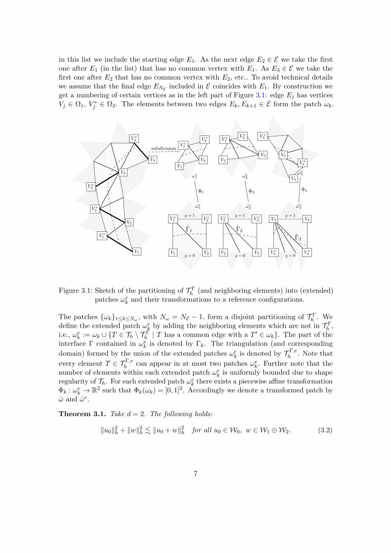
in this list we include the starting edge E1. As the next edge E2 ∈ E we take the firstone after E1 (in the list) that has no common vertex with E1. As E3 ∈ E we take thefirst one after E2 that has no common vertex with E2, etc.. To avoid technical detailswe assume that the final edge ENE included in E coincides with E1. By construction weget a numbering of certain vertices as in the left part of Figure 3.1: edge Ej has verticesVj ∈ Ω1, V ∗j ∈ Ω2. The elements between two edges Ek, Ek+1 ∈ E form the patch ωk.
V1
V2
V3
V4
V ∗1
V ∗2
V ∗3
V ∗4
subdivision
V1
V2
V ∗1
V ∗2
V1 V2
V ∗1 V ∗2
Γ1
y = 1
y = 0
ωe1
ωe1
Φ1
V2
V3
V ∗2V ∗3
V2 V3
V ∗2 V ∗3
Γ2
y = 1
y = 0
ωe2
ωe2
Φ2
V3
V4
V ∗3
V ∗4
V3 V4
V ∗3 V ∗4
Γ3
y = 1
y = 0
ωe3
ωe3
Φ3
Figure 3.1: Sketch of the partitioning of T Γh (and neighboring elements) into (extended)
patches ωek and their transformations to a reference configurations.
The patches ωk1≤k≤Nω , with Nω = NE − 1, form a disjoint partitioning of T Γh . We
define the extended patch ωek by adding the neighboring elements which are not in T Γh ,
i.e., ωek := ωk ∪ T ∈ Th \ T Γh | T has a common edge with a T ′ ∈ ωk. The part of the
interface Γ contained in ωek is denoted by Γk. The triangulation (and corresponding
domain) formed by the union of the extended patches ωek is denoted by T Γ,eh . Note that
every element T ∈ T Γ,eh can appear in at most two patches ωek. Further note that the
number of elements within each extended patch ωek is uniformly bounded due to shaperegularity of Th. For each extended patch ωek there exists a piecewise affine transformationΦk : ωek → R2 such that Φk(ωk) = [0, 1]2. Accordingly we denote a transformed patch byω and ωe.
Theorem 3.1. Take d = 2. The following holds:
‖u0‖2h + ‖w‖2h . ‖u0 + w‖2h for all u0 ∈ W0, w ∈ W1 ⊕W2. (3.2)
7
Proof. Due to norm equivalence the result in (3.2) is equivalent to:
|||u0|||2h + |||w|||2h . |||u0 + w|||2h for all u0 ∈ W0, w ∈ W1 ⊕W2.
For w ∈ W1 ⊕W2 we have w = 0 on Ω \ T Γ,eh , and T Γ,e
h is partitioned into patches ωek.Hence, it suffices to prove
|||u0|||2h,ωek
+ |||w|||2h,ωek. |||u0 + w|||2h,ωe
kfor all u0 ∈ W0, w ∈ W1 ⊕W2. (3.3)
We use the transformation to the reference patch ωe described above. On the referencepatch we have transformed spaces W0 (continuous, piecewise linears) and W1 ⊕ W2.The functions in W1 (W2) are piecewise linear on the part of the patch below (above)the interface Γ, zero on the line segment y = 0 (y = 1) and zero on the part ofthe patch above (below) the interface Γ. The norm |||u|||h,ωe
kand the induced norm
|||u|||ωek
=((∇u,∇u)L2(ωe
k) + λ([[u]], [[u]])L2(Γk)
) 12 , with u = u Φ−1
k on ωek, are uniformlyequivalent, because the constants in this norm equivalence are determined only by thecondition number of the piecewise affine transformation between ωek and ωek. Note that
neither the spaces Wl nor the norm ||| · |||ωek
depend on h (the h-dependence is implicitin the piecewise affine transformation). The reference patches ωek all have the samegeometric structure, cf. Figure 3.1. These patches have (due to shape regularity of Th) auniformly bounded number of vertices on the line segment that connects the vertices Vi,Vi+1 (or V ∗i , V ∗i+1). In the rest of the proof a generic reference patch and its extensionare denoted by ω and ωe, respectively. The interface segment that is intersected by ω isdenoted by Γ. We conclude that for (3.3) to hold it is sufficient to prove
|||u0|||2ωe + |||w|||2ωe ≤ K|||u0 + w|||2ωe for all u0 ∈ W0, w ∈ W1 ⊕ W2, (3.4)
with a constant K that is independent of how the patch ω is intersected by the interfaceΓ. Note that (∇u0,∇w)L2(ωe\ω) = ([[u0]], [[w]])L2(Γ) = 0 for u0 ∈ W0 and w ∈ W1 ⊕ W2.Hence,
|||u0 + w|||2ωe = |||u0|||2ωe + |||w|||2ωe + 2(∇u0,∇w)L2(ω), u0 ∈ W0, w ∈ W1 ⊕ W2
holds. Thus it suffices to prove the strengthened Cauchy-Schwarz inequality
(∇u0,∇w)L2(ω) ≤ C∗|||u0|||ωe |||w|||ωe for all u0 ∈ W0, w ∈ W1 ⊕ W2, (3.5)
with a uniform constant C∗ < 1. The proof of (3.5) is divided into three steps, namely astrengthened Cauchy-Schwarz inequality related to the x-derivative, a suitable Cauchy-Schwarz inequality related to the y-derivative and then combining these estimates.Step 1. The following holds:
|(ux, wx)L2(ω)| ≤ c0‖ux‖L2(ωe)‖wx‖L2(ω) for all u ∈W0, w ∈ W1 ⊕ W2, (3.6)
with a uniform constant c0 < 1. From the Cauchy-Schwarz inequality we get |(ux, wx)L2(ω)| ≤‖ux‖L2(ω)‖wx‖L2(ω). Within the patch ω = Ti the x-derivative ux is piecewise con-stant and ux|Ti = ux|Ti,N for the neighboring triangle Ti,N ∈ ωe \ ω. This implies
8
‖ux‖L2(Ti) ≤ c‖ux‖L2(Ti∪Ti,N ), with c < 1 depending only on shape regularity. Thus weobtain ‖ux‖L2(ω) ≤ c0‖ux‖L2(ωe), with a uniform constant c0 < 1, which yields (3.6).Step 2. The following holds:
|(uy, wy)L2(ω)| ≤ minc1‖ux‖L2(ω), ‖uy‖L2(ω)‖wy‖L2(ω)
+ c2‖uy‖L2(ω)‖[[w]]‖L2(Γ) for all u ∈W0, w ∈ W1 ⊕ W2,(3.7)
with suitable uniform constants c1, c2.Let Ti be the set of triangles that form ω and let these be ordered such that
meas1(Ti ∩ Ti+1) > 0. We denote the interior edges by ei = Ti ∩ Ti+1. To show (3.7) westart with partial integration∣∣∣ ∫
ωuywy dx
∣∣∣ =∣∣∣∑Ti
∫∂Ti
nTi,y uyw ds+
∫ΓTi
nΓ,y uy[[w]] ds∣∣∣
≤∑ei
∣∣∣[[uy]]ei∣∣∣∣∣∣ ∫ei
w ds∣∣∣+ ‖uy‖L2(Γ)‖[[w]]‖L2(Γ)
(3.8)
where for the edges of ∂Ti that lie on ∂ω = ∂[0, 1]2 we used w = 0 for y ∈ 0, 1 andnTi,y = 0 for x ∈ 0, 1. To proceed we need technical estimates to bound [[uy]]ei and∫eiw ds. For those estimates we exploit propertries of the geometry of ω. First consider
u ∈ W0 along an interior edge ei 6∈ ∂ω and denote the unit tangential vector to ei byτ = (τx, τy). For τ we have |τy| ≥ 1/
√2 ≥ |τx|. Due to continuity of u along ei there
holds [[∇u]]ei · τ = 0, which implies
|[[uy]]ei | =∣∣∣∣τxτy∣∣∣∣ |[[ux]]ei | ≤
∣∣ux|Ti∣∣+∣∣ux|Ti+1
∣∣.Thus we obtain
|[[uy]]ei | ≤ c min‖ux‖L2(Ti∪Ti+1), ‖uy‖L2(Ti∪Ti+1) . (3.9)
Next, we consider w = w1 + w2 ∈ W1 ⊕ W2 along the interior edge ei. Let Ti bea triangle adjacent to ei. Without loss of generality we assume that two vertices ofTi are in Ω1 and we thus have (w1)x = 0 on Ti. We denote the vertices of ei byxi = ei ∩ ∂ω ∩ Ωi, i = 1, 2 and the intersection point by xΓ = ei ∩ Γ and define thedistances di = ‖xi − xΓ‖2, i = 1, 2. As w is piecewise linear along ei, zero at x1, and(w1)x = 0 on Ti, we have w1(xΓ) = ±d1τy(w1)y. Furthermore:∫
ei
w ds =1
2d1w1(xΓ) +
1
2d2w2(xΓ) =
1
2(d1 + d2)w1(xΓ)− 1
2d2[[w]](xΓ).
We also have the geometrical information d1 ≤ d1 + d2 ≤√
2, d1 ≤ c|Ti|12 , |ΓTi | ≤
√2
and d2 ≤ c|ΓTi |12 . Because [[w]] is linear along ΓTi there also holds |ΓTi |
12 |[[w]](xΓ)| ≤
c‖[[w]]‖L2(ΓTi). Using these results we get∣∣∣ ∫
ei
w ds∣∣∣ ≤ c‖wy‖L2(Ti) + c‖[[w]]‖L2(ΓTi
). (3.10)
9
From (3.9) and (3.10) we obtain∑ei
∣∣∣[[uy]]ei∣∣∣∣∣∣ ∫ei
w ds∣∣∣ ≤ c‖uy‖L2(ω)‖[[w]]‖L2(Γ) + c‖ux‖L2(ω)‖wy‖L2(ω). (3.11)
Combining (3.8), (3.11) and the Cauchy-Schwarz inequality∣∣∣ ∫ω uywy dx∣∣∣ ≤ ‖uy‖L2(ω)‖wy‖L2(ω)
results in (3.7).Step 3. The following holds:
|(∇u,∇w)L2(ω)| ≤ C∗(‖ux‖L2(ωe) + ‖uy‖L2(ω)
) 12(‖∇w‖2L2(ω) + λ‖[[w]]‖2
L2(Γ)
) 12 (3.12)
for all u ∈W0, w ∈ W1 ⊕ W2, with a uniform constant C∗ < 1.The proof combines the preceding results. We define αx = ‖ux‖L2(ωe), βx = ‖wx‖L2(ω),
αy = ‖uy‖L2(ω), βy = ‖wy‖L2(ω), γ = ‖[[w]]‖L2(Γ). Then we have with (3.6), (3.7) and
θ = α2x
α2x+α2
y, α = (α2
x + α2y)
12 and β = (β2
x + β2y + λγ2)
12
|(∇u,∇w)L2(ω)| ≤ c0αxβx + minc1αx, αyβy + c2αyγ
≤ (c20α
2x + minc2
1α2x, α
2y+ c2
2α2yλ−1)
12 (β2
x + β2y + λγ2)
12
≤ (c20θ + minc2
1θ, 1− θ+ c22(1− θ)λ−1)
12αβ.
One easily sees that c20θ + minc2
1θ, 1 − θ ≤c20+c211+c21
< 1. For sufficiently large λ (λ >
1+c21c22(1−c20)
) (3.12) follows for a suitable uniform constant C∗ < 1.
The result (3.12) directly implies (3.5) and thus the estimate (3.2) holds for λ sufficientlylarge. For different values λ ≥ λ∗, with λ∗ the critical value for which the norm equivalence(2.8) holds, the norms ‖ · ‖h (depending on λ) are equivalent, with equivalence constantsdepending only on λ. This implies that (3.2) holds for any λ ≥ λ∗.
In the next lemma we derive the stable splitting property of W1 ⊕W2.
Lemma 3.2. The following holds:
‖ul‖h ∼ |ul|1,Ωlfor all ul ∈ Wl and l = 1, 2, (3.13)
‖u1‖2h + ‖u2‖2h . ‖u1 + u2‖2h for all u1 + u2 ∈ W1 ⊕W2. (3.14)
Proof. Take l = 1. We have
‖u1‖2h ∼ |||u1|||2h = |u1|21,Ω1+ λ‖[[u1]]‖21
2,h,Γ∼ |u1|21,Ω1
+ h−1‖u1‖2L2(Γ). (3.15)
This implies |u1|1,Ω1 . ‖u1‖h. Next we show
h−1‖u1‖2L2(Γ) . |u1|21,Ω1. (3.16)
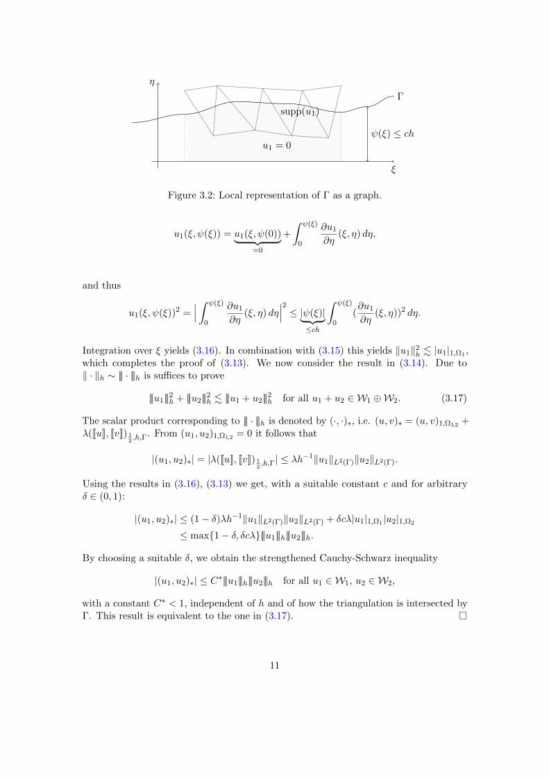
For this, we represent Γ locally as the graph of a function ψ, with a local coordinatesystem (ξ, η) as in Figure 3.2. Then we can write
10
ξ
η
ψ(ξ) ≤ ch
Γ
supp(u1)
u1 = 0
Figure 3.2: Local representation of Γ as a graph.
u1(ξ, ψ(ξ)) = u1(ξ, ψ(0))︸ ︷︷ ︸=0
+
∫ ψ(ξ)
0
∂u1
∂η(ξ, η) dη,
and thus
u1(ξ, ψ(ξ))2 =∣∣∣ ∫ ψ(ξ)
0
∂u1
∂η(ξ, η) dη
∣∣∣2 ≤ |ψ(ξ)|︸ ︷︷ ︸≤ch
∫ ψ(ξ)
0(∂u1
∂η(ξ, η))2 dη.
Integration over ξ yields (3.16). In combination with (3.15) this yields ‖u1‖2h . |u1|1,Ω1 ,which completes the proof of (3.13). We now consider the result in (3.14). Due to‖ · ‖h ∼ ||| · |||h is suffices to prove
|||u1|||2h + |||u2|||2h . |||u1 + u2|||2h for all u1 + u2 ∈ W1 ⊕W2. (3.17)
The scalar product corresponding to ||| · |||h is denoted by (·, ·)∗, i.e. (u, v)∗ = (u, v)1,Ω1,2 +λ([[u]], [[v]]) 1
2,h,Γ. From (u1, u2)1,Ω1,2 = 0 it follows that
|(u1, u2)∗| = |λ([[u]], [[v]]) 12,h,Γ| ≤ λh
−1‖u1‖L2(Γ)‖u2‖L2(Γ).
Using the results in (3.16), (3.13) we get, with a suitable constant c and for arbitraryδ ∈ (0, 1):
|(u1, u2)∗| ≤ (1− δ)λh−1‖u1‖L2(Γ)‖u2‖L2(Γ) + δcλ|u1|1,Ω1 |u2|1,Ω2
≤ max1− δ, δcλ|||u1|||h|||u2|||h.
By choosing a suitable δ, we obtain the strengthened Cauchy-Schwarz inequality
|(u1, u2)∗| ≤ C∗|||u1|||h|||u2|||h for all u1 ∈ W1, u2 ∈ W2,
with a constant C∗ < 1, independent of h and of how the triangulation is intersected byΓ. This result is equivalent to the one in (3.17).
11
As a direct consequence of the stable splitting properties derived above we obtain thefollowing main result.
Theorem 3.3. Take d = 2. There exists a constant K, independent of h and of how thetriangulation is intersected by Γ, such that
‖u0‖2h + ‖u1‖2h + ‖u2‖2h ≤ K‖u0 + u1 + u2‖2h for all u = u0 + u1 + u2 ∈ S.
Proof. Combine the result in (3.2) with the one in (3.14).
4 An optimal preconditioner based on approximate subspacecorrections
We describe and analyze an additive subspace decomposition preconditioner using theframework given in [19]. For this we first introduce some additional notation. LetQl : S → Wl, l = 0, 1, 2, be the L2-projection, i.e., for u ∈ S:
(Qlu,wl)0 = (u,wl)0 for all wl ∈ Wl.
The bilinear form ah(·, ·) on S that defines the discretization can be represented by theoperator A : S → S:
(Au, v)0 = ah(u, v) for all u, v ∈ S. (4.1)
The discrete problem (2.5) has the compact representation Au = fQ, where fQ is theL2-projection of the given data f ∈ L2(Ω) onto the finite element space S. The Ritzapproximations Al :Wl →Wl, l = 0, 1, 2, of A are given by
(Alu, v)0 = (Au, v) = ah(u, v) for all u, v ∈ Wl.
Note that these are symmetric positive definite operators. In the preconditioner we needsymmetric positive definite approximations Bl :Wl →Wl of the Ritz operators Al. Thespectral equivalence of Bl and Al is described by the following:
γl(Blu, u)0 ≤ (Alu, u)0 ≤ ρl(Blu, u)0 for all u ∈ Wl, (4.2)
with strictly positive constants γl, ρl, l = 0, 1, 2. The additive subspace preconditioner isdefined by
C =
2∑l=0
B−1l Ql. (4.3)
For the implementation of this preconditioner one has to solve (in parallel) three linearsystems. The operator Ql is not (explicitly) needed in the implementation, since if for agiven z ∈ S one has to determine dl = B−1
l Qlz, the solution can be obtained as follows:determine dl ∈ Wl such that
(Bldl, v)0 = (z, v)0 for all v ∈ Wl.
The theory presented in [19] can be used to quantify the quality of the preconditioner C.
12
Theorem 4.1. Define γmin = minl γl, ρmax = maxl ρl. Let K be the constant of thestable splitting in Theorem 3.3. The spectrum σ(CA) is real and
σ(CA) ⊂[γmin
K, 3ρmax
]holds.
Proof. We recall a main result from [19] (Theorem 8.1). If there are strictly positiveconstants K1,K2 such that
K−11
2∑l=0
(Blul, ul) ≤ ‖u0 + u1 + u2‖2h ≤ K2
2∑l=0
(Blul, ul) for all ul ∈ Wl
is satisfied, then σ(CA) ⊂ [K−11 ,K2] holds. For the lower inequality we use Theorem 3.3
and (4.2), which then results in
‖u0 + u1 + u2‖2h ≥ K−12∑l=0
‖ul‖2h = K−12∑l=0
(Alul, ul)0 ≥γmin
K
2∑l=0
(Blul, ul)0.
For the upper bound we note
‖u0 + u1 + u2‖2h ≤ 3
2∑l=0
‖ul‖2h = 3
2∑l=0
(Alul, ul)0 ≤ 3ρmax
2∑l=0
(Blul, ul)0.
Now we apply the above-mentioned result with K1 = K/γmin and K2 = 3ρmax.
The result in Theorem 3.3 yields that the constant K is independent of h and of howthe triangulation intersects the interface Γ. It remains to choose appropriate operatorsBl such that γmin and ρmax are uniform constants, too.
We first consider the approximation B0 of the Ritz-projection A0. Note that the finiteelement functions in W0 = Vh are continuous across Γ. This implies that
(A0u, v) = ah(u, v) = (αu, v)1,Ω1,2 = (α∇u,∇v)0 for all u, v ∈ W0.
Hence, A0 is a standard finite element discretization of a Poisson equation (with adiscontinuous diffusion coefficient α). As a preconditioner B0 for A0 we can use astandard symmetric multigrid method (which is a multiplicative subspace correctionmethod). From the literature [6, 18, 19] we know that for this choice of B0 we havespectral inequalities as in (4.2), with ρ0 = 1 and a constant γ0 > 0 that is independentof h and of how Γ intersects the triangulation.
It remains to find an appropriate preconditioner Bl of Al, l = 1, 2. For this wepropose the simple Jacobi method, i.e., diagonal scaling as a preconditioner for Al,l = 1, 2. We first introduce the operator Bl that represents the Jacobi preconditioner.Recall that Wl = spanφΓ
j | j ∈ JΓ,l. Elements u, v ∈ Wl have unique representations
13
u =∑
j∈JΓ,lαjφ
Γj , v =
∑j∈JΓ,l
βjφΓj . In terms of these representations the Jacobi
preconditioner is defined by
(Blu, v)0 =∑j∈JΓ,l
αjβjah(φΓj , φ
Γj ), u, v ∈ Wl, l = 1, 2. (4.4)
Note that ah(φΓj , φ
Γj ) are diagonal entries of the stiffness matrix corresponding to ah(·, ·).
The result in the next lemma shows that this diagonal scaling yields a robust preconditionerfor the Ritz operator Al.
Lemma 4.2. For the Jacobi preconditioner Bl there are strictly positive constants γl, ρl,independent of h and of how the triangulation is intersected by Γ such that
γl(Blu, u)0 ≤ (Alu, u)0 ≤ ρl(Blu, u)0 for all u ∈ Wl, l = 1, 2, (4.5)
holds.
Proof. Take u =∑
j∈JΓ,lαjφ
Γj ∈ Wl. For each T ∈ T Γ
h we define Tl = T ∩ Ωl, and for
each Tl we denote by V (Tl) the set vertices of T that are not in Ωl. Note that V (Tl) 6= ∅and V (Tl) does not contain all vertices of T . Using (3.13) and the construction of thexfem basis functions we get
(Blu, u)0 =∑j∈JΓ,l
α2jah(φΓ
j , φΓj ) ∼
∑j∈JΓ,l
α2j |φΓ
j |21,Ωl
=∑T∈T Γ
h
∑j∈V (Tl)
α2j |φΓ
j |21,Tl ∼∑T∈T Γ
h
∑j∈V (Tl)
α2j‖∇(φj)|T ‖22|Tl|.
(4.6)
Using (3.13) and the fact that ∇u is a constant vector on each Tl we get, with ‖ · ‖2 theEuclidean vector norm,
(Alu, u)0 = ‖u‖2h ∼ |u|21,Ωl=∑T∈T Γ
h
‖∇u‖2L2(Tl)=∑T∈T Γ
h
|Tl|‖(∇u)|Tl‖22. (4.7)
Now note that (∇u)|Tl =∑
j∈V (Tl)αj(∇φΓ
j )|Tl =∑
j∈V (Tl)αj∇(φj)|T . Because V (Tl)
does not contain all vertices of T , the vectors in the set (∇φj)|T | j ∈ V (Tl) areindependent and the angles between the vectors depend only on the geometry of thetriangulation Th. This implies that
‖(∇u)|Tl‖22 ∼
∑j∈V (Tl)
α2j‖∇(φj)|T ‖22.
Combining this with the results in (4.6) and (4.7) completes the proof.
Remark 4.1. Instead of an optimal multigrid preconditioner in the subspace W0 = Vh,one can also use a simpler (suboptimal) Jacobi preconditioner, i.e. B0 analogous to (4.4).For this choice the spectral constants in (4.2) are γ0 ∼ h2 and ρ0 ∼ 1. The three subspaces
14
are disjoint and thus if one applies a Jacobi preconditioner in the three subspaces, theadditive subspace preconditioner C in (4.3) coincides with a Jacobi preconditioner forthe operator A. From Theorem 4.1 we can conclude that κ(CA) ≤ ch−2 holds, with aconstant c independent on h and the cut position. Similar uniform O(h−2) conditionnumber bounds have recently been derived in the literature, cf. [20] and [4]. In thesepapers, however, for obtaining such a bound an additional stabilization term is added tothe bilinear form ah(·, ·). Our analysis shows that although the condition number of thestiffness matrix corresponding to ah(·, ·) does not have a uniform (w.r.t. the interfacecut) bound ch−2, a simple diagonal scaling results in a matrix with a spectral conditionnumber that is bounded by ch−2, with a constant c that is independent of how Γ isintersected by the triangulation. We note that adding a stabilization as treated [4] mayhave a positive effect not only on the condition number, but also on robustness of thediscretization w.r.t. large jumps in the diffusion coefficient.
Remark 4.2. The assumption d = 2 is essential only in the proof of Theorem 3.1.Concerning a generalization to d = 3 we note the following. Firstly, it is not obvious howthe subdivision into patches ωk can be generalized to three space dimensions. Secondly,if d = 2 then for every element within the reference patch ω we know that the localfinite element space on T ∩ Ωi is one-dimensional which is exploited to characterize theone-sided limit at the interface. In three dimensions the local finite element space canbe two-dimensional on both parts T ∩ Ωi, i = 1, 2 such that it is not obvious how togeneralize the proof of Theorem 3.1.
Nevertheless, we expect that the result of Theorem 3.3, hence also the results on theadditive subspace preconditioner, hold in three space dimensions. This claim is supportedby the results of a numerical example with d = 3, presented in section 5.2.
Remark 4.3. For ease of presentation, all dependencies on α, especially on the jumpsin α, have been absorbed in the constants that appear in the estimates. The results inneither Lemma 3.2, Theorem 3.1 nor Lemma 4.2 are robust with respect to jumps in α.We illustrate the dependence of the quality of the subspace preconditioner on the jumpsin α in a numerical example in section 5.1.
Remark 4.4. Instead of the additive preconditioner C in (4.3), one can also use amultiplicative version, cf. [19]. The optimality of this multiplicative variant, which canbe used as a solver or a preconditioner, can easily be derived using the framework givenin [19] and the results presented above.
5 Numerical experiments
In this section results for different subspace correction preconditioners are presented. Weconsider a discrete interface problem of the form: determine uh ∈ V Γ
h such that
ah(uh, vh) = (f, vh)0 for all vh ∈ V Γh ,
with ah(·, ·) as in(2.6). We take test problems with d = 2 and d = 3. The resultingstiffness matrix, which is the matrix representation of the operator A in (4.1), is denoted
15
by A. The matrices corresponding to the Ritz approximations A0 (projection on Vh) andAx (projection on V x
h ) are denoted by A0 and Ax, respectively. The diagonal matricesdiag(A), diag(A0) diag(Ax) are denoted by DA, D0 and Dx, respectively. Furthermore,C0 denotes a preconditioner for A0, for instance a multigrid preconditioner or C0 = D0.We define the block preconditioners
BA :=
(A0 00 Ax
), BD :=
(A0 00 Dx
), BC :=
(C0 00 Dx
). (5.1)
The matrix BA corresponds to an additive subspace preconditioner with exact subspacecorrections, BD has an exact correction in Vh and an approximate diagonal subspacecorrection in V x
h , and BC has approximate subspace corrections in all subspaces.In the following we study the performance of these preconditioners, in particular their
robustness w.r.t. both the variation in the mesh size h and the location of the interface.We also ilustrate the dependence of the condition numbers on λ and the diffusivityratio α1/α2. In section 5.1 we consider a two-dimensional example with a challengingconfiguration in the sense that many elements in the mesh have small cuts. This settingallows for a detailed study of the dependencies on h, α1/α2 and λ. In the second examplein section 5.2 we consider a three-dimensional analog and apply a multigrid preconditionerC0 for A0.
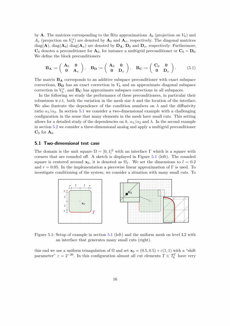
5.1 Two-dimensional test case
The domain is the unit square Ω = [0, 1]2 with an interface Γ which is a square withcorners that are rounded off. A sketch is displayed in Figure 5.1 (left). The roundedsquare is centered around x0, it is denoted as Ω1. We set the dimensions to l = 0.2and r = 0.05. In the implementation a piecewise linear approximation of Γ is used. Toinvestigate conditioning of the system, we consider a situation with many small cuts. To
Γ
l lr r
l
l
r
r
x0
x0
Figure 5.1: Setup of example in section 5.1 (left) and the uniform mesh on level L2 withan interface that generates many small cuts (right).
this end we use a uniform triangulation of Ω and set x0 = (0.5, 0.5) + ε(1, 1) with a “shiftparameter” ε = 2−20. In this configuration almost all cut elements T ∈ T Γ
h have very
16
small cuts (cf. right sketch in Figure 5.1). A similar test case has been considered in [3]as “sliver cut case”. We use four levels of uniform refinement denoted by L1,..,L4.
The diffusion parameters are fixed to (α1, α2) = (1.5, 2). Note that we considerβ1 = β2 = 1, but the problem is equivalent to every combination of Henry and diffusionparameters which fulfill (α1/β1, α2/β2) = (1.5, 2). The Nitsche stabilization parameter isset to λ = 4α with α = 1
2(α1 + α2) = 1.75. As a right-hand side source term we choosef = 1 in Ω1 and f = 0 in Ω2.
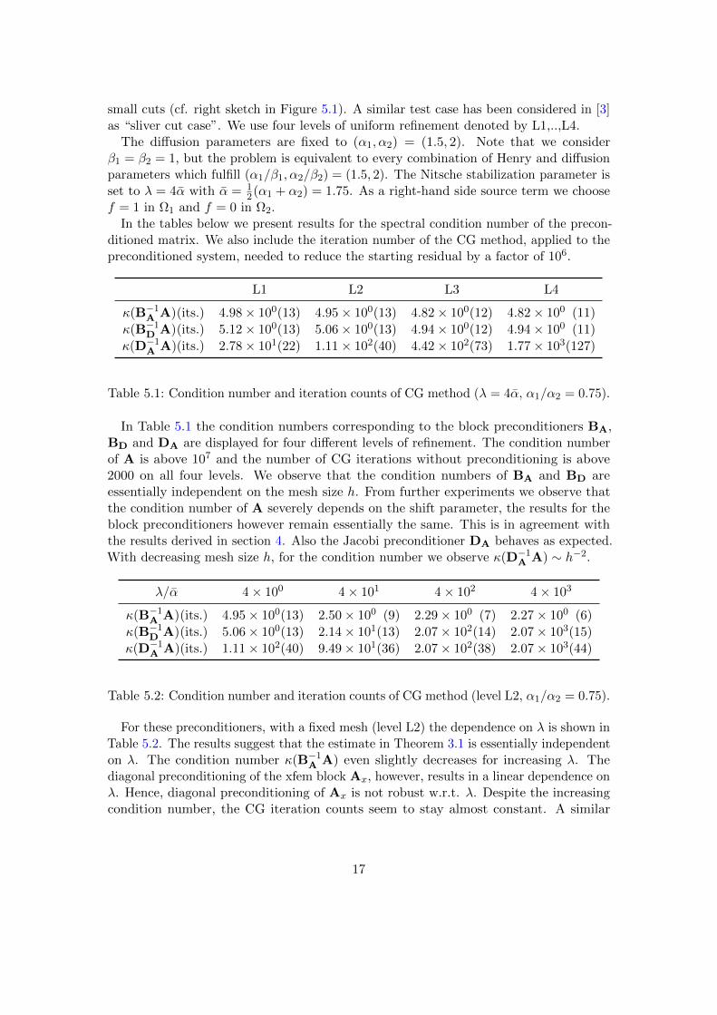
In the tables below we present results for the spectral condition number of the precon-ditioned matrix. We also include the iteration number of the CG method, applied to thepreconditioned system, needed to reduce the starting residual by a factor of 106.
L1 L2 L3 L4
κ(B−1A A)(its.) 4.98× 100(13) 4.95× 100(13) 4.82× 100(12) 4.82× 100 (11)
κ(B−1D A)(its.) 5.12× 100(13) 5.06× 100(13) 4.94× 100(12) 4.94× 100 (11)
κ(D−1A A)(its.) 2.78× 101(22) 1.11× 10²(40) 4.42× 10²(73) 1.77× 10³(127)
Table 5.1: Condition number and iteration counts of CG method (λ = 4α, α1/α2 = 0.75).
In Table 5.1 the condition numbers corresponding to the block preconditioners BA,BD and DA are displayed for four different levels of refinement. The condition numberof A is above 107 and the number of CG iterations without preconditioning is above2000 on all four levels. We observe that the condition numbers of BA and BD areessentially independent on the mesh size h. From further experiments we observe thatthe condition number of A severely depends on the shift parameter, the results for theblock preconditioners however remain essentially the same. This is in agreement withthe results derived in section 4. Also the Jacobi preconditioner DA behaves as expected.With decreasing mesh size h, for the condition number we observe κ(D−1
A A) ∼ h−2.
λ/α 4× 100 4× 101 4× 10² 4× 10³
κ(B−1A A)(its.) 4.95× 100(13) 2.50× 100 (9) 2.29× 100 (7) 2.27× 100 (6)
κ(B−1D A)(its.) 5.06× 100(13) 2.14× 101(13) 2.07× 10²(14) 2.07× 10³(15)
κ(D−1A A)(its.) 1.11× 10²(40) 9.49× 101(36) 2.07× 10²(38) 2.07× 10³(44)
Table 5.2: Condition number and iteration counts of CG method (level L2, α1/α2 = 0.75).
For these preconditioners, with a fixed mesh (level L2) the dependence on λ is shown inTable 5.2. The results suggest that the estimate in Theorem 3.1 is essentially independenton λ. The condition number κ(B−1
A A) even slightly decreases for increasing λ. Thediagonal preconditioning of the xfem block Ax, however, results in a linear dependence onλ. Hence, diagonal preconditioning of Ax is not robust w.r.t. λ. Despite the increasingcondition number, the CG iteration counts seem to stay almost constant. A similar
17
behavior can be observed for the Jacobi preconditioner DA.
α1/α2 7.5× 10⁻¹ 7.5× 100 7.5× 101 7.5× 10²
κ(B−1A A)(its.) 4.95× 100(13) 1.13× 101(20) 5.54× 101(26) 5.21× 10²(28)
κ(B−1D A)(its.) 5.06× 100(13) 1.29× 101(20) 9.87× 101(28) 9.61× 10²(26)
κ(D−1A A)(its.) 1.11× 10²(40) 6.33× 10²(45) 5.90× 10³(50) 5.86× 10⁴(72)
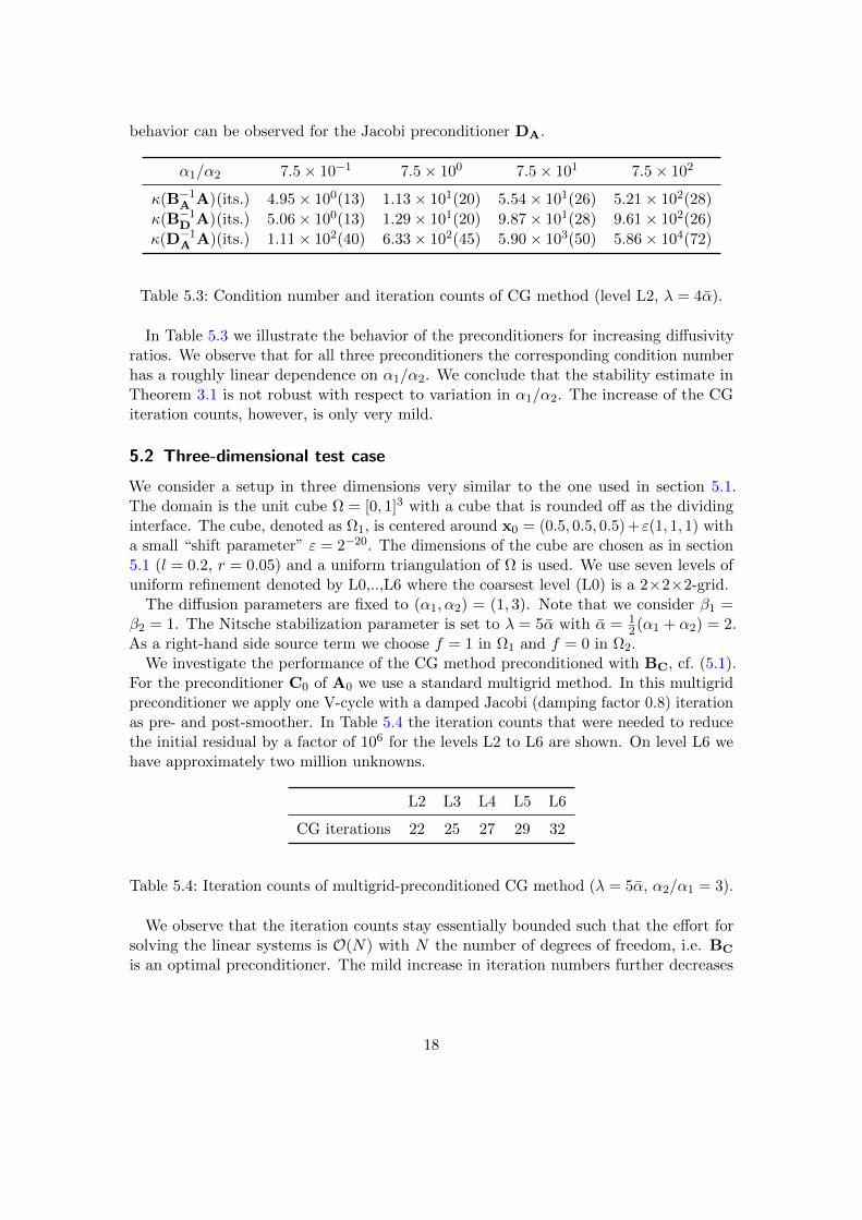
Table 5.3: Condition number and iteration counts of CG method (level L2, λ = 4α).
In Table 5.3 we illustrate the behavior of the preconditioners for increasing diffusivityratios. We observe that for all three preconditioners the corresponding condition numberhas a roughly linear dependence on α1/α2. We conclude that the stability estimate inTheorem 3.1 is not robust with respect to variation in α1/α2. The increase of the CGiteration counts, however, is only very mild.
5.2 Three-dimensional test case
We consider a setup in three dimensions very similar to the one used in section 5.1.The domain is the unit cube Ω = [0, 1]3 with a cube that is rounded off as the dividinginterface. The cube, denoted as Ω1, is centered around x0 = (0.5, 0.5, 0.5) + ε(1, 1, 1) witha small “shift parameter” ε = 2−20. The dimensions of the cube are chosen as in section5.1 (l = 0.2, r = 0.05) and a uniform triangulation of Ω is used. We use seven levels ofuniform refinement denoted by L0,..,L6 where the coarsest level (L0) is a 2×2×2-grid.
The diffusion parameters are fixed to (α1, α2) = (1, 3). Note that we consider β1 =β2 = 1. The Nitsche stabilization parameter is set to λ = 5α with α = 1
2(α1 + α2) = 2.As a right-hand side source term we choose f = 1 in Ω1 and f = 0 in Ω2.
We investigate the performance of the CG method preconditioned with BC, cf. (5.1).For the preconditioner C0 of A0 we use a standard multigrid method. In this multigridpreconditioner we apply one V-cycle with a damped Jacobi (damping factor 0.8) iterationas pre- and post-smoother. In Table 5.4 the iteration counts that were needed to reducethe initial residual by a factor of 106 for the levels L2 to L6 are shown. On level L6 wehave approximately two million unknowns.
L2 L3 L4 L5 L6
CG iterations 22 25 27 29 32
Table 5.4: Iteration counts of multigrid-preconditioned CG method (λ = 5α, α2/α1 = 3).
We observe that the iteration counts stay essentially bounded such that the effort forsolving the linear systems is O(N) with N the number of degrees of freedom, i.e. BC
is an optimal preconditioner. The mild increase in iteration numbers further decreases
18
if the Jacobi preconditioner Dx used in the subspace V xh is replaced by a symmetric
Gauss-Seidel preconditioner. For this choice we obtain the numbers 21,23,23,25,27 forthe levels L2 to L6.
Acknowledgement
The authors gratefully acknowledge funding by the German Science Foundation (DFG)within the Priority Program (SPP) 1506 “Transport Processes at Fluidic Interfaces”.
References
[1] D. Bothe, M. Koebe, K. Wielage, J. Pruss, and H.-J. Warnecke, Directnumerical simulation of mass transfer between rising gas bubbles and water, inBubbly Flows: Analysis, Modelling and Calculation, M. Sommerfeld, ed., Heat andMass Transfer, Springer, 2004.
[2] D. Bothe, M. Koebe, K. Wielage, and H.-J. Warnecke, VOF-simulations ofmass transfer from single bubbles and bubble chains rising in aqueous solutions, inProceedings 2003 ASME joint U.S.-European Fluids Eng. Conf., Honolulu, 2003,ASME. FEDSM2003-45155.
[3] E. Burman and P. Hansbo, Fictitious domain finite element methods using cutelements: II. A stabilized Nitsche method, Applied Numerical Mathematics, 62(2012), pp. 328 – 341. Third Chilean Workshop on Numerical Analysis of PartialDifferential Equations (WONAPDE 2010).
[4] E. Burman and P. Zunino, Numerical approximation of large contrast problemswith the unfitted Nitsche method, in Frontiers in Numerical Analysis - Durham 2010,J. Blowey and M. Jensen, eds., vol. 85 of Lecture Notes in Computational Scienceand Engineering, Springer Berlin Heidelberg, 2012, pp. 227–282.
[5] Z. Chen and J. Zhou, Finite element methods and their convergence for ellipticand parabolic interface problems, Numer. Math., 79 (1998), pp. 175–202.
[6] W. Hackbusch, Multi-Grid Methods and Applications, Springer-Verlag, Berlin,second ed., 2003.
[7] A. Hansbo and P. Hansbo, An unfitted finite element method, based on Nitsche’smethod, for elliptic interface problems, Comp. Methods Appl. Mech. Engrg., 191(2002), pp. 5537–5552.
[8] , A finite element method for the simulation of strong and weak discontinuitiesin solid mechanics, Comp. Methods Appl. Mech. Engrg., 193 (2004), pp. 3523–3540.
[9] P. Hansbo, Nitsche’s method for interface problems in computational mechanics,GAMM-Mitt., 28 (2005), pp. 183–206.
19
[10] P. Hansbo, M. G. Larson, and S. Zahedi, A cut finite element method for aStokes interface problem, Applied Numerical Mathematics, 85 (2014), pp. 90–114.
[11] M. Ishii, Thermo-Fluid Dynamic Theory of Two-Phase Flow, Eyrolles, Paris, 1975.
[12] A. Reusken, Analysis of an extended pressure finite element space for two-phaseincompressible flows, Comput. Vis. Sci., 11 (2008), pp. 293–305.
[13] A. Reusken and C. Lehrenfeld, Nitsche-XFEM with streamline diffusion sta-bilization for a two-phase mass transport problem, SIAM J. Sci. Comp., 34 (2012),pp. 2740–2759.
[14] , Analysis of a Nitsche XFEM-DG discretization for a class of two-phase masstransport problems, SIAM J. Num. Anal., 51 (2013), pp. 958–983.
[15] A. Reusken and T. Nguyen, Nitsche’s method for a transport problem in two-phase incompressible flows, J. Fourier Anal. Appl., 15 (2009), pp. 663–683.
[16] S. Sadhal, P. Ayyaswamy, and J. Chung, Transport Phenomena with Dropletsand Bubbles, Springer, New York, 1997.
[17] J. Slattery, L. Sagis, and E.-S. Oh, Interfacial Transport Phenomena, Springer,New York, second ed., 2007.
[18] J. Xu, Iterative methods by space decomposition and subspace correction, SIAMReview, 34 (1992), pp. 581–613.
[19] H. Yserentant, Old and new convergence proofs of multigrid methods, ActaNumerica, (1993), pp. 285–326.
[20] S. Zahedi, E. Wadbro, G. Kreiss, and M. Berggren, A uniformly well-conditioned, unfitted Nitsche method for interface problems: Part I, BIT NumericalMathematics, 53 (2013), pp. 791–820.
20