Nitrogen Oxides: Impacts On Public Health and the

Environment

Office of Air and RadiationUnited States Environmental Protection Agency

August 1997

Acknowledgments

This report was prepared by a team within the United StatesEnvironmental Protection Agency’s (EPA) Office of Air andRadiation and was coordinated with EPA’s Office of Water. Theprincipal author of this report was Doug Grano, Office of AirQuality Planning and Standards (OAQPS), Air Quality Strategiesand Standards Division, Research Triangle Park NC 27711. Authorsof specific sections were:

Doris Price and Rona BirnbaumOffice of Atmospheric Programs Acid Rain Division, EPA401 M Street S.W.Washington D.C. 20460Acid Deposition section;

Richard Batiuk, Chesapeake Bay Program Office, EPA410 Severn Avenue, Suite 109Annapolis MD 21403

and Melissa McCullough, OAQPS, EPAResearch Triangle Park NC 27711Eutrophication section; and

Dr. Roy Smith,OAQPS, EPAResearch Triangle Park NC 27711Toxic Products section.

Additional contributors to this report were as follows: JohnAckermann (EPA, OAQPS); John Bachmann (EPA, OAQPS); Dr. M. RobinsChurch (EPA, National Health and Environmental Effects ResearchLab, Corvallis, OR); Stephen Clark (EPA, Office of Ground Waterand Drinking Water); Ted Creekmore (EPA, OAQPS); Robin Dunkins(EPA, OAQPS); Chybryll Edwards (EPA, OAQPS); Barry Gilbert (EPA,OAQPS); Margaret Kerchner (National Oceanic and AtmosphericAdministration, Chesapeake Bay Office); Arnold Kuzmack, (EPA,Office of Science and Technology); Chris Lindhjem (EPA, Office ofMobile Sources); Ned Meyer (EPA, OAQPS); Roberta Parry (EPA,Office of Policy Planning and Evaluation); Bruce Polkowsky (EPA,OAQPS); Dr. Doug Ryan (United States Forest Service) and EricSlaughter (EPA, Oceans and Coastal Protection Division, Office ofWetlands, Oceans, and Watersheds).

This document was reviewed by the following scientificexperts: Dr. Ellis Cowling (North Carolina State University), Dr.Rudolph Husar (Washington University at St. Louis, MO), Dr.

Harvey Jefferies (University of North Carolina, Chapel Hill), Dr.Hans Paerl (University of North Carolina, Chapel Hill), Dr.Richard Stolarski (National Aeronautics and SpaceAdministration), and Dr. Mark Utell (University of RochesterMedical Center, NY). Their constructive comments providedcritical assistance to improving the scientific perspective ofthe final report.

Finally, public comments were invited on the November 1996draft of the document; discussion of the document and invitationto comment were provided through the Ozone Transport AssessmentGroup’s Implementation Strategies and Issues Workgroup and at theDecember 5, 1996 Clean Air Act Advisory Committee meeting. Thefinal document includes consideration by the authors of thecomments received from the public. Comments were received from:Colorado State University, Desert Research Institute, HoustonLighting & Power, Pacific Enterprises, Southern Company, Henry L.Stadler, and United States Forest Service.

Copies of this report may be downloaded from the Office ofAir and Radiation Policy and Guidance website athttp://www.epa.gov/ttn. Questions regarding this report shouldbe directed to Doug Grano at (919) 541-3292.

Nitrogen Oxides:Impacts on Public Health and the Environment

Table of Contents

Page

Executive Summary 1

I. Introduction/Overview 8

II. Clean Air Act Programs Involving Decreasesin Nitrogen Oxides(NO )Emissionsx

A. Acid Deposition 15

B. Nitrogen Dioxide 31

C. Ozone 36

D. Particulate Matter 52

E. Visibility Protection 65

III. Additional Public Health and Environmental Impacts from NO Emissionsx

A. Drinking Water 75

B. Eutrophication 79

C. Global Warming 93

D. Stratospheric Ozone Depletion 100

E. Terrestrial Ecosystems 104

F. Toxic Products 109

IV. Interprogram Issues

A. Local and Regional NO Controls 112x

B. Timing of NO Emissions Reductions: x

Seasonal or Year-Round 120

C. Interface with Other Control Programs:Three Examples of Secondary Emissions,EPA’s Clean Air Power Initiative, and New Standards for Ozone and Particulate Matter 126

Appendices

A. Mobile Source Programs 134

B. Stationary Source Programs 140

C. Sources and Sinks of Atmospheric Nitrogen 146

D. Acronyms and Abbreviations 155

Figures and Tables

Page

Figure I-1 National Anthropogenic NO Emissions by x

Source Category for 1994 and 2000 10

Figure I-2 National Total NO Emissions by Source x

Category for 1990 11

Figure I-3 Trends in NO Emissions for the Period x

1940 to 1994 13

Figure II-1 Map of Counties Potentially Not Meeting the 8-Hour Ozone Standard 39

Figure II-2 Map of Areas Not Meeting the 1-Hour Ozone Standard 40

Figure II-3 Map of Areas Not Meeting the Particulate Matter (PM ) Standard 5410

Figure II-4 Yearly Average Absolute and Relative Concentrations for Sulfate and Nitrate 59

Figure III-1 Greenhouse Gas Emissions 94

Figure III-2 Nitrous Oxide Emission Sources 96

Figure C-1 Plants in 1990 with Greater Than 1,000 Tons Per Year of NO Emissions 147x

Figure C-2 Density Map of 1994 NO Emissions 148x

Figure C-3 Trends in On-Road NO Emissions, Vehicle x

Miles Traveled, Fuel Use, and Gasoline Price 150

Table II-1 Utility Boiler Types and Emission Limits 17

Table II-2 Constituents of Atmospheric Fine Particles Less Than 2.5 Microns and Their Major Sources 61

Table II-3 Constituents of Atmospheric Particles Greater Than 2.5 Microns and Their Major Sources 62

Table II-4 Annual Averages (March 1988-February 1991) of Reconstructed Light Extinction (Mm ) for -1

19 Regions of the IMPROVE Network 72

Table III-1 Estimated Reductions in Nitrogen Loadings to Chesapeake Bay and Water Quality Response Under Several Control Scenarios 89

Table III-2 Estimated global sources of Nitrous Oxide 97

Table IV-1 Seasonal Emissions of NO , 1985 through 1994 124x

Table C-1 1994 National NO Emissions by Source Category 149x

Table C-2 Total National Emissions of NO , 1940 throughx

1994 151

Table C-3 Estimated Global Emissions of NO Typical of the x

Last Decade 152

Table C-4 Estimated Global Emissions of NH 1533

1

Nitrogen Oxides:Impacts On Public Health and the Environment

Executive Summary

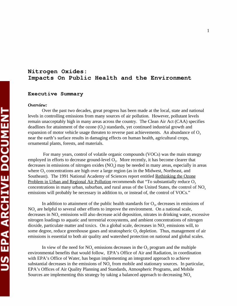
Overview:Over the past two decades, great progress has been made at the local, state and national

levels in controlling emissions from many sources of air pollution. However, pollutant levelsremain unacceptably high in many areas across the country. The Clean Air Act (CAA) specifiesdeadlines for attainment of the ozone (O ) standards, yet continued industrial growth and3

expansion of motor vehicle usage threaten to reverse past achievements. An abundance of O3

near the earth’s surface results in damaging effects on human health, agricultural crops,ornamental plants, forests, and materials.

For many years, control of volatile organic compounds (VOCs) was the main strategyemployed in efforts to decrease ground-level O . More recently, it has become clearer that3

decreases in emissions of nitrogen oxides (NO ) may be needed in many areas, especially in areasx

where O concentrations are high over a large region (as in the Midwest, Northeast, and3

Southeast). The 1991 National Academy of Sciences report entitled Rethinking the OzoneProblem in Urban and Regional Air Pollution recommends that “To substantially reduce O3

concentrations in many urban, suburban, and rural areas of the United States, the control of NOx

emissions will probably be necessary in addition to, or instead of, the control of VOCs.”

In addition to attainment of the public health standards for O , decreases in emissions of3

NO are helpful to several other efforts to improve the environment. On a national scale,x

decreases in NO emissions will also decrease acid deposition, nitrates in drinking water, excessivex

nitrogen loadings to aquatic and terrestrial ecosystems, and ambient concentrations of nitrogendioxide, particulate matter and toxics. On a global scale, decreases in NO emissions will, tox

some degree, reduce greenhouse gases and stratospheric O depletion. Thus, management of air3

emissions is essential to both air quality and watershed protection on national and global scales.

In view of the need for NO emissions decreases in the O program and the multiplex 3

environmental benefits that would follow, EPA’s Office of Air and Radiation, in coordinationwith EPA’s Office of Water, has begun implementing an integrated approach to achievesubstantial decreases in the emissions of NO from mobile and stationary sources. In particular,x

EPA’s Offices of Air Quality Planning and Standards, Atmospheric Programs, and MobileSources are implementing this strategy by taking a balanced approach to decreasing NOx

2

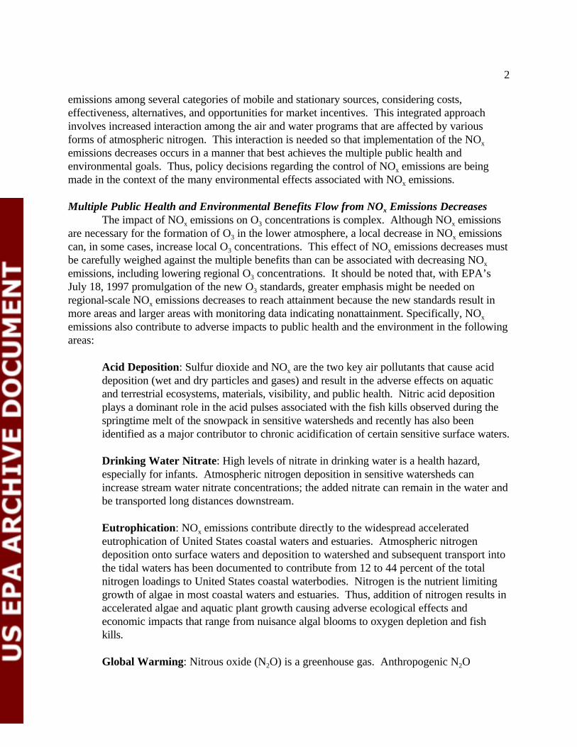
emissions among several categories of mobile and stationary sources, considering costs,effectiveness, alternatives, and opportunities for market incentives. This integrated approachinvolves increased interaction among the air and water programs that are affected by variousforms of atmospheric nitrogen. This interaction is needed so that implementation of the NOx

emissions decreases occurs in a manner that best achieves the multiple public health andenvironmental goals. Thus, policy decisions regarding the control of NO emissions are beingx

made in the context of the many environmental effects associated with NO emissions.x

Multiple Public Health and Environmental Benefits Flow from NO Emissions Decreasesx

The impact of NO emissions on O concentrations is complex. Although NO emissionsx 3 x

are necessary for the formation of O in the lower atmosphere, a local decrease in NO emissions3 x

can, in some cases, increase local O concentrations. This effect of NO emissions decreases must3 x

be carefully weighed against the multiple benefits than can be associated with decreasing NOx

emissions, including lowering regional O concentrations. It should be noted that, with EPA’s3

July 18, 1997 promulgation of the new O standards, greater emphasis might be needed on3

regional-scale NO emissions decreases to reach attainment because the new standards result inx

more areas and larger areas with monitoring data indicating nonattainment. Specifically, NOx

emissions also contribute to adverse impacts to public health and the environment in the followingareas:

Acid Deposition: Sulfur dioxide and NO are the two key air pollutants that cause acidx

deposition (wet and dry particles and gases) and result in the adverse effects on aquaticand terrestrial ecosystems, materials, visibility, and public health. Nitric acid depositionplays a dominant role in the acid pulses associated with the fish kills observed during thespringtime melt of the snowpack in sensitive watersheds and recently has also beenidentified as a major contributor to chronic acidification of certain sensitive surface waters.

Drinking Water Nitrate: High levels of nitrate in drinking water is a health hazard,especially for infants. Atmospheric nitrogen deposition in sensitive watersheds canincrease stream water nitrate concentrations; the added nitrate can remain in the water andbe transported long distances downstream.

Eutrophication: NO emissions contribute directly to the widespread acceleratedx

eutrophication of United States coastal waters and estuaries. Atmospheric nitrogendeposition onto surface waters and deposition to watershed and subsequent transport intothe tidal waters has been documented to contribute from 12 to 44 percent of the totalnitrogen loadings to United States coastal waterbodies. Nitrogen is the nutrient limitinggrowth of algae in most coastal waters and estuaries. Thus, addition of nitrogen results inaccelerated algae and aquatic plant growth causing adverse ecological effects andeconomic impacts that range from nuisance algal blooms to oxygen depletion and fishkills.

Global Warming: Nitrous oxide (N O) is a greenhouse gas. Anthropogenic N O2 2

3

emissions in the United States contribute about 2 percent of the greenhouse effect, relativeto total United States. anthropogenic emissions of greenhouse gases. In addition,emissions of NO lead to the formation of tropospheric O , which is another greenhousex 3

gas.

Nitrogen Dioxide (NO ): Exposure to NO is associated with a variety of acute and2 2

chronic health effects. The health effects of most concern at ambient or near-ambientconcentrations of NO include mild changes in airway responsiveness and pulmonary2

function in individuals with pre-existing respiratory illnesses and increases in respiratoryillnesses in children. Currently, all areas of the United States monitoring NO are below2

EPA’s threshold for health effects.

Nitrogen Saturation of Terrestrial Ecosystems: Nitrogen accumulates in watershedswith high atmospheric nitrogen deposition. Because most North American terrestrialecosystems are nitrogen limited, nitrogen deposition often has a fertilizing effect,accelerating plant growth. Although this effect is often considered beneficial, nitrogendeposition is causing important adverse changes in some terrestrial ecosystems, includingshifts in plant species composition and decreases in species diversity or undesirable nitrateleaching to surface and ground water and decreased plant growth.

Particulate Matter (PM): NO compounds react with other compounds in thex

atmosphere to form nitrate particles and acid aerosols. Because of their small size nitrateparticles have a relatively long atmospheric lifetime; these small particles can alsopenetrate deeply into the lungs. PM has a wide range of adverse health effects.

Stratospheric O Depletion: A layer of O located in the upper atmosphere (stratosphere)3 3

protects people, plants, and animals on the surface of the earth (troposphere) fromexcessive ultraviolet radiation. N O, which is very stable in the troposphere, slowly2

migrates to the stratosphere. In the stratosphere, solar radiation breaks it into nitric oxide(NO) and nitrogen (N). The NO reacts with O to form NO and molecular oxygen. 3 2

Thus, additional N O emissions would result in some decrease in stratospheric O .2 3

Toxic Products: Airborne particles derived from NO emissions react in the atmosphere x

to form various nitrogen containing compounds, some of which may be mutagenic. Examples of transformation products thought to contribute to increased mutagenicityinclude the nitrate radical, peroxyacetyl nitrates, nitroarenes, and nitrosamines.

Visibility and Regional Haze: NO emissions lead to the formation of compounds thatx

can interfere with the transmission of light, limiting visual range and color discrimination. Most visibility and regional haze problems can be traced to airborne particles in theatmosphere that include carbon compounds, nitrate and sulfate aerosols, and soil dust. The major cause of visibility impairment in the eastern United States is sulfates, while inthe West the other particle types play a greater role.

4

O Formation and Accumulation3

Although O formation and accumulation in the atmosphere involves complex nonlinear3

processes, a very simplified description of the process is offered here. In short, NO is formedduring high temperature combustion involving air (air being largely N and O ). The NO is2 2

converted to NO by reacting with either inorganic or organic radicals formed from oxidized2

VOCs or by reacting with O . The NO then photolyzes, leading to the formation of O and NO. 3 2 3

A reaction path that converts NO to NO without consuming a molecule of O allows O to2 3 3

accumulate; such a path is provided by inorganic and organic radicals that arise from VOCreactions.

The formation and accumulation of O is further complicated by the transport of O3 3

itself and O precursors (including NO ). This transport factor results in interactions between3 x

distant sources in urban or rural areas and local ambient O concentrations. The transport of O3 3

and precursor pollutants over hundreds of kilometers (or hundreds of miles) can be a significantfactor in the accumulation of O in certain areas. Another important complicating factor is the3

influence of meteorological factors on O formation, including temperature, wind direction, and3

wind speed.

In the 1990 amendments to the CAA, Congress recognized the importance of NOx

emissions reductions and, especially in the Northeast, the need for regional scale control programsto achieve the O standard. In section 184 of the CAA, Congress established the Northeast Ozone3

Transport Commission to address interstate transport of O pollution among 12 northeastern3

States and the District of Columbia. Further, Congress required large stationary sources locatedin the Northeast Ozone Transport region and in moderate, serious, severe and extreme O3

nonattainment areas throughout the country to decrease NO emissions.x

The extent of local controls that will be needed to attain and maintain the O national3

ambient air quality standards (NAAQS) in and near seriously polluted cities is sensitive both to theamount of O and O precursors transported into the local area and to the specific photochemistry3 3

of the area. In some cases, preliminary local modeling performed by the states for the 1-hour O3

standard indicates that it may not be feasible to find sufficient local control measures for individualnonattainment areas unless transport into the areas is significantly lowered. The EPA has alsoconducted preliminary analyses for the new 8-hour O standard which indicate that regional NO3 x

emissions decreases would be effective in helping many areas attain that standard. Thesemodeling studies suggest that decreasing NO emissions on a regional basis is effective inx

decreasing O over large geographic areas.3

NO Emissions Sources and Trendsx

Emissions of NO result from fuel combustion at high temperature, which occursx

principally in fossil fuel-fired electric utility and industrial boilers and in motor vehicle internalcombustion engines. Electric utility and motor vehicle emissions each represent about one-thirdof the total 1994 NO emissions. About 85 percent of the total NO emissions from electricx x

utilities are attributed to utilities burning coal.

5

From 1940 through 1970, annual NO emissions increased by a factor of three (fromx

7 million to 21 million tons). Since 1980, annual national NO emissions leveled off at about 23x

million tons. Data show that national NO emissions slightly increased from 1990-1993. In thex

mid-1990s, NO emissions are expected to decrease somewhat as stationary source NO controlsx x

and light-duty and heavy-duty tailpipe standards are implemented and enhanced vehicle inspectionand maintenance (I/M) programs begin in some O nonattainment areas. Electric utility NO3 x

emissions are expected to decline after 1999 as the phase II acid deposition standards becomeeffective. Despite increases in vehicle miles traveled, total on-road vehicle emissions will likelycontinue to decline through 2005 as per vehicle NO emissions decrease due to tighter tailpipex

standards, phase II reformulated gasoline is implemented, and I/M requirements are met. Soonafter the year 2002, overall NO emissions are projected to begin to increase and continue tox

increase in the foreseeable future due to increased economic activity.

General Conclusions and Implications for Future NO Management Strategiesx

It has become clearer that controls of NO emissions may be needed in many areas,x

especially in areas of the United States where O concentrations are high over a large region (as in3

the Midwest, Northeast, and Southeast). In addition to helping attain the NAAQS for O ,3

decreases in NO emissions will also likely help improve the environment by decreasing thex

adverse impacts of acid deposition, drinking water nitrate exposure, eutrophication ofwaterbodies, global warming, NO exposure, nitrogen saturation of terrestrial ecosystems, PM2

formation, stratospheric O depletion, toxics exposure, and visibility impairment. 3

Although total NO emissions will decline from current levels by the year 2000 because ofx

mandatory CAA programs, NO emissions will, soon after the year 2002, begin to graduallyx

increase. Both mobile, including non-road, and stationary sources are significant contributors tothe NO problem on a nationwide basis. Thus, new initiatives will be necessary to achievex

reductions in NO emissions that may be needed over much of the nation, especially to help attainx

the O standards. 3

The EPA has begun implementing an integrated approach to achieve reductions inemissions of NO . This integrated approach involves increased interaction among the air andx

water programs that are affected by various forms of atmospheric nitrogen and addresses severalcategories of mobile and stationary sources. Policy decisions regarding the control of NOx

emissions are being made in the context of the many environmental effects associated with NOx

emissions. The EPA continues to work under its own authority and in coordination with a widerange of stakeholders to develop and implement new mobile and stationary source controlprograms at the federal, state, and local levels to decrease emissions of NO . The following arex

the key aspects of this strategy:

Mobile SourcesSince the 1970's EPA has required motor vehicle manufacturers to decrease

significantly emissions of NO from light duty on-road vehicles. The most recent lightx

6

duty vehicle requirements were phased-in over the 1994-96 model years. The EPAcontinues to work with state officials, auto manufacturers, oil industry and others todevelop even cleaner cars, known as the National Low Emission Vehicles program. Reduction in NO emission levels from heavy-duty vehicles is expected from lower tailpipex

standards for engines produced after 1991 and further reductions are expected with the1998 and 2004 model year engines. In 1995 cities with the worst smog problems in thenation began using cleaner reformulated gasoline; a second phase of that program willreduce emissions of NO beginning in the year 2000. In addition, EPA is working onx

several non-road programs to decrease NO emissions from large marine, aircraft,x

locomotive, and general purpose engines like those used in agriculture, construction, andgeneral industrial equipment.

Stationary SourcesTo help control acid deposition, EPA established a two phased program to reduce

emissions of NO from coal-fired electric utility generation units. This program isx

expected to decrease NO emissions by about 2 million tons annually by the year 2000. x

States are also requiring controls on large sources of NO that are located in areas of thex

country that fail to meet the NAAQS for ground-level O . To help decrease ground-level3

O , twelve northeastern states and the District of Columbia developed a memorandum of3

understanding to reduce emissions of NO from large boilers by 55-75 percent from 1990x

levels. As a means of achieving these reductions with the least cost, EPA is working withthese states to develop an emissions trading program.

Ozone Transport Assessment Group (OTAG)Over a 2 year period EPA worked with the OTAG, which was chartered by the

Environmental Council of States for the purpose of evaluating O transport and3

recommending strategies for mitigating interstate pollution. The OTAG was aconsultative process among 37 eastern states which included examination of the extentthat NO emissions from hundreds of kilometers away are contributing to smog problemsx

in downwind cities in the eastern half of the country, such as Atlanta, Boston, andChicago. The OTAG completed its work in June 1997 and on July 8, 1997 forwarded itsrecommendations to EPA for achieving additional cost-effective emissions reductionprograms to decrease ground-level O throughout the eastern United States. In its3

recommendations OTAG stated that it recognizes that NO controls for O reductionx 3

purposes have collateral public health and environmental benefits, including reductions inacid deposition, eutrophication, nitrification, fine particle pollution, and regional haze. Based on these recommendations and additional information, EPA will complete arulemaking action requiring States in the OTAG region that are significantly contributingto O nonattainment in downwind States to revise their State implementation plans to3

include new rules to reduce their emissions of NO . x

Emerging TechnologiesSince passage of the 1970 CAA amendments, air pollution control and prevention

7

technologies have continuously improved. Technologies such as selective catalyticreduction and gas reburn systems are in place and successfully performing today that wereonly on the drawing board ten years ago. As the demand for more innovative and cost-effective or cost-saving technologies increases--due to the above new initiatives, forexample--new technologies such as ultra low-NO gas-fired burners and vacuum insulatedx

catalytic converters will move from the research and development or pilot program phaseto commercial availability. Thus, it is likely that many new technologies will be availablein the next ten to fifteen years to employ in air pollution control and prevention strategies.

8

Nitrogen Oxides Impacts On Public Health and the Environment

I. Introduction/Overview

PurposeThe purpose of this document is to describe the multiple impacts on human health and

welfare that result from emissions of nitrogen oxides (NO ). Emissions of NO result in anx x

unusually broad range of detrimental effects to human health and the environment. In addition,this document states EPA’s intent to consider the multiple environmental impacts of NOx

emissions when making policy decisions regarding regulation of NO emissions.x

Atmospheric nitrogen (N) compoundsAtmospheric N compounds include many forms of N, both inorganic and organic, in

gaseous and particulate states. One form of N compound--diatomic N gas (N )--makes up 782

percent of the atmosphere; however, it is inert and, thus, does not readily react with othercompounds in the atmosphere. As described below, many important N compounds can beclassified as oxidized N or reduced N. Other forms of N compounds are highly reactive and alsoplay a role in the formation and accumulation of various gases and particles in the atmospherewhich lead to harmful effects on human health and welfare.

Seven oxides of nitrogen are known to occur in the atmosphere: NO, NO , NO , N O,2 3 2

N O , N O , and N O . “NO ” is a symbol for the sum of nitric oxide (NO) and nitrogen dioxide2 3 2 4 2 5 x

(NO ); these compounds are generally transformed and cycled within the atmosphere through2

nitrate radical (NO ), organic nitrates, and dinitrogen pentoxide (N O ), eventually forming nitric3 2 5

acid (NRC, 1991). N O is not formed as part of this atmospheric chemistry of NO . Although2 x

not reactive in the lower atmosphere, N O is a significant greenhouse gas which is reactive once it2

diffuses into the stratosphere. The various forms of oxides of nitrogen--NO , N O, nitrates, etc.--x 2

are discussed separately in this document with respect to specific human health and environmentalimpacts.

Reduced N compounds--ammonia (NH ) and ammonium (NH )--are also important to3 4+

many of the public health and environmental impacts associated with atmospheric N compounds. Additional information on emissions of NH are contained in Appendix C of this document. The3

emphasis of this report, however, is on oxides of nitrogen--their sources, impacts, and anintegrated strategy to decrease their emissions.

9

Anthropogenic NO Emissions Sourcesx

Emissions of NO are produced primarily by combustion processes during which oxygenx

reacts with nitrogen at temperatures above about 2200 degrees Celsius. Both the molecular N(N ) in the atmosphere and the chemically bound N in materials being burned (fuel N) can react2

with oxygen to form NO . Such combustion occurs principally in fossil fuel-fired electric utilityx

and industrial boilers and in motor vehicle internal combustion engines. As shown in thefollowing chart of anthropogenic emissions (EPA, 1995), electric utility and on-road vehicleemissions each represent about one-third of the total 1994 NO emissions (figure I-1). In the yearx

2000, the percentage of utility emissions is projected to decline as the CAA phase II aciddeposition controls are implemented. About 85 percent of the NO emissions estimated forx

electric utilities are attributed to combustion of coal. The non-road emissions category includesmarine, aircraft, locomotive and construction equipment. Appendix C contains additionalinformation on anthropogenic NO emissions.x

Biogenic NO Emissions Sourcesx

Natural sources of NO include lightning, soils, wildfires, stratospheric intrusion, and thex

oceans. Of these, lightning and soils are the major contributors. Lightning produces high enoughtemperatures to allow N and O in the atmosphere to be converted to NO. NO is the principal2 2

NO species emitted from soils, with emission rates depending mainly on fertilization amounts andx

soil temperature; highest emissions occur in the summer. The United States 1990 annual biogenicemissions of NO are estimated to be 1.69 million tons (EPA, 1995); using the Biogenicx

Emissions Inventory System--Version 2. As shown in figure I-2, biogenic emissions are about 7percent of the total NO emissions in 1990 (EPA, 1995).x

In areas with extensive agricultural production, such as the Southeast, biogenic emissionsfrom soil treated with nitrate-rich fertilizer can represent a measurable portion of total NOx

emissions. Much of the spatial difference in biogenic NO emissions across the United States canx

be attributed to variations in land use. Relatively high densities of NO in the midwestern Unitedx

States are associated with areas of fertilized crop land.

Soil emissions of NO result from two major microbial processes: nitrification anddenitrifications. Nitrification is the process by which microbes in the soil oxidize the ammoniumion to produce nitrites and nitrates. During the intermediate stages of this process, NO is formedand subsequently diffuses through the soil into the atmosphere. By contrast, denitrification is ananaerobic process where nitrate is converted to N and N O; but once again, NO is formed in an2 2

intermediate stage and diffuses to the atmosphere. Once in the atmosphere, NO begins toparticipate in atmospheric chemical reactions. Within a time of tens to hundreds of seconds, asubstantial portion of NO has reacted with atmospheric O to produce NO (Aneja, 1994).3 2

10

INSERTFigure I-1

11

INSERTFigure I-2

12

Trends in Anthropogenic NO Emissionsx

From 1940 through 1970, NO emissions increased by a factor of three (from 7 million tox

21 million tons). Since 1980, annual national NO emissions have leveled off at about 23 millionx

tons. NO emissions slightly increased from 1990-1993. NO emissions from electric utilities andx x

on-road vehicles currently contribute about one third each to the national total (approximately 8million tons each).

In the mid-1990s, NO emissions are expected to decrease somewhat as stationary sourcex

NO controls and light-duty and heavy-duty tailpipe standards are implemented and enhancedx

vehicle inspection and maintenance (I/M) programs begin in some O nonattainment areas. 3

Electric utility emissions are expected to decline after 1999 as the phase II acid depositionstandards become effective. Total NO emissions will decline about 6 percent from current levelsx

by the year 2000. Despite increases in vehicle miles traveled, total on-road vehicle emissions willlikely continue to decline through 2005 as per vehicle emissions decrease due to tighter tailpipestandards, phase II reformulated gasoline is implemented, and I/M requirements are met. Shortlyafter the year 2002, overall NO emissions are projected to begin to increase and continue tox

increase in the foreseeable future due to increased economic activity, unless new NO emissionsx

reduction initiatives are implemented (EPA, 1995).

In general, the per capita NO emissions show a much smaller increase during the 1940 tox

1978 period than did the total NO emissions trend. Per capita NO emissions have declined sincex x

1978. NO emissions normalized by real Gross Domestic Product (GDP) declined and thenx

increased during the 1940s but declined thereafter, an indication that fewer NO emissions arex

released per dollar of real GDP. These points are illustrated in figure I-3 below (EPA, 1995).

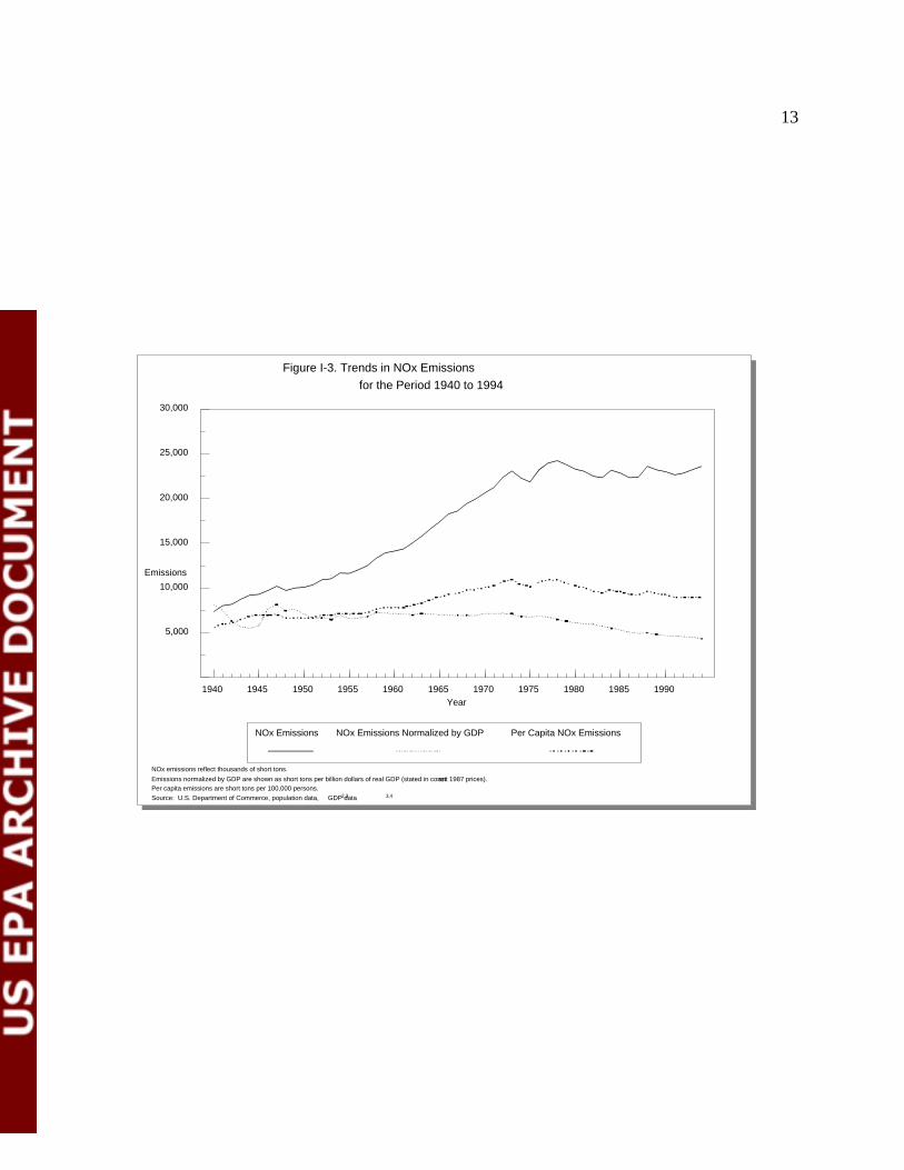
Figure I-3. Trends in NOx Emissions

for the Period 1940 to 1994

1940 1945 1950 1955 1960 1965 1970 1975 1980 1985 1990

5,000

10,000

15,000

20,000

25,000

30,000

Year

Emissions

NOx Emissions NOx Emissions Normalized by GDP Per Capita NOx Emissions

NOx emissions reflect thousands of short tons.

Emissions normalized by GDP are shown as short tons per billion dollars of real GDP (stated in constant 1987 prices).Per capita emissions are short tons per 100,000 persons.

Source: U.S. Department of Commerce, population data, GDP data2,3 3,4

13

14

Organization of this DocumentThis document is organized in 5 major sections: Introduction/Overview, Clean Air Act

Programs Involving Decreases in NO Emissions, Additional Public Health and Environmentalx

Impacts from NO Emissions, Interprogram Issues, and Appendices. The introduction/overviewx

section outlines the purpose of the document and provides information on atmospheric Ncompounds, sources of NO emissions, and trends in emissions of NO . The Programs sectionx x

covers the impact of NO emissions in each of the following subjects: acid deposition, NO , O ,x 2 3

PM, and visibility protection. Drinking water, eutrophication, global warming, stratospheric O3

depletion, terrestrial ecosystems, and toxics products are covered under the additional publichealth and environmental impacts section. A subsequent section covers specific issues stemmingfrom interaction among the various programs, including local and regional NO concerns, seasonalx

controls, interface with the VOCs control program, EPA’s Clean Air Power Initiative, and cross-cutting issues related to the new standards for O and PM. Finally a set of appendices provides3

some detail on the EPA activities within the various programs that impact NO emissions,x

information on sources and sinks of NO emissions, and a listing of acronyms and abbreviationsx .

References

Aneja, Viney P., “Workshop on the Intercomparison of Methodologies for Soil NO Emissions:x

Summary of Discussion and Research Recommendations,” Journal of Air and WasteManagement Association, vol. 44, August 1994.

Chameides, W.L. and E.B. Cowling, The State of the Southern Oxidant Study (SOS): Policy-Relevant Findings in Ozone Pollution Research, 1988-1994. North Carolina State University,April 1995.

National Research Council, Committee on Tropospheric Ozone Formation and Measurement,Rethinking the Ozone Problem in Urban and Regional Air Pollution, National Academy Press,1991.

Schlesinger, W. H. and A. E. Hartley, “A Global Budget for Atmospheric NH ,” Biochemistry 15:3

191-211, 1992.

U.S. Environmental Protection Agency, Control Techniques for Nitrogen Oxides Emissions fromStationary Sources--Revised Second Edition, EPA-450/3-83-002, January 1983.

U.S. Environmental Protection Agency, Office of Air Quality Planning and Standards, NationalAir Pollutant Emission Trends, 1900-1994, October 1995.

15

II. Clean Air Act Programs Involving Decreases in NitrogenOxides (NO ) Emissionsx

A. Acid Deposition

1. Goals of the Program

The primary goal of the Acid Deposition NO Emission Reduction Program is to decreasex

the multiple adverse environmental and human health effects of NO , a principal acid depositionx

precursor that contributes to air and water pollution, by substantially decreasing annual emissionsfrom coal-fired power plants. Electric utilities are a major contributor to NO emissionsx

nationwide: in 1980, they accounted for 30 percent of total NO emissions and, from 1980 tox

1990, their contribution rose to 32 percent of total NO emissions. Approximately 85 percent ofx

electric utility NO emissions comes from coal-fired plants.x

"Acid deposition" occurs when airborne acidic or acidifying compounds, principallysulfates (SO ) and nitrates (NO ) , which can be transported over long distances, return to the4 3

2- -

earth through rain or snow ("wet deposition"), through fog or cloud water (“cloud deposition”),or through transfer of gases or particles (“dry deposition"). While the severity of the damagedepends on the sensitivity of the receptor, acid deposition, according to section 401(a)(1) of theCAA, "represents a threat to natural resources, ecosystems, visibility, materials, and publichealth."

Since NO emissions from the burning of fossil fuels at electric utility power plantsx

contribute to the formation of ground-level O and nitrate PM in the air, ambient levels of NO3 2

and peroxyacetal nitrate (PAN) gases, and atmospheric N deposition, the Acid Deposition NOx

Emission Reduction Program will also mitigate the negative health and welfare effects describedin the other sections of this document. Benefits associated with NO emissions decreases underx

the Acid Deposition Program include lowering excessive N loadings to N sensitive estuarine orcoastal water systems ranging from the Gulf of Maine to North Carolina’s Albemarle PamlicoSound to Florida’s Tampa and Sarasota Bays, decreasing O transported into and within O3 3

nonattainment areas, decreasing inhalable fine particles, and improving visibility, as well asreducing acid deposition damage to lakes and streams, forests and vegetation, and sensitivematerials and structures.

2. Status of the Program

Title IV (Acid Deposition Control) of the CAA specifies a two-stage program fordecreasing NO emissions from existing coal-fired electric utility power plants. Analogous to thex

national allowance program for decreasing sulfur dioxide (SO ) emissions, this program is to be2

16

170 Phase I units known as Table 1 units and 107 Phase II units that have become substitution units. (The1

170 Table 1 units are coal-fired units with Group 1 boilers listed in Table 1 of 40 CFR 73.10 (a) of the Acid RainProgram Regulations.)

implemented in two phases. Phase I affected units (277 boilers) are required to meet the1

applicable annual emission rates beginning with calendar year 1996; Phase II affected units (775boilers) are required to meet the applicable annual emission rates beginning with calendar year2000. Implementation of the first stage of the program, promulgated April 13, 1995 (60 FR18751), will decrease annual NO emissions in the United States by over 400,000 tons per yearx

between 1996 and 1999 (Phase I) and by approximately 1.17 million tons per year beginning in2000 (Phase II). These reductions are achieved by applying low NO burner (LNB) technology tox

dry bottom wall-fired boilers and tangentially fired boilers (Group 1).

The second stage of the program, promulgated December 19, 1996 (61 FR 67112),provides for additional annual NO emissions reductions in the United States of approximatelyx

890,000 tons per year beginning in the year 2000 (Phase II). Taken together, the two stagesprovide for an overall decrease in annual NO emissions in the United States of approximatelyx

2.06 million tons per year beginning in the year 2000. In the second stage of the title IV ProgramEPA has: (1) determined that more effective low NO burner (LNB) technology is available tox

establish more stringent standards for Phase II, Group 1 boilers than those established for Phase I;and (2) established limitations for other boilers known as Group 2 (wet bottom boilers, cyclones,cell burner boilers, and vertically fired boilers), based on NO control technologies that arex

comparable in cost to LNBs.

17

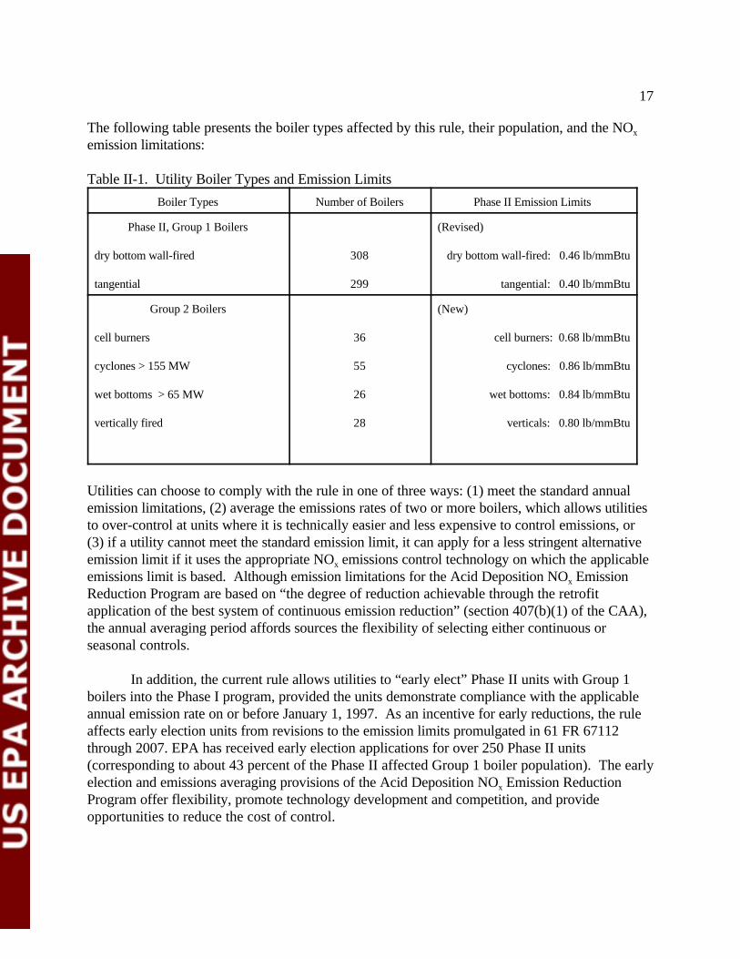
The following table presents the boiler types affected by this rule, their population, and the NOx

emission limitations:

Table II-1. Utility Boiler Types and Emission Limits

Boiler Types Number of Boilers Phase II Emission Limits

Phase II, Group 1 Boilers (Revised)

dry bottom wall-fired 308 dry bottom wall-fired: 0.46 lb/mmBtu

tangential 299 tangential: 0.40 lb/mmBtu

Group 2 Boilers (New)

cell burners 36 cell burners: 0.68 lb/mmBtu

cyclones > 155 MW 55 cyclones: 0.86 lb/mmBtu

wet bottoms > 65 MW 26 wet bottoms: 0.84 lb/mmBtu

vertically fired 28 verticals: 0.80 lb/mmBtu

Utilities can choose to comply with the rule in one of three ways: (1) meet the standard annualemission limitations, (2) average the emissions rates of two or more boilers, which allows utilitiesto over-control at units where it is technically easier and less expensive to control emissions, or(3) if a utility cannot meet the standard emission limit, it can apply for a less stringent alternativeemission limit if it uses the appropriate NO emissions control technology on which the applicablex

emissions limit is based. Although emission limitations for the Acid Deposition NO Emissionx

Reduction Program are based on “the degree of reduction achievable through the retrofitapplication of the best system of continuous emission reduction” (section 407(b)(1) of the CAA),the annual averaging period affords sources the flexibility of selecting either continuous orseasonal controls.

In addition, the current rule allows utilities to “early elect” Phase II units with Group 1boilers into the Phase I program, provided the units demonstrate compliance with the applicableannual emission rate on or before January 1, 1997. As an incentive for early reductions, the ruleaffects early election units from revisions to the emission limits promulgated in 61 FR 67112through 2007. EPA has received early election applications for over 250 Phase II units(corresponding to about 43 percent of the Phase II affected Group 1 boiler population). The earlyelection and emissions averaging provisions of the Acid Deposition NO Emission Reductionx

Program offer flexibility, promote technology development and competition, and provideopportunities to reduce the cost of control.

18

3. Science of NO and Acid Depositionx

The burning of fossil fuels is a major contributor to the formation of NO and thus tox

atmospheric N deposition. "Atmospheric N deposition" is the process by which N in airborne oratmospheric N compounds is transferred to water, soil, vegetation, and other materials (e.g.buildings, statues, automobiles, etc.) on the earth. While some amount of N deposition can bebeneficial for growth of crops and forests, deposition in excess of plant and microbial demand candisturb the soil and water N cycle and can result in acidification of lakes, streams, and soils as wellas eutrophication of estuarine and coastal waters bodies (Paerl, 1993) and, more rarely,freshwater ecosystems (Church, 1997:17; Vitousek et al, 1997:10). Eutrophication of estuarineand coastal waters is addressed in section III.B of this document.

As mentioned previously, “acid deposition” involves acidic and acidifying sulfur and Ncompounds, which can be transported over short and long distances, thus affecting naturalresources and materials up to hundreds of kilometers from the sources of precursor emissions(SO and NO ). As with NO emissions and O formation, the relationship between precursor2 x x 3

emissions and acidity in the atmosphere is complex (NAPAP, 1993:23). Some of these acidic andacidifying compounds are not emitted directly during the burning of fossil fuels; they are formedby chemical conversions in the atmosphere of SO and NO gases released during combustion.2 x

a. AcidificationAcidification effects are related to increases in the acidity of water and soil in ecosystems.

Increases in water acidity can impair the ability of certain types of fish and other biota to grow, reproduce, and hence, survive. In some acidified lakes and streams, entire populations of fishspecies have disappeared. For example, many lakes in the higher Adirondack mountains of NewYork and many streams in the Appalachian mountain region have experienced loss of trout andother biodiversity losses due to high acidity levels in the water (NAPAP, 1993:76). Increases insoil acidity can impair the ability of some types of trees to grow and resist disease. For example,growth reductions and injury to red spruce on high elevation ridges of the Appalachian mountainsfrom Maine to Georgia have been linked to nutrient leaching caused by high soil acidity anddeposition and primarily linked to a predisposition to frost damage from highly acidic cloud water(Johnson et al, 1992). The effects of acid deposition on forested ecosystems is an importantresearch issue primarily because the observational data are inclusive (i.e., trees react very slowlyto damaging influences).

i. Lakes, Streams, and Watershed EcosystemsRecent scientific studies indicate the amount of N that can be sequestered and retained in

certain watersheds by biological processes is limited (US EPA, 1995:11). As these watershedsmove towards N saturation, nitrate and, to a lesser extent, nitrite can begin to leach into surfacewaters, accelerating the process of long-term chronic acidification. Adding N to freshwaterecosystems that are rich in phosphorus can eutrophy as well as acidify the waters. Eutrophicationalso leads to decreased diversity of both plant and animal species (Vitousek et al, 1997:10).

Atmospheric deposition of N compounds plays a significant role in short-term episodic

19

acidification, which occurs when pulses of highly acidic water enter lakes and streams duringstorm flow, spring snowmelt or autumn rains after prolonged summer drought. Acidic episodescan expose aquatic organisms (e.g., fish, amphibians) to "acid pulses" containing highconcentrations of inorganic monomeric aluminum (Al ), which is highly toxic to fish, often duringim

the spawning season in the Spring. Episodic acidification can affect poorly buffered surfacewaters in many regions, including high elevation areas in the Mid-Atlantic and the West, as well asthe Northeast (US EPA, 1995:14, 25).

The relative contributions of N and sulfur compounds, primarily NO and SO , to the3 4- 2-

problem of surface water and soil acidification differs among regions and sites. The relativecontributions depend not only on external differences in the deposition rates of these chemicals,but also on differences among the capacities of receptor watersheds to retain N and sulfur and to“buffer” against pH changes (i.e. alkalinity or hardness). Many areas in the West are moreaffected by N deposition, particularly dry deposition, than by sulfur deposition (US EPA,1995:56).

Acidified watershed ecosystems can show signs of recovery following decreases in aciddeposition rates. According to the Acid Deposition Standard Feasibility Study (US EPA, 1995),in watersheds where atmospheric deposition of sulfur has been and will continue to be decreased(commensurate with decreases in SO emissions under Title IV of the CAA), environmental2

modeling has projected a range of benefits (i.e., fewer acidic ecosystems) in sensitive ecosystems. The number of acidic systems are substantially fewer than the model projects without the SO2

emissions reductions in Title IV. Recovery rates depend primarily on the rates of pollutantdecreases, ecosystem N retention processes, time lags caused by long-term biological processresponses, and other possible changes in soil chemistry. Although watershed N saturation iswidely accepted in the research community, it is also broadly recognized that there areuncertainties associated with the rate at which a watershed may become N saturated. However,additional NO emissions reductions would likely produce a two-fold benefit by decreasing acidx

deposition rates and lengthening the average time before watersheds reach N saturation.

ii. Forests and VegetationPast assessments of the impacts of acid deposition on forests and vegetation have focused

primarily on SO and sulfur deposition, largely because N is an essential nutrient for many2

biological processes (Atkinson,1993; Sommerville et al, 1989). Because N is commonly used as afertilizer, it was thought that any atmospherically deposited N would be quickly and beneficially incorporated into plant and tree organisms (US EPA, 1995:11). Like aquatic ecosystems, thebiological demand for N in forest ecosystems and other vegetation varies across geographicalareas and by season. It is also highly dependent on factors such as tree/plant species (e.g.,deciduous- species trees tend to have greater demand for N per unit biomass than coniferous-species trees), soil type, forest age, prevalence of disease and other stresses such as extreme coldor drought, and land management practices (e.g., use of fertilizers, liming, or other cultivationmethods) (US EPA, 1995:11).

20

Acidification effects on health and productivity of forests and other vegetation are dividedinto two types: (1) direct effects on foliar organs and (2) indirect or soil-mediated effects resultingfrom acidification and physical/chemical alteration of the soil. Direct acidification effects mightinclude foliar damage, erosion of leaf cuticle waxes, and changes in the physiology of tree leaves(Society of American Foresters, 1984). Soil-mediated acidification effects include toxic effects onroots as well as possible changes in nutrient availability, reproductive and regenerative processes.

Increasing evidence reveals that dry deposition is usually a significant portion of totalatmospheric deposition (wet + cloud + dry) of both sulfur and N. For example, across all sitesincluded in a recent review, dry deposition ranged from 9 to 59 percent of total deposition forsulfur (S), 25 to 70 percent for nitrate, and 2 to 33 percent for ammonia (Lovett, 1994; 629-650). Thus, in many areas N is taken up by foliage primarily in dry chemical form (e.g., as nitricacid vapor), rather than with deposition in precipitation. The response of forest ecosystems todirect effects of atmospheric deposition of both sulfur and N depend on the nature and timing ofthe deposition as well as the type of vegetation exposed. Some species appear less tolerant thanothers (i.e., spruce-fir ecosystems appear to be the most sensitive) and younger trees appear morevulnerable than mature trees.

Considerably more but still limited research has been performed on soil-mediatedacidification effects since soils, together with climate, determine the productivity of terrestrialecosystems. These studies have focused primarily on decreases in available base cation plantnutrients below amounts required for plant growth; and increased mobilization and availability oftoxic aluminum (Al) and other metal ions (Brandt, 1993:14, 31). In certain soils, N depositioncan deplete nutrients by leaching calcium (Ca), magnesium (Mg), and potassium (K). Theseimportant cations are often replaced by hydrogen ions (H ) which, together with increased+

mobilization of aluminum, can greatly increase soil acidification. Significant increases in sulfateand/or nitrate concentration will lead to preferential mobilization, availability, and toxicity ofaluminum over base cations (e.g., Ca , Mg , K ) in soils with low base saturation, such as the2+ 2+ +

soils commonly found in high-elevation sites in the Northeast and Southeast (Turchenek et al.,1987; Turner et al., 1986). Increased concentrations and mobility of aluminum are linked withroot damage and limited uptake of root calcium and magnesium. (Shortle and Smith, 1988).

The timing of aluminum concentration peaks is also important. Toxic aluminum peaksrelated to nitrate fluctuations commonly occur in late summer or early fall when soil temperaturesand root growth are usually high (Joslin et al., 1992). It has been estimated that up to 3 percentof forested soils in the eastern United States could have toxic levels of trace elements in solutionor could act as a source of high levels of acidity to surface waters, thus contributing to theacidification of watershed ecosystems discussed previously. Further, up to 40 percent of easternsoils may be sensitive to changes in nutrient status that could result in reduced forest growth oradditional acidification of surface waters (Turner et al., 1986).

Forest ecosystems and other vegetated regions (e.g. crop and grasslands) are alsosusceptible to adverse excess N loading effects analogous to eutrophication in aquatic ecosystems.

21

These N loading effects result from deposited N of all forms (i.e., including forms other thanacidic nitrate such as ammonia and dissolved organic N) and tend to occur when the demand byplants and heterotrophic soil organisms for N has been substantially satisfied (i.e., the ecosystem isapproaching N saturation). N deposition to forest ecosystems can affect competitive relationshipsacross tree/plant species and can therefore change species composition and/or diversity. Otherpotential adverse N loading effects include decreased uptake of nutrients from soil, increasedsusceptibility to insect and disease attack, and altered reproductive or regenerative processes (USEPA, 1991).

Evidence has accumulated suggesting N availability in certain forest ecosystems are inexcess of plant and microbial demand. Early indicators of N saturation have implications to forestecosystems over large geographic areas. Possible effects include elevated concentrations ofnitrate, aluminum, and hydrogen in streams, which would decrease water quality, increasesusceptibility to frost damage or other disruptions of physiological function that would lowerproductivity in certain forest types, increased cation [nutrient] leaching from soils and nitratelosses that would lead to lower soil fertility and increased acidity (Aber, et al., 1989). Additionally, recent research conducted in the Colorado Front Range demonstrates that highelevation (alpine and subalpine) ecosystems may be nearly N saturated at current levels of Ndeposition. The results suggest that the Colorado Front Range may be an early warning indicatorof N saturation for other high-elevation catchments in the Rocky Mountains and the westernUnited States and an indicator for disruption of N cycling in forested ecosystems at lowerelevations as well. (Williams, et al., 1996)

Results of twelve years of experimental N addition to grassland plots in Minnesota haveshown reductions in grassland biodiversity associated with N loadings. N added to research plotsresulted in the loss of almost all native prairie grass species and to dominance by a weedyquackgrass. These results indicate that N loading can be a major threat to grassland ecosystems,causing loss of diversity, increased abundance of nonnative species, and the disruption ofecosystem functioning. (Wedin, et al., 1996)

Finally, NO is a primary O precursor and the damaging effects of O on forestx 3 3

ecosystems have been studied more comprehensively than those related to excess N loading andacidification. O is the most destructive pollutant in forest ecosystems (deSteiguer et al., 1990). 3

The injurious effects of O on plants include visible damage to foliage, decreased growth of roots3

and shoots, decreased yield, changes in quality of harvest, and changes in susceptibility to otherstresses. (US EPA, 1993).

b. Materials and StructuresThe role of atmospheric N deposition in metals corrosion has not been completely

resolved; some suggest, on the basis of laboratory evidence, that NO appreciably increases thex

corrosive effect of SO (NAPAP, 1993:93-94). It has been estimated that 31-78 percent of the2

dissolution of galvanized steel and copper is attributable to wet and dry acid deposition (NAPAP,1993:93). Deposited acids corrode and dissolve the protective zinc coatings on these surfaces,

22

and as a result, the metal underneath rusts. The specific role of N-based acids in the process hasnot yet been established. In the late 1980s, NAPAP and the Economic Commission for Europeinitiated several projects in the United States and Europe to clarify the scientific foundationlinking acid deposition and materials damage (NAPAP, 1993:93). These projects include researchto investigate the mechanisms by which N deposition directly impacts or works with otherpollutants to damage structural and other materials.

Acid deposition also damages exterior paints applied to wood and metal substrates. Special paint formulations involving different organic and inorganic binders, pigments, andadditives have been developed to resist corrosion and spotting from acid deposition (NAPAP,1993:96). To maximize durability, these special finishes are applied under factory-controlledconditions. The costs to automotive manufacturers for including acid-resistant features have beenestimated by the EPA and NAPAP to be as high as $400 million annually (US EPA, 1995:97). Acid deposition can also accelerate the deterioration of stone through processes of erosion,solubilization, blackening of the stone surface, and cracking (US EPA, 1995:96-97). Acidic-related damage to cultural and historic buildings, monuments, and structures increases annualmaintenance and reparation costs, which can be extensive. Thus, potentially large economicbenefits could be associated with lessened physical materials damage achieved, in part, throughadditional NO emissions reductions.x

4. How much reduction is needed?

Our current knowledge of the science of NO and acid deposition does not supportx

quantitative assessments of the tons of NO needed beyond the CAA nationally or by region tox

protect sensitive aquatic and forest ecosystems or to reduce acidic-related damage to materials,structures, and cultural or historic resources. Nonetheless, model projections from EPA’s recentAcid Deposition Standard Feasibility Study (October 1995) indicate that N deposition may playan important role in ongoing and future acidification of sensitive watershed ecosystems, and mayequal or exceed the effects of sulfur deposition. The extent of potential future effects depends onhow rapidly atmospheric N deposition moves watersheds toward a state of N saturation, i.e.,where input of N exceeds biological uptake of N on an annual basis. The time to watershed Nsaturation will vary depending on forest age, historic and future rates of N deposition, futurechanges in ambient temperatures, water stress, land use as well as other variables.

The United States Congress directed EPA, in Section 404 (Acid Deposition StandardsStudy) of the CAA, to provide a report on the feasibility and effectiveness of an acid depositionstandard or standards to protect sensitive and critically sensitive aquatic and terrestrial resources. The EPA’s Acid Deposition Standard Feasibility Study: Report to Congress (US EPA, 1995)fulfills this requirement by integrating state-of-the-art ecological effects research, emissions andsource receptor modeling, and evaluation of implementation and cost issues related to thefeasibility of establishing and implementing an acid deposition standard or standards.

An acid deposition standard is a rate of deposition (most likely in units of kilograms of

23

A hectare is a unit of surface measure equal to 10,000 square meters.2

pollutant per hectare per year) that provides a predetermined amount of protection to specific2

ecological resources. Aquatic systems are the natural resources most at risk from acid depositionand those most amenable to quantitative assessment. Other ecological resources such as high-elevation red spruce forests in the eastern United States and Canada may also be at risk, but less isknown about the effects process, and the rate and extent of impacts on those resources. Targetpopulations of Adirondack lakes, Mid-Atlantic streams, and Southern Blue Ridge streams wereselected as case studies for detailed analysis in the Acid Deposition Standard Feasibility Studybecause they represent ecosystems that receive fairly high amounts of acid deposition, aresensitive to acid deposition, have the best historical data, and have been the focus of scientificstudies. While many surface waters in western North America are as sensitive as, or moresensitive than, aquatic systems in the East, acid deposition rates in the West are currentlysufficiently low that the risk of chronic (long-term) acidification to resources in the West is lowand is expected to remain low for the next 50 years. Episodic acidification from spring snowmelts, which adversely affects some eastern surface waters, also affects high elevation westernsurface waters. (US EPA, 1995:xiv).

For the Acid Deposition Standard Feasibility Study, EPA scientists modeled the potentialcombined effects of atmospheric deposition of both sulfur and N on the chemistry of acid-sensitive lakes and streams in the regions selected for in-depth study: Adirondacks, Mid-Appalachian Region, and Southern Blue Ridge Province. Model simulations projected waterchemistry responses out to the year 2040. Projections of sulfur and N deposition rates werebased on results expected from implementation of the 1990 CAA amendments as well as othermore restrictive deposition reduction scenarios using EPA’s Regional Acid Deposition Model(RADM). The modeling incorporated a decision-model based estimate of SO emission2

allowance trading and the Canadian SO control program. Explicit watershed models and data to2

estimate the times required for watersheds to reach N saturation were unavailable at the time ofthe Study therefore, EPA scientists assumed an encompassing range of times (50 years, 100 years,250 years, and never) to watershed N saturation and then estimated the potential consequenteffects on surface water Acid Neutralizing Capacity (ANC). (ANC is a commonly used measureof the concentration of dissolved compounds [e.g., carbonate, bicarbonate, borates, and silicates]in fresh water which collectively tend to create less acidic conditions. Surface waters with higherANC are generally more resistant to acidification.) This innovative modeling component of theAcid Deposition Standard Feasibility Study is referred to as the Nitrogen Bounding Study (NBS)in that, given the uncertainties associated with the time when a watershed may reach N saturation,the results effectively bounded the range of possible water chemistry outcomes . The NBSreceived external technical peer review and the entire Feasibility Study has been peer-reviewed byEPA’s Science Advisory Board (US EPA, Appendix D, 1995).

Although model projections in the Acid Deposition Standard Feasibility Study are forthree specific target populations, i.e., groups of lakes or streams with watersheds of similar size,land, and other characteristics, not even for all watersheds in the study regions, they signal a

24

Observational data (currently being collected and analyzed by the New York State Department of3

Environmental Conservation) which compare the amount of nitrate falling on several Adirondack watersheds with theamount of nitrate leaving these watersheds in stream water indicate the watersheds may be nearing N saturation(Simonin, 1996; Evans et al., 1996).

direction of probable need for substantial additional reductions in year-round NO emissions in thex

Eastern United States For example, it was estimated that a 40-50 percent decrease in SO and2

NO emissions beyond the CAA may be required to keep the number of chronically acidified lakesx

in the Adirondacks at 1984 proportions, if these watersheds move towards N saturation in 100years (US EPA, 1995:xvi). Without additional emissions reductions, the model projects the3

number of acidic lakes in the Adirondacks could increase by almost 40 percent by 2040, if thesewatersheds move towards N saturation in 100 years. As described, the modeling effortencompasses a range of responses based on time to N watershed saturation. For example, in thecase in which saturation never occurs in the Adirondacks, the number of acidified lakes is loweredby 40 percent due to the SO emissions reduction in the CAA. The effects on episodic2

acidification of lakes and streams would be even more pronounced as it is now understood thathigh nitrate levels are largely responsible for acidic episodes during snowmelt and high streamflow periods in the Northeast and probably high-elevation areas in other regions of the UnitedStates (Wigington et al., 1996; US EPA, 1995).

Recent results from the Bear Brook Watershed Manipulation Experiment illustrate therapidity with which forested watersheds in the Northeast may reach N saturation in response toincreased atmospheric N deposition (Scofield, 1995; Norton et al., 1994). :. Increased leaching ofnitrate from forested catchments into streams or lakes could lead to increases in surface wateracidification in some areas that could offset increases in ANC (i.e., reductions in acidity) expectedfrom decreases in SO emissions under the CAA. 2

5. How much reduction will be achieved with current andprojected Title IV programs?

Under the current rule for the Acid Deposition NO Emission Reduction Program (40x

CFR Part 76; FR 18751, April 13, 1995), NO emissions from existing coal-fired electric utilityx

power plants will be decreased by over 400,000 tons per year between 1996 and 1999 (Phase I)and by over 1.5 million tons per year beginning in 2000 (Phase II). These decreases are achievedby 857 dry bottom wall-fired and tangentially fired boilers (Group 1). The annual cost of thisregulation to the electric utility industry is estimated as $267 million (in 1990 dollars), resulting inan overall cost-effectiveness of $227 per ton of NO removed. The nationwide cost impact onx

electricity consumers is an average increase in electricity rates of approximately 0.21 percent,beginning in 2000 (61 FR 1442).

The Phase II Acid Deposition NO Emission Reduction Program will achieve an additionalx

reduction of 890,000 tons of NO per year from existing coal-fired electric utility power plantsx

beginning in 2000. One hundred twenty thousand (120,000) tons would come from lowering the

25

emission limits for 580 Group 1 boilers affected in Phase II; 77 percent of these boilers arelocated in the Eastern United States, defined by the 37 states adjacent to and east of theMississippi River. The additional tons would come from establishing emission limits for 190 high-emitting Group 2 boilers (i.e., cell burners, cyclones, wet bottom boilers, and vertically firedboilers); 89 percent of these boilers are located in the Eastern United States.

The Phase II Acid Deposition NO Emission Reduction Program appears to represent ax

singular regulatory opportunity for controlling high-emitting Group 2 boilers, which typically emitNO at rates in excess of 1.0 lb/mmBtu. The majority of these coal-fired boilers are locatedx

outside designated O nonattainment areas in the states of Illinois, Indiana, Kentucky, Michigan,3

Missouri, Ohio, and West Virginia. EPA modeling analyses show that transport of O and O3 3

precursors (primarily NO ) from upwind areas in the Eastern United States contributesx

significantly to O exceedances in virtually all nonattainment areas in the Northeast Ozone3

Transport Region (60 FR 45583). Further, simulations on EPA's Regional Acid DepositionModel (RADM) indicate not only that utility sources of N contribute the majority of deposits onthe western side of the Chesapeake Bay, but also that the areal extent of the Chesapeake Bayairshed (which encompasses all or parts of Indiana, Kentucky, Ohio, and West Virginia as well as10 other states) underestimates the areas contributing atmospheric sources of N depositionentering the Bay (Dennis, 1995).

The average cost-effectiveness of utility NO controls under the rule compares favorablyx

to many of the other pollution control measures being considered by states to mitigate persistentO nonattainment and/or N-based eutrophication water quality problems. For example, decreases3

in NO emissions from coal-fired power plants are comparable or less expensive to implementx

than certain alternative controls for reducing N loadings to the Chesapeake Bay from area sources(farms, forests), even without counting the “clean air” benefits associated with the NO emissionx

reductions. Such alternatives, as well as others in the mobile source sector, are presently beingconsidered by Maryland, Virginia, Pennsylvania, and the District of Columbia to achieve the 40percent-decrease in controllable nutrient supplies to the Bay, to which these jurisdictions havecommitted. The average cost-effectiveness of these other controls are: chemical addition orbiological removal of N from wastewater processing ($4,000 to over $20,000/ton N removed)and "management practices" to decrease N from fertilizers, animal waste, and other nonpointsources ($1,000 to over $100,000/ton of N removed) (Camacho, 1993; Shuyler, 1992). While itis recognized that to address the Bay's excessive nutrient loading problem in the most efficientmanner requires pursuing an integrated strategy of air, water, and agricultural pollution controlpractices, these relative cost-effectiveness ratios and modeling analyses suggest the additionalNO emissions reductions from coal-fired power plants in the acid deposition rule are a criticalx

component of this strategy.

6. Summary

The primary goal of the Acid Deposition NO Emission Reduction Program is to reducex

the multiple adverse effects of NO , a principal acid deposition precursor that contributes to airx

and water pollution, by substantially decreasing annual emissions from existing coal-fired power

26

Known as Table 1 units. These 170 units represent the coal-fired units with Group 1 boilers that are listed in4

Table 1 of 40 CFR 73.10 (a) of the Acid Rain Program Regulations and are subject to 40 CFR Part 76, Acid Rain NOx

Emission Reduction Rule.

plants. Acid deposition occurs when airborne acidic and acidifying compounds, principally sulfates(SO ) and nitrates (NO ), which can be transported over long distances, return to the earth4 3

2- -

through rain or snow ("wet deposition"), through fog or cloud water (“cloud deposition”), orthrough transfer of gases or particles ("dry deposition"). According to section 401(a)(1) of theCAA, acid deposition "represents a threat to natural resources, ecosystems, visibility, materials,and public health." Since NO emissions from the burning of fossil fuels at power plants alsox

contribute to the formation of ground-level O and nitrate PM in the air, ambient levels of NO ,3 2

and excessive N loadings to the Chesapeake Bay and other estuaries, decreases in NO emissionsx

under the Acid Deposition Program are expected to have multiple and synergistic beneficialimpacts on public health and welfare.

The Acid Deposition NO Emission Reduction Program consists of a two-stage programx

which, analogous to the Acid Deposition allowance program for SO emission reduction, is2

implemented in two phases. The first stage of the program, authorized by section 407(b)(1) ofthe CAA and implemented pursuant to 40 CFR Part 76, promulgated in April 1995, will decreaseannual NO emissions by over 400,000 tons per year, beginning in 1996, from 170 Phase Ix

affected units with Group 1 boilers (i.e., dry bottom wall-fired boilers and tangentially fired4

boilers). An additional NO emissions reduction of over 200,000 tons per year will probably bex

realized, beginning in 1997, from about 250 “early election” Phase II units with Group 1 boilerswhich voluntarily opted into the Phase I program. The total NO emissions reduction that wouldx

be achieved by applying LNB technology under the April 13, 1995 rule is estimated at about 1.2million tons per year, beginning in 2000.

In December 1996, EPA promulgated regulations for implementing the second stage ofthe program, authorized by section 407(b)(2) of the CAA. Compliance with the rule wouldachieve an additional NO emissions reduction of 890,000 tons per year, beginning in 2000, fromx

existing coal-fired units affected in Phase II. Seventy-seven percent of the Group 1, Phase IIboilers and 89 percent of the Group 2 boilers are located in states adjacent to or east of theMississippi River. EPA modeling analyses show that utility sources of N in this 37-state regioncontribute significantly to the acidification of certain watershed ecosystems (US EPA, 1995),excess N deposits to the Chesapeake Bay (Dennis, 1995), and O exceedances in virtually all3

nonattainment areas in the densely populated Northeast Ozone Transport Region (60 FR 45583).The total NO emissions decrease under the statutory authority of Title IV (Acid Depositionx

Control) is estimated at about 2 million tons per year, beginning in 2000.

Such emissions decreases may not be adequate, however, to protect sensitive watershedecosystems in the Northeast and Mid-Atlantic regions as well as in high-elevation areas in theWest and other regions. Recent model projections from EPA’s Acid Deposition StandardFeasibility Study: Report to Congress (US EPA, 1995) signal a direction of probable need for

27

substantial additional reductions in year-round NO emissions. For example, it was estimated thatx

a 40-50 percent decrease in SO and NO emissions beyond the CAA may be required to keep the2 x

number of chronically acidified lakes in the Adirondacks at 1984 proportions, if the time to Nsaturation in these watersheds is 100 years or less. Without additional emissions reductions, themodel projects the number of acidic lakes in the Adirondacks could increase by almost 40 percentby 2040, assuming N saturation in 100 years. There are uncertainties associated with determiningthe rate at which a watershed may reach N saturation and therefore the EPA’s Study provides arange of possible responses. However, the magnitude and direction of projected responses pointtowards a need for further emissions reductions to protect sensitive ecosystems. The negativeeffects of no additional emissions reductions could be even more pronounced on episodicacidification of lakes and streams in the Northeast (and potentially high-elevation areas in otherregions) where high nitrate levels are largely responsible for acidic episodes during snowmelt andhigh stream flow periods (Wigington et al., 1996; US EPA, 1995). Thus, wintertime NOx

emissions reductions are especially important to lessening the incidence and severity of acidicepisodes in certain areas. Continuous year-round NO controls appear to be the most beneficialx

for decreasing acid deposition damage to natural resources.

References

Aber, John D., Knute J. Nadelhoffer, Paul Steudler, and Jerry M. Melillo. 1989. “NitrogenSaturation in Northern Forest Ecosystems.” BioScience Vol. 39 No. 6. June.

Atkinson, Giles. 1993. “The Impact of Acid Rain on Crops.” Reprint from Center for Social andEconomic Research on the Global Environment, University College London and University ofEast Anglia, UK.

Brandt, C. Jeffrey. 1994. Acidic Deposition and Forest Soils: Potential Changes in NutrientCycles and Effects on Tree Growth. Battelle Pacific Northwest Laboratory. EPA 600/R-94/153ERL-COR 817. May.

Camacho, R. 1993. “Financial Cost-Effectiveness of Point and Nonpoint Source NutrientReduction Technologies in the Chesapeake Bay Basin.” Report No. 8 of the Chesapeake BayProgram Nutrient Reduction Strategy Reevaluation. Washington, DC. U.S. EnvironmentalProtection Agency, February.

Church, M.R. 1997. “Hydrochemistry of forested catchments.” Annual Reviews of Earth andPlanetary Sciences. Vol. 25 (preprint).

de Steiguer, J.E., J.M. Pye, and C.S. Love. 1990. “Air pollution damage to U.S. forests.” Journal of Forestry, Vol. 88, No. 8, p. 17. August.

Evans, C.D., T.D. Davies, P.J. Wigington, M. Tranter, and W.A. Kreiser. 1996 (in press). “Useof factor analysis to investigate processes controlling the chemical composition of four streams inthe Adirondack mountains,” New York. Journal of Hydrology.

28

Federal Register. 1995. 40 CFR Part 76. “Acid Rain Program: Nitrogen Oxides EmissionReduction Program.” Vol. 60, No. 71, pp. 18751. Thursday, April 13, 1995. Direct final rule.

Federal Register. 1995. 40 CFR, Parts 80, 86 and 89. “Control of Air Pollution From Heavy-Duty Engines.” Vol. 60, No. 169, pp. 45580. Thursday, August 31, 1995. Proposed rule.

Federal Register. 1996. 40 CFR Part 76. “Acid Rain Program: Nitrogen Oxides EmissionReduction Program.” Vol. 61, No. 13, pp. 1442. Friday, January 16, 1996. Proposed rule .

Johnson, A.H., S.B. McLaughlin, M.B. Adams, E.R. Cook, D.H. DeHayes, C. Eager, I.J.Fernandez, D.W. Johnson, R.J. Kohut, V.A. Mohnen, NM.S. Nicholas, D.R. Peart, G, A. Schier,and P.S. White. 1992. “Synthesis and Conclusions from Epidemiological and MechanisticStudies of Red Spruce Decline.” Pp. 385-412. In C. Eager and M.B. Adams, eds. Ecology andDecline of Red Spruce in the Eastern United States. Springer Verlag, New York.

Joslin, J.D., J.M. Kelly, and H. Van Meigroet. 1992. “Soil chemistry and nutrition of NorthAmerican spruce-fir stands: evidence for recent change.” J. Environ. Qual. 21:12-30.

Lovett, G.M. 1994. “Atmospheric deposition and pollutants in North America: an ecologicalperspective.” Environmental Applications 4:629-650.

National Acid Precipitation Assessment Program (NAPAP). 1990. Integrated Assessment . External Review Draft.

“National Acid Precipitation Assessment Program (NAPAP).” 1992 Report to Congress. June1993.

Norton, S.A., J.S. Kahl, I.J. Fernandez, L.E. Rustad, J.P. Scofield and T.A. Haines. 1994. “Response of the West Bear Brook Watershed, Maine, USA, to the addition of (NH ) SO : 3-4 2 4

year results.” Forest Ecology and Management. 68:61-73.

Paerl, H.W. 1993. “The Emerging Role of Atmospheric Nitrogen Deposition in CoastalEutrophication: A Biogeochemical and Trophic Perspective.” Canadian Journal of Fisheries andAquatic Sciences. 50:2254-2269.

Scofield, J.P. 1995. “Annual Progress Report for Cooperative Agreement CR-816261. Watershed Manipulation Project: Maine Site Group.”

Shortle, W.C. and K.T. Smith. 1988. “Aluminum-induced calcium deficiency syndrome indeclining red spruce.” Science 240:1017-1018.

Shuyler, L.R. 1992. “Cost Analysis for Nonpoint Source Control Categories in the ChesapeakeBasin.” Annapolis, MD: U.S. Environmental Protection Agency . Chesapeake Bay Program.

29

March.

Simonin, H.A. 1996. Unpublished data.

Society of American Foresters. 1984. “Acidic Deposition and Forests.” Bethesda, MD.

Sommerville, M.C., S.E. Spruill, J.O. Rawling, and V.M. Lesser. 1989. “Impact of Ozone andSulfur Dioxide on the Yield of Agricultural Crops.” Technical Bulletin 292. North CarolinaAgricultural Research Service, North Carolina State University. November.

Taylor, G.E., D.W. Johnson, and C.P. Anderson. 1994. “Air pollution and forest ecosystems: aregional to global perspective.” Ecological Applications. 4:662-689.

Turchenek, L.W., S.A. Abboud, C.J. Tomas, R.J. Fessenden, and N. Holowaychuck. 1987. “Effects of acid deposition on soils in Alberta.” Acid Deposition Research Program, Calgary,Alberta, Canada.

Turner, R.S., R.J. Olson, and C.C. Brandt. 1986. “Areas having soils characteristics that mayindicate sensitivity to acidic deposition under alternative forest damage hypotheses.” ORNL/TM-9917. Environmental Sciences Division. Pub. No. 2720. Oak Ridge National Laboratory . US EPA. 1991. “Air Quality Criteria for Oxides of Nitrogen: External Review Draft,” EPA600/8-91/049bA, Environmental Criteria and Assessment Office, Office of Health andEnvironmental Assessment, Research Triangle Park, NC. August.

US EPA. 1993. Air Quality Criteria for Ozone and Related Photochemical Oxidants. VolumeII of III. EPA 600/Ap-93/004d. April.

US EPA. 1995. Acid Deposition Standard Feasibility Study: Report to Congress. EPA 430-R-95-001a. October.

Vitousek, P.M., J. Aber, R.W. Howarth, G.E. Likens, P.A. Matson, D.W. Schindler, W.H.Schlesinger, and G.D. Tilman, “Human Alteration of the Global Nitrogen Cycle: Causes andConsequences,” Issues in Ecology, Number 1, Spring 1997.

Wedin, David A. and David Tilman. 1996. “Influence of Nitrogen Loading and SpeciesComposition on the Carbon Balance of Grasslands.” Science, Vol 274, December 6, 1996.

Wigington, J.P, D.R. DeWalle, P.S. Murdoch, W.A. Kretser, H.A. Simonin, J. Van Sickle, andJ.P. Baker. 1996 (in press). “Episodic acidification of small streams in the Northeastern UnitedStates II. Ionic controls of episodes.” Ecological Applications 6(2).

Williams, Mark W., Jill S. Baron, Nel Caine, Richard Sommerfield and Robert Sanford, Jr. 1996.

30

“Nitrogen Saturation in the Rocky Mountains.” Environmental Science & Technology Vol 30 No2.

31

B. Nitrogen Dioxide

1. Goal of the Program

The EPA has established national ambient air quality standards (NAAQS) for nitrogendioxide (NO ) designed to protect public health and welfare. The goal of the program is to first2

achieve these clean air standards throughout the country and then to maintain the standards. Control of NO emissions is needed locally in some areas to continue to maintain the NOx 2

NAAQS.

2. Status of the Program

Section 109 of the CAA directs the EPA Administrator to propose and promulgateprimary and secondary NAAQS for pollutants identified under section 108. Section 109 defines aprimary standard as that necessary to protect the public health, allowing an adequate margin ofsafety. A secondary standard, as defined in section 109, must specify an air quality concentrationneeded to protect the public welfare from any known or anticipated adverse effects associatedwith the presence of the pollutant in the ambient air. Welfare effects, as defined in section 302(h)of the CAA include, but are not limited to, effects on soils, water, crops, vegetation, materials,animals, wildlife, weather, visibility and climate, damage to and deterioration of property, andhazards to transportation, as well as effects on economic values and on personal comfort andwell-being.

States are primarily responsible for ensuring attainment and maintenance of the NAAQS.Under title I of the CAA, States are to submit, for EPA approval, State implementation plans(SIPs) that provide for the attainment and maintenance of such standards through controlprograms directed to sources of the pollutants involved. In addition, Federal programs providefor nationwide reductions in emissions of air pollutants through, for example, the Federal MotorVehicle Control Program, which involves controls for automobile, truck, bus, motorcycle, andaircraft emissions.

The primary and secondary NAAQS for NO is 0.053 parts per million (ppm) (1002

micrograms per meter cubed) annual arithmetic average. In selecting the concentration for thecurrent standard, the Administrator made judgments regarding the lowest concentrations at whicheffects were observed, sensitive populations, nature and severity of public health effects, andmargin of safety. After assessing the evidence, the Administrator concluded that the annualstandard of 0.053 ppm adequately protected against adverse health effects associated withlong-term exposures and provided some measure of protection against possible short-term healtheffects. The June 19, 1985 Federal Register notice (50 FR 25532) provides a detailed discussionof the bases for the existing standard.

32

Currently, all areas of the United States are in attainment of the annual NO NAAQS of2

0.053 ppm (EPA, 1994). Los Angeles is the only city in the United States to record violations ofthe annual average NO NAAQS during the past decade. In 1992, Los Angeles reported air2

quality measurements which met the NO NAAQS for the first time. 2

In accordance with the provisions of sections 108 and 109 of the CAA, as amended, theEPA conducted a review of the criteria upon which the existing NAAQS for NO are based. The2

revised criteria were published simultaneously with the issuance of the October 11, 1995 FederalRegister notice of proposed rulemaking on the NO NAAQS (60 FR 52874). After evaluating the2

revised health and welfare criteria under section 109(d)(1) of the Act, and considering publiccomment, the Administrator published a final rulemaking notice on October 8, 1996 (61 FR52852) which concludes that it is not appropriate to propose any revisions to the primary andsecondary NAAQS for NO at this time. As described in the proposed and final rulemaking2

notices, EPA determined that a 0.053 ppm annual standard would keep annual NO2

concentrations considerably below the long-term levels for which serious chronic effects havebeen observed in animals. Retaining the existing standard also provides protection againstshort-term peak NO concentrations at the levels associated with mild changes in pulmonary2

function and airway responsiveness observed in controlled human studies.

3. Science of NO2

NO2

NO is a brownish, highly reactive gas that is formed in the ambient air through the2

oxidation of NO. As described in the “Ozone” section, emissions of NO play a major role in theformation of O in the lower atmosphere through a complex series of reactions with VOCs. 3

Emissions of NO are rapidly oxidized in the atmosphere to NO . NO refers to the sum of NO2 x 2

and NO. Sources of NO (NO ) emissions are described in the “Introduction/Overview” sectionx

and Appendix C. The major sources of anthropogenic NO emissions are on-road vehicles andx

electric utilities.

Health Effects of Concern.Based on the health effects information contained in EPA’s Criteria Document (EPA,

1993), which evaluates key studies published through early 1993 and the Staff Paper (EPA,1995), EPA has concluded that NO is the only nitrogen oxide sufficiently widespread and2

commonly found in ambient air at high enough concentrations to be a matter of public healthconcern. Exposure to NO is associated with a variety of acute and chronic health effects. Two2

general groups in the population may be more susceptible to the effects of NO exposure than2

other individuals. These groups include persons with pre-existing respiratory disease and children5 to 12 years old. Individuals in these groups appear to be affected by lower levels of NO than2

individuals in the rest of the population. The health effects of most concern at ambient ornear-ambient concentrations of NO include mild changes in airway responsiveness and pulmonary2

function in individuals with pre-existing respiratory illnesses and increases in respiratory illnessesin children (5-12 years old).

33

Regarding a short-term NO standard, EPA concluded that, while short-term effects from 2

NO are documented in the scientific literature, the available information is insufficient to provide2

an adequate scientific basis for establishing any specific short-term standard. However, the EPAhas analyzed the relationship between short-term exceedances of NO concentrations and the2

annual NO mean to determine whether the annual standard would be protective of the acute2

effects being observed. In 1994, EPA analyzed air quality data from the period 1988-1992 todetermine the estimated number of exceedances of various NO short-term air quality indicators2

which would occur given attainment of a range of annual averages. The annual averages analyzedranged from 0.02 to 0.06 ppm and included the current NO NAAQS of 0.053 ppm. The 1-hour2

and daily concentration levels chosen for analyses were 0.15, 0.20, 0.25, and 0.30 ppm. Theresults of this analysis are reported in "Analysis of High 1 Hr NO Values and Associated Annual2

Averages Using 1988-1992 Data" (McCurdy, 1994). It was concluded that areas attaining thecurrent annual NO NAAQS reported few, if any, 1 hour or daily exceedances above 0.15 ppm. 2

Based on the analyses of this air quality data, it was concluded that the existing annual standardprovides adequate protection against potential changes in pulmonary function or airwayresponsiveness (which most experts would characterize as mild responses occurring in the rangeof 0.2 to 0.5 ppm NO ). The adequacy of the existing annual standard to protect against potential2

pulmonary effects is further supported by the absence of documented effects in some studies athigher (3 to 4 ppm) concentrations of NO (EPA, 1995, p. 43).2

Welfare Effects Associated with Exposure to NO2

NO and other N compounds have been associated with a wide range of effects on public2

welfare. The principal effects associated with N deposition include acidification andeutrophication of aquatic systems. Both processes can sufficiently lower water quality making itunfit as a habitat for most aquatic organisms and/or human consumption. Acidification of lakesfrom N deposition may also increase leaching and methylation of mercury in aquatic systems. Atmospheric N can enter aquatic systems either as direct deposition to water surfaces or as Ndeposition to the watershed.

The principal effects on soils and vegetation associated with excess N inputs include: (1)Soil acidification and mobilization of aluminum, (2) increase in plant susceptibility to naturalstresses, and (3)modification of inter-plant competition. Atmospheric deposition of N canaccelerate the acidification of soils and increase aluminum mobilization if the total supply of N tothe system (including deposition and internal supply) exceeds plant and microbial demand.

4. How much reduction is needed to maintain the currentstandard?

As noted above, all areas of the United States are currently in attainment of the annualNO NAAQS of 0.053 ppm. Los Angeles, the last city in the United States to record violations of2

the annual average NO NAAQS, has reported air quality measurements which met the NO2 2

NAAQS since 1992. The Los Angeles and New York areas generally have recorded the highestannual NO ambient concentrations in the nation. These two areas are expected to decrease NO2 x

emissions in the future to meet the O and/or PM standards. The November 1994 SIP submittal3

34

for the Los Angeles area includes a 59 percent decrease in NO emissions. The New York areax

will benefit from significant NO emissions reductions throughout the Northeast Ozone Transportx

Region through implementation of the September 1994 NO Memorandum of Understanding. x

Also helpful in maintaining the NO standard are the broad scale NO emissions reductions from2 x

implementation of the acid deposition requirements.

Given the implementation of NO emissions reductions needed to achieve the variousx

goals of the CAA, it appears that the NO standard will continue to be attained throughout the2

nation in the foreseeable future. Additional local and regional NO emissions decreases in areasx

with relatively high NO concentrations are planned to meet the O and PM NAAQS. Thus,2 3

implementation of NO emissions reductions for O , PM, and acid deposition is likely to assurex 3

maintenance of the NO standard.2

5. How much reduction will be achieved with current andprojected programs?

As described in Appendices A and B, substantial decreases in NO emissions will bex

achieved through implementation of several on-going CAA programs. These decreases willbenefit the NO program.2

6. Summary

Exposure to NO is associated with a variety of acute and chronic health effects. The2

health effects of most concern at ambient or near-ambient concentrations of NO include changes2

in airway responsiveness and pulmonary function in individuals with pre-existing respiratoryillnesses and increases in respiratory illnesses in children. Currently, all areas of the United Statesare in attainment of the annual NO NAAQS of 0.053 ppm. Through implementation of NO2 x

emissions reductions related to acid deposition and attainment of the O and PM NAAQS, it is3

likely that the NO standard will continue to be attained throughout the nation in the foreseeable2

future.

References

McCurdy, T. R., “Analysis of high 1 hour NO values and associated annual averages using 1988-2

1992 data,” Report of the Office of Air Quality Planning and Standards, Durham, NC., 1994.

U.S. Environmental Protection Agency, Office of Air Quality Planning and Standards, revisedcriteria document, Air Quality Criteria for Oxides of Nitrogen, three volumes,EPA-600/8-91/049aF-cF, August 1993.

U.S. Environmental Protection Agency, Office of Air Quality Planning and Standards, finalrevised OAQPS Staff Paper, Review of the National Ambient Air Quality Standards for NitrogenOxides: Assessment of Scientific and Technical Information, EPA-452/R-95-005, September1995.

35

U.S. Environmental Protection Agency, Office of Air Quality Planning and Standards, NationalAir Quality and Emissions Trends Report, 1993, EPA-454/R-94-026, October 1994.

36

Ground level (tropospheric) O refers to O occurring from the ground level through about 15 kilometers;53 3

stratospheric O , which occurs between about 15-50 kilometers altitude is discussed in section III.D of this document.3

C. Ozone

1. Goals of the Program

The EPA has established health and welfare standards for ground level O , which is the53

major component of summertime “smog.” The goal of the program is to achieve and maintainthese clean air standards throughout the country. As described below, reactions of the emissionsof NO and VOCs result in the formation of O which can adversely affect public health andx 3

welfare in many areas. Decreases in NO emissions may be needed locally in some areas to attainx

the O NAAQS. In other areas, regional scale NO emissions reductions may be needed to help3 x

attain the O NAAQS in some downwind areas and/or to help maintain O levels below the3 3

standard in some attainment areas.

2. Status of the Program

The NAAQSSection 109 of the CAA directs the EPA Administrator to propose and promulgate

primary and secondary NAAQS for pollutants identified under section 108. Section 109 defines aprimary standard as that necessary to protect the public health, allowing an adequate margin ofsafety. A secondary standard, as defined in section 109, must specify an air quality concentrationneeded to protect the public welfare from any known or anticipated adverse effects associatedwith the presence of the pollutant in the ambient air. Welfare effects, as defined in section 302(h)of the CAA include, but are not limited to, effects on soils, water, crops, vegetation, materials,animals, wildlife, weather, visibility and climate, damage to and deterioration of property, andhazards to transportation, as well as effects on economic values and on personal comfort andwell-being.

States are primarily responsible for ensuring attainment and maintenance of the NAAQS.Under title I of the CAA, States are to submit, for EPA approval, State implementation plans(SIPs) that provide for the attainment and maintenance of such standards through controlprograms directed to sources of the pollutants involved. In addition, Federal programs providefor nationwide reductions in emissions of air pollutants through, for example, the Federal MotorVehicle Control Program under title II of the Act, which involves controls for automobile, truck,bus, motorcycle, and aircraft emissions.

History of NAAQS Reviews

37

A standing committee of EPA’s Science Advisory Board.6

Establishment of NAAQS for Photochemical OxidantsOn April 30, 1971, the EPA promulgated NAAQS for photochemical oxidants under

section 109 of the Act (36 FR 8186). Identical primary and secondary NAAQS were set at anhourly average of 80 parts per billion (ppb) total photochemical oxidants not to be exceededmore than 1 hour per year.

Review and Revision of NAAQS for Photochemical OxidantsEPA published proposed revisions to the original NAAQS in 1978 (43 FR 16962) and

final revisions in 1979 (44 FR 8202). The primary standard was revised from 80 to 120 ppb;the secondary standard was set identical to the primary standard; the chemical designation ofthe standards was changed from photochemical oxidants to O ; and the form of the standards3

was revised from a deterministic form to a statistical form, which defined attainment of thestandards as occurring when the expected number of days per calendar year with maximumhourly average concentrations greater than 120 ppb is equal to or less than one.

Subsequent Review of O NAAQS3

In 1982 (47 FR 11561), the EPA announced plans to revise the 1978 CriteriaDocument. On August 10, 1992 (57 FR 35542), the EPA published a proposed decisionunder section 109(d)(1) that revisions to the existing primary and secondary standards werenot appropriate at that time. On March 9, 1993 (58 FR 13008), the EPA published a finaldecision concluding that revisions to the current primary and secondary NAAQS for O were3

not appropriate at that time. Given the potential importance of new studies and the EPA'scontinuing concern about the health and welfare effects of O , the March 9, 1993 notice3

emphasized the Administrator's intention to complete the next review of the NAAQS asrapidly as possible and, if appropriate, to propose revisions of the standards at the earliestpossible date.

Most Recent Review of O NAAQS3

A series of peer-review workshops was held on draft chapters of the revised CriteriaDocument in July and September 1993, and a first external review draft was made availablefor the Clean Air Scientific Advisory Committee and public review on January 31, 1994. 6

The EPA review includes analysis of the following alternative primary standards: the current1-hr standard of 120 ppb, with a maximum expected exceedance rate of one per year(averaged over 3 years); an 8-hr standard in the range of 70-90 ppb, with a maximumexpected exceedance rate of one per year (averaged over 3 years);and an 8-hr standard in therange of 70-90 ppb, with a maximum expected exceedance rate of five per year. Furtherinformation on this subject was published in the advance notice of proposed rulemaking on“National Ambient Air Quality Standards for Ozone and Particulate Matter” published in theJune 12, 1996 Federal Register.

On December 13, 1996, EPA proposed in the Federal Register to change the O3

38

standards. The proposed revised standards would provide protection for children and other at-risk populations against a wide range of O induced health effects. As described in detail in that3

notice, EPA proposed to change the current standard in several respects: (1) attainment wouldbe based on 8-hour averages of O , not 1-hour averages; (2) the acceptable concentration3

would be lowered from 120 ppb O to 80 ppb.3

EPA then conducted an extensive public comment process, receiving approximately 57,000comments at public hearings held across the country and through written, telephone and computermessages on the O and particulate standards proposal. The proposed standards were also3

subjected to an intensive inter-agency review process. A court order required EPA to finalize aPM standard by mid-July of this year, and EPA committed to a court to do the same for O .3

The final air quality standards for O and PM were published in the Federal Register of3

July 18, 1997 (62 FR 38856). The O standards are the same as those proposed in 1996, with one3

significant change: the final standard is set at the average fourth highest concentration instead ofthe third; this should provide greater stability in the standard for businesses and communities byrequiring more "bad air" days before an area is found to be out of attainment.

It should be noted that, with EPA’s July 18, 1997 adoption of the new O and PM3

standards, greater emphasis might be needed on regional-scale NO emissions reductions to reachx

attainment of the new standard(s). The new standards result in more areas and larger areas withmonitoring data indicating nonattainment (Figure II-1).

O Nonattainment Areas3

There are over 700 sites maintained by the States and local air pollution controlagencies that measure ground level hourly O concentrations (EPA, 1995). Most of these3

monitoring sites are located in urban and suburban area locations, with far less density of sitesin rural areas. Peak O concentrations typically occur during hot, dry, stagnant summertime3

conditions. Year-to-year meteorological fluctuations and long-term trends in the frequency andmagnitude of peak O concentrations have a significant influence on an area's compliance status. 3

In 1991 EPA designated areas attainment and nonattainment for the 1-hour O standard3

(November 6, 1991 Federal Register at 56 FR 56694). At that time 98 areas were designatedas not in attainment of the NAAQS for O (not including transitional and incomplete/no data3

areas). Over the last several years, many of these areas achieved the NAAQS for O and were3

redesignated to attainment, leaving a total of 60 O nonattainment areas (as of July 28, 1997)3

shown in Figure II-2. More than one hundred million people live in areas designated as notattaining the 1-hour O standard.3

39

INSERT figure II-1

40

INSERT figure II-2

41

3. Science of NO and Ox 3

Health and Welfare EffectsIn the lower levels of the troposphere O can have adverse effects. Concentrations of O3 3

near the earth's surface can result in damaging effects on human health, agricultural crops,ornamental plants, forests, and materials. A summary of these effects is provided below; forfurther information, see EPA’s December 13, 1997 notice of proposed rulemaking andreferences cited therein, such as “Review of National Ambient Air Quality Standards forOzone, Assessment of Scientific and Technical Information,” OAQPS Staff Paper, June 1996.

A wide array of health effects has been attributed to short-term (1 to 3 hrs), prolonged(6 to 8 hrs), and long-term (months to years) exposures to elevated O levels. Those acute3

health effects induced by short-term exposures to O as low as 120 ppb, generally while3

engaged in heavy exercise, such as running, include: transient pulmonary function responses,transient respiratory symptoms and effects on exercise performance, increased airwayresponsiveness, transient pulmonary inflammation, increased susceptibility to respiratoryinfection, and increased hospital admissions and emergency room visits. Similar health effectshave been observed following prolonged exposures to O as low as 80 ppb and at lower levels3

of exercise than for short-term exposures.

Welfare effects addressed by a secondary O NAAQS include, but are not limited to,3

effects on soils, water, crops, vegetation, man-made materials, animals, wildlife, weather, visibilityand climate, damage to and deterioration of property, and hazards to transportation, as well aseffects on economic values and on personal comfort and well-being. Of these welfare effectscategories, the effects of O on crops and vegetation are of most concern at concentrations3

typically occurring in the United States. By affecting crops and vegetation, O also directly and3

indirectly affects soils, water, animals, wildlife, and economic values, as well as aesthetic values,genetic resources, and natural ecosystems. Thus, providing protection for crops and vegetationwould increase the protection afforded to these other related public welfare categories.

O Background3

O is a naturally occurring, trace constituent of the atmosphere. O concentrations vary3 3

by altitude, geographic location, and time. The natural component originates from threesources: (1) stratospheric O which is transported down to the troposphere, (2) O formed3 3

from the photochemically-initiated oxidation of biogenic and geogenic methane and carbonmonoxide (CO) with biogenic NO , and (3) O formed from the photochemically-initiatedx 3

oxidation of biogenic VOCs with biogenic NO . Lightning and soils are the major biogenicx

sources of NO emissions and play an important role in the oxidation of methane, carbonx

monoxide, and biogenic VOCs, though the magnitude of this natural part cannot be preciselydetermined (EPA, 1996). In remote locations--i.e., areas thought to be unaffected byanthropogenic sources--O concentrations tend to be quite low, typically ranging from 20-403

ppb (NRC, 1991). It is reasonable to assume that, in the absence of anthropogenic emissions,the average summertime O concentration in the eastern half of the United States would be3

42

See, for example, NRC, 1991 for more information on O chemistry.73

about 30-40 ppb (OTAG-AQA, 1997).

O Formation 3

While O formation in the atmosphere involves complex nonlinear processes, a simplified3

description of the process is offered here (Science and Technical Support Work Group, 1997). 7

Combustion sources that use air as an oxidizer will produce NO when temperatures are abovex

about 2200 degrees Celsius. In addition, incomplete combustion results in the emission of rawcomponents and oxygenated organic components from the fuels. In sunlight these are sources offree radicals (e.g., OH, HO , RO, RO ) that oxidize VOCs to carbonyls, CO, and carbon dioxide,2 2

while simultaneously oxidizing NO to NO and recreating the free radical. Each free radical is2

cycled up to 5 times. The NO reacts with sunlight to recreate NO and to produce O . After the2 3

first oxidation of NO to NO , every subsequent operation of the cycle produces an O molecule2 3

with an efficiency of greater than 90 percent. In current chemical reaction mechanisms, a typicalnitrogen is cycled 3 to 5 times. Some of the O produced reacts with organics and with sunlight to3

produce more free radicals to maintain the cyclic oxidation process. This represents a powerfulpositive feedback process on the formation of more O , given available NO . 3 x

The carbonyls produced in the organic oxidation also react with sunlight to produce morefree radicals. As the cycle operates, NO is converted into inorganic and organic nitrates; this2

form of nitrogen cannot cycle. This also removes free radicals. A system that converts all NO tox

nitrogen products cannot create any more O . NO reacts rapidly with free radicals and in3 2

situations that have a limited supply of radicals, NO can compete with the VOCs for the limited2

free radicals. This results in virtually no production of O . Large amounts of emitted NO relative3

to the radical sources prevents radical and NO cycling because the reaction between emitted NOand existing O removes O (a radical source), and the large amount of NO formed competes3 3 2

effectively with the VOCs for the other available radicals, thus leading to an overall suppressionof O in such rich situations.3

Different mixtures of VOCs and NO , therefore, can result in different O levels such thatx 3

the total system is non-linear. That is, large amounts of VOCs and small amounts of NO makex

O rapidly but are quickly limited by removal of the NO . Decreases of VOCs under these3 x

circumstances show little effect on O . Large amounts of NO and small amounts of VOCs3 x

(which usually implies smaller radical source strengths) result in the formation of inorganicnitrates, but little O . In these cases, decreases in NO emissions result in an increase in O3 x 3

concentrations. Some combination of VOCs and NO is optimum at producing O . x 3

The preceding is a static description. In the atmosphere, physical processes compete withchemical processes and change the outcomes in complex ways. The existence of feedback andnon-linearity in the transformation system confound the description. Competing processesdetermine the ambient concentration and there are an infinite set of process magnitudes that cangive rise to the same ambient concentrations and changes in concentrations. Lack of any direct

43

measurement of process magnitudes result in the need to use inferential methods to confirm anyone explanation of a particular O concentration.3

Regional Scale of the O Problem 3

As described in the preceding section, the impact of NO emissions on O concentrationsx 3

is complex. While NO emissions are necessary for the formation of O in the lower atmosphere,x 3

a local decrease in NO emissions can, in some cases, increase local O concentrations. Thisx 3

effect of NO emissions reductions is further discussed in section IV. A of this document, Localx

and Regional NO Controls.x

The formation of O is further complicated by biogenic emissions, meteorology, and3

transport of O and O precursors. The contribution of O precursor emissions from biogenic3 3 3

sources to local ambient O concentrations can be significant. This is especially true for3

emissions of biogenic VOCs. Important meteorological factors include temperature and winddirection and speed. Long-range transport of O , reactive N compounds, and partially oxidized3

organics such as aldehydes (which are excellent radical sources) can result in interactionsbetween distant sources in urban or rural areas and local ambient O . Peroxyacetyl nitrate3

(PAN), formed from reaction of radicals with NO , can transport NO over relatively large2 x

distances through the atmosphere. Its rate of decomposition slows significantly with decreases intemperature, so that it can be formed near the surface in NO rich areas, advected aloft to coolerx

conditions higher in the atmosphere, transported by the higher wind speeds aloft, and then bebrought down to the warmer surface air to decompose and deliver NO to downwind areas (NRC,2

1991).

Typically, O episodes (periods including high O concentrations) last from 3-4 days on3 3

average, occur as many as 7-10 times a year, and often are of large spatial scale; in the easternUnited States, high concentrations of O in urban, suburban, and rural areas tend to occur3

concurrently on scales of over 1000 kilometers (NRC, 1991). Maximum values of non-urban O3

commonly exceed 90 ppb during these episodes, compared with average daily maximum valuesof 60 ppb in summer. Thus, an urban area need contribute an increment of only 30 ppb over theregional background during a high O episode to cause a violation of the 1-hour O NAAQS of3 3

120 ppb (NRC, 1991).

The precursors to O and O itself are transported long distances under some commonly3 3

occurring meteorological conditions. The transport of O and precursor pollutants over hundreds3

of kilometers can be a significant factor in the accumulation of O in any given area. Few urban3

areas in the United States can be treated as isolated cities unaffected by regional sources of O3

(NRC, 1991). As described below, there is a growing body of evidence that decreasing regionalO levels by decreasing regional NO emissions holds the key to the ability of a number of the3 x

most seriously polluted nonattainment areas in the Eastern United States to attain and maintainthe O NAAQS.3

4. How much reduction in NO is needed nationally tox

achieve the O standard?3

44

Summary: National, Regional, and Local Scale NO Emissions Reductions Are Neededx

As noted below, studies of the South, the Northeast Ozone Transport Region, and thestates bordering Lake Michigan indicate that O and O precursors transported from attainment3 3

areas both within the regions and outside of the regions contribute to O nonattainment within3

the regions. The extent of local controls that will be needed to attain and maintain the O NAAQS3

in and near seriously polluted cities is sensitive both to the amount of O and precursors3

transported into the local area and to the specific photochemistry of the area. In some cases,preliminary local modeling with respect to the 1-hour standard performed by the states indicatesthat it may not be feasible to find sufficient local control measures for individual nonattainmentareas unless transport into the areas is significantly decreased. The EPA has also conductedpreliminary analyses for the new 8-hour O standard which indicate that regional NO emissions3 x

decreases would be effective in helping many areas attain that standard. These preliminarymodeling studies consistently suggest that decreasing NO emissions on a regional basis may bex

the most effective approach for decreasing O over large geographic areas, even though local3

NO controls may be detrimental in urban centers of selected nonattainment areas on some days.x

Thus, large decreases in NO emissions, in combination with other local controls, may be neededx

over much of the nation if all areas are to attain the O standard, as summarized below. 3

CaliforniaNO emissions reductions from 25-60 percent are needed in specific nonattainment areas.x

The State of California adopted their O SIP on November 15, 1994. The SIP covers3

most of the populated portion of the state and relies on both NO and VOC emissions reductionsx

for most California nonattainment areas to demonstrate compliance with the NAAQS. Specifically, the revised SIP projects that the following NO emissions reductions are neededx

(from a 1990 baseline): South Coast, 59 percent; Sacramento, 40 percent; Ventura, 51 percent;San Diego, 26 percent; and San Joaquin Valley, 49 percent.

The South Coast’s control strategy for attainment of the O standard specifies a 593

percent decrease in NO emissions. The design of this strategy took into account the need tox

decrease NO as a precursor of PM, as described in the SIP submittal. This represents a decreasex

of over 800 tons of NO per day. The emissions reductions are to be achieved from ax

combination of national, state, and local control measures.

The Sacramento Metropolitan area’s control strategy for attainment of the O standard3

specifies a 40 percent decrease in NO emissions. Modeling results indicate that NO emissionsx x

reductions in this urban area are more effective than VOC emissions reductions on a tonnage basisin lowering ambient O concentrations. The decreases are to be achieved from a combination of3

national, state, and local control measures, especially mobile source measures such as standardsfor heavy duty vehicles and off-road engines.

The Lake Michigan AreaRegional NO emissions reductions are needed.x

Modeling and monitoring studies performed to date for the states surrounding Lake Michigan

45

The Northeast Ozone Transport Region (OTR) is comprised of the states of Maine, New Hampshire,8

Vermont, Massachusetts, Rhode Island, Connecticut, New York, New Jersey, Pennsylvania, Delaware, Maryland, andthe Consolidated Metropolitan Statistical Area that includes the District of Columbia and northern Virginia.

(Wisconsin, Illinois, Indiana, and Michigan) indicate that decreasing O and O precursors3 3

transported into the nonattainment areas would have a significant effect on the number andstringency of local control measures to meet the 1-hour O NAAQS. In many cases boundary3

conditions appear to contribute significantly to peak O concentrations. The O and O3 3 3

precursors flowing into a metropolitan area can greatly influence the peak O concentration3

experienced in the metropolitan area. For example, the 1991 Lake Michigan Ozone Study foundthat transported O concentrations entering the region were 40-60 percent of the peak O3 3

concentrations in some of the metropolitan areas. The air mass entering the study area wasmeasured by aircraft at 70-110 ppb on episode days (Roberts et al, 1994). In the Lake Michigancase, a 30 percent reduction in boundary conditions was shown by modeling to be as effective atlowering peak O concentrations as a 60 percent decrease in local VOC emissions (LADCO3

1994).

These studies suggest that without such region-wide emissions reductions, the necessarydegree of local control will be very difficult to achieve, even with very stringent local controls. The EPA Matrix study (Chu and Cox, 1995) reinforces that regional NO control will be effectivex

in lowering O across the Midwest region. Taken together, the information available to date3

suggests that additional reductions in regional NO emissions will probably be necessary inx

meeting the NAAQS in the Chicago/Gary/Milwaukee area and downwind (including westernMichigan), even though currently available modeling shows that there may be a detrimental effecton some days from applying NO controls locally in and near the major nonattainment areas.x

New York StudyRegional NO emissions reductions of 75 percent are needed.x

New York State's recent Urban Airshed Model (UAM) studies show that substantialdecreases in the O transported from other regions would be necessary if several areas within the3

UAM domain are to achieve O attainment (John et al, 1994a,b). This UAM study demonstrates3

the potential effectiveness of a regional NO emissions reduction strategy in combination with ax

local VOC emissions reduction strategy. The New York study showed that the combination of aregional strategy reflecting a 25 percent decrease in VOCs and a 75 percent decrease in NOx

with a local strategy reflecting a 75 percent decrease in VOCs and a 25 percent decrease in NOx

would be necessary for all areas throughout the New York UAM domain to lower predicted O3

levels to 120 ppb or less during adverse meteorological conditions.

Northeast Ozone Transport RegionRegional NO emissions need to be decreased 50-75 percent.x

In its analysis supporting the approval of a Low Emission Vehicle program in the mid-Atlantic and Northeast states comprising the Northeast Ozone Transport Region (OTR), EPA8

reviewed existing work and performed analyses to evaluate in detail the degree to which NOx

controls are needed (EPA, 60 FR 48673). These studies indicated that NO emissions must bex

46

decreased by 50 to 75 percent from 1990 levels to obtain predicted O levels of 120 ppb or less3

throughout the OTR. In addition, the EPA Matrix Study indicates that regional NO emissionsx

reductions are more effective at lowering high O concentrations than regional VOC emissions3

reductions.

More recent studies have confirmed these conclusions (Kuruville et al, 1994; Cox et al,1993). Additional modeling simulations suggest that region-wide NOx controls coupled withurban-specific VOC controls would be needed for O attainment in the northeastern United States3

(Rao et al, 1995). Taken together, these studies point to the need to decrease NO emissions inx

the range of 50 to 75 percent throughout the OTR and that VOC emissions must also bedecreased by the same amount in and near the Northeast urban corridor to reach and maintainpredicted hourly maximum O levels of 120 ppb or less. 3

SoutheastNO emissions reductions up to 90 percent will be needed for the Atlanta area to attain.x

In the South, relatively high concentrations of O are measured in both rural and urban3

areas (Chameides and Cowling, 1995). Analyses of monitored data by Southern Oxidant Studyinvestigators suggest that the background O levels are likely to be more responsive to decreases3

in NO emissions than VOC emissions. Modeling to-date indicates that, in the absence of regionalx

control measures, NO emissions reductions on the order of ninety percent may be needed for thex

Atlanta area to attain the O standard during worst case weather conditions (Chameides and3

Cowling, 1995).

Ozone Transport Assessment Group (OTAG)The EPA supported a consultative process among 37 eastern states which included

examination of the extent to which NO emissions from as far as hundreds of kilometers away arex

contributing to smog problems in downwind cities in the eastern United States. Known as theOTAG and chaired by the State of Illinois, this group looked into ways of achieving additionalcost-effective programs to further lower ground-level O throughout the eastern United States. 3

The OTAG’s modeling workgroup reported several key findings as a result of modeling analysesthey conducted (OTAG-RUSM, 1997):

* NO emissions reductions are more effective than VOC emissions reductions inx

lowering regional O concentrations; NO reductions decrease O domainwide,3 x 3

while VOC reductions decrease O only in urban areas.3

* Elevated and low-level NO emission reductions are both effective in loweringx

regional O concentrations.3

* More NO emission reductions result in more O benefit.x 3

* Emission reductions in a given area mostly affect O in that same area.3

47

* Emission reductions in a given area also affect O in downwind areas.3

* Emission reductions will be effective in lowering 1-hour and 8-hour O .3

* Regional reductions in NO emissions are necessary to help provide for attainmentx

and maintenance of the O NAAQS in the eastern United States.3

The OTAG’s air quality analysis workgroup also reported several important findings as a result of analyses they conducted (OTAG-AQA, 1997):

* The distances of O impact deduced from multiple types of analysis range from 1503

to 500 miles.

* The direct influence of specific urban areas can be directly traced to some 150-200miles before merging indistinguishably into the regional O pattern.3

* O transported at night can have a significant impact hundreds of miles downwind3

the next day.

Integrated Strategies for Implementing the O and PM Standards3

Common FactorsAs described in the sections on “Ozone” and “Particulate Matter,” EPA published

revisions to the O and PM NAAQS on July 18, 1997 (62 FR 38856). As part of the revisions3

process, EPA initiated action to address strategies for the implementation of the new NAAQS.These ongoing reviews and related implementation strategy activities to date have brought outimportant common factors between O and PM. Similarities in pollutant sources, formation, and3

control exist between O and PM, in particular the fine fraction of particles. These similarities3

provide opportunities for optimizing technical analysis tools (i.e., monitoring networks, emissionsinventories, air quality models) and integrated emissions reduction strategies to yield importantcross-cutting benefits across various air quality management programs. This integration couldresult in a net reduction of the regulatory burden on some source category sectors that wouldotherwise be impacted separately by O , PM, and visibility protection control strategies. 3

Federal Advisory Committee Act (FACA) ProcessThe EPA initiated a process designed to provide for significant stakeholder involvement in

the development of integrated implementation strategies for the new/revised O and PM NAAQS3

and a new regional haze program. As described below, this process involves a new subcommitteeof the Agency’s Clean Air Act Advisory Committee (CAAAC), established in accordance with theFACA (5 U.S.C. App.2). The CAAAC was established to provide independent advice andcounsel to the EPA on policy and technical issues associated with the implementation of the Act. The CAAAC advises EPA on the development, implementation, and enforcement of several of thenew and expanded regulatory and market-based programs required by the Act.

48

The CAAAC advises on issues that cut across several program areas. A newsubcommittee of the CAAAC, the Subcommittee for Ozone, Particulate Matter, and RegionalHaze Implementation Programs (the Subcommittee), was established in August 1995 to addressintegrated strategies for the implementation of the new O and PM NAAQS, as well as a regional3

haze program. The focus of the Subcommittee will be on assisting EPA in developingimplementation control strategies, preparing supporting analyses, and identifying and resolvingimpediments to the adoption of the resulting programs. The Subcommittee is composed ofrepresentatives selected from among state, local, and tribal organizations; environmental groups;industry; consultants; science/academia; and federal agencies. Recommendations made by theSubcommittee will be submitted to EPA through CAAAC.

5. How much reduction in NO emissions will bex

achieved with current and projected NO programs?x

Substantial emissions reductions are currently being achieved through implementation ofthe CAA measures for mobile and stationary sources. These measures include the retrofit of reasonably available control technology on existing major stationary sources of NO andx

implementation of enhanced vehicle inspection and maintenance (I/M) programs under Title I,new tailpipe standards for new motor vehicles under Title II, and controls on certain coal-firedelectric power plants under Title IV, Phase I. Total NO emissions will decline about 6 percentx

from current levels by the year 2000. Despite increases in vehicle miles traveled, total on-roadvehicle emissions will likely continue to decline through 2005 as per vehicle emissions decreasedue to tighter tailpipe standards, phase II reformulated gasoline is implemented, and I/Mrequirements are met.

Shortly after the year 2002, overall NO emissions are projected to begin to increase andx

continue to increase in the foreseeable future due to increased economic activity, unless new NOx

emissions reduction initiatives are implemented (EPA, 1995). It is clear that new controls will beneeded to approach the decreases in NO emissions of 25-90 percent which are projected as beingx

needed over large portions of the nation to attain the O standard. As described in Appendices A3

and B, several such new initiatives to decrease emissions of NO are planned or underway . x

6. Summary

Emissions of NO result in the formation of O that can contribute to local Ox 3 3

nonattainment problems in some cases and/or, through long-range transport, contribute tononattainment in downwind areas. High O concentrations occur over large portions of the3

Eastern United States on some days during the summer. The transport of high O concentrations3

into certain urban nonattainment areas makes it impractical for these urban areas to attain theNAAQS based on local controls alone. Thus, decreases in NO emissions are needed locally inx

some areas to attain the O NAAQS while, in other areas, NO emissions reductions may be3 x

needed to help attain the O NAAQS in downwind areas or to help maintain O levels below the3 3

standard in attainment areas.

49

Control strategies must consider efforts to decrease regional scale emissions as well aslocal emissions. In general, NO emissions reductions in upwind, rural areas coupled with VOCx

emissions reductions in urban nonattainment areas appears to be an effective strategy. In somecases however, the urban nonattainment area is also upwind of another urban nonattainment areaor contains substantial biogenic VOC emissions. In these cases, NO emissions reductions mayx

be needed in addition to, or instead of, VOC emissions reductions for purposes of O attainment. 3

In both cases, decreases in precursor emissions in the upwind areas will help the downwindmetropolitan areas attain and maintain the O standard. Thus, effective O control will require an3 3

integrated strategy that combines cost-effective emissions reductions in emissions at the local,state, regional, and national levels.

References

Chameides, W.L. and E.B. Cowling, The State of the Southern Oxidant Study (SOS): Policy-Relevant Findings in Ozone Pollution Research, 1988-1994. North Carolina State University,April 1995.

Chu, Shao-Hung and W.M. Cox, "Effects of Emissions Reductions on Ozone Predictions by theRegional Oxidant Model during the July 1988 Episode, Journal of Applied Meteorology, Vol. 34, Nol 3, March 1995.

Cox, William M. and Chu, Shao-Hung, "Meteorologically Adjusted Ozone Trends in UrbanAreas: A Probabilistic Approach," Atmospheric Environment, Vol. 27B, No. 4, pp 425-434,1993.

Finlayson-Pitts, B.J. and J.N. Pitts, Jr., “Atmospheric Chemistry of Tropospheric OzoneFormation: Scientific and Regulatory Implications,” Air and Waste Management Association,Vol. 43, August 1993.

Georgia Environmental Protection Division, “The 1994 State Implementation Plan for the AtlantaOzone Nonatttainment Area,” 1994.

John, K., S.T. Rao, G.Sistla, W.Hao, and N.Zhou,1994a, Modeling Analyses of the OzoneProblem in the Northeast, EPA-230-R-94-018, 1994.

John, K., S.T. Rao, G.Sistla, N.Zhou, W.Hao, K. Schere, S. Roselle, N.Possiel, R.Scheffe,1994b, “Examination of the Efficacy of VOC and NOx Emissions Reductions on OzoneImprovement in the New York Metropolitan Area,” printed in Air Pollution Modeling and ItsApplication, Plenum Press, NY, 1994.

Kuruville, John et al., Modeling Analyses of Ozone Problem in the Northeast, prepared for EPA,EPA Document No. EPA-230-R-94-108, 1994.

Lake Michigan Air Directors Consortium, Lake Michigan Ozone Study--Evaluation of the UAM-

50

V Photochemical Grid Model in the Lake Michigan Region, 1994.

National Research Council, Committee on Tropospheric Ozone Formation and Measurement,Rethinking the Ozone Problem in Urban and Regional Air Pollution, 1991.

Nichols, Mary D., Assistant Administrator for Air and Radiation, “Ozone AttainmentDemonstrations,” memorandum to EPA Regional Administrators, March 2, 1995.

Ozone Transport Assessment Group, “Summary of Modeling Data,” prepared by Mike Koerber,Co-Chair Regional and Urban Scale Modeling Workgroup, for the June 2-3, 1997 Policy Groupmeeting.

Ozone Transport Assessment Group, “Summary of Air Quality Data,” prepared by DaveGuinnup, Co-Chair Air Quality Analysis Workgroup, for the June 2-3, 1997 Policy Groupmeeting.

Rao, S.T., G. Sistla, W. Hao, K. John and J. Biswas, “On the Assessment of Ozone ControlPolicies for the Northeastern United States,” presented at the 21st NATO/CCMS InternationalTechnical Meeting on Air Pollution Modeling and Its Application, Nov. 6-10, 1995.

Roberts, P.T., T.S. Dye, M.E. Korc, H.H. Main, Air Quality Data Analysis for the 1991 LakeMichigan Ozone Study, final report, STI-92022-1410-FR, Sonoma Technology, 1994.

Science and Technical Support Work Group, Ozone and Particulate Matter National Ambient AirQuality Standards, Federal Advisory Committee Act, Harvey Jeffries and Tom Helms, co-chairs,“Conceptual Model for Ozone, Particulate Matter and Regional Haze,” February 19, 1997.

Seinfeld, John H., “Urban Air Pollution: State of the Science,” February 10, 1989 vol., Science.

U.S. Environmental Protection Agency, Low Emission Vehicle Program for Northeast OzoneTransport Region; Final Rule, January 24, 1995 Federal Register, 60 FR 48673.

U.S. Environmental Protection Agency, Office of Air Quality Planning and Standards, NationalAir Pollutant Emission Trends, 1900-1994,” October 1995.

U.S. Environmental Protection Agency, Office of Air Quality Planning and Standards, Review ofNational Ambient Air Quality Standards for Ozone, Assessment of Scientific and TechnicalInformation, OAQPS Staff Paper, EPA-452/R-96-007, June 1996.

51

D. Particulate Matter

1. Goals of the Program

The EPA has established health and welfare standards for particulate matter (PM). Thegoals of the program are to achieve and maintain these clean air standards throughout the country. As described below, emissions of NO can result in the formation of particulate nitrates that canx

contribute to PM nonattainment in some areas. Decreases in NO emissions might be needed inx

some areas to attain the PM NAAQS. In other areas, NO emissions reductions may not bex

needed to attain the PM NAAQS, but could help maintain PM levels below the standard inattainment areas.

2. Status of the Programs

The NAAQSSection 109 of the CAA directs the EPA Administrator to propose and promulgate

primary and secondary NAAQS for pollutants identified under section 108. Section 109 defines aprimary standard as that necessary to protect the public health, allowing an adequate margin ofsafety. A secondary standard, as defined in section 109, must specify an air quality concentrationneeded to protect the public welfare from any known or anticipated adverse effects associatedwith the presence of the pollutant in the ambient air. Welfare effects, as defined in section 302(h)of the CAA include, but are not limited to, effects on soils, water, crops, vegetation, materials,animals, wildlife, weather, visibility and climate, damage to and deterioration of property, andhazards to transportation, as well as effects on economic values and on personal comfort andwell-being.

States are primarily responsible for ensuring attainment and maintenance of the NAAQS.Under title I of the CAA, States are to submit, for EPA approval, SIPs that provide for theattainment and maintenance of such standards through control programs directed to sources ofthe pollutants involved. In addition, Federal programs provide for nationwide reductions inemissions of air pollutants through, for example, the New Source Performance Standards programunder title I of the Act, which involves controls for major stationary sources.

PMThe term PM refers to a solid or liquid material that is suspended in the atmosphere. PM

includes materials of both organic and inorganic composition, and generally can also be dividedinto a primary component and secondary component. Primary PM consists of solid particles,aerosols, and fumes emitted directly as particles or droplets from various sources. Secondary PMis produced from gaseous pollutants, mainly SO , NO , ammonia, and some VOCs. These2 x

52

precursor gases react with one another and with oxygen and water in the atmosphere to formparticles or condensible compounds. The chemical and physical properties of PM vary greatlywith time, region, meteorology, and source category, thus complicating their understanding andcontrol.

The PM NAAQSThe PM NAAQS include PM standards and PM standards. The PM standards are2.5 10 2.5

set at 15 micrograms per cubic meter, annual mean, and 65 micrograms per cubic meter, 24-houraverage. The PM standards are set at 50 micrograms per cubic meter, annual average, and10

150 micrograms per cubic meter, 24-hour average. (For more details see the “Most RecentReview of the Particulate Matter NAAQS” section below).

Areas That Do Not Meet the PM NAAQS10

In 1990 EPA designated 70 areas as moderate nonattainment for PM , and 1310

additional areas were added in 1994 for a total of 83 PM nonattainment areas. Five of the10

initial areas have been reclassified to serious nonattainment areas. Based on air quality datafor 1992 to 1994, 37 of these (but none of the serious areas) were determined to have met thePM NAAQS by their December 31, 1994 attainment date. The current 46 nonattainment10

areas are shown in Figure II-3 below.

53

INSERT figure II-3

54

The more precise term is 50 percent cut point or 50 percent diameter. This is the aerodynamic particle9

diameter for which the efficiency of particle collection is 50 percent. Larger particles are not excluded altogether,but are collected with substantially decreasing efficiency and smaller particles are collected with increasing (up to100 percent) efficiency. Ambient samplers with this cut point provide a reliable estimate of the total mass ofsuspended particulate matter of aerodynamic size less than or equal to 10 microns.

Establishment of the PM NAAQS and Subsequent ReviewsEstablishment of the NAAQS for PMNAAQS for PM were first established in 1971 (April 30, 1971 Federal Register). The

reference method specified for determining attainment of the original standards was the high-volume sampler, which collects PM up to a nominal size of 25 to 45 microns (so-called totalsuspended particulate or TSP). The primary standards (measured by the indicator TSP) were260 micrograms per cubic meter, 24-hour average, not to be exceeded more than once peryear, and 75 micrograms per cubic meter, annual geometric mean. The secondary standard(measured as TSP) was 150 micrograms per cubic meter, 24-hour average not to be exceededmore than once per year.

First Review of NAAQS for PMIn October 1979 (44 FR 56731), EPA announced the first review of the criteria

document and NAAQS for PM and, after a lengthy and elaborate process, promulgatedsignificant revisions of the original standards in 1987 (52 FR 24854, July 1, 1987). In thatdecision, EPA changed the indicator for particles from TSP to PM , the latter referring to10

particles with a mean aerodynamic diameter less than or equal to 10 microns. EPA also9

revised the acceptable concentration and form of the primary standards by 1) replacing the 24-hour TSP standard with a 24-hour PM standard of 150 micrograms per cubic meter with no10

more than one expected exceedance per year averaged over 3 years and 2) replacing the annualTSP standard with a PM standard of 50 micrograms per cubic meter, expected annual10

arithmetic mean. The secondary standard was revised by replacing it with 24-hour and annualstandards identical in all respects to the primary standards. The revisions also included a newreference method for the measurement of PM in the ambient air and rules for determining10

attainment of the new standards.

Most Recent Review of the PM NAAQS To initiate its most recent review, EPA analyzed thousands of peer-reviewed scientific

studies. These studies were then synthesized, along with a recommendation on whether theexisting standards were adequately protective, and presented to an independent scientific advisorybody ("CASAC"), as required by the CAA. After holding more than 125 hours of publicdiscussion, and based upon 250 of the most relevant studies, CASAC concluded that EPA'scurrent O and particulate standards should be strengthened. This review took several years to3

complete.

On December 13, 1996, EPA proposed in the Federal Register to change the PMstandard (61 FR 65638). As described in detail in that notice, EPA proposed to change thecurrent standards by adding two new primary PM standards set at 15 micrograms per cubic2.5

55

meter, annual mean, and 50 micrograms per cubic meter, 24-hour average. The revisions wouldprovide increased protection against a wide range of potential PM-related health effects. Theproposed annual PM standard would be based on the 3-year average of the annual arithmetic2.5

mean PM concentrations, spatially averaged across an area. The proposed 24-hour PM2.5 2.5

standard would be based on the 3-year average of the 98th percentile of 24-hour PM2.5

concentrations at each monitor within an area. The EPA proposed to revise the current 24-hour PM standard of 150 micrograms per cubic meter by replacing the 1-expected-10

exceedance form with a 98th percentile form, averaged over 3 years at each monitor within anarea. The EPA proposed to retain the current annual primary PM standard of 5010

micrograms per cubic meter. In addition, EPA proposed to revise the current secondarystandards by making them identical to the suite of proposed primary standards.

EPA then conducted an extensive public comment process, receiving approximately57,000 comments at public hearings held across the country and through written, telephone andcomputer messages. The proposed standards were also subjected to an intensive inter-agencyreview process. A court order required EPA to finalize a PM standard by mid-July of this year,and EPA committed to a court to do the same for O .3

EPA's final air quality standards for O and PM were published in the Federal Register of3

July 18, 1997 (62 FR 38856). With respect to PM, the final standards include one significantchange from EPA's 1996 proposal: the final standard set the 24-hour limit at 65 micrograms percubic meter, instead of 50 micrograms (as proposed), to provide maximum flexibility for localareas and sources, while still retaining the public health protections of the proposal that areincorporated into the annual standard.

3. Science of NO and PMx

Health and Welfare EffectsExposure to airborne PM has a wide range of adverse health effects. The damages caused

by PM vary depending on its concentration, composition, and the sizes of the constituentparticles. A summary of these effects is provided below; for further information, see EPA’snotice of proposed rulemaking on “National Ambient Air Quality Standards for Ozone andParticulate Matter” published in the December 13, 1997 Federal Register and relevantdocuments referenced in that notice.

As discussed in EPA’s Criteria Document (EPA, April 1996) and Staff Paper (EPA, July1996) and summarized in the December 13, 1996 proposal notice, the key health effectsassociated with PM include: 1) premature mortality; 2) aggravation of respiratory andcardiovascular disease (as indicated by increased hospital admissions and emergency room visits,school absences, work loss days, and restricted activity days); 3) changes in lung function andincreased respiratory symptoms; 4) changes to lung tissues and structure; and 5) alteredrespiratory defense mechanisms. Most of these effects have been consistently associated withambient PM concentrations, which have been used as a measure of population exposure, in anumber of community epidemiological studies. Although mechanisms by which particles cause

56

effects have not been elucidated, there is general agreement that the cardio-respiratory system isthe major target of PM effects.

The EPA revised the secondary (welfare-based) PM NAAQS by making them identical tothe primary standards. The EPA believes that the PM and PM standards, combined with the2.5 10

CAA required regional haze program, will provide protection against the major PM-relatedwelfare effects. These welfare effects include visibility impairment, soiling, and materials damage. The Administrator of EPA signed the proposed rulemaking notice for the regional haze rules onJuly 18, 1997.

Size of ParticlesThe health and environmental effects of PM are strongly related to the size of the

particles (EPA Staff Paper, 1996). The aerodynamic size and associated composition ofparticles determines their behavior in the respiratory system (i.e., how far the particles areable to penetrate, where particles are deposited, and how effective the body's clearancemechanisms are in removing them). Furthermore, particle size is one of the most importantparameters in determining atmospheric lifetime of particles, which is a key consideration inassessing health effects information because of its relationship to exposure. The total surfacearea and number of particles, chemical composition, water solubility, formation process, andemission sources all vary with particle size. Particle size is also a determinant of visibilityimpairment, a welfare consideration linked to fine particle concentrations. Thus, size is animportant parameter in characterizing PM, and particle diameter has been used to define thepresent standards.

Atmospheric Behavior of Fine and Coarse ParticlesSulfates, nitrates, and some organic particles as well as their precursors can remain in

the atmosphere for several days and can be carried hundreds or even thousands of kilometersfrom their sources to remote locations such as national parks and wilderness areas (NRC,1993). Fine particles are small enough that gravitational forces are largely overcome by therandom forces from collisions with gas molecules. Thus fine particles tend to follow air streamsand are difficult to remove by impaction on surfaces. Therefore, fine particles have very longlifetimes in the atmosphere, travel long distances, and tend to be more uniformly distributed overlarger geographic areas than coarse particles (EPA, 1996). The atmospheric lifetimes of fineparticles with respect to dry deposition is on the order of weeks. Removal of fine particles occurswhen the particles absorb water, grow into cloud droplets, grow further to rain drops, and fall outas rain. This process lowers the atmospheric lifetime of fine particles to on the order of severaldays.

In contrast, coarse particles are large enough so that the force of gravity exceeds thebuoyancy forces of the surrounding air currents leading to their settling out to the earth’s surface. Coarse particles are in the 2.5 to 10 micron size range. These larger particles tend to fall rapidlyout of the air, with atmospheric lifetimes of only minutes to hours depending on their size. Coarseparticles are also too large to follow air streams, such that they tend to be easily removed by

57

impaction on surfaces. Coarse particles are primarily composed of crustal elements (silicon,aluminum, iron and potassium); biological materials (bacteria, pollen, and spores) also appear inthe coarse mode.

Emission Sources and Formation Processes of ParticlesIn most locations, a variety of diverse activities contribute significantly to PM

concentrations, including fuel combustion (from vehicles, power generation, and industrialfacilities), residential fireplaces, agricultural and silvicultural burning, and atmosphericformation from gaseous precursors (largely produced from fuel combustion). Other sourcesinclude construction and demolition activities, wind blown dust, and road dust. From thesediverse sources come the mix of substances that comprise PM. The major chemicalconstituents of PM are sulfates, nitrates, carbonaceous compounds (both elemental and10

organic carbon compounds), acids, ammonium ions, metal compounds, water, and crustalmaterials. The amounts of these components vary from place to place and over time.

Coarse particles are primarily the result of crushing or grinding processes. Fineparticles result from (1) direct emissions, (2) gaseous emissions which condense in theatmosphere without any other chemical reactions, and (3) precursor gases that later chemicallyreact to form fine particles. Particles formed as a result of chemical reaction of gases aretermed secondary particles because the direct emissions from a source is a gas (e.g., SO or2

NO) that is subsequently converted to a low vapor pressure substance in the atmosphere. Sources of fine and coarse particles are summarized in Tables II-2 and II-3 (EPA, 1996). Thefraction of fine particulate due to sulfate is greater in the East, and the nitrate fraction is largerin the West (see figure II-4; EPA, April 1996).

Transformation from gases to particles requires substantial interaction in theatmosphere. Such transformation can take place locally, during prolonged stagnations, orduring transport over long distances. Moisture, sunlight, temperature, and the presence orabsence of fogs and clouds affect transformation. In general, particles formed from thesetypes of secondary processes will be more uniform in space and time than those that resultfrom primary emissions.

58

INSERT figure II-4

59

A large fraction of the mass in the fine size fraction is derived from material that hasbeen volatilized in combustion chambers and then recondensed to form primary fine PM, orhas been formed in the atmosphere from precursor gases as secondary PM. Since precursorgases and fine PM are capable of traveling great distances, it is difficult to identify precisely the contribution of the individual sources. Sulfuric acid, which is the source of particle strongacidity and sulfates, is formed from the atmospheric reaction of SO which is formed during2

combustion of sulfur compounds contained in fossil fuels. As noted below, nitrates areformed by atmospheric reactions of NO which are generated during combustion or other highx

temperature processes. Ammonia, which neutralizes sulfuric and nitric acid to form sulfatesand nitrates, has a variety of sources, the most important being emissions from animal wasteand fertilizers.

PM may be formed from emissions of NO which are converted to NO which then2

participates in various reactions to form other substances, including O and PM. Nitrate3

airborne particles can be produced by several mechanisms. One major mechanism of nitrateformation involves nitric acid vapor which has a much higher vapor pressure than sulfuric acidand tends to stay more in the gas phase. Nitric acid (HNO ) is mostly formed in the gas-phase3

reaction of NO with the hydroxyl radical. The gaseous nitric acid can react with ammonia to2

form ammonium nitrate or at airborne particle surfaces to form nitrate salts, such as sodiumnitrate. Thus, nitrate size distributions depend, in part, on the size distributions of theparticles on which they react. Conditions that favor aerosol nitrate formation include highnitric acid concentrations, high ammonia (gas phase) or salt particle concentrations, lowtemperatures, and high relative humidity. If the air parcel carrying the aerosol nitrateexperiences a temperature increase and/or decrease in humidity, the concentration of theaerosol nitrate would be expected to decline as the nitric acid or ammonia returns to gas phase.Fine particle nitrate concentrations near 100 micrograms per cubic meter over 24-houraveraging times have been observed in the eastern end of the South Coast Air Basin thatsurrounds Los Angeles during late October (Science and Technical Support Work Group,1997).

Visibility-Impairing ParticlesAs described in the “Visibility Protection” section of this document, fine particles are

effective in impairing visibility by scattering or absorbing light. Different types of particleshave varying efficiencies in causing visibility impairment. The fine particles principallyresponsible for visibility impairment are sulfates, nitrates, organic matter, elemental carbon(soot), and soil dust. Coarse particles also impair visibility, although less efficiently than fineparticles.

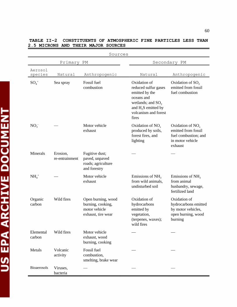
60

TABLE II-2 CONSTITUENTS OF ATMOSPHERIC FINE PARTICLES LESS THAN2.5 MICRONS AND THEIR MAJOR SOURCES

Sources

Primary PM Secondary PM

Aerosolspecies Natural Anthropogenic Natural Anthropogenic

SO Sea spray Fossil fuel Oxidation of Oxidation of SO4=

combustion reduced sulfur gases emitted from fossilemitted by the fuel combustionoceans andwetlands; and SO2

and H S emitted by2

volcanism and forestfires

2

NO — Motor vehicle Oxidation of NO Oxidation of NO3-

exhaust produced by soils, emitted from fossilx

forest fires, and fuel combustion; andlighting in motor vehicle

x

exhaust

Minerals Erosion, Fugitive dust; — —re-entrainment paved, unpaved

roads; agricultureand forestry

NH — Motor vehicle Emissions of NH Emissions of NH4+

exhaust from wild animals, from animal3

undisturbed soil husbandry, sewage,

3

fertilized land

Organic Wild fires Open burning, wood Oxidation of Oxidation ofcarbon burning, cooking, hydrocarbons hydrocarbons emitted

motor vehicle emitted by by motor vehicles,exhaust, tire wear vegetation, open burning, wood

(terpenes, waxes); burningwild fires

Elemental Wild fires Motor vehicle — —carbon exhaust, wood

burning, cooking

Metals Volcanic Fossil fuel — —activity combustion,

smelting, brake wear

Bioaerosols Viruses, — — —bacteria

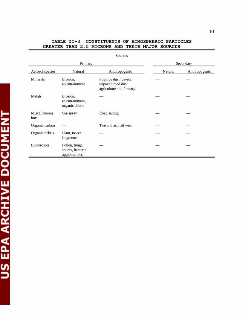
61

TABLE II-3 CONSTITUENTS OF ATMOSPHERIC PARTICLESGREATER THAN 2.5 MICRONS AND THEIR MAJOR SOURCES

Sources

Primary Secondary

Aerosol species Natural Anthropogenic Natural Anthropogenic

Minerals Erosion, Fugitive dust; paved, — —re-entrainment unpaved road dust,

agriculture and forestry

Metals Erosion, — — —re-entrainment,organic debris

Miscellaneous Sea spray Road salting — —ions

Organic carbon — Tire and asphalt wear — —

Organic debris Plant, insect — — —fragments

Bioaerosols Pollen, fungal — — —spores, bacterialagglomerates

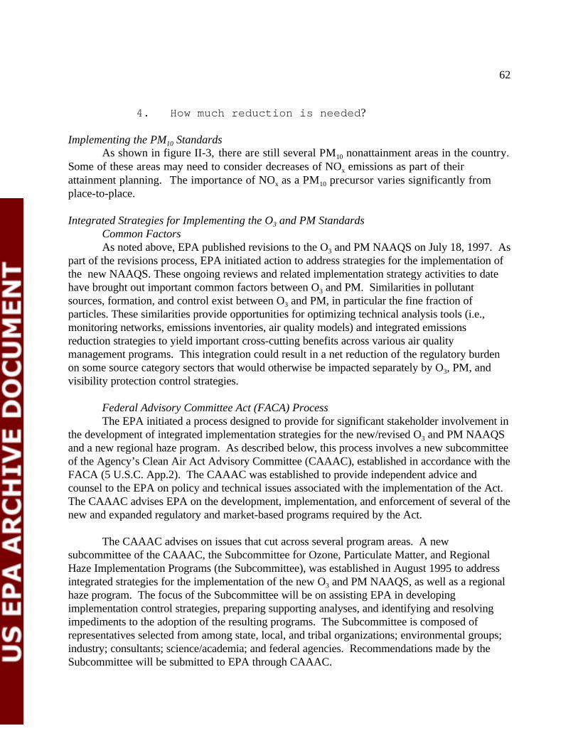
62

4. How much reduction is needed?

Implementing the PM Standards10

As shown in figure II-3, there are still several PM nonattainment areas in the country. 10

Some of these areas may need to consider decreases of NO emissions as part of theirx

attainment planning. The importance of NO as a PM precursor varies significantly fromx 10

place-to-place.

Integrated Strategies for Implementing the O and PM Standards3

Common FactorsAs noted above, EPA published revisions to the O and PM NAAQS on July 18, 1997. As3

part of the revisions process, EPA initiated action to address strategies for the implementation ofthe new NAAQS. These ongoing reviews and related implementation strategy activities to datehave brought out important common factors between O and PM. Similarities in pollutant3

sources, formation, and control exist between O and PM, in particular the fine fraction of3

particles. These similarities provide opportunities for optimizing technical analysis tools (i.e.,monitoring networks, emissions inventories, air quality models) and integrated emissionsreduction strategies to yield important cross-cutting benefits across various air qualitymanagement programs. This integration could result in a net reduction of the regulatory burdenon some source category sectors that would otherwise be impacted separately by O , PM, and3

visibility protection control strategies.

Federal Advisory Committee Act (FACA) ProcessThe EPA initiated a process designed to provide for significant stakeholder involvement in

the development of integrated implementation strategies for the new/revised O and PM NAAQS3

and a new regional haze program. As described below, this process involves a new subcommitteeof the Agency’s Clean Air Act Advisory Committee (CAAAC), established in accordance with theFACA (5 U.S.C. App.2). The CAAAC was established to provide independent advice andcounsel to the EPA on policy and technical issues associated with the implementation of the Act. The CAAAC advises EPA on the development, implementation, and enforcement of several of thenew and expanded regulatory and market-based programs required by the Act.

The CAAAC advises on issues that cut across several program areas. A newsubcommittee of the CAAAC, the Subcommittee for Ozone, Particulate Matter, and RegionalHaze Implementation Programs (the Subcommittee), was established in August 1995 to addressintegrated strategies for the implementation of the new O and PM NAAQS, as well as a regional3

haze program. The focus of the Subcommittee will be on assisting EPA in developingimplementation control strategies, preparing supporting analyses, and identifying and resolvingimpediments to the adoption of the resulting programs. The Subcommittee is composed ofrepresentatives selected from among state, local, and tribal organizations; environmental groups;industry; consultants; science/academia; and federal agencies. Recommendations made by theSubcommittee will be submitted to EPA through CAAAC.

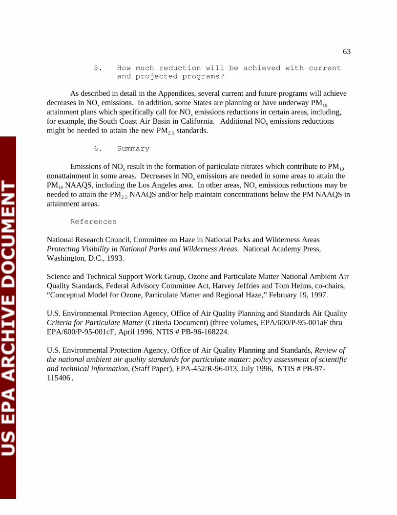
63

5. How much reduction will be achieved with currentand projected programs?

As described in detail in the Appendices, several current and future programs will achievedecreases in NO emissions. In addition, some States are planning or have underway PMx 10

attainment plans which specifically call for NO emissions reductions in certain areas, including,x

for example, the South Coast Air Basin in California. Additional NO emissions reductionsx

might be needed to attain the new PM standards.2.5

6. Summary

Emissions of NO result in the formation of particulate nitrates which contribute to PMx 10

nonattainment in some areas. Decreases in NO emissions are needed in some areas to attain thex

PM NAAQS, including the Los Angeles area. In other areas, NO emissions reductions may be10 x

needed to attain the PM NAAQS and/or help maintain concentrations below the PM NAAQS in2.5

attainment areas.

References

National Research Council, Committee on Haze in National Parks and Wilderness AreasProtecting Visibility in National Parks and Wilderness Areas. National Academy Press,Washington, D.C., 1993.

Science and Technical Support Work Group, Ozone and Particulate Matter National Ambient AirQuality Standards, Federal Advisory Committee Act, Harvey Jeffries and Tom Helms, co-chairs,“Conceptual Model for Ozone, Particulate Matter and Regional Haze,” February 19, 1997.

U.S. Environmental Protection Agency, Office of Air Quality Planning and Standards Air QualityCriteria for Particulate Matter (Criteria Document) (three volumes, EPA/600/P-95-001aF thruEPA/600/P-95-001cF, April 1996, NTIS # PB-96-168224.

U.S. Environmental Protection Agency, Office of Air Quality Planning and Standards, Review ofthe national ambient air quality standards for particulate matter: policy assessment of scientificand technical information, (Staff Paper), EPA-452/R-96-013, July 1996, NTIS # PB-97-115406.

64

E. Visibility Protection

1. Goals of the Program

Visibility is an air quality related value essential to the enjoyment of national parks,wilderness areas, and other scenic areas throughout our country. In section 169A of the 1977amendments to the CAA, Congress recognized that visibility was an important aspect of publicwelfare that should be protected. It established as a national goal “the prevention of any future,and the remedying of any existing, impairment of visibility in mandatory class I Federal areaswhich impairment results from man-made air pollution.” The CAA also calls for the developmentof programs to ensure reasonable progress toward the national goal, including theestablishment of a new regional haze program for the protection of visibility in mandatory FederalClass I areas across the country. These programs are to be implemented by the States and canbe regionally specific.

Regional haze and other visibility impairment is primarily caused by fine particles in the airwhich scatter or absorb light. These particles include, elemental carbon (soot), nitrates, organicmatter, soil dust, and sulfates. The major cause of visibility impairment in the Eastern UnitedStates is sulfate, formed primarily from SO emitted from coal combustion by electric utility2

boilers, while in the West the other four particle types play a greater role. Emissions of NO leadx

to the formation of particulate nitrates. Thus, the decreases in emissions of NO will help improvex

visibility and make progress toward the national goal.

2. Status of the Program

CAA Visibility RequirementsThe CAA includes two emissions control programs specifically concerned with visibility in

national parks and wilderness areas. One of these, the Prevention of Significant Deterioration program is directed mainly at new sources, as noted below. The other, a visibility protectionprogram, is aimed largely at existing sources.

Prevention of Significant Deterioration (PSD) The PSD program requires each new or expanded major emitting facility locating in a

clean air area to install the best available control technology and meet increments that limit thecumulative increases in pollution in clean air areas. Because all areas of the country are clean withrespect to the NO standard, the PSD program applies to major sources of NO throughout the2 x

nation.

The PSD program has protected visibility to some extent by decreasing the growth ofemissions of pollutants that contribute to regional haze, including SO and NO . The PSD2 x

65

Areas designated as mandatory class I areas are those national parks exceeding 6000 acres, wilderness areas10

and memorial parks exceeding 5000 areas, and all international parks which were in existence on August 7, 1977.

program includes a special air quality related values (AQRV) test for evaluating a major emittingfacility that might affect a Class I area. Many large national parks and wilderness areas aredesignated as Class I areas and therefore are subject to the most stringent increments. The federalland manager has the responsibility to protect the AQRV. The EPA’s PSD regulations are foundin the Code of Federal Regulations at 40 CFR 52.21.

Visibility RulesThe EPA issued visibility rules in 1980 (See 40 CFR 51.300-307 and 45 FR 80084)

requiring states containing mandatory class I areas to: (1) develop a program to assess andremedy visibility impairment from new and existing sources; (2) develop a long-term strategy toassure progress toward the national goal; (3) develop a visibility monitoring strategy; (4) consider“integral vistas” outside of class I areas in all aspects of visibility protection; and (5) notify Federalland managers (FLM) of proposed new major stationary sources and consider visibility analysesconducted by FLMs in their permitting decisions (40 CFR 51 subpart P). These visibility rules layout a process for visibility impacts from a single source or small group of sources which mayreasonably be anticipated to cause or contribute to visibility impairment in a Federal Class I area. The process is initiated by a certification of impairment by a FLM. The State determines whetherthe impairment is attributable to the source(s) and, if so, requires controls to reduce impairment.

The 1980 visibility regulations required 36 States containing mandatory Class I areas tosubmit strategies for monitoring visibility. The EPA completed in 1985 Federal regulations toestablish a national visibility monitoring network which would be cooperatively managed by EPA,Federal land management agencies, and State air agency representatives. This network is nowknown as IMPROVE (Interagency Monitoring of Protected Visual Environments). Due toresource limitations, IMPROVE monitors could not be placed in all 156 mandatory class I areas.Instead, the IMPROVE Steering Committee has selected a set of priority sites. Data are currentlybeing collected at more than 40 Class I locations. The IMPROVE monitoring protocol specifiesaerosol, photographic, and optical (light extinction) measurements twice a week.

At that time of the rulemaking, EPA also expressed its intention to regulate regional hazeat some future date when monitoring techniques are improved and the relationship between airpollutants and visibility impairment is better established. Much progress has been made intechnical areas important to the successful implementation of a regional haze program,including areas such as visibility monitoring, regional scale modeling, and scientificknowledge of the regional effects of particles on visibility. As described below, EPA plans tobegin a new regional haze program for the protection of visibility in mandatory Federal Class Iareas across the country.10

Grand Canyon Visibility Transport Commission Section 169B of the 1990 CAA amendments required the establishment of the Grand

66

The Commission consists of the Governors, or their designees, from the States of Arizona, California, Colorado,11

Nevada, New Mexico, Oregon, Utah, and Wyoming; the President of the Navajo Nation; the Chairman of the Hopi Tribe;the Governor of the Pueblo of Acoma; the Chairman of the Hualapai Tribe; and ex-officio members from EPA, Bureau ofLand Management, National Park Service, United States Forest Service, United States Fish and Wildlife Service, and theColumbia River Inter-Tribal Fish Commission.

Canyon Visibility Transport Commission (GCVTC ). The Commission was charged with11

assessing adverse impacts on visibility from projected growth in the region, and requires theCommission to recommend measures to EPA for addressing adverse impacts to visibility in theregion. The Commission formally adopted its report to the EPA on June 10, 1996. The EPA isto use the Commission’s recommendations as guidance for developing national strategies and/orrulemaking. Implementation of specific program components will be the responsibility of tribes,states, and, in some cases, federal agencies. The primary recommendations in the Commission’sreport include: air pollution prevention measures such as energy conservation and increasedenergy efficiency; tracking of emissions growth in clean air corridors; development of a plan foran emissions cap and trading program for stationary sources; and establishing a regional emissionsbudget for mobile sources.

Regional Haze RulesThe Administrator of EPA signed the notice of proposed rulemaking for the regional

haze rules on July 18, 1997. These rules are a continuation of the 1980 rules. From the timethe GCVTC report is received, section 169B requires EPA to issue rules within 18 months toassure reasonable progress toward remedying adverse impacts due to regional haze. Afterestablishment of a regional haze program, States affected by these rules are required, undersection 169B(e)(1), to revise their state implementation plans (SIPs) within 12 months to includesuch emission limits, schedules of compliance, and other measures as may be necessary forprogram implementation. Relation to NO NAAQS Review2

As described in the final rulemaking notice of October 8, 1996 (61 FR 52852) on revisionto the NO NAAQS, EPA determined that establishment of a secondary NO standard to protect2 2

visibility is not appropriate. While NO can contribute to brown haze, there is no established2

relationship between ground level NO concentrations at a given point and visibility impairment2

due to a plume or regional haze. Furthermore, regional scale NO light extinction is much less2

than aerosol extinction. These considerations helped lead to the conclusion that establishment ofa secondary NO standard to protect visibility would not be appropriate. 2

Relation to PM Standard ReviewIn reviewing the NAAQS for PM, EPA also considered the appropriateness of a

secondary standard to address a number of welfare effects, specifically including visibility. Because of regional variations in visibility conditions created by background concentrations offine particles, annual average humidity, pollutant mix, and resulting total light extinction,however, a regional haze program under the regulatory authority in section 169A may bepreferable to setting a secondary NAAQS. As described in the July 18, 1997 Federal Register,

67

EPA set the secondary PM standards identical to the primary standards which, in conjunctionwith a regional haze program under sections 169A and 169B of the Act, EPA believes is the mostappropriate and effective means of addressing the welfare effects associated with visibilityimpairment. Together, the two programs and associated control strategies should provideappropriate protection against the effects of PM on visibility and allow all regions of the countryto make reasonable progress toward the national visibility goal.

3. Science of NO and Visibilityx

Visibility Basics For an object to be seen against a background, there must be sufficient contrast between

the object and its background. That is, the light from the object and the background must besufficiently different in apparent brightness or color to make the object stand out against thebackground. Light from objects and their background viewed through the atmosphere from adistance are modified by the particles and gases in the atmosphere (primarily clean air).

Light as it traverses the atmosphere is scattered (i.e., redirected in directions) andabsorbed (i.e., converted from light to heat) by the particles and gases in the atmosphere. Thisaffects the appearance of scenes in two ways. The image-forming light from scenic features isdiminished since a fraction of the light is scattered or absorbed; non-image-forming light isscattered into the sight path. Both of these effects lower the contrast between object andbackground, and cause the scene to be more obscured. This decrease in contrast is furtherdecreased with distance to the scenic feature being viewed, and with increased concentration ofairborne particles.

Many studies have been published on visibility conditions and related aerosolconcentrations. The NAPAP report (1991) lists 33 aerosol and visibility databases. From thesestudies, the major contributors to visibility impairment from natural and man-made sources aresulfate particles, organic particles, elemental carbon, suspended dust, and nitrate particles.

Regional haze is primarily caused by fine particles in the air, typically less than 2.5 micronsin diameter, which scatter and absorb light. These particles include sulfates, nitrates, organicmatter, elemental carbon (soot), and soil dust (NRC, 1993). The fate of regional haze is afunction of meteorological and chemical processes, sometimes causing fine particle loadings toremain suspended in the atmosphere for long periods of time (3-5 days) and to be transportedlong distances (thousands of kilometers) from their sources. A large fraction of anthropogenicairborne particles (sulfates, nitrates, and some organic particles) accumulates in the 0.1-1.0micron diameter range. These particles can survive in the atmosphere for several days and canbe transported hundreds or even thousands of kilometers from their sources to remotelocations, such as national parks and wilderness areas (NRC, 1993). During transport, theemissions from many different sources can become mixed, making it difficult to assess theeffects of individual sources on visibility. Types of Visibility Impairment

68

Visibility effects are manifested in two principal ways: (1) as local impairment (e.g.,plumes and localized hazes) and (2) as regional haze. Local-scale impairment is defined asimpairment that is "reasonably attributable" to a single source or group of sources. Visibilityimpairment in some urban areas can be dominated by local rather than regional sources,particularly in mountain valleys in the winter and in meteorologically stagnant conditions.

The second category of impairment, regional haze, is produced from a multitude ofsources combined over many days. Regional haze impairs visibility in every direction over alarge area. Objects on the horizon are obscured and the texture of nearby objects is reduced. In some cases, the haze may be elevated and appear as layers of discoloration.

The contribution by particles from both natural and man-made sources are highly variable. Natural particle sources such as wildfires, windblown dust, salts from ocean spray, etc. are highlyvariable across time and space with the result that natural background levels of visibility are highlyvariable. Concentrations of man-made and natural particles also vary because of the influence ofvariable meteorology responsible for atmospheric transport and dispersion. (For furtherinformation on visibility, see the 1979 Report and the 1990 NAPAP Report "Acidic Deposition: State of Science and Technology, Volume III, Report Number 24.)

Visibility MetricsVisual range, which is defined as the greatest distance that a large dark object can be seen

against the background sky, is the oldest and most commonly used visibility metric. Visual rangewas developed and continues to function well as an aid in military operations and transportationsafety. Airport observations of visual range have been made since 1919, and have been computerarchived since the late 1940's. Daylight observations involve viewing preselected visibilitymarkers (large dark objects) at known distances from the observation point to determine the mostdistant marker that is visible.

Another traditional visibility metric is extinction coefficient, which is the attenuation oflight per unit distance due to scattering and absorption by gases and particle in the atmosphere. Extinction coefficient is expressed in inverse length units (e.g., km ) and is used primarily by-1

scientists studying the causes of reduced visibility. Direct relationships exist betweenconcentrations of atmospheric constituents and their contribution to extinction coefficient. Apportioning extinction coefficient to atmospheric constituents provides a method to estimatechange in visibility caused by change in constituent concentrations. Calculation of the extinctioncoefficients from air quality models can be used to estimate the expected visibility changes fromemission changes.

Visibility Impairing ParticlesLight scattering, and to a lesser degree, light absorption by suspended particles are the

most important contributors to visibility degradation. The influence of particles depends on theconcentration, composition, and the size of the particles. Particles composed of materials such as

69

sulfates and nitrates absorb under high relative humidity conditions. Since the solution drops arelarger than the dry particles, visibility impairment by sulfate and nitrate particles increases duringhigh humidity conditions.

Sulfate, nitrate, and organic carbon are major contributors to visibility degradation. Theseparticles begin as gaseous emissions and undergo chemical transformation in the atmosphere. These particles are mostly in a size range from about 0.1 to 1.0 microns diameter which scattersmore light for the same mass concentration than smaller or larger particles. That is, the particlesthat scatter light most efficiently per unit mass are those of approximately the same size aswavelengths of visible light (0.4-0.7 microns). Coarse particles (i.e., those in the 2.5 to 10micron size range) also impair visibility, although less efficiently than fine particles. Blackcarbon, primarily from incomplete combustion such as in diesel exhaust or wood smoke, is theprincipal cause of light absorption in the atmosphere. Sulfates and nitrates readily absorb waterfrom the atmosphere and grow in size in a nonlinear fashion as relative humidity levelsincrease. Because humidity varies seasonally, the visibility impacts of the sulfate and nitrateparticles also varies by season.

NO Emissionsx

As described in the “Ozone” section of this document, NO is formed during combustion orany high temperature process involving air. The NO is converted to NO by O or other2 3

atmospheric oxidants. The NO then participates in various reactions to form other substances,2

including O and PM.3

Nitrate ParticulatesNitrate airborne particles can be produced by several mechanisms. One major mechanism

of nitrate formation involves the gas-phase reaction of NO with OH to produce nitric acid,2

HNO . The gaseous nitric acid can react at airborne particle surfaces to form nitrate salts. For3

example, a particle containing calcium carbonate can neutralize the nitric acid to produce calciumnitrate; it follows that nitrate size distributions depend, in part, on the size distributions ofparticles on which they react (NRC, 1993). Ammonia gas (NH ) is important in the generation of3

sulfate and nitrate particles through the neutralization of sulfuric and nitric acid. Whenconcentrations of NH and HNO are sufficiently high, ammonium nitrate (NH NO ) can be3 3 4 3

formed. Ammonium nitrate is often found in submicron particles in locations such as Denver orLos Angeles. However, little submicron ammonium nitrate is typically found in parts of the nationwhere ammonia concentrations are low and acid sulfate concentrations are high (NRC, 1993). (See additional discussion in the “Particulate Matter, Emissions Sources and Formation Processesof Particles” section of this document.)

NO2

The only gas that absorbs visible light to any appreciable extent at concentrations expectedin the atmosphere is NO . NO is a strong absorber of visible and ultraviolet light and can thereby2 2

contribute to haze. In addition, NO has a broad absorption band at the blue end of the spectrum;2

70

consequently, when NO concentrations are high, the atmosphere has a distinct brownish color. 2

However, because of its high reactivity and relatively short lifetime, NO does not normally2

contribute significantly to haze in remote areas; it is a problem only in areas close to sources(NRC, 1993).

The most significant optical effect of NO involves discoloration (EPA, 1996). NO2 2

appears as a yellow to reddish-brown gas because it strongly absorbs blue light, allowing redwavelengths to reach the eye. The extent to which NO filters out blue light is determined by the2

integral of NO concentration along the sight path. In regard to regional haze, because the effect2

of NO depends on the product of the pollution concentration and the viewing path length, the2

coloration of 0.05 ppm NO over 10 km is the same as 0.5 ppm over 1 km. When NO is2 2

dispersed over a large area, as in the case of urban emissions, ground level concentrations atindividual points may be less than a national standard but because an observer views the entireNO mass, the urban plume appears of brownish color.2

Significance of Anthropogenic Sources of Fine ParticlesThe concentrations of background fine particles are generally small when compared

with concentrations of fine particles from anthropogenic sources. The same relationship holdstrue when one compares light extinction due to background fine particles with light extinctiondue to anthropogenic fine particles. Anthropogenic contributions account for about one-thirdof the average extinction coefficient in the rural West and more than 80 percent in the ruralEast (NAPAP, 1991). In the eastern United States, sulfates dominate fine particleconcentrations, stemming from regional SO emissions. In contrast, nitrate plays a small role2

in the East but is significant in areas of the West; for example, nitrates dominate the overalllight extinction in the mountainous areas just outside Los Angeles, with most of the nitrateformation in this area coming from NO emissions within the urban area (EPA, 1996).x

Monitoring DataWhile the amount of total light extinction varies significantly across the country, so

does the mix of visibility-impairing pollutants from region to region. As described in Table II-4, IMPROVE monitoring data were used to establish annual apportionment of current aerosolcomponents to the total visibility impairment for class I areas. This gives an indication of therelative contribution to visibility impairment due to nitrates in a variety of areas. Nitrates arethe largest contributor to light extinction in National Parks and Wilderness Areas in SouthernCalifornia.

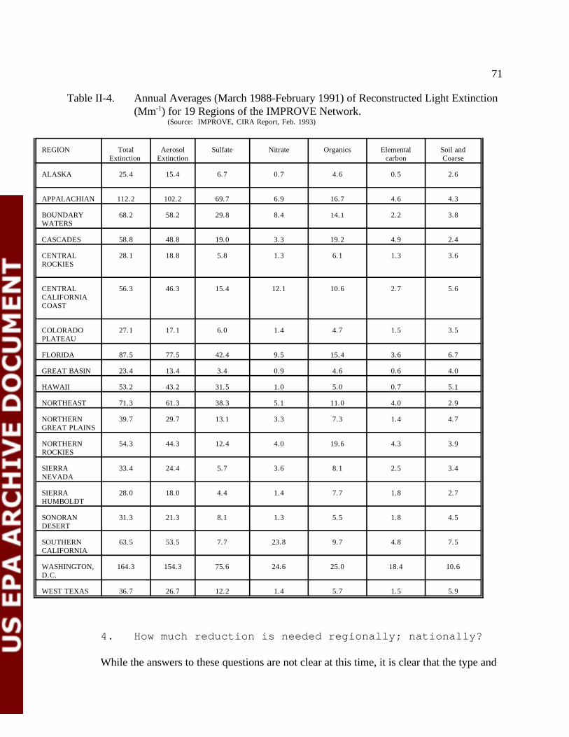
71

Table II-4. Annual Averages (March 1988-February 1991) of Reconstructed Light Extinction(Mm ) for 19 Regions of the IMPROVE Network.-1

(Source: IMPROVE, CIRA Report, Feb. 1993)

REGION Total Aerosol Sulfate Nitrate Organics Elemental Soil andExtinction Extinction carbon Coarse

ALASKA 25.4 15.4 6.7 0.7 4.6 0.5 2.6

APPALACHIAN 112.2 102.2 69.7 6.9 16.7 4.6 4.3

BOUNDARY 68.2 58.2 29.8 8.4 14.1 2.2 3.8WATERS

CASCADES 58.8 48.8 19.0 3.3 19.2 4.9 2.4

CENTRAL 28.1 18.8 5.8 1.3 6.1 1.3 3.6ROCKIES

CENTRAL 56.3 46.3 15.4 12.1 10.6 2.7 5.6CALIFORNIACOAST

COLORADO 27.1 17.1 6.0 1.4 4.7 1.5 3.5PLATEAU

FLORIDA 87.5 77.5 42.4 9.5 15.4 3.6 6.7

GREAT BASIN 23.4 13.4 3.4 0.9 4.6 0.6 4.0

HAWAII 53.2 43.2 31.5 1.0 5.0 0.7 5.1

NORTHEAST 71.3 61.3 38.3 5.1 11.0 4.0 2.9

NORTHERN 39.7 29.7 13.1 3.3 7.3 1.4 4.7GREAT PLAINS

NORTHERN 54.3 44.3 12.4 4.0 19.6 4.3 3.9ROCKIES

SIERRA 33.4 24.4 5.7 3.6 8.1 2.5 3.4NEVADA

SIERRA 28.0 18.0 4.4 1.4 7.7 1.8 2.7HUMBOLDT

SONORAN 31.3 21.3 8.1 1.3 5.5 1.8 4.5DESERT

SOUTHERN 63.5 53.5 7.7 23.8 9.7 4.8 7.5CALIFORNIA

WASHINGTON, 164.3 154.3 75.6 24.6 25.0 18.4 10.6D.C.

WEST TEXAS 36.7 26.7 12.2 1.4 5.7 1.5 5.9

4. How much reduction is needed regionally; nationally?

While the answers to these questions are not clear at this time, it is clear that the type and

72

amount of emissions reductions needed varies from area to area. Visibility conditions varyregionally, as a function of background concentrations of fine particles, average relative humiditylevels, and anthropogenic particle loadings, all of which are generally higher in the East than in theWest. It is important to note that even in areas with relatively low concentrations ofanthropogenic fine particles, such as the Colorado plateau, small increases in emissions can lead tosignificant decreases in visual range. This is one reason for the emphasis on protecting visual airquality in the highly valued national parks and wilderness areas in the Colorado plateau region. Inareas with relatively higher fine particle concentrations, such as the Great Smoky MountainsNational Park, it takes a greater reduction in ambient concentration to make an equivalentimprovement in visual range.

Most visibility impairment in national parks and wilderness areas results from thetransport by winds of emissions and secondary airborne particles over great distances (typicallyhundreds of kilometers). Consequently, visibility impairment is usually a regional problem, not alocal one. Progress towards the national goal of remedying and preventing anthropogenicvisibility impairment in Class I areas will require regional programs that operate over largegeographic areas; strategies should be adopted that consider many sources simultaneously on aregional basis (NRC 1993). The outcome of the GCVTC report and EPA’s subsequentrulemaking will help define the needed reductions to meet the national goals.

5. How much reduction will be achieved with current andprojected programs?

Implementation of the CAA will achieve substantial decreases in NO emissions. The PSDx

program has managed atmospheric loadings from new sources and has safeguarded some largeparklands from excessive emissions from new sources. Programs that may achieve additional NOx

emissions reductions are described in the Appendices to this document. Further, the revisions tothe PM and O NAAQS could lead to additional emissions reductions.3

6. Summary

Visibility impairment can occur due to local plumes or widespread regional haze. Thesources of locally visible plumes are easy to identify, for example, the smoke from a power plantstack or from a burning field. However, when plumes are carried by winds, they become morediffuse, and the sources are identified less readily. In regions with many sources, the plumes canmerge and become mixed with the emissions from many sources, such as motor vehicles, powerplants, and industrial operations. The result is a widespread haze in which individual contributionsfrom the various sources are virtually indistinguishable.

In most cases, visibility degradation is caused by five kinds of particulate substances:sulfates, nitrates, organic matter, elemental carbon, and soil dust. Regional haze is producedfrom a multitude of sources and impairs visibility in every direction over a large area, such asan urban area, or possibly over several states. Multiple sources may combine over many daysto produce haze, which is often regional in scale. The fate of regional haze is a function of

73

meteorological and chemical processes, sometimes causing fine particle loadings to remainsuspended in the atmosphere for long periods of time and to be transported long distancesfrom their sources. The major cause of visibility impairment in the East is sulfate, formedprimarily from SO emitted from coal combustion by electric utility boilers, while in the West the2

other four particle types play a greater role. Emissions of NO lead to the formation of particulatex

nitrates; thus, the reduction in emissions of NO will help improve visibility and make progressx

toward the national goal.

References

Grand Canyon Visibility Transport Commission, Recommendations for Improving WesternVistas, June 10, 1996 report of the Grand CanyonVisibility Transport Commission to the UnitedStates Environmental Protection Agency, June 10, 1996.

National Acid Precipitation Assessment Program (NAPAP) 1979 and the 1990 Reports AcidicDeposition: State of Science and Technology, Volume III, Report Number 24, entitled“Visibility: Existing and Historical Conditions - Causes and Effects.”

National Acid Precipitation Assessment Program (NAPAP), (1991). Office of the Director,Acid Deposition: State of Science and Technology. Report 24, “Visibility: Existing andHistorical Conditions - Causes and Effects.” Washington, D.C.

National Research Council, Committee on Haze in National Parks and Wilderness AreasProtecting Visibility in National Parks and Wilderness Areas. National Academy Press,Washington, D.C., 1993.

Science and Technical Support Work Group, Ozone and Particulate Matter National Ambient AirQuality Standards, Federal Advisory Committee Act, Harvey Jeffries and Tom Helms, co-chairs,“Conceptual Model for Ozone, Particulate Matter and Regional Haze,” February 19, 1997.

U.S. Environmental Protection Agency, Office of Air Quality Planning and Standards,Effects of the 1990 Clean Air Act Amendments on Visibility in Class I Areas: An EPA Report toCongress. Research Triangle Park, N.C., 1993.

U.S. Environmental Protection Agency, Office of Air Quality Planning and Standards, Review ofthe national ambient air quality standards for particulate matter: policy assessment of scientificand technical information, (Staff Paper), EPA-452/R-96-013, July 1996, NTIS # PB-97-115406.

74

III. Additional Public Health and Environmental Impacts from NOx

Emissions

A. Drinking Water

As described in the section on “Acid Deposition,” nitrate and nitrite leaching aggravatesthe effects of acidification, both long term (e.g. cation leaching) and episodically (e.g. Al peaks). Adding inorganic N to freshwater ecosystems can eutrophy as well as acidify the waters whenthey are already rich in phosphorus or, more rarely, when N is the limiting nutrient (Vitousek etal, 1997:10; Church, 1997:17).

Most freshwater ecosystems will not be eutrophied by additional nitrate or nitrite leachingbecause phosphorous is the limiting nutrient. (Because the direct contribution of nitrite istypically very small compared to nitrate, sometimes this process is called simply “nitrateleaching.”) Nitrate leaching has implications that go beyond its eutrophying and acidifyingeffects. Because primary producers (plants) in most freshwater systems do not assimilate addednitrate, this ion can remain in the water and be transported long distances downstream. Bycontrast, acidity may be neutralized by natural processes before it reaches large streams, lakes orestuaries. This characteristic leads to two impacts that can occur downstream: elevated levels ofnitrate in drinking water supplies (discussed below) and eutrophication of estuaries and coastalwaters (discussed in the following section). These downstream impacts can occur in hydrologicalsystems even where acidification is not a problem.

Under the Safe Drinking Water Act, EPA has set maximum contaminant levels (MCLs)for nitrate and nitrite in drinking water to protect human health. These levels are established at 10milligrams per liter (mg/L) of nitrate N and 1 mg/L of nitrite N (40 CFR 141.62). The primaryadverse human health effect associated with exposure to nitrate or nitrite is methemoglobinemia(National Research Council, 1995:2). To cause methemoglobinemia, nitrate must be convertedinto nitrite. Methemoglobinemia occurs when nitrite oxidizes iron (Fe ) in blood into FE , a2+ 3+

form that does not allow oxygen transport, and can cause brain damage or death (Vitousek et al,1997:9). This condition in adults is rare (National Research Council, 1995:2), but is a significantconcern for infants because microbes in an infant’s stomach may convert high levels of nitrate tonitrite (Vitousek et al, 1997:9). Insufficient oxygenation of the blood is characterized by bluishskin and lips (“blue baby syndrome”). The National Research Council concluded, in 1995, that“results from epidemiological studies are inadequate to support an association between nitrate ornitrite exposure from drinking water in the United States and increased cancer rates in humans”(National Research Council, 1995:2). However, an epidemiological study, published in 1996, ofrural populations using community water supplies in Nebraska, concluded that “long-termexposure to elevated nitrate levels in drinking water may contribute to the risk for Non-Hodgkin’s

75

Lymphoma (NHL)” (Ward et al, 1996:465).

The contribution of atmospheric N deposition to elevated levels of nitrate in drinkingwater supplies is an evolving impact area. The Ecological Society of America (ESA) has includeddiscussion of this impact in a recent major review of causes and consequences of human alterationof the global N cycle in its Issues in Ecology series (Vitousek et al, 1997:9). This series isdesigned to report, in language understandable by non-scientists, the consensus of a panel ofscientific experts on issues relevant to the environment. Issues in Ecology is supported by thePew Scholars in Conservation Biology Program and ESA, a national professional society foundedin 1915.

For decades, N concentrations in major rivers and drinking water supplies have beenmonitored in the United States, Europe, and other developed regions of the world. Monitoringdata from public water systems in the United States show that surface water sources of drinkingwater do not exceed MCLs for nitrate and nitrite, with very rare exceptions unrelated to airbornedeposition. On the other hand, analysis of these data confirms a substantial rise of N levels insurface waters, which are highly correlated with human-generated inputs of N to their watersheds. These N inputs are dominated by fertilizers and atmospheric deposition (Vitousek et al, 1997:9). Nitrate levels in the Mississippi River have more than doubled since 1965; they have risen inmajor rivers of the northeastern U.S. by three- to ten-fold since 1900 (Vitousek et al, 1997:9).

Agricultural sources dominate human-generated inputs of N in regions with intensivefarming, including the Mississippi River basin and Texas. In other areas, such as the northeasternUnited States, NO emissions from industrial origin are the major factor in river export of N tox

lakes, major rivers, and estuaries (Howarth et al, 1996). Relatively low nitrate water fromforested watersheds can serve to dilute higher nitrate water from urban or agricultural watershedsfor many towns and cities. As water from forested watersheds increases in nitrate, therefore, itsdilution capability diminishes and thus can threaten community water supplies even before actualnitrate concentrations exceed the drinking water standard (Ryan, 1996). Nitrate levels tend to behigher in private wells than community water supplies due to lack of regular testing, simplerconstruction, and shallow depth (Ward et al, 1996:165). High levels of nitrate in private wellwater typically indicate that pollution is seeping in from septic tanks, animal wastes, fertilizers,municipal landfills, or other nonpoint sources (EPA, 1996).

Increases in atmospheric N deposition to sensitive forested watersheds approaching Nsaturation would be expected to result in increased nitrate concentrations in stream water. Onlyone incidence of this phenomenon in the United States has been documented in peer-reviewedliterature, although it has been well-established for areas in Germany and the Netherlands (Rigganet al, 1985:786). High nitrate concentrations from chaparral watersheds have been found instream water in the South Coast (Los Angeles County, CA) Air Basin (Riggan et al, 1985, 1994). Stream water nitrate concentrations in watersheds subject to chronic air pollution were two tothree orders of magnitude greater than in chaparral regions outside the air basin. Within the SanGabriel Mountains, nitrate concentrations were greatest, as high as 7.0 mg/L, where watersheds

76

adjoin the urbanized basin and may contribute to existing groundwater nitrate pollution (Riggan etal, 1985:786, 781).

Some high nitrate concentrations reported in this study were measured after a stormwashed ash from burned landscape into the stream water. Wildfires in chaparral subject tochronic air pollution may cause inordinately high stream water nitrate loading which, whenreleased through high stream discharge and channel scouring, could saturate the aquatic systemand seriously pollute downstream waters (Riggan et al, 1985:788). These chaparral watershedsare specialized ecosystems and probably are not typical of United States watersheds in general. Nonetheless, high nitrate concentrations have also been observed in forest soils in the vicinity ofthe Asheville Watershed in western North Carolina; the amounts in soil solution suggest elevatedlevels of nitrate in groundwater (Smithson, 1997).

While observational evidence directly linking atmospheric deposition to elevated levels ofnitrate in drinking water supplies is very limited, atmospheric deposition can supply N toecosystems in a manner not dissimilar to fertilizer application (Vitousek et al, 1996:7-8). In fact,researchers have noted that some amount of atmospheric N deposition can be beneficial toagriculture, as fertilizer, in some areas, depending on the soil, crops harvested, biological uptakeprocesses, and other factors (Acid Rain Program, 1995:36). Thus, one would expect thatdecreases in atmospheric N deposition to N-sensitive watersheds resulting from decreases in localor transported NO or ammonia N emissions would lessen the contribution of airborne depositionx

to elevated levels of nitrate in drinking water supplies.

References

Acid Rain Program. 1995. Adverse Effects of Nitrogen Oxides (NO ) and Benefits of Reduction,x

draft staff assessment paper (Air Docket A-95-28, Item II-A-13). U. S. Environmental ProtectionAgency; Washington, DC. December. Devesa, S.S. and T. Fears. 1992. “Non-Hodgkin’s Lymphoma Time Trends: United States andInternational Data” Cancer Res. 1992; 52(suppl): 5432S-5449S.

Howarth, R.W., G.Billen, D.Swanwy, A. Townsend, N. Jaworski, K. Lajtha, J.A.Downing,R.Elmgren, N. Caraco, T. Joddan, F. Berendse, J. Freney, V. Kudeyarov, P. Murdoch, ZhuZhao-Liang. 1996. “Regional nitrogen budgets and riverine N &P fluxes for the drainages to theNorth Atlantic Ocean: Natural and human influences.” Biogeochemistry (in press).

National Research Council. 1995. Nitrate and Nitrite in Drinking Water. Washington, DC:National Academy Press.

Riggan, P.J., R.N. Lockwood, and E.N. Lopez, “Deposition and Processing of Airborne NitrogenPollutants in Mediterranean-Type Ecosystems of Southern California” Environmental Scienceand Technology, vol. 19 (p. 781-789), 1985.

77

Riggan, P.J., R.N. Lockwood, P.M.Jacks, C.G.Colver,F.Weirich, L.F.DeBano, and J.A.Brass,“Effects of Fire Severity on Nitrate Mobilization in Watersheds Subject to Chronic AtmosphericDeposition” Environmental Science and Technology, vol. 28 (p. 369-375), 1994.

Ryan, Douglas F., USDA, Forest Service, Forest Environment Research, personal communicationNovember 7, 1996.

Smithson, Paul. 1997. Unpublished doctoral dissertation, North Carolina State University,Department of Soil Science (p. 95-96, 115, 122, 130), 1997.

U.S. Environmental Protection Agency, “Environmental Indicators of Water Quality in the UnitedStates: Fact Sheets”. EPA-841-F-96-001, 1996.

Vitousek, Peter M., John Aber, Robert W. Howarth, Gene E. Likens, et al. 1997. HumanAlteration of the Global Nitrogen Cycle: Causes and Consequences. Issues in Ecology. Published by Ecological Society of America, Number 1, Spring 1997.

Ward, M.H., S.D. Mark, K.P. Cantor, D. D. Weisenburger, A. Correa-Villasenor, and S.H.Zahm. 1996. “Drinking Water Nitrate and the Risk of Non-Hodgkin’s Lymphoma”Epidemiology 7:465-471.

78

B. Eutrophication

1. Goals of the Program

Eutrophication has been identified as the most serious pollution problem facing theestuarine waters of the United States (NRC, 1993). In fact, 54 percent of impacted square milesof estuaries that have been assessed have been shown to be impaired by nutrients (EPA 1994). N is the limiting nutrient controlling eutrophication in most temperate estuaries (Nixon, 1986,Swain et al, 1994) and some limited percentage of freshwater lakes (EPA, 1993). Studies of Nloadings to estuarine and coastal systems within the United States and worldwide have shownthat N deposited from the atmosphere is a significant portion of the total N loadings, rangingfrom 10 to 70 percent, with 27 percent of the N loadings delivered to the Chesapeake Bayoriginating from atmospheric sources (Linker et al, 1993; Paerl. 1993, Valigura et al, 1995). Nhas been shown to be the nutrient controlling the baywide reductions of bottom water dissolvedoxygen in Chesapeake Bay (Thomann et al. 1994).

The EPA Office of Air Quality Planning and Standards’ program addressing the issue ofN deposition and resultant eutrophication impacts is the Great Waters Program. The charge ofthe Great Waters program, under section 112(m) of the CAA amendments, is to evaluate thedeposition of hazardous air pollutants (and other pollutants at the discretion of theAdministrator) to the Great Lakes, Lake Champlain, Chesapeake Bay and other estuarine andcoastal waters. Given the discretion for additional pollutants, and the lack of attention to theNO /eutrophication link, EPA chose to use this program as a vehicle to address this Nx

deposition/eutrophication issue. The Great Waters Program provides information in biennialreports to Congress regarding: the adverse effects of the deposition on human health and theenvironment; the proportion of the loading which comes from the atmosphere; the sources of thepollution; evaluations of the effectiveness of existing regulatory programs in addressing theseproblems; and, ultimately, what changes to regulations are needed to prevent the identifiedadverse effects. The overall goal of the Great Waters Program is to identify and prevent adverseeffects due to air pollutants deposited to aquatic ecosystems.

The Great Waters program works cooperatively with a number of other EPA offices, theNational Oceanic and Atmospheric Administration (NOAA), and state agencies with respect tothe N deposition/eutrophication issue, including the Chesapeake Bay Program Office, the Officeof Water, various National Estuary Programs (e.g., Tampa Bay), and NOAA’s Air ResourcesLaboratory and Coastal Ocean Program Office. The goals of these programs are complementaryto and intersect with the Great Waters goal of characterizing and addressing the water qualityproblems due to atmospheric deposition of N compounds.

2. Status of the Program

79

Great Waters ProgramBecause of established monitoring data bases, monitoring methodology research,

enhanced monitoring networks, and linked airshed-watershed-water quality models available orunder development, the Great Waters Program has been focused on further advancing efforts inspecific geographic areas. For estuarine issues, that work has focused on the Chesapeake Bay. Participants in the Great Waters Program believe that providing a comprehensive evaluation in awell-studied geographic area provides an invaluable understanding of the total scope of theproblem, causes, processes, and the range of feasible control/reduction/prevention managementoptions -- an understanding that would be impossible to develop with a number of disparate,less-intensive studies. The Great Waters Program has already found that the informationdeveloped through the Chesapeake Bay Program is directly applicable to other east coastestuarine systems with adjustments needed for the respective waterbody's watershedcharacteristics. This direct transferability of technologies and technical findings will savesimilar financial investments and years of effort by the many other place-based estuarine andcoastal management programs along the Atlantic and Gulf coastlines.

Since the First Report to Congress on the atmospheric deposition of pollutants to theGreat Waters, studies of other coastal waters, at National Estuary Program waters in particular,have investigated the significance of atmospheric deposition of N compounds to their waters. Toimprove understanding and reduction of N deposition to Chesapeake Bay and other coastalwaters, the Chesapeake Bay Program, various National Estuary Programs, and the Gulf ofMexico Program continue to develop and refine modeling and monitoring efforts by addressinguncertainties such as N retention in watersheds, the differences in transport and fate of various Ncompounds, and the contribution of near shore ocean waters to the N inputs to estuaries.

The second report to Congress on the atmospheric deposition of pollutants to the GreatWaters was completed in June 1997 (EPA, 1997). The report continues to find N compounds apollutant of concern. Atmospheric deposition of N compounds can contribute significantly toeutrophication in coastal waters, where plant productivity is usually limited by N availability.Accelerated eutrophication and its subsequent effects such as nuisance algal blooms and reducedoxygen levels pose significant problems for Chesapeake Bay and many other estuaries. Thereport also indicates that substantial progress has been made in addressing N contamination issuesin Chesapeake Bay, the largest United States estuary. A strategy has been developed by theChesapeake Bay Program for reducing the N load to the Bay. Part of this process includes thelarge-scale modeling and understanding of the type and geographic origin of airborne N to theBay. Significant data also have been collected on rates and amounts of N deposition (includingcomparison of direct and indirect deposition and of wet and dry deposition), and models havebeen developed to evaluate the impact of several N reduction scenarios on the Bay's water quality.

Chesapeake Bay ProgramThe Chesapeake Bay, largest of the 130 estuaries in the United States, was the first in the

nation to be targeted for restoration as an integrated watershed, airshed, and ecosystem. The64,000 square mile drainage basin covers parts of six states including New York, Pennsylvania,Maryland, Delaware, West Virginia, and Virginia and includes more than 150 tributaries. Now

80

in its thirteenth year, the Chesapeake Bay Program is a unique, regional, federal-state-localpartnership that has directed and coordinated Chesapeake Bay restoration since the signing of thehistoric 1983 Chesapeake Bay Agreement. The Chesapeake Bay Program includes the state ofMaryland, the Commonwealths of Virginia and Pennsylvania, the District of Columbia, theChesapeake Bay Commission (representing the three state legislatures), and EPA on behalf ofmore than 25 participating federal departments and agencies.

Building on an expanded understanding of the Bay system and increasing experiencewith on-the-ground implementation within the cooperative basinwide partnership, the 1987Chesapeake Bay Agreement set forth a comprehensive array of goals, objectives andcommitments addressing living resources, water quality, population growth and development,public information, and governance (Chesapeake Executive Council 1987). The centerpiece ofthe agreement was a commitment to achieve a 40 percent decrease of controllable N andphosphorus entering Chesapeake Bay by the year 2000. Atmospheric deposition was consideredpart of the uncontrollable portion of nutrient loadings to the Bay tidal waters under the 1987 BayAgreement. Through amendments to the Bay Agreement, the signatories have since committedto "quantify the impacts and identify the sources of atmospheric inputs on the Bay system" andincorporate atmospheric deposition as an integral component of the tributary basin-specificnutrient decrease strategies (Chesapeake Executive Council 1992, 1993).

Airshed-Watershed ModelsWhile the current Chesapeake Bay models can simulate the relative effects of

atmospheric N deposition on water quality, the ultimate goal is to link airshed emissions directlyto ecological responses within a single model simulation framework. To provide for thispredictive capacity, the Chesapeake Bay Program is configuring the Bay Watershed Model toaccept daily atmospheric loadings to land use categories--forest, pasture, cropland, and urban(Chesapeake Bay Program 1995). The model can then simulate increased or decreasedatmospheric loadings to the Bay tidal waters along with nutrients from other land-based pointand nonpoint sources. The estuary model is being upgraded to simulate basic ecosystemprocesses of submersed aquatic vegetation, benthic microorganisms, and major zooplanktongroups. With these refinements, the overall loads of controllable and uncontrollable N from thesurrounding airshed and watershed, and the impact of these loads on the ecosystem can besimulated and evaluated. In parallel, Chesapeake Bay Program state and federal managers aredeveloping the tools and information necessary to assess the efficacy of atmospheric sourcecontrol options for basin-wide and tributary nutrient decrease strategies. The integrated Bayairshed-watershed-estuary-ecosystem models will be completed in mid-1997.

N Deposition WorkshopsThe Chesapeake Bay Program sponsored a coastal shared resources initiative which

focuses on airsheds, the coastal ocean, migratory waterfowl and neotropical birds, and migratoryfish. As part of this initiative, two workshops have been held to address atmospheric Ndeposition to estuarine and coastal waters. The first workshop was held at the Airlie House inWarrenton, Virginia, in October 1995 (the “Airlie workshop”). There, leading scientists and keypolicy and regulatory officials assembled to explore mechanisms by which air and water

81

This workshop was convened as part of a larger east coast alliance of national estuary programs and 11

coastal management programs under the Chesapeake Bay Program sponsored coastal shared resources initiative. Theshared resource issues of focus include airsheds, the coastal ocean, migratory waterfowl and neotropical birds, andmigratory fish.

pollution control programs can work together to help protect eastern coastal ecosystems . The11

focus of the workshop was on atmospheric N compounds, but many of the conclusions wouldapply equally well to other pollutants occurring in the air, such as toxic chemicals, trace metals,and persistent organic compounds. In all such instances, the atmosphere constitutes a resourcethat is shared among many different coastal jurisdictions, as well as between state and federal airand water regulatory agencies.

The workshop concluded that there is need for (1) a better understanding of how allatmospheric N species affect coastal ecosystems, and of the related policy options, (2) a cross-media approach to the atmospheric deposition and loading problem, and (3) a coalition ofinterested parties extending from the north to the south of the potentially affected eastern coastof the continental United States, including terrestrial, atmospheric, and aquatic aspects as equals. The work that is needed is essentially multi-media, requiring attention by a consortium ofworkers. The workshop resulted in a call for more cooperation across different issues, estuariesand bays, scientific disciplines, and state and federal agencies. It was determined that outreachto state and federal agencies, non-government organizations, industry, and the public at large, iscritically needed.

To structure this effort, an action plan is included as the final section of the workshopreport. The focus of short term actions is on effectively conveying the importance of the Ndeposition issue to both public citizens and officials in a unified voice. Mid-term, the emphasisshifts to improving cooperation across disciplines, estuaries and coastal waters, and agencies. And finally, the long-term actions deal with applying cross-media practices of all environmentalissues and concerns detailed in the workshop report (East Coast Atmospheric Resource Alliance,1996). (A copy of the report may be obtained from the NOAA Chesapeake Bay Office.)

The second workshop was held in Raleigh, North Carolina in March, 1997 (the “Raleighworkshop”). There were three broad objectives for this workshop: (1) to determine the essentialconnections between issues, programs, agencies, organizations and jurisdictions which couldadvance the ability to address the atmospheric N issue; (2) to identify and/or create newplatforms for discussion of solutions to these problems; and (3) to identify management issuesaround which additional research and policy work are needed to advance the understanding ofthe ecosystem impacts for both airsheds and watersheds. Many of the questions addressed at theAirlie workshop were carried forward to the Raleigh workshop. Participants at the Raleighworkshop also endorsed a list of practical studies developed and prioritized at an earlierworkshop in 1994 (described below). A report on the proceedings of the Raleigh workshop willbe made available.

82

NOAA Air Resources LaboratoryThe NOAA Air Resources Laboratory conducts work in collaboration with academic

researchers and EPA and includes air and deposition monitoring, as well as modeling andmodeling support. Relevant activities include the following.

I. Strategic Scientific Planning: In an effort to coordinate scientific programs to reduceexisting uncertainties in atmospheric loadings estimates, NOAA Air ResourcesLaboratory, in coordination with the Chesapeake Bay Program convened a workshop inJune 1994, inviting scientists and managers with expertise and experience inunderstanding or managing atmospheric deposition. The challenge given to theworkshop was simple--to construct a list of practical studies that would make thegreatest impact on reducing the current uncertainty in estimates of the contribution ofatmospheric deposition to declining coastal aquatic ecosystem health. The listing thatresulted is summarized below and substantiated in the workshop proceedings reportAtmospheric Loadings to Coastal Areas: Resolving Existing Uncertainties (ChesapeakeBay Program, 1995).

Priority 1 -- Conduct intensive, coordinated integrated monitoring at special locationswithin the watershed, with wet deposition, dry deposition, and local catchmentarea characterizations -- to provide quality integrated monitoring data forevaluating model performance.

Priority 2 -- Work to improve existing atmospheric models -- to address limitations ofcurrent models, especially limited resolution and the inability to handleorographic and chemical factors that are likely to be of critical importance.

Priority 3 -- Improve biogeochemical watershed models -- to characterize watershedchemical processing and retention better.

Priority 4 -- Improve emissions inventories and projections -- to provide more accurateinputs for deposition models, with better spatial resolution.

Priority 5 -- Conduct process-oriented measurements to extend vertical and spatialmeteorological and chemical concentration and deposition coverage and toquantify representativeness -- to provide more advanced input data as modelsevolve and input data requirements increase.

Priority 6 -- Establish an extensive array of less intensive measurements -- (this itemfollows from Priority 1) to provide a nested network with a small number ofPriority 1 intensive stations supporting a denser array of simple stations designedto provide improved spatial resolution for some selected variables.

II. Dry Deposition Inferential Method Network (DDIM): Dry deposition is acomponent that is not well characterized, because it is difficult to measure and to emulate

83

deposition to water. Data from Wye, Md. have revealed deposition rates which weresimilar to those reported from other DDIM stations in the region, and that dry depositionof nitrate (HNO /NO ) was approximately 46 percent of total nitrate deposition. 3 3

However, further analysis indicated that some of the data may be suspect due to artifactsassociated with sampler design affected by high ammonia and sea salt concentrationsover the Eastern Shore. Future field studies will work to determine the validity of usingthe DDIM system in coastal areas.

III. Nitrogen Photochemistry: A collaborative research effort with the University ofMaryland focused on nitrogen photochemistry and transport of anthropogenic precursorsfrom local and regional sources. Results from this project indicate that highest NOx

concentrations occur when the source air mass has passed over the industrial midwestand/or the Washington-Baltimore area. Furthermore, it appears that urban airshedmodels may underestimate NO concentrations in near-urban environments. Thesex

results need to be verified and reinforced with further studies.

IV. Precipitation Chemistry: A daily precipitation chemistry site was established in thelower Chesapeake Bay, on an island chosen to emulate precipitation deposition directlyto a water body. The data from this site will allow (for the first time) the evaluation ofdeposition model outputs such as those given by RADM.

V. NO Off-gassing: Efforts are in process to investigate soil emissions of NO at Wye,MD.

VI. Meteorological Measurement: NOAA provided meteorological information supportfor the Atmospheric Exchange Over Lakes and Oceans experiment in August 1995. Inaddition, in late March 1992, the first Chesapeake Bay Observing System (CBOS) buoywas placed by the University of Maryland in the North Bay, Maryland, the first of aproposed system of up to 11 similar buoys to record physical measurements. Givencertain assumptions, the meteorological measurements made from the buoy allow theestimation of dry deposition velocities for nitric acid to the Bay surface. Thesemeasurements are being used to evaluate the ability of mesoscale atmospheric models tocalculate deposition rates for N chemicals.

VII. Modeling: Operational forecasts and hindcasts are being performed and archivedtwice per day with the Regional Atmospheric Modeling System (RAMS) model. Workis currently underway to compare the RAMS predictions for over-water physicalparameters with that measured by the CBOS buoys, and to reduce the RAMS resolutionto characterize the Baltimore plume better.

Other Estuary ProgramsThe Chesapeake information is serving as the base for work in the Tampa Bay, where the

Great Waters Program has begun leveraged support for the Tampa Bay National EstuariesProgram for NO , organic N, and ammonia deposition sampling, as well as the sampling neededx

84

to characterize the linkage between atmospheric deposition and urban storm water runoff. Thiseffort began in 1995 and is expected to be complete in 1998. Further work in estuaries will betargeted in cooperation with the EPA Office of Water and the National Estuary Programs.

3. Science of NO and Eutrophicationx

Though the availability of N normally limits biological productivity in coastal waters,over-abundance of N is of concern in areas which have developed nutrient enrichment problems,known as eutrophication. In addition to increasing primary productivity, nutrient enrichmentgenerally alters the normal ratios of N to phosphorus and to other elements, such as silicon andiron. This alteration may induce changes to phytoplankton community structure. Species whichnormally occur in low abundance may be favored, and in some cases, toxic and/or noxious algalblooms may result. For the New England coast, for example, the number of red and brown tidesand shellfish problems from nuisance and toxic plankton blooms have increased over the pasttwo decades. In coastal areas with poor or stratified circulation patterns (e.g., Chesapeake Bay,Long Island Sound, Albemarle-Pamlico Sound) the “overproduction” of algae tends to sink tothe bottom and decay, using all (anoxia) or most (hypoxia) of the available oxygen in theprocess, causing fish kills and loss of critical habitat. In some cases, the increase in suspendedmatter due to overproduction decreases light infiltration or algae grows directly on submergedliving organisms, in turn causing a loss of submersed aquatic vegetation and coral communities.

Atmospheric deposition of N species is recognized by all east-coast estuarine programsas either a significant contributor to estuarine eutrophication or a mechanism of possible concern(East Coast Atmospheric Resource Alliance, 1996). The region from which the atmospheric Npollution arises is much larger than the water surface that is potentially affected, and even muchlarger that the watershed that drains into it. The extent of “airsheds” are now starting to berecognized. The Chesapeake Bay airshed (defined as the source region for 75 percent ofdeposited emissions) extends upwind of and borders the water body itself, reaching to NewYork, Ontario, Ohio, Tennessee and South Carolina (Dennis 1996). Emissions from within theChesapeake Bay airshed may also affect estuaries along the coast from the Carolinas to NewYork. Similarly, the airsheds of other estuaries will overlap. Thus, airsheds constitute animportant “shared resource” which must be recognized. Reductions in emissions in airshedsbenefit downwind N-sensitive ecosystems, and assessments of the benefit of such decreases musttake all benefitting water bodies into account, and not just one single ecosystem that is especiallyfavored.

The uncertainties in studies to date make it important that a better understanding beobtained of the processes that transport and deposit N to estuaries and coastal zones. Currentestimates are that emissions of NO are the largest contributor to atmospheric N loads to coastalx

waters of eastern North America (40-60 percent), with ammonia (20-40 percent) and organic N(about 20 percent) also contributing significant amounts on an annual basis (Paerl, 1993, 1995). The relative contribution of atmospheric N deposition to total new N inputs to estuarine, coastal,and offshore waters around the world ranges from less than 10 percent up to 70 percent (Paerl,1993, 1995; Valigura et al, 1995). Studies performed on several other major East Coast

85

estuaries from Albemarle-Pamlico Sound to the Gulf of Maine have provided atmospheric Nloading estimates that range between 18 percent and 39 percent of the total N load (East CoastAtmospheric Resource Alliance, 1996).

The most recent estimate of a 27 percent contribution of atmospheric deposition to totalN loadings to the Chesapeake Bay falls within the range reported for other estuaries (Linker etal, 1993). Relative atmospheric contributions to coastal seas and open oceans may be higher,ranging up to 60-70 percent. However, a key factor is the actual amount (or total load) of Nbeing considered. For example, the atmospheric contribution to the open ocean may be 70percent compared to 27 percent in Chesapeake Bay, but the amount deposited (kg/ha) is smallrelative to that delivered to the Chesapeake Bay system (Paerl, 1995). In the coming decades,the atmosphere will become an even more significant source of N loadings to the ChesapeakeBay and other east coast estuaries when anticipated increases in population and landdevelopment result in increases in mobile source and power plant emissions. (Fisher, et al.,1988; Pechan, 1991).

Seasonal ImpactsSimulated water quality responses to year round vs seasonal nutrient decreases were

conducted as a 1992 reevaluation of the baywide Tributary Nutrient Reduction Strategy by theChesapeake Bay Program and indicated the need for year round controls on phosphorus and Nloadings (Thomann et al 1994). The seasonal nutrient reductions scenarios, largely focused onassessing seasonal vs. year round biological nutrient removal at wastewater treatment facilities,indicated that winter N inputs contribute to summer eutrophication events. Further work isplanned in the 1997 timeframe to more specifically explore the effects of seasonal controls fromair emission sources.

4. Needed Reductions - Regionally, Nationally

Obviously, characterizing the reduction of emissions needed to eliminate or amelioratethe atmospheric contribution to eutrophication of the nation's estuarine and coastal watersdepends on a number of factors. These include: (1) amount of N in an estuarine/coastalecosystem which constitutes a problem (i.e., the threshold at which nutrient inputs lead toeutrophication-related impacts); (2) relative contribution of specific atmospheric N compounds(NO , NH , Organic N) to the total N loading and biotic impacts on the individual ecosystem;x 4

+

and (3) contribution of emission sources, or source categories, to deposition in specific estuarineor coastal waters.

The specific answers to these questions are going to differ for any given estuary, due toconditions of trophic status, hydrology, non-atmospheric N (and atmospheric ammonia andorganic N) inputs, location and meteorology relative to NO and other N sources, developmentx

within the surrounding watershed, and other variables. Responses to these questions are beingpursued by the EPA and NOAA and, to a growing degree, by Atlantic and Gulf national estuaryprograms as a result of the 1995 Shared Resources Workshop described previously. There areno complete answers yet, but insights into all three questions are emerging from work on

86

Chesapeake Bay. Some Bay efforts to provide information are described below.

Emission Source CharacterizationFrom the major Bay influencing states--Maryland, Virginia, Pennsylvania, West

Virginia, Ohio, New York, and New Jersey--utility sources (e.g., power plants) contribute 37percent of the total NO emissions, mobile sources (e.g., cars, trucks) contribute 35 percent,x

other area sources (e.g., ships, boats, lawn equipment) contribute 21 percent, and other pointsources (e.g., industries) contribute 6 percent (Dennis, 1996). These source emissionscontributions are roughly equivalent to the source contributions to deposited ions of N fromutility and mobile sources to the Chesapeake Bay and its watershed.

Atmospheric Deposition ModelingMost assessments involving atmospheric deposition to the Chesapeake Bay have made

use of the Regional Acid Deposition Model (RADM) (Dennis, 1995), which contains advanceddescriptions of atmospheric chemistry and state-of-the-art formulations of atmospheric transportand dispersion. The model has been tested in considerable detail (Dennis, 1995). In practice,RADM is used in conjunction with the most advanced large scale watershed model available toyield not only estimates of deposition to the Chesapeake Bay watershed but also loadings to theChesapeake Bay tidal waters.

Arced DelineationBounded by a set of decision rules, a series of scenarios run on the RADM were used to

delineate the airshed of the Chesapeake Bay. The Chesapeake Bay airshed, roughly 350,000square miles in size or more than 5 and a half times larger than the watershed, includes all ofMaryland, Virginia, Pennsylvania, Delaware, the District of Columbia, West Virginia, and Ohio,most of New York, half of New Jersey, North Carolina, and Kentucky, and parts of Tennessee,South Carolina, Michigan, Ontario, and Quebec, including Lake Ontario and Lake Erie. Theairshed is defined as that contiguous region of air emissions that contributes the majority of thedeposition (75 percent) to the Bay and its watershed.

As defined, the Chesapeake Bay airshed, containing 30 percent of Eastern United Statesand Canadian emissions, accounts for 75 percent of the atmospheric N deposited onto the Bayand its watershed. The remaining 25 percent originates from emission sources outside theairshed. These remaining sources were located beyond a predefined point of diminishing return;that is, when a 50 percent reduction in emissions from large source regions would be expected toproduce less than a 10 percent reduction in deposition onto the Bay watershed (Dennis, 1996). Therefore, the areal extent of the Chesapeake Bay airshed as defined here is an underestimate ofthe actual areas of the United States and Canada that contain sources that contribute to Ndeposition to the Bay and its watershed. A still undefined portion of the airshed is that portionwhich contributes to the atmospheric N deposition on coastal waters which, in turn, contributesto the influx of N from coastal waters into the southern Chesapeake Bay (Chesapeake BayProgram, 1994).

Relative Source Emission Contributions to Loadings

87

The Clean Air Act Scenario estimates the atmospheric load reductions expected under full 12

implementation of the Clear Air Act titles I, II, and IV.

The Ozone Transport Commission Scenario evaluates the effects of conditions found in Clean Air Act 13

titles I, II, and IV, as well as additional N decreases to lower ground level O in mid-Atlantic and New England3

metropolitan regions as called for by the Ozone Transport Commission.

The pattern of N deposition from these difference sources were simulated using theRADM. These model simulations suggest that N emissions from utilities contribute a majorityof the N which deposits on the western side of the Bay watershed, with a decreasing trend fromthe western to eastern portion of the watershed. The RADM runs further suggest that mobilesources (associated with the Boston-Washington megalopolis) contribute a majority of the Nwhich deposits along the Delmarva Peninsula, the mainstem Chesapeake Bay, and the lowerportions of the western shore tidal tributaries, with a decreasing trend from the eastern towestern portion of the basin.

5. Reductions with Current and Projected Programs

Reduction scenarios are part of an effort to determine how to achieve the goal of a 40percent reduction in nutrient loadings to the Chesapeake Bay by 2000 (from a 1985 baseline). Land-based nonpoint source and wastewater treatment facility-based point source reductionactions, planned for implementation in many Chesapeake Bay tributary watersheds, areapproaching the limits of technology. Options for reductions in air emissions are being exploredfor maintaining the targeted 60 percent nutrient loadings cap beyond the year 2000 in the face ofa growing population and resultant development in the watershed.

Anticipated reductions in NO emissions, and resultant N loadings to estuarine waters,x

due to a range of CAA and Ozone Transport Commission regulatory and non-regulatory actionsare currently being simulated through the linked Chesapeake Bay airshed-watershed-estuarinewater quality ecosystem processes models. Present model estimates are that over one quarter ofthe total N loading to the Bay system comes from the atmosphere. However, significantrefinements to the Bay Watershed Model are being conducted and final results are expected inmid-1997. Table III-1 shows the estimated changes in that loading that would result from twoscenarios of NO control -- first, full implementation of the CAA amendments of 1990 , andx

12

second, implementation of the more intensive controls advocated by the Ozone TransportCommission .13

Table III-1. Estimated Reductions in N Loadings to Chesapeake Bay and Water QualityResponse Under Several Control Scenarios.

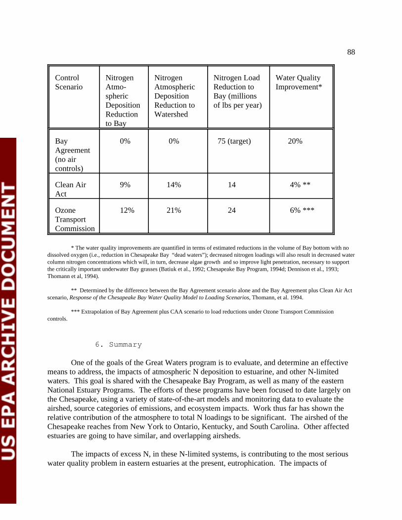
88

Control Nitrogen Nitrogen Nitrogen Load Water QualityScenario Atmo- Atmospheric Reduction to Improvement*

spheric Deposition Bay (millionsDeposition Reduction to of lbs per year) Reduction Watershedto Bay

Bay 0% 0% 75 (target) 20%Agreement(no aircontrols)

Clean Air 9% 14% 14 4% **Act

Ozone 12% 21% 24 6% ***TransportCommission

* The water quality improvements are quantified in terms of estimated reductions in the volume of Bay bottom with nodissolved oxygen (i.e., reduction in Chesapeake Bay “dead waters”); decreased nitrogen loadings will also result in decreased watercolumn nitrogen concentrations which will, in turn, decrease algae growth and so improve light penetration, necessary to supportthe critically important underwater Bay grasses (Batiuk et al., 1992; Chesapeake Bay Program, 1994d; Dennison et al., 1993;Thomann et al, 1994).

** Determined by the difference between the Bay Agreement scenario alone and the Bay Agreement plus Clean Air Actscenario, Response of the Chesapeake Bay Water Quality Model to Loading Scenarios, Thomann, et al. 1994.

*** Extrapolation of Bay Agreement plus CAA scenario to load reductions under Ozone Transport Commissioncontrols.

6. Summary

One of the goals of the Great Waters program is to evaluate, and determine an effectivemeans to address, the impacts of atmospheric N deposition to estuarine, and other N-limitedwaters. This goal is shared with the Chesapeake Bay Program, as well as many of the easternNational Estuary Programs. The efforts of these programs have been focused to date largely onthe Chesapeake, using a variety of state-of-the-art models and monitoring data to evaluate theairshed, source categories of emissions, and ecosystem impacts. Work thus far has shown therelative contribution of the atmosphere to total N loadings to be significant. The airshed of theChesapeake reaches from New York to Ontario, Kentucky, and South Carolina. Other affectedestuaries are going to have similar, and overlapping airsheds.

The impacts of excess N, in these N-limited systems, is contributing to the most seriouswater quality problem in eastern estuaries at the present, eutrophication. The impacts of

89

eutrophication range from increased turbidity shading out beneficial submersed aquaticvegetation habitats, to the exacerbation of noxious algae blooms, to the creation of low or no-oxygen conditions (hypoxia or anoxia) which negatively affect fish populations.

In the Chesapeake, the affected parties have agreed that a 40 percent reduction in Ninputs is needed for the Bay's health. The implementation of CAA provisions could account forabout a fifth to a third of that. These same actions would be expected to provide similar benefitsto yet unstudied estuaries with eutrophication problems.

References

Chesapeake Bay Program. 1995. Atmospheric Loadings to Coastal Areas: Resolving ExistingUncertainties. A report of the Atmospheric Loadings Workshop, Baltimore, Maryland June 29-30, 1994, organized and lead by the Air Quality Coordination Group and the Scientific andTechnical Advisory Committee of the Chesapeake Bay Program.

Chesapeake Executive Council. 1987. 1987 Chesapeake Bay Agreement. Annapolis, Maryland.

Chesapeake Executive Council. 1992. Chesapeake Bay Agreement 1992 Amendments.Annapolis, Maryland.

Chesapeake Executive Council. 1993. Directive 93-1 Joint Tributary Strategy Statement.Annapolis, Maryland.

Dennis, R.L. 1996. Using the Regional Acid Deposition Model to determine the nitrogendeposition airshed of the Chesapeake Bay watershed. In: J.E. Baker (ed.). AtmosphericDeposition of Contaminants to the Great Lakes and Coastal Waters. SETAC Press, Pensacola,Florida.

East Coast Atmospheric Resource Alliance. 1996. Airsheds and Watersheds - the Role ofAtmospheric Nitrogen Deposition. A report of the Shared Resources Workshop, October 11-12,1995, Warrenton, Virginia.

Fisher, D.C., J. Ceraso, T. Mathew, and M. Oppenheimer. 1988. Polluted coastal waters: the roleof acid rain. Environmental Defense Fund, New York, NewYork.

Linker, L.C., R.L.Dennis, and D.Y.Alegre. 1993. Inpact of the Clean Air Act on ChesapeakeBay Water Quality. International Conference on Environmental Management of EnclosedCoastal Seas. Baltimore, MD.

National Research Council. 1993. Report of the Committee on Wastewater Management forCoastal Urban Areas, Water, Science, and Technology Board. Washington, D.C.

Nixon, S.W. 1986. “Nutrient Dynamics and the Productivity of Marine Coastal Waters”. R.

90

Halwagy, D. Clayton, and M. Behbehani (eds): Coastal Eutrophication. pp 97-115. The AldenPress, Oxford.

Paerl, H.W. 1993. “The Emerging Role of Atmospheric Nitrogen Deposition in CoastalEutrophication: A Biogeochemical and Trophic Perspective.” Canadian Journal of Fisheriesand Aquatic Sciences. 50:2254-2269.

Paerl, H.W. 1995. “Coastal Eutrophication in Relation to Atmospheric Nitrogen Deposition:Current Perspectives.” Ophelia. 41:237-259.

Pechan, E.H. 1991. Background documentation on SO and NO forecasts. E.H. Pechan and2 x

Associates, Springfield, VA. EPA Contract No. 68-D00120.

Swain, W., T. Colborn, C. Bason, R. Howarth, L. Lamey, B. Palmer, and D. Swackhamer. 1994.Exposure and Effects of Airborne Contamination. U.S. Environmental Protection Agency. EPA-453/R-94-085.

Thomann, R.V., J.R. Collier, A. Butt, E. Casman, and L.C. Linker. 1994. Response of theChesapeake Bay Water Quality Model to Loading Scenarios. Chesapeake Bay Program Office,Annapolis, Maryland. CBP/TRS 101/94.

U.S. Environmental Protection Agency. 1994. National Water Quality Inventory: 1992 Report toCongress. Washington, D.C.

U.S. Environmental Protection Agency, Office of Air Quality Planning and Standards, revisedcriteria document, Air Quality Criteria for Oxides of Nitrogen (three volumes,EPA-600/8-91/049aF-cF, August 1993.

U.S. Environmental Protection Agency, Office of Air Quality Planning and Standards,Deposition of Air Pollutants to the Great Waters, Second Report to Congress, EPA-453/R-97-011, June 1997.

Valigura, R.A., J.E. Baker, J. R. Scudlark, and L.L. McConnell. 1995. Atmospheric Depositionof Nitrogen and Contaminants to Chesapeake Bay and its Watershed. In: Perspectives onChesapeake Bay, 1994: Advances in Estuarine Science. S. Nelson and P. Elliott, eds.Chesapeake Research Consortium, Edgewater, Maryland.

91

In order to compare the ability of a greenhouse gas over time to trap heat in the atmosphere relative14

to another gas, the concept of global warming potential (GWP) is used. The GWP uses carbon dioxide as thereference gas with a GWP of 1. Thus, emissions of greenhouse gases may be reported in terms of millionmetric tons of carbon equivalent over a century. N O, with a GWP of 320, has a much larger ability to trap2

heat than carbon dioxide on a gram for gram basis.

C. Global Warming

Global WarmingThe “greenhouse effect” is the name for the physical process whereby energy from the sun

passes through the atmosphere relatively freely, while heat radiating from the earth is partiallyblocked or absorbed by water vapor and other radiatively important gases in the atmosphere. Because the sun is hotter than the earth, its energy is radiated at a higher frequency which is notabsorbed well by gases such as carbon dioxide or water vapor. In contrast, these types of gasesare effective absorbers of the lower-frequency energy radiated by the earth. Since the“greenhouse” gases responsible for this selective absorption make up only about one percent ofthe atmosphere, they are also known as “trace” gases. The energy absorbed by the different tracegases can be calculated accurately. When the concentration of a trace gas increases, thisadditional absorption warms the planet, if there are no other changes in the climate system.

Greenhouse GasesNaturally occurring greenhouse gases include water vapor, carbon dioxide (CO ), methane2

(CH ), nitrous oxide (N O), and O (EPA, November 1995). In addition, other photochemically4 2 3

important gases--such as carbon monoxide, NO, NO and VOCs--are not greenhouse gases, but2

contribute indirectly to the greenhouse effect because they influence the rate at which O and3

other gases are created and destroyed in the atmosphere. That is, emissions of NO lead to thex

formation of tropospheric O , which is also a greenhouse gas. As described below, some3

important sources of NO are also emitters of N O. Since 1800, atmospheric concentrations ofx 2

carbon dioxide have increased by more than 25 percent, methane concentrations have doubled,and N O concentrations have risen approximately 8 percent; this recent atmospheric buildup2

appears to be largely the result of anthropogenic activities (EPA, October 1995).

Figure III-1 illustrates the relative contribution of the greenhouse gases to total UnitedStates anthropogenic emissions in 1994 (EPA, November 1995). Due largely to fossil fuelconsumption, carbon dioxide emissions accounted for the largest share of United States emissionson a carbon equivalent basis --almost 85 percent. Methane emissions accounted for 11 percent14

and N O emissions comprise about 2 percent of the global warming potential of all the United2

States greenhouse gases (EPA, November 1995). On a global basis,N O is estimated to2

contribute 6 percent of the total global warming atmospheric gases (Kramlich and Linak, 1994).

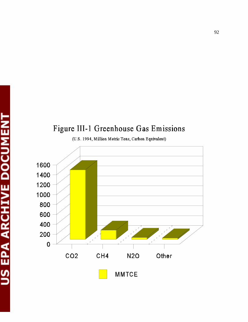
92

93

Denitrification is the process by which nitrates or nitrites are reduced by bacteria, which results in the escape15

of nitrogen into the air. Nitrification is the process by which bacteria and other microorganisms oxidize ammonium saltsto nitrites, and further oxidize nitrites to nitrates.

MMTCE is a method of comparing the global warming potential of various greenhouse gases. Carbon16

dioxide was chosen as the reference greenhouse gas.

N O2

N O is a chemically and radiatively active greenhouse gas that is produced naturally from a2

wide variety of biological sources in soil and water, as well as from various anthropogenicsources. With an atmospheric lifetime of 150 years, N O is extremely long-lived and very stable2

in the troposphere (Kramlich and Linak, 1994). While actual emissions of N O are much smaller2

than carbon dioxide emissions, N O is approximately 320 times more powerful than carbon2

dioxide at trapping heat in the atmosphere over a 100-year time horizon (EPA, November 1995).

N O Anthropogenic Emissions Sources2

N O is produced naturally in soils through the microbial processes of denitrification and2

nitrification . A number of anthropogenic activities add N to soils, thereby increasing the15

amount of N available for nitrification and denitrification, and ultimately the amount of N O2

emitted. Fertilizer use accounts for approximately 45 percent of total United States emissions ofN O. Anthropogenic emissions of N O in the United States have increased over 10 percent from2 2

1990 to 1994 primarily for two reasons: increased fertilizer use and general economic growth(EPA, October 1995). The major United States anthropogenic emissions sources are summarizedin the Figure III-2 (EPA, November 1995).

Other important anthropogenic activities producing N O are fossil fuel combustion from2

mobile and stationary sources, adipic acid production, and nitric acid production, whichcontribute 31, 13, and 10 percent, respectively, of the total United States emissions of N O. N O2 2

is a product of the reaction that occurs between nitrogen and oxygen during fossil fuelcombustion. Total emissions are estimated at approximately one half million tons or 41 millionmetric tons carbon equivalent (MMTCE) (EPA, November 1995). Mobile emissions totaled16

9.3 MMTCE in 1994, with road transport accounting for approximately 95 percent of these N O2

emissions. N O emissions from stationary fossil fuel combustion sources were 3.2 MMTCE in2

1994. Also with respect to 1994, the production of adipic acid (used to produce nylon)generated 5.4 MMTCE of N O. There are currently four plants in the United States that produce2

adipic acid. Since 1990, two of the plants have employed emissions control measures destroyingabout 98 percent of the N O before its release into the atmosphere. By 1996, all adipic acid2

production plants will have N O emissions controls in place as a result of a voluntary agreement2

among producers (EPA, November 1995). Production of nitric acid is another industrial sourceof N O emissions. Nitric acid is a raw material used primarily to make synthetic commercial2

fertilizer; N O emissions from this source were about 3.8 MMTCE in 1994.2

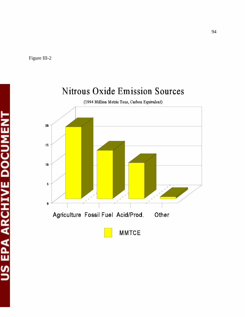
94

Figure III-2

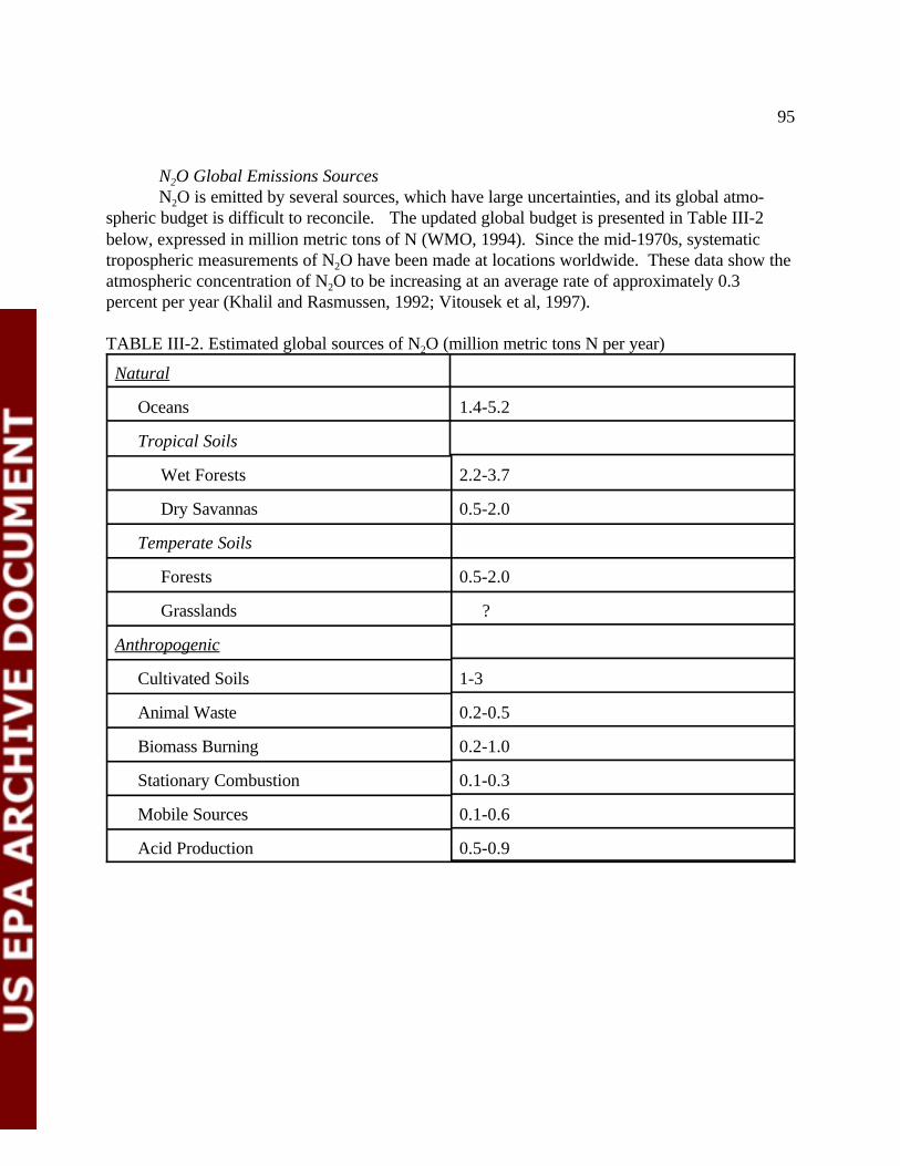
95

N O Global Emissions Sources2

N O is emitted by several sources, which have large uncertainties, and its global atmo-2

spheric budget is difficult to reconcile. The updated global budget is presented in Table III-2below, expressed in million metric tons of N (WMO, 1994). Since the mid-1970s, systematictropospheric measurements of N O have been made at locations worldwide. These data show the2

atmospheric concentration of N O to be increasing at an average rate of approximately 0.32

percent per year (Khalil and Rasmussen, 1992; Vitousek et al, 1997).

TABLE III-2. Estimated global sources of N O (million metric tons N per year)2

Natural

Oceans 1.4-5.2

Tropical Soils

Wet Forests 2.2-3.7

Dry Savannas 0.5-2.0

Temperate Soils

Forests 0.5-2.0

Grasslands ?

Anthropogenic

Cultivated Soils 1-3

Animal Waste 0.2-0.5

Biomass Burning 0.2-1.0

Stationary Combustion 0.1-0.3

Mobile Sources 0.1-0.6

Acid Production 0.5-0.9

96

O3

O is an important greenhouse gas present in both the stratosphere and troposphere. 3

Although representing only 10 percent of the total O column, tropospheric O is important3 3

because it can influence climate, as it is a greenhouse gas itself, and because its photolysis by UVradiation in the presence of water vapor is the primary source for hydroxyl radicals (WMO,1994). Hydroxyl radicals are responsible for the oxidative removal of many trace gases, such asmethane, hydrofluorocarbons, and hydrocholorfluorocarbons that influence climate and/or areimportant for the stratospheric O layer. 3

Observations show that free tropospheric O has increased above many locations in the3

Northern Hemisphere over the last 30 years. Model simulations and the limited observationstogether suggest that tropospheric O may have doubled in the Northern Hemisphere since pre-3

industrial times. Such changes in O have potentially important consequences for warming,3

although detailed quantification is not possible due to uncertainties in the size and distribution ofthe O change (Houghton, 1994). 3

Emissions of NO lead to the formation of tropospheric O . The increases in troposphericx 3

O will be regional in nature and so will the associated effects noted above. Because changes in3

the tropospheric O are highly spatially variable, both regionally and vertically, assessment of3

global long-term trends is extremely difficult. To the extent reductions in emissions of NO wouldx

lower tropospheric O concentrations, the global warming effects of tropospheric O would also3 3

be lowered.

Emissions Control ProgramsWhile the goal of many NO control procedures for mobile and stationary sources is tox

convert NO into N , some NO control programs strive to prevent NO emissions in the first2 x x

place. For example, efforts to lower miles traveled by vehicles or agricultural methods todecrease the amount of N fertilizer applied will decrease both NO and N O. Other controlx 2

programs are directed at N O emissions, such as in adipic acid production. However, many NO2 x

control procedures for mobile and stationary sources convert NO into N and, in that process, a2

portion of the reactions will form N O. Therefore, the development of an emissions control2

program to achieve a specific environmental goal may need to take into account the impact onboth NO and N O emissions and the resultant environmental impacts that may go beyond thex 2

specific goal.

The amount of N O emitted is generally small compared to the NO emissions reductions2 x

and varies, depending upon fuel, technology type, and pollution control device. Emissions alsovary with the size and vintage of the combustion technology, as well as maintenance andoperation practices. Staged combustion, including low-NO burners, and reburn technologiesx

have only a small influence on N O. In selective non-catalytic reduction, use of NH results in less2 3

than 5 percent of the NO reduced being converted to N O; use of urea converts more than 102

percent of the NO. The application of selective catalytic reduction suggests that N O emissions2

are negligible from vanadium catalysts; noble metal catalysts, however, may convert significant

97

quantities of NO into N O (Kramlich and Linak, 1994). Regarding mobile sources, as catalytic2

converter-equipped vehicles have increased in the United States motor vehicle fleet, emissions ofN O from this source have also increased (EPA, 1995). 2

References:

Houghton, J. T., et al, Climate Change 1994, “Radiative Forcing of Climate Change,” reports ofworking groups I and III of the Intergovernmental Panel on Climate Change, CambridgeUniversity Press, section 6.2.

Khalil, M.A. and Rasmussen, R.A., “The Global Sources of Nitrous Oxide,” J. Geophys. Res. 97, 14651-14660, 1992.

Kramlich, J.C. and Linak, W.P, “Nitrous Oxide Behavior in the Atmosphere, and in Combustionand Industrial Systems,” Prog. Energy Combust. Sci., Vol 20, 1994.

U.S. Environmental Protection Agency, Office of Policy, Planning and Evaluation, Inventory ofU.S. Greenhouse Gas Emissions and Sinks: 1990-1994, November 1995, EPA-230-R-96-006.

U.S. Environmental Protection Agency, Office of Air Quality Planning and Standards, NationalAir Pollutant Emission Trends, 1900-1994, October 1995, EPA-454/R-95-011.

usek, P.M., J. Aber, R.W. Howarth, G.E. Likens, P.A. Matson, D.W. Schindler, W.H.Schlesinger, and G.D. Tilman, “Human Alteration of the Global Nitrogen Cycle: Causes andConsequences,” Issues in Ecology, Number 1, Spring 1997.

World Meteorological Organization, Scientific Assessment of Ozone Depletion: 1994, GlobalOzone Research and Monitoring Project--Report No. 37.

98

D. Stratospheric Ozone Depletion

Stratospheric O3

O is mainly found in two regions of the Earth’s atmosphere. Over 90 percent of3

atmospheric O resides in the stratosphere, a layer between approximately 15 and 50 km (about3

10-30 miles) above the Earth’s surface (Kramlich and Linak, 1994). This stratospheric O is3

commonly known as the “ozone layer.” The remaining O is in the lower region of the3

atmosphere, the troposphere, which extends from the Earth’s surface up to about 10 km. Concentrations of O in the stratosphere are maintained by the balance between photochemical3

production of O (by photolysis of molecular oxygen, O ) and destruction of O . Stratospheric O3 3 32

is produced by the photolysis of O , which gives oxygen atoms (O), which then react with O to2 2

form O . Photochemical reactions associated with hydrogen oxides (HO ), NO , and halogen3 x x

oxides (ClO and BrO ) destroy O . The relative contribution of each to O destruction variesx x 3 3

with such factors as altitude, latitude, and season (WMO, 1994).

Stratospheric O plays a beneficial role by absorbing most of the biologically damaging3

ultraviolet sunlight called UV-B, allowing only a small amount to reach the Earth’s surface. Many experimental studies of plants and animals, and clinical studies of humans, have shown theharmful effects of excessive exposure to UV-B radiation. In contrast, at the planet’s surface, highconcentrations of O are toxic to living systems and can damage the tissues of plants and animals. 3

The ground-level O concentrations in the smoggiest cities are very much smaller than the3

concentrations routinely found in the stratosphere (WMO, 1994).

Stratospheric O Depletion3

Decreases in stratospheric O have occurred since the 1970s. The most obvious feature is3

the annual appearance of the Antarctic O hole in September and October. The October average3

total O values over Antarctica are 50-70 percent lower than those observed in the 1960s; this3

phenomenon has come to be known as the Antarctic “ozone hole.” The O loss occurs at3

altitudes between about 14 and 24 km. Smaller, but still significant losses in global total-columnO have also been observed in the more populated mid-latitudes (30-60 degrees) of both3

hemispheres (WMO, 1994). For example, in the middle latitudes of the Northern Hemisphere,downward trends of about 6 percent per decade over 1979-1994 were observed in winter andspring and about 3 percent per decade were observed in summer and fall.

Polar RegionsThe principal cause of O loss in the polar regions is photochemistry involving the halogen3

species, chlorine and bromine (WMO, 1994). Long-lived halogen species, primarilychlorofluorocarbons, are released in the troposphere from human activities. The photochemicaldegradation of these organic source molecules in the stratosphere leads to the formation of

99

inorganic halogen species. The release of chlorine from these species occurs in high-latitudewinter in reactions on surfaces of stratospheric aerosol particles. The formation and reactivity ofthese particles are enhanced at the low temperatures characteristic of the interior of the polarvortices. The removal of reactive nitrogen, especially nitric acid, by aerosol particlesedimentation in the vortex strongly regulates the rate of recovery by controlling the availability ofactive chlorine. In the Antarctic, weather patterns result in the annual polar vortex, whichprevents the transport of O from the southern hemisphere mid-latitudes to the polar regions,3

primarily in September and October.

Mid-latitudes As noted above, stratospheric O concentrations are lowered by photochemical reactions3

associated with the hydrogen, N, chlorine and bromine radicals. The concentrations of theseradical species are maintained by photodegredation of the corresponding source gases: H O and2

methane for HO , N O for NO , and halogen source gases for ClO and BrO . Increases in radicalx 2 x x x

concentrations (e.g., increases in ClO due to chloroflurocarbons emitted at the Earth’s surface,x

and increases in NO due to N O emitted at the ground and stratospheric injection of NO byx 2 x

aircraft) lead to changes in O (WMO, 1994).3

In the low stratosphere (10-22 km), reactions involving HO dominate the O loss rate,x 3

while between 23 and 40 km, NO cycles dominate (WMO, 1994). Decreases in NO abovex x

about 22 km, where it represents the dominant photochemical loss mechanism, would result inlocal stratospheric O increases (Tie et al, 1994). The broad picture is of reactions involving HO3 2

being responsible for over half the photochemical destruction of O in the low stratosphere at mid-3

latitudes, while halogen (chlorine and bromine) chemistry accounts for a further third. Althoughcatalytic destruction by NO accounts for less than 20 percent of the photochemical O loss in thex 3

low stratosphere at mid-latitudes, NO and NO are vital in regulating the abundance of hydrogen2

and halogen radicals and thus the total photochemical O destruction rate (WMO, 1994).3

It should also be noted that there is observational evidence that tropospheric O (about 103

percent of the total-column O ) has increased in the Northern Hemisphere (north of 20 degrees N)3

over the past 3 decades (WMO, 1994). The upward trends are highly regional. Tropospheric O3

(and aerosols) can decrease global UV-B irradiances. However, recent trends in troposphericpollution probably had only minor effects on UV trends relative to the effect of stratospheric O3

decreases (WMO, 1994).

N O2

The major sources of N O emissions are described in the “Global Warming” section of this2

document. As noted previously, N O has an atmospheric lifetime of 150 years. The major sink of2

N O is photo dissociation following diffusion into the stratosphere (WMO, 1994). Its products of 2

dissociation are the major source of stratospheric NO , which are important in regulatingx

stratospheric O . The dissociation produces NO, which leads to the subsequent chemical3

destruction of stratospheric O (Kramlich and Linak, 1994). Formation of NO in the stratosphere3

is the result of photolysis of N O and reaction with an oxygen atom. The NO formed2

100

subsequently reacts with stratospheric O , forming oxygen (O ). The net effect is that increased3 2

global concentrations of N O contribute to the thinning of the stratospheric O layer (Vitousek,2 3

1997).

N O is emitted by natural and anthropogenic sources, which are listed in Table III-2 and2

have large uncertainties. Stratospheric O destruction is further complicated by potential3

interaction between chlorine monoxide and NO , which may decrease stratospheric O destruction2 3

by interfering with atomic chlorine formation (Kramlich and Linak, 1994). Since the mid-1970s,systematic tropospheric measurements of N O have been made at locations worldwide. These2

data show the atmospheric concentration of N O to be increasing at an average rate of2

approximately 0.3 percent per year (Khalil and Rasmussen, 1992; Vitousek et al, 1997)).

NOx

Emissions from aircraft are a relatively small source of NO The impact of the aircraftx.

emissions depend on the altitude as well as the amount of the emissions. Models indicate that theNO emissions from the current subsonic fleet produce upper-tropospheric O increases as muchx 3

as several percent, maximizing at northern midlatitudes. In contrast, projected fleets ofsupersonic aircraft may decrease total-column O concentrations by 0.3-1.8 percent for the3

Northern Hemisphere (WMO, 1994).

Emissions Control ProgramsAs noted in the previous section concerning global warming, the development of an

emissions control program to achieve a specific environmental goal may need to take into accountthe impact on both NO and N O emissions and the resultant environmental impacts that may gox 2

beyond the specific goal. Some NO control programs strive to prevent NO emissions in the firstx x

place. Other control programs are directed at N O emissions, such as in adipic acid production. 2

However, many NO control procedures for mobile and stationary sources convert NO into Nx 2

and, in that process, a portion of the reactions will form N O. 2

References

Kramlich, J.C. and Linak, W.L, “Nitrous Oxide Behavior in the Atmosphere, and in Combustionand Industrial Systems,” Prog. Energy Combust. Sci., Vol 20, 1994.

Levine, J.S., “The Global Atmospheric Budget of Nitrous Oxide, and Supplement: GlobalChange: Atmospheric and Climatic,” 5th International Workshop on Nitrous Oxide Emissions,Tsukuba, Japan, 1992.

Khalil, M.A. and Rasmussen, R.A., “The Global Sources of Nitrous Oxide,” J. Geophys. Res. 97, 14651-14660, 1992.

Tie, X.X., G.P. Brasseur, B. Briegleb, and C. Grainier, “Two-Dimensional Simulation ofPinatubo Aerosol and Its Effect on Stratospheric Ozone,” J. Geophys. Res., 99, 20545-20562,1994.

101

Vitousek, P.M., J. Aber, R.W. Howarth, G.E. Likens, P.A. Matson, D.W. Schindler, W.H.Schlesinger, and G.D. Tilman, “Human Alteration of the Global Nitrogen Cycle: Causes andConsequences,” Issues in Ecology, Number 1, Spring 1997.

U.S. Environmental Protection Agency, Office of Policy, Planning and Evaluation, Inventory ofU.S. Greenhouse Gas Emissions and Sinks: 1990-1994, November 1995, EPA-230-R-96-006.

World Meteorological Organization, Scientific Assessment of Ozone Depletion: 1994, GlobalOzone Research and Monitoring Project--Report No. 37.

102

E. Terrestrial Ecosystems

N DepositionOver the last 40 years, the rate atmospheric deposition of N compounds has increased

more than 10 times in eastern North America (Vitousek, 1994). N accumulates in watershedswith high N deposition. The primary sources of N (NO and ammonia, NH ) deposition are thex 3

combustion of fossil fuels, the manufacture and use of fertilizers, livestock, and burning ofbiomass as a result of changing land use practices (Townsend, et al, 1996; Schlesinger andHartley, 1992). Because North American terrestrial ecosystems are generally considered to be N-limited, N deposition often has a fertilizing effect, accelerating plant growth. While this effect isoften considered beneficial, N deposition is causing important adverse changes in some terrestrialecosystems, including shifts in plant species composition and decreases in species diversity orundesirable nitrate leaching to surface and ground water and decreased plant growth.

The N CycleAll organisms require N to live; it is an essential component of cholorphyll, genetic

material, and proteins. In many ecosystems on land and sea, the supply of N is a key factorcontrolling the nature and diversity of plant life, the population dynamics of both grazing animalsand their predators, and vital ecological processes such as plant productivity and the cycling ofcarbon and soil minerals (Vitousek et al, 1997).

Although the earth’s atmosphere is 78 percent N gas (in the form of the N molecule),2

most plants and animals cannot use the atmospheric N directly. Before plants can use N, it must2

be bonded (“fixed”) into inorganic compounds, mainly ammonium, NH , and nitrate, NO . 4 3+ -

There are both natural and anthropogenic processes that “fix” atmospheric N into these inorganic2

compounds.

The main natural source of N fixation is N fixing organisms. N fixing organisms includealgae and bacteria. The most important ones are bacteria that form symbiotic relationships withhigher plants, especially legumes. These bacteria manufacture an enzyme that enables them toconvert atmospheric N directly into plant-usable forms. Lightning is also a natural source of N2

fixation as conditions of high pressure and temperature allow N and O to combine and form into2 2

nitrates.

During the past century, human activities have at least doubled the rate of transfer ofatmospheric N to biologically usable forms (Vitousek et al, 1997; Schlesinger, 1992). The major2

anthropogenic sources include industrial processes that produce N fertilizers, the combustion offossil fuels, and the cultivation of legumes. Furthermore, biomass burning, drainage of wetlandsand land clearing are important activities that contribute to biologically available N. Most of this

103

N is deposited by precipitation over land, where it enters biogeochemical cycles (Schlesinger,1992).

N Deposition Effects on Forest EcosystemsRates of growth in North American forest ecosystems have traditionally been considered

limited by N availability and, thus, N inputs are usually considered beneficial. In N-limited forests,most N is bound in soil organic matter and only becomes available for biotic uptake whendecomposition of soil organic matter releases inorganic nitrate and ammonium ions. Plants andmicrobes promptly absorb inorganic N, maintaining minimal available N pools in the soil andthereby limiting leaching losses. Although N limitation is still widespread, recent findings inNorth America and Europe suggest that, because of chronic N deposition from air pollution, someforests are no longer N-limited and that this condition may increase tree mortality and alter waterquality (Aber et al, 1996; Sullivan, 1993; Vitousek et al, 1997).

N saturation has a complex cascade of damaging effects for ecosystems (Vitousek et al,1997). As NH builds up in the soil, it is increasingly converted to nitrate, a process that releases4

+

hydrogen ions and helps acidify the soil. The buildup of nitrate may result in leaching of nitrateinto streams or groundwater. As negatively charged nitrates leach away, they carry with thempositively charged alkaline minerals, thus decreasing soil fertility. As calcium is depleted and thesoil acidified, aluminum ions are mobilized, eventually reaching toxic concentrations that candamage tree roots or kill fish if the aluminum washes into streams.

The impacts of N saturation first became apparent in Europe almost two decades agowhen scientists observed significant increases in nitrate concentrations in some lakes and streamsand also extensive yellowing and loss of needles in spruce and other conifer forests subjected toheavy N deposition (Vitousek et al, 1997). In Southern California, elevated nitrate and NO fluxesfrom soil, indicators of N saturation, have recently been reported for chaparral watersheds in theSan Gabriel Mountains as well as in portions of the mixed conifer forest in the San BernardinoMountains (Fenn et al, 1996). While there are important differences in the magnitude of Ndeposition, vegetation and soil cover, areas of concern include the Great Smoky Mountains inNorth Carolina, northeastern United States, southern California, and the Colorado Front Range ofthe Rocky Mountains (Johnson et al, 1991; van Miegroet et al, 1993; Fenn et al, 1996; Williamset al, 1996; Vitousek et al, 1997). In some cases excess N availability can lead to decreased treegrowth and increased mortality (McNulty et al.1996). Nutrient imbalances, with signs such asdepressed Ca:Al and Mg:N ratios in foliage, may act with other stresses to produce these effects(Aber et al. 1996).

N saturation has been defined in several ways, including, as a condition in which (1)available N is frequently in excess of total biotic demand, (2) vegetation within an ecosystem nolonger exhibits a positive growth response to N addition, even through other growth factors arenot growth limiting, and (3) sustained N losses approximate or exceed N inputs--the N retentioncapacity of the system has been exceeded (Fenn, et al, 1996). Recent research suggests thatbecause N-limited forests retain most N inputs, N deposition above relatively low amounts to

104

these systems is largely cumulative (Ryan, 1996). Moreover forests respond nonlinearly tocumulative N inputs if elevated N deposition continues over long periods. That is, N inputs to N-limited forests (with little accumulated N) stimulate their growth and those inputs are stronglyretained with little nitrate leaching. After N inputs have accumulated (to cause N saturation), theresponse of the forest changes so that N deposition increases nitrate leaching and may decreaseforest growth. In order to predict how an ecosystem will respond to N deposition one needs toknow where the ecosystem is on this response curve to cumulative N inputs. Predictions areuncertain about how much cumulative N inputs it will take over what time period to bring aboutN saturation in particular forest ecosystems because processes controlling N accumulation andloss are not completely understood and because data on the current stage of N saturation arelacking for most forests.

N Deposition Effects on Grassland EcosystemsReduced Species DiversityMost natural ecosystems have been N limited. Accordingly, native plant species have

adapted to this environmental constraint. With an increase in N deposition, many of the nativeplant species may no longer be able to compete with other species that are adapted to high Nconditions.

N deposition in grassland ecosystems has been shown to (1) alter the composition of thegrassland species in the affected area, (2) decrease species diversity, and (3) increase the aboveground productivity (Wedin and Tilman, 1996). In a 12 year experimental study of N depositionon Minnesota grasslands, plots dominated by native grasses shifted to low-diversity mixtures at allbut the lowest N addition rates (Wedin and Tilman, 1996). While prairie grasses can thrive wereN availability is limited, as N availability is increased, competing, non-native species begininvading the prairie plots. After 12 years of N addition, species richness (number of plant speciesper area) declined by more than 50 percent, with the greatest losses at levels spanning currentatmospheric deposition rates in eastern North America (Wedin and Tilman, 1996). That is, thenative grasses with supplemental N deposition showed an impaired ability to compete with non-native species. In England, N fertilizers applied to experimental grasslands led to increaseddominance by a few N responsive grasses and loss of many other plant species; at the highestfertilization rate, the number of plant species declined more than fivefold (Vitousek et al, 1997).

Global Warming ImpactsBecause plants use atmospheric carbon dioxide to fix carbon in their tissues, over their

lifetime they are a sink for atmospheric carbon dioxide, the primary global warming gas. As theplants die and decompose, a portion of the carbon returns to the atmosphere and a portion may beincorporated into the soils, resulting in a net sink of carbon dioxide. With increased N inputs andresulting increased plant growth, it has been hypothesized that the amount of carbon removedfrom the atmosphere might increase.

There is considerable uncertainty over both the magnitude and persistence of any N-derived carbon sink. Different ecosystem types vary greatly in their potential for carbon storage.

105

Much of the area experiencing high N deposition is covered by grasslands or cultivated areas. Ingeneral, N deposition that stimulates wood production will cause a relatively large and long-termremoval of carbon from the atmosphere. In contrast, foliar biomasses in forests and grasslandshave much more limited capacity for carbon storage and deposition onto cultivated areas is notlikely to contribute to any terrestrial sink (Townsend, et al, 1996).

In the case of the native prairie grasses, the decomposition is slow, resulting in the storageof carbon in the earth. In contrast, the non-native plants which thrive on N (and replace nativeplants under increased N deposition), decompose rapidly due to their high N content and, thus,return most of their carbon to the atmosphere, where it can contribute to global warming. The 12year study indicates that the carbon storage, in some plots, was decreased by 50 percent andconcludes that N-caused shifts in species composition limit the ability of temperate grasslands toserve as significant long-term carbon stores (Wedin and Tilman, 1996). Thus, N depositionshifted the mix of plants toward the faster growing non-native species which decreased the area’sability to move carbon dioxide from the air and store it in the soil.

References:

Aber, John D., Knute J. Nadelhoffer, Paul Steudler, and Jerry M. Melillo. 1989. NitrogenSaturation in Northern Forest Ecosystems. BioScience Vol. 39 No. 6. June, 378-386 .

Aber JD, Melillo JM, Nadelhoffer KJ, Pastor J, Boone RD. 1991. “Factors controlling nitrogencycling and nitrogen saturation in northern temperate forest ecosystems.” Ecol. Appl. 1:305-315

Aber, J.D., A. McGill, S. G. McNulty, R.D. Boone, K.J. Nadelhoffer, M. Downs,R. Hallett. “Forest biogeochemistry and primary production altered bynitrogen saturation.” Water, Air, & Soil Pollution, volume 85 (p.1665-1670),1995.

Agren GI, Bosatta E. 1988. Nitrogen saturation of terrestrial ecosystems .Environ. Pollut.54:185-97.

Christ M, Zhang Y, Likens GE, Driscoll CT. 1995. Nitrogen retention capacity of a northernhardwood forest soil under ammonium sulfate additions. Ecol. Appl. 5:802-12.

Fenn, M., M.A. Poth, D.W. Johnson. “Evidence for nitrogen saturation in the San BernardinoMountains in Southern California,” Forest Ecology and Management 82 ( p. 211-230), 1996.

McNulty, S.G., J.D. Aber, S.D. Newman. 1996. Nitrogen saturation in a highelevation New England spruce-fir stand. Forest Ecology and Management84:109-121.

Ryan, Douglas F., J.D. Aber, J.S. Baron, B.T. Bormann, C.T. Driscoll, M.E. Fenn, D.W.Johnson, A.D. Lemly, S.G. McNulty, and R. Stottlemyer, “Nitrogen Deposition from AirPollution: Implications for Forest Ecosystems in North America” draft 1996.

106

Schlesinger, W.H., Biogeochemistry: An Analysis of Global Change, 1991.

Schlesinger, W.H. and Hartley, A.E., “A Global Budget for Atmospheric NH ", Biogeochemistry3

15: 191-211, 1992.

Stoddard JL. 1994. Long-term changes in watershed retention of nitrogen: Its causes andaquatic consequences. In: Environmental Chemistry of Lakes and Reservoirs, Advances inChemistry Series No. 237, ed. LA Baker, pp. 223-284, Washington, DC: Amer. Chem. Soc.

Sullivan,T.J. 1993. “Whole ecosystem nitrogen effects research in Europe.” EnvironmentalScience & Technology 37:1482-1486.

Townsend, A.R., B.H.Braswell, E.A.Holland, and J.E.Penner, “Spatial and Temporal Patterns inTerrestrial Carbon Storage Due to Deposition of Fossil Fuel Nitrogen,” Ecological Applications,6(3), 1996 pp. 806-814, 1996.

Van Sickle, J. and M.R. Church. 1995. Methods for estimating the relative effects of sulfur andnitrogen deposition on surface water chemistry. EPA Rep. no. EPA/600/R-95/172. Washington, DC US Environ. Protect. Agency.121 pp.

Vitousek, P.M., J. Aber, R.W. Howarth, G.E. Likens, P.A. Matson, D.W. Schindler, W.H.Schlesinger, and G.D. Tilman, “Human Alteration of the Global Nitrogen Cycle: Causes andConsequences,” Issues in Ecology, Number 1, Spring 1997.

Wedin, David A. and David Tilman, “Influence of Nitrogen Loading and Species Composition onthe Carbon Balance of Grasslands.” Science, Volume 274, December 6, 1996.

Williams, Mark W., Jill S. Baron, Nel Caine, Richard Sommerfield and Robert Sanford, Jr. 1996.“Nitrogen Saturation in the Rocky Mountains.” Environmental Science & Technology Vol 30 No2.

Vitousek, P.M., Ecology, Volume 75 (1861),1994.

107

F. Toxic Products

IntroductionIn the atmosphere, NO reacts with common hydrocarbons and O to form a wide varietyx 3

of toxic compounds. Shepson et al. (1987) reported that photochemical reactions in a laboratorysmog chamber substantially increased the mutagenicity of such mixtures. This addedmutagenicity, measured by Ames assays, was time-dependent and associated mostly with the gasphase. The mutagenic transformation products were also refractory, accumulating and persistingin the chamber for hours after their production.

The accumulation of new mutagens by photochemically-mediated nitrate reactions raisessignificant public health concerns. Chemicals that are able to alter bacterial genes (DNA) alsohave the potential to cause mutations in higher organisms, and some fraction of these mutationsmay initiate carcinogenesis. Examples of transformation products thought to contribute toincreased mutagenicity include the nitrate radical, peroxyacetyl nitrate, nitroarenes, andnitrosamines (Shepson et al., 1987; CARB, 1986). Toxicological data on many of thesecompounds are limited, making it difficult to discuss effects of specific reaction products, but theoverall trend is well-established. Information on formation and toxicity of groups of substances issummarized below.

Nitrate RadicalThe gaseous nitrate radical is a product of the reaction of NO with O (Finlayson-Pitts2 3

and Pitts, 1993). This compound dissociates rapidly in sunlight, but it is possible that nighttimeconcentrations may become significant. Although health effects of the gaseous nitrate radicalhave not been described, radicals are generally highly reactive compounds with the potential todamage complex biological molecules such as proteins, lipids, and nucleic acids. Pitts et al.(1983) have postulated that the nitrate radical is capable of inducing genetic changes, but thisdoes not appear to have been tested in the laboratory.

Peroxyacetyl Nitrate (PAN)PAN (CH CO NO ) is an organic-nitrogenous air pollutant formed by complex3 3 2

photochemical reactions of common aliphatic compounds and NO . PAN has a relatively longx

thermal decomposition lifetime in the absence of NO. When NO is removed from the atmosphereby reaction with O , as in the afternoon and above the mixed layer at night, PAN can persist. 3

PAN is an important lacrimator, thought to contribute much of the eye-stinging effect of urbansmog. Tests for mutagenicity and carcinogenicity of pure PAN have not been reported in theliterature. However, Shepson et al. (1987) concluded that PAN formation accounted for asubstantial part of the increased mutagenicity observed in their smog chamber study.

108

NitroarenesButler et al. (1981) demonstrated that polynuclear aromatic hydrocarbons (PAHs) are

nitrated in the laboratory to form nitroarenes when exposed to concentrations of NO and nitric2

acid similar to those found in ambient air. These results suggest that PAHs (hydrocarbons havingmultiple carbon-ring structures, and major constituents of polycyclic organic matter) may also berapidly nitrated in the atmosphere. Rosenkrantz and Mermelstein (1983) reported similarreactions in PAHs adsorbed on soot particles and other substrates. Many of these compounds aremutagens and/or carcinogens, even when their parent non-nitrated PAH analogs are not. Examples from this broad spectrum of substances include nitrated analogs of quinoline, pyrene,fluorine, and naphthalene. Rosenkrantz and Mermelstein (1983) reported that many nitroarenesare potent bacterial mutagens and also produce a variety of genetic and genotoxic effects inmammalian cell assays, including unscheduled DNA synthesis, sister-chromatid exchange,chromosomal aberrations, gene mutations, and cell transformation. Data from whole animals arelimited, but various nitroarenes have produced skin tumors in mice and bladder tumors in dogsand monkeys.

NitrosaminesGehlert et al. (1979) reported the formation of nitrosamines (nitrated organic amine

compounds) from amines and NO in the laboratory, and proposed that this reaction also occursx

in the atmosphere. Although nitrosamines are rapidly decomposed by sunlight, ambientconcentrations could rise during the night. Nitrosamines are a major class of powerful chemicalcarcinogens, with different compounds sometimes exhibiting high target organ specificity inanimal studies. Sites of cancers induced by nitrosamines in rodents include the liver, bladder,lung, kidney, and pancreas (Casarett and Doull, 1986). Carcinogenesis occurs through metabolicactivation, followed by methylation of DNA by the electrophilic metabolites.

SummaryIn laboratory tests, nitrates react readily with common organic chemicals, and even O , in3

the presence of light to form a wide variety of mutagenic and carcinogenic transformationproducts. Although animal inhalation studies of individual compounds formed in this way arelimited, results of bacterial and mammalian cell bioassays indicate clearly that both mixtures andindividual mixture components are able to alter DNA. More research, especially whole animalstudies, would help the EPA understand the potential magnitude of public health impacts of thesetransformation products.

References

Butler, J.D. and P. Crossley. Atmospheric Environment. 15:91 (1981).

California Air Resources Board. The effects of oxides of nitrogen on California air quality. March 1986.

Casarett, I. and L.J. Doull. Toxicology. Macmillan Publishing Co., New York. C.D. Klaassen,M.O. Amdur, and J. Doull (eds.) (1986).

109

Finlayson-Pitts, B.J. and J.N. Pitts, Jr., “Atmospheric Chemistry of Tropospheric OzoneFormation: Scientific and Regulatory Implications,” Air and Waste Management Association,Vol. 43, August 1993.

Gehlert and W. Rolle. Experimentia 33:579 (1979).

Pitts, Jr. J.N., A.M. Winer, G.W. Harris, W.P.L. Carter, and E.C. Tuazon. Trace nitrogenousspecies in urban atmospheres. Environ. Health Perspectives 52:153-157 (1983).

Rosencrantz, H.S. and R. Mermelstein. Mutagenicity and genotoxicity of nitroarenes: allnitrogen-containing chemicals were not created equal. Mutation Research 114: 217-267 (1983).

Shepson, P.B., T.E. Kleindienst, and E.O. Edney. The production of mutagenic compounds as aresult of urban photochemistry. EPA 600/3-87/020 (1987).

110

IV. Interprogram Issues

A. Local and Regional NO Requirementsx

Policy Decisions Should Consider All the Effects of NO Emissionsx

As described in detail in sections II and III of this document, NO emissions impact thex

environment in a number of ways. Some of these are regional scale, adverse impacts. As noted inthe “Ozone” section, decreasing local NO emissions can, in some cases, increase local Ox 3

concentrations. This effect of NO emissions reductions must be carefully weighed against thex

multiple beneficial effects of NO emissions reductions with respect to acid deposition, drinkingx

water nitrate, eutrophication, global warming, NO , N in forest ecosystems, O , PM, stratospheric2 3

O depletion, toxics and visibility degradation. Further, the effects of emissions of N O are also of3 2

concern with respect to global warming and stratospheric O depletion. The EPA believes that3

policy decisions should be made considering the environment as a whole, rather than narrowlyviewing each program, one at a time. As stated by two committees of the National ResearchCouncil:

Changes in VOCs and NO will, because of their complex chemical interactions, also leadx

to changes in a variety of other pollutants associated with O , such as nitric acid,3

peroxyacetyl nitrate, NO , and aerosol particles. Some of these pollutants have known2

harmful effects on human health and welfare. Hence, it is important to recognize thatcontrol strategies implemented for O will simultaneously affect other species. (NRC,3

1991).

Visibility is just one of many air-quality problems. The pollutants that impair visibilitycontribute to other environmental problems, some of which have been or are beingconsidered as objects of federal, state, or local legislation or regulation. For example,controls aimed at decreasing acid deposition or lowering ambient concentrations of O and3

PM could improve visibility in Class I areas; conversely, controls aimed at improving10

visibility could alleviate other air-quality problems. Policy makers should weigh theselinkages in the design and assessment of possible control strategies. (NRC, 1993).

The remainder of this section primarily describes (1) the effects of NO emissionsx

reductions on O concentrations, (2) CAA requirements for NO controls in certain areas, (3)3 x

EPA action to waive these requirements in certain cases, and (4) the need for regional scale NOx

controls in the future for purposes of O attainment. Although the focus of the discussion is on3

O , EPA intends to use its discretion wherever possible to assure that policy decisions concerning3

O are consistent with other environmental goals which may suggest the need for reductions in3

NO emissions. The EPA believes that effective O control requires an integrated strategy thatx 3

111

combines cost-effective reductions in emissions at the local, state, regional, and national levels.

Role of NO and VOCs in Urban Ox 3

Great progress has been made over the past two decades, at the local, state and nationallevels in controlling emissions from many sources of air pollution. During this period, control ofVOCs was the main strategy employed in efforts to lower ground-level O . The 1970 and 19773

amendments to the CAA did not explicitly require NO emissions reductions from stationaryx

sources for purposes of attainment of the O standard. With respect to mobile sources, both VOC3

and NO emissions were decreased substantially. Scientific evidence at the time suggested thatx

VOC emissions reductions were preferred in most instances (EPA, 1993). The VOC controlapproach was reinforced by the fact that NO emissions decreases could in some cases increase Ox 3

concentrations.

More recently, it has become clearer that NO controls may be needed in many areas,x

especially areas where O concentrations continue to be high over a large region (as in the3

Midwest and Northeast). In the debate leading up to the 1990 CAA amendments, Congressincluded consideration of NO . A report by the Office of Technology Assessment (U.S.x

Congress, 1989) provided support for inclusion of NO controls in the O program. The 1990x 3

amendments changed the statutory framework to place NO emissions reductions on a more equalx

footing with the VOC emissions reductions.

In the process of adding these new NO requirements, Congress recognized that NOx x

emissions reductions would help achieve lower O concentrations in some O nonattainment areas,3 3

but that "there are some instances in which NO reductions can be of little benefit in reducing Ox 3

or can be counter-productive, due to the offsetting ability of NO to `scavenge' (i.e., react with)x

O after it forms" (H.R. Rep. No. 490, 101st Congress, 2nd Sess., at 204). The Congress3

provided for additional review and study under section 185B of the CAA "to serve as the basis forthe various findings contemplated in the NO provisions" (H.R. Rep. 490 at 257). x

Under section 185 of the CAA, the EPA, in conjunction with the National Academy ofSciences, conducted a study on the role of O precursors in tropospheric O formation which3 3

examined the role of NO and VOC emissions, the extent to which NO emissions reductions mayx x

contribute or be counterproductive to achieving attainment in different nonattainment areas, thesensitivity of O to the control of NO , the availability and extent of controls for NO , the role of3 x x

biogenic VOC emissions, and the basic information required for air quality models. The NASportion of the study was published in 1991 (NRC, 1991). The section 185B study was completedand submitted to Congress July 30, 1993 (EPA, 1993).

The 1991 National Academy of Sciences report recommends that “To substantially reduceO concentrations in many urban, suburban, and rural areas of the United States, the control of3

NO emissions will probably be necessary in addition to, or instead of , the control of VOCs.” x

The section 185B study concludes that the O precursor control effort should focus on NO3 x

controls in many areas and that the analysis of NO benefits is best conducted throughx

photochemical grid modeling. The shift to consideration of both NO and VOCs, explains thex

112

section 185B study, coincides with improved data bases and modeling techniques that provide theanalytical means to evaluate the effectiveness of O precursor control strategies. 3

The 1990 Clean Air Act Amendments (CAAA)The 1990 CAAA include substantial new requirements to decrease emissions of NO fromx

major stationary sources. To help attain the 1-hour O air quality standard in the near-term,3

section 182(f) of the CAAA requires certain existing sources to install reasonably availablecontrol technology (RACT) and new sources must install controls representing the lowestachievable emission rate (EPA, 1992). Section 182(f) also specifies circumstances under whichthe new NO requirements for RACT and NSR would be limited or would not apply. To decreasex

acid deposition, the CAAA require coal-fired utility boilers to meet emission limits in two phases. Further, in a longer-term provision, the CAAA require States to adopt additional controlmeasures as needed to attain the O standard. This requirement supplements the RACT and NSR3

requirements. Thus, a State would need to require NO controls which achieve emissionsx

reductions greater than the NO RACT/phase I acid deposition limits where additional reductionsx

in emissions of NO are necessary to attain the O standard by the attainment deadline.x 3

For O nonattainment areas designated as serious, severe, or extreme, state attainment3

demonstrations involve the use of photochemical grid modeling for each nonattainment area. Although these attainment demonstrations were due November 15, 1994, the magnitude of thismodeling task, especially for areas that are significantly affected by transport of O and O3 3

precursors (NO and VOCs) generated outside of the nonattainment area, has delayed many statesx

in submitting complete modeling results. Recognizing these challenges, EPA issued guidance onO demonstrations, based on a two-phase approach for the submittal of O SIP attainment3 3

demonstrations (Nichols, 1995). The guidance established a 2-phase approach which includes anintensive modeling effort to address the problem of long distance transport of O , NO and VOCs3 x

and submittal of the attainment plans in 1997.

Section 182(f) of the CAA--NO Waiverx

As described in EPA guidance (EPA, December 1993), the CAAA include new provisionsin section 182(f) to control emissions of NO and specify circumstances under which the new NOx x

requirements would be limited or would not apply. Section 182(f)(1) provides that certain newNO requirements shall not apply if the Administrator determines that any one of the followingx

tests is met:

(1) in any area, the net air quality benefits are greater in the absence of NO reductionsx

from the sources concerned;

(2) in nonattainment areas not within an O transport region, additional NO3 x

reductions would not contribute to O attainment in the area; or 3

(3) in nonattainment areas within an O transport region, additional NO reductions3 x

would not produce net O air quality benefits in the transport region.3

113

Further, section 182(f)(2) states that the application of the new NO requirements may be limitedx

to the extent necessary to avoid excess reductions of NO as determined by applying tests similarx

to tests (1)-(3) above.

Administrative ProceduresSection 182(f)(3) provides that a person may petition the Administrator for a NOx

exemption at any time after the final section 185B report is submitted to Congress. The finalsection 185B report was sent to Congress by the Administrator on July 30, 1993. The petitionmay be made with respect to any nonattainment area or any O transport region. The EPA must3

grant or deny a petition within 6 months after its filing.

If EPA grants a petition, the section 182(f)NO requirements or portions of thosex

requirements (EPA, 1992), would no longer apply to those sources or areas, as described inEPA's approval action. However, States remain free to adopt NO restrictions for other reasons. x

For example, a State may determine that NO emissions reductions are needed for purposes of Ox 3

maintenance planning, O attainment in separate downwind nonattainment areas, visibility3

protection, PM control strategy, acid deposition program or other environmental protection.

The CAA requires EPA to view NO waivers in a narrow manner. In general, sectionx

182(f) provides that waivers must be granted if states show that decreasing NO within ax

nonattainment area would not contribute to attainment of the O NAAQS within the same3

nonattainment area (Seitz, 1995). Only the role of local NO emissions on local attainment of thex

O standard is considered in nonattainment areas outside an O transport region. The role of NO3 3 x

in regional attainment will be addressed separately. As described in the “Ozone” section, NOx

has been shown to be effective in decreasing regionally transported O .3

Status of NO Waiver Petitionsx

In response to State NO waiver petitions submitted between 1992-1995, EPA grantedx

NO waivers under section 182. Most waivers were granted on the basis that the area had alreadyx

attained the O standard and, thus, additional NO (or VOC) reductions “would not contribute to3 x

ozone attainment in the area.” In some cases, the waivers were granted based on dispersionmodeling which showed that the area would attain just as expeditiously based solely on additionalVOC reductions or that local NO reductions increased local peak O concentrations; this alsox 3

meets the above test that additional NO reductions would not contribute to O attainment in thex 3

area.

Specifically, the EPA received petitions for a NO waiver for 51 O nonattainment areas. x 3

Of these petitions, EPA approved (as of July 1997) waivers for 48 nonattainment areas and 3were pending. Most of the waivers granted (28) were simply based on air quality monitoring dataover a period of 3 or more years indicating the area had attained the O standard (and, thus,3

additional NO reductions were not needed for attainment). Several States submitted NO waiverx x

petitions (7) accompanied by an attainment plan showing achievement of the O standard by the3

statutory deadline through additional VOC controls only. None of these 41 nonattainment areas

114

with approved NO waivers have demonstrated or even sought to demonstrate that NOx x

reductions might increase O concentrations in specific areas. Only in the cases of the Lake3

Michigan (9 nonattainment areas), Phoenix AZ, Baton Rouge LA and the Houston/Beaumont TXareas was information submitted to show that, on some days, local NO emissions decreases leadx

to local increases in peak O concentrations in some but not necessarily all portions of these areas. 3

Even for the 4 areas with modeling information, those analyses were generally consideredpreliminary analyses that would be replaced with more complete modeling associated withattainment plans.

NO waivers are granted on a temporary or contingent basisx

The EPA's approval of any NO exemption is granted on a contingent basis (Seitz, 1994).x

That is, a monitoring-based exemption lasts for only as long as the area's monitoring data continueto demonstrate attainment. Thus, if a violation is monitored (prior to the area being redesignatedas being in attainment) the exemption would need to be revoked and the requirement to adoptNO controls would again apply. Similarly, any modeling-based exemption may need to bex

withdrawn if updated modeling analyses reach a different conclusion than the modeling on whichthe exemption was based (EPA, 1992).

In the Federal Register notices approving individual waiver petitions, EPA gave noticethat approval of the local petition is on a contingent or temporary basis and stated that additionallocal and regional NO emissions reductions may be needed to reduce the long range transport ofx

O . Where such additional NO reductions are necessary to reduce the long range transport of O ,3 x 3

EPA stated that authority provided under section 110(a)(2)(D) of the CAA would be used andthat a section 182(f) NO waiver would, in effect, be superseded for those control requirementsx

needed to meet the section 110(a)(2)(D) action. Further, EPA noted that States may requireadditional NO reductions in these nonattainment areas for non-O purposes, such as attainment ofx 3

the PM-10 standard or achieving acid rain reduction goals.

In some cases, despite a potential increase in O concentrations in central urban areas,3

State and local agencies may need to decrease NO emissions as part of a larger plan to meetx

various environmental goals. For example, the South Coast area of California models this effect,yet substantial NO emissions reductions are contained in their attainment plan. The NOx x

emissions reductions in the South Coast are needed to attain the PM standard and to maintain10

the NO standard in the same air basin as well as to help lower O concentrations in areas2 3

downwind of the basin. In a different situation, NO emissions reductions in the New Yorkx

metropolitan area are needed for downwind areas within the State and in other States to attain theO standard; yet, additional VOC controls may be needed in the metropolitan area to offset the3

local impact of NO emissions reductions. Similarly, NO emissions reductions in areas upwind ofx x

the Northeast Ozone Transport Region may be needed to help downwind areas attain andmaintain the O standard, even though those NO emissions reductions may not help the upwind3 x

areas lower local O concentrations. Models provide a way to test various control strategies so3

that the best approach, considering all the environmental goals, can be selected.

115

Further, the NO waiver does not shield an area from the acid deposition requirements ofx

Title IV of the CAA. Regional and/or local NO emissions reductions may also be needed to slowx

eutrophication in sensitive water bodies, improve visibility and/or decrease PM concentrations. Furthermore, increases in NO are not viewed by EPA as a solution to local O problems; NOx x3

emissions reductions are generally needed at least to counter increases in NO emissions due tox

economic growth. Thus, a local NO waiver should be considered temporary and does not shieldx

an area from NO requirements needed for O attainment in downwind areas or to meet otherx 3

CAA requirements.

Modeling AnalysesThe OTAG addressed the complex issue of regional impacts due to transport of NO andX

VOC emissions. The OTAG modeling results indicate that urban NO reductions producex

widespread decreases in O concentrations on high O days. In addition, urban NO reductions3 3 x

also produce limited increases in O concentrations locally, but the magnitude, time, and location3

of these increases generally do not cause or contribute to high O concentrations. Most urban O3 3

increases modeled in OTAG occur in areas already below the O standard and, thus, in most3

cases, urban O increases resulting from NO reductions do not cause exceedance of the O3 x 3

standard. There are a few days in a few urban areas where NO reductions are predicted tox

produce O increases in portions of an urban area with high O concentrations. 3 3

In other words, modeling analyses conducted as part of the OTAG process indicated that,in general, NO reduction disbenefits are inversely related to O concentration. On the low Ox 3 3

days leading up to an O episode (and sometimes the last day or so) the increases are greatest, and3

on the high O days, the increases are least (or nonexistent); the O increases occur on days when3 3

O is low and the O decreases occur on days when O is high. This indicates that, in most cases,3 3 3

urban O increases may not produce detrimental effects. However, OTAG modeling indicates3

that at least one area for one day of one episode experienced an increase in O on a high O day. 3 3

Overall, OTAG modeling thus demonstrates that the O reduction benefits of NO control far3 x

outweigh the disbenefits of urban O increases in both magnitude of O reduction and geographic3 3

scope.

It should also be noted that the modeling analyses completed within the OTAG processnecessarily utilized a larger grid size than States are likely to use in their attainment plans. That is,future analyses by States will likely use smaller grid sizes. The smaller grid sizes should providemore precise information on effects such as local NO emissions reacting with local O . x 3

Furthermore, new work is on-going to analyze air quality monitoring data, in part, to assessweekday and weekend patterns that may relate changes in NO and VOC emissions to changes inx

O concentrations. These air quality modeling and monitoring studies will provide additional3

information that may be important as States develop their attainment plans.

Regional Transport of O 3

The problem of regional transport of O and its precursors is widely recognized by the3

States. In response to concerns about this problem raised by state environmental commissioners

116

comprising the Environmental Council of the States, EPA has worked closely with states in theOTAG to develop various recommended control measures intended to address the regional natureof O . Similarly, State and local air administrators passed a unanimous resolution endorsing3

national NO emission regulations (Becker, 1995).x

Control strategies need to consider efforts to decrease regional scale emissions as well aslocal emissions. In general, NO emissions decreases in upwind, rural areas coupled with VOCx

emissions reductions in urban nonattainment areas appears to be an effective strategy. In somecases however, the urban nonattainment area is also upwind of another urban nonattainment areaor biogenic VOC emissions are very high. In these cases, local NO emissions reductions may bex

needed in addition to VOC emissions reductions for purposes of O attainment. In both cases,3

decreases in precursor emissions in the upwind areas will help the downwind metropolitan areasattain and maintain the O standard. Thus, effective O control will require an integrated strategy3 3

that combines cost-effective decreases in emissions at the local, state, regional, and nationallevels. Specific regional perspectives on the need for an integrated strategy are described in the“Ozone” section.

References

Becker, William, Executive Director of STAPPA/ALAPCO, Letter to U.S. EPA Public Docket,October 13, 1995.

National Research Council, Committee on Haze in National Parks and Wilderness Areas,Protecting Visibility in National Parks and Wilderness Areas, 1993.

National Research Council, Committee on Tropospheric Ozone Formation and Measurement,Rethinking the Ozone Problem in Urban and Regional Air Pollution, 1991.

Nichols, Mary D., Assistant Administrator for Air and Radiation, U.S. Environmental ProtectionAgency, “Ozone Attainment Demonstrations,” memorandum to EPA Regional Administrators,March 2, 1995.

Ozone Transport Assessment Group, Joint meeting of RUSM & ISI workgroups, “First RoundStrategy Modeling,” October 25, 1996.

Seitz, John S., Director, Office of Air Quality Planning and Standards, U.S. EnvironmentalProtection Agency, "Section 182(f) Nitrogen Oxides (NO ) Exemptions—Revised Process andx

Criteria," EPA memorandum to Regional Air Directors, May 27, 1994.

Seitz, John S., Director, Office of Air Quality Planning and Standards, U.S. EnvironmentalProtection Agency, "Section 182(f) Nitrogen Oxides (NO ) Exemptions-- Revised Process andx

Criteria," EPA memorandum to Regional Air Directors, February 8, 1995.

US Congress, Office of Technology Assessment, Catching Our Breath: Next Steps for Reducing

117

Urban Ozone, Washington DC 1989.

U.S. Environmental Protection Agency, Office of Air Quality Planning and Standards, The Roleof Ozone Precursors in Tropospheric Ozone Formation and Control--A Report to Congress. EPA-454/R-93-024,1993.

U.S. Environmental Protection Agency, “Nitrogen Oxides Supplement to the General Preamblefor Implementation of Title I of the Clean Air Act,” Federal Register of November 25, 1992 (57FR 55620).

U.S. Environmental Protection Agency, Office of Air Quality Planning and Standards, “Guidelinefor Determining the Applicability of Nitrogen Oxides Requirements Under Section 182(f),”December 1993.

118

B. Timing of NO Emissions Reductions: Seasonal or Year-x

Round

Regulation Can Affect the Seasonal Distribution of NO Emissionsx

As noted previously, NO emissions have adverse impacts on the environment in severalx

ways. In some cases, the timing of the NO emissions can be important to the subsequent x

environmental impacts. As noted below, year-round reductions in NO emissions are morex

helpful than seasonal approaches at minimizing the impacts of acid deposition andeutrophication, while summertime NO emissions reductions are most helpful in attaining the Ox 3

standard. In some cases, PM nonattainment and visibility impacts are strongly related to10

seasonal conditions. Since regulatory programs may be designed to achieve emissions decreasesat a constant, year-round rate or on a seasonal basis, the impacts of the policy decisions on thetiming of the required decreases need to be understood and, to the extent possible, integrated.

NO Emissions by Seasonx

As shown in the table at the end of this section, total NO emissions vary somewhat byx

season, with summer emissions usually slightly highest (EPA, 1995). Several source categoriesemit evenly throughout the year. NO emissions from electric utilities are highest in thex

summer. On-road NO emissions vary little from season to season, but are slightly higher in thex

summer than winter. Non-road engine emissions (non-road diesel and gasoline) are higher in thesummer than in the winter since weather limits the use of these engines for construction, lawnand garden, recreation, and light commercial purposes.

Seasonal Considerations in Environmental ProgramsAcid DepositionThe impacts from acid deposition are both cumulative and short-term. The cumulative

effects are due to long-term chronic acidification of watersheds. In addition, some importantadverse effects are associated with springtime snowmelt. As described in section II.A of thisdocument, nitric acid deposition plays a dominant role in the acid pulses associated with the fishkills observed during the springtime melt of the snowpack in sensitive watersheds. Thus,wintertime NO emissions reductions are especially important to lessening the incidence andx

severity of acidic episodes in certain areas. In addition, the timing of aluminum concentrationpeaks is also important. Toxic aluminum peaks related to nitrate fluctuations commonly occur inlate summer or early fall when soil temperatures and root growth are usually high (Joslin et al.,1992). Continuous year-round NO emissions reductions appear to be the most beneficial forx

decreasing acid deposition damage to natural resources.

EutrophicationN is the limiting nutrient in most coastal estuaries and many lakes. Thus, as described in

119

section III.B of this document, addition of N results in accelerated plant growth in the waterbodycausing adverse ecological effects and economic impacts that range from nuisance algal bloomsto oxygen depletion and fish kills. Simulated water quality responses to year-round vs seasonalnutrient emissions reductions conducted as a 1992 reevaluation of the baywide Tributary NutrientReduction Strategy by the Chesapeake Bay Program indicated the need for year round controls onphosphorus and N loadings (Thomann et a. 1994).

Ground-level O3

High ambient concentrations of O are associated with periods of elevated temperature3

and solar radiation. Thus, in most parts of the country, high O episodes occur only during3

summer months. Accordingly, the control of NO emissions on a summer season basis may bex

part of some areas’ strategies to attain the O standard at least cost. It should also be noted that3

application of NO emissions controls that focus emissions reductions in the summer will, inx

many cases, also achieve significant emissions reductions on a year-round basis. For example,efforts to decrease emissions from large boilers will usually include installation of low NOx

burners--which will achieve year-round moderate amounts of emissions reductions--and mayinclude, in addition, some type of summer season control, such as switching to a cleaner fuel orpost-combustion technology. In some cases, year-round emissions reductions contained inStates’ O attainment plans are explicitly supplemented by seasonal requirements; e.g., the3

Northeast States adopted a strategy which calls for NO emissions reductions in three phasesx

over the region with Phase 1 requiring year-round controls and the subsequent phases coveringthe May through September timeframe.

NO 2

Since the NO NAAQS requires ambient concentrations to be averaged over an annual2

period, seasonal emissions should not affect this program.

PMIn some cases PM nonattainment is related to seasonal emissions. For example, in10

some mountain/valley locations, the burning of wood for heating purposes results in wintertimeexceedances of the NAAQS. In other cases, PM nonattainment is related to a variety of10

sources on a non-seasonal basis.

Visibility and Regional HazeVisibility is lowest in the summer in the region south of the Great Lakes and east of the

Mississippi; in some locations the light extinction is more than twice as great in the summer asduring the other seasons (NRC, 1993). The most intense regional haze in the US occurs in theeast, where summertime meteorological conditions associated with slow-moving high-pressuresystems create stagnant conditions (NRC, 1993). Thus, in the summer, pollutants from manydifferent sources can accumulate, causing severe and widespread visibility degradation.

In the Grand CanyonVisibility Transport Commission’s June 10, 1996 report it is notedthat seasons influence the relative visibility impacts of regional and local emissions. Bothemission types contribute to visibility impairment much of the year, and either type can be the

120

dominant cause of impairment on any particular day regardless of the season.

Example of Consideration of Seasonal Concerns in O Policy3

O Season Emissions Limit3

To help achieve the O standard, many areas require application of RACT on major3

stationary sources of NO . Typically these controls involve modifications to combustionx

equipment, such as installation of low NO burners. Such controls operate continuously, year-x

round.

EPA guidance issued in 1993 (Shapiro, 1993) gives States the option to allow sources tocontrol NO emissions by switching to cleaner fuels during the O season. The NO emissionsx x3

reductions must be equal to or greater than emissions reductions that would have occurred fromapplication of typical RACT controls. In general, a fuel-switching program would provide newflexibility to States and industry in meeting certain Act requirements, including the NO RACTx

requirements. Fuel switching is a viable option for units where natural gas is readily availablesince the price of natural gas in the O season may be competitive with other fuels.3

Fuel-Switching Environmental ConsiderationsThe EPA considered the relative environmental benefits for fuel switching and

presumptive NO RACT. In terms of the primary purpose of NO RACT, that is lowering Ox x 3

effects in areas of high concentrations, it is clear that the NO emissions reductions due tox

burning a cleaner fuel during the O season would be much more effective than lesser emissions3

reductions at the presumptive NO RACT levels, which would be evenly spread over an entirex

year. The use of natural gas instead of coal could also substantially decrease annual andsummertime emissions of SO , carbon dioxide (CO ), PM , and associated toxic emissions such2 2 10

as mercury. Further, emissions reductions of these pollutants may be especially effective in thesummer with respect to decreasing regional haze and sulfate-related PM, both of which tend topeak in the summer. Thus, the potential benefits that go beyond the title I O and NO RACT3 x

goals include helping attain/maintain the NAAQS for SO and PM, decreasing mercury and2

other air toxic emissions, improving visibility, and cutting emissions of CO , a global warming2

gas.

The EPA also considered evidence suggesting that, for certain ecosystems, decreases inN deposition that occur only during the summer would be less effective at decreasing aciddeposition and nutrient impacts than emissions reductions that occur more uniformly throughoutthe year. It is not possible at this time to determine or fully quantify this relative ecologicalimpact. Moreover, due to the inherent limits on the amount of fuel switching that can occur andthe required NO emissions reductions under the CAA, wintertime N deposition would bex

projected to decrease in most areas regardless of fuel switching. In contrast, the O related3

benefits--and many of the additional potential benefits of fuel switching noted above--are wellknown and quantifiable. In conclusion, it was EPA's judgment that substantial decreases in O3

concentrations would occur from fuel switching; this benefit and the accompanyingimprovements in visibility, PM, air toxics, and global warming that also occur from fuelswitching clearly outweigh the decreased year-round benefits.

121

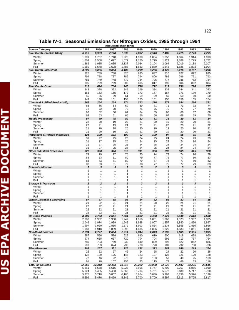
122

Table IV-1. Seasonal Emissions for Nitrogen Oxides, 1985 through 1994(thousand short tons)

Source Category 1985 1986 1987 1988 1989 1990 1991 1992 1993 1994Fuel Comb.-Electric Utility 6,916 6,909 7,128 7,530 7,607 7,516 7,488 7,475 7,773 7,795

Winter 1,801 1,757 1,748 1,928 1,980 1,804 1,858 1,864 1,914 1,913Spring 1,603 1,568 1,627 1,679 1,760 1,729 1,722 1,768 1,779 1,772Summer 1,862 1,935 2,055 2,137 2,034 2,104 2,064 2,019 2,188 2,207Fall 1,650 1,648 1,698 1,786 1,833 1,879 1,843 1,825 1,893 1,904

Fuel Comb.-Industrial 3,209 3,065 3,063 3,187 3,209 3,256 3,175 3,216 3,197 3,206Winter 825 789 788 820 825 837 816 827 822 825Spring 794 758 757 789 794 806 786 796 791 793Summer 785 749 748 779 784 796 777 786 782 784Fall 805 769 769 800 805 817 796 806 802 804

Fuel Comb.-Other 712 694 706 740 736 712 719 730 726 727Winter 343 328 332 349 349 334 338 344 341 343Spring 163 162 165 172 172 167 167 171 170 170Summer 56 56 59 61 59 59 59 60 60 60Fall 149 148 151 158 155 151 155 156 155 154

Chemical & Allied Product Mfg. 262 264 255 274 273 276 278 284 286 291Winter 65 66 64 69 69 71 71 73 73 74Spring 72 72 70 75 74 75 75 77 77 79Summer 62 62 60 64 64 65 65 66 67 68Fall 63 63 61 66 66 66 67 68 69 70

Metals Processing 87 80 75 82 83 81 78 80 81 84Winter 22 20 19 20 21 20 19 20 20 21Spring 22 21 19 21 21 21 20 20 21 22Summer 21 20 18 20 20 20 19 20 20 21Fall 21 20 19 20 21 20 19 20 20 21

Petroleum & Related Industries 124 109 101 100 97 100 97 96 95 95Winter 31 27 25 25 24 25 24 24 23 23Spring 31 27 25 25 24 25 24 24 24 24Summer 31 27 25 25 24 25 24 24 24 24Fall 31 27 25 25 24 25 24 24 24 24

Other Industrial Processes 327 328 320 315 311 306 297 305 315 328Winter 79 79 77 76 75 74 72 74 76 79Spring 83 83 81 80 79 77 75 77 80 83Summer 83 83 81 80 79 77 75 77 80 83Fall 82 83 81 79 78 77 75 77 79 83

Solvent Utilization 2 3 3 3 3 2 2 3 3 3Winter 1 1 1 1 1 1 1 1 1 1Spring 1 1 1 1 1 1 1 1 1 1Summer 1 1 1 1 1 1 1 1 1 1Fall 1 1 1 1 1 1 1 1 1 1

Storage & Transport 2 2 2 2 2 2 2 3 3 3Winter 1 1 1 1 1 1 1 1 1 1Spring 1 1 1 1 1 1 1 1 1 1Summer 1 1 1 1 1 1 1 1 1 1Fall 1 1 1 1 1 1 1 1 1 1

Waste Disposal & Recycling 87 87 85 85 84 82 83 83 84 85Winter 21 22 21 21 21 20 20 21 21 21Spring 22 22 21 21 21 21 21 21 21 21Summer 22 22 21 21 21 21 21 21 21 21Fall 22 22 21 21 21 21 21 21 21 21

On-Road Vehicles 8,089 7,773 7,651 7,661 7,682 7,488 7,373 7,440 7,510 7,530Winter 2,063 1,962 1,938 1,949 1,956 1,881 1,863 1,873 1,907 1,925Spring 2,046 1,974 1,939 1,942 1,938 1,907 1,857 1,880 1,896 1,897Summer 1,997 1,920 1,885 1,879 1,903 1,864 1,834 1,855 1,856 1,866Fall 1,983 1,918 1,889 1,892 1,885 1,836 1,820 1,833 1,851 1,841

Non-Road Sources 2,734 2,777 2,664 2,914 2,844 2,843 2,796 2,885 2,985 3,095Winter 587 596 574 625 610 610 600 618 638 660Spring 674 685 657 720 704 704 691 713 737 764Summer 780 793 759 830 810 809 796 822 852 886Fall 693 703 674 738 720 720 709 732 758 786

Miscellaneous 309 257 351 726 292 373 283 249 219 374Winter 25 22 27 46 24 28 24 22 20 28Spring 122 120 125 146 123 127 123 121 120 128Summer 72 46 92 278 62 103 57 40 25 103Fall 91 70 107 256 83 115 79 66 53 116

Total All Sources 22,860 22,348 22,403 23,618 23,222 23,038 22,672 22,847 23,276 23,615Winter 5,861 5,668 5,615 5,928 5,955 5,747 5,705 5,757 5,856 5,910Spring 5,624 5,485 5,483 5,665 5,704 5,761 5,572 5,680 5,717 5,760Summer 5,775 5,718 5,807 6,180 5,864 5,830 5,797 5,796 5,976 6,128Fall 5,599 5,476 5,499 5,845 5,700 5,700 5,597 5,613 5,725 5,817

123

References

Grand Canyon Visibility Transport Commission, Recommendations for Improving WesternVistas, June 10, 1996 report of the Grand CanyonVisibility Transport Commission to the UnitedStates Environmental Protection Agency, June 10, 1996.

National Research Council, Committee on Haze in National Parks and Wilderness Areas,Protecting Visibility in National Parks and Wilderness Areas, 1993.

Shapiro, Acting Assistant Administrator, Office of Air and Radiation, U.S. EnvironmentalProtection Agency, "Fuel Switching to Meet the Reasonably Available Control Technology(RACT) Requirements for Nitrogen Oxides (NO )” EPA memorandum to Regional Air Directors,x

July 30, 1993.

U.S. Environmental Protection Agency, Office of Air Quality Planning and Standards, NationalAir Pollutant Emission Trends, 1900-1994, October 1995, EPA-454/R-95-011.

124

C. Interface with Other Control Programs: Three Examples ofSecondary Emissions, EPA’s Clean Air Power Initiative, andNew Standards for O and Particulate Matter3

1. Synthetic Organic Chemical Manufacturing Industry (SOCMI)The CAA amendments of 1990 mandate that SIPs for certain O nonattainment areas be3

revised to require RACT to limit emissions of VOCs from sources for which EPA has published acontrol techniques guideline (CTG) document. Each CTG document contains a recommended"presumptive norm" for RACT for a particular source category, based on the EPA's currentevaluation of capabilities and problems general to the source category. In some cases, controlsfor VOCs could increase NO emissions (secondary emissions). In EPA’s development of thex

SOCMI CTG for Halogenated and Nonhalogenated Vent Streams (EPA, August 1993), this issuewas addressed. The CTG illustrates eight optional levels of control, with the NO secondaryx

emissions listed. In most options the amount of secondary NO emissions is extremely smallx

compared to the decrease in VOC emissions. In addition, the CTG addresses the issue ofsecondary emissions as follows:

Another important consideration in applying RACT is emission of pollutants such ascarbon monoxide and nitrogen oxides from combustion-based control devices. Thepotential consequences of emission from control devices are twofold. First, depending onthe VOCs-to-NO ratio in the ambient air, NO emissions from control devices may causex x

more O to be formed than could be eliminated through VOC emissions reductions. 3

Second, emissions from control devices may be enough to trigger New Source Review. (Table 6-1 shows expected national emissions of NO and, in parentheses, the maximumx

annual emissions of NO at a single facility.) Whether the VOC emission decreases arex

worth the increase in other pollutants from the VOCs control device is highly dependenton air quality and meteorological conditions in each specific geographical area. Therefore,States may select a less stringent level of control as RACT based on these considerations.

2. Pollution Control Projects The EPA issued guidance (Seitz, 1994) which addresses issues involving the EPA's new

source review (NSR) rules and guidance concerning the exclusion from major NSR of pollutioncontrol projects at existing sources. The guidance assures that any increase in NO emissions duex

to decreases in VOC emissions would be minimized and that certain PSD requirements are met. That is, a qualifying add-on control device may be considered a pollution control project and maybe considered for an exclusion from parts of EPA’s NSR rules. The permitting agency should: (1)verify that the NO increase has been minimized to the extent practicable; (2) confirm (throughx

modeling or other appropriate means) that the actual significant increase in NO emissions doesx

not violate the applicable NAAQS PSD increment, or adversely impact any Class I area; and (3)

125

apply all otherwise applicable SIP and minor source permitting requirements, includingopportunity for public notice and comment.

3. Landfill MethaneAs the waste in a landfill decomposes, it breaks down to form landfill gases, such as

methane, smog-causing VOCs, and air toxics, pollutants known or suspected of causing cancerand other serious health effects. Landfills are the largest anthropogenic source of methaneemissions in the United States. Methane is a greenhouse gas that contributes to global warming. In the March 12, 1996 Federal Register, EPA issued final rules for municipal solid waste landfillswhich will achieve significant decreases in emissions of VOCs, air toxics and methane.

This section provides a discussion of the secondary air emissions associated withmunicipal solid waste (MSW) landfill control devices such as flares, boilers, gas turbines, andstationary internal combustion (IC) engines. These control techniques, except flares, use theenergy content of the landfill gas to generate electricity or steam. At the same time, the burningof the landfill gas produces NO emissions. Consequently, EPA is concerned about the impact ofx

these secondary emissions in evaluating the overall benefits of applying landfill air emissioncontrols. The overall impact on NO emissions, however, appears to be a decrease (EPA, 1991).x

In evaluating the options for control of air emissions at MSW landfills, it is important toconsider the overall impact of the controls. The emission controls involving energy recoverygenerally yield electricity or steam. Thus, landfill energy recovery devices such as gas turbinesand IC engines are expected to decrease local or regional electric utility power generation. Theelectricity or steam produced by these controls would otherwise be produced by some othermeans. This decrease in utility requirements is likely to result in the reduction of NO emissionsx

from coal-fired power plants.

In this analysis, electricity generated from landfill energy recovery techniques is assumedto displace an equal amount of electricity that would otherwise be generated from coal-fired utilityboilers. Based on current utility fuel costs, this is a reasonable assumption. Therefore, the netsecondary air impacts represent the difference between air emissions generated by the controlequipment and air emissions that would be generated from producing an equivalent amount ofelectricity with a coal-fired boiler/steam turbine.

The EPA judged that an analysis of secondary emissions from control techniques at MSWlandfills should consider the differential between emissions from an IC engine or a gas turbine andthe emissions they might "displace" at a coal-fired utility plant under the rules for coal-fired utilityboilers (40 CFR 60, Subparts D and Da). The emission factors for the energy recoverytechniques were simply compared to the emission factors for the utility boiler to estimate relativeimpacts. The EPA analysis (EPA, 1991) found that overall NO emissions would be decreased atx

the following rates in cases where a gas turbine or IC engine is the control device: 224 and 139pounds per million standard cubic feet of landfill gas, respectively.

Clean Air Power Initiative

126

SummaryThe Clean Air Power Initiative (CAPI) is a multi-stakeholder project intended to improve

air pollution control efforts involving the power generating industry. The project*s goal is todevelop an integrated regulatory strategy for three major pollutants emitted from electric powergenerators; namely, SO , NO , and, potentially, mercury. Major decreases in these pollutants are2 x

expected to be needed to reduce the detrimental health effects of ground-level O , fine particles,3

and hazardous air pollutants and reduce the environmental effects of acidification,eutrophication, ecosystem, crop, and materials damage, and regional haze. CAPI has considered,where feasible, new approaches to pollution control that recognize the long-range transport ofmany air pollutants and the economic benefits of emissions trading. The project was initiated byEPA*s Assistant Administrator for Air and Radiation in 1995. As individual companies developand implement strategies to participate in more competitive power markets, they could benefitfrom greater certainty in being able to plan for and reduce costs of future environmentalregulations. The EPA is interested in reinventing its regulatory approach to decrease the number,administrative complexity, and cost of its requirements while improving the likelihood ofachieving environmental results. The air quality improvement scenarios considered under theCAPI could be implemented through existing CAA authority, however new congressionalauthority may be preferable. A strategy, agreed to and supported by multiple stakeholders,would provide an opportunity to protect public health and the environment at lower cost to thepower generation industry and to taxpayers than traditional regulation.

BackgroundEmissions from fossil-fuel-fired electric power plants contribute significantly to a number

of important air pollution and multi-media issues. These can be briefly categorized as: 1) adverseeffects on human health from ground level O , PM, and persistent toxic air contaminants; 2)3

environmental impacts such as eutrophication of coastal surface waters, wide-spread regionalhaze that decreases visibility, acidification of surface waters from acid deposition, ecosystem andcrop damage from ground level O , and ecosystem damage from mercury and other persistent3

toxic pollutants; and 3) climate change due to greenhouse gases. In 1994, power plants wereresponsible for 70 percent of all sulfur oxide (SO ) emissions, 33 percent of all NO emissions, 23x x

percent of point source emissions of direct or “primary” PM, 23 percent of anthropogenicmercury emissions, and 36 percent of all anthropogenic CO emissions (EPA, 1995). In addition,2

power plants contribute to a range of other environmental impacts due to their water consumptionand disposal of solid wastes.

For purposes of the CAPI, EPA has chosen to focus on the pollutants that are related tothe first two categories of health and environmental effects noted above because these pollutantsare associated with pressing regional health and environmental concerns in North America. Inaddition, EPA has clear statutory authority to regulate these pollutants. From a control/emissionsperspective, the pollutants of greatest importance can be grouped into three categories: sulfuroxides, NO , and mercury and other directly emitted toxic fine particles. Sulfur and NOx x

emissions undergo complex atmospheric transformations that result in the formation of acidic fineparticles and gases, O smog, and toxic pollutants. The resultant mix, along with directly emitted3

mercury and fine particles, can be transported by weather systems over long distances and affect

127

air and water quality in areas far from where they were emitted. Because of this long rangetransport and the location of multiple power generation emission sources in the United States, theresulting atmospheric and deposition problems affect broad multi-state regions.

The CAA as amended in 1990 contains multiple requirements that will affect the powergenerating industry well into the future. Regulations based on some of these requirements havealready taken effect and are being implemented, such as the SO allowance trading program under2

Title IV and NO RACT (an emissions standard based on RACT) under Title I. However, otherx

mandated measures and requirements are still under development. One of the most difficult andimportant issues in this regard is related to developing O attainment plans under Title I. In3

addition, the CAA mandates that EPA periodically review standards and conduct studies thatcould affect the power generation industry over the next 10 years.

In implementing the CAA requirements, it is important to recognize that the electricpower industry is facing major changes in the way it is structured and the way it generates,transmits, and distributes electricity. Competition is building in the industry in response tochanges in the law, technology, and markets. In a non-competitive environment, electric utilitiesfaced with pollution control requirements were allowed by their regulators to pass onenvironmental costs to consumers in the form of higher electricity rates. In a competitive market,utilities that have higher rates because of pollution controls would be at a relative disadvantage,while those with lower or no pollution control costs could increase market share. From anenvironmental perspective, there is concern that, absent appropriate emissions controls and policyinstruments allowing for reduced compliance costs, the overall move towards a competitivemarket could result in significant regional environmental degradation (Browner, 1996).

Implementing the multiple requirements in a piecemeal fashion is unlikely to result ineconomically optimal results. Many of the individual actions would ultimately result in differentsource-specific emissions requirements or specific control technology mandates for the samepollutants. On this basis alone, it is worth examining coordination of the activities. However, ourunderstanding of the nature of the environmental effects of power generation emissions suggeststhe possibility of significantly more efficient and effective approaches.

As noted above, the current environmental issues associated with power generation arerelated to regional scale transport of the emissions and transformation products of three keypollutants released from hundreds of sources. This decreases the need to be concerned aboutsingle source specific effects that are typically addressed with command and control approaches. A focus on regional emissions reductions enables us to consider regional market based solutionsthat have proven to be considerably more cost-effective. Conceptually, the multiple regionalproblems associated with these emissions could be addressed by establishing an emissions budgetor cap at a set amount within a certain geographic area, allocating those emissions to sources, andallowing sources within that region to trade their emissions with one another (“cap and trade”approach). While the current experience with this approach has been with the Congressionallymandated Title IV acid rain program, the States and EPA have already made considerable

128

See 1) EPA’s Forecast of Electric Power Generation and Air Emissions, and 2) Analysis of Options for Air17

Emissions Control Under the Clean Air Power Initiative, Office of Air and Radiation, U.S. EPA April 1996; and 3)Revised Forecast of Electric Power Generation; 4) Analyzing Electric Power Generation Under the CAAA, July 1996;and 5) Supporting Analysis for EPA’s Clean Air Power Initiative, Office of Air and Radiation, U.S. EPA, October 1996.

progress in developing emissions budget approaches for implementing regional NO controlx

programs. Such approaches could also readily be considered for potential fine particle programsor regional persistent toxic pollutants such as mercury.

Beyond the consideration of market-based approaches, EPA believes it is highlydesirable to engage key stakeholders in the industry, states, and environmental groups in adiscussion of a more effective way to establish cost-effective implementation approaches foraddressing the key air emissions from the power generating industry. Agreements on desirableinterim emissions reduction targets for fixed time periods could provide regulatory certainty forthe industry, assurances that emissions reductions would be achieved and sustained, more cost-effective emissions reductions for companies and their customers, and reduce the resources allparties must expend on issue-by-issue rule development, risk and cost assessments, controlstrategy plan development, permitting, monitoring, and litigation.

Goals of the InitiativeCAPI is intended to break the current combative and costly pattern of regulation with a

new collaborative approach that assures the public of the health and environmental protectionspromised by the CAA while providing the power generation industry with more certainty offuture regulatory requirements, greater flexibility, and cost savings. EPA believes considerationof a cap and trade approach for SO , NO , and potentially, mercury (with appropriate local2 x

safeguards, such as Title IV provides) is appropriate because these pollutants are transported farfrom their source and much of the current health and environmental damage caused by thesepollutants comes from their total loadings in the air and on the ground.

Progress to DateEPA began CAPI in 1995 by holding a series of small meetings with interested

stakeholders and by developing a model that could analyze the cost and emission implications ofdifferent emissions reduction scenarios for SO , NO , and mercury. Detailed information about2 x

the model and the various scenarios analyzed will not be presented in this paper, but are welldocumented elsewhere . In 1996, EPA held public meetings in April, May, and July to continue17

and expand the dialogue on CAPI and to hear reactions to various emissions reduction scenariosthat EPA believes are consistent with the requirements of the CAA. As described in EPA’sCAPI report (EPA, October 1996) EPA also believes that cap and trade programs are effectiveways to ensure that environmental goals are maintained in the future without continuallyreturning to the industry for more emissions reduction actions. EPA will continue to improve themodeling tool developed for CAPI, test other scenarios and sensitivity cases, explore economicand environmental impacts, and provide input to the Clean Air Act Advisory Committeedeliberations. EPA would also like to continue to work with the power generation industry tofind cost-effective solutions to our environmental problems

129

New Standards for O and PM3

Common Factors for O and PM3

As described in the sections on “Ozone” and “Particulate Matter,” EPA publishedrevisions to the O and PM NAAQS on July 18, 1997 (62 FR 38856). As part of the revisions3

process, EPA initiated action to address strategies for the implementation of the new NAAQS.These ongoing reviews and related implementation strategy activities to date have brought outimportant common factors between O and PM. Several similar health effects have been3

associated with exposure to O and PM, including for example aggravation of respiratory disease3

(e.g., asthma), increased respiratory symptoms, and increased hospital admissions and emergencyroom visits for respiratory causes.

Other similarities in pollutant sources, formation, and control exist between O and PM, in3

particular the fine fraction of particles. These similarities include: (1) atmospheric residencetimes of several days, leading to regional-scale transport of the pollutants; (2) similar gaseousprecursors, including NO and VOCs, which contribute to the formation of both O and PM in thex 3

atmosphere; (3) similar combustion-related source categories, such as coal and oil-fired powergeneration and industrial boilers and mobile sources, which emit particles directly as well asgaseous precursors of particles (e.g., SO , NO , VOCs) and O (e.g., NO , VOCs); and (4) similarx x 3 x

atmospheric chemistry driven by the same chemical reactions and intermediate chemical specieswhich favor both high O and fine particle concentrations. High fine particle concentrations are3

also associated with significant impairment of visibility on a regional scale. These similaritiesprovide opportunities for optimizing technical analysis tools (i.e., monitoring networks, emissionsinventories, air quality models) and integrated emission reduction strategies to yield important co-benefits across various air quality management programs. This integration could result in a netreduction of the regulatory burden on some source category sectors that would otherwise beimpacted separately by O , PM, and visibility protection control strategies. In recognition of the3

potential benefits of integrating the Agency’s approaches to providing for appropriate protectionof public health and welfare from exposure to O and PM, the Agency plans to develop associated3

implementation strategies under coordinated schedules.

Integrated Implementation of the New O and PM Standards3

The EPA initiated a process designed to provide for significant stakeholder involvement inthe development of integrated implementation strategies for the new/revised O and PM NAAQS3

and a new regional haze program. As described below, this process involves a new subcommitteeof the Agency’s Clean Air Act Advisory Committee (CAAAC), established in accordance with theFederal Advisory Committee Act (FACA) (5 U.S.C. App.2).

The FACA was enacted in 1972 to open the advisory committee process to public scrutinyand to protect against undue influence by special interest groups over government decisionmaking. Federal Advisory Committees may be established by statute, the President, or by thehead of a Federal Agency. An advisory committee or subcommittee is established under FACA toobtain advice or recommendations from advisory groups established by or closely tied to theFederal Government. The CAAAC was established to provide independent advice and counsel to

130

the EPA on policy and technical issues associated with the implementation of the Act. TheCAAAC advises EPA on the development, implementation, and enforcement of several of thenew and expanded regulatory and market-based programs required by the Act.

The CAAAC advises on issues that cut across several program areas. The programsfalling under the purview of the CAAAC include those for meeting NAAQS, reducing emissionsfrom vehicles and vehicle fuels, decreasing air toxic emissions, issuing operating permits andcollecting fees, and carrying out new and expanded compliance authorities. The CAAAC holdsmeetings, analyzes issues, conducts reviews, performs studies, produces reports, makesrecommendations, and undertakes other activities necessary to meet its responsibilities. Comments, evaluations, and recommendations of the CAAAC and responses from the EPA aremade available for public review, in accordance with Section 10 of FACA.

A new subcommittee of the CAAAC, the Subcommittee for Ozone, Particulate Matter,and Regional Haze Implementation Programs (the Subcommittee), was established in August1995 to address integrated strategies for the implementation of potential new O and PM3

NAAQS, as well as a regional haze program. The Subcommittee is composed of representativesselected from among state, local, and tribal organizations; environmental groups; industry;consultants; science/academia; and federal agencies. Recommendations made by theSubcommittee will be submitted to EPA through CAAAC. To facilitate communication betweenthe Subcommittee and CAAAC, some members of CAAAC are on the Subcommittee.

The Subcommittee is charged with providing advice and recommendations to EPA ondeveloping new, integrated approaches for implementing potential revised NAAQS for O and3

PM, as well as for implementing a new regional haze reduction program. The Subcommittee isexpected to examine key aspects of the implementation programs for O and PM, to provide for3

more flexible and cost-effective implementation strategies, as well as to provide new approachesthat could integrate broad regional and national control strategies with more localized efforts. Inaddition, the Subcommittee will consider new and innovative approaches to implementationincluding market-based incentives. The focus of the Subcommittee will be on assisting EPA indeveloping implementation control strategies, preparing supporting analyses, and identifying andresolving impediments to the adoption of the resulting programs.

Issues involved in the revision of the O and PM NAAQS, such as the averaging time,3

level, and form of any revised standards, were addressed in accordance with the NAAQS reviewprocess described in the above sections, including review by CASAC, and are not within theSubcommittee’s charge. CASAC is charged with providing advice and recommendations to theAdministrator on all matters pertaining to the review of and possible revisions to the NAAQS. Similarly, selection of the appropriate indicator or units of measurement for quantifiable changesin visibility are being addressed through an independent, scientific peer-review process and, thus,will not be a subject for recommendations by the Subcommittee.

References

131

Browner, C. M., Administrator, U.S. Environmental Protection Agency, letter to Council onEnvironmental Quality, May 13, 1996.

Seitz, John, Director, Office of Air Quality Planning and Standards, U.S. EnvironmentalProtection Agency, “Pollution Control Projects and New Source Review (NSR) Applicability,”July 1, 1994 memorandum to Regional Air Directors.

U.S. Environmental Protection Agency, Office of Air and Radiation, “EPA’s Clean Air PowerInitiative” October 1996.

U.S. Environmental Protection Agency, Office of Air and Radiation, “EPA’s Forecast of ElectricPower Generation and Air Emissions,” and “Analyzing Electric Power Generation Under theCAAA,” April 1996.

U.S. Environmental Protection Agency, Office of Air Quality Planning and Standards, Control ofVolatile Organic Compound Emissions from Reactor Processes and Distillation OperationsProcesses in the Synthetic Organic Chemical Manufacturing Industry, August 1993, EPA-450/4-91-031.

U.S. Environmental Protection Agency, Office of Air Quality Planning and Standards, AirEmissions from Municipal Solid Waste Landfills, Background Information for ProposedStandards and Guidelines, EPA-450/3-90-011a, March 1991.

U.S. Environmental Protection Agency, Office of Air Quality Planning and Standards, NationalAir Pollutant Emission Trends, 1900-1994, October 1995, EPA-454/R-95-011.

132

Appendices

IntroductionAppendices A and B provide information on specific programs currently underway to

achieve decreases in emissions of NO In some cases, these are programs specifically mandatedx.

by the CAA. In other cases, they are programs that are needed to meet more general CAArequirements. In addition, several related efforts by the States are described. These are controlprograms that affect both new and old sources of emissions and are generally based on currentlyavailable control technologies.

Since passage of the 1970 CAA amendments, air pollution control and preventiontechnologies have continuously improved. Technologies such as selective catalytic reduction andgas reburn systems are in place and successfully performing today that were only on the drawingboard ten years ago. As the demand for more innovative and cost-effective or cost-savingtechnologies increases--due to the above new initiatives, for example--new technologies such asultra low-NO gas-fired burners and vacuum insulated catalytic converters will move from thex

research and development or pilot program phase to commercial availability. Thus, it is likely thatmany new technologies will be available in the next ten to fifteen years to employ in air pollutioncontrol and prevention strategies.

Appendix C provides more detailed information with respect to sources of NO emissions. x

In addition, Appendix C describes mechanisms that eventually remove NO from the atmospherex

and provides some information on emissions of ammonia. Finally, Appendix D lists severalacronyms and abbreviations.

A. Mobile Source Programs

The control of NO emissions from mobile sources is under much more investigation sincex

the CAA amendments of 1990. Light-duty vehicles, heavy-duty engines, nonroad engines, andfuels are all required to produce lower emissions. However, the United States has experiencedtremendous growth in the activity of mobile sources overwhelming much of the emissionsreductions from the introduction of cleaner technologies; vehicle miles traveled has grownexponentially without signs of leveling since the passage of the initial Clean Air Act. Light-Duty Vehicles

Tailpipe StandardsPrograms that decrease or can decrease NO emissions from light-duty vehicles arex

numerous and involve all facets of the operation of these vehicles. These range from performancerequirements like tailpipe standards to fuel modifications to in-use repairs.

133

The tailpipe standards for light-duty vehicles are evolving as a result of the 1990 CAAamendments and California rulemakings. The CAA established more stringent Tier 1 tailpipeemission standards, lowering the NO emissions standard from 1.0 gram per mile to 0.4 grams perx

mile. In addition, states were allowed to adopt California Low Emission Vehicle (LEV) standardswhich further increased the stringency of the NO standard. This led to a discussion about a newx

emission control program called the National Low Emission Vehicle (NLEV.) program, avoluntary but enforceable program which included a 0.2 gram per mile NO standard for light-x

duty vehicles. The CAA also requires that EPA conduct a study to determine whether morestringent tailpipe standards (called “Tier 2” standards) are necessary, technically feasible, and costeffective. This study is currently underway.

EPA has recently updated the modeling of emission benefits that would result from theNLEV program. Based on a 1999 model year program start in northeast states and a 2001 modelyear start nationwide, as well as on realistic assumptions regarding individual state adoptions ofthe California LEV program, EPA estimates that NO will be reduced by 538 tons per dayx

nationwide in 2005 and 1699 tons per day when the program is fully implemented in 2015.

Based on a detailed assessment by California in 1994 and updated in April, 1996,California has estimated the incremental cost of a LEV in California to be $120 per car. EPAbelieves that the incremental cost for NLEV will be lower than the California estimate due totechnology advances, harmonization of California and federal programs, economies of scaleresulting from a nationwide program, and historical evidence that suggests that California’s owncost estimates have generally been overstated and that the prices of newly-introducedtechnologies often decrease in successive model years.

Tailpipe Standards Summary- Reductions: Tier 1 sets a standard intended to achieve a 60% NO emissions reduction in grams per milex

(phasing in 1994-1996); NLEV could achieve an additional 50% NO emissions reduction in grams per mile.x

- Reference: NLEV Proposed Rulemaking Notice of 10-10-95; Final Rulemaking 6-7-97 (62 FR 31192).

Onboard DiagnosticsAnother requirement of the CAA was the incorporation of On-board Diagnostic systems

to determine the functionality of the emission control devices. This strategy might lower the costof in-use compliance by notifying operators and repair personnel of problems with the emissioncontrol devices. The benefits and costs of the program depend in large measure on the emissionstandards imposed on the design of new vehicles. It also depends on the willingness orrequirements of owner/operators to repair detected malfunctions. It is expected that NOx

emissions reductions would be derived from the installation of sensors to detect failures of theengine to meet its emission standards. A notice of proposed rulemaking was issued on May 28,1997, proposing changes to the existing regulations.

Supplemental Federal Test ProcedureThe CAA also required that EPA reexamine the test procedure for light-duty vehicles.

134

Following an extensive study of in-use driving behavior and testing of in-use emissions, EPAcompleted a rule in October 1996 that supplements the existing test procedure to include higherspeeds, higher acceleration driving behavior, and the operation of the vehicle air conditioner. EPA found that vehicles produce more NO emissions when operated under the higher loads,x

particularly with the air conditioner operating. Due to the change in the test procedure, vehicleemissions will need to be decreased to meet the current emissions limits for light-duty vehicles. That is, the more stringent supplemental test procedure is expected to result in reductions inVOCs, CO, and NO emissions; NO emissions are expected to be lowered by roughly 10%x x

which, depending upon the future tailpipe standards, can produce NO emission reductions ofx

about 125,000 to 400,000 tons. The cost of such a program is uncertain but EPA estimates thatthe cost effectiveness of the institution of a new standard is about $1,000 per ton of VOC andNO emissions decreased. For further information, EPA published a final rule in the Federalx

Register on October 22, 1996 (61 FR 54851).

Supplemental Federal Test Procedure Summary- Reductions: 125,000-400,000 tons per year or roughly 10%.- Reference: Final Rulemaking Notice of October 22, 1996.

Clean Fuel FleetsProvisions of the CAA amendments of 1990 require the establishment of a clean-fuel fleet

program in certain O and CO nonattainment areas. This requires that some of the new vehicles3

purchased by certain fleet owners meet clean-fuel fleet vehicle exhaust standards. Theserequirements apply to light-duty vehicles and trucks and heavy-duty engines. The most recentrulemaking for this program was published in the Federal Register on September 30, 1994.

Transportation AlternativesWhile CAA section 108(f) lists transportation control measures that may lower vehicle

miles traveled (VMT), EPA does not require states or local areas to adopt specific transportationcontrol measures. The CAA simply requires severe and extreme O areas to adopt "transportation3

control strategies and transportation control measures to offset any growth in emissions due togrowth in VMT and numbers of vehicle trips," and to implement transportation control measuresas necessary for attainment. EPA has interpreted the offset requirement as only applying toemissions of VOCs but it might have some effect on NO emissions. EPA has also issuedx

guidance for states to use in calculating activity growth in order to determine its scope and trend,"Section 187, VMT Forecasting and Tracking Guidance", January, 1992. The guidance is meantto ensure that growth will be properly determined and monitored.

In-Use Initiatives for Light-Duty VehiclesDue to poor maintenance or deliberate tampering, motor vehicles in use have consistently

emitted pollutants in excess of the established standards. Motor vehicle Inspection andMaintenance (I/M) programs have been singled out as the primary means to rectify theseproblems by identifying vehicles in need of repair. Many areas are required to implement I/Mprograms with various stringency to control emissions of CO, VOCs, and NO . The benefits ofx

enhanced I/M programs on NO emissions is estimated to be about 9% with overall tonnagex

135

reductions dependent upon the stringency of the tailpipe standards, possibly approaching 500,000tons per year with wide coverage. The cost effectiveness of an I/M program targeted solely forNO emission reductions has not been determined. The final rule for I/M programs was publishedx

on November 5, 1992.

Inspection/Maintenance Summary- Reductions: 9%NO reduction; up to 500,000 tons per year. x

- Reference: Final Rulemaking Notice of 11-5-92 (57 FR 52950).

Highway Heavy-Duty VehiclesNew heavy-duty engines intended for use in highway vehicles have been required to meet

more stringent NO emission limits for engines built in 1985, 1990, and 1991 with subsequentx

reductions in those limits for 1998. While it is estimated that emissions per engine-mile will besignificantly reduced once fleet turnover fully implements the new technologies, growth in activitywill largely overwhelm these reductions. EPA has proposed new standards to begin with newengine manufactured in 2004 that would reduce NO emissions by over 1,000,000 tons by thex

year 2020. The cost effectiveness of the program is estimated to be $200 to $500 per ton of NOx

emissions decreased.

Heavy-Duty Vehicles Summary- Reductions: 50% Reduction from 1998 NO Levels by 2020.x

- Reference: Notice of Proposed Rulemaking on 6-27-96 (61 FR 33469). Final Rulemaking expected in thefall of 1997.

Nonroad EnginesThere are several nonroad engine control programs some of which target VOC emissions,

and some which target NO emissions. Those controls that target NO emissions are for largex x

marine, aircraft, locomotive and general purpose engines like those used in agriculture,construction, and general industrial equipment.

General Purpose Nonroad EnginesThese engines produce the greatest portion of the nonroad NO emissions. The EPAx

finalized an initial rule for compression-ignition (diesel) engines with rated power of over 37kilowatts on June 17, 1994. The rule sets emission standards for new engines built starting in theyears ranging from 1996 through 2000 depending upon the size of the engine. The costeffectiveness for this program was estimated at less than $200 per ton of NO decreased. Thex

overall NO emissions decreased once the rule is fully phased in, including engine turnover, isx

estimated at approximately 300,000 tons per year.

EPA intends to propose second and third tiers of standards for nonroad diesels in the fallof 1997. It is estimated that emission reductions for nonroad engines when the new standards arefully implemented will result in an additional reduction of 1,600,000 tons of NO per year. EPAx

expects this program to be very cost effective, with cost per ton of NO removed of under $1000.x

General Purpose Nonroad Engines Summary

136

- Reductions: In Phase I, a 20% reduction will produce about 300,000 tons per year reduction; Phases II andIII could provide about an additional 40% reduction or about 800,000 tons per year.- Reference: Final Rulemaking Notice of 6-17-94; Advanced Notice of Proposed Rulemaking, August 31,1995. EPA expects to formally propose emission limits for in the fall of 1997.

LocomotiveThe EPA proposed regulations for controlling locomotive emissions in January, 1997.

This category represents the second largest producer of nonroad NO emissions. The EPA isx

under a court-ordered deadline to complete a final rule by December 17, 1997. The rule asproposed on February 11, 1997 (62 FR 6365) includes stringent emission standards for alllocomotives produced after the effective date of the standards, as well as requiring lesser emissionreductions of most of the existing fleet of locomotives. The EPA estimates that standards underconsideration will produce almost 400,000 tons of NO emissions reduction per year by 2010,x

with ultimate reductions of almost 600,000 tons per year by 2040. The cost effectiveness of thecontrol strategy is estimated in the proposal to be around $175 per ton of NO decreased.x

MarineThe EPA is working with the International Marine Organization, a subgroup of the United

Nations, to develop an agreement to control emissions from ships on international voyages. Suchan agreement would provide important measures to control emissions from ships for whichnational standards could not apply. However at this time, the level and cost effectiveness ofcontrol measures have not been determined nor has there been any agreement.

AircraftThe EPA is working with several government agencies and governments in the

International Civil Aviation Organization to incorporate NO control measures for aircraft enginesx

in an international agreement. However at this time, the level and cost effectiveness of controlmeasures have not been determined nor has there been any agreement.

Fuels ProgramsGasolineReformulated gasoline (RFG) was instituted as a cleaner gasoline and was intended

primarily as a VOCs emissions reduction strategy with a no NO increase requirement. Thex

program is implemented in two phases with increasing stringency of the standard. Phase Iprovides for a decrease in VOCs and toxic emissions with a small (about 1.5%) decrease in NOx

emissions to provide a compliance margin for the no NO increase provision at minimal additionalx

cost. In phase II of the program, EPA increased the stringency of VOCs control and exercised itsdiscretion by imposing a NO control limit.x

Phase II will include a requirement for a 6.8% NO control for the summer of the yearx

2000 in addition to more stringent VOC emissions reductions. The NO requirement willx

probably be achieved by lowering the amount of sulfur in gasoline. The standard was set on thebasis of a marginal cost effectiveness, but the average cost effectiveness for the NO controlx

standard is now projected to be less than $2,000 per ton decreased. The overall NO emissionsx

137

reduction depends upon the amount of fuel that RFG displaces in the field, but for the nine citiesrequired to implement RFG 22,000 summer tons of NO per year will be decreased. The programx

is mandatory for nine metropolitan areas and optional for other areas. Under certain conditions,states have the ability to mandate their own clean gasoline programs and are investigating thoseoptions. The final RFG rule was published in the Federal Register on February 16, 1994 (59 FR7716).

RFG, Phase II Summary- Reductions: Roughly 7% in areas used reducing nationwide NO emissions by at least 22,000 tons perx

summer season.- Reference: Final Rulemaking Notice of February 16, 1994 (59 FR 7716).

Other ProgramsOzone Transport Assessment Group The OTAG was a consultative process among the eastern States and EPA. The OTAG

process assessed national and regional control strategies, using improved modeling techniques. Significant new modeling analyses were conducted by EPA and other agencies as part of theOTAG process. The goal of the OTAG process is for EPA and the affected States to reachconsensus on the additional regional and national emission reductions that are needed to helpachieve attainment of the O standard. On July 8, 1997 OTAG forwarded its final3

recommendations to EPA. Based on the results of the OTAG process, States are expected tosubmit in 1997 attainment plans which show attainment through local, regional and nationalcontrols.

OTAG Summary- Reductions: Depends on subsequent SIP revisions.

138

B. Stationary Source Programs

Emission Standards for Coal-Fired Power PlantsTitle IV (Acid Deposition Control) of the CAA specifies a two-stage program for

decreasing NO emissions from existing coal-fired electric utility power plants. Analogous to thex

national allowance program for decreasing SO emissions, this program is to be implemented in2

two phases. Phase I affected units (277 boilers) are required to meet the applicable annualemission rates beginning with calendar year 1996; Phase II affected units (775 boilers) arerequired to meet the applicable annual emission rates beginning with calendar year 2000. Implementation of the first stage of the program, promulgated April 13, 1995 (60 FR 18751),will decrease annual NO emissions in the United States by over 400,000 tons per year betweenx

1996 and 1999 (Phase I) and by approximately 1.17 million tons per year beginning in 2000(Phase II). These decreases are achieved by applying low NO burner (LNB) technology to dryx

bottom wall-fired boilers and tangentially fired boilers (Group 1).

The second stage of the program, promulgated December 19, 1996 (61 FR 67112),provides for additional annual NO emissions reductions in the United States of approximatelyx

0.89 million tons per year beginning in the year 2000 (Phase II). Taken together, the two stagesprovide for an overall decrease in annual NO emissions reductions in the United States ofx

approximately 2.06 million tons per year beginning in the year 2000. In the second stage of thetitle IV Program EPA has: (1) determined that more effective low NO burner (LNB) technologyx

is available to establish more stringent standards for Phase II, Group 1 boilers than thoseestablished for Phase I; and (2) established limitations for other boilers known as Group 2 (wetbottom boilers, cyclones, cell burner boilers, and vertically fired boilers), based on NOx

control technologies that are comparable in cost to LNBs.

The total annual cost of this regulation to the electric utility industry is estimated at $267million, resulting in an overall cost-effectiveness of $227 per ton of NO removed. The final rulex

sets lower Group 1 emission limits and establishes emission limits for several other types of coal-fired boilers (Group 2) in Phase II. The annual cost of these additional reductions will beapproximately $200 million, at an average cost-effectiveness of $229 per ton of NO removed. x

By the year 2000, the Phase II NO rule will achieve an additional decrease of 890,000 tons ofx

NO annually. x

Coal-Fired Power Plants (Group I)- Reductions: 400,000 tons per year, Phase I- Reference: Final rule published in the Federal Register of April 13, 1995.

Coal-Fired Power Plants (Phase II, Groups I & II)

139

- Reduction: 2,060,000 tons NO emissions reduction, Phases I & II.x

- Reference: Phase II proposed rule published in the Federal Register of December 19, 1996.

Clean Air Power Initiative (CAPI)CAPI is a multi-stakeholder project intended to improve air pollution control efforts

involving the power generating industry. The project*s goal is to develop an integrated regulatorystrategy for three major pollutants emitted from electric power generators; namely, SO , NO , and2 x

mercury. Major decreases in these pollutants are needed to decrease the detrimental health effectsof ground-level O , fine particles, and hazardous air pollutants and decrease the environmental3

effects of acidification, eutrophication, ecosystem, crop, and materials damage, and regional haze.

Industrial Combustion Coordinated Rulemaking The CAA requires regulation of air emissions from several categories of industrialcombustion sources, including boilers, process heaters, waste incinerators, combustion turbines,and internal combustion engines. These combustion devices are used pervasively for energygeneration and waste disposal in a wide variety of industries and commercial and institutionalestablishments. They combust fuels including oil, coal, natural gas, wood, and non-hazardouswastes. Both hazardous air pollutants and criteria pollutants are emitted. The industrialcombustion regulations will affect thousands of sources nationwide, and will have significantenvironmental and health impacts and cost considerations.

The EPA plans to implement an Industrial Combustion Coordinated Rulemaking to developrecommendations for Federal air emission regulations that address the various combustion sourcecategories and pollutants. Regulations will be developed under sections 112 and 129 of the CAA,as well as section 111. The overall goal of the Industrial Combustion Coordinated Rulemaking isto develop recommendations for a unified set of Federal air regulations that will maximizeenvironmental and public health benefits in a flexible framework at a reasonable cost ofcompliance, within the constraints of the CAA.

International NO Protocolx

The United States signed the Nitrogen Oxides Protocol in Sophia, Bulgaria in 1988. TheProtocol caps national NO emissions. For the United States, this means a cap at 1984 levels orx

about 23.2 million tons per year. The cap is to be achieved by the year 1994. The United Statesemissions in 1994 were about 23.6 million tons. Due to emission reductions mandated by theCAA, NO emissions are projected (EPA Trends Report, October, 1995) to fall to 20.5 millionx

tons by the year 2000 and remain below 22 million tons through the year 2010.

NO Protocolx

- Reductions: 0.4 million ton reduction needed from 1994 level.- Reference: Nitrogen Oxides Protocol in Sophia, Bulgaria in 1988.

Municipal Waste CombustersStandards of performance for new municipal waste combustor (MWC) units and emission

guidelines for existing MWC*s implement sections 111 and 129 of the CAA . The standards and

140

guidelines apply to MWC units at plants with aggregate capacities to combust greater than35 megagrams per day (Mg/day) (approximately 40 tons per day) of municipal solid waste(MSW) and require sources to achieve emission levels reflecting the maximum degree ofreduction in emissions of air pollutants that the Administrator determined is achievable, takinginto consideration the cost of achieving such emissions reduction, and any non-air-quality healthand environmental impacts and energy requirements. The promulgated standards and guidelinesestablish emission levels for MWC organics (dioxins/furans), MWC metals (cadmium (Cd), lead(Pb), mercury (Hg), PM, and opacity), MWC acid gases [hydrogen chloride (HCl) and SO ],2

NOx, and MWC fugitive ash emissions.

As explained at proposal (59 FR 48198, September 20, 1994), the combination of SD/FF,GCP, and SNCR was the basis of the new source MACT floor for NO . These technologiesxremain the basis for the final NO MACT floor. The final standard (December 19, 1995 FederalxRegister) for MWC's at large plants is 180 ppmv (24-hour averaging period) for the first year ofoperation, and 150 ppmv (24-hour averaging period) thereafter. The final standards do notrequire NO control for MWC's at small plants. x

The EPA intends to amend the MWC standards in August 1997. The amended standardsand guidelines would apply to only MWCs units larger than 250 tons per day capacity. (TheMWC regulations would no longer apply to MWC plants larger than 35 Mg/day. Note theamendments would change both (1) size (250 tpd vs 35 Mg/day) and (2) unit capacity vsaggregate plant capacity.)

New Source Performance Standards (NSPS) for BoilersPursuant to section 407(c) of the CAA, EPA has reviewed the emission standards for NOx

contained in the standards of performance for new electric utility steam generating units andindustrial-commercial-institutional steam generating units.(this requirement covers three existingNSPS in 40 CFR part 60: 1) Subpart Da for Utilities, 2) Subpart Db for Industrial boilers andSubpart Dc for small boilers). The proposed changes to the existing standards for NO emissionsx

reduce the numerical NO emission limits for both utility and industrial steam generating units tox

reflect the performance of best demonstrated technology. The proposal also changes the formatof the revised NO emission limit for electric utility steam generating units to an output-basedx

format to promote energy efficiency and pollution prevention.

The primary environmental impact resulting from the revised NO standards is reductions inx

the quantity of NO emitted from new steam generating units subject to the proposed revisions tox

the NSPS. Estimated baseline NO emissions from these new steam generating units are 39,500x

Mg/year (43,600 tons/year) from utility steam generating units and 58,400 Mg/year (64,400tons/year) from industrial steam generating units in the 5th year. The revised standards areprojected to reduce baseline NO emissions by 23,000 Mg/year (25,800 tons/year) from utilityx

steam generating units and 18,000 Mg/year (20,000 tons/year) from industrial steam generatingunits in the 5th year after proposal. This represents an approximate 42 percent reduction in thegrowth of NO emissions from new utility and industrial steam generating units subject to thesex

141

revised standards.

Boilers NSPS- 25,800 ton NO emissions reduction annually from utility steam generating unitsx

- 20,000 ton NO emissions reduction annually from industrial steam generating unitsx

- Reference: Proposed rule in the July 9, 1997 Federal Register

New Source ReviewIn O nonattainment areas (and in an Ozone Transport Region) major new or modified3

sources are required to control emissions by the Lowest Achievable Emission Rate and to offsetthe new emissions. In attainment areas the sources are required to control emissions by BestAvailable Control Technology and are not required to offset the new emissions. These programshelp control emissions due to economic growth.

NO NAAQS Rulemaking2

Currently, all areas of the United States are in attainment of the annual NO NAAQS of2

0.053 ppm. Through implementation of NO emissions reductions related to acid deposition andx

attainment of the O and PM NAAQS, it is likely that the NO standard will continue to be3 2

attained throughout the nation in the foreseeable future.

O Attainment Plans3

The 1990 CAA amendments provide the framework for action by states and EPA fornational, regional, and local controls to achieve the NAAQS. Under these provisions, states areexpected to submit SIPs demonstrating how each nonattainment area will reach attainment of theO NAAQS. Based on the degree that O concentrations in an area exceed the standard, the Act3 3

spells out specific requirements that states must incorporate into their attainment plans and setsspecific dates by which nonattainment areas must reach attainment.

To help attain the 1-hour O air quality standard in the near-term, certain existing sources3

must install RACT and new sources must install controls representing the lowest achievableemission rate. To decrease acid deposition, the CAA requires coal-fired utility boilers to meetemission limits in two phases. Further, in a longer-term provision, the CAA requires States toadopt additional control measures as needed to attain the O standard. This requirement3

supplements the RACT and NSR requirements. Thus, a State would need to require NOxcontrols which achieve emission reductions greater than the NO RACT/phase I acid depositionx

limits where additional reductions in emissions of NO are necessary to attain the O standard byx 3

the attainment deadline.

The stationary (and mobile) source control measures needed for attainment will vary fromregion to region. For example, stationary sources in the South Coast Air Quality ManagementDistrict of California are required to comply with Best Available Retrofit Control Technology(BARCT), which are stricter that Federal requirements. The application of BARCT to industrialsources generally results in NO emission rate reductions of 70-90 percent from uncontrolledx

levels.

142

Attainment Plans- Reductions: Depending on (future) modeling findings and SIP revisions.

OTAGOver a 2 year period EPA worked with OTAG, which was chartered by the Environmental

Council of States for the purpose of evaluating O transport and recommending strategies for3

mitigating interstate pollution. The OTAG was a consultative process among 37 eastern stateswhich included examination of the extent that NO emissions from hundreds of kilometers awayx

are contributing to smog problems in downwind cities in the eastern half of the country, such asAtlanta, Boston, and Chicago. The OTAG completed its work in June 1997 and on July 8, 1997forwarded its recommendations to EPA for achieving additional cost-effective emissionsreduction programs to decrease ground-level O throughout the eastern United States. Based on3

these recommendations and additional information, EPA will complete a rulemaking actionrequiring States in the OTAG region that are significantly contributing to O nonattainment or3

interfering with maintenance of attainment in downwind States to revise their SIPs to include newrules to reduce their emissions of NO . x

OTAG- Reductions: Depends on EPA rulemaking and subsequent SIP revisions.

Northeast Ozone Transport Commission (OTC) NO Memorandum of Understanding (MOU)x

Phases II & IIITo implement the OTC MOU, the required emissions reductions are applied to a 1990

baseline for NO emissions in the OTR to create a “cap”, or emissions budget for each of the twox

target years: 1999 and 2003. The NO Budget Model Rule provides that once the 1990 baseline isx

established, the OTC MOU emissions reduction requirement is applied to create the 1999 and2003 emissions budgets. The budget would then be allocated as “allowances” to the emissionunits subject to the program (budget sources). Budget sources are defined as fossil fuel firedboilers and indirect heat exchangers of 250 million Btu or greater, and electric generating units of15 megawatts, or greater. Budget sources are defined on a unit level, meaning that each boiler orutility generator is considered a separate budget source. There are approximately 465 budgetsources that would be applicable to the NO Budget Program. The regionwide seasonal NOx x

Budget for 1999 (Phase II Target) is approximately 220,000 tons. For Phase III, in 2003, thetarget is approximately 143,000 tons of NO . x

OTC NO MOUx

- Reductions: Approximately 272,000 ton seasonal (May through September reductions) reduction in Phase II(May 1999); and 76,000 additional ton seasonal reduction in Phase III (May 2003).- Reference: NESCAUM/MARAMA NO Budget Model Rule, January 31, 1996 and 1990 OTC Nox Baselinex

Emission Inventory”, Volume 1: Supplemental Material. E.H. Pechan Associates, July 12, 1995.

Reasonably Available Control Technology (RACT)Certain existing major sources of NO must purchase and install reasonably availablex

controls to decrease NO emissions. The new NO requirements apply in certain Ox x 3

nonattainment areas and in the Northeastern Ozone Transport Region.

143

RACT- Reductions: generally a 30-50 percent reduction in NO emissions. x

- Reference:NO Supplement to the General Preamble, November 25, 1992 (57 FR 55620).x

Substitution of NO for Required VOC Emissions Reductionsx

States may choose to decrease NO emissions instead of required VOC emissions reductionsx

for certain VOC control programs.

Visibility & Regional HazeThe Administrator of EPA signed the notice of proposed rulemaking for the regional

haze rules on July 18, 1997.

144

C. Sources and Sinks of Atmospheric Nitrogen

Sources of NOx

SummaryA summary of national NO emissions sources and NO emissions trends is located in thex x

“Introduction/Overview” section of this document. A map of large stationary sources (figure C-1) and an emissions density map (figure C-2) are provided (EPA, 1995). Supplementalinformation is provided below regarding sources of NO emissions. In addition, information isx

provided regarding sinks of NO .x

Fuel Combustion: Electric Utility, Industrial, and OtherNO is emitted when fossil fuels are used to generate electricity. Electric utilities accountx

for a large portion of the total national NO emissions; about 8 million tons in 1994, accountingx

for 33 percent of total NO emissions in that year as shown in tables C-1 and C-2 (EPA, 1995).x

Transportation: On-Road Vehicles and Non-Road SourcesEmissions from on-road vehicles peaked in 1978 and have declined since then due to

emissions control programs. Currently, on-road vehicle emissions constitute approximately32 percent of total NO emissions. Figure C-3 below displays trends in on-road NO emissions,x x

vehicle miles traveled, fuel use, and real gasoline prices for the period 1940 through 1993. NOx

emissions from on-road vehicles increased as VMT and fuel use increased from the period 1940through 1978 (EPA, 1995). However, NO emissions begin to decline after 1978 while VMT andx

fuel use continued rising. The effects of regulations controlling vehicle emissions accounts for thedeclines in NO emissions occurring after 1978. Although VMT has more than doubled sincex

1970, NO emissions from on-road vehicles are nearly equal to their 1970 levels.x

In contrast to the on-road vehicle NO emissions trends, emissions from non-road sourcesx

increased over the entire period of 1940 to 1994. Emissions control measures for selected non-road engine categories are scheduled to begin in 1996. Significant emissions reductions are notexpected, however, until after the year 2000.

145

INSERT figure C-1

146

INSERT figure C-2

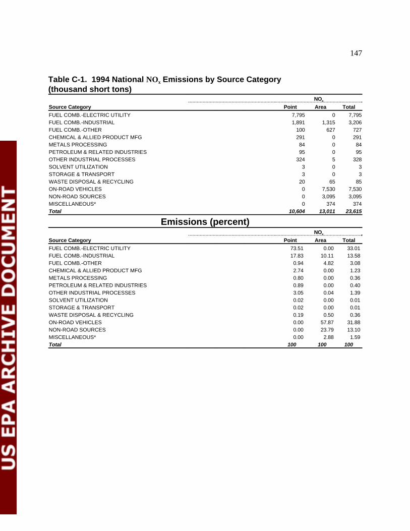
147

Table C-1. 1994 National NO Emissions by Source Categoryx

(thousand short tons)NOx

Source Category Point Area Total

FUEL COMB.-ELECTRIC UTILITY 7,795 0 7,795FUEL COMB.-INDUSTRIAL 1,891 1,315 3,206FUEL COMB.-OTHER 100 627 727CHEMICAL & ALLIED PRODUCT MFG 291 0 291METALS PROCESSING 84 0 84PETROLEUM & RELATED INDUSTRIES 95 0 95OTHER INDUSTRIAL PROCESSES 324 5 328SOLVENT UTILIZATION 3 0 3STORAGE & TRANSPORT 3 0 3WASTE DISPOSAL & RECYCLING 20 65 85ON-ROAD VEHICLES 0 7,530 7,530NON-ROAD SOURCES 0 3,095 3,095MISCELLANEOUS* 0 374 374Total 10,604 13,011 23,615

Emissions (percent)NOx

Source Category Point Area Total

FUEL COMB.-ELECTRIC UTILITY 73.51 0.00 33.01FUEL COMB.-INDUSTRIAL 17.83 10.11 13.58FUEL COMB.-OTHER 0.94 4.82 3.08CHEMICAL & ALLIED PRODUCT MFG 2.74 0.00 1.23METALS PROCESSING 0.80 0.00 0.36PETROLEUM & RELATED INDUSTRIES 0.89 0.00 0.40OTHER INDUSTRIAL PROCESSES 3.05 0.04 1.39SOLVENT UTILIZATION 0.02 0.00 0.01STORAGE & TRANSPORT 0.02 0.00 0.01WASTE DISPOSAL & RECYCLING 0.19 0.50 0.36ON-ROAD VEHICLES 0.00 57.87 31.88NON-ROAD SOURCES 0.00 23.79 13.10MISCELLANEOUS* 0.00 2.88 1.59Total 100 100 100

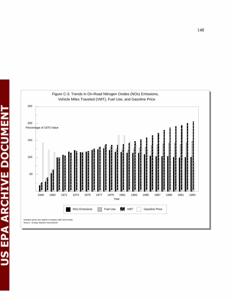
Figure C-3. Trends in On-Road Nitrogen Oxides (NOx) Emissions,Vehicle Miles Traveled (VMT), Fuel Use, and Gasoline Price

1940 1960 1971 1973 1975 1977 1979 1981 1983 1985 1987 1989 1991 1993

50

100

150

200

250

Year

Percentage of 1970 Value

NOx Emissions Fuel Use VMT Gasoline Price

Gasoline prices are stated in constant 1987 price levels.

Source: Energy Statistics Sourcebook

148

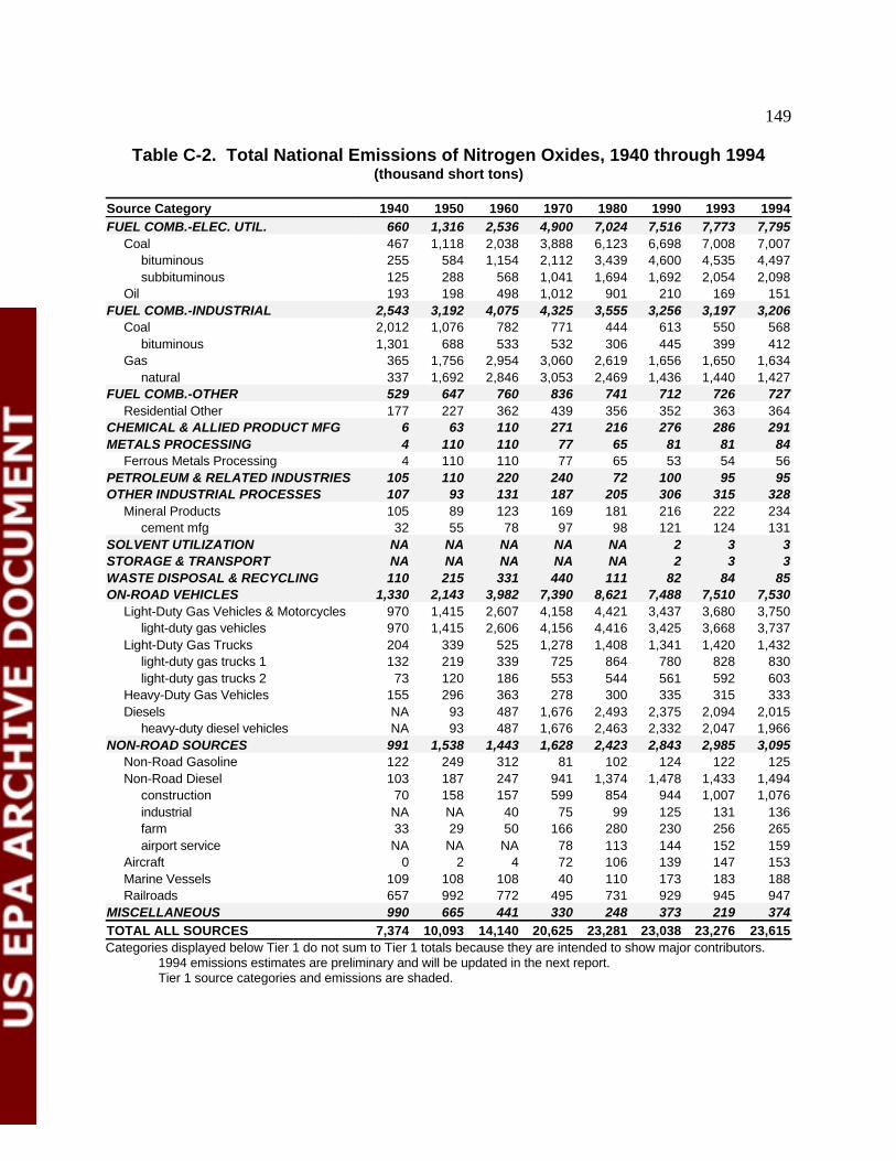
149

Table C-2. Total National Emissions of Nitrogen Oxides, 1940 through 1994(thousand short tons)

Source Category 1940 1950 1960 1970 1980 1990 1993 1994FUEL COMB.-ELEC. UTIL. 660 1,316 2,536 4,900 7,024 7,516 7,773 7,795

Coal 467 1,118 2,038 3,888 6,123 6,698 7,008 7,007bituminous 255 584 1,154 2,112 3,439 4,600 4,535 4,497subbituminous 125 288 568 1,041 1,694 1,692 2,054 2,098

Oil 193 198 498 1,012 901 210 169 151FUEL COMB.-INDUSTRIAL 2,543 3,192 4,075 4,325 3,555 3,256 3,197 3,206

Coal 2,012 1,076 782 771 444 613 550 568bituminous 1,301 688 533 532 306 445 399 412

Gas 365 1,756 2,954 3,060 2,619 1,656 1,650 1,634natural 337 1,692 2,846 3,053 2,469 1,436 1,440 1,427

FUEL COMB.-OTHER 529 647 760 836 741 712 726 727Residential Other 177 227 362 439 356 352 363 364

CHEMICAL & ALLIED PRODUCT MFG 6 63 110 271 216 276 286 291METALS PROCESSING 4 110 110 77 65 81 81 84

Ferrous Metals Processing 4 110 110 77 65 53 54 56PETROLEUM & RELATED INDUSTRIES 105 110 220 240 72 100 95 95OTHER INDUSTRIAL PROCESSES 107 93 131 187 205 306 315 328

Mineral Products 105 89 123 169 181 216 222 234cement mfg 32 55 78 97 98 121 124 131

SOLVENT UTILIZATION NA NA NA NA NA 2 3 3STORAGE & TRANSPORT NA NA NA NA NA 2 3 3WASTE DISPOSAL & RECYCLING 110 215 331 440 111 82 84 85ON-ROAD VEHICLES 1,330 2,143 3,982 7,390 8,621 7,488 7,510 7,530

Light-Duty Gas Vehicles & Motorcycles 970 1,415 2,607 4,158 4,421 3,437 3,680 3,750 light-duty gas vehicles 970 1,415 2,606 4,156 4,416 3,425 3,668 3,737Light-Duty Gas Trucks 204 339 525 1,278 1,408 1,341 1,420 1,432

light-duty gas trucks 1 132 219 339 725 864 780 828 830light-duty gas trucks 2 73 120 186 553 544 561 592 603

Heavy-Duty Gas Vehicles 155 296 363 278 300 335 315 333Diesels NA 93 487 1,676 2,493 2,375 2,094 2,015

heavy-duty diesel vehicles NA 93 487 1,676 2,463 2,332 2,047 1,966NON-ROAD SOURCES 991 1,538 1,443 1,628 2,423 2,843 2,985 3,095

Non-Road Gasoline 122 249 312 81 102 124 122 125Non-Road Diesel 103 187 247 941 1,374 1,478 1,433 1,494

construction 70 158 157 599 854 944 1,007 1,076industrial NA NA 40 75 99 125 131 136farm 33 29 50 166 280 230 256 265airport service NA NA NA 78 113 144 152 159

Aircraft 0 2 4 72 106 139 147 153Marine Vessels 109 108 108 40 110 173 183 188Railroads 657 992 772 495 731 929 945 947

MISCELLANEOUS 990 665 441 330 248 373 219 374TOTAL ALL SOURCES 7,374 10,093 14,140 20,625 23,281 23,038 23,276 23,615Categories displayed below Tier 1 do not sum to Tier 1 totals because they are intended to show major contributors.

1994 emissions estimates are preliminary and will be updated in the next report.Tier 1 source categories and emissions are shaded.

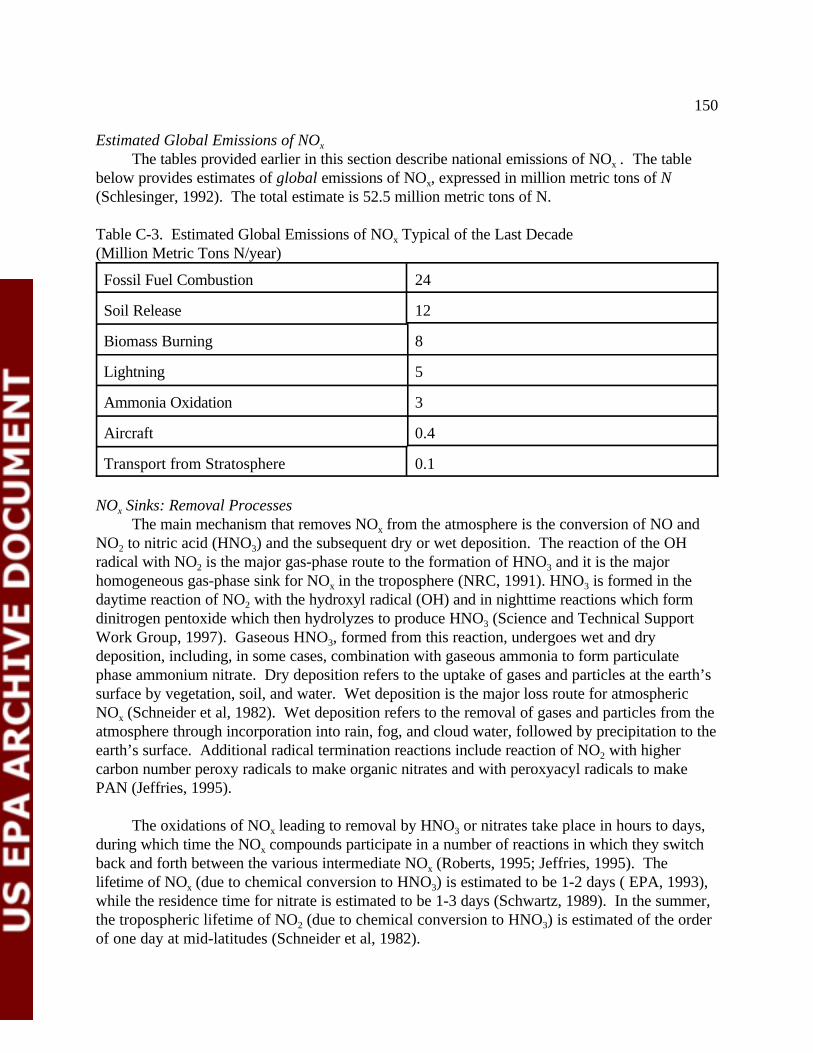
150

Estimated Global Emissions of NOx

The tables provided earlier in this section describe national emissions of NO . The tablex

below provides estimates of global emissions of NO , expressed in million metric tons of Nx

(Schlesinger, 1992). The total estimate is 52.5 million metric tons of N.

Table C-3. Estimated Global Emissions of NO Typical of the Last Decadex

(Million Metric Tons N/year)

Fossil Fuel Combustion 24

Soil Release 12

Biomass Burning 8

Lightning 5

Ammonia Oxidation 3

Aircraft 0.4

Transport from Stratosphere 0.1

NO Sinks: Removal Processes x

The main mechanism that removes NO from the atmosphere is the conversion of NO andx

NO to nitric acid (HNO ) and the subsequent dry or wet deposition. The reaction of the OH2 3

radical with NO is the major gas-phase route to the formation of HNO and it is the major2 3

homogeneous gas-phase sink for NO in the troposphere (NRC, 1991). HNO is formed in thex 3

daytime reaction of NO with the hydroxyl radical (OH) and in nighttime reactions which form2

dinitrogen pentoxide which then hydrolyzes to produce HNO (Science and Technical Support 3

Work Group, 1997). Gaseous HNO , formed from this reaction, undergoes wet and dry3

deposition, including, in some cases, combination with gaseous ammonia to form particulatephase ammonium nitrate. Dry deposition refers to the uptake of gases and particles at the earth’ssurface by vegetation, soil, and water. Wet deposition is the major loss route for atmosphericNO (Schneider et al, 1982). Wet deposition refers to the removal of gases and particles from thex

atmosphere through incorporation into rain, fog, and cloud water, followed by precipitation to theearth’s surface. Additional radical termination reactions include reaction of NO with higher2

carbon number peroxy radicals to make organic nitrates and with peroxyacyl radicals to makePAN (Jeffries, 1995).

The oxidations of NO leading to removal by HNO or nitrates take place in hours to days,x 3

during which time the NO compounds participate in a number of reactions in which they switchx

back and forth between the various intermediate NO (Roberts, 1995; Jeffries, 1995). Thex

lifetime of NO (due to chemical conversion to HNO ) is estimated to be 1-2 days ( EPA, 1993),x 3

while the residence time for nitrate is estimated to be 1-3 days (Schwartz, 1989). In the summer,the tropospheric lifetime of NO (due to chemical conversion to HNO ) is estimated of the order2 3

of one day at mid-latitudes (Schneider et al, 1982).

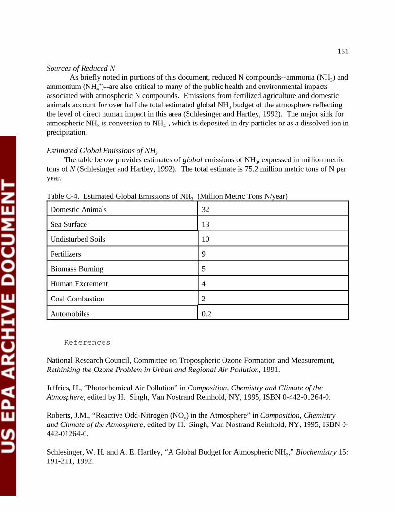
151

Sources of Reduced NAs briefly noted in portions of this document, reduced N compounds--ammonia (NH ) and3

ammonium (NH )--are also critical to many of the public health and environmental impacts4+

associated with atmospheric N compounds. Emissions from fertilized agriculture and domesticanimals account for over half the total estimated global NH budget of the atmosphere reflecting3

the level of direct human impact in this area (Schlesinger and Hartley, 1992). The major sink foratmospheric NH is conversion to NH , which is deposited in dry particles or as a dissolved ion in3 4

+

precipitation.

Estimated Global Emissions of NH3

The table below provides estimates of global emissions of NH , expressed in million metric3

tons of N (Schlesinger and Hartley, 1992). The total estimate is 75.2 million metric tons of N peryear.

Table C-4. Estimated Global Emissions of NH (Million Metric Tons N/year)3

Domestic Animals 32

Sea Surface 13

Undisturbed Soils 10

Fertilizers 9

Biomass Burning 5

Human Excrement 4

Coal Combustion 2

Automobiles 0.2

References

National Research Council, Committee on Tropospheric Ozone Formation and Measurement,Rethinking the Ozone Problem in Urban and Regional Air Pollution, 1991.

Jeffries, H., “Photochemical Air Pollution” in Composition, Chemistry and Climate of theAtmosphere, edited by H. Singh, Van Nostrand Reinhold, NY, 1995, ISBN 0-442-01264-0.

Roberts, J.M., “Reactive Odd-Nitrogen (NO ) in the Atmosphere” in Composition, Chemistryy

and Climate of the Atmosphere, edited by H. Singh, Van Nostrand Reinhold, NY, 1995, ISBN 0-442-01264-0.

Schlesinger, W. H. and A. E. Hartley, “A Global Budget for Atmospheric NH ,” Biochemistry 15:3

191-211, 1992.

152

Schneider, T., and L. Grant, (Editors) Air Pollution by Nitrogen Oxides, 1982, Elsevier ScientificPublishing Company, Amsterdam, The Netherlands, p.252.

Schwartz, S.E., “Acid Deposition: unraveling a regional phenomenon,” Science, 243:753-763,1989.

U.S. Environmental Protection Agency, Air Quality Criteria for Ozone and RelatedPhotochemical Oxidants, external review draft EPA/600/AP-93/004a, 1993.

U.S. Environmental Protection Agency, Office of Air Quality Planning and Standards, NationalAir Pollutant Emissions Trends, 1900-1994, EPA-454/R-95-011, October 1995.

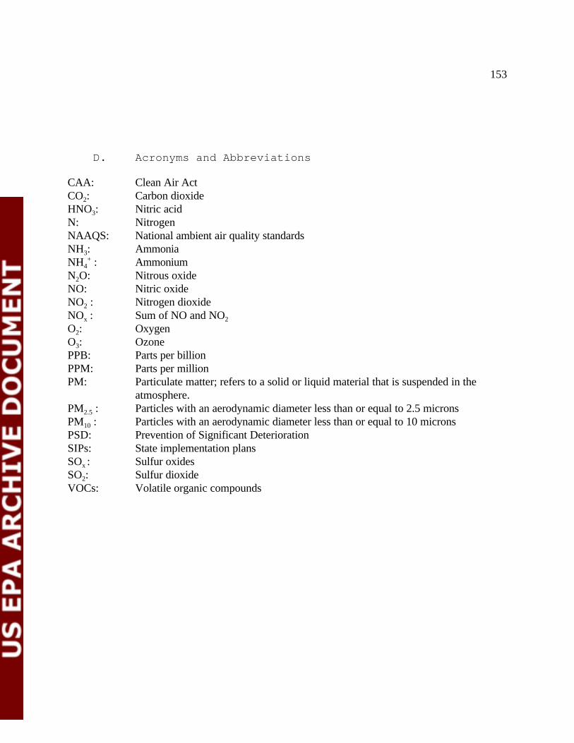
153

D. Acronyms and Abbreviations

CAA: Clean Air ActCO : Carbon dioxide2

HNO : Nitric acid3

N: NitrogenNAAQS: National ambient air quality standardsNH : Ammonia3

NH : Ammonium4+

N O: Nitrous oxide2

NO: Nitric oxideNO : Nitrogen dioxide2

NO : Sum of NO and NOx 2

O : Oxygen2

O : Ozone3

PPB: Parts per billionPPM: Parts per millionPM: Particulate matter; refers to a solid or liquid material that is suspended in the

atmosphere. PM : Particles with an aerodynamic diameter less than or equal to 2.5 microns2.5

PM : Particles with an aerodynamic diameter less than or equal to 10 microns 10

PSD: Prevention of Significant DeteriorationSIPs: State implementation plansSO : Sulfur oxidesx

SO : Sulfur dioxide2

VOCs: Volatile organic compounds