Embed Size (px)
Citation preview

MULTISCALE SIMULATION USING THE GENERALIZED
INTERPOLATION MATERIAL POINT METHOD,
DISCRETE DISLOCATIONS AND
MOLECULAR DYNAMICS
By JIN MA
BACHELOR OF SCIENCE
Wuhan University of Technology Wuhan, China
June, 2000
MASTER OF SCIENCE Oklahoma State University
Stillwater, Oklahoma August, 2002
Submitted to the Faculty of the Graduate College of
Oklahoma State University in partial fulfillment of
the requirements for the Degree of
DOCTOR OF PHILOSOPHY May, 2006

ii
MULTISCALE SIMULATION USING THE GENERALIZED
INTERPOLATION MATERIAL POINT METHOD,
DISCRETE DISLOCATIONS AND
MOLECULAR DYNAMICS
Dean of the Graduate College
Thesis Advisor
Dissertation Approved:
Hongbing Lu, Ranga Komanduri
Jay C. Hanan
Lionel M. Raff
Demirkan Coker
A. Gordon Emslie

iii
© Copyright
By
JIN MA
May 05, 2006

iv
Acknowledgements
I wish to express my most sincere appreciation to my thesis advisor, Dr. Hongbing Lu,
for his intelligent supervision, constructive guidance, inspiration and friendship. Dr. Lu
has also given me very generous financial support. My sincere appreciation extends to
other committee members, Dr. Ranga Komanduri, Dr. Demir Coker and Dr. Lionel Raff,
whose guidance, assistance, encouragement, and friendship are also invaluable. I would
like to thank Dr. Bo Wang, Dr. Jay Hanan, Dr. Samit Roy, Dr. Martin Hagan, Dr. Afshin
J. Ghajar, Dr. C. Eric Price and Dr. J. Keith Good for their long time assistance and
guidance. Moreover, I wish to express my sincere gratitude to those provided suggestions
and assistance for this study: Mr. Gang Huang, Ms. Haowen Yu, Mr. Nitin
Daphalapurkar and Dr. Huiyang Luo.
My research work was supported by a grant from the Air Force Office of Scientific
Research (AFOSR) through a DEPSCoR grant (No. F49620-03-1-0281). I would like to
thank Dr. Craig S. Hartley, and Dr. Jamie Tiley, Program Managers for the Metallic
Materials Program at AFOSR for the support of and interest in this work. Thanks are also
due to Dr. Richard Hornung and Dr. Andy Wissink of the Lawrence Livermore National
Laboratory for providing the code and assistance with the use of SAMRAI, Dr. Scott
Bardenhagen for his introduction to the GIMP algorithm and valuable comments, and Dr.
John A. Nairn for providing the 2D MPM code.
I want to give my special appreciation to my wife, Yang Liu, for her precious suggestions

v
to my study, her encouragement at times of difficulty, her love and understanding
throughout my study. Thanks also go to my parents and my friends for their support and
encouragement.
Finally, I would like to thank the School of Mechanical and Aerospace Engineering for
supporting me during my M.S. and Ph.D. studies.

vi
Table of Contents
Acknowledgements............................................................................................................ iv
Chapter 1 Introduction ........................................................................................................ 1
Chapter 2 Multiscale Simulations Using Generalized Interpolation Material Point (GIMP) Method and SAMRAI Parallel Processing ......................................................................... 4
2.1 Introduction......................................................................................................... 5
2.2 Generalized Interpolation Material Point (GIMP) Method ................................ 9 2.2.1 Contact algorithm in GIMP ...................................................................... 12 2.2.2 Numerical implementation........................................................................ 16
2.3 Parallel Computing Scheme Using GIMP with SAMRAI ............................... 17 2.3.1 SAMRAI ................................................................................................... 17 2.3.2 Spatial and temporal refinements.............................................................. 18 2.3.3 Domain decomposition ............................................................................. 22
2.4 Numerical Examples and Results ..................................................................... 25
2.5 Conclusions....................................................................................................... 34
Chapter 3 Structured Mesh Refinement in GIMP Method for Simulation of Dynamic Problems ........................................................................................................................... 37
3.1 Introduction....................................................................................................... 38
3.2 GIMP................................................................................................................. 40
3.3 Structured Mesh Refinement ............................................................................ 44
3.4 Numerical Simulations...................................................................................... 47 3.4.1 Tracking particle deformation................................................................... 47 3.4.2 Indentation problem.................................................................................. 51 3.4.3 Verification of the displacement boundary condition............................... 54 3.4.4 Stress concentration problem.................................................................... 56 3.4.5 Static stress intensity factor ...................................................................... 58
3.5 Conclusions....................................................................................................... 62
Chapter 4 Simulation of Deformation Mechanism and Failure of Bulk Metallic Glass (BMG) Foam Using the GIMP Method............................................................................ 64
4.1 Introduction....................................................................................................... 65
4.2 Nanoindentation Testing of BMG Foam .......................................................... 70
4.3 Reconstruction of the BMG Foam and Simulation Convergence .................... 72
vii
4.3.1 Reconstruction of the BMG foam for GIMP ............................................ 72 4.3.2 Effect of grid cell size on simulation convergence................................... 74
4.4 Simulation of the BMG Foam in Compression ................................................ 76 4.4.1 Material failure.......................................................................................... 78 4.4.2 Stress flow in the foam ............................................................................. 79 4.4.3 The minimum size of a representative volume element (RVE)................ 81 4.4.4 Simulation of densification ....................................................................... 84
4.5 Conclusions....................................................................................................... 89
Chapter 5 Multiscale Simulation Using GIMP Method and Molecular Dynamics .......... 91
5.1 Introduction....................................................................................................... 92
5.2 GIMP and Refinement ...................................................................................... 96
5.3 MD Simulation and Atomistic Strain ............................................................... 99 5.3.1 Incremental atomic strain........................................................................ 100 5.3.2 Interpolation function.............................................................................. 101 5.3.3 Numerical validation............................................................................... 104
5.4 Coupling of GIMP and MD Simulations ........................................................ 107 5.4.1 Coupling scheme..................................................................................... 107 5.4.2 Parallel processing of the coupled model ............................................... 111
5.5 Numerical Results........................................................................................... 112 5.5.1 Multiscale simulation of mode I crack.................................................... 112 5.5.2 Multiscale simulation of mode II crack .................................................. 117
5.6 Conclusions..................................................................................................... 119
Chapter 6 Multiscale Simulation of Nanoindentation using GIMP, Dislocations Dynamics and Molecular Dynamics ................................................................................................ 122
6.1 Introduction..................................................................................................... 122
6.2 Coupling Scheme between GIMP, DD and MD............................................. 126 6.2.1 Coupling of GIMP and MD .................................................................... 126 6.2.2 Bridging the continuum and atomistic scales with DD .......................... 128 6.2.3 Parallel processing .................................................................................. 130 6.2.4 Contact solver for MD ............................................................................ 133
6.3 Simulation of Nanoindentation ....................................................................... 133
6.4 Conclusions..................................................................................................... 140
Chapter 7 Summary and Future Work ............................................................................ 141
7.1 Summary ......................................................................................................... 141
7.2 Future Work .................................................................................................... 143 7.2.1 Other multiscale problems ...................................................................... 143 7.2.2 Simulation of metal cutting using GIMP................................................ 144

viii
Disclaimer on SAMRAI ................................................................................................. 149
References....................................................................................................................... 150

ix
List of Figures
Fig. 2-1: Illustration of early contact in multi-mesh ......................................................... 13 Fig. 2-2: Schematic of contact algorithm between the rigid indenter and the deformable workpiece.......................................................................................................................... 14 Fig. 2-3: Material points in cells and the weighting function in 2D GIMP...................... 16 Fig. 2-4: Illustration of a hierarchy of three nested grid levels of mesh refinement......... 18 Fig. 2-5: Two neighboring coarse and fine grid levels in 2D GIMP computations.......... 21 Fig. 2-6: Nested multi-level refinement and reduction in the number of cells with number of levels............................................................................................................................. 21 Fig. 2-7: A computational domain of two patches in one grid level................................. 23 Fig. 2-8: Flowchart showing advancement of grid levels recursively starting from the coarsest to the finest level in GIMP.................................................................................. 24 Fig. 2-9: Simulation results of tensile stress contours for a simple tension problem ....... 26 Fig. 2-10: Loading conditions for a simple indentation problem ..................................... 27 Fig. 2-11: GIMP and FEM results of normal stress variation in the Y-direction at different increments .......................................................................................................... 28 Fig. 2-12: Schematic of 2D indentation showing (a) three levels of refinement and (b) the indenter velocity history ................................................................................................... 29 Fig. 2-13: Comparison of normal stresses in Y-direction from FEM and GIMP............. 30 Fig. 2-14: Comparison of shear stresses from FEM and GIMP ....................................... 31 Fig. 2-15: Normal and shear stresses of GIMP simulations with a uniform cell size of 500 nm .............................................................................................................................. 32 Fig. 2-16: Indentation load versus depth curves from FEM and GIMP with different grid sizes................................................................................................................................... 33 Fig. 2-17: Multiscale simulation of nanoindentation with five levels of refinement........ 34 Fig. 3-1: 2D representation of a particle and a grid cell ................................................... 44 Fig. 3-2: Refinement of structured grid with a refinement ratio of two ........................... 45 Fig. 3-3: Effect of influence zone on the weighting functions ......................................... 47 Fig. 3-4: Schematics showing overlaps and gaps that may occur when particle deformation is not tracked ................................................................................................ 48 Fig. 3-5: Simulation showing separation when the particle deformation is tracked by strain.................................................................................................................................. 49 Fig. 3-6: Velocity field of a continuum region (the arrows represent both direction and magnitude) ........................................................................................................................ 50

x
Fig. 3-7: GIMP results with tracking deformation of corners and their comparison with FEM .................................................................................................................................. 51 Fig. 3-8: Two-dimensional indentation simulation........................................................... 52 Fig. 3-9: Comparison of the stress distributions at different levels of refinements in force indentation......................................................................................................................... 53 Fig. 3-10: Comparison of displacement history with FE.................................................. 54 Fig. 3-11: A simple tension problem with displacement boundary conditions ................ 55 Fig. 3-12: Comparisons of the displacement and stress.................................................... 56 Fig. 3-13: A plate with a circular hole subjected to tension ............................................. 56 Fig. 3-14: Normal stress in the X-direction with p = 10 MPa .......................................... 57 Fig. 3-15: Normalized tangential stress along the circumference of the hole .................. 57 Fig. 3-16: Geometry of a double cantilever beam with a crack........................................ 58 Fig. 3-17: Material points and background grid around the crack tip .............................. 60 Fig. 3-18: Computed stress intensity factor as a function of time .................................... 61 Fig. 3-19: Comparison of the stress intensity factor with MPM results .......................... 61 Fig. 3-20: Stress distribution in the beam using three levels of refinements at t = 2.5 ms62 Fig. 4-1: Illustrations of the discretization scheme and intrinsic contact in GIMP .......... 68 Fig. 4-2: High resolution TEM images of (a) crystalline and (b) amorphous structures of a zirconium alloy (Hufnagel (2005)) ................................................................................ 69 Fig. 4-3: Average nanoindentation load-displacement curve with error bars for the BMG foam (Pd43Ni10Cu27P20)..................................................................................................... 71 Fig. 4-4: Schematic of X-ray tomography system............................................................ 72 Fig. 4-5: 3D microtomographic image of a BMG foam ................................................... 73 Fig. 4-6: Stress distribution on a section simulated with the grid size of 3 and 4 times of the voxel size, respectively ............................................................................................... 75 Fig. 4-7: Stress distribution on a section simulated with the grid size to be 1 and 2 times of the voxel size. ............................................................................................................... 76 Fig. 4-8: Experimental setup and nominal stress-strain curve. ......................................... 77 Fig. 4-9: Stress distribution in the overall GIMP model at t = 2.5 μs at location 1. ......... 79 Fig. 4-10: Stress distribution on different sections at t = 2.5 μs. ...................................... 80 Fig. 4-11: Stress distribution on different sections at 8% strain. ...................................... 80 Fig. 4-12: Stress-strain curves of the BMG foam from experiments and simulations using second order interpolation................................................................................................. 82 Fig. 4-13: Stress-strain curves of the BMG foam from experiments, model prediction and simulations using linear interpolation............................................................................... 83 Fig. 4-14: Stress-strain curve from the densification simulation...................................... 85 Fig. 4-15: Comparison of initial and final shapes of the RVE.......................................... 86 Fig. 4-16: Maximum shear stress on section Y-50 at different compressive strains ........ 87 Fig. 4-17: Distribution of zσ stress on section Y-50 at different compressive strains .... 88
xi
Fig. 4-18: Histograms of zε at three compressive strains ................................................ 89 Fig. 5-1: Two neighboring coarse and fine grid levels in 2D GIMP computations.......... 98 Fig. 5-2: 2D representation of a particle and a grid cell ................................................. 103 Fig. 5-3: The generalized interpolation function in 2D .................................................. 104 Fig. 5-4: Two examples to calculate the atomistic strain: (a) Tension (b) Shear ........... 105 Fig. 5-5: Strain histories from different simulations....................................................... 106 Fig. 5-6: Comparison of the normal strain of a surface atom in tension ........................ 106 Fig. 5-7: Illustration of coupled GIMP and MD simulations. The circles represent atoms and squares (smaller than physical size) material points. The material points connect to each other without a gap to represent continuum. .......................................................... 108 Fig. 5-8: Flow chart of the coupling algorithm for one increment ................................. 110 Fig. 5-9: Illustration of three GIMP grid refinements and the domain decomposition for coupling........................................................................................................................... 112 Fig. 5-10: Coupled GIMP/MD simulation of a 2D mode-I edge crack. The dashed lines are the boundaries of the atomistic domain .................................................................... 112 Fig. 5-11: Stress distribution for P = 0.3 eV/Å3.............................................................. 114 Fig. 5-12: Simulation model with an edge crack with P = 0.3 eV/Å3 at t = 208 τ.......... 115 Fig. 5-13: Energies in the model with P = 0.15 eV/Å3 ................................................... 116 Fig. 5-14: Energy release rate P = 0.15 eV/Å3................................................................ 116 Fig. 5-15: Boundary conditions of the mode II crack problem....................................... 117 Fig. 5-16: Comparison of results from pure MD and coupled simulations at t = 11.2 τ 118 Fig. 5-17: Dislocation path at different simulation time................................................. 119 Fig. 6-1: Illustration of coupled GIMP and MD simulations. The circles represent atoms and squares (smaller than physical size) material points. The material points connect to each other without a gap to represent continuum ........................................................... 127 Fig. 6-2: Illustration of the domain decomposition and refinement for the coupling simulation of 2D indentation using GIMP, DD and MD................................................ 131 Fig. 6-3: Flow chart of the coupling algorithm for each increment................................ 132 Fig. 6-4: 2D modeling of an indentation problem with a cylindrical indenter ............... 134 Fig. 6-5: Dislocations and the load-depth curve ............................................................. 134 Fig. 6-6: Comparison of load-depth curves using different contact algorithms ............. 135 Fig. 6-7: Effect of the indentation velocity on the load-depth curve .............................. 136 Fig. 6-8: Effect of the indenter size on the load-depth curve.......................................... 137 Fig. 6-9: Load-depth curves when the ratio between the workpiece size and the indenter radius is constant............................................................................................................. 138 Fig. 6-10: Comparison of the load-depth curves between the coupling and purely MD simulations ...................................................................................................................... 139 Fig. 6-11: Slip bands, discrete dislocations and stress distributions in the model.......... 139 Fig. 7-1: Simulation snap shots of 2D orthogonal metal cutting using GIMP ............... 147
xii
List of Tables
Table 4-1: Nanoindentation results for the BMG foam. ................................................... 71 Table 4-2: Porosity of different volume elements at each location. ................................. 81 Table 7-1: Johnson-Cook material parameters for copper (ABAQUS (2005)).............. 146 Table 7-2: Material properties for copper....................................................................... 146
1
Chapter 1
Introduction
Multiscale simulation is a very important tool to reveal material behavior at different
length and temporal scales through numerical simulations. Despite significant
developments in materials simulation techniques, the goal of predicting reliably the
properties and behaviors of new materials has not yet been achieved. This situation exists
for several reasons that include a lack of full understanding of material behavior at
different scales, absence of scaling laws, computational limitations, and difficulties
associated with experimental measurements of material properties at micro and nano
scales. For example, the information on the mechanical behavior of materials at nano
level is not presently available as input to nanotechnology for the manufacturing of
nanocomponents or microelectro-mechanical systems (MEMS).
Scaling laws governing the mechanical behavior of materials from atomistic (nano), via
mesoplastic (micro), to continuum (macro) scales are very important to numerous
applications, such as the development of a new class of aircraft engine materials, or new
steels for naval battle ships, or new tank armor materials for the army, or numerous
microelectromechanical components for a myriad of applications. Scaling laws are also
important for applications where two length scales of different orders of magnitude are
involved. For example, one is atomistic (nano) and the other mesoplastic (micro) as in
nanoindentation, or, one is mesoplastic (micro) and the other continuum (macro) as in
2
conventional indentation. Appropriate scaling laws may extend the extensive knowledge
accumulated over time on material behavior at the macro (or continuum) level to the
atomistic (or nano) level, via mesoplastic (micro) level.
This work is focused primarily on developing coupling methodologies for continuum and
atomistic simulations. At the continuum level, a new simulation method, the generalized
interpolation material point (GIMP) method (Bardenhagen and Kober (2004)) is used.
GIMP is developed based on the conventional material point method (MPM) (Sulsky et
al. (1995)) with improved simulation stability. In order for GIMP to cover several length
scales, and to couple MD simulations, refinement techniques must be developed.
The thesis is divided into several chapters. Each chapter includes an introduction specific
to that topic and a conclusion of findings. Chapter 2 describes the general theory of
GIMP and multilevel refinement technique at the continuum level based on the
Structured Adaptive Mesh Refinement Application Infrastructure (SAMRAI) (Hornung
and Kohn (2002)). Parallel processing is implemented for GIMP based on SAMRAI and
a contact algorithm is developed for the simulation of nanoindentation problems.
Chapter 3 presents a structured mesh refinement algorithm for GIMP that is smoother
than the method in Chapter 2. The new refinement technique is based on structured mesh
and the refined mesh remains structured. The displacement boundary condition is
explicitly introduced into the discretization of equation of motion in GIMP.
Chapter 4 describes an application of the GIMP method for 3D simulations of bulk
metallic glass (BMG) foams prepared by thermo-plastic expansion. The material points
are created based on the voxels in X-ray tomography so that the microstructure of the
foam is reconstructed exactly in GIMP. The simulation results of uniaxial compression

3
are compared with experimental ones. The densification of foam during compression is
analyzed.
Chapter 5 presents a coupling algorithm for GIMP and MD simulations. A new method
to compute the atomic strain from MD simulation was introduced and validated. The
coupling algorithm enables force, velocity, displacement, and energy compatibility at the
hand-shaking region of the continuum and atomistic domains. Numerical simulations are
performed to validate the coupling algorithm.
The coupling algorithm Chapter 5 is extended to include discrete dislocations in Chapter
6. The discrete dislocation field is coupled with the continuum field using superposition
of boundary conditions. The dislocations in the MD simulation can be detected and
passed into the continuum region and vice versa.
The summary and future works are presented in Chapter 7. The preliminary results of
using GIMP to simulate metal cutting is presented in Chapter 7. This problem involves
issues such as contact, large deformation, material failure, and adaptive mesh refinement.
4
Chapter 2
Multiscale Simulations Using Generalized Interpolation Material Point (GIMP)
Method and SAMRAI Parallel Processing
In the simulation of a wide range of mechanics problems including
impact/contact/penetration and fracture, the material point method (MPM) (Sulsky, Zhou
and Shreyer, (1995)) demonstrated its computational capabilities. To resolve alternating
stress sign and instability problems associated with conventional MPM, Bardenhagen and
Kober (2004) introduced recently the generalized interpolation material point (GIMP)
method and implemented for one-dimensional simulations. In this chapter GIMP has
been extended to 2D and applied to simulate simple tension and indentation problems.
For simulations spanning multiple length scales, based on the continuum mechanics
approach, a parallel GIMP computational method is presented using the Structured
Adaptive Mesh Refinement Application Infrastructure (SAMRAI). SAMRAI is used for
multi-processor distributed memory computations, as a platform for domain
decomposition, and for multi-level refinement of the computational domain. Nested
computational grid levels (with successive spatial and temporal refinements) are used in
GIMP simulations to improve the computational accuracy and to reduce the overall
computational time. The domain of each grid level is divided into multiple rectangular
patches for parallel processing. This domain decomposition embedded in SAMRAI is
very flexible when applied to GIMP. As an example to validate the parallel GIMP

5
computing scheme under SAMRAI parallel computing environment, numerical
simulations with multiple length scales from nanometer to millimeter were conducted on
a 2D nanoindentation problem. A contact algorithm in GIMP has also been developed for
the treatment of contact pair between a rigid indenter and a deformable workpiece.
GIMP results are compared with finite element results on indentation for validation. A
GIMP nanoindentation problem with five levels of refinement was modeled using multi-
processors to demonstrate the potential capability of the parallel GIMP computation.
2.1 Introduction
The material point method (MPM) has demonstrated its capabilities in addressing such
problems as impact, upsetting, penetration, and contact (e.g. Sulsky, Zhou and Schreyer
(1995); Sulsky and Schreyer (1996)). In MPM, two descriptions are used - one based on a
collection of material points (Lagrangian) and the other based on a computational
background grid (Eulerian), as proposed by Sulsky, Zhou and Schreyer (1995). A fixed
structured mesh is generally used in the background throughout the MPM simulations.
The material points are followed throughout the deformation of a solid to provide a
Lagrangian description and the governing field equations are solved at the background
grid nodes so that MPM is not subject to mesh entanglement. Compared to the finite
element method (FEM), MPM takes advantage of both Eulerian and Lagrangian
descriptions and possesses the capability of handling large deformations in a more natural
manner so that mesh lock-up problems present in FEM are avoided. Additionally, for
problems involving contact, MPM provides a naturally non-slip contact algorithm to
avoid the penetration between two bodies based on a common background mesh (Sulsky,
Zhou and Schreyer (1995); Sulsky and Schreyer (1996)). One drawback of the

6
conventional MPM is that when the material points move across the cell boundaries
during deformation, some numerical noise/errors can be generated, Bardenhagen and
Kober (2004). To solve the instability problems associated with the conventional MPM
simulations, Bardenhagen and Kober recently proposed the generalized interpolation
material point method (GIMP) and implemented for one-dimensional simulations.
The present investigation extends the GIMP presented by Bardenhagen-Kober to two-
dimensional simulations and applies it to simple tension and indentation problems.
Furthermore, a refinement technique and a parallel processing scheme are developed so
that the serial GIMP algorithm and code can be extended for parallel computation of
large scale computations based on the continuum mechanics approach.
Parallel processing has been used successfully in numerical analysis using different
methods, such as FEM and boundary element method (BEM) (Mackerle (2003)) and
molecular dynamics (MD) (Kalia and Nakano (1993)). The computational time on
parallel processors can be reduced to a small fraction of the time consumed by a single
processor at the same speed. Parallel processing generally involves issues, such as
domain decomposition/partitioning, load balancing, parallel solver/algorithms, parallel
mesh generation, and multi-grid (Mackerle (2003)). Domain decomposition has been
widely applied in parallel processing in FEM (Hsien (1997)). With partitioning of the
overall computational domain, sequential FEM algorithm usually cannot be used directly
in parallel processing without some modification, primarily due to the coupling of a large
number of simultaneous linear equations. Remeshing is sometimes needed in each sub-
domain. The interfaces of neighboring sub-domains must be meshed identically for
subsequent communications (Mackerle (2003)). These problems are intrinsic to certain

7
numerical methods, such as FEM; however, they can be totally or partially avoided if
other appropriate computational methods are used. For example, the domain
decomposition is more straightforward for structured meshes, and large systems of
coupled equations can be avoided, if explicit time integration is used.
Recently a platform for parallel computation, namely, the structured adaptive mesh
refinement application infrastructure (SAMRAI) (Hornung and Kohn (2002)), has been
developed by the Center for Applied Scientific Computing at the Lawrence Livermore
National Laboratory. SAMRAI has provided interfaces for user-defined data types so that
material points carrying physical variables (mass, displacement, velocity, acceleration,
stress, strain, etc.) can be readily defined. As a result, SAMRAI is very suitable for
handling material points and their physical variables in MPM or its variant, GIMP. In this
investigation SAMRAI is used for parallelizing GIMP. SAMRAI has also provided a
foundation for parallel adaptive mesh refinement (AMR) with the use of either dynamic
or static load balancing (Wissink, Hysom and Hornung (2003)). This function allows
SAMRAI to process both spatial and temporal refinements in areas of interest, typically
with high gradients in some physical variables (e.g., strains), and to use coarse mesh in
the remaining areas. With the appropriate use of fine and coarse meshes in different
regions, multiscale simulations using MPM can provide desired computational accuracy
with reduced costs associated with computer memory and computational time.
Material multiscale simulations span from electronic structure, atomistic scale, crystal
scale, to macro/continuum scale (Horstemeyer, Baskes, Prantil, Philliber and
Vonderheide (2003); Komanduri, Lu, Roy, Wang and Raff (2004)). Appropriate
simulation algorithms can be used at various scales, e.g., ab initio computation for

8
electronic structure, molecular dynamics at the atomistic scale, crystal plasticity or
mesoplasticity at the crystal scale, and continuum mechanics at the macro scale
(Horstemeyer, Baskes, Prantil, Philliber and Vonderheide (2003)). At the continuum
scale, FEM is generally used. Recently, the meshless local Petrov-Galerkin (MLPG)
method (Shen and Atluri (2004a, 2005)) and the continuum/lattice Green function
method (Tewary and Read (2004)) have been used to couple with molecular dynamics
seamlessly. The MLPG method is a simple, less-costly alternative approach to FEM
(Atluri and Shen (2002)). For the purposes of providing the insights into the discrete
atomistic system and coupling with continuum, an equivalent continuum was defined in
the MD region to compute the atomic stress based on the Smoothed Particle
Hydrodynamics (SPH) method (Shen and Atluri (2004b)). The atomic stress tensor
computed using the SPH method is more natural than other atomic stress formulations
because it is in the nonvolume-averaged form and rigorously satisfies the conservation of
linear momentum. Hence, it is applicable to both homogeneous and inhomogeneous
deformations. A tangent stiffness formulation was developed for both MLPG and MD
regions and the displacements of the nodes and atoms are solved in one coupled set of
linear equations. The MLPG/MD coupling has been demonstrated to be capable of
enforcing the local balance equations in the handshaking region between continuum
mechanics and molecular dynamics (Shen and Atluri (2005)).
The simulation using parallel GIMP computing scheme in this investigation will focus on
multiscales, e.g., from nanometer to millimeter, based on the continuum mechanics
approach, namely, 2D GIMP. An example used for validating the simulation at several
length scales at the continuum level is nanoindentation. It involves the contact issue
9
between a rigid indenter and a deformable workpiece. A contact algorithm, which allows
the contact interface to be located in a few computational domains, is introduced in this
study. The contact pressure is determined from solving a set of equations from multiple
processors. Parallel GIMP results on nanoindentation are compared with FEM results
using the ABAQUS/Explicit code. A nanoindentation model with five levels will be used;
this model allows simulation from nanometer to millimeter scales.
2.2 Generalized Interpolation Material Point (GIMP) Method
The governing equations in both conventional material point method (MPM) (Sulsky,
Zhou and Sheryer (1995); Hu and Chen (2003); Bardenhagen (2002)) and generalized
interpolation material point (GIMP) method (Bardenhagen and Kober (2004)) are briefly
summarized in this section. The weak form of the momentum conservation equation in
the conventional MPM is given by
Ω⋅+⋅+Ω∇−=Ω⋅ ∫∫∫∫ ΩΩ∂ΩΩddSdd sbwwcwsaw ss ρρρρ : , (2-1)
where w is the test function, a is the acceleration, and ss, cs and b are the specific stress,
specific traction, and specific body force, respectively. Ω is the current configuration and
∂Ω is the surface with applied traction. The material density, ρ, can be approximated as
the sum of material point masses using a Dirac delta function ∑=
−=pN
p
tpMt
1)(),( xxx δρ ,
where Np is the total number of material points and Mp is the mass of the material point.
Upon discretization of Eq. (2-1) using the shape functions )( tpiN x , the governing
equations at the background grid nodes become (see Sulsky, Zhou and Schreyer (1995))
extint )()( ti
ti
ti
tim ffa += . (2-2)

10
where the lumped mass matrix is given by
∑=
=pN
p
tpip
ti NMm
1
)(x , (2-3)
and the internal and external forces are given by
∑=
∇⋅−=p
tp
N
pi
tspp
ti NM
1
,int)(x
sf , (2-4)
∑∑==
− +−=pp N
p
tpi
tpp
N
p
tpi
tspp
extti NMNhM
11
1, )()()( xbxcf , (2-5)
where h is the thickness of a boundary layer. At each time step, all variables for each
material point, such as mass, velocity, and force are extrapolated to the grid nodes of the
cell in which the material point resides. New nodal momenta are computed and used to
update the physical variables carried by the material points. Thus, material points move
relative to each other to represent deformation in a solid. A spatially fixed background
grid is used throughout the MPM computation. MPM has already demonstrated its
capabilities in solving a number of problems involving impact/contact/penetration. In
case of large deformation, however, numerical noise, or errors have been observed,
especially when material points have just crossed cell boundaries resulting in instability
problems in the MPM simulations (see, e.g., Sulsky, Zhou and Schreyer (1995); Hu and
Chen (2003); Bardenhagen and Kober (2004)). The primary cause for the problem has
been attributed to the discontinuity of the gradient of the shape functions across the cell
boundaries (see, e.g., Hu and Chen (2003); Bardenhagen and Kober (2004)). To resolve
this problem, Bardenhagen and Kober (2004) proposed a generalized interpolation
material point (GIMP) method. In GIMP, the interpolation between node i and material

11
point p is given by the volume averaged weighting function
∫Ω∩Ω
=p
dSV
S ipp
ip xxx )()(1 χ , (2-6)
where Vp is the current volume of the material point, )(xpχ is the characteristic function
of the material point, and Si(x) is the node shape function. The role of the weighting
function is the same as the shape function in conventional MPM. The modified equation
of momentum conservation (Bardenhagen and Kober (2004)) can be written as
∫∑ ∫
∑ ∫∑ ∫
Ω∂Ω∩Ω
Ω∩ΩΩ∩Ω
⋅+⋅
=∇+⋅
xvcxvb
xvσxvp
ddV
m
ddV
p p
pp
ppp
p p
pp
p
pp
δδχ
δχδχ
:&
, (2-7)
where vδ is an admissible velocity field, pp& is the rate of change of the material point
momentum. Eq. (2-7) can be further discretized and solved at the grid nodes,
Bardenhagen and Kober (2004). Herein, the weighting function ipS is C1 continuous
under the spatially fixed background grid. Consequently the noises associated with
material point crossing cell boundaries in the conventional MPM can be minimized.
In this chapter, the GIMP presented by Bardenhagen-Kober is implemented for two-
dimensional simulations. a refinement technique and a parallel processing scheme to
extend the serial GIMP algorithm to code large scale parallel computing have been
developed. The capability of parallel GIMP computing has been demonstrated by
modeling nanoindentation problem. A contact algorithm has been developed to address
the contact problem between the rigid indenter and the deformable workpiece. Next, the
contact algorithm developed in this investigation is described.
12
2.2.1 Contact algorithm in GIMP
Nanoindentation involves a contact pair of a rigid indenter and a deformable workpiece.
The contact interaction between these two surfaces is governed by the Newton’s third law
and Coulomb’s friction law as well as the boundary compatibility condition at the contact
interface (Oden and Pires (1983); Zhong (1993)). While MPM can prevent the
penetration at the interface automatically, it uses a single mesh for the two bodies. At the
contact surface, all components of the variables are interpolated to the nodes from both
bodies using Eqs. (2-3)-(2-5). As a result, MPM using a single mesh tends to induce early
contact in approaching and late separation when two parts move away from each other.
So, MPM cannot model the contact behavior between two parts correctly. Hu and Chen
(2003) proposed a multi-mesh MPM algorithm to release the no-slip constraint inherent
in the MPM using a single mesh. In the multi-mesh MPM, in addition to a common mesh
for all objects, there is an individual mesh for each of the objects under consideration. All
meshes are identical, i.e. nodal locations are the same. The multi-mesh can be generated
by creating multiple nodal fields for each node. Each nodal field corresponds to an object.
In multi-mesh MPM scheme, the nodal masses and forces are mapped from the material
points of each object to its own mesh. The nodal values are transferred to the
corresponding nodes in the common mesh. When the values at a node of the common
background mesh involve contributions from two parts, the contact between two parts
occurs so that this node is defined as an overlapped node. Otherwise, two parts move
independently. This multi-mesh algorithm can handle sliding and separation for the
contact pair. However, in using the multi-mesh for contact problem in GIMP, the
interaction at the overlapped nodes is still activated too early before the actual contact of
13
the material points occurs.
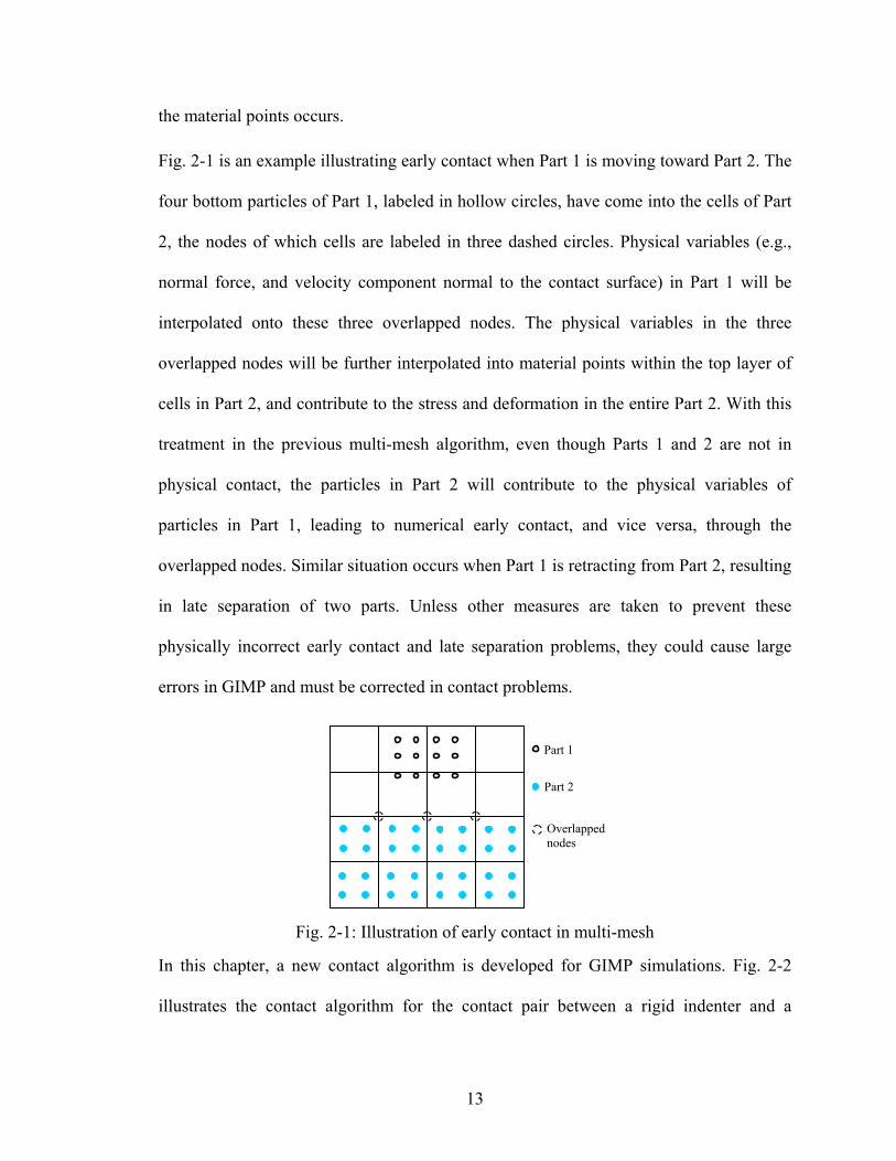
Fig. 2-1 is an example illustrating early contact when Part 1 is moving toward Part 2. The
four bottom particles of Part 1, labeled in hollow circles, have come into the cells of Part
2, the nodes of which cells are labeled in three dashed circles. Physical variables (e.g.,
normal force, and velocity component normal to the contact surface) in Part 1 will be
interpolated onto these three overlapped nodes. The physical variables in the three
overlapped nodes will be further interpolated into material points within the top layer of
cells in Part 2, and contribute to the stress and deformation in the entire Part 2. With this
treatment in the previous multi-mesh algorithm, even though Parts 1 and 2 are not in
physical contact, the particles in Part 2 will contribute to the physical variables of
particles in Part 1, leading to numerical early contact, and vice versa, through the
overlapped nodes. Similar situation occurs when Part 1 is retracting from Part 2, resulting
in late separation of two parts. Unless other measures are taken to prevent these
physically incorrect early contact and late separation problems, they could cause large
errors in GIMP and must be corrected in contact problems.
Fig. 2-1: Illustration of early contact in multi-mesh
In this chapter, a new contact algorithm is developed for GIMP simulations. Fig. 2-2
illustrates the contact algorithm for the contact pair between a rigid indenter and a
Part 1
Part 2
Overlapped nodes

14
deformable workpiece. Although circular points are used in this schematic diagram, it
should be noted that the points are representations of areas occupied by these points,
based on the GIMP algorithm. A frictionless contact is assumed in this investigation. At
the beginning of a time step, a material point is located at point A. At the end of this time
step, the material point moves to B, if there is no contact interaction.
Fig. 2-2: Schematic of contact algorithm between the rigid indenter and the deformable workpiece
To satisfy the displacement compatibility condition, the material point has to be brought
to the indenter surface and kept in contact with the indenter. The contact velocity
correction cpV can be determined based on the rigid surface orientation indicated by its
unit outward normal vector n. The final location of the material point is set to C by a
contact pressure. Hence, the velocity of a material point p under contact can be
determined by
∑∑
∑∑Δ
+Δ+
=
Δ++==
N
iip
i
ci
N
iip
i
ii
N
iip
i
ciii
N
iipip
Sm
tS
mt
Sm
tS
FFp
FFpVV
00
00 )(
, (2-8)
where N is the number of nodes contributing to material point p, ciF is the contact force
on node i, 0ip and 0
iF are the nodal momentum and force without consideration of the
A
C
B
n
D
0pV
cpV
pV
Rigid surface Rigid indenter
Indenter side
Workpiece side
Workpiece
15
contact, respectively. The velocity 0pV of the material point without the consideration of
contact is given by
∑ Δ+=
N
iip
i
iip S
mt00
0 FpV. (2-9)
The contact force ciF on node i is the resultant of the contact pressures on the neighboring
particles, and can be computed in terms of contact pressures using the approach given by
Bardenhagen and Kober (2004), i.e.,
∑ ∫= Ω∂
=Q
q
cqi
ci
q
dsS1
)( PxF , (2-10)
where Q is the total number of material points in contact with the indenter. If the contact
pressure cqP is assumed to be constant in the contact area occupied by material point q,
then, ∑=
=Q
q
cqiq
ci T
1
PF , where ∫Ω∂
=q
dsST iiq )(x . Since cppp VVV += 0 , the contact velocity c
pV for
material point p is given by
∑ ∑Δ=N
i
Q
q
cqiq
i
ipcp T
mSt PV
. (2-11)
Eq. (2-11) can be established for each material point in contact. At each material point
there is an unknown contact pressure cqP . Therefore, the number of unknown pressures,
cqP , is equal to the number of points in contact. In parallel computing, points in contact
might be located in different domains processed by different processors. Consequently, a
parallel solver is needed to solve Eq. (2-11) in this investigation. Since contact can only
occur on the outer surface of an object, Eq. (2-11) is solved analytically under the
physical contact condition 0<⋅nPcq to find the contact pressure at all material points in

16
contact with the indenter. The contact pressure is then extrapolated to the nodes from the
contact material points to update the total nodal forces.
2.2.2 Numerical implementation
Fig. 2-3: Material points in cells and the weighting function in 2D GIMP
Considering the case where initially there are four material points in a cell, the 2D
weighting function is depicted in Fig. 2-3. To compute the weighting function, )(p xχ is
one in the current region occupied by the material point p and zero elsewhere. In this
figure, one node is at the origin and the horizontal axes give material point positions
normalized by the cell size. Fig. 2-3 is based on the same material point characteristic
function and node shape function as in Bardenhagen and Kober (2004). It is noted that
the computation of the weighting function in the deformed state involves some practical
difficulties because the integration boundaries in Eq. (2-7) can be difficult to obtain. To
circumvent this problem, it is assumed that the shape of the region occupied by the four
material points remains rectangular without rotation, so that Eq. (2-6) can be evaluated
analytically. This assumption leads to significant saving in the computational time while
introducing only small errors. Using this assumption, GIMP is extended to 2D
simulations and the results are presented in Section 4.
-1-0.5
00.5
11.5
-1.5 -1 -0.5 0 0.5 1 1.5
0
0.2
0.4
0.6
0.8

17
2.3 Parallel Computing Scheme Using GIMP with SAMRAI
2.3.1 SAMRAI
The Structured Adaptive Mesh Refinement Application Infrastructure (SAMRAI), a
scientific computational package for structured adaptive mesh refinement and parallel
computation, is used with the GIMP for parallel computation of large-scale simulations.
SAMRAI is chosen because of its similarity in grid structure with GIMP. In GIMP, the
computation is usually independent of the background grid mesh so that a structured
spatially-fixed mesh can be used throughout the entire simulation process. This advantage
makes GIMP highly suitable for parallel computation, as the domain decomposition for
structured mesh can be easily performed and no remeshing is required. Thus the
complexity and inefficiency associated with parallel processing can be avoided.
In SAMRAI, the computational domain is defined as a hierarchy of nested grid levels of
mesh refinement (Berger and Oliger (1984)) as shown in Fig. 2-4. Each grid level is
divided into non-overlapping, logically-rectangular patches, each of which is a cluster of
computational cells. Indices are used extensively in SAMRAI to manage grid levels and
patches. For example, patch connectivity is managed by the cell indices. The organization
of the computational mesh into a hierarchy of levels of patches allows data
communication and computation to be expressed in geometrically-intuitive box calculus
operations. Communication patterns for data dependencies among patches can be
computed in parallel without inter-processor communications, since the mesh
configuration is replicated readily across processor memories. Inter-processor
communications, i.e., data communications between patches on the same as well as
neighboring levels, are pre-defined by SAMRAI communication schedules. Problem-

18
specific communication interfaces are also provided by SAMRAI.
SAMRAI supports several data types defined in a patch, such as cell-centered data, node-
centered data, and face-centered data. These data are stored as arrays to allow numerical
subroutines to be separated easily from the implementation of mesh data structures. User-
defined data structures over a patch, which can be accessed through cell index, are
supported by SAMRAI. These characteristics make SAMRAI a very flexible parallel
computing environment for numerous physics applications (Wissink, Hysom, and
Hornung (2003)).
Fig. 2-4: Illustration of a hierarchy of three nested grid levels of mesh refinement
2.3.2 Spatial and temporal refinements
In the application of SAMRAI to large-scale GIMP simulations, the techniques for
refinement, both spatial and temporal, have to be developed to achieve high accuracy in
areas of high stress/strain gradients while reducing the overall computational time by
using coarse mesh in regions of low stress/strain gradients. Since a structured mesh is
used in GIMP, the refinement can be implemented by imposing fine levels of sub-grids at
locations of interest, using the approach adopted by Berger and Oliger (1984) in
SAMRAI. The scheme for the structured grid refinement is illustrated in Fig. 2-4. The
Level 1
Level 2
Level 3

19
cell size ratio, also called the refinement ratio, of two neighboring levels is always an
integer for convenience. The advantage of this refinement technique is that nesting
relationships between different levels can be handled. A material point in GIMP can be
split into several small material points. Tan and Nairn (2004) proposed a criterion to split
material points based on local deformation gradient. If the refinement ratio is two in each
direction, one coarse material point can be split into four material points in the next fine
level in 2D case. However, this splitting technique can become complicated when
conservation of energy and momentum have to be enforced. In this chapter, a more
natural refinement approach is developed to avoid direct splitting and merging processes
by using material points of the same size and mass in overlapped region (called ghost
region) between two neighboring levels.
Fig. 2-5 shows two neighboring coarse and fine grid levels in 2D GIMP computations
with a refinement ratio of two. The thick line represents the physical boundary of the fine
level with four layers of ghost cells. Initially, four material points are assigned to each
cell at the fine level. At the coarse level, the portion overlapped by the fine level is
assigned with 16 material points per cell. Hence, these material points have the same size
and initial positions as those at the fine level. The rest of the coarse level is assigned with
four material points per cell. GIMP provides a natural coupling of the material points
with different sizes at the same grid level. This is because the weighting function depends
on the characteristic size of the material points and cell length and the interpolation
between the nodes and material points is weighed by the mass of the material point. In
GIMP computation, each level is computed independently with the physical variables
communicated through the ghost regions between neighboring levels. Two data exchange

20
processes, namely, refinement and coarsening are used in the communication.
Refinement process passes information from the coarse level to the immediate fine level,
while coarsening process will pass information from fine level to the next coarse level. In
the refinement process, physical variables at the fine material points inside the thick lines
in Fig. 2-5 are copied directly to replace the material points at the coarse level. In the
coarsening process, the physical variables at coarse material points are copied to the
ghost cells of the immediate fine level.
In the refinement, the material points located in the ghost cells at the fine level are
eliminated first, and the material points in the corresponding region of the coarse level
(with the same size as points in the immediate fine level) are copied to ghost cells at the
fine level. In the copying process, if some (small) material points in the coarse level fall
into the interior (inside the square on the right of Fig. 2-5) of the immediate fine level,
these points will not be copied to this fine level, as points in the fine level will be able to
carry over all computations in the interior of the fine level already. In coarsening, the
material points of the coarse level located in the region overlapped by the fine level
(inside the square on the left of Fig. 2-5) are eliminated first, and the material points in
the fine level are then copied to the immediate coarse level. With these
refinement/coarsening operations, the material points can move around freely, including
moving outside the original level in large deformations. To ensure that this coarsening
process can still be performed reliably during deformation, sufficiently wide region of
cells should be assigned with refined material points at the coarse level so that the ghost
cells of the fine level always stay within the region with fine material points on the coarse
level. At the coarse level, the interior cells covered by the fine level do not participate in

21
the computation and there are no material points inside (see Fig. 2-5).
Fig. 2-5: Two neighboring coarse and fine grid levels in 2D GIMP computations
Fig. 2-6: Nested multi-level refinement and reduction in the number of cells with number of levels
The refinement techniques can be applied for multiple times at the regions of interest,
such as the stress concentration regions. A fixed refinement ratio of two between two
neighboring levels is very effective in reducing the total number of computational cells.
Fig. 5 shows nested multi-level refinement and its corresponding relation between the
total number of cells and the number of grid levels. The cell percentage represents the
ratio of the total number of cells with multi-level refinement mesh to the total number of
cells with one-level finest mesh. If each fine level occupies one quarter of the
neighboring coarser level, as shown in Fig. 2-6 (a), the cell percentage as a function of
Coarse Fine
Level 1
Level 2
3
(b)
0
20
40
60
80
100
1 2 3 4 5 6 7Number of levels
Cel
l per
cent
age
(%)
(a)
22
the number of grid levels can be calculated, as shown in Fig. 2-6 (b). For example, when
totally four levels of successive refinements are used the total number of cells is about
8% of that of one uniform fine mesh. A reduction in the number of computational cells
leads to a reduction in the number of material points. Hence, the total amount of
computational time can be reduced significantly. However, refinement and coarsening
communications will cost additional computational time, as will be discussed in Section 4.
Another advantage of the multi-level refinement is that it allows for temporal refinement.
Since the computation at each grid level is conducted independently, different time step
increments can be used for computation at different levels. For example, a smaller time
step increment can be used for the fine level to improve computational accuracy, while a
larger time step increment can be used for the coarse level. Since the refinement ratio is
an integer, the time step increment ratio should also be an integer for convenience in the
computation and data communication/synchronization. For example, in Fig. 2-5, when
the refinement ratios in both directions are fixed at two, the time step increment ratio
should be set to two as well. As a result, two time step computations are performed at the
fine level, and results are passed over to the immediate coarse level to couple with the
results at the coarse level.
2.3.3 Domain decomposition
GIMP uses structured mesh, consistent with SAMRAI, so that domain decomposition is
straightforward and no remeshing, in general, is necessary. Fig. 2-7 (a) shows a two-
dimensional computational domain decomposed into two patches separated by a
horizontal dash line. The elliptical solid object with different boundary conditions applied
at different regions is inside this domain/grid. After discretization, there are a certain

23
number of material points and part of the boundary in a patch, which will be computed
individually. It may be noted that patch boundary does not have to coincide with the
boundary of the material continuum. The patch boundary is always chosen to be larger
than the region occupied by the material continuum so that there is extra space for the
material to deform. This will not cause any additional computational burden as the GIMP
computation is only carried out on material points inside the patch. Each patch can be
processed by a single processor and the convenience in creating patches will provide
great flexibility in parallel processing.
Fig. 2-7: A computational domain of two patches in one grid level
Communication between two neighboring patches is realized through information sharing
in the region overlapped by the two patches. The overlapped regions are also called
“ghost” regions, as shown in Fig. 2-7 (b). The ghost cells are denoted by dash lines. For
ease of visualization, only the ghost cells overlapped by the other patch are shown and
the ghost cells along the other three sides of a patch are not shown. On one grid level,
patches can communicate with each other by simply copying data from one patch to
another at the same computation time (Fig. 2-7 (b)). Using the material point information
from the previous time step, and the physical boundary conditions, each patch is ready to
advance one more time step. At this time, the material point information in the outermost
Patch 2
Patch 1
Ghost of patch 1 Copy from patch 2
Ghost of patch 2 Copy from patch 1
(a) (b)
24
layer of the ghost cells becomes inaccurate. For instance, one outermost grid node in
patch one, marked by the circle, obtains information from eight material points before
advancing to the next step. After advancing, it extrapolates to eight material points.
However, in patch two, the grid node at the same location obtains information from
sixteen surrounding material points. It extrapolates to these sixteen material points after
advancing. Typically, after each step, the material points in the next inner layer in the
ghost region become inaccurate as well.
Ghost cells and material points are attached to each patch to ensure accuracy of the
interior. Each patch can be computed independently for one GIMP step since the
momentum conservation equation is solved at each node and there are no coupled
equations to solve. No data exchange is necessary during the GIMP step. Therefore,
different patches can be assigned to different processors for parallel processing. After one
GIMP step, the data in the ghost cells will be updated.
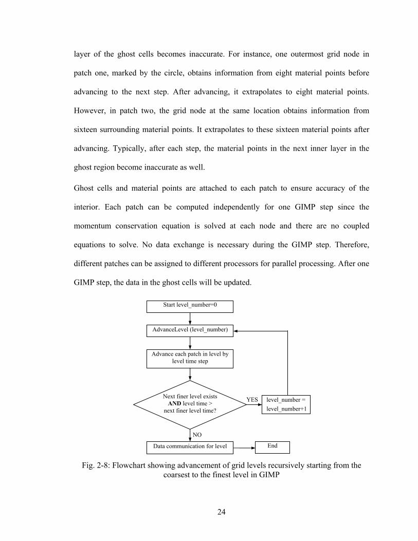
Fig. 2-8: Flowchart showing advancement of grid levels recursively starting from the coarsest to the finest level in GIMP
AdvanceLevel (level_number)
Advance each patch in level by level time step
Start level_number=0
Next finer level exists AND level time >
next finer level time?
level_number = level_number+1
Data communication for level
YES
NO
End

25
Copying material points to ghost cells involves data exchange between processors, which
costs additional time. The more the number layers of ghost cells, the longer the time
needed for communication, but communication can be performed less frequently. A
minimum of two layers of ghost cells are necessary to ensure that computation at the
material points inside a patch is always correct. If three levels of ghost cells are chosen,
the communication can be performed after every two increments of each patch.
With these refinements and domain decomposition schemes for GIMP, it is possible to
implement GIMP into the SAMRAI platform. In this study, the refinement ratio is chosen
as two. Four layers of ghost cells are augmented to a patch such that data
communications, including both data exchange on the same level and between
neighboring levels, are performed every two time-steps for each fine grid level. This is
critical because data exchange between levels has to be performed when the two levels
are synchronized. Fig. 2-8 shows the flowchart advancing all grid levels recursively
starting from the coarsest level for one coarsest time step. It may be noted that the
sequential GIMP algorithm can be used to advance each patch without modification.
2.4 Numerical Examples and Results
A Beowulf Linux cluster of 8 identical PCs were used in the simulations. Each PC has a
Pentium 4 processor with a 2.4 GHz CPU, 512 MB RAM except that the master node has
a memory of 1 GB. A gigabit switch is used to connect the network.
Two examples are used for validation of the 2D parallel GIMP computing under
SAMRAI platform. The first example is simple tension of polycrystalline silicon under
plane strain conditions. The material is assumed to be homogeneous, isotropic, and linear
elastic. The Young’s modulus is 170 GPa and the Poisson’s ratio is 0.18. One end is

26
constrained along the X- direction while a normal traction is ramped up on the other end.
The size of the tensile model is 0.06 mm × 0.04 mm. The length of a square grid cell is
0.002 mm and the time step is 5×10⁴ ps. For verification, the same problem was
simulated using both conventional MPM and FEM (ABAQUS/Explicit). Fig. 2-9 shows
GIMP, MPM and FEM simulation results of normal stresses in the X-direction at
different increments from a simple tension problem. The simulation using the
conventional MPM in Fig. 2-9 (a) shows material separation close to the free end with
severe numerical instability after 275 increments. Fig. 2-9 (b) and (c) show the normal
stress distribution in the tensile direction and deformation after 500 increments from
FEM and GIMP. It may be noted that FEM results show a stress contour plot on the
deformed mesh while the GIMP results show a discrete scattered plot of material points.
These two results are in good agreement with the difference in the maximum value being
less than 10%.
Fig. 2-9: Simulation results of tensile stress contours for a simple tension problem
(c) FEM
(a) Conventional MPM (b) GIMP
27
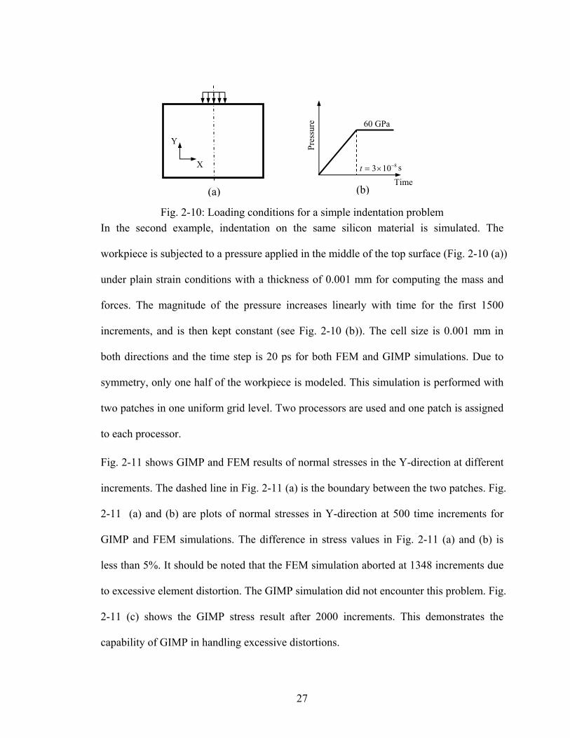
Fig. 2-10: Loading conditions for a simple indentation problem In the second example, indentation on the same silicon material is simulated. The
workpiece is subjected to a pressure applied in the middle of the top surface (Fig. 2-10 (a))
under plain strain conditions with a thickness of 0.001 mm for computing the mass and
forces. The magnitude of the pressure increases linearly with time for the first 1500
increments, and is then kept constant (see Fig. 2-10 (b)). The cell size is 0.001 mm in
both directions and the time step is 20 ps for both FEM and GIMP simulations. Due to
symmetry, only one half of the workpiece is modeled. This simulation is performed with
two patches in one uniform grid level. Two processors are used and one patch is assigned
to each processor.
Fig. 2-11 shows GIMP and FEM results of normal stresses in the Y-direction at different
increments. The dashed line in Fig. 2-11 (a) is the boundary between the two patches. Fig.
2-11 (a) and (b) are plots of normal stresses in Y-direction at 500 time increments for
GIMP and FEM simulations. The difference in stress values in Fig. 2-11 (a) and (b) is
less than 5%. It should be noted that the FEM simulation aborted at 1348 increments due
to excessive element distortion. The GIMP simulation did not encounter this problem. Fig.
2-11 (c) shows the GIMP stress result after 2000 increments. This demonstrates the
capability of GIMP in handling excessive distortions.
X
Y
(a) (b)Time
Pres
sure
8103 −×=t s
60 GPa

28
Fig. 2-11: GIMP and FEM results of normal stress variation in the Y-direction at
different increments
In order to validate the multi-level refinement algorithm and parallel communication, as
well as the proposed contact algorithm, a simulation of nanoindentation with a wedge
indenter was conducted under 2D plane strain conditions. The workpiece is aluminum
and the indenter is assumed to be rigid. Fig. 11 shows the indentation model. The area
below the indenter where high stress gradients are expected is refined, as shown in Fig.
2-12 (a). A prescribed velocity was applied on the indenter, as shown in Fig. 2-12 (b).
(c) GIMP at 2000 increments
(a) GIMP at 500 increments (b) FEM at 500 increments

29
The work piece dimensions are 60 µm × 40 µm. It is fixed in the Y-direction at the
bottom. Only half of the model is simulated because of symmetry. The cell sizes are 500
nm, 250 nm and 125 nm for levels 1, 2 and 3, respectively. Each level is divided into four
patches with approximately the same size. The maximum indentation depth in the
simulation is about 450 nm. The dotted lines in Fig. 2-12 (a) illustrate the four patches in
level 1. For comparison, an explicit FEM simulation (using ABAQUS/Explicit) was
carried out under the same conditions. The FEM element size is uniform and is the same
size as the finest GIMP background grid size. In this example, the maximum indentation
depth (450 nm) is relatively small compared to the finest cell size, so that FEM
simulation has not encountered excessive mesh distortion.
Fig. 2-12: Schematic of 2D indentation showing (a) three levels of refinement and (b) the indenter velocity history
Fig. 2-13 shows a comparison of contours of normal stresses in the Y-direction at the
maximum depth for both FEM and parallel GIMP simulations. The axis of symmetry of
the workpiece is located at X = 0.03 mm. For FEM, the plot is the contour of nodal
stresses with deformed positions, and for GIMP, it is a discrete scattered plot of stress at
deformed material points. The area below the indenter with high stress gradients is
refined as shown in Fig. 2-12 (a) for parallel GIMP computation. The borders of grid
levels 2 and 3 can barely be seen in Fig. 2-13 (b) due to the use of high material point
(a) (b)
Time
V
20 m/s
V
Level 1
Level 2
3
X
Y

30
density. Fig. 2-14 is a close-up view of shear stresses in which the three grid levels are
shown. Results show that the normal and shear stresses from both parallel GIMP and
FEM simulations agree very well. The difference of the normal stresses in the Y-direction
for the material point in contact with the indenter tip and the stress of the FEM node at
the same location is 4.4%. It may be noted that some non-smoothness in the GIMP
stresses around the level boarders can be seen. This non-smoothness is caused by the
refinement and coarsening and the error associated with this is negligible for these
simulations.
Fig. 2-13: Comparison of normal stresses in Y-direction from FEM and GIMP
GIMP simulations using a uniform cell size of 500 nm and 125 nm were performed under
the same conditions as in Fig. 2-12 to further verify the refinement/coarsening algorithm.
Fig. 2-15 shows normal stresses in the Y-direction and shear stresses in GIMP
simulations using 500 nm uniform cells. In this case the material points in contact with
the indenter are 16 times (4 times in each direction) larger than those with two levels of
refinements. In general, the stress magnitudes agree with those in Fig. 2-13 and Fig. 2-14.
Fig. 2-16 (a) shows indentation load versus depth curves from FEM and GIMP with
(b) GIMP (a) FEM

31
different grid sizes. From GIMP computations, the load versus depth curves with three
levels of refinement agree very well with the results from a uniform finest mesh. The load
versus depth curve from the FEM simulation with a uniform cell size of 125 nm under the
same boundary conditions is plotted for comparison. It can be seen from Fig. 2-16 (a) that
the trend of the load versus depth plots from FEM and GIMP simulations are similar.
The difference in indentation load at the end of loading, which corresponds to 450 nm of
indentation depth, is 5.9% between FEM and GIMP with 3 grid levels. When the depth is
less than 100 nm, there is only one material point in contact with the rigid indenter. The
assumption of constant pressure causes large differences under this circumstance.
However, if the GIMP cell size is further refined to 62.5 nm and the size of the material
point is 31.25 nm, the difference between GIMP and FEM becomes smaller, as can be
seen in Fig. 2-16 (b).
Fig. 2-14: Comparison of shear stresses from FEM and GIMP
Other simulations were conducted for the same problem with three levels of refinement
using different number of processors to test the efficiency of parallel computing. The
number of patches at each level is the same as the number of processors and the size of
(b) GIMP (a) FEM

32
each patch is approximately the same. The resultant stress distribution and indentation
load versus depth plots are the same as the previous results. The average time per
computational step is 7.14 s when one processor is used and is reduced to 4.26, 3.40, 2.18
s, respectively when two, three, and four processors are used. When four processors are
used, the CPU time per step is only 30.5% of that of one processor. This gives a speed-up
by a factor of 3.28. In the ideal case without communication overhead, the speed-up
would be 4. The reduction in speed-up from the ideal number is because of the time
involved in data communication between processors. It has been observed that the
refinement and coarsening algorithm consume most of the communication time.
Moreover, in refinement and coarsening, most of the time is taken to search for the
corresponding material point in another grid level. This portion of the computational time
can be reduced, if improved searching algorithm or more optimized algorithm for the
storage of material points can be implemented.
Fig. 2-15: Normal and shear stresses of GIMP simulations with a uniform cell size of 500 nm
The manual refinement for the indentation problem is adequate since the region of high
(b) Shear Stress (a) Normal Stress

33
stress gradient is known to occur below the indenter. The finest level covers the indenter
and part of the specimen. With the same initial condition, the results at the finest level is
identical to the results in the same area if a uniform fine mesh is used for the entire
domain that requires much longer computational time. The computational load of each
processor is balanced statically by assigning approximately the same number of material
points to each processor. Dynamic load balance is supported by SAMRAI and can
potentially improve the efficiency of the simulation.
Fig. 2-16: Indentation load versus depth curves from FEM and GIMP with different grid sizes
To demonstrate the capability of the algorithm developed in this investigation for
multiscale simulation, an indentation model with multiple length scales is simulated with
eight processors. The dimensions of the workpiece are 0.25 mm × 0.125 mm. Initially,
the velocity of the indenter increases from 0 to 150 m/s linearly with time and is then
kept constant. Five successive levels of refinement are used in this simulation. The
smallest material point represents an area of 64 nm × 64 nm, and the largest material
point covers an area of 1 μm × 1 μm. Each level is divided into 8 equal-sized patches for
best load balance. Since the contact surface can evolve into several patches, a parallel
0
1
2
3
4
5
6
0 100 200 300 400 500
Depth (nm)
Load
(mN
)
GIMPM-coarse (500 nm)
GIMPM-fine (125 nm)
GIMPM-3 levelsFEM-fine (125 nm)
0
0.5
1
1.5
2
2.5
0 40 80 120 160
Depth (nm)
Load
(mN
)
GIMPM-500 nm
GIMPM-125 nm
GIMPM-62.5 nmFEM-62.5 nm
(a) (b)

34
solver is implemented to solve Eq. (2-11) to find the contact pressure based on the
Portable, Extensible Toolkit for Scientific Computation (PETSc). An aluminum
workpiece is chosen with the Young’s modulus and Poisson’s ratio of 70 GPa and
0.33, respectively. The maximum indentation depth was 9.8 μm in this simulation (i.e.,
153 times the size of the finest material point). It took nine hours to simulate this problem
with eight processors. Fig. 2-17 (a) gives the normal stress distributions and Fig. 2-17 (b)
shows normal stress distribution for the finest two levels. The relative large deformation
in this multiscale nanoindentation problem could not be handled by FEM due to
excessive distortion in the FEM mesh. However, the parallel GIMP code was able to
complete the entire loading/unloading processes without any difficulty. This example
shows clearly the advantage of GIMP for multiscale simulations over FEM.
Fig. 2-17: Multiscale simulation of nanoindentation with five levels of refinement
2.5 Conclusions
The following are specific conclusions based on the results of this investigation:
A 2D generalized interpolation material point (GIMP) method has been implemented to
address problems, such as particle flying-off and alternating stress sign associated with
(a) (b)
35
conventional MPM in case of relatively large deformation.
To conduct multiple length scale simulations, a parallel computing scheme has been
presented using GIMP under SAMRAI parallel computing environment in which multi-
level grids are used for spatial and temporal refinements.
A refinement/coarsening algorithm, based on material points of GIMP in two grid levels,
has been developed for communication between neighboring grid levels of different
refinements. With increase in the refinement levels, as well as decrease in the time step
increments, the computational accuracy is greatly improved in the region of interest while
the overall computational time is reduced. The computation at each grid level is
performed recursively to ensure that the refinement and coarsening are performed when
the two neighboring levels are synchronized.
2D MPM and GIMP were applied to simple tension and indentation problems to validate
the GIMP algorithm. GIMP results agree very well with FEM results for these two
examples provided that the deformations are small. The noise and instability problems
present in conventional MPM are not observed in the GIMP simulations.
As the deformation is increased, GIMP continued to execute while FEM aborted due to
element distortion. Also GIMP results are stable. Thus GIMP is able to handle relatively
large deformation problems.
For the nanoindentation problem, a GIMP algorithm for the contact between a rigid
indenter and a deformable workpiece was developed. A reasonably good agreement
between GIMP and FEM results was reached, validating the contact algorithm presented
in this investigation.
Another nanoindentation example with multiple length scales from a few nanometers to

36
sub-millimeters was simulated and numerical results validated the parallel GIMP
computing with the use of SAMRAI.

37
Chapter 3
Structured Mesh Refinement in GIMP Method for Simulation of Dynamic Problems
The generalized interpolation material point (GIMP) method, recently developed using a
C1 continuous weighting function, has solved the numerical noise problem associated
with material points just crossing the cell borders, so that it is suitable for simulation of
relatively large deformation problems. However, this method typically uses a uniform
mesh in computation when one level of material points is used, thus limiting its
effectiveness in dealing with structures involving areas of high stress gradients. In this
chapter, a spatial refinement scheme of the structured grid for GIMP is presented for
simulations with highly localized stress gradients. A uniform structured background grid
is used in each refinement zone for interpolation in GIMP for ease of generating and
duplicating structured grid in parallel processing.
The concept of influence zone for the background node and transitional node is
introduced for the mesh size transition. The grid shape function for the transitional node
is modified accordingly, whereas the computation of the weighting function in GIMP
remains the same. Two other issues are also addressed to improve the GIMP method. The
displacement boundary conditions are introduced into the discretization of the momentum
conservation equation in GIMP, and a method is implemented to track the deformation of
the material particles by tracking the position of the particle corners to resolve the
problem of artificial separation of material particles in GIMP simulations. Numerical

38
simulations of several problems, such as tension, indentation, stress concentration and
stress distribution near a crack (mode I crack problem) are presented to validate this
refinement scheme.
3.1 Introduction
The material point method (MPM) uses a collection of material points, mathematically
represented by Dirac delta functions to represent a material continuum (Sulsky, Zhou,
and Schreyer (1995); Hu and Chen (2003); Guilkey and Weiss (2003)). A spatially fixed
background grid, and interpolation between grid nodes and material points are introduced
to track physical variables carried by the material points in the Lagrangian description.
Field equations are solved on the background grid in the Eulerian description. Physical
variables are interpolated from the solutions on the background grids to material points
back and forth for solution and convection of physical variables. In general, the
isoparametric shape functions, same as those used in the finite element method (FEM),
are used. As the MPM simulation is independent of the background grid, a structured grid
is usually employed for purposes of simplicity. The movement of the material points
represents the deformation of the continuum. MPM has been demonstrated to be capable
of handling large deformations in a natural way (Sulsky, Zhou, and Schreyer (1995)).
However, primarily due to the discontinuity of the gradient of the interpolation function
at the borders of the neighboring cells, artificial noise can be introduced when the
material points move just across the grid cell boundaries, leading to simulation instability
for MPM. The generalized interpolation material point (GIMP) method, introduced by
Bardenhagen and Kober (2004) can resolve this problem. In GIMP a C1 continuous
interpolation function is used and each material point/particle occupies a region. GIMP
39
has been demonstrated to be stable and capable of handling relatively large deformations
(Ma, Lu, Wang, Roy, Hornung, Wissink, and Komanduri (2005)).
The current MPM typically uses a uniform background mesh for solving the field
equations. However, this is not efficient when stress gradients are high such as stress
concentrations in a plate with a hole, or the stress field of a workpiece under indentation.
In contrast, transitional mesh is effective in solving problems involving rapidly varying
stress in an area. Wang, Karuppiah, Lu, Roy, and Komanduri (2005) have presented a
method using an irregular background mesh to deal with problems involving rapidly
varying stress, such as stress field near a crack. However, this approach does not use
regular structured background mesh so that mesh generation encounters the same
difficulty as FEM, and leads to the loss of some advantage of MPM on the ease of
generating mesh for a complex problem.
The use of structured grid in GIMP has facilitated the implementation of GIMP in
parallel processing. A refinement scheme based on splitting and merging material
particles was proposed by Tan and Nairn (2002). Recently, a multilevel refinement
algorithm has been developed for parallel processing using the structured adaptive mesh
refinement application infrastructure (SAMRAI) (Hornung and Kohn (2002); Ma, Lu,
Wang, Roy, Hornung, Wissink and Komanduri (2005)). The computational domain is
divided into multiple nested levels of refinement. Each grid level is uniform but has a
different cell size. Smaller material particles and smaller cell sizes are used in each finer
level. Two neighboring levels are connected by overlapped material particles of the same
size and data communication between levels is performed at predefined intervals.
However, the refinement through material particles requires extra communication and
40
simulation time. In this chapter, a refinement for GIMP based on the transitional grid
nodes is developed. This refinement is natural and does not involve extra simulation time.
Moreover, the refined grid remains uniformly structured in each refinement region.
While the problem associated with artificial noise has been resolved with the use of
GIMP method, it has been observed recently that material separation could occur if the
deformation of the material particles was not tracked (Guilkey (2005)). Tracking the
deformation of material particles properly in GIMP is necessary especially when the
material particles are stretched. In this chapter, an approach is developed for tracking the
particle deformation to resolve material point separation problem. This chapter focuses
on the refinement scheme for structured grid. Several numerical problems, such as
tension, indentation, stress concentration and stress distribution near a crack (mode I
crack problem) were simulated to verify this refinement algorithm, as well as to
demonstrate the effectiveness of tracking particle deformations.
3.2 GIMP
For the purpose of completeness, the basic equations in GIMP (Bardenhagen and Kober
(2004)) are summarized here. In dynamic simulations, the mass and momentum
conservation equations are given by
0=⋅∇+ vρρdtd
, and (3-1)
bσa +⋅∇=ρ in Ω , (3-2)
where ρ is the material density, a is the acceleration, σ and b are the Cauchy stress and
body force density, respectively. The displacement and traction boundary conditions are
given as
41
uu = on uΩ∂ , (3-3)
ττ = on τΩ∂ , (3-4)
where ,Ω∂⊂Ω∂ u Ω∂⊂Ω∂ τand .0=Ω∂∩Ω∂ τu In variational form, the momentum
conservation equation can be written as
∫∫∫∫Ω∂ΩΩΩ
⋅−−⋅+⋅∇=⋅u
dddd xvuuxvbxvσxva δαδδδρ )( , (3-5)
where vδ is an admissible velocity field, α is a penalty parameter introduced herein to
impose the essential boundary conditions and 1>>α (Atluri and Zhu (1998); Atluri and
Zhu (2000)). Applying the chain rule, vσvσvσ δδδ ∇−⋅∇=⋅⋅∇ :)()( , and the
divergence theorem, Eq. (3-5) can be written as
∫∫
∫∫∫∫
Ω∂Ω∂
Ω∂ΩΩΩ
⋅−−⋅+
⋅+⋅=∇+⋅
uu
dSdS
dSddd
u vuuvτ
vτxvbxvσxva
δαδ
δδδδρτ
)(
:
, (3-6)
where uτ is the resultant traction due to the displacement boundary condition on uΩ∂ . In
GIMP, the domain Ω is discretized into a collection of material particles, with pΩ as the
domain of particle p. The physical quantities, such as the mass, stress and momentum can
be defined for each particle. For example, the momentum for particle p can be expressed
as ∫Ω
=p
dpp xxxvxp )()()( χρ , where )( xv is the velocity and )(p xχ is the particle
characteristic function. The momentum conservation equation can be discretized as
∑ ∫∑ ∫∑ ∫
∑ ∫∑ ∫∑ ∫
Ω∩Ω∂Ω∩Ω∂Ω∩Ω∂
Ω∩ΩΩ∩ΩΩ∩Ω
⋅−⋅+⋅+
⋅=∇+⋅
ppu
p
p p
pp
ppp
p p
pp
pupup
ppp
dSdSd
dV
mdd
V
vu-uvτxvτ
xvbxvσxvp
δαδδ
δχ
δχδχ
τ
)(
:&
. (3-7)
42
where ∫Ω∩Ω
=p
dV pp xx)(χ is the particle volume. Introducing a background grid and the
grid shape function )(xiS that satisfies partition of unity 1)( =∑i
iS x , the admissible
velocity field can be represented by the grid nodal data as ∑=i
ii S )(xvv δδ . Without the
loss of generality, take u in Eq. (3-7) to be the displacement of the boundary particles at
the current time step and upu nστ = where un is the unit outward normal to uΩ∂ . The
momentum conservation, Eq. (3-7), can eventually be written for each node i as
uii
biii ffffp +++= τint& , (3-8)
where the time rate change of nodal momentum ,/∑ Δ=p
pipi tS pp& the nodal internal
force vector ,int ∑ ∇⋅−=p
pippi VSσf the nodal body force vector ∑=p
ippbi Sm bf and the
nodal traction force vector ∑ ∫Ω∩Ω∂
=p
ii
p
dSSτ
τ )(xτf . uif is the force vector induced by the
essential boundary condition given by
∑ ∫∑ ∫Ω∩Ω∂Ω∩Ω∂
−=p
ipp
iupui
pupu
dSSdSS )()()( xu-uxnσf α . (3-9)
ipS is weighting function between particle p and node i given as
∫Ω∩Ω
=p
dSV
S ipp
ip xxx )()(1 χ . (3-10)
The weighting function in GIMP is C1 continuous and satisfies partition of unity. The
momentum conservation, Eq. (3-8), can be solved at each node to update the nodal
momentum, acceleration, and velocity. These updated nodal quantities can be

43
interpolated to the material particles to update the particles, as given by Bardenhagen and
Kober (2004). It may be noted that the mass of each material particle does not change, so
that the mass conservation equation is satisfied automatically.
In the discretization of the weak form of the momentum conservation equation, a
background grid is used. However, the computation is independent of the grid from one
increment to another. Hence a spatially fixed structured grid can be used for convenience.
In the background grid, no nodal connectivity is required and the integration is never
performed on the element domain. Similar characteristics have been reported for other
meshless methods, such as the meshless local Petrov-Galerkin (MLPG) method (Atluri
and Shen (2002)).
For a uniform structured grid, the grid shape function in 3D is defined as the product of
three nodal tent functions (Bardenhagen and Kober (2004))
)()()()( zSySxSS zi
yi
xii =x , (3-11)
in which the nodal tent functions are in the same form, e.g.,
⎪⎪⎩
⎪⎪⎨
⎧
−≤≤−≤−−
≤−≤−−+−≤−
=
ix
xixi
ixxi
xi
xi
xxLLxxLxx
xxLLxxLxx
xS
00/)(1
0/)(10
)( . (3-12)
Fig. 3-1 shows one 2D grid cell with four nodes. In this chapter, the particle characteristic
function of the material particle located at (xp, yp) is taken as
)()()( yx yp
xpp χχχ =x , (3-13)
where )]lx(x[H)]lx(x[H)x( xpxpxp +−−−−=χ and H denotes the step function.

44
Fig. 3-1: 2D representation of a particle and a grid cell
3.3 Structured Mesh Refinement
In this section, a refinement scheme for a structured mesh in GIMP is described. Since
GIMP shares some characteristics with meshless methods, the GIMP method is expected
to have h convergence in simulation (Atluri and Shen (2002)). The momentum
conservation equation is essentially solved at each node (see Eq. (3-8)). Therefore, the
number of equations to be solved is the same as the number of nodes. Finer grid and
smaller material particles will lead to more accurate results. In some simulations, high
stress gradients exist in small regions. For instance, in indentation with a sharp tip, the
stress gradient is high in the workpiece beneath the indenter tip. In simulation of fracture
problems, the stress gradient at the crack tip is high and of particular interest.
Consequently, finer grid is needed for these regions; but away from these regions, a
coarser grid can be used to reduce the computational cost. In conclusion, a uniform grid
can be either too computationally expensive if it is too fine, or inaccurate, if it is coarse.
A non-uniform grid with refinement can provide accurate results while minimizing the
overall computational time.
Grid refinement should maintain the same characteristics of the structured grid as much
as possible, in order to replicate the grid generation in parallel processing. The proposed
Lx
Ly
(x1 ,y1) (x2 ,y2)
(xp ,yp)
2lx
2ly
(x4 ,y4) (x3 ,y3)

45
refinement scheme is illustrated in Fig. 3-2 with one particle per cell assigned. The
material particles that fill each cell are square in nature but denoted as circles for clarity.
To understand this grid, one can consider that there are two overlapped structured grids.
The coarse grid covers a rectangular region from (0, 0) to (8, 6) and the fine grid covers a
region from (2, 2) to (6, 6). For each grid, the shape function can be evaluated from Eq.
(3-12). To be consistent with any other general refinement, it is required that the region
of the fine grid to be smaller than the coarse grid.
Fig. 3-2: Refinement of structured grid with a refinement ratio of two
When these two grids are merged into one, the shape function and the weighting function
for the nodes at the boundary of the finer grid, for example, the nodes at (2, 2) and (2, 3)
should be changed. These nodes are called transition nodes. To facilitate the computation
of the interpolation function, define an influence zone for each node, denoted as
],,,[ +−+−yyxx LLLL in 2D or ],,,,,[ +−+−+−
zzyyxx LLLLLL in 3D. The symbols in the square bracket
define the size of the influence zone, whereas the subscript denotes the coordinate axis
and the superscript denotes the direction of the axis. For example, −xL and +
xL represent
the sizes in the negative and positive X direction, respectively. The influence zone for
each node in 2D is rectangular and it extends to the next immediate grid line to the left,
X
Y
0 2 4 6 8
4
2
6

46
right, bottom and top of the node. If no more grid lines exist in any direction, such as the
boundary nodes, the size is zero in that direction. For example, in the refined grid in Fig.
3-2, the influence zones for the nodes at (2, 3) and (2, 4) are both [2, 1, 1, 1]. The
influence zone for the node at (2, 2) is [2, 1, 2, 1]. Based on this definition, the influence
zone for this node in the coarse grid is [2, 2, 2, 2], and in the uniformly fine grid is [0, 1,
0, 1].
Based on the influence zone, the nodal tent function in each direction can be modified as,
for example, in the X direction,
⎪⎪⎩
⎪⎪⎨
⎧
−≤≤−≤−−
≤−≤−−+−≤−
=
+
++
−−
−
ix
xixi
ixxi
xi
xi
xxLLxxLxx
xxLLxxLxx
xS
00/)(1
0/)(10
)( . (3-14)
Eq. (3-14) can be substituted into the grid shape function (Eq. (3-11)), and the weighting
function between the particle p and the node i can be evaluated as
⎪⎪⎪⎪
⎩
⎪⎪⎪⎪
⎨
⎧
−−−
≥−−−
≤−+−
≥−≤
=
+−
+
−
+−
otherwisel
LbLaab
al
Labab
bl
LababLAorLB
S
p
xx
p
x
p
x
xx
xip
2)2/()2/(
02
)2/()(
02
)2/()(0
22
22
22
. (3-15)
where pi lxxA −−= , pi lxxB +−= , =a max ),( −− xLA and =b min ),( +xLB . When +− = xx LL ,
Eqs. (3-14) and (15) are degraded to the cases for uniform grid. Without detailed proof,
the grid shape function and the weighting function still satisfy partition of unity.
Similarly, the gradient of the modified weighting function can be computed.
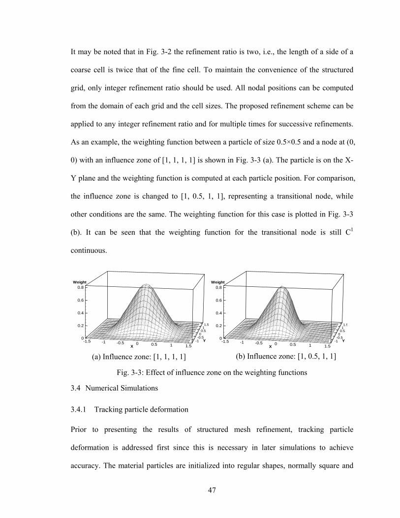
47
It may be noted that in Fig. 3-2 the refinement ratio is two, i.e., the length of a side of a
coarse cell is twice that of the fine cell. To maintain the convenience of the structured
grid, only integer refinement ratio should be used. All nodal positions can be computed
from the domain of each grid and the cell sizes. The proposed refinement scheme can be
applied to any integer refinement ratio and for multiple times for successive refinements.
As an example, the weighting function between a particle of size 0.5×0.5 and a node at (0,
0) with an influence zone of [1, 1, 1, 1] is shown in Fig. 3-3 (a). The particle is on the X-
Y plane and the weighting function is computed at each particle position. For comparison,
the influence zone is changed to [1, 0.5, 1, 1], representing a transitional node, while
other conditions are the same. The weighting function for this case is plotted in Fig. 3-3
(b). It can be seen that the weighting function for the transitional node is still C1
continuous.
Fig. 3-3: Effect of influence zone on the weighting functions
3.4 Numerical Simulations
3.4.1 Tracking particle deformation
Prior to presenting the results of structured mesh refinement, tracking particle
deformation is addressed first since this is necessary in later simulations to achieve
accuracy. The material particles are initialized into regular shapes, normally square and
(a) Influence zone: [1, 1, 1, 1] (b) Influence zone: [1, 0.5, 1, 1]
-1.5 -1 -0.5 0 0.5 1 1.5-1-0.500.511.5
0
0.2
0.4
0.6
0.8
Y
Weight
X-1.5 -1 -0.5 0 0.5 1 1.5
-1-0.500.511.5
0
0.2
0.4
0.6
0.8
Y
Weight
X
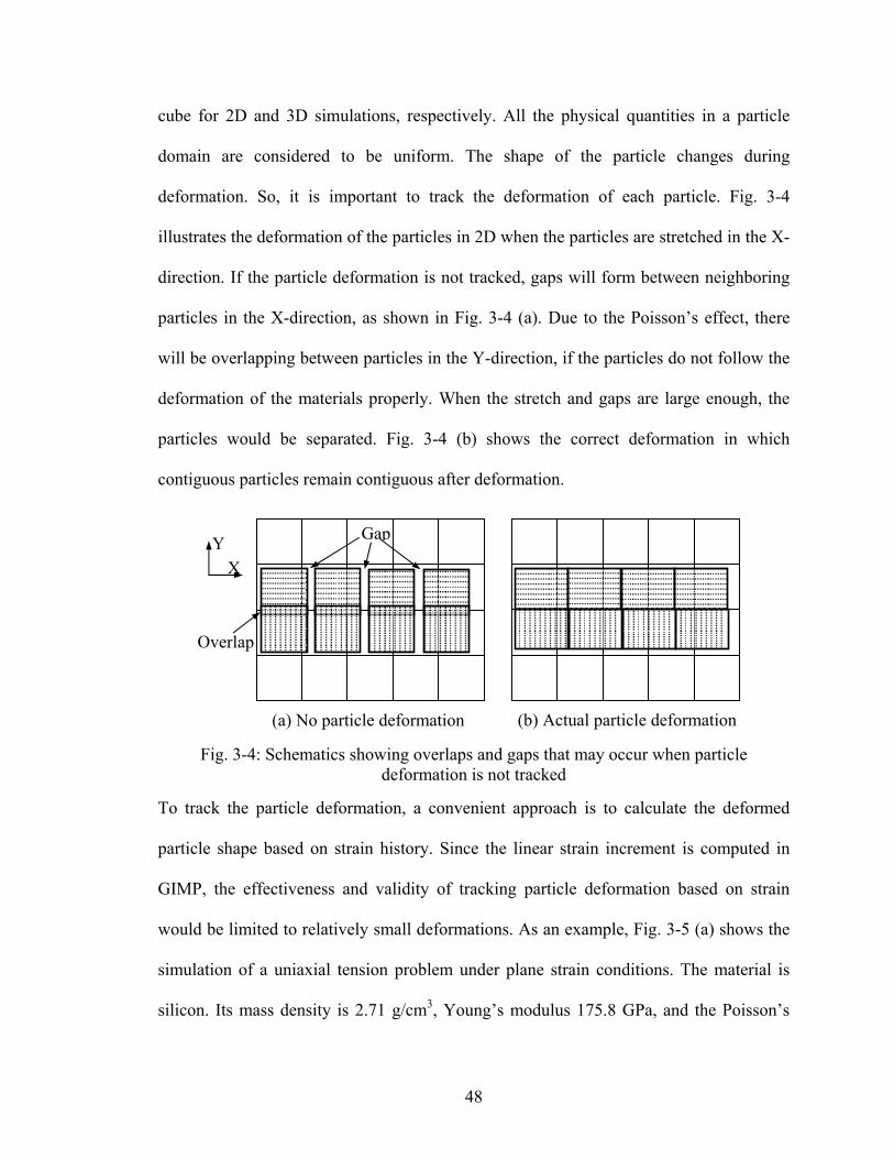
48
cube for 2D and 3D simulations, respectively. All the physical quantities in a particle
domain are considered to be uniform. The shape of the particle changes during
deformation. So, it is important to track the deformation of each particle. Fig. 3-4
illustrates the deformation of the particles in 2D when the particles are stretched in the X-
direction. If the particle deformation is not tracked, gaps will form between neighboring
particles in the X-direction, as shown in Fig. 3-4 (a). Due to the Poisson’s effect, there
will be overlapping between particles in the Y-direction, if the particles do not follow the
deformation of the materials properly. When the stretch and gaps are large enough, the
particles would be separated. Fig. 3-4 (b) shows the correct deformation in which
contiguous particles remain contiguous after deformation.
Fig. 3-4: Schematics showing overlaps and gaps that may occur when particle deformation is not tracked
To track the particle deformation, a convenient approach is to calculate the deformed
particle shape based on strain history. Since the linear strain increment is computed in
GIMP, the effectiveness and validity of tracking particle deformation based on strain
would be limited to relatively small deformations. As an example, Fig. 3-5 (a) shows the
simulation of a uniaxial tension problem under plane strain conditions. The material is
silicon. Its mass density is 2.71 g/cm3, Young’s modulus 175.8 GPa, and the Poisson’s
Overlap
X Y
(a) No particle deformation (b) Actual particle deformation
Gap

49
ratio 0.28. The background grid size is 0.002 × 0.002 mm2. One particle per cell is
assigned initially and the time step is 0.02 ns (1 ns = 10-9 s). The applied pressure
increases linearly with time from 0 to 10 ns and is then maintained constant, as shown in
Fig. 3-5 (b). The elongation in the X-direction of the particle is computed as 0)1( xx lε+ ,
where 0xl is the initial length of the particles. Separation of the particles occurred at ~25%
strain at 6 ns before the full pressure was applied, as shown in Fig. 3-5 (c). Similar
problems have been reported by Guilkey (2005).
Fig. 3-5: Simulation showing separation when the particle deformation is tracked by strain
Tracking particle deformation by strain could be more effective if nonlinear strain is used
in the GIMP method. However, recovery of the deformed shape based on nonlinear strain
involves additional complications. Based on the GIMP algorithm, there is another
convenient approach to track the particle deformation. Numerically, the displacement and
velocity of each particle in GIMP are computed at the center of the particle to represent
X
Y
L=0.06 mm
H=0.04
(a)
(c)
p
(b) t
p
40 GPa
0 10 ns
X
Y
0 0.02 0.04 0.06 0.08 0.10.01
0.02
0.03
0.04
0.05σx
95000855007600066500570004750038000285001900095000
Separation (MPa)
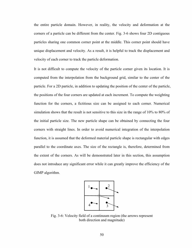
50
the entire particle domain. However, in reality, the velocity and deformation at the
corners of a particle can be different from the center. Fig. 3-6 shows four 2D contiguous
particles sharing one common corner point at the middle. This corner point should have
unique displacement and velocity. As a result, it is helpful to track the displacement and
velocity of each corner to track the particle deformation.
It is not difficult to compute the velocity of the particle corner given its location. It is
computed from the interpolation from the background grid, similar to the center of the
particle. For a 2D particle, in addition to updating the position of the center of the particle,
the positions of the four corners are updated at each increment. To compute the weighting
function for the corners, a fictitious size can be assigned to each corner. Numerical
simulation shows that the result is not sensitive to this size in the range of 10% to 80% of
the initial particle size. The new particle shape can be obtained by connecting the four
corners with straight lines. In order to avoid numerical integration of the interpolation
function, it is assumed that the deformed material particle shape is rectangular with edges
parallel to the coordinate axes. The size of the rectangle is, therefore, determined from
the extent of the corners. As will be demonstrated later in this section, this assumption
does not introduce any significant error while it can greatly improve the efficiency of the
GIMP algorithm.
Fig. 3-6: Velocity field of a continuum region (the arrows represent both direction and magnitude)
1 2
3 4

51
Fig. 3-7: GIMP results with tracking deformation of corners and their comparison with FEM
Using this approach to track the particle deformation, the problem in Fig. 3-5 (a) was
simulated again with GIMP and the results at 20 ns are plotted in Fig. 3-7 (a). No
separation of particles was seen during the entire simulation up to 50% strain. It is noted
that each material particle is plotted as a square of the same size and the particle
deformation is not shown due to software limitations on visualization. For comparison,
the same problem is simulated using FEM (Abaqus/Explicit) and the FE result is shown
in Fig. 3-7 (b). It can be seen that these two sets of results agree reasonably well with
each other; the maximum difference in maximum tensile stress is ~8%.
3.4.2 Indentation problem
To verify the refinement algorithm, a 2D indentation problem was simulated. Pressure is
applied at the top of the workpiece, as shown in Fig. 3-8. The dashed lines indicate the
(b) FEM
(MPa)
(a) GIMP

52
borders of refinement levels. The work material is silicon with the properties the same as
those given in the previous section. Due to symmetry with respect to the Y-axis, only half
of the workpiece is modeled. The size of the model is 0.027 × 0.04 mm2. The pressure
increases linearly with time from t = 0 - 30 ns and is then kept constant at 60 GPa.
Fig. 3-8: Two-dimensional indentation simulation
Several simulations were performed under different settings for the purpose of
comparison. In the first simulation, a uniform grid with a cell size of 0.001 × 0.001 mm2
is used and the time step is 20 ps (1 ps = 10–12 s). The stress distribution in the workpiece
at t = 20 ns is shown in Fig. 3-9 (a). In this figure, the units of length and stress are mm
and MPa, respectively. In the second simulation, as indicated in Fig. 3-9 (b), two levels of
refinements are used with the refinement ratio to be 2. The cell lengths are 0.002 mm and
0.001 mm for the first and second levels, respectively. The fine level covers a rectangular
area of the workpiece from (0, 0.02) to (0.02, 0.04). The grid is fixed in space; the
material particles initially in the fine region move to the coarse region during deformation.
As shown in Fig. 3-9 (b), some fine material particles have moved below the line Y =
0.02 mm. It may be noted that in Fig. 3-9 the material particles are plotted as squares
corresponding to their initial sizes. Gaps between particles are intentionally shown to
depict the particle sizes.
X
Y p
Level 2
Level 3
Sym
met
ry
p
t
60 GPa
0 30 ns
Level 1
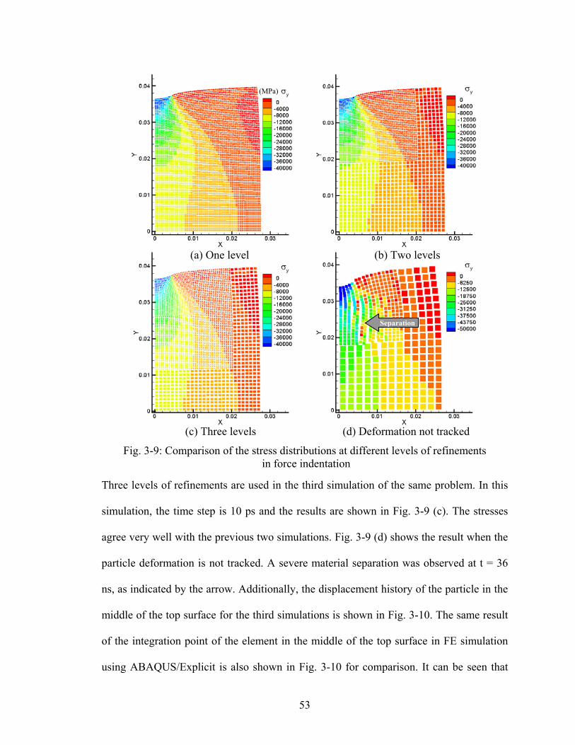
53
Fig. 3-9: Comparison of the stress distributions at different levels of refinements in force indentation
Three levels of refinements are used in the third simulation of the same problem. In this
simulation, the time step is 10 ps and the results are shown in Fig. 3-9 (c). The stresses
agree very well with the previous two simulations. Fig. 3-9 (d) shows the result when the
particle deformation is not tracked. A severe material separation was observed at t = 36
ns, as indicated by the arrow. Additionally, the displacement history of the particle in the
middle of the top surface for the third simulations is shown in Fig. 3-10. The same result
of the integration point of the element in the middle of the top surface in FE simulation
using ABAQUS/Explicit is also shown in Fig. 3-10 for comparison. It can be seen that
Separation
(b) Two levels (a) One level
(d) Deformation not tracked (c) Three levels
(MPa)

54
the displacement compares well with FE up to t = ~20 ns. After this time, FE simulation
aborted due to mesh distortion. This demonstrates the capability of GIMP using a grid
with structured refinement in handling large deformations.
Time (ns)
Uy(μ
m)
0 10 20 30 40-8
-6
-4
-2
0
GIMPFEM
FEM aborted
Fig. 3-10: Comparison of displacement history with FE
It may be noted that if the exterior corners of the surface particles are tracked from the
nodal interpolations in the same way as the interior corners, simulations tend to become
unstable due to erroneous surface corner displacements. This problem was observed to be
strictly and consistently associated with the particles with external tractions applied. It is
caused by insufficient nodal interpolation. To eliminate this problem, the exterior corners
of the surface particles were tracked by strain only, as used in these simulations.
3.4.3 Verification of the displacement boundary condition
Next, the results on the validation of the displacement boundary conditions are presented.
For dynamic simulations, an artificial damping may be introduced. With damping, the
nodal momentum can be updated as
td iuii
biii Δ−+++=Δ )( int pffffp τ , (3-16)
where d is the artificial damping coefficient.

55
A rectangular slab is fixed on the left and a displacement boundary condition is applied
on the right, as shown in Fig. 3-11. The material is silicon and its properties are given in
the previous section. The cell size in this simulation is 0.5 × 0.5 mm2 and four particles
are assigned to each cell initially. The time step is 5 ns. The prescribed displacement
increases linearly with time to 0.5 mm at t = 10 μs, which corresponds to a velocity of 50
m/s, and remains constant thereafter. This problem is simulated in FE using
Abaqus/Explicit for comparison. The displacement in the X-direction, Ux, for a particle
initially centered at (2.625, 1.625) as a function of time is plotted in Fig. 3-12 (a). It can
be seen that without damping, the vibrations of displacement from both FEM and GIMP
simulations are in phase before t = 14 μs, but out of phase afterwards. The dashed line
represents the steady state displacement at this point. It can be seen that when an artificial
damping of 106 s-1 is used, the GIMP solution converges quickly. The error of the
converged displacement is 0.46%. Fig. 3-12 (b) shows the comparison of the normal
stress in the X-direction. Good comparison between GIMP and FE has been obtained.
With damping, the GIMP solution converges to the analytical solution for static
simulations.
Fig. 3-11: A simple tension problem with displacement boundary conditions
X
Y L=6 mm
H=3 mm
u

56
Fig. 3-12: Comparisons of the displacement and stress
3.4.4 Stress concentration problem
Fig. 3-13 shows a copper plate (60 × 60 mm2) with a central hole (4 mm diameter)
subjected to a distributed load. This problem is simulated using GIMP as a dynamic
problem with a damping factor of 1000 s-1 and three levels of refinement. The cell sizes
at these three levels are 1.0 mm, 0.5 mm, and 0.25 mm, respectively. One particle is
assigned to each cell not adjacent to the hole initially. The cells close to the circular hole
are assigned 25 particles each to model the circular edge more accurately with the use of
square particles. It may be noted that all the particles occupy square areas initially. The
time step is 10 ns and the applied distributed load intensity p = 10 MPa.
Fig. 3-13: A plate with a circular hole subjected to tension
The stress distribution after 4000 steps is shown in Fig. 3-14 (a) and the area close to the
hole (bottom left corner in Fig. 3-14 (a)) is magnified in Fig. 3-14 (b). The normal stress
p p X
Y θ
Time (μs)
Ux(m
m)
0 10 20 30 400
0.05
0.1
0.15
0.2
0.25
0.3
GIMP d=0FE d=0GIMP d=106 1/sSteady State
(a) Displacement history Time (μs)
σ x
0 10 20 30 400
5
10
15
20
GIMP d=0FE d=0GIMP d=106 1/sSteady State
(GP
a)
(b) Stress history

57
of the particle at the top of the hole is 30.7 MPa when the applied tension is 10 MPa. This
gives a stress concentration factor of 3.07. The tangential stress of the particles along the
hole circumference, normalized by the applied pressure, is plotted in Fig. 3-15 in
comparison with the theoretical value (Pilkey (1997)). A good agreement between the
numerical simulation and theoretical value is obtained. This demonstrates that the GIMP
refinement algorithm is effective for problems involving significant stress gradients.
Furthermore, with the use of small square particles, GIMP is capable of modeling curved
surfaces
.
Fig. 3-14: Normal stress in the X-direction with p = 10 MPa
Angle θ (degrees)
Nor
mal
ized
Tang
entia
lStre
ss
0 15 30 45 60 75 90-2
-1
0
1
2
3
4NumericalTheoretical(Pilkey, 1997)
Fig. 3-15: Normalized tangential stress along the circumference of the hole
(a) Overall (b) Magnified
(MPa)

58
3.4.5 Static stress intensity factor
Next, the GIMP refinement algorithm is implemented to determine the stress field and
stress intensity factor for a mode I crack problem to determine the capability of the GIMP
refinement algorithm in simulation of stress distribution near a crack. Guo and Nairn
(2003) have successfully extended the MPM method to compute stress distribution in a
plate with explicit cracks using multiple nodal fields along the crack surface. The
physical quantities of material particles on each side of the crack were interpolated using
variables in the field on that side of crack surface. In their simulation, a uniform mesh
was used. Since the stress gradient at the crack tip is very high, a refined mesh near the
crack tip and a coarse mesh in the far field should lead to savings in computational time
while maintaining the same accuracy with the use of a uniform fine mesh. The fracture
problem is thus an appropriate problem to evaluate the refined GIMP algorithm. For this
purpose, the same fracture problem by Guo and Nairn (2003) using MPM is modeled,
that is, a double cantilever beam (DCB) with a crack as shown in Fig. 3-16.
Fig. 3-16: Geometry of a double cantilever beam with a crack
In the area close to the crack tip, finer meshes are used, while in the area far away from
the crack tip, coarse meshes are used. The thickness of the plate is 1 mm, thereby
justifying a plane stress condition for this problem. The material of the DCB is
L=10
2H=2a=5
X
YF
F
Unit: mm
Crack

59
considered to be homogeneous, isotropic, and linearly elastic. Its density, Young’s
modulus, and Poisson’s ratio are 1500 kg/m3, 2300 GPa, and 0.33, respectively. The
applied force is 4104 −×=F N and this results in a mode I crack problem. The static stress
intensity factor for the DCB can be calculated using the following equation (Kanninen
1973)
2/3
)2/3(32
HHaF
K I+
= . (3-17)
This problem has been simulated using MPM with uniform grids of three sizes, 4 mm, 2
mm, and 1 mm (Guo and Nairn (2003)). They have computed the energy release rate and
determined the stress intensity factor from J-integral. Their results indicate that the stress
intensity factor determined from finer grid is more accurate and closer to the theoretical
value.
In the mesh refinement GIMP algorithm used in this study, the energy release rate was
computed using the virtual crack closure technique (Rybicki and Kanninen (1977); Wang,
Karuppiah, Lu, Roy, and Komanduri (2005)). The energy released during an infinitesimal
crack growth of aΔ is assumed to be the energy required to close the crack to its initial
size. Hence, the energy release rate G is determined by
∫Δ
→ΔΔ⋅
Δ=
a
ada
aG
00)(
21lim uσn , (3-18)
where n is the crack surface normal. For the 2D mode I crack in the X-direction,
∫Δ
→ΔΔ⋅
Δ=
a
yyyaI dauσa
G00 2
1lim . (3-19)
In GIMP, the energy release rate can be computed as
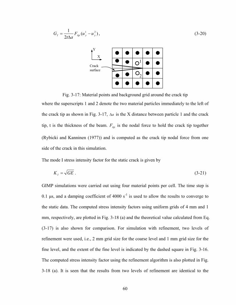
60
)(2
1 21yytipI uuF
atG −
Δ= , (3-20)
Fig. 3-17: Material points and background grid around the crack tip
where the superscripts 1 and 2 denote the two material particles immediately to the left of
the crack tip as shown in Fig. 3-17, aΔ is the X distance between particle 1 and the crack
tip, t is the thickness of the beam. tipF is the nodal force to hold the crack tip together
(Rybicki and Kanninen (1977)) and is computed as the crack tip nodal force from one
side of the crack in this simulation.
The mode I stress intensity factor for the static crack is given by
GEK I = . (3-21)
GIMP simulations were carried out using four material points per cell. The time step is
0.1 μs, and a damping coefficient of 4000 s-1 is used to allow the results to converge to
the static data. The computed stress intensity factors using uniform grids of 4 mm and 1
mm, respectively, are plotted in Fig. 3-18 (a) and the theoretical value calculated from Eq.
(3-17) is also shown for comparison. For simulation with refinement, two levels of
refinement were used, i.e., 2 mm grid size for the coarse level and 1 mm grid size for the
fine level, and the extent of the fine level is indicated by the dashed square in Fig. 3-16.
The computed stress intensity factor using the refinement algorithm is also plotted in Fig.
3-18 (a). It is seen that the results from two levels of refinement are identical to the
Crack surface
X
Y
1
2

61
results from one uniform fine level with 1 mm cell size. Moreover, the simulation time
using the refinement algorithm is 38% shorter than that of one uniform fine level. The
computed stress intensity factor became even closer to the theoretical value when a third
level of refinement was added for the crack tip as shown in Fig. 3-18 (b). For the case of
using uniform grid of 2 mm, the computed stress intensity factor using GIMP and MPM
(Guo and Nairn (2003)) are plotted in Fig. 3-19. The MPM results were computed using a
damping factor of 1000 s-1, and therefore, more oscillations can be seen as expected.
Fig. 3-18: Computed stress intensity factor as a function of time
Fig. 3-19: Comparison of the stress intensity factor with MPM results
(a) Overall (b) Magnified

62
Fig. 3-20: Stress distribution in the beam using three levels of refinements at t = 2.5 ms
Fig. 3-20 shows the distribution of σy at t = 2.5 ms when the force applied on the beam
was changed to 4=F N, 10000 times of the previous value, with other parameters the
same. In this simulation, three levels of refinements with cell sizes of 1 mm, 0.5 mm and
0.25 mm, were used and the different density of material points in each level can be
clearly seen in the figure. The computed stress intensity factor, scaled by 10000 times,
still compares well with the theoretical value. It is noted that deformation near the crack
surfaces has caused material points crossing cell boundaries, a situation where MPM
would give numerical noise such as alternating stress signs. Despite the extent of the
deformation, and material points crossing cell boundaries, GIMP method with the use of
particle deformation tracking still gives correct results, further verifying the structured
refinement methods developed herein.
3.5 Conclusions
1. A spatial refinement scheme for a structured grid was developed by adding transitional
nodes and by changing the influence zone of the transition nodes in GIMP. The influence
zone is square for uniform grid nodes and rectangular for transitional nodes. This
influence zone affects the computation of the nodal shape function. The computation of
the weighting function remains the same as for the uniform grid. The refinement scheme
(MPa)
Crack

63
can be applied successively and the refined grid remains structured in each refinement
level, i.e., every node can be determined by the extent of the grid level and cell size. The
refinement scheme was implemented and several problems such as tension, indentation,
stress concentration, and stress distribution near a crack (mode I crack problem) were
modeled to demonstrate its effectiveness and accuracy. A good agreement has been
obtained between numerical and theoretical results, indicating the validity of the
structured mesh refinement for GIMP scheme.
2. The GIMP algorithm has also been extended to include the displacement boundary
condition, based on the approach used in the meshless local Petrov-Galerkin (MLPG)
method, Atluri and Zhu (2000). A penalty parameter is used to impose the displacement
boundary condition and a nodal force vector because the displacement boundary
condition is introduced to the nodal momentum governing equation. A uniaxial tension
problem with constant pulling velocity was simulated to verify the displacement
boundary condition.
3. A method to track the material particle deformation was developed and verified in one
example. When the particle deformation is not tracked, artificial separation was observed
when the particle strain increases to a certain level. In tensile simulations, when the
normal strain is ~25%, material particles tend to separate from the body. Our approach
tracks the displacement of each corner of the material particles. Since neighboring
particles share corners, no separation would occur during deformation using this
approach.

64
Chapter 4
Simulation of Deformation Mechanism and Failure of Bulk Metallic Glass
(BMG) Foam Using the GIMP Method
A new bulk metallic glass (BMG) foam, processed by thermo-plastic expansion, has
recently been discovered (Schroers et al. (2003); Brothers and Dunand (2004); Hanan et
al. (2005)). In this investigation, the microstructure and mechanical properties of BMG
foam were determined using microtomography combined with in-situ compression.
Numerical simulation of the mechanisms of deformation and failure of the BMG foam,
which has never been done before, is conducted in this investigation. The complex
cellular geometry of the foam was modeled using the generalized interpolation material
point (GIMP) method by creating material points based on grayscales at voxels
determined from microtomography. Nanoindentation tests were conducted to determine
the local elastic modulus of the foam matrix and the results are used as the input to the
GIMP simulation. Several cubic volume elements (from 0.5763 mm3 to 1.7283 mm3)
taken from the 3D tomographic image were used in the simulation. The size of the cube
is increased until further increase in volume does not lead to a change in mechanical
response; the cube with this size is determined as the representative volume element. The
simulated compressive stress-strain curve using GIMP was compared with the
experimental data and a good agreement on the initial slope (representative of the average
Young’s modulus of the foam) was obtained. The stress contour in the foam was
65
illustrated by analyzing different sections of the foam at different simulation times. The
densification and hardening of the ductile metallic foam under compression was
simulated to demonstrate the capabilities of GIMP and to study the failure mechanisms.
4.1 Introduction
Metallic glass foam has been used in various engineering applications due to such
combination of unique properties as low density, high specific strength, high energy
absorption, and superior thermal insulation. Foam materials are generally divided into
open-cell and closed-cell foams. In general, open-cell foams have higher porosity and
softer behavior than closed-cell foams. The uniaxial mechanical behavior of a foam is
characterized by three regimes, namely, initial elastic response, the stress plateau that
follows, and final stiffening due to densification (Gibson and Ashby (1997); Miller
(2000); Katti et al. (2006)). Theoretical modeling of the foam mechanics has been carried
out for both regular and irregular open-cell foams. The nonlinear stress-strain relation of
the foams at high strains was modeled by the buckling of elastic cell edges (Zhu et al.
(1997)) or by the implementation of nonlinear kinematics (Wang and Cuitino (2000)).
Most numerical simulations of foam materials reported in the literature were either at the
macroscopic scale or the mesomechanical (micromechanical) scale. At the macroscopic
scale, the foam material is considered as a homogeneous material with homogenized
properties determined from measurements such as uniaxial compressions (Gibson (1997)).
The work using this approach is rather limited, due primarily to the well-known problem
associated with simulating cells in contact. In this approach, large foam structures can be
simulated at relatively low computational cost and the deformations under different
loading conditions can be predicted reasonably well (Meguid et al. (2002); Meguid et al.

66
(2004)). However, such simulations require knowledge of loading conditions a priori and
the associated material model may not be readily available in some situations (Wicklein
et al. (2004)).
In the mesomechanical simulations, the microstructure of the foam is modeled explicitly.
X-ray tomography is used to determine the three-dimensional (3D) microstructure and
the 3D geometry is used in a numerical model for simulation. In this approach, the
discrete element/particle size is dictated by the resolution of the X-ray tomography.
Kadar et al. (2004) investigated the mechanical behavior of closed-cell Al porous foam
by indentation using the finite element method (FEM). Wicklein and Thoma (2005)
conducted a series of FEM simulations and determined the elastic and plastic response of
an open-cell aluminum foam. The mesomechanical approach provides microstructural
evolution during deformation; however, the computational cost can be very high.
For model generation using mesomechanical simulation approach, Wicklein et al. (2004)
described three possible approaches to discretize a foam structure into FEM meshes. In
the first approach, beam and plate elements are constructed based on the cell votices in
the tomographic images. In the second approach, voxels are transformed into cubic
elements in a predefined structured mesh. In the third approach, tetrahedral elements are
used to mesh the entire foam structure. The second approach was used successfully for
the simulation of aluminum foams (Wicklein et al. (2004); Wicklein and Thoma (2005))
under a few percent deformations. However, simulation of a fully densified foam is a
challenge in FEM because of large distortions of the microstructure involved and the
internal contact of cell walls upon closure of cells. Brown et al. (2000) used hexahedral
elements to model the struts of an open-cell foam under impact loading. It was pointed

67
out that the drawbacks of this approach involve the use of a large number of elements and
small time-steps. It is noted that the struts all have regular cross sections so that it was
relatively easy to mesh all the struts.
Recently, the generalized interpolation material point (GIMP) method was introduced for
dynamic simulation of materials (Bardenhagen and Kober (2004); Ma et al. (2005)).
GIMP has evolved from the material point method (MPM), originally developed by
Sulsky, Zhou and Schreyer (1995) and subsequently refined by others (e.g., Tan and
Nairn (2002); Wang et al. (2005)). In GIMP, the workpiece is discretized into a
collection of material particles (points). The material points carry all the physical
variables, including the mass, momentum and stress, in the simulation. A background
grid, usually a structured grid fixed in space, is used to discretize the momentum
conservation equation and solve it at the grid nodes using explicit time integration. In a
regular GIMP computational step, the material point information is first interpolated to
the grid nodes. Then, the momentum conservation equation is solved at the nodes to
update the nodal information. Next, the updated nodal information is interpolated to
update the position, velocity, strain, and stress at the material points. Finally, the
background grid is redefined (usually reset the nodal quantities to zero but keep the nodal
positions fixed). GIMP shares some similarities with other meshless methods, e.g., Atluri
and Zhu (2000). Fig. 4-1 (a) illustrates an elliptical workpiece discretized into a
collection of material points of different sizes with the background grid shown. When
two bodies are close enough, as indicated by open and closed circles in Fig. 4-1 (b), the
material point information will be interpolated to the same grid node in the middle when
one background is used. In this case, these two workpieces are in non-slip contact. The

68
intrinsic features associated with GIMP, such as ease of discretization, no body-fixed
meshes used so that mesh distortion is not an issue and natural capability of handling
non-slip contact, made the simulation of some complex problems possible.
Fig. 4-1: Illustrations of the discretization scheme and intrinsic contact in GIMP
GIMP was used successfully to simulate densification of open-celled foam materials
(Bardenhagen et al. (2005); Brydon et al. (2005)). In GIMP simulations, each voxel in
the X-ray tomograph is converted into a material particle and an Eulerian structured grid
is used for solving the field equations. A representative volume element (RVE) was used
to simulate the bulk response of a foam. Their results have indicated that the apparent
Poisson’s ratio is negative in the stress plateau and the dynamic response of the
compression is dominated by a compression wave, which is an inertial effect absent in
homogeneous material and its velocity is much slower than any characteristic wave
speeds (Brydon et al. (2005)).
In this work, we report the results of a simulation of a closed-cell foam made of bulk
metallic glass. Most metal and its alloys in engineering applications are in the form of
crystalline structures; their mechanical properties are dependent on the crystal structure,
chemistry, microstructure, and processing conditions. Metallic glass is another form of a
metal or an alloy. In a metallic glass, the material is amorphous and has no long-range
atomic order. Fig. 4-2 (a) and (b) are TEM images of the microstructure of a crystalline
(a) Discretization and background grid (b) Non-slip contact

69
zirconium alloy and the same alloy in the amorphous form (Hufnagel (2005)). Metallic
glass can be formed by rapid cooling of a liquid metal; the cooling rate is so high that
ordered crystalline structure cannot be developed in the metal, resulting in amorphous
structures.
Fig. 4-2: High resolution TEM images of (a) crystalline and (b) amorphous structures of a zirconium alloy (Hufnagel (2005))
Metallic glass foams recently have attracted great attention due to their unique properties.
They exhibit high specific strength, high stiffness, high energy absorption (Ashby et al.
(2000)), and more importantly they can be used under those conditions, including, high
temperatures where other foams (e.g., polymer foams) cannot be used. BMG foams
combine exceptional strength, elasticity, wear, and corrosion resistance with modest
densities and low processing temperatures. They are being considered for structural and
biocompatible implant applications (Hanan et al. (2005); Brother and Dunand (2005)).
The thickness of BMG material is usually limited (on the order of a few millimeters to a
centimeter or so) by the requirement that a high enough cooling rate in the center of the
wall is necessary to form the amorphous structures. For a pore-free BMG
(Pd42.5Cu30Ni7.5P20), Wada, Inoue and Greer (2005) reported a Young’s modulus of 102
(a) Crystalline (b) Amorphous

70
GPa, failure stress of 1.63 GPa, zero plastic strain and the rupture energy density of 14
MJ/m3. Their results show that with increase in porosity of the BMG rod, both Young’s
modulus and failure stress decrease while plastic strain at failure and rupture energy
increase.
Research on BMG foams has been focused primarily on improving mechanical behavior
and testing. BMG foam expansion tests are being carried out in outer-space and BMG
foams are found to be suitable for some space-vehicle related applications. Numerical
simulations of metallic glass foams are rather limited due to difficulties in modeling
complex internal structures and handling large deformations as well as contacts. In this
investigation, we utilize the unique features of GIMP to simulate the behavior of a BMG
foam, which has never been done before. The metallic glass foam considered in this
investigation is a closed-cell, amorphous BMG foam (Pd43Ni10Cu27P20) prepared by
thermo-plastic expansion using B2O3-XH2O as a blowing agent (Hanan et al. (2005)).
Compression of the metallic glass foam was simulated using the GIMP method with
parallel processing. The simulated results are compared with the experimental data to
verify the simulation technique.
4.2 Nanoindentation Testing of BMG Foam
The Young’s modulus of the BMG foam is an input used in the GIMP simulation. The
data is determined from direct measurement of the Young’s modulus of the cell-wall of
the BMG foam using nanoindentation. A BMG sample was wrapped in epoxy, then cut
and polished carefully to expose its walls. Nanoindentation was made using a Berkovich
indenter at an indentation depth of 510 nm. To satisfy the condition of indentation on a
half-space, indentations were made only on relatively thick walls. Fig. 4-3 shows the

71
average load-depth curve with error bars for all the five nanoindentations. Table 4-1 lists
the measured Young’s modulus and hardness for the BMG foam. The load-depth curve
shows good consistency when the depth is < 300 nm; but the deviation becomes larger at
higher depths. This can be due to the presence of a thin wall at one location which can
deflect excessively or buckle locally with increase in the indentation load. For this reason,
the modulus and hardness from each nanoindentation test were averaged over the depths
from 100 nm to 350 nm. It is found that modulus of the foam material does not depend on
the location in the BMG foam. To simplify the simulation, it is assumed that within the
walls the material properties are homogeneous and isotropic with a Young’s modulus of
108.1 GPa.
Displacement (nm)
Load
(mN
)
0 100 200 300 400 500 6000
5
10
15
20
25
30
Fig. 4-3: Average nanoindentation load-displacement curve with error bars for the BMG foam (Pd43Ni10Cu27P20)
Table 4-1: Nanoindentation results for the BMG foam.
Test 1 2 3 4 5 Mean Modulus (GPa) 107.36 98.96 108.23 108.09 117.86 108.1 Hardness (GPa) 8.49 5.29 7.22 8.42 8.13 7.5
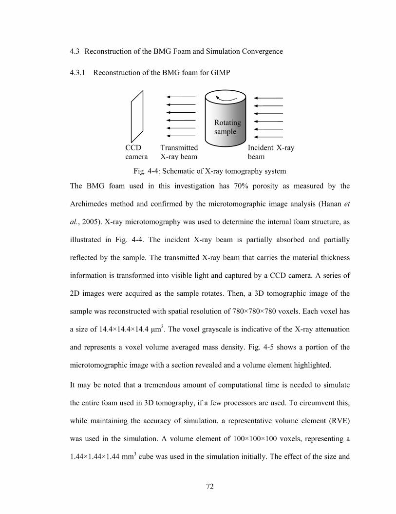
72
4.3 Reconstruction of the BMG Foam and Simulation Convergence
4.3.1 Reconstruction of the BMG foam for GIMP
Fig. 4-4: Schematic of X-ray tomography system
The BMG foam used in this investigation has 70% porosity as measured by the
Archimedes method and confirmed by the microtomographic image analysis (Hanan et
al., 2005). X-ray microtomography was used to determine the internal foam structure, as
illustrated in Fig. 4-4. The incident X-ray beam is partially absorbed and partially
reflected by the sample. The transmitted X-ray beam that carries the material thickness
information is transformed into visible light and captured by a CCD camera. A series of
2D images were acquired as the sample rotates. Then, a 3D tomographic image of the
sample was reconstructed with spatial resolution of 780×780×780 voxels. Each voxel has
a size of 14.4×14.4×14.4 μm3. The voxel grayscale is indicative of the X-ray attenuation
and represents a voxel volume averaged mass density. Fig. 4-5 shows a portion of the
microtomographic image with a section revealed and a volume element highlighted.
It may be noted that a tremendous amount of computational time is needed to simulate
the entire foam used in 3D tomography, if a few processors are used. To circumvent this,
while maintaining the accuracy of simulation, a representative volume element (RVE)
was used in the simulation. A volume element of 100×100×100 voxels, representing a
1.44×1.44×1.44 mm3 cube was used in the simulation initially. The effect of the size and
Rotating sample
Incident X-ray beam
Transmitted X-ray beam
CCD camera

73
location of the volume element were investigated subsequently. The solid Pd-based BMG
has a density of 9.44 g/cc. Material points are assigned to areas occupied by the BMG
foam matrix. The use of a cut-off grayscale value of 100 gave a porosity of 70% for the
BMG foam, same as the porosity determined by other methods. There are about 300,000
material points in the volume element for this GIMP model. Fir the simulations 12
processors (Pentium IV, 2.4 GHz; 512 MB memory) were used in the simulations and the
computational domain was divided into approximately equal-sized blocks, e.g., 3, 2, 2 in
the X-, Y-, and Z- directions, respectively. Details on the parallel processing in GIMP can
be found in Ma et al. (2005).
Fig. 4-5: 3D microtomographic image of a BMG foam
Each voxel occupied by the material is assigned a material point. The mass density and
Young’s modulus of each material point are dependent on the grayscale of the voxel. The
mass density of the material point is assumed to be linearly dependent on the grayscale.
The Young’s modulus of each material point is assumed to obey a power law relation
with the grayscale, i.e.,
~10 mm

74
EI
sEn
p ⎟⎟⎠
⎞⎜⎜⎝
⎛=
max
, (4-1)
where s is the grayscale of a voxel and 255 ( maxI ) is the maximum grayscale
corresponding to the density of the bulk solid material. When the exponent n = 1, the
modulus is linearly dependent on the grayscale. This is consistent with the rule of
mixtures (Jones (1999)) where each voxel is occupied by the material and air. For a
closed-cell foam, the modulus for a volume element containing a pore can be
proportional to the square of the volume fraction (Gibson and Ashby (1997); Wicklein
and Thoma (2005)). Hence, in this study, the exponent n = 2 is also simulated for
comparison. The Young’s modulus E used for the BMG foam is 108.1 GPa as determined
from nanoindentation.
4.3.2 Effect of grid cell size on simulation convergence
In GIMP simulation, the accuracy improves with finer background grid since momentum
conservation equation is solved at each grid node. In the GIMP computation,
interpolation of physical variables is made between material points and their neighboring
nodes. The computational time is dependent directly upon the number of background grid
nodes and the grid size. When the grid size is small, physical variables of material points,
such as the stresses and stains are interpolated on a large number of grid nodes resulting
in more computations. Numerical simulations were first conducted to determine the effect
of grid size on accuracy. A normal traction of 50 MPa was applied at one end of the
sample in the Z-direction to pull the sample. The time step was 0.5 ns and the numerical
damping factor used was 1000 s-1.

75
Fig. 4-6: Stress distribution on a section simulated with the grid size of 3 and 4 times of the voxel size, respectively
The normal stress zσ on a given cross section after 1000 increments is plotted in Fig. 4-6
using grid sizes of 3 and 4 times the voxel size (14.4 μm), respectively, in each direction.
In Fig. 4-6 (a) and (b), stress variations, as indicated by the dashed circles, can be seen.
These stress variations are unphysical due to incorrect interactions of the material points
near the pores. These results indicate that the grid size is too large. It may be noted that
the surface of a pore is traction free; but if the grid is too coarse, the material points on
both sides of a pore can interact with each other through the grid node, resulting in non-
zero traction on the surface of a pore and violating the traction-free conditions on the
surface. To circumvent this problem, smaller grid sizes were investigated. Fig. 4-7 (a)
and (b) show the normal stress distribution on the same section as used in Fig. 4-6, but
simulated with the grid size of 1 and 2 voxels, respectively, in each coordinate direction.
The results show that the transition is smooth. Comparing Fig. 4-7 (a) and (b), it can be
seen that zσ stress is almost zero on the pore top/bottom surfaces when the grid size is 1
voxel, which means that the traction free boundary condition on the surface of each pore
(a) Grid size is 3 voxels (b) Grid size is 4 voxels X
Z

76
is nearly satisfied.
Fig. 4-7: Stress distribution on a section simulated with the grid size to be 1 and 2 times of the voxel size.
The average computational times per time step were 8.8, 9.2, 10.5, and 13 s for grid sizes
of 4, 3, 2 and 1 voxel, respectively, all other conditions remaining the same. It is seen that
the computational time increases with decrease in grid size. Brydon et al. (2005) showed
that if the grid size is two thirds of the voxel size, then there is no appreciable
improvement in accuracy. For a balance between accuracy and computational time, the
grid size was chosen to be one voxel size in later simulations.
4.4 Simulation of the BMG Foam in Compression
In this section, we describe simulation of the BMG foam in compression. A velocity
boundary condition was applied at the top of the volume element using the penalty
method introduced by Ma et al. (2006). For the purpose of improving numerical stability,
12 uniform layers of extra materials were added at the top of the volume element and the
velocity boundary condition was applied on the top surface. The velocity in the quasi
static experiment was ~1 mm/s. A cylindrical sample was used with the load applied in
the Z-direction as shown in Fig. 4-8 (a). Fig. 4-8 (b) shows the nominal compressive
(a) Grid size is 1 voxel (b) Grid size is 2 voxels

77
stress-strain relationship of the BMG foam under uniaxial compression. There is no
plateau region in the curve and at a compressive strain of ~3.5%, a sudden drop in stress
is seen, corresponding to slip failure at the macroscopic level on a plane foaming a ~45
degree angle with the axis of the cylindrical sample. The unloading curve is nearly
parallel to the loading curve. The residual strain is ~2% when the sample is fully
unloaded, indicating the existence of a global plastic deformation in the foam. It may be
noted that the foam can be loaded continuously after the slippage. It will reach the plateau
region with multiple slippages, and eventually stiffen as the walls of the internal pores are
all compressed together.
Fig. 4-8: Experimental setup and nominal stress-strain curve.
The time step, dt used in the simulation was 0.5 ns, which was determined from the
longitudinal wave speed, lC and the grid size, gL , through lg CLkdt /⋅= , where k is a
constant factor (≤ 1) and the longitudinal wave speed of bulk BMG is 3926 m/s. If the
actual velocity used in the experiment was taken in the simulation, the computational
time would be very long to reach a compressive strain of 10% because a very large
number of time increments would be required due to the small time step used. To reduce
the computational time, the maximum velocity applied was set at 20 m/s, which is ~0.5%
x
z y
(a) (b)
Sample
Anvil
Compressive Strain
Com
pres
sive
Stre
ss(M
Pa)
0 0.01 0.02 0.03 0.04 0.050
20
40
60
80
100
120
Loading Slipping
Unloading

78
of the longitudinal wave speed of the bulk BMG. The applied velocity increased linearly
from 0 to 20 m/s in 10 μs to reduce the initial impact. From the simulation, the total force
F was computed as
∑=i
iiA nσF , (4-2)
where Ai is the area of the top surface of each material point i, n = (0,0,1) is the unit
outward normal vector, and the summation is performed over all the material points on
the top surface. The summation is performed over all the material points on the actual top
cellular layer of the volume element. The average stress is the total force F divided by the
gross cross sectional area. The average compressive strain was computed as the average
relative displacement of both cellular end surfaces divided by the initial height of the
cellular volume element.
4.4.1 Material failure
The bulk metallic glass (BMG) alloy is highly elastic and the plastic strain at failure is
nearly zero in compression (Wada and Inoue (2005)). The ductility of BMG can be
improved by introducing micro pores. Wada and Inoue (2005) reported that the plastic
strain at failure increases to more than 18% with increase in porosity from 0% to 3.7%.
The porosity of BMG foams can reach as high as 80%. The ductility of the BMG foams
under uniaxial compression is significantly higher than under tension. Wada and Inoue
(2003) reported 90% nominal compressive strain without macroscopic failure and
Brothers and Dunand (2005) reported 50% nominal compressive strain for several BMG
foams.
The ductility and failure strain of the BMG used in this study have been reported to

79
depend on the wall thickness (Conner et al., (2003)). In the simulation, the yield strength
of the material is assumed to be 1.63 GPa. Isotropic bilinear hardening is used and the
hardening modulus is assumed to be 5% of the Young’s modulus based on the
measurements on similar materials (Wada and Inoue (2005)).
4.4.2 Stress flow in the foam
Two locations in the foam were chosen in the simulations. The first location encompasses
the slip plane as observed in in-situ tomography of the foam in compression, and the
second location is far away from the slip plane. In this simulation, material failure is not
introduced, i.e., the foam is assumed purely elastic. Fig. 4-9 shows the stress distribution
in the overall 3D GIMP model at t = 2.5 μs in location 1.
Fig. 4-9: Stress distribution in the overall GIMP model at t = 2.5 μs at location 1.
The stress and deformation distributions in the BMG foam were determined for each
cross section. For the purpose of simplicity in discussion, each section is identified by its
normal direction and a number. The number between 0 and 100 indicates the percentage
location of the section along the specified direction. For example, section X-20 represents

80
the cross section perpendicular to the X-axis and located at 20% of the depth of the
sample size in the X-direction. Fig. 4-10 shows the zσ stress distribution of two sections
at t = 2.5 μs when the average compressive strain is 0.625%. zσ stress tends to align
with the available vertical paths. About 50% of the foam carries load, while the rest does
not play much role in carrying the load at this time. Along the path where the stress is
higher, the foam wall is generally thinner.
Fig. 4-10: Stress distribution on different sections at t = 2.5 μs.
Fig. 4-11: Stress distribution on different sections at 8% strain.
At t = 12 μs, the average compressive strain was 8%. The normal stress zσ distributions
(a) Section X-20 (b) Section X-40
(a) Section X-20 (b) Section X-40

81
at two sections are shown in Fig. 4-11. The maximum compressive stress in the volume
element was over 10 GPa which is much larger than the failure stress of 1.6 GPa as
reported by Wada et al. (2005). This is primarily due to the fact that material failure was
not introduced in the simulation. It was observed in this simulation that high stresses
appeared only at a few isolated spots in the sections.
4.4.3 The minimum size of a representative volume element (RVE)
Several simulations were conduced using volume element of different sizes in an effort to
determine the minimum size of a representative volume element (RVE). At two locations,
five different RVE sizes, namely, 40, 60, 80, 100 and 120 voxels in each coordinate
direction were used in simulations. The computed porosity for each size at both locations
is shown in Table 4-2. It may be noted that porosity for different sizes at each location
deviates from the nominal value due to random internal structure of the BMG foam; but
as the size increases to 120 voxels, the porosity at these two locations converge to values
very close to 70%, the nominal porosity of the foam. It may be noted that pore size and
shape vary significantly. The maximum dimension of the pores was found to be ~1.15
mm, equivalent to 80 voxel lengths. The aspect ratio, defined by the maximum dimension
divided by the minimum dimension, can be as large as 6 to 10. The medium pore
dimension was observed to be ~0.23 mm, equivalent to 16 voxel lengths.
Table 4-2: Porosity of different volume elements at each location.
Size 40 60 80 100 120 Location 1 78.7% 73.0% 73.2% 73.4% 71.4% Location 2 72.8% 69.8% 69.3% 70.2% 70.4%

82
Fig. 4-12: Stress-strain curves of the BMG foam from experiments and simulations using second order interpolation
Fig. 4-12 shows the stress-strain curves from simulations using second order interpolation
of the modulus, i.e., n = 2 in Eq. (4-1). It is seen that the slopes from simulations are all
smaller than the slope of the initial loading portion of the experimental curve. It is seen
that the simulation curves from volume elements of sizes 60, 80, and 100 are almost the
same at location 2. The slope obtained from a volume element of 40 voxels is much
smaller at this location. From Table 4-2, the RVE porosity at location 2 does not vary
much when the RVE size is between 60 and 120. The macroscopic yield strength
Compressive Strain
Com
pres
sive
Stre
ss(M
Pa)
0 0.01 0.02 0.03 0.04 0.050
20
40
60
80
100
120
140ExperimentP2-Size40P2-Size60P2-Size80P2-Size100
(b) Location 2
Compressive Strain
Com
pres
sive
Stre
ss(M
Pa)
0 0.01 0.02 0.03 0.04 0.050
20
40
60
80
100
120
140ExperimentP1-Size40P1-Size60P1-Size80P1-Size100P1-Size120
(a) Location 1

83
determined from a volume element of 100 voxels is close to the stress at the onset of
macroscopic collapse in experiment. At location 1, where the slip plane was observed, the
slopes increase with the sizes of the volume element. The 120-voxel element, at location
1, gives the converged stress-strain curve, comparable to that at location 2.
Fig. 4-13: Stress-strain curves of the BMG foam from experiments, model prediction and simulations using linear interpolation
Fig. 4-13 shows the simulation results using linear interpolation for the modulus of each
material point. It is seen that the stress is higher at the same strain when the volume
element is bigger at location 1. For the size of 120, the compressive stress-strain curve is
Compressive Strain
Com
pres
sive
Stre
ss(M
Pa)
0 0.01 0.02 0.03 0.04 0.050
20
40
60
80
100
120
140ExperimentP2-Size60P2-Size80P2-Size100P2-Size120
(b) Location 2
Compressive Strain
Com
pres
sive
Stre
ss(M
Pa)
0 0.01 0.02 0.03 0.04 0.050
20
40
60
80
100
120
140ExperimentP1-Size60P1-Size80P1-Size100P1-Size120
(a) Location 1
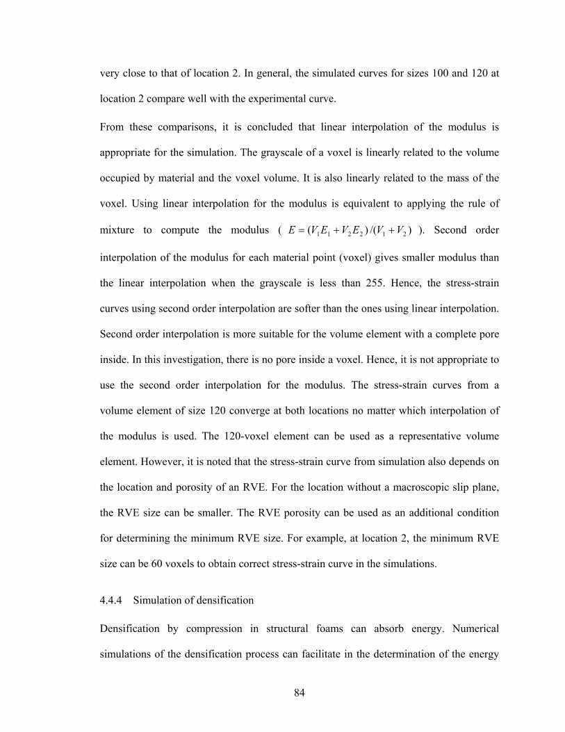
84
very close to that of location 2. In general, the simulated curves for sizes 100 and 120 at
location 2 compare well with the experimental curve.
From these comparisons, it is concluded that linear interpolation of the modulus is
appropriate for the simulation. The grayscale of a voxel is linearly related to the volume
occupied by material and the voxel volume. It is also linearly related to the mass of the
voxel. Using linear interpolation for the modulus is equivalent to applying the rule of
mixture to compute the modulus ( )/()( 212211 VVEVEVE ++= ). Second order
interpolation of the modulus for each material point (voxel) gives smaller modulus than
the linear interpolation when the grayscale is less than 255. Hence, the stress-strain
curves using second order interpolation are softer than the ones using linear interpolation.
Second order interpolation is more suitable for the volume element with a complete pore
inside. In this investigation, there is no pore inside a voxel. Hence, it is not appropriate to
use the second order interpolation for the modulus. The stress-strain curves from a
volume element of size 120 converge at both locations no matter which interpolation of
the modulus is used. The 120-voxel element can be used as a representative volume
element. However, it is noted that the stress-strain curve from simulation also depends on
the location and porosity of an RVE. For the location without a macroscopic slip plane,
the RVE size can be smaller. The RVE porosity can be used as an additional condition
for determining the minimum RVE size. For example, at location 2, the minimum RVE
size can be 60 voxels to obtain correct stress-strain curve in the simulations.
4.4.4 Simulation of densification
Densification by compression in structural foams can absorb energy. Numerical
simulations of the densification process can facilitate in the determination of the energy
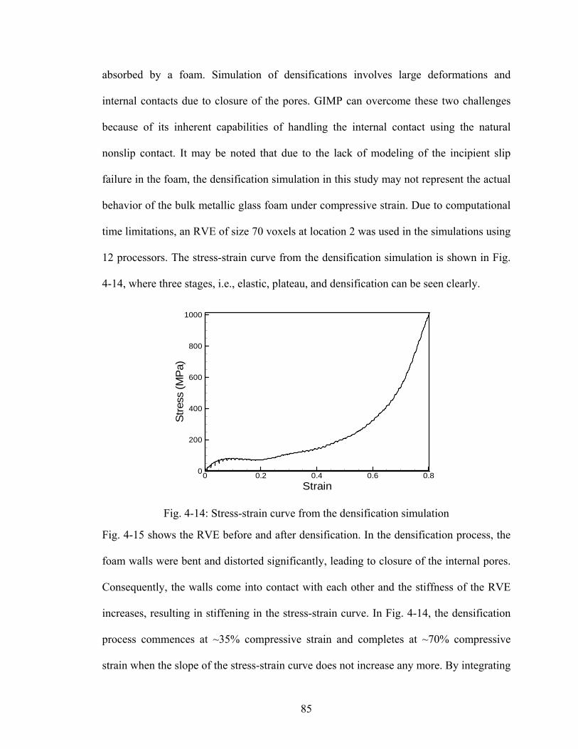
85
absorbed by a foam. Simulation of densifications involves large deformations and
internal contacts due to closure of the pores. GIMP can overcome these two challenges
because of its inherent capabilities of handling the internal contact using the natural
nonslip contact. It may be noted that due to the lack of modeling of the incipient slip
failure in the foam, the densification simulation in this study may not represent the actual
behavior of the bulk metallic glass foam under compressive strain. Due to computational
time limitations, an RVE of size 70 voxels at location 2 was used in the simulations using
12 processors. The stress-strain curve from the densification simulation is shown in Fig.
4-14, where three stages, i.e., elastic, plateau, and densification can be seen clearly.
Strain
Stre
ss(M
Pa)
0 0.2 0.4 0.6 0.80
200
400
600
800
1000
Fig. 4-14: Stress-strain curve from the densification simulation
Fig. 4-15 shows the RVE before and after densification. In the densification process, the
foam walls were bent and distorted significantly, leading to closure of the internal pores.
Consequently, the walls come into contact with each other and the stiffness of the RVE
increases, resulting in stiffening in the stress-strain curve. In Fig. 4-14, the densification
process commences at ~35% compressive strain and completes at ~70% compressive
strain when the slope of the stress-strain curve does not increase any more. By integrating
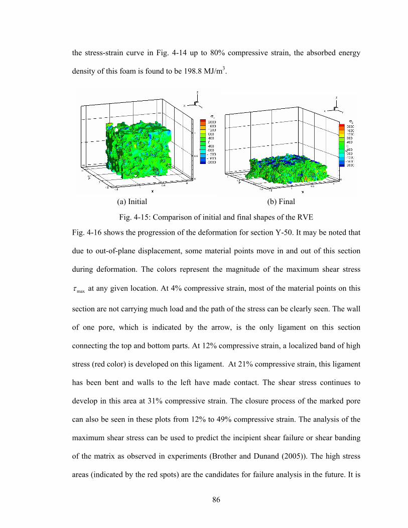
86
the stress-strain curve in Fig. 4-14 up to 80% compressive strain, the absorbed energy
density of this foam is found to be 198.8 MJ/m3.
Fig. 4-15: Comparison of initial and final shapes of the RVE
Fig. 4-16 shows the progression of the deformation for section Y-50. It may be noted that
due to out-of-plane displacement, some material points move in and out of this section
during deformation. The colors represent the magnitude of the maximum shear stress
maxτ at any given location. At 4% compressive strain, most of the material points on this
section are not carrying much load and the path of the stress can be clearly seen. The wall
of one pore, which is indicated by the arrow, is the only ligament on this section
connecting the top and bottom parts. At 12% compressive strain, a localized band of high
stress (red color) is developed on this ligament. At 21% compressive strain, this ligament
has been bent and walls to the left have made contact. The shear stress continues to
develop in this area at 31% compressive strain. The closure process of the marked pore
can also be seen in these plots from 12% to 49% compressive strain. The analysis of the
maximum shear stress can be used to predict the incipient shear failure or shear banding
of the matrix as observed in experiments (Brother and Dunand (2005)). The high stress
areas (indicated by the red spots) are the candidates for failure analysis in the future. It is
(a) Initial (b) Final
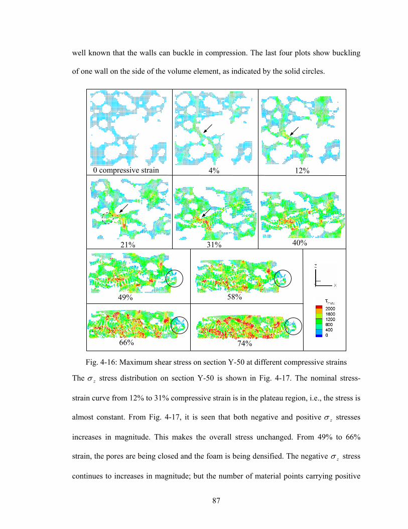
87
well known that the walls can buckle in compression. The last four plots show buckling
of one wall on the side of the volume element, as indicated by the solid circles.
Fig. 4-16: Maximum shear stress on section Y-50 at different compressive strains
The zσ stress distribution on section Y-50 is shown in Fig. 4-17. The nominal stress-
strain curve from 12% to 31% compressive strain is in the plateau region, i.e., the stress is
almost constant. From Fig. 4-17, it is seen that both negative and positive zσ stresses
increases in magnitude. This makes the overall stress unchanged. From 49% to 66%
strain, the pores are being closed and the foam is being densified. The negative zσ stress
continues to increases in magnitude; but the number of material points carrying positive
0 compressive strain 4%
21% 40%
49% 58%
66% 74%
12%
31%
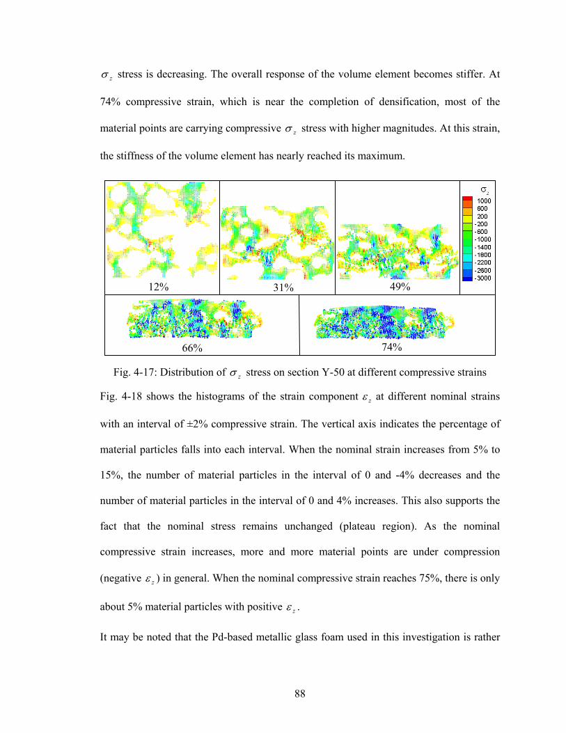
88
zσ stress is decreasing. The overall response of the volume element becomes stiffer. At
74% compressive strain, which is near the completion of densification, most of the
material points are carrying compressive zσ stress with higher magnitudes. At this strain,
the stiffness of the volume element has nearly reached its maximum.
Fig. 4-17: Distribution of zσ stress on section Y-50 at different compressive strains
Fig. 4-18 shows the histograms of the strain component zε at different nominal strains
with an interval of ±2% compressive strain. The vertical axis indicates the percentage of
material particles falls into each interval. When the nominal strain increases from 5% to
15%, the number of material particles in the interval of 0 and -4% decreases and the
number of material particles in the interval of 0 and 4% increases. This also supports the
fact that the nominal stress remains unchanged (plateau region). As the nominal
compressive strain increases, more and more material points are under compression
(negative zε ) in general. When the nominal compressive strain reaches 75%, there is only
about 5% material particles with positive zε .
It may be noted that the Pd-based metallic glass foam used in this investigation is rather
12% 49%
66% 74%
31%

89
brittle than the ductile Zr-based foams. The stress-strain curve in Fig. 4-14 represents the
response for more ductile metallic foams such Zr-based foams (Brother and Dunand
(2006)).
Fig. 4-18: Histograms of zε at three compressive strains
4.5 Conclusions
εz
-0.8 -0.6 -0.4 -0.2 0 0.20
20
40
60
80
100
εz
-0.8 -0.6 -0.4 -0.2 0 0.20
20
40
60
80
100
εz
-0.8 -0.6 -0.4 -0.2 0 0.20
20
40
60
80
100
5% nominal strain
εz
-0.8 -0.6 -0.4 -0.2 0 0.20
20
40
60
80
100
εz
-0.8 -0.6 -0.4 -0.2 0 0.20
20
40
60
80
100
εz
-0.8 -0.6 -0.4 -0.2 0 0.20
20
40
60
80
100
15%
75% 60%
45% 30%

90
The GIMP method is used to simulate the response of BMG foam (Pd43Ni10Cu27P20)
under compression. The complex internal structure of the foam is modeled using material
points generated from the 3-D tomographic images. Different background grid sizes were
evaluated and it was found that when the grid size is the same as the voxel size, high
simulation accuracy is achieved. A volume element of the full sample was taken for
compression simulation to compare with experiments. Numerical tests showed that linear
interpolation of the Young’s modulus for each material point is appropriate for the
simulation. The size of the volume element as well as the porosity of the corresponding
volume element can affect the simulated stress-strain curve of the foam. The minimum
size of the representative volume element (RVE) was determined by matching the
simulated stress-strain curve with the experimental data. Simulation of the full
compression of an RVE was conducted to investigate the densification process. Results
indicate that densification of the foam starts at ~35% compressive strain, which is
indicated by the gradual increase of stress and is completed at ~70% compressive strain.
The maximum shear stress on the pore walls is consistent with the experimental
observations of incipient shear band. The simulation approach presented in this paper can
be used to effectively simulate a variety of foam materials under different loading
conditions, such as tension, shear, and impact to predict the material behavior under
complex loading conditions.

91
Chapter 5
Multiscale Simulation Using GIMP Method and Molecular Dynamics
A new method for multiscale simulation bridging two scales, namely the continuum scale
using the generalized interpolation material point (GIMP) method and the atomistic scale
using the molecular dynamics (MD), is presented and validated in 2D. The atomistic
strain from the molecular dynamics simulation is determined through interpolation of the
displacement field into an Eulerian background grid using the same generalized
interpolation functions in GIMP method. The atomistic strain is consistent with that
determined from the virial theorem for interior points, but provides more reasonably
stable values at the boundary of MD region and in the handshaking region between MD-
GIMP. Thus physical quantities, such as the displacements, internal forces, and energy
density are compatible in the handshaking region. A material point in the continuum is
split into smaller material points using multi-level refinement until it has nearly reached
the atom size to couple with atoms in the MD region. Consequently, coupling between
GIMP and MD is achieved by using compatible deformation and force fields in the
transition region between GIMP and MD. The coupling algorithm is implemented in the
Structured Adaptive Mesh Refinement Application Infrastructure (SAMRAI) for parallel
processing. Both mode I and mode II crack propagation problems are simulated using the
coupling algorithm. The stress field near the crack tip was validated by comparing the
results from coupled simulations with purely GIMP simulations of the same model.

92
Coupled simulation results were also compared with pure MD simulation results. In both
cases, a very good agreement was obtained.
5.1 Introduction
Simulations at the continuum and atomistic levels are often used to determine the
material deformation and failure at their respective length scales. The atomistic
simulations are usually performed at very small length scales (from nanometer to
micrometer scales) and time scales (microsecond or less) whereas continuum simulations
are performed at larger temporal and spatial scales. While an atomistic scale simulation
can reveal the fundamental aspects of deformation and failure behavior, it cannot be
scaled up for larger length scales due to limitation in computing power. However, for
nanoindentation and crack propagation problems, a combined atomistic and continuum
simulation may provide as much information as a purely atomistic simulation would
provide. This is especially so when MD simulations are used for regions encompassing
high stress gradient zones, such as the crack propagation zone (Kohlhoff, Gumbsch and
Fischmeister (1991)) and the workpiece just underneath the indenter as in
nanoindentation (Shilkrot, Miller and Curtin (2002)) and a continuum region is used for
the rest of material.
Several techniques have been proposed for simulations bridging two or more scales
(Kohlhoff, Gumbsch and Fischmeister (1991); Shilkrot, Miller and Curtin (2002); Curtin
and Miller (2003); Shiari, Miller and Curtin (2005); Raffi-Tabar, Hua and Cross (1998)).
A transition region, or handshake region, overlapped by the outer boundary of the
atomistic region and the inner boundary of the continuum region, is usually used to
transfer the physical quantities (Kohlhoff, Gumbsch and Fischmeister (1991); Shilkrot,

93
Miller and Curtin (2002); Curtin and Miller (2003)).In multiscale simulation, the finite
element method (FEM) is often used at the continuum level. However, waves with the
wavelength larger than the element size can be transmitted from the MD region into the
continuum region, and waves with wavelength smaller than the element size get reflected
artificially (Raffi-Tabbar, Hua and Cross (1998)). Efforts were made to minimize the
wave reflection while enforcing the displacement and force continuity, as well as energy
conservation in the handshake region. An intermediate scale, namely, the mesoscale
simulation, was also used in bridging the continuum and atomistic simulations (Raffi-
Tabar, Hua and Cross (1998)). Recently, nonlinear deformation has been considered in
coupling to capture more physical phenomenon. The coupled atomistic/continuum
discrete dislocation (CADD) method has demonstrated superior capability in detecting
dislocations from MD simulation and passing them to the continuum region, as well as
handling explicit material defects and inclusions (Shiari, Miller and Curtin (2005)). For
2D simulations, the dislocations generated in the atomistic region can propagate into the
continuum region by defining continuum elements with slip planes in front of the
transition region to detect dislocations (Shilkrot, Miller and Curtin (2002); Curtin and
Miller (2003)).
Other simulation techniques, such as the meshless local Petrov-Galerkin (MLPG) method
(Shen and Atluri (2005)), Green’s function method (Cai, Koning, Bulatov and Yip
(2000)), and coarse-grained molecular dynamics (Rudd and Broughton (1998)) are also
used at the continuum level. These techniques show advantages in heat transfer, stress
compatibility, and minimizing wave reflection for the coupling between atomistic and
continuum levels. Mesh distortion associated with FEM is an issue for large nonlinear

94
deformations and dislocations. Recently, the material point method (MPM) (Sulsky,
Zhou and Schreyer (1995); Sulsky and Schreyer (1996)) was introduced for dynamic
simulations and the general interpolation material point (GIMP) method (Bardenhagen
and Kober (2004)) was presented with improved simulation stability. The MPM and
GIMP use material points to represent a material continuum and utilizes both the
Lagrangian description for material points carrying physical variables and the Eulerian
description for convection of physical variables and solution of field equations. Since the
GIMP/MPM methods do not use a fixed body mesh so that mesh entanglement associated
with highly nonlinear deformations can be prevented. GIMP and MPM have been used in
the computation of stresses and strains in metal forming, dynamic fracture (Guo and
Nairn (2004)), and impact problems (Sulsky and Shreyer (1996)). Recently, GIMP has
been successfully implemented for 2D simulations covering length scales from
nanometers to millimeters (Ma, Wang, Lu, Roy, Hornung, Wissink and Komanduri
(2005)) using multi-level mesh refinement with parallel computing in the Structured
Adaptive Mesh Refinement Infrastructure (SAMRAI) (Hornung and Kohn (2002))
framework. The GIMP refinement technique proposed here has made it possible for
coupling with MD so that the advantages of GIMP/MPM methods can be fully carried
over to multiscale simulations. This chapter will describe the GIMP/MD coupling
techniques, and demonstrate it in the Mode I and Mode II crack propagation problems.
One aspect of the problems associated with coupling is the conversion of physical
quantities computed from MD region to continuum region, and vice versa. MD
simulation gives atom positions, velocities, etc.. The stresses and strains defined in a
material continuum can be computed from MD simulation using various approaches (Gao,

95
Huang and Abraham (2001); Buehler, Abraham and Gao (2003); Zimmermann (1999);
Horstemeyer and Baskes (2000)). The most effective standard approach is based on the
virial theorem (Marc and McMillan (1985); Zimmermann, Webb, Hoyt, Jones, Klein,
Bammann (2004)). However, it is unable to compute stress/strain at the boundary of the
MD region. Some new approaches have been developed to calculate the atomic stress
more accurately. For example, Zhou and McDowell (2004) defined an equivalent
continuum for the atomistic system with conserved momenta, work rates, and mass. The
atomic stresses are then calculated from the internal forces and lattice constants. Hardly
computed the atomic stresses from the contribution of nearby atoms with spatial
averaging using a localization function: see Zimmermann et al. (2004) for a summary of
Hardly’s approach.
The atomistic strain measures the deformation of the atomic lattice. It is also used in
combined atomistic and continuum studies of material behavior. Buehler, Gao and Huang
(2004) investigated the stress and strain fields near the crack tip in MD simulations and
revealed that continuum mechanics can be used at nanoscale. In another study, Bueher,
Abraham and Gao (2003) showed that in a harmonic solid, the local hyperelastic wave
speed governs the crack speed of a mode-I crack without branching when the hyperelastic
zone approaches the energy length scale near the crack tip.
This chapter presents a method for coupling MD with GIMP simulations in 2D. A new
formulation to compute the atomistic strain rate and strain increment is developed by
computing the velocity gradient based on the interpolation of the velocity field on a
background grid. Based on the atomic strain computation, an equivalent continuum
system can be defined for the atomic region for the purpose of coupling MD with

96
continuum computations using the GIMP method. The coupled GIMP and MD
simulations use the same background mesh. The coupling scheme is based on the
atomistic strain, stress, and deformation, but neglects the heat transfer. Both mode I and
mode II crack propagation problems are simulated to demonstrate the coupling
approaches. The coupled simulation results are compared with purely GIMP simulations,
and pure MD simulation for verification.
5.2 GIMP and Refinement
In the generalized interpolation material point (GIMP) method (Bardenhagen and Kober
(2004)), a continuum is discretized into a collection of material points. Each material
point carries all the physical variables for a fully defined problem in solid mechanics,
such as the position, mass, velocity, stress and strain, etc. Each material point deforms to
represent the motion of the continuum while the mass at each material point remains
constant. For a dynamic problem, using the variational principle, the momentum
conservation equation is given by
∫∫∫∫Ω∂ΩΩΩ
⋅+⋅=∇+⋅ xvcxvbxvσxva dddd δδδδρ : , (5-1)
where ρ is the mass density, a is the acceleration field, b is the body force density, σ is
the Cauchy stress tensor, vδ is an arbitrary admissible velocity field and Ω is the current
configuration (Bardenhagena and Kober (2004)). To solve this equation, a background
grid is introduced for interpolation between the material points and the nodes on the
background grid using a weighting function that will be described later. Hence, Eq. (5-1)
can be discretized and the equation of motion is eventually solved at each node,
exti
biii fffp ++= int& , (5-2)

97
where the nodal momentum, internal force and body force are obtained by summing the
contributions from each material points p to this node i as ∑=p
pipi S pp && ,
∑ ∇⋅−=p
pippi VSσf int and ∑=p
ippbi Sm bf , respectively. pm and pV are the particle mass
and volume. The external force is given by ∫Ω∂
=c
xcf dSSiexti )( , where c is the surface
traction. Finally, the position, strain and stress of the material points can be updated using
the interpolation from surrounding nodes.
where the nodal momentum, internal force and body force are obtained by summing the
contributions from nearby material points p to node i as ∑=p
pipi S pp && ,
∑ ∇⋅−=p
pippi VSσf int and ∑=p
ippbi Sm bf , respectively. pm and pV are the particle mass
and volume, respectively. The external force is given by ∫Ω∂
=c
xcf dSSiexti )( , where c is
the surface traction. )(xiS and ipS are the grid interpolation function and the weight
respectively and their definitions will be given later. Finally, the position, strain, and
stress of the material points can be updated using the interpolation from surrounding
nodes.
For GIMP simulations, finer computational mesh and smaller time step should be used to
improve accuracy in areas with high stress gradient. Both spatial and temporal
refinements have been introduced in a multilevel refinement algorithm (Ma, Wang, Lu,
Roy, Hornung, Wissink, and Komanduri (2005)) in which the computational domain
consists of a hierarchy of nested grid levels with increasing refinement. Each finer level
covers part of the next coarse level and each level is computed separately with its own

98
time increment. Smaller time increments are used for finer levels and the communication
between two grid levels are performed when these two levels are synchronized. Fig. 5-1
shows two neighboring coarse and fine grid levels in 2D GIMP computations with a
refinement ratio of two. The thick line represents the physical boundary of the fine level
with four layers of ghost cells. Initially, four material points are assigned to each cell at
the fine level. At the coarse level, the portion overlapped by the fine level is assigned 16
material points per cell. Hence, these material points have the same size and initial
positions as those at the fine level. The rest of the coarse level is assigned four material
points per cell. Two data exchange processes, i.e., refinement and coarsening are used in
the communication. The refinement process passes information from a coarser level to its
next finer level, while the coarsening process passes information from a finer level to its
next coarse level. In the refinement process, physical variables at the fine material points
inside the thick lines are copied directly to replace the material points in the coarser level.
In the coarsening process, the physical variables at coarse material points are copied to
the ghost cells of the next finer level.
Fig. 5-1: Two neighboring coarse and fine grid levels in 2D GIMP computations
Using SAMRAI, each grid level can be divided into multiple patches for parallel
Coarse Fine
Ghost particles of fine level

99
processing. Each patch is rectangular and is assigned to a processor. The patches are
overlapped by ghost cells for communication. The parallel processing scheme will be
discussed in more detail in later sections.
5.3 MD Simulation and Atomistic Strain
Molecular dynamics (MD) simulations computes the motion of the atoms by integrating
the equations of motion given by Newton’s second law af m= . In general, short range
interaction among atoms within the cutoff radius is governed by an atomic potential
function. With the rapid increase of computing power, MD simulation is becoming a
powerful tool in simulation of material behavior. The MD code used in this chapter is the
LAMMPS code (Plimpton (1995)) developed at the Sandia National Laboratories.
To couple MD with a continuum simulation using the GIMP method, it is necessary to
pass MD results to the continuum simulation. For this purpose, variables used in MD
must be consistent with those in the GIMP simulation. The most critical issue is passing
the atom velocities and positions to the continuum region. This involves the computation
of continuum strain fields based on the discrete atom deformation information.
There are many publications in recent years on the computation of strain from MD results.
One successful approach developed by Zimmermann, Webb, Hoyt, Jones, Klein, and
Bammann (2004) calculates the atomic virial strain. In this approach, the left Cauchy-
Green deformation tensor for atom a at coordinates ),,( 321aaa xxx is written as
∑≠
ΔΔ=
N
ab ab
abj
abia
ij Rxx
B 21λ
, (5-3)
where bi
ai
abi xxx −=Δ , b
jaj
abj xxx −=Δ , abR is the undeformed distance between atoms a
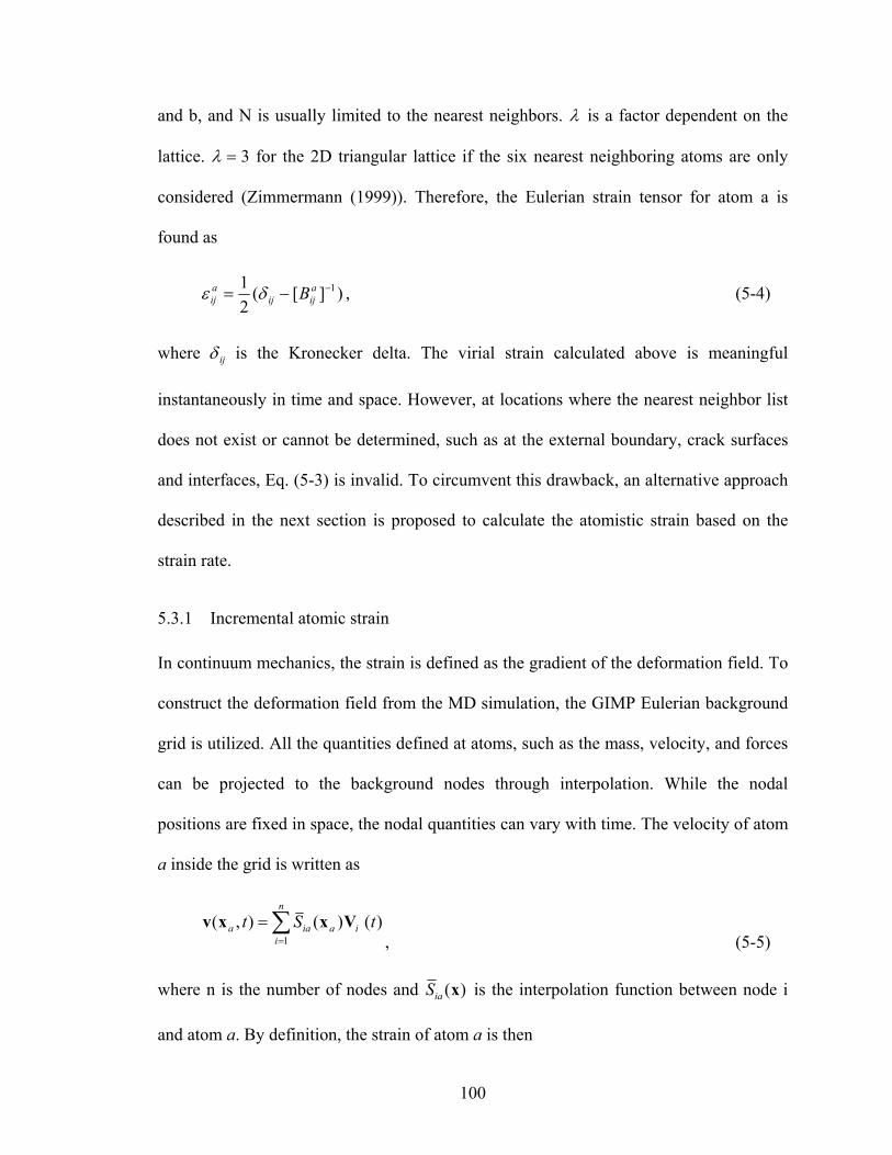
100
and b, and N is usually limited to the nearest neighbors. λ is a factor dependent on the
lattice. 3=λ for the 2D triangular lattice if the six nearest neighboring atoms are only
considered (Zimmermann (1999)). Therefore, the Eulerian strain tensor for atom a is
found as
)][(21 1−−= a
ijijaij Bδε , (5-4)
where ijδ is the Kronecker delta. The virial strain calculated above is meaningful
instantaneously in time and space. However, at locations where the nearest neighbor list
does not exist or cannot be determined, such as at the external boundary, crack surfaces
and interfaces, Eq. (5-3) is invalid. To circumvent this drawback, an alternative approach
described in the next section is proposed to calculate the atomistic strain based on the
strain rate.
5.3.1 Incremental atomic strain
In continuum mechanics, the strain is defined as the gradient of the deformation field. To
construct the deformation field from the MD simulation, the GIMP Eulerian background
grid is utilized. All the quantities defined at atoms, such as the mass, velocity, and forces
can be projected to the background nodes through interpolation. While the nodal
positions are fixed in space, the nodal quantities can vary with time. The velocity of atom
a inside the grid is written as
∑=
=n
iiaiaa tSt
1
)()(),( Vxxv, (5-5)
where n is the number of nodes and )(xiaS is the interpolation function between node i
and atom a. By definition, the strain of atom a is then

101
)],([),(21),( T
aaa ttt xuxuxε ∇+∇= , (5-6)
where ),( taxu is the deformation field. The strain rate is given by
)],([),(21),( T
aaa ttt xvxvxε ∇+∇=& . (5-7)
The velocity gradient at atom a can be expressed as ∑=
∇=∇n
aiaiaa tSt
1
)()(),( Vxxv . Using
the backward Euler time integration scheme, the strain at atom a for the next time step is
calculated through
ttta
ta
tta Δ+= Δ+Δ+ εεε & , (5-8)
where ∑=
Δ+Δ+Δ+ ∇+∇=n
iia
tti
ttiia
tta SS
1
)(21 VVε& .
The nodal mass, force, and momentum are computed from neighboring atoms
as ∑=
=n
a
taia
ti mSM
1
, ∑=
=n
a
taia
ti S
1
fF , ∑=
Δ+Δ+=n
a
tta
ttaia
ti mS
1
)( vP , respectively. The updated
nodal momentum and velocity are tti
ti
tti Δ+=Δ+ FPP and t
itt
itt
i M/Δ+Δ+ = PV .
5.3.2 Interpolation function
To ensure conservation of mass, momentum, and energy between the nodes and the
atoms, the interpolation function should satisfy partition of unity. The interpolation
function )(xiaS can be chosen to be the isoparametric shape functions used in finite
element analysis. However, the generalized interpolation functions with C1 continuity in
GIMP has shown better simulation stability when an Eulerian grid is used (Bardenhagen
and Kober (2004); Ma, Wang, Lu, Roy, Hornung, Wissink and Komanduri (2005)) and it

102
is used to compute the atomic strain in this investigation.
The generalized interpolation function introduced by Bardenhagen and Kober (2004)
consists of two functions, the nodal shape function and the particle characteristic function.
Both the nodal shape function and the material point characteristic function can be
extended to 3D. In three dimensional situations, the nodal shape function for node i is
given by
)()()()( zSySxSS zi
yi
xii =x , (5-9)
and the particle characteristic function, for a brick shaped particle p, is given by
)()()()( zyx zp
yp
xpp χχχχ =x , (5-10)
where
⎪⎪⎩
⎪⎪⎨
⎧
−≤≤−≤−−
≤−≤−−+−≤−
=
ix
xixi
ixxi
xi
xi
xxLLxxLxx
xxLLxxLxx
xS
00/)(1
0/)(10
)( , (5-11)
and
)]([)]([)( xpxpxp lxxHlxxHx +−−−−=χ , (5-12)
where H(x) denotes the step function. Fig. 5-2 shows a rectangular grid cell with a
particle in it. The particle position is taken at the center of the particle. It is noted that the
grid associated with the generalized interpolation function is a structured grid, which is
convenient to construct and process.
Both the nodal shape function and the particle characteristic function are a partition of
unity, i.e., 1)( =∑p
p xχ and 1)( =∑i
iS x . The generalized interpolation function is a

103
volume averaged weighting function between node i and material points p given by
∫Ω∩Ω
=p
dSV
S ipp
ip xxx )()(1 χ , (5-13)
where Ω is the entire computational configuration, pΩ is the spaces occupied by particle
p, and pV is the current particle volume.
Fig. 5-2: 2D representation of a particle and a grid cell
The atoms are generally regarded as spherical in shape. The characteristic function of a
sphere can also be found. However, to simplify the computation of the interpolation
function and its gradient, it is assumed that the atoms are cubic in shape with the same
volume of a spherical atom. It is also assumed that the shape and orientation of the atoms
do not change in the simulation. Consequently, Eq. (5-13) is simplified as
∫∫∫+
−
+
−
+
−
=zp
zp
yp
yp
xp
xp
lz
lz
zi
ly
ly
yi
lx
lx
xi
zyx
ip dzzSdyySdxxSlll
S )()()(8
1 . (5-14)
The final expression of the interpolation function and its gradient can be found in
Bardenhagena and Kober (2004). The interpolation function is plotted in Fig. 2-3. The
vertical axis is the interpolation function and horizontal plane is the particle position. The
node is at (0, 0). The cell size is 1×1 and the particle size is 0.5×0.5. The interpolation
Lx
Ly
(x1 ,y1) (x2 ,y2)
(xp ,yp)
2lx
2ly
(x4 ,y4) (x3 ,y3)

104
function is continuous and smooth. It may be noted that the volume bounded by the
surface of the interpolation weight and the horizontal plane is one.
-1-0.5
00.5
11.5
-1.5 -1 -0.5 0 0.5 1 1.5
0
0.2
0.4
0.6
0.8Weight
Fig. 5-3: The generalized interpolation function in 2D
5.3.3 Numerical validation
Several MD simulations are performed to calculate the atomistic strain in 2D. In these
simulations, the atomic potential chosen is the Lennard-Jones potential given by
)(4)( 6
6
12
12
0 rrrU σσε −= (5-15)
with 0.10 =ε eV and 1=σ Å. The mass of each atom is assumed to be 1 amu. The unit
time is τ = 10 fs. The potential in Eq. (5-15) gives the elastic wave speeds as follows:
longitudinal wave speed 99.8=lc Å/τ, shear wave speed 19.5=sc Å/τ, and the
Rayleigh wave speed 80.4=Rc Å/τ. A 2D triangular lattice is used in the simulations.
The model has 40 lattices in the X direction and 20 lattices in the Y direction. The size of
the model is 44×39 Å2. The atom is assumed to be cubic with a volume of unity.
The first simulation is simple tension as shown in Fig. 5-4 (a). The model is constrained
in the X direction on the left while a constant velocity is applied on two layers of lattices
on the right. The strain histories of the atom initially at (24.5, 11.2) Å calculated using the

105
virial formula and the new incremental approach are plotted in Fig. 5-5 (a). It can be seen
that in general the strains calculated from different methods agree reasonably well. The
virial strain shows more oscillations than the incremental strain. The interpolation
between the nodes and the atoms is also a spatial averaging process. Two cell sizes, 2 Å
and 2.5 Å are used in the background grid to investigate the effect of cell size. It can be
seen that oscillation of the strain are smaller when the cell size is bigger and vice versa
because the nodal quantities are interpolated from a bigger number of atoms. A large
content of noise, as a result of random thermal vibration of the atoms, has been
suppressed due to averaging over a number of atoms. For comparison, the strain from
continuum simulation, assuming the model material to be homogeneous, isotropic, and
linearly elastic using the finite element method, is also plotted. It is seen that all
simulations show that the strain first increases at time between t = 2.5 τ and 3 τ. The
calculated time is t = 2.8 τ based on the longitudinal stress wave speed.
Fig. 5-4: Two examples to calculate the atomistic strain: (a) Tension (b) Shear
The second simulation is a shearing problem as shown in Fig. 5-4 (b). Constant upward
velocity is applied on the two lattices on the right. The resultant shear strain at (24.5, 11.2)
Å is plotted in Fig. 5-5 (b) from these simulations. The virial strain again shows largest
variation, while the strain defined herein shows much less vibration.
(a) (b)
X
Y

106
Fig. 5-5: Strain histories from different simulations
Time
ε x
2 4 6 8 10 12-0.12
-0.09
-0.06
-0.03
0
0.03
0.06
Incremental-cell size=2VirialFE
Fig. 5-6: Comparison of the normal strain of a surface atom in tension
It is noted that computation of the incremental atomic strain does not depend on the
atomic potential function and the lattice structure. The deformation field is recovered at
the grid nodes using interpolation. Interpolation also allows averaging on the
displacement field so that the computed atomic strain shows less oscillation. It is known
that the virial formula is not applicable to atoms on the surface, see Zimmermann (1999).
The incremental formulation developed in this investigation, however, does not have this
restriction. The strains of the atom at the top surface (in the middle of the model) from
three computations are plotted in Fig. 5-6. It can be seen that prediction of incremental
Time
ε x
0 2 4 6 8 10 12-0.01
0
0.01
0.02
0.03
0.04
0.05Incremental-cell size=2Incremental-cell size=2.5VirialFE
(a) Tension Time
ε xy
2 4 6 8 10 12-0.01
0
0.01
0.02
0.03
Incremental-cell size=2Incremental-cell size=2.5VirialFE
(b) Shear

107
formulation is in reasonably good agreement with the finite element analysis.
The ability to compute the strains for the boundary and surface atoms is essential for
coupling simulations. For example, the strain at the crack surface is required in coupling.
It may be noted that the virial formulation computes a transient strain so that it does not
depend on the strain history. The incremental strain proposed herein is computed from
the strain rate so that it must be computed at every time increment during the entire strain
history of interest.
5.4 Coupling of GIMP and MD Simulations
5.4.1 Coupling scheme
To enable coupling between GIMP and MD, the information must be exchanged between
the atomistic simulation on one side and the continuum simulation on the other. A
successful coupling is indicated by the seamless transfer of the deformation, internal
forces, heat, etc. at the interface of two different simulation regions.
In the coupling scheme presented in this chapter, heat transfer between the continuum
and atomistic regions is neglected. Moreover, the transition region is assumed to remain
in the linear elastic regime at this stage. Fig. 5-7 (a) shows the overall coupling model
and Fig. 5-7 (b) shows details of the transition zone. The MD region covers a small
portion of the overall model and the continuum region covers the rest. The transition
region, where the communication between GIMP and MD simulations take place, is
divided into three zones, the inner zone, the “incommunicado” zone, and the outer zone,
as shown in Fig. 5-7 (b).
In the inner zone, the information is passed from MD to GIMP. The atomic strain is

108
computed using the incremental scheme presented in Sections 3.1 and 3.3. The velocity
and strain rate at the material points overlapped within the atomistic region are computed
using Eqs. (5-5) and (5-7) by replacing the atom positions with the positions of the
material points. Hence, the stresses of these points are computed based on continuum
theories. Consequently, the material points inside the atomistic region can be updated by
the atomistic information. These material points can participate in the overall continuum
computation to provide information for the rest of the continuum region. The innermost
rectangle in Fig. 5-7 (a) represents the region in which all material points are updated
based on the atomistic information. These material points are shown in Fig. 5-7 (b) as
filled squares. The unfilled squares are the material points that are updated in regular
continuum computations.
Fig. 5-7: Illustration of coupled GIMP and MD simulations. The circles represent atoms and squares (smaller than physical size) material points. The material points
connect to each other without a gap to represent continuum
The boundary atoms in the outer zone, shown as filled circles in Fig. 5-7, update their
velocities based on the interpolation with the background grid node using Eq. (5-5). The
nodal velocities of the background grid are computed from the velocities of the material
MagnifiedAtomistic
Continuum
(a) Overall regions of a model (b) Transition region with background grid
Incommunicado zone
Inner zone Outer zone

109
points weighted by the masses of the material points, as
∑
∑=
pppip
pppppip
i
S
tSt
mx
xvmxV
)(
),()()( . (5-16)
Once the velocities of the boundary atoms are known, their displacements can be found
from the time integration of the velocities. At this point, the interactions with interior
atoms are fully defined by the inter-atomic potentials as in regular molecular dynamics
simulations.
In the proposed coupling scheme, two different zones are used for communication in
different directions, i.e. from GIMP to MD or from MD to GIMP. The “incommunicado”
zone is the gap that separates the inner and outer zones. This zone serves as a buffer for
the communication between the material points and the atoms. The width of this zone is 3
to 4 layers of material points. In this coupling scheme, iteration to obtain the converged
solution in the transition zone is not necessary, as the source of information is guaranteed
to be correct and the communication in each zone is unidirectional. This approach not
only simplifies the coupling algorithm but also improves the stability and reduces the
computational cost.
The time step for MD simulation is usually smaller than the time step for GIMP, and can
be used as the time step in the coupled simulation to reach stability in coupled simulation.
However, with the use of the smaller MD time step as the overall time step in a coupled
simulation, the amount of computation is enormous. In this coupling algorithm, a
temporal coupling scheme is developed. A temporal factor N is defined as the ratio of the
GIMP time step to the MD time step; that is,
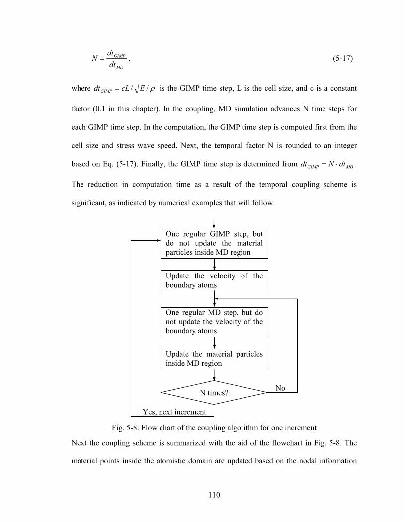
110
MD
GIMP
dtdt
N = , (5-17)
where ρ// EcLdtGIMP = is the GIMP time step, L is the cell size, and c is a constant
factor (0.1 in this chapter). In the coupling, MD simulation advances N time steps for
each GIMP time step. In the computation, the GIMP time step is computed first from the
cell size and stress wave speed. Next, the temporal factor N is rounded to an integer
based on Eq. (5-17). Finally, the GIMP time step is determined from MDGIMP dtNdt ⋅= .
The reduction in computation time as a result of the temporal coupling scheme is
significant, as indicated by numerical examples that will follow.
Fig. 5-8: Flow chart of the coupling algorithm for one increment
Next the coupling scheme is summarized with the aid of the flowchart in Fig. 5-8. The
material points inside the atomistic domain are updated based on the nodal information
One regular GIMP step, but do not update the material particles inside MD region
Update the velocity of the boundary atoms
One regular MD step, but do not update the velocity of the boundary atoms
Update the material particles inside MD region
N times? No
Yes, next increment

111
interpolated from the atoms. These material points join the GIMP calculation to provide
boundary conditions, but are not updated again. The velocity and position of the
boundary atoms are updated based on the nodal information interpolated from the
material points. These boundary atoms join the MD calculation to provide boundary
conditions as well, but the velocities are not updated. The concept of temporal coupling is
introduced by advancing the MD simulation N steps for every GIMP step, in order to
save computational time. It may be noted that the material points further inside the MD
region can be ignored to reduce the amount of computation since only a few layers of
material points are needed to provide boundary conditions to the exterior material points.
5.4.2 Parallel processing of the coupled model
The parallel processing for the GIMP with multilevel refinement using SAMRAI has
been discussed in detail in (Ma, Wang, Lu, Roy, Hornung, Wissink and Komanduri
(2005)). The coupling between GIMP and MD is performed at the finest level only. So
the finest level is always larger than the MD domain. The finest level is divided into
rectangular regions using SAMRAI “patches”. Each patch is assigned to one processor
and the communication between patches is performed after each patch is computed. To
eliminate data transferring between processors in the coupling process, the MD region is
decomposed into rectangular regions that are the same size as the patches. Each processor
thus handles the same spatial region for both GIMP and MD. Fig. 5-9 shows three levels
of refinement for GIMP with MD coupled in the finest level. The dashed lines divide the
finest level as well as the MD domain into six rectangular regions. Each region is
computed by a processor and the communication between the material points and the
atoms for coupling is performed within the processor. No data transfer between the
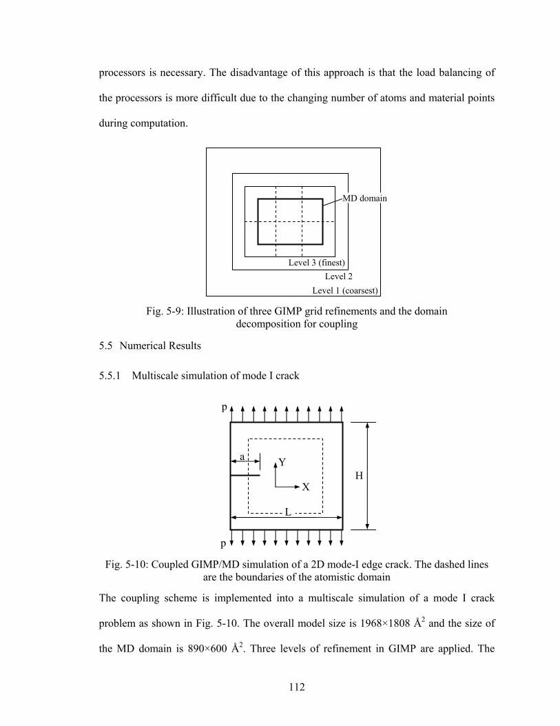
112
processors is necessary. The disadvantage of this approach is that the load balancing of
the processors is more difficult due to the changing number of atoms and material points
during computation.
Fig. 5-9: Illustration of three GIMP grid refinements and the domain decomposition for coupling
5.5 Numerical Results
5.5.1 Multiscale simulation of mode I crack
Fig. 5-10: Coupled GIMP/MD simulation of a 2D mode-I edge crack. The dashed lines are the boundaries of the atomistic domain
The coupling scheme is implemented into a multiscale simulation of a mode I crack
problem as shown in Fig. 5-10. The overall model size is 1968×1808 Å2 and the size of
the MD domain is 890×600 Å2. Three levels of refinement in GIMP are applied. The
H
a
L
p
p
X
Y
Level 1 (coarsest)Level 2
Level 3 (finest)
MD domain
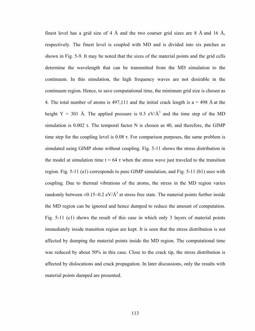
113
finest level has a grid size of 4 Å and the two coarser grid sizes are 8 Å and 16 Å,
respectively. The finest level is coupled with MD and is divided into six patches as
shown in Fig. 5-9. It may be noted that the sizes of the material points and the grid cells
determine the wavelength that can be transmitted from the MD simulation to the
continuum. In this simulation, the high frequency waves are not desirable in the
continuum region. Hence, to save computational time, the minimum grid size is chosen as
4. The total number of atoms is 497,111 and the initial crack length is a = 498 Å at the
height Y = 301 Å. The applied pressure is 0.3 eV/Å3 and the time step of the MD
simulation is 0.002 τ. The temporal factor N is chosen as 40, and therefore, the GIMP
time step for the coupling level is 0.08 τ. For comparison purposes, the same problem is
simulated using GIMP alone without coupling. Fig. 5-11 shows the stress distribution in
the model at simulation time t = 64 τ when the stress wave just traveled to the transition
region. Fig. 5-11 (a1) corresponds to pure GIMP simulation, and Fig. 5-11 (b1) uses with
coupling. Due to thermal vibrations of the atoms, the stress in the MD region varies
randomly between ±0.15~0.2 eV/Å3 at stress free state. The material points further inside
the MD region can be ignored and hence dumped to reduce the amount of computation.
Fig. 5-11 (c1) shows the result of this case in which only 3 layers of material points
immediately inside transition region are kept. It is seen that the stress distribution is not
affected by dumping the material points inside the MD region. The computational time
was reduced by about 50% in this case. Close to the crack tip, the stress distribution is
affected by dislocations and crack propagation. In later discussions, only the results with
material points dumped are presented.

114
Fig. 5-11: Stress distribution for P = 0.3 eV/Å3
Fig. 5-11 also shows the same model at time t = 112 τ. At this moment the stress
concentration at the crack tip has developed. The crack just started to open. The stress
t = 64 τ t = 112 τ
(a1) Pure GIMP (a2) Pure GIMP
(b1) Coupled (b2) Coupled
(c2) Coupled with dumping (c1) Coupled with dumping

115
fields from pure GIMP simulation and coupled simulation are shown in Fig. 5-11 (a2)
and (b2), respectively. The difference of the maximum normal stress in the Y direction is
8%. The coupling region is zoomed in and shown in Fig. 5-12, corresponding to the
region indicated by the dashed rectangle in Fig. 5-11 (c2). The material points taking
information from the atoms are overlapped inside the MD region. These material points
cannot be seen in Fig. 5-12 due to the high density of the atoms.
Fig. 5-12: Simulation model with an edge crack with P = 0.3 eV/Å3 at t = 208 τ
It is noted that the reduction of computational time due to the temporal coupling with N =
40 is about 75%, compared to the same simulation with N = 1 (no temporal coupling).
The GIMP step involves regular GIMP calculation and communication between patches
and levels (refinement and coarsening). The GIMP computation time is significantly
larger than that of an MD step in this example. Temporal coupling has reduced the
computational time significantly while maintaining the accuracy of coupling, as shown in
Fig. 5-11.
3 levels
MD

116
Time
Ene
rgy
0 60 120 180 240 300 3600
500
1000
1500
2000
2500
3000External workTotal potential energyTot energy
Fig. 5-13: Energies in the model with P = 0.15 eV/Å3
Time
Ene
rgy
Rel
ease
Rat
e
220 240 260 280 300 320 340 3600
5
10
15
20Coupled simulationCrack Resistance
Fig. 5-14: Energy release rate P = 0.15 eV/Å3
To study the energy release rate of a mode I crack using the coupling algorithm, a tensile
pressure of 0.15 eV/Å3 is applied from t = 0 to t = 210 τ. The crack started to propagate at
t = 225 τ and stopped at t = 334 τ. The external input energy, total potential energy and
total energy from the simulation are plotted in Fig. 5-13. Due to the numerical damping,
the total energy decreases as time increases. The energy loss at t = 360 τ is 20%.
Numerical simulation was conducted for this same model without damping and the
difference between the input energy and the system energy gain is less than 8%. The
potential energy is the sum of the potential energy of the atoms and the strain energy of

117
the material points. It increases at first when the model is stretched. After the crack starts
to propagate the potential energy drops. The energy release rate for this simulation is
plotted in Fig. 5-14, as well as the crack resistance. The energy release rate fluctuates as
the crack propagates and its magnitude is larger than the crack resistance. After t = 330 τ
the energy release rate drops below the crack resistance, leading the crack to arrest.
5.5.2 Multiscale simulation of mode II crack
Fig. 5-15: Boundary conditions of the mode II crack problem
The same model in Fig. 5-10 was simulated under a mode II condition by applying
velocities on the left side of the model as shown in Fig. 5-15. The applied shearing
velocities in the X direction, are -0.1 Å/τ and 0.1 Å/τ for the top half and bottom half,
respectively. Moreover, to avoid the contact of the initial crack surfaces, a velocity in the
Y direction is applied on the left boundary, 0.003 Å/τ for the top half and -0.003 Å/τ for
the bottom half. The relatively small velocity in the Y direction was applied to open crack
slightly to avoid the interaction of the crack surfaces. The initial crack is horizontal with
the tip located at (67, 301) Å. This problem was simulated with both the coupled model
and full MD model at zero temperature.
The velocities of the atoms in the X direction from the pure MD simulation are shown in
X
Y Vx
Vy

118
Fig. 5-16 (a). In this simulation, a crack was introduced to the left of the crack tip by
eliminating the interaction of the atoms on both sides of the crack. As the velocities were
applied on the boundary, the predominant deformation in the model is shearing. The path
of the shearing front was observed to be straight, as an extension to the initial crack. The
relative shearing motion between the two layers of atoms, which generate dislocations,
occurred in the stick/slip mode, as indicated by Fig. 5-16 (a). The blue spots indicate
atoms moving to the left at a velocity of ~0.7 Å/τ and relative velocity between the atoms
on the top and bottom is ~0.8 Å/τ. Between the blue spots, the relative velocity is very
small, in the range of 0 and 0.2 Å/τ. Most of the shear surfaces stick together and slip
occurs at isolated spots.
Fig. 5-16: Comparison of results from pure MD and coupled simulations at t = 11.2 τ
The results from the coupled simulation are plotted in Fig. 5-16 (b) for comparison. It can
be seen that the velocity contours agree well with pure MD simulations. The stick/slip
pattern also matches. This further verifies the accuracy of the coupling algorithm. It may
be noted that for this size of model, there are 3.3 million atoms in the pure MD
simulation, and only 0.5 million atoms and three levels of material points in the coupled
simulation. The computation time and memory for coupled simulation are 8% and 30%
(a) Pure MD (b) Coupled

119
less than the pure MD simulation, respectively. As the model grows bigger, the reduction
in both computation time and memory size will be more significant.
Fig. 5-17: Dislocation path at different simulation time
To track the dislocations in the atoms, the relative displacement of each atom with
respect to each neighboring atom was computed and the maximum relative displacement
was recorded for the atom. Fig. 5-17 plots the maximum relative displacement of the
atoms at different simulation times when the cut-off value of the maximum relative
displacement is set to 0.15 Å; i.e., atoms with maximum relative displacement of less
than or equal to 0.15 Å are not shown. With this cut off value, all the visible atoms are
those immediately on two sides of the crack extension and those with the stick/slip
pattern. The left end of each plot is the crack tip and right end is the slip front. The
average propagation speed of the slip frontier is ~3.5 Å/τ during t = 64 τ and t = 160 τ.
5.6 Conclusions
A coupled atomistic/continuum simulation method is presented by coupling MD
simulations with GIMP simulations. To enable coupling, a method for the computation of
atomistic strain, based on the computation of strain rate, is developed. The atomic strain
rate is computed by first interpolating the velocities of the atoms to a background
t=64 τ t=80
t=96 t=112
t=128
t=144
t=160

120
Eulerian grid, then computing the gradient of grid velocities. The computed atomic strain
shows less vibration than that computed by the virial theorem due to noise reduction in
the interpolation process. The generalized interpolation function is chosen as the
interpolation function for GIMP and a structured grid is used for the background grid.
The atomic stress is then computed based on strain using the isotropic and homogeneous
constitutive law.
The coupling algorithm uses a common background grid for MD and GIMP. The
velocities of the boundary atoms are computed from the grid velocities, which are
interpolated from the material points. The material points inside the MD region are
updated based on the atomic information and these points join the rest of the material
points in the GIMP computation. This approach ensures the compatibility of deformation
and internal forces at the MD/GIMP interface region.
A multi-level refinement scheme for GIMP is used to refine the material points close to
the atomistic size. The coupling algorithm is implemented using the SAMRAI
(Structured Adaptive Mesh Refinement Application Infrastructure) for parallel processing.
The finest GIMP level is coupled with the MD simulation. The MD region is
decomposed into domains with the same geometry as the GIMP patches. Each patch is
assigned to a processor and the coupling between the atoms and material points is
performed inside each processor without extra inter-processor communication.
The coupling algorithm was verified by comparing the coupling results with the pure
GIMP and with the pure MD simulations. A mode I crack propagation problem was
simulated using the proposed the coupling technique. The stress field of the coupled
model is verified by comparison with pure GIMP simulations in the elastic stage. The

121
energy release rate is computed and it is found that the crack arrests after the energy
release rate is less than the crack resistance. In mode II loading, stick/slip was observed
in the crack front and the results compared well with pure MD simulation. While the
current implementation is in 2D, the coupling algorithm can be applied to 3D.
The coupling algorithm presented here can be extended to include discrete dynamics
outlined in the CADD method (Curtin and Miller (2003); Shiari, Miller and Curtin
(2005)). A dislocation detection band can be placed inside the inner zone in Fig. 5-7
which in turn can be fed into the continuum region, and vice versa.

122
Chapter 6
Multiscale Simulation of Nanoindentation using GIMP, Dislocations Dynamics and
Molecular Dynamics
A multiscale simulation technique coupling three scales, i.e., the molecular dynamics
(MD) at the atomistic scale, the discrete dislocations at the meso scale and the
generalized interpolation material point (GIMP) method at the continuum scale, is
presented. Discrete dislocations are first coupled with GIMP using the principle of
superposition (van der Giessen and Needleman (1995)). A detection band seeded in the
MD region is used to pass the dislocations to and from the MD simulations (Shilkrot,
Miller and Curtin (2002)). A common domain decomposition scheme for each of the
three scales was implemented for parallel processing. Simulations of indentation were
performed on the (111) plane of Cu at 0 °K indented by a cylindrical indenter. The effects
of indenter radius, indentation speed on the indentation load-depth curve and dislocations
were studied. For simulations at finite temperatures, temperature rescaling technique was
used to rescale the atom velocities in the MD region to maintain a constant temperature.
Simulations were also performed at different temperatures to determine the effect of
temperature.
6.1 Introduction
Multiscale modeling has received increasing attention in modeling material behaviors in
recent years due to its capability to simulate and link physical events occurring at various

123
length and temporal scales. At the atomic scale, simulation techniques based on atom
motion, such as molecular dynamics and Monte Carlo simulations can reveal the
fundamental aspects on material deformation provided that the amount of computation is
accommodated by the current computing power. At larger scales where atomistic
simulation cannot be readily applied due to excessive computing cost, techniques such as
discrete dislocation dynamics at the mesoscopic level and finite element analysis at the
macroscopic level have been employed. With appropriate coupling techniques,
simulation at different scales can be bridged to obtain the most accurate information in
areas where atomistic revolution is desired while allowing the dislocation and continuum
descriptions to model the material behaviors in areas farther away without the significant
loss of accuracy.
Several techniques have been proposed for simulations bridging two or more scales
(Kohlhoff, Gumbsch and Fischmeister (1991); Shilkrot, Miller and Curtin (2002); Curtin
and Miller (2003); Shiari, Miller and Curtin (2005); Raffi-Tabar, Hua and Cross (1998)).
At each individual scale, simulation techniques have been well established. However, the
treatment on transition region, or handshake region, overlapped by the outer boundary of
the atomistic region and the inner boundary of the continuum region, is where the
difficulties arise (Kohlhoff, Gumbsch and Fischmeister (1991); Shilkrot, Miller and
Curtin (2002); Curtin and Miller (2003)). For example, in multiscale simulation, the finite
element method (FEM) is often used at the continuum level. However, spurious effects
can occur when waves with the wavelength larger than the element size is transmitted
from the MD region into the continuum region, and waves with wavelength smaller than
the element size are reflected artificially (Raffi-Tabbar, Hua and Cross (1998)), causing

124
artificial overheating in the MD region. Efforts were made to minimize the wave
reflection while enforcing the displacement and force continuity, as well as energy
conservation in the handshake region. Cai et al. proposed the Green’s function method
(Cai, de Koning, Bulatov and Yip (2000)) in dynamic coupling between the two regions
and this technique shows advantages in minimizing wave reflection. A multi-scale
framework merging two scales, the microscale and the continuum scale was developed to
create a hybrid elasto-viscoplastic simulation model coupling discrete dislocation
dynamics with finite element analysis based on the superposition principle (Zbib and
Diaz de la Rubia (2002)). At intermediate scale, the dislocation modeling was used in
bridging the continuum and atomistic simulations (Raffi-Tabar, Hua and Cross (1998)).
The involvement of dislocation dynamics in connecting the atomistic and continuum
scales enables the model to handle plastic deformation through the explicit motion of
dislocation defects in the continuum region. With this feature, the multiscale model is
completely structured for applications such as nanoindentation (Shiari, Miller and Curtin
(2005)).
Plastic deformation in crystalline metals is the result of motion of large numbers of
dislocations. Various discrete dislocation (DD) models have been developed in the past
two decades, and dislocations are usually described as line singularities in an elastic
medium (Amodeo and Ghoniem (1990); Gulluoglu and Hartley (1993); Kubin and
Canova (1992); Fang and Dahl (1993); Groma and Pawley (1993); van der Giessen and
Needleman (1995); Zbib, Rhee and Hirth (1998)). On the interactions of the dislocations,
the long-range forces are well-represented by the linear elastic fields outside a dislocation
core radius of about five Burgers vectors from a dislocation. Within a distance of several

125
Burgers vectors from the core, the displacement field around the dislocation is nonlinear
and cannot be described accurately by linear elasticity (Amodeo and Ghoniem (1990)).
Instead, a set of constitutive rules were used to represent the short range interactions
between dislocations. Recently, nonlinear deformation has been considered in coupling to
represent the physical phenomenon. The coupled atomistic/continuum discrete
dislocation (CADD) method has demonstrated its capability in detecting dislocations in
the atomistic region and converting the atomistic dislocations into discrete dislocations in
the continuum region (Shilkrot, Miller and Curtin (2004)). A dynamic version of the
CADD method has been used to study the nanoindentation process as a function of
temperature and rate of indentation (Shiari, Miller and Curtin (2005)).
While FEM has been developed as an appealing simulation technique at the continuum
scale, it is subjected to some difficulties, including the complexity in mesh generation for
computational bodies with complex geometries and severe mesh distortion under large
nonlinear deformations. To overcome some of the limitations of FEM, the material point
method (MPM) (Sulsky, Zhou and Schreyer (1995); Sulsky and Schreyer (1996)) was
introduced for dynamic simulations and the general interpolation material point (GIMP)
method (Bardenhagen and Kober (2004)) was presented with improved simulation
stability. In these methods, material points that can conform to the geometry complexity
with ease are used to discretize the computational body. Further, these methods can avoid
the mesh entanglement problem because of the use of Lagrangian description for material
points carrying physical quantities and the use of Eulerian description for convection of
physical variables and solution of field equations. A new method for multiscale
simulation bridging two scales, namely, the continuum scale using the GIMP method and
126
the atomistic scale using MD was proposed and verified in 2D, using the multilevel
refinement technique in a parallel computing environment (Ma, Wang, Lu, Roy, Hornung,
Wissink and Komanduri (2005); Ma, Lu, Wang, Hornung, Wissink and Komanduri
(2005)). Coupling between GIMP and MD is achieved by using compatible deformation,
force, and energy fields in the transition region between GIMP and MD. This coupling
framework can overcome some inherent limitations of FEM, while maintaining the
advantages of the multiscale modeling with a scheme for time-saving in parallel
computing.
In this chapter, we present a multiscale simulation scheme, encompassing GIMP at the
continuum scale, MD at the atomistic scale and DD at the mesoscale to link GIMP and
MD. The technique has expanded the previous GIMP and MD coupling method (Ma, Lu,
Wang, Hornung, Wissink and Komanduri (2005)), to introduce discrete dislocations in
the framework of coupling. Dislocation accommodation and propogation mechanisms are
introduced by detecting dislocations through the MD simulation in real time and then
passing them through the boundary. This helps to alleviate the artificial wave propagation
problem in direct GIMP and MD coupling. The new method can handle larger numerical
model without drastically increase the computational expense, as the introduction of DD
allows some regions previously modeled by MD to be simulated by DD. DD can
substitute MD in simulating some of the critical areas without significant loss of accuracy
and the computation is more economical for the same model.
6.2 Coupling Scheme between GIMP, DD and MD
6.2.1 Coupling of GIMP and MD
In this section, we review briefly an algorithm that couples the continuum and atomistic

127
scales directly. At the continuum scale, the generalized interpolation material point
(GIMP) method is used. Fig. 6-1 illustrates the coupling scheme in which the atomistic
region is embedded in the continuum region as shown in Fig. 6-1 (a). A transition region,
where the communication between the two regions takes place, is constructed by
overlapping the material points and the atoms by certain width, as shown in Fig. 6-1 (b).
A common background grid is used to carry out the communication by interpolating the
physical quantities, such as the velocity and forces, back and forth between the
continuum region and the atomistic region. The material points in the inner zone, shown
in Fig. 6-1 (b), are updated from atomistic simulation, and then join the rest of the
material points in the GIMP simulation. The velocities of the atoms in the outer zone are
updated by the continuum region, and then provide boundary conditions for the MD
simulation.
Fig. 6-1: Illustration of coupled GIMP and MD simulations. The circles represent atoms and squares (smaller than physical size) material points. The material points connect to
each other without a gap to represent continuum
Refinement algorithms in GIMP have been developed to split the material points to the
size of atoms at the transition region to achieve seamless coupling. However, if
MagnifiedAtomistic
Continuum
(a) Overall regions of a model (b) Transition region with background grid
Incommunicado zone
Inner zone Outer zone
Transition

128
dislocations cannot be modeled explicitly in the continuum region, the atomistic region
has to be large enough so that the dislocations do not propagate to the transition region,
i.e., the continuum region remains elastic.
6.2.2 Bridging the continuum and atomistic scales with DD
In order to detect dislocations when they are generated in the MD region and then pass
them into the continuum region, the method for dislocation detection and passing
algorithm proposed by Shilkrot, Miller and Curtin (2004) was implemented into the
GIMP and MD coupling. Several layers of atoms at the border of the MD region and the
continuum region form detection band elements, which are triangular in shape. During
deformation, the Lagrangian strain tensor of an element in the detection band is
][21 IFFE −= T (6-1)
where F is the deformation gradient tensor and it is decomposed into
peFFF = . (6-2)
In Eq. (6-2), eF is related to the lattice stretching while pF corresponds to the plastic
shearing of the slip systems of the crystal. For the case of ideal slip deformation, IF =e .
And pF can be represented by:
⎟⎠⎞
⎜⎝⎛ ⊗+=
dp mbIRF , (6-3)
where R is the lattice rotation and d is the interplanar distance, b and m are the
Burger’s vector and the normal of the slip plane, respectively. Substituting Eq. (6-3) into
Eq.( 6-1) , we get the plastic slip strain tensor as
=−= ])[(21 IFFE Tpp
22))(()(
ddsym mbbmmb ⊗⊗
+⊗
(6-4)
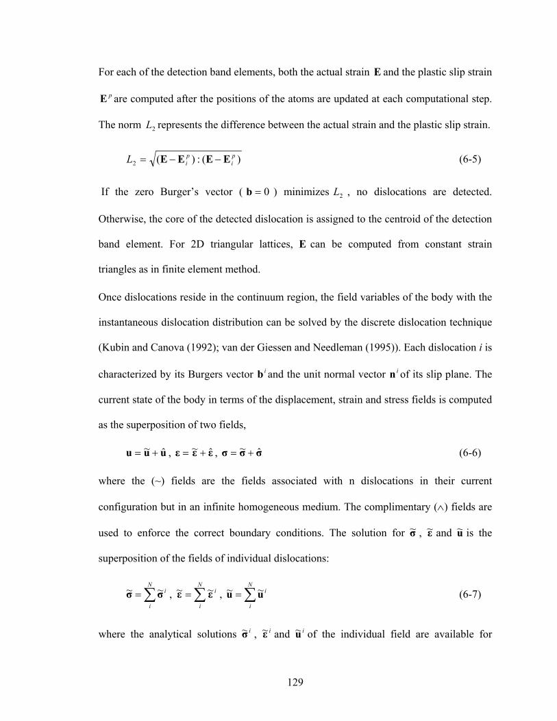
129
For each of the detection band elements, both the actual strain E and the plastic slip strain
pE are computed after the positions of the atoms are updated at each computational step.
The norm 2L represents the difference between the actual strain and the plastic slip strain.
)(:)(2pi
piL EEEE −−= (6-5)
If the zero Burger’s vector ( 0=b ) minimizes 2L , no dislocations are detected.
Otherwise, the core of the detected dislocation is assigned to the centroid of the detection
band element. For 2D triangular lattices, E can be computed from constant strain
triangles as in finite element method.
Once dislocations reside in the continuum region, the field variables of the body with the
instantaneous dislocation distribution can be solved by the discrete dislocation technique
(Kubin and Canova (1992); van der Giessen and Needleman (1995)). Each dislocation i is
characterized by its Burgers vector ib and the unit normal vector in of its slip plane. The
current state of the body in terms of the displacement, strain and stress fields is computed
as the superposition of two fields,
uuu ˆ~ += , εεε ˆ~ += , σσσ ˆ~ += (6-6)
where the (~) fields are the fields associated with n dislocations in their current
configuration but in an infinite homogeneous medium. The complimentary (∧) fields are
used to enforce the correct boundary conditions. The solution for σ~ , ε~ and u~ is the
superposition of the fields of individual dislocations:
∑=N
i
iσσ ~~ , ∑=N
i
iεε ~~ , ∑=N
i
iuu ~~ (6-7)
where the analytical solutions iσ~ , iε~ and iu~ of the individual field are available for

130
straight dislocations in 2D stress state in an infinitely large isotropic material (Hirth and
Lothe (1982)).
On the update of dislocations, the Peach-Koehler (P-K) force ip is the driving force for
evolvement in the dislocation topology and it is computed by
iN
ij
Tiip bσσn ⋅+⋅= ∑≠
)~ˆ()( . (6-8)
Using the linear drag relation, the magnitude of the glide velocity of dislocation iv is
computed from the Peach-Koehler force through
ii Bvp = , (6-9)
where B is the drag coefficient. Then each dislocation i is displaced by tviΔ , followed by
the determination of the stress and strain state for the updated dislocation structure.
6.2.3 Parallel processing
The parallel processing scheme for coupling GIMP with MD has been developed using
domain decomposition for both MD and GIMP in Chapter 5. It is noted that only the
finest level of GIMP is coupled with MD. For all the coarser levels, pure GIMP
calculation is carried out. When the discrete dislocation is incorporated into the coupling
algorithm, care must be taken in the multi processor distributed processing. The DD
algorithm shows that the amount of DD related computation is proportional to 2DN ,
where DN is the number of dislocations. In this investigation, the computational cost of
DD is much less than that of MD and GIMP. Hence, we still adopt the same physical
domain decomposition as in GIMP for DD as describe in Chapter 5. Fig. 6-2 shows a
schematic of an indentation problem in the coupling simulation. The area immediately

131
beneath the indenter is modeled by MD. Three levels of successive refinements in GIMP
are shown with the finest level decomposed into six rectangular patches. Other levels are
also divided into 6 patches and these patches are not shown. Even though using the same
domain decomposition for MD and GIMP in the finest level does not produce the best
load balance among the processors, this approach is simple to implement and effective in
the communication between GIMP and MD in the transition region, because material
points and atoms in exchange of information are stored and processed by the same
processor, and hence, no inter-processor communication is necessary.
Fig. 6-2: Illustration of the domain decomposition and refinement for the coupling simulation of 2D indentation using GIMP, DD and MD
When discrete dislocations, shown as small squares in Fig. 6-2, are introduced into the
model, we keep the domain decomposition intact. Fig. 6-3 shows the overall flowchart of
the coupling algorithm incorporating GIMP, DD and MD. Each DD is updated within
each patch where it resides because the local continuum stress is needed to compute the
Peach-Koehler force applied on it. Because the long-range forces from all other DDs
have to be computed, i.e., loop all the DDs, we store the updated information of all the
DD’s in each processor. Hence, inter-processor communication can be avoided. The cost
Level 2
Level 3
MD
Level 1 (
DDIndenter

132
is that after each step, i.e., after all patches in each level and the DDs are updated, the
updated DD information has to be broadcasted to other processors. To achieve this, each
processor sends first the local updated DD information, including newly created DDs, to
one master node and the master node assembles all the updated dislocations. Next, the
master node broadcasts all the dislocation information to all other processors. It may be
noted that each dislocation carries a position and a Burger’s vector (4 double variables in
2D) and the communication overhead is usually negligible comparing to the GIMP and
MD computations.
Fig. 6-3: Flow chart of the coupling algorithm for each increment
Update the velocities of the boundary atoms
One regular MD step, but do not update the velocities of the boundary atoms
Update the material particles inside MD region and detect new dislocations
No
Yes, next increment
Communicate and update DD in each node
Recursively advance each GIMP patch in each level; in the meanwhile, update DD; but do not update the material particles inside the MD region
N times?

133
6.2.4 Contact solver for MD
The contact algorithm to determine the contact force for each atom that penetrates into
the rigid indenter is more straightforward than the contact algorithm at the continuum
scale. A repulsive potential between the indenter and the atoms in contact can be defined
as a function of the penetration depth in the form nK |||| d⋅=Φ , where d is the
penetration depth, K is a constant that controls the strength of the repulsive potential. The
exponent n was chosen as 3 in Klchner, Plimpton and Hamilton (1998) and it was 2 in
Miller, Shilkrot and Curtin (2004). In this approach, the magnitude of K is usually
determined numerically to achieve both simulation stability and contact compatibility.
Eventually, a range of magnitudes can be used for K and convergence becomes the
decisive issue. Extra numerical experiments have to be performed to narrow the range of
K.
In this research, we avoid using the above approach by explicitly solving for the contact
force on each atom in contact by considering the penetration depth and the acceleration.
The penetration depth d can be first determined from the atom location and velocity
assuming no contact. If there is penetration, it must be eliminated during the time
increment tΔ . From 2
21 tΔ= ad , where a is the acceleration, one can determine the
contact force 22t
mm aac Δ=⋅=
daF , where am is the mass of the atom. The contact force
can then be decomposed into three components in the Cartesian coordinates based on the
local outward normal of the indenter surface.
6.3 Simulation of Nanoindentation
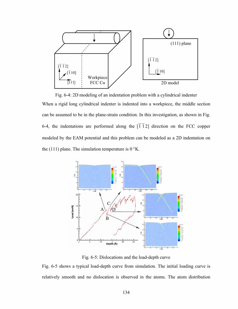
134
Fig. 6-4: 2D modeling of an indentation problem with a cylindrical indenter
When a rigid long cylindrical indenter is indented into a workpiece, the middle section
can be assumed to be in the plane-strain condition. In this investigation, as shown in Fig.
6-4, the indentations are performed along the ]211[ direction on the FCC copper
modeled by the EAM potential and this problem can be modeled as a 2D indentation on
the (111) plane. The simulation temperature is 0 °K.
Fig. 6-5: Dislocations and the load-depth curve
Fig. 6-5 shows a typical load-depth curve from simulation. The initial loading curve is
relatively smooth and no dislocation is observed in the atoms. The atom distribution
A
B
D C
Workpiece FCC Cu 2D model
]101[
]211[
]111[
]101[
]211[
(111) plane
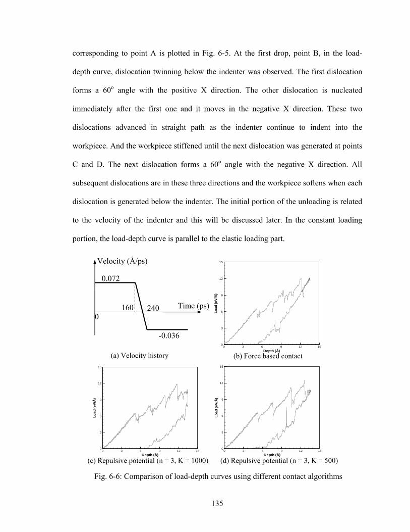
135
corresponding to point A is plotted in Fig. 6-5. At the first drop, point B, in the load-
depth curve, dislocation twinning below the indenter was observed. The first dislocation
forms a 60o angle with the positive X direction. The other dislocation is nucleated
immediately after the first one and it moves in the negative X direction. These two
dislocations advanced in straight path as the indenter continue to indent into the
workpiece. And the workpiece stiffened until the next dislocation was generated at points
C and D. The next dislocation forms a 60o angle with the negative X direction. All
subsequent dislocations are in these three directions and the workpiece softens when each
dislocation is generated below the indenter. The initial portion of the unloading is related
to the velocity of the indenter and this will be discussed later. In the constant loading
portion, the load-depth curve is parallel to the elastic loading part.
Fig. 6-6: Comparison of load-depth curves using different contact algorithms
Time (ps)
Velocity (Å/ps)
0.072
-0.036
160 240 0
Depth (Å)
Load
(eV
/Å)
0 3 6 9 12 150
3
6
9
12
15
Depth (Å)
Load
(eV
/Å)
0 3 6 9 12 150
3
6
9
12
15
Depth (Å)
Load
(eV
/Å)
0 3 6 9 12 150
3
6
9
12
15
(a) Velocity history (b) Force based contact
(c) Repulsive potential (n = 3, K = 1000) (d) Repulsive potential (n = 3, K = 500)

136
The next numerical example is to validate the force based contact algorithm by
comparing with the results from the contact pressure based contact algorithm (Klchner,
Plimpton and Hamilton (1998)). The velocity history of the rigid indenter is shown in Fig.
6-6 (a). The load-depth curves from three simulations with different contact conditions
are shown in Fig. 6-6 (b), (c) and (d), respectively. All three simulations give similar load
magnitudes and dislocation patterns. When the repulsive contact potential is used, the
loading curve appears to be smoother for K = 500 than for K = 1000. The initial portions
of the unloading curves are quite different when K is different. For this reason, the
contact force based algorithm is used in the next simulations.
Fig. 6-7: Effect of the indentation velocity on the load-depth curve
To investigate the effect of indentation velocity, simulations are performed with several
indentation velocities with a fixed indenter radius. The overall workpiece size is also
fixed at 86.8 nm ×57.8 nm. The size of the MD region is 28.9 nm ×21.7 nm. The MD
time step is 2 fs (1 fs = 10-15 s) and the temporal refinement factor is 5, i.e., the GIMP
time step is 10 fs. First, an indenter with a radius of 3.6 nm is used in the simulations of
three indentation velocities, 7.2 m/s, 36 m/s and 72 m/s. Fig. 6-7 (a) shows the
Depth (Å)
Load
(ev/
Å)
0 5 10 15 20 25 300
10
20
30
40
50
R=3.6nm V=7.2m/sR=3.6nm V=36m/sR=3.6nm V=72m/s
(a) R = 3.6 nmDepth (Å)
Load
(ev/
Å)
0 10 20 30 40 500
20
40
60
80
100
R=7.2nm V=1.8m/sR=7.2nm V=7.2m/sR=7.2nm V=36m/sR=7.2nm V=72m/s
(b) R = 7.2 nm

137
indentation load-depth curves. It is seen that the indentation load is higher if the
indentation velocity is higher at fixed depth of indentation. Another observation is that
the indentation depth at the onset of the first slippage in the workpiece is larger if the
indentation speed is lower. When the indentation speed is lower, the deformation can
propagate further so that there is less strain gradient in the workpiece. The same
phenomena are observed for these three indentation velocities when the indenter radius is
changed to 7.2 nm. However, if the indentation speed is further reduced to 1.8 m/s, the
load-depth curve is almost identical to the one with the indentation speed of 7.2 m/s, as
shown in Fig. 6-7 (b). This indicates a quasi-static condition has been reached and the
load-depth curve is converged.
Depth (Å)
Load
(ev/
Å)
0 10 20 30 40 500
20
40
60
80
100
R=1.8nm V=72m/sR=3.6nm V=72m/sR=7.2nm V=72m/s
Fig. 6-8: Effect of the indenter size on the load-depth curve
Fig. 6-8 shows three load-depth curves for three different indenter radii when the
indentation was fixed at 72 m/s. The size of the workpiece is the same as the one used in
Fig. 6-7. In this case, there is a strong dependence on the indenter size. The slope of the
load-depth curves in the elastic region increases with the increase of indenter radius.
In the theory of elasticity, assuming that the workpiece is an infinite half space, the

138
relation between indentation load P, depth h and indenter radius R is given as (Gladwell
(1980))
⎥⎦
⎤⎢⎣
⎡−=
RhhCP
2
21 , (6-10)
where C is a constant depending on the material properties only. It is seen that when the
indentation depth h is much smaller than the indenter radius R, the indentation load P is
linearly dependent on h. To investigate the effect of the workpiece boundaries on the
simulation, the indenter radius and the workpiece size are changed simultaneously so that
their ratio is a constant. Under this circumstance, each simulation would experience
relatively the same amount of boundary effect. Fig. 6-9 shows the results for three
indenter radii, 3.6 nm, 7.2 nm and 14.4 nm, when the indentation velocity is fixed at 72
m/s. It is seen that the slopes for the three curves are the same before slippage occurs,
which is consistent with the predictions in elasticity.
Depth (Å)
Load
(eV
/Å)
0 10 20 30 40 50 600
30
60
90
120
150
180
R=3.6nm V=72m/sR=7.2nm V=72m/sR=14.4nm V=72m/s
Fig. 6-9: Load-depth curves when the ratio between the workpiece size and the indenter radius is constant

139
Depth (Å)
Load
(eV
/Å)
0 10 20 30 40 500
20
40
60
80
100
120
MD R=7.2nm V=72m/sCoupled R=7.2nm V=72m/s
Fig. 6-10: Comparison of the load-depth curves between the coupling and purely MD simulations
To further validate the coupling model, a pure MD simulation was performed with the
indenter radius of 7.2 nm. A reasonably good agreement between the coupling and the
purely MD simulation can be seen from the load-depth curves in Fig. 6-10.
Fig. 6-11: Slip bands, discrete dislocations and stress distributions in the model
As discussed in previous sections, the load-depth curves drop when the dislocation is
generated below the indenter. Despite the different indenter radii and indentation
velocities used, the slip patterns are similar in the model. Fig. 6-11 shows the overall
X, Å
Y,Å
-200 0 200 400 600
-200
0
200
σy
0.005-0.01-0.025
Indenter
GIMP
MD
DiscreteDislocaitons
Slip band
Finest level
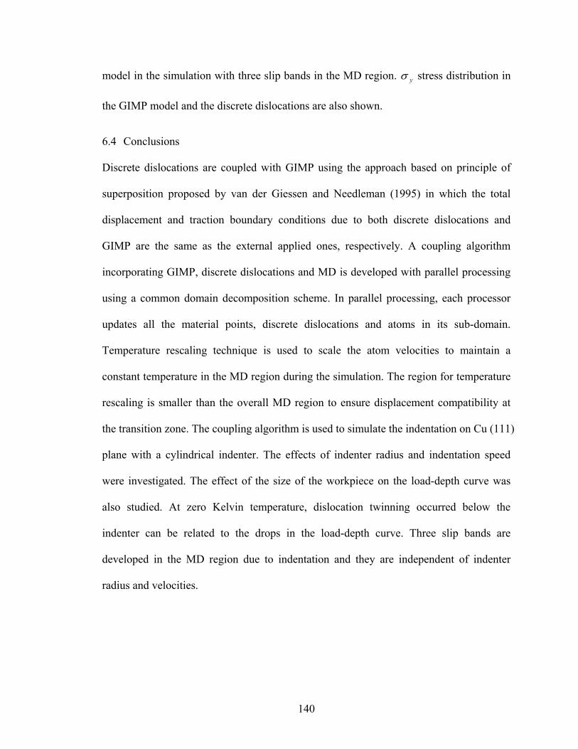
140
model in the simulation with three slip bands in the MD region. yσ stress distribution in
the GIMP model and the discrete dislocations are also shown.
6.4 Conclusions
Discrete dislocations are coupled with GIMP using the approach based on principle of
superposition proposed by van der Giessen and Needleman (1995) in which the total
displacement and traction boundary conditions due to both discrete dislocations and
GIMP are the same as the external applied ones, respectively. A coupling algorithm
incorporating GIMP, discrete dislocations and MD is developed with parallel processing
using a common domain decomposition scheme. In parallel processing, each processor
updates all the material points, discrete dislocations and atoms in its sub-domain.
Temperature rescaling technique is used to scale the atom velocities to maintain a
constant temperature in the MD region during the simulation. The region for temperature
rescaling is smaller than the overall MD region to ensure displacement compatibility at
the transition zone. The coupling algorithm is used to simulate the indentation on Cu (111)
plane with a cylindrical indenter. The effects of indenter radius and indentation speed
were investigated. The effect of the size of the workpiece on the load-depth curve was
also studied. At zero Kelvin temperature, dislocation twinning occurred below the
indenter can be related to the drops in the load-depth curve. Three slip bands are
developed in the MD region due to indentation and they are independent of indenter
radius and velocities.
141
Chapter 7
Summary and Future Work
7.1 Summary
Multiscale simulation algorithms that allow refinements from macroscale to tens of
nanometer scale at the continuum level, coupled with parallel processing have been
developed. A 2D generalized interpolation material point (GIMP) method has been
implemented to address problems, such as particle flying-off and alternating stress sign
associated with conventional material point method (MPM) in case of relatively large
deformation when material points just cross the borders of cells. For simulations at
multiple length scales, a parallel computing scheme has been implemented using GIMP
under SAMRAI parallel computing environment in which multi-level grids are used for
both spatial and temporal refinements.
Another approach for spatial refinement called structured mesh refinement using a
structured grid was developed by adding transitional nodes and by changing the influence
zone of the transition nodes in GIMP. The influence zone is square for uniform grid
nodes and rectangular for transitional nodes. The influence zone affects the computation
of the nodal shape functions. The way the weighting function is computed remains the
same as with the use of a uniform grid. The refinement scheme can be readily applied
successively and the refined grid remains structured in each refinement level, i.e., every
node can be determined by the extent of the grid level and cell size.

142
The GIMP algorithm has been extended to account for displacement boundary conditions,
based on the approach used in the meshless local Petrov-Galerkin (MLPG) method by
Atluri and Zhu (2000). A method to track the material particle deformation was
developed and validated. This method tracks the displacement of each corner of a
material particle. Since neighboring particles share corners, no separation would occur
during deformation using this approach.
Based on the effective refinement algorithm at the continuum scale, a coupled
atomistic/continuum simulation method has been developed through coupling MD
simulations with GIMP simulations. To enable the coupling, a method for the
computation of atomistic strains, based on the integration of strain rate, is developed. The
coupling algorithm uses a common background grid for MD and GIMP. The velocities of
the boundary atoms are computed from the grid velocities, which are interpolated from
the material points. The material points inside the MD region are updated based on the
atomic information and these points join the rest of the material points in the GIMP
computation. This approach ensures the compatibility of both deformations and internal
forces at the MD/GIMP handshake region.
A multi-level refinement scheme for GIMP has been used to refine the material points
multiple times until they are close to the atomistic size. The coupling algorithm is
implemented in the Structured Adaptive Mesh Refinement Application Infrastructure
(SAMRAI) for parallel processing. The finest GIMP level is then coupled with the MD
simulations. The MD region is decomposed into domains with the same geometry as the
GIMP patches. Each patch is assigned to a processor and the coupling between the atoms
and material points is performed within each processor without extra inter-processor

143
communication. The coupling algorithm was validated by comparing results from
coupled simulations with those from GIMP simulations, and also with those from pure
MD simulations. While the current implementation is in 2D, the coupling algorithm can
be applied to 3D.
Discrete dislocations are coupled with GIMP using the principle of superposition as
developed by van der Giessen and Needleman (1995) by equating the total displacement
and traction boundary conditions due to discrete dislocations and GIMP to the external
applied ones. Then a coupling algorithm incorporating GIMP, discrete dislocations and
MD is developed with parallel processing using a common domain decomposition
scheme. In parallel processing, each processor updates all the material points, discrete
dislocations and atoms in its sub-domain. The coupling algorithm has been used to
simulate the indentation on Cu (111) plane with a cylindrical indenter. The effects of
indenter radius, indentation speed, workpiece size and temperature on the
nanoindentation load-displacement curves and hardness were investigated. At zero
Kelvin temperature, the slips below the indenter is associated with the drops in the load-
depth curve. Three slip bands are developed in the MD region due to nanoindentation and
they are independent of indenter radius and velocities.
7.2 Future Work
7.2.1 Other multiscale problems
Nanostructures and nanomechanics are of critical importance in understanding material
behavior and material processing. Multiscale simulations allow simulations across
different length and temporal scales. Simulations for other problems, such as frictional
sliding and 3D indentation, using the multiscale simulation algorithm can be also

144
performed. Experimental investigations at micro/nanoscales would provide validations to
the algorithms.
Thermal coupling between the atomistic and continuum regions is necessary as most
materials are used at a temperature higher than zero absolute temperature. For problems
involving significant temperature changes, such as micro-machining, thermal coupling
has to be addressed properly in order to obtain valid results. The multiscale simulation
algorithms can be extended to include other scales, such as the tight binding (TB).
7.2.2 Simulation of metal cutting using GIMP
The other problem for which GIMP can simulate with ease is metal cutting. Metal cutting
is a complicated process which generally involves large deformation, contact, friction,
heat generation and material failure. It has been an active research area for FEM for many
years. Commercial FEM software is available for certain types of metal cutting problems
(Third Wave Systems, Inc., 2006). When GIMP is used to simulate metal cutting
problems, difficulties in FEM associated with large deformation and adaptive refinement,
material removal (element deletion) due to failure can be partially or fully eliminated.
Simulation of metal cutting problem involves issues such as contact, large deformation,
friction and heat generation, material failure, adaptive refinement, as well as material
constitutive behavior. All these aspects have been investigated except that the contact is
assumed to be frictionless.
7.2.2.1 Material model
The strain rate dependent Johnson-Cook hardening model (Johnson and Cook (1983);
Johnson and Cook (1985)) is defined as
)(0 plyy R εσσ &= , (7-1)

145
where 0yσ is the static yield stress given by
[ ] )ˆ1()(0mn
ply BA θεσ −+= , (7-2)
and )( plR ε& is the ratio of the yield stress at nonzero strain rate to the static yield stress.
plε is the equivalent plastic strain and A, B, n and m are material parameters measured at
or below the transition temperature, tθ . θ is the nondimensional temperature defined as
)()(
)(
1)/()(
0ˆ
melt
meltt
t
tmeltt
θθθθθ
θθθθθθθ
>≤≤
<
⎪⎩
⎪⎨
⎧−−= , (7-3)
where meltθ is the melting temperature. The equivalent plastic strain rate plε& is given by
00 )1(1exp yypl ifRC
σσεε ≥⎥⎦⎤
⎢⎣⎡ −= && , (7-4)
where 0ε& and C are material parameters measured at or below the transition temperature.
Hence, )( plR ε& can be found as
)ln(1)(0ε
εε
&
&& pl
pl CR += , (7-5)
and 1)( 0 =ε&R .
The Johnson-Cook shear failure model can be used in conjunction with the Johnson-Cook
plasticity model to define shear failure of the material in metal cutting. The Johnson-
Cook shear failure model is based on the value of the equivalent plastic strain at element
integration points in finite element analysis. Failure is assumed to occur when the damage
parameter exceeds one. In GIMP, it is natural to assume that the Johnson-Cook shear

146
failure model is evaluated at the material points. The damage parameter, ϖ , is defined as
∑Δ
=f
pl
εε
ϖ , (7-6)
where plεΔ is an increment of the equivalent plastic strain, fε is the strain at failure, and
the summation is performed over all increments in the analysis.
7.2.2.2 Preliminary results
In the preliminary simulation, the material of the workpiece is copper. The Johnson-Cook
material parameters for copper are given in Table 7-1. Rate independent Johnson-Cook
hardening was assumed in the simulation since C = 0. Other material properties for
copper are given in Table 7-2.
Table 7-1: Johnson-Cook material parameters for copper (ABAQUS (2005))
A (MPa) B (MPa) n m meltθ (oC) tθ (oC) C 0ε&
90 292 0.31 1.09 1058 25 0 1
Table 7-2: Material properties for copper
Density 8900 kg/m3
Melting point 1082 oC
Elastic modulus 117 GPa
Poisson’s ratio 0.34
Tensile strength 172-220 MPa
Yield strength 62-29 MPa
Elongation 40-50%
Hardness (HB) 43 MPa
CTE 22×10-6 /K
Conductivity 391 W/mK
Specific heat 385 J/kgK

147
Fig. 7-1 shows some preliminary results from the GIMP simulation of 2D orthogonal
cutting, color coded by the equivalent plastic strain. Johnson-Cook plasticity was adopted
and material failure criterion was implemented by deleting material points if their
equivalent plastic strain exceeded a preset value ( 5.0=fε ). The workpiece was copper
and the cutting tool, moving from left to right, was assumed to be rigid. Four stages, i.e.,
initial engagement of the cutting tool and the workpiece, sever indentation and onset of
material failure, lifting and bending of the chip, as well as continuous/steady cutting are
observed.
Fig. 7-1: Simulation snap shots of 2D orthogonal metal cutting using GIMP
One problem with the simulation is with the plastic hinge generated in the process.
(a) Initial engagement (b) Onset of material failure
(c) Chip lifted (d) Continuous cutting
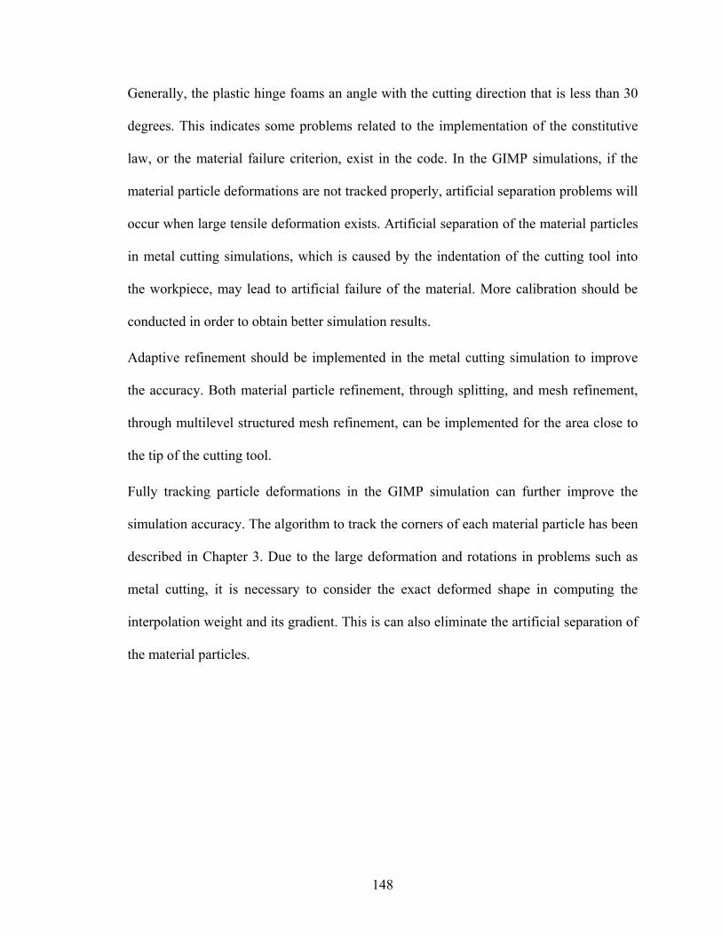
148
Generally, the plastic hinge foams an angle with the cutting direction that is less than 30
degrees. This indicates some problems related to the implementation of the constitutive
law, or the material failure criterion, exist in the code. In the GIMP simulations, if the
material particle deformations are not tracked properly, artificial separation problems will
occur when large tensile deformation exists. Artificial separation of the material particles
in metal cutting simulations, which is caused by the indentation of the cutting tool into
the workpiece, may lead to artificial failure of the material. More calibration should be
conducted in order to obtain better simulation results.
Adaptive refinement should be implemented in the metal cutting simulation to improve
the accuracy. Both material particle refinement, through splitting, and mesh refinement,
through multilevel structured mesh refinement, can be implemented for the area close to
the tip of the cutting tool.
Fully tracking particle deformations in the GIMP simulation can further improve the
simulation accuracy. The algorithm to track the corners of each material particle has been
described in Chapter 3. Due to the large deformation and rotations in problems such as
metal cutting, it is necessary to consider the exact deformed shape in computing the
interpolation weight and its gradient. This is can also eliminate the artificial separation of
the material particles.
149
Disclaimer on SAMRAI
The SAMRAI code was prepared as an account of work sponsored by an agency of the
United States Government. Neither the United States Government nor the University of
California nor any of their employees, makes any warranty, express or implied, or
assumes any legal liability or responsibility for the accuracy, completeness, or usefulness
of any information, apparatus, product, or process disclosed, or represents that its use
would not infringe privately owned rights. Reference herein to any specific commercial
product, process, or service by trade name, trademark, manufacturer, or otherwise, does
not necessarily constitute or imply its endorsement, recommendation, or favoring by the
United States Government or the University of California. The views and opinions of
authors expressed herein do not necessarily state or reflect those of the United States
Government or the University of California, and shall not be used for advertising or
product endorsement purposes.

150
References
ABAQUS Inc. (2005): ABAQUS Documentation, v6.5. Amodeo, R.J.; Ghoniem, N.M. (1990): Dislocation dynamics I. A proposed methodology for deformation micromechanics. Physical Review B, v41, pp. 6958-6966. Ashby, M.F.; Evans, A.G.; Fleck, N.A.; Gibson, L.J. (2000): Metal foams: A design guide, Butterworth-Heinemann, Boston, MA. Atluri, S.N.; Zhu, T. (1998): A new meshless local Petrov-Galerkin (MLPG) approach in computational mechanics. Computational Mechanics, v22, pp. 117-127. Atluri, S.N.; Zhu, T. (2000): New concepts in meshless methods. International Journal for Numerical Methods in Engineering, v47, n1, pp. 537–556. Atluri, S.N.; Zhu, T. (2000): The meshless local Petrov-Galerkin (MLPG) approach for solving problems in elasto-statics. Computational Mechanics, v25, pp. 169-179. Atluri, S.N.; Shen, S. (2002): The meshless local Petrov-Galerkin (MLPG) method: A simple and less-costly alternative to the finite element and boundary element methods. Computer Modeling in Engineering & Sciences, v3, n1, pp. 11-51. Bardenhagen, S.G.; Brydon, A.D.; Guilkey, J.E. (2005): Insight into the physics of foam densification via numerical simulation. J. Mech. Phys. Solids, v53, pp. 597-617. Bardenhagen, S.G. (2002): Energy conservation error in the material point method for solid mechanics. Journal of Computational Physics, v180, pp. 383-403. Bardenhagen, S.G.; Kober, E.M. (2004): The generalized interpolation material point method. Computer Modeling in Engineering & Sciences, v5, n6, pp. 477-496. Berger, M.J.; Oliger, J. (1984): Adaptive mesh refinement for hyperbolic partial differential equations. Journal of Computational Physics, v82, pp. 484-512. Bernstein, N.; Aziz, M.J.; Kaxiras, E. (2000): Atomistic simulations of solid-phase epitaxial growth in silicon. Physical Review B, v61, n10, pp. 6696-6700. Brydon, A.D.; Bardenhagen, S.G.; Miller, E.A.; Seidler, G.T. (2005): Simulaiton of the densification of real open-celled foam microstructures, J. Mech. Phys. Solids, v53, n12, pp. 2638-2660. Brothers, A.H.; Dunand, D.C. (2004): Syntactic bulk metallic glass foam. Applied Physics Letters, v84, n7, pp. 1108-1110. Brother, A.H.; Dunand, D.C. (2005): Ductile bulk metallic glass foams. Advanced Materials, v17, n4, pp. 484-486. Brother, A.H.; Dunand, D.C. (2006): Amorphous metal foams. Scripta Materialia, v54, pp. 513–520.

151
Brown, K.; Attaway, S.; Plimpton, S.; Hendrickson, B. (2000): Parallel strategies for crash and impact simulations. Computer Methods in Applied Mechanics and Engineering, v184, pp. 375-390.
Buehler, M.J.; Abraham, F.F.; Gao, H. (2003): Hyperelasticity governs dynamic fracture at a critical length scale. Nature, v426, pp. 141-146.
Buehler, M.J.; Gao H.; Huang, Y. (2004): Atomistic and continuum studies of stress and strain fields near a rapidly propagating crack in a harmonic lattice. Theor. Appl. Frac. Mech., v41, pp. 21-42.
Cai, W.; Koning, M.; Bulatov, V.; Yip, S. (2000): Minimizing boundary reflections in coupled-domain simulations. Physics Review Letter, v85, n15, pp. 3213-3216.
Conner, R.D.; Johnson, W.L.; Paton, N.E.; Nix, W.D. (2003): Shear bands and cracking of metallic glass plates in bending. Journal of Applied Physics, v94, n2, pp. 904-911.
Curtin, W.A.; Miller, R.E. (2003): Atomistic/continuum coupling in computational materials science. Modelling and Simulation in Materials Science and Engineering, v11, R33-R68.
Demetriou, M.D.; Hanan, J.D.; Veazey, C.; Michiel M.D.; Lenoir, N.; Ustundag, E.; Johnson, W.L. (2005): Mechanism of collapse of amorphous metallic foam, manuscript. Demetriou, M.D.; Hanan, J.D.; Veazey, C.; Michiel M.D.; Lenoir, N.; Ustundag, E.; Johnson, W.L. (2006): Cooperative yielding of amorphous metallic foam, manuscript. Fang, X.F.; Dahl, W. (1993): Investigation of the formation of dislocation cell structures and the strain hardening of metals by computer simulation. Materials Science and Engineering A, v164, pp. 300-305.
Gao, H.; Huang, Y.; Abraham, F.F. (2001): Continuum and atomistic studies of intersonic crack propagation. J. Mech. Phys. Solids, v49, pp. 2113-2132.
Gibson L.J.; Ashby, M.F. (1997): Cellular solids: structure and properties. 2nd ed. Cambridge University Press.
Gladwell, G.M.L. (1980): Contact Problems in the Classical Theory of Elasticity, SIJTHOFF & NOORDHOFF.
Groma, I.; Pawley, G.S. (1993): Role of the secondary slip system in a computer simulation model of the plastic behaviour of single crystals. Materials Science and Engineering A, v164, pp. 306-311.
Guilkey, J.E. (2005): Use of MPM in fully Lagrangian mode to eliminate cell crossing error. First MPM Workshop, March 13-14, 2005, Salt Lake City, Utah. Guilkey, J.E.; Weiss, J.A. (2003): Implicit time integration for the material point method: Quantitative and algorithmic comparisons with the finite element method. International Journal for Numerical Methods in Engineering, v57, pp. 1323-1338. Gulluoglu, A.N.; Hartley, C.S. (1993): Simulation of dislocation microstructures in two dimensions: II. Dynamic and relaxed structures. Modelling and Simulation in Materials Science and Engineering, v1, pp. 383-402.

152
Guo, Y.; Nairn, J. (2003): Calculation of J-integral and stress intensity factors using the material point method. Computer Modeling in Engineering & Sciences, v6, n3, pp. 295-308. Hanan, J.C.; Demetriou, M.D.; Veazey, C.; DeCarlo, F.; Thompson, S. (2005): Microtomotraphy of Amorphous Metal During Thermo-Plastic Foaming. Adv. X-Ray Anal., v49, in press. Hanan, J.C.; Johnson, W.L.; Peker, A. (2005): NASA NTR-41102. Hirth, J.P.; Lothe, J. (1982): Theory of Dislocations. John Wiley & Sons, 2nd ed. Hornung, R.D.; Kohn, S.R. (2002): Managing application complexity in the SAMRAI object-oriented framework. Concurrency and Computation: Practice and Experience, v14, pp. 347-368.
Horstemeyer, M.F.; Baskes, M.I. (2000): Strain tensors at the atomistic scale. Mat. Res. Soc. Symp. Proc., v578, pp. 15-20.
Horstemeyer, M.F.; Baskes, M.I.; Prantil, V.C.; Philliber, J.; Vonderheide, S. (2003): A multiscale analysis of fixed-end simple shear using molecular dynamics, crystal plasticity, and a macroscopic internal state variable theory. Modelling and Simulation in Materials Science and Engineering, v11, pp. 265-286l. Hufnagel, T.C. (2005): Metallic glass research at John Hopkins University, world wide web URL: http://www.jhu.edu/~matsci/people/faculty/hufnagel/background.html. Hsien, S.H. (1997): Evaluation of automatic domain partitioning algorithms for parallel finite element analysis. International Journal for Numerical Methods in Engineering, v40, pp. 1025-1051. Hu, W.; Chen, Z. (2003): A multi-mesh MPM for simulating the meshing process of spur gears. Computers & Structures, v81, pp. 1991-2002. Johnson, G.R.; Cook, W.H. (1983): A constitutive model and data for metals subjected to large strains, high strain rates and high temperatures. Proc. 7th International Symposium on Ballistics, pp. 541-547. Johnson, G.R.; Cook, W.H. (1985): Fracture characteristics of three metals subjected to various strains, strain rates, temperatures and pressures, Int. J. Engineering Fracture Mechanics, v21, pp. 31-48. Johnson, W.L; Samwer, K. (2005): A universal criterion for plastic yielding of metallic glasses with a (T/Tg)2/3 temperature dependence. Physics Review Letters, v95, n19, pp. 195501. Jones, R.M. (1999): Mechanics of Composite Materials, 2nd ed., Taylor & Francis, pp. 127. Kadar, Cs.; Maire, E.; Borbely, A.; Peix, G.; Lendvai, J.; Rajkovits, Zs (2004): X-Ray tomography and finite element simulation of the indentation behavior of metal foams. Materials Science and Engineering A, v387-389, pp. 321-325. Kalia, R.K.; Nakano, A.; Greenwell, D.L.; Vashishta, P. (1993): Parallel algorithms for molecular dynamics simulations on distributed memory MIMD machines. Supercomputer, v54, pp. 11-25. Katti, A.; Nilesh, S.; Samit, R.; Lu, H.; Fabrizio, E.F.; Dass, A.; Capadona, L.A.; Leventis, N. (2006): Chemical, physical, and mechanical characterization of isocyanate
153
cross-Linked amine-modified silica aerogels. Chemistry of Materials, v18, n2, pp. 285-296. Kannien, M.F. (1973): An augmented double cantilever beam model for studying crack propagation and arrest. Int. J. Fracture, v9, pp. 646-664. Kelchner, C.; Plimpton, S.; Hamilton, J. (1998): Dislocation nucleation and defect structure during surface indentation. Physical Review B, v58, n17, pp. 11085-11088.
Kohlhoff, S.; Gumbsch, P.; Fischmeister, H.F. (1991): Crack propagation in b.c.c. crystals studied with a combined finite-element and atomistic model. Phil. Mag. A, v64, n4, pp. 851-878.
Komanduri, R.; Lu, H.; Roy, S.; Wang, B.; Raff, L.M. (2004): Multiscale modeling and simulation for materials processing. Proceedings of the AFOSR Metallic Materials (2306 AX) Grantees Meeting, VA, USA. Kubin, L.P.; Canova, G. (1992): The modelling of dislocation patterns. Scripta Met., v27, pp. 957-962. Ma, J.; Lu, H.; Wang, B.; Roy, S.; Hornung, R.; Wissink, A.; Komanduri, R. (2005): Multiscale simulations using generalized interpolation material point (GIMP) method and SAMRAI parallel processing. Computer Modeling in Engineering & Sciences, v8, n2, pp. 135-152. Ma, J.; Lu, H.; Komanduri, R. (2006): Structured mesh refinement in generalized interpolation material point (GIMP) method for simulation of dynamic problems. Computer Modeling in Engineering & Sciences, (in press). Mackerle, J. (2003): FEM and BEM parallel processing: theory and applications-a bibliography. Engineering Computation, v20, n4, pp. 436-484.
Marc, G.; McMillan, W.G. (1985): The virial theorem. Adv. Chem. Phys., v58, pp. 209-361.
Meguid, S.A.; Heyerman, J.; Stranart, J.C. (2002): Finite element modeling of the axial collapse of foam-filled structures. J. Spacecraft and Rockets, v39, n6, pp. 828-832.
Meguid, S.A.; Stranart, J.C.; Heyerman, J. (2004): On the layered micromechanical three-dimensional finite element modeling of foam-filled columns. Finite Elements in Analysis and Design, v40, pp. 1035-1057.
Miller, R.E. (2000): A continuum plasticity model for the constitutive and indentation behaviour of foamed metals. International Journal of Mechanical Sciences, v42, pp. 729-754. Miller, R.E.; Shilkrot, L.E.; Curtin, W.A. (2004): A coupled atomistics and discrete dislocation plasticity simulation of nanoindentation into single crystal thin films. Acta Materialia, v52, n2, pp. 271-284. Oden, J.T.; Pires, E.B. (1983): Numerical analysis of certain contact problems in elasticity with non-classical friction laws. Computers & Structures, v16, n1-4, pp. 481-485. Pilkey, W.D. (1997): Peterson's Stress Concentration Factors, 2nd ed. John Wiley & Sons, New York.
154
Plimpton, S.J. (1995): Fast Parallel Algorithms for Short-Range Molecular Dynamics. Journal of Computational Physics, v117, pp. 1-19. Plimpton, S. (2005): Documentation for the LAMMPS Molecular Dynamics Simulator, Sandia National Laboratory.
Rafii-Tabar, H.; Hua, L.; Cross, L. (1998): A multi-scale atomistic-continuum modeling of crack propagation in a two-dimensional macroscopic plate. J. Phys.: Condens. Matter, v10, pp. 2375-2387.
Rybicki, E.F.; Kanninen, M.F. (1977): A finite element calculation of stress intensity factors by a modified crack closure integral. Engineering Fracture Mechanics, v9, pp. 931-938.
Rudd, R.E.; Broughton, J.Q. (1998): Coarse-grained molecular dynamics and the atomic limit of finite elements. Physical Review B, v58, n10, pp. R5893-5896.
Schroers, J.; Veazey, C.; Johnson, W.L. (2003): Amorphous metallic foam. Applied Physics Letters, v82, n3, pp. 370-372.
Shen, S.; Atluri, S.N. (2004a): Computational nano-mechanics and multi-scale simulation. Computers, Materials, & Continua, v1, n1, pp. 59-90. Shen, S.; Atluri, S.N. (2004b): Atomic-level stress calculation and continuum-molecular system equivalence. Computer Modeling in Engineering & Sciences, v6, n1, pp. 91-104. Shen, S.; Atluri, S.N. (2005): A tangent stiffness MLPG method for atom/continuum multiscale simulation. Computer Modeling in Engineering & Sciences, v7, n1, pp. 49-67.
Shilkrot, L.E.; Miller, R.E.; Curtin, W.A. (2002): Coupled atomistic and discrete dislocation plasticity. Physics Review Letter, v89, n2, 025501.
Shilkrot, L.E.; Miller, R.E.; Curtin, W.A. (2004): Multi-scale plasticity modeling: coupled atomistics and discrete dislocation mechanics. J. Mech. Phys. Solids, v52, pp.755-787.
Shiari, B.; Miller R.E.; Curtin, W.A. (2005): Coupled atomistic/discrete dislocation simulations of nanoindentation at finite temperature. J. Eng. Mater. Tech., v127, pp. 358-368.
Sulsky, D.; Schreyer, H.L. (1996): Axisymmetric foam of the material point method with applications to upsetting and Taylor impact problems. Computer Methods in Applied Mechanics and Engineering, v139, pp. 409-429. Sulsky, D.; Zhou, S.J.; Schreyer, H.L. (1995): Application of a particle-in-cell method to solid mechanics. Computer Physics Communications, v87, pp. 236-252. Tan, H.; Nairn, J.A. (2002): Hierarchical, adaptive, material point method for dynamic energy release rate calculations. Computer Methods in Applied Mechanics and Engineering, v191, pp. 2095-2109. Tewary, V.K.; Read, D.T. (2004): Integrated Green’s function molecular dynamics method for multiscale modeling of nanostructures: application to Au nanoisland in Cu. Computer Modeling in Engineering & Sciences, v6, n4, pp. 359-371. Third Wave Systems, Inc. (2006): AdvantEdge Documentation, v4.6.

155
van der Giessen, E.; Needleman, A. (1995): Discrete dislocation plasticity: a simple planar model. Modelling and Simulation in Materials Science and Engineering, v3, pp. 689-735. Wada, T.; Inoue, A. (2003): Fabrication, Thermal Stability and Mechanical Properties of Porous Bulk Glassy Pd-Cu-Ni-P Alloys. Materials Transactions, v44, n10, pp. 2228-2231. Wada, T.; Inoue, A.; Greer, A.L. (2005): Enhancement of room-temperature plasticity in a bulk metallic glass by finely dispersed porosity. Applied Physics Letters, v86, n25, pp. 251907. Wang, B.; Karuppiah, V.; Lu, H.; Roy, S.; Komanduri, R. (2005): Two-dimensional mixed mode crack simulation using the material point method. Mechanics of Advanced Materials and Structures, v12, pp. 471-484. Wicklein, M.; Thoma, K.; Vincenzini, P.; Lami (Eds.) A. (2004): Computational Modelling and Simulation of Materials III, Part A, Techna Group, Faenza, pp. 717–723. Wicklein, M.; Thoma, K. (2005): Numerical investigations of the elastic and plastic behavior of an open-cell aluminum foam. Materials Science and Engineering A, v397, pp. 391-399. Wissink, A.M.; Hysom, D.; Hornung, R.D. (2003): Enhancing scalability of parallel structured AMRA calculations. Proc. 17th ACM International Conference on Supercomputing (ICS03), San Francisco, CA, pp. 336-347. Zhong, Z.H. (1993): Finite Element Procedures for Contact-Impact Problems, Oxford University Press, New York.
Zhou, M.; McDowell, D.L. (2002): Equivalent continuum for dynamically deforming atomistic particle systems. Phil. Mag. A, v82, n13, pp. 2547-2574.
Zhu, H.X.; Mills, N.J.; Knott, J.F. (1997): Analysis of the high strain compression of open-cell foams. J. Mech. Phys. Solids, v45, n11/12, pp. 1875-1904. Zbib, H.M.; Diaz de la Rubia, T. (2002): A multiscale model of plasticity. International Journal of Plasticity, v18, n9, pp. 1133-1163. Zbib, H.M.; Rhee, M.; Hirth, J.P. (1998): On plastic deformation and the dynamics of 3D dislocations. International Journal of Mechanical Sciences, v40, pp. 113-127.
Zimmermann, J.A. (1999): Continuum and Atomistic Modeling of Dislocation Nucleation at Crystal Surface Ledges. Ph.D. dissertation, Stanford University.
Zimmermann, J.A.; Webb III, E.B.; Hoyt, J.J.; Jones, R.E.; Klein, P.A.; Bammann, D.J. (2004): Calculation of stress in atomistic simulation. Modelling and Simulation in Materials Science and Engineering, v12, S319-S332.

VITA
Jin Ma
Candidate for the Degree of
DOCTOR OF PHILOSOPHY
Thesis: MULTISCALE SIMULATION USING THE GENERALIZED INTERPOLATION MATEIRAL POINT METHOD, DISCRETE DISLOCATIONS AND MOLECULAR DYNAMICS
Major Field: Mechanical Engineering
Biographical:
Education: Received Associate Degree from Nantong Shipping College in Nantong, Jiangsu Province, P. R. China, in July, 1996; received Bachelor of Science degree in Mechanical Engineering and a minor in Computer Science from Wuhan University of Technology in Wuhan, Hubei Province, P. R. China, in June, 2000; received Master of Science degree with a major in Mechanical Engineering at Oklahoma State University, School of Mechanical and Aerospace Engineering in August, 2002; completed Doctor of Philosophy degree with a major in Mechanical Engineering at Oklahoma State University in May, 2006.
Experience: Employed by Oklahoma State University, School of Mechanical and
Aerospace Engineering as a graduate research and teaching assistant, from August, 2000 to July, 2002, and from August, 2003 to present.
Professional Membership: Certified National Programmer of China, Intermediate
Level, October, 1998.
2
Name: Jin Ma Date of Degree: May, 2006
Institution: Oklahoma State University Location: Stillwater, Oklahoma
Title of Study: MULTISCALE SIMULATION USING THE GENERALIZED INTERPOLATION MATERIAL POINT METHOD, DISCRETE DISLOCATIONS AND MOLECULAR DYNAMICS
Pages in Study: 155 Candidate for the Degree of Doctor of Philosophy
Major Field: Mechanical Engineering
Scope and Method of Study: A multiscale simulation scheme that spans the atomistic scale to the continuum has been developed for materials simulations in this study. At the continuum scale, the generalized interpolation material point (GIMP) method has been extended for parallel processing using the Structured Adaptive Mesh Refinement Application Infrastructure (SAMRAI). A contact algorithm in GIMP has been developed for the treatment of contact pair between a rigid indenter and a deformable workpiece. Two spatial refinement schemes for GIMP are presented for simulations with highly localized stress gradients at the continuum scale. A method for multiscale simulation bridging different scales, namely the continuum scale using GIMP, the mesoscale using discrete dislocations and the atomistic scale using the molecular dynamics (MD), is presented and validated in two dimensions.
Findings and Conclusions: Numerical simulations with multiple length scales from
nanometer to millimeter were conducted and validated on a 2D nanoindentation problem. Numerical simulations of several problems, such as tension, indentation, stress concentration and stress distribution near a crack (mode I crack problem) are presented to validate the refinement schemes at the continuum scale as well as the parallel processing algorithm. The capability of handling large deformation in GIMP is also demonstrated. A mode I crack propagation problem is simulated using the coupling algorithm. The stress field near the crack tip was validated by comparing results from coupled simulations with purely GIMP simulations of the same model. Coupled simulation results were also compared with purely MD simulations. A very good agreement was obtained. Other problems, such as dynamic friction problem at atomistic scale and the nanoindentation problem, are also simulated using the multiscale simulation algorithm.
Advisor’s Approval: Hongbing Lu