Moments for L-functions for GLr GLr 1

Moments for L-functions for GLr �GLr−1

A. Diaconu, P. Garrett, D. Goldfeld [email protected] http://www.math.umn.edu/ garrett/

1. The moment expansion2. Spectral expansion: reduction to GL2

3. Spectral expansion for GL2

4. Continuation and holomorphy at s′ = 0 for GL2

5. Spectral expansion for GLr6. Continuation and holomorphy at s′ = 0 for GLr7. Appendix: half-degenerate Eisenstein series8. Appendix: Eisenstein series for GL2

9. Appendix: residues of degenerate Eisenstein series for Pn−1,1

10. Appendix: degenerate Eisenstein series for P r−2,1,1

We exhibit elementary kernels Pe which produce sums of integral moments for cuspforms f on GLr by

∫ZAGLr(k)\GLr(A)

Pe · |f |2 =∑

F on GLr−1

∫Re(s)= 1

2

|L(s, f ⊗ F )|2

〈F, F 〉M(s) ds + (continuous part)

over number fields k, with certain weights M(s). Here F runs over an orthogonal basis for cuspformson GLr−1. There are further continuous-spectrum terms analogous to the discrete-spectrum sum overcuspforms. The kernel (Poincare series) Pe admits a spectral decomposition, surprisingly consisting of onlythree parts: a leading term, a sum arising from cuspforms on GL2, and a continuous part from GL2. Thatis, no cuspforms on GL` with 2 < ` ≤ r contribute. This spectral decomposition makes possible themeromorphic continuation of Pe in auxiliary parameters.

Moments of level-one holomorphic elliptic modular forms were treated in [Good 1983] and [Good 1986], thelatter using an idea that is a precursor of part of the present approach. Level-one waveforms overQ appear in[Diaconu-Goldfeld 2006a], over Q(i) in [Diaconu-Goldfeld 2006b]. Arbitrary level, groundfield, and ∞-typefor GL2 are in [Diaconu-Garrett 2006] and [Diaconu-Garrett 2008].

We do have in mind application not only to cuspforms, but also to truncated Eisenstein series (with cuspidaldata) or wave packets of Eisenstein series, giving a non-trivial application of harmonic analysis on largergroups GLr to L-functions attached to smaller groups, for example, on GL1, giving high integral momentsof ζk(s).

For context, we review the [Diaconu-Goldfeld 2006a] treatment of spherical waveforms f for GL2(Q). Inthat case, the sum of moments is a single term

∫ZAGL2(Q)\GL2(A)

Pe(g) |f(g)|2 dg =1

2πi

∫Re(s)= 1

2

L(s′ + s, f) · L(s, f) · Γ(s, s′, s′′, f∞) ds

where Γ(s, s′, s′′, f∞) is a ratios of products of gammas, with arguments depending upon the archimedeandata attached to f . Here the Poincare series Pe(g) = Pe(g, s′, s′′) has a spectral expansion

Pe(s′, s′′) =π

1−s′′2 Γ( s

′′−12 )

π−s′′2 Γ( s′′2 )

· E1+s′ + 12

∑F on GL2

L( 12 + s′, F )〈F, F 〉

· G( 12 − itF , s

′, s′′) · F

+1

4πi

∫Re(s)= 1

2

ζ(s′ + s) ζ(s′ + 1− s)ξ(2− 2s)

G(1− s, s′, s′′) · Es ds (for Re(s′)� 12 , Re(s′′)� 0)

1

Diaconu-Garrett-Goldfeld: Moments for L-functions for GLr ×GLr−1

where ξ(s) = π−s/2Γ(s/2)ζ(s), where G is essentially a product of gamma function values [1]

G(s, s′, s′′) = π−(s′+ s′′2 ) Γ( s

′+1−s2 ) Γ( s

′+s2 ) Γ( s

′−s+s′′2 ) Γ( s

′+s−1+s′′

2 )Γ(s′ + s′′

2 )

and F is summed over (an orthogonal basis for) spherical (at finite primes) cuspforms on GL2 with Laplacianeigenvalues 1

4 + t2F , and Es is the usual spherical Eisenstein series

Es

(y 00 1

)= |y|s +

ξ(2− 2s)ξ(2s)

|y|1−s + . . .

It is not obvious, but the continuous part (the integral of Eisenstein series) cancels the pole at s′ = 1 of theleading term, and when evaluated at s′ = 0 is [2]

Pe(g, 0, s′′) = (holomorphic at s′=0) +12

∑F on GL2

L( 12 , F )〈F, F 〉

· G( 12 − itF , 0, s

′′) · F

+1

4πi

∫Re(s)= 1

2

ζ(s) ζ(1− s)ξ(2− 2s)

G(1− s, 0, s′′) · Es ds

In this spectral expansion, the coefficient in front of a cuspform F includes G evaluated at s′ = 0 ands = 1

2 ± itF , namely

G( 12 − itF , 0, s

′′) = π−s′′2

Γ(12−itF

2 ) Γ(12 +itF

2 ) Γ(s′′− 1

2−itF2 ) Γ(

s′′− 12 +itF

2 )Γ( s′′2 )

The gamma function has poles at 0,−1,−2, . . ., so this coefficient has poles at s′′ = 12 ± itF , − 3

2 ± itF , . . ..Over Q, among spherical cuspforms (or for any fixed level) these values have no accumulation point. [3] Thecontinuous part of the spectral side at s′ = 0 is

14πi

∫Re(s)= 1

2

ξ(s) ξ(1− s)ξ(2− 2s)

Γ( s′′−s2 ) Γ( s

′′−1+s2 )

Γ( s′′2 )· Es ds

with gamma factors grouped with corresponding zeta functions, to form the completed L-functions ξ.Thus, the evident pole of the leading term at s′′ = 1 can be exploited, using the obvious continuationto Re(s′′) > 1/2.

Further, a subtle contour-shifting argument[4] shows that the continuous part of this spectral decompositionhas a meromorphic continuation to C with poles at ρ/2 for zeros ρ of ζ, in addition to the obvious polesfrom the gamma functions.

[1] This from [Diaconu-Goldfeld 2006a], the result of a direct computation with the simplest useful choice of

archimedean data in the Poincare series.

[2] This evaluation of the meromorphic continuation, from [Diaconu-Goldfeld 2006a], is not trivial. Note that the

leading term (after continuation) is reminiscent of the Kronecker limit formula. See [Asai 1977].

[3] The discreteness of the parameters tF as F ranges over cuspforms of a fixed level follows from the compactness

of test-function operators on cuspforms, from [Gelfand-PS 1963]. In particular, at this point we do not need any sort

of Weyl’s law, and, thus, do not need trace formula computations yet.

[4] See [Diaconu-Goldfeld 2006a]. A contour shifting argument is also necessary to meromorphically continue the

continuous part of the spectral decomposition to s′ = 0 in the first place.

2


Already for GL2, over general groundfields k, infinitely many Hecke characters enter [5] both the spectraldecomposition of the Poincare series and the moment expression. This naturally complicates isolation ofliteral moments, and complicates analysis of poles via the spectral expansion. Suppressing constants, themoment expansion is a sum of twists by χ’s∫

ZAGL2(k)\GL2(A)

Pe · |f |2 =∑χ

∫Re(s)= 1

2

L(s′ + s, f ⊗ χ) · L(1− s, f ⊗ χ) ·Mχ(s) ds

And, suppressing constants, the spectral expansion is

Pe = (∞− part) · E1+s′ +∑

F on GL2

(∞− part) ·L( 1

2 + s′, F )〈F, F 〉

· F

+∑χ

∫Re(s)= 1

2

L(s′ + s, χ)L(s′ + 1− s, χ)L(2− 2s, χ2)

Gχ(s) · Es,χ ds

In the simplest case beyond GL2, take f a spherical cuspform [6] on GL3 over [7] Q. We construct a weightfunction Γ(s, s′, s′′, f∞, F∞) depending upon complex parameters s, s′, and s′′, and upon the archimedeandata for both f and cuspforms F on GL2, such that Γ(s, s′, s′′, f∞, F∞) has explicit asymptotic behavior,and such that the moment expansion is∫

ZAGL3(Q)\GL3(A)

Pe(s′, s′′) · |f |2 dg =∑

F on GL2

12πi

∫Re(s)= 1

2

|L(s, f ⊗ F )|2

〈F, F 〉· Γ(s, 0, s′′, f∞, F∞) ds

+1

4πi1

2πi

∑k∈Z

∫Re(s1)= 1

2

∫Re(s2)= 1

2

|L(s1, f ⊗ E(k)1−s2)|2

|ξ(1− 2it2)|2· Γ(s1, 0, s′′, f∞, E

(k)1−s2,∞) ds1 ds2

where F runs over (an orthogonal basis for) all level-one cuspforms on GL2, with no restriction on theright K∞-type, and E

(k)s is the usual level-one Eisenstein series of K∞-type k. Here and throughout, for

Re(s) = 1/2, write 1 − s in place of s, to maintain holomorphy in complex-conjugated parameters. In thisvein, over Q, it is reasonable to put

L(s1, f ⊗ E(k)

s2 ) = L(s1, f ⊗ E(k)1−s2) =

L(s1 + 12 − s2, f) · L(s1 − 1

2 + s2, f)ζ(2− 2s2)

(finite-prime parts only)

since the natural normalization of the Eisenstein series E(k)s2 on GL2 contributes the denominator ζ(2−2s2).

Meromorphic continuation in s′ and evaluation at s′ = 0 gives the desired specialization of the momentexpansion. There is also a meromorphic continuation in the parameter s′′ in the archimedean data.

More generally, for a cuspform f on GLr with r ≥ 3, whether over Q or over a numberfield, the momentexpansion includes an infinite sum [8] of |L(s, f ⊗ F )|2/〈F, F 〉 over an orthogonal basis for cuspforms F

[5] See [Sarnak 1985], [Diaconu-Goldfeld 2006b] for Q(i), and [Diaconu-Garrett 2006] for number fields.

[6] For our purposes, a cuspform generates an irreducible unitary representation of the adele group, so has a central

character, and the representation factors over primes. This factorization follows from the admissibility of irreducible

unitaries of reductive groups over archimedean and non-archimedean local fields (the former due to Harish-Chandra

in the 1950s, the latter reduced to the supercuspidal case by Harish-Chandra, and completed by J. Bernstein in 1972).

[7] The assumption of groundfield Q achieves the minor simplification that for GL2(Q) there is a single (family of)

Eisenstein series participating in the spectral decomposition.

[8] In fact, it is non-trivial to prove (after Selberg) that there are infinitely-many spherical waveforms for SL2(Z).

3


on GLr−1, as well as integrals of products of L-functions L(s, f ⊗ F ) for F ranging over cuspforms onGLr1 × . . . × GLr` for all partitions (r1, . . . , r`) of r. Correspondingly, the natural normalization of thecuspidal-data Eisenstein series gives products of convolution L-functions L(∗, Fi ⊗ Fj) in the denominatorsof these terms, as well as factors 〈Fi, Fi〉1/2 · 〈Fj , Fj〉1/2. [9]

Generally, the spectral expansion for GLr is an induced-up version of that for GL2. Suppressing constants,using groundfield Q to skirt Hecke characters,

Pe = (∞− part) · Er−1,1s′+1 +

∑F on GL2

(∞− part) ·L( rs

′+r−22 + 1

2 , F )〈F, F 〉

· Er−2,2s′+1

2 ,F

+∫

Re(s)= 12

(∞− part) ·ζ( rs

′+r−22 + 1

2 − s) · ζ( rs′+r−2

2 + 12 + s)

ζ(2− 2s)· Er−2,1,1

s′+1, s− s′+12 ,−s− s′+1

2

ds

where the Eisenstein series are normalized naively. The continuous part has a pole that cancels the obviouspole of the leading term at s′ = 0.

Again over Q, the most-continuous part of the moment expansion for GLn is of the form∫Re(s)= 1

2

∫t∈Λ

|L(s, f ⊗ Emin12 +it

)|2Mt(s) ds dt =∫ ∫

Λ

∣∣∣∣ Π1≤`≤n−1 L(s+ it`, f)Π1≤j<`<n ζ(1− itj + it`)

∣∣∣∣2 Mt(s) ds dt

whereΛ = {t ∈ Rn−1 : t1 + . . .+ tn−1 = 0}

and where M is a weight function depending upon f and F . More generally, let n − 1 = m · b. For F onGLm, let

F∆ = F ⊗ . . .⊗ Fon GLm × . . .×GLm. Inside the moment expansion we have (recall Langlands-Shahidi)∫

Re(s)= 12

∫Λ

|L(s, f ⊗ EF∆, 12 +it)|2MF,t(s) ds dt =

∫ ∫ ∣∣∣∣ Π1≤`≤b L(s+ it`, f ⊗ F )Π1≤j<`≤b L(1− itj + it`, F ⊗ F∨)

∣∣∣∣2M dsdt

If we replace the cuspform f on GLn(Q) by a (truncated) minimal-parabolic Eisenstein series Eα withα ∈ Cn−1, the most-continuous part of the moment expansion contains a term∫ ∫

Λ

∣∣∣∣Π1≤µ≤n, 1≤`≤n−1 ζ(αµ + s+ it`)Π1≤j<`<n |ζ(1− itj + it`)

∣∣∣∣2 ds dtTaking α = 0 ∈ Cn−1 gives ∫ ∫

Λ

∣∣∣∣ Π1≤`≤n−1 ζ(s+ it`)n

Π1≤j<`<n ζ(1− itj + it`)

∣∣∣∣2 M dsdt

For example, for GL3, where Λ = {(t,−t)} ≈ R,∫ ∫R

∣∣∣∣ζ(s+ it)3 · ζ(s− it)3

ζ(1− 2it)

∣∣∣∣2 M dsdt

and for GL4 ∫(s)

∫Λ

∣∣∣∣ ζ(s+ it1)4 · ζ(s+ it2)4 · ζ(s+ it3)4

ζ(1−it1+it2) ζ(1−it1+it3) ζ(1−it2+it3)

∣∣∣∣2M dsdt

[9] The identification of these denominators in the natural normalization of the Eisenstein series is part of the

refinement in [Shahidi 1978] and [Shahidi 1983] of [Langlands 1976]’s treatment of L-functions arising in constant

terms of these Eisenstein series. Here we need to keep track of constants, due to the average over F .

4


1. The moment expansion

Let G = GLr over a number field k. Let P be the standard maximal proper parabolic

P = P r−1,1 = {(

(r − 1)-by-(r − 1) ∗0 1-by-1

)}

Let

U = {(

1r−1 ∗0 1

)} H = {

((r − 1)-by-(r − 1) 0

0 1

)}

andN = {upper triangular unipotent elements in H}

= (unipotent radical of standard minimal parabolic in H)

Let Z be the center of G. Let Kv be the standard maximal compact in the kv-valued points Gv of G. Thus,for v <∞, Kv = GLr(ov). For v ≈ R, take Kv = Or(R). For v ≈ C take Kv = U(r).

The standard choice of non-degenerate character on NkUk\NAUA is

ψ(n · u) = ψ0(n12 + n23 + . . .+ nr−2,r−1) · ψ0(ur−1,r)

where ψ0 is a fixed non-trivial character on A/k. A cuspform [10] f has a Fourier expansion [12] along NU

f(g) =∑

ξ∈Nk\Hk

Wf (ξg) where Wf (g) =∫NkUk\NAUA

ψ(nu) f(nug) dn du

The (Whittaker) function Wf (g) factors over primes. [13]

[1.1] Poincare series For s′ ∈ C, letϕ =

⊗v

ϕv

where for v finite

ϕv(g) =

∣∣(detA)/dr−1

∣∣s′v

(for g = mk with m =(A 00 d

)in ZvHv and k ∈ Kv)

0 (otherwise)

[10] A cuspform f satisfies the Gelfand-Fomin-Graev condition [11] RNk\NA f(ng) dn = 0 for all unipotent radicals

N of (proper, rational) parabolics, generates an irreducible representation locally everywhere (hence, has a central

character ω), and is in L2(ZAGk\GA, ω).

[12] Fourier-Whittaker expansions for GL(n) with n > 2 are due to [Shalika 1974] and [Piatetski-Shapiro 1975],

independently.

[13] Uniqueness of Whittaker models, by [Shalika 1974] at archimedean places, [Gelfand-Kazhdan 1975] at non-

archimedean, implies the factorization over primes. The local factors are ambiguous up to constants, naturally.

For cuspforms f at primes v where f is spherical, the spherical Whittaker function W ◦v with the same local data as

f , normalized by W ◦v (1) = 1, is the standard choice. However, even at good primes, for natural normalization in

construction of Eisenstein series presents us most naturally with a local Whittaker function which is an image under

the intertwining operator from principal series to the Whittaker model. This contributes an extra factor which is

a product of L-functions, as studied at length in [Langlands 1971], [Shahidi 1978], [Shahidi 1983], and elsehwere.

Luckily, our subsequent convolution L-functions will lack archimedean factors, so avoid the most acute concern about

choices of data at archimedean places, thus skirting issues addressed in [Jacquet-Shalika 1990], [Cogdell-PS 2003].

5


and for v archimedean require right Kv-invariance and left equivariance

ϕv(mg) =∣∣∣∣detAdr−1

∣∣∣∣s′v

· ϕv(g) (for g ∈ Gv, for m =(A 00 d

)∈ ZvHv)

Thus, for v|∞, the further data determining ϕv consists of its values on Uv. The simplest useful choice is[14]

ϕv

(1r−1 x

0 1

)= (1 + |x1|2 + . . .+ |xr−1|2)−s

′′/2 (where x =

x1...

xr−1

, and s′′ ∈ C)

and where the norm |x1|2 + . . . + |xr−1|2 is normalized to be invariant under Kv. [15] Thus, ϕ is leftZAHk-invariant. We attach to ϕ a Poincare series

Pe(g) =∑

γ∈ZkHk\Gk

ϕ(γg)

[1.2] Two obvious unwindings Integrate the norm-squared |f |2 of a cuspform f against Pe. The typicalfirst unwinding is ∫

ZAGk\GAPe(g) |f(g)|2 dg =

∫ZAHk\GA

ϕ(g) |f(g)|2 dg

Next, express f in its Fourier-Whittaker expansion, and unwind further:∫ZAHk\GA

ϕ(g)∑

ξ∈Nk\Hk

Wf (ξg) f(g) dg =∫ZANk\GA

ϕ(g)Wf (g) f(g) dg

[1.3] Iwasawa decomposition, simplification of integral Suppose for simplicity that f is right KA-invariant, so we can use an Iwasawa decomposition G = (HZ)UK (everywhere locally) to rewrite the wholeintegral as ∫

Nk\HA×UAϕ(hu)Wf (hu) f(hu) dh du

[1.4] Spectral decomposition on GLr−1 Use a spectral decomposition [16] for F ∈ L2(Hk\HA),inexplicitly

F =∫

(η)

〈F, η〉 · η dη

[14] Over Q and Q(i), in effect this is the choice of archimedean data in [Good 1983], [Diaconu-Goldfeld 2006a],

[Diaconu-Goldfeld 2006b].

[15] Thus, for this purpose, to be Kv-invariant at real places v, we use the standard norm. At complex places we also

use the standard norm, not the norm compatible with the product formula. That is, for this purpose, for v ≈ C the

norm is not |z|v = z · z, but is |z| =√z · z.

[16] Let H1 = {h ∈ HA : | deth| = 1}. Then Hk\HA = Hk\H1 × (0,+∞) is the relevant decomposition. The

most obvious continuous part coming from (0,+∞) will eventually give integrals over vertical lines. Still L2(Hk\H1)

has both continuous and discrete parts in its decomposition. Since some of the necessary functions η for such a

spectral decomposition are not literally in L2 (both Eisenstein series and ordinary exponentials in Fourier transforms

and Fourier inversion), the inner integral is not at all symmetric. Further, that integral, (as well as the outer)

only make literal sense for F in a suitable (dense) subspace (e.g., pseudo-Eisenstein series and Schwartz functions

in the corresponding circumstances), and the mappings indicated must be defined by isometric extension. See

[Langlands 1976] and [Moeglin-Waldspurger 1995].

6


where each η generates an irreducible representation of HA.

[1.5] Expand f(hu) Since f is left Hk-invariant, it decomposes along Hk\HA as

f(hu) =∫

(η)

η(h)∫Hk\HA

η(m) f(mu) dmdη

Unwind the Fourier-Whittaker expansion of f

f(hu) =∫

(η)

η(h)∫Hk\HA

η(m)∑

ξ∈Nk\Hk

W f (ξmu) dmdη

=∫

(η)

η(h)∫Nk\HA

η(m)W f (mu) dmdη

Then the whole integral is ∫ZAGk\GA

Pe(g) |f(g)|2 dg

=∫

(η)

∫Nk\HA×UA

ϕ(hu) η(h)Wf (hu)∫Nk\HA

W f (mu) η(m) dmdhdu dη

[1.6] Decoupling at finite primes The part of the integrand that depends upon u ∈ U is∫UA

ϕ(hu)Wf (hu)W f (mu) du = ϕ(h)Wf (h)W f (m) ·∫UA

ϕ(u)ψ(huh−1)ψ(mum−1) du

The latter integrand visibly factors over primes.

[1.6.1] Lemma: Let v be a finite prime. For h,m ∈ Hv such that Wf,v(h) 6= 0 and W f,v(m) 6= 0,∫Uv

ϕv(h)ψv(huh−1)ψv(mum−1) du =

∫Uv∩Kv

1 du

Proof: At a finite place v, ϕv(u) 6= 0 if and only if u ∈ Uv ∩Kv, and for such u

ψv(huh−1) ·Wf,v(h) = Wf,v(huh−1 · h) = Wf,v(hu) = Wf,v(h) · 1

by the right Kv-invariance. Thus, for Wf,v(h) 6= 0, ψv(huh−1) = 1, and similarly for ψv(mum−1). Thus,the finite-prime part of the integral over Uv is just the integral of 1 over Uv ∩Kv, as indicated. ///

[1.7] Archimedean kernel The archimedean part of the integral does not necessarily decouple. Thus,with subscripts ∞ denoting the infinite-adele part of various objects, for h,m ∈ H∞, define

K(h,m) =∫U∞

ϕ∞(u)ψ∞(huh−1)ψ∞(mum−1) du

The whole integral is∫ZAGk\GA

Pe(g) |f(g)|2 dg =∫

(η)

∫Nk\HA

∫Nk\HA

K(h,m)ϕ(h)(Wf (h) η(h)

)(W f (m) η(m)

)dmdhdη

7


[1.8] Fourier expansion of η Normalize the volume of Nk\NA to 1. Thus, for a left Nk-invariant functionF on HA ∫

Nk\HAF (h) dh =

∫NA\HA

∫Nk\NA

F (nh) dn dh

Using the left NA-equivariance of W by ψ, and the left NA-invariance of ϕ,∫Nk\NA

ϕ(nh) η(nh)Wf (nh) dn = ϕ(h)Wf (h)∫Nk\NA

ψ(n) η(nh) dn = ϕ(h)Wf (h)Wη(h)

whereWη(h) =

∫Nk\NA

ψ(n) η(nh) dn

(The integral is not against ψ(n), but ψ(n).) That is, the integral over Nk\HA is equal to an integral against(up to an alteration of the character) the Whittaker function Wη of η, which factors [17] over primes. Thewhole integral is∫

ZAGk\GAPe(g) |f(g)|2 dg =

∫(η)

∫NA\HA

∫NA\HAK(h,m)ϕ(h)

(Wf (h)Wη(h)

)(W f (m)W η(m)

)dmdhdη

And the ηth part is a product of two Euler products. It is evident that for f right Kfin-invariant onlyright (Kfin ∩Hfin)-invariant η’s will appear, due to the decoupling. However, at archimedean places v rightKv-invariance of f does not allows us to restrict our attention to right (Kv ∩Hv)-invariant η.

[1.9] Appearance of the parameter s In fact, as usual,

Hk\HA ≈ GLr−1(k)\GLr−1(A) ≈ R+ ×Hk\H1

where R+ is positive real numbers, and

H1 = {(a 00 1

): a ∈ GLr−1(A), |det a| = 1}

The quotient Hk\H1 has finite volume. Thus, the spectral decomposition uses functions

η

(a 00 1

)= |det a|s · F (a) with F ∈ L2(Hk\H1), s ∈ iR

The real part of the parameter s will necessarily be shifted in the subsequent discussion. Thus, the functionsη above are of the form |det |s ⊗ F , and the Whittaker function Wη of η = |det |s ⊗ F is

Wη

(a

1

)= |det a|s ·WF (a)

where WF is the Whittaker function of F , normalized here by

WF (g) =∫Nk\NA

ψ(n)F (ng) dn

[17] When η is either a cuspform (in a strong sense) or is an Eisenstein series attached to suitable (e.g., cuspidal,

in a strong sense) data, this Whittaker function Wη factors over primes. The usual normalization for the spherical

Whittaker function W ◦v at finite places v is W ◦v (1) = 1. This is the normalization we take for cuspforms, but this

is incompatible with a standard normalization of Eisenstein series E(g) =Pγ ϕ(γg) by requiring ϕ(1) = 1. This

produces a normalizing denominator which (as in simple cases of Langlands-Shahidi) is a product of convolution

L-functions.

8


where N is the unipotent radical of the standard minimal parabolic in GLr−1.

[1.10] Non-archimedean local factors

In terms of s and F , the non-archimedean local factors are [18]∫Nv\Hv

|det a|s+s′Wf,v

(a

1

)WF,v(a) da =

Lv(s+ s′ + 12 , f ⊗ F )

〈F, F 〉1/2(for Re(s+ s′)� 0)

The second Euler product is the complex conjugate of this, but lacking the shift by s′, namely, the complexconjugate of∫Nv\Hv

|det a′|sWf,v

(a′

1

)WF,v(a′) da′ =

Lv(s+ 12 , f ⊗ F )

〈F, F 〉1/2(for Re(s+ s′)� 0 and Re(s)� 0)

When η = |det |s ⊗ F is not cuspidal, but, instead, is an Eisenstein series with cuspidal data, it still doesgenerate an irreducible representation of GA. At a place v where η generates a spherical representation, theEuler product expansion of degree r · (r − 1) falls apart into smaller factors, and has a denominator arisingfrom the (natural) normalization of the cuspidal-data Eisenstein series entering. Discussion of these termsand their normalizations is postponed.

[1.11] Replace s by 1− s on Re(s) = 1/2

The global integrals for the L-functions L(s′+s+ 12 , f⊗F ) and L(s+ 1

2 , f⊗F ) only converge for Re(s′+s)� 0and Re(s) � 0, so we will need to meromorphically continue. To this end, it is most convenient for thewhole integral to be holomorphic in s, rather than having both s and s appear.

To these ends, first absorb the 1/2 into s by replacing s by s+ 12 , so we have

L(s′ + s, f ⊗ F ) · L(s, f ⊗ F )

and want to eventually move to the line Re(s) = 1/2. To avoid the anti-holomorphy in the second factor,since s = 1− s on the line Re(s) = 1/2, we can rewrite this as

L(s′ + s, f ⊗ F ) · L(1− s, f ⊗ F ) (for Re(1− s)� 0 and Re(s′ + s)� 0)

[1.12] The vertical integral(s) Keep in mind that we have absorbed a 1/2 into s, and have replaced sby 1− s. The archimedean part of the whole integral is the function Γϕ∞(s, s′, f, F ) defined by

Γϕ∞(s, s′, f, F ) =∫N∞\H∞

∫N∞\H∞

K(h,m) |det a|s′+s− 1

2 |det a′| 12−s(Wf,∞

(a

1

)WF,∞(a)

)×

(W f,∞

(a′

1

)WF,∞(a′)

)da da′ (with h =

(a

1

)and m =

(a′

1

))

[18] The L-functions L(s, f ⊗ F ) attached to cuspforms f and F by these zeta integrals are Euler products with local

factor equal to that of the L-functions L(s, πf ×πF ) attached to the corresponding (irreducible cuspidal automorphic)

representations at all finite primes at which f and F are spherical. At other finite places the local factors of L(s, f⊗F )

may be polynomial (in q−sv and qsv) multiples of the corresponding local factor of L(s, πf × πF ). At archimedean

places, Lv(s, f ⊗ F )/Lv(s, πf × πF ) is entire, etc. Last, but not least, there are global constant factors sometimes

denoted ρf (1) which for newforms f for GL(2) are the ratios of the first Fourier coefficient of f to the Petersson norm

squared of f . See [Hoffstein-Lockhart 1994], [Bernstein-Reznikoff 1999], and [Sarnak 1985], [Sarnak 1992]. Here the

latter global normalizing constant is accommodated by a division by 〈F, F 〉1/2, to make F/〈F, F 〉1/2 run through an

orthonormal basis when F runs through an orthogonal basis.

9


since ϕ∞(h) = |det a|s′ . Note that this depends only upon the archimedean data attached to f and F .Thus, so far, the whole is ∫

ZAGk\GAPe(g) |f(g)|2 dg

=∑

F on GL(r−1)

∫Re(s)= 1

2

Γϕ∞(s, s′, f, F )L(s′ + s, f ⊗ F )L(1− s, f ⊗ F )

〈F, F 〉dt

+ (continuous part) (with Re(s′)� 0)

Again, we want to meromorphically continue to s′ = 0.

[1.12.1] Remark: With or without detailed knowledge of the residual part of L2 (meaning that consistingof square-integrable iterated residues of cuspidal-data Eisenstein series), automorphic forms in the residualspectrum not admitting Whittaker models do not enter in this expansion.

2. Spectral expansion: reduction to GL2

The Poincare series admits a spectral expansion in terms of Eisenstein series, cuspforms, and L-functions,preparing for its meromorphic continuation. This section reduces the general spectral expansion to the caser = 2.

[2.1] Poisson summation Form the Poincare series in two stages to allow application of Poissonsummation, namely

Pe(g) =∑

ZkHk\Gk

ϕ(γg) =∑

ZkHkUk\Gk

∑β∈Uk

ϕ(βγg) =∑

ZkHkUk\Gk

∑ψ∈(Uk\UA)bϕγg(ψ)

where

ϕg(ψ) =∫UA

ψ(u)ϕ(ug) du (for g ∈ GA)

[2.2] The leading term The inner summand for ψ = 1 gives a vector from which an extremely degenerateEisenstein series [19] for the (r − 1, 1) parabolic P r−1,1 = ZHU is formed by the outer sum. That is,

g →∫UA

ϕ(ug) du

is left equivariant by a character on P r−1,1A , and is left invariant by P r−1,1

k , namely,∫UA

ϕ(upg) du =∫UA

ϕ(p · p−1up · g) du = δP r−1,1(m) ·∫UA

ϕ(m · u · g) du

=∣∣∣∣detAdr−1

∣∣∣∣s′+1 ∫UA

ϕ(ug) du (where p =(A ∗0 d

), A ∈ GLr−1, d ∈ GL1)

[19] These degenerate (spherical) Eisenstein series Er−1,1s are readily understood via Poisson summation, imitating

Riemann et alia. There is a simple pole at s = 1, with constant residue, and no other poles in Re(s) ≥ 1/r. That

first pole will be cancelled (when s′ goes to 0) by the continuous part of the spectral decomposition.

10


The normalization [20] is explicated by setting g = 1:∫UA

ϕ(u) du =∫U∞

ϕ∞ ·∫Ufin

ϕfin =∫U∞

ϕ∞ ·meas (Ufin ∩Kfin) =∫U∞

ϕ∞

A natural normalization would have been that this value be 1, so the Eisenstein series here implicitly includesthe archimedean integral and finite-prime measure constant as factors:∫

U∞

ϕ∞ · Er−1,1s′+1 (g) =

∑γ∈P r−1,1

k \Gk

(∫UA

ϕ(uγg) du)

As advance warning: the pole at s′ = 0 of this leading term will be cancelled by a contribution from thecontinuous part of the spectral decomposition, below.

[2.3] Main terms: appearance of Q from GL2 The group Hk is transitive on non-trivial characterson Uk\UA. As usual, for fixed non-trivial character ψ0 on k\A, let

ψξ(u) = ψ0(ξ · ur−1,r) (for ξ ∈ k×)

The spectral expansion of Pe with the obvious leading term removed, is

∑γ∈P r−1,1

k \Gk

∑α∈P r−2,1

k \Hk

∑ξ∈k×

ϕαγg(ψξ)

where P r−2,1 is the parabolic subgroup of H ≈ GLr−1. Let

U ′ = {

1r−2 ∗1

1

} U ′′ = {

1r−2

1 ∗1

}Let

Θ = {

1r−2

∗ ∗∗ ∗

}Then the expansion of the Poincare series with leading term removed is

∑γ∈P r−2,1,1

k \Gk

∑ξ∈k×

∫U ′′A

ψξ(u′′)

∫U ′A

ϕ(u′u′′γg) du′ du′′

=∑

γ∈P r−2,2k \Gk

∑α∈P 1,1\Θk

∑ξ∈k×

∫U ′′A

ψξ(u′′)

∫U ′A

ϕ(u′u′′αγg) du′ du′′

Letting

ϕ(g) =∫U ′A

ϕ(u′g) du′

[20] Recall an integration-theory trick. Given a unimodular topological groupG, use a topological group decomposition

G = PK with K compact open as follows. To integrate a right K-invariant function f on G, with the total mass of

K normalized to 1, we haveRG f =

RP f with a left Haar measure on P normalized so that the measure (in P ) of

K ∩ P is 1.

11


the expansion becomes ∑γ∈P r−2,2

k \Gk

∑α∈P 1,1\Θk

∑ξ∈k×

∫U ′′A

ψξ(u′′) ϕ(u′′αγg) du′′

We claim the equivariance

ϕ(pg) = |detA|s′+1 · |a|s

′· |d|−(r−1)s′−(r−2) · ϕ(g) (for p =

A ∗ ∗a

d

∈ GA, with A ∈ GLr−2)

This is verified by changing variables in the defining integral: let x ∈ Ar−1 and compute 1r−2 x1

1

A b ca

d

=

A b c+ xda

d

=

A b ca

d

1r−2 A−1xd1

1

Thus, |detA|s′ · |a|s′ · |d|−(r−1)s′ comes out of the definition of ϕ, and another |detA| · |d|2−r from thechange-of-measure in the change of variables replacing x by Ax/d in the integral defining ϕ from ϕ. Notethat

|a|s′· |d|−(r−1)s′−(r−2) = |det

(a

d

)|−

(r−2)2 ·(s′+1) · |a/d|

rs′+(r−2)2

Thus, letting

Φ(g) =∑

α∈P 1,1k \Θk

∑ξ∈k×

∫U ′′A

ψξ(u′′) ϕ(u′′αg) du′′

we can writePe(g) −

∑γ∈P r−1,1

k \Gk

∫UA

ϕ(uγg) du =∑

γ∈P r−2,2k \Gk

Φ(γg)

This is not an Eisenstein series for P r−2,2 in the strictest sense. An expression in terms of genuine Eisensteinseries is helpful in understanding meromorphic continuations.

Define a GL2 kernel ϕ(2) for a Poincare series as follows. We require right invariance by the maximal compactsubgroups locally everywhere, and left equivariance

ϕ(2)((a

d

)·D) = |a/d|s · ϕ(2)(D)

Then the the archimedean data ϕ(2)∞ is completely specified by

ϕ(2)∞

(1 x

1

)= ϕ

1r−2

1 x1

(with ϕ as above)

Then put

ϕ∗(s, ϕ,D) =∑ξ∈k×

∫UA

ψξ(u)ϕ(2)(s, uD) du (with U now the unipotent radical of P 1,1 in GL2)

The corresponding GL2 Poincare series with leading term removed is

Q(s,D) =∑

α∈P 1,1k \GL2(k)

ϕ∗(s, αD)

12


Thus, for

g =(A ∗

D

)(with A ∈ GLr−2(A) and D ∈ GL2(A))

the inner integral

g →∫U ′′A

ψ(u′′) ϕ(u′′g) du′′

is expressible in terms of the kernel ϕ∗ for Q, namely,∑ξ∈k×

∫U ′′A

ψξ(u′′) ϕ(u′′g) du′′ = |detA|s

′+1 · | detD|−(r−2)

2 ·(s′+1) · ϕ∗(rs′ + r − 2

2, D

)Thus, ∑

α∈P 1,1k \Θk

∑ξ∈k×

∫U ′′A

ψξ(u′′) ϕ(u′′αg) du′′ = |detA|s

′+1 · | detD|−(r−2)

2 ·(s′+1) ·Q(rs′ + r − 2

2, D

)

Thus, to obtain a (not necessarily L2) spectral decomposition of the Poincare series Pe (with main termremoved) we first determine the (L2) spectral decomposition of Q for r = 2, and then form P r−2,2 Eisensteinseries from the spectral fragments.

3. Spectral expansion for GL2

The spectral expansion of the Poincare series for GL2 is easy, because the Poincare series (with leading termremoved) is essentially a kernel for the linear map f → L(s′ + 1

2 , f).

[3.1] Recall the set-up Take r = 2 and G = GL2, and ϕ =⊗

v ϕv with ϕv constructed above. Namely,at a finite prime v

ϕv((a ∗

d

)· θ) = |a/d|s

′

v (for θ ∈ Kv)

and at infinite v we have at least the left equivariance

ϕv((a ∗

d

)· g) = |a/d|s

′

v · ϕv(g)

Let

H = {(∗

1

)} U = {

(1 ∗

1

)} P = {

(∗ ∗∗

)}

Form a Pk-invariant function

Φ(g) =∑ξ∈k×

∫Uk\UA

ψ0(ξ · u1,2)ϕ(ug) du

and the Poincare seriesQ(g) =

∑Pk\Gk

Φ(γg)

For GL2, the L2(Gk\G1) decomposition [21] has a cuspidal part, a continuous part, and a residual part.Since Q is right KA-invariant and has trivial central character, all the spectral components will have theseattributes.[21] We grant that suitable parameter choices put Pe (with a leading term, an Eisenstein series, removed) in L2,

allowing such a decomposition, which persists by analytic continuation even when Q is not in L2. See estimates over

Q and Q(i) for GL2, but with arbitrary level, in [Zhang 2005] and [Zhang 2006]. The general ideas of the spectral

decomposition for GL2, at least over Q, have been understood for a long time. See [Selberg 1956], [Roelcke 1956],

[Godement 1966a], [Godement 1966b].

13


[3.2] Cuspidal part Computation of 〈Pe, F 〉 for F a cuspform can be done directly. This pairing can alsobe computed as for the pairing against Eisenstein series below, but the cuspform case allows an illuminatingdirect computation. Let F be a spherical cuspform [22] with trivial central character, and Fourier-Whittakerexpansion

F (g) =∑γ∈Hk

WF (γg) (where WF (g) =∫Uk\UA ψ(u)F (ug) du)

Unwinding the Poincare series gives [23]

〈Pe, F 〉 =∫ZAGk\GA

Pe · F =∫ZAGk\GA

Q · F =∫ZAHk\GA

ϕ · F

Since F is a cuspform on GL2, its Fourier-Whittaker expansion is F (g) =∑γ∈HkWF (γg). Substituting the

Fourier expansion of F into the integral unwinds further to∫ZA\GA

ϕ(g)WF (g) dg =∏v<∞

∫Zv\Gv

ϕv(g)WF,v(g) dg ·∏v|∞

∫Zv\Gv

ϕv(g)WF,v(g) dg

At finite primes v, the right Kv-invariance implies (via an Iwasawa decomposition) that the vth integral is∫Hv×Uv

ϕv(hu)WF,v(hu) dh du =∫Hv

ϕv(h)WF,v(h) dh =∫k×v

|a|s′

v WF,v

(a

1

)da

since ϕv is supported on HvKv. We can adjust F by a scalar (without changing F/〈F, F 〉1/2 so that thenon-archimedean Whittaker functions for the cuspform F give non-archimedean integrals over Hv which areexactly the local L-factors Lv(s′ + 1

2 , F ). The archimedean integrals are not the usual gamma factors, butstill do depend only upon the local data of F . Thus,

〈Pe, F 〉 =(∫

Z∞\G∞ϕ∞ ·WF,∞

)· L(s′ + 1

2 , F ) (F a suitable cuspform)

[3.3] Poisson summation To isolate the leading term of the Poincare series, as well as to determine thecontinuous part of the spectral decomposition, recall the rewritten form of the Poincare series via Poissonsummation:

Pe(g) =∑

γ∈ZkHk\Gk

ϕ(γg) =∑

γ∈ZkHkUk\Gk

∑β∈Uk

ϕ(βγg) =∑

γ∈ZkHkUk\Gk

∑ψ∈(Uk\UA)bϕγg(ψ)

whereϕg(ψ) =

∫UA

ψ(u)ϕ(ug) du (for g ∈ GA)

[3.4] The leading term The inner summand for trivial ψ gives a vector from which an Eisenstein seriesis formed by the outer sum. That is,

g →∫UA

ϕ(ug) du

[22] As earlier, for us a cuspform generates an irreducible unitary representation of GA.

[23] In this context, the pairing 〈, 〉 can be taken to be an integral over ZAGk\GA, since the integrand has trivial

central character.

14


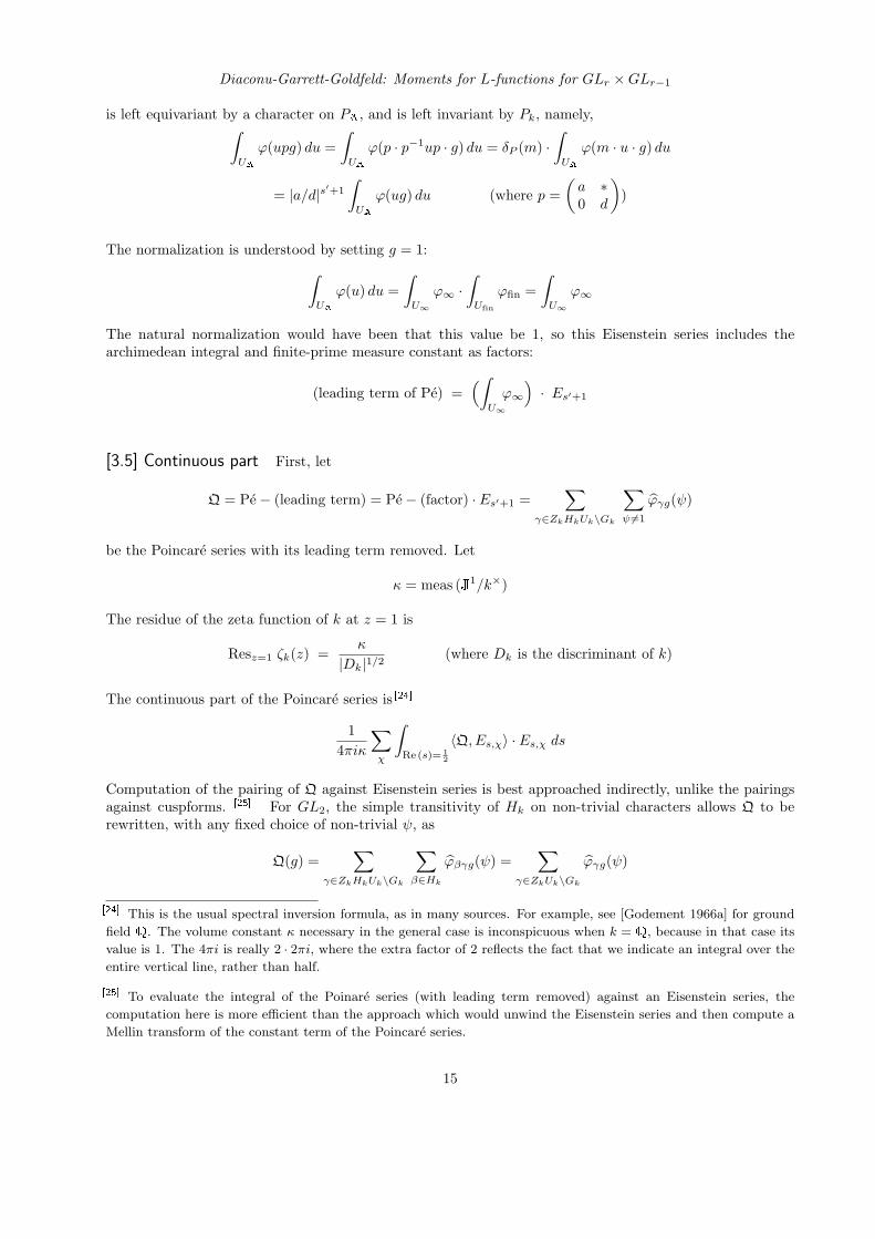
is left equivariant by a character on PA, and is left invariant by Pk, namely,∫UA

ϕ(upg) du =∫UA

ϕ(p · p−1up · g) du = δP (m) ·∫UA

ϕ(m · u · g) du

= |a/d|s′+1

∫UA

ϕ(ug) du (where p =(a ∗0 d

))

The normalization is understood by setting g = 1:∫UA

ϕ(u) du =∫U∞

ϕ∞ ·∫Ufin

ϕfin =∫U∞

ϕ∞

The natural normalization would have been that this value be 1, so this Eisenstein series includes thearchimedean integral and finite-prime measure constant as factors:

(leading term of Pe) =(∫

U∞

ϕ∞

)· Es′+1

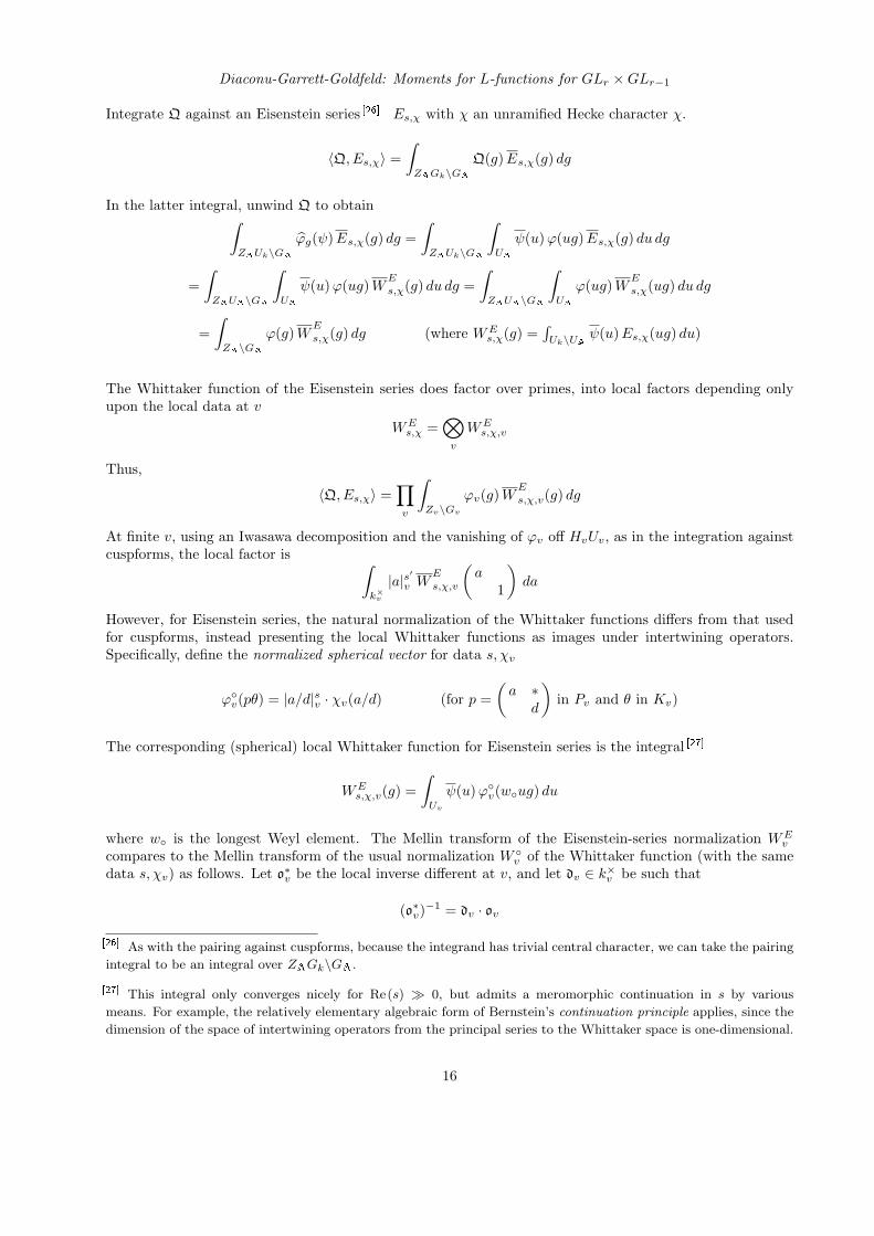
[3.5] Continuous part First, let

Q = Pe− (leading term) = Pe− (factor) · Es′+1 =∑

γ∈ZkHkUk\Gk

∑ψ 6=1

ϕγg(ψ)

be the Poincare series with its leading term removed. Let

κ = meas (J1/k×)

The residue of the zeta function of k at z = 1 is

Resz=1 ζk(z) =κ

|Dk|1/2(where Dk is the discriminant of k)

The continuous part of the Poincare series is [24]

14πiκ

∑χ

∫Re(s)= 1

2

〈Q, Es,χ〉 · Es,χ ds

Computation of the pairing of Q against Eisenstein series is best approached indirectly, unlike the pairingsagainst cuspforms. [25] For GL2, the simple transitivity of Hk on non-trivial characters allows Q to berewritten, with any fixed choice of non-trivial ψ, as

Q(g) =∑

γ∈ZkHkUk\Gk

∑β∈Hk

ϕβγg(ψ) =∑

γ∈ZkUk\Gk

ϕγg(ψ)

[24] This is the usual spectral inversion formula, as in many sources. For example, see [Godement 1966a] for ground

field Q. The volume constant κ necessary in the general case is inconspicuous when k = Q, because in that case its

value is 1. The 4πi is really 2 · 2πi, where the extra factor of 2 reflects the fact that we indicate an integral over the

entire vertical line, rather than half.

[25] To evaluate the integral of the Poinare series (with leading term removed) against an Eisenstein series, the

computation here is more efficient than the approach which would unwind the Eisenstein series and then compute a

Mellin transform of the constant term of the Poincare series.

15


Integrate Q against an Eisenstein series [26] Es,χ with χ an unramified Hecke character χ.

〈Q, Es,χ〉 =∫ZAGk\GA

Q(g)Es,χ(g) dg

In the latter integral, unwind Q to obtain∫ZAUk\GA

ϕg(ψ)Es,χ(g) dg =∫ZAUk\GA

∫UA

ψ(u)ϕ(ug)Es,χ(g) du dg

=∫ZAUA\GA

∫UA

ψ(u)ϕ(ug)WE

s,χ(g) du dg =∫ZAUA\GA

∫UA

ϕ(ug)WE

s,χ(ug) du dg

=∫ZA\GA

ϕ(g)WE

s,χ(g) dg (where WEs,χ(g) =

∫Uk\UA ψ(u)Es,χ(ug) du)

The Whittaker function of the Eisenstein series does factor over primes, into local factors depending onlyupon the local data at v

WEs,χ =

⊗v

WEs,χ,v

Thus,

〈Q, Es,χ〉 =∏v

∫Zv\Gv

ϕv(g)WE

s,χ,v(g) dg

At finite v, using an Iwasawa decomposition and the vanishing of ϕv off HvUv, as in the integration againstcuspforms, the local factor is ∫

k×v

|a|s′

v WE

s,χ,v

(a

1

)da

However, for Eisenstein series, the natural normalization of the Whittaker functions differs from that usedfor cuspforms, instead presenting the local Whittaker functions as images under intertwining operators.Specifically, define the normalized spherical vector for data s, χv

ϕ◦v(pθ) = |a/d|sv · χv(a/d) (for p =(a ∗

d

)in Pv and θ in Kv)

The corresponding (spherical) local Whittaker function for Eisenstein series is the integral [27]

WEs,χ,v(g) =

∫Uv

ψ(u)ϕ◦v(w◦ug) du

where w◦ is the longest Weyl element. The Mellin transform of the Eisenstein-series normalization WEv

compares to the Mellin transform of the usual normalization W ◦v of the Whittaker function (with the samedata s, χv) as follows. Let o∗v be the local inverse different at v, and let dv ∈ k×v be such that

(o∗v)−1 = dv · ov

[26] As with the pairing against cuspforms, because the integrand has trivial central character, we can take the pairing

integral to be an integral over ZAGk\GA.

[27] This integral only converges nicely for Re(s) � 0, but admits a meromorphic continuation in s by various

means. For example, the relatively elementary algebraic form of Bernstein’s continuation principle applies, since the

dimension of the space of intertwining operators from the principal series to the Whittaker space is one-dimensional.

16


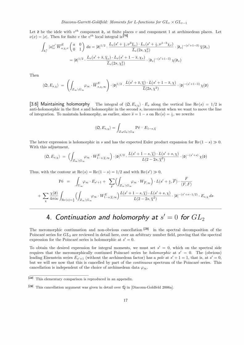
Let d be the idele with vth component dv at finite places v and component 1 at archimedean places. Letν(x) = |x|. Then for finite v the vth local integral is [28]∫

k×v

|a|s′

v WE

s,χ,v

(a 00 1

)da = |d|1/2 · Lv(s

′ + 12 , ν

sχv) · Lv(s′ + 12 , ν

1−sχv)Lv(2s, χ2

v)· |dv|−(s′+1−s) χ(dv)

= |d|1/2 · Lv(s′ + s, χv) · Lv(s′ + 1− s, χv)

Lv(2s, χ2v)

· |dv|−(s′+1−s) χ(dv)

Then

〈Q, Es,χ〉 =

(∫Z∞\G∞

ϕ∞ ·WE

s,χ,∞

)· |d|1/2 · L(s′ + s, χ) · L(s′ + 1− s, χ)

L(2s, χ2)· |d|−(s′+1−s) χ(d)

[3.6] Maintaining holomorphy The integral of 〈Q, Es,χ〉 · Es along the vertical line Re(s) = 1/2 isanti-holomorphic in the first s and holomorphic in the second s, inconvenient when we want to move the lineof integration. To maintain holomorphy, as earlier, since s = 1− s on Re(s) = 1

2 , we rewrite

〈Q, Es,χ〉 =∫ZAGk\GA

Pe · E1−s,χ

The latter expression is holomorphic in s and has the expected Euler product expansion for Re(1− s)� 0.With this adjustment,

〈Q, Es,χ〉 =(∫

Z∞\G∞ϕ∞ ·WE

1−s,χ,∞

)· |d|1/2 · L(s′ + 1− s, χ) · L(s′ + s, χ)

L(2− 2s, χ2)· |d|−(s′+s) χ(d)

Thus, with the contour at Re(s) = Re(1− s) = 1/2 and with Re(s′)� 0,

Pe =∫U∞

ϕ∞ · Es′+1 +∑F

(∫Z∞\G∞

ϕ∞ ·WF,∞

)· L(s′ + 1

2 , F ) · F

〈F, F 〉

+∑χ

χ(d)4πiκ

∫Re(s)= 1

2

(∫Z∞\G∞

ϕ∞ ·WE1−s,χ,∞

)L(s′ + 1− s, χ) · L(s′ + s, χ)L(2− 2s, χ2)

· |d|−(s′+s−1/2) · Es,χ ds

4. Continuation and holomorphy at s′ = 0 for GL2

The meromorphic continuation and non-obvious cancellation [29] in the spectral decomposition of thePoincare series for GL2 are reviewed in detail here, over an arbitrary number field, proving that the spectralexpression for the Poincare series is holomorphic at s′ = 0.

To obtain the desired expression for integral moments, we must set s′ = 0, which on the spectral siderequires that the meromorphically continued Poincare series be holomorphic at s′ = 0. The (obvious)leading Eisenstein series Es′+1 (without the archimedean factor) has a pole at s′ + 1 = 1, that is, at s′ = 0,but we will see now that this is cancelled by part of the continuous spectrum of the Poincare series. Thiscancellation is independent of the choice of archimedean data ϕ∞.

[28] This elementary comparison is reproduced in an appendix.

[29] This cancellation argument was given in detail over Q in [Diaconu-Goldfeld 2006a].

17


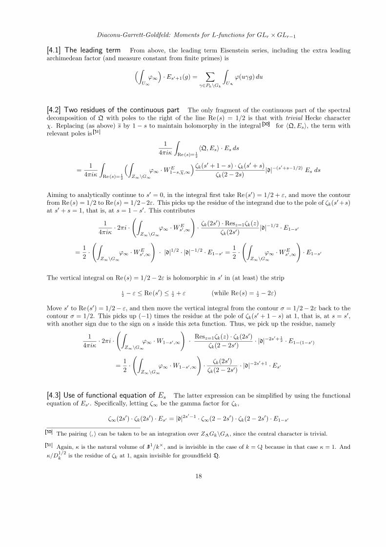
[4.1] The leading term From above, the leading term Eisenstein series, including the extra leadingarchimedean factor (and measure constant from finite primes) is(∫

U∞

ϕ∞

)· Es′+1(g) =

∑γ∈Pk\Gk

∫UA

ϕ(uγg) du

[4.2] Two residues of the continuous part The only fragment of the continuous part of the spectraldecomposition of Q with poles to the right of the line Re(s) = 1/2 is that with trivial Hecke characterχ. Replacing (as above) s by 1 − s to maintain holomorphy in the integral [30] for 〈Q, Es〉, the term withrelevant poles is [31]

14πiκ

∫Re(s)= 1

2

〈Q, Es〉 · Es ds

=1

4πiκ

∫Re(s)= 1

2

(∫Z∞\G∞

ϕ∞ ·WE1−s,χ,∞

)ζk(s′ + 1− s) · ζk(s′ + s)ζk(2− 2s)

|d|−(s′+s−1/2) Es ds

Aiming to analytically continue to s′ = 0, in the integral first take Re(s′) = 1/2 + ε, and move the contourfrom Re(s) = 1/2 to Re(s) = 1/2−2ε. This picks up the residue of the integrand due to the pole of ζk(s′+s)at s′ + s = 1, that is, at s = 1− s′. This contributes

14πiκ

· 2πi ·

(∫Z∞\G∞

ϕ∞ ·WEs′,∞

)· ζk(2s′) · Resz=1ζk(z)

ζk(2s′)|d|−1/2 · E1−s′

=12·

(∫Z∞\G∞

ϕ∞ ·WEs′,∞

)· |d|1/2 · |d|−1/2 · E1−s′ =

12·

(∫Z∞\G∞

ϕ∞ ·WEs′,∞

)· E1−s′

The vertical integral on Re(s) = 1/2− 2ε is holomorphic in s′ in (at least) the strip

12 − ε ≤ Re(s′) ≤ 1

2 + ε (while Re(s) = 12 − 2ε)

Move s′ to Re(s′) = 1/2− ε, and then move the vertical integral from the contour σ = 1/2− 2ε back to thecontour σ = 1/2. This picks up (−1) times the residue at the pole of ζk(s′ + 1− s) at 1, that is, at s = s′,with another sign due to the sign on s inside this zeta function. Thus, we pick up the residue, namely

14πiκ

· 2πi ·

(∫Z∞\G∞

ϕ∞ ·W1−s′,∞

)· Resz=1ζk(z) · ζk(2s′)

ζk(2− 2s′)· |d|−2s′+ 1

2 · E1−(1−s′)

=12·

(∫Z∞\G∞

ϕ∞ ·W1−s′,∞

)· ζk(2s′)ζk(2− 2s′)

· |d|−2s′+1 · Es′

[4.3] Use of functional equation of Es The latter expression can be simplified by using the functionalequation of Es′ . Specifically, letting ζ∞ be the gamma factor for ζk,

ζ∞(2s′) · ζk(2s′) · Es′ = |d|2s′−1 · ζ∞(2− 2s′) · ζk(2− 2s′) · E1−s′

[30] The pairing 〈, 〉 can be taken to be an integration over ZAGk\GA, since the central character is trivial.

[31] Again, κ is the natural volume of J1/k×, and is invisible in the case of k = Q because in that case κ = 1. And

κ/D1/2k is the residue of ζk at 1, again invisible for groundfield Q.

18


In the situation at hand, this gives

ζk(2s′)ζk(2− 2s′)

· Es′ = |d|2s′−1 · ζ∞(2− 2s′)

ζ∞(2s′)· E1−s′

Thus, the powers of |d| cancel, and the second residue can be rewritten as

12·

(∫Z∞\G∞

ϕ∞ ·W1−s′,∞

)· ζ∞(2− 2s′)

ζ∞(2s′)· E1−s′

These two contributions from the continuous part are

12 ·

(∫Z∞\G∞

ϕ∞ ·[Ws′,∞ +

ζ∞(2− 2s′)ζ∞(2s′)

·W1−s′,∞

])· E1−s′

[4.4] Use of functional equation of archimedean Whittaker functions The archimedean-place(and finite-prime) Whittaker functions are normalized by presenting the Whittaker functions by the usualintertwining integral (and analytically continuing), as follows. Let

ηs(umθ) = |a/d|sv (for u ∈ U , m =(a

d

), θ ∈ Kv)

The normalization of the Whittaker function is

WEs,v(g) =

∫Uv

ψ(u) ηs(w◦ug) du (for Re(s)� 0, fixed non-trivial ψ)

Further, for v archimedean

WEs,v

(a

1

)=∫kv

ψ0(x)∣∣∣∣ a

aaι + xxι

∣∣∣∣sv

dx = |a|1−sv

∫kv

ψ0(ax)1

|1 + xxι|svdx

by replacing x by ax, where ι is complex conjugation for v ≈ C and is the identity map for v ≈ R. Theusual computation shows that

WEs,R

(a

1

)=|a|1/2

π−sΓ(s)

∫ ∞0

e−π(t+ 1t )|a| ts−

12dt

t=

1ζR(2s)

× (invariant under s↔ 1− s)

and, similarly, [32]

WEs,C

(a

1

)=

|a|(2π)−2sΓ(2s)

∫ ∞0

e−2π(t+ 1t )|a| t2s−1 dt

t=

1ζC(2s)

× (invariant under s↔ 1− s)

Thus, in both cases,

ζv(2− 2s)ζv(2s)

·WE1−s,v

(a

1

)= WE

s,v

(a

1

)(for v archimedean)

[32] In the displayed identity for v ≈ C, an unadorned absolute value is not |x|C = xxι, but, rather, the standard

|x| =√xxι. The appropriate measure is double the usual.

19


and

WE1−s =

ζ∞(2s)ζ∞(2− 2s)

·WEs

Thus, in fact, the second of the two residues from the continuous part is identical to the first. Thus, thesetwo residues combine to give (∫

Z∞\G∞ϕ∞ ·Ws′,∞

)· E1−s′

Thus, to prove that the leading term’s pole at s′ = 0 is cancelled by the poles of these residues at s′ = 0, wemust show that(∫

U∞

ϕ∞

)· E1+s′ +

(∫Z∞\G∞

ϕ∞ ·Ws′,∞

)· E1−s′ = (holomorphic at s′ = 0)

[4.5] Invocation of Fourier inversion Thus, to prove cancellation of poles at s′ = 0 it suffices to provea local fact, namely, that∫

Uv

ϕv =(∫

Zv\Gvϕv ·WE

s′,v

) ∣∣∣s′=0

(for all archimedean v)

The Whittaker function WEs,v can be presented in terms of a Fourier transform

WEs,v

(a

1

)= |a|1−s · Ψs,v(a) (where Ψ(x) = Ψs(x) = |1 + xxι|−sv , v archimedean)

Let

Φ(x) = ϕv

(1 x

1

)Using the right Kv-invariance and an Iwasawa decomposition, and noting that Φ and Ψ are even,∫

Zv\Gvϕv ·WE

s′,v =∫k×v

∫kv

|a|s′Φ(x) · |a|1−s

′Ψ(a)ψ(ax) dx da

=∫k×v

Φ(a) Ψ(a) |a| da =∫k×v

Φ(a) Ψ(a) |a| da

by Fourier inversion, since |a|da is an additive Haar measure. Writing the latter expression out, it is∫kv

ϕv

(1 a

1

)· 1|1 + aaι|s′v

|a| da

The equality ∫Zv\Gv

ϕv ·WEs′,v =

∫k×v

ϕv

(1 a

1

)· 1|1 + aaι|s′v

|a| da

holds at first only for Re(s′) � 0, but then extends by analytic continuation for ϕv sufficiently integrableon Nv. Thus, we can evaluate the latter integral at s′ = 0, obtaining∫

Zv\Gvϕv ·WE

0,v =∫k×v

ϕv

(1 a

1

)|a| da

20


At archimedean places v, the normalization |a| da for an additive Haar measure, in terms of a multiplicativeHaar measure da, is correct. This proves that, indeed,(∫

Zv\Gvϕv ·WE

s′,v

) ∣∣∣s′=0

=∫Uv

ϕv (for all archimedean v)

which yields the desired cancellation.

5. Spectral expansion for GLr

The spectral decomposition of the Poincare series for r = 2 yields that for r > 2 by inducing. For r > 2,nothing remains after all the non-L2 terms are removed. The non-L2 terms are induced from the genuinelyL2 spectral expansion of the Poincare series on GL2.

Before carrying out the spectral expansion for r = 2, we had found that

Pe(g) =(∫

U∞

ϕ∞

)· Er+1,1

s′+1 (g) +∑

γ∈P r−2,2k \Gk

Φ(γg)

where

Φ(A ∗

D

)= |detA|s

′+1 · | detD|− (r−2)· s′+12 ·Q(

rs′ + r − 22

, ϕ,D) (with A ∈ GLr−2 and D ∈ GL2)

with Q from GL2, and

ϕ(g) =∫U ′k\U

′A

ϕ(u′g) du′

Thus, formation of Pe (with its leading term removed) amounts to forming an Eisenstein series from Φ, withanalytical properties explicated by expressing Φ as a superposition of vectors generating irreducibles.

[5.1] Decomposition into irreducibles

From the decomposition of Q on GL2 for Re(s′)� 0

Φ(A ∗0 D

)= |detA|2·

s′+12 · | detD|− (r−2)· s

′+12 ·Q(

rs′ + r − 22

, ϕ,D)

= |detA|2·s′+1

2 · | detD|− (r−2)· s′+12

∑F

(∫PGL2(k∞ )

ϕ∞ ·WF,∞

)· L(

rs′ + r − 22

+ 12 , F ) · F

〈F, F 〉

+ |detA|2·s′+1

2 · | detD|− (r−2)· s′+12

∑χ

χ(d)4πiκ

∫Re(s)= 1

2

(∫PGL2(k∞)

ϕ∞ ·WE1−s,χ,∞

)·L( rs

′+r−22 + 1− s, χ) · L( rs

′+r−22 + s, χ)

L(2− 2s, χ2)·|d|−( rs

′+r−22 +s−1/2) ·Es,χ(D) ds

[5.2] Least continuous part of Poincare series

Let

Φ s′+12 ,F

((A ∗0 D

)· θ) = |detA|2·

s′+12 · | detD|− (r−2)· s

′+12 F (D) (for θ ∈ KA)

21


and define a half-degenerate Eisenstein series [33]

Er−2,2s′+1

2 ,F(g) =

∑γ∈P r−2,2

k \Gk

Φ s′+12 ,F

(γg)

Then the most-cuspidal (or least continuous) part of the Poincare series is

∑F

(∫PGL2(k∞)

ϕ ·WF,∞

)·L( rs

′+r−22 + 1

2 , F )〈F, F 〉

· Er−2,2s′+1

2 ,F(cuspforms F on GL2)

The summands of this expression have relatively well understood meromorphic continuations. As discussedin an appendix, the half-degenerate Eisenstein series Er−2,2

s,F has no poles in Re(s) ≥ 1/2. With s = (s′+1)/2this assures absence of poles in Re(s′) ≥ 0.

[5.3] Continuous part of the Poincare series The Eisenstein series integral part of Q on GL2 givesdegenerate Eisenstein series attached to the (r − 2, 1, 1)-parabolic in GLr. This arises from a similarconsideration as for GL2 cuspforms, but for GL2 Eisenstein series, as follows.

Let Es,χ be the usual Eisenstein series for GL2, and let

Φ s′+12 ,Es,χ

((A ∗0 D

)· θ) = |detA|2·

s′+12 · | detD|− (r−2)· s

′+12 Es,χ(D) (for θ ∈ KA)

and define an Eisenstein series

Er−2,2s′+1

2 ,Es,χ(g) =

∑γ∈P r−2,2

k \Gk

Φ s′+12 ,Es,χ

(γg)

For given s ∈ C, an easy variant of Godement’s criterion [34] proves convergence for sufficiently large Re(s′).

Then, ignoring the issue of interchange of sums and integrals, the Poincare series has most continuous part∑χ

χ(d)4πiκ

∫Re(s)= 1

2

(∫PGL2(k∞)

ϕ∞ ·WE1−s,χ,∞

)

×L( rs

′+r−22 + 1− s, χ) · L( rs

′+r−22 + s, χ)

L(2− 2s, χ2)· |d|−( rs

′+r−22 +s−1/2) · Er−2,2

s′+12 ,Es,χ

ds

That is, it is the analytically continued Es on the line Re(s) = 12 that enters. However, as usual, for

Re(s) � 0 and Re(s′) � 0 this iterated formation of Eisenstein series is equal to a single-step Eisensteinseries. The equality persists after analytic continuation.

Thus, let

Φs1,s2,s3,χ(

A ∗ ∗0 m2 ∗0 0 m3

· θ)= |detA|s1 · |m2|s2χ(m2) · |m3|s3χ(m3) (for θ ∈ KA and A ∈ GLr−2)

[33] Visibly, this Eisenstein series is a P r−2,2 Eisenstein series degenerate on the (upper-left) Levi component GLr−2

for r > 3, while cuspidal on the (lower-right) Levi component GL2. Basic analytic properties of such Eisenstein series

are accessible by relatively elementary methods, as noted in the appendix on half-degenerate Eisenstein series.

[34] A neo-classical version of Godement’s criterion is in [Borel 1966].

22


andEr−2,1,1s1,s2,s3,χ =

∑γ∈P r−2,1,1

k \Gk

Φs1,s2,s3,χ(γg)

Then, ignoring the issue of interchange of sums and integrals, the Poincare series has most continuous part∑χ

χ(d)4πiκ

∫Re(s)= 1

2

(∫PGL2(k∞)

ϕ∞ ·WE1−s,χ,∞

)

×L( rs

′+r−22 + 1− s, χ) · L( rs

′+r−22 + s, χ)

L(2− 2s, χ2)· |d|−( rs

′+r−22 +s−1/2) · Er−2,1,1

2· s′+12 , s−(r−2)· s′+1

2 , −s−(r−2)· s′+12 , χ

ds

[5.4] Comment It is remarkable that there are no further terms in the spectral expansion of Pe, beyondthe main term, the cuspidal GL2 part induced up to GLr, and the continuous GL2 part induced up to GLr.

6. Continuation and cancellation for GLr

Take r > 2. In meromorphically continuing the Poincare series to s′ = 0 the leading term(∫U∞

ϕ∞

)· Er+1,1

s′+1 (g)

seems to create an obstruction, having a pole at s′ = 0 (coming from the pole of the Eisenstein series). Aswith GL2, it is not obvious, but this pole is cancelled by poles coming from the trivial-χ integral of Eisensteinseries

14πiκ

∫Re(s)= 1

2

(∫PGL2(k∞)

ϕ∞(rs′ + r − 2

2) ·WE

1−s,∞

)

×ζ( rs

′+r−22 + 1− s) · ζ( rs

′+r−22 + s)

ζ(2− 2s)· |d|−( rs

′+r−22 +s−1/2) · Er−2,1,1

2· s′+12 , s−(r−2)· s′+1

2 , −s−(r−2)· s′+12

ds

Unlike the GL2 case, for r > 2 the relevant poles of this integral are due to the Eisenstein series, not to thezeta functions.

[6.1] Residue of leading term First, recall from the appendix that the leading term has residue at s′ = 0given explicitly by the residue of the Eisenstein series, namely [35]

Ress′=0

(∫U∞

ϕ∞

)· Er+1,1

s′+1 (g) =(∫

U∞

ϕ∞

)· Ress′=0E

r+1,1s′+1 (g) =

(∫U∞

ϕ∞

)· κ · |d|

r/2

r · ξ(r)

[6.2] The initial situation The spectral decomposition initially holds for Re(s′) � 0 while the integral

[35] As usual, the function ξ(s) is the zeta function of the underlying number field with gamma factors added, but

not attempting to compensate for the conductor or epsilon factor (the latter being absent here). Thus, the functional

equation is

ξ(s) = |d|1/2 · |d|−(1−s) · ξ(1− s) = |d|s−12 · ξ(1− s)

where d is a finite idele generating the local different everywhere. The first |d|1/2 is the product of standard measures

of local integers at ramified primes, and |d|−(1−s) arises because the Fourier transform of the characteristic function

of the local integers is the characteristic function of the local inverse different.

23


is along Re(s) = 1/2. For brevity, let the three complex arguments to the Eisenstein series be denoted

s1 = 2 · s′ + 12

s2 = s− (r − 2)s′ + 1

2s3 = −s− (r − 2)

s′ + 12

For Re(s′) � 0, certainly Re(s1 − s2) > r − 1 and Re(s1 − s3) > r, although Re(s2 − s3) = 1, sinceRe(s) = 1/2. Thus, for convergence, the Eisenstein series Er−2,1,1

s1,s2,s3 must be understood as formed by inducingup along P r−2,2 the meromorphic continuation of E1,1

s2,s3 . Godement’s criterion [36] yields convergence.

[6.3] Move s′ to the left edge Aiming to move s′ toward 0, first move s′ as far to the left as possiblewithout violating either of the two conditionsRe(s1 − s2) > r − 1 (first condition)

Re(s1 − s3) > r (second condition)

Let σ = Re(s) and σ′ = Re(s′). Expanded, the first condition is

2 · σ′ + 12−(σ − (r − 2) · σ

′ + 12

)> r − 1

which simplifies to

r · σ′ + 12

> σ + r − 1

and thenσ′ + 1

2>σ

r+ 1− 1

r

and finally

σ′ > 1− 2(1− σ)r

(first condition, simplified)

Similarly, the second condition becomes

σ′ > 1− 2σr

(second condition, simplified)

For σ = Re(s) = 1/2, which is where we start, these two conditions are equivalent, namely

σ′ > 1− 1r

(either condition, at σ = 12 )

Thus, move s′ close to the left edge of the region defined by these conditions: for small ε > 0 move σ′ = Re(s′)to σ′ = 1− 1

r + ε.

[6.4] First contour shift and residue Now solve the two inequalities for σ in terms of σ′. These areσ < r2 · σ

′ − r−22 (first condition, rearranged)

σ > − r2 · σ′ + r

2 (second condition, rearranged)

With σ′ = 1− 1r + ε, move σ to the left, from 1

2 to 12 −

r+12 ε. This causes the second condition (but not the

first) to be violated:12 −

r+12 · ε < 1

2 + r2 · ε = r

2 · (1−1r + ε)− r−2

2 (first condition holds)

12 −

r+12 · ε 6> 1

2 −r2 · ε = − r2 · (1−

1r + ε) + r

2 (second condition fails)

[36] A neo-classical version of Godement’s criterion appears in [Borel 1966].

24


Thus, we pick up 2πi times the residue of the pole of the Eisenstein series at

s = − r

2· s′ + r

2=r

2· (1− s′)

The corresponding residue of the P r−2,1,1 Eisenstein series is (from the appendix)

κ · |d| r−12

ξ(r − 1)· ξ(s2 − s3 − 1)

ξ(s2 − s3)· Er−1,1

s1−1,s2−1

=κ · |d| r−1

2

ξ(r − 1)· ξ(r(1− s

′)− 1)ξ(r(1− s′))

· Er−1,1s′,−(r−1)s′

With s = r(1− s′)/2, the zeta functions in the integral of Eisenstein series become

ζ( rs′+r−2

2 + 1− r2 (1− s′)) · ζ( rs

′+r−22 + r

2 (1− s′))ζ(2− r(1− s′))

=ζ(rs′) · ζ(r − 1)ζ(2− r + rs′)

That is, apart from the 2πi and archimedean factor, we have picked up

(2πi) · ζ(rs′) · ζ(r − 1)ζ(2− r + rs′)

· κ · |d|r−1

2

ξ(r − 1)· ξ(r(1− s

′)− 1)ξ(r(1− s′))

· Er−1,1s′

From the appendix,Res′=0 ξ(rs′) · Er−1,1

s′ = − κ

r

The only other finite-prime zeta which misbehaves at s′ = 0 is the ζ(2− r + rs′) in the denominator. Fromthe functional equation

ζ(s) =ξ(s)ζ∞(s)

=|d|s− 1

2 · ξ(1− s)ζ∞(s)

we have

1ζ(2− r + rs′)

= |d| 12−(2−r+rs′) · ζ∞(2− r + rs′)ξ(1− (2− r + rs′))

= |d| 12−2+r−rs′ · ζ∞(2− r + rs′)ξ(r − 1− rs′)

Thus, the iterated residue at s′ = 0 of this residue (without 2πi and without the archimedean factor) is

Ress′=0

(ζ∞(2− r + rs′)

ζ∞(rs′)

)· ζ(r − 1) · κ · |d| 3r2 −2 · ξ(r − 1)

ξ(r − 1) · ξ(r − 1) · ξ(r)·(− κ

r

)

= −Ress′=0

(ζ∞(2− r + rs′)

ζ∞(rs′)

)· κ · |d| 3r2 −2

ζ∞(r − 1) · ξ(r)·(κr

)

[6.5] The archimedean factor Takes =

r

2· (1− s′)

and use the functional equation for the GL2 archimedean Whittaker function, namely

WE1−s =

ζ∞(2s)ζ∞(2− 2s)

·WEs

Then the archimedean integral is∫PGL2(k∞)

ϕ∞(rs′ + r − 2

2) · ζ∞(r · (1− s′))ζ∞(2− r · (1− s′))

·WEr2 (1−s′),∞

25


Continuing this discussion shows that the continuous-spectrum part of the spectral decomposition cancelsthe pole of the singular term, giving the meromorphic continuation to s′ = 0.

7. Appendix: half-degenerate Eisenstein series

Take q > 1, and let f be a cuspform on GLq(A), in the strong sense that f is in L2(GLq(k)\GLq(A)1), andf meets the Gelfand-Fomin-Graev conditions∫

Nk\NAf(ng) dn = 0 (for almost all g)

and f generates an irreducible representation of GLq(kν) locally at all places ν of k. For a Schwartz functionΦ on Aq×r and Hecke character χ, let

ϕ(g) = ϕχ,f,Φ(g) = χ(det g)q∫GLq(A)

f(h−1)χ(deth)r Φ(h · [0q×(r−q) 1q] · g) dh

This function ϕ has the same central character as f . It is left invariant by the adele points of the unipotentradical

N = {(

1r−q ∗1r

)} (unipotent radical of P = P r−q,q)

The function ϕ is left invariant under the k-rational points Mk of the standard Levi component of P ,

M = {(a

d

): a ∈ GLr−q, d ∈ GLr}

To understand the normalization, observe that

ξ(χr, f,Φ(0, ∗)) = ϕ(1) =∫GLq(A)

f(h−1)χ(deth)r Φ(h · [0q×(r−q) 1q]) dh

is a zeta integral as in [Godement-Jacquet 1972] for the standard L-function attached to the cuspform f (orperhaps a contragredient). Thus, the Eisenstein series formed from ϕ includes this zeta integral as a factor,so write

ξ(χr, f,Φ(0, ∗)) · EPχ,f,Φ(g) =∑

γ∈Pk\GLr(k)

ϕ(γ g) (convergent for Re(χ) >> 0)

Now prove the meromorphic continuation via Poisson summation:

ξ(χr, f,Φ(0, ∗)) · EPχ,f,Φ(g)

= χ(det g)q∑

γ∈Pk\GLr(k)

∫GLq(k)\GLq(A)

f(h)χ(deth)−r∑

α∈GLq(k)

Φ(h−1 · [0 α] · g) dh

= χ(det g)q∫GLq(k)\GLq(A)

f(h)χ(deth)−r∑

y∈kq×r, full rank

Φ(h−1 · y · g) dh

The Gelfand-Fomin-Graev condition on f will compensate for the otherwise-irksome full-rank constraint.Anticipating that we can drop the rank condition suggests that we define

ΘΦ(h, g) =∑

y∈kq×rΦ(h−1 · y · g)

26


As in [Godement-Jacquet 1972], the non-full-rank terms integrate to 0: [37]

[7.0.1] Proposition: For f a cuspform, less-than-full-rank terms integrate to 0, that is,∫GLq(k)\GLq(A)

f(h)χ(deth)−r∑

y∈kq×r, rank <q

Φ(h−1 · y · g) dh = 0

Proof: Since this is asserted for arbitrary Schwartz functions Φ, we can take g = 1. By linear algebra, giveny0 ∈ kq×r of rank `, there is α ∈ GLq(k) such that

α · y0 =(

y`×r0(q−`)×r

)(with `-by-r block y`×r of rank `)

Thus, without loss of generality fix y0 of the latter shape. Let Y be the orbit of y0 under left multiplicationby the rational points of the parabolic

P `,q−` = {(`-by-` ∗

0 (q − `)-by-(q − `)

)} ⊂ GLq

This is some set of matrices of the same shape as y0. Then the subsum over GLq(k) · y0 is∫GLq(k)\GLq(A)

f(h)χ(deth)−r∑

y∈GLq(k)·y0

Φ(h−1 · y) dh =∫P `,q−`k \GLq(A)

f(h)χ(deth)−r∑y∈Y

Φ(h−1 · y) dh

Let N and M be the unipotent radical and standard Levi component of P `,q−`,

N =(

1` ∗0 1q−`

)M =

(`-by-` 0

0 (q − `)-by-(q − `)

)Then the integral can be rewritten as an iterated integral∫

NkMk\GLq(A)

f(h)χ(deth)−r∑y∈Y

Φ(h−1 · y) dh

=∫NAMk\GLq(A)

∑y∈Y

∫Nk\NA

f(nh)χ(detnh)−r Φ((nh)−1 · y) dn dh

=∫NAMk\GLq(A)

∑y∈Y

χ(deth)−r Φ(h−1 · y)

(∫Nk\NA

f(nh) dn

)dh

[37] There are issues of convergence. First, for Re(χ) sufficiently large, the integral

χ(det g)qX

γ∈Pk\GLr(k)

ZGLq(k)\GLq(A)

f(h)χ(deth)−r Θ(h, g) dh

is absolutely convergent. Also, we have the integrals analogous to integrals over k×\J+. That is, let

GL+q = {h ∈ GLq(A) : | deth| ≥ 1}. Then, for arbitrary χ, using the fact that cuspforms f are of rapid decay

in Siegel sets,

χ(det g)qX

γ∈Pk\GLr(k)

ZGLq(k)\GL+

q

f(h)χ(deth)−rX

y∈kq×r, full rank

Φ(h−1 · y · g) dh

is absolutely convergent.

27


since all fragments but f(nh) in the integrand are left invariant by NA. But the inner integral of f(nh) is0, by the Gelfand-Fomin-Graev condition, so the whole is 0. ///

Let ι denote the transpose-inverse involution(s). Poisson summation gives

ΘΦ(h, g) =∑

y∈kq×rΦ(h−1 · y · g)

= |det(h−1)ι|r |det gι|q∑

y∈kq×rΦ((hι)−1 · y · gι) = |det(h−1)ι|r |det gι|q ΘbΦ(hι, gι)

As with ΘΦ, the not-full-rank summands in ΘbΦ integrate to 0 against cuspforms. Thus, letting

GL+q = {h ∈ GLq(A) : |deth| ≥ 1} GL−q = {h ∈ GLq(A) : |deth| ≤ 1}

ξ(χr, f,Φ(0, ∗)) · EPχ,f,Φ(g) = χ(det g)q∫GLq(k)\GLq(A)

f(h)χ(deth)−r ΘΦ(h, g) dh

= χ(det g)q∫GLq(k)\GL+

q

f(h)χ(deth)−r ΘΦ(h, g) dh+ χ(det g)q∫GLq(k)\GL−q


= χ(det g)q∫GLq(k)\GL+

q


+ χ(det g)q∫GLq(k)\GL−q

|det(h−1)ι|r |det gι|q f(h)χ(deth)−r ΘbΦ(hι, gι) dh

By replacing h by hι in the second integral, convert it to an integral over GLq(k)\GL+q , and the whole is

ξ(χr, f,Φ(0, ∗)) · EPχ,f,Φ(g) = χ(det g)q∫GLq(k)\GL+

q


+ νχ−1(det gι)q∫GLq(k)\GL+

q

f(hι) νχ−1(dethι)−r ΘbΦ(h, gι) dh

Since f ◦ ι is a cuspform, the second integral is entire in χ. Thus, we have proven

ξ(χr, f,Φ(0, ∗)) · EPχ,f,Φ is entire

[7.1] Remark Except for the extreme case q = r− 1, these Eisenstein series are degenerate, so occur onlyas (iterated) residues of cuspidal-data Eisenstein series. Assessing poles of residues is less effective in thepresent special circumstances than the above argument.

8. Appendix: Eisenstein series for GL2

We compute Mellin transforms of the Whittaker functions attached to Eisenstein series for GL2 (with trivialcentral character, spherical, over a number field k). The natural normalization of Eisenstein series adds afurther local L-factor to the Mellin transform (as well as a measure constant at ramified primes), by contrastto the usual Mellin transform of the usual normalization W ◦v of the spherical Whittaker function. And atthe end we give a precise function equation.

[8.1] The standard Eisenstein series Let G = GL2 and

P = {(∗ ∗0 ∗

)} N = {

(1 ∗0 1

)} M = {

(∗ 00 1

)}

28


and let Z be the center. An absolutely unramified Hecke character can be decomposed as χ(α) · |α|scorresponding to the usual decomposition

J/k× ≈ J1/k× × (0,+∞)

The standard normalization of the spherical function (in the tensor product of principal series) is ϕ =⊗

v ϕvwith

ϕv((a ∗0 1

)· θ) = |a/d|sv · χv(a/d) (θ in the standard maximal compact of GL2(kv))

Thus, ϕv(1) = 1 for all v. The standard Eisenstein series attached to data s, χ is

E(g) = Es,χ(g) =∑Pk\Gk

ϕ(γg)

[8.2] The Eisenstein Whittaker functions Let ψ be the standard non-trivial character on A/k. Let ovbe the local integers at a finite place v, let p be the rational prime lying under v. The dual lattice to ov withrespect to trace is

o∗v = {α ∈ kv : tr kvQp(αβ) ∈ Zp : for all β ∈ ov}

This dual lattice o∗v is exactly the kernel of the standard ψ. Let

WE(g) =∫Nk\NA

ψ(n)E(ng) dn

where the measure is normalized so that the total measure of Nk\NA is 1. As usual, this unwinds to∫Nk\NA

ψ(n)ϕ(ng) dn+∫NA

ψ(n)ϕ(w◦ng) dn

As ψ is non-trivial, the first of the two integrals is 0. The second integral has an Euler product, with vth

factorWEv (g) =

∫Nv

ψ(n)ϕv(w◦ng) dn

[8.3] Archimedean local computations

At archimedean places, for present application we do not need the Mellin transform of the Whittakerfunctions. Instead, we need to present the archimedean-place Eisenstein-Whittaker functions in a formthat emphasizes local functional equations. As above, let

ϕv((a ∗0 1

)· θ) = |a/d|sv · χv(a/d) (θ in the standard maximal compact of GL2(kv))

andWEv (g) =

∫Nv

ψ(n)ϕv(w◦ng) dn

By the right Kv invariance, Zv-invariance, and left Nv equivariance, to understand WEv it suffices to take g

of the form

g =(y

1

)29


For v complex and x ∈ kv, let xσ = x, and for v real let σ be the identity map. For archimedean v, thestandard Iwasawa decomposition is(

0 11 0

)·(

1 x1

)·(y

1

)=(−y/r xσ/r

0 r

)·(xσ/r −yσ/ry/r x/r

)(where r =

√xxσ + yyσ)

Thus,

ϕv

(0 11 0

)(1 x

1

)(y

1

)= ϕv

(−y/r ∗

0 r

)=∣∣∣∣ yr2

∣∣∣∣sv

=∣∣∣∣ y

xxσ + yyσ

∣∣∣∣sv

The Fourier-Whittaker transform is∫kv

ψ(x)∣∣∣∣ y

xxσ + yyσ

∣∣∣∣sv

dx = |y|v∫kv

ψ(xy)∣∣∣∣ y

yyσ(xxσ + 1)

∣∣∣∣sv

dx = |y|1−sv

∫kv

ψ(xy)∣∣∣∣ 1xxσ + 1

∣∣∣∣sv

dx

For v real, the following computation is familiar, but the normalizations are important, so we recall it. Usingthe identity

u−s =1

Γ(s)

∫ ∞0

e−tu tsdt

t(for u > 0 and Re(s) > 0)

rewrite the Fourier-Whittaker transform as

|y|1−s

Γ(s)

∫ ∞0

∫R

ψ(xy) e−t(1+x2) ts dxdt

t=|y|1−s

√π

Γ(s)

∫ ∞0

∫R

ψ(xy√π√t

) e−t e−πx2ts−

12 dx

dt

t

=|y|1−s

√π

Γ(s)

∫ ∞0

e−t e−πy2·πt ts−

12dt

t(Fourier transform after replacing x by x ·

√π√t)

Replacing t by t · πy turns the whole into

(πy)s−12 · |y|

1−s√πΓ(s)

∫ ∞0

e−π(t+ 1t )|y| ts−

12dt

t=

√y

π−sΓ(s)

∫ ∞0

e−π(t+ 1t )|y| ts−

12dt

t(v real)

For v complex, the computation is less familiar, but follows the same course. Keep in mind that the complexnorm fitting into the product formula is the square of the usual:

|y|C = |yy|R = |y|2

The character isψC(xy) = ψR(trC/R(xy))

In particular, for x, y ∈ C, the trace trC/R(xy) is double the standard R-valued pairing on C ≈ R2. This2 appears explicitly in the Gaussian after a Fourier transform. And the measure on C is twice the usualLebesgue measure on R2. We write this factor explicitly from the outset. The same trick with the gammafunction rewrites the Fourier-Whittaker transform as

2|y|1−sC

Γ(2s)

∫ ∞0

∫C

ψ(xy) e−t(1+xxσ) ts dxdt

t=

2|y|2−2sπ

Γ(2s)

∫ ∞0

∫R

ψ(xy√π√t

) e−t e−πxxσ

t2s−1 dxdt

t

=2|y|2−2sπ

Γ(2s)

∫ ∞0

e−t e−π4yyσ·πt t2s−1 dt

t(Fourier transform after replacing x by x ·

√π√t)

Again, the 4 = 22 in 4yyσ appears because of the normalization of the pairing. Replacing t by t · 2πy turnsthe whole into

(2πy)2s−1 2|y|2−2sπ

Γ(2s)

∫ ∞0

e−2π(t+ 1t )|y| t2s−1 dt

t=

|y|(2π)−2sΓ(2s)

∫ ∞0

e−2π(t+ 1t )|y| t2s−1 dt

t(v complex)

30


In both cases, we haveζv(2s) ·WE

s,v = (invariant under s→ 1− s)

[8.4] The Mellin transform The global Mellin transform of WE factors∫J

|a|s′WEs,χ

(a 00 1

)da =

∏v

∫k×v

|a|s′WEs,χ,v

(a 00 1

)da

To compute this, we cannot simply change the order of integration, since this would produce a divergentintegral along the way. Instead, we present [38] the vectors ϕv in a different form. Let Φv be any Schwartzfunction on k2

v invariant under Kv (under the obvious right action of GL2), and put [39]

ϕ′v(g) = χ(det g)|det g|s ·∫k×v

χ(t)2|t|2s · Φ(t · e2 · g) dt

where e2 is the second basis element in k2. This ϕ′v has the same left Pv-equivariance as ϕv, namely

ϕ′v((a ∗0 d

)· g) = ϕ′v(g) · |a/d|s χ(a/d)

For Φ invariant under the standard maximal compact Kv of GL2(kv), this function ϕ′v is right Kv-invariant.By the Iwasawa decomposition, up to constant multiples there is only one such function, so

ϕ′v(g) = ϕ′v(1) · ϕv(g) (since ϕv(1) = 1)

and

ϕ′v(1) =∫k×v

χ(t)2|t|2s · Φ(t · e2) dt = ζv(2s, χ2,Φ(0, ∗)) (a Tate-Iwasawa zeta integral)

Thus, it suffices to compute the local Mellin transform of

ϕ′v(1) ·WEs,χ,v(m) =

∫Nv

ψ(n)ϕ′v(w◦nm) dn = χ(a)|a|s∫Nv

ψ(n)∫k×v

χ2(t)|t|2s Φ(t · e2 · w◦nm) dt dn

= χ(a)|a|s∫kv

ψ(x)∫k×v

χ2(t)|t|2s Φ(ta tx) dt dx (with m =(a 00 1

))

At finite primes v, we may as well take Φ to be

Φ(t, x) = chov (t) · chov (x) (chX = characteristic function of set X)

Then ϕ′v(1) is exactly an L-factor

ϕ′v(1) = ζv(2s, χ2, chov ) = Lv(2s, χ2)

[38] This variant presentation of the vector used to form the Eisenstein series is essentially a globally split theta

correspondence. At a more elementary level, this trick is a non-archimedean analogue of classical computations

involving Bessel functions.

[39] The leading χ(det g)| det g|s in this integral maintains the triviality of the central character.

31


and [40]

ϕ′v(1) ·WEs,χ,v

(a 00 1

)= χ(a)|a|s

∫kv

ψ(x) chov (tx)∫k×v

χ2(t)|t|2s chov (ta) dt dx

= χ(a)|a|s meas (ov)∫k×v

cho∗v(1/t)χ2(t)|t|2s−1 chov (ta) dt

= |dv|1/2v · χ(a)|a|s∫k×v


where dv ∈ k×v is such that (o∗v)−1 = dv · ov. We can compute the Mellin transform∫

k×v

|a|s′·(χ(a)|a|s

∫k×v


)da

Replace a by a/t, and then t by 1/t to obtain a product of two zeta integrals(∫k×v

|a|s′· χ(a)|a|s chov (a) da

)·(∫

k×v

cho∗v(1/t)χ(t)|t|s−1−s′ dt

)= ζv(s′ + s, χ, chov ) · ζv(s′ + 1− s, χ, cho∗−1

v)

= Lv(s′ + s, χ) · Lv(s′ + 1− s, χ) · |dv|−(s′+1−s) χ(dv)

Thus, dividing through by ϕ′v(1) and putting back the measure constant, the Mellin transform of WEs,χ,v is∫

k×v

|a|s′WEs,χ,v

(a 00 1

)da = |dv|1/2v · Lv(s

′ + s, χ) · Lv(s′ + 1− s, χ)Lv(2s, χ2)

· |dv|−(s′+1−s) χ(dv)

Let d be the idele whose vth component is dv for finite v and whose archimedean components are all 1. Theproduct over all finite primes v of these local factors is∫

Jfin|a|s

′WEs,χ

(a 00 1

)da = |d|1/2 · L(s′ + s, χ) · L(s′ + 1− s, χ)

L(2s, χ2)· |d|−(s′+1−s) χ(d)

In our application, we will replace s by 1− s and χ by χ, giving∫Jfin|a|s

′WE

1−s,χ

(a 00 1

)da = |d|1/2 · L(s′ + 1− s, χ) · L(s′ + s, χ)

L(2− 2s, χ2)· |d|−(s′+s) χ(d)

In particular, with χ trivial,∫Jfin|a|s

′WE

1−s

(a 00 1

)da = |d|1/2 · ζk(s′ + 1− s) · ζk(s′ + s)

ζk(2− 2s)· |d|−(s′+s)

[8.5] Functional equation With χ trivial, Poisson summation gives the functional equation for thespherical Eisenstein series:

ξ(2s,Φ(0, ∗)) · Es(g) = ξ(2− 2s, Φ(0, ∗)) · E1−s(gι)

[40] The Fourier transform of the characteristic function chov of ov is |dv|1/2 times the characteristic function of o∗v.

32


where gι is g-transpose-inverse. Peculiar to GL2 is that

wgιw−1 = (det g)−1 · g (where w =(

0 11 0

))

Since w lies in the standard maximal compact locally everywhere, and is in GL2(k), and since the Eisensteinseries is spherical everywhere and has trivial central character,

ξ(2s,Φ(0, ∗)) · Es = ξ(2− 2s, Φ(0, ∗)) · E1−s

Take Φ to be Kv-invariant locally everywhere, Taking Φ to be the standard Gaussian at archimedean places,and the characteristic function of o2

v at finite places, this gives

ξ(2s) · Es = |d| · |d|2s−2 · ξ(2− 2s) · E1−s = |d|2s−1 · ξ(2− 2s) · E1−s

where the first factor |d| is the product of the measures of the o2v. Recall the functional equation of ξ

ξ(s) = |d|s− 12 · ξ(1− s)

Thenξ(2s) · Es = ξ(2s− 1) · E1−s

9. Appendix: residues of degenerate Eisenstein series for P n−1,1

We prove meromorphic continuation and determine some residues of some very degenerate Eisenstein series(sometimes called Epstein zeta functions). We need to recall some specifics about these well-known examples.Let

P = Pn−1,1 = {(

(n− 1)-by-(n− 1) ∗0 1-by-1

)}

View An and kn as row vectors. Let e1, . . . , en the standard basis for kn. The parabolic P is the stabilizerin GLn of the line ken. Given a Hecke character of the form χ(α) = |α|s and a Schwartz function Φ on An,let

ϕ(g) = |det g|s∫J

|t|ns Φ(t · en · g) dt

The factor |t|ns in the integrand and the leading factor |det g|s combine to give the invariance ϕ(zg) = ϕ(g)for z in the center ZA of G = GLn. By changing variables in the integral observe the left equivariance

ϕ(pg) = |det pg|s∫J

|t|ns Φ(t · en · pg) dt = |detA|s|d|−(n−1)s · ϕ(g) (for p =(A ∗

d

)∈ PA)

The normalization is not ϕ(1) = 1 but

ϕ(1) =∫J

|t|ns Φ(t · en) dt (Tate-Iwasawa zeta integral at ns)

Denote this zeta integral by ξ = ξ(ns,Φ(0, ∗)), indicating that it only depends upon the values of Φ along thelast coordinate axis. Thus, by comparison to the standard spherical Eisenstein series Es(g) correspondingto this sth degenerate principal series, the Eisenstein series associated to ϕ has a factor of ξ(ns,Φ(0, ∗))included, namely

ξ(ns,Φ(0, ∗)) · Es(g) =∑

γ∈Pk\Gk

ϕ(γg)

33


Poisson summation proves the meromorphic continuation of this Eisenstein series, as follows. Let

J+ = {t ∈ J : |t| ≥ 1} J− = {t ∈ J : |t| ≤ 1}

and gι = (g>)−1 (transpose inverse)

ξ(ns,Φ(0, ∗)) · Es(g) =∑

γ∈Pk\Gk

ϕ(γg) = |det g|s∑

γ∈Pk\Gk

∫J

|t|ns Φ(t · x · γg) dt

= |det g|s∑

γ∈Pk\Gk

∫k×\J

|t|ns∑λ∈k×

Φ(t · λen · γg) dt = |det g|s∫k×\J

|t|ns∑

x∈kn−0

Φ(t · x · g) dt

LetΘ(g) =

∑x∈kn

Φ(t · x · g)

Then

ξ(ns,Φ(0, ∗)) · Es(g) = |det g|s∫k×\J+

|t|ns [Θ(g)− Φ(0)] dt + |det g|s∫k×\J−

|t|ns [Θ(g)− Φ(0)] dt

The usual estimate shows that the integral over k×\J+ converges absolutely for all s ∈ C. Rewrite thesecond part of the integral as an analogous integral over k×\J+. Poisson summation gives∑

x∈kn−0

Φ(t · x · g) + Φ(0) = |t|−n|det g|−1∑

x∈kn−0

Φ(t−1 · x · gι) + |t|−n|det g|−1Φ(0)

LetΘ′(gι) =

∑x∈kn

Φ(t · x · gι)·

Removing the Φ(0) and Φ(0) terms and replacing t by t−1 in the integral over k×\J− turns this integral into

|det g|s−1

∫k×\J+

|t|n(1−s) [Θ′(gι)− Φ(0)] dt

− | det g|s Φ(0)∫k×\J−

|t|ns dt + |det g|s−1 Φ(0)∫k×\J−

|t|n(s−1) dt

The integral over k×\J+ is entire. Thus, the non-elementary part of the integral is converted into two entireintegrals over k×\J+ together with two elementary integrals that give the only possible poles:

ξ · Es(g) = (entire)− | det g|sΦ(0)∫k×\J−

|t|n dt+ |det g|s−1Φ(0)∫k×\J−

|t|n(s−1) dt

Withκ =

∫k×\J1

1 dt

the relatively elementary integrals can be evaluated∫k×\J−

|t|ns dt =

(∫k×\J1

1 dt

)·(∫ 1

0

tns dt

)=

κ

ns

Similarly, ∫k×\J−

|t|n(s−1) dt =κ

n(s− 1)

34


That is,

ξ(ns,Φ(0, ∗)) · Es = (entire) − κΦ(0)ns

+κ Φ(0)n(s− 1)

Thus, the residue at s = 1 of Es is

Ress=1Es =κ Φ(0)

n · ξ(n,Φ(0, ∗))Let d be an idele such that dv generates the local different at a finite place v, and is trivial at archimedeanplaces. Let Φ be the standard Gaussian at archimedean places (so its integral is 1), and the characteristicfunction of onv at finite places v. With the standard measure on A we have

Φ(0) = |d|n/2 ξ(n,Φ(0, ∗)) = ξ(n)

where ξ is the usual zeta function with standard gamma factors, but without any epsilon factor or accountingfor conductors. The residue at s = 1 is

Ress=1E =κ · |d|n/2

n · ξ(n)

At s = 0, the relevant residue is

Ress=0ξ(ns,Φ(0, ∗)) · Es = −κΦ(0)n

10. Appendix: degenerate Eisenstein series for P r−2,1,1

Let P = P r−2,1,1, and

ϕs1,s2,s3

A ∗ ∗a ∗

d

= |detA|s1 · |a|s2 · |d|s3 (with A ∈ GLr−2, a, d ∈ GL1)

and extend ϕ to a function on G(A) = GLr(A) by requiring right KA-equivariance. Define an Eisensteinseries on G = GLr by

Es1,s2,s3(g) =∑

γ∈P r−2,1,1k \Gk

ϕs1,s2,s3(γg)

[10.1] Symmetry in s2 and s3 This can be rewritten as an interated sum

Es1,s2,s3(g) =∑

γ∈P r−2,2k \Gk

ϕs1⊗E1,1s2,s3

(γg)

where

ϕs1⊗E1,1s2,s3

(A ∗

D

)= |detA|s1 · E1,1

s2,s3(D) (with A ∈ GLr−2 and D ∈ GL2)

and E1,1s2,s3 is the GL2 Eisenstein series

E1,1s2,s3(g) =

∑γ∈P 1,1

k \GL2(k)

ϕs2,s3(γg) (with ϕs2,s3

(a ∗

d

)= |a|s2 |d|s3)

35


Since|a|s2 |d|s3 = |ad|

s2+s32 · |a/d|

s2−s32

this GL2 Eisenstein series can be expressed in terms of an Eisenstein series with trivial central character,namely

E1,1s2,s3(g) = |det g|

s2+s32 · E s2−s3

2(g)

where

Es(g) =∑

γ∈P 1,1k \GL2(k)

ϕs(γg) with ϕs

(a ∗

d

)= |a/d|s

From the functional equationξ(2s) · Es = ξ(2s− 1) · E1−s

the P 1,1 Eisenstein series E1,1s2,s3 has a functional equation under

(s2, s3) = ( 12 ,− 1

2 ) + (s2 − 12 , s3 + 1

2 )→ ( 12 ,− 1

2 ) + (s3 + 12 , s2 − 1

2 ) = (s3 + 1, s2 − 1)

given by

E1,1s2,s3 =

ξ(s2 − s3 − 1)ξ(s2 − s3)

· E1,1s3+1,s2−1

Thus,

Er−2,1,1s1,s2,s3 =

ξ(s2 − s3 − 1)ξ(s2 − s3)

· Er−2,1,1s1,s3+1,s2−1

[10.2] Pole at s1 − s2 = r − 1 There is another iterated sum expression

Er−2,1,1s1,s2,s3(g) =

∑γ∈P r−1,1

k \Gk

ϕEr−2,1s1,s2 ⊗s3

(γg)

where

ϕEr−2,1s1,s2 ⊗s3

(A ∗

d

)= Er−2,1

s1,s2 (A) (with A ∈ GLr−1 and d ∈ GL1)

and Er−2,1s1,s2 is the GLr−1 Eisenstein series

Er−2,1s1,s2

(A ∗

d

)=

∑γ∈P r−2,1

k \GLr−1(k)

ϕs1,s2(γg) (with ϕs1,s2

(A ∗

d

)= |A|s1 |d|s2)

Since

|A|s1 |d|s2 =∣∣∣∣detAdr−2

∣∣∣∣s1−s2r−1

· | detA · d|(r−2)s1+s2

r−1

we can express Er−2,1s1,s2 in terms of an Eisenstein series with trivial central character, as

Er−2,1s1,s2 (h) = |deth|

(r−2)s1+s2r−1 · E s1−s2

r−1(g)

whereEs(h) =

∑P r−2,1k \GLr−1(k)

ϕs(γh)

with

ϕs

(A ∗

d

)(g) =

∣∣∣∣detAdr−2

∣∣∣∣s (for A ∈ GLr−2 and d ∈ GL1)

36


From the previous appendix, the Eisenstein series Es for P r−2,1 has a pole at s = 1 with constant residue

Ress=1Es =κ · |d| r−1

2

(r − 1) · ξ(r − 1)

Thus, at s1−s2r−1 = 1, that is, at s1 − s2 = r − 1, Er−2,1

s1,s2 (h) has residue

Ress1−s2=r−1Er−2,1s1,s2 (h) = |deth|

(r−2)s1+(s1−(r−1))r−1 · κ · |d| r−1

2

(r − 1) · ξ(r − 1)= |deth|s1−1 · κ · |d| r−1

2

(r − 1) · ξ(r − 1)

Thus, since

|detA|s1 · |a|s1−(r−1) = |det(A

a

)|s1−1 ·

∣∣∣∣detAar−2

∣∣∣∣1 (for A ∈ GLr−2 and a ∈ GL1)

the residue is

Ress1−s2=r−1Er−2,1,1s1,s2,s3 =

κ · |d| r−12

(r − 1) · ξ(r − 1)· Er−1,1

s1−1,s3

[10.3] Residue at s1 − s3 = r The functional equation in s2 and s3 (from GL2) is

Er−2,1,1s1,s2,s3 =

ξ(s2 − s3 − 1)ξ(s2 − s3)

· Er−2,1,1s1,s3+1,s2−1

This functional equation and the pole of Er−2,1,1s1,s2,s3 at s− 1− s2 = r− 1 give a pole of Er−2,1,1

s1,s2,s3 at s1 − s3 = rwith residue

Ress1−s3=rEr−2,1,1s1,s2,s3 = Ress1−s3=r

(ξ(s2 − s3 − 1)ξ(s2 − s3)

· Er−2,1,1s1,s3+1,s2−1

)

=κ · |d| r−1

2

(r − 1) · ξ(r − 1)· ξ(s2 − s3 − 1)

ξ(s2 − s3)· Er−1,1

s1−1,s2−1

=κ · |d| r−1

2

(r − 1) · ξ(r − 1)· ξ(s2 − (s1 − r)− 1)

ξ(s2 − (s1 − r))· Er−1,1

s1−1,s2−1

[Asai 1977] T. Asai, On certain Dirichlet series associated with Hilbert modular forms, and Rankin’s method,Math. Ann. 226 (1977), 81–94.

[Bernstein-Reznikoff 1999] J. Bernstein, A. Reznikov, Analytic continuation of representations and estimatesof automorphic forms, Ann. of Math. 150 (1999), 329–352.

[Bernstein-Reznikoff 2005] J. Bernstein and A. Reznikov. Periods, subconvexity of L-functions, andrepresentation theory J. Diff. Geom 10 no. 1 (2005), 129-141.

[Borel 1966] A. Borel, Introduction to Automorphic Forms, in Algebraic Groups and Discontinuous Subgroups,Proc. Symp. Pure Math. IX (1966), AMS, 199–210.

[Bump-Duke-Hoffstein-Iwaniec 1992] D. Bump, W. Duke, J. Hoffstein, H. Iwaniec, An estimate for the Heckeeigenvalues of Maass forms, Int. Math. Res. Notices, no. 4 (1992), 75–81.

[Burgess 1963] D. Burgess, On character sums and L–series, II, Proc. London Math. Soc. 313 (1963),24–36.

37


[Casselman 1973] W. Casselman, On some results of Atkin and Lehner, Math. Ann. 206 (1973), 311–318.

[Casselman-Shalika 1980] W. Casselman, J. Shalika, The unramified principal series of p-adic groups, II, theWhittaker function, Comp. Math. 41 (1980), 207–231.

[Cogdell 2004] J. Cogdell, Lectures on L-functions, Converse Theorems, and Functoriality for GLn, FieldsInstitute Notes, in Lectures on Automorphic L-functions, Fields Institute Monographs no. 20, AMS,Providence, 2004.

[Cogdell-PS 1990] J. Cogdell, I. Piatetski-Shapiro, The arithmetic and spectral analysis of Poincare series,Perspectives in Mathematics, Academic Press, 1990.

[Cogdell-PS 2003] J. Cogdell, I. Piatetski-Shapiro, Remarks on Rankin-Selberg convolutions, in Contributionsto Automorphic Forms, Geometry, and Number Theory (Shalikafest 2002), H. Hida, D. Ramakrishnan, andF. Shahidi eds., Johns Hopkins University Press, Baltimore, 2005.

[Cogdell-PS-Sarnak] J. Cogdell, I. Piatetski-Shapiro, P. Sarnak, Estimates for Hilbert modular L–functionsand applications, in preparation.

[Deshouilliers-Iwaniec 1982] J. Deshouilliers and H. Iwaniec An additive divisor problem, J. London Math.Soc. 26 (1982), 1-14.

[Diaconu-Garrett 2006] A. Diaconu, P. Garrett, Integral moments of automorphic L-functions, preprint May2006, http://www.math.umn.edu/∼garrett/m/v/intmo 2008 may 05.pdf To appear, J. Math. Inst.Jussieu.

[Diaconu-Garrett 2008] A. Diaconu, P. Garrett, Subconvexity bounds for automorphic L-functions, preprintMay 2008, http://www.math.umn.edu/∼garrett/m/v/subconvexity 2008 mar 28.pdf To appear, J. Math.Inst. Jussieu.

[Diaconu-Goldfeld 2006a] A. Diaconu, D. Goldfeld, Second moments of GL2 automorphic L-functions, inproceedings of Gauss-Dirichlet Conference (Gottingen, 2005), to appear.

[Diaconu-Goldfeld 2006b] A. Diaconu, D. Goldfeld, Second moments of Hecke L-series and multiple Dirichletseries, I, Proc. Symp. Pure Math. AMS, to appear.

[Donnelly 1982] H. Donnelly, On the cuspidal spectrum for finite volume symmetric spaces, J. Diff. Geom.17 (1982), 239–253.

[Duke-Friedlander-Iwaniec 1993] W. Duke, J. Friedlander and H. Iwaniec Bounds for automorphic L–functions, Inv. Math. 112 (1993), 1–18.

[Duke-Friedlander-Iwaniec 1994] W. Duke, J. Friedlander and H. Iwaniec A quadratic divisor problem, Inv.Math. 115 (1994), 209–217.

[Duke-Friedlander-Iwaniec 1994b] W. Duke, J. Friedlander and H. Iwaniec Bounds for automorphic L–functions, II, Inv. Math. 115 (1994), 219–239.

[Duke-Friedlander-Iwaniec 2000] W. Duke, J.B. Friedlander and H. Iwaniec The subconvexity problem forArtin L–functions, Inv. Math. 149 (2000), 489–577.

[Duke-Friedlander-Iwaniec 2001] W. Duke, J. Friedlander and H. Iwaniec, Bounds for automorphic L–functions, III Inv. Math.143 (2001), 221–248.

[Gelbart-Jacquet 1977] S. Gelbart, H. Jacquet, Forms of GL(2) from the analytic point of view, inAutomorphic Forms, Representations, and L-functions (Corvallis), Proc. Symp. Pure Math. 33 (1979),213–254.

[Gelbart-Shahidi 2001] S. Gelbart, F. Shahidi, Boundedness of automorphic L-functions in vertical strips, J.

38


Amer. Math. Soc. 14 (2001), 79–107.

[Gelfand-Fomin 1952] I. Gelfand, S. Fomin, Geodesic flows on manifolds of constant negative curvature,Uspekhi Mat. Nauk 7 (1952), no. 1 (47), 118-137. [Translation: Amer Math. Soc. Tr. (2) 1 (1955), 49-65.]

[Gelfand-Graev 1959] I. Gelfand, M. Graev, Geometry of homogeneous spaces, representations of groupsin homogeneou spaces and related questions of integral geometry, Trudy Moskov. Math. Obsc. 8 (1959),321-390; addendum 9 (1960), 563. [Translation: Amer. Math. Soc. Trans. (2) 37 (1964), 351-429.]

[Gelfand-PS 1963] I. Gelfand, I. Piatetski-Shapiro, Automorphic functions and representation theory, TrudyMoskov. Mat. Obsc. 12 (1963), 389-412. [Translation: Moscow Math. Soc. 12 (1963), 438-464.]

[Gelfand-Kazhdan 1975] I. Gelfand, D. Kazhdan, Representations of GL(n,K) where K is a local field, inLie Groups and their Representations (Budapest 1971), ed. I. Gelfand, Wiley and Sons, NY-Toronto, 1975,95–118.

[Godement 1966a] R. Godement, The decomposition of L2(SL2(Z)\SL2(R)), in Proc. Symp. Pure Math IX(Boulder Conference), AMS, 1966, 211-224.

[Godement 1966b] R. Godement, Spectral decomposition of cuspforms, in Proc. Symp. Pure Math IX(Boulder Conference), AMS, 1966, 225-234.

[Godement-Jacquet 1972] R. Godement, H. Jacquet, Zeta functions of simple algebras, SLN 260, Springer-Verlag, Berlin, 1972.

[Goldfeld Sarnak 1983] D. Goldfeld, P. Sarnak, Sums of Kloosterman sums, Inv. Math.71 no. 2 (1983),243–250.

[Good 1981] A. Good, Cusp forms and eigenfunctions of the Laplacian, Math. Ann. 255 (1981), 523–548.

[Good 1983] A. Good, The square mean of Dirichlet series associated with cusp forms, Mathematika 29(1983), 278–95.

[Good 1986] A. Good, The convolution method for Dirichlet series, in Selberg Trace Formula and RelatedTopics (Brunswick, Maine, 1984), Contemp. Math. 53, AMS, Providence, 1986, 207–214.

[Harcos-Michel 2006] G. Harcos and P. Michel, The subconvexity problem for Rankin-Selberg L–functions andequidistribution of Heegner points, II, Inv. Math. 163 (2006) no. 3, 581–655.

[Hoffstein-Lockhart 1994] J. Hoffstein, P. Lockhart, Coefficients of Maass forms and the Siegel zero, withappendix An effective zero-free region, by D. Goldfeld, J. Hoffstein, D. Lieman, Ann. of Math. 140 (1994),161–181.

[Hoffstein-Ramakrishnan 1995] J. Hoffstein and D. Ramakrishnan, Siegel zeros and cuspforms, Int. Math.Research Notices 6 (1995), 279–308.

[Hormander 1990] L. Hormander, An introduction to complex analysis in several variables, third edition,North-Holland, Amsterdam, 1990.

[Iwaniec-Luo-Sarnak 200] H. Iwaniec, W. Luo and P. Sarnak, Low lying zeros of families of L–functions,Math. Publ. IHES 91 (2000), 55–131.

[Iwaniec-Sarnak 2000] H. Iwaniec and P. Sarnak, Perspectives on the analytic theory of L–functions, GAFAspecial volume (2000), 705-741.

[Ivic Motohashi] A. Ivic, Y. Motohashi, The mean square of the error term for the fourth power moment ofthe zeta-function, Proc. Lond. Math. Soc. (3) 69 (1994), no. 2, 309–329.

[Jacquet Langlands 1970] H. Jacquet, R. Langlands, Automorphic forms on GL(2), SLN 114, Springer-Verlag,1970.

39


[Jacquet 1972] H. Jacquet, Automorphic forms on GL(2), part II, SLN 278, 1972.

[Jacquet 1983] H. Jacquet, On the residual spectrum of GLn, in Lie Group Representations, II, SLN 1041.

[Jacquet-PS-Shalika 1979] H. Jacquet, I. Piatetski-Shapiro, J. Shalika, Automorphic forms on GL3, I, Ann.of Math. 109 (1979), 169–258.

[Jacquet-PS-Shalika 1983] H. Jacquet, I. Piatetski-Shapiro, J. Shalika, Automorphic forms on GL3, II, Amer.J. Math. 105 (1983), 367–464.

[Jacquet-PS-Shalika 1981b] H. Jacquet, I. Piatetski-Shapiro, J. Shalika, Conducteur des representations dugroupe lineaire, Math. Ann. 256 (1981),199–214.

[Jacquet-Shalika 1981] H. Jacquet, J. Shalika, On Euler products and the classification of automorphicrepresentations I, II, Amer. J. Math. 103 (1981), 499–588, 777–815.

[Jacquet-Shalika 1990] H. Jacquet, J. Shalika, Rankin-Selberg convolutions: archimedean theory, in Festschriftin Honor of I.I. Piatetski-Shapiro, I, Weizmann Science Press, Jerusalem, 1990, 125–207.

[Kim 2005] H. Kim, On local L–functions and normalized intertwining operators, Canad. J. Math. 57 (2005),535–597.

[Kim-Shahidi 2002] H. Kim and F. Shahidi, Cuspidality of symmetric powers with applications, Duke Math.J. 112 (2002), 177–197.

[Kowalski-Michel-Vanderkam 2002] E. Kowalski, P. Michel and J. Vanderkam, Rankin-Selberg L–functionsin the level aspect, Duke Math. J. 114 (2002) no. 1, 123–191.

[Krotz-Stanton 2004] B. Krotz and R. Stanton, Holomorphic extensions of representations, I. Automorphicfunctions, Ann. of Math. (2) 159 (2004), 641–724.

[Langlands 1971] R. Langlands, Euler Products, Yale Univ. Press, New Haven, 1971.

[Langlands 1976] R. Langlands, On the functional equations satisfied by Eisenstein series, SLN 544, 1975.

[Lindenstrauss-Venkatesh 2006] E. Lindenstrauss and A. Venkatesh Existence and Weyl’s law for sphericalcusp forms, GAFA, to appear.

[Meurman 1990] T. Meurman, On the order of Maass L-functions on the critical line, in Number Theory,vol. I, Budapest Colloq. 51 1987, Math. Soc. Bolyai, Budapest, 1990, 325-354.

[Michel-Venkatesh 2006] P. Michel, A. Venkatesh, Equidistribution, L–functions, and ergodic theory: on someproblems of Yu. Linnik, in Int. Cong. Math, vol II, Eur. Math. Soc., Zurich, 2006, 421–457.

[Michel 2004] P. Michel, The subconvexity problem for Rankin-Selberg L–functions and equidistribution ofHeegner points, Ann. of Math.(2) 160 (2004), 185–236.

[Michel 2006] P. Michel, Analytic number theory and families of automorphic L–functions, in Automorphicforms and applications, IAS/Park City Math., ser. 12, AMS, to appear.

[Moeglin-Waldspurger 1989] C. Moeglin, J.-L. Waldspurger, Le spectre residuel de GLn, with appendix Polesdes fonctions L de pairs pour GLn, Ann. Sci. Ecole Norm. Sup. 22 (1989), 605–674.

[Moeglin-Waldspurger 1995] C. Moeglin, J.-L. Waldspurger, Spectral Decompositions and Eisenstein series,Cambridge Univ. Press, Cambridge, 1995.

[Novodvorsky 1973] M. Novodvorsky, On certain stationary groups in infinite-dimensional representationsof Chevalley groups, Funkcional. Anal. i. Prilozen 5 (1971), 87–88. [Transl. Functional Analysis and itsApplications 5 (1971), 74–76.]

40


[Petridis 1995] Y. Petridis, On squares of eigenfunctions for the hyperbolic plane and new bounds for certainL–series, Int. Math. Res. Notices 3 (1995), 111–127.

[Petridis-Sarnak 2001] Y. Petridis and P. Sarnak, Quantum unique ergodicity for SL2(O)\H3 and estimatesfor L–functions, J. Evol. Equ. 1 (2001), 277–290.

[Piatetski-Shapiro 1975] I. Piatetski-Shapiro, Euler subgroups, in Lie Groups and their Representations(Budapest 1971), ed. I. Gelfand, Wiley and Sons, NY-Toronto, 1975, 597–620.

[Roelcke 1956] W. Roelcke, Uber die Wellengleichung bei Grezkreisgruppen erster Art, S.-B. HeidelbergerAkad. Wiss. Math.Nat.Kl. 1953/1955 (1956), 159–267.

[Rudnick-Sarnak 1994] Z. Rudnick and P. Sarnak, The behavior of egienstates of arithmetic hyperbolicmanifolds, Comm. Math. Phys. 161 (1994), 195–213.

[Sarnak 1985] P. Sarnak, Fourth moments of Grossencharakteren zeta functions, Comom. Pure Appl. Math.38 no. 2 (1985), 167–178.

[Sarnak 1995] P. Sarnak, Arithmetic quantum chaos, in The Schur Lectures, Tel Aviv, 1992, Israel Math.Conf. 8, Bar Ilan, 1995, 183–236.

[Sarnak 2001] P. Sarnak, Estimates for Rankin-Selberg L–functions and Quantum Unique Ergodicity, J. ofFunctional Analysis 184 (2001), 419–453.

[Sarnak 1992] P. Sarnak, Integrals of products of eigenfunctions, Int. Math. Res. Notices, no. 6 (1994),251–260.

[Selberg 1956] A. Selberg, Harmonic analysis and discontinuous groups in weakly symmetric spaces, J. IndianMath. Soc. 20 (1956).

[Shahidi 1978] F. Shahidi, Functional equation satisfied by certain L-functions, Comp. Math. 37 (1978),171–207.

[Shahidi 1980] F. Shahidi, On non-vanishing of L-functions, Bull. AMS 2 (1980), 462-464.

[Shahidi 1983] F. Shahidi, Local coefficients and normalizations of intertwining operators for GLn, Comp.Math. 48 (1983), 271–295.

[Shalika 1974] J. Shalika, The multiplicity-one theorem for GLn, Ann. of Math. 100 (1974), 171–193.

[Shintani 1976] T. Shintani, On an explicit formula for class-one Whittaker functions on GLn over p-adicfields, Proc. Japan Acad. 52 (1976), 180–182.

[Sohne] P. Sohne, An Upper Bound for the Hecke Zeta-Functions with Grossencharacters, J. Number Theory66 (1997), 225–250.

[Weyl 1921] H. Weyl, Zur Abschatzung von ζ(1 + it), Math. Zeitschrift 10 (1921), 88–101.

[Zhang 2005] Q. Zhang, Integral mean values of modular L-functions, J. No. Th. 115 (2005), 100–122.

[Zhang 2006] Q. Zhang, Integral mean values of Maass’ L-functions, preprint, 2006.

41

Documents

Moments for L-functions for GLr GLr 1