Some Discussions about the Error Functions on SO(3) and SE ...downloads.hindawi.com/journals/amp/2017/1016530.pdf · loops with controllers of the forces and moments ... and moments

Research ArticleSome Discussions about the Error Functions on SO(3) and SE(3)for the Guidance of a UAV Using the Screw Algebra Theory

Yi Zhu Xin Chen and Chuntao Li

College of Automation Engineering Nanjing University of Aeronautics and Astronautics Nanjing 210016 China

Correspondence should be addressed to Yi Zhu zhuyi73126com

Received 2 August 2016 Revised 3 November 2016 Accepted 29 November 2016 Published 4 January 2017

Academic Editor Stephen C Anco

Copyright copy 2017 Yi Zhu et al This is an open access article distributed under the Creative Commons Attribution License whichpermits unrestricted use distribution and reproduction in any medium provided the original work is properly cited

In this paper a new error function designed on 3-dimensional special Euclidean group SE(3) is proposed for the guidance of a UAV(Unmanned Aerial Vehicle) In the beginning a detailed 6-DOF (Degree of Freedom) aircraft model is formulated including 12nonlinear differential equations Secondly the definitions of the adjoint representations are presented to establish the relationshipsof the Lie groups SO(3) and SE(3) and their Lie algebras so(3) and se(3) After that the general situation of the differential equationswith matrices belonging to SO(3) and SE(3) is presented According to these equations the features of the error function on SO(3)are discussedThen an error function on SE(3) is devised which creates a newway of error functions constructing In the simulationa trajectory tracking example is given with a target trajectory being a curve of elliptic cylinder helix The result shows that a bettertracking performance is obtained with the new devised error function

1 Introduction

Theway of computing the tracking errors plays an importantrole in the guidance process of a UAV For the problem ofeither a 2D tracking in a plane or a 3D tracking in thephysical space many valuable researches have been madeabout the guidance methods of ldquotrajectory trackingrdquo andldquopath followingrdquo [1]

To solve the tracking problems different researchers holddifferent opinions The early methods somewhat originatefrom the target tracking of missiles such as proportionalnavigation way point and vector field method [2ndash4] Thenthe body-mass point model is usually used so that the directrelationship between the position deviation and speed (oracceleration) can be concerned Sometimes the influenceof the attitude angles and the angular velocity of bodyframe is also taken into consideration [5] On the contrarythe features of the inner loops of the aircraft system areoften clearly figured out for lager aircrafts [6 7] For a2D tracking issue there are some novel navigation methodsand guidance strategies emerging in the light of geometricalintuition and physical interpretation [8ndash10] Also for thecurves of 3D trajectories the constraint of time parameter

can be transformed into an arc length parameter by theoryof differential geometry [11 12]

Actually when a 6-DOFmodel of an aircraft is concernedthere are at least three basic coordinate frames includedwhich are the inertial frame the aircraft-body frame and theairspeed frame So the coordinate transformations betweenthese different coordinate frames are directly related to theaccuracy of the tracking errors computing that is wherethe error functions on SO(3) are used For examples insome literatures the guidance strategy is implemented basedon a mixed structure of the attitude loops and guidanceloops with controllers of the forces and moments [13 14]Another instance is themoving frame guidancemethodThisguidance method changes the ordinary error functions fromthe inertial frame to a moving frame by orthogonal matriceswhich belong to SO(3) [15]

Many researches have been made about the formulationof a moving frame of a given trajectory as recently in [16ndash19] and previously in [20 21] However the designing of theerror functions of amoving frame is a difficulty because thereis interdisciplinary knowledge involved such as the Lie grouptheory Some literatures indicate that the analyses about theLie group can be simplified by the screw algebra theory [22]

HindawiAdvances in Mathematical PhysicsVolume 2017 Article ID 1016530 11 pageshttpsdoiorg10115520171016530

2 Advances in Mathematical Physics

Theses analyses are important particularly in the trackingprocess of aircrafts [23 24] So in this paper some discussionshave been made to provide clear relationships between Liegroups SO(3) and SE(3) and their Lie algebras 119904119900(3) and 119904119890(3)Then some features of the error functions on SO(3) are provedbefore a new designed error function on SE(3) is proposedThus a new way of error functions constructing is presentedThe effects of the different error functions are tested in thesimulation with a 6-DOF UAV model

2 Preliminary

21 UAVModel A flight control system is a bit more compli-cated than ordinary control systemsThe analytic expressionsof 6-DOF motion of an aircraft that is the 12 nonlineardifferential equations are formulated as follows

(I) Force equations = V119903 minus 119908119902 minus 119892 sin 120579 + 119865119909119898119888

V = minus119906119903 + 119908119901 + 119892 cos 120579 sin120601 + 119865119910119898119888

= 119906119902 minus V119901 + 119892 cos 120579 cos120601 + 119865119911119898119888

(1)

(II) Kinematic equations = 119901 + (119902 sin120601 + 119903 cos120601) tan 120579 = 119902 cos120601 minus 119903 sin120601 = (119902 sin120601 + 119903 cos120601)cos 120579 (2)

(III) Moment equations = (1198881119903 + 1198882119901) 119902 + 1198883119871 + 1198884119873 = 1198885119901119903 minus 1198886 (1199012 minus 1199032) + 1198887119872119903 = (1198888119901 minus 1198882119903) 119902 + 1198884119871 + 1198889119873 (3)

where 1198881 = ((119868119910 minus 119868119911)119868119911 minus 1198682119909119911)(119868119909119868119911 minus 1198682119909119911) 1198882 = ((119868119909 minus 119868119910 +119868119911)119868119909119911)(119868119909119868119911 minus 1198682119909119911) 1198883 = 119868119911(119868119909119868119911 minus 1198682119909119911) 1198884 = 119868119909119911(119868119909119868119911 minus 1198682119909119911)1198885 = (119868119911 minus 119868119909)119868119910 1198886 = 119868119909119911119868119910 1198887 = 1119868119910 1198888 = (119868119909(119868119909 minus 119868119910) +1198682119909119911)(119868119909119868119911 minus 1198682119909119911) and 1198889 = 119868119909(119868119909119868119911 minus 1198682119909119911)(IV) Navigation equations119892 = 119906 cos 120579 cos120595 + V (sin120601 sin 120579 cos120595 minus cos120601 sin120595)+ 119908 (sin120601 sin120595 + cos120601 sin 120579 cos120595) 119892 = 119906 cos 120579 sin120595 + V (sin120601 sin 120579 sin120595 + cos120601 cos120595)+ 119908 (minus sin120601 cos120595 + cos120601 sin 120579 sin120595) ℎ119892 = 119906 sin 120579 minus V sin120601 cos 120579 minus 119908 cos120601 cos 120579

(4)

or 119892 = 119881 cos 120574 cos120593119892 = 119881 cos 120574 sin120593ℎ119892 = 119881 sin 120574 (5)

where 119898119888 is the mass of the aircraft 119865119894 (119894 = 119909 119910 119911)represents the force of axes of aircraft-body coordinate framerespectively 119871 119872 and 119873 are moments of body frame 119906V and 119908 are speed components of body frame 120579 120595 and 120601represent pitch angle yaw angle and bank angle respectively119901 119902 and 119903 are angular velocity from body frame to inertialframe resolved in body frame 119909119892 119910119892 and ℎ119892 represent theposition of the aircraft in inertial frame 119868119909 119868119910 and 119868119911 arerotary inertias of axes of body frame119881 is true airspeed and 120574120593 are flight-path angles between the firstsecond axis of windcoordinate frame and inertial frame respectively

In practice we may not necessarily choose 119906 V and 119908 asthe state variables of an aircraft model concerning differentrequirements and we usually choose the true air speed 119881 andaerodynamic angles such as angle of attack 120572 and sideslipangle 120573 instead According to the rotation matrix 1198771198822119861from wind frame to body frame along with the relationship119883body = 1198771198822119861119883wind one has the equation

[[[119906V119908]]] = 1198771198822119861

[[[11988100]]] = [[[

119881 cos120572 cos120573119881 sin120573119881 sin120572 cos120573]]] (6)

With (1)sim(4) the 12 differential equations are obtainedhowever it is not adequate to establish a complete nonlinearmodel of a UAV More additional parts are needed Figure 1shows the inner structure of the UAV dynamic model

Here 120575119890 120575119886 and 120575119903 are the angular deviations of theelevator ailerons and rudder 120575119879 is the opening degree ofthrottle and Mach represents Mach number As shown inFigure 1 the actuators are 120575119890 120575119886 120575119903 and 120575119879 rather than forcesand moments Then it is viable to construct a simulationmodel of the given aircraft By (1)sim(4) a nonlinear state-spacesystem can be obtained with state variables defined by X119879 =[119906 V 119908 120601 120579 120595 119901 119902 119903 119909119892 119910119892 ℎ] and control input vector asU119879 = [120575119890 120575120572 120575119903 120575119879]22 Adjoint Representations of Lie Algebras Before the fea-tures of the error functions on SO(3) and SE(3) are discussedthe features of SO(3) and SE(3) themselves should be madeclear In the following part some basic concepts of the screwalgebra and Lie group theory are discussed in detail

According to the screw algebra theory of motions ofthe rigid body the definitions and adjoint representationsof the 3-dimensional special orthogonal group SO(3) the 3-dimensional special Euclidean group SE(3) and the corre-sponding Lie algebras 119904119900(3) and 119904119890(3) are presented as follows

(I) The 3 times 3 matrix adjoint representation of 119904119900(3) is asfollows

Advances in Mathematical Physics 3

6-DOF nonlinear differential equations

of UAV

Sensors and output signals

computing

Aerodynamicforce and moment

computing

Enginemodel

Coefficientscomputing

(from aerodynamicdata)

Additional parameters(environment wind

aerodynamic center etc)

Aerodynamiccoefficients

Additionalforce and moment

Force and momentof engine

120575e 120575a 120575r Fi(i = x y z)

120579 120595 120601 p q r xg yg hg

120574 120593 120572 120573 V Mach

120575T

LMN

Figure 1 The inner structure of the UAV model

119904119900(3) is the Lie algebra of the 3-dimensional specialorthogonal group SO(3) the adjoint representation of whichhas a form of a skew-symmetric matrix

ad (s) = A119904 = sand = [[[[0 minus119904119911 119904119910119904119911 0 minus119904119909minus119904119910 119904119909 0 ]]]] (7)

Since the Lie algebra 119904119900(3) is represented as a 3 times 3 skew-symmetric matrix one basis of the 3-dimensional vectorspace in the form of matrices is

ad (s1) = sand1 = [[[0 0 00 0 minus10 1 0 ]]]

ad (s2) = sand2 = [[[0 0 10 0 0minus1 0 0]]]

ad (s3) = sand3 = [[[0 minus1 01 0 00 0 0]]]

(8)

where s1 = (1 0 0)119879 s2 = (0 1 0)119879 and s3 = (0 0 1)119879Any elements belonging to 119904119900(3) can be represented as a

linear combination of this basis(II) The standard and adjoint representation of 119904119890(3) is as

follows119904119890(3) is the Lie algebra of the 3-dimensional specialEuclidean group SE(3) SE(119899) also denoted E+(119899) is definedto describe rigid body motions including translations androtations which is based on an identity of a rigid bodymotionand a curve in the Euclidean group

The standard 4 times 4 matrix representation of 119904119890(3) isE = [sand s0

0119879 0 ] (9)

where sand isin 119904119900(3) and s0 isin R3 These elements belong toa space which is a subset of R4times4 The generators of this 6-dimensional vector space are

E1 = [[[[[[0 0 0 00 0 minus1 00 1 0 00 0 0 0

]]]]]] E2 = [[[[[[

0 0 1 00 0 0 0minus1 0 0 00 0 0 0]]]]]]

E3 = [[[[[[0 minus1 0 01 0 0 00 0 0 00 0 0 0

]]]]]] E4 = [[[[[[

0 0 0 10 0 0 00 0 0 00 0 0 0]]]]]]

E5 = [[[[[[0 0 0 00 0 0 10 0 0 00 0 0 0

]]]]]] E6 = [[[[[[

0 0 0 00 0 0 00 0 0 10 0 0 0]]]]]]

(10)


Also there is a 6 times 6 matrix adjoint representation of 119904119890(3)defined as

U = ad (S) = [sand 0sand0 sand

] (11)

where the operator ad(S) sub R6times6 is isomorphic to E and thegenerators are

ad (S1) = [sand1 00 sand1]



ad (S4) = [ 0 0sand1 0]

ad (S5) = [ 0 0sand2 0]

ad (S6) = [ 0 0sand3 0]

(12)

We can see that the Lie algebra 119904119900(3) cong R3 is a subspace of119904119890(3) cong R6 where the symbol cong means isomorphic(III) The exponential mapping is as followsThe exponential mapping establishes a connection

between 119904119900(3) and SO(3) 119904119890(3) and SE(3) as well Accordingto the Rodrigues equation when the rotation axis s andthe revolute joint 120579 are given the rotation matrix R can beobtained as

R = 119890120579A119904 = I + sin 120579A119904 + (1 minus cos 120579)A2119904 (13)

where s isin R3 A119904 = [stimes] isin 119904119900(3) and R isin SO(3)Formula (13) presents the exponential mapping from119904119900(3) to SO(3) the proof of which can be found in literature

[22]Similarly the exponential mapping from 119904119890(3) to SE(3) is

defined as

H = 119890120579E = 119890[ 120579A119904 120579s00119879 0 ] = [R d

0119879 1] = [119890120579A119904 Vs00119879 1 ] (14)

where E is the standard 4 times 4 matrix representation of 119904119890(3)and

V = 120579I + (1 minus cos 120579)A119904 + (120579 minus sin 120579)A2119904 (15)

(IV) The relationship between SO(3) and SE(3) is as followsSpecial Euclidean group SE(3) is a closed subgroup of 3-

dimensional affine group Aff(3) SE(3) can be represented as

a semidirect product of the special orthogonal group SO(3)and the translation group 119879(3) that is

SE (3) cong SO (3) prop 119879 (3) (16)

The geometric meaning of above semidirect product is arotation motion acting on a translation

Furthermore a 6 times 6 finite displacement screw matrix isdefined as

N = [ R 0AR R

] = [ I 0A I

] [R 00 R] = N119905N119903 (17)

where rotation matrix R isin SO(3) and A is a skew-symmetricmatrix of translation action Then we can see that

detN = det[ R 0AR R

] = detR detR = 1 (18)

So the finite displacement screwmatrix belongs to the speciallinear group SL(119899) which is a subgroup of the general lineargroup GL(119899) Also N is an element of the Lie group SE(3)3 Error Functions Defined on SO(3) and SE(3)

31 General Situation In the beginning of this section anexample is introduced to show the features of equations withmatrices belonging to SE(3) The following equations aregiven

R = RΩandP = RV (19)

where R isin SO(3) and P isin R3 Introduce the matrices P Gdefined by

P = [ R P01times3 1]

G = [Ωand V01times3 1] (20)

where P isin SE(3) G isin 119904119890(3) are both 4 times 4 matrices Thefollowing equation holds

P = P sdot G (21)

Also there is 6times6matrix representation of elements of SE(3)G = [Ωand 0

VandΩ

and] (22)

These two adjoint representations of 4 times 4 and 6 times 6 matricesthat is G and G are isomorphic to each other 119904119890(3) theLie algebra of SE(3) is isomorphic to SE(3) as well It isconvenient to choose different forms we need in differentsituations However it is not difficult to verify that the 6 times 6matrix representations of SE(3) do not satisfy (21)


This is different from the previous error functions whichare defined on SO(3) which is the subgroup of SE(3) such as

Φ (RR119889) = 12 tr [I minus R119879119889R] (23)

In this paper a trial has beenmade to define an error functionstraightforwardly on SE(3) so that the error function willinclude both the information of the rotation matrix and theposition vectors or the speed vectorsThe new error functionon SE(3) is defined by

Ψ (RR119889PP119889) = 12 tr ((P minus P119889)119879P) (24)

Actually (24) has a close relationship with Φ(RR119889) Since(P minus P119889)119879P = [R119879 minus R119879

119889 03times1P119879 minus P119879

119889 1 ] [ R P01times3 1]

= [[(R119879 minus R119879119889)R (R119879 minus R119879

119889)P(P119879 minus P119879119889)R (P119879 minus P119879

119889)P]] (25)

thusΨ (RR119889PP119889) = 12 tr ((P minus P119889)119879P)= 12 tr[I minus R119879

119889R 00 P2 minus P119879119889P

]= 12 tr [I minus R119879

119889R] + 12 (P2 minus P119879119889P)

(26)

Hence one can see that with an initial position P0 and atrajectory P119889 as long as a negative feedback of positionsignals is guaranteed the position error ΔP is certain to bea decreasing function when it tends to the steady state So theerror function P2 minusP119879

119889P is bounded Let sup|P2 minusP119879119889P| =

D then the domain of attraction of Ψ is regarded as a linearmanifold of Φ That means some features about the errorfunction Φ defined on SO(3) will still be helpful32 Error Function on SO(3) To choose the tracking errorvectors 119890119877 and 119890Ω reasonably let

Ψ = 12 tr [I minus R119879119889R] + D (27)

By finding the derivative of (27) we have

Ψ = Φ = minus12 tr [R119879119889 R] = minus12 tr [R119879

119889RΩand] (28)

Before further discussion the following properties of 3-orderskew-symmetric matrices are presented

(I) tr (119860119909and) = 12 tr [119909and (119860 minus 119860119879)] (29)(II) 12 tr [119909and (119860 minus 119860119879)] = minus119909119879 (119860 minus 119860119879)or (30)(III) 119909 sdot 119910and119911 = 119910 sdot 119911and119909(property of the vector mixed product) (31)

(IV) 119909and119910 = 119909 times 119910 = minus119910 times 119909 = minus119910and119909 (32)(V) 119909and119910and119911 = 119909 times (119910 times 119911) = 119910 sdot (119909 sdot 119911) minus 119911 sdot (119909 sdot 119910)(property of the vector triple product) (33)

(VI) 119909and119860 + 119860119879119909and = ((tr (119860) 1198683times3 minus 119860) 119909)and (34)(VII) 119877119909and119877119879 = (119877119909)and (35)(VIII) minus 119889 (119877119879119889119877) = 119877 (Ω minus 119877119879119877119889Ω119889)and (36)

Someproofs of (29)sim(36) are clearly given [23 24] hence onlythe proofs of (29) (30) and (36) are given here First of allTheorem 1 is presented

Theorem 1 LetAB be 119899times119898 and119898times119899matrices respectivelythen the following equation holds

tr (AB) = tr (BA) (37)

Proof Let

A = (11988611 sdot sdot sdot 119886111989811988621 sdot sdot sdot 1198862119898 d1198861198991 sdot sdot sdot 119886119899119898) = (119886119894119895)

119894 = 1 2 119899 119895 = 1 2 119898B = (11988711 sdot sdot sdot 119887111989911988721 sdot sdot sdot 1198872119899 d

1198871198981 sdot sdot sdot 119887119898119899

) = (119887119894119895) 119894 = 1 2 119898 119895 = 1 2 119899

(38)

and thusAB = (119888119894119895) is a square matrix of 119899 order where 119888119894119895 =sum119898

119896=1 119886119894119896119887119896119895 119894 119895 = 1 2 119899


BA = (119889119894119895) is a square matrix of 119898 order where 119889119894119895 =sum119899119896=1 119887119894119896119886119896119895 119894 119895 = 1 2 119898

tr (AB) = 119899sum119894=1

119888119894119894 = 119899sum119894=1

119898sum119896=1

119886119894119896119887119896119894tr (BA) = 119898sum

119894=1119889119894119894 = 119898sum

119894=1

119899sum119896=1

119887119894119896119886119896119894 = 119899sum119896=1

119898sum119894=1

119886119896119894119887119894119896= 119899sum

119894=1

119898sum119896=1

119886119894119896119887119896119894(39)

So tr(AB) = tr(BA) proof finishedIn addition by the definition of the trace of a matrix for

any square matrix A obviously we have

tr (A) = tr (A119879) (40)

Then the proof of (29) is presented as follows

Proof of (29) By (37) (40) and the property of skew-symmetric matrix that minus (119909and)119879 = 119909and (41)

we have

tr (119860119909and) = 12 (tr (119909and119860) + tr (119860119909and))= 12 (tr (119909and119860) + tr ((119909and)119879 119860119879))= 12 (tr (119909and119860) + tr (minus119909and119860119879))= 12 (tr (119909and119860 minus 119909and119860119879))= 12 tr (119909and (119860 minus 119860119879))

(42)

Proof finished

Proof of (30) For a three-order square matrix 119860 it is easy tosee that (119860 minus 119860119879) is a skew-symmetric matrix Denoting119909 = [1199091 1199092 1199093]119879 (119860 minus 119860119879)or = 119911 = [1199111 1199112 1199113]119879 (43)

then 12 tr [119909and (119860 minus 119860119879)] = 12sdot tr([[[

0 minus1199093 11990921199093 0 minus1199091minus1199092 1199091 0 ]]] [[[0 minus1199113 11991121199113 0 minus1199111minus1199112 1199111 0 ]]])

= 12 ((minus11990921199112 minus 11990931199113) + (minus11990911199111 minus 11990931199113)+ (minus11990911199111 minus 11990921199112)) = minus (11990911199111 + 11990921199112 + 11990931199113)= minus119909119879 (119860 minus 119860119879)or (44)

Proof finished

By the definition of the inner product one has thatminus119909119879 (119860 minus 119860119879)or = minus (119860 minus 119860119879)or sdot 119909 (45)

By (29) (30) and (45) the following equation holds

tr (119860119909and) = minus (119860 minus 119860119879)or sdot 119909 (46)

With regard to (46) (28) can be rewritten asΨ = minus12 tr [R119879119889RΩand] = 12 (119877119879

119889119877 minus 119877119879119877119889)or Ω (47)

where (119877119879119889119877 minus 119877119879119877119889) isin 119904119900(3) is a skew-symmetric matrix( )or is the inverse mapping of the hat mapping ( )and Thus the

tracking error function of attitude can be defined as119890119877 = 12 (119877119879119889119877 minus 119877119879119877119889)or (48)


Proof of (36) According to the rule of finding the derivativesof the rotation matrices with respect to time we have that = 119877Ωand119889 = 119877119889Ω119889

and (49)

According to (35) minus 119889 (119877119879119889119877) = 119877Ωand minus 119877119889Ω119889

and119877119879119889119877= (119877Ωand119877119879 minus 119877119889Ω119889and119877119879

119889) 119877= ((119877Ω)and minus (119877119889Ω119889)and) 119877= (119877Ω minus 119877119889Ω119889)and 119877= (119877 (Ω minus 119877119879119877119889Ω119889))and 119877= 119877 (Ω minus 119877119879119877119889Ω119889)and 119877119879119877= 119877 (Ω minus 119877119879119877119889Ω119889)and

(50)

Proof finished


So we can choose119890Ω = Ω minus 119877119879119877119889Ω119889 (51)

as the tracking error function of angular velocity vectorActually 119890Ω is the angular velocity of the rotation matrix119877119879119889119877 which is represented in the body frame because of the

following formulation119889 (119877119879119889119877)119889119905 = (119877119879

119889119877) 119890Ω (52)

The proof of (52) is given as follows

Proof of (52)119889 (119877119879119889119877)119889119905 = 119889 (119877119879

119889)119889119905 119877 + 119877119879119889

119889119877119889119905= minusΩ119889and119877119879

119889119877 + 119877119879119889119877Ωand= 119877119879

119889119877Ωand minus 119877119879119889119877119877119879119877119889Ω119889

and119877119879119889119877= 119877119879

119889119877 (Ωand minus (119877119879119877119889Ω119889)and)= 119877119879119889119877 (Ω minus 119877119879119877119889Ω119889)and = (119877119879

119889119877) 119890Ω(53)

Proof finished

In getting the above conclusion the following equationsare used 119889 = 119877119889Ω119889

and119889 (119877119879119889)119889119905 = (119889)119879 = (119877119889Ω119889

and)119879 = (Ω119889and)119879 119877119879

119889= minusΩ119889and119877119879

119889 (54)

33 Error Function on SE(3) As mentioned above the errorfunction Ψ is defined as (24) by the 4 times 4 adjoint matrixrepresentation of elements on SE(3) The benefit of thisadjoint representation rests with the simplicity of defining thesemidirect product However the form of 6 times 6 matrix repre-sentation is adopted here for the convenience of calculationFor a 6 times 6 matrix N isin SE(3) according to the principle ofChasles motion decomposition one has

N = [ R 0AR R

] = N119897N119888 = [ I 0119897A119904 I] [ R 0

rand119890R R] (55)

where R isin SO(3) A isin 119904119900(3) andA = A119890 + A119897 = A119890 + 119897A119904 = rand119890 + 119897A119904 (56)119897 being the Frobenius norm of matrices By the definition of

Frobenius norm for a matrix 119860 isin R119898times119899

A119865 ≜ ( 119898sum119894=1

119899sum119895=1

10038161003816100381610038161003816119886119894119895100381610038161003816100381610038162)12 = (tr (A119879A))12 (57)

For a three-order skew-symmetric matrix 119860119909 = 119909and =[ 0 minus1199093 11990921199093 0 minus1199091minus1199092 1199091 0 ] which is obtained by a hat mapping its Frobe-nius norm is 1003817100381710038171003817A119909

1003817100381710038171003817119865 = (2 (11990921 + 1199092

2 + 11990923))12 (58)

Sometimeswhen it is necessary to change the pitch parameterof a screw and the variable ℎ is added Nℎ = [ I 0ℎI I ] then

N = NℎN = [ I 0ℎI I] [ R 0

AR R] = [ R 0

AR R] (59)

where A = ℎ +A See (59) for details and it is can be seen thatN notin SE(3) because A notin 119904119900(3) Before further discussion of Nanother theorem is presented

Theorem 2 (the Laplacersquos expansion theorem) If 119896 rows (or 119896columns) of 119899-order determinant 119863 are selected where 1 le 119896 le119899 minus 1 the sum of products of all the 119896-order subdeterminantsof elements of the 119896 rows (or 119896 columns) and the correspondingalgebraic cofactors equals the value of the determinant 119863

Detailed discussions of Laplacersquos expansion theorem caneasily be found in teaching materials of matrix theory orlinear algebra so the proof is omitted here According toTheorem 2 for a block lower (upper) triangular matrix

A = [B119898times119898 0lowast C119899times119899] (60)

or

A = [B119898times119898 lowast0 C119899times119899] (61)

in all the subdeterminants of the first 119898 rows of detA onlyone of them is nonzeroThus by expansion of the first119898 rowsthe following deduction is obtained

detA = det (B) det (C) (62)

So det = [ R 0AR R ] = detR detR = 1 and we can see that

N isin SL(3) (the special linear group) which is a subgroup ofgeneral linear group GL(3)

Similar to (23) and (24) a new error function is definedby Ξ1 = tr (N119879

119889N minus N119879N119889) (63)

where with regard to (59) N119889 = [ R1198672119868 0A119867R1198672119868 R1198672119868

] isin SL(3)A119867 = A119867 + ℎI = 120596and119867 + ℎI 120596119867 is the Darboux vector of the


UAVmodel

Trajectorygenerator

Trajectoryloops

Attitudeloops

Guidancestrategy

Error functions onSO(3)SE(3)

Figure 2 Overview structure of the devised flight control system

Elevons Drag

Rudders

Figure 3 Three-view drawing of the UAV used in the simulations

frame H and 120596and119867 isin 119904119900(3) N = [ R1198612119868 0A119861R1198612119868 R1198612119868 ] isin SE(3) and

A119861 = 120596andDarboux|Bishop substituted into (63) and we getΞ1 = tr([[R1198791198672119868 R119879

1198672119868A1198791198670 R119879

1198672119868]] [ R1198612119868 0

A119861R1198612119868 R1198612119868]

minus [R1198791198612119868 R119879

1198612119868A1198791198610 R119879

1198612119868] [ R1198672119868 0

A119867R1198672119868 R1198672119868])

= tr([[R1198791198672119868R1198612119868 + R119879

1198672119868A119879119867A119861R1198612119868 R119879

1198672119868A119879119867R1198612119868

R1198791198672119868A119861R1198612119868 R119879

1198672119868R1198612119868]]minus [R119879

1198612119868R1198672119868 + R1198791198612119868A

119879119861A119867R1198672119868 R119879

1198612119868A119879119861R1198672119868

R1198791198612119868A119867R1198672119868 R119879

1198612119868R1198672119868])

= tr (R1198791198672119868R1198612119868 + R119879

1198672119868A119879119867A119861R1198612119868 minus R119879

1198612119868R1198672119868+ R1198791198612119868A

119879119861A119867R1198672119868 + R119879

1198672119868R1198612119868 minus R1198791198612119868R1198672119868)= tr (2 (R119879

1198672119868R1198612119868 minus R1198791198612119868R1198672119868)+ (R119879

1198672119868A119879119867A119861R1198612119868 minus R119879

1198612119868A119879119861A119867R1198672119868))

(64)

LetM1 = R1198791198672119868R1198612119868 minus R119879

1198612119868R1198672119868 andM2 = R1198791198672119868A

119879119867A119861R1198612119868 minus

R1198791198612119868A

119879119861A119867R1198672119868 then we have Ξ1 = tr(2M1 +M2) Obviously

M1M2 are both skew-symmetricmatrices belonging to 119904119900(3)Since elements of 119904119900(3) have closure property with additiveoperation thus (2M1 + M2) isin 119904119900(3) Another vector 120596119867119861 =120596119867 minus 120596119861 is defined where 120596119861 = Aor

119861 = 120596Darboux|Bishop andanother error function is defined byΞ2 = 12 tr (120596and119867119861 (2M1 + M2)) (65)

By (30) Ξ2 = minus120596119879119867119861 (2M1 + M2)or (66)

4 Simulations and Analysis

Figure 2 shows an overview structure of the whole flightcontrol system It is can be seen that there are inner loops(attitude loops and trajectory loops) since the 6-DOF modelof the UAV is used However the designing of the inner loopsis independent of the designing of error functions So theinner loop controllers are all chosen as ordinary ones

In the simulations the employed UAV model originatesfrom an improved and trial type of Chinarsquos ldquoSharp Swordrdquounmanned combat aerial vehicle Its three-view drawing isshown in Figure 3

The main data of the UAV are shown in Table 1 FromTable 1 it is can be seen that the UAV has a big size of 2300 kgthus the target trajectory is also a large curve


Table 1 Data of the UAV in simulations

Aerodynamic configuration Flying-wing configuration Mass of UAV 23 times 103 kg

Inertia properties

119868119909 = 26242 times 103 Wing span of UAV 876m119868119910 = 45183 times 103 Max thrust(single engine of two) 500 kgf119868119911 = 89088 times 103 Max Mach 085119868119909119910 = 119868119911119910 = 119868119909119911 = 0 Maximum flight altitude 15 km

0

2

0

x-position (m)

y-position (m)minus100 minus200 minus300 minus400 minus500 minus600times104

2600

2800

3000

3200

3400

z-p

ositi

on (m

)

(a)

Ordinary error function Error function SO(3) Error function SE(3)

minus5

minus4

minus3

minus2

minus1

0

1

x-tr

acki

ng er

ror (

m)

100 200 300 400 500 600 700 800 9000t (s)

(b)

minus10

minus8

minus6

minus4

minus2

0

2

4

6

8

10

100 200 300 400 500 600 700 800 9000t (s)

120579(∘)

(c)

0

500

1000

1500

2000

2500

3000

3500

4000

T(N

)

100 200 300 400 500 600 700 800 9000t (s)

(d)

Figure 4 (a) Curve of the target trajectory (b) A comparison of the forward errors (c) Curve of the pitch angle (d) Force of the thrust

The target trajectory is chosen as an elliptic cylinder helixextending along the horizontal direction The expression ofthe given trajectorywith regard to a time parameter is definedas

r (119905) = (1198861119905 + 1198881 1198862 cos (1198871119905) + 1198882 1198863 sin (1198872119905) + 1198883)119879 (67)

where 1198861 1198862 1198863 1198871 1198872 1198881 1198882 1198883 are all the coefficients Thebeginning of the tracking action is from themoment theUAVarrives in a small neighborhood of any point of the targettrajectory The initial speed vector of body frame is 1198810 =[200 0 0] and the attitude angles vector is 120601 120579 120595|0 = [0 2 0]where the units are respectively ldquomsrdquo and ldquo∘rdquo According to


the initial condition of the UAV the values of the coefficientsof (67) are finally chosen by1198861 = 2001198862 = 3001198863 = minus2501198871 = 011198872 = 011198881 = 01198882 = minus3001198883 = minus3000

(68)

The curve of the target trajectory r(119905) is shown as in Fig-ure 4(a)

For the similarity of longitudinal and lateral channels ofthe flight control system here just take the tracking errors inaxis-119909 for example In Figure 4(b) the magnitude of trackingerror is largest with the ordinary error function When theerror function on SO(3) is added the tracking error decreasessignificantly When the error function on SE(3) is added thetracking error decreases more It should be noted that inFigure 4(b) the condition ldquoerror function on SE(3)rdquo meansldquoerror function on SE(3) is addedrdquo so the previous errorfunctions are still being used

Figure 4(c) shows the tracking curve of the pitch angle120579 The pitch angle is limited in the reasonable ranges withamplitude limits of 20∘ and 30∘ The pitch angle rangeswithin plusmn8∘ Some slight buffeting near the vertex of thecurve of the pitch angle has something to do with the innerloop controllers Figure 4(d) shows the curve of the singlethrust 119879 and there are two engines In most literaturesthere is a supposition that the thrust of the aircraft is largeenough Actually a too large thrust means a difficulty inrapid reduction of the forward speedThe UAVmass is about2300 kg and in simulation themaximum thrust weight ratio isabout 032 The first 30 s of Figure 4(d) indicates a process ofrapid convergence of the forward tracking error The thrustis controlled directly by the opening degree of the throttlewhich is constrained in the closed interval [0 1]5 Conclusions

According to the nonlinear model of a UAV a 3D trajectorytrackingmethod is devised Efforts have beenmade to discussthe features about the error functions on SO(3) and SE(3)The tracking effect of the flight control system is tested in thenumerical simulation The result of the simulations shows asatisfactory tracking performance so that the error functionsdesigned in this paper are feasible in the UAV trackingprocess The designing of the new error function on SE(3)provides a newway of error functions constructing in solvingthe guidance problem of the UAV

Competing Interests

The authors declare that there is no conflict of interestsregarding the publication of this paper

References

[1] T Oliveira P Encarnacao and A P Aguiar ldquoMoving pathfollowing for autonomous robotic vehiclesrdquo inProceedings of theEuropean Control Conference (ECC rsquo13) pp 3320ndash3325 ZurichSwitzerland July 2013

[2] R Yanushevsky Guidance of Unmanned Aerial Vehicles CRCPress 2011

[3] S Park J Deyst and J P How ldquoPerformance and lyapunov sta-bility of a nonlinear path-following guidance methodrdquo JournalofGuidance Control andDynamics vol 30 no 6 pp 1718ndash17282007

[4] J Osborne and R Rysdyk ldquoWaypoint guidance for smallUAVs in windrdquo in Proceedings of the AIAA Infotech AerospaceConference Arlington Va USA September 2005

[5] H Chen K-C Chang and C S Agate ldquoTracking with UAVusing tangent-plus-Lyapunov vector field guidancerdquo in Proceed-ings of the 12th International Conference on Information Fusion(FUSION rsquo09) pp 363ndash372 Seattle Wash USA July 2009

[6] B S Kim A J Calise and R J Sattigeri ldquoAdaptive integratedguidance ana control design for line-of-sight based formationflightrdquo in Proceedings of the AIAA Guidance Navigation andControl Conference pp 4950ndash4972 Keystone ColoradoAugust2006

[7] A Matsuura Shinji ldquoLateral guidance control of UAVusing feedback error learningrdquo in Proceedings of the AIAAInfotechAerospace Conference and Exhibit AIAA 2007-2727Rohnert Park Calif USA May 2007

[8] S Park J Deyst and J How ldquoA new nonlinear guidance logicfor trajectory trackingrdquo in Proceedings of the AIAA GuidanceNavigation and Control Conference and Exhibit (AIAA rsquo04)Providence RI USA August 2004

[9] R Curry M Lizarraga B Mairs and G H Elkaim ldquoL+2 animproved line of sight guidance law for UAVsrdquo in Proceedingsof the 1st American Control Conference (ACC rsquo13) pp 1ndash6 IEEEWashington DC USA June 2013

[10] J Deyst J How and S Park ldquoLyapunov stability of a nonlinearguidance law forUAVsrdquo in Proceedings of the AIAAAtmosphericFlight Mechanics Conference 2005 San Francisco CaliforniaUSA August 2005

[11] I Kaminer O Yakimenko A Pascoal and R GhabchelooldquoPath generation path following and coordinated control fortime-critical missions of multiple UAVsrdquo in Proceedings ofthe American Control Conference pp 4906ndash4913 MinneapolisMinn USA June 2006

[12] D Soetanto L Lapierre and A Pascoal ldquoAdaptive Non-Singular Path-Following Control of DynamicWheeled Robotsrdquoin Proceedings of the IEEE Conference on Decision and Controlpp 1765ndash1770 Maui Hawaii USA December 2003

[13] T Lee M Leok and N McClamroch ldquoGeometric trackingcontrol of a quadrotor UAV on SE(3)rdquo in Proceedings of the 49thIEEEConference onDecision andControl (CDC rsquo10) AtlantaGaUSA December 2010

[14] V Cichella R Naldi V Dobrokhodov I Kaminer and LMarconi ldquoOn 3Dpath following control of a ducted-fanUAVonSO(3)rdquo in Proceedings of the 50th IEEE Conference on Decision


and Control and European Control Conference (CDC-ECC rsquo11)pp 3578ndash3583 Orlando Fla USA December 2011

[15] V Cichella E Xargay V Dobrokhodov I Kaminer A OPascoal and N Hovakimyan ldquoGeometric 3D path-followingcontrol for a fixed-wing UAV on SO(3)rdquo in Proceedings ofthe AIAA Conference of Guidance Navigation and ControlConference AIAA-2011-6415 Portland Ore USA August 2011

[16] D Carroll E Kose and I Sterling ldquoImproving Frenetrsquos frameusing Bishoprsquos framerdquo Journal of Mathematics Research vol 5no 4 pp 97ndash106 2013

[17] S Kiziltug S Kaya and O Tarakci ldquoTube surfaces with type-2bishop frame of weingarten types in E3rdquo International Journalof Mathematical Analysis vol 7 no 1ndash4 pp 9ndash18 2013

[18] S Kilicoglu and H H Hacisalihoglu ldquoOn the ruled surfaceswhose frame is the Bishop frame in the Euclidean 3-spacerdquoInternational Electronic Journal of Geometry vol 6 no 2 pp110ndash117 2013

[19] T Korpınar and E Turhan ldquoBiharmonic curves accordingto parallel transport frame in E4rdquo Boletim da SociedadeParanaense de Matematica vol 31 no 2 pp 213ndash217 2013

[20] A J Hanson and H Ma ldquoParallel transport approach to curveframingrdquo Tech Rep Indiana University Compute ScienceDepartment Bloomington Ind USA 1995

[21] R L Bishop ldquoThere is more than one way to frame a curverdquoTheAmerican Mathematical Monthly vol 82 pp 246ndash251 1975

[22] J S Dai Screw Algebra and Lie Groups and Lie Algebras HigherEducation Press Beijing China 2014

[23] T Lee ldquoRobust global exponential attitude tracking controls onSO(3)rdquo in Proceedings of the 1st American Control Conference(ACC rsquo13) pp 2103ndash2108 Washington DC USA June 2013

[24] T Lee ldquoGeometric tracking control of the attitude dynamics ofa rigid body on SO(3)rdquo in Proceedings of the American ControlConference (ACC rsquo11) pp 1200ndash1205 San Francisco Calif USAJuly 2011

Submit your manuscripts athttpswwwhindawicom

Hindawi Publishing Corporationhttpwwwhindawicom Volume 2014

MathematicsJournal of


Mathematical Problems in Engineering

Hindawi Publishing Corporationhttpwwwhindawicom

Differential EquationsInternational Journal of

Volume 2014

Applied MathematicsJournal of


Probability and StatisticsHindawi Publishing Corporationhttpwwwhindawicom Volume 2014

Journal of


Mathematical PhysicsAdvances in

Complex AnalysisJournal of


OptimizationJournal of


CombinatoricsHindawi Publishing Corporationhttpwwwhindawicom Volume 2014

International Journal of


Operations ResearchAdvances in

Journal of


Function Spaces

Abstract and Applied AnalysisHindawi Publishing Corporationhttpwwwhindawicom Volume 2014

International Journal of Mathematics and Mathematical Sciences


The Scientific World JournalHindawi Publishing Corporation httpwwwhindawicom Volume 2014


Algebra

Discrete Dynamics in Nature and Society



Decision SciencesAdvances in

Discrete MathematicsJournal of


Volume 2014 Hindawi Publishing Corporationhttpwwwhindawicom Volume 2014

Stochastic AnalysisInternational Journal of


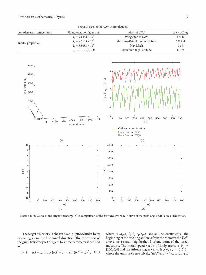Theses analyses are important particularly in the trackingprocess of aircrafts [23 24] So in this paper some discussionshave been made to provide clear relationships between Liegroups SO(3) and SE(3) and their Lie algebras 119904119900(3) and 119904119890(3)Then some features of the error functions on SO(3) are provedbefore a new designed error function on SE(3) is proposedThus a new way of error functions constructing is presentedThe effects of the different error functions are tested in thesimulation with a 6-DOF UAV model

2 Preliminary

21 UAVModel A flight control system is a bit more compli-cated than ordinary control systemsThe analytic expressionsof 6-DOF motion of an aircraft that is the 12 nonlineardifferential equations are formulated as follows

(I) Force equations = V119903 minus 119908119902 minus 119892 sin 120579 + 119865119909119898119888

V = minus119906119903 + 119908119901 + 119892 cos 120579 sin120601 + 119865119910119898119888

= 119906119902 minus V119901 + 119892 cos 120579 cos120601 + 119865119911119898119888

(1)

(II) Kinematic equations = 119901 + (119902 sin120601 + 119903 cos120601) tan 120579 = 119902 cos120601 minus 119903 sin120601 = (119902 sin120601 + 119903 cos120601)cos 120579 (2)

(III) Moment equations = (1198881119903 + 1198882119901) 119902 + 1198883119871 + 1198884119873 = 1198885119901119903 minus 1198886 (1199012 minus 1199032) + 1198887119872119903 = (1198888119901 minus 1198882119903) 119902 + 1198884119871 + 1198889119873 (3)

where 1198881 = ((119868119910 minus 119868119911)119868119911 minus 1198682119909119911)(119868119909119868119911 minus 1198682119909119911) 1198882 = ((119868119909 minus 119868119910 +119868119911)119868119909119911)(119868119909119868119911 minus 1198682119909119911) 1198883 = 119868119911(119868119909119868119911 minus 1198682119909119911) 1198884 = 119868119909119911(119868119909119868119911 minus 1198682119909119911)1198885 = (119868119911 minus 119868119909)119868119910 1198886 = 119868119909119911119868119910 1198887 = 1119868119910 1198888 = (119868119909(119868119909 minus 119868119910) +1198682119909119911)(119868119909119868119911 minus 1198682119909119911) and 1198889 = 119868119909(119868119909119868119911 minus 1198682119909119911)(IV) Navigation equations119892 = 119906 cos 120579 cos120595 + V (sin120601 sin 120579 cos120595 minus cos120601 sin120595)+ 119908 (sin120601 sin120595 + cos120601 sin 120579 cos120595) 119892 = 119906 cos 120579 sin120595 + V (sin120601 sin 120579 sin120595 + cos120601 cos120595)+ 119908 (minus sin120601 cos120595 + cos120601 sin 120579 sin120595) ℎ119892 = 119906 sin 120579 minus V sin120601 cos 120579 minus 119908 cos120601 cos 120579

(4)

or 119892 = 119881 cos 120574 cos120593119892 = 119881 cos 120574 sin120593ℎ119892 = 119881 sin 120574 (5)

where 119898119888 is the mass of the aircraft 119865119894 (119894 = 119909 119910 119911)represents the force of axes of aircraft-body coordinate framerespectively 119871 119872 and 119873 are moments of body frame 119906V and 119908 are speed components of body frame 120579 120595 and 120601represent pitch angle yaw angle and bank angle respectively119901 119902 and 119903 are angular velocity from body frame to inertialframe resolved in body frame 119909119892 119910119892 and ℎ119892 represent theposition of the aircraft in inertial frame 119868119909 119868119910 and 119868119911 arerotary inertias of axes of body frame119881 is true airspeed and 120574120593 are flight-path angles between the firstsecond axis of windcoordinate frame and inertial frame respectively

In practice we may not necessarily choose 119906 V and 119908 asthe state variables of an aircraft model concerning differentrequirements and we usually choose the true air speed 119881 andaerodynamic angles such as angle of attack 120572 and sideslipangle 120573 instead According to the rotation matrix 1198771198822119861from wind frame to body frame along with the relationship119883body = 1198771198822119861119883wind one has the equation

[[[119906V119908]]] = 1198771198822119861

[[[11988100]]] = [[[

119881 cos120572 cos120573119881 sin120573119881 sin120572 cos120573]]] (6)

With (1)sim(4) the 12 differential equations are obtainedhowever it is not adequate to establish a complete nonlinearmodel of a UAV More additional parts are needed Figure 1shows the inner structure of the UAV dynamic model

Here 120575119890 120575119886 and 120575119903 are the angular deviations of theelevator ailerons and rudder 120575119879 is the opening degree ofthrottle and Mach represents Mach number As shown inFigure 1 the actuators are 120575119890 120575119886 120575119903 and 120575119879 rather than forcesand moments Then it is viable to construct a simulationmodel of the given aircraft By (1)sim(4) a nonlinear state-spacesystem can be obtained with state variables defined by X119879 =[119906 V 119908 120601 120579 120595 119901 119902 119903 119909119892 119910119892 ℎ] and control input vector asU119879 = [120575119890 120575120572 120575119903 120575119879]22 Adjoint Representations of Lie Algebras Before the fea-tures of the error functions on SO(3) and SE(3) are discussedthe features of SO(3) and SE(3) themselves should be madeclear In the following part some basic concepts of the screwalgebra and Lie group theory are discussed in detail

According to the screw algebra theory of motions ofthe rigid body the definitions and adjoint representationsof the 3-dimensional special orthogonal group SO(3) the 3-dimensional special Euclidean group SE(3) and the corre-sponding Lie algebras 119904119900(3) and 119904119890(3) are presented as follows

(I) The 3 times 3 matrix adjoint representation of 119904119900(3) is asfollows



of UAV


computing


computing

Enginemodel








120575e 120575a 120575r Fi(i = x y z)

120579 120595 120601 p q r xg yg hg

120574 120593 120572 120573 V Mach

120575T

LMN





ad (s1) = sand1 = [[[0 0 00 0 minus10 1 0 ]]]

ad (s2) = sand2 = [[[0 0 10 0 0minus1 0 0]]]

ad (s3) = sand3 = [[[0 minus1 01 0 00 0 0]]]

(8)





0119879 0 ] (9)


E1 = [[[[[[0 0 0 00 0 minus1 00 1 0 00 0 0 0

]]]]]] E2 = [[[[[[

0 0 1 00 0 0 0minus1 0 0 00 0 0 0]]]]]]

E3 = [[[[[[0 minus1 0 01 0 0 00 0 0 00 0 0 0

]]]]]] E4 = [[[[[[

0 0 0 10 0 0 00 0 0 00 0 0 0]]]]]]

E5 = [[[[[[0 0 0 00 0 0 10 0 0 00 0 0 0

]]]]]] E6 = [[[[[[

0 0 0 00 0 0 00 0 0 10 0 0 0]]]]]]

(10)




] (11)





ad (S4) = [ 0 0sand1 0]

ad (S5) = [ 0 0sand2 0]

ad (S6) = [ 0 0sand3 0]

(12)






defined as

H = 119890120579E = 119890[ 120579A119904 120579s00119879 0 ] = [R d

0119879 1] = [119890120579A119904 Vs00119879 1 ] (14)






SE (3) cong SO (3) prop 119879 (3) (16)



N = [ R 0AR R

] = [ I 0A I

] [R 00 R] = N119905N119903 (17)


detN = det[ R 0AR R

] = detR detR = 1 (18)








P = P sdot G (21)


VandΩ

and] (22)




Φ (RR119889) = 12 tr [I minus R119879119889R] (23)




119889 03times1P119879 minus P119879

119889 1 ] [ R P01times3 1]



119889)P]] (25)


119889R 00 P2 minus P119879119889P

]= 12 tr [I minus R119879

119889R] + 12 (P2 minus P119879119889P)

(26)




Ψ = 12 tr [I minus R119879119889R] + D (27)



119889RΩand] (28)







tr (AB) = tr (BA) (37)

Proof Let



1198871198981 sdot sdot sdot 119887119898119899

) = (119887119894119895) 119894 = 1 2 119898 119895 = 1 2 119899

(38)


119896=1 119886119894119896119887119896119895 119894 119895 = 1 2 119899



tr (AB) = 119899sum119894=1

119888119894119894 = 119899sum119894=1

119898sum119896=1

119886119894119896119887119896119894tr (BA) = 119898sum

119894=1119889119894119894 = 119898sum

119894=1

119899sum119896=1

119887119894119896119886119896119894 = 119899sum119896=1

119898sum119894=1

119886119896119894119887119894119896= 119899sum

119894=1

119898sum119896=1

119886119894119896119887119896119894(39)



tr (A) = tr (A119879) (40)



we have


(42)

Proof finished





Proof finished





119889119877 minus 119877119879119877119889)or Ω (47)





and (49)




(50)

Proof finished





119889119877) 119890Ω (52)


Proof of (52)119889 (119877119879119889119877)119889119905 = 119889 (119877119879

119889)119889119905 119877 + 119877119879119889

119889119877119889119905= minusΩ119889and119877119879

119889119877 + 119877119879119889119877Ωand= 119877119879

119889119877Ωand minus 119877119879119889119877119877119879119877119889Ω119889

and119877119879119889119877= 119877119879


119889119877) 119890Ω(53)

Proof finished


and119889 (119877119879119889)119889119905 = (119889)119879 = (119877119889Ω119889

and)119879 = (Ω119889and)119879 119877119879

119889= minusΩ119889and119877119879

119889 (54)


N = [ R 0AR R

] = N119897N119888 = [ I 0119897A119904 I] [ R 0

rand119890R R] (55)



A119865 ≜ ( 119898sum119894=1

119899sum119895=1

10038161003816100381610038161003816119886119894119895100381610038161003816100381610038162)12 = (tr (A119879A))12 (57)


1003817100381710038171003817119865 = (2 (11990921 + 1199092

2 + 11990923))12 (58)


N = NℎN = [ I 0ℎI I] [ R 0

AR R] = [ R 0

AR R] (59)





or







119889N minus N119879N119889) (63)




UAVmodel

Trajectorygenerator

Trajectoryloops

Attitudeloops

Guidancestrategy



Elevons Drag

Rudders




1198672119868A1198791198670 R119879

1198672119868]] [ R1198612119868 0

A119861R1198612119868 R1198612119868]

minus [R1198791198612119868 R119879

1198612119868A1198791198610 R119879

1198612119868] [ R1198672119868 0

A119867R1198672119868 R1198672119868])

= tr([[R1198791198672119868R1198612119868 + R119879

1198672119868A119879119867A119861R1198612119868 R119879

1198672119868A119879119867R1198612119868

R1198791198672119868A119861R1198612119868 R119879

1198672119868R1198612119868]]minus [R119879

1198612119868R1198672119868 + R1198791198612119868A

119879119861A119867R1198672119868 R119879

1198612119868A119879119861R1198672119868

R1198791198612119868A119867R1198672119868 R119879

1198612119868R1198672119868])

= tr (R1198791198672119868R1198612119868 + R119879

1198672119868A119879119867A119861R1198612119868 minus R119879

1198612119868R1198672119868+ R1198791198612119868A

119879119861A119867R1198672119868 + R119879

1198672119868R1198612119868 minus R1198791198612119868R1198672119868)= tr (2 (R119879

1198672119868R1198612119868 minus R1198791198612119868R1198672119868)+ (R119879

1198672119868A119879119867A119861R1198612119868 minus R119879

1198612119868A119879119861A119867R1198672119868))

(64)

LetM1 = R1198791198672119868R1198612119868 minus R119879

1198612119868R1198672119868 andM2 = R1198791198672119868A

119879119867A119861R1198612119868 minus

R1198791198612119868A




By (30) Ξ2 = minus120596119879119867119861 (2M1 + M2)or (66)








Inertia properties


0

2

0

x-position (m)


2600

2800

3000

3200

3400

z-p

ositi

on (m

)

(a)


minus5

minus4

minus3

minus2

minus1

0

1

x-tr

acki

ng er

ror (

m)

100 200 300 400 500 600 700 800 9000t (s)

(b)

minus10

minus8

minus6

minus4

minus2

0

2

4

6

8

10

100 200 300 400 500 600 700 800 9000t (s)

120579(∘)

(c)

0

500

1000

1500

2000

2500

3000

3500

4000

T(N

)

100 200 300 400 500 600 700 800 9000t (s)

(d)



r (119905) = (1198861119905 + 1198881 1198862 cos (1198871119905) + 1198882 1198863 sin (1198872119905) + 1198883)119879 (67)




(68)





Competing Interests


References


































Volume 2014




Journal of











Journal of


Function Spaces






Algebra











of UAV


computing


computing

Enginemodel








120575e 120575a 120575r Fi(i = x y z)

120579 120595 120601 p q r xg yg hg

120574 120593 120572 120573 V Mach

120575T

LMN





ad (s1) = sand1 = [[[0 0 00 0 minus10 1 0 ]]]

ad (s2) = sand2 = [[[0 0 10 0 0minus1 0 0]]]

ad (s3) = sand3 = [[[0 minus1 01 0 00 0 0]]]

(8)





0119879 0 ] (9)


E1 = [[[[[[0 0 0 00 0 minus1 00 1 0 00 0 0 0

]]]]]] E2 = [[[[[[

0 0 1 00 0 0 0minus1 0 0 00 0 0 0]]]]]]

E3 = [[[[[[0 minus1 0 01 0 0 00 0 0 00 0 0 0

]]]]]] E4 = [[[[[[

0 0 0 10 0 0 00 0 0 00 0 0 0]]]]]]

E5 = [[[[[[0 0 0 00 0 0 10 0 0 00 0 0 0

]]]]]] E6 = [[[[[[

0 0 0 00 0 0 00 0 0 10 0 0 0]]]]]]

(10)




] (11)





ad (S4) = [ 0 0sand1 0]

ad (S5) = [ 0 0sand2 0]

ad (S6) = [ 0 0sand3 0]

(12)






defined as

H = 119890120579E = 119890[ 120579A119904 120579s00119879 0 ] = [R d

0119879 1] = [119890120579A119904 Vs00119879 1 ] (14)






SE (3) cong SO (3) prop 119879 (3) (16)



N = [ R 0AR R

] = [ I 0A I

] [R 00 R] = N119905N119903 (17)


detN = det[ R 0AR R

] = detR detR = 1 (18)








P = P sdot G (21)


VandΩ

and] (22)




Φ (RR119889) = 12 tr [I minus R119879119889R] (23)




119889 03times1P119879 minus P119879

119889 1 ] [ R P01times3 1]



119889)P]] (25)


119889R 00 P2 minus P119879119889P

]= 12 tr [I minus R119879

119889R] + 12 (P2 minus P119879119889P)

(26)




Ψ = 12 tr [I minus R119879119889R] + D (27)



119889RΩand] (28)







tr (AB) = tr (BA) (37)

Proof Let



1198871198981 sdot sdot sdot 119887119898119899

) = (119887119894119895) 119894 = 1 2 119898 119895 = 1 2 119899

(38)


119896=1 119886119894119896119887119896119895 119894 119895 = 1 2 119899



tr (AB) = 119899sum119894=1

119888119894119894 = 119899sum119894=1

119898sum119896=1

119886119894119896119887119896119894tr (BA) = 119898sum

119894=1119889119894119894 = 119898sum

119894=1

119899sum119896=1

119887119894119896119886119896119894 = 119899sum119896=1

119898sum119894=1

119886119896119894119887119894119896= 119899sum

119894=1

119898sum119896=1

119886119894119896119887119896119894(39)



tr (A) = tr (A119879) (40)



we have


(42)

Proof finished





Proof finished





119889119877 minus 119877119879119877119889)or Ω (47)





and (49)




(50)

Proof finished





119889119877) 119890Ω (52)


Proof of (52)119889 (119877119879119889119877)119889119905 = 119889 (119877119879

119889)119889119905 119877 + 119877119879119889

119889119877119889119905= minusΩ119889and119877119879

119889119877 + 119877119879119889119877Ωand= 119877119879

119889119877Ωand minus 119877119879119889119877119877119879119877119889Ω119889

and119877119879119889119877= 119877119879


119889119877) 119890Ω(53)

Proof finished


and119889 (119877119879119889)119889119905 = (119889)119879 = (119877119889Ω119889

and)119879 = (Ω119889and)119879 119877119879

119889= minusΩ119889and119877119879

119889 (54)


N = [ R 0AR R

] = N119897N119888 = [ I 0119897A119904 I] [ R 0

rand119890R R] (55)



A119865 ≜ ( 119898sum119894=1

119899sum119895=1

10038161003816100381610038161003816119886119894119895100381610038161003816100381610038162)12 = (tr (A119879A))12 (57)


1003817100381710038171003817119865 = (2 (11990921 + 1199092

2 + 11990923))12 (58)


N = NℎN = [ I 0ℎI I] [ R 0

AR R] = [ R 0

AR R] (59)





or







119889N minus N119879N119889) (63)




UAVmodel

Trajectorygenerator

Trajectoryloops

Attitudeloops

Guidancestrategy



Elevons Drag

Rudders




1198672119868A1198791198670 R119879

1198672119868]] [ R1198612119868 0

A119861R1198612119868 R1198612119868]

minus [R1198791198612119868 R119879

1198612119868A1198791198610 R119879

1198612119868] [ R1198672119868 0

A119867R1198672119868 R1198672119868])

= tr([[R1198791198672119868R1198612119868 + R119879

1198672119868A119879119867A119861R1198612119868 R119879

1198672119868A119879119867R1198612119868

R1198791198672119868A119861R1198612119868 R119879

1198672119868R1198612119868]]minus [R119879

1198612119868R1198672119868 + R1198791198612119868A

119879119861A119867R1198672119868 R119879

1198612119868A119879119861R1198672119868

R1198791198612119868A119867R1198672119868 R119879

1198612119868R1198672119868])

= tr (R1198791198672119868R1198612119868 + R119879

1198672119868A119879119867A119861R1198612119868 minus R119879

1198612119868R1198672119868+ R1198791198612119868A

119879119861A119867R1198672119868 + R119879

1198672119868R1198612119868 minus R1198791198612119868R1198672119868)= tr (2 (R119879

1198672119868R1198612119868 minus R1198791198612119868R1198672119868)+ (R119879

1198672119868A119879119867A119861R1198612119868 minus R119879

1198612119868A119879119861A119867R1198672119868))

(64)

LetM1 = R1198791198672119868R1198612119868 minus R119879

1198612119868R1198672119868 andM2 = R1198791198672119868A

119879119867A119861R1198612119868 minus

R1198791198612119868A




By (30) Ξ2 = minus120596119879119867119861 (2M1 + M2)or (66)








Inertia properties


0

2

0

x-position (m)


2600

2800

3000

3200

3400

z-p

ositi

on (m

)

(a)


minus5

minus4

minus3

minus2

minus1

0

1

x-tr

acki

ng er

ror (

m)

100 200 300 400 500 600 700 800 9000t (s)

(b)

minus10

minus8

minus6

minus4

minus2

0

2

4

6

8

10

100 200 300 400 500 600 700 800 9000t (s)

120579(∘)

(c)

0

500

1000

1500

2000

2500

3000

3500

4000

T(N

)

100 200 300 400 500 600 700 800 9000t (s)

(d)



r (119905) = (1198861119905 + 1198881 1198862 cos (1198871119905) + 1198882 1198863 sin (1198872119905) + 1198883)119879 (67)




(68)





Competing Interests


References


































Volume 2014




Journal of











Journal of


Function Spaces






Algebra












] (11)





ad (S4) = [ 0 0sand1 0]

ad (S5) = [ 0 0sand2 0]

ad (S6) = [ 0 0sand3 0]

(12)






defined as

H = 119890120579E = 119890[ 120579A119904 120579s00119879 0 ] = [R d

0119879 1] = [119890120579A119904 Vs00119879 1 ] (14)






SE (3) cong SO (3) prop 119879 (3) (16)



N = [ R 0AR R

] = [ I 0A I

] [R 00 R] = N119905N119903 (17)


detN = det[ R 0AR R

] = detR detR = 1 (18)








P = P sdot G (21)


VandΩ

and] (22)




Φ (RR119889) = 12 tr [I minus R119879119889R] (23)




119889 03times1P119879 minus P119879

119889 1 ] [ R P01times3 1]



119889)P]] (25)


119889R 00 P2 minus P119879119889P

]= 12 tr [I minus R119879

119889R] + 12 (P2 minus P119879119889P)

(26)




Ψ = 12 tr [I minus R119879119889R] + D (27)



119889RΩand] (28)







tr (AB) = tr (BA) (37)

Proof Let



1198871198981 sdot sdot sdot 119887119898119899

) = (119887119894119895) 119894 = 1 2 119898 119895 = 1 2 119899

(38)


119896=1 119886119894119896119887119896119895 119894 119895 = 1 2 119899



tr (AB) = 119899sum119894=1

119888119894119894 = 119899sum119894=1

119898sum119896=1

119886119894119896119887119896119894tr (BA) = 119898sum

119894=1119889119894119894 = 119898sum

119894=1

119899sum119896=1

119887119894119896119886119896119894 = 119899sum119896=1

119898sum119894=1

119886119896119894119887119894119896= 119899sum

119894=1

119898sum119896=1

119886119894119896119887119896119894(39)



tr (A) = tr (A119879) (40)



we have


(42)

Proof finished





Proof finished





119889119877 minus 119877119879119877119889)or Ω (47)





and (49)




(50)

Proof finished





119889119877) 119890Ω (52)


Proof of (52)119889 (119877119879119889119877)119889119905 = 119889 (119877119879

119889)119889119905 119877 + 119877119879119889

119889119877119889119905= minusΩ119889and119877119879

119889119877 + 119877119879119889119877Ωand= 119877119879

119889119877Ωand minus 119877119879119889119877119877119879119877119889Ω119889

and119877119879119889119877= 119877119879


119889119877) 119890Ω(53)

Proof finished


and119889 (119877119879119889)119889119905 = (119889)119879 = (119877119889Ω119889

and)119879 = (Ω119889and)119879 119877119879

119889= minusΩ119889and119877119879

119889 (54)


N = [ R 0AR R

] = N119897N119888 = [ I 0119897A119904 I] [ R 0

rand119890R R] (55)



A119865 ≜ ( 119898sum119894=1

119899sum119895=1

10038161003816100381610038161003816119886119894119895100381610038161003816100381610038162)12 = (tr (A119879A))12 (57)


1003817100381710038171003817119865 = (2 (11990921 + 1199092

2 + 11990923))12 (58)


N = NℎN = [ I 0ℎI I] [ R 0

AR R] = [ R 0

AR R] (59)





or







119889N minus N119879N119889) (63)




UAVmodel

Trajectorygenerator

Trajectoryloops

Attitudeloops

Guidancestrategy



Elevons Drag

Rudders




1198672119868A1198791198670 R119879

1198672119868]] [ R1198612119868 0

A119861R1198612119868 R1198612119868]

minus [R1198791198612119868 R119879

1198612119868A1198791198610 R119879

1198612119868] [ R1198672119868 0

A119867R1198672119868 R1198672119868])

= tr([[R1198791198672119868R1198612119868 + R119879

1198672119868A119879119867A119861R1198612119868 R119879

1198672119868A119879119867R1198612119868

R1198791198672119868A119861R1198612119868 R119879

1198672119868R1198612119868]]minus [R119879

1198612119868R1198672119868 + R1198791198612119868A

119879119861A119867R1198672119868 R119879

1198612119868A119879119861R1198672119868

R1198791198612119868A119867R1198672119868 R119879

1198612119868R1198672119868])

= tr (R1198791198672119868R1198612119868 + R119879

1198672119868A119879119867A119861R1198612119868 minus R119879

1198612119868R1198672119868+ R1198791198612119868A

119879119861A119867R1198672119868 + R119879

1198672119868R1198612119868 minus R1198791198612119868R1198672119868)= tr (2 (R119879

1198672119868R1198612119868 minus R1198791198612119868R1198672119868)+ (R119879

1198672119868A119879119867A119861R1198612119868 minus R119879

1198612119868A119879119861A119867R1198672119868))

(64)

LetM1 = R1198791198672119868R1198612119868 minus R119879

1198612119868R1198672119868 andM2 = R1198791198672119868A

119879119867A119861R1198612119868 minus

R1198791198612119868A




By (30) Ξ2 = minus120596119879119867119861 (2M1 + M2)or (66)








Inertia properties


0

2

0

x-position (m)


2600

2800

3000

3200

3400

z-p

ositi

on (m

)

(a)


minus5

minus4

minus3

minus2

minus1

0

1

x-tr

acki

ng er

ror (

m)

100 200 300 400 500 600 700 800 9000t (s)

(b)

minus10

minus8

minus6

minus4

minus2

0

2

4

6

8

10

100 200 300 400 500 600 700 800 9000t (s)

120579(∘)

(c)

0

500

1000

1500

2000

2500

3000

3500

4000

T(N

)

100 200 300 400 500 600 700 800 9000t (s)

(d)



r (119905) = (1198861119905 + 1198881 1198862 cos (1198871119905) + 1198882 1198863 sin (1198872119905) + 1198883)119879 (67)




(68)





Competing Interests


References


































Volume 2014




Journal of











Journal of


Function Spaces






Algebra











Φ (RR119889) = 12 tr [I minus R119879119889R] (23)




119889 03times1P119879 minus P119879

119889 1 ] [ R P01times3 1]



119889)P]] (25)


119889R 00 P2 minus P119879119889P

]= 12 tr [I minus R119879

119889R] + 12 (P2 minus P119879119889P)

(26)




Ψ = 12 tr [I minus R119879119889R] + D (27)



119889RΩand] (28)







tr (AB) = tr (BA) (37)

Proof Let



1198871198981 sdot sdot sdot 119887119898119899

) = (119887119894119895) 119894 = 1 2 119898 119895 = 1 2 119899

(38)


119896=1 119886119894119896119887119896119895 119894 119895 = 1 2 119899



tr (AB) = 119899sum119894=1

119888119894119894 = 119899sum119894=1

119898sum119896=1

119886119894119896119887119896119894tr (BA) = 119898sum

119894=1119889119894119894 = 119898sum

119894=1

119899sum119896=1

119887119894119896119886119896119894 = 119899sum119896=1

119898sum119894=1

119886119896119894119887119894119896= 119899sum

119894=1

119898sum119896=1

119886119894119896119887119896119894(39)



tr (A) = tr (A119879) (40)



we have


(42)

Proof finished





Proof finished





119889119877 minus 119877119879119877119889)or Ω (47)





and (49)




(50)

Proof finished





119889119877) 119890Ω (52)


Proof of (52)119889 (119877119879119889119877)119889119905 = 119889 (119877119879

119889)119889119905 119877 + 119877119879119889

119889119877119889119905= minusΩ119889and119877119879

119889119877 + 119877119879119889119877Ωand= 119877119879

119889119877Ωand minus 119877119879119889119877119877119879119877119889Ω119889

and119877119879119889119877= 119877119879


119889119877) 119890Ω(53)

Proof finished


and119889 (119877119879119889)119889119905 = (119889)119879 = (119877119889Ω119889

and)119879 = (Ω119889and)119879 119877119879

119889= minusΩ119889and119877119879

119889 (54)


N = [ R 0AR R

] = N119897N119888 = [ I 0119897A119904 I] [ R 0

rand119890R R] (55)



A119865 ≜ ( 119898sum119894=1

119899sum119895=1

10038161003816100381610038161003816119886119894119895100381610038161003816100381610038162)12 = (tr (A119879A))12 (57)


1003817100381710038171003817119865 = (2 (11990921 + 1199092

2 + 11990923))12 (58)


N = NℎN = [ I 0ℎI I] [ R 0

AR R] = [ R 0

AR R] (59)





or







119889N minus N119879N119889) (63)




UAVmodel

Trajectorygenerator

Trajectoryloops

Attitudeloops

Guidancestrategy



Elevons Drag

Rudders




1198672119868A1198791198670 R119879

1198672119868]] [ R1198612119868 0

A119861R1198612119868 R1198612119868]

minus [R1198791198612119868 R119879

1198612119868A1198791198610 R119879

1198612119868] [ R1198672119868 0

A119867R1198672119868 R1198672119868])

= tr([[R1198791198672119868R1198612119868 + R119879

1198672119868A119879119867A119861R1198612119868 R119879

1198672119868A119879119867R1198612119868

R1198791198672119868A119861R1198612119868 R119879

1198672119868R1198612119868]]minus [R119879

1198612119868R1198672119868 + R1198791198612119868A

119879119861A119867R1198672119868 R119879

1198612119868A119879119861R1198672119868

R1198791198612119868A119867R1198672119868 R119879

1198612119868R1198672119868])

= tr (R1198791198672119868R1198612119868 + R119879

1198672119868A119879119867A119861R1198612119868 minus R119879

1198612119868R1198672119868+ R1198791198612119868A

119879119861A119867R1198672119868 + R119879

1198672119868R1198612119868 minus R1198791198612119868R1198672119868)= tr (2 (R119879

1198672119868R1198612119868 minus R1198791198612119868R1198672119868)+ (R119879

1198672119868A119879119867A119861R1198612119868 minus R119879

1198612119868A119879119861A119867R1198672119868))

(64)

LetM1 = R1198791198672119868R1198612119868 minus R119879

1198612119868R1198672119868 andM2 = R1198791198672119868A

119879119867A119861R1198612119868 minus

R1198791198612119868A




By (30) Ξ2 = minus120596119879119867119861 (2M1 + M2)or (66)








Inertia properties


0

2

0

x-position (m)


2600

2800

3000

3200

3400

z-p

ositi

on (m

)

(a)


minus5

minus4

minus3

minus2

minus1

0

1

x-tr

acki

ng er

ror (

m)

100 200 300 400 500 600 700 800 9000t (s)

(b)

minus10

minus8

minus6

minus4

minus2

0

2

4

6

8

10

100 200 300 400 500 600 700 800 9000t (s)

120579(∘)

(c)

0

500

1000

1500

2000

2500

3000

3500

4000

T(N

)

100 200 300 400 500 600 700 800 9000t (s)

(d)



r (119905) = (1198861119905 + 1198881 1198862 cos (1198871119905) + 1198882 1198863 sin (1198872119905) + 1198883)119879 (67)




(68)





Competing Interests


References


































Volume 2014




Journal of











Journal of


Function Spaces






Algebra











tr (AB) = 119899sum119894=1

119888119894119894 = 119899sum119894=1

119898sum119896=1

119886119894119896119887119896119894tr (BA) = 119898sum

119894=1119889119894119894 = 119898sum

119894=1

119899sum119896=1

119887119894119896119886119896119894 = 119899sum119896=1

119898sum119894=1

119886119896119894119887119894119896= 119899sum

119894=1

119898sum119896=1

119886119894119896119887119896119894(39)



tr (A) = tr (A119879) (40)



we have


(42)

Proof finished





Proof finished





119889119877 minus 119877119879119877119889)or Ω (47)





and (49)




(50)

Proof finished





119889119877) 119890Ω (52)


Proof of (52)119889 (119877119879119889119877)119889119905 = 119889 (119877119879

119889)119889119905 119877 + 119877119879119889

119889119877119889119905= minusΩ119889and119877119879

119889119877 + 119877119879119889119877Ωand= 119877119879

119889119877Ωand minus 119877119879119889119877119877119879119877119889Ω119889

and119877119879119889119877= 119877119879


119889119877) 119890Ω(53)

Proof finished


and119889 (119877119879119889)119889119905 = (119889)119879 = (119877119889Ω119889

and)119879 = (Ω119889and)119879 119877119879

119889= minusΩ119889and119877119879

119889 (54)


N = [ R 0AR R

] = N119897N119888 = [ I 0119897A119904 I] [ R 0

rand119890R R] (55)



A119865 ≜ ( 119898sum119894=1

119899sum119895=1

10038161003816100381610038161003816119886119894119895100381610038161003816100381610038162)12 = (tr (A119879A))12 (57)


1003817100381710038171003817119865 = (2 (11990921 + 1199092

2 + 11990923))12 (58)


N = NℎN = [ I 0ℎI I] [ R 0

AR R] = [ R 0

AR R] (59)





or







119889N minus N119879N119889) (63)




UAVmodel

Trajectorygenerator

Trajectoryloops

Attitudeloops

Guidancestrategy



Elevons Drag

Rudders




1198672119868A1198791198670 R119879

1198672119868]] [ R1198612119868 0

A119861R1198612119868 R1198612119868]

minus [R1198791198612119868 R119879

1198612119868A1198791198610 R119879

1198612119868] [ R1198672119868 0

A119867R1198672119868 R1198672119868])

= tr([[R1198791198672119868R1198612119868 + R119879

1198672119868A119879119867A119861R1198612119868 R119879

1198672119868A119879119867R1198612119868

R1198791198672119868A119861R1198612119868 R119879

1198672119868R1198612119868]]minus [R119879

1198612119868R1198672119868 + R1198791198612119868A

119879119861A119867R1198672119868 R119879

1198612119868A119879119861R1198672119868

R1198791198612119868A119867R1198672119868 R119879

1198612119868R1198672119868])

= tr (R1198791198672119868R1198612119868 + R119879

1198672119868A119879119867A119861R1198612119868 minus R119879

1198612119868R1198672119868+ R1198791198612119868A

119879119861A119867R1198672119868 + R119879

1198672119868R1198612119868 minus R1198791198612119868R1198672119868)= tr (2 (R119879

1198672119868R1198612119868 minus R1198791198612119868R1198672119868)+ (R119879

1198672119868A119879119867A119861R1198612119868 minus R119879

1198612119868A119879119861A119867R1198672119868))

(64)

LetM1 = R1198791198672119868R1198612119868 minus R119879

1198612119868R1198672119868 andM2 = R1198791198672119868A

119879119867A119861R1198612119868 minus

R1198791198612119868A




By (30) Ξ2 = minus120596119879119867119861 (2M1 + M2)or (66)








Inertia properties


0

2

0

x-position (m)


2600

2800

3000

3200

3400

z-p

ositi

on (m

)

(a)


minus5

minus4

minus3

minus2

minus1

0

1

x-tr

acki

ng er

ror (

m)

100 200 300 400 500 600 700 800 9000t (s)

(b)

minus10

minus8

minus6

minus4

minus2

0

2

4

6

8

10

100 200 300 400 500 600 700 800 9000t (s)

120579(∘)

(c)

0

500

1000

1500

2000

2500

3000

3500

4000

T(N

)

100 200 300 400 500 600 700 800 9000t (s)

(d)



r (119905) = (1198861119905 + 1198881 1198862 cos (1198871119905) + 1198882 1198863 sin (1198872119905) + 1198883)119879 (67)




(68)





Competing Interests


References


































Volume 2014




Journal of











Journal of


Function Spaces






Algebra













119889119877) 119890Ω (52)


Proof of (52)119889 (119877119879119889119877)119889119905 = 119889 (119877119879

119889)119889119905 119877 + 119877119879119889

119889119877119889119905= minusΩ119889and119877119879

119889119877 + 119877119879119889119877Ωand= 119877119879

119889119877Ωand minus 119877119879119889119877119877119879119877119889Ω119889

and119877119879119889119877= 119877119879


119889119877) 119890Ω(53)

Proof finished


and119889 (119877119879119889)119889119905 = (119889)119879 = (119877119889Ω119889

and)119879 = (Ω119889and)119879 119877119879

119889= minusΩ119889and119877119879

119889 (54)


N = [ R 0AR R

] = N119897N119888 = [ I 0119897A119904 I] [ R 0

rand119890R R] (55)



A119865 ≜ ( 119898sum119894=1

119899sum119895=1

10038161003816100381610038161003816119886119894119895100381610038161003816100381610038162)12 = (tr (A119879A))12 (57)


1003817100381710038171003817119865 = (2 (11990921 + 1199092

2 + 11990923))12 (58)


N = NℎN = [ I 0ℎI I] [ R 0

AR R] = [ R 0

AR R] (59)





or







119889N minus N119879N119889) (63)




UAVmodel

Trajectorygenerator

Trajectoryloops

Attitudeloops

Guidancestrategy



Elevons Drag

Rudders




1198672119868A1198791198670 R119879

1198672119868]] [ R1198612119868 0

A119861R1198612119868 R1198612119868]

minus [R1198791198612119868 R119879

1198612119868A1198791198610 R119879

1198612119868] [ R1198672119868 0

A119867R1198672119868 R1198672119868])

= tr([[R1198791198672119868R1198612119868 + R119879

1198672119868A119879119867A119861R1198612119868 R119879

1198672119868A119879119867R1198612119868

R1198791198672119868A119861R1198612119868 R119879

1198672119868R1198612119868]]minus [R119879

1198612119868R1198672119868 + R1198791198612119868A

119879119861A119867R1198672119868 R119879

1198612119868A119879119861R1198672119868

R1198791198612119868A119867R1198672119868 R119879

1198612119868R1198672119868])

= tr (R1198791198672119868R1198612119868 + R119879

1198672119868A119879119867A119861R1198612119868 minus R119879

1198612119868R1198672119868+ R1198791198612119868A

119879119861A119867R1198672119868 + R119879

1198672119868R1198612119868 minus R1198791198612119868R1198672119868)= tr (2 (R119879

1198672119868R1198612119868 minus R1198791198612119868R1198672119868)+ (R119879

1198672119868A119879119867A119861R1198612119868 minus R119879

1198612119868A119879119861A119867R1198672119868))

(64)

LetM1 = R1198791198672119868R1198612119868 minus R119879

1198612119868R1198672119868 andM2 = R1198791198672119868A

119879119867A119861R1198612119868 minus

R1198791198612119868A




By (30) Ξ2 = minus120596119879119867119861 (2M1 + M2)or (66)








Inertia properties


0

2

0

x-position (m)


2600

2800

3000

3200

3400

z-p

ositi

on (m

)

(a)


minus5

minus4

minus3

minus2

minus1

0

1

x-tr

acki

ng er

ror (

m)

100 200 300 400 500 600 700 800 9000t (s)

(b)

minus10

minus8

minus6

minus4

minus2

0

2

4

6

8

10

100 200 300 400 500 600 700 800 9000t (s)

120579(∘)

(c)

0

500

1000

1500

2000

2500

3000

3500

4000

T(N

)

100 200 300 400 500 600 700 800 9000t (s)

(d)



r (119905) = (1198861119905 + 1198881 1198862 cos (1198871119905) + 1198882 1198863 sin (1198872119905) + 1198883)119879 (67)




(68)





Competing Interests


References


































Volume 2014




Journal of











Journal of


Function Spaces






Algebra










UAVmodel

Trajectorygenerator

Trajectoryloops

Attitudeloops

Guidancestrategy



Elevons Drag

Rudders




1198672119868A1198791198670 R119879

1198672119868]] [ R1198612119868 0

A119861R1198612119868 R1198612119868]

minus [R1198791198612119868 R119879

1198612119868A1198791198610 R119879

1198612119868] [ R1198672119868 0

A119867R1198672119868 R1198672119868])

= tr([[R1198791198672119868R1198612119868 + R119879

1198672119868A119879119867A119861R1198612119868 R119879

1198672119868A119879119867R1198612119868

R1198791198672119868A119861R1198612119868 R119879

1198672119868R1198612119868]]minus [R119879

1198612119868R1198672119868 + R1198791198612119868A

119879119861A119867R1198672119868 R119879

1198612119868A119879119861R1198672119868

R1198791198612119868A119867R1198672119868 R119879

1198612119868R1198672119868])

= tr (R1198791198672119868R1198612119868 + R119879

1198672119868A119879119867A119861R1198612119868 minus R119879

1198612119868R1198672119868+ R1198791198612119868A

119879119861A119867R1198672119868 + R119879

1198672119868R1198612119868 minus R1198791198612119868R1198672119868)= tr (2 (R119879

1198672119868R1198612119868 minus R1198791198612119868R1198672119868)+ (R119879

1198672119868A119879119867A119861R1198612119868 minus R119879

1198612119868A119879119861A119867R1198672119868))

(64)

LetM1 = R1198791198672119868R1198612119868 minus R119879

1198612119868R1198672119868 andM2 = R1198791198672119868A

119879119867A119861R1198612119868 minus

R1198791198612119868A




By (30) Ξ2 = minus120596119879119867119861 (2M1 + M2)or (66)








Inertia properties


0

2

0

x-position (m)


2600

2800

3000

3200

3400

z-p

ositi

on (m

)

(a)


minus5

minus4

minus3

minus2

minus1

0

1

x-tr

acki

ng er

ror (

m)

100 200 300 400 500 600 700 800 9000t (s)

(b)

minus10

minus8

minus6

minus4

minus2

0

2

4

6

8

10

100 200 300 400 500 600 700 800 9000t (s)

120579(∘)

(c)

0

500

1000

1500

2000

2500

3000

3500

4000

T(N

)

100 200 300 400 500 600 700 800 9000t (s)

(d)



r (119905) = (1198861119905 + 1198881 1198862 cos (1198871119905) + 1198882 1198863 sin (1198872119905) + 1198883)119879 (67)




(68)





Competing Interests


References


































Volume 2014




Journal of











Journal of


Function Spaces






Algebra












Inertia properties


0

2

0

x-position (m)


2600

2800

3000

3200

3400

z-p

ositi

on (m

)

(a)


minus5

minus4

minus3

minus2

minus1

0

1

x-tr

acki

ng er

ror (

m)

100 200 300 400 500 600 700 800 9000t (s)

(b)

minus10

minus8

minus6

minus4

minus2

0

2

4

6

8

10

100 200 300 400 500 600 700 800 9000t (s)

120579(∘)

(c)

0

500

1000

1500

2000

2500

3000

3500

4000

T(N

)

100 200 300 400 500 600 700 800 9000t (s)

(d)



r (119905) = (1198861119905 + 1198881 1198862 cos (1198871119905) + 1198882 1198863 sin (1198872119905) + 1198883)119879 (67)




(68)





Competing Interests


References


































Volume 2014




Journal of











Journal of


Function Spaces






Algebra











(68)





Competing Interests


References


































Volume 2014




Journal of











Journal of


Function Spaces






Algebra




























Volume 2014




Journal of











Journal of


Function Spaces






Algebra
















Volume 2014




Journal of











Journal of


Function Spaces






Algebra









Documents

Some Discussions about the Error Functions on SO(3) and SE ...downloads.hindawi.com/journals/amp/2017/1016530.pdf · loops with controllers of the forces and moments ... and moments